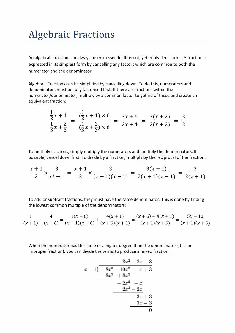
Algebraic Fractions An algebraic fraction can always be expressed in different, yet equivalent forms. A fraction is expressed in its simplest form by cancelling any factors which are common to both the numerator and the denominator. Algebraic Fractions can be simplified by cancelling down. To do this, numerators and denominators must be fully factorised first. If there are fractions within the numerator/denominator, multiply by a common factor to get rid of these and create an equivalent fraction:

12 𝑥 + 113 𝑥 + 2

3 =

(12𝑥 + 1) × 6

(13𝑥 + 2

3) × 6 =

3𝑥 + 62𝑥 + 4 =

3(𝑥 + 2)2(𝑥 + 2) =

32

To multiply fractions, simply multiply the numerators and multiply the denominators. If possible, cancel down first. To divide by a fraction, multiply by the reciprocal of the fraction:

𝑥 + 12 ×

3𝑥2 − 1 =

𝑥 + 12 ×

3(𝑥 + 1)(𝑥 − 1) =

3(𝑥 + 1)2(𝑥 + 1)(𝑥 − 1) =

32(𝑥 + 1)

To add or subtract fractions, they must have the same denominator. This is done by finding the lowest common multiple of the denominators:

1(𝑥 + 1)

+4

(𝑥 + 6)=

1(𝑥 + 6)(𝑥 + 1)(𝑥 + 6)

+4(𝑥 + 1)

(𝑥 + 6)(𝑥 + 1)=

(𝑥 + 6) + 4(𝑥 + 1)(𝑥 + 1)(𝑥 + 6)

=5𝑥 + 10

(𝑥 + 1)(𝑥 + 6)

When the numerator has the same or a higher degree than the denominator (it is an improper fraction), you can divide the terms to produce a mixed fraction:

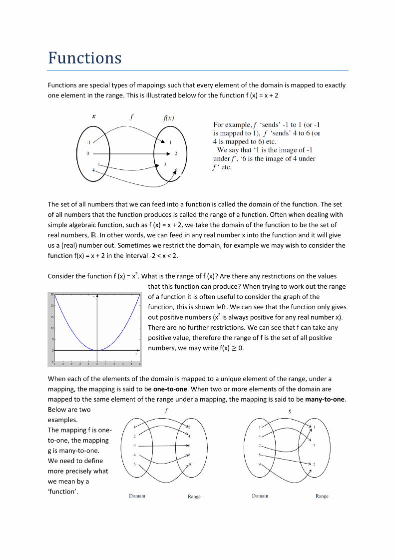
Functions Functions are special types of mappings such that every element of the domain is mapped to exactly one element in the range. This is illustrated below for the function f (x) = x + 2

The set of all numbers that we can feed into a function is called the domain of the function. The set of all numbers that the function produces is called the range of a function. Often when dealing with simple algebraic function, such as f (x) = x + 2, we take the domain of the function to be the set of real numbers, ℝ. In other words, we can feed in any real number x into the function and it will give us a (real) number out. Sometimes we restrict the domain, for example we may wish to consider the function f(x) = x + 2 in the interval -2 < x < 2. Consider the function f (x) = x2. What is the range of f (x)? Are there any restrictions on the values

that this function can produce? When trying to work out the range of a function it is often useful to consider the graph of the function, this is shown left. We can see that the function only gives out positive numbers (x2 is always positive for any real number x). There are no further restrictions. We can see that f can take any positive value, therefore the range of f is the set of all positive numbers, we may write f(x) ≥ 0.

When each of the elements of the domain is mapped to a unique element of the range, under a mapping, the mapping is said to be one-to-one. When two or more elements of the domain are mapped to the same element of the range under a mapping, the mapping is said to be many-to-one. Below are two examples. The mapping f is one-to-one, the mapping g is many-to-one. We need to define more precisely what we mean by a ‘function’.

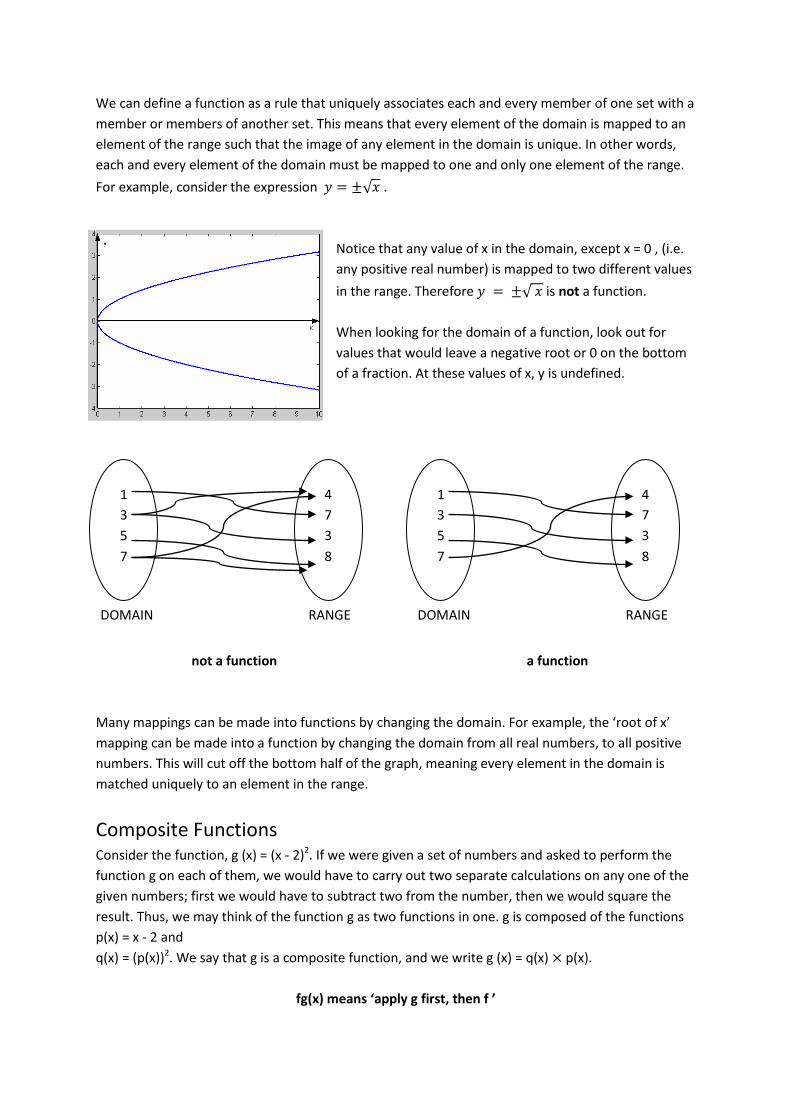
We can define a function as a rule that uniquely associates each and every member of one set with a member or members of another set. This means that every element of the domain is mapped to an element of the range such that the image of any element in the domain is unique. In other words, each and every element of the domain must be mapped to one and only one element of the range. For example, consider the expression 𝑦 = ±√𝑥 .

Notice that any value of x in the domain, except x = 0 , (i.e. any positive real number) is mapped to two different values in the range. Therefore 𝑦 = ±√ 𝑥 is not a function. When looking for the domain of a function, look out for values that would leave a negative root or 0 on the bottom of a fraction. At these values of x, y is undefined.

not a function a function Many mappings can be made into functions by changing the domain. For example, the ‘root of x’ mapping can be made into a function by changing the domain from all real numbers, to all positive numbers. This will cut off the bottom half of the graph, meaning every element in the domain is matched uniquely to an element in the range.

Composite Functions Consider the function, g (x) = (x - 2)2. If we were given a set of numbers and asked to perform the function g on each of them, we would have to carry out two separate calculations on any one of the given numbers; first we would have to subtract two from the number, then we would square the result. Thus, we may think of the function g as two functions in one. g is composed of the functions p(x) = x - 2 and q(x) = (p(x))2. We say that g is a composite function, and we write g (x) = q(x) × p(x).

fg(x) means ‘apply g first, then f ’

DOMAIN RANGE

1 3 5 7

4 7 3 8

DOMAIN RANGE

1 3 5 7

4 7 3 8

Inverse Functions Consider the simple, linear function f (x) = 3x - 27. If we feed x = 2 into this function, we get out f

(2) = -21. Suppose that we are told that the function has produced the number 9, but we do not

know what input produced this number. We can easily work out the input number:

𝑓(𝑛) = 3𝑛 − 27 = 9 → 𝑛 =9 + 27

3= 12

If we know the output of a given function and we require the input of the function, we can find it by using the inverse function. The inverse of a function f(x) is written f-1(x), and performs the opposite operation(s) to the function. There are two methods to find the inverse of a function:

• Work Backwards − We can think of a ‘function machine’ which takes an input, performs the

function on it and produces an output. The inverse function machine takes the output from the original function and gives us the original input number.

• Change the Subject − Let y = f(x), and then rearrange the formulae to find x. You then swap x and y

(y being f(x)). For example, g(x) = 4x – 3, so let y = 4x – 3.

Rearranged to find x gives 𝑓(𝑥) = 𝑥+34

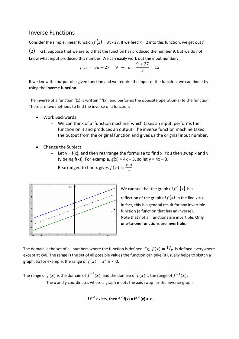
We can see that the graph of f -1 (x) is a

reflection of the graph of f (x) in the line y = x . In fact, this is a general result for any invertible function (a function that has an inverse). Note that not all functions are invertible. Only one-to-one functions are invertible.

The domain is the set of all numbers where the function is defined. Eg, 𝑓(𝑥) = 1 𝑥� is defined everywhere except at x=0. The range is the set of all possible values the function can take (it usually helps to sketch a graph. So for example, the range of 𝑓(𝑥) = 𝑥2 is x>0.

The range of 𝑓(𝑥) is the domain of 𝑓−1(𝑥), and the domain of 𝑓(𝑥) is the range of 𝑓−1(𝑥). The x and y coordinates where a graph meets the axis swap for the inverse graph.

If f −1 exists, then f −1f(x) = ff −1(x) = x.

The Modulus Function

The modulus sign indicates that we take the absolute value of the expression inside the modulus sign, i.e. all values are positive. e.g. |2 − 3| = 1, | 0 − 5| = 5, |−2| = 2, |1 + 7| = 8. We can define:

|𝑥| = �−𝑥, 𝑥 < 0𝑥, 𝑥 ≥ 0

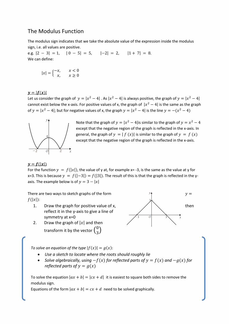
𝒚 = |𝒇(𝒙)| Let us consider the graph of 𝑦 = |𝑥2 − 4| . As |𝑥2 − 4| is always positive, the graph of 𝑦 = |𝑥2 − 4| cannot exist below the x-axis. For positive values of x, the graph of |𝑥2 − 4| is the same as the graph of 𝑦 = |𝑥2 − 4|; but for negative values of x, the graph 𝑦 = |𝑥2 − 4| is the line 𝑦 = −(𝑥2 − 4)

Note that the graph of 𝑦 = |𝑥2 − 4|is similar to the graph of 𝑦 = 𝑥2 − 4 except that the negative region of the graph is reflected in the x-axis. In general, the graph of 𝑦 = | 𝑓 (𝑥)| is similar to the graph of 𝑦 = 𝑓 (𝑥) except that the negative region of the graph is reflected in the x-axis.

𝒚 = 𝒇(|𝒙|) For the function 𝑦 = 𝑓(|𝑥|), the value of y at, for example x= -3, is the same as the value at y for x=3. This is because 𝑦 = 𝑓(|−3|) = 𝑓(|3|). The result of this is that the graph is reflected in the y-axis. The example below is of 𝑦 = 3 − |𝑥| There are two ways to sketch graphs of the form 𝑦 =𝑓(|𝑥|):

1. Draw the graph for positive value of x, then reflect it in the y-axis to give a line of symmetry at x=0

2. Draw the graph of |𝑥| and then

transform it by the vector �03�

To solve an equation of the type |𝑓(𝑥)| = 𝑔(𝑥): • Use a sketch to locate where the roots should roughly lie • Solve algebraically, using −𝑓(𝑥) for reflected parts of 𝑦 = 𝑓(𝑥) and −𝑔(𝑥) for

reflected parts of 𝑦 = 𝑔(𝑥) To solve the equation |𝑎𝑥 + 𝑏| = |𝑐𝑥 + 𝑑| it is easiest to square both sides to remove the modulus sign. Equations of the form |𝑎𝑥 + 𝑏| = 𝑐𝑥 + 𝑑 need to be solved graphically.

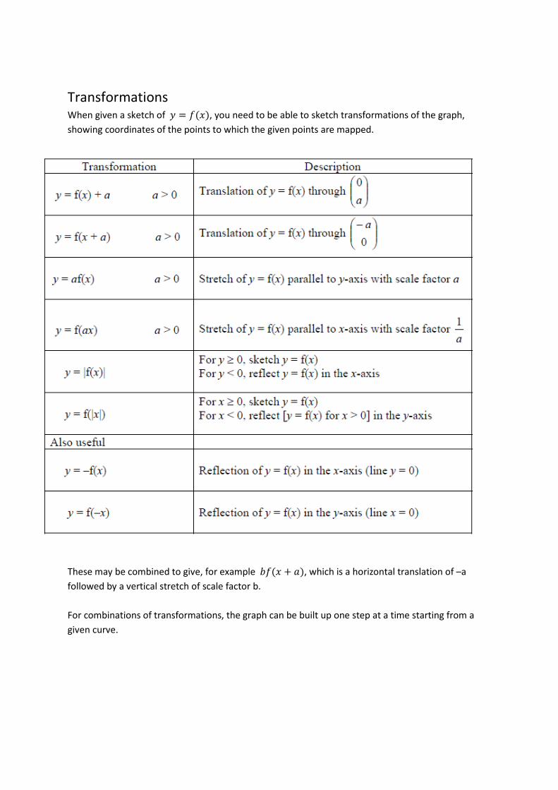
Transformations When given a sketch of 𝑦 = 𝑓(𝑥), you need to be able to sketch transformations of the graph, showing coordinates of the points to which the given points are mapped.

These may be combined to give, for example 𝑏𝑓(𝑥 + 𝑎), which is a horizontal translation of –a followed by a vertical stretch of scale factor b. For combinations of transformations, the graph can be built up one step at a time starting from a given curve.

Numerical Methods In real life situations, we are often faced with equations which have no analytic solution. That is to say we cannot find an exact solution to the equation. For example, we can solve the equation 𝑥2 + 𝑥 − 2 = 0 by factorising (𝑥 + 2)(𝑥 − 1) = 0 𝑥 = −2 or 𝑥 = 1. The above equation can be solved analytically to find the exact solutions. What about the equation 𝑐𝑜𝑠 (𝑥) − 𝑥 = 0 . This equation cannot be solved analytically unlike the previous example. We cannot find the exact solution of this equation using algebraic, or any other techniques. We cannot solve this equation exactly, however we can find the approximate solution or solutions to the equation 𝑐𝑜𝑠 (𝑥) − 𝑥 = 0 . In fact, we can find the solution or solutions to an arbitrary degree of accuracy, however the more accurate we require our solution(s), the longer the process. There are 3 numerical methods that can be used to find approximations to the root(s) of a function which may not be possible to find analytically:

1. Graphically 2. Looking for a change of sign 3. Iteration

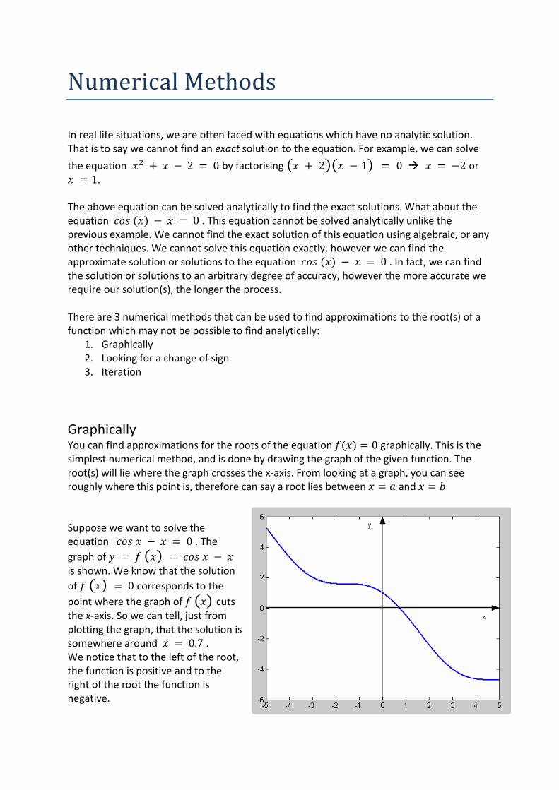
Graphically You can find approximations for the roots of the equation 𝑓(𝑥) = 0 graphically. This is the simplest numerical method, and is done by drawing the graph of the given function. The root(s) will lie where the graph crosses the x-axis. From looking at a graph, you can see roughly where this point is, therefore can say a root lies between 𝑥 = 𝑎 and 𝑥 = 𝑏 Suppose we want to solve the equation 𝑐𝑜𝑠 𝑥 − 𝑥 = 0 . The graph of 𝑦 = 𝑓 (𝑥) = 𝑐𝑜𝑠 𝑥 − 𝑥 is shown. We know that the solution of 𝑓 (𝑥) = 0 corresponds to the point where the graph of 𝑓 (𝑥) cuts the x-axis. So we can tell, just from plotting the graph, that the solution is somewhere around 𝑥 = 0.7 . We notice that to the left of the root, the function is positive and to the right of the root the function is negative.

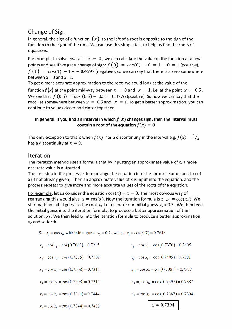
Change of Sign In general, the sign of a function, (𝑥), to the left of a root is opposite to the sign of the function to the right of the root. We can use this simple fact to help us find the roots of equations.

For example to solve 𝑐𝑜𝑠 𝑥 − 𝑥 = 0 , we can calculate the value of the function at a few points and see if we get a change of sign: 𝑓 (0) = 𝑐𝑜𝑠(0) − 0 = 1 − 0 = 1 (positive), 𝑓 (1) = 𝑐𝑜𝑠(1) − 1 » − 0.4597 (negative), so we can say that there is a zero somewhere between x = 0 and x =1. To get a more accurate approximation to the root, we could look at the value of the function f (x) at the point mid-way between 𝑥 = 0 and 𝑥 = 1, i.e. at the point 𝑥 = 0.5 . We see that 𝑓 (0.5) = 𝑐𝑜𝑠 (0.5) − 0.5 = 0.3776 (positive). So now we can say that the root lies somewhere between 𝑥 = 0.5 and 𝑥 = 1. To get a better approximation, you can continue to values closer and closer together.

In general, if you find an interval in which 𝒇(𝒙) changes sign, then the interval must

contain a root of the equation 𝒇(𝒙) = 𝟎

The only exception to this is when 𝑓(𝑥) has a discontinuity in the interval e.g. 𝑓(𝑥) = 1 𝑥� has a discontinuity at 𝑥 = 0. Iteration The iteration method uses a formula that by inputting an approximate value of x, a more accurate value is outputted. The first step in the process is to rearrange the equation into the form x = some function of x (if not already given). Then an approximate value of x is input into the equation, and the process repeats to give more and more accurate values of the roots of the equation.

For example, let us consider the equation cos(𝑥) − 𝑥 = 0. The most obvious way of rearranging this would give 𝑥 = cos (𝑥). Now the iteration formula is 𝑥𝑛+1 = cos (𝑥𝑛). We start with an initial guess to the root x0. Let us make our initial guess x0 = 0.7 . We then feed the initial guess into the iteration formula, to produce a better approximation of the solution, x1 . We then feed x1 into the iteration formula to produce a better approximation,

x2 and so forth.

𝑥 ≈ 0.7394

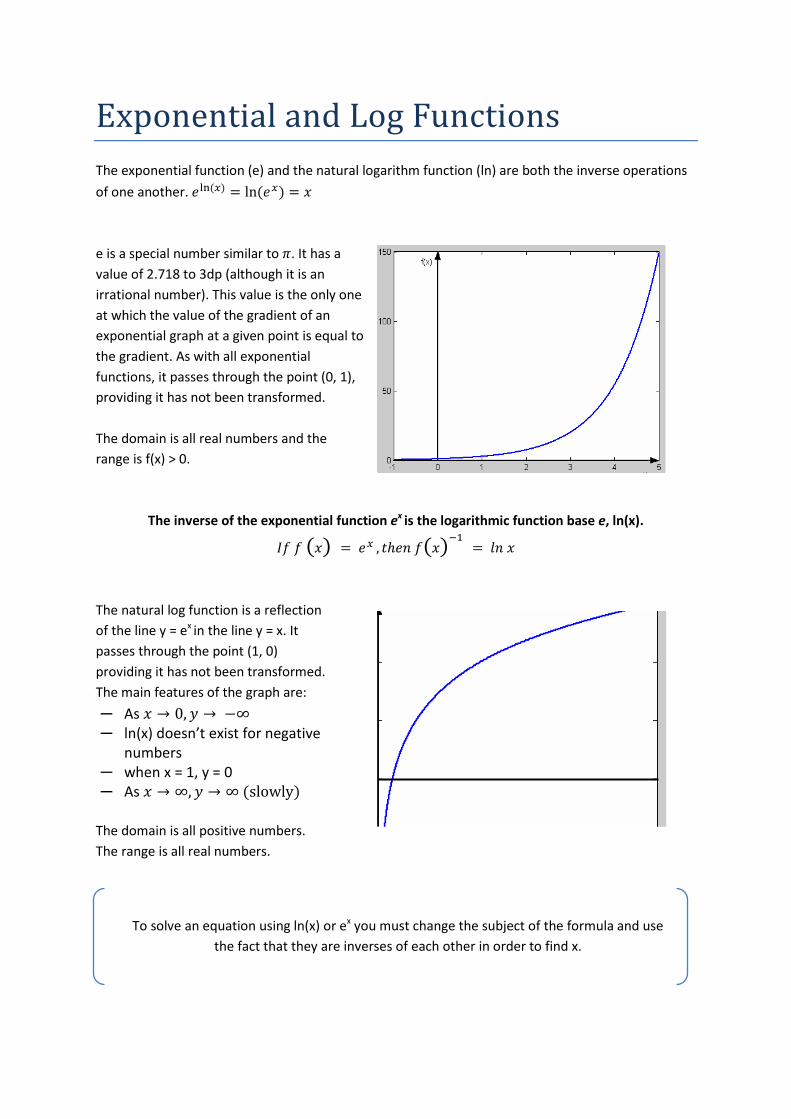
Exponential and Log Functions The exponential function (e) and the natural logarithm function (ln) are both the inverse operations of one another. 𝑒ln (𝑥) = ln (𝑒𝑥) = 𝑥 e is a special number similar to 𝜋. It has a value of 2.718 to 3dp (although it is an irrational number). This value is the only one at which the value of the gradient of an exponential graph at a given point is equal to the gradient. As with all exponential functions, it passes through the point (0, 1), providing it has not been transformed. The domain is all real numbers and the range is f(x) > 0.

The inverse of the exponential function ex is the logarithmic function base e, ln(x).

𝐼𝑓 𝑓 (𝑥) = 𝑒𝑥 , 𝑡ℎ𝑒𝑛 𝑓(𝑥)−1 = 𝑙𝑛 𝑥 The natural log function is a reflection of the line y = ex in the line y = x. It passes through the point (1, 0) providing it has not been transformed. The main features of the graph are: ─ As 𝑥 → 0,𝑦 → −∞ ─ ln(x) doesn’t exist for negative

numbers ─ when x = 1, y = 0 ─ As 𝑥 → ∞,𝑦 → ∞ (slowly)

The domain is all positive numbers. The range is all real numbers.

To solve an equation using ln(x) or ex you must change the subject of the formula and use the fact that they are inverses of each other in order to find x.

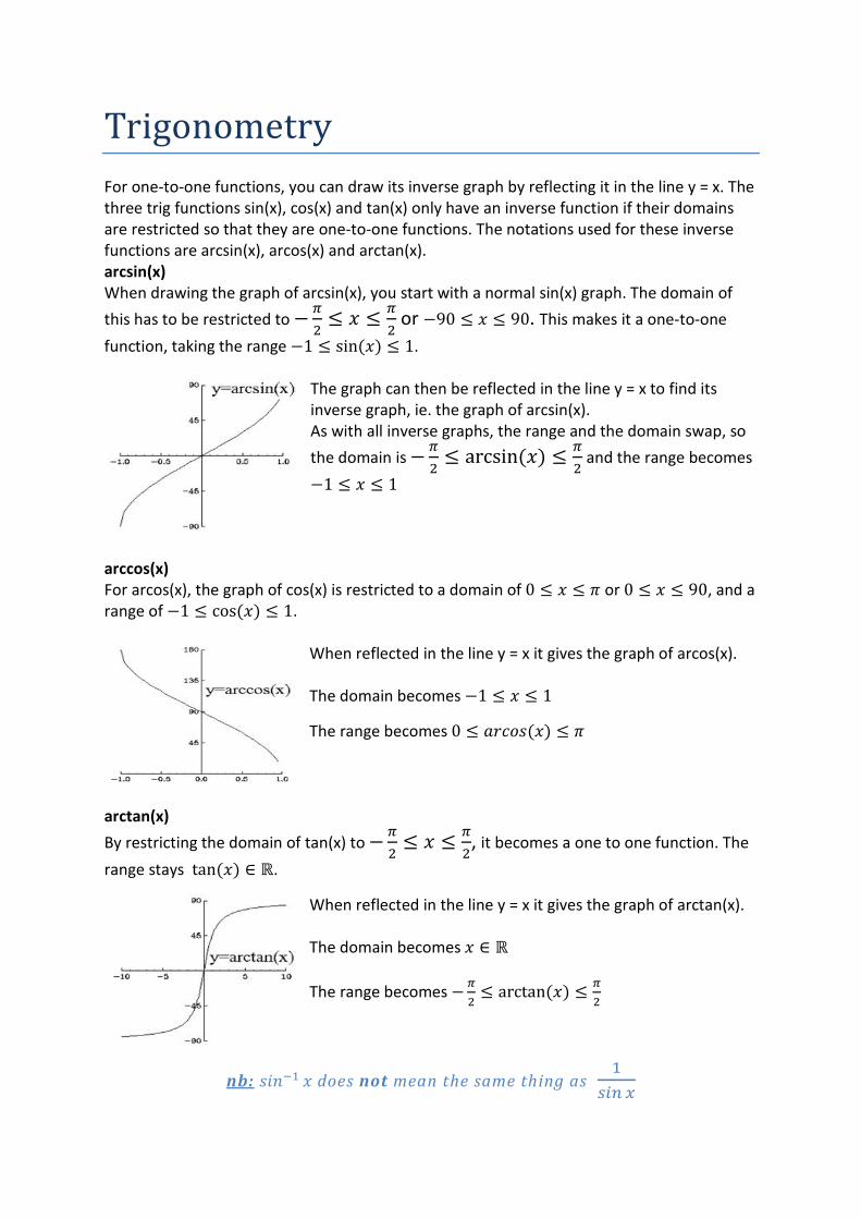
Trigonometry For one-to-one functions, you can draw its inverse graph by reflecting it in the line y = x. The three trig functions sin(x), cos(x) and tan(x) only have an inverse function if their domains are restricted so that they are one-to-one functions. The notations used for these inverse functions are arcsin(x), arcos(x) and arctan(x). arcsin(x) When drawing the graph of arcsin(x), you start with a normal sin(x) graph. The domain of this has to be restricted to −𝜋

2≤ 𝑥 ≤ 𝜋

2 or −90 ≤ 𝑥 ≤ 90. This makes it a one-to-one

function, taking the range −1 ≤ sin (𝑥) ≤ 1.

The graph can then be reflected in the line y = x to find its inverse graph, ie. the graph of arcsin(x). As with all inverse graphs, the range and the domain swap, so the domain is −𝜋

2≤ arcsin (𝑥) ≤ 𝜋

2 and the range becomes

−1 ≤ 𝑥 ≤ 1

arccos(x) For arcos(x), the graph of cos(x) is restricted to a domain of 0 ≤ 𝑥 ≤ 𝜋 or 0 ≤ 𝑥 ≤ 90, and a range of −1 ≤ cos (𝑥) ≤ 1.

When reflected in the line y = x it gives the graph of arcos(x). The domain becomes −1 ≤ 𝑥 ≤ 1

The range becomes 0 ≤ 𝑎𝑟𝑐𝑜𝑠(𝑥) ≤ 𝜋

arctan(x) By restricting the domain of tan(x) to −𝜋

2≤ 𝑥 ≤ 𝜋

2, it becomes a one to one function. The

range stays tan (𝑥) ∈ ℝ.

When reflected in the line y = x it gives the graph of arctan(x). The domain becomes 𝑥 ∈ ℝ The range becomes −𝜋

2≤ arctan (𝑥) ≤ 𝜋

2

nb: 𝑠𝑖𝑛−1 𝑥 does not mean the same thing as 1

𝑠𝑖𝑛 𝑥

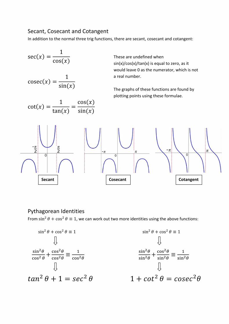
Secant, Cosecant and Cotangent In addition to the normal three trig functions, there are secant, cosecant and cotangent:

sec(𝑥) =1

cos(𝑥)

cosec(𝑥) =1

sin (𝑥)

cot(𝑥) =1

tan (𝑥)=

cos(𝑥)sin (𝑥)

Pythagorean Identities From sin2 𝜃 + cos2 𝜃 ≡ 1, we can work out two more identities using the above functions: sin2 𝜃 + cos2 𝜃 ≡ 1 sin2 𝜃 + cos2 𝜃 ≡ 1

sin2𝜃

cos2 𝜃+ cos2𝜃

cos2𝜃≡ 1

cos2𝜃

sin2𝜃sin2𝜃

+ cos2𝜃sin2𝜃

≡ 1sin2𝜃

𝑡𝑎𝑛2 𝜃 + 1 = 𝑠𝑒𝑐2 𝜃 1 + 𝑐𝑜𝑡2 𝜃 = 𝑐𝑜𝑠𝑒𝑐2𝜃

These are undefined when sin(x)/cos(x)/tan(x) is equal to zero, as it would leave 0 as the numerator, which is not a real number. The graphs of these functions are found by plotting points using these formulae.

Secant Cosecant Cotangent

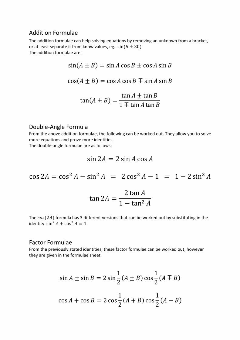
Addition Formulae The addition formulae can help solving equations by removing an unknown from a bracket, or at least separate it from know values, eg. sin (𝜃 + 30) The addition formulae are:

sin(𝐴 ± 𝐵) = sin𝐴 cos𝐵 ± cos𝐴 sin𝐵

cos(𝐴 ± 𝐵) = cos𝐴 cos𝐵 ∓ sin𝐴 sin𝐵

tan(𝐴 ± 𝐵) =tan𝐴 ± tan𝐵

1 ∓ tan𝐴 tan𝐵

Double-Angle Formula From the above addition formulae, the following can be worked out. They allow you to solve more equations and prove more identities. The double-angle formulae are as follows:

sin 2𝐴 = 2 sin𝐴 cos𝐴 cos 2𝐴 = cos2 𝐴 − sin2 𝐴 = 2 cos2 𝐴 − 1 = 1 − 2 sin2 𝐴

tan 2𝐴 =2 tan𝐴

1 − tan2 𝐴

The 𝑐𝑜𝑠(2𝐴) formula has 3 different versions that can be worked out by substituting in the identity sin2 𝐴 + cos2 𝐴 = 1. Factor Formulae From the previously stated identities, these factor formulae can be worked out, however they are given in the formulae sheet.

sin𝐴 ± sin𝐵 = 2 sin12

(𝐴 ± 𝐵) cos12

(𝐴 ∓ 𝐵)

cos𝐴 + cos𝐵 = 2 cos12

(𝐴 + 𝐵) cos12

(𝐴 − 𝐵)

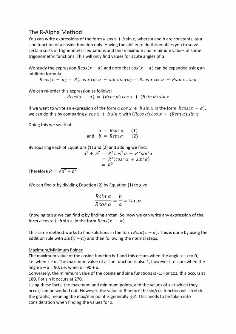
The R-Alpha Method You can write expressions of the form 𝑎 cos 𝑥 + 𝑏 sin 𝑥, where a and b are constants, as a sine function or a cosine function only. Having the ability to do this enables you to solve certain sorts of trigonometric equations and find maximum and minimum values of some trigonometric functions. This will only find values for acute angles of α. We study the expression 𝑅𝑐𝑜𝑠(𝑥 − 𝛼) and note that 𝑐𝑜𝑠(𝑥 − 𝛼) can be expanded using an addition formula.

𝑅𝑐𝑜𝑠(𝑥 − 𝛼) = 𝑅(𝑐𝑜𝑠 𝑥 cos𝛼 + 𝑠𝑖𝑛 𝑥 sin𝛼) = 𝑅𝑐𝑜𝑠 𝑥 cos𝛼 + 𝑅𝑠𝑖𝑛 𝑥 𝑠𝑖𝑛 𝛼 We can re-order this expression as follows:

𝑅𝑐𝑜𝑠(𝑥 − 𝛼) = (𝑅𝑐𝑜𝑠 𝛼) 𝑐𝑜𝑠 𝑥 + (𝑅𝑠𝑖𝑛 𝛼) 𝑠𝑖𝑛 𝑥 If we want to write an expression of the form 𝑎 𝑐𝑜𝑠 𝑥 + 𝑏 𝑠𝑖𝑛 𝑥 in the form 𝑅𝑐𝑜𝑠(𝑥 − 𝛼), we can do this by comparing 𝑎 𝑐𝑜𝑠 𝑥 + 𝑏 𝑠𝑖𝑛 𝑥 with (𝑅𝑐𝑜𝑠 𝛼) 𝑐𝑜𝑠 𝑥 + (𝑅𝑠𝑖𝑛 𝛼) 𝑠𝑖𝑛 𝑥 Doing this we see that

𝑎 = 𝑅𝑐𝑜𝑠 𝛼 (1) and 𝑏 = 𝑅𝑠𝑖𝑛 𝛼 (2)

By squaring each of Equations (1) and (2) and adding we find:

𝑎2 + 𝑏2 = 𝑅2 𝑐𝑜𝑠2 𝛼 + 𝑅 2𝑠𝑖𝑛2𝛼

= 𝑅2(𝑐𝑜𝑠2 𝛼 + 𝑠𝑖𝑛2𝛼) = 𝑅2 Therefore 𝑅 = √𝑎2 + 𝑏2

We can find 𝛼 by dividing Equation (2) by Equation (1) to give

𝑅𝑠𝑖𝑛 𝛼𝑅𝑐𝑜𝑠 𝛼 =

𝑏𝑎 = tan𝛼

Knowing tan𝛼 we can find α by finding arctan. So, now we can write any expression of the form 𝑎 cos 𝑥 + 𝑏 sin 𝑥 in the form 𝑅𝑐𝑜𝑠(𝑥 − 𝛼). This same method works to find solutions in the form 𝑅𝑠𝑖𝑛(𝑥 − 𝛼). This is done by using the addition rule with 𝑠𝑖𝑛(𝑥 − 𝛼) and then following the normal steps. Maximum/Minimum Points: The maximum value of the cosine function is 1 and this occurs when the angle x − α = 0, i.e. when x = α. The maximum value of a sine function is also 1, however it occurs when the angle x – α = 90, i.e. when x = 90 + α. Conversely, the minimum value of the cosine and sine functions is -1. For cos, this occurs at 180. For sin it occurs at 270. Using these facts, the maximum and minimum points, and the values of x at which they occur, can be worked out. However, the value of R before the sin/cos function will stretch the graphs, meaning the max/min point is generally ±𝑅. This needs to be taken into consideration when finding the values for x.

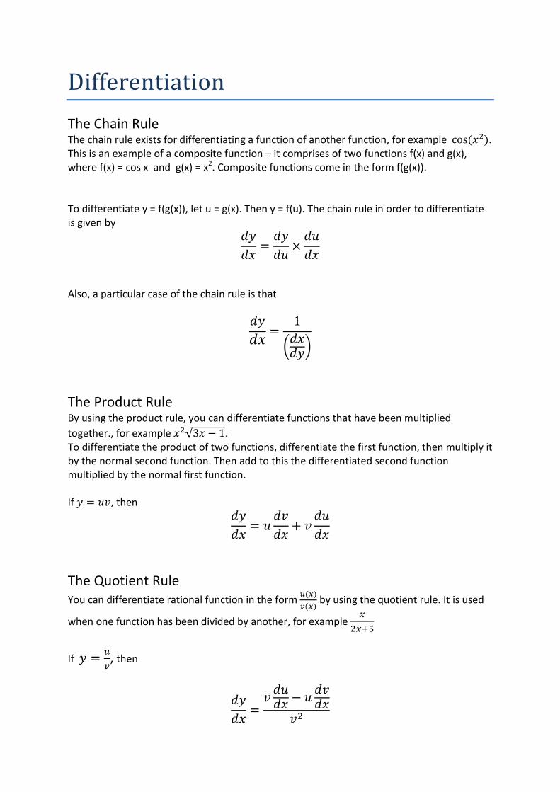
Differentiation The Chain Rule The chain rule exists for differentiating a function of another function, for example cos(𝑥2). This is an example of a composite function – it comprises of two functions f(x) and g(x), where f(x) = cos x and g(x) = x2. Composite functions come in the form f(g(x)). To differentiate y = f(g(x)), let u = g(x). Then y = f(u). The chain rule in order to differentiate is given by

𝑑𝑦𝑑𝑥 =

𝑑𝑦𝑑𝑢 ×

𝑑𝑢𝑑𝑥

Also, a particular case of the chain rule is that

𝑑𝑦𝑑𝑥 =

1

�𝑑𝑥𝑑𝑦�

The Product Rule By using the product rule, you can differentiate functions that have been multiplied together., for example 𝑥2√3𝑥 − 1. To differentiate the product of two functions, differentiate the first function, then multiply it by the normal second function. Then add to this the differentiated second function multiplied by the normal first function. If 𝑦 = 𝑢𝑣, then

𝑑𝑦𝑑𝑥 = 𝑢

𝑑𝑣𝑑𝑥 + 𝑣

𝑑𝑢𝑑𝑥

The Quotient Rule You can differentiate rational function in the form 𝑢(𝑥)

𝑣(𝑥) by using the quotient rule. It is used

when one function has been divided by another, for example 𝑥

2𝑥+5

If 𝑦 = 𝑢

𝑣, then

𝑑𝑦𝑑𝑥 =

𝑣 𝑑𝑢𝑑𝑥 − 𝑢 𝑑𝑣𝑑𝑥𝑣2

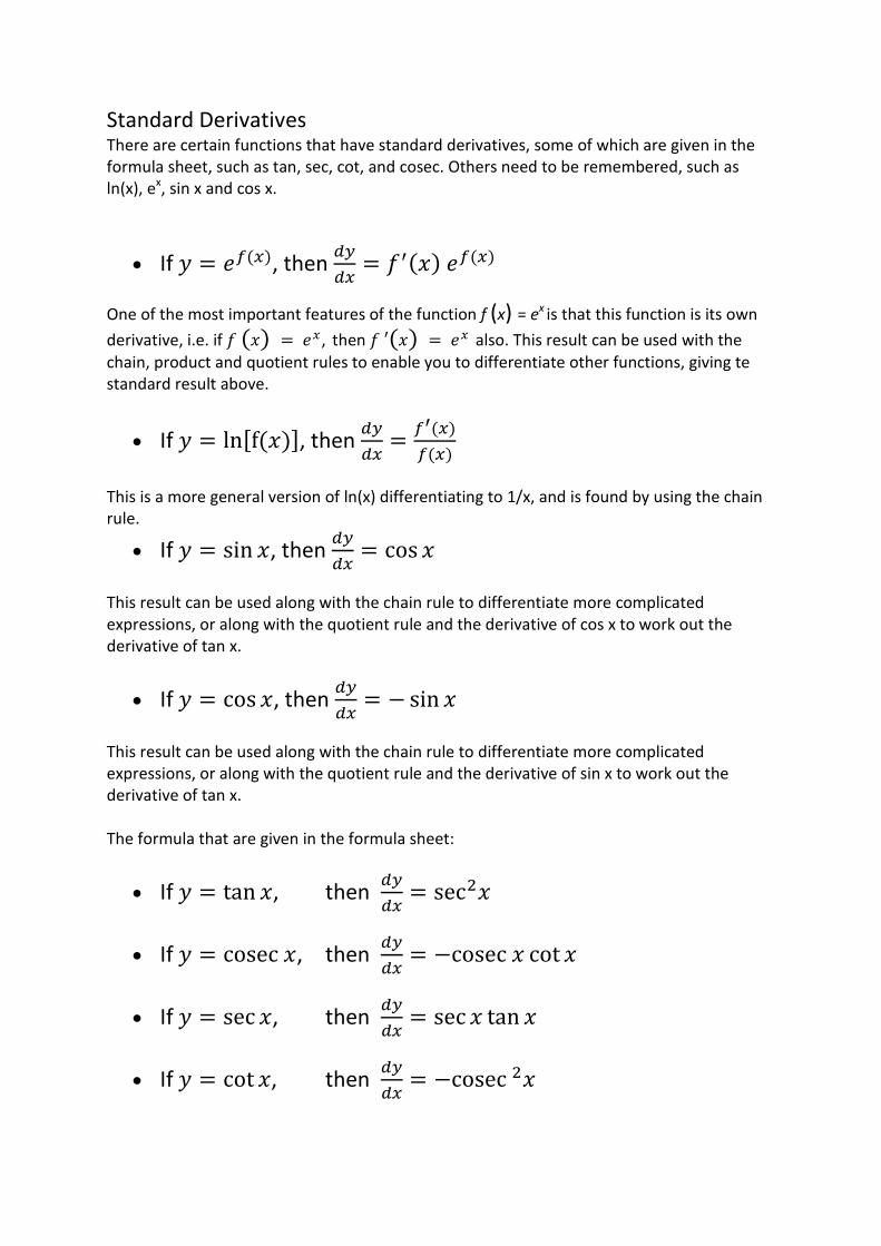
Standard Derivatives There are certain functions that have standard derivatives, some of which are given in the formula sheet, such as tan, sec, cot, and cosec. Others need to be remembered, such as ln(x), ex, sin x and cos x.

• If 𝑦 = 𝑒𝑓(𝑥), then 𝑑𝑦𝑑𝑥

= 𝑓′(𝑥) 𝑒𝑓(𝑥)

One of the most important features of the function f (x) = ex is that this function is its own

derivative, i.e. if 𝑓 (𝑥) = 𝑒𝑥, then 𝑓 ′(𝑥) = 𝑒𝑥 also. This result can be used with the chain, product and quotient rules to enable you to differentiate other functions, giving te standard result above.

• If 𝑦 = ln[f (𝑥)], then 𝑑𝑦𝑑𝑥

= 𝑓′(𝑥)𝑓(𝑥)

This is a more general version of ln(x) differentiating to 1/x, and is found by using the chain rule.

• If 𝑦 = sin 𝑥, then 𝑑𝑦𝑑𝑥

= cos 𝑥 This result can be used along with the chain rule to differentiate more complicated expressions, or along with the quotient rule and the derivative of cos x to work out the derivative of tan x.

• If 𝑦 = cos 𝑥, then 𝑑𝑦𝑑𝑥

= − sin 𝑥 This result can be used along with the chain rule to differentiate more complicated expressions, or along with the quotient rule and the derivative of sin x to work out the derivative of tan x. The formula that are given in the formula sheet:

• If 𝑦 = tan 𝑥, then 𝑑𝑦𝑑𝑥

= sec2𝑥

• If 𝑦 = cosec 𝑥, then 𝑑𝑦𝑑𝑥

= −cosec 𝑥 cot 𝑥

• If 𝑦 = sec 𝑥, then 𝑑𝑦𝑑𝑥

= sec 𝑥 tan 𝑥

• If 𝑦 = cot 𝑥, then 𝑑𝑦𝑑𝑥

= −cosec 2𝑥