ALGEBRAIC DEFORMATION OF A MONOIDAL CATEGORY by TEJ B. SHRESTHA B

ALGEBRAIC DEFORMATION OF A MONOIDAL CATEGORY

by

TEJ B. SHRESTHA

B.Sc., Tribhuvan University, Nepal, 1988

M.Sc., Tribhuvan University, Nepal, 1991

M.S., Kansas State University, 2005


AN ABSTRACT OF A DISSERTATION

submitted in partial fulfillment of the

requirements for the degree

DOCTOR OF PHILOSOPHY

Department of Mathematics

College of Arts and Sciences

KANSAS STATE UNIVERSITY

Manhattan, Kansas

2010

Abstract

This dissertation begins the development of the deformation theorem of monoidal cat-

egories which accounts for the function that all arrow-valued operations, composition, the

arrow part of the monoidal product, and structural natural transformation are deformed.

The first chapter is review of algebra deformation theory. It includes the Hochschild complex

of an algebra, Gerstenhaber’s deformation theory of rings and algebras, Yetter’s deformation

theory of a monoidal category, Gerstenhaber and Schack’s bialgebra deformation theory and

Markl and Shnider’s deformation theory for Drinfel’d algebras.

The second chapter examines deformations of a small k-linear monoidal category. It ex-

amines deformations beginning with a naive computational approach to discover that as

in Markl and Shnider’s theory for Drinfel’d algebras, deformations of monoidal categories

are governed by the cohomology of a multicomplex. The standard results concerning first

order deformations are established. Obstructions are shown to be cocycles in the special

case of strict monoidal categories when one of composition or tensor or the associator is left

undeformed.

At the end there is a brief conclusion with conjectures.

ALGEBRAIC DEFORMATION OF A MONOIDAL CATEGORY

by

TEJ B SHRESTHA

B.Sc., Tribhuvan University, Nepal, 1988

M.Sc., Tribhuvan University, Nepal, 1991



A DISSERTATION

submitted in partial fulfillment of the

requirements for the degree

DOCTOR OF PHILOSOPHY

Department of Mathematics

College of Arts and Sciences

KANSAS STATE UNIVERSITY

Manhattan, Kansas

2010

Approved by:

Major ProfessorDavid N Yetter

Copyright

Tej B Shrestha

2010

Abstract

This dissertation begins the development of the deformation theorem of monoidal cat-

egories which accounts for the function that all arrow-valued operations, composition, the

arrow part of the monoidal product, and structural natural transformation are deformed.

The first chapter is review of algebra deformation theory. It includes the Hochschild complex

of an algebra, Gerstenhaber’s deformation theory of rings and algebras, Yetter’s deformation

theory of a monoidal category, Gerstenhaber and Schack’s bialgebra deformation theory and

Markl and Shnider’s deformation theory for Drinfel’d algebras.

The second chapter examines deformations of a small k-linear monoidal category. It ex-

amines deformations beginning with a naive computational approach to discover that as

in Markl and Shnider’s theory for Drinfel’d algebras, deformations of monoidal categories

are governed by the cohomology of a multicomplex. The standard results concerning first

order deformations are established. Obstructions are shown to be cocycles in the special

case of strict monoidal categories when one of composition or tensor or the associator is left

undeformed.

At the end there is a brief conclusion with conjectures.

Table of Contents

Table of Contents vi

Acknowledgements vii

Dedication viii

1 Introduction 11.1 The Hochschild Homology and Cohomology of an Associative Unital Algebra 21.2 Deformation of Rings and Algebras . . . . . . . . . . . . . . . . . . . . . . . 31.3 Gerstenhaber and Schack’s Double Complex . . . . . . . . . . . . . . . . . . 101.4 The Hochschild Cohomology of k-linear Categories . . . . . . . . . . . . . . 101.5 Drinfel’d Algebra Deformations . . . . . . . . . . . . . . . . . . . . . . . . . 111.6 Yetter’s Cohomology of a Monoidal Category . . . . . . . . . . . . . . . . . . 14

1.6.1 Deformation of Monoidal Structure Maps . . . . . . . . . . . . . . . . 221.6.2 Deformation complexes of monoidal structure maps . . . . . . . . . . 23

2 Deformation of Monoidal Categories 252.0.3 Obstructions to deformation of a k-linear monoidal category . . . . . 382.0.4 Obstruction to deformation of the associativity of composition . . . . 392.0.5 Obstruction to deformation of compatibility between composition and

tensor . . . . . . . . . . . . . . . . . . . . . . . . . . . . . . . . . . . 402.0.6 Obstruction to deformation of naturality of associator . . . . . . . . . 412.0.7 Obstruction to deformation of pentagon condition . . . . . . . . . . . 41

2.1 Obstructions are Cocycles . . . . . . . . . . . . . . . . . . . . . . . . . . . . 422.1.1 Deforming one Structure at a Time . . . . . . . . . . . . . . . . . . . 422.1.2 Deforming two Structures at a Time . . . . . . . . . . . . . . . . . . 53

2.2 A Geometrical Approach to Simplify Messy Calculations . . . . . . . . . . . 642.3 Conclusion . . . . . . . . . . . . . . . . . . . . . . . . . . . . . . . . . . . . . 83

Bibliography 85

A Appendix: Some hand calculations 86

vi

Acknowledgments

I would like to express my special thanks to major professor, Dr. David N Yetter. With-

out his kind continuous guidance and help, this work would have not been completed. I got

support from him to work more than I expected. I am indebt to him for all my life from

the bottom of my heart.

I would like to thank to all other my committee members, Dr. Victor Torchin, Dr. Louis

Crane, Dr. Larry Weaver and outside chair Dr. Mitchell L Neilsen.

I would also like to thank all the faculty members and staff of the Mathematics Depart-

ment at Kansas State University, Kansas. I appreciate easy reachable environment of this

department. I would never forget such an environment in my future career.

At last but not least, I would like to thank all of my colleagues and the students of the

Mathematics Department at K-State whose help and support eased all my hard times.

vii

Dedication

To my parents, mother Ratnamaya, late father

Karnabahadur and to my son, Saurav

viii

Chapter 1

Introduction

A mathematical object may admit many additional structures of a given type. For instance,

an even dimensional manifold may admit many complex structures; a vector space may

admit many algebraic structures; a category may admit many monoidal structures.

Classifying these structures up to some relevant notion of equivalence, analytic equivalence,

isomorphism, or monoidal equivalence in the examples given is often a difficult problem.

Deformation theory or properly, infinitesimal deformation theory contributes to the solution

by classifying structures arbitrarily close to a given structure in the sense of lying in formal

infinitesimal neighborhoods of various orders.

The original deformation theory of Froelicher-Nijenhuis-Kodaira-Spencer dealt with ana-

lytic structures on manifolds. An analogous theory due to Gerstenhaber1,2 dealt with

deformation of associative rings and algebras. In both theories, the first order deformations

are classified by a certain cohomology group, while obstructions to extending a deformation

to higher order are cohomology classes of one higher cohomological dimension. Later, Ger-

stenhaber’s deformation theory for associative algebra was extended to Lie algebra by Nijen-

huis and Richardson. Gerstenhaber observed that the first Hochschild3 cohomology group

H1(A,A) of an algebra, A, classifies all the infinitesimal deformations of automorphisms of

1

A. Similarly the second Hochschild cohomology group H2(A,A) of the algebra A classifies

deformations (of the multiplication) of the algebra A, in particular, if H2(A,A) = 0, A ad-

mits no deformations and is termed ‘rigid’. Fox4 provided some examples of deformation of

associative algebra with graphs and obstruction computations. Gerstenhaber’s deformation

theory of algebra was extended to associative, coassociative bialgebras by Gerstenhaber and

Schack5[1992]. They showed that Hochschild complex of an associative algebra and the dual

to Hochschild complex for a coassociative coalgebra, the Cartier complex6[1956], are com-

patible in a way which allows construction of a double complex (the Hochschild complex in

one direction and the Cartier on the other direction). Gerstenhaber and Schack’s deforma-

tion theory for bialgebras was extended to Drinfel’d algebras by Markl and Shnider7[1996].

The extension, of compatibility condition between the Hoschschild and Cartier differentials

failed and the deformations were governed not by a double complex but by a multicom-

plex. This work is an extension of Gerstenhaber and Schack’s compatibility condition of

two complexes to the Hochschild complex8 for k−linear category and Yetter’s complex9 for

a monoidal category.

We review the main parts of algebraic deformation theory historically with some proofs

to explain the expected form of our own results.

1.1 The Hochschild Homology and Cohomology of an

Associative Unital Algebra

Let k be a field and A be a k-algebra, M be an A-A bimodule. We obtain a simplicial

k-module M ⊗ A⊗∗ with [n]→M ⊗ A⊗n (M ⊗ A⊗0 = M) by defining

∂i(m⊗ a1 ⊗ ...⊗ an) =

ma1 ⊗ ...⊗ an if i = 0

m⊗ ...⊗ aiai+1 ⊗ ...⊗ an if 0 < i < nanm⊗ a1 ⊗ ...⊗ an−1 if i = n

σi(m⊗ a1 ⊗ ...⊗ an) = m⊗ a1 ⊗ ...⊗ ai ⊗ 1⊗ ai+1 ⊗ ...⊗ an

2

for all ai ∈ A,m ∈M where both ∂i and σi are multilinear. So the relations are well-defined

and the required identities are readily verified for the simplicial complex. That is,

0←M∂0−∂1=d1← M ⊗ A d2←M ⊗ A⊗2 d3←M ⊗ A⊗3 d4← · · ·

is a simplicial complex. Similarly [n]→ Homk(A⊗n,M) with

(∂iφ)(a0, a1, ..., an) =

a0φ(a1, ..., an) if i = 0

φ(a0, ..., aiai+1, ..., an) if 0 < i < nφ(a0, a1, ..., an−1) if i = n

(σiφ)(a1, ..., an) = φ(a1, ..., ai, 1, ai+1, ..., an).

Where dn =∑n

i=1(−1)i∂i and dn =∑n

i=1(−1)i∂i.

The nth homology of the former complex is

Hn(A,M) = πn(M ⊗ A⊗∗) = HnC(M ⊗ A⊗∗)

and is called the Hochschild homology of algebra A with coefficients in M and the nth co-

homology of later cocomplex is denoted by

Hn(A,M) = πnHomk(A⊗∗,M) = HnC(Homk(A

⊗∗,M)),

and is called the Hochschild cohomology of algebra A with coefficients in M . In the defor-

mation theory of algebras, one considers the Hochschild cohomology with coefficients in A

itself.

1.2 Deformation of Rings and Algebras

Definition 1.2.1. Let A be an associative algebra over a field k and V be the underlying

vector space of A. Let k[ε]/〈εn〉 = R and VR = V ⊗k R. Then any bilinear function f :

V × V → V can be extended to f : VR × VR → VR. Let f =∑

i f(i)εi, f (0) = f .

3

In particular, if f is a multiplication, we can write f(a, b) = a ∗ b simply= ab, f = ∗ and

a∗b = ab + µ(1)(a, b)ε + µ(2)(a, b)ε2 + · · · . If ∗ is associative, we want ∗ also to be an

associative. Thus we need to have

(a∗b)∗c = a∗(b∗c)

which implies

∑i+j=n0≤i,j

[µ(i)(µ(j)(a, b), c)− µ(i)(a, µ(j)(b, c))] = 0 for n ≥ 0 (1.1)

For n = 0, it is just the associativity of old multiplication of algebra. If n = 1, it is

aµ(1)(b, c)− µ(1)(ab, c) + µ(1)(a, bc)− µ(1)(a, b)c = 0,

which is precisely the condition that µ(1) be the Hochschild 2-cocycle of the complex on A

with coefficient in A. That is, an infinitesimal of deformation of multiplication of an algebra

A is a Hochschild 2-cocycle. If A was commutative and we require commutativity of the

deformed multiplication, then we have another relation

a∗b = b∗a implies µ(i)(a, b) = µ(i)(b, a) ∀i.

A finite deformation of multiplication is of 1-parameter family and the infinitesimal of it is

in Z2(A,A). But for any f ∈ Z2(A,A), it is not necessary that f is to be an infinitesimal of

1-parameter family. If it is such, then Gerstenhaber termed this as integrable. This implies

that the existence of infinite sequence of relations which may be interpreted as the vanishing

of “obstructions” to the integration of f .

Definition 1.2.2. (The Trivial Deformation): A deformation Ft : VR × VR → VR of an

associative algebra, V is trivial if Ft(a, b) = ab+∑

i µ(i)(a, b)εi and µ(i) = 0 ∀i > 0.

4

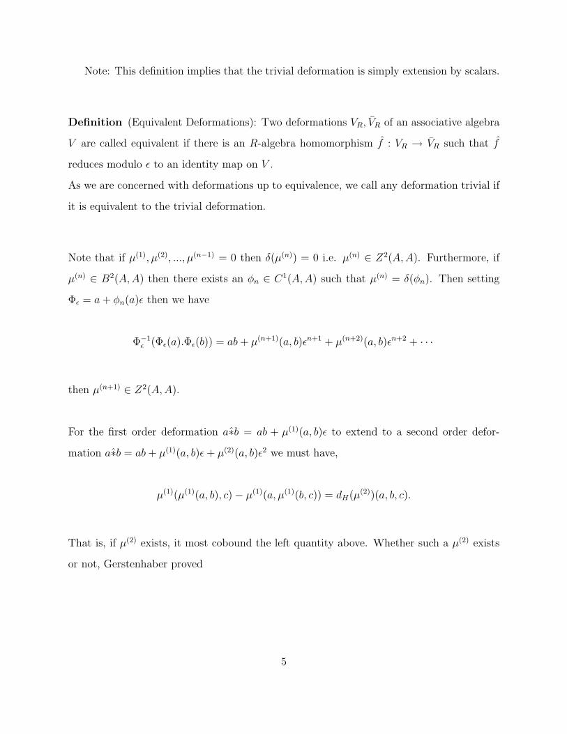
Note: This definition implies that the trivial deformation is simply extension by scalars.

Definition (Equivalent Deformations): Two deformations VR, VR of an associative algebra

V are called equivalent if there is an R-algebra homomorphism f : VR → VR such that f

reduces modulo ε to an identity map on V .

As we are concerned with deformations up to equivalence, we call any deformation trivial if

it is equivalent to the trivial deformation.

Note that if µ(1), µ(2), ..., µ(n−1) = 0 then δ(µ(n)) = 0 i.e. µ(n) ∈ Z2(A,A). Furthermore, if

µ(n) ∈ B2(A,A) then there exists an φn ∈ C1(A,A) such that µ(n) = δ(φn). Then setting

Φε = a+ φn(a)ε then we have

Φ−1ε (Φε(a).Φε(b)) = ab+ µ(n+1)(a, b)εn+1 + µ(n+2)(a, b)εn+2 + · · ·

then µ(n+1) ∈ Z2(A,A).

For the first order deformation a∗b = ab + µ(1)(a, b)ε to extend to a second order defor-

mation a∗b = ab+ µ(1)(a, b)ε+ µ(2)(a, b)ε2 we must have,

µ(1)(µ(1)(a, b), c)− µ(1)(a, µ(1)(b, c)) = dH(µ(2))(a, b, c).

That is, if µ(2) exists, it most cobound the left quantity above. Whether such a µ(2) exists

or not, Gerstenhaber proved

5

Proposition 1.2.3 (Gerstenhaber). The quantity µ(1)(µ(1)(a, b), c) − µ(1)(a, µ(1)(b, c)) =

ω(1)(a, b, c) is a 3-cocycle.

Proof. δ(ω(1))(a, b, c, d)

= aω(1)(b, c, d)− ω(1)(ab, c, d) + ω(1)(a, bc, d)− ω(1)(a, b, cd) + ω(1)(a, b, c)d

= aµ(1)(µ(1)(b, c), d)− aµ(1)(b, µ(1)(c, d))− µ(1)(µ(1)(ab, c), d) + µ(1)(ab, µ(1)(c, d))

+ µ(1)(µ(1)(a, bc), d)− µ(1)(a, µ(1)(bc, d))− µ(1)(µ(1)(a, b), cd) + µ(1)(a, µ(1)(b, cd))

+ µ(1)(µ(1)(a, b), c)d− µ(1)(a, µ(1)(b, c))d

= aµ(1)(µ(1)(b, c), d)

− aµ(1)(b, µ(1)(c, d)) + µ(1)(ab, µ(1)(c, d))− µ(1)(µ(1)(ab, c), d) + µ(1)(µ(1)(a, bc), d)

− µ(1)(a, µ(1)(bc, d)) + µ(1)(a, µ(1)(b, cd))− µ(1)(µ(1)(a, b), cd) + µ(1)(µ(1)(a, b), c)d

− µ(1)(a, µ(1)(b, c))d

Linearity= aµ(1)(µ(1)(b, c), d)

− µ(1)(a, b)µ(1)(c, d) + µ(1)(a, bµ(1)(c, d))− µ(1)(aµ(1)(b, c), d) + µ(1)(µ(1)(a, b)c, d)

− µ(1)(a, bµ(1)(c, d)) + µ(1)(a, µ(1)(b, c)d) + µ(1)(a, b)µ(1)(c, d)− µ(1)(µ(1)(a, b)c, d)

− µ(1)(a, µ(1)(b, c))d

= 0

The quantity ω(1) obstructs extension of a first order deformation to the second order

deformation. If this is zero as a cohomology class, then we can extend the deformation to

second order as

a∗b = a ∗ b+ µ(1)(a, b)ε+ µ(2)(a, b)ε2

6

otherwise we can not. The general obstruction is

∑i+j=n+1

0≤i,j

[µ(i)(µ(j)(a, b), c)− µ(i)(a, µ(j)(b, c))] = ω(n)(a, b, c).

Theorem 1.2.4. The obstruction ω(n) is 3-cocycle for all n.

Proof. We have

−d(µ(k))(a, b, c) = ω(k−1)(a, b, c) =∑i+j=k

0≤i,j≤k−1

[µ(i)(µ(j)(a, b), c)− µ(i)(a, µ(j)(b, c))], k ≤ n

Then

d(ω(n))(a, b, c, d) = aω(n)(b, c, d)− ω(n)(ab, c, d) + ω(n)(a, bc, d)− ω(n)(a, b, cd) + ω(n)(a, b, c)d

=∑

i+j=n+10≤i,j≤n

[aµ(i)(µ(j)(b, c), d)− aµ(i)(b, µ(j)(c, d))− µ(i)(µ(j)(ab, c), d) + µ(i)(ab, µ(j)(c, d))

+ µ(i)(µ(j)(a, bc), d)− µ(i)(a, µ(j)(bc, d))− µ(i)(µ(j)(a, b), cd) + µ(i)(a, µ(j)(b, cd))

+ µ(i)(µ(j)(a, b), c)d− µ(i)(a, µ(j)(b, c))d]

=∑

i+j=n+10≤i,j≤n

[aµ(i)(µ(j)(b, c), d)− aµ(i)(b, µ(j)(c, d))− µ(i)(µ(j)(ab, c)− µ(j)(a, bc), d)

+ µ(i)(ab, µ(j)(c, d))− µ(i)(a, µ(j)(bc, d)− µ(j)(b, cd))− µ(i)(µ(j)(a, b), cd)

+ µ(i)(µ(j)(a, b), c)d− µ(i)(a, µ(j)(b, c))d]

=∑

i+j=n+10≤i,j≤n

[aµ(i)(µ(j)(b, c), d)− aµ(i)(b, µ(j)(c, d))

− µ(i)(aµ(j)(b, c)− µ(j)(a, b)c+∑

p+q=j0≤p,q<j

[µ(p)(µ(q)(a, b), c)− µ(p)(a, µ(q)(b, c))], d)

− µ(i)(a, bµ(j)(c, d)− µ(j)(b, c)d+∑

p+q=j0≤p,q<j

[µ(p)(µ(q)(b, c), d)− µ(p)(b, µ(q)(c, d))])

+ µ(i)(ab, µ(j)(c, d))− µ(i)(µ(j)(a, b), cd) + µ(i)(µ(j)(a, b), c)d− µ(i)(a, µ(j)(b, c))d]

=∑

i+j=n+10≤i,j≤n

[aµ(i)(µ(j)(b, c), d)− µ(i)(aµ(j)(b, c), d) + µ(i)(a, µ(j)(b, c)d)− µ(i)(a, µ(j)(b, c))d

7

− aµ(i)(b, µ(j)(c, d)) + µ(i)(ab, µ(j)(c, d))− µ(i)(a, bµ(j)(c, d)) + µ(i)(a, b)µ(j)(c, d)

− µ(i)(a, b)µ(j)(c, d) + µ(i)(µ(j)(a, b)c, d)− µ(i)(µ(j)(a, b), cd) + µ(i)(µ(j)(a, b), c)d

− µ(i)(∑

p+q=j0≤p,q<j


− µ(i)(a,∑

p+q=j0≤p,q<j

[µ(p)(µ(q)(b, c), d)− µ(p)(b, µ(q)(c, d))])]

=∑

i+j=n+10≤i,j≤n

[−∑

p+q=j0≤p,q<j

[µ(p)(µ(q)(a, µ(j)(b, c)), d)− µ(p)(a, µ(q)(µ(j)(b, c), d))]

+∑

p+q=j0≤p,q<j

[µ(p)(µ(q)(a, b), µ(j)(c, d))− µ(p)(a, µ(q)(b, µ(j)(c, d)))]

+∑

p+q=j0≤p,q<j

[µ(p)(µ(q)(µ(j)(a, b), c), d)− µ(p)(µ(j)(a, b), µ(q)(c, d))]

− µ(i)(∑

p+q=j0≤p,q<j


− µ(i)(a,∑

p+q=j0≤p,q<j

[µ(p)(µ(q)(b, c), d)− µ(p)(b, µ(q)(c, d))])]

=∑

i+j=n+10≤i,j≤n

∑p+q=j

0≤p,q<j[−µ(p)(µ(q)(a, µ(j)(b, c)), d)− µ(p)(a, µ(q)(µ(j)(b, c), d))

+ µ(p)(µ(q)(a, b), µ(j)(c, d))− µ(p)(a, µ(q)(b, µ(j)(c, d)))

+ µ(p)(µ(q)(µ(j)(a, b), c), d)− µ(p)(µ(j)(a, b), µ(q)(c, d))

− µ(i)(µ(p)(µ(q)(a, b), c)− µ(p)(a, µ(q)(b, c)), d)

− µ(i)(a, µ(p)(µ(q)(b, c), d)− µ(p)(b, µ(q)(c, d)))]

=∑

i+j+k=n+1

0<i,j,k≤n[−µ(i)(µ(j)(a, µ(k)(b, c)), d) + µ(i)(a, µ(j)(µ(k)(b, c), d))

+ µ(i)(µ(j)(a, b), µ(k)(c, d))− µ(i)(a, µ(j)(b, µ(k)(c, d))) + µ(i)(µ(j)(µ(k)(a, b), c), d)

− µ(i)(µ(j)(a, b), µ(k)(c, d))− µ(i)(µ(j)(µ(k)(a, b), c)− µ(j)(a, µ(k)(b, c)), d)

− µ(i)(a, µ(j)(µ(k)(b, c), d)− µ(j)(b, µ(k)(c, d)))]

=∑

i+j+k=n+1

0<i,j,k≤n[µ(i)(µ(j)(a, µ(k)(b, c)), d)− µ(i)(µ(j)(a, b), µ(k)(c, d))

− µ(i)(µ(j)(a, µ(k)(b, c)), d)− µ(i)(µ(j)(a, b), µ(k)(c, d))]

= 0

8

Theorem 1.2.5. (Gerstenhaber) Let µt be a 1-parameter family of deformations of an

algebra A. Then µt is equivalent to a family of µ(i)’s

gε(a, b) = ab+ µ(n+1)(a, b)εn+1 + µ(n+2)(a, b)εn+2 + · · ·

where the first non-vanishing cochain if µ(n) ∈ Z2(A,A) and not cohomologous to zero.

Corollary 1.2.1. If H2(A,A) = 0 then A is rigid.

9

1.3 Gerstenhaber and Schack’s Double Complex

Building on results of Gerstenhaber, Gerstenhaber and Schack[1992] showed that the Hochschild

complex of an associative algebra and the Cartier complex of coassociative coalgebra are

compatible in the sense that

......

......

. . .

Homk(A⊗3, k)

OO

// Homk(A⊗3, A)

dh

OO

// Homk(A⊗3, A⊗2)

OO

// Homk(A⊗3, A⊗3)

OO

// · · ·

Homk(A⊗2, k)

OO

// Homk(A⊗2, A)

dh

OO

// Homk(A⊗2, A⊗2)

OO

// Homk(A⊗2, A⊗3)

OO

// · · ·

Homk(A, k)

OO

dc // Homk(A,A)

dh

OO

dc // Homk(A,A⊗2)

OO

dc // Homk(A,A⊗3)

OO

dc // · · ·

Homk(k, k)

OO

// Homk(k,A)

dh

OO

// Homk(k,A⊗2)

OO

// Homk(k,A⊗3)

OO

// · · ·

is a double complex where the underline of a ⊗ indicates the imposition of the obvious

induced module structure and the overline indicates the imposition of the obvious induced

comodule structure.

1.4 The Hochschild Cohomology of k-linear Categories

There is a long-known a folk-theorem10 that generalizes Gerstenhaber’s results from k-

algebras to small k-linear categories.

10

Following Yetter, we make,

Definition 1.4.1. If C and D are k−linear categories, the Hochschild complex11 of parallel

functor F,G : C → D has cochain groups given by

Xn(F,G) :=∏

x0,x1,...,xnHomk(C(x0, x1)⊗ ...⊗ C(xn−1, xn),D(F (x0), G(xn)))

with the coboundary,

dY (ψ)(f0 ⊗ ...⊗ fn) = F (f0)⊗ ψ(f1 ⊗ ...⊗ fn) +∑n

i=1 ψ(f1 ⊗ ...⊗ fi−1fi ⊗ ...⊗ fn)

+ (−1)n+1ψ(f0 ⊗ ...⊗ fn−1)⊗G(fn).

Then d2Y = 0.

The Folk theorem then can be stated precisely as:

Theorem 1.4.2 (Folk Theorem). For any small k-linear category H2(IdC, IdC) classifies

deformation of (the composition) of C up to equivalence. Moreover obstructions to extensions

of deformations to higher order, given by formulas formally identical to those in Gersten-

haber are 3-cocycles in C•(C) = X•(IdC, IdC).

1.5 Drinfel’d Algebra Deformations

Definition 1.5.1. (Drinfel’d Algebra) An algebra A = (V, .,∆, φ) where (V, .,∆) is an

associative not necessarily coassociative, unital and counital k-algebra, φ is an invertible

element of V ⊗3, and the usual coassociativity property is replaced by quasi-coassociativity:

(1⊗4)4.φ = φ.(4⊗ 1)4 (1.2)

where the ‘.’ is used to indicate the multiplication of A and the induced multiplication on

V ⊗3. Moreover, φ must satisfy

11

(12 ⊗4)(φ).(4⊗ 12)(φ) = (1⊗ φ).(1⊗4⊗ 1)(φ).(φ⊗ 1) (1.3)

1 ∈ V the unit element and 1, the identity map on V , and if ε : V → k, k the base field, is

the counit of coalgebra (V,4) then (ε⊗ 1)4 = (1⊗ ε)4 = 1.

Note that the bialgebra is a Drinfel’d algebra with φ = 1.

Markl and Shnider[1996] extended the Gerstenhaber and Schack[1992] bialgebra deformation

bicomplex to a Drinfel’d algebra deformation multicomplex. Because of the non-associativity

nature of Drinfel’d algebra, the vertical and horizontal differential do not cancel each other.

This adds significant complication of computation to the interactions among parts of the

deformations and is not easy to handle by hand. The interactions of can not be encoded

in a bicomplex. Markl and Shnider had to introduce additional differentials and used the

term ‘homotopy differentials’. They are not exactly a differential, but are differential up to

homotopy.

Definition 1.5.2. A multicomplex C(•,•) is a bigraded complex with the differentials given by

dj : C(p,q) → C(p+j,q−j+1); q ≥ j ≥ 0

such that if

d =

d0 0 0 · · · od1 d0 0 · · · od2 d1 d0 · · · o...

...... · · ·

...dn−1 dn−2 dn−3 · · · d0

dn dn−1 dn−2 · · · d1

: ⊕ni=1C

(n−i,i) → ⊕n+1i=1 C(n−i,i),

such that d2 = 0.

Markl and Shnider used a geometrical approach and found that Stasheff polytopes pro-

vide descriptions of the complicated differentials using grouping objects by parenthesis [like

12

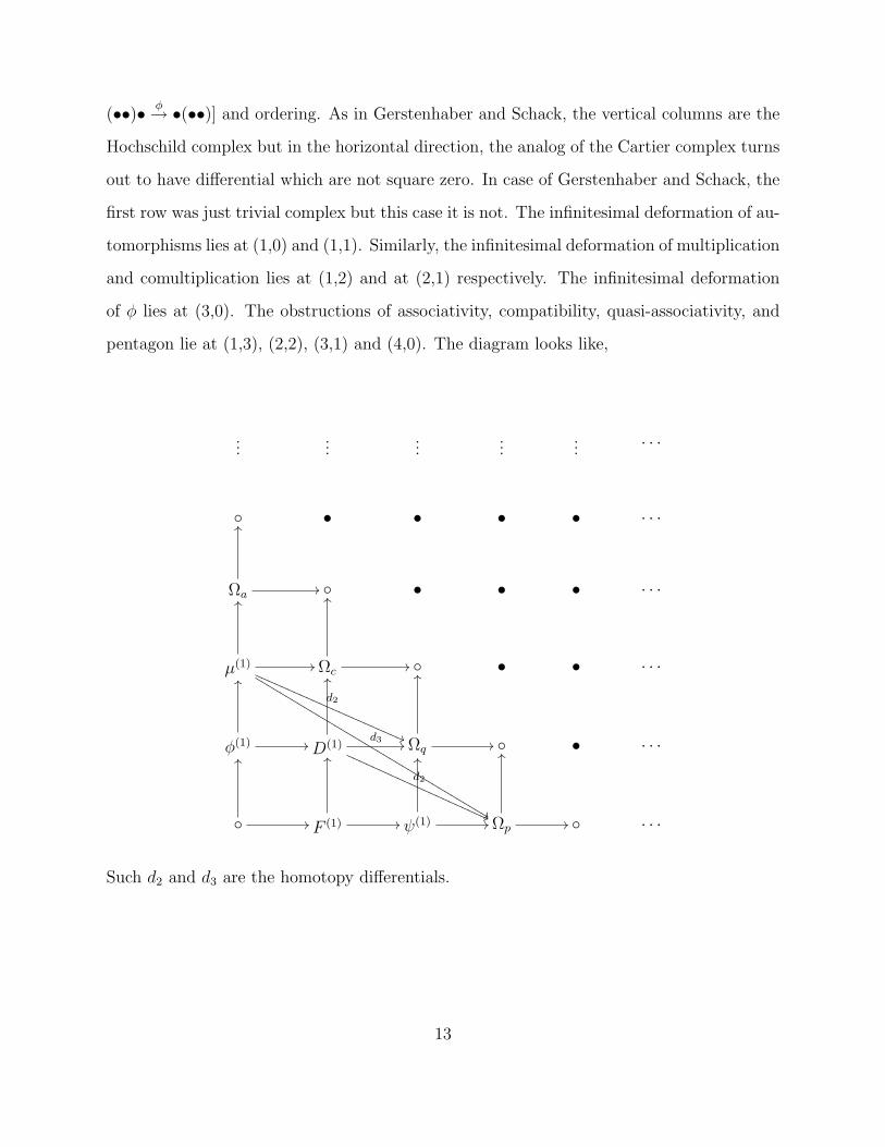
(••)• φ→ •(••)] and ordering. As in Gerstenhaber and Schack, the vertical columns are the

Hochschild complex but in the horizontal direction, the analog of the Cartier complex turns

out to have differential which are not square zero. In case of Gerstenhaber and Schack, the

first row was just trivial complex but this case it is not. The infinitesimal deformation of au-

tomorphisms lies at (1,0) and (1,1). Similarly, the infinitesimal deformation of multiplication

and comultiplication lies at (1,2) and at (2,1) respectively. The infinitesimal deformation

of φ lies at (3,0). The obstructions of associativity, compatibility, quasi-associativity, and

pentagon lie at (1,3), (2,2), (3,1) and (4,0). The diagram looks like,

......

......

... · · ·

• • • • · · ·

Ωa//

OO

• • • · · ·

µ(1) //

OO

d2

((QQQQQQQQQQQQQQQQQQQQQQQ

d3

%%LLLLLLLLLLLLLLLLLLLLLLLLLLLLLLLLLLLLLL Ωc//

OO

• • · · ·

φ(1) //

OO

D(1)

d2

((QQQQQQQQQQQQQQQQQQQQQQ//

OO

Ωq//

OO

• · · ·

//

OO

F (1) //

OO

ψ(1) //

OO

Ωp//

OO

· · ·

Such d2 and d3 are the homotopy differentials.

13

1.6 Yetter’s Cohomology of a Monoidal Category

Following Mac Lane12 we make,

Definition 1.6.1. A graph (also called a “diagram scheme”) is a set O of objects, a set A

of arrows, and two functions Adom //

cod// O. In this graph, the set of composable pairs of arrows

is the set

A×O A = 〈g, f〉|g, f ∈ A and domg = codf,

called the “product over O”.

A small category is a graph with two additional functions

Oid

→ A, A×O A→ A

c 7→ idc, 〈g, f〉 7→ g f

called the identity and composition, such that

dom(id a) = a = cod(id a), dom(g f) = domf, cod(g f) = codg

for all objects a ∈ O and all composable pairs of arrows 〈g, f〉 ∈ A×O A and such that the

associativity and unit axioms hold.

The expression f : X → Y is shorthand for the assertion that f is an arrow in a category,

made clear in context, whose source is the object X and whose target is the object Y .

We let

C(X, Y ) = f : X → Y |f ∈ Arr(C) = HomC(X, Y )

and call these sets “hom-sets”.

14

Definition 1.6.2. For any unital commutative ring R, an R-linear category is a category

whose hom-sets are each equipped with an R-modules structure and in which composition is

R-bilinear.

Definition 1.6.3. R−mod is an R-linear category, where R is a unital commutative rings,

is a R-linear category with objects are R-modules and arrows are R-module homomorphisms.

k − V.S. for k is a field, the category with objects, k-vector spaces, and arrows are k-linear

transformations between vector spaces,is k-linear category.

Definition 1.6.4. (Functor) Let C and D be two categories. A functor F : C → D is an

assignment to every object X of C of an object F (X) of D such that for X, Y, Z ∈ Ob(C),

and to every arrow f of C an arrow F (f) of D, Xf→ Y implies F (X)

F (f)→ F (Y ) and

Xf→ Y

g→ Z implies F (X)F (f)→ F (Y )

F (g)→ F (Z) and that F (fg) = F (f)F (g).

Definition 1.6.5. (Natural Transformation) Let F,G : C → D be two functors from category

C to category D. Then a natural transformation φ from F to G is denoted by φ : F ⇒ G and

is an assignment to each X ∈ Ob(C) of an arrow φX : F (X)→ G(X) in Arr(D) satisfying

φXG(f) = F (f)φY for all f : X → Y in C. That is,

F (X)F (f)

//

φX

F (Y )

φY

G(X)G(f)

// G(Y )

commutes.

If F,G,H : C → D are functors and φ : F ⇒ G, ψ : G ⇒ H are natural transforma-

tions, then

15

F (X)F (f)

//

φX

F (Y )

φY

G(X)G(f)

//

ψX

G(Y )

ψY

H(X)H(f)

// H(f)

for any f : X → Y in C. So φψ : F ⇒ G is a natural transformation.

A natural transformation φ such that each φx is an isomorphism is called a “natural iso-

morphism”.

Definition 1.6.6. (Equivalence of two categories) Let C and D be two categories and if

there exist functors F : C → D and G : D → C and natural isomorphisms φ : FG ⇒ IdC

and ψ : GF ⇒ IdD then we say such a quadruple (F,G, φ, ψ) is called an equivalence of

categories between categories C and D.

Definition 1.6.7. Let C and D be two small categories. Then the product C × D is the

category with objects Ob(C×D) = Ob(C)×Ob(D) and arrows Arr(C×D) = Arr(C)×Arr(D)

and all operations (source, target, identity arrow, and composition) given coordinatewise by

those of C and D.

Definition 1.6.8. (Monoidal Category) A category C is a monoidal category equipped with a

functor ⊗ : C×C → C, an object I, and natural isomorphisms α : ⊗(⊗×1C)⇒ ⊗(1C×⊗), ρ :

⊗I ⇒ 1C, λ : I⊗ ⇒ 1C such that all instances of diagrams of the form

16

(AB)(CD)

αA,B.CD

&&MMMMMMMMMMMMMMMMMMMMMMMM

((AB)C)D

αAB,C,D

88qqqqqqqqqqqqqqqqqqqqqqqq

αA,B,C⊗D

;;;;;;;;;;;;;;;;

A(B(CD))

(A(BC))D αA,BC,D// A((BC)D)

A⊗αB,C,D

AA

and

(A⊗ I)⊗B α //

ρ⊗B

$$HHHHHHHHHHHHHHHHHA⊗ (I ⊗B)

A⊗λ

zzvvvvvvvvvvvvvvvvv

A⊗B ,

commute.The commutativity of these diagrams are called the coherence conditions for a

monoidal category C. In the case of R-linear categories we require that the maps induced on

hom-sets by ⊗ be R-bilinear.

Example 1.6.9. (Sets,×, ∗, α, ρ, λ) where ×=cartesian product

*=singleton set

α : ((a, b), c) 7→ (a, (b, c))

ρ : (a, ∗) 7→ a and λ : (∗, a) 7→ a

17

and the naturality for ρ is

(a, ∗) ρ//

f

a

f

(f(a), ∗) ρ// f(a).

Example 1.6.10. (sets,⊔, φ, α, λ, ρ)9, where φ is the empty set, is monoidal category.

Definition 1.6.11. 9 A tangle is an embedding T : X → I3 where I = [0, 1] of a 1-manifold

with boundary into the rectangular solid I3 satisfying

T (∂X) = T (X)⋂

∂I3 = T (X)⋂

(I2 × 0, 1).

Example 1.6.12. (Tang,⊗, I, α, λ, ρ), where I is the empty tangle, and ⊗ is defined as: for

two tangles T1, T2, T1⊗T2 has as underlying 1- manifold the disjoint union of the underlying

1-manifold of T1 and T2. T1 ⊗ T2 is then the mapping of this 1-manifold the composition of

T1

∐T2 with the map γ : I3

∐I3 → I3 given by

(x, y, z) 7→ (x/2, y, z) for elements of the first summand, and

(x, y, z) 7→ ((x+ 1)/2, y, z) for elements of the second summand.

Example 1.6.13. Let k be a field. Then (H − mod,⊗ = ⊗k, k, α, λ, ρ) where H is a

bialgebra. This is a monoidal category.

Example 1.6.14. Let k be a field. Then (R−mod,⊗ = ⊗R, R, α, λ, ρ) where R is a unital

commutative algebra. This is a R-linear monoidal category.

Example 1.6.15. Let k be a field. Then (k − v.s.,⊗ = ⊗k, k, α, λ, ρ). This category is a

k-linear monoidal category.

Definition 1.6.16. (Fusion Category)13 By a fusion category C over a field k is a k-linear

semisimple rigid tensor category with finitely many simple objects and finite dimensional

18

hom-sets, and the hom-set C(I, I), which is necessarily a k-algebra under composition, is

isomorphic to k.

Example 1.6.17. Any fusion category is a k-linear monoidal category.

Definition 1.6.18 (Strong Monoidal Functor). : Let F : C → D be a functor from monoidal

category C to monoidal category D equipped with a natural isomorphism

F : F (.)⊗ F (.)→ F (.⊗ .) and an isomorphism FI : I → F (I)

satisfying

F ((A⊗B)⊗ C)F (α)

// F (A⊗ (B⊗))

F (A⊗B)⊗ F (C)

FA⊗B,C

OO

F (A)⊗ F (B ⊗ C)

FA,B⊗C

OO

(F (A)⊗ F (B))⊗ F (C)

FA,B⊗F (C)

OO

β// F (A)⊗ (F (B)⊗ F (C))

F (A)⊗FB,C

OO

F (A) F (A⊗ I)F (ρA)

oo F (A) F (I ⊗ A)F (λA)

oo

F (A)⊗ I⊗

ρF (A)

OO

F (A)⊗ F (I)F (A)⊗FIoo

FA,I

OO

I ⊗ F (A)

λF (A)

OO

F (I)⊗ F (A)FI⊗F (A)oo

FI,A

OO

is called strong monoidal functor.

A monoidal functor F : C → D is called strict if F is the identity transformation and FI

is an identity arrow.

19

Definition 1.6.19. (Monoidal natural transformation): A monoidal natural transformation

is a natural transformation φ : F ⇒ G between two monoidal functors which satisfies

FA,B(φA⊗B) = φA ⊗ φB(GA,B)

and FI = GI(φI).

Example 1.6.20. For any k-bialgebra A, the functor from A-mod to k-vector space is a

strict monoidal functor.

Example 1.6.21. The free group functor

F : (Sets,⊔, λ, ρ, α)→ (Grps, ∗, λ, ρ, α)

equipped with structure maps induced by inclusions of generators and universal property of

free groups is a strong monoidal functor.

Example 1.6.22. For a Drinfel’d algebra R, the forgetful functor F : R− bimod→ k−v.s.

is a strong monoidal functor but not strict monoidal functor, unless R is a bialgebra, in

which case it is strict.

Definition 1.6.23. (Monoidal Equivalence) A monoidal equivalence between two monoidal

categories C and D is an equivalence of categories in which the functors F : C → D and G :

D → C are equipped with the structure of monoidal functors, and the natural isomorphisms

φ : FG⇒ IdC and ψ : GF ⇒ IdD are both monoidal natural transformations. If there exists

a monoidal equivalence between C and D, we say that C and D are monoidally equivalent.

Definition 1.6.24. A formal diagram in the theory of monoidal categories is a diagram in

the free monoidal category on S for some set S.

20

Theorem 1.6.25. (Mac Lane’s Coherence Theorem 1st version)12: Every formal diagram

in the theory of monoidal categories commutes. Consequently, any diagram which is the

image of formal diagram under a (strict Monoidal) functor commutes.

(2nd version): Every monoidal category is monoidally equivalent to a strict monoidal cate-

gory.

The following notion due to Yetter embodies Mac Lane’s coherence theorem in a natural,

useful way,

Definition 1.6.26. A prolongation of an arrow f in a monoidal category is a map obtained

by iterated monoidal product of f with identity maps of various objects.

Definition 1.6.27. (Padded composition): Given a monoidal category C and a sequence of

maps f1, f2, ..., fn ∈ C such that source of fi+1 is isomorphic to the target of fi by a compo-

sitions of prolongations of structure maps, we denote by df1, f2, ...fne,

the composition a0f1a1f2a2...an−1fnan where ai are composition of prolongations of structure

maps and

1. source of a0 is reduced and completely left parenthesized

2. The target of an is reduced and completely right parenthesized

3. Composite is well-defined.

Padded composition has the following properties:

1. df1, ..., fne = df1, ..., fiedfi+1, ..., fne

2. df1, ..., g ⊗ I, ..., fne = df1, ..., g, ..., fne = df1, ..., I ⊗ g, ..., fne

21

3. df1, ..., fne = df1, ..., fi−1, dfi, fi+1, ..., fle, ..., fne

4. df1, ..., g ⊗ h, ..., fne = df1, ..., dge ⊗ h, ..., fne = df1, ..., g ⊗ dhe, ..., fne

1.6.1 Deformation of Monoidal Structure Maps

Let C be a k-linear category and A be a k-algebra. We can form a category C ⊗k A = C by

extension of scalars

Ob(C) = Ob(C) HomC(X, Y ) = HomC(X, Y )⊗k A

that is, if f ∈ HomC(X, Y ) and g ∈ HomC(X,Z) then

∑i

fi ⊗ ai∑j

gj ⊗ bj =∑i,j

fiCgjaibj.

If A is a local ring with m as its maximal ideal, then we can extend the composition on

C ⊗A, to a composition on C⊗A, the category whose hom-sets are the m-adic completions

of those of C ⊗ A, by continuity. For A = k[ε]/ < εn+1 >, we denote C ⊗k A = C(n) and if

A = k[|ε|], C⊗A is denoted by C(∞).

Definition 1.6.28. Given a k-linear monoidal category C, an nth order deformation of

the structure maps of the category is a monoidal category structure on C(n) whose struc-

tural functors are the extensions of those of C by bilinearity and whose structural natural

transformations reduce modulo ε to those of C.

Definition 1.6.29. Given a k-linear monoidal category C, a formal deformation of struc-

ture maps of the category is a monoidal structure on C(∞), whose structural functors are the

extensions of those of C by bilinearity and continuity, and whose structural natural trans-

formations modulo ε is those of C.

Definition 1.6.30. (The Trivial Deformation) The deformation of a monoidal category C

whose structural natural transformations are the images of those in C under extension of

22

scalars. It is denoted by C(n)triv(resp. C(∞)

triv ).

Definition 1.6.31. Two deformations of a monoidal category are equivalent if there is

a monoidal equivalence between them whose structural natural isomorphism reduce to the

identity modulo ε. As we are concerned with deformations up to equivalence, we say a

deformation is trivial if it is equivalent to the trivial deformation.

1.6.2 Deformation complexes of monoidal structure maps

Definition 1.6.32. The deformation complex of the structure maps of a monoidal category

(C,⊗, α) is the cochain complex (X•(C), δ) where

Xn(C) = Nat(n⊗,⊗n) and

dY (φ)A0,...,An = dA0 ⊗ φA1,...,Ane+∑

i(−1)idφA0,...,Ai−1⊗Ai,...,Ane+ d(−1)n+1φA0,...,An−1⊗Ane.

Theorem 1.6.1 (Yetter). The first order deformations of a monoidal category C are clas-

sified up to equivalence by H3(C).

Now consider the nth order deformation of associator α which is given by

α =∑n

i=0 α(i)εi α(0) = α.

Then the obstruction to extending to the n+ 1st order deformation is

ω(n)ABCD =

∑i+j=n+1

0<i,j

α(i)A⊗BCDα

(j)ABC⊗D −

∑i+j=n+1

0<i,j

[α(i)ABC ⊗D]α

(j)AB⊗CD[A⊗ α(k)

BCD]

=∑

i+j=n+10<i,j

∂1α(i)∂3α

(j) −∑

i+j=n+10<i,j

∂0α(i)∂2α

(j)∂4α(k)

where ∂0α = A ⊗ αBDC ; ∂1α = αA⊗BCD; ∂2α = αAB⊗CD; ∂3α = αABC⊗D; ∂4α = αABC ⊗ D

that is the operator ∂i means the objects are pre-tensored at ith place. Using this shorthand

notation we can easily see that∑4

i=0(−1)i∂iα(1) = 0, i.e. the first order deformation of

23

associator is a 3-cocycle.

Theorem 1.6.2 (Yetter). For all n, the nth order obstruction is a 4-cocycle. Thus an

(n− 1)th order deformation of a monoidal structure extends to nth order deformation if and

only if the cohomology class [ω(n)] ∈ H4(C) vanishes.

24

Chapter 2

Deformation of Monoidal Categories

Definition 2.0.33. (Deformations of a monoidal category) Let (C,⊗, I, α, ρ, λ) be a k-linear

monoidal category and R be a unital commutative local k-algebra with maximal ideal m.

The deformation of a monoidal category C is an R-linear category C whose objects are those

of C and whose hom-sets are given by C(X, Y ) = C(X, Y )⊗R, where ⊗ denotes the m-

adic completion of the ⊗ over k whose composition, arrow-part of ⊗ and structural natural

isomorphisms reduce modulo m to those of C. We denote by ‘x’, the deformed structure

corresponding to x.

Note: Through out we use the convention that‘.’ denotes the monoidal operation when

it occurs in the argument of any arrow-value operation, e.g. a.f ⊗k denote (a⊗f)⊗k when

we are considering the monoidal product of a and f as the first argument of ⊗.

We consider one parameter deformations, that is the case of R = k[ε]/〈εn+1〉;n ∈ N or

R = k[|ε|]. As in the review of deformation theory in Chapter 1, we call a deformation of

the first sort an nth-order deformation, and of the latter sort a formal deformation.

Definition 2.0.34. Two deformations C and C of C are equivalent if there is an R-linear

monoidal equivalence between them, the arrow part of whose functors and natural isomor-

phisms reduce modulo m to identities.

Proposition 2.0.35. If C and C are nth order or formal deformations of C and (F, F , F1)

is a monoidal functor from C to C such that F, F and F1 reduce to ε to identity functor,

25

identity natural transformation and identity arrow respectively, then C and C are equivalent.

Sketch of proof. F, F , F1 each have inverses by the same calculations that shows that formal

power series with leading coefficients 1 have inverses.

Proposition 2.0.36. An nth order deformation (resp. formal deformation) of a monoidal

category consists of

1. Composition : f g =∑

i µ(i)(f, g)εi, where µ(0)(f, g) = f g = fg(simply).

2. Tensor ⊗: f⊗k =∑

i τ(i)(f, k)εi, where τ (0)(f, k) = f ⊗ g.

3. Associator α: α =∑

i α(i)εi, where α(0) = α.

when the sums are bounded by n (resp. run from 0 to infinity).

Here f and g are composable arrows but f and k are not necessarily composable ones

and i = 1, 2, .... The supper script ‘(0)’ means the base structure.

Proof. It suffices to observe that by linearity (resp. linearity and completeness), it is enough

to specify composition and tensor on the arrows of C.

By a result of Yetter11, any deformation is equivalent to one which preserves identity

arrows;

Lemma 2.0.3. If the identity arrow of C are identity arrows in C, then

µ(i)(1, f) = µ(i)(f, 1) = 0

for all i > 0.

Proof. Since f = 1 f , f = f + µ(1)(1, f)ε+ µ(2)(1, f)ε2 + .... This implies that

µ(i)(1, f) = 0, i > 0.

26

Lemma 2.0.4. τ (i)(1, 1) = 0 for all i > 0.

Proof. The first order compatibility condition for deformations is given by

τ (1)(a, f)b⊗ g − τ(1)(ab, fg) + a⊗ fτ (1)(b, g)

= µ(1)(a, b)⊗ fg − µ(1)(a⊗ f, b⊗ g) + ab⊗ µ(1)(f, g).

This gives τ (1)(1, 1) = 0 if we take a = 1 = f . Taking second order condition and with the

same choices of a and f , we get τ (2)(1, 1) = 0. Similarly, we can see for the other orders.

Consider the case i = 1, i.e. ε2 = 0. That is, first order deformations. Calculation

of the four conditions that must be satisfied for the deformation to be a monoidal category,

and the three condition which must be satisfied for two deformations to be equivalent reveal

a natural cohomological structure.

1. Associativity of composition. That is,

(ab)c = a(bc) where a, b, c are composable arrows. So, the first order condition is,

µ(1)(a, b)c+ µ(1)(ab, c) = µ(1)(a, bc) + aµ(1)(b, c).

⇒ dH(µ(1))(a, b, c) = 0

which means, µ(1) is a Hochschild 2-cocycle on the complex C• where

Cn =∏

x0,...,xn∈Ob(C)

Homk(C(x0, x1)× ...× C(xn−1, xn), C(x0, xn)).

2. Middle four interchange. That is,

A⊗B a⊗f//

ab⊗fg11U ⊗ V b⊗g// X ⊗ Y.

27

which is,

(a⊗ f) (b⊗ g) = (a b)⊗ (f g) : A⊗B → X ⊗ Y. (2.1)

Then, we need

(ab)⊗(f g) = (a⊗f)(b⊗g)

which we call “compatibility” of tensor and composition. The first order terms give us,

µ(1)(a, b)⊗fg+τ (1)(ab, fg)+ab⊗µ(1)(f, g) = τ (1)(a, g)b⊗g+µ(1)(a⊗f, b⊗g)+a⊗fτ (1)(b, g)

which can be written as

a⊗fτ (1)(b, g)−τ (1)(ab, fg)+τ (1)(a, g)b⊗g = ab⊗µ(1)(f, g)−µ(1)(a⊗f, b⊗g)+µ(1)(a, b)⊗fg

⇒ dH(τ (1))

(a fb g

)= dY (µ(1))

(a fb g

).

With this relation, we see an interaction between τ (1) and µ(1), suggesting a double

complex or perhaps a multi-complex, and that the arguments are those of the second

Hochschild cochain group for CC where is Deligne product. Recall that the Deligne

product of two (small) k-linear categories A and B is the k-linear category with objects

Ob(A)× Ob(B) and hom-sets given by Hom((A,B), (A′, B′)) = A(A,A′)⊗ B(B,B′),

with the obvious notions of composition and identity arrow.

28

Here the dY looks like Yetter’s differential, but with arrows, rather than objects as

arguments.

3. Naturality of α.

We have,

αABC : (A⊗B)⊗ C → A⊗ (B ⊗ C). (2.2)

If (A⊗B)⊗ C (a⊗f)⊗k→ (X ⊗ Y )⊗ Z, then we have the naturality square

(A⊗B)⊗ C αABC //

(a⊗f)⊗k

A⊗ (B ⊗ C)

a⊗(f⊗k)

(X ⊗ Y )⊗ Z αXY Z// X ⊗ (Y ⊗ Z)

that is,

αABC [a⊗ (f ⊗ k)] = [(a⊗ f)⊗ k]αXY Z .

If the composition is not deformed, this gives

α(1)ABC [a⊗ (f ⊗ k)] + αABCτ

(1)(a, f ⊗ k) + αABC [a⊗ τ (1)(f ⊗ k)]

= τ (1)(a⊗ f, k)αXY Z + [τ (1)(a, f)⊗ k]αXY Z + [(a⊗ f)⊗ k]α(1)XY Z

which gives,

α(1)ABC [a⊗ (f ⊗ k)]− [(a⊗ f)⊗ k]α

(1)XY Z

+ αABC [a⊗ τ (1)(f ⊗ k)]− [τ (1)(a, f)⊗ k]αXY Z

+ αABC [a⊗ τ (1)(f ⊗ k)]− [τ (1)(a, f)⊗ k]αXY Z = 0.

29

This can be written as

[dH(α(1)) + dY (τ (1))](a, f, k) := [d0(α(1)) + d1(τ (1))](a, f, k) = 0

This follows the pattern of previous result and we can guess with the Hochschild’s

complexes on one direction and on the other with the Yetter’s complexes. Assume the

Hochschild’s complex of composable arrows in the vertical direction and the Yetter’s

complex on the horizontal direction, at this point also Hochschild’s coboundary and

Yetter’s coboundary cancel each other which is required condition for double complex.

However, deforming the composition also, we get

α(1)ABC [a⊗ (f ⊗ k)]− [(a⊗ f)⊗ k]α

(1)XY Z+ αABC [a⊗ τ (1)(f ⊗ k)]

− [τ (1)(a, f)⊗ k]αXY Z + αABC [a⊗ τ (1)(f ⊗ k)]− [τ (1)(a, f)⊗ k]αXY Z

+ µ(1)(αABC , a⊗ (f ⊗ k))− µ(1)((a⊗ f)⊗ k, αXY Z) = 0.

⇒ [d0(α(1) + d1(τ (1))](a, f, k) + d2(µ(1))(a, f, k) = 0,

where d2(µ(1)) inserts an instance of α as one of the arguments in both possible ways.

This shows, if we deform the all of the associator, tensor, and composition, the defor-

mation are not governed by a double complex. It is more than a double complex. We

can expect it will be a multi-complex. According to the input arguments of µ(1), τ (1)

and α(1), and if we use the number of composable arrows involved as y-coordinate with

0 as the composable arrows when objects are the arguments, and number of tensorands

(objects or arrows) as x-coordinate, we can think their position are at (1,2),(2,1) and

(3,0) respectively. The relations we observed above can be pictorially represented as,

30

0

µ(1)

d0

OO

d1 //

d2

((QQQQQQQQQQQQQQQQQQQQQQQ 0

. τ (1)d1

//

d0

OO

0

. . α(1).

d0

OO

4. The pentagon identity.

The condition

[αABC ⊗D]αAB.CD[A⊗ αBCD] = αA.BCDαABC.D, (2.3)

is called the pentagon identity. Again the dot ‘.’ is used denote that objects or arrows

are tensored before being used as arguments. Deforming only associator, we get

dα(1)ABC ⊗De − dα

(1)A.BCDe+ dα(1)

AB.CDe − dα(1)ABC.De+ dA⊗ α(1)

BCDeY etter

=∑4

i=0(−1)i∂iα(1) = 0.

Which is Yetter’s cocycle condition of the Yetter’s complex [at (4,0)]. Similarly, if

we deform the tensor and associator, we get

4∑i=0

(−1)i∂iα(1) + τ (1)(αABC , D) + τ (1)(A,αBCD) = 0.

Deforming composition also, we have

31

d1(α(1)) + τ (1)(αABC , D)αAB.CD[A⊗ αBCD] + [αABC ⊗D]αAB.CDτ(1)(A,αBCD)

+ µ(1)(αABC ⊗D,αAB.CD)[A⊗ αBCD] + µ(1)([αABC ⊗D]αAB.CD, A⊗ αBCD)

− µ(1)(αA.BCD, αABC.D) = 0.

Under Yetter’s notation of padded composition but suppressing de marks, it is read as

d1(α(1)) + τ (1)(αABC , D) + τ (1)(A,αBCD) + µ(1)(αABC ⊗D,αAB.CD)

+ µ(1)([αABC ⊗D]αAB.CD, A⊗ αBCD)− µ(1)(αA.BCD, αABC.D) = 0

which, then

[d1(α(1)) + d2(τ (1)) + d3(µ(1))](A,B,C,D) = 0.

where

d2(τ (1))(A,B,C,D) = dτ (1)(αABC , D)e+ dτ (1)(A,αBCD)e

and

d3(µ(1))(A,B,C,D) = dµ(1)(αABC ⊗D,αAB.CD)e

+ dµ(1)([αABC ⊗D]αAB.CD, A⊗ αBCD)e − dµ(1)(αA.BCD, αABC.D)e.

This fills the another component for the multi-complex

32

0

µ(1)

d2

((QQQQQQQQQQQQQQQQQQQQQQQ d1//

d0

OO

d3

%%LLLLLLLLLLLLLLLLLLLLLLLLLLLLLLLLLLLLL 0

. τ (1)d1

//

d0

OO

d2

((QQQQQQQQQQQQQQQQQQQQQQ 0

. . α(1)

d0

OO

d1// 0.

Theorem 2.0.37. µ(1), τ (1), α(1) give a first order deformation if and only if they col-

lectively are a cocycle in the total complex of a multicomplex with low order differentials

are given by d0 is the Hochschild differential, d1 is the Yetter differential and

(a) d2(µ(1))(a, f, k) = µ(1)(αABC , a⊗ f.k)− µ(1)(a.f ⊗ k, αXY Z)

(b) d3(µ(1))(A,B,C,D) = dµ(1)(αABC ⊗D,αAB.CD)e

+ dµ(1)([αABC ⊗D]αAB.CD, A⊗ αBCD)e − µ(1)(αA.BCD, αABC.D).

(c) d2(τ (1))(A,B,C,D) = dτ (1)(αABC , D)e+ dτ (1)(A,αBCD)e.

Let us now consider the conditions needed for the first order deformations to be equiv-

alent:

5. Composition preservation

F (f g) = F (f) F (g) implies

F (1)(fg) + µ(1)(f, g) = F (1)(f)f + ν(1)(f, g) + fF (1)(g)

33

⇒ dH(F (1))(f ; g) = [ν(1) − µ(1)](f ; g).

6. Natural Transformation

F : F (−⊗−)→ F (−)⊗ F (−) (2.4)

where F : C → D is a functor from monoidal category C to a monoidal category D.

Then the naturality square

F (A⊗B)FA,B

//

F (f⊗k)

F (A)⊗ F (B)F (f)⊗F (k)

F (X ⊗ Y )FX,Y

// F (X)⊗ F (Y )

gives that FA,BF (f)⊗ F (k) = F (f ⊗ k)FX,Y which implies that, if

ˆF = IdC + φ(1)ε, and F = IdC + F (1)ε

φ(1)A,Bf ⊗k+F (1)(f)⊗k+ f ⊗F (1)(k) +ρ(1)(f, k) = F (1)(f ⊗k) + f ⊗kφ(1)

X,Y + τ (1)(f, k)

which is equivalent to say

[d1(F (1)) + d0(φ(1))](f ⊗ k) = τ (1)(f, k)− ρ(1)(f, k).

Then the above picture is extended to,

34

0

µ(1)

d2


d0

OO

d3


F (1)d1

//

d0

OO

τ (1)d1

//

d0

OO

d2

((PPPPPPPPPPPPPPPPPPPPPP 0

. φ(1)

d0

OO

α(1)

d0

OO

d1// 0.

7. Hexagon condition

F ((A⊗B)⊗ C)F (α)

// F (A⊗ (B ⊗ C))

F (A⊗B)⊗ F (C)

FA⊗B,C

OO

F (A)⊗ F (B ⊗ C)

FA,B⊗C

OO

[F (A)⊗ F (B)]⊗ F (C)

FA,B⊗F (C)

OO

αF (A),F (B),F (C)

// F (A)⊗ [F (B)⊗ F (C)]

F (A)⊗FB,C

OO

That is, FA⊗B,C [FA,B⊗F (C)]αF (A),F (B),F (C) = F (α)FA,B⊗C [F (A)⊗FB,C which implies

that, if the deformation of F is F = IdC + F (1)ε and let the deformation of F is given

by ˆF = IdC + φ(1)ε with ε2 = 0, then,

dφ(1)A⊗B,Ce+ dφ(1)

A,B ⊗ Ce+ dα(1)ABCe = dF (1)(α)e+ da(1)

ABCe+ dφ(1)A,B⊗Ce+ dA⊗ φ(1)

B,Ce.

That is,

[d1(φ(1)) + d2(F (1))](A,B,C) = dα(1)ABCe − da

(1)ABCe.

35

This says that if we don’t deform the monoidal functor F , then the difference of two

first order deformations of associator is cobounded by the Yetter coboundary of the

first order deformation of monoidal natural transformation. But if the functor F is also

deformed, the quantity d2(F (1)) is involved. The quantity d2(F (1)) is not necessarily

zero. So, in this case, the Yetter complex is no more a chain complex because there is

interaction of deformation of lax functor.

The pictorial representation of the multicomplex up to this point looks like

0

µ(1)

d2


d0

OO

d3


F (1)d1

//

d0

OO

d2

((QQQQQQQQQQQQQQQQQQQQQQ τ (1)d1

//

d0

OO

d2

((PPPPPPPPPPPPPPPPPPPPPP 0

. φ(1)

d0

OO

d1// α(1)

d0

OO

d1// 0.

Also, we have collected those instances of differentials which are different than those of

Hochschild and Yetter which arise consider first order deformations up to equivalence.

1. d2(F (1))(A,B,C) = F (1)(αA,B,C)

2. d2(τ (1))(A,B,C,D) = τ (1)(A,αB,C,D)− τ (1)(αA,B,C , D)

3. d2(µ(1))(a, f, k) = µ(1)(a.f ⊗ k, αX,Y,Z)− µ(1)(αA,B,C , a⊗ f.k), and

4. d3(µ(1))(A,B,C,D) = dµ(1)(αA,B,C ⊗D,αA,B.C,D)e

+ dµ(1)(αA,B,C ⊗DαA,B.C,D, A⊗ αB,C,d)e − dµ(1)(αA.B,C,D ⊗ C, αA,B,C.D)e

36

Thus, we have,

Theorem 2.0.38. The first order deformations of monoidal category are equivalent if

and only if the triples (µ(1), τ (1), α(1)) and (ν(1), ρ(1), a(1)) differ by coboundary of a pair

(F (1), φ(1)), that is, if and only if they are cohomologous in the total complex of the multi-

complex.

That is, the first cohomology of the total complex classifies the deformation of k-linear

monoidal category up to equivalence.

We have also determined the inputs for each cochain group in the lower left corner of

the multi-complex. Omitting higher differentials, the multi-complex looks like

......

.... . .

[abc

]d1 //

d0

OO

a⊗ fb⊗ gc⊗ h

//d1 //

d0

OO

a⊗ f⊗ kb⊗ g⊗ lc⊗ h⊗ p

d1 //

d0

OO

· · ·

[ab

]d1 //

d0

OO

[a⊗ fb⊗ g

]d1 //

d0

OO

[a⊗ f⊗ kb⊗ g⊗ l

]d1 //

d0

OO

· · ·

ad1 //

d0

OO

[a⊗ f]d1 //

d0

OO

[a⊗ f⊗ k]d1 //

d0

OO

· · ·

Ad1 //

d0

OO

[A⊗ B]d1 //

d0

OO

[A⊗ B⊗ C]d1 //

d0

OO

· · ·

with other differentials running right and down and having total degree one. This is the

37

expected multi-complex.

Hence, at (p, q) of the multi-complex, if we let p⊗ : Cp → C (⊗p : Cp → C) be the

functor, giving left (resp. right) parenthesize a tensor product,

C(p,q) :=∏

xi∈Ob(Cp);i=0,...,q

Homk(Cp(x0, x1)⊗Cp(x1, x2)⊗· · ·⊗Cp(xq−1, xq), C(p⊗x0,⊗pxq))

where is the Deligne product. The pth column of the multicomplex is the normalized

Hochschild complex of parallel functors p⊗ and ⊗p in the sense of Definition 1.4.1.

This is a foundation of multi-complex. The results above give us instances for the formulas

of the differentials in case of first order deformation of monoidal structures. In general,

Conjecture 2.0.39. There exists a multicomplex (C(•,•)) with the underlying graded module

of the previous paragraph and differentials,

dp,qj : Cp,q → Cp+j,q−j+1; q ≥ 0, p ≥ 1, q ≥ j ≥ 0,

such that d0 = dH , d1 = dY and dj; j ≥ 2 as in the pictures above, is the sum (with ap-

propriate signs) of all possible insertion of j − 1 associators or j − 1 prolongations of the

associator in the argument of argument of dj.

2.0.3 Obstructions to deformation of a k-linear monoidal category

We now consider the conditions on higher order terms in deformations. As expected, these

give rise to a sequence of obstructions which must be cobounded (i.e. vanish in cohomology)

for a higher order deformations to exist. We are concerned with three structures, composi-

tion ‘’, tensor ‘⊗’, and associator ‘α’. Properly speaking, an obstruction is a cochain in the

total complex of the multicomplex, with direct summands at (0,4), (1,3), (2,2) and (4,0).

Each of these direct summands has an interpretation as obstructing one of the properties

38

of a monoidal category, associativity of composition, middle-four-interchange, naturality of

the associator, and the pentagon conditions, respectively. By abuse of language, we refer to

each of the summands as “an obstruction”. Similarly the condition that the obstruction be

a cocycle can be decomposed into five conditions, which we refer to as “being a cocycle at

(a,b), for various bi-indices”

2.0.4 Obstruction to deformation of the associativity of composi-tion

Consider the deformation of composition. Whether or not other structures are deformed,

the new composition must be associative. That is,

(ab)c = a(bc).

So then, collecting the degree n terms on both sides and equating coefficients, we have, for

each n, ∑i+j=n

0≤i,j≤n

µ(i)(µ(j)(a, b), c) =∑i+j=n

0≤i,j≤n

µ(i)(a, µ(j)(b, c)). (2.5)

For n = 0, the relation is just associativity of the original composition. For n = 1,

aµ(1)(b, c)− µ(1)(ab, c) + µ(1)(a, bc)− µ(1)(a, b)c = dH(µ(1))(a, b, c) = 0

which is the Hochschild 2-cocycle condition of infinitesimal, µ(1), the infinitesimal deforma-

tion of the composition. Now for n = 2,

aµ(2)(b, c)− µ(2)(ab, c) + µ(2)(a, bc)− µ(2)(a, b)c = µ(1)(a, µ(1)(b, c))− µ(1)(µ(1)(a, b), c),

that is,

dH(µ(2))(a, b, c) = µ(1)(a, µ(1)(b, c))− µ(1)(µ(1)(a, b), c).

39

If the right hand side is zero, µ(2) is also a Hochschild 2-cocycle. In this case we can ex-

tend our deformation of composition to the second order. It’s making it sound like the

obstruction has to be zero as a cochain for there to be a higher order deformation, not

zero in cohomology. This expression is called that primary obstruction of deformation of

composition whether it is zero or not. We denote it by ω(1)c (a, b, c). In general, the nth order

obstruction of composition is denoted by

ω(n)c (a, b, c) :=

∑i+j=n+10≤i,j≤n

[µ(i)(µ(j)(a, b), c)− µ(i)(a, µ(j)(b, c))]. (2.6)

This obstruction lies at (1,3). If the obstructions are coboundary for k ≤ n, we want to

extend our deformation to (n + 1)th order. Gerstenhaber proved that the obstructions of

deformation of composition are cocycle. So, in our multi-complex case, on the Hochschild

direction, the obstructions of composition are cocycles by Gerstenhaber.

2.0.5 Obstruction to deformation of compatibility between com-position and tensor

The compatibility of composition and tensor, often called middle-four interchange, is:

(a b)⊗ (f g) = (a⊗ f) (b⊗ g).

A similar argument to that given above shows that, the nth obstruction to compatibility is

given by, for all n ≥ 1,

ω(n)cp

(a fb g

):=

∑i+j+k=n+1

0≤i,j,k≤n

[τ (i)(µ(j)(a, b), µ(k)(f, g))− µ(i)(τ (j)(a, f), τ (k)(b, g))]. (2.7)

40

This obstruction lies at (2,2). For obstructions to be cocycles in our multi-complex, we

need to show that the Hochschild coboundary of obstruction of compatibility and Yetter’s

coboundary of obstruction of composition should cancel each other.

2.0.6 Obstruction to deformation of naturality of associator

We have, the naturality condition of associator, α is

αA,B,Ca⊗ (f ⊗ k) = (a⊗ f)⊗ kαX,Y,Z ,

which we write,

αABCa⊗ f.k = a.f ⊗ kαXY Z ,

where as always the ‘.’ is for tensor when the result is an argument in another operation

and the composition operation ‘’ is dropped.

The nth order obstruction of this identity is given by, for all n ≥ 1,

ω(n)N (a, f, k)

:=∑

i+j+k+l=n+1

0≤i,j,k,l≤n

[µ(i)(α(j)ABC , τ

(k)(a, τ (l)(f, k)))− µ(i)(τ (j)(τ (k)(a, f), k), α(l)XY Z)]. (2.8)

This obstruction lies at (3,1). To see that the obstructions are cocycles, we need to see that

the d0 coboundary of ω(n)N cancels the sum of the d1 coboundary of ω

(n)cp and d2 coboudary

of ω(n)c .

2.0.7 Obstruction to deformation of pentagon condition

We have the pentagon condition as above. The nth order obstruction of the structures of a

k-linear category due to this identity is given by, for all n ≥ 1,

41

ω(n)P (A,B,C,D)

:=∑

i+j+k+l+r+s+t=n+1

0≤i,j,k,l,r,s,t≤n

µ(i)(µ(j)(τ (k)(α(l)ABC , D), α

(r)AB.CD), τ (s)(A,α

(t)BCD))

−∑

i+j+k=n+1

0≤i,j,k≤n

µ(i)(α(j)A.BCD, α

(k)ABC.D). (2.9)

This obstruction lies at (4,0). To see the obstructions are cocycle, we need to show that

d0 coboundary of ω(n)P cancels with the sum of d1 coboundary of ω

(n)N , d2 coboundary of ω

(n)cp

and d3 coboundary of ω(n)c and d1 coboundary of ω

(n)P cancel with the sum of d2 coboundary

of ω(n)N , d3 coboundary of ω

(n)cp and d4 coboundary of ω

(n)c with appropriate signs, analogous

to the Drinfel’d algebra case considered by Markl and Shnider.

2.1 Obstructions are Cocycles

The calculations of the coboundary of obstructions, with current techniques, is much too

complicated in the general case. We prove the standard result that obstructions are cocycles

only in special cases.

Since every monoidal category is monoidally equivalent to strict monoidal category, through-

out the following, we will consider only deformation of strict monoidal category. That is,

the undeformed structure maps of monoidal category considered all identities.

2.1.1 Deforming one Structure at a Time

1. Deforming composition only

Theorem 2.1.1. All obstructions are cocycles when only composition is deformed.

42

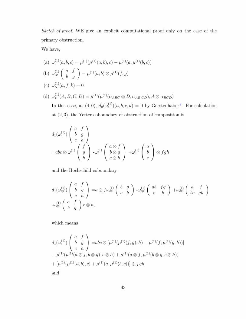
Sketch of proof. WE give an explicit computational proof only on the case of the

primary obstruction.

We have,

(a) ω(1)c (a, b, c) = µ(1)(µ(1)(a, b), c)− µ(1)(a, µ(1)(b, c))

(b) ω(1)cp

(a fb g

)= µ(1)(a, b)⊗ µ(1)(f, g)

(c) ω(1)N (a, f, k) = 0

(d) ω(1)P (A,B,C,D) = µ(1)(µ(1)(αABC ⊗D,αAB.CD), A⊗ αBCD)

In this case, at (4, 0), d0(ω(1)c )(a, b, c, d) = 0 by Gerstenhaber2. For calculation

at (2, 3), the Yetter coboundary of obstruction of composition is

d1(ω(1)c )

a fb gc h

=abc⊗ ω(1)

c

fgh

-ω(1)c

a⊗ fb⊗ gc⊗ h

+ω(1)c

abc

⊗ fghand the Hochschild coboundary

d1(ω(1)cp )

a fb gc h

=a⊗ fω(1)cp

(b gc h

)-ω

(1)cp

(ab fgc h

)+ω

(1)cp

(a fbc gh

)-ω

(1)cp

(a fb g

)c⊗ h,

which means

d1(ω(1)c )

a fb gc h

=abc⊗ [µ(1)(µ(1)(f, g), h)− µ(1)(f, µ(1)(g, h))]

− µ(1)(µ(1)(a⊗ f, b⊗ g), c⊗ h) + µ(1)(a⊗ f, µ(1)(b⊗ g, c⊗ h))

+ [µ(1)(µ(1)(a, b), c) + µ(1)(a, µ(1)(b, c))]⊗ fgh

and

43

d0(ω(1)cp )

a fb gc h

=a⊗ fµ(1)(b, c)⊗ µ(1)(f, g)− µ(1)(ab, c)⊗ µ(1)(fg, h)

+ µ(1)(a, bc)⊗ µ(1)(f, gh)− µ(1)(a, b)⊗ µ(1)(f, g)c⊗ h.

Since, the first order condition is that, µ(1) is a Hochschild cocycle, the com-

patibility condition gives

µ(1)(a⊗ f, b⊗ g) = µ(1)(a, b)⊗ fg + ab⊗ µ(1)(f, g),

d0(ω(1)cp )=abc⊗ [µ(1)(µ(1)(f, g), h)− µ(1)(f, µ(1)(g, h))]

− µ(1)(µ(1)(a, b)⊗ fg + ab⊗ µ(1)(f, g), c⊗ h)

+ µ(1)(a⊗ f, µ(1)(b, c)⊗ gh+ bc⊗ µ(1)(g, h))

+ [µ(1)(µ(1)(a, b), c) + µ(1)(a, µ(1)(b, c))]⊗ fgh

=abc⊗ µ(1)(µ(1)(f, g), h)− abc⊗ µ(1)(f, µ(1)(g, h))

− µ(1)(µ(1)(a, b), c)⊗ fgh− µ(1)(a, b)c⊗ µ(1)(fg, h)

− µ(1)(ab, c)⊗ µ(1)(f, g)h− abc⊗ µ(1)(µ(1)(f, g), h)

+ µ(1)(a, µ(1)(b, c))⊗ fgh+ aµ(1)(b, c)⊗ µ(1)(f, gh)

+ µ(1)(a, bc)⊗ fµ(1)(g, h) + abc⊗ µ(1)(f, µ(1)(g, h))

+ µ(1)(µ(1)(a, b), c)⊗ fgh+ µ(1)(a, µ(1)(b, c))⊗ fgh.

So,

d0(ω(1)cp ) + d1(ωc)

= −µ(1)(ab, c)⊗ µ(1)(f, g)h− µ(1)((a, b)c⊗ µ(1)(fg, h)

+ µ(1)(a, bc)⊗ fµ(1)(g, h) + aµ(1)(b, c)⊗ µ(1)(f, gh)

44

+ aµ(1)(b, c)⊗ fµ(1)(g, h)− µ(1)(ab, c)⊗ µ(1)(fg, h)

+ µ(1)(a, bc)⊗ µ(1)(f, gh)− µ(1)(a, b)c⊗ µ(1)(f, g)h


− µ(1)(ab, c)⊗ µ(1)(fg, h)− µ(1)(a, b)c⊗ µ(1)(f, g)h

+ µ(1)(a, bc)⊗ [fµ(1)(g, h) + µ(1)(f, gh)]

+ aµ(1)(b, c)⊗ [µ(1)(f, gh) + fµ(1)(g, h)]


− µ(1)(ab, c)⊗ µ(1)(fg, h)− µ(1)(a, b)c⊗ µ(1)(f, g)h

+ µ(1)(a, bc)⊗ [µ(1)(fg, h) + µ(1)(f, g)h]

+ aµ(1)(b, c)⊗ [µ(1)(f, g)h+ µ(1)(fg, h)]

= [aµ(1)(b, c)− µ(1)(ab, c) + µ(1)(a, bc)− µ(1)((a, b)c]

⊗ [µ(1)(f, g)h+ µ(1)(fg, h)] = 0.

At (3, 2), the coboundaries of the obstructions are

d1(ω(1)cp )

(a f kb g l

)= ab⊗ ω(1)

cp

(f kg l

)− ω(1)

cp

(a⊗ f kb⊗ g l

)+ ω

(1)cp

(a f ⊗ kb g ⊗ l

)− ω(1)

cp

(a fb g

)⊗ kl

=ab⊗ µ(1)(f, g)⊗ µ(1)(k, l)− µ(1)(a⊗ f, b⊗ g)µ(1)(k, l)

+ µ(1)(a, b)⊗ µ(1)(f ⊗ k, g ⊗ l)− µ(1)(a, b)⊗ µ(1)(f, g)⊗ kl

+ µ(1)(a, b)⊗ fg ⊗ µ(1)(k, l) = 0

Since ω(1)N (a, f, k) = 0; ω

(1)P (A,B,C,D) = 0, in the strict case by the iden-

tity preserving lemmas, we have,

45

d2(ωcp)(a f k m

)=ω

(1)cp

(αABC 1Da⊗ f.k m

)+ω

(1)cp

(1A αBCDa f ⊗ k.m

)-ω

(1)cp

(a f ⊗ k.m

1X αY ZW

)-ω

(1)cp

(a f ⊗ k.m

αXY Z 1W

)=0

d3(ω(1)cp )(A,B,C,D) = ω

(1)cp

(αABC ⊗D EαAB.CD E

)− ω(1)

cp

(αAB.CD EA⊗ αBCD E

)+ ω

(1)cp

(A αBCD ⊗ EA αBC.DE

)+ ω

(1)cp

(A αBC.DEA B ⊗ αCDE

)= 0

and similarly d4(ω(1)c ) = 0 = d3(ω

(1)c ). Hence, in this case, the obstructions

are cocycles.

2. Deforming tensor only

Theorem 2.1.2. All obstructions are cocycles when only tensor is deformed.

Sketch of proof. Again we give a computational proof only in the case of the primary

obstruction. We have,

a⊗f = a⊗ f + τ (1)(a, f)ε.

Then

(a) d0(τ (1)) (a fb g)

= a⊗ fτ (1)(f, k)− τ (1)(ab, fg)

46

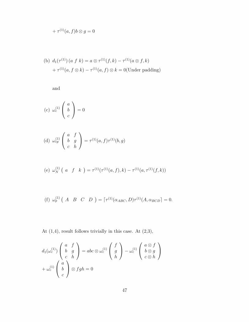
+ τ (1)(a, f)b⊗ g = 0

(b) d1(τ (1)) (a f k) = a⊗ τ (1)(f, k)− τ (1)(a⊗ f, k)

+ τ (1)(a, f ⊗ k)− τ (1)(a, f)⊗ k = 0(Under padding)

and

(c) ω(1)c

abc

= 0

(d) ω(1)cp

a fb gc h

= τ (1)(a, f)τ (1)(b, g)

(e) ω(1)N

(a f k

)= τ (1)(τ (1)(a, f), k)− τ (1)(a, τ (1)(f, k))

(f) ω(1)p

(A B C D

)= dτ (1)(αABC , D)τ (1)(A,αBCDe = 0.

At (1,4), result follows trivially in this case. At (2,3),

d1(ω(1)c )

a fb gc h

= abc⊗ ω(1)c

fgh

− ω(1)c

a⊗ fb⊗ gc⊗ h

+ ω

(1)c

abc

⊗ fgh = 0

47

d0(ω(1)cp )

a fb gc h

= a⊗ fω(1)cp

(b gc h

)− ω(1)

cp

(ab fgc h

)+ ω

(1)cp

(a fbc gh

)⊗ fgh− ω(1)

cp

(a fb g

)c⊗ h

= a⊗ fτ (1)(b, g)τ (1)(c, h)− τ (1)(ab, fg)τ (1)(c, h)

+ τ (1)(a, f)τ (1)(bc, gh)− τ (1)(a, f)τ (1)(b, g)c⊗ h

= [a⊗ fτ (1)(b, g)− τ (1)(ab, fg)]τ (1)(c, h)

+ τ (1)(a, f)[τ (1)(bc, gh)− τ (1)(b, g)c⊗ h]

= −τ (1)(a, f)b⊗ gτ (1)(c, h) + τ (1)(a, f)b⊗ gτ (1)(c, h) = 0

At(3,2),

d2(ω(1)c )

(a f kb g l

)= ω

(1)c

a.f ⊗ kb.g ⊗ lαXY Z

− ω(1)c

a.f ⊗ kαUVWb⊗ g.l

+ ω

(1)c

αABCa⊗ f.kb⊗ g.l

= 0

d0(ω(1)N )

(a f kb g l

)= [a b c ]Lω

(1)N

(a f k

)− ω(1)

N

(ab fg kl

)+ ω

(1)N

(a f k

)[f g h]R

= [a b c ]L[τ (1)(τ (1)(b, g), l)− τ (1)(b, τ (1)(g, l))]

+ τ (1)(ab, τ (1)(fg, kl)) + τ (1)(τ (1)(a, f), k)[f g h]R − τ (1)(a, τ (1)(f, k))[f g h]R

= [a b c ]Lτ(1)(τ (1)(b, g), l)− [a b c ]Lτ

(1)(b, τ (1)(g, l))

− τ (1)(τ (1)(a, f)b⊗ g, kl)− τ (1)(a⊗ fτ (1)(b, g), kl)

+ τ (1)(ab, τ (1)(f, k)g ⊗ l) + τ (1)(ab, f ⊗ kτ (1)(g, l))

+ τ (1)(τ (1)(a, f), k)[f g h]R − τ (1)(a, τ (1)(f, k))[f g h]R

= [a b c ]Lτ(1)(τ (1)(b, g), l)− [a b c ]Lτ

(1)(b, τ (1)(g, l))

− τ (1)(τ (1)(a, f), k)b.g ⊗ l − τ (1)(a, f)⊗ kτ (1)(b⊗ g, l)

48

− τ (1)(a⊗ f, k)τ (1)(b, g)⊗ l − a.f ⊗ kτ (1)(τ (1)(b, g), l)

+ a⊗ τ (1)(f, k)τ (1)(b, g ⊗ l) + τ (1)(a, τ (1)(f, k))b⊗ g.l

+ τ (1)(a, f ⊗ k)b⊗ τ (1)(g, l) + a⊗ f.kτ (1)(b, τ (1)(g, l))

+ τ (1)(τ (1)(a, f), k)[f g h]R − τ (1)(a, τ (1)(f, k))[f g h]R

= −τ (1)(a⊗ f, k)τ (1)(b, g)⊗ l + a⊗ τ (1)(f, k)τ (1)(b, g ⊗ l)

+ τ (1)(a, f ⊗ k)b⊗ τ (1)(g, l)− τ (1)(a, f)⊗ kτ (1)(b⊗ g, l)

d1(ω(1)cp )

(a f kb g l

)= ab⊗ ω(1)

cp

(f kg l

)− ω(1)

cp

(a⊗ f kb⊗ g l

)+ ω

(1)cp

(a f ⊗ kb g ⊗ l

)− ω(1)

cp

(a fb g

)⊗ kl

= ab⊗ τ (1)(f, k)τ (1)(g, l)− τ (1)(a⊗ f, k)τ (1)(b⊗ g, l)

+ τ (1)(a, f ⊗ k)τ (1)(b, g ⊗ l)− τ (1)(a, f)τ (1)(b, g)⊗ kl

= ab⊗ τ (1)(f, k)τ (1)(g, l)− [a⊗ τ (1)(f, k) + τ (1)(a, f ⊗ k)

− τ (1)(a.f)⊗ k][b⊗ τ (1)(g, l) + τ (1)(b, g ⊗ l)− τ (1)(b, g)⊗ l]

+ τ (1)(a, f ⊗ k)τ (1)(b, g ⊗ l)− τ (1)(a, f)τ (1)(b, g)⊗ kl

= −a⊗ τ (1)(f, k)τ (1)(b, g ⊗ l) + a⊗ τ (1)(f, k)τ (1)(b, g)⊗ l

− τ (1)(a, f)⊗ k)b⊗ τ (1)(g, l) + τ (1)(a, f ⊗ k)τ (1)(b, g)⊗ l

+ τ (1)(a, f)⊗ kb⊗ τ (1)(g, l) + τ (1)(a, f)⊗ kτ (1)(b, g ⊗ l)

− τ (1)(a, f)⊗ kτ (1)(b, g)⊗ l − τ (1)(a, f)⊗ kτ (1)(b, g)⊗ l

Thus combining, we get,

49

[d0(ω(1)N ) + d1(ω

(1)cp )]

(a f kb g l

)

= −a⊗ τ (1)(f, k)τ (1)(b, g ⊗ l) + a⊗ τ (1)(f, k)τ (1)(b, g)⊗ l

− τ (1)(a, f)⊗ k)b⊗ τ (1)(g, l) + τ (1)(a, f ⊗ k)τ (1)(b, g)⊗ l


− τ (1)(a, f)⊗ kτ (1)(b, g)⊗ l − τ (1)(a, f)⊗ kτ (1)(b, g)⊗ l

− τ (1)(a⊗ f, k)τ (1)(b, g)⊗ l + a⊗ τ (1)(f, k)τ (1)(b, g ⊗ l)

+ τ (1)(a, f ⊗ k)b⊗ τ (1)(g, l)− τ (1)(a, f)⊗ kτ (1)(b⊗ g, l)

= a⊗ τ (1)(f, k)τ (1)(b, g)⊗ l + τ (1)(a, f ⊗ k)τ (1)(b, g)⊗ l


− τ (1)(a, f)⊗ kτ (1)(b, g)⊗ l − τ (1)(a, f)τ (1)(b, g)⊗ kl

− τ (1)(a⊗ f, k)τ (1)(b, g)⊗ l − τ (1)(a, f)⊗ kτ (1)(b⊗ g, l)

= a⊗ τ (1)(f, k)τ (1)(b, g)⊗ l + τ (1)(a, f ⊗ k)τ (1)(b, g)⊗ l


− a⊗ τ (1)(f, k)τ (1)(b, g)⊗ l − τ (1)(a, f ⊗ k)τ (1)(b, g)⊗ l

− τ (1)(a, f)⊗ kτ (1)(b, g ⊗ l)− τ (1)(a, f)⊗ kb⊗ τ (1)(g, l) = 0

At (4,1),

d0(ω(1)P )(a f k m) = 0

d1(ω(1)N )(a f k m)

= a⊗ ω(1)N (f k m)− ω(1)

N (a⊗ f k m)

+ ω(1)N (a f ⊗ k m)− ω(1)

N (a f k ⊗m)

+ ω(1)N (a f k)⊗m

50

= a⊗ τ (1)(τ (1)(f, k),m)− a⊗ τ (1)(f, τ (1)(k,m))

− τ (1)(τ (1)(a⊗ f, k),m) + τ (1)(a⊗ f, τ (1)(k,m))

+ τ (1)(τ (1)(a, f ⊗ k),m)− τ (1)(a, τ (1)(f ⊗ k,m))

− τ (1)(τ (1)(a, f), k ⊗m) + τ (1)(a, τ (1)(f, k ⊗m))

+ τ (1)(τ (1)(a.f)k)⊗m− τ (1)(a, τ (1)(f, k))⊗m

= τ (1)(a⊗ τ (1)(f, k),m)− τ (1)(a, τ (1)(f, k)⊗m)

+ τ (1)(a, τ (1)(f, k)⊗m− τ (1)(a⊗ f, τ (1)(k,m)

+ τ (1)(a, f ⊗ τ (1)(k,m))− τ (1)(a, f)⊗ τ (1)(k,m)

− τ (1)(τ (1)(a⊗ f, k),m) + τ (1)(a⊗ f, τ (1)(k,m))

+ τ (1)(τ (1)(a, f ⊗ k),m)− τ (1)(a, τ (1)(f ⊗ k,m))

− τ (1)(τ (1)(a, f)k ⊗m) + τ (1)(a, τ (1)(f, k ⊗m))

+ τ (1)(a, f)⊗ τ (1)(k,m)− τ (1)(τ (1)(a, f)⊗ k,m)

+ τ (1)(τ (1)(a, f), k ⊗m)− τ (1)(a, τ (1)(f, k))⊗m

= τ (1)(a⊗ τ (1)(f, k),m)− τ (1)(τ (1)(a⊗ f, k),m)

+ τ (1)(τ (1)(a, f ⊗ k),m)− τ (1)(τ (1)(a, f)⊗ k,m)

+ τ (1)(a, f ⊗ τ (1)(k,m) + τ (1)(a, τ (1)(f ⊗ k,m))

+ τ (1)(a, τ (1)(f, k ⊗m))− τ (1)(a, τ (1)(f, k)⊗m)

− τ (1)(a⊗ f, τ (1)(k,m) + τ (1)(a⊗ f, τ (1)(k,m)

− τ (1)(τ (1)(a, f), k ⊗m) + τ (1)(τ (1)(a, f), k ⊗m)

= 0,

d2(ω(1)cp )(a f k m) = ω

(1)cp

(a.f ⊗ k mαXY Z 1W

)+ ω

(1)cp

a f.k ⊗m1X αY ZW

51

− ω(1)cp

(αABC 1Da⊗ f.k m

)− ω(1)

cp

(1A αBCDa f ⊗ k.m

)

= 0,

d3(ω(1)c )(a f k m) = ω

(1)c

((a.f).k).mαXY Z ⊗ 1WαXY.ZW

− ω(1)c

αABC ⊗ 1D(a.(f.k)).mαXY.ZW

+ ω

(1)cp

αABC ⊗ 1DαAB.CD

a.(f.(k.m))

+ ω(1)c

(a.(f.k)).mαXY.ZW

1X ⊗ αY ZW

− ω(1)c

αAB.CDa.((f.k).m)1X ⊗ αY ZW

+ ω

(1)c

αAB.CD1A ⊗ αBCDa.(f.(k.m))

− ω(1)c

((a.f).k).mαX.Y ZWαXY Z.W

+ ω(1)c

αA.BCD(a.f).(k.m)αXY Z.W

− ω(1)

c

αA.BCDαABC.D

a.(f.(k.m))

= 0,

and similarly, at (5,0), the coboundary of obstruction vanishes because inputs are

associators and objects only. So the result.

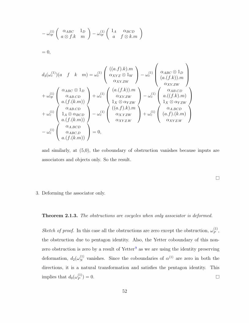
3. Deforming the associator only.

Theorem 2.1.3. The obstructions are cocycles when only associator is deformed.

Sketch of proof. In this case all the obstructions are zero except the obstruction, ω(1)P ,

the obstruction due to pentagon identity. Also, the Yetter coboundary of this non-

zero obstruction is zero by a result of Yetter9 as we are using the identity preserving

deformation, d2(ω(1)N vanishes. Since the coboundaries of α(1) are zero in both the

directions, it is a natural transformation and satisfies the pentagon identity. This

implies that d0(ω(1)P ) = 0.

52

2.1.2 Deforming two Structures at a Time

Theorem 2.1.4. All primary obstructions are cocycles when one of composition, tensor and

associator is undeformed.

Proof. 1. Tensor and the associator only are deformed (i.e. τ (1), α(1) 6= 0 and µ(1) = 0)

Then the first order conditions are:

(a) µ(1) = 0⇒ ω(1)c = 0.

(b) d0(τ (1))

(a fb g

)= τ (1)(a, f)b⊗ g − τ (1)(ab, fg)

+ a⊗ fτ (1)(b, g) = 0.

(c) d1(τ (1))(a f k

)= αABCa⊗ τ (1)(f, k)− τ (1)(a⊗ f, k)αXY Z

+ αABCτ(1)(a, f ⊗ k)− τ (1)(a, f)⊗ kαXY Z

= da⊗ τ (1)(f, k)e − dτ (1)(a⊗ f, k)e+ dτ (1)(a, f ⊗ k)

− dτ (1)(a, f)⊗ ke

= −d0(α(1))(a f k

)= −α(1)

ABCa⊗ f.k + a.f ⊗ kα(1)XY Z

(d) d2(τ (1))(A B C D

)= 0

(e) d1(α(1))(A B C D

)= dα(1)

ABC ⊗De − dα(1)A.BCDe

+ dα(1)AB.CDe − dα

(1)ABC.De+ dA⊗ α(1)

BCDeY etter

=∑4

i=0(−1)i∂iα(1) = 0

and the obstructions are:

(a) ω(1)cp

(a fb g

)= τ (1)(a, f)τ (1)(b, g)

53

(b) ω(1)N

(a f k

)= α

(1)ABCτ

(1)(a, f ⊗ k) + α(1)ABCa⊗ τ (1)(f, k)

+ αABCτ(1)(a, τ (1)(f, k))− τ (1)(τ (1)(a, f), k)αXY Z

− τ (1)(a⊗ f, k)α(1)XY Z − τ (1)(a, f)⊗ kα(1)

XY Z

(c) ω(1)P

(a f k

)= d[α(1)

ABC ⊗D]α(1)AB.CDe

+ d[α(1)ABC ⊗D][A⊗ α(1)

BCD]e+ dα(1)AB.CDA⊗ α

(1)BCDe

+ dτ (1)(α(1)ABC , D)e+ dτ (1)(A,α

(1)BCD)e − α(1)

A.BCDα(1)ABC.D.

Then we can easily see that, at (2,3)

d0(ω(1)cp )

a fb gc h

= 0 = d1(ω(1)c )

a fb gc h

.

At (3,2), we have,

d1(ω(1)cp )

(a f kb g l

)= ab⊗ ω(1)

cp

(f kg l

)− ω(1)

cp

(a⊗ f kb⊗ g l

)+ ω

(1)cp

(a f ⊗ kb g ⊗ l

)− ω(1)

cp

(a f ⊗ kb g

)⊗ kl

= αABCab⊗ τ (1)(f, k)τ (1)(g, l)− τ (1)(a⊗ f, k)τ (1)(b⊗ g, l)αXY Z

+ αABCτ(1)(a, f ⊗ k)τ (1)(b, g ⊗ l)− τ (1)(a, f)τ (1)(b, g)⊗ klαXY Z

= dab⊗ τ (1)(f, k)τ (1)(g, l)e − dτ (1)(a⊗ f, k)τ (1)(b⊗ g, l)e

+ dτ (1)(a, f ⊗ k)τ (1)(b, g ⊗ l)e − dτ (1)(a, f)τ (1)(b, g)⊗ kle

d0(ω(1)N )

(a f kb g l

)= a.f ⊗ kω(1)

N

(b g l

)− ω(1)

N

(ab fg kl

)+ ω

(1)N

(a f k

)b⊗ g.l

= a.f ⊗ k[α(1)UVW τ

(1)(b, g ⊗ l) + α(1)UVW b⊗ τ (1)(g, l)

+ αUVW τ(1)(b, τ (1)(g, l)− τ (1)(τ (1)(b, g), l)αXY Z

− τ (1)(b⊗ g, l)α(1)XY Z − τ (1)(b, g)⊗ lα(1)

XY Z ]

− [α(1)ABCτ

(1)(ab, fg ⊗ kl) + α(1)ABCab⊗ τ (1)(fg, kl)

54

+ αABCτ(1)(ab, τ (1)(fg, kl)− τ (1)(τ (1)(ab, fg), kl)αXY Z

− τ (1)(ab⊗ fg, kl)α(1)XY Z − τ (1)(ab, fg)⊗ klα(1)

XY Z ]

+ [α(1)ABCτ

(1)(a, f ⊗ k) + α(1)ABCa⊗ τ (1)(f, k)

+ αABCτ(1)(a, τ (1)(f, k)− τ (1)(τ (1)(a, f), k)αUVW

− τ (1)(a⊗ f, k)α(1)UVW − τ (1)(a, f)⊗ kα(1)

UVW ]b⊗ g.l.

Then,

[d0(ω(1)N )− d1(ω

(1)cp )]

(a f kb g l

)= a.f ⊗ k[α

(1)UVW τ

(1)(b, g ⊗ l) + α(1)UVW b⊗ τ (1)(g, l)

+ αUVW τ(1)(b, τ (1)(g, l)− τ (1)(τ (1)(b, g), l)αXY Z

− τ (1)(b⊗ g, l)α(1)XY Z − τ (1)(b, g)⊗ lα(1)

XY Z ]

− [α(1)ABCτ

(1)(ab, fg ⊗ kl) + α(1)ABCab⊗ τ (1)(fg, kl)

+ αABCτ(1)(ab, τ (1)(fg, kl)− τ (1)(τ (1)(ab, fg), kl)αXY Z

− τ (1)(ab⊗ fg, kl)α(1)XY Z − τ (1)(ab, fg)⊗ klα(1)

XY Z ]

+ [α(1)ABCτ

(1)(a, f ⊗ k) + α(1)ABCa⊗ τ (1)(f, k)

+ αABCτ(1)(a, τ (1)(f, k)− τ (1)(τ (1)(a, f), k)αUVW

− τ (1)(a⊗ f, k)α(1)UVW − τ (1)(a, f)⊗ kα(1)

UVW ]b⊗ g.l

− [dab⊗ τ (1)(f, k)τ (1)(g, l)e − dτ (1)(a⊗ f, k)τ (1)(b⊗ g, l)e

+ dτ (1)(a, f ⊗ k)τ (1)(b, g ⊗ l)e − dτ (1)(a, f)τ (1)(b, g)⊗ kle]

= [a.f ⊗ lα(1)UVW − α

(1)ABCa⊗ f.k][τ (1)(b, g ⊗ l) + b⊗ τ (1)(g, l)]

+ a.f ⊗ lαUVW τ (1)(b, τ (1)(g, l))− a.f ⊗ lτ (1)(b, τ (1)(g, l))αXY Z

− a.f ⊗ lτ (1)(b, g)⊗ lα(1)XY Z − a.f ⊗ lτ (1)(b⊗ g, l)α(1)

XY Z

− α(1)ABCτ

(1)(a, f ⊗ k)b⊗ g.l − α(1)ABCa⊗ τ (1)(f, k)b⊗ g.l

− αABCτ (1)(a, τ (1)(f, k)b⊗ g.l − αABCa⊗ τ (1)(f, k)τ (1)(b, g ⊗ l)

− αABCa⊗ f.kτ (1)(b, τ (1)(g, l))− αABCτ (1)(a, f ⊗ k)b⊗ τ (1)(g, l)

+ τ (1)(τ (1)(a, f), k)b.g ⊗ lαXY Z + τ (1)(a⊗ f, k)τ (1)(b, g)⊗ lαXY Z

55

+ a.f ⊗ kτ (1)(τ (1)(b, g), l)αXY Z + τ (1)(a, f)⊗ kτ (1)(b⊗ g, l)αXY Z

+ [τ (1)(a, f)⊗ k + τ (1)(a⊗ f, k)][b.g ⊗ lα(1)XY Z − α

(1)UVW b⊗ g.l]

+ a.f ⊗ kτ (1)(b, g)⊗ lα(1)XY Z + a.f ⊗ kτ (1)(b⊗ g, l)α(1)

XY Z

+ α(1)ABCτ

(1)(a, f ⊗ k)b⊗ g.l + α(1)ABCa⊗ τ (1)(f, k)b⊗ g.l

+ αABCτ(1)(a, τ (1)(f, k))b⊗ g.l − τ (1)(τ (1)(a, f), k)αUVW b⊗ g.l

− [αABCab⊗ τ (1)(f, k)τ (1)(g, l)− τ (1)(a⊗ f, k)τ (1)(b⊗ g, l)αXY Z

+ αABCτ(1)(a, f ⊗ k)τ (1)(b, g ⊗ l)− τ (1)(a, f)τ (1)(b, g)⊗ klαXY Z ].

Now using the first order conditions, the above expression,

= [αABCa⊗ τ (1)(f, k)− τ (1)(a⊗ f, k)αUVW + αABCτ(1)(a, f ⊗ k)

− τ (1)(a, f)⊗ kαUVW ][τ (1)(b, g ⊗ l) + b⊗ τ (1)(g, l)]

+ a.f ⊗ lαUVW τ (1)(b, τ (1)(g, l))− a.f ⊗ lτ (1)(b, τ (1)(g, l))αXY Z

− a.f ⊗ lτ (1)(b, g)⊗ lα(1)XY Z − a.f ⊗ lτ (1)(b⊗ g, l)α(1)

XY Z

− α(1)ABCτ

(1)(a, f ⊗ k)b⊗ g.l − α(1)ABCa⊗ τ (1)(f, k)b⊗ g.l

− αABCτ (1)(a, τ (1)(f, k)b⊗ g.l − αABCa⊗ τ (1)(f, k)τ (1)(b, g ⊗ l)

− αABCa⊗ f.kτ (1)(b, τ (1)(g, l))− αABCτ (1)(a, f ⊗ k)b⊗ τ (1)(g, l)

+ τ (1)(τ (1)(a, f), k)b.g ⊗ lαXY Z + τ (1)(a⊗ f, k)τ (1)(b, g)⊗ lαXY Z

+ a.f ⊗ kτ (1)(τ (1)(b, g), l)αXY Z + τ (1)(a, f)⊗ kτ (1)(b⊗ g, l)αXY Z

+ [τ (1)(a, f)⊗ k + τ (1)(a⊗ f, k)][αUVW b⊗ τ (1)(g, l)

− τ (1)(b⊗ g, l)αXY Z + αUVW τ(1)(b, g ⊗ l)− τ (1)(b, g)⊗ lαXY Z ]

+ a.f ⊗ kτ (1)(b, g)⊗ lα(1)XY Z + a.f ⊗ kτ (1)(b⊗ g, l)α(1)

XY Z

+ α(1)ABCτ

(1)(a, f ⊗ k)b⊗ g.l + α(1)ABCa⊗ τ (1)(f, k)b⊗ g.l


− [αABCab⊗ τ (1)(f, k)τ (1)(g, l)− τ (1)(a⊗ f, k)τ (1)(b⊗ g, l)αXY Z

+ αABCτ(1)(a, f ⊗ k)τ (1)(b, g ⊗ l)

− τ (1)(a, f)τ (1)(b, g)⊗ klαXY Z ] = 0.

56

At (4,1), proof is in Appendix A.

At (5,0), all the coboundaries of obstructions are zero except for d1(ω(1)P ). Now

d1(ω(1)P )(A,B,C,D,E) = A⊗ω(1)

P (B,C,D,E)−ω(1)P (A.B,C,D,E)+ω

(1)P (A,B.C,D,E)

− ω(1)P (A,B,C.D,E) + ω

(1)P (A,B,C,D.E)− ω(1)

P (A,B,C,D)⊗ E

= A⊗ [α(1)BCD ⊗ 1Eα

(1)BC.DE + α

(1)BCD ⊗ 1E1B ⊗ α(1)

CDE + α(1)BC.DE1B ⊗ α(1)

CDE

− α(1)B.CDEα

(1)BCD.E + τ (1)(α

(1)BCD, 1E) + τ (1)(1B, α

(1)CDE)]

− [α(1)A.BCD ⊗ 1Eα

(1)A.BC.DE + α

(1)A.BCD ⊗ 1E1A.B ⊗ α(1)

CDE + α(1)A.BC.DE1A.B ⊗ α(1)

CDE

− α(1)(A.B).CDEα

(1)A.BCD.E + τ (1)(α

(1)A.BCD, 1E) + τ (1)(1A.B, α

(1)CDE)]

+ [α(1)AB.CD ⊗ 1Eα

(1)A(B.C).DE + α

(1)AB.CD ⊗ 1E1A ⊗ α(1)

B.CDE + α(1)A(B.C).DE1A ⊗ α(1)

B.CDE

− α(1)A(B.C).DEα

(1)AB.CD.E + τ (1)(α

(1)AB.CD, 1E) + τ (1)(1A, α

(1)B.CDE)]

− [α(1)ABC.D ⊗ 1Eα

(1)AB(C.D).E + α

(1)ABC.D ⊗ 1E1A ⊗ α(1)

BC.DE + α(1)AB(C.D).E1A ⊗ α(1)

BC.DE

− α(1)AB(C.D).Eα

(1)AB(C.D).E + τ (1)(α

(1)ABC.D, 1E) + τ (1)(1A, α

(1)BC.DE)]

+ [α(1)ABC ⊗ 1D.Eα

(1)ABC.(D.E) + α

(1)ABC ⊗ 1D.E1A ⊗ α(1)

BCD.E + α(1)ABC.(D.E)1A ⊗ α

(1)BCD.E

− α(1)ABC.(D.E)α

(1)ABC.(D.E) + τ (1)(α

(1)ABC , 1D.E) + τ (1)(1A, α

(1)BCD.E)]

− [α(1)ABC ⊗ 1Dα

(1)ABC.D + α

(1)ABC ⊗ 1D1A ⊗ α(1)

BCD + α(1)ABC.D1A ⊗ α(1)

BCD

− α(1)ABC.Dα

(1)ABC.D + τ (1)(α

(1)ABC , 1D) + τ (1)(1A, α

(1)BCD)]⊗ E.

In this case, since the first order condition on the pentagon is exactly the first or-

der condition of Yetter’s case as we are assuming the identity preserving case, all the

terms except those containing τ (1) vanish by Yetter9. Using the pentagon identity

inside the arguments of τ (1) and then the first order condition from preservation of

identity (lemma 2.0.4), we can see that the other terms also vanish.

2. Composition and tensor are deformed (i.e. µ(1), τ (1) 6= 0 and α(1) = 0).

The first order conditions are

57

(a) d0(µ(1))

abc

= aµ(1)(b, c)− µ(1)(ab, c) + µ(1)(a, bc)− µ(1)(a, b)c = 0.

(b) d1(µ(1))

(a fb g

)= abµ(1)(f, g)− µ(1)(a⊗ f, b⊗ g) + µ(1)(a, b)⊗ fg.

(c) d2(µ(1))(a f k

)= µ(1)(αABC , a⊗ f.k)− µ(1)(a.f ⊗ k, αXY Z) = 0.

(d) d0(τ (1))

(a fb g

)= a⊗ fτ (1)(b, g)− τ (1)(ab, fg) + τ (1)(a, f)b⊗ g.

d0(τ (1)) = d1(µ(1))

(e) d1(τ (1))(a f k

)= αABCa⊗ τ (1)(f, k)− τ (1)(a.f, k)αXY Z + αABCτ

(1)(a, f.k)

−τ (1)(a, f)⊗ kαXY Z = 0 since α(1) = 0.

(f) d3(µ(1))(A B C D

)= µ(1)(αABC ⊗D,αAB.CD)

−µ(1)(αA.BCD, αABC.D) + µ(1)(αABC ⊗DαAB.CD, A⊗ αBCD) = 0

since α(1) = 0.

And obstructions,

(a) ω(1)c

abc

= µ(1)(µ(1)(a, b), c)− µ(1)(a, µ(1)(b, c))

(b) ω(1)cp

(a fb g

)= µ(1)(τ (1)(a, f), b⊗g)−µ(1)(a, b)⊗µ(1)(f, g)+µ(1)(a⊗f, τ (1)(b, g))

−τ (1)(µ(1)(a, b), fg) + τ (1)(a, f)τ (1)(b, g)− τ (1)(ab, µ(1)(f, g))

58

(c) ω(1)N

(a f k

)= αABCτ

(1)(τ (1)(a, f), k)− τ (1)(a, τ (1)(a, , k))αXY Z

(d) ω(1)P

(A B C D

)= 0

At (1,4), d0(ω(1)c )

abcd

= 0 by Gerstenhaber.

At (2,3), d1(ω(1)c )

a fb gc h

= abc⊗ ω(1)c

fgh

+ω

(1)c

a⊗ fb⊗ gc⊗ h

− ω(1)c

abc

⊗ fgh= abc⊗ µ(1)(µ(1)(f, g), h)− abc⊗ µ(1)(f, µ(1)(g, h))− µ(1)(µ(1)(a.f, b.), c.h)

+ µ(1)(a.f, µ(1)(b.g, c.h)) + µ(1)(µ(1)(a, b), c)⊗ fgh− µ(1)(a, µ(1)(b, c))⊗ fgh

d0(ω(1)cp )

a fb gc h

= a⊗(b gc h

)−(ab fgc h

)+

(a fbc gh

)−(a fb g

)c⊗ h

= a⊗ fµ(1)(τ (1)(b, g), c.h) + a⊗ fµ(1)(b.g, τ (1)(c, h)) + a⊗ fτ (1)(b, g)τ (1)(c, h)

− a⊗ fτ (1)(µ(1)(b, c), gh)− a⊗ fτ (1)(bc, µ(1)(g, h))− a⊗ fµ(1)(b, v)⊗ µ(1)(g, h)

− µ(1)(τ (1)(ab, fg), c.h)− µ(1)(ab.fg, τ (1)(c, h))− τ (1)(ab, fg)τ (1)(c, h)

+ τ (1)(µ(1)(ab, c), fgh) + τ (1)(abc, µ(1)(fg, h)) + µ(1)(ab, c)⊗ µ(1)(fg, h)

+ µ(1)(τ (1)(a, f)bc.gh) + µ(1)(a.f, τ (1)(bc, gh)) + τ (1)(a, f)τ (1)(bc, gh)

− τ (1)(µ(1)(a, bc), fgh)− τ (1)(abc, µ(1)(f, gh))− µ(1)(a, bc)⊗ µ(1)(f, gh)

− µ(1)(τ (1)(a, f), b.g)c.h− µ(1)(a.f, τ (1)(b, g))c.h− τ (1)(a, f)τ (1)(b, g)c.h

+ τ (1)(µ(1)(a, b), fg)c.h+ τ (1)(ab, µ(1)(f, g))c, h+ µ(1)(a, b)⊗ µ(1)(f, g)c.h

= a⊗ fµ(1)(τ (1)(b, g), c.h) + a⊗ fµ(1)(b.g, τ (1)(c, h)) + a⊗ fτ (1)(b, g)τ (1)(c, h)

59

− a⊗ fτ (1)(µ(1)(b, c), gh)− a⊗ fτ (1)(bc, µ(1)(g, h))− a⊗ fµ(1)(b, v)⊗ µ(1)(g, h)

− µ(1)(τ (1)(a, f)b.g, c.h)− µ(1)(µ(1)(a.f, b.g), c.h)− µ(1)(a.f, τ (1)(b, g), c.h)

+ µ(1)(µ(1)(a, b).fg, c.h) + µ(1)(ab.µ(1)(f, g), c.h)− µ(1)(ab.fg, τ (1)(c, h))

− τ (1)(a, f)b.gτ (1)(c, h)− µ(1)(a.f, b.g)τ (1)(c, h)− a.f, τ (1)(b, g)τ (1)(c, h)

+ µ(1)(a, b).fgτ (1)(c, h) + ab.µ(1)(f, g)τ (1)(c, h) + τ (1)(µ(1)(ab, c), fgh)

+ τ (1)(abc, µ(1)(fg, h)) + µ(1)(ab, c)⊗ µ(1)(fg, h) + µ(1)(τ (1)(a, f), bc.gh)

+ µ(1)(a.f, τ (1)(b, g)c.h) + µ(1)(a.f, µ(1)(b.g, c.h)) + µ(1)(a.f, b.gτ (1)(c, h))

− µ(1)(a.f, µ(1)(b, g)⊗ gh)− µ(1)(a.f, bc⊗ µ(1)(g, h)) + τ (1)(a, f)τ (1)(b, g)c.h

+ τ (1)(a, f)µ(1)(b.g, c.h) + τ (1)(a, f)b.gτ (1)(c, h) + τ (1)(a, f)µ(1)(b, g)⊗ gh

+ τ (1)(a, f)bc⊗ µ(1)(g, h)− τ (1)(µ(1)(a, bc), fgh)− τ (1)(abc, µ(1)(f, gh))

− µ(1)(a, bc)⊗ µ(1)(f, gh)− µ(1)(τ (1)(a, f), b.g)c.h− µ(1)(a.f, τ (1)(b, g))c.h

− τ (1)(a, f)τ (1)(b, g)c.h+ τ (1)(µ(1)(a, b), fg)c.h

+ τ (1)(ab, µ(1)(f, g))c, h+ µ(1)(a, b)⊗ µ(1)(f, g)c.h

1st order condition= a⊗fτ (1)(b, g)τ (1)(c, h)−a⊗fτ (1)(µ(1)(b, c), gh)−a⊗fτ (1)(bc, µ(1)(g, h))

− a⊗ fµ(1)(b, v)⊗ µ(1)(g, h)− µ(1)(µ(1)(a.f, b.g), c.h) + µ(1)(µ(1)(a, b).fg, c.h)

+ µ(1)(ab.µ(1)(f, g), c.h) + µ(1)(a, b).fgτ (1)(c, h) + ab.µ(1)(f, g)τ (1)(c, h)

+ τ (1)(µ(1)(ab, c), fgh) + τ (1)(abc, µ(1)(fg, h)) + µ(1)(ab, c)⊗ µ(1)(fg, h)

+ µ(1)(a.f, µ(1)(b.g, c.h))− µ(1)(a.f, µ(1)(b, g)⊗ gh)− µ(1)(a.f, bc⊗ µ(1)(g, h))

+ τ (1)(a, f)µ(1)(b, g)⊗ gh+ τ (1)(a, f)bc⊗ µ(1)(g, h)− τ (1)(µ(1)(a, bc), fgh)

− τ (1)(abc, µ(1)(f, gh))− µ(1)(a, bc)⊗ µ(1)(f, gh) + τ (1)(µ(1)(a, b), fg)c.h

+ τ (1)(ab, µ(1)(f, g))c, h+ µ(1)(a, b)⊗ µ(1)(f, g)c.h

Combining, we get

[d1(ω(1)c )− d0(ω

(1)cp )]

a fb gc h

= abc⊗ µ(1)(µ(1)(f, g), h)− abc⊗ µ(1)(f, µ(1)(g, h))

+ µ(1)(µ(1)(a, b), c)⊗ fgh− µ(1)(a, µ(1)(b, c)⊗ fgh

+ a.fτ (1)(b, c), gh) + a.fτ (1)(bc, µ(1)(g, h) + a.dµ(1)(b, c)⊗ µ(1)(g, h)

60

− µ(1)(µ(1)(a, b).fg, c.h)− µ(1)(ab.µ(1)(f, g), c.h)− µ(1)(a, b).fgτ (1)(c, h)

− ab.µ(1)(f, g)τ (1)(c, h)− τ (1)(µ(1)(ab, c), fgh)− τ (1)(abc, µ(1)(fg, h))

− µ(1)(ab, c).µ(1)(fg, h) + µ(1)(a.f, µ(1)(c, b.gh) + µ(1)(a.f, bc.µ(1)(g, h))

+ τ (1)(a, f)µ(1)(b, c).gh+ τ (1)(a.f)bc.µ(1)(g, g) + τ (1)(µ(1)(a, bc), fgh)

+ τ (1)(abc, µ(1)(f, gh)) + µ(1)(a, bc).µ(1)(f, gh)

− τ (1)(µ(1)(a, b), fg)c.h− τ (1)(ab, µ(1)(f, g)c.h− µ(1)(a, b).µ(1)(f, g)c⊗ h

Using the first condition on

(µ(1)(a, b) fg

c h

)and such hexagons, we find that the

difference is

= a.fµ(1)(b, c).µ(1)(g, h)− µ(1)(a, b).µ(1)(f, g)c⊗ h

− τ (1)(µ(1)(ab, c), fgh)− τ (1)(abc, µ(1)(fg, h)− µ(1)(ab, c).µ(1)(fg, h)

+ τ (1)(µ(1)(a, bc), fgh) + τ (1)(abc, µ(1)(f, gh)) + µ(1)(a, bc).µ(1)(f, gh)

− µ(1)(a, b)c.µ(1)(fg, h)− τ (1)(µ(1)(a, b)c, fgh)− µ(1)(ab, c).µ(1)(f, g)h

− τ (1)(abc, µ(1)(f, g)h) + µ(1)(a, bc).fµ(1)(g, h) + τ (1)(abc, fµ(1)(g, h))

+ aµ(1)(b, c).µ(1)(f, gh) + τ (1)(aµ(1)(b, c), fgh) + τ (1)(aµ(1)(b, c), fgh)

= aµ(1)(b, c).fµ(1)(g, h)− µ(1)(a, b)c.µ(1)(f, g)h− µ(1)(ab, c).µ(1)(fg, h)

+ µ(1)(a, bc).µ(1)(f, gh)− µ(1)(a, b)c.µ(1)(fg, h)− µ(1)(ab, c).µ(1)(f, g)h

+ µ(1)(a, bc).fµ(1)(g, h) + aµ(1)(b, c).µ(1)(f, gh)

= aµ(1)(b, c).fµ(1)(g, h) + µ(1)(a, bc).µ(1)(f, gh)

+ aµ(1)(b, c).µ(1)(f, gh) + µ(1)(a, bc).fµ(1)(g, h)

− µ(1)(a, b)c.[µ(1)(f, g)h+ µ(1)(fg, h)]− µ(1)(ab, c).[µ(1)(fg, h) + µ(1)(f, g)h]

= aµ(1)(b, c).fµ(1)(g, h) + µ(1)(a, bc).µ(1)(f, gh)

+ aµ(1)(b, c).µ(1)(f, gh) + µ(1)(a, bc).fµ(1)(g, h)

− µ(1)(a, b)c.[µ(1)(f, gh) + fµ(1)(g, h)]− µ(1)(ab, c).[fµ(1)(g, h) + µ(1)(f, gh)]

61

= d1(µ(1))(a, b, c)[fµ(1)(g, h) + µ(1)(f, gh)] = 0

At (3,2), this is a special case of the proof in Appendix A.

At (4,1), we have

ω(1)P = 0 and so d0(ω

(1)P ) = 0.

Also, d2(ω(1)cp ) = 0 = d3(ω

(1)c ). To prove the result, we need to see d1(ω

(1)N ) = 0. For

this,

d1(ω(1)N )(a f k m

)= a.ω

(1)N (f, k,m)− ω(1)

N (a.f, k,m)

+ ω(1)N (a, f.k,m)− ω(1)

N (a, f, k.m) + ω(1)N (a, f, k).m

= a.τ (1)(τ (1)(τ (1)(f, k),m)− a.τ (1)(f, τ (1)(k,m)− τ (1)(τ (1)(a.f, k),m)

+ τ (1)(a.f, τ (1)(k,m)) + τ (1)(τ (1)(a, f.k),m)− τ (1)(a, τ (1)(f.k,m))

− τ (1)(τ (1)(a, f), k.m) + τ (1)(a, τ (1)(f, k.m)) + τ (1)(τ (1)(a, f), k).m

+ τ (1)(a, τ (1)(f, k)).m

= τ (1)(a.τ (1)(f, k),m)− τ (1)(a, τ (1)(f, k).m) + τ (1)(a, τ (1)(f, k)).m

− τ (1)(a.f, τ (1)(k,m)) + τ (1)(a, f.τ (1)(k,m))− τ (1)(a, f).τ (1)(k,m)

− τ (1)(τ (1)(a.f, k),m) + τ (1)(a.f, τ (1)(k,m)) + τ (1)(τ (1)(a, f.k),m)

− τ (1)(a, τ (1)(f.k,m))− τ (1)(τ (1)(a, f), k.m) + τ (1)(a, τ (1)(f, k.m))

+ τ (1)(a, f).τ (1)(k,m)− τ (1)(τ (1)(a, f).k,m) + τ (1)(τ (1)(a, f), k.m)

+ τ (1)(a, τ (1)(f, k)).m = 0

At (5,0), all the coboundaries of all obstructions are 0s. Hence, the obstructions

are cocycles in this case too.

62

3. Composition and the associator only are deformed (i.e. µ(1), α(1) 6= 0 and τ (1) = 0).

The first order conditions are

(a) d0(µ(1))

abc

= aµ(1)(b, c)− µ(1)(ab, c) + µ(1)(a, bc)− µ(1)(a, b)c = 0.

(b) d1(µ(1))

(a fb g

)= abµ(1)(f, g)− µ(1)(a⊗ f, b⊗ g) + µ(1)(a, b)⊗ fg = 0.

(c) d2(µ(1))(a f k

)= µ(1)(αABC , a⊗ f.k)− µ(1)(a.f ⊗ k, αXY Z) = 0.

(d) d0(τ (1))

(a fb g

)= 0.

d0(τ (1)) = d1(µ(1)) = 0

(e) d1(τ (1))(a f k

)= 0.

(f) d3(µ(1))(A B C D

)= µ(1)(αABC ⊗D,αAB.CD)− µ(1)(αA.BCD, αABC.D)

+µ(1)(αABC ⊗DαAB.CD, A⊗ αBCD) = 0, since α(1) = 0.

And obstructions,

(a) ω(1)c

abc

= µ(1)(µ(1)(a, b), c)− µ(1)(a, µ(1)(b, c))

(b) ω(1)cp

(a fb g

)= µ(1)(a, b)⊗ µ(1)(f, g)

63

(c) ω(1)N

(a f k

)= µ(1)(α

(1)ABC , a⊗ f.k)− µ(1)(a.f ⊗ k, α(1)

XY Z)

(d) ω(1)P

(A B C D

)= α

(1)ABC ⊗Dα

(1)AB.CD + α

(1)ABC ⊗DA⊗ α

(1)BCD

+α(1)AB.CDA⊗ α

(1)BCD − α

(1)A.BCDα

(1)ABC.D

under Yetter’s padded composition.

As before, at (1,4) is Gerstenhaber’s proof, at (2,3) and (3,2) are the particular cases

of previous composition and tensor case and the appendix respectively. At (4,1)

d3(ω(1)c ) = 0 = d2(ω

(1)cp )

For the other differentials of obstruction, as α(1) is natural in this case, vanishes inde-

pendently.

At (5,0), all the coboundaries of obstructions are zero except the Yetter cobound-

ary of ω(1)P . Since, we are assuming the category is strict one, this is also cocycle by a

result of Yetter9.

Thus the result follows.

2.2 A Geometrical Approach to Simplify Messy Cal-

culations

We have seen that the direct calculation of the coboundaries of obstructions, even in spe-

cial cases are not simple. So, to handle the general case, we will use geometrical encoding

of the obstructions and cobounding conditions. For this we are going to construct poly-

tope or cell decomposition of sphere such that edges of each face represent the deformable

arrow-valued operations and with them the corresponding deformation terms of each or-

der and each face represents both relations the deformation terms satisfy up to some order

and instances of an obstruction entry of each order greater than one depending on how the

operations around a face are assembled, or a difference of terms which must trivially be zero.

64

As an example, consider the first order obstruction of deformation of composition is given by

ω(1)(a, b, c) = µ(1)(µ(1)(a, b), c)− µ(1)(a, µ(1)(b, c)),

and the first order condition is given by

aµ(1)(b, c)− µ(1)(ab, c) + µ(1)(a, bc)− µ(1)(a, b)c = 0.

Those two conditions can be represented by the following square:

a(bc)//

.ab

//

bc

OO

(ab)c.

OO

We can call it, square [a, b, c]. For the first order condition, we are taking one degree de-

formation from each edge and the orientation gives the sign of the terms on the expression.

But, we need to remember that each term should have all the arrows used. So, the first side

on the clockwise direction gives us the first term of the first order condition and the second

gives us the third term. Similarly, the other sides give us the second and last term of the

same.

For the first obstruction terms, we use the same sign rule, but spread a total degree of

two over the edges of each oriented “half” of the boundary so that each edge gets at most

one. Similarly, second order condition, we spread degree 2 in all possible ways keeping the

sign rule in mind, which gives

65

aµ(2)(b, c) + µ(2)(a, bc) + µ(1)(a, µ(1)(b, c)) = µ(2)(a, b) + µ(2)(ab, c) + µ(1)(µ(1)(a, b), c). Note

that this is equivalent to the condition that the Hochschild coboundary of µ(1) equals the

first obstruction ω(1). The second obstruction can be obtained as spreading the degree 3 in

all possible ways such that each edge gets at most degree 2. That is,

ω(2)c (a, b, c) = µ(2)(µ(1)(a, b), c) + µ(1)(µ(2)(a, b), c)− µ(2)(a, µ(1)(b, c))− µ(1)(a, µ(2)(b, c)).

In general, spreading total degree n over all edges on each of the two halves of the boundary,

so then each edge has degree less than n and taking the difference gives the obstruction to

extend to degree n, which letting the edges have degrees up to and including n gives the nth

order condition that µ(n) cobounds ω(n).

Now, the Gerstenhaber cocycle condition of obstruction to deformation of associative com-

position can be calculated from a polytope, whose edges represent deformable structures,

here the composition only,

.(abc)d

//

.

abc

BB cd // .

ab(cd)

AA

.

a(bc)

OO (bc)d

//_________________ .

a(bcd)

OO

ab

OO

bc

AA

cd // .

bcd

AA

ab

OO

66

To keep track of the calculations of the cocycle condition for the obstructions to deformation

of composition from chapter 1, the lowest face is the square [b, c, d], the top face is the

square [ab,c,d], the back face is the square [a,bc,d], the right face it the square [a,b,cd], the

left one is the square [a, b, c] and the front face is a trivial square.

In the calculations in the proofs of Proposition 1.2.3 and Theorem 1.2.4, we used instances

of the lower order conditions (that µ(1) is a coboundary and that each µ(k) cobounds the

kth obstruction) on each face to replace instances of the label on the common edge abc on

the other face with expressions not involving the common label, thereby showing that the

sum of the obstruction-type expressions on the square [ab, c, d] and the square [a, b, c] equals

the obstruction-like expression corresponding to the hexagon obtained by gluing the squares

on their common edge by spreading the total degree among the edges of each oriented side

as described above for the squares. Similarly, we glued the squares [b, c, d] and [a, b, cd]

through the common edge bcd. In the proof of Theorem 1.2.4 these steps occur where the

nested summations first appear. The remaining sides (the trivial front, and [a, bc, d]) glue

on even more trivially: the terms corresponding to one half of the boundary cancel some of

those in the hexagons obtained by the previous gluing, and the result is an obstruction like

expression corresponding to the hexagon with edges ab, cd, ab(cd), bc, (bc)d, and a(bcd),

occurring twice with opposite signs.

This suggests taking a geometrical approach to proving the obstructions are cocycles if

we can get suitable cell decomposition of a sphere, with edges labeled by instances of arrow-

valued operations for each of the bidegrees (1,2), (2,3), (3,2), (4,1) and (5,0).

Consider a polygon whose edges are labeled with instances of deformable arrow-valued

operations which are either arrow (or object) variables or values of arrow-valued operations

67

occurring earlier on a path from a global source to a global target. Each polygon encodes

a equational condition at each order: the vanishing of the difference of the expressions re-

sulting from spreading the order among the edges of the two directed paths in all possible

way with the sign chosen by which path is reveal to give the boundary orientation. Each

polygon encodes an obstruction-type expression at each order greater or equal to one: such

that the difference of the expressions in which the total order could all be on a single edge

(with other order 0).

Definition 2.2.1. (Admissible and Non-admissible Polygon Combinations) Two polygons

with edges representing arrow-valued operations with one source and one target are called

admissible if when they are glued together on the edges which represent same instance of an

arrow-valued operation, the boundary of resulting polygon has unique source and target.

Example:

//___ • //__ • //___ • //___ •FF

XX22

22

2

FF

XX00

00

0

FF

XX00

00

0

FF

XX00

00

0OO

OO

//////////

OO OO OO OO

WW////////////

FF //

GG

WW////////////

GG //

WW//////////

GG

These combination of polygons are non-admissible because they have not unique source and

targets for the boundary polygon. So, we see that if the sharing side(s) is(are) dissolved,

the polygon will not have unique either source or target in this case. But the polygons,

68

//

1

11

11

1 //___ • • //___ •FF •

FF

XX11

11

11

FF

YY22

22

22

XX11

11

11

OO

OO

111111111111

OO OO OO OO

XX111111111111//

FF //

FF

XX111111111111

EE

FF oo_ _ _

are admissible because they have unique source and target if the shared side(s) is(are) dis-

solved.

Lemma 2.2.1. If two polygons have sides representing arrow-valued deformable structures,

the first order conditions described by both polygons hold and they are admissible, then the

sum of the second order obstruction-type expressions given by the two polygons is equal to

the obstruction-type expression given by the larger polygon obtained by deleting the shared

edges.

Proof. Consider two polygons each with one source and one target and are admissible. The

sides of this polygon are represented as:

69

//

fa

3

33

33

33

3kd //____ •

...

EE •

k2

EE

gc

YY33

33

33

33

f2

OO

gb k1

OO

h1

333333333333333

...

OO

f1

YY333333333333333

g1//

g2

EEh2

//

h3

EE

.

One side of the first polygon is denoted by arrows f ′is, i = 1, 2, ..., a and on the other side is

denoted by arrows g′is, i = 1, 2, ..., b. Similarly, for the other polygon,h′is, i = 1, 2, ..., c and

k′is, i = 1, 2, ..., d respectively.

If we are considering only first order deformation of arrows, i.e.

fi = fi + f(1)i ε and gj = gj + g

(1)j ε where i = 1, 2, ..., a and i = 1, 2, ..., b. Then the first order

condition is given by, ∑1≤i≤a

f(1)i −

∑1≤j≤b

g(1)j = 0.

The first obstruction of deformation on the boundary is given by,

∑1≤i<j≤a

f(1)i f

(1)j −

∑1≤p<q≤b

g(1)p g(1)

q .

Now, gluing a polygonal face which satisfy the admissible condition in our sense. Assume

that the side common to both polygons is gb and the arrows on the g-side are given by

hp’s, p = 1, 2, ..., c, and that on the f -side are given by kq, q = 1, 2, ..., d, i.e. gb = k1 and

hp = hp + h(1)p ε and kp = kp + k

(1)p ε where p = 1, 2, ..., c and q = 1, 2, ..., d. Then the first

order condition on the second polygon is

70

∑1≤r≤c

h(1)r −

∑1≤s≤d

k(1)s = 0,

and the first obstruction is

∑1≤r<s≤c

h(1)r h(1)

s −∑

1≤t<u≤d

k(1)t k(1)

u .

Then, for the resulting polygon, we want to get the result from the condition from the

individual polygon as;

Note that k1 = gb. So, then solving the value of k1 from the first order condition of second

polygon and substituting it to the first order condition from the first polygon, that is,

g(1)b = k1 =

∑1≤r≤c

h(1)r −

∑1<s≤d

k(1)s ,

and so,

0 =∑

1≤i≤a

f(1)i −

∑1≤j≤b

g(1)j =

∑1≤i≤a

f(1)i −

∑1≤j<b

g(1)j − g

(1)b

=∑

1≤i≤a

f(1)i −

∑1≤j<b

g(1)j − [

∑1≤r≤c

h(1)r −

∑1<s≤d

k(1)s ]

= [∑

1≤i≤a

f(1)i +

∑1<s≤d

k(1)s ]− [

∑1≤r≤c

h(1)r +

∑1<s≤d

k(1)s ].

which is the first order condition on the boundary of glued polygon. Also,

∑1≤i<j≤a

f(1)i f

(1)j −

∑1≤p<q≤b

g(1)p g(1)

q =∑

1≤i<j≤a

f(1)i f

(1)j −

∑1≤p<q<b

g(1)p g(1)

q −∑

1≤p<b

g(1)p g

(1)b

71

=∑

1≤i<j≤a

f(1)i f

(1)j −

∑1≤p<q<b

g(1)p g(1)

q −∑

1≤p<b

g(1)p [

∑1≤r≤c

h(1)r −

∑1<s≤d

k(1)s ].

and similarly,

∑1≤r<s≤c

h(1)r h(1)

s −∑

1≤t<u≤d

k(1)t k(1)

u =∑

1≤r<s≤c

h(1)r h(1)

s −∑

1<u≤d

k(1)1 k(1)

u −∑

1<t<u≤d

k(1)t k(1)

u

=∑

1≤r<s≤c

h(1)r h(1)

s −∑

1<u≤d

[∑

1≤i≤a

f(1)i −

∑1≤p<b

g(1)p ]k(1)

u −∑

1<t<u≤d

k(1)t k(1)

u .

Combining both, the first obstructions, we get

∑1≤i<j≤a

f(1)i f

(1)j −

∑1≤p<q≤b

g(1)p g(1)

q −∑

1≤p<b

g(1)p [

∑1≤r≤c

h(1)r −

∑1<s≤d

k(1)s ]

−∑

1≤r<s≤c

h(1)r h(1)

s +∑

1<u≤d

[∑

1≤i≤a

f(1)i −

∑a≤p<b

g(1)p ]k(1)

u +∑

1<t<u≤d

k(1)t k(1)

u

= [∑

1≤i<j≤a

f(1)i f

(1)j +

∑1<u≤d

∑1≤i≤a

f(1)i k(1)

u +∑

1<t<u≤d

k(1)t k(1)

u ]

−[∑

1≤p<q≤b

g(1)p g(1)

q +∑

1≤p<b

∑1≤r≤c

g(1)p h(1)

r +∑

1≤r<s≤c

h(1)r h(1)

s ].

which is the required first obstruction on the deformation due to glued polygon. The con-

tribution due to the shared edge after gluing cancel and we see the contribution of the

72

boundary of the resultant polygon only.

The proof in the second admissible case is similar.

Further,

Lemma 2.2.2. If two polygons have sides representing arrow-valued deformable structures,

and the equational conditions represented by both polygons hold for all orders less than or

equal to n, and the polygons are admissible, then the sum of the nth order obstruction-type

expressions given by the two polygons is equal to the nth obstruction-type expression given

by the larger polygon obtained by deleting the shared edges.

Note: The notion f g is used to denote g(f) to follow the diagrammatic order if an

expression is too long to fit on the same line.

Proof. We have shown the case n = 1. For the general case, we have,

f =n∑i=0

f (i)εi where n ≥ 1.

Then the lower order conditions on the faces for l < n are given by,

∑φ1+φ2+...+φa=l

f(φ1)1 f

(φ2)2 ...f (φa)

a −∑

ψ1+ψ2+...+ψb=l

g(ψ1)1 g

(ψ2)2 ...g

(ψb)b = 0

and

∑ρ1+ρ2+...+ρc=l

h(ρ1)1 h

(ρ2)2 ...h(ρc)

a −∑

ν1+ν2+...+νd=l

k(ν1)1 k

(ν2)2 ...k

(ψd)d = 0

that is,

g(l)b = k

(l)1 =

∑φ1+φ2+...+φa=l

f(φ1)1 f

(φ2)2 ...f (φa)

a −∑

ψ1+ψ2+...+ψb−1=l

g(ψ1)1 g

(ψ2)2 ...g

(ψb−1)b−1

73

and

g(l)b = k

(l)1 =

∑ρ1+ρ2+...+ρc=l

h(ρ1)1 h

(ρ2)2 ...h(ρc)

a −∑

ν2+ν3+...+νd=l

k(ν2)2 k

(ν3)3 ...k

(ψd)d .

The nth order obstruction-type expressions are given by,

∑φ1+φ2+...+φa=n+1

0≤φi≤n

f(φ1)1 f

(φ2)2 ...f (φa)

a −∑

ψ1+ψ2+...+ψb=n+1

0≤ψi≤n

g(ψ1)1 g

(ψ2)2 ...g

(ψb)b

and

∑ρ1+ρ2+...+ρc=n+1

0≤ρi≤n

h(ρ1)1 h

(ρ2)2 ...h(ρc)

a −∑

ν1+ν2+...+νd=n+1

0≤νi≤n

k(ν1)1 k

(ν2)2 ...k

(νd)d

So, using above lower order conditions, in the nth order obstruction-type expressions, we have

∑φ1+φ2+...+φa=n+1

0≤φi≤n

f(φ1)1 f

(φ2)2 ...f (φa)

a −∑

ψ1+ψ2+...+ψb−1=n+1−ψb0≤ψi≤n

g(ψ1)1 g

(ψ2)2 ...g

(ψb−1)b−1

[∑

ρ1+ρ2+...+ρc=ψb

h(ρ1)1 h

(ρ2)2 ...h(ρc)

a −∑

ν2+ν3+...+νd−1=ψb

k(ν2)2 k

(ν3)3 ...k

(ψd)d ].

and

∑ρ1+ρ2+...+ρc=n+1

0≤ρi≤n

h(ρ1)1 h

(ρ2)2 ...h(ρc)

a −∑

ν2+...+νd=n+1−ν10≤νi≤n

k(ν1)1 k

(ν2)2 ...k

(νd−1)d−1

[∑

φ1+φ2+...+φa=ν10≤φi

f(φ1)1 f

(φ2)2 ...f (φa)

a −∑

ψ1+ψ2+...+ψb−1=ν1

0≤ψi

g(ψ1)1 g

(ψ2)2 ...g

(ψb−1)b−1 ].

Hence, combining two obstructions, we get,

∑φ1+φ2+...+φa=n+1

0≤φi≤n

f(φ1)1 f

(φ2)2 ...f (φa)

a −∑

ψ1+ψ2+...+ψb−1=n+1−ψb0≤ψi≤n

g(ψ1)1 g

(ψ2)2 ...g

(ψb−1)b−1

74

[∑

ρ1+ρ2+...+ρc=ψb0≤ρi

h(ρ1)1 h

(ρ2)2 ...h(ρc)

a −∑

ν2+ν3+...+νd=ψb0≤νi

k(ν2)2 k

(ν3)3 ...k

(ψd)d ]

−∑

ρ1+ρ2+...+ρc=n+1

0≤ρi≤n

h(ρ1)1 h

(ρ2)2 ...h(ρc)

a +∑

ν2+...+νd=n+1−ν10≤νi≤n

k(ν1)1 k

(ν2)2 ...k

(νd−1)d−1

[∑

φ1+φ2+...+φa=ν10≤φi

f(φ1)1 f

(φ2)2 ...f (φa)

a −∑

ψ1+ψ2+...+ψb−1=ν1

0≤ψi

g(ψ1)1 g

(ψ2)2 ...g

(ψb−1)b−1 ]

= [∑

φ1+φ2+...+φa=n+1

0≤φi≤n

f(φ1)1 f

(φ2)2 ...f (φa)

a +∑

ν2+ν3+...+νd=n+1

0≤νi

k(ν2)2 k

(ν3)3 ...k

(ψd)d

+∑

ν2+...+νd=n+1−ν10≤νi≤n

∑φ1+φ2+...+φa=ν1

0≤φi;ν1>0

k(ν2)2 k

(ν3)3 ...k

(νd)d f

(φ1)1 f

(φ2)2 ...f (φa)

a ]

−[∑

ρ1+ρ2+...+ρc=n+1

0≤ρi≤n

h(ρ1)1 h

(ρ2)2 ...h(ρc)

a +∑

ψ1+ψ2+...+ψb−1=n+1

0≤ψi

g(ψ1)1 g

(ψ2)2 ...g

(ψb−1)b−1

+∑

ψ1+ψ2+...+ψb−1=n+1−ψb0≤ψi≤n

∑ρ1+ρ2+...+ρc=ψb

0≤ρi;ψb>0

g(ψ1)1 g

(ψ2)2 ...g

(ψb−1)b−1 h

(ρ1)1 h

(ρ2)2 ...h(ρc)

a ]

since, for ψb 6= 0 and ν1 6= 0, the first mixed-terms of k and g cancel with the same from

the second. This is the nth order obstruction due to the boundary of the glued polygon in

which, effect due to glued side vanishes.

As an example of applying the lemmas, we have

Proposition 2.2.3. The obstructions satisfy the cocycle condition at (4,1) when tensor and

associator are deformed.

75

Sketch of proof. For this we have the cell decomposition of the sphere,

.

αABC.D

(Triv.)

**TTTTTTTTTTTTTTTTTTTTTTTTTTT

a.f

k.m

/

//

//

//

//

/

αA.BCD

(Triv.)

44jjjjjjjjjjjjjjjjjjjjjjjjjjj

αABC

???????????

a.f

•

k.m

⊗D

@@@@@@@@@@@

f.k(Nat.α)

.

k.m

0

00

00

00

00 .

a.f

αABZ.W

((PPPPPPPPPP .A⊗

??~~~~~~~~~~~

k.m

a.f⊗k

αX.Y CD

77nnnnnnnnnαAB.CD

//

f.k(Triv.)

f.k

αBCD

>>

f⊗k.m(Triv.)

a⊗f.k

a.f⊗k.m

f⊗k.m(Nat.α)

(a.f⊗k)⊗m

αXY Z

AA

AA

AA

(a⊗f.k)

αAY.ZD //_________

(f.k⊗m)

a⊗(f.k⊗m)cp

(a⊗f.k)⊗m(Triv.)

⊗D

>

>>

>>

>

⊗mcp

*

**

**

**

**

**

**

*

αXY Z.W

**UUUUUUUUUUUUUU

a⊗(f.k⊗m)(Triv.)

A⊗

==||

||

||

a⊗cp

@

@@

@@

@

αXY Z

????????????

αX.Y ZW

44jjjjjjjjjjjjjj

(a⊗f.k)⊗mcp

a⊗(f⊗k.m)

αY ZW

??

•

⊗W

@@@@@@@@@@@

X⊗

>>~~~~~~~~~~~

αXY.ZW //

αY ZW

>>

For simplicity, to understand the application of lemma here, let us consider first the front

and back faces only. It is,

76

αABC //

a.f

. ⊗D//

f.k(nat.α)

.αAB.CD

//

f.k(triv.)

.

f.k

αBCD // . A⊗//

k.m

.

k.m

.

a.f⊗k

.

a.f⊗k

.

a⊗f.k

αAY.ZD // .

f⊗k.m

.

f⊗k.m(nat.α)

.

f⊗k.m(triv.)

.

(a.f⊗k)⊗m

αXY Z // .

(a⊗f.k)⊗m

⊗D//

⊗m

%%JJJJJJJJJJJJJJJ .

(a⊗f.k)⊗mcp

.

a⊗(f.k⊗m)

αY ZW // .

a⊗(f.k⊗m)

A⊗//

⊗m

%%KKKKKKKKKKKKKKK .

a⊗(f.k⊗m)cp

.

αXY Z

(triv.)// .

⊗Wcp

// .αXY.ZW

(nat.α)// .

αY ZW

(triv.)// .

A⊗cp

// •.

αA.BCD //

a.f

. αABC.D //

a.f

yyssssssssssssssssss

k.m

%%KKKKKKKKKKKKKKKKKK .

k.m

.

a.f⊗k

αX.Y CD

(triv)// .

k.m

&&LLLLLLLLLLLLLLLLL (triv) .

a.f

xxrrrrrrrrrrrrrrrrr αABY.W

(triv)// .

f⊗k.m

.

(a.f⊗k)⊗m

.

a.f⊗k.m

.

a⊗(f⊗k.m)

. αX.Y ZW // . αXY Z.W // •

Now, the right-top most hexagon, is a trivial face, that is, all of the equational conditions

and obstruction-type expressions named by it vanish trivially. The upper triangle on the

bottom of it is middle four interchange and is assumed that it commutes up to order n.

So, we can apply lemma to glue with and extend the boundary of face of hexagon to the

figure adjoining this triangle because they are admissible polygons. The lower triangle is

also the compatibility condition of tensor and composition (here the composition is not

deformed), so it commutes up to order n and is admissible with the previously obtained

figure. Applying the lemma again, we can extend the obstruction to the boundary to the

octagon after gluing the last triangle we just considered. Now, consider the hexagon to

the left of the resultant octagon, which is a naturality hexagon for the associator α, so

77

commutes up to nth order. Applying the lemma, we extend the boundary of the polygon

adjoining it. Then we can glue with the lower trivial square using lemma again and obtain

the obstruction on the boundary of the resulting decagon. Next, we glue the top middle

trivial square and then lower naturality hexagon with the help of lemma. Proceeding in the

same way, for the polygons on the other two left columns, we can extend the obstruction of

the deformation to the boundary of the front face. Following the same trick, on the back of

the whole shell, the top three squares are trivial ones and the lower hexagons are naturality

hexagons which commute up to order n and are admissible one after the other. Right top

polygon is admissible with right bottom polygon. The result of those is admissible with

the middle trivial diamond and the obtained polygon is admissible with the left top trivial

quadrilateral. Then the obtained polygon is admissible with the lower left hexagon, So,

we can apply lemma to get the obstruction around the boundary of resultant back face.

Now, the top and bottom of the original cell decomposition of the sphere are the pentagon

identity, which, by assumption, commutes up to order n. Both the faces are admissible with

front as well as back polygon. Using lemma, we can glue one pentagon with front face and

the other with the back. Hence we get the obstruction of the deformations at (4,1) can

be obtained around the boundary of front and back faces with opposite signs, so adding

together, cancel each other. Hence the cocycle condition at (4,1) holds.

78

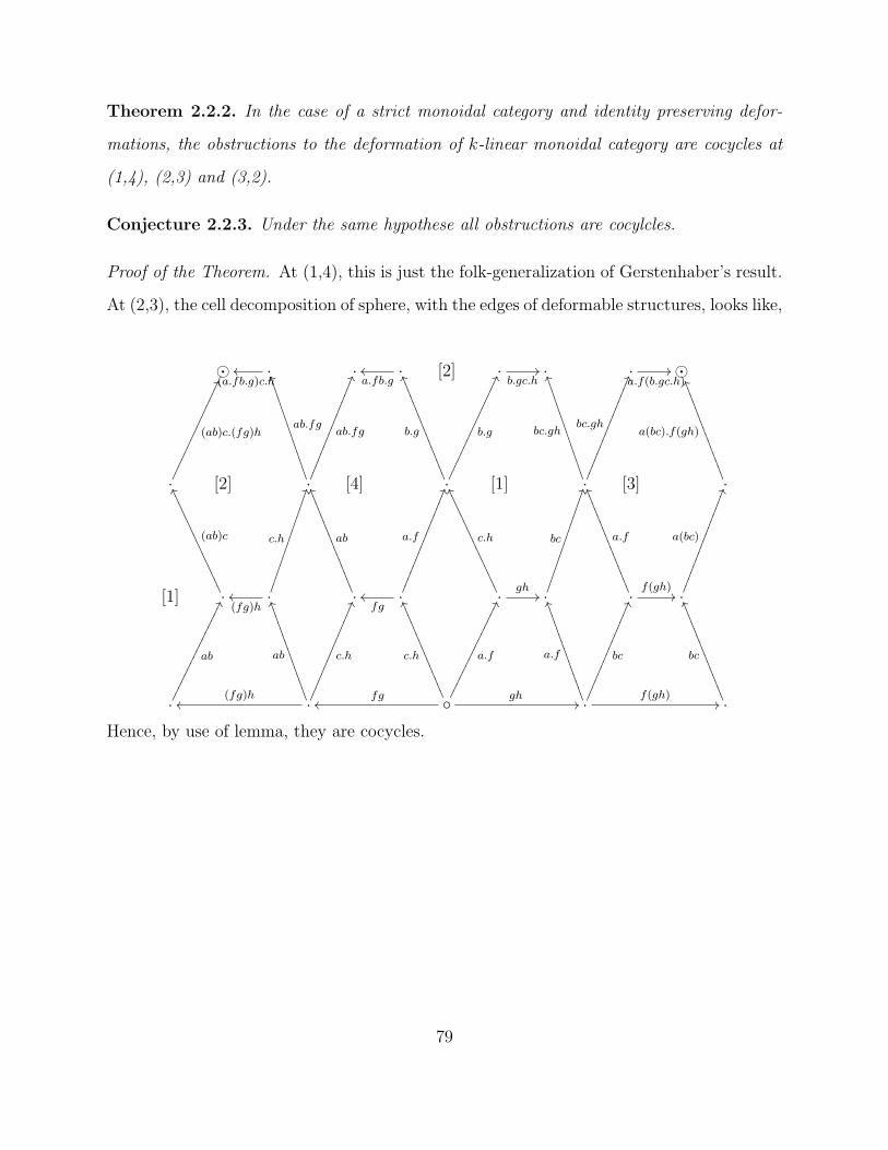
Theorem 2.2.2. In the case of a strict monoidal category and identity preserving defor-

mations, the obstructions to the deformation of k-linear monoidal category are cocycles at

(1,4), (2,3) and (3,2).

Conjecture 2.2.3. Under the same hypothese all obstructions are cocylcles.

Proof of the Theorem. At (1,4), this is just the folk-generalization of Gerstenhaber’s result.

At (2,3), the cell decomposition of sphere, with the edges of deformable structures, looks like,

.(a.fb.g)c.hoo . .

a.fb.goo [2] .

b.gc.h// . .

a.f(b.gc.h)//

.

(ab)c.(fg)h

HH[2] .

ab.fg

UU***************

ab.fg

HH[4] .

b.g

VV,,,,,,,,,,,,,,,,

b.g

HH[1] .

bc.gh

UU***************

bc.gh

HH[3] .

a(bc).f(gh)

UU+++++++++++++++

[1] .

(ab)c

VV.................

(fg)hoo

c.h

II .

ab

VV,,,,,,,,,,,,,,,,.

fgoo

a.f

HH . gh//

c.h

VV.................

bc

II .

a.f

VV,,,,,,,,,,,,,,,, f(gh)// .

a(bc)

II

.

ab

GG .

ab

UU+++++++++++++++

c.h

HH(fg)hoo

c.h

VV---------------

a.f

GGfgoo

gh// .

bc

HH

a.f

UU+++++++++++++++ f(gh)// .

bc

VV,,,,,,,,,,,,,,,

Hence, by use of lemma, they are cocycles.

79

At (3,2), the cell decomposition of sphere, with the edges of deformable structures, looks like,

g.l

ab

++WWWWWWWWWWWWWWWWWWWW .fg

// .

fg.kl

.g.l

kl

22eeeeeeeeeeeeeeeeeeeeeeeeeeeeee

.f.k

,,ZZZZZZZZZZZZZZZZZZZZZZZZZZZZZZ .

αABC

.

f.kg.l33gggggggggggggggggggg

αABC. ab

22dddddddddddddddddddddddddddddd

αABC ''OOOOOOOOOO .

f.kg.l ++WWWWWWWWWWWWWWWWWWWW

.

f.k33gggggggggggggggggggg

ab

;;vvvvvvvvvvvvvvvvvvvvvvvv

a.k

.a.(f.k)

''OOOOOOOOOOab

33gggggggggggggggggggg .ab.(fg.kl).

a.(f.k)αABC

b.(g.l)

''OOOOOOOOOO .

αABCab.(fg.kl)

.

b.(g.l) ''OOOOOOOOOO .αABCa.(f.k)

a.(f.k)b.(g.l)

33gggggggggggggggggggg

. a.(f.k)αABC

33gggggggggggggggggggg

b.(g.l)

''NNNNNNNNNNNNNNNNNNNNNN .

[αABCa.(f.k)]b.(g.l)

''NNNNNNNNNNNNNNNNNNNNN

.αABC

77oooooooooo

.

(a.f)k88pppppppppp

b.(g.l)

&&NNNNNNNNNN .

(a.f).kαUVW

@@

αUVW b.(g.l)

>>>>>>>>>>>>>

.αUVW

''OOOOOOOOOO

.

αUVW b.(g.l)

77ppppppppppppppppppppppαUVW b.(g.l)

++WWWWWWWWWWWWWWWWWWWW .

(a.f).k[αUVW b.(g.l)]

77ppppppppppppppppppppp

.

(a.f).k77oooooooooo

(b.g).lαXY Z

OO

(a.f).k(b.g).l

++WWWWWWWWWWWWWWWWWWWW

.(b.g).lαXY Z

OO

(a.f).k

77oooooooooo .

(ab.fg).klαXY Z

OO

.

b.g ++WWWWWWWWWWWWWWWWWWWW

k.l

##HHHHHHHHHHHHHHHHHHHHHHHH

g.l

OO

. (b.g).l

77oooooooooo

kl ++WWWWWWWWWWWWWWWWWWWW .(ab.fg).kl

OO

.

kl ,,ZZZZZZZZZZZZZZZZZZZZZZZZZZZZZZ

αXY Z77oooooooooo .

a.fb.g33gggggggggggggggggggg

.

a.fb.g ++WWWWWWWWWWWWWWWWWWWWαXY Z

OO

. b.g

22dddddddddddddddddddddddddddddd .

αXY Z

OO

.a.f

OO

ab

,,YYYYYYYYYYYYYYYYYYYYYYYYYYYYYY

a.f

OO

kl

33gggggggggggggggggggg . fg// .

ab.fg

OO

80

To prove the conjecture,at(4,1), the cell decomposition of sphere will be the blown up

version of,

.

αABC.D

$$JJJJJJJJJJJJJJJJJJJJJJJJJJJJJJJJ

(a,f,k.m)L

αA.BCD

::ttttttttttttttttttttttttttttttt

αABC⊗D

7777777777777777777777

(a,f,k,m)L

.

(a,f,k,m)R

.αAB.CD

//

(a,f.k,m)L

.

A⊗αBCD

CC

(a,f.k,m)R

.

αXY Z.W

$$JJ

JJ

JJ

JJ

JJ

JJ

JJ

JJ

.

αX.Y ZW

::tt

tt

tt

tt

tt

tt

tt

tt

αXY Z⊗W

7777777777777777777777 •

.αXY.ZW

// .

X⊗αY ZW

CC

81

and at (5,0), it will be the blown up version of ‘The Stasheff polytope’ with edges the

deformable structures on its edges

.

A⊗αB,C,DE

((PPPPPPPPPPPPPPPPPPPPPPPPPPPPPPPPPPPPPP

.

αA,BC,DE

66nnnnnnnnnnnnnnnnnnnnnnnnnnnnnnnnnnnnnn

.

αA,B,C⊗DE

XX111111111111111111 αAB,C,DE//.

A⊗αBC,D,E

OO

A⊗(αB,C,D⊗E)

1

11

11

11

11 .

αA,B,C(DE)

FF

.

αA(BC),D,E

JJ αA,BC,D⊗E//__________________ .

αA,(BC)D,E

FF

(A⊗αB,C,D)⊗E

1

11

11

11

11 .

A⊗αB,CD,E//__________________ .

A⊗(B⊗αC,D,E)

TT))))))))))))))))))))))))))))))))

αA,BC,D⊗E

JJ

(αA,B,C⊗D)⊗E

XX11111111111111111

αAB,C,D⊗E

((QQQQQQQQQQQQQQQQQQQQQQQQQQQQQQQQQQQQQ .

αA,B(CD),E

FF

.

(AB)⊗αC,D,E

TT)))))))))))))))))))))))))))))))))

αA,B,(CD)E

EE

.

αA,B,CD⊗E

OO

αAB,CD,E

66mmmmmmmmmmmmmmmmmmmmmmmmmmmmmmmmmmmmmm .

82

2.3 Conclusion

1. The deformations of identity functor and natural transformation are classified up to

equivalence by H2(C), that of composition, arrow part of tensor,and that of associator

are classified up to equivalence by H3(C).

2. The obstructions to the deformation of a k-linear monoidal category are 4-cocycles in

special cases.

Conjecture 2.3.1. There are higher homotopy differentials which have the structure of a

multicomplex.

Conjecture 2.3.2. All obstructions are cocycles without additional hypothesis.

83

Bibliography

[1] M. Gerstenhaber, The Cohomology Structure on an Associative Ring, volume 78, 267-

288, Annals of Mathematics, 1963.

[2] M. Gerstenhaber, On the Deformation of Rings and Algebras, volume 79, 59-103,

Annals of Mathematics, 1964.

[3] G. Hochschild, On the Cohomology Gropus of an Associative Algebra, volume 46, No.

1, 58-66, Annals of Mathematics, 1945.

[4] T. F. Fox, An Intoduction to Algebraic Deformation Theory, volume 84, 17-41, Journal

of Pure and Applied Algebra, 1993.

[5] M. Gerstenhaber and S. Schack, Algebras, Bialgebras, Quantum Groups, and Algebraic

Deformations, volume 134, 51-92, Contemporary Mathematics, 1992.

[6] P. Cartier, Cohomologie des Caoalgebras, volume 4 and 5, Seminaire Sophus Lie, 1956.

[7] M. Markl and S. Shnider, Drinfel’d Algebra Deformations, Homotopy Comodules and

the Associahedra, volume 348, 3505-3547., Trans. Amer. Math. Soc., 1996.

[8] C. A. Weibel, An Introduction to Homological Algebra, Cambridge University Press,

2nd Ed, 1997.

[9] D. N. Yetter, Functorial Knot Theory, World Scientific, 1st Ed, 2001.

[10] B. Tsygan, Deformation Quantization of Gerbes, Unpublished Lecture at University

of Pennsylvania, March 6, 2006.

[11] D. N. Yetter, On the Deformation of Pasting Diagrams, volume 22, 24-53., Theory

and Application of Categories, 2009.

84

[12] S. MacLane, Categories for Working Mathematician, Springer-Verlag NY, 2nd Ed,

1971.

[13] P. Etingof, D. Nikshych, and V. Ostrik, On Fusion Categories, volume 162, 581-642,

Annals of Mathematics, 2005.

85

Appendix A

Appendix: Some hand calculations

For brevity we omit the padded composition marks throughout. Every term in the calcula-

tions which follow should be understood as a padded composition.

The cocycle condition of obstruction at (4,1) if tensor and associator only are deformed:

Proof. d0(ω(1)p )(a, f, k,m)

= [a, f, k,m]Lω(1)p (X, Y, Z,W )− ω(1)

p (A,B,C,D)[a, f, k,m]R

= [a, f, k,m]L[α(1)XY Z ⊗ 1Wα

(1)XY.ZW + α

(1)XY Z ⊗ 1W1X ⊗ α(1)

Y ZW

+ α(1)XY.ZW1X ⊗ α(1)

Y ZW − α(1)X.Y ZWα

(1)XY Z.W

+ τ (1)(α(1)XY Z , 1W ) + τ (1)(1X , α

(1)Y ZW )]

− [α(1)ABC ⊗ 1Dα

(1)AB.CD + α

(1)ABC ⊗ 1D1A ⊗ α(1)

BCD

+ α(1)AB.CD1A ⊗ α(1)

BCD − α(1)A.BCDα

(1)ABC.D

+ τ (1)(α(1)ABC , 1D) + τ (1)(1A, α

(1)BCD)][a, f, k,m]R

= α(1)ABC ⊗ 1D[a, f.k,m]Lα

(1)XY.ZW + τ (1)(a, f.k)⊗mα(1)

XY.ZW

+ a.τ (1)(f, k)⊗mα(1)XY.ZW − τ (1)(a.f, k)⊗mα(1)

XY.ZW

− τ (1)(a, f).k ⊗mα(1)XY.ZW + α

(1)ABC ⊗ 1D[a, f.k,m]L1X ⊗ α(1)

Y ZW

+ τ (1)(a, f.k)⊗m1X ⊗ α(1)Y ZW + a.τ (1)(f, k)⊗m1X ⊗ α(1)

Y ZW

− τ (1)(a.f, k)⊗m1X ⊗ α(1)Y ZW − τ (1)(a, f).k ⊗m1X ⊗ α(1)

Y ZW

86

+ α(1)AB.CD[a, f.k,m]R1X ⊗ α(1)

Y ZW + τ (1)(a, f.k ⊗m)1X ⊗ α(1)Y ZW

+ a⊗ τ (1)(f.k,m)1X ⊗ α(1)Y ZW − τ (1)(a⊗ f.k,m)1X ⊗ α(1)

Y ZW

− τ (1)(a, f.k)⊗m1X ⊗ α(1)Y ZW − α

(1)A.BCD[a.f, k,m]Lα

(1)XY Z.W

− τ (1)(a.f, k ⊗m)α(1)XY Z.W − a.f ⊗ τ (1)(k,m)α

(1)XY Z.W

+ τ (1)(a.f, k)⊗mα(1)XY Z.W + τ (1)(a.f ⊗ k,m)α

(1)XY Z.W

− α(1)ABC ⊗ 1Dτ

(1)(a, f.k)⊗m− α(1)ABC ⊗ 1Dτ

(1)(a⊗ f.k,m)

− α(1)ABC ⊗ 1D[a, f.k,m]Rα

(1)XY.ZW + α

(1)ABC ⊗ 1Dτ

(1)(a, f.k ⊗m)

+ α(1)ABC ⊗ 1Da⊗ τ (1)(f.k,m)− α(1)

ABC ⊗ 1Da⊗ τ (1)(f.k,m)


(1)(a, f.k ⊗m)− α(1)ABC ⊗ 1Da⊗ [τ (1)(f, k)⊗m]

− α(1)ABC ⊗ 1D[a, f.k,m]R1X ⊗ α(1)

Y ZW + α(1)ABC ⊗ 1Dτ

(1)(a, f.k ⊗m)

+ α(1)ABC ⊗ 1Da⊗ τ (1)(f.k,m) + α

(1)ABC ⊗ 1Da⊗ [τ (1)(f, k).m]

− α(1)AB.CDa⊗ τ (1)(f.k,m)− α(1)

AB.CDτ(1)(a, f.k ⊗m)

− α(1)AB.CDa⊗ [τ (1)(f, k)⊗m]− α(1)

AB.CD[a, f.k,m]R1X ⊗ α(1)Y ZW

+ α(1)AB.CDτ

(1)(a, f.k ⊗m) + α(1)AB.CDa⊗ τ (1)(f.k,m)

+ α(1)AB.CDa⊗ [τ (1)(f, k).m] + α

(1)A.BCDτ

(1)(a, f)⊗ k.m

+ α(1)A.BCDτ

(1)(a⊗ f,⊗k.m) + α(1)A.BCD[a, f, k.m]α

(1)XY Z.W

− α(1)A.BCDτ

(1)(a, f ⊗ k.m)− α(1)A.BCDa⊗ τ (1)(f, k.m)

+ τ (1)(a.f ⊗ kα(1)XY Z ,m)− τ (1)(a.f ⊗ k,m)α

(1)XY Z ⊗ 1W

+ τ (1)(a, f.k ⊗mα(1)Y ZW )− τ (1)(a, f.k ⊗m)1X ⊗ α(1)

Y ZW

− τ (1)(α(1)ABCa⊗ f.k,m) + α

(1)ABC ⊗ 1Dτ

(1)(a⊗ f.k,m)

− τ (1)(a, α(1)BCDf ⊗ k.m) + 1A ⊗ α(1)

BCDτ(1)(a, f ⊗ k.m)


(1)XY.ZW + τ (1)(a, f.k)⊗mα(1)

XY.ZW


XY.ZW

− τ (1)(a, f).k ⊗mα(1)XY.ZW + α

(1)ABC ⊗ 1D[a, f.k,m]L1X ⊗ α(1)

Y ZW


Y ZW


Y ZW

87

+ α(1)AB.CD[a, f.k,m]R1X ⊗ α(1)

Y ZW + τ (1)(a, f.k ⊗m)1X ⊗ α(1)Y ZW


Y ZW

− τ (1)(a, f.k)⊗m1X ⊗ α(1)Y ZW − α


(1)XY Z.W


(1)XY Z.W


(1)XY Z.W


(1)(a, f.k)⊗m− α(1)ABC ⊗ 1Dτ

(1)(a⊗ f.k,m)


(1)XY.ZW + α

(1)ABC ⊗ 1Dτ

(1)(a, f.k ⊗m)

+ α(1)ABC ⊗ 1Da⊗ τ (1)(f.k,m)− α(1)

ABC ⊗ 1Da⊗ τ (1)(f.k,m)


(1)(a, f.k ⊗m)− α(1)ABC ⊗ 1Da⊗ [τ (1)(f, k)⊗m]

− α(1)ABC ⊗ 1D[a, f.k,m]R1X ⊗ α(1)


(1)(a, f.k ⊗m)

+ α(1)ABC ⊗ 1Da⊗ τ (1)(f.k,m) + α

(1)ABC ⊗ 1Da⊗ [τ (1)(f, k).m]

− α(1)AB.CDa⊗ τ (1)(f.k,m)− α(1)


− α(1)AB.CDa⊗ [τ (1)(f, k)⊗m]− α(1)


+ α(1)AB.CDτ

(1)(a, f.k ⊗m) + α(1)AB.CDa⊗ τ (1)(f.k,m)

+ α(1)AB.CDa⊗ [τ (1)(f, k).m] + α

(1)A.BCDτ

(1)(a, f)⊗ k.m

+ α(1)A.BCDτ

(1)(a⊗ f,⊗k.m) + α(1)A.BCD[a, f, k.m]α

(1)XY Z.W

− α(1)A.BCDτ

(1)(a, f ⊗ k.m)− α(1)A.BCDa⊗ τ (1)(f, k.m)

+ τ (1)(a.f ⊗ kα(1)XY Z ,m)− τ (1)(α

(1)ABCa⊗ f.k,m)

+ τ (1)(a, f.k ⊗mα(1)Y ZW )− τ (1)(a, α

(1)BCDf ⊗ k.m)

− τ (1)(a.f ⊗ k,m)α(1)XY Z ⊗ 1W − τ (1)(a, f.k ⊗m)1X ⊗ α(1)

Y ZW

+ α(1)ABC ⊗ 1Dτ

(1)(a⊗ f.k,m) + 1A ⊗ α(1)BCDτ

(1)(a, f ⊗ k.m)

88


(1)XY.ZW + τ (1)(a, f.k)⊗mα(1)

XY.ZW


XY.ZW

− τ (1)(a, f).k ⊗mα(1)XY.ZW + α

(1)ABC ⊗ 1D[a, f.k,m]L1X ⊗ α(1)

Y ZW


Y ZW


Y ZW

+ α(1)AB.CD[a, f.k,m]R1X ⊗ α(1)

Y ZW + τ (1)(a, f.k ⊗m)1X ⊗ α(1)Y ZW


Y ZW

− τ (1)(a, f.k)⊗m1X ⊗ α(1)Y ZW − α


(1)XY Z.W


(1)XY Z.W


(1)XY Z.W


(1)(a, f.k)⊗m− α(1)ABC ⊗ 1Dτ

(1)(a⊗ f.k,m)


(1)XY.ZW + α

(1)ABC ⊗ 1Dτ

(1)(a, f.k ⊗m)

+ α(1)ABC ⊗ 1Da⊗ τ (1)(f.k,m)− α(1)

ABC ⊗ 1Da⊗ τ (1)(f.k,m)


(1)(a, f.k ⊗m)− α(1)ABC ⊗ 1Da⊗ [τ (1)(f, k)⊗m]

− α(1)ABC ⊗ 1D[a, f.k,m]R1X ⊗ α(1)


(1)(a, f.k ⊗m)

+ α(1)ABC ⊗ 1Da⊗ τ (1)(f.k,m) + α

(1)ABC ⊗ 1Da⊗ [τ (1)(f, k).m]

− α(1)AB.CDa⊗ τ (1)(f.k,m)− α(1)


− α(1)AB.CDa⊗ [τ (1)(f, k)⊗m]− α(1)


+ α(1)AB.CDτ

(1)(a, f.k ⊗m) + α(1)AB.CDa⊗ τ (1)(f.k,m)

+ α(1)AB.CDa⊗ [τ (1)(f, k).m] + α

(1)A.BCDτ

(1)(a, f)⊗ k.m

+ α(1)A.BCDτ

(1)(a⊗ f,⊗k.m) + α(1)A.BCD[a, f, k.m]α

(1)XY Z.W

− α(1)A.BCDτ

(1)(a, f ⊗ k.m)− α(1)A.BCDa⊗ τ (1)(f, k.m)

+ τ (1)(a.τ (1)(f, k),m) + τ (1)(τ (1)(a, f.k),m)

− τ (1)(τ (1)(a, f).k,m)− τ (1)(τ (1)(a.f, k),m)

+ τ (1)(a, τ (1)(f, k ⊗m)) + τ (1)(a, f ⊗ τ (1)(k,m))

− τ (1)(a, τ (1)(f, k).m)− τ (1)(a, τ (1)(f.k,m))


Y ZW

89

+ α(1)ABC ⊗ 1Dτ

(1)(a⊗ f.k,m) + 1A ⊗ α(1)BCDτ

(1)(a, f ⊗ k.m)

90

d1(ω(1)N )(a, f, k,m) = a⊗ ω(1)

N (f, k,m)− ω(1)N (a⊗ f, k,m)

+ ω(1)N (a, f ⊗ k,m)− ω(1)

N (a, f, k ⊗m) + ω(1)N (a, f, k)⊗m

= a⊗ [α(1)BCDτ

(1)(f, k.m) + α(1)BCDf ⊗ τ (1)(k,m) + τ (1)(f, τ (1)(k,m))

− τ (1)(f.k,m)α(1)Y ZW − τ (1)(f, k).mα

(1)Y ZW − τ (1)(τ (1)(f, k),m)]

− [α(1)A.BCDτ

(1)(a.f, k ⊗m) + α(1)A.BCDa.f ⊗ τ (1)(k,m) + τ (1)(a.f, τ (1)(k,m))

− τ (1)(a.f ⊗ k,m)α(1)X.Y ZW − τ (1)(a.f, k)⊗mα(1)

X.Y ZW − τ (1)(τ (1)(a.f, k),m)]

+ [α(1)AB.CDτ

(1)(a, f.k ⊗m) + α(1)AB.CDa⊗ τ (1)(f.k,m) + τ (1)(a, τ (1)(f.k,m))

− τ (1)(a⊗ f.k,m)α(1)XY.ZW − τ (1)(a, f.k)⊗mα(1)

XY.ZW − τ (1)(τ (1)(a, f.k),m)]

− [α(1)ABC.Dτ

(1)(a, f ⊗ k.m) + α(1)ABC.Da⊗ τ (1)(f, k.m) + τ (1)(a, τ (1)(f, k.m))

− τ (1)(a⊗ f, k.m)α(1)XY Z.W − τ (1)(a, f)⊗ k.mα(1)

XY Z.W − τ (1)(τ (1)(a, f), k.m)]

+ [α(1)ABCτ

(1)(a, f.k) + α(1)ABCa⊗ τ (1)(f, k) + αABCτ

(1)(a, τ (1)(f, k))

− τ (1)(a.f, k)α(1)XY Z − τ (1)(a, f)⊗ kα(1)

XY Z − τ (1)(τ (1)(a, f), k)]⊗m

91

Now

d0 + d1 = [a.τ (1)(f, k)⊗mα(1)XY.ZW − τ (1)(a.f, k)⊗mα(1)

XY.ZW

− τ (1)(a, f).k ⊗mα(1)XY.ZW + τ (1)(a, f.k)⊗m1X ⊗ α(1)

Y ZW

+ a.τ (1)(f, k)⊗m1X ⊗ α(1)Y ZW − τ (1)(a.f, k)⊗m1X ⊗ α(1)

Y ZW

− τ (1)(a, f).k ⊗m1X ⊗ α(1)Y ZW + τ (1)(a, f.k ⊗m)1X ⊗ α(1)

Y ZW

− τ (1)(a⊗ f.k,m)1X ⊗ α(1)Y ZW − τ (1)(a, f.k)⊗m1X ⊗ α(1)

Y ZW

− a.f ⊗ τ (1)(k,m)α(1)XY Z.W + τ (1)(a.f, k)⊗mα(1)

XY Z.W

+ τ (1)(a.f ⊗ k,m)α(1)XY Z.W − α

(1)ABC ⊗ 1Dτ

(1)(a⊗ f.k,m)

+ α(1)ABC ⊗ 1Dτ

(1)(a, f.k ⊗m) + α(1)ABC ⊗ 1Da⊗ τ (1)(f.k,m)

− α(1)AB.CDa⊗ [τ (1)(f, k)⊗m] + α

(1)AB.CDa⊗ τ (1)(f.k,m)

+ α(1)AB.CDa⊗ [τ (1)(f, k).m] + α

(1)A.BCDτ

(1)(a, f)⊗ k.m

− α(1)A.BCDτ

(1)(a, f ⊗ k.m)− α(1)A.BCDa⊗ τ (1)(f, k.m)

+ τ (1)(a.τ (1)(f, k),m)− τ (1)(τ (1)(a, f).k,m)

+ τ (1)(a, f ⊗ τ (1)(k,m))− τ (1)(a, τ (1)(f, k).m)


Y ZW

+ α(1)ABC ⊗ 1Dτ

(1)(a⊗ f.k,m) + 1A ⊗ α(1)BCDτ

(1)(a, f ⊗ k.m)]

+ a⊗ ω(1)N (f, k,m)− ω(1)

N (a⊗ f, k,m)

+ ω(1)N (a, f ⊗ k,m)− ω(1)

N (a, f, k ⊗m) + ω(1)N (a, f, k)⊗m

+ [a⊗ [α(1)BCDτ

(1)(f, k.m) + α(1)BCDf ⊗ τ (1)(k,m) + τ (1)(f, τ (1)(k,m))

− τ (1)(f, k).mα(1)Y ZW − τ (1)(τ (1)(f, k),m)]

− [α(1)A.BCDa.f ⊗ τ (1)(k,m) + τ (1)(a.f, τ (1)(k,m))

− τ (1)(a.f ⊗ k,m)α(1)X.Y ZW − τ (1)(a.f, k)⊗mα(1)

X.Y ZW ]

+ [α(1)AB.CDτ

(1)(a, f.k ⊗m)− τ (1)(a⊗ f.k,m)α(1)XY.ZW ]

− [α(1)ABC.Dτ

(1)(a, f ⊗ k.m)− τ (1)(a, f)⊗ k.mα(1)XY Z.W − τ (1)(τ (1)(a, f), k.m)]

+ [α(1)ABCa⊗ τ (1)(f, k) + αABCτ

(1)(a, τ (1)(f, k))

− τ (1)(a.f, k)α(1)XY Z − τ (1)(a, f)⊗ kα(1)

XY Z − τ (1)(τ (1)(a, f), k)]⊗m]

92

Using the lower order coboundary conditions, as in the identity

αA.BCD[τ (1)(a, f).k]⊗m = τ (1)(a, f)⊗k.mαX.Y ZW , we can rearrange groups of terms in which

each group will have a factor like dα(1)ABC ⊗ 1D − α(1)

A.BCD + α(1)AB.CD − α

(1)ABC.D + 1A ⊗ α(1)

BCDe

or the same expression on the target pentagon. Hence the obstructions are cocycle at (4,1)

in this case.

93

By-hand calculation for cocycle condition of obstructions at (3,2) if all structures are

deformed (Note: The superscripts in square brackets preceding terms indicate groups of

terms which are cancelled, either simply with like terms of opposite sign or by applying a

lower order relation.):

Proof. [d0(ω(1)N )− d1(ω

(1)cp )− d2(ω

(1)c )]

(a f kb g l

)= a.f ⊗ kω(1)

N (b, g, l)− ω(1)N (ab, fg, kl)

+ ω(1)N (a, f, k)b⊗ g.l − [ab⊗ ω(1)

cp (f, g; k, l)− ω(1)cp (a⊗ f, k; b⊗ g, l)

+ ω(1)cp (a, f ⊗ k; b, g ⊗ l)− ω(1)

cp (a, f ; b, g)⊗ kl]− [ω(1)c (αABC ; a⊗ f.k; b⊗ g.l)

− ω(1)c (a.f ⊗ k;αUVW ; b⊗ g.l) + ω

(1)c (a.f ⊗ k; b.g ⊗ l;αXY Z)]

= [a.f ⊗ kµ(1)(α(1)UVW , b⊗ g.l) + a.f ⊗ kµ(1)(αUVW , τ

(1)(b, g.l)

+ a.f ⊗ kµ(1)(αUVW , b⊗ g.l) + a.f ⊗ kα(1)UVW τ

(1)(b, g.l)

+ a.f ⊗ kα(1)UVW b⊗ τ (1)g, l) + a.f ⊗ kαUVW τ (1)(b, τ (1)(g, l))

− a.f ⊗ kτ (1)(b, τ (1)(g, l))αXY Z − a.f ⊗ kµ(1)(τ (1)(b.g, l), αXY Z)

− a.f ⊗ kµ(1)(τ (1)(b, g)⊗ l, αXY Z)− a.f ⊗ kµ(1)(b.g ⊗ l, α(1)XY Z)

− a.f ⊗ kτ (1)(b, g)⊗ lα(1)XY Z − a.f ⊗ kτ (1)(b.g, l)α

(1)XY Z ]

− [α(1)ABCτ

(1)(ab, fg ⊗ kl) + µ(1)(α(1)ABC , ab⊗ fg.kl)

+ α(1)ABCab⊗ τ (1)(fg, kl) + µ(1)(αABC , ab⊗ τ (1)(fg, kl))

+ µ(1)(αABC , τ(1)(ab, fg.kl)) + αABCτ

(1)(ab, τ (1)(fg, kl))

− τ (1)(τ (1)(ab, fg), kl)αXY Z − µ(1)(τ (1)(ab, fg)⊗ kl, αXY Z)

− µ(1)(τ (1)(ab.fg, kl), αXY Z)− µ(1)(ab.fg ⊗ kl, α(1)XY Z)

− τ (1)(ab, fg)⊗ α(1)XY Z − τ (1)(ab.fg, kl)α

(1)XY Z ]

+ [µ(1)(α(1)ABC , a⊗ f.kb⊗ g.l) + µ(1)(αABC , τ

(1)(a, f.k))b⊗ g.l

+ µ(1)(αABC , a⊗ τ (1)(f, k))b⊗ g.l + α(1)ABCτ

(1)(a, f.k)b⊗ g.l

+ α(1)ABCa⊗ τ (1)(f, k)b⊗ g.l + αABCτ

(1)(a, τ (1)(f, k))b⊗ g.l

− τ (1)(τ (1)(a, f), k)αUVW b⊗ g.l − µ(1)(τ (1)(a.f, k), αUVW )b⊗ g.l

94

− µ(1)(τ (1)(a, f)⊗ k, αUVW )b⊗ g.l − µ(1)(a.f ⊗ k, α(1)UVW )b⊗ g.l

− τ (1)(a, f ⊗ k)α(1)UVW b⊗ g.l − τ (1)(a.f, k)α

(1)UVW b⊗ g.l]

− αABCab⊗ [τ (1)(f, k)τ (1)(g, l) + µ(1)(τ (1)(f, k), g ⊗ l) + µ(1)(f.k, τ (1)(g, l))

− µ(1)(f, g)⊗ µ(1)(k, l)− τ (1)(µ(1)(f, g), kl)− τ (1)(fg, µ(1)(k, l))]

+ [τ (1)(a.f, k)τ (1)(b, g, l) + µ(1)(τ (1)(a.f, k), b.g ⊗ l) + µ(1)(a.f ⊗ k, τ (1)(b.g, l)

− µ(1)(a.f, b.g)⊗ µ(1)(k, l)− τ (1)(µ(1)(a.f, b.g), kl)

− τ (1)(ab.fg, µ(1)(k, l))]αXY Z

− αABC [τ (1)(a, f.k)τ (1)(b, g.l) + µ(1)(τ (1)(a, f.k), b⊗ g.l)

+ µ(1)(a⊗ f.k, τ (1)(b, g.l))− µ(1)(a, b)⊗ µ(1)(f.k, g.l)

− τ (1)(µ(1)(a, b), fg.kl)− τ (1)(ab, µ(1)(f.k, g.l))]

+ [τ (1)(a, f)τ (1)(b, g) + µ(1)(τ (1)(a, f), b.g)

+ µ(1)(a.f, τ (1)(b, g))− µ(1)(a, b)⊗ µ(1)(f, g)

− τ (1)(µ(1)(a, b), fg)− τ (1)(ab, µ(1)(f, g))]⊗ αXY Z

− µ(1)(µ(1)(αABC , a⊗ f.k), b⊗ g.l) + µ(1)(αABC , µ(1)(a⊗ f.k, b⊗ g.l))

+ µ(1)(µ(1)(a.f ⊗ k, αUVW , b⊗ g.l)− µ(1)(a.f ⊗ k, µ(1)(αUVW , b⊗ g.l))

− µ(1)(µ(1)(a.f ⊗ k, b.g ⊗ l), αXY Z)− µ(1)(a.f ⊗ k, µ(1)(b.g ⊗ l, αXY Z))

=[13] a.f ⊗ kµ(1)(α(1)UVW , b⊗ g.l) + a.f ⊗ µ(1)(αUVW , τ

(1)(b, g.l))

+ a.f ⊗ kµ(1)(αUVW , b⊗ τ (1)(g, l)) + a.f ⊗ kα(1)UVW τ

(1)(b, g.l)

+ a.f ⊗ kα(1)UVW b⊗ τ (1)(g, l) + a.f ⊗ kα(1)

UVW τ(1)(b, τ (1)(g, l))

− a.f ⊗ kτ (1)(b, τ (1)(b, l))αXY Z − a.f ⊗ kµ(1)(τ (1)(b, g.l), αXY Z)

− a.f ⊗ kµ(1)(τ (1)(b, g)⊗ l, αXY Z)−[11] a.f ⊗ kµ(1)(b.g ⊗ l, αXY Z)

−[5] a.f ⊗ kµ(1)(b, g)⊗ l, αXY Z)−[4] a.f ⊗ kτ (1)(b.g, l)αXY Z)

−[7] α(1)ABCτ

(1)(a, f.k)τ (1)(b, g.l)−[12] α(1)ABCµ

(1)(a⊗ f.k, b⊗ g.l)

− α(1)ABCa⊗ f.kτ (1)(b, g.l) + α

(1)ABCµ

(1)(a, b)⊗ fg.kl

+[1] α(1)ABCab⊗ µ(1)(f.k, g.l)−[12] µ(1)(α

(1)ABC , a⊗ f.kb⊗ g.l)

− µ(1)(αABC , τ(1)(a, f.k)b⊗ g.l)−[2] µ(1)(αABC , µ

(1)(a⊗ f.k, b⊗ g.l))

95

− µ(1)(αABC , a⊗ f.kτ (1)(b, g.l)) + µ(1)(αABC , µ(1)(a, b)⊗ fg.kl)

+[9] µ(1)(αABC , ab⊗ µ(1)(f.k, g.l))− µ(1)(αABC , a⊗ τ (1)(f, k)b⊗ g.l)

−[9] µ(1)(α(1)ABC , ab⊗ µ(1)(f.k, g.l))− µ(1)(αABC , a⊗ f.kb⊗ τ (1)b, l)

+ µ(1)(αABC , ab⊗ µ(1)(f, g)kl) + µ(1)(αABC , ab⊗ fg.µ(1)(k, l))

−[8] α(1)ABCab⊗ τ (1)(f, k)g.l − α(1)

ABCab⊗ (f.kτ (1)(g, l))

−[1] α(1)ABCab⊗ µ(1)(f.k, g.l)− α(1)

ABCab⊗ µ(1)(f, g).kl

+ α(1)ABCab⊗ fg.µ(1)(k, l)− αABCτ (1)(ab, τ (1)(f, k)g.l)

− αABCτ (1)(ab, µ(1)(f.k, g.l)− αABCτ (1)(ab, f.kτ (1)(g, l))

+ αABCτ(1)(ab, µ(1)(f, g).kl) + αABCτ

(1)(ab, fg.µ(1)(k, l))

+ τ (1)(τ (1)(a, f)b.g, kl)αXY Z + τ (1)(a.fτ (1)(b, g), kl)αXY Z

+ τ (1)(µ(1)(a.f, b.g), kl)αXY Z − τ (1)(µ(1)(a, b).fg, kl)αXY Z

− τ (1)(ab.µ(1)(f, g), kl)αXY Z + µ(1)(τ (1)(a, f)b.g ⊗ kl, αXY Z)

+ µ(1)(a.fτ (1)(b, g)⊗ kl, αXY Z) +[10] µ(1)(µ(1)(a.f, b.g)⊗ kl, αXY Z)

− µ(1)(µ(1)(a, b).fg ⊗ kl, αXY Z)− µ(1)(ab.µ(1)(f, g)⊗ kl, αXY Z)

+ µ(1)(τ (1)(a.f, k)b.g ⊗ l, αXY Z) + µ(1)(a.f ⊗ kτ (1)(b.g, l), αXY Z)

+[3] µ(1)(µ(1)(a.f ⊗ k, b.g ⊗ l), αXY Z)−[10] µ(1)(µ(1)(a.f, b.g)⊗ kl, αXY Z)

− µ(1)(ab, fg)⊗ µ(1)(k, l)αXY Z + µ(1)(a.f ⊗ kb.g ⊗ l, α(1)XY Z)

+ τ (1)(a, f)b.g ⊗ klα(1)XY Z +[6] µ(1)(a.f, b.g)⊗ klα(1)

XY Z

+[5] a.fτ (1)(b, g)⊗ klα(1)XY Z − µ(1)(a, b).fg ⊗ klα(1)

XY Z

− ab.µ(1)f, g)⊗ klα(1)XY Z + τ (1)(a.f, k)b.g ⊗ lα(1)

XY Z

+[4] a.f ⊗ kτ (1)(b.g, l)α(1)XY Z +[11] µ(1)(a.f ⊗ k, b.g ⊗ l)α(1)

XY Z

−[6] µ(1)(a.f, b.g)⊗ klα(1)XY Z − ab.fg ⊗ µ(1)(k, l)α

(1)XY Z

+[12] µ(1)(α(1)ABC , a⊗ f.kb⊗ g.l) +[7] α

(1)ABCτ

(1)(a, f.k)b⊗ g.l

+[8] α(1)ABCa⊗ f.kτ (1)(b, g.l) + µ(1)(αABC , τ

(1)(a, f.k))b⊗ g.l

+ µ(1)(αABC , a⊗ τ (1)(f, k))b⊗ g.l + αABCτ(1)(a, τ (1)(f, k))b⊗ g.l

− τ (1)(τ (1)(a, f), k)αUVW b⊗ g.l − µ(1)(τ (1)(a, f)⊗ k, αUVW )b⊗ g.l

−[13] µ(1)(a.f ⊗ k, α(1)UVW )b⊗ g.l − τ (1)(a.f, k)α

(1)UVW )b⊗ g.l

96

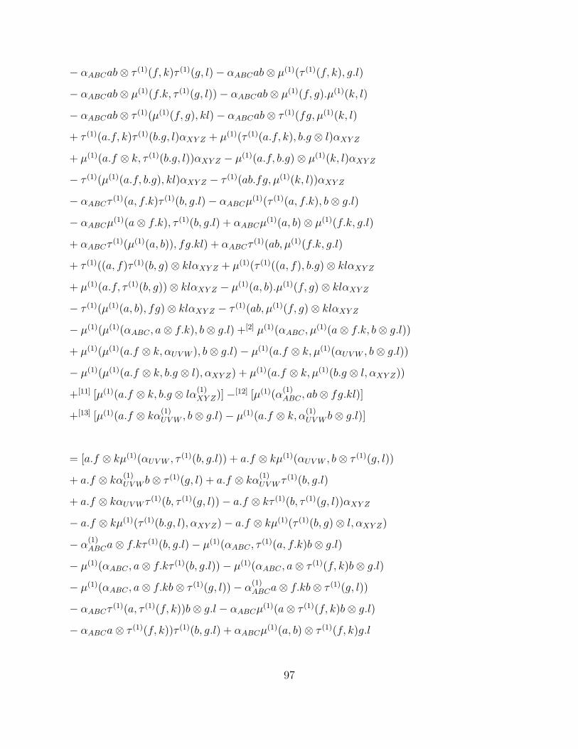
− αABCab⊗ τ (1)(f, k)τ (1)(g, l)− αABCab⊗ µ(1)(τ (1)(f, k), g.l)

− αABCab⊗ µ(1)(f.k, τ (1)(g, l))− αABCab⊗ µ(1)(f, g).µ(1)(k, l)

− αABCab⊗ τ (1)(µ(1)(f, g), kl)− αABCab⊗ τ (1)(fg, µ(1)(k, l)

+ τ (1)(a.f, k)τ (1)(b.g, l)αXY Z + µ(1)(τ (1)(a.f, k), b.g ⊗ l)αXY Z

+ µ(1)(a.f ⊗ k, τ (1)(b.g, l))αXY Z − µ(1)(a.f, b.g)⊗ µ(1)(k, l)αXY Z

− τ (1)(µ(1)(a.f, b.g), kl)αXY Z − τ (1)(ab.fg, µ(1)(k, l))αXY Z

− αABCτ (1)(a, f.k)τ (1)(b, g.l)− αABCµ(1)(τ (1)(a, f.k), b⊗ g.l)

− αABCµ(1)(a⊗ f.k), τ (1)(b, g.l) + αABCµ(1)(a, b)⊗ µ(1)(f.k, g.l)

+ αABCτ(1)(µ(1)(a, b)), fg.kl) + αABCτ

(1)(ab, µ(1)(f.k, g.l)

+ τ (1)((a, f)τ (1)(b, g)⊗ klαXY Z + µ(1)(τ (1)((a, f), b.g)⊗ klαXY Z

+ µ(1)(a.f, τ (1)(b, g))⊗ klαXY Z − µ(1)(a, b).µ(1)(f, g)⊗ klαXY Z

− τ (1)(µ(1)(a, b), fg)⊗ klαXY Z − τ (1)(ab, µ(1)(f, g)⊗ klαXY Z

− µ(1)(µ(1)(αABC , a⊗ f.k), b⊗ g.l) +[2] µ(1)(αABC , µ(1)(a⊗ f.k, b⊗ g.l))

+ µ(1)(µ(1)(a.f ⊗ k, αUVW ), b⊗ g.l)− µ(1)(a.f ⊗ k, µ(1)(αUVW , b⊗ g.l))

− µ(1)(µ(1)(a.f ⊗ k, b.g ⊗ l), αXY Z) + µ(1)(a.f ⊗ k, µ(1)(b.g ⊗ l, αXY Z))

+[11] [µ(1)(a.f ⊗ k, b.g ⊗ lα(1)XY Z)]−[12] [µ(1)(α

(1)ABC , ab⊗ fg.kl)]

+[13] [µ(1)(a.f ⊗ kα(1)UVW , b⊗ g.l)− µ(1)(a.f ⊗ k, α(1)

UVW b⊗ g.l)]

= [a.f ⊗ kµ(1)(αUVW , τ(1)(b, g.l)) + a.f ⊗ kµ(1)(αUVW , b⊗ τ (1)(g, l))

+ a.f ⊗ kα(1)UVW b⊗ τ (1)(g, l) + a.f ⊗ kα(1)

UVW τ(1)(b, g.l)

+ a.f ⊗ kαUVW τ (1)(b, τ (1)(g, l))− a.f ⊗ kτ (1)(b, τ (1)(g, l))αXY Z

− a.f ⊗ kµ(1)(τ (1)(b.g, l), αXY Z)− a.f ⊗ kµ(1)(τ (1)(b, g)⊗ l, αXY Z)

− α(1)ABCa⊗ f.kτ (1)(b, g.l)− µ(1)(αABC , τ

(1)(a, f.k)b⊗ g.l)

− µ(1)(αABC , a⊗ f.kτ (1)(b, g.l))− µ(1)(αABC , a⊗ τ (1)(f, k)b⊗ g.l)

− µ(1)(αABC , a⊗ f.kb⊗ τ (1)(g, l))− α(1)ABCa⊗ f.kb⊗ τ (1)(g, l))

− αABCτ (1)(a, τ (1)(f, k))b⊗ g.l − αABCµ(1)(a⊗ τ (1)(f, k)b⊗ g.l)

− αABCa⊗ τ (1)(f, k))τ (1)(b, g.l) + αABCµ(1)(a, b)⊗ τ (1)(f, k)g.l

97

+ αABCab⊗ µ(1)(τ (1)(f, k), g.l)− αABCτ (1)(ab, µ(1)(f.k, g.l))

− αABCτ (1)(a, f.k)b⊗ τ (1)(g, l)− αABCµ(1)(a⊗ f.k, b⊗ τ (1)(g, l))

− αABCa⊗ f.kτ (1)(b, τ (1)(g, l)) + αABCµ(1)(a, b)⊗ f.kτ (1)(g, l)

+ αABCab⊗ µ(1)(f.k, τ (1)(g, l)) + τ (1)(τ (1)(a, f), k)b.g ⊗ lαXY Z

+ µ(1)(τ (1)(a, f)⊗ k, b.g ⊗ l)αXY Z + τ (1)(a, f)⊗ kτ (1)(b.g, l)αXY Z

− µ(1)(τ (1)(a, f), b.g)⊗ klαXY Z − τ (1)(a, f)b.g ⊗ µ(1)(k, l)αXY Z

+ τ (1)(a.f, k)τ (1)(b, g)⊗ lαXY Z + a.f ⊗ kτ (1)(τ (1)(b, g), l)αXY Z

+ µ(1)(a.f ⊗ k, τ (1)(b, g)⊗ l)αXY Z − τ (1)(a.f, τ (1), τ (1)(b, g))⊗ klαXY Z

− a.fτ (1)(b, g)⊗ µ(1)(k, l)αXY Z − τ (1)(µ(1)(a.f, b.g), kl)αXY Z

+ µ(1)(τ (1)(a, f)⊗ kb.g ⊗ l, αXY Z) + µ(1)(a.f ⊗ k, τ (1)(b, g)⊗ l, αXY Z)


+ τ (1)(a, f)⊗ kb.g ⊗ lα(1)XY Z + τ (1)(a.f, k)b.g ⊗ lα(1)

XY Z)

+ µ(1)(αABC , τ(1)(a, f.k)b⊗ g.l + µ(1)(αABC , a⊗ τ (1)(f, k)b⊗ g.l


− µ(1)(τ (1)(a, f)⊗ k, αUVW )b⊗ g.l − τ (1)(a, f)⊗ kα(1)UVW b⊗ g.l

− µ(1)(τ (1)(a.f, k), αUVW )b⊗ g.l − τ (1)(a.f, k)α(1)UVW b⊗ g.l

− αABCa⊗ τ (1)(f, k)b⊗ τ (1)(g, l)− αABCab⊗ µ(1)(τ (1)(f, k), g.l)

− αABCab⊗ µ(1)(f.k, τ (1)(g, l)) + τ (1)(a.f, k)τ (1)(b.g, l)αXY Z

+ µ(1)(τ (1)(a.f, k), b.g ⊗ l)αXY Z + µ(1)(a.f ⊗ k, τ (1)(b.g, l))αXY Z

− µ(a.f, b.g)µ(1)(k, l)αXY Z − τ (1)(µ(1)(a.f, b.g), kl)αXY Z

− αABCτ (1)(a, f.k)τ (1)(b, g.l)− αABCµ(1)(τ (1)(a, f.k), b⊗ g.l)

− αABCµ(1)(a⊗ f.k, τ (1)(b, g.l)) + αABCµ(1)(a, b)⊗ µ(1)(f.k, g.l)

+ αABCτ(1)(ab, µ(1)(f.k, g.l) + µ(1)(a.f, τ (1)(b, g))⊗ klαXY Z

− αABCµ(1)(a, b)⊗ µ(1)(f, g).kl + τ (1)(a, f)⊗ kτ (1)(b, g)⊗ lαXY Z

+ µ(1)(τ (1)(a, f), b.g)⊗ klαXY Z + αABCab⊗ µ(1)(f, g).µ(1)(k, l)

− µ(1)(µ(1)(αABC , a⊗ f.k), b⊗ g.l) + µ(1)(µ(1)(a.f ⊗ k, αUVW ), b⊗ g.l)

− µ(1)(a.f ⊗ k, µ(1)(αUVW , b⊗ g.l)) + µ(1)(a.f ⊗ k, µ(1)(b⊗ g.l, αXY Z)

98

+ µ(1)(a.f ⊗ kb⊗ g.l), α(1)XY Z)− µ(1)(α

(1)ABC , a⊗ f, kb⊗ g.l)

+ µ(1)(a.f ⊗ kα(1)UVW , b⊗ g.l)− µ(1)(a.f ⊗ k, α(1)

UVW b⊗ g.l)

− αABCµ(1)(a, b)⊗ τ (1)(fg, kl) + τ (1)(ab, fg)⊗ µ(1)(k, l)αXY Z

= a.f ⊗ kµ(1)(αUVW , τ(1)(b, g.l) + a.f ⊗ kµ(1)(αUVW , b⊗ τ (1)(g, l))

+[7] a.f ⊗ kαUVW τ (1)(b, τ (1)(g, l))−[8] a.f ⊗ kτ (1)(τ (1)(b, g), l)αXY Z

− a.f ⊗ kµ(1)(τ (1)(b.g, l), αXY Z)− a.f ⊗ kµ(1)(τ (1)(b, g)⊗ l, αXY Z)

− µ(1)(αABC , τ(1)(a, f.k)b⊗ g.l)− µ(1)(αABC , a⊗ f.kτ (1)(b, g.l))

− µ(1)(αABC , a⊗ τ (1)(f, k)b⊗ g.l)− µ(1)(αABC , a⊗ f.kb⊗ τ (1)(g, l))

−[6] αABCτ(1)(a, τ (1)(f, k))b⊗ g.l − αABCµ(1)(a⊗ τ (1)(f, k), b⊗ g.l)

−[10] αABCa⊗ τ (1)(f, k)τ (1)(b, g.l) + αABCµ(1)(a, b)⊗ τ (1)(f, k)g.l

+[22] αABCab⊗ µ(1)(f, k), g.l)−[27] τ (1)(ab, µ(1)(f.k, g.l))

−[13] αABCτ(1)(a, f.k)b⊗ τ (1)g, l)− αABCµ(1)(a⊗ f.k, b⊗ τ (1)(g, l))

−[7] αABCa⊗ f.kτ (1)(b, τ (1)(g, l)) + αABCµ(1)(a, b)⊗ f.kτ (1)(g, l)

+[11] αABCab⊗ µ(1)(f.k, τ (1)(g, l)) + [5]τ (1)τ (1)(a, f), k)b.g ⊗ lαXY Z

+ µ(1)(τ (1)(a, f)⊗ k, b.g ⊗ l)αXY Z +[23] τ (1)(a, f)⊗ kτ (1)(b.g, l)αXY Z

−[21] µ(1)(τ (1)(a, f), b.g)⊗ klαXY Z − τ (1)(a, f)b.g ⊗ µ(1)(k, l)αXY Z

+[25] τ (1)(a.f, k)τ (1)(b, g)⊗ lαXY Z +[8] a.f ⊗ kτ (1)(τ (1)(b, g), k)αXY Z

+ µ(1)(a.f ⊗ k, τ (1)(b, g)⊗ l)αXY Z −[20] µ(1)(a.f, τ (1)(b, g))⊗ klαXY Z

− a.fτ (1)(b, g)⊗ µ(1)(k, l)αXY Z −[26] τ (1)(µ(1)(a.f, b.g), kl)αXY Z

+ µ(1)(τ (1)(a, f)⊗ kb.g ⊗ l, αXY Z) + µ(1)(a.f ⊗ kτ (1)(b, g)⊗ l, αXY Z)


+ µ(1)(αABC , τ(1)(a, f.k)b⊗ g.l + µ(1)(αABC , a⊗ τ (1)(f, k))b⊗ g.l

+[6] αABCτ(1)(a, tau(1)(f, k))b⊗ g.l −[5] τ (1)(τ (1)(a, f), k)b⊗ g.l

− µ(1)(τ (1)(a, f)⊗ k, αUVW )b⊗ g.l − µ(1)(τ (1)(a.f, k), αUVW )b⊗ g.l

−[9] αABCa⊗ τ (1)(f, k)b⊗ τ (1)(g, l)−[22] αABCab⊗ µ(1)(τ (1)(f, k), g.l)

−[11] αABCab⊗ µ(1)(f.k, τ (1)(g, l)) +[24] τ (1)(a.f, k)τ (1)(b.g, l)αXY Z

99

+ µ(1)(τ (1)(a.f, k), b.g ⊗ l)αXY Z + µ(1)(a.f ⊗ k, τ (1)(b.g, l))αXY Z

− µ(1)(a.f, b.g)µ(1)(k, l)αXY Z −[26] τ (1)(µ(1)(a.f, b.g), kl)αXY Z

−[14] αABCτ(1)(a, f.k(τ (1)(b, g.l)− αABCµ(1)(τ (1)(a, f.k), b⊗ g.l)

− αABCµ(1)(a⊗ f.k, τ (1)(b, g.l)) + αABCµ(1)(a, b).µ(1)(f.k, g.l)

+[27] τ (1)(ab, µ(1)(f.k, g.l)) +[20] µ(1)(a.f, τ (1)(b, g))⊗ klαXY Z

+ [19]τ (1)(a, f)⊗ kτ (1)(b, g)⊗ lαXY Z + [21]µ(1)(τ (1)(a, f), b.g)⊗ klαXY Z

− µ(1)(a, b).µ(1)(f, g)⊗ klαXY Z + α + ABXab⊗ µ(1)(f, g).µ(1)(k, l)

−[3] µ(1)(µ(1)(αABC , a⊗ f.k)b⊗ g.l +[4] µ(1)(µ(1)(a.f ⊗ k, αUVW ), b⊗ g.l)

−[1] µ(1)(a.f ⊗ k, µ(1)(αUVW , b⊗ g.l)) +[2] µ(1)(a.f ⊗ k, µ(1)(b⊗ g.l, αXY Z))

− αABCµ(1)(a, b)µ(1)(fg, kl) + τ (1)(ab, fg)⊗ µ(1)(k, l)αXY Z

+[1] [µ(1)(a.f ⊗ k, b.g ⊗ l)α(1)XY Z − µ(1)(a.f ⊗ k, α(1)

UVW b⊗ g.l)]

+[2] [µ(1)(a.f ⊗ kα(1)UVW , b⊗ g.l)− µ(1)(α

(1)ABCa⊗ f.k, b⊗ g.l)]

+[3] [a.f ⊗ kα(1)UVW τ

(1)(b, g.l)− α(1)ABCa⊗ f.kτ (1)(b, g.l)]

+[4] [a.f ⊗ kα(1)UVW b⊗ τ (1)(g, l)− α(1)

ABCa⊗ f.kb⊗ τ (1)(g, l)]

+[5] [τ (1)(a, f)⊗ b.g ⊗ lα(1)XY Z − τ (1)(a, f)⊗ α(1)

UVW b⊗ g.l]

+[6] [τ (1)(a.f, k)b.g ⊗ lα(1)XY Z − τ (1)(a.f, k)α

(1)UVW b⊗ g.l]

Above last 5 boxes labeled 1,2,..,5, can be written as

+[5][τ (1)(a, f)⊗ b.g ⊗ lα(1)XY Z − τ (1)(a, f)⊗ α(1)

UVW b⊗ g.l]

= τ (1)(a, f)⊗ kµ(1)(αUVW , b⊗ g.l) + τ (1)(a, f)⊗ kτ (1)(b, g.l)

+ τ (1)(a, f)⊗ kαUVW b⊗ τ (1)(g, l)− τ (1)(a, f ⊗ τ (1)(b, g)⊗ lαXY Z

− τ (1)(a, f)⊗ kτ (1)(b.g, l)αXY Z − τ (1)(a, f)⊗ kµ(1)(b.g ⊗ l, αXY Z

and similar expressions for others. So, the last 5 boxes can be replaced by

+[1]µ(1)(a.f ⊗ k, µ(1)(αUVW , b⊗ g.l)) + µ(1)(a.f ⊗ k, αUVW τ (1)(b, g.l)

+ µ(1)(a.f ⊗ k, αUVW b⊗ τ (1)(g, l))− µ(1)(a.f ⊗ k, µ(1)(b.g ⊗ l, αXY Z))

− µ(1)(a.f ⊗ k, τ (1)(b.g, l)αXY Z)−[2] µ(1)(a.f ⊗ k, µ(1)(b.g ⊗ l, αXY Z))

100

+[3] µ(1)(µ(1)(αABC , a⊗ f.k), b⊗ g.l) + µ(1)(αABCτ(1)(a, f.k), b⊗ g.l)

+ µ(1)(αABCa⊗ τ (1)(f, g), b⊗ g.l)− µ(1)(τ (1)(a, f)⊗ kαUVW , b⊗ g.l)

− µ(1)(τ (1)(a.f, k)αUVW , b⊗ g.l)−[4] µ(1)(µ(1)(a.f ⊗ k, αUVW ), b⊗ g.l)

+ µ(1)(αABC , a⊗ f.k)τ (1)(b, g.l) +[14] αABCτ(1)(a, f.k)τ (10(b, g.l)

+[10] αABCa⊗ τ (1)(f, k)τ (1)(b, g.l)−[18] τ (1)(a, f)⊗ kαUVW τ (1)(b, g.l)

−[15] τ (1)(a.f, k)αUVW τ(1)(b, g.l)− µ(1)(a.f ⊗ k, αUVW )τ (1)(b, g.l)

+ µ(1)(αABC , a⊗ f.k)b⊗ τ (1)(g, l) +[13] αABCτ(1)(a, f.k)b⊗ τ (1)(g, l)

+[9] αABCa⊗ τ (1)(f, k)b⊗ τ (1)(g, l)−[16] τ (1)(a, f)⊗ kαUVW b⊗ τ (1)(g, l)

−[17] τ (1)(a.f, k)αUVW b⊗ τ(1)(g, l)− µ(1)(a.f ⊗ k, αUVW )b⊗ τ (1)(g, l)

+ τ (1)(a, f)⊗ kµ(1)(αUVW , b⊗ g.l) +[18] τ (1)(a, f)⊗ kαUVW τ (1)(b, g.l)

+[16] τ (1)(a, f)⊗ kαUVW b⊗ τ (1)(g, l)−[19] τ (1)(a, f)⊗ kτ (1)(b, g)⊗ lαXY Z

−[23] τ (1)(a, f)⊗ kτ (1)(b.g, l)αXY Z − τ (1)(a, f)⊗ kµ(1)(b.g ⊗ l, αXY Z)

+ τ (1)(a.f, k)µ(1)(αUVW , b⊗ g.l) + [15]τ (1)(a.f, k)αUVW τ(1)(b, g.l)

+[17] τ (1)(a.f, k)αUVW b⊗ τ (1)(g, l)− τ (1)(a.f, k)τ (1)(b, g)⊗ lαXY Z

−[24] τ (1)(a.f, k)τ (1)(b.g, l)αXY Z −[25] τ (1)(a.f, k)µ(1)(b.g ⊗ l, αXY Z)

Hence, using the lower order conditions and cancelation of the like terms with opposite

signs, we get,

=[4] a.f ⊗ kµ(1)(αUVW , τ(1)(b, g.l)) +[6] a.f ⊗ kµ(1)(αUVW , b⊗ τ (1)(g, l))

−[5] a.f ⊗ kµ(1)(τ (1)(b.g, l), αXY Z) +[15] a.f ⊗ kµ(1)(b⊗ τ (1)(g, l), αXY Z)

−[8] µ(1)(αABC , τ(1)(a, f.k)b⊗ g.l)−[9] µ(1)(αABC , a⊗ f.kτ (1)(b, g.l))

−[7] µ(1)(αABC , a⊗ τ (1)(f, k)b⊗ g.l)−[14] µ(1)(αABC , a⊗ f, kb⊗ τ (1)(g, l))

−[7]αABCµ(1)(a⊗ τ (1)(f, k), b⊗ g.l)−[14] αABCµ

(1)(a⊗ f.k, b⊗ τ (1)(g, l))

+[10]µ(1)(τ (1)(a, f)⊗ k, b.g ⊗ l)αXY Z

+[15] µ(1)(a.f ⊗ k, τ (1)(b, g)⊗ l)αXY Z

+[10] µ(1)(τ (1)(a, f)⊗ k, b.g ⊗ lαXY Z)

101

+[15] µ(1)(a.f ⊗ kτ (1)(b, g)⊗ l, αXY Z)

+[12] µ(1)(τ (1)(a.f, k)b.g ⊗ l, αXY Z) +[5] µ(1)(a.f ⊗ kτ (1)(b.g, l), αXY Z)

+[8] µ(1)(αABC , τ(1)(a, f.k)b⊗ g.l +[7] µ(1)(αABC , τ

(1)(f, k)b⊗ g.l)

−[11] µ(1)(τ (1)(a, f)⊗ kαUVW )b⊗ g.l −[13] µ(1)(τ (1)(a.f, k), αUVW )b⊗ g.l

+[12]µ(1)(τ (1)(a.f, k), b⊗ g.l)αXY Z +[5] µ(1)(a.f ⊗ k, τ (1)(b.g, l))αXY Z

−[8] αABCµ(1)(τ (1)(a, f.k), b⊗ g.l)−[9] µ(1)(a⊗ f.k, τ (1)(b, g.l))

−[3] µ(1)(a, b).µ(1)(f, g)⊗ klαXY Z +[2] αABCab⊗ µ(1)(f, g).µ(1)(k, l)

+[4] µ(1)(a.f ⊗ k, αUVW τ (1)(b, g.l)) +[6] µ(1)(a.f ⊗ k, αUVW b⊗ τ (g, l))

+[15]µ(1)(a.f ⊗ k, τ (1)(b, g)⊗ lαXY Z) +[5] µ(1)(a.f ⊗ k, τ (1)(b.g, l)αXY Z)

+[8] µ(1)(αABCτ(1)(a, f.k), b⊗ g.l) +[7] µ(1)(αABCa⊗ τ (1)(f, k), b⊗ g.l)

−[11] µ(1)(τ (1)(a, f)⊗ kαUVW , b⊗ g.l) −[13]µ(1)(τ (1)(a.f, k)αUVW )b⊗ g.l

+[9] µ(1)(αABC , a⊗ f.k)τ (1)(b, g.l)−[4] µ(1)(a.f, k, αUVW )τ (1)(b, g.l)

+[14] µ(1)(αABC , a⊗ f.k)b⊗ τ (1)(g, l)−[6] µ(1)(a.f ⊗ k, αXY Z)b⊗ τ (1)(g, l)

+[11] τ (1)(a, f)⊗ kµ(1)(αUVW , b⊗ g.l)−[10] τ (1)a, f)⊗ kµ(1)(b.g ⊗ l, αXY Z)

+[13]τ (1)(a.f, k)µ(1)(αUVW , b⊗ g.l)−[12] τ (1)(a.f, k)µ(1)(b.g ⊗ l, αXY Z)

+[3] αABCµ(1)(a, b)⊗ µ(1)(f, g).kl +[1] αABCµ

(1)(a, b)⊗ fg.µ(1)(k, l)

−[1] µ(1)(a, b).fg ⊗ µ(1)(k, l)αXY Z −[2] ab.µ(1)(f, g)⊗ µ(1)(k, l)αXY Z

+[9][4]µ

(1)(a.f ⊗ kαUVW , τ (1)(b, g.l)) +[11][10] µ

(1)(τ (1)(a.f)⊗ k, b.g ⊗ lαXY Z)

−[13][12] µ

(1)(τ (1)(a.f, k), b.g ⊗ lαXY Z)−[6][14] µ

(1)(αABCa⊗ f.k, τ (1)(b, g.l))

= 0

102

ALGEBRAIC DEFORMATION OF A MONOIDAL CATEGORY by TEJ B. SHRESTHA B

Documents

Transcript of ALGEBRAIC DEFORMATION OF A MONOIDAL CATEGORY by TEJ B. SHRESTHA B