Alexandre d’Aspremont CNRS - ENSaspremon/PDF/Sophia14.pdf · Alexandre d’Aspremont, CNRS - ENS....
54
Optimisation et apprentissage. Alexandre d’Aspremont, CNRS - ENS. A. d’Aspremont INRIA, Apr. 2014 1/52
Transcript of Alexandre d’Aspremont CNRS - ENSaspremon/PDF/Sophia14.pdf · Alexandre d’Aspremont, CNRS - ENS....

Optimisation et apprentissage.
Alexandre d’Aspremont, CNRS - ENS.
A. d’Aspremont INRIA, Apr. 2014 1/52

Introduction
Today. . .
� Focus on convexity and its impact on complexity.
� Convex approximations, duality.
� Applications in learning.
A. d’Aspremont INRIA, Apr. 2014 2/52

Introduction
In optimization.
Twenty years ago. . .
� Solve realistic large-scale problems using naive algorithms.
� Solve small, naive problems using serious algorithms.
Twenty years later. . .
� Solve realistic problems in e.g. statistics, signal processing, using efficientalgorithms with explicit complexity bounds.
� Statisticians have started to care about complexity.
� Optimizers have started to care about statistics.
A. d’Aspremont INRIA, Apr. 2014 3/52

Introduction
Convexity.
Convex Not convex
Key message from complexity theory: as the problem dimension gets large
� all convex problems are easy,
� most nonconvex problems are hard.
A. d’Aspremont INRIA, Apr. 2014 4/52

Introduction
Convex problem.
minimize f0(x)subject to fi(x) ≤ 0, i = 1, . . . ,m
aTi x = bi, i = 1, . . . , p
f0, f1, . . . , fm are convex functions, the equality constraints are all affine.
� Strong assumption, yet surprisingly expressive.
� Good convex approximations of nonconvex problems.
A. d’Aspremont INRIA, Apr. 2014 5/52

Introduction
First-order condition. Differentiable f with convex domain is convex iff
f(y) ≥ f(x) +∇f(x)T (y − x) for all x, y ∈ dom f
(x, f(x))
f(y)
f(x) +∇f(x)T (y − x)
First-order approximation of f is global underestimator
A. d’Aspremont INRIA, Apr. 2014 6/52

Ellipsoid method
Ellipsoid method. Developed in 70s by Shor, Nemirovski and Yudin.
� Function f : Rn → R convex (and for now, differentiable)
� problem: minimize f
� oracle model: for any x we can evaluate f and ∇f(x) (at some cost)
∇f(x0)
x0
level curves of f
∇f(x0)T (x − x0) ≥ 0
By evaluating ∇f we rule out a halfspace in our search for x?.
A. d’Aspremont INRIA, Apr. 2014 7/52
Ellipsoid method
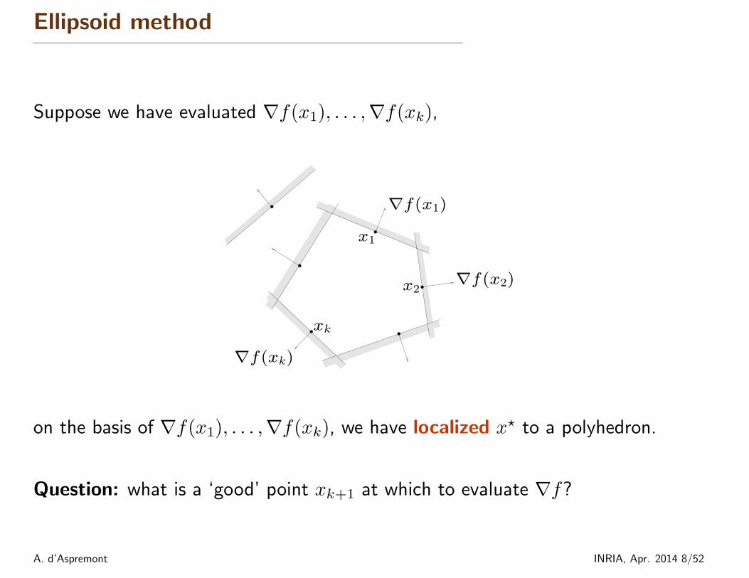
Suppose we have evaluated ∇f(x1), . . . ,∇f(xk),
x1
x2
xk
∇f(x1)
∇f(x2)
∇f(xk)
on the basis of ∇f(x1), . . . ,∇f(xk), we have localized x? to a polyhedron.
Question: what is a ‘good’ point xk+1 at which to evaluate ∇f?
A. d’Aspremont INRIA, Apr. 2014 8/52

Ellipsoid algorithm
Idea: localize x? in an ellipsoid instead of a polyhedron.
E(k)
x(k+1)
∇f(x(k+1))
E(k+1)
Compared to cutting-plane method:
� localization set doesn’t grow more complicated
� easy to compute query point
� but, we add unnecessary points in step 4
A. d’Aspremont INRIA, Apr. 2014 9/52

Ellipsoid Method
Ellipsoid method:
� Simple formula for E(k+1) given E(k)
� vol(E(k+1)) < e−12n vol(E(k))
A. d’Aspremont INRIA, Apr. 2014 10/52

Ellipsoid Method: example
rx(0)
rx(1)r
x(2)
r
x(3)rx(4)
rx(5)
A. d’Aspremont INRIA, Apr. 2014 11/52

Duality
A linear program (LP) is written
minimize cTxsubject to Ax = b
x ≥ 0
where x ≥ 0 means that the coefficients of the vector x are nonnegative.
� Starts with Dantzig’s simplex algorithm in the late 40s.
� First proofs of polynomial complexity by Nemirovskii and Yudin [1979] andKhachiyan [1979] using the ellipsoid method.
� First efficient algorithm with polynomial complexity derived by Karmarkar[1984], using interior point methods.
A. d’Aspremont INRIA, Apr. 2014 12/52

Duality
Duality. The two linear programs
minimize cTx maximize yT bsubject to Ax = b subject to c−ATy ≥ 0
x ≥ 0
have the same optimal values.
� Similar results hold for most convex problems.
� Usually both primal and dual have a natural interpretation.
� Many algorithms solve both problems simultaneously.
A. d’Aspremont INRIA, Apr. 2014 13/52

Support Vector Machines
A. d’Aspremont INRIA, Apr. 2014 14/52
Support Vector Machines
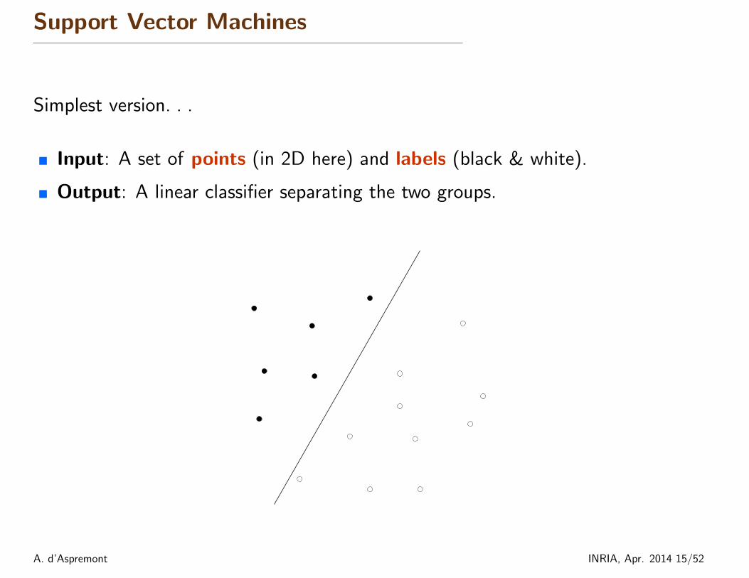
Simplest version. . .
� Input: A set of points (in 2D here) and labels (black & white).
� Output: A linear classifier separating the two groups.
A. d’Aspremont INRIA, Apr. 2014 15/52

Linear Classification
The linear separation problem.
Inputs:
� Data points xj ∈ Rn, j = 1, . . . ,m.
� Binary Labels yj ∈ {−1, 1}, j = 1, . . . ,m.
Problem:
find w ∈ Rn
such that 〈w, xj〉 ≥ 1 for all j such that yj = 1
〈w, xj〉 ≤ −1 for all j such that yj = −1
Output:
� The classifier vector w.
A. d’Aspremont INRIA, Apr. 2014 16/52

Linear Classification
Nonlinear classification.
� The problem:
find w
such that 〈w, xj〉 ≥ 1 for all j such that yj = 1
〈w, xj〉 ≤ −1 for all j such that yj = −1
is linear in the variable w. Solving it amounts to solving a linear program.
� Suppose we want to add quadratic terms in x:
find w
such that 〈w, (xj, x2j)〉 ≥ 1 for all j such that yj = 1
〈w, (xj, x2j)〉 ≤ −1 for all j such that yj = −1
this is still a (larger) linear program in the variable w.
Nonlinear classification is as easy as linear classification.
A. d’Aspremont INRIA, Apr. 2014 17/52

Classification
This trick means that we are not limited to linear classifiers:
Separation by ellipsoid Separation by 4th degree polynomial
Both are equivalent to linear classification. . . just increase the dimension.
A. d’Aspremont INRIA, Apr. 2014 18/52

Classification: margin
Suppose the two sets are not separable. We solve instead
minimize 1Tu+ 1Tv
subject to 〈w, xj〉 ≥ 1− uj for all j such that yj = 1
〈w, xj〉 < −(1− vj) for all j such that yj = −1u � 0, v � 0
Can be interpreted as a heuristic for minimizing the number of misclassified points.
A. d’Aspremont INRIA, Apr. 2014 19/52

Robust linear discrimination
Suppose instead that the two data sets are well separated.
(Euclidean) distance between hyperplanes
H1 = {z | aTz + b = 1}H2 = {z | aTz + b = −1}
is dist(H1,H2) = 2/‖a‖2
to separate two sets of points by maximum margin,
minimize (1/2)‖a‖2subject to aTxi + b ≥ 1, i = 1, . . . , N
aTyi + b ≤ −1, i = 1, . . . ,M
(1)
(after squaring objective) a QP in a, b
A. d’Aspremont INRIA, Apr. 2014 20/52

Classification
In practice. . .
� The data has very high dimension.
� The classifier is highly nonlinear.
� Overfitting is a problem: tradeoff between error and margin.
A. d’Aspremont INRIA, Apr. 2014 21/52

Support Vector Machines: Duality
Given m data points xi ∈ Rn with labels yi ∈ {−1, 1}.
� The maximum margin classification SVM problem can be written
minimize 12‖w‖
22 + C1Tz
subject to yi(wTxi) ≥ 1− zi, i = 1, . . . ,m
z ≥ 0
in the variables w, z ∈ Rn, with parameter C > 0.
� The Lagrangian is written
L(w, z, α) =1
2‖w‖22 + C1Tz +
m∑i=1
αi(1− zi − yiwTxi)
with dual variable α ∈ Rm+ .
A. d’Aspremont INRIA, Apr. 2014 22/52

Support Vector Machines: Duality
� The Lagrangian can be rewritten
L(w, z, α) =1
2
∥∥∥∥∥w −m∑i=1
αiyixi
∥∥∥∥∥2
2
−
∥∥∥∥∥m∑i=1
αiyixi
∥∥∥∥∥2
2
+ (C1− α)Tz + 1Tα
with dual variable α ∈ Rn+.
� Minimizing in (w, z) we form the dual problem
maximize −12 ‖∑m
i=1αiyixi‖2
2+ 1Tα
subject to 0 ≤ α ≤ C
� At the optimum, we must have
w =
m∑i=1
αiyixi and αi = C if zi > 0
(this is the representer theorem).
A. d’Aspremont INRIA, Apr. 2014 23/52

Support Vector Machines: the kernel trick
� If we write X the data matrix with columns xi, the dual can be rewritten
maximize −12α
T diag(y)XTX diag(y)α+ 1Tα
subject to 0 ≤ α ≤ C
� This means that the data only appears in the dual through the gram matrix
K = XTX
which is called the kernel matrix.
� In particular, the original dimension n does not appear in the dual.
� SVM complexity only grows with the number of samples, typically O(m1.5).
A. d’Aspremont INRIA, Apr. 2014 24/52

Support Vector Machines: the kernel trick
Kernels.
� All matrices written K = XTX can be kernel matrices.
� Easy to construct from highly diverse data types.
Examples. . .
� Kernels for voice recognition
0.97 0.975 0.98 0.985 0.99 0.995-1
-0.5
0
0.5
1Voice excerpt
time / sec
Figure 4: Example of vocal waveform during a vowel. We see three cycles of the voice pitch;within each cycle, the waveform looks a lot like an exponentially decaying sinusoid.
3 Linearity
Prior to presenting the central idea of Fourier analysis, there is one more supporting concept to
explore: Linearity. Very roughly, linearity is the idea that scaling the input to a system will result
in scaling the output by the same amount – which was implicit in the choice of using the ratio of
input to output amplitudes in the graph of figure 1 i.e. the ratio of input to output did not depend
on the absolute level of input (at least within reasonable bounds). Linearity is an idealization, but
happily it is widely obeyed in nature, particularly if circumstances are restricted to small deviations
around some stable equilibrium.
In signal processing, we use ‘system’ to mean any process that takes a signal (e.g. a sound
waveform) as input and generates another signal as output. A linear system is one that has the
linearity property, and this constitutes a large class of real- world systems including acoustic envi-
ronments or channels with rigid boundaries, as well as other domains including radio waves and
mechanical systems consisting of rigid connections, ideal springs. and dampers. Of course, most
scenarios of interest also involve some nonlinear components, e.g. the vocal folds that convert
steady air pressure from the lungs into periodic pressure waves in the (largely linear) vocal tract.
Linearity has an important and subtle consequence: superposition. The property of superposi-
tion means that if you know the outputs of a particular system in response to two different inputs,
then the output of the system in response to the sum of the two inputs is simply the sum of the
two outputs. Figure 5 illustrates this. The left columns show inputs, and the right columns show
8
� Kernels for gene sequence alignment
A. d’Aspremont INRIA, Apr. 2014 25/52

Support Vector Machines: the kernel trick
� Kernels for images
200 400 600
100
200
300
400
0
0.1
0.2
1 1.5 2
� Kernels for text classification
Ryanair Q3 profit up 30%, stronger than expected. (From Reuters.)DUBLIN, Feb 5 (Reuters) - Ryanair (RYA.I: Quote, Profile , Research)posted a 30 pct jump in third-quarter net profit on Monday, confoundinganalyst expectations for a fall, and ramped up its full-year profit goalwhile predicting big fuel-cost savings for the following year (. . . ).
profit loss up down jump fall below expectations ramped up
3 0 2 0 1 1 0 1 1
A. d’Aspremont INRIA, Apr. 2014 26/52

Compressed Sensing
A. d’Aspremont INRIA, Apr. 2014 27/52
Compressed Sensing
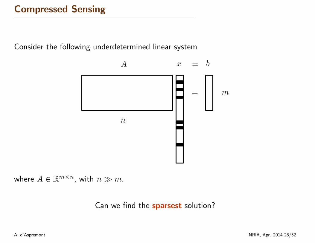
Consider the following underdetermined linear system
n
m
A x =
=
b
where A ∈ Rm×n, with n� m.
Can we find the sparsest solution?
A. d’Aspremont INRIA, Apr. 2014 28/52
Compressed Sensing
� Signal processing: We make a few measurements of a high dimensionalsignal, which admits a sparse representation in a well chosen basis (e.g.Fourier, wavelet). Can we reconstruct the signal exactly?
� Coding: Suppose we transmit a message which is corrupted by a few errors.How many errors does it take to start losing the signal?
� Statistics: Variable selection in regression (LASSO, etc).
A. d’Aspremont INRIA, Apr. 2014 29/52

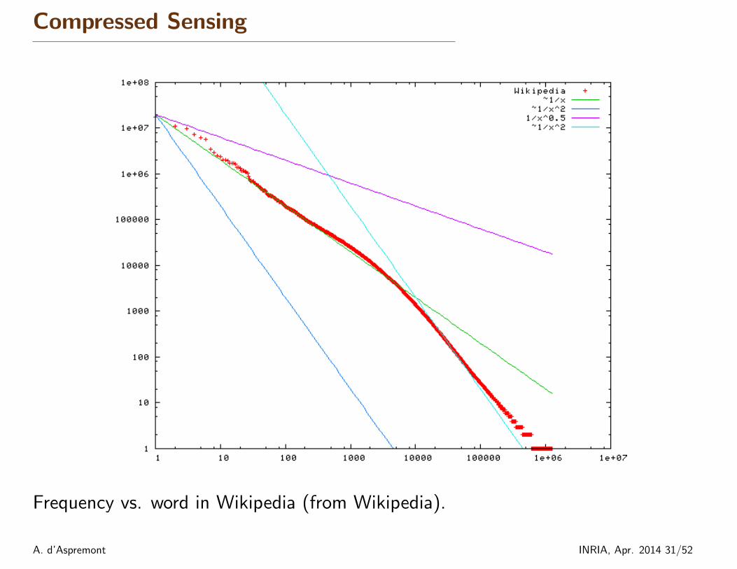
Compressed Sensing
Why sparsity?
� Sparsity is a proxy for power laws. Most results stated here on sparse vectorsapply to vectors with a power law decay in coefficient magnitude.
� Power laws appear everywhere. . .
◦ Zipf law: word frequencies in natural language follow a power law.
◦ Ranking: pagerank coefficients follow a power law.
◦ Signal processing: 1/f signals
◦ Social networks: node degrees follow a power law.
◦ Earthquakes: Gutenberg-Richter power laws
◦ River systems, cities, net worth, etc.
A. d’Aspremont INRIA, Apr. 2014 30/52
Compressed Sensing
Frequency vs. word in Wikipedia (from Wikipedia).
A. d’Aspremont INRIA, Apr. 2014 31/52

Compressed Sensing
Frequency vs. magnitude for earthquakes worldwide. [Christensen et al., 2002]
A. d’Aspremont INRIA, Apr. 2014 32/52

Compressed Sensing
10 Internet Mathematics
!"#$%
$&$$$!
$&$$!
$&$!
$&!
!"#$' !"#$% $&$$$! $&$$!
()*+,-./0.(01"),-+"2
3*4")*/5
3)678090:"#!;<7==>&!
Figure 3. Log-log plot of the PageRank distribution of the Brown domain(*.brown.edu). A vast majority of the pages (except those with very low Page-Rank) follow a power law with exponent close to 2.1. The plot almost flattensout for pages with very low PageRank.
!"#$'
!"#$%
$&$$$!
$&$$!
$&$!
$&!
!
!"#$? !"#$' !"#$% $&$$$! $&$$!
()*+,-./0.(01"),-+"2
3*4")*/5
3)678090@"#!%<7==>&!
Figure 4. Log-log plot of the PageRank distribution of the WT10g corpus. Theslope is close to 2.1. Note that the plot looks much sharper than the correspondingplot for the Brown web. Also, the tapering at the top is much less pronounced.Pages vs. Pagerank on web sample. [Pandurangan et al., 2006]
A. d’Aspremont INRIA, Apr. 2014 33/52

Compressed Sensing14 The structure and function of complex networks
1 10 100
10-4
10-2
100
1 10 100 1000
10-4
10-2
100
100
102
104
10610
-8
10-6
10-4
10-2
100
1 10 100 100010
-4
10-3
10-2
10-1
100
0 10 20
10-3
10-2
10-1
100
1 10
10-3
10-2
10-1
100
(a) collaborations
in mathematics (b) citations (c) World Wide Web
(d) Internet (e) power grid(f) protein
interactions
FIG. 6 Cumulative degree distributions for six di!erent networks. The horizontal axis for each panel is vertex degree k (or in-degree for the citation and Web networks, which are directed) and the vertical axis is the cumulative probability distribution ofdegrees, i.e., the fraction of vertices that have degree greater than or equal to k. The networks shown are: (a) the collaborationnetwork of mathematicians [182]; (b) citations between 1981 and 1997 to all papers cataloged by the Institute for ScientificInformation [351]; (c) a 300 million vertex subset of the World Wide Web, circa 1999 [74]; (d) the Internet at the level ofautonomous systems, April 1999 [86]; (e) the power grid of the western United States [416]; (f) the interaction network ofproteins in the metabolism of the yeast S. Cerevisiae [212]. Of these networks, three of them, (c), (d) and (f), appear to havepower-law degree distributions, as indicated by their approximately straight-line forms on the doubly logarithmic scales, andone (b) has a power-law tail but deviates markedly from power-law behavior for small degree. Network (e) has an exponentialdegree distribution (note the log-linear scales used in this panel) and network (a) appears to have a truncated power-law degreedistribution of some type, or possibly two separate power-law regimes with di!erent exponents.
degree distribution overall but unimodal distributionswithin domains [338].
2. Maximum degree
The maximum degree kmax of a vertex in a networkwill in general depend on the size of the network. Forsome calculations on networks the value of this maxi-mum degree matters (see, for example, Sec. VIII.C.2).In work on scale-free networks, Aiello et al. [8] assumedthat the maximum degree was approximately the valueabove which there is less than one vertex of that degree inthe graph on average, i.e., the point where npk = 1. Thismeans, for instance, that kmax ! n1/! for the power-lawdegree distribution pk ! k!!. This assumption howevercan give misleading results; in many cases there will bevertices in the network with significantly higher degreethan this, as discussed by Adamic et al. [6].
Given a particular degree distribution (and assumingall degrees to be sampled independently from it, whichmay not be true for networks in the real world), the prob-ability of there being exactly m vertices of degree k and
no vertices of higher degree is!nm
"
pmk (1"Pk)n!m, where
Pk is the cumulative probability distribution, Eq. (7).Hence the probability hk that the highest degree on thegraph is k is
hk =n
#
m=1
$
n
m
%
pmk (1 " Pk)n!m
= (pk + 1 " Pk)n " (1 " Pk)n, (10)
and the expected value of the highest degree is kmax =&
k khk.For both small and large values of k, hk tends to zero,
and the sum over k is dominated by the terms close to themaximum. Thus, in most cases, a good approximationto the expected value of the maximum degree is givenby the modal value. Di!erentiating and observing thatdPk/dk = pk, we find that the maximum of hk occurswhen$
dpk
dk" pk
%
(pk +1"Pk)n!1 + pk(1"Pk)n!1 = 0, (11)
or kmax is a solution of
dpk
dk# "np2
k, (12)
Cumulative degree distribution in networks. [Newman, 2003]
A. d’Aspremont INRIA, Apr. 2014 34/52
Compressed Sensing
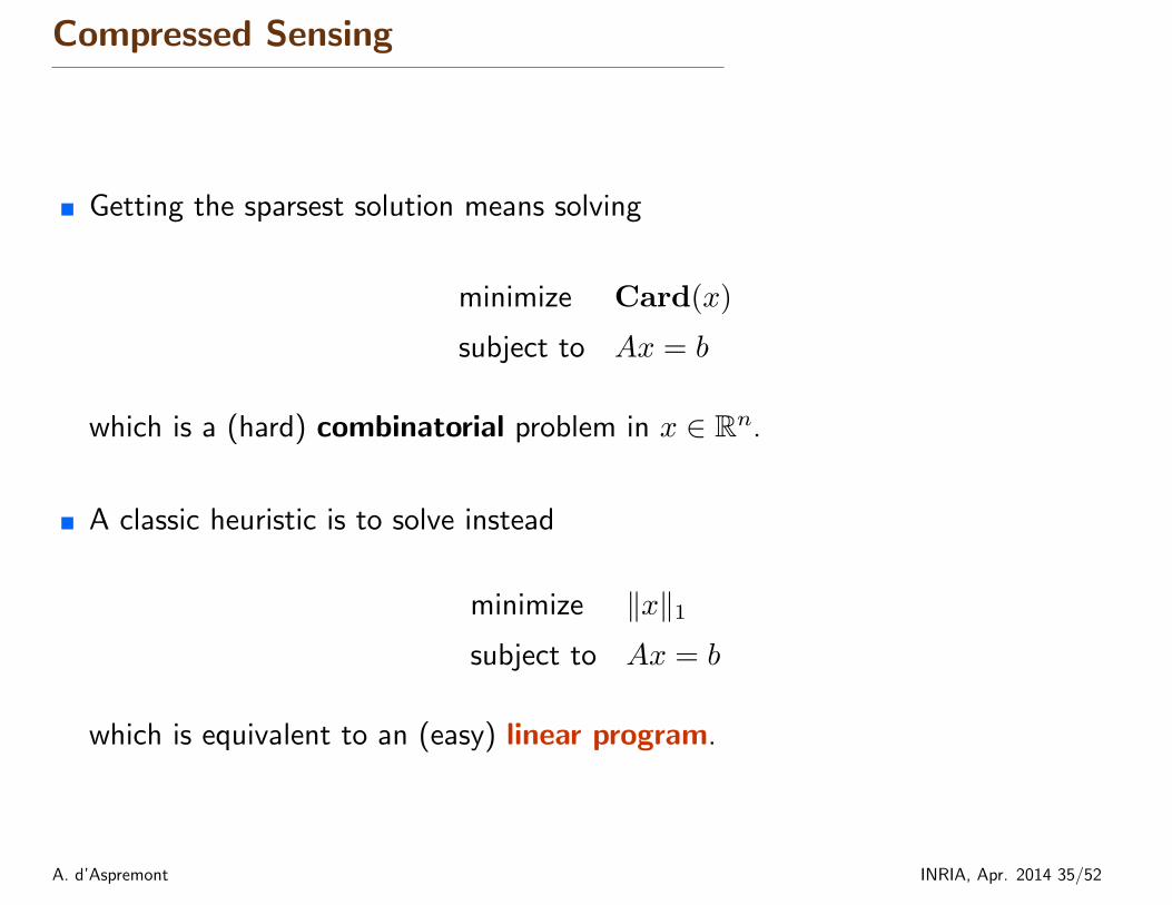
� Getting the sparsest solution means solving
minimize Card(x)
subject to Ax = b
which is a (hard) combinatorial problem in x ∈ Rn.
� A classic heuristic is to solve instead
minimize ‖x‖1subject to Ax = b
which is equivalent to an (easy) linear program.
A. d’Aspremont INRIA, Apr. 2014 35/52

Compressed Sensing
Example: we fix A and draw many sparse signals e. Plot the probability ofperfectly recovering e by solving
minimize ‖x‖1subject to Ax = Ae
in x ∈ Rn, with n = 50 and m = 30.
0 10 20 30 40 500
0.2
0.4
0.6
0.8
1
Cardinality of e
Prob.ofrecoveringe
A. d’Aspremont INRIA, Apr. 2014 36/52

Compressed Sensing
� For some matrices A, when the solution e is sparse enough, the solution of thelinear program problem is also the sparsest solution to Ax = Ae. [Donohoand Tanner, 2005, Candes and Tao, 2005]
� Let k = Card(e), this happens even when k = O(m) asymptotically, which isprovably optimal.
0 0.2 0.4 0.6 0.8 10
0.2
0.4
0.6
0.8
1
Cardinality
k/m
Shape m/n
A. d’Aspremont INRIA, Apr. 2014 37/52

Semidefinite Programming
A. d’Aspremont INRIA, Apr. 2014 38/52

Semidefinite Programming
A linear program (LP) is written
minimize cTx
subject to Ax = b
x ≥ 0
where x ≥ 0 means that the coefficients of the vector x are nonnegative.
A. d’Aspremont INRIA, Apr. 2014 39/52

Semidefinite Programming
A semidefinite program (SDP) is written
minimize Tr(CX)
subject to Tr(AiX) = bi, i = 1, . . . ,m
X � 0
where X � 0 means that the matrix variable X ∈ Sn is positive semidefinite.
� Nesterov and Nemirovskii [1994] showed that the interior point algorithmsused for linear programs could be extended to semidefinite programs.
� Key result: self-concordance analysis of Newton’s method (affine invariantsmoothness bounds on the Hessian).
A. d’Aspremont INRIA, Apr. 2014 40/52
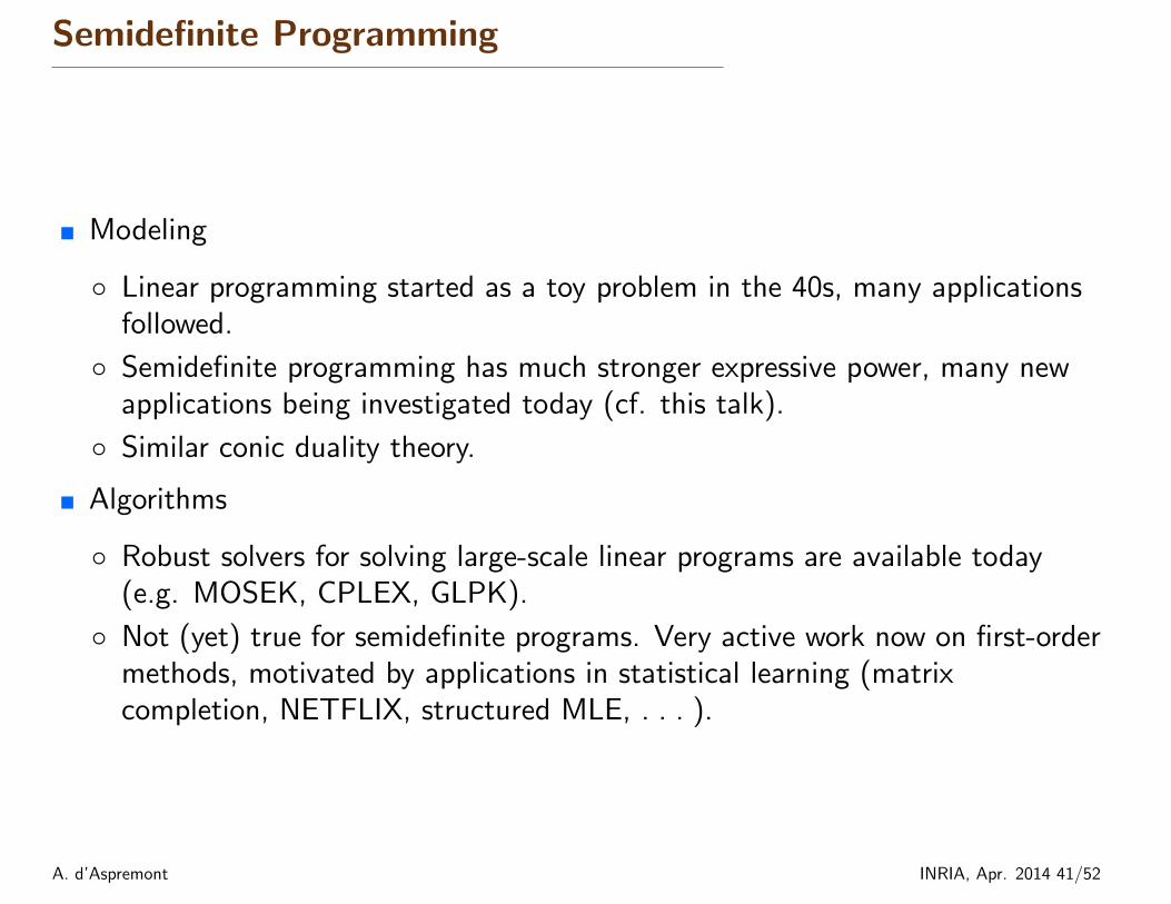
Semidefinite Programming
� Modeling
◦ Linear programming started as a toy problem in the 40s, many applicationsfollowed.
◦ Semidefinite programming has much stronger expressive power, many newapplications being investigated today (cf. this talk).
◦ Similar conic duality theory.
� Algorithms
◦ Robust solvers for solving large-scale linear programs are available today(e.g. MOSEK, CPLEX, GLPK).
◦ Not (yet) true for semidefinite programs. Very active work now on first-ordermethods, motivated by applications in statistical learning (matrixcompletion, NETFLIX, structured MLE, . . . ).
A. d’Aspremont INRIA, Apr. 2014 41/52

The NETFLIX challenge
A. d’Aspremont INRIA, Apr. 2014 42/52

NETFLIX
� Video On Demand and DVD by mail service in the United States, Canada,Latin America, the Caribbean, United Kingdom, Ireland, Sweden, Denmark,Norway, Finland.
� About 25 million users and 60,000 films.
� Unlimited streaming, DVD mailing, cheaper than CANAL+ :)
� Online movie recommendation engine.
A. d’Aspremont INRIA, Apr. 2014 43/52

Collaborative prediction
� Users assign ratings to a certain number of movies:
Use
rs
Movies
� Objective: make recommendations for other movies. . .
A. d’Aspremont INRIA, Apr. 2014 44/52

NETFLIX25/11/12 21:31Netflix
Page 1 of 10http://movies.netflix.com/WiHome
Your taste preferencescreated this row.
Visually-strikingAction & Adventure.
As well as your interest in…
Top 10 for alexandre
Popular on Netflix
Visually-striking Action & Adventure
Exciting Movies
InstantQueue
DVDsalexandre d'Aspr… Your Account Help
Movies, TV shows, actors, directors, genres Just for
Kids Taste
Profile
A. d’Aspremont INRIA, Apr. 2014 45/52
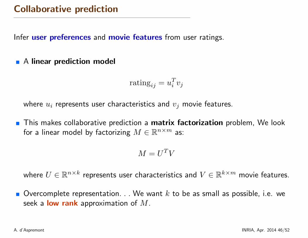
Collaborative prediction
Infer user preferences and movie features from user ratings.
� A linear prediction model
ratingij = uTi vj
where ui represents user characteristics and vj movie features.
� This makes collaborative prediction a matrix factorization problem, We lookfor a linear model by factorizing M ∈ Rn×m as:
M = UTV
where U ∈ Rn×k represents user characteristics and V ∈ Rk×m movie features.
� Overcomplete representation. . . We want k to be as small as possible, i.e. weseek a low rank approximation of M .
A. d’Aspremont INRIA, Apr. 2014 46/52

Collaborative prediction
� We would like to solve
minimize Rank(X) + c∑
(i,j)∈S
max(0, 1−XijMij)
non-convex and numerically hard. . .
� Relaxation result in Fazel et al. [2001]: replace Rank(X) by its convexenvelope on the spectahedron to solve:
minimize ‖X‖∗ + c∑
(i,j)∈S
max(0, 1−XijMij)
where ‖X‖∗ is the nuclear norm, i.e. sum of the singular values of X.
� This is a convex semidefinite program in X.
A. d’Aspremont INRIA, Apr. 2014 47/52

Collaborative prediction
NETFLIX challenge.
� NETFLIX offered $1 million to the team who could improve the quality of itsratings by 10%, and $50.000 to the first team to improve them by 1%.
� It took two weeks to beat the 1% mark, and three years to reach 10%.
� Very large number of scientists, students, postdocs, etc. working on this.
� The story could end here. But all this work had surprising outcomes. . .
A. d’Aspremont INRIA, Apr. 2014 48/52

Phase Recovery
Molecular imaging
Origin: X-ray crystallography
Knowledge of phase crucial to build electron density map
Initial success in certain cases by using very specific prior knowledge: NobelPrize for Hauptman and Karle (1985)
Still important today: e.g. macromolecular crystallography for drug design
(from [Candes et al., 2011])
� CCD sensors only record the magnitude of diffracted rays, and loose the phase
� Fraunhofer diffraction: phase is required to invert the 2D Fourier transform
A. d’Aspremont INRIA, Apr. 2014 49/52
Phase Recovery
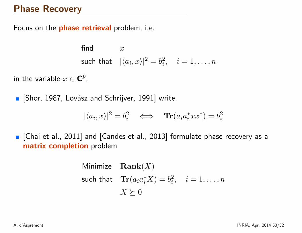
Focus on the phase retrieval problem, i.e.
find x
such that |〈ai, x〉|2 = b2i , i = 1, . . . , n
in the variable x ∈ Cp.
� [Shor, 1987, Lovasz and Schrijver, 1991] write
|〈ai, x〉|2 = b2i ⇐⇒ Tr(aia∗ixx∗) = b2i
� [Chai et al., 2011] and [Candes et al., 2013] formulate phase recovery as amatrix completion problem
Minimize Rank(X)
such that Tr(aia∗iX) = b2i , i = 1, . . . , n
X � 0
A. d’Aspremont INRIA, Apr. 2014 50/52

Phase Recovery
[Recht et al., 2007, Candes and Recht, 2008, Candes and Tao, 2010] show thatunder certain conditions on A and x0, it suffices to solve
Minimize Tr(X)
such that Tr(aia∗iX) = b2i , i = 1, . . . , n
X � 0
which is a (convex) semidefinite program in X ∈ Hp.
� Solving the convex semidefinite program yields a solution to the combinatorial,hard reconstruction problem.
� Apply results from collaborative filtering (NETFLIX) to molecular imaging.
A. d’Aspremont INRIA, Apr. 2014 51/52

Phase Recovery
Merci!
A. d’Aspremont INRIA, Apr. 2014 52/52

*
References
E. J. Candes and T. Tao. Decoding by linear programming. IEEE Transactions on Information Theory, 51(12):4203–4215, 2005.
E. J. Candes, T. Strohmer, and V. Voroninski. Phaselift : exact and stable signal recovery from magnitude measurements via convexprogramming. To appear in Communications in Pure and Applied Mathematics, 66(8):1241–1274, 2013.
E.J. Candes and B. Recht. Exact matrix completion via convex optimization. preprint, 2008.
E.J. Candes and T. Tao. The power of convex relaxation: Near-optimal matrix completion. Information Theory, IEEE Transactions on, 56(5):2053–2080, 2010.
E.J. Candes, Y. Eldar, T. Strohmer, and V. Voroninski. Phase retrieval via matrix completion. Arxiv preprint arXiv:1109.0573, 2011.
A. Chai, M. Moscoso, and G. Papanicolaou. Array imaging using intensity-only measurements. Inverse Problems, 27:015005, 2011.
K. Christensen, L. Danon, T. Scanlon, and P. Bak. Unified scaling law for earthquakes, 2002.
D. L. Donoho and J. Tanner. Sparse nonnegative solutions of underdetermined linear equations by linear programming. Proc. of the NationalAcademy of Sciences, 102(27):9446–9451, 2005.
M. Fazel, H. Hindi, and S. Boyd. A rank minimization heuristic with application to minimum order system approximation. ProceedingsAmerican Control Conference, 6:4734–4739, 2001.
N. K. Karmarkar. A new polynomial-time algorithm for linear programming. Combinatorica, 4:373–395, 1984.
L. G. Khachiyan. A polynomial algorithm in linear programming (in Russian). Doklady Akademiia Nauk SSSR, 224:1093–1096, 1979.
L. Lovasz and A. Schrijver. Cones of matrices and set-functions and 0-1 optimization. SIAM Journal on Optimization, 1(2):166–190, 1991.
A. Nemirovskii and D. Yudin. Problem complexity and method efficiency in optimization. Nauka (published in English by John Wiley,Chichester, 1983), 1979.
Y. Nesterov and A. Nemirovskii. Interior-point polynomial algorithms in convex programming. Society for Industrial and AppliedMathematics, Philadelphia, 1994.
MEJ Newman. The structure and function of complex networks. Arxiv preprint cond-mat/0303516, 2003.
G. Pandurangan, P. Raghavan, and E. Upfal. Using pagerank to characterize web structure. Internet Mathematics, 3(1):1–20, 2006.
B. Recht, M. Fazel, and P.A. Parrilo. Guaranteed Minimum-Rank Solutions of Linear Matrix Equations via Nuclear Norm Minimization. Arxivpreprint arXiv:0706.4138, 2007.
N.Z. Shor. Quadratic optimization problems. Soviet Journal of Computer and Systems Sciences, 25:1–11, 1987.
J. Sun, S. Boyd, L. Xiao, and P. Diaconis. The fastest mixing Markov process on a graph and a connection to a maximum variance unfoldingproblem. SIAM Review, 48(4):681–699, 2006.
A. d’Aspremont INRIA, Apr. 2014 53/52

K.Q. Weinberger and L.K. Saul. Unsupervised Learning of Image Manifolds by Semidefinite Programming. International Journal of ComputerVision, 70(1):77–90, 2006.
A. d’Aspremont INRIA, Apr. 2014 54/52