Albert Tarantola - IPGP
305
Transcript of Albert Tarantola - IPGP


Albert Tarantola∗Université de Paris, Institut de Physique du Globe4, place Jussieu; 75005 Paris; France
E-mail: [email protected]
Mapping of Probabilities
Theory for the Interpretation of
Uncertain Physical Measurements
April 10, 2007
Submitted to Cambridge University Press∗ © A. Tarantola, 2006.

II

III
To Kike & Vittorio.

IV

PrefaceIn this book, I attempt to reach two goals. The first is purely mathemat-
ical: to clarify some of the basic concepts of probability theory. The secondgoal is physical: to clarify the methods to be used when handling the infor-mation brought by measurements, in order to understand how accurate arethe inferences they allow.
Probability theory is solidly based on Kolmogorov axioms, but the basicinference tool provided by Kolmogorov’s theory is the definition of condi-tional probability. While some simple problems can be solved though thisnotion of conditional probability, more elaborate problems, in particular,most of the inference problems that use inaccurate observations require amore advanced probability theory.
When considering sets, there are some well known notions, for instance,the intersection of two sets, or, when a mapping is considered between twosets, the notion of image of a set, or of reciprocal image of a set. I developin this book the theory that generalizes these notions when, instead of sets,we consider probabilities: what is the intersection of two probabilities, theimage of a probability, and the reciprocal image of a probability? Attachedto these definitions, a theorem is found that suggests an alternative for set-ting some inference problems (like, for instance, the so-called “inverse prob-lems”), that, I suggest, are not to be seen as problems of conditional proba-bility.
The discrepancy between the two approaches is not only conceptual. Inthe case where manifolds are involved (and this is every time a physicistsconsiders a quantity taking real values), the notion of probability densityhas to be introduced, and it is well known that conditional probability densi-ties are problematic (from where some well-known paradoxes, like the Borelparadox). When using the theory proposed in this book, one arrives to re-sults that are quantitatively different from those obtained with the theorygenerally used.
In chapter one. . . In chapter two. . . In chapter three. . . Finally, in chapterfour. . .
I am very indebted to my colleagues (Bartolomé Coll, Georges Jobert,Klaus Mosegaard, Miguel Bosch, and Guillaume Évrard) for illuminatingdiscussions.
Paris, April 10, 2007Albert Tarantola


Contents
1 Sets . . . . . . . . . . . . . . . . . . . . . . . . . . . . . . . . . . . . . . . . . . . . . . . . . . . . . . . . . . 11.1 Sets . . . . . . . . . . . . . . . . . . . . . . . . . . . . . . . . . . . . . . . . . . . . . . . . . . . . . . 11.2 Mappings . . . . . . . . . . . . . . . . . . . . . . . . . . . . . . . . . . . . . . . . . . . . . . . . 61.3 Assimilation of Observations . . . . . . . . . . . . . . . . . . . . . . . . . . . . . . 10
1.3.1 Method . . . . . . . . . . . . . . . . . . . . . . . . . . . . . . . . . . . . . . . . . . . . 101.3.2 Example . . . . . . . . . . . . . . . . . . . . . . . . . . . . . . . . . . . . . . . . . . . 11
2 Probabilities . . . . . . . . . . . . . . . . . . . . . . . . . . . . . . . . . . . . . . . . . . . . . . . . . . 152.1 Basic Definitions . . . . . . . . . . . . . . . . . . . . . . . . . . . . . . . . . . . . . . . . . . 152.2 Intersection of Probabilities . . . . . . . . . . . . . . . . . . . . . . . . . . . . . . . . 232.3 Image of a Probability . . . . . . . . . . . . . . . . . . . . . . . . . . . . . . . . . . . . . 272.4 Reciprocal Image of a Probability . . . . . . . . . . . . . . . . . . . . . . . . . . 312.5 The Bayes-Popper Problem . . . . . . . . . . . . . . . . . . . . . . . . . . . . . . . . 33
2.5.1 Method . . . . . . . . . . . . . . . . . . . . . . . . . . . . . . . . . . . . . . . . . . . . 332.5.2 Example . . . . . . . . . . . . . . . . . . . . . . . . . . . . . . . . . . . . . . . . . . . 392.5.3 Example . . . . . . . . . . . . . . . . . . . . . . . . . . . . . . . . . . . . . . . . . . . 40
3 Physical Quantities, Manifolds, and Physical Measurements . . . . 453.1 Physical Quantities: the Intrinsic Point of View . . . . . . . . . . . . . . 463.2 Expressing the Results of Measurements . . . . . . . . . . . . . . . . . . . . 513.3 Examples . . . . . . . . . . . . . . . . . . . . . . . . . . . . . . . . . . . . . . . . . . . . . . . . 54
4 Examples . . . . . . . . . . . . . . . . . . . . . . . . . . . . . . . . . . . . . . . . . . . . . . . . . . . . . 594.1 Finding the Homogeneous Probability Density . . . . . . . . . . . . . . 60
4.1.1 Homogeneous Probability for Elastic Parameters . . . . . 604.2 Problems Solved Using a Change of Variables . . . . . . . . . . . . . . . 65
4.2.1 Measuring a One-Dimensional Strain (I) . . . . . . . . . . . . . . 654.2.2 Measuring a One-Dimensional Strain (II) . . . . . . . . . . . . . 674.2.3 Measure of Poisson’s Ratio . . . . . . . . . . . . . . . . . . . . . . . . . . 704.2.4 Mass Calibration . . . . . . . . . . . . . . . . . . . . . . . . . . . . . . . . . . . 81
4.3 Problems Solved Using the Image of a Probability . . . . . . . . . . . 834.3.1 Free-Fall of an Object . . . . . . . . . . . . . . . . . . . . . . . . . . . . . . . 83
4.4 Problems Solved using the Popper-Bayes Paradigm . . . . . . . . . 864.4.1 Model of a Volcano . . . . . . . . . . . . . . . . . . . . . . . . . . . . . . . . . 864.4.2 Earthquake Location . . . . . . . . . . . . . . . . . . . . . . . . . . . . . . . . 86

VIII Contents
5 Appendix: Manifolds (provisional) . . . . . . . . . . . . . . . . . . . . . . . . . . . . 935.1 Manifolds and Coordinates . . . . . . . . . . . . . . . . . . . . . . . . . . . . . . . . 93
5.1.1 Linear Spaces . . . . . . . . . . . . . . . . . . . . . . . . . . . . . . . . . . . . . . 945.1.2 Manifolds . . . . . . . . . . . . . . . . . . . . . . . . . . . . . . . . . . . . . . . . . 955.1.3 Changing Coordinates . . . . . . . . . . . . . . . . . . . . . . . . . . . . . . 965.1.4 Tensors, Capacities, and Densities . . . . . . . . . . . . . . . . . . . 975.1.5 Kronecker Tensors (I) . . . . . . . . . . . . . . . . . . . . . . . . . . . . . . . 995.1.6 Orientation of a Manifold . . . . . . . . . . . . . . . . . . . . . . . . . . . 1005.1.7 Totally Antisymmetric Tensors . . . . . . . . . . . . . . . . . . . . . . 1015.1.8 Levi-Civita Capacity and Density . . . . . . . . . . . . . . . . . . . . 1015.1.9 Determinants . . . . . . . . . . . . . . . . . . . . . . . . . . . . . . . . . . . . . . 1025.1.10 Dual Tensors and Exterior Product of Vectors . . . . . . . . . 1035.1.11 Capacity Element (trying a new text) . . . . . . . . . . . . . . . . . 1045.1.12 Capacity Element (old text) . . . . . . . . . . . . . . . . . . . . . . . . . 1055.1.13 Integral (new text) . . . . . . . . . . . . . . . . . . . . . . . . . . . . . . . . . . 1075.1.14 Integral (old text) . . . . . . . . . . . . . . . . . . . . . . . . . . . . . . . . . . . 1105.1.15 Capacity Element and Change of Coordinates . . . . . . . . 111
5.2 Volume . . . . . . . . . . . . . . . . . . . . . . . . . . . . . . . . . . . . . . . . . . . . . . . . . . 1125.2.1 Metric . . . . . . . . . . . . . . . . . . . . . . . . . . . . . . . . . . . . . . . . . . . . . 1125.2.2 Bijection Between Forms and Vectors . . . . . . . . . . . . . . . . 1135.2.3 Kronecker Tensor (II) . . . . . . . . . . . . . . . . . . . . . . . . . . . . . . . 1145.2.4 Fundamental Density . . . . . . . . . . . . . . . . . . . . . . . . . . . . . . . 1145.2.5 Bijection Between Capacities, Tensors, and Densities . . 1155.2.6 Levi-Civita Tensor . . . . . . . . . . . . . . . . . . . . . . . . . . . . . . . . . . 1155.2.7 Volume Element . . . . . . . . . . . . . . . . . . . . . . . . . . . . . . . . . . . . 1165.2.8 Volume Element and Change of Variables . . . . . . . . . . . . 1175.2.9 Volume of a Domain . . . . . . . . . . . . . . . . . . . . . . . . . . . . . . . . 1185.2.10 Example: Mass Density and Volumetric Mass . . . . . . . . . 119
5.3 Mappings . . . . . . . . . . . . . . . . . . . . . . . . . . . . . . . . . . . . . . . . . . . . . . . . 1215.3.1 Image of the Volume Element . . . . . . . . . . . . . . . . . . . . . . . 1215.3.2 Reciprocal Image of the Volume Element . . . . . . . . . . . . . 122
5.4 Appendices for Manifolds (check) . . . . . . . . . . . . . . . . . . . . . . . . . . 1225.4.1 Capacity Element and Change of Coordinates . . . . . . . . 1225.4.2 Conditional Volume . . . . . . . . . . . . . . . . . . . . . . . . . . . . . . . . 123
6 Appendix: Marginal and Conditional Probabilities (veryprovisional) . . . . . . . . . . . . . . . . . . . . . . . . . . . . . . . . . . . . . . . . . . . . . . . . . . . 1276.1 Conditional Probability Function . . . . . . . . . . . . . . . . . . . . . . . . . . . 127
6.1.1 Conditional Probability (provisional text I) . . . . . . . . . . . 1276.1.2 Conditional Probability (provisional text II) . . . . . . . . . . 1286.1.3 Conditional Probability (provisional text III) . . . . . . . . . . 1306.1.4 Conditional Probability (provisional text IV) . . . . . . . . . . 1316.1.5 Conditional Probability (provisional text V) . . . . . . . . . . 1366.1.6 Conditional Probability (provisional text VI) . . . . . . . . . . 1376.1.7 Conditional Probability (provisional text VII) . . . . . . . . . 142

Contents IX
6.1.8 Conditional Probability (provisional text VIII) . . . . . . . . 1446.2 Marginal Probability Function . . . . . . . . . . . . . . . . . . . . . . . . . . . . . 147
6.2.1 Marginal Probability (provisional text I) . . . . . . . . . . . . . . 1476.2.2 Marginal Probability (provisional text II) . . . . . . . . . . . . . 1496.2.3 Marginal Probability (provisional text III) . . . . . . . . . . . . 150
6.3 Independence . . . . . . . . . . . . . . . . . . . . . . . . . . . . . . . . . . . . . . . . . . . . 1526.4 Marginals of the Conditional . . . . . . . . . . . . . . . . . . . . . . . . . . . . . . 153
6.4.1 Discrete Probabilities . . . . . . . . . . . . . . . . . . . . . . . . . . . . . . . 1536.4.2 Manifolds . . . . . . . . . . . . . . . . . . . . . . . . . . . . . . . . . . . . . . . . . 1536.4.3 Comparison Between Bayes-Popper and Marginal of
the Conditional . . . . . . . . . . . . . . . . . . . . . . . . . . . . . . . . . . . . 1546.4.4 Marginal of a Conditional Probability . . . . . . . . . . . . . . . . 1556.4.5 Demonstration: marginals of the conditional . . . . . . . . . . 156
6.5 The Borel ‘Paradox’ . . . . . . . . . . . . . . . . . . . . . . . . . . . . . . . . . . . . . . . 1586.6 Problems Solved Using Conditional Probabilities . . . . . . . . . . . . 162
6.6.1 Example: Artificial Illustration . . . . . . . . . . . . . . . . . . . . . . . 1626.6.2 Example: Chemical Concentrations . . . . . . . . . . . . . . . . . . 1626.6.3 Example: Adjusting a Measurement to a Theory . . . . . . 164
7 Appendix: Sampling a Probability Function (very provisional) . . 1677.1 Sampling a Probability . . . . . . . . . . . . . . . . . . . . . . . . . . . . . . . . . . . . 167
7.1.1 Sample Points (I) . . . . . . . . . . . . . . . . . . . . . . . . . . . . . . . . . . . 1677.1.2 Sample Points (II) . . . . . . . . . . . . . . . . . . . . . . . . . . . . . . . . . . 1687.1.3 Introduction . . . . . . . . . . . . . . . . . . . . . . . . . . . . . . . . . . . . . . . 1687.1.4 Notion of Sample . . . . . . . . . . . . . . . . . . . . . . . . . . . . . . . . . . . 1717.1.5 Inversion Method . . . . . . . . . . . . . . . . . . . . . . . . . . . . . . . . . . 1717.1.6 Rejection Method . . . . . . . . . . . . . . . . . . . . . . . . . . . . . . . . . . . 1717.1.7 Sequential Realization . . . . . . . . . . . . . . . . . . . . . . . . . . . . . . 172
7.2 Monte Carlo (Sampling) Methods . . . . . . . . . . . . . . . . . . . . . . . . . . 1737.2.1 Random Walks and the Metropolis Rule . . . . . . . . . . . . . . 1737.2.2 Modification of Random Walks . . . . . . . . . . . . . . . . . . . . . . 1737.2.3 The Metropolis Rule . . . . . . . . . . . . . . . . . . . . . . . . . . . . . . . . 1747.2.4 The Cascaded Metropolis Rule . . . . . . . . . . . . . . . . . . . . . . 1757.2.5 Initiating a Random Walk . . . . . . . . . . . . . . . . . . . . . . . . . . . 1757.2.6 Choosing Random Directions and Step Lengths . . . . . . . 176
7.3 Random Points on the Surface of the Sphere . . . . . . . . . . . . . . . . 177
8 Appendix: Demonstrations . . . . . . . . . . . . . . . . . . . . . . . . . . . . . . . . . . . . 1798.1 Compatibility Property . . . . . . . . . . . . . . . . . . . . . . . . . . . . . . . . . . . . 179
8.1.1 Proof of the Compatibility Property (Sets) . . . . . . . . . . . . 1798.1.2 Proof of the Compatibility Property (Probabilities) . . . . 179
8.2 Image of a Probability Density . . . . . . . . . . . . . . . . . . . . . . . . . . . . . 1838.2.1 New Example . . . . . . . . . . . . . . . . . . . . . . . . . . . . . . . . . . . . . . 1838.2.2 Old Text . . . . . . . . . . . . . . . . . . . . . . . . . . . . . . . . . . . . . . . . . . . 186
X Contents
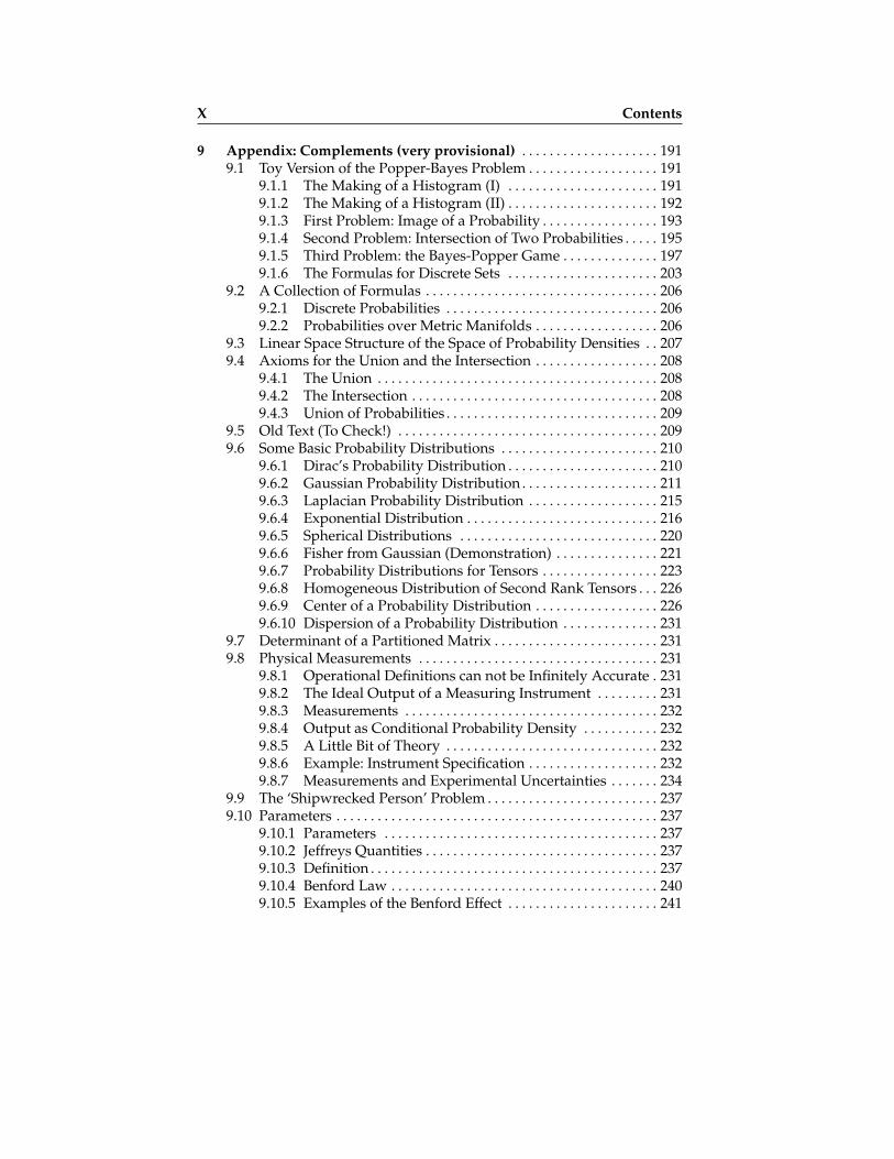
9 Appendix: Complements (very provisional) . . . . . . . . . . . . . . . . . . . . 1919.1 Toy Version of the Popper-Bayes Problem . . . . . . . . . . . . . . . . . . . 191
9.1.1 The Making of a Histogram (I) . . . . . . . . . . . . . . . . . . . . . . 1919.1.2 The Making of a Histogram (II) . . . . . . . . . . . . . . . . . . . . . . 1929.1.3 First Problem: Image of a Probability . . . . . . . . . . . . . . . . . 1939.1.4 Second Problem: Intersection of Two Probabilities . . . . . 1959.1.5 Third Problem: the Bayes-Popper Game . . . . . . . . . . . . . . 1979.1.6 The Formulas for Discrete Sets . . . . . . . . . . . . . . . . . . . . . . 203
9.2 A Collection of Formulas . . . . . . . . . . . . . . . . . . . . . . . . . . . . . . . . . . 2069.2.1 Discrete Probabilities . . . . . . . . . . . . . . . . . . . . . . . . . . . . . . . 2069.2.2 Probabilities over Metric Manifolds . . . . . . . . . . . . . . . . . . 206
9.3 Linear Space Structure of the Space of Probability Densities . . 2079.4 Axioms for the Union and the Intersection . . . . . . . . . . . . . . . . . . 208
9.4.1 The Union . . . . . . . . . . . . . . . . . . . . . . . . . . . . . . . . . . . . . . . . . 2089.4.2 The Intersection . . . . . . . . . . . . . . . . . . . . . . . . . . . . . . . . . . . . 2089.4.3 Union of Probabilities . . . . . . . . . . . . . . . . . . . . . . . . . . . . . . . 209
9.5 Old Text (To Check!) . . . . . . . . . . . . . . . . . . . . . . . . . . . . . . . . . . . . . . 2099.6 Some Basic Probability Distributions . . . . . . . . . . . . . . . . . . . . . . . 210
9.6.1 Dirac’s Probability Distribution . . . . . . . . . . . . . . . . . . . . . . 2109.6.2 Gaussian Probability Distribution . . . . . . . . . . . . . . . . . . . . 2119.6.3 Laplacian Probability Distribution . . . . . . . . . . . . . . . . . . . 2159.6.4 Exponential Distribution . . . . . . . . . . . . . . . . . . . . . . . . . . . . 2169.6.5 Spherical Distributions . . . . . . . . . . . . . . . . . . . . . . . . . . . . . 2209.6.6 Fisher from Gaussian (Demonstration) . . . . . . . . . . . . . . . 2219.6.7 Probability Distributions for Tensors . . . . . . . . . . . . . . . . . 2239.6.8 Homogeneous Distribution of Second Rank Tensors . . . 2269.6.9 Center of a Probability Distribution . . . . . . . . . . . . . . . . . . 2269.6.10 Dispersion of a Probability Distribution . . . . . . . . . . . . . . 231
9.7 Determinant of a Partitioned Matrix . . . . . . . . . . . . . . . . . . . . . . . . 2319.8 Physical Measurements . . . . . . . . . . . . . . . . . . . . . . . . . . . . . . . . . . . 231
9.8.1 Operational Definitions can not be Infinitely Accurate . 2319.8.2 The Ideal Output of a Measuring Instrument . . . . . . . . . 2319.8.3 Measurements . . . . . . . . . . . . . . . . . . . . . . . . . . . . . . . . . . . . . 2329.8.4 Output as Conditional Probability Density . . . . . . . . . . . 2329.8.5 A Little Bit of Theory . . . . . . . . . . . . . . . . . . . . . . . . . . . . . . . 2329.8.6 Example: Instrument Specification . . . . . . . . . . . . . . . . . . . 2329.8.7 Measurements and Experimental Uncertainties . . . . . . . 234
9.9 The ‘Shipwrecked Person’ Problem . . . . . . . . . . . . . . . . . . . . . . . . . 2379.10 Parameters . . . . . . . . . . . . . . . . . . . . . . . . . . . . . . . . . . . . . . . . . . . . . . . 237
9.10.1 Parameters . . . . . . . . . . . . . . . . . . . . . . . . . . . . . . . . . . . . . . . . 2379.10.2 Jeffreys Quantities . . . . . . . . . . . . . . . . . . . . . . . . . . . . . . . . . . 2379.10.3 Definition . . . . . . . . . . . . . . . . . . . . . . . . . . . . . . . . . . . . . . . . . . 2379.10.4 Benford Law . . . . . . . . . . . . . . . . . . . . . . . . . . . . . . . . . . . . . . . 2409.10.5 Examples of the Benford Effect . . . . . . . . . . . . . . . . . . . . . . 241

Contents XI
9.10.6 Cartesian Quantities . . . . . . . . . . . . . . . . . . . . . . . . . . . . . . . . 2439.10.7 Quantities ‘[0-1]’ . . . . . . . . . . . . . . . . . . . . . . . . . . . . . . . . . . . 2439.10.8 Ad-hoc Quantities . . . . . . . . . . . . . . . . . . . . . . . . . . . . . . . . . . 243
9.11 Volumetric Histograms and Density Histograms . . . . . . . . . . . . 2439.12 Probability Density . . . . . . . . . . . . . . . . . . . . . . . . . . . . . . . . . . . . . . . 2459.13 Homogeneous Probability Function . . . . . . . . . . . . . . . . . . . . . . . . 2489.14 Popper-Bayes Algorithm . . . . . . . . . . . . . . . . . . . . . . . . . . . . . . . . . . 2519.15 Exercise . . . . . . . . . . . . . . . . . . . . . . . . . . . . . . . . . . . . . . . . . . . . . . . . . . 2519.16 Exercise . . . . . . . . . . . . . . . . . . . . . . . . . . . . . . . . . . . . . . . . . . . . . . . . . . 252
10 Appendix: Inverse Problems (very provisional) . . . . . . . . . . . . . . . . . 25510.1 Inverse Problems . . . . . . . . . . . . . . . . . . . . . . . . . . . . . . . . . . . . . . . . . 255
10.1.1 Inverse Problems . . . . . . . . . . . . . . . . . . . . . . . . . . . . . . . . . . . 25510.1.2 Model Parameters and Observable Parameters . . . . . . . . 25610.1.3 A Priori Information on Model Parameters . . . . . . . . . . . 25710.1.4 Modeling Problem (or Forward Problem) . . . . . . . . . . . . . 25910.1.5 Measurements and Experimental Uncertainties . . . . . . . 25910.1.6 Combination of Available Information . . . . . . . . . . . . . . . 25910.1.7 Solution in the Model Parameter Space . . . . . . . . . . . . . . . 25910.1.8 Solution in the Observable Parameter Space . . . . . . . . . . 26210.1.9 Implementation of Inverse Problems . . . . . . . . . . . . . . . . . 26710.1.10Direct use of the Volumetric Probability . . . . . . . . . . . . . . 26710.1.11Using Monte Carlo Methods . . . . . . . . . . . . . . . . . . . . . . . . 26710.1.12Sampling the Prior Probability Distribution . . . . . . . . . . . 26810.1.13Sampling the Posterior Probability Distribution . . . . . . . 26810.1.14Appendix: Using Optimization Methods . . . . . . . . . . . . . 26810.1.15Maximum Likelihood Point . . . . . . . . . . . . . . . . . . . . . . . . . 26910.1.16Misfit . . . . . . . . . . . . . . . . . . . . . . . . . . . . . . . . . . . . . . . . . . . . . . 27010.1.17Gradient and Direction of Steepest Ascent . . . . . . . . . . . . 27110.1.18The Steepest Descent Method . . . . . . . . . . . . . . . . . . . . . . . 27310.1.19Estimation of A Posteriori Uncertainties . . . . . . . . . . . . . . 27710.1.20Some Comments on the Use of Deterministic Methods 277
Index . . . . . . . . . . . . . . . . . . . . . . . . . . . . . . . . . . . . . . . . . . . . . . . . . . . . . . . . . . . . . 289
Bibliography . . . . . . . . . . . . . . . . . . . . . . . . . . . . . . . . . . . . . . . . . . . . . . . . . . . . . . 401


1 Sets
There are two reasons to devote one whole chapter to review set theory.First, many of the definitions and properties of set theory are necessary fora proper understanding of the standard probability theory. And second, be-cause, in chapter 2 the notions of intersection of sets, of image of a set, andof reciprocal image of a set, are going to be the guide for introducing thenotions of intersection of probabilities, of image of a probability, and of re-ciprocal image of a probability.
1.1 Sets
The elements of a mathematical theory may have some properties, and mayhave some mutual relations. The elements are denoted by symbols (like x or2 ), and the relations are denoted by inserting other symbols between theelements (like = or ∈ ). The element denoted by a symbol may be variableor may be determined.
Given an initial set of (non contradictory) relations, other relations maybe demonstrated to be true or false. A relation (or property) containing vari-able elements is an identity if it becomes true for any determined value givento the variables. If R and S are two relations containing variable elements,one says that R implies S , and one writes R⇒ S , if S is true whenever Ris true. If R⇒ S and S⇒ R , then one writes R⇔ S , and one says that Rand S are equivalent (or that R is true if, and only if, S is true). The relation¬R , the negation of R , is true if R is false. Therefore, one has
¬(¬(R) ) ⇔ R . (1.1)
From R⇒ S it follows ¬S ⇒ ¬R :
( R ⇒ S ) ⇒ ( (¬S) ⇒ (¬R) ) . (1.2)
(but it does not follow (¬R) ⇒ (¬S) ). If R and S are two relations, then,R OR S is also a relation, that is true if at least one of the two relationsR , S is true. Similarly, the relation R AND S is true only if the two re-lations R , S are both true. Therefore, for any two relations R , S , therelation R OR S is false only if both R and S are false:

2 Sets
¬( R OR S ) ⇔ (¬R) AND (¬S) , (1.3)
and R AND S is false if any of the R , S is false:
¬( R AND S ) ⇔ (¬R) OR (¬S) . (1.4)
In theories where relations like a = b and a ∈ A make sense, the relation¬(a = b) is written a 6= b , while the relation ¬(a ∈ A) is written a /∈ A .
A set is a “well-defined collection” of (abstract) elements. An element be-longs to a set, or is a member of a set. If an element a is member of a set A onewrites a ∈ A (or a /∈ A if a is not member of A ). If a and b are elementsof a given set, they may be different elements ( a 6= b ), or they may, in fact,be the same element ( a = b ) . Two sets A and B are equal if they have thesame elements, and one writes A = B (or A 6= B if they are different). If a setA consists of the elements a, b, . . . , one writes A = a, b, . . . . The emptyset, the set without any element, is denoted ∅ . Given some reference set A0 ,to any subset A of A0 , one associates its complement, that is the set of allthe elements of A0 that are not members of A . The complement of a set A(with respect to some reference set) is denoted Ac . The set of all the subsetsof a set A is called the power set of A , and is denoted ℘[A] . The Cartesianproduct of two sets A and B , denoted A× B , is the set whose elements areall the ordered pairs (a, b) , with a ∈ A and b ∈ B . Given two sets A andB one says that A is a subset of B if every member of A is also a memberof B . One then writes A ⊆ B , and one also says that A is contained in B . Inparticular, any set A is a subset of itself, A ⊆ A . If A ⊆ B but A 6= B onesays that A is a proper subset of B , and one writes A ⊂ B .
The union of two sets A1 and A2 , denoted A1 ∪A2 , is the set consistingof all elements that belong to A1 , or to A2 , or to both:
a ∈ A1 ∪A2 ⇔ a ∈ A1 OR a ∈ A2 . (1.5)
The intersection of two sets A1 and A2 , denoted A1 ∩A2 , is the set consist-ing of all elements that belong to both A1 and A2 :
a ∈ A1 ∩A2 ⇔ a ∈ A1 AND a ∈ A2 . (1.6)
If A1 ∩A2 = ∅ , one says that A1 and A2 are disjoint. A partition of a setA is a set P of subsets of A such that the union of all the subsets equalsA (the elements of P “cover” A ) and such that the intersection of any twosubsets is empty (the elements are “pairwise disjoint”). The elements of Pare called the blocks of the partition.
Let A1 , A2 , and A3 be arbitrary subsets of some reference set A0 . Onehas the obvious properties
A1 ⊆ A2 AND A2 ⊆ A3 ⇒ A1 ⊆ A3
A1 ⊆ A2 AND A2 ⊆ A1 ⇒ A1 = A2 .(1.7)

1.1 Sets 3
Among the many other properties valid, let us remark the De Morgan laws(A∩B)c = Ac ∪Bc and (A∪B)c = Ac ∩Bc , the commutativity relationsA1 ∪A2 = A2 ∪A1 and A1 ∩A2 = A2 ∩A1 , the associativity relationsA1 ∪ (A2 ∪A3) = (A1 ∪A2)∪A3 and A1 ∩ (A2 ∩A3) = (A1 ∩A2)∩A3 ,and the distributivity relations A1 ∪ (A2 ∩A3) = (A1 ∪A2) ∩ (A1 ∪A3)and A1 ∩ (A2 ∪A3) = (A1 ∩A2) ∪ (A1 ∩A3) .
Definition 1.1 Topological space. A topological space is a set Ω togetherwith a collection F of subsets of Ω , called open sets, satisfying the followingaxioms:
– the empty set ∅ and the whole set Ω are both open sets;– the union of any collection of open sets is an open set;– the intersection of any pair of open sets is an open set.
One says that the collection F of open sets is a topology on Ω . The comple-ments of the open sets (with respect to Ω ) are called closed sets. A topologycan, equivalently, be introduced by a set of axioms on the closed sets: (i)the empty set and Ω are closed sets, (ii) the intersection of any collectionof closed sets is a closed set, and (iii) the union of any pair of closed sets isa closed set. Typically, one introduces a topology over a “manifold”, whichis a “continous space of points”. This is why the elements of the set Ω areusually called points. A neighbourhood of a point P is any set that contains anopen set containing P . The most basic examples of open and closed sets arethe open and closed intervals1 of the real line, and, on a metric manifold, theopen and closed (hyper-) spheres2. The subsets of a discrete set with a finitenumber of elements are, at the same time, open and closed, but this is not soif the number of elements is infinite3.
When a set A has finite number of elements, its cardinality, denoted |A|or card[A] , is the number of elements in the set. Two sets with an infinitenumber of elements have the same cardinality if the elements of the two setscan be put in a one-to-one correspondence (through a bijection). The setsthat can be put in correspondence with the set NNN of natural numbers arecalled countable (or enumerable). The (infinite) cardinality of NNN is denoted|NNN| = ℵ0 (aleph-zero), so if a set A (with an infinite number of elements)is countable, its cardinality is |A| = ℵ0 . Cantor (1884) proved that the set< of real numbers is not countable (the real numbers form a continuous set).The (infinite) cardinality of < is denoted |<| = ℵ1 (aleph-one). Any set thatcan be put in correspondence with the set of real numbers (as, for instance,
1 The open interval (x1, x2) is the set of all the real numbers x satisfying x1 < x <x2 , while the closed interval [x1, x2] corresponds to the set x1 ≤ x ≤ x2 .
2 The open sphere is made by all the points whose distance to the center point issmaller than a radius r . For the closed sphere, this distance is smaller or equalthan r .
3 For instance, the set containing the sequence 1/n is closed or open depending ifwe include the number zero or not.

4 Sets
an interval of < ) has, therefore, the cardinality ℵ1 . One can give a clearsense to the relation ℵ1 > ℵ0 , but we don’t need to examine these kind ofproperties in this book.
The power set of a set Ω , denoted ℘(Ω) , has been defined above as theset of all possible subsets of Ω . If the set Ω has a finite or a countably infi-nite number of elements, we can build probability theory on ℘(Ω) , and wecan then talk about the probability of any subset of Ω . Things are slightlymore complicated when the set Ω has an uncountable number of elements.As in most of our applications the set Ω is a (finite-dimensional) manifold,that complication matters. The difficulty is that one can consider subsets ina manifold whose ‘shape’ is so complicated that it is not possible to assignto them a ‘measure’ (be it a ‘volume’ or a ‘probability’) in a consistent man-ner. Then, when dealing with a set Ω with an uncountable number of ele-ments one needs to only consider subsets of Ω with shapes that are “simpleenough”. This is why professional mathematicians need to introduce con-cepts necessary for a rigorous development of measure (and probability)theory, notably the notions of σ-field, and of Borel σ-field. Although thosenotion are (briefly) introduced below, in our applications of probability the-ory we shall only need finite intersections and finite unions of sets, so theonly structure that shall really matter to us is the simple field structure.
Definition 1.2 Field. Consider an arbitrary set Ω . A set F of subsets of Ω iscalled a field (or an algebra) if
– the empty set ∅ and the whole set Ω both belong to F ,– if a set belong to F so does its complement (with respect to Ω ),– any finite union of sets of F belongs to F (this implying that any finite inter-
section of sets of F also belongs to F ).
The pair Ω,F is called a measurable space, and the subsets of Ω which belongto F are called measurable sets.
Example 1.1 Ω being an arbitrary set, F = ∅, Ω is a field (called the trivialfield).
Example 1.2 Ω being an arbitrary set, F = ℘(Ω) is a field.
Let C be a collection of subsets of Ω . The minimal field containing C ,denoted F (C) , is the smallest field containing C . One says that F (C) isthe field generated by C . (See an example in figure 1.1.)
Consider an arbitrary set Ω , and let F be a field over Ω . By hypoth-esis, then, F is closed under any finite union of sets. If, in fact, it is closedunder any countable union of sets, one says that F is a sigma-field ( σ-field )or sigma-algebra ( σ-algebra ). It is easy to demonstrate that a σ-field is alsoclosed under any countable intersection, so one can simply say a σ-field is acollection of subsets that is closed under countable unions and intersections.If a field has a finite number of elements, it is always a σ-field .

1.1 Sets 5
Fig. 1.1. Let Ω be an interval [a, b) of the real line(suggested at the top), and let be C the collection ofthe two intervals [a1, b1) and [a2, b2) suggested inthe middle. The minimal field containing C is thecollection of intervals suggested at the bottom. Onesays that F (C) is the field generated by C .
Example 1.3 Ω being an arbitrary set, consider a finite partition (resp. a count-ably infinite partition) of Ω , say Ω = ∪αΩα . The set F consisting of the emptyset plus all finite (resp. countable) unions of sets Ci is a σ-field .
If Ω is non-denumerable and one uses F = ℘(Ω) one can get intotrouble defining the measure of a set, because in ℘(Ω) there are sets towhich it is impossible to assign a unique measure, this giving rise to somedifficulties4. This difficulty is suppressed when using a smaller σ-field, like,for instance, the Borel σ-field of Ω , defined as follows. The Borel σ-field of atopological space Ω is the sigma-field generated by the open sets of Ω (or,equivalently, by the closed sets of Ω ). The sets of the Borel σ-field are calledBorel sets. The Borel σ-field is the smallest σ-field that makes all open setsmeasurable.
Example 1.4 The Borel σ-field of the real line. The Borel σ-field of < is theσ-field generated by all the open intervals of the real line (or all the intervals of theform [r1, r2) , or all the closed intervals). It contains all countable sets of numbers,all open, semi-open, and closed intervals, and all the sets that can be obtained bycountably many set operations. Although it contains a large collection of subsets ofthe real line, it is smaller than ℘(<) , the power set of < , and it is possible (butnontrivial) to define subsets of the real line that are not Borel sets.
As explained above, during our use of the measure theory for physicalproblems we shall never consider infinite unions or intersections of sets, so,in practice, it will be sufficient to verify that the collections of sets with whichwe work constitute a field.
Given some reference set A0 , the indicator function5 of a set A ⊆ A0 isthe function that to every element a ∈ A0 associates the number one, ifa ∈ A , or the number zero, if a /∈ A (see figure 1.2). This function may bedenoted by a symbol like χA or ξA . For instance, using the former,
4 Like the Banach-Tarski paradox.5 The indicator function is sometimes called characteristic function, but there is an-
other sense for that name in probability theory.

6 Sets
Fig. 1.2. The indicator function of a subset A(of a given set) is the function that takes thevalue one for every element of the subset,and the value zero for the elements out ofthe subset.
1 111
00
0 0
1
0
AA0 A0
A
a
a
χA(a) =
1 if a ∈ A0 if a /∈ A .
(1.8)
The union and intersection of sets can be expressed in term of indicatorfunctions. For any element a , one has6
(χA1 ∪A2)(a) = χA1(a) + χA2(a)− χA1(a) χA2(a)(χA1 ∩A2)(a) = χA1(a) χA2(a) .
(1.9)
As two subsets are equal if their indicator functions are equal, the proper-ties of the two operations ∪ and ∩ (indicated above) can be demonstratedusing these numerical relations. More importantly for our needs, when non-trivial mappings between sets are to be considered, and intersections of im-ages or of reciprocal images of sets have to be introduced, the use of in-dicator functions may strongly simplify the identification of the sets underinvestigation (there is one example of this in section 1.3.2 below).
1.2 Mappings
Consider a mapping (or function) ϕ from a set A0 , with elements a, a′, . . . ,into a set B0 , with elements b, b′, . . . . By definition, to any element a ∈A0 is associated an unique element b ∈ B0 , and one writes
a 7→ b = ϕ(a) . (1.10)
One says that a is the argument of the mapping, and that b is the image of aunder the mapping ϕ . Given A ⊆ A0 , the set B ⊆ B0 of all the points thatare images of the points in A is called the image of A under the mappingϕ , and one writes
6 Equivalently, (χA1 ∪A2 )(a) = maxχA1(a), χA2(a) and (χA1 ∩A2 )(a) = minχA1(a), χA2(a) . While these expressions suggest the expressions to be used whenpassing from sets to “fuzzy sets” (Zadeh, 1965), the expressions given above aresuggestive of the expressions to be used when passing from sets to probabilities,which is our objective in this book.

1.2 Mappings 7
A 7→ B = ϕ[A] . (1.11)
Note that, while we write ϕ( · ) for the function mapping an element intoan element, we write ϕ[ · ] for the function mapping a set into a set. Recip-rocally, given B ⊆ B0 , the set A ⊆ A0 of all the points a ∈ A0 such thatϕ(a) ∈ B is called the reciprocal image (or preimage) of B , and one writes
A = ϕ-1[ B ] . (1.12)
The mapping ϕ-1[ · ] is called the reciprocal extension of ϕ( · ) . Of course, thenotation ϕ-1 doesn’t imply that the point-to-point mapping x 7→ ϕ(x) isinvertible (in general, it is not). Note that there may exist sets B ⊆ B0 forwhich ϕ-1[ B ] = ∅ .
A mapping ϕ from a set A into a set B is called surjective if for everyb ∈ B there is at least one a ∈ A such that ϕ(a) = b (see figure 1.3). Onealso says that ϕ is a surjection, or that it maps A onto B . A mapping ϕ suchthat ϕ(a1) = ϕ(a2) ⇒ a1 = a2 is called injective (or one-to-one mapping,or injection). A mapping that is both, injective and surjective, is called calledbijective (or a bijection). It is then invertible: for every b ∈ B there is one, andonly one, a ∈ A such that ϕ(a) = b , that one denotes a = ϕ-1(b) , and callsthe inverse image of b . If ϕ is a bijection, then, the reciprocal image of a set,as introduced by equation 1.12, equals the inverse image of the set.
A B
bijective mapping(surjective and injective)
A B
injective mapping(not surjective)
surjective mapping(not injective)
A B
mapping(not surjective, not injective)
A B
Fig. 1.3. The mapping at the top-left is not surjective (because there is one element inB that has not a reciprocal image in A ), and is not injective (because two elementsin A have the same image in B ). Also, examples of a surjection, an injection, and abijection.
In what follows, let us always denote by ϕ a mapping from a set A0into a set B0 . The following properties are well known (see Bourbaki [1970]for a demonstration). For any A ⊆ A0 , one has
A ⊆ ϕ-1[ ϕ[A] ] , (1.13)
and one has A = ϕ-1[ ϕ[A] ] if the mapping is injective. For any B ⊆ B0 ,one has
ϕ[ ϕ-1[ B ] ] ⊆ B , (1.14)
and one has ϕ[ ϕ-1[ B ] ] = B if the mapping is surjective. For any two sub-sets of B0 ,
8 Sets
ϕ-1[B1 ∪B2] = ϕ-1[B1]∪ ϕ-1[B2]
ϕ-1[B1 ∩B2] = ϕ-1[B1]∩ ϕ-1[B2] .(1.15)
For any two subsets of A0 ,
ϕ[A1 ∪A2] = ϕ[A1]∪ ϕ[A2]
ϕ[A1 ∩A2] ⊆ ϕ[A1]∩ ϕ[A2] ,(1.16)
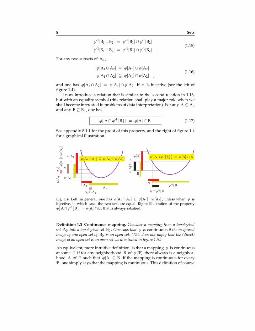
and one has ϕ[A1 ∩A2] = ϕ[A1]∩ ϕ[A2] if ϕ is injective (see the left offigure 1.4).
I now introduce a relation that is similar to the second relation in 1.16,but with an equality symbol (this relation shall play a major role when weshall become interested in problems of data interpretation). For any A ⊆ A0and any B ⊆ B0 , one has
ϕ[ A∩ ϕ-1[ B ] ] = ϕ[A] ∩B . (1.17)
See appendix 8.1.1 for the proof of this property, and the right of figure 1.4for a graphical illustration.
A
B
Fig. 1.4. Left: in general, one has ϕ[A1 ∩A2] ⊆ ϕ[A1]∩ ϕ[A2] , unless when ϕ isinjective, in which case, the two sets are equal. Right: illustration of the propertyϕ[ A∩ ϕ-1[ B ] ] = ϕ[A] ∩B , that is always satisfied.
Definition 1.3 Continuous mapping. Consider a mapping from a topologicalset A0 into a topological set B0 . One says that ϕ is continuous if the reciprocalimage of any open set of B0 is an open set. (This does not imply that the (direct)image of an open set is an open set, as illustrated in figure 1.5.)
An equivalent, more intuitive definition, is that a mapping ϕ is continuousat some P if for any neighborhood B of ϕ(P) there always is a neighbor-hood A of P such that ϕ[A] ⊆ B . If the mapping is continuous for everyP , one simply says that the mapping is continuous. This definition of course

1.2 Mappings 9
applies to metric manifolds, with the topology induced by the metric. Thenotion of continuity also applies to mappings between discrete sets, but itthen has little interest7.
Fig. 1.5. A continuous mapping is defined by thecondition that the reciprocal image of a open setmust be an open set. It is not true the (direct)image of an open set —through a continuousmapping— is an open set: in this example, A isa open set, but its image B = ϕ[A] is a closedset.
A
B
( )
[]
Definition 1.4 Measurable mapping. Consider a mapping from a measurableset A0 into a topological set B0 . One says that ϕ is measurable if the reciprocalimage of any open set of B0 is a measurable set.
If, in addition, A0 is a topological space, and the measurable sets are itsBorel sets, any continuous function is measurable.
To prepare some notions to be introduced later in the book, we now needto examine how the image (or reciprocal image) of a set can be obtained us-ing indicator functions. Let ϕ be a mapping from a set A0 into a set B0 .For any A ⊆ A0 , we have introduced the indicator function χA(a) in equa-tion 1.8. The indicator function of the image set ϕ[A] , that we shall denoteξϕ[A] , then satisfies
ξϕ[A](b) =
1 if b ∈ ϕ[A]0 if b /∈ ϕ[A] .
(1.18)
Let us now turn to the problem of characterizing the indicator function ofthe reciprocal image of a set. Let ϕ be a mapping from a set A0 into a setB0 , B a subset of B0 , and ξB the indicator function of B . It is easy to seethat the indicator function of the set ϕ-1[ B ] ⊆ A0 can then be written (forany element a ∈ A0 )
χϕ-1[ B ](a) = ξB( ϕ(a) ) . (1.19)
For later use, let us also express the indicator function of a set A∩ ϕ-1[B] .Using the second of equations 1.9 and the equation just expressed one ob-tains
χA∩ ϕ-1[B](a) = χA(a) ξB(ϕ(a)) . (1.20)
7 A mapping between two discrete sets with a finite number of elements is alwayscontinuous.

10 Sets
Also, writing relation 1.17 in terms of indicator functions gives, for any el-ement b , ξϕ[A∩ ϕ-1[B]](b) = ξϕ[A] ∩B(b) . Using the second of equations 1.9and equation 1.19 we can express this common value as
ξϕ[A∩ ϕ-1[B]](b) = ξϕ[A] ∩B(b) = ξϕ[A](b) ξB(b) , (1.21)
where ξϕ[A](b) is expressed in equation 1.18.
1.3 Assimilation of Observations
1.3.1 Method
Many problems in the physical sciences correspond to the following situa-tion. There is a first set A0 (with elements denoted a, a′ . . . ), a second setB0 (with elements denoted b, b′ . . . ), and a mapping ϕ from A0 into B0 ,and
(i) we are interested in identifying a particular element a ∈ A0 , and we havethe “a priori information” that it belongs to a subset A1 ⊆ A0 :
a ∈ A1 , (1.22)
(ii) we have “observed” that some element b ∈ B0 belongs to a subset B1 ⊆B0 :
b ∈ B1 , (1.23)
and (iii) we know that b is related to a via the mapping ϕ :
b = ϕ(a) . (1.24)
These three pieces of information, when put together, allow to infer:
(i) that the element a belongs, in fact, to a set A2 that is smaller or equalthan the original set A1 ,
a ∈ A2 ; with A2 = A1 ∩ ϕ-1[B1] ⊆ A1 , (1.25)
(ii) while the element b belongs, in fact, to a set B2 that is smaller or equalthan the original set B1 ,
b ∈ B2 ; with B2 = ϕ[A1]∩B1 ⊆ B1 . (1.26)
These two results are obvious (see, nevertheless, the discussion in fig-ure 1.6). Perhaps less obvious is the relation
B2 = ϕ[A2] . (1.27)

1.3 Assimilation of Observations 11
Fig. 1.6. As b = ϕ(a) belongs to B1 , then,by definition of reciprocal image of a set,the element a must belong to ϕ-1[B1] . Asa also belongs to A1 , it must belong toA2 = A1 ∩ ϕ-1[B1] . Also, as a belongs toA1 , then, by definition of image of a set,the element b = ϕ(a) belongs to ϕ[A1] .As b also belongs to B1 , it must belong toB2 = ϕ[A1]∩B1 .
A0
A0
B0
B0
a a bb
a b
It follows directly from the general property ϕ[ A∩ ϕ-1[ B ] ] = ϕ[A]∩B(equation 1.17, demonstrated in appendix 8.1.1 ).
Remark that we are inside the paradigm typical of a “problem of assim-ilation of observations” —sometimes called “inverse modeling problem”—:the mapping a 7→ b = ϕ(a) can be seen as the typical mapping between the“model parameter space” and the “observable parameter space”. In whatconcerns the element a ∈ A0 we pass from the “a priori information”a ∈ A1 ⊆ A0 to the “a posteriori information” a ∈ A2 ⊆ A1 ⊆ A0 .Similarly, in what concerns the element b ∈ B0 we pass from the “initialobservation” b ∈ B1 ⊆ B0 to the “refined observation” b ∈ B2 ⊆ B1 ⊆ B0 .Working with sets —instead of working with probabilities— corresponds tothe “interval estimation philosophy” that some authors prefer8.
1.3.2 Example
A factory produces screens, that are characterized by two quantities, the sur-face S , and the aspect ratio R (defined as the ratio between the width andthe height). It is known that the screens produced by this factory may havevalues of the surface and of the aspect ratio that satisfy the two constraints
Smin < S < Smax ; Rmin < R < Rmax . (1.28)
For a given screen, and to better know these two values S, R , three in-dependent measurements are performed, the width W of the screen, theheight H , and the diagonal D . These measurements, performed with finiteaccuracy instruments, produce the following results:
Wmin < W < Wmax ; Hmin < H < Hmax ; Dmin < D < Dmax .(1.29)
8 E.g., Stark (1992, 1997).

12 Sets
When taking into account these observations, what can be said about thepossible values of the surface S and of the aspect ratio R of the screen(better than what is in inequalities 1.28)? What can we then say about thepossible values of W , H , and D (better than what is in inequalities 1.29)?As a numerical application, take Smin = 2.6 m2 , Smax = 3.2 m2 , Rmin =1.20 , Rmax = 1.45 , Wmin = 1.9 m , Wmax = 2.1 m , Hmin = 1.4 m , Hmax =1.6 m , Dmin = 2.4 m , and Dmax = 2.6 m .
Solution:
Consider a space A0 , “the space of all possible shapes of screens”. Eachpoint a = S, R ∈ A0 represents a particular shape of screen. The “a pri-ori information” we have on the screen corresponds to the set A1 ⊂ A0 ,defined by the inequalities 1.28, that is represented at the left of figure 1.7.Each possible value of the three observable quantities b = W, H, D de-fines a point in “the space of all possible observations”, say B0 . The (finiteaccuracy) measurement of b = W, H, D produces the set B1 ⊂ B0 , de-fined by the inequalities 1.29, that is represented at the left of figure 1.8.
2.4 2.6 2.8 3 3.2 3.4
1.1
1.2
1.3
1.4
1.5
1.6
2.4 2.6 2.8 3 3.2 3.4
1.1
1.2
1.3
1.4
1.5
1.6
2.4 2.6 2.8 3 3.2 3.4
1.1
1.2
1.3
1.4
1.5
1.6
S S S
R R R
s =
2.6
m2
s =
3.2
m2
w = 1.9 m
r = 1.20
r = 1.45
w = 2.1 m
h = 1.
4 m
d = 2.4 m
h = 1.6 m
d = 2.6 m
Fig. 1.7. The set A1 , the reciprocal image ϕ-1[B1] , and the intersection A2 =A1 ∩ ϕ-1[B1] .
As, by definition of surface and of aspect ratio, S = W H and R =W/H , and as the diagonal is D =
√W2 + H2 , we have
W(S, R) =√
S R
H(S, R) =√
S/R
D(S, R) =√
S (R + 1/R) .
(1.30)
So, given any particular screen a = S, R we can compute the observableb = W, H, D via the equations just written. These equations thus define amapping
a 7→ b = ϕ(a) (1.31)

1.3 Assimilation of Observations 13
from A0 into B0 . This mapping ϕ is not invertible: given an element b ∈ B0we can not compute an a ∈ A0 (each pair of the three quantitities b =W, H, D would define an element a = S, R , so the three quantities inb together may not define any element a ).
Some easy computations allow to represent the set ϕ-1[B1] (middle offigure 1.7), and, then the set A2 = A1 ∩ ϕ-1[B1] (right of figure 1.7) is thesolution to the problem: we now know that the actual screen must belong tothe set A2 . On the observable parameter set B0 we can represent B1 , ϕ[A1] ,and B2 = B1 ∩ ϕ[A1] (figure 1.8). The set B2 represents our final informa-tion of the values of the observable parameters. Because of relation 1.17, weknow that B2 = ϕ[A2] .
1.81.9
22.1
2.21.3
1.41.5
1.61.7
2.3
2.4
2.5
2.6
2.7
1.81.9
22.1
2 2WH
D
1.81.9
22.1
2.21.3
1.41.5
1.61.7
2.3
2.4
2.5
2.6
2.7
1.81.9
22.1
2 2WH
D
1.81.9
22.1
2.21.3
1.41.5
1.61.7
2.3
2.4
2.5
2.6
2.7
1.81.9
22.1
2 2WH
D
B1 (suggested only)
Fig. 1.8. At the left, the set B1 , defined by the conditions 1.9 m < W < 2.1 m ,1.4 m < H < 1.6 m , and 2.4 m < D < 2.6 m . At the middle, the set ϕ[A1] . Atthe right, this same set, together with the set B1 . The intersection of the two sets,B2 = ϕ[A1]∩B1 equals the image of A2 , ϕ[A2] .
So far, we have reasoned on sets, and have plotted sets. But there is amuch faster way of solving this problem: using indicator functions and com-puter plotting routines. Introducing the box function
b(x; x1, x2) =
1 if x1 < x < x2
0 otherwise ,(1.32)
the indicator of the set A1 is
χA1(S, R) = b(S; Smin, Smax) b(R; Rmin, Rmax) , (1.33)
while the indicator of the set B1 is
ξB1(W, H, R) = b(W; Wmin, Wmax) b(H; Hmin, Hmax) b(D; Dmin, Dmax) .(1.34)
The indicator of ϕ-1[B1] is (equation 1.19)
χϕ-1[B1](S, R) = ξB1( W(S, R) , H(S, R) , D(S, R) ) , (1.35)

14 Sets
where the three functions w(S, R) , h(S, R) , and d(S, R) are those in equa-tion 1.30. Finally, the indicator of the set A2 = A1 ∩ ϕ-1[B1] is (second ofequations 1.9)
χA2(S, R) = χA1(S, R) χϕ-1[B1](S, R) . (1.36)
So, in total, the indicator function χA2(S, R) is given by the following prod-uct of box functions:
χA2(S, R) = b(S; Smin, Smax) b(R; Rmin, Rmax)b( W(S, R) ; Wmin , Wmax ) b( H(S, R) ; Hmin , Hmax )b( D(S, R) ; Dmin , Dmax ) .
(1.37)
The three functions χA1(S, R) , χϕ-1[B1](S, R) , and χA2(S, R) are immediateto code on a computer (the code is in figure 1.9) and can be plotted usingany plotting routine. The results, displayed in figure 1.10, are essentiallyidentical to those in figure 1.7, but now immediate to obtain.
Fig. 1.9. The computer code actually used to solve this problem in terms of indi-cator functions. When plotting the three functions χA1 (S, R) , χϕ-1[B1](S, R) , andχA2 (S, R) thus defined, one obtains the drawings in figure 1.10. A commercial soft-ware (mathematica) has been used.
2.6 3 3.41.0
1.2
1.4
1.6
2.6 3 3.41.0
1.2
1.4
1.6
2.6 3 3.41.0
1.2
1.4
1.6
SSS
R R R
Fig. 1.10. Same as figure 1.7, working here with the indicator functions of the sets (theplotting routine used draws zero values as white and unit values as black). To obtainthis figure one needs a very simple computer program (like the one in figure 1.9) anda plotting software.

2 Probabilities
While common theories aimed at the interpretation of observations arebased on the Bayes theorem, I choose here to complete the standard prob-ability theory by adding new definitions and theorems. The basic notionsare the intersection of two probabilities, and —when a mapping betweentwo spaces is introduced— the image and reciprocal image of a probabil-ity. These are generalizations of the corresponding notions in set theory, andsome fundamental properties of set theory are preserved (i.e., they are nowalso valid in probability theory). The theory developed in this chapter is ap-plied in chapter 4 to some typical inference problems in physics (transport ofuncertainties in measurements, assimilation of observations, etc.). When de-veloping the theory, I mention some of the difficulties with the conventionalapproach (for instance, a conditional probability density can only be intro-duced if the manifold under consideration has a metric defined, a difficultyoften overlooked).
2.1 Basic Definitions
To introduce the notion of probability, one can take different approaches.One may, for instance, follow Jaynes (2003) ideas, or one may start fromthe notion of random algorithm (i.e., of algorithm that produces randomoutputs), to obtain as properties the usual axioms of the theory. I choose tostart the theory in the more traditional way, by just stating the Kolmogorovaxioms (Kolmogorov, 1950).
We shall consider a non-empty set Ω and a collection F of subsets of Ω .We shall see that to any subset A in the collection F , a “probability func-tion” P associates a “probability value” P[A] . We must decide which kindof collections of subsets we wish to consider. We need that both, the emptyset ∅ and the whole set Ω belong to F , and we also need that any fi-nite union and any finite intersection of sets in F gives a set that also is inF . This means that the collection F must be a field (definition in page 4).But, do we wish to also consider infinite unions and infinite intersectionsof sets, in which case the field must also be a σ-field (see page 4)? And,when working with manifolds, do we wish to face sets with complex def-initions that may not belong to the Borel σ-field (see page 5) of the mani-

16 Probabilities
fold? Should the present book be about mathematics, the answer would bepositive. But our goal here is to explore a method for the interpretation of(physical) observations, and any attempt at gaining mathematical general-ity would unnecessarily complicate the development of the method. This iswhy, in what follows, I choose to develop the mathematics rigorously, butwithout attempting to attain maximum generality: we shall assume that wealways work with a field (not necessarily a σ-field ) but we will restrainourselves from taking infinite unions or infinite intersections of sets, or tointroduce sets with complex definitions, to which it may not be possible toassociate any “measure” of any “probability”.
Before defining probability functions, we must define measure functions:the measure of a set typically represents is “size” or its “volume”.
Definition 2.1 Measure. Given a set Ω and chosen a set F of subsets of Ωthat is a field, one calls measure function a mapping M from F into the set ofnon-negative real numbers such that
M[ ∅ ] = 0 , (2.1)
and such that for any two sets of F
M[A1 ∪A2] = M[A1] + M[A2]− M[A1 ∩A2] . (2.2)
The number M[A] is called the measure of the set A .
Definition 2.2 Absolute continuity. Let M1 and M2 be two measure functionson the same set. One says that M2 is absolutely continuous with respect to M1 ,and one writes M2 M1 , if M2[A] is zero for every set A for which M1[A] iszero:
M2 M1 ⇔ M1[A] = 0 ⇒ M2[A] = 0 . (2.3)
When later introducing probability functions over a (field of subsets of a)set Ω , there will often be a particular measure function, that we shall denotewith the letter V , such that (i) for any set A , the quantity V[A] has the intu-itive meaning of “volume” of the set A , and (ii) any other measure function(or probability function) to be introduced over Ω , is absolutely continuouswith respect to V (so any possible measure of a set of zero volume is zero).This deserves an explicit definition:
Definition 2.3 Volume measure. Given a set Ω and chosen a field F of subsetsof Ω , if all measure functions to be considered are assumed to be absolutely contin-uous with a given measure function, we say that one has a volume function overΩ (in fact, over F ), and the letter V is used for this volume function. For any setA ∈ F , the quantity V[A] is the volume of the set A . If V[Ω] is finite, onesays that Ω has a finite volume.

2.1 Basic Definitions 17
Example 2.1 Volume of a discrete set. If the set Ω is discrete, one can take asdefinition of volume of a subset A its cardinality, i.e., the number of its elements:
V[A] = card[A] . (2.4)
This is obviously a measure function, and it is clear that any other measure functionover Ω is absolutely continuous with respect to V .
Example 2.2 Volume of a set on a manifold. To have a meaningful notion ofmeasure of a subset of a (finite-dimensional) manifold, one has to introduce an ad-hoc notion of volume. Consider, for instance, a one-dimensional manifold, whereeach point corresponds to the temperature T of a physical body. Which is the lengthof an interval [T1, T2] ? It can be computed as
`(T1, T2) =∫ T2
T1
dT ω(T) , (2.5)
where ω(T) is some chosen positive function. For instance, in most usual situa-tions, invariance arguments suggest to choose ω(T) = 1/T , in which case
`(T1, T2) = logT2
T1. (2.6)
More generally, on an n-dimensional manifold, with coordinates x1, x2. . . xn(that, in this text, shall typically represent physical quantities), the volume of asubset A of the manifold can always be obtained as
V[A] =∫x1,x2...xn∈A
ε12...n dx1 dx2. . . dxn ω(x1, x2. . . xn) , (2.7)
where the positive function ω(x1, . . . , xn) (warning! positive or negative) repre-sents the volume density of the manifold in the given coordinates. Sometimes,one can directly introduce a “volume element” dV and write the coordinate-freeexpression
V[A] =∫P∈A
dV . (2.8)
It is usually not a trivial task to associate a notion of volume to a (physically defined)manifold (chapter 4 gives some examples of this). Let M now be some other measurefunction. By hypothesis, it is absolutely continuous with respect to the volume func-tion (all measure functions must be). The Radon-Nikodym theorem (Taylor, 1966),then warrants that there is a unique, non-negative function P 7→ m(P) , definedat every point P of the manifold, such that the measure value of any set A can beevaluated as
M[A] =∫P∈A
dV m(P) . (2.9)
While for a mathematician dV is an abstract symbol related to the volume functionA 7→ V[A] , for us this equation means that if the function m is known at every

18 Probabilities
point of the manifold, and if the manifold is divided in cells of equal volume ∆V ,the integral is defined as the limit∫
AdV m(P) ≡ lim
∆V→0∑
P∈A∆V m(P) . (2.10)
The function m , a “volumetric measure” (see appendix 5), is an invariant: its val-ues are not related to any possible choice of coordinates over the manifold. Introduc-ing coordinates, and choosing to integrate as
M[A] =∫x1,x2...xn∈A
ε12...n dx1 dx2. . . dxn m(x1, x2. . . xn) (2.11)
defines another function m(x1, x2. . . xn) , a “measure density”, whose values areintimately related to the coordinates being used (and changes, if the coordinates arechanged, according to the Jacobian rule [see appendix 5]). The two functions arerelated as
m(x1, x2. . . xn) = ω(x1, x2. . . xn) m(x1, x2. . . xn) . (2.12)
It is unfortunate that the difference between the two expressions 2.9 and 2.11 isnot always recognized: mathematicians use the term “density” without respect forthe meaning of this term in the (perhaps old-fashioned) tensor theory recalled inappendix 5, and practitioners of probability theory often fail to realize that two verydifferent functions exist, a scalar and a density (taking, sometimes, the one for theother, as suggested at the end of example 2.8).
Definition 2.4 Probability. Given a set Ω and chosen a set F of subsets of Ωthat is a field, a probability function is a measure function, say P , defined overF such that
P[Ω] = 1 . (2.13)
For a set A ∈ F , the number P[A] is called the probability value of the set A(or simply the probability of the set A ).
Because a probability function is a measure function, for any two sets of F
P[A1 ∪A2] = P[A1] + P[A2]− P[A1 ∩A2] . (2.14)
It follows that for any set A ∈ F , 0 ≤ P[A] ≤ 1 , so a probability functionis a mapping from F into the real interval [0, 1] . Also, if two sets A1 andA2 are complementary (with respect to Ω ), then, P[A2] = 1− P[A1] . Ofcourse, the probability of the empty set is zero: P[ ∅ ] = 0 .
We shall call the triplet Ω,F , P a probability triplet (it is usually calleda probability “space”, but we refrain from using this terminology here1). Let
1 Given the pair Ω,F , we shall consider below the space of all probabilities overΩ,F (that we shall endow with an internal operation, the intersection of prob-

2.1 Basic Definitions 19
Ω,F , P1 and Ω,F , P2 be two probability triplets (i.e., let P1 and P2 betwo possibly different probability functions defined over the same field F ).If for any A ∈ F one has P1[A ] = P2[ A ] then one says that P1 and P2 areidentical, and one writes P1 = P2 .
Example 2.3 If the elements of the set Ω are numerable (or if there is a finitenumber of them), Ω = ω, ω′, . . . , then, for any probability P over F = ℘(Ω) ,there exist a unique set of non-negative real numbers p(ω), p(ω′), . . . such thatfor any A ⊆ Ω
P[A] = ∑ω∈A
p(ω) , (2.15)
and, in particular, ∑ω∈Ω p(ω) = 1 . It is then clear that the p(ω) equals theprobability of a set containing a single element,
p(ω) = P[ω] , (2.16)
so, we shall call the number p(ω) the elementary probability (or, for short, prob-ability) of the element ω . While the function A 7→ P[A] (defined on sets) is theprobability function, we shall call the function a 7→ p(a) (defined on elements)the elementary probability function.
A look at figure 2.1 makes this property obvious. In many practical situa-tions, one does not reason on the abstract function P , that associates a num-ber to every subset, but on the collection of numbers p(ω) , one associatedto each element of the set.
Fig. 2.1. From a practical point of view,defining a probability P over a discreteset Ω = ω1, ω2, . . . consists in as-signing an elementary probability pi =p(ωi) to each of the elements of the set,with ∑i pi = 1 .
p9
p3
p5
p6
p1p1
p2 p4
p7p8
A1
A2
abilities). So, here, what would deserve the name of “probability space” would bea given Ω , a given σ-field F ⊆ ℘(Ω) and the collection of all the probabilitiesover Ω,F . So, to avoid any confusion, we better don’t use the term “probabil-ity space”, and call Ω,F , P a probability triplet. Also, the set Ω is sometimescalled the sample space, while the sets in F are sometimes called events. We do notned to use this terminology here. Let us also choose to ignore what a “randomvariable” could be.

20 Probabilities
Example 2.4 Probability density. Assume that the set Ω is a finite-dimensionalmanifold, and that we choose for F the usual Borel field of Ω . If we endow the man-ifold with some coordinates x1, x2. . . xn , then, by virtue of the Radon-Nikodymtheorem (Taylor, 1966), for any probability function P over F there necessarily ex-ists a (unique) non-negative function f (x1, x2. . . xn) , called probability densityfunction, such that for any A ∈ F ,
P[A] =∫x1,x2...xn∈A
ε12...n dx1 dx2. . . dxn f (x1, x2. . . xn) . (2.17)
In practice, one introduces a probability function over a manifold by introducingthe associated probability density function.
Example 2.5 Volumetric probability. In the context of the previous example,assume that the manifold Ω has a notion of volume defined: V[A] =
∫P∈A dV .
Then, the Radon-Nikodym theorem implies that for any probability function P overF there necessarily exists a (unique) non-negative function f (P) , called volumet-ric probability function, such that for any A ∈ F ,
P[A] =∫P∈A
dV f (P) . (2.18)
Because, a notion of volume exists, then, associated to each coordinate systemx1, x2. . . xn , there is a volume density (see example 2.2) ω(x1, x2. . . xn) thatallows to evaluate a volume as (equation 2.7) V[A] =
∫x1,x2...xn∈A ε12...n dx1 dx2
. . . dxn ω(x1, . . . , xn) . Then, a probability function P can be represented by aprobability density function f (x1, x2. . . xn) , so as to have equation 2.17. Therelation between a volumetric probability (an invariant) and a probability density(a density) is the same as that for a general measure (equation 2.12)
f (x1, x2. . . xn) = ω(x1, x2. . . xn) f (x1, x2. . . xn) . (2.19)
Example 2.6 Lognormal distribution. In example 2.2 it has been suggestedthat, for a Kelvin temperature, ω(T) = 1/T . There are two ways of represent-ing a lognornal “distribution”: by introducing a scalar function, the volumetricprobability
f (T) =1√
2π σexp
(− 1
2
(log
TT0
)2 )(2.20)
or a density function, the probability density
f (T) =1√
2π σ
1T
exp(− 1
2
(log
TT0
)2 ). (2.21)
They are related as f (T) = (1/T) f (T) .

2.1 Basic Definitions 21
From now on, and to simplify the exposition of the theory, when we say“a probability function over a set Ω ”, we shall always mean “a probabilityfunction over a set of subsets of Ω that constitute a field”. And when weconsider a set A ⊆ Ω we always consider, in fact, a set that belongs to theconsidered field of subsets.
Definition 2.5 Homogeneous probability. Assume that a volume measure Vhas been selected over a set Ω associating to every set A ⊆ Ω its volume V[A](the number of elements for a discrete set, or a properly introduced notion of volumefor the sets of a manifold). If V[Ω] is finite, then there is one particular probabilityfunction that to every set A associates a probability value that is proportional tothe volume of the set. We shall call it the homogeneous probability function, andwe shall denote it by the symbol H ,
H[A] =V[A]V[Ω]
. (2.22)
Example 2.7 Homogeneous probability for a discrete set. For a discrete setwith a finite number n of elements, the homogeneous probability function is repre-sented by a constant elementary probability function:
p = 1/n . (2.23)
Example 2.8 Homogeneous probability for a manifold. Consider a finite-dimensional manifold Ω where a notion of volume has been introduced, V[A] =∫
A dV . It is assumed that the total volume V[Ω] is finite. Denoting by P a genericpoint of the manifold, the homogeneous probability function is expressed as
H[A] =∫P∈A
dV h(P) , (2.24)
where h is the homogeneous volumetric probability function, that is just aconstant:
h(P) =1
V[Ω]. (2.25)
This gives H[A] = V[A]/V[Ω] , as it should. If instead of integrating using thevolume element dV one has selected some coordinates, one may integratee (seeappendix 5) using the capacity element ε12...n dx1 dx2. . . dxn , and one may write
H[A] =∫x1,x2...xn∈A
ε12...n dx1 dx2. . . dxn h(x1, x2. . . xn) . (2.26)
Then, if the volume of a set A is evaluated as V[A] =∫x1,x2...xn∈A ε12...n dx1 dx2
. . . dxn ω(x1, x2. . . , xn) , the homogeneous probability density function h(x1,x2. . . , xn) is
h(x1, x2. . . , xn) =ω(x1, x2. . . , xn)
V[Ω]. (2.27)

22 Probabilities
It is a common mistake to assume that a constant probability density may repre-sent a homogeneous probability (unless when using Cartesian coordinates on flatmanifolds).
Note: I have here to (briefly!) introduce the notion of sample element of aprobability function, and the notion of a collection of independent sample ele-ments, and have to say what follows: Let P be a probability function definedover some set A0 and let a1, a2, . . . , aN be a collection of N independentsample elements of P . For any set A ⊆ A0 , let n[A] the number of elementsin the sample that belong to A . If n[A] is large enough,
P[A] ≈ n[A]N
. (2.28)
If one is able the generate “pseudo-random” sample elements of the proba-bility function P , this is sometimes the only available method for (approxi-mately) evaluating the probability value of a set A . This method belongs tothe class of Monte Carlo methods, the numerical methods based on the statis-tical analysis of random (or pseudo-random) generation of results.
Example 2.9 Gaussian probability density. As a special case of finite-dimen-sional manifold, consider a finite-dimensional linear space, say A , with vectorsa1, a2 . . . , endowed with the usual vector operations a1 + a2 and λ a . The Gaus-sian (or normal) probability density is
f (a) =det1/2 W(2π)n/2 exp
(− 1
2 (a− a0)t W (a− a0))
. (2.29)
The symmetric, definite non-negative matrix W is the weight matrix. If W is pos-itive definite, its inverse, C = W-1 is the covariance matrix. A positive definiteweight matrix W defines both, a norm ‖ a ‖ =
√at W a over A and a bijec-
tion between A and its dual A∗ : α = W a . The “change of variables” α = W atransforms the probability density f (a) into the probability density (defined, infact, over the dual space A∗ )
g(α) =det1/2 C(2π)n/2 exp
(− 1
2 (α− α0)t C (α− α0))
, (2.30)
where α0 = W a0 is the dual mean. If the weight matrix W has zero eigenvalues,the probability density g(α) is not defined (the covariance matrix C would haveinfinite eigenvalues). Reciprocally, if the covariance matrix C has zero eigenvalues,the probability density g(α) still makes sense, but it is the the probability densityf (a) that is not defined (the weight matrix W would have infinite eigenvalues).
Example 2.10 Gaussian volumetric probability. The linear space A of the pre-vious example is a metric space if one chooses as a metric over A some positive def-inite weight matrix W0 . There is, then, the volume element dv = W0 dv , where

2.2 Intersection of Probabilities 23
W =√
det W0 and dv = ε12...n da1 da2 . . . dan . Associated to the Gaussian prob-ability density f (a) of equation 2.29 is the Gaussian volumetric probability
f (a) =det1/2(W W-1
0 )(2π)n/2 exp
(− 1
2 (a− a0)t W (a− a0))
. (2.31)
The associated normalizations are∫
dv f (a) =∫
dv f (a) = 1 . Choosing themetric W0 = W gives
f (a) =1
(2π)n/2 exp(− 1
2 (a− a0)t W (a− a0))
. (2.32)
2.2 Intersection of Probabilities
The notion of intersection of sets plays a major role when formulating prob-lems in terms of sets. As far as one can see a probability function definedover a set Ω as a generalization of a subset of Ω , it is natural to ask whathow the intersection of sets generalizes when dealing with probabilities.There will be strong similarities between the intersection of probability func-tions and the intersection of “fuzzy sets” (Zadeh, 1965), but the final equa-tions are not quantitatively equivalent, and the domain of application ofthe two definitions is quite different. In my opinion, some of the problemsthat are generally formulated using the notion of conditional probability(and Bayes theorem) are better formulated using the notion of intersectionof probability functions (Tarantola, 1987). This is true, in particular, for theso-called “inverse problems” (see an example in section 4.4.2).
The intersection of probability functions can only be defined if the vol-ume functions mentioned above has been introduced. One must rememberthat for a discrete set there is always the obvious volume measure (numberof elements), while for a manifold the volume measure has to be specified.As we have seen, if the volume of the whole set is finite, a homogeneousprobability function H can be introduced. Any other probability function isthen necessarily absolutely continuous with respect to H . As we shall see,intersection of probability functions depends fundamentally on this homo-geneous probability function.
Definition 2.6 Intersection of probability functions. Consider a set Ω and agiven field F of subsets of Ω . It is assumed that a volume measure V has been in-troduced over F , and that V(Ω) is finite. The associated homogeneous probabilityfunction is denoted H . One considers the space of all probability functions over Fthat are absolutely continuous with respect to the volume measure V (and, there-fore, with respect to the homogeneous probability function H ). Let P1 and P2 twosuch probability functions, and assume that there exists at least one subset A withfinite volume for which P1[A] 6= 0 and P2[A] 6= 0 . The intersection of the twoprobability functions P1 and P2 is defined through the following set of conditions:

24 Probabilities
– the operation is commutative, i.e., for any two probability functions,
P1 ∩ P2 = P2 ∩ P1 , (2.33)
– the operation is associative, i.e., for any three probability functions,
(P1 ∩ P2)∩ P3 = P1 ∩ (P2 ∩ P3) , (2.34)
– the homogeneous probability function H is a neutral element of the operation,i.e., for any probability P ,
P∩H = H ∩ P = P , (2.35)
– and P1 ∩ P2 is absolutely continuous with respect to P1 and P2 , i.e., for anyA ∈ F ,
P1[A] = 0 OR P2[A] = 0 ⇒ (P1 ∩ P2)[A] = 0 . (2.36)
Replacing the set A in equation 2.36 by its complement with respect to Ωgives one further condition:
P1[A] = 1 OR P2[A] = 1 ⇒ (P1 ∩ P2)[A] = 1 . (2.37)
Note: The examples below demonstrate here that there is at least one so-lution to the previous set of conditions. It remains to prove that this solutionis unique2.
Example 2.11 Intersection of discrete probabilities. Assume that the set Ωis discrete, with a finite number of elements, and that we choose F = ℘(Ω) .Let P1 and P2 be two probability functions, with elementary probability functionsrespectively denoted p1 and p2 . The elementary probability function representingP1 ∩ P2 , that we may denote p1 ∩ p2 , is given, for any element ω ∈ Ω , by
(p1 ∩ p2)(ω) =p1(ω) p2(ω)
∑ω′∈Ω p1(ω′) p2(ω′). (2.38)
It is obvious that with this expression, the four conditions above are satis-fied.
2 For the time being, I have taken the simple example of a set with only twoelements. Denoting by f (x, y) the formula that, in this simple example, ex-presses the intersection, the axioms impose the following conditions: f (x, y) =f (y, x) , f (0, x) = 0 , f (1/2, x) = x , f (1, x) = 1 , f (x, f (y, z)) = f ( f (x, y), z) .One solution of this is the right expression, f (x, y) = x y/(1− x− y + 2 x y) , butI don’t know yet if there are other solutions.

2.2 Intersection of Probabilities 25
Example 2.12 Intersection of volumetric probabilities. Assume that the setΩ is a finite-dimensional manifold, and that we choose for F the usual Borel fieldof Ω . Let P1 and P2 be two probabilities, with volumetric probabilities respectivelydenoted f1 and f2 . The volumetric probability representing P1 ∩ P2 , that we maydenote f1 ∩ f2 , is given, for any point P ∈ Ω , by
( f1 ∩ f2)(P) =1ν
f1(P) f2(P) , (2.39)
where ν is the normalization constant ν =∫P∈Ω dv(P) f1(P) f2(P) . It is differ-
ent from zero, because it follows from the assumptions that there is a set of pointswith finite volume where both f1 and f2 are different from zero.
So we see that the intersection of two probabilities is defined in terms ofthe product of the elementary probabilities, or, on a manifold, the productof volumetric probabilities. At this point we may remember the second ofequations 1.9, defining the intersection of sets in terms of their indicatorfunctions: for any ω ∈ Ω , we had
(χA1 ∩A2)(ω) = χA1(ω) χA2(ω) , (2.40)
an expressions similar to the two equations 2.38 and 2.39, excepted for thenormalization factor that makes no sense for indicator functions.
Example 2.13 Intersection of probability densities. This is the same as theprevious example, but, instead of integrating using the volume element, one in-troduces some coordinates x1, . . . , xn and chooses to use the capacity elementdx1 ∧ · · · ∧ dxn (see examples 2.4 and 2.5). Let, again, P1 and P2 be two proba-bility functions, but, this time, represented by the probability densities f 1 and f 2 .The probability density representing P1 ∩ P2 , that we may denote f 1 ∩ f 2 , is givenby (using x for x1, x2. . . , xn )
( f 1 ∩ f 2)(x) =1ν
f 1(x) f 2(x)ω(x)
, (2.41)
where ν is the normalization constant ν =∫
x∈Ω ε12...n dx1 dx2. . . dxn f 1(x) f 2(x)/ ω(x) . Instead of using the volume density ω , we may use the homogeneous prob-ability density h (see equation 2.27), in which case we obtain
( f 1 ∩ f 2)(x) =1ν
f 1(x) f 2(x)h(x)
, (2.42)
where ν is the normalization constant ν =∫
x∈Ω ε12...n dx1 dx2. . . dxn f 1(x) f 2(x)/ h(x) .

26 Probabilities
Example 2.14 A shipwrecked sailor. Let S represent the surface of the Earth,using geographical coordinates (longitude ϕ and latitude λ ). An estimation of theposition of a floating object at the surface of the sea by an airplane navigator gives aprobability distribution for the position of the object corresponding to the (2D) volu-metric probability f1(ϕ, λ) . By definition, then, the probability that the floating ob-ject is inside some region A of the Earth’s surface is P[A] =
∫A dS(ϕ, λ) f (ϕ, λ) ,
where dS(ϕ, λ) = cos(λ) dϕ dλ . An independent (and simultaneous) estimationof the position by another airplane navigator gives a probability distribution corre-sponding to the volumetric probability f2(ϕ, λ) . How the two volumetric probabil-ities f1(ϕ, λ) and f2(ϕ, λ) should be ‘combined’ to obtain a ‘resulting’ volumetricprobability? The answer is given by the intersection of the two volumetric probabil-ities:
f (ϕ, λ) = ( f1 ∩ f2)(ϕ, λ) =1ν
f1(ϕ, λ) f2(ϕ, λ) , (2.43)
with the normalization constant ν =∫S dS(ϕ, λ) f1(ϕ, λ) f2(ϕ, λ) . Beware:
should we be using, instead the volumetric probabilities, the more common proba-bility densities, the (same) answer would have been expressed as
f (ϕ, λ) = ( f 1 ∩ f 2)(ϕ, λ) =1ν
f 1(ϕ, λ) f 2(ϕ, λ)cos(λ)
, (2.44)
with the normalization constant ν =∫S dϕ dλ f 1(ϕ, λ) f 2(ϕ, λ) / cos(λ) .
Example 2.15 Intersection of two Gaussian distributions. The Gaussianprobability densities and Gaussian volumetric probabilities were introduced in ex-amples 2.9 and 2.10. Consider a first Gaussian distribution, with mean vector a1and covariance matrix C1 , and a second Gaussian distribution, with mean vectora2 and covariance matrix C2 . If the covariance matrices are positive definite, thenwe can introduce
W1 = C-11 ; α1 = W1 a1 ; W2 = C-1
2 ; α2 = W2 a2 . (2.45)
Using simple linear algebra it is possible to show that the intersection of the twoGaussian distributions is also a Gaussian distribution, and that it is characterizedby
W = W1 + W2 ; α = α1 + α2 , (2.46)
or, equivalently, by
C = 12 ( S− (C1 S-1 C1 + C2 S-1 C2) )
a = (a1 + a2)− (C1 S-1 m1 + C2 S-1 m2) ,(2.47)
where S = C1 + C2 . When all the matrices are positive definite, equations 2.46are equivalent to equations 2.47, and one has W = C-1 and α = W v . In moregeneral circumstances, it may well happen that W and v are defined, while C andv are not, or vice-versa (see example in section 2.5.2).
2.3 Image of a Probability 27
2.3 Image of a Probability
Here below I consider a mapping from a set A0 into a set B0 , and I considerprobability functions defined both, over A0 and B0 . We know that proba-bility functions are, in fact, defined over sets of subsets, that are assumedto constitute a field. When introducing here the image of a probability func-tion (and, later on, the reciprocal image of a probability function), we shouldcare, in that the fields over A0 and B0 respectively are consistently cho-sen, so when considering images and reciprocal images of sets in one of thefields, we always get a set inside the other field. Let us assume that this isthe case. If not, we need to restric our consideration to continuous mappings(see definition 1.3, page 8): a mapping is continuous if the reciprocal imageof an open set is an open set. (Note: this argument is preliminary, and I haveto be more serious here.)
Definition 2.7 Image of a Probability Function. Let ϕ be a mapping from aset A0 into a set B0 , and let P be a probability function over A0 . We call imageof the probability P via the mapping ϕ , the probability function over B0 , denotedϕ[ P ] , that to any set B ⊆ B0 associates the probability value
(ϕ[ P ])[ B ] = P[ ϕ-1[ B ] ] . (2.48)
So, in simple words, the image of a probability function (via a mapping ϕ ) issuch that the probability value of any subset B (in the arrival set) equals theprobability value (in the departure set) of the reciprocal image of B (via themapping ϕ ). It is easy to check that we have, indeed, defined a probabilityfunction over B0 (see footnote3).
Example 2.16 Image of a Discrete Probability Function. Let ϕ be a mappingfrom a set A0 into a set B0 , P a probability function over A0 , and Q = ϕ[P]its image. If the sets A0 and B0 are discrete4, the probabilities P and Q can berepresented by two elementary probabilities, say p and q = ϕ[p] . One has5, forany element b ∈ B0 ,
3 One has (ϕ[P])[∅] = P[ ϕ-1[∅] ] = P[∅] = 0 and (as the reciprocal imageof B0 equals the whole A0 ) (ϕ[P])[B0] = P[ ϕ-1[B0] ] = P[A0] = 1 . Finally,for any two sets B1 and B2 (subsets of B0 ), one can successively write (using(i) the definition of image of a probability (equation 2.48), (ii) the first of equa-tions 1.15, (iii) equation 2.14, (iv) the second of equations 1.15, and (v) the defini-tion of image of a probability (again)) (ϕ[P])[B1 ∪B2] = P[ ϕ-1[ B1 ∪B2 ] ] =P[ ϕ-1[ B1]∪ ϕ-1[ B2 ] ] = P[ ϕ-1[ B1] ] + P[ ϕ-1[ B2] ] − P[ ϕ-1[ B1 ]∩ ϕ-1[ B2 ] ] =P[ ϕ-1[ B1] ] + P[ ϕ-1[ B2] ] − P[ ϕ-1[ B1 ∩B2 ] ] = (ϕ[P])[ B1 ] + (ϕ[P])[ B2 ] −(ϕ[P])[ B1 ∩B2 ] , so, all the properties that a probability function must satisfy aresatisfied.
4 See section ?? for probabilities over manifolds.5 As equation 2.48 must hold for any B ⊆ B0 , it must also hold for a set containing
a single element. Therefore, for any b ∈ B0 , q(b) = P[ ϕ-1[ b ] ] , from where

28 Probabilities
q = ϕ[p] ⇔ q(b) = ∑a∈ϕ-1[b]
p(a) . (2.49)
Example 2.17 Figure 2.2 suggests a discrete set A0 = a1, a2, a3 , a discreteset B0 = b1, b2, b3 , and a mapping ϕ from A0 into B0 . To every elementaryprobability p defined over A0 one can associate its image q = ϕ[p] (defined overB0 ) as just introduced. Given the mapping suggested in the drawing, one obtains(using equation 2.49) the results written at the bottom of the figure.
Fig. 2.2. The image of a probability via amapping, Q = ϕ[P] . Illustration for dis-crete sets. Note that from p(a1) + p(a2) +p(a3) = 1 it follows that q(b1) + q(b2) +q(b3) = 1 . p(a1) p(a2) p(a3)
given
q(b1) = p(a1) + p(a2)q(b2) = p(a3)q(b3) = 0
a1
a2
a3
b1
b2b3
A0 B0
Example 2.18 Image of a Probability Density Function (regular case). Con-sider a mapping ϕ from a p-dimensional manifold M into a q-dimensional man-ifold N . Take some coordinates x ≡ xi, . . . , xp over M and some coordinatesy ≡ yi, . . . , yq over N . Let P be a probability function over M , representedby the probability density function f (x) , and let Q = ϕ[P] be the image of P viathe mapping ϕ . If p ≥ q , the probability function Q = ϕ[P] can be representedby a bona-fide probability density function, say (ϕ[ f ])(y) . If p = q the problemof evaluating (ϕ[ f ]) is similar to the problem of changing the coordinates on themanifold M (i.e., similar to a problem of “change of variables”), and one easilyobtains
g = ϕ[ f ] ⇔ g(y) = ∑x∈ϕ-1[y]
f (x)|det Φ(x)| , (2.50)
where the Jacobian matrix Φiα = ∂yi/∂xα has been introduced. The sum over all
the x such that ϕ(x) = y is there because the mapping ϕ is not necessarily injec-tive. When p > q , the evaluation of the value g(y) requires an integration of thevalues taken by f (x) in the whole submanifold that maps into the single point x .The simplest way to perform this integration is by introducing some “slack vari-ables” whose integration provides the desired result. For instance, to the original qvariables y we can add p− q variables z ≡ z1, z2, . . . , zp−q that are arbitraryfunctions of the variables x :
the relation 2.49 follows. Alternatively, the direct demonstration is as follows:(ϕ[P])[B] = ∑b∈B(ϕ[p])(b) = ∑b∈B ∑a∈ϕ-1[b] p(a) = ∑a∈ϕ-1[B] p(a) = P[ϕ-1[B]] .

2.3 Image of a Probability 29
y = ϕ(x) (q equations)z = φ(x) (p− q equations) ,
(2.51)
so we now have p equations on the p variables x . As we have the freedom of choiceof the functions φ , they can usually be chosen such that the complete mapping isinvertible, so we can solve the system to get the functions x = x(y, z) . Then, atany point y ∈ N ,
g = ϕ[ f ] ⇔
g(y) =∫
ε12...(p−q) dz1 dz2 . . . dzp−q f (x(y, z))|det Φ(x(y, z))| ,
(2.52)
where the Jacobian matrix Φ contains the partial derivatives of the augmentedmapping in equation 2.51. (Note: I have to demonstrate somewhere that this resultis independent of the choice of the functions φ ). A numerical example of such acalculation is provided in appendix 8.2.1. If the manifolds into consideration havea volume measure function defined, one can introduce two volume densities ωx(x)and ωy(y) , and two volumetric probabilities f (x) = f (x)/ωx(x) and g(y) =g(y)/ωy(y) . Equation 2.52 can then be rewritten so as to give the image of a avolumetric probability function,
g = ϕ[ f ] ⇔
g(y) =∫
ε12...(p−q) dz1 dz2 . . . dzp−q f (x(y, z)) α(x(y, z)) ,(2.53)
where the function
α(x) =ωx(x)
ωy(ϕ(x)) |det Φ(x)| (2.54)
is independent of the particular f (x) under examination.
Example 2.19 Image of a Probability Density Function (singular case).If p < q , the probability density (ϕ[ f ])(y) is singular (it takes zero valueseverywhere, excepted on a p-dimensional submanifold of the q-dimensional man-ifold N ). It is then better to directly work with the definition (equation 2.48). Con-sider a mapping ϕ from a p-dimensional manifold M into a q-dimensional man-ifold N . Take some coordinates x ≡ xi, . . . , xp over M and some coordinatesy ≡ yi, . . . , yq over N . Let P be a probability function defined over M , repre-sented by the probability density function f (x) , and let Q = ϕ[P] the probabilityfunction over N that is the image of P via the mapping ϕ . The probability func-tion Q is represented by some probability density function g(y) . Assume that forsome set B ⊆ N we wish to compute the probability value
Q[B] =∫
y∈Bε1...q dy1. . . dyq g(y) . (2.55)

30 Probabilities
Of course, one could derive the expression of g(y) (as in equation 2.52) and per-form the integral, but there is an easier way. By definition of image of a probability(equation 2.48)
Q[B] = P[ ϕ-1[B] ] =∫
x∈ϕ-1[B]ε1...p dx1. . . dxp f (x) . (2.56)
Typically, the set B has a simple “shape”, but depending on the nonlinearities ofthe mapping ϕ , the shape of ϕ-1[B] can be quite complex. In this situation, oneshould remark that —on a computer— it is quite easy to define the function (anunnormalized density over M )
ψ(x) =
f (x) if ϕ(x) ∈ B
0 otherwise .(2.57)
Then,Q[B] =
∫x∈M
ε1...p dx1. . . dxp ψ(x) , (2.58)
and the domain of integration is the whole manifold M .
Equation 2.52 gives the image in terms of probability densities. Replac-ing them by volumetric probabilities gives the equivalent result
g = ϕ[ f ] ⇔ g(y) = ∑x∈ϕ-1[y]
f (x) ωx(x) / ωy(ϕ(x))√det(Φ(x) Φ(x)t)
, (2.59)
an expression that we must keep ready for later developments. When themanifolds are metric, letting Γ-1 = Γαβ be the contravariant metric overM , and γ-1 = γij the contravariant metric over N , one easily arrives at
g(y) = ∑x∈ϕ-1[y]
f (x)√
det γ(ϕ(x))-1√det(Φ(x) Γ(x)-1 Φ(x)t)
. (2.60)
In many applications, Monte Carlo computations greatly simplify theproblems, and this is true here. We have briefly reviewed in page 22 the no-tion of sample element of a probability distribution. the following propertyshows that the use of a Monte Carlo method trivializes the problem of char-acterizing the image of a probability function via a mapping (note: propertyto be demonstrated in the appendices):
Property 2.1 Let ϕ be a mapping from a set A0 into a set B0 , and let P be aprobability over A0 . If a1, a2, . . . is a collection of independent sample elementsof P , then, ϕ(a1), ϕ(a2), . . . is a collection of independent sample elements ofϕ[P] .

2.4 Reciprocal Image of a Probability 31
This property has both a conceptual and a practical importance. Conceptu-ally, because it gives an intuitive understanding of the notion of transportof a probability function. Practically, because, to obtain a sample of ϕ[p] ,one should not try to develop an ad-hoc method based on the explicit ex-pressions associated to ϕ[P] (like the expression for ϕ[p] in equation 2.49).One should rather obtain a sample of P , and then just map the sample assuggested by property 2.1.
Example 2.20 Image of a Gaussian distribution. Consider a linear mappingL from a p-dimensional linear space A into a q-dimensional linear space B . Theimage (via L ) of a Gaussian distribution in A with mean a0 and covariance Cais the Gaussian distribution in B with mean b0 = L a0 and covariance Cb =L Ca Lt . When p ≥ q , the matrix L Ca Lt may be invertible, in which case theweight matrix Wb = C-1
b exists. When p < q , Cb is not invertible, and theweight matrix is not defined.
2.4 Reciprocal Image of a Probability
Given any two probability functions defined on a set, we have introducedtheir intersection. Also, given a mapping ϕ from a set A0 into a set B0 ,to any probability function P over A0 we have associated its image, ϕ[P]that is a probability function over B0 . Now, the question is: can we associateto any probability function Q over B0 , a probability function, say ϕ-1[Q] ,over A0 deserving the name of reciprocal image of Q ?
One condition must be the consistency with the definition of reciprocalimage of a set, so that the support of ϕ-1[Q] must equal the reciprocal imageof the support of Q , but this condition is easy to fulfill, so we need to turninto a more demanding condition. It is provided by the following
Property 2.2 Let ϕ be a mapping from some set A0 into some other set B0 ,P be a probability function defined over A0 , and Q a probability function definedover B0 . For any mapping ϕ , and any probabilities P and Q , there is a uniqueprobability function over A0 , denoted ϕ-1[Q] , such that
ϕ[ P∩ ϕ-1[Q] ] = ϕ[ P ]∩Q . (2.61)
The (still uncomplete!) demonstration of this property is in appendix 8.1.2(in fact, the demonstration is only valid in two cases, when the sets are dis-crete, and when the sets are manifolds; general demonstration still in con-struction).
Definition 2.8 The ϕ-1[Q] of the property above shall be called the reciprocalimage of P (with respecto the the mapping Q ).

32 Probabilities
We may remember here the relation 1.17, demonstrated in chapter 1:when A and B are sets, ϕ[A] and ϕ-1[ B ] respectively denote the imageand the reciprocal image of a set, and C1 ∩C2 denotes the intersection oftwo sets, one has
ϕ[ A∩ ϕ-1[ B ] ] = ϕ[A] ∩B . (2.62)
This is the exact analogue of equation 2.61. When the probabilities P andQ are only nonzero inside sets A ⊆ A0 and B ⊆ B0 respectively, theprobability ϕ[ P∩ ϕ-1[ Q ] ] = ϕ[P] ∩Q is only nonzero inside the setϕ[ A∩ ϕ-1[ B ] ] = ϕ[A] ∩B . So, the probability theory equation 2.61 con-tains the set theory equation 2.62, and, in this sense, it is a generalization ofit.
Example 2.21 Reciprocal Image of a Discrete Probability Function. Let ϕbe a mapping from a set A0 into a set B0 , Q a probability function over B0 , andP = ϕ-1[Q] its reciprocal image. If the sets A0 and B0 are discrete the probabilitiesQ and P can be represented by two elementary probabilities, say q and p =ϕ-1[q] . One has (demonstration in appendix 8.1.2.1), for any element a ∈ A0 ,
p = ϕ-1[q] ⇔ p(a) =1ν
q( ϕ(a) ) , (2.63)
where ν is the normalization constant ν = ∑a∈A0q( ϕ(a) ) .
Example 2.22 Figure 2.3 suggests a discrete set A0 = a1, a2, a3 , a discrete setB0 = b1, b2, b3 , and a mapping ϕ from A0 into B0 . To every elementary prob-ability q defined over B0 one can associate its reciprocal image p = ϕ-1[q] asjust seen. Given the mapping suggested in the drawing, one obtains (using equa-tion 2.63) the results written at the bottom of the figure.
Fig. 2.3. The reciprocal image of a probability viaa mapping, P = ϕ-1[Q] . Illustration for discretesets.
a3 b2
q(b1) q(b2) q(b3)given
p(a1) = q(b1)/νp(a2) = q(b1)/νp(a3) = q(b2)/ν
ν = 2 q(b1) + q(b2)
a1
a2
b1
A0 B0
b3
Example 2.23 Reciprocal Image of a Volumetric Probability Function. Con-sider a mapping ϕ from a p-dimensional manifold M into a q-dimensional mani-fold N , both manifolds, having a notion of volume defined. Let Q be a probabilityfunction over N , represented by the volumetric probability function g(Q) , and let

2.5 The Bayes-Popper Problem 33
P = ϕ-1[Q] be the image of Q with respect to the mapping ϕ . The probabilityfunction P = ϕ-1[Q] can be represented by a volumetric probability function, say(ϕ-1[g])(P) . As demonstrated in appendix ??, at any point P ∈ M ,
f = ϕ-1[g] ⇔ f (P) =1ν
g(ϕ(P)) . (2.64)
where ν is the the normalizing constant ν =∫
x∈M dVM g(ϕ(P)) .
Example 2.24 Reciprocal Image of a Probability Density Function. Con-sider a mapping ϕ from a p-dimensional manifold M into a q-dimensional man-ifold N . Take some coordinates x ≡ xi, . . . , xp over M and some coordinatesy ≡ yi, . . . , yq over N . Both manifolds are assumed to have a notion of volumedefined, the volume densities associated to the given coordinates being ωx(x) andωy(y) respectively (the notion of volume density was introduced in equation 2.7).Let Q be a probability function over N , represented by the probability densityfunction g(y) , and let P = ϕ-1[Q] be the image of Q with respect to the map-ping ϕ . The probability function P = ϕ-1[Q] can be represented by a probabilitydensity function, say (ϕ-1[g])(x) . It is immediate to see that the expression equiv-alent to 2.64 is
f = ϕ-1[g] ⇔ f (x) =1ν
g(ϕ(x))ωx(x)
ωy(ϕ(x)), (2.65)
where ν is the the normalizing constant ν =∫
x∈M ε12...n dx1dx2. . . dxn g(ϕ(x))ωx(x) / ωy(ϕ(x)) .
Example 2.25 Reciprocal Image of a Gaussian distribution. Consider a lin-ear mapping L from a p-dimensional linear space A into a q-dimensional linearspace B . The reciprocal image (with respect to L ) of a Gaussian distribution in Bwith dual mean β0 and weight matrix Wb is the Gaussian distribution in Awhose weight matrix is Wa = Lt Wb L , and whose dual mean is α0 = Lt β0 .When p ≤ q , the matrix Lt Wb L may be invertible, in which case the covariancematrix Ca = W-1
a exists, and the mean (of the reciprocal image of the originalGaussian) is a0 = Ca α0 . When p > q , Wa is not invertible, and the covariancematrix and the mean vector of the reciprocal image of a Gaussian distribution arenot defined.
Note: mention here figure 2.5.
2.5 The Bayes-Popper Problem
2.5.1 Method
Consider two discrete sets A0 and B0 , a probability function P1 over A0and a probability function Q1 over B0 . As usual, associated to the two prob-ability functions P1 and Q1 there are two elementary probability functionsp1 and q1 such that for any subsets A ⊆ A0 and B ⊆ B0 ,

34 Probabilities
Fig. 2.4. For discrete probabilities, (ϕ-1[ ϕ[p] ])(a) = 1
ν ∑a′∈ϕ-1[ ϕ(a) ] p(a′) , where ν is thenormalization constant ν = ∑a∈ϕ-1[ϕ[A0]] p(a) .Here, p′ = ϕ-1[ ϕ[p] ] .
p(a1) p(a2) p(a3)given (ϕ[p])(b1) = p(a1) + p(a2)
(ϕ[p])(b2) = p(a3)(ϕ[p])(b3) = 0
p’(a1) = ( p(a1) + p(a2) )/νp’(a2) = ( p(a1) + p(a2) )/ν
p’(a3) = p(a3)/ν ν = 2 p(a1) + 2 p(a2) + p(a3)
a1
a2
a3
b1
b2b3
A0 B0
Fig. 2.5. For discrete probabilities,( ϕ[ ϕ-1[q] ] )(b) = 1
ν n(b) q(b) , wheren(b) is the number of elements in A0 thatmap into the element b (i.e., the measureof the set ϕ-1[b] ), and where ν is thenormalization constant ν = ∑b∈B0
n(b) q(b) .Here, q′ = ϕ[ ϕ-1[q] ] .
q(b1) q(b2) q(b3)given(ϕ-1[q])(a1) = q(b1)/ν
(ϕ-1[q])(a2) = q(b1)/ν(ϕ-1[q])(a3) = q(b2)/ν
ν = 2 q(b1) + q(b2)q’(b1) = 2 q(b1)/νq’(b2) = q(b2)/ν
q’(b3) = 0
a1
a2
a3
b1
b2b3
A0 B0
P1[A] = ∑a∈A
p1(a) ; Q1[B] = ∑b∈B
q1(b) . (2.66)
Consider also that a mapping ϕ from A0 into B0 has been introduced.Imagine then that one plays the following game:
1. a random element a ∈ A0 is generated that is a sample element6 of P1 ;2. independently of this, a random element b ∈ B0 is generated that is a
sample element of Q1 ;3. if b 6= ϕ(a) the pair is discarded, and one goes back to point (1);4. if b = ϕ(a) , the pair a, b is accepted, and the game is over.
Questions:
– of which probability function is the element a ∈ A0 —so obtained— asample element?
– of which probability function is the element b ∈ B0 —so obtained— asample element?
– how are these two probability functions related?
The answers (demonstration in appendix 9.1) are as follows. The elementa ∈ A0 is a sample element of the probability function
6 The random element a is sample element of the elementary probability functionp1 if the probability of being selected equals p1(a) .

2.5 The Bayes-Popper Problem 35
P2 = P1 ∩ ϕ-1[Q1] , (2.67)
while the element b ∈ B0 is a sample element of the probability function
Q2 = Q1 ∩ ϕ[P1] . (2.68)
The compatibility property (equation 2.61) then shows that the probabilityfunction Q2 is the image of P2 :
Q2 = ϕ[P2] . (2.69)
The two equations 2.67 and 2.68 are here the demonstrable solutionsto the proposed game. But they are also the solutions of a rather different“game”.
In chapter 3, I formally introduce the notion of “finite-accuracy measur-ing instrument”. Here is, in brief, what I propose there. Although the no-tion applies to discrete sets as well as to manifolds, let us now considerthe case when we deal with manifolds. A particular point P0 of a finite-dimensional manifold M is of special interest to us (it has some “label”, orit is the only one having some “color”, or whatever), and we try to iden-tify P0 “by measuring its position on the manifold”. The best that a finite-measure measuring instrument can do is to provide, after the measurementact, a probability distribution P over the manifold representing the infor-mation obtained on the position of the point P0 . This probability functionis represented, as usual, by the associated volumetric probability functionf (P) (if the manifold has a notion of volume) or by the associated probabil-ity density function f (x) (if some coordinates x = x1, x2, . . . have beenselected over the manifold). Well established practices for the expressionof uncertainties in measurements (ISO, 1993; Taylor and Kuyatt, 1994) con-sider two universal types of experimental uncertainty, both always present:uncertainties that can be evaluated using statistical methods, and uncertain-ties that can only be evaluated using subjective arguments. When they aresimultaneously taken into account, this results in a probability distribution,and this is exactly the meaning the probability function P just considered.
Consider, then, two finite-dimensional manifolds, M and O (that mayhave different dimensions). We wish to identify some special point M0 ∈M , and some special special point O0 ∈ O , but we only have a finite-accuracy measuring instruments, that provide on M0 the information con-tained in a probability function P1 , and on O0 the information contained ina probability function Q1 . In the absence of any extra piece of information,this is what we have. But if we learn that the point O0 ∈ O is, in fact, theimage of the point M0 ∈ M , via a known mapping ϕ , so O0 = ϕ(M0) , thismodifies the information we had on both, M0 and point O0 . I shall arguewith some detail in chapter 3 that the usual definition of experimental un-certainties is such that the final information one has for the point M0 ∈ Mcorresponds to the probability function

36 Probabilities
P2 = P1 ∩ ϕ-1[Q1] , (2.70)
while the final information one has for the point O0 ∈ N corresponds to theprobability function
Q2 = Q1 ∩ ϕ[P1] , (2.71)
and, again, the compatibility property tells that the probability function Q2is the image of P2 :
Q2 = ϕ[P2] . (2.72)
These are, of course the same as equations 2.67–2.69, but applied here in adifferent context.
There is an important class of “inference problems”, where each pointM of the manifold M represents a possible model of a physical system (note:explain this), and where each point O of the manifold O represents apossible outcome of an observation (note: explain this), and the mappingM 7→ O = ϕ(M) represents the prediction of the observation O associatedto the model M , obtained using the predictive power that, following Pop-per (1934), physical theories must have. These problems receive the nameof inverse problems or of problems of assimilation of observations. I mentionedabove that the uncertainties contaminating any real life measurement havetwo sources: those that can be analyzed using statistical techniques, andthose that have to be introduced using subjective considerations. In the classof problems now considered, the probability function P1 , representing theinformation on the model space manifold M comes from very little of sta-tistical analysis, and from very much of subjective reasoning, in which caseone calls P1 the a priori probability function in the model space M . Then,P2 = P1 ∩ ϕ-1[Q1] is the a posteriori probability function in the model M . Sim-ilarly, we could say that Q1 is the a priori probability function in the observa-tions space O , and that Q2 = Q1 ∩ ϕ[P1] is the a posteriori probability functionin the observations space O .
Although we are using nowhere the Bayes theorem, the very notion ofpassing from a priori probabilities to a posteriori probabilities is clearlyBayesian. Let us now make some developments to see why this approachcan also be called Popperian. To start with, let us write explicitly the a pos-teriori probability P2 = P1 ∩ ϕ-1[Q1] in the two usual cases, where one dealswith discrete sets, and where one deals with manifolds.
For discrete sets, let p1 and q1 be the two elementary probability func-tions representing the two probability functions P1 and P2 . Denoting p2the elementary probability function that represents P2 = P1 ∩ ϕ-1[Q1] , wecan symbolically write
p2 = p1 ∩ ϕ-1[q1] . (2.73)
Using equation 2.63 (reciprocal image of a probability) and equation 2.38(intersection of probabilities), we immediately obtain the explicit expression

2.5 The Bayes-Popper Problem 37
p2(a) =1ν
p1(a) q1(ϕ(a)) , (2.74)
with the normalizing constant ν = ∑a∈A0p1(a) q1(ϕ(a)) . Similarly, denot-
ing q2 the elementary probability function that represents Q2 = Q1 ∩ ϕ[P1] ,we can symbolically write
q2 = q1 ∩ ϕ[p1] , (2.75)
and it is also easy to obtain an explicit expression for q2 (see footnote7), butwe don’t typically need this expression, because we already have an explicitexpression for p2 , and we know that q2 is the image of p2 (see discussionbelow).
For manifolds, let f1 and g1 be the two volumetric probability functionsrepresenting the two probability functions P1 and P2 (in order for the in-tersection to be defined, we need to assume that our manifolds are volumemanifolds). Denoting f2 the volumetric probability function that representsP2 = P1 ∩ ϕ-1[Q1] , we can symbolically write
f2 = f1 ∩ ϕ-1[g1] . (2.76)
Using equation 2.65 (reciprocal image of a probability) and equation 2.39(intersection of probabilities), we immediately obtain the explicit expression
f2(P) =1ν
f1(P) g1(ϕ(P)) , (2.77)
with the normalizing constant ν =∫P∈M dvM f1(P) g1(ϕ(P)) . Similarly,
denoting g2 the elementary probability function that represents Q2 =Q1 ∩ ϕ[P1] , we can symbolically write
g2 = g1 ∩ ϕ[ f1] , (2.78)
but, as we are about to see, we don’t typically need this expression, becausewe already have an explicit expression for f2 , and we know that g2 is theimage of f2 (the expressions are given in appendix XXX)
Let us keep reasoning in the context of a problem of assimilation of ob-servations, where the volumetric probability f1(P) represents some a pri-ori information on a system, g1(O) the information obtained through somefinite-accuracy observations, and M 7→ O = ϕ(M) the association, to ev-ery model M of the system, the prediction of the observation O . The aposteriori information on the system is that represented by the volumetricprobability function f2(P) expressed in equation 2.77. Even when the func-tions f1(P) and g1(O) are simple, the volumetric probability f2(P) can
7 One arrives at q2(b) = (1/ν) q1(b) ∑a∈ϕ-1[b] p1(a) , where ν is the normalizingconstant ν = ∑b∈B0
q1(b) ∑a∈ϕ-1[b] p1(a) .

38 Probabilities
be quite complex, because the mapping M 7→ O = ϕ(P) is usually nonlin-ear8. For this reason the possible use of analytical techniques is quite limited(excepted for some simple examples, as in page XXX). Therefore one is typ-ically reduced to the use of Monte Carlo methods, and we shall now brieflyexplore what this means.
We have already seen above (page XXX) that the sampling of a probabil-ity distribution, if doable with a reasonable amount of computer resources,allows to evaluate the probability of any event. So, when dealing with a gen-eral problems of assimilation of observations, one may reduced to the goalof obtaining a large enough collection of points that are sample points of theposterior volumetric probability f2(P) . One then can proceeds as follows.
1. Use any ad-hoc method9 to generate a random point M ∈ M that is asample point of f1(P) ;
2. evaluate the point O = ϕ(M) (this may require heavy computations, asit corresponds to solving a problem of physical modeling);
3. with the O so obtained, evaluate the numerical value π = g1(O)/K ,where K is any number larger or equal to the maximum value of g1 ,say gmax
1 (the closer K to gmax1 the more efficient the algorithm);
4. decide randomly to accept the point M or to reject it, with a probabilityof acceptance equal to π (note that π is a real number inside the inter-val [0, 1] ). When a point M is accepted in this way, it is a sample point ofthe volumetric probability function f2(M) expressed in equation 2.77.
Note: explain somewhere that is is a simple application of the “rejectionmethod” for sampling a probability (see appendix XXX). I have also to checkif a bona-fide demonstration that this algorithm produces the intended re-sult is in the Mosegaard and Tarantola (1995) paper.
Note: I must now explain here that this approach puts us very near thePopperian falsification paradigm: all models M that have been produced assamples of the prior distribution f1(M) , but have not been accepted whenconsidering the value g1( ϕ(M) ) , have been falsified. Because of this mix-ture of Bayesian point of view (passing from a priori distributions to a pos-teriori distributions) and of Popperian point of view (falsification of models)I have called this approach the Bayes-Popper paradigm (Tarantola, 2006b).
8 In fact, the manifolds M and O are themselves nonlinear manifolds as the exam-ples in XXX and XXX show.
9 See an example of this in page XXX. If no such method is known, then, (i) generatea random point M ∈ M that is a sample of the homogeneous probability functionover M ; (ii) evaluate the numerical value π = f1(M)/K , where K is any numberlarger or equal to the maximum value of f1 , say f max
1 (the closer K to f max1 the
more efficient the algorithm); (iii) decide randomly to accept the point M or toreject it, with a probability of acceptance equal to π (note that π is a real numberinside the interval [0, 1] ). When a point M is accepted in this way, it is easy to seethat it is a sample point of the volumetric probability function f1(M) .

2.5 The Bayes-Popper Problem 39
Note: I must, of course, explain that what Popper had in mind is the fal-sification of theories, while what we have in mind here is, given a theory,the falsification of models of a system, and this is a very different issue. Oneadvantage we have with respect to the problem of falsifying theories is thatthere is not easy to introduce something like an a priori probability distri-bution of theories, while in our problem we do have an a priori probabilitydistribution of models.
2.5.2 Example
Consider a linear mapping L from a p-dimensional linear space A into aq-dimensional linear space B . Assume that over A we have the Gaussianvolumetric probability f1(a) , characterized by the mean vector a0 and thepositive definite covariance matrix Ca , while over B we have the Gaussianvolumetric probability g1(b) , characterized by the mean vector b0 and thepositive definite covariance matrix Cb . To evaluate the volumetric proba-bility
f2(a) = ( f1 ∩ ϕ-1[g1])(a) (2.79)
we just need to collect the results in example 2.25 (reciprocal image of aGaussian) and in example 2.15 (intersection of two Gaussians), to find thatf2(a) is a Gaussian volumetric probability, characterized by the followingcovariance matrix and mean vector:
Ca = (C-1a + Lt C-1
b L)-1 ; a0 = Ca (C-1a a0 + Lt C-1
b b0) . (2.80)
Note that the covariance matrix Ca is regular, whatever are the values pand q (i.e., whatever are the dimensions of the two spaces A and B ), andwhatever the linear operator L is (the sum of a positive definite matrix anda definite non-negative matrix is positive definite). The weight matrix of theGaussian (ϕ-1[g1])(a) is Lt C-1
b L , and this matrix is necessarily singularwhen p > q . To speak grossly, this would mean that the “ellipsoid of un-certainties” associated to (ϕ-1[g1])(a) has infinitely large principal values.This does not cause any problem for making the intersection f1 ∩ ϕ-1[g1]that gives, as already mentioned, a regular Gaussian. The expressions inequation 2.80 correspond to the solution of a “least-squares linear inverseproblem” (see Tarantola [2005], page 66).
To evaluate the volumetric probability
g2(b) = (ϕ[ f1]∩ g1)(b) (2.81)
we could collect the results in example 2.20 (image of a Gaussian) and inexample 2.15 (intersection of two Gaussians), and simplify the expressionsso obtained. It is much simpler to use the compatibility property, that heregives g2 = ϕ[ f2] . Using the result explained in example 2.20 (image of a

40 Probabilities
Gaussian) we then find that g2(b) is the Gaussian distribution whose co-variance matrix and mean vector respectively are
Cb = L Ca Lt ; b0 = L a0 . (2.82)
When p ≥ q , the covariance matrix Cb may be regular. When p < q , Cb isnecessarily singular: at least q− p of the principal values of its “ellipsoid ofuncertainties” are zero.
2.5.3 Example
In the problem analyzed in example 1.3.2 (page 11) all information was interms of sets. Let us now here generalize to the case where we handle prob-ability functions instead of sets (this is generalization because if the initialvolumetric probability functions were box-car functions we would foundthe same results obtained there).
Again, a screen is characterized by its surface S and its aspect ratio R .And the measurements we may perform on a screen are its width W , itsheight H , and its diagonal D . The simplest example of volumetric prob-abilities would here corresponds to the normal (or Gaussian assumption),but, as all these quantities are necessarily positive, the lognormal distribu-tion (see example 2.6) would be mathematically more consistent (as nega-tive values of the quantities are impossible). Alternatively, let us drop thefive positive quantities above, and let us work with their logarithms,
s = logS`
; r = logR`
; w = logW`
; h = logh`
; d = logD`
,(2.83)
where ` is some arbitrary length, that we take equal to the internationalunit of length, ` = 1 m (the results are independent of this choice). Forthose quantities, the 1D volume elements (in fact, length elements) are sim-ply dss(s) = ds , dsr(r) = dr , dsw(w) = dw , dsh(h) = dh , and dsd(d) = dd ,so there is here no difference between probability densities and volumetricprobabilities.
Let us assume that a factory produces random screens, distributed ac-cording to the two-dimensional Gaussian volumetric probability
f1(s, r) =1
2 π σs σrexp
[− 1
2
( (s− s0)2
σ2s
+(r− r0)2
σ2r
) ], (2.84)
where s0 = 1.05 , σs = 0.05 , r0 = 0.27 , and σr = 0.05 . This function isrepresented at the left of figure 2.7.
We now (randomly) take one particular screen, and we measure w , h ,and d , using finite-accuracy measuring instruments. Imagine that the in-struments are noisy in the following simple way: when the actual value of

2.5 The Bayes-Popper Problem 41
the input is x , the output is a random quantity, with a Gaussian distribu-tion centered on x and having a standard deviation σ . Then, if the outputof the instrument is say x0 , the probability distribution for x is a Gaussiancentered on x0 and having σ as standard deviation. So, in this sense, letus assume that the information we obtain, though our three (independent)measurements, on the values of the measured quantities can be expressedby a three-dimensional Gaussian,
g1(w, h, d) =1
(2 π)3/2 σ3 exp[− (w− w0)2 + (h− h0)2 + (d− d0)2
2 σ2
],
(2.85)where w0 = 0.70 , h0 = 0.40 , d0 = 0.90 , and σ = 0.03 .
Note: to evaluate the three quantities w, h, d we just take the logarithmof the equations 1.30 (page 12), to obtain
w(s, r) = (s + r)/2h(s, r) = (s− r)/2d(s, r) = (s + log(2 cosh r))/2 .
(2.86)
Bla, bla, bla, and the posterior probability function over the screen modelspace is
P2 = P1 ∩ ϕ-1[Q1] , (2.87)
or, in terms of the volumetric probabilities,
f2 = f1 ∩ ϕ-1[g1] . (2.88)
Let us defineξ(s, r) = g1( w(s, r) , h(s, r) , d(s, r) ) . (2.89)
Excepted for a normalization factor about which we do not need to care, thisfunction equals the reciprocal image of g1(w, h, d) . The volumetric probabil-ity f2(s, r) we are searching is the intersection of f1(s, r) and ξ(s, r) :
f2(s, r) =1ν
f1(s, r) ξ(s, r) , (2.90)
where ν =∫
A0ds dr f1(s, r) ξ(s, r) . This function is represented in the mid-
dle of figure 2.7.The posterior information we have on the observable parameters is
Q2 = ϕ[P2] = ϕ[ P1 ∩ ϕ-1[Q1] ] = ϕ[P1]∩Q1 , (2.91)
or, in terms of the volumetric probabilities,
g2 = ϕ[ f2] = ϕ[ f1 ∩ ϕ-1[g1] ] = ϕ[ f1] ∩ g1 . (2.92)

42 Probabilities
Fig. 2.6. This is the same problem as that analyzed in example 1.3.2 (page 11), butusing here a probabilistic formulation (and logarithmic parameters). All initial dis-tributions are assumed to be Gaussian. These lines correspond to the computer codeactually used to solve this problem. Note that, excepted for the normalization, thiscode is identical to that used to solve a set theory version of a similar problem (seefigure 1.9). Note: the command If[condition,a,b] returns a if the condition issatisfied, and returns b if the condition is not satisfied (here, the sybol ∧ is thelogical AND).
s s s
r r r
0.9 1 1.1 1.2
0.1
0.2
0.3
0.4
0.9 1 1.1 1.2
0.1
0.2
0.3
0.4
0.9 1 1.1 1.2
0.1
0.2
0.3
0.4
Fig. 2.7. Left: the prior volumetric probability f1(s, r) . Middle: the posterior volu-metric probability f2(s, r) . Right: the function ψ(s, r) whose integral gives the an-swer to the following question: which is the posterior probability that the observableparameters w, h, d belong to the domain w > 0.67 , h > 0.38 , d > 0.90 ?

2.5 The Bayes-Popper Problem 43
Fig. 2.8. The plotting commands.
This volumetric probability g2(w, h, d) is singular in that it is zero ex-cepted on a 2D submanifold of B0 (note: explain this). But, as explained inpage 2.55, there is no difficulty in evaluating the probabilities associated toit, as we, in fact, integrate f2(s, r) . To see an example of this, let us evaluatethe probability of the set B ⊂ B0 defined as
B = w > 0.67 , h > 0.38 , d > 0.90 . (2.93)
Of course, this could be written
Q2[B] =∫w,h,d∈B
dw dh dd g2(w, h, d) , (2.94)
but, more simply, we can write (see page 2.55)
Q2[B] =∫s,r∈A0
ds dr ψ(s, r) , (2.95)
where
ψ(s, r) =
f2(s, r) if ϕ(s, r) ∈ B
0 otherwise .(2.96)
The function ψ(s, r) is represented at the right of figure 2.7. An easy numer-ical integration then gives
Q2[B] = 0.48 . (2.97)
Note: mention that the image of the function f2(s, r) is represented at theleft of figure 2.9. At the right of the figure, there is another way of estimatingthe value Q2[B] .

44 Probabilities
0.65
0.7
0.35
0.4
0.45
0.9
0.95
0.65
0.7
0.35
0.4
0.45
0.65
0.7
0.35
0.4
0.45
0.9
0.95
0.65
0.7
0.35
0.4
0.45
w w
d d
h h
Fig. 2.9. Left: sampling the probability distribution f2(s, r) (using the simple rejec-tion algorithm) and plotting the image points, gives a representation of the imageof f2(s, r) . Right, the points that satisfy w > 0.67 , h > 0.38 , d > 0.90 . The pro-portion of accepted points is ≈ 0.48 , this being another way of estimating the valueQ2[B] .

3 Physical Quantities, Manifolds, and PhysicalMeasurements
prov
ision
alch
apte
r
Although it is commonly assumed that a measurement just provides thevalues of some physical quantities —and attached uncertainties— there isa more general, geometrical interpretation of the measurement act: an at-tempt to obtain information on the position —on an abstract manifold—of the point that represents the system under study. On that abstract man-ifold (here named measurable quality space) the possible equivalent phys-ical quantities that we may choose to use (say, a frequency, or its inverse,a period) appear as different choices of coordinates. When conceptualizingin this way a measurement act, its result is a probability function over amanifold (i.e., over a measurable quality space), this probability functionexisting independently of any coordinate system chosen on the manifold,i.e., not being attached to any particular physical quantity (among the manyequivalent physical quantities one may choose to use). This way of thinkingproduces a theory that has built-in the necessary invariances that any infer-ence theory should have (what we will finally deduce about the propertiesof a system will be independent of the particular physical quantities that wemay choose to use for any numerical computation1).
1 Also, the steps of any numerical algorithm —let it be a Monte Carlo algorithm oran optimization algoritm— will be independent of any special choice of physicalquantities (see chapter 4).

46 Physical Quantities, Manifolds, and Physical Measurements
3.1 Physical Quantities: the Intrinsic Point of View
PRO
VISIO
NA
L
The goal of this book is to develop the method to be used for “assimilat-ing” the results of some measurements (in terms of the properties of somephysical system). Usually, one understands that a measurement measuresthe value of a given physical quantity. But we need to go a little bit beyondthat notion.
Example: the Space of Linear Electric Wires
Assume, for example, that we deal with an electric wire (figure 3.1), that wedenote with the symbol W , and we discover that it satisfies the Ohm law,i.e., in the regime of small electric potential difference U and, therefore, ofsmall current intensity I , the two quantities are proportional, with a coef-ficient of proportionality that is characteristic of the wire. This suggests todefine the electric resistance R of the wire, or, equivalently, the electric con-ductance C of the wire, as
R =UI
; C =I
U, (3.1)
and one has R C = 1 . While the standard unit of resistance is the ohm (Ω) ,the standard unit of conductance is the siemens (S) , the two units beingrelated via Ω S = 1 . If we wish to characterize an electric wire W , shouldwe measure its resistance R or its conductance C ? And, how should weexpress the result of the measurement, with the associated uncertainties?
Bla, bla, bla. . .
Fig. 3.1. What should we measure tocharacterize an electric wire that satis-fies the Ohm’s law? The resistance R ,the conductance C , the cube of the resis-tance, the logarithmic conductance, etc.?One doesn’t measure any of these: onemeasures a potential difference U anda current intensity I (both, unavoidably,with finite accuracy), from where it fol-lows an information on the wire that canbe represented as a probability functionover the “space of all possible electricwires”. Over that one-dimensional man-ifold, one can use the coordinate R , thecoordinate C , etc., but the probabilityfunction is not associated to any of thesein particular.
Electric wire
U = R I ; I = C U
R = ? ; C = ? ; R3 = ?r = ? ; c = ?
Bla, bla, bla. . . (see figure 3.2).

3.1 Physical Quantities: the Intrinsic Point of View 47
RESISTANCE
LOGARITHMIC CONDUCTANCE
CONDUCTANCE
LOGARITHMIC RESISTANCE
0.01 Ω0.001 Ω0.0001 Ω0.00001 Ω 0.1 Ω 1 Ω 10 Ω
100 S1000 S10000 S100000 S 10 S 1 S 0.1 S
−2−4−5 −3 −1 0 +1
+2+4+5 +3 +1 0 −1
Fig. 3.2. To characterize an electric wire, one doesn’t measure its resistance, or itsconductance, but some more basic quantities (for instance, electric potential differ-ence and current intensity). One then obtains an information that can equivalentlybe expressed in terms of resistance, conductance, logarithmic resistance, etc. Usingan obvious metric (see text) in the space of all electric wires allows to represent theresult of the measurement as a (1D) volumetric probability (the trapezoidal functionin the figure), that can be read using any of the common quantities (resistance, con-ductance, logarithmic resistance, etc.). It is when “representing linearly” the metriccoordinates (here the logarithmic resistance and the logarithmmic conductance thatthe expression of uncertainties is the simplest (see text for details).
Example: the Space of Linear Elastic Media
PRO
VISIO
NA
LConsider now the situation when we investigate the properties of a lin-
ear elastic medium, not necessarily isotropic (figure 3.3). A linear elasticmedium is an idealization of some physical elastic media that, when sub-mitted to sufficiently small stresses, undergo a strain that is proportional tothe stress. Then if σij are the components of the stress tensor, and εij thecomponents of the strain tensor, a linear elastic medium satisfies the linearrelation that can be expressed using any of the two equivalent formulas
σij = cijk` εk` ; εij = dij
k` σk` , (3.2)
where cijk` are the components of the stiffness tensor, and dij
k` those of itsinverse, the compliance tensor.
Note: write here the exact relation linking the compliance and the stiff-ness (taking into account the assumed symmetries).
Note: explain here that an elastic medium E is a point in an abstract,21-dimensional manifold (a measurable quality space), the space of linear elasticmedia.
Note: explain here that the distance between two elastic media E1 andE2 , represented by the stiffness tensors c1 and c2 , or, alternatively, by thetwo compliance tensors d1 and d2 , is (note: explain why)

48 Physical Quantities, Manifolds, and Physical Measurements
D(E1, E2) = ‖ log c1 c-12 ‖ = ‖ log d1 d-1
2 ‖ . (3.3)
PRO
VISIO
NA
L
Note: explain that this space has curvature (the Riemann tensor of the man-ifold is non-zero). Note: explain that this space is 21-dimensional symmet-ric submanifold of the Lie group manifold GL+(6) . Note: introduce herethe volume measure of the manifold. Explain that it is, in fact, the Haarmeasure of the Lie Group GL+(6) , well-known by mathematicians, buttypically not introduced in practical applications of probability theory. ThisHaar measure is nothing but the volume element associated to the distancein equation 3.3. For, using the coordinates bla, bla, bla, this finite distancederives from the differential distance element
ds2 = gαβ dxα dxβ (3.4)
and the volume element is then
dV =√
det g dx1 dx2 . . . dx21 . (3.5)
For instance, taking as coordinates the quantities bla, bla, bla, one gets bla,bla, bla.
Bla, bla, bla. . .
Fig. 3.3. To characterize a linear elastic mediumone makes simultaneous measurements of stress andstrain, in sufficient number as to characterize the21 degrees of freedom of the medium (unless themedium is isotropic, in which case there are only twodegreed of freedom). One can choose to express thesedegrees of freedom by expressing 21 independentcomponents of the stiffness tensor cij
k` , or 21 inde-pendent components of the compliance tensor dij
k` ,of the 6 eigenvalues and 15 angles of one of the othertensor, or 21 independent components of the loga-rithm of one or the other tensor, etc.
Elastic anisotropic medium
σij = Cijkl εkl ; εij = Dij
kl σkl
Cijkl = ? ; Dij
kl = ? ; Λα = ?cij
kl = ? ; dijkl = ? ; λα = ?
Bla, bla, bla. . .Bla, bla, bla. . . (see figures 3.4, 3.5, and 3.6).

3.1 Physical Quantities: the Intrinsic Point of View 49
Fig. 3.4. The eigenvalues ofthe stiffness tensor are Q =3 κ and N = 2 µ , where κis the bulk modulus (incom-pressibility), and µ is theshear modulus (inshearabil-ity). Here, C is an arbitraryvalue (with the physical di-mensions of a pressure), andκ and µ are in units of C .Contrary to the coordinatesκ, µ , the (logarithmic) co-ordinates k, m and q, nare Cartesian (see text).
q = +
7
q = +
5
q = +
3
q = +
1
q = −
1
n = −6
n = +4
n = +2
n = 0
n = −2
k = +
4
k = +
2
k = 0
k = −
2
k = −
4
m = +4
m = +2
m = 0
m = −2
m = −4
µ = 50µ = 100
µ = 10
κ =
5
κ =
1
κ =
10
κ =
0.5
κ =
0.1
κ =
0.05
κ =
0.01
µ = 5
µ = 1µ = 0.5
µ = 0.1µ = 0.05
µ = 0.01
κ =
100
κ =
50
k = lo
g κ/C
m = log µ/C
q = lo
g Q/C
n = lo
g N/C
Q = 3 κ
N = 2 µ
q = k+
3
n = m
+3
Fig. 3.5. While the Youngmodulus Y is quite an ordi-nary coordinate (0 < Y <∞) , the Poisson’s ratio νis quite unnatural (−1 <ν < +1/2) , and its inter-est is mainly historical. Here,the coordinates Y, ν, plot-ted together with the Carte-sian coordinates k, m andq, n . The quantity Y isplotted in units of C (see fig-ure 3.4).
q = +
7
q = +
5
q = +
3
q = +
1
q = −
1
n = −6
n = +4
n = +2
n = 0
n = −2
k = +
4
k = +
2
k = 0
k = −
2
k = −
4
m = +4
m = +2
m = 0
m = −2
m = −4
Y = 0.1
Y = 1
Y = 10
Y = 100
ν = −0.95
ν = −0.5
ν = −0.25
ν = 0
ν = −0.25
ν = −0.45
ν = −0.499
ν = −0.999
9 κ µ
3 κ + µY =
3 κ − 2 µ
2 (3 κ + µ)
ν =

50 Physical Quantities, Manifolds, and Physical Measurements
Fig. 3.6. Two points (which istheir distance?) and a volu-metric probability (at whichpoint the volumetric proba-bilty is maximum?).
q = +
7
q = +
5
q = +
3
q = +
1
q = −
1
n = −6
n = +4
n = +2
n = 0
n = −2
k = +
4
k = +
2
k = −
2
k = −
4
m = +4
m = +2
m = 0
m = −2
m = −4
k = 0
3.2 Expressing the Results of Measurements 51
3.2 Expressing the Results of Measurements
PRO
VISIO
NA
L
Metrology theory, the science of measurement, has two components, thedefinition of good experimental practice, and the description of the uncer-tainties resulting from measurements. We are here concerned with this sec-ond point, and, in this respect, there is a good text2, published by ISO (Inter-national Organization for Standardization). Here are some of the guidancesand recommendations (in slanted characters, the official text, in roman char-acters my comments).
The objective of a measurement is to determine the value of the measur-and, that is, the value of the particular quantity to be measured. A mea-surement therefore begins with an appropriate specification of the measur-and, the method of measurement, and the measurement procedure. Theterm “true value” is not used [. . . ]; the terms “value of a measurand” (or ofa quantity) and “true value of a measurand” (or of a quantity) are viewedas equivalent. [. . . ] In practice, there are many possible sources of uncer-tainty in a measurement, including: a) incomplete definition of the measur-and; b) imperfect realization of the definition of the measurand; c) nonrep-resentative sampling — the sample measured may not represent the definedmeasurand; d) inadequate knowledge of the effects of environmental con-ditions on the measurement or imperfect measurement of environmentalconditions; e) personal bias in reading analogue instruments; f) finite in-strument resolution or discrimination threshold; g) inexact values of mea-surement standards and reference materials; h) inexact values of constantsand other parameters obtained from external sources and used in the data-reduction algorithm; i) approximations and assumptions incorporated in themeasurement method and procedure; j) variations in repeated observationsof the measurand under apparently identical conditions. These sources arenot necessarily independent, and some of sources a) to i) may contribute tosource j). Of course, an unrecognized systematic effect cannot be taken intoaccount in the evaluation of the uncertainty of the result of a measurementbut contributes to its error.
In 1977, the Comité International des Poids et Measures, the world’shighest authority in the field of metrology, asked the International Bureau ofWeights and Measures (BIPM, Bureau International des Poids et Mesures),to address the problem of the expression of uncertainties in measurements,
2 ISO, 1993, Guide to the expression of uncertainty in measurement, Inter-national Organization for Standardization, Switzerland. Unfortunately, ISO’sguide is not freely available (and expensive to purchase [102 Swiss Francs,at the time of writing this book], so unavailable to students). The (US)National Institute of Standards and Technology has a document online(http://physics.nist.gov/cuu/Uncertainty) that condensates well ISO’s recom-mendations.

52 Physical Quantities, Manifolds, and Physical Measurements
in collaboration with the various national metrology institutes and to pro-pose a specific recommendation (Recommendation INC-1 (1980) - Expres-sion of Experimental Uncertainties), whose five articles we shall now review.are as follows. The first article is very fundamental, and it corrects some old-fashioned practices:
1. The uncertainty in the result of a measurement generally consists of sev-eral components which may be grouped into two categories according tothe way in which their numerical value is estimated.
– Type A: those which are evaluated by statistical methods.– Type B: those which are evaluated by other means.
PRO
VISIO
NA
L
There is not always a simple correspondence between the classification intocategories A or B and the previously used classification into “random” and“systematic” uncertainties. The term “systematic uncertainty” can be mis-leading and should be avoided. Any detailed report of uncertainty shouldconsist of a complete list of the components, specifying for each the methodused to obtain its numerical value.
Later on, the guide says: [. . . ] Type A standard uncertainty is obtainedfrom a probability density function derived from an observed frequency dis-tribution, while a Type B standard uncertainty is obtained from an assumedprobability density function based on the degree of belief that an event willoccur [often called subjective probability]. Both approaches employ recog-nized interpretations of probability. I am very happy to see the two com-ponents of uncertainty being officially recognized, although I would havebeen hpappier if the Committee had replaced in article #1 “other means” by“Bayesian methods”. The article #2 addresses the question of characterizingthe uncertainties:
2. The components in category A are characterized by the estimated vari-ances s2
i (or the estimated “standard deviations” si ) and the number of de-grees of freedom νi . Where appropriate, the covariances should be given.
Variances and covariances are meaningful only if the probability dis-tributions considered are close to Gaussian distributions, a good quanti-tative approximation for present-day high-accuracy measurements. But, asexplained in some parts of this book, the Gaussian model, if quantitativelyuseful, may not be qualitatively acceptable. It is obvious that we would re-main in the spirit of this article, if we generalized it as follows:
2. The components in category A are characterized by the estimated proba-bility densities. Where appropriate, the joint probability densities should bespecified.

3.2 Expressing the Results of Measurements 53
Article #3, given as a footnote3, could simply have been written as fol-lows:
3. The components in category B should be characterized in the same wayas the components in category A.
PRO
VISIO
NA
L
In the same, way, article #44 could have been written as follows:
4. The combined uncertainty should be characterized by applying the usualmethod for the combination of probability distributions. The combined un-certainty should be expressed in the form of probability densities.
In fact, all the mathematics in this book are just an attempt to clarifywhat the “method for the combination of probability distributions” shouldbe. The last article of the recommendation, is just given as a footnote5.
Our final explicit use of the ISO’s guide will be the reproduction of someof its comments on type B uncertainties:
For an estimate [of an uncertainty] that has not been obtained from re-peated observations, [the uncertainty] is evaluated by scientific judgementbased on all of the available information [. . . ]. The pool of information mayinclude a) previous measurement data, b) experience with or general knowl-edge of the behaviour and properties of relevant materials and instruments,c) manufacturer’s specifications, d) uncertainties assigned to reference datataken from handbooks.
The existence of an a priori probability distribution is thus, explicitly con-sidered. I hope than many readers will find this natural, although there is acommunity of statisticians who oppose to that notion (see Freedman [1995]for a review). Not only in this book I embrace the Bayesian notion of a prioridistribution, but even —because quite often we shall have a natural volumemeasure on our manifolds—, the worse example of a priori distribution —the homogeneous one— shall be used to represent, in fact, the absence ofany a priori information.
3 3. The components in category B should be characterized by quantities u2j , which
may be considered approximations to the corresponding variances, the existenceof which is assumed. The quantities u2
j may be treated like variances and thequantities uj like standard deviations. Where appropriate, the covariances shouldbe treated in a similar way.
4 4. The combined uncertainty should be characterized by the numerical value ob-tained by applying the usual method for the combination of variances. The com-bined uncertainty and its components should be expressed in the form of “stan-dard deviations.”
5 5. If for particular applications, it is necessary to multiply the combined uncer-tainty by an overall uncertainty, the multiplying factor must always be stated.

54 Physical Quantities, Manifolds, and Physical Measurements
3.3 Examples
Modeling a Measurement
Consider that the measurement of a quantity y is performed, in fact, bymeasuring the quantities x1, x2, . . . , xn , and defining the quantity y by afunctional relation
y = f (x1, x2, . . . , xn) . (3.6)
Bla, bla, bla, bla, bla, bla, bla, bla,bla, bla, bla, bla, bla, bla, bla, bla, bla, bla,bla, bla, bla, bla, bla, bla, bla, bla, bla, bla, bla, bla. . .
PRO
VISIO
NA
L
Pure Statistical Estimation
Bla, bla, bla, bla, bla, bla, bla, bla,bla, bla, bla, bla, bla, bla, bla, bla, bla, bla,bla, bla, bla, bla, bla, bla, bla, bla, bla, bla, bla, bla. . .
Pure Subjective Estimation
Bla, bla, bla, bla, bla, bla, bla, bla,bla, bla, bla, bla, bla, bla, bla, bla, bla, bla,bla, bla, bla, bla, bla, bla, bla, bla, bla, bla, bla, bla. . .
Simple Measuring Instrument
Many cheap measuring instruments, when presented with some input xINdisplay some digital value, say xOUT that, because some uncontrolled fluc-tuations, ca be assumed to be random (but, of course, not too different fromxIN ). Such an instrument would be perfectly characterized if, for any possi-ble value of the input xIN , the conditional probability density f 1(xOUT|xIN)for the output xOUT was known. This, in principle, could be measured if aperfect instrument was available that could give the exact value of xIN , andif for infinitely many values of xIN the statistics of the output were experi-mentally obtained. Of course, in practical situations, bla, bla, bla. . .
Assume now that a particular XXX is taken from a “pool” where xIN isdistributed according to the “prior” probability density f 2(xIN) . We per-form the measurement and the display displays the value xOUT . What canwe say about xIN ?
Bla, bla, bla, and the joint probability density is
f 3(xOUT, xIN) = f 1(xOUT|xIN) f 2(xIN) , (3.7)
and bla, bla, bla, and the result is the conditional
f 4(xIN|xOUT) =f 3(xOUT, xIN)∫
dxIN f 3(xOUT, xIN), (3.8)

3.3 Examples 55
i.e., using equation 3.7
f 4(xIN|xOUT) =1ν
f 1(xOUT|xIN) f 2(xIN) , (3.9)
where ν is the normalization constant ν =∫
dxIN f 1(xOUT|xIN) f 2(xIN) .Note: I have to emphasize here that this problem can only be solved if
the prior probability densty f 2(xIN) is known.PR
OVIS
ION
AL
Example 3.1 Assume that a measuring instrument is such that when it is pre-sented with an input xIN its output is random, with the following probability den-sity
f 1(xOUT|xIN) =
0 if −∞ < xOUT ≤ xIN − σ/2
45 σ
(1 +
xOUT − xINσ/2
)if xIN − σ/2 < xOUT ≤ xIN
45 σ
(1− xOUT − xIN
2 σ
)if xIN < xOUT ≤ xIN + 2 σ
0 if xIN + 2 σ < xOUT < +∞(3.10)
Assume also that the prior probability density f 2(xIN) is a constant function.Then, equation 3.9 gives
f 4(xIN|xOUT) = f 1(xOUT|xIN) . (3.11)
This result is simple enough, but to well understand it, it is better to rewrite thelimits in equation 3.12 in a way that better correspond to the fact that the variableis now xIN , while xOUT is a fixed value:
f 4(xIN|xOUT) =
0 if −∞ < xIN < xOUT − 2 σ
45 σ
(1 +
xIN − xOUT2 σ
)if xOUT − 2 σ ≤ xIN < xOUT
45 σ
(1− xIN − xOUT
σ/2
)if xOUT ≤ xIN < xOUT + σ/2
0 if xOUT + σ/2 ≤ xIN < +∞(3.12)
Plotting the function f 1(xOUT|xIN) of the variable xOUT (for a fixed value of xIN )and the function f 4(xIN|xOUT) of the variable xIN (for a fixed value of xOUT )shows that there is a reflection of the shape of the function (see figure 3.7).

56 Physical Quantities, Manifolds, and Physical Measurements
Fig. 3.7. Note: caption to be written.
x OU
T − 2 σ
x OU
T + σ
/2
x OU
T xIN
x IN + 2 σ
x IN − σ
/2 x IN xOUT
1/(2σ)
0
1/(2σ)
0
f(xOUT|xIN)
f(xIN|xOUT)
Example 3.2 Assume that a measuring instrument is such that when it is pre-sented with a positive input xIN its output is a positive random quantity, with thelognormal probability density
f 1(xOUT|xIN) =1√
2π σ
1xOUT
exp[− 1
2 σ2
(log
xOUTxIN
)2 ](3.13)
PRO
VISIO
NAL
Assume also that the prior measure density f 2(xIN) is the homogeneous measuredensity associated to a Jeffreys parameter (see page XXX):
f 2(xIN) =1
xIN. (3.14)
Then, equation 3.9 gives (using the property log(a/b) = − log(b/a) )
f 4(xIN|xOUT) =1√
2π σ
1xIN
exp[− 1
2 σ2
(log
xINxOUT
)2 ](3.15)
Note that this is the same function (of the variable xIN ) as the function (of the vari-able xOUT ) in equation 3.15. Contrary to what we observed in figure 3.7, there is noapparent “inversion” here. Note: explain that is due to the fact that the lognormalfunction is (when considering the right metric) symmetric.
Example 3.3 We examine here a common problem in experimental sciences:
– a set of quantities y1, y2, . . . , yq , that are not directly measurable, are de-fined in terms of some other directly measurable quantities x1, x2, . . . , xp ,
y1 = ϕ1(x1, x2, . . . , xp)
y2 = ϕ2(x1, x2, . . . , xp)... =
...
yq = ϕq(x1, x2, . . . , xp) ;
(3.16)

3.3 Examples 57
– the result of a measurement of the quantities x1, x2, . . . , xp , is representedby the probability density f (x1, x2, . . . , xp) ;
– which is the probability density g(y1, y2, . . . , yq) that represents the informa-tion induced on the quantities y1, y2, . . . , yq ?
The answer is, of course, g = ϕ( f ) . One may wish to write down explicitly thefunction g(y) , in which case expression ?? or expression XXX has to be used (andthe partial derivatives evaluated), or one may just wish to have a set of samplepoints of f (x) (from which some simple histograms can be drawn), in which caseit is much simpler to sample f (x) and to transport the sample points. (Note: ex-plain here that the figure 4.7 below shows a result of such a Monte Carlo transport,compared with the result of the analytical transport.)
Note: explain why this is intimately related to the ISO recommendationfor the “transportation of uncertainties”.
Note: explain here that this is one of the few problems on this book thatcan be fully and consistently posed in terms of probability densities.
Note: for a detailed description of the standard practice of transportationof uncertainties, see Dietrich, 1991. For a complete description of metrologyand calibration see Fluke, 1994.


4 Examples
very
prov
ision
al
Warning the contents of this chapter are very provisional. They do notrepresents what the final contents should be. . .

60 Examples
4.1 Finding the Homogeneous Probability Density
Bla, bla, bla. . .
4.1.1 Homogeneous Probability for Elastic Parameters
PRO
VISIO
NA
L
In this appendix, we start from the assumption that the uncompressibil-ity modulus and the shear modulus are Jeffreys parameters (they are theeigenvalues of the stiffness tensor cijk` ), and find the expression of the ho-mogeneous probability density for other sets of elastic parameters, like theset Young's modulus - Poisson ratio or the set Longitudinal
wave velocity - Tranverse wave velocity .subsection*Uncompressibility Modulus and Shear ModulusThe ‘Cartesian parameters’ of elastic theory are the logarithm of the un-
compressibility modulus and the logarithm of the shear modulus
κ∗ = logκ
κ0; µ∗ = log
µ
µ0, (4.1)
where κ0 and µ0 are two arbitrary constants. The homogeneous probabilitydensity is just constant for these parameters (a constant that we set arbitrar-ily to one)
fκ∗µ∗(κ∗, µ∗) = 1 . (4.2)
As is often the case for homogeneous ‘probability’ densities, fκ∗µ∗(κ∗, µ∗) isnot normalizable. Using the jacobian rule, it is easy to transform this proba-bility density into the equivalent one for the positive parameters themselves
fκµ(κ, µ) =1
κ µ. (4.3)
This 1/x form of the probability density remains invariant if we take anypower of κ and of µ . In particular, if instead of using the uncompressibil-ity κ we use the compressibility γ = 1/κ , the Jacobian rule simply givesfγµ(γ, µ) = 1/(γ µ) .
Associated to the probability density 4.2 there is the Euclidean definitionof distance
ds2 = (dκ∗)2 + (dµ∗)2 , (4.4)
that corresponds, in the variables (κ, µ) , to
ds2 =(
dκ
κ
)2+(
dµ
µ
)2, (4.5)
i.e., to the metric (gκκ gκµ
gµκ gµµ
)=(
1/κ2 00 1/µ2
). (4.6)

4.1 Finding the Homogeneous Probability Density 61
Young Modulus and Poisson Ratio
PRO
VISIO
NA
L
The Young modulus Y and the Poisson ration σ can be expressed as afunction of the uncompressibility modulus and the shear modulus as
Y =9 κ µ
3κ + µ; σ =
12
3κ − 2µ
3κ + µ(4.7)
or, reciprocally,
κ =Y
3(1− 2σ); µ =
Y2(1 + σ)
. (4.8)
The absolute value of the Jacobian of the transformation is easily com-puted,
J =Y
2(1 + σ)2(1− 2σ)2 , (4.9)
and the Jacobian rule transforms the probability density 4.3 into
fYσ(Y, σ) =1
κ µJ =
3Y (1 + σ)(1− 2σ)
, (4.10)
which is the probability density representing the homogeneous probabilitydistribution for elastic parameters using the variables (Y, σ) . This proba-bility density is the product of the probability density 1/Y for the Youngmodulus and the probability density
g(σ) =3
(1 + σ)(1− 2σ)(4.11)
for the Poisson ratio. This probability density is represented in figure 4.1.From the definition of σ it can be demonstrated that its values must rangein the interval −1 < σ < 1/2 , and we see that the homogeneous probabilitydensity is singular at these points. Although most rocks have positive valuesof the Poisson ratio, there are materials where σ is negative (e.g., Yeganeh-Haeri et al., 1992).
Fig. 4.1. The homogeneous probability density forthe Poisson ratio, as deduced from the conditionthat the uncompressibility and the shear modulusare Jeffreys parameters.
-1 -0.8 -0.6 -0.4 -0.2 0 0.2 0.40
5
10
15
20
25
30-
-0.5 0-1 +0.5Poisson's ratio

62 Examples
It may be surprising that the probability density in figure 4.1 correspondsto a homogeneous distribution. If we have many samples of elastic materi-als, and if their logarithmic uncompressibility modulus κ∗ and their loga-rithmic shear modulus µ∗ have a constant probability density (what is thedefinition of homogeneous distribution of elastic materials), then, σ will bedistributed according to the g(σ) of the figure.
PRO
VISIO
NA
LTo be complete, let us mention that in a change of variables xi xI , ametric gij changes to
gI J = ΛIi ΛJ
j gij =∂xi
∂xI∂xj
∂x J gij . (4.12)
The metric 4.5 then transforms into(gYY gYσ
gσY gσσ
)=
( 2Y2
2(1−2 σ) Y −
1(1+σ) Y
2(1−2 σ) Y −
1(1+σ) Y
4(1−2 σ)2 + 1
(1+σ)2
). (4.13)
The surface element is
dSYσ(Y, σ) =√
det g dY dσ =3 dY dσ
Y (1 + σ)(1− 2σ), (4.14)
a result from which expression 4.10 can be inferred.Although the Poisson ratio has a historical interest, it is not a simple
parameter, as shown by its theoretical bounds −1 < σ < 1/2 , or the form ofthe homogeneous probability density (figure 4.1). In fact, the Poisson ratioσ depends only on the ratio κ/µ (incompressibility modulus over shearmodulus), as we have
1 + σ
1− 2σ=
32
κ
µ. (4.15)
The ratio J = κ/µ of two Jeffreys parameters being a Jeffreys parameter, auseful pair of Jeffreys parameters may be κ, J . The ratio J = κ/µ has aphysical interpretation easy to grasp (as the ratio between the uncompress-ibility and the shear modulus), and should be preferred, in theoretical de-velopments, to the Poisson ratio, as it has simpler theoretical properties.
Longitudinal and Transverse Wave Velocities
Equation 4.3 gives the probability density representing the homogeneousprobability distribution of elastic media, when parameterized by the un-compressibility modulus and the shear modulus:
fκµ(κ, µ) =1
κ µ. (4.16)

4.1 Finding the Homogeneous Probability Density 63
Should we have been interested, in addition, to the mass density ρ , then wewould have arrived (as ρ is another Jeffreys parameter), to the probabilitydensity
fκµρ(κ, µ, ρ) =1
κ µ ρ. (4.17)
This is the starting point for this section.
PRO
VISIO
NA
LWhat about the probability density representing the homogeneous prob-ability distribution of elastic materials when we use as parameters the massdensity and the two wave velocities? The longitudinal wave velocity α andthe shear wave velocity β are related to the uncompressibility modulus κand the shear modulus µ through
α =
√κ + 4µ/3
ρ; β =
õ
ρ, (4.18)
and a direct use of the Jacobian rule transforms the probability density 4.17into
fαβρ(α, β, ρ) =1
ρ α β(
34 −
β2
α2
) . (4.19)
which is the answer to our question.That this function becomes singular for α = 2√
3β is just due to the
fact that the “boundary” α = 2√3
β can not be crossed: the fundamentalinequalities κ > 0 ; µ > 0 impose that the two velocities are linked bythe inequality constraint
α >2√3
β . (4.20)
Let us focus for a moment on the homogeneous probability density forthe two wave velocities (α, β) existing in an elastic solid (disregard here themass density ρ ). We have
fαβ(α, β) =1
α β(
34 −
β2
α2
) . (4.21)
It is displayed in figure 4.2.Let us demonstrate that the marginal probability density for both α and
β is of the form 1/x . For we have to compute
fα(α) =∫ √
3 α/2
0dβ f (α, β) (4.22)
andfβ(β) =
∫ +∞
2 β/√
3dα f (α, β) (4.23)

64 Examples
Fig. 4.2. The joint homogeneous probability density forthe velocities (α, β) of the longitudinal and transversewaves propagating in an elastic solid. Contrary to theincompressibility and the shear modulus, that are inde-pendent parameters, the longitudinal wave velocity andthe transversal wave velocity are not independent (seetext for an explanation). The scales for the velocities areunimportant: it is possible to multiply the two velocityscales by any factor without modifying the form of theprobability (which is itself defined up to a multiplicativeconstant).
0
α
β
(the bounds of integration can easily be understood by a look at figure 4.2).These integrals can be evaluated as
PRO
VISIO
NA
L
fα(α) = limε→0
∫ √1−ε
√3 α/2
√ε√
3 α/2dβ f (α, β) = lim
ε→0
(43
log1− ε
ε
)1α
(4.24)
and
fβ(β) = limε→0
∫ 2 β/(√
ε√
3)√
1+ε 2 β/√
3dα f (α, β) = lim
ε→0
(23
log1/ε− 1
ε
)1β
. (4.25)
The numerical factors tend to infinity, but this is only one more manifesta-tion of the fact that the homogeneous probability densities are usually im-proper (not normalizable). Dropping these numerical factors gives
fα(α) = 1/α (4.26)
andfβ(β) = 1/β . (4.27)
It is interesting to note that we have here an example where two parametersthat look like Jeffreys parameters, but are not, because they are not indepen-dent (the homogeneous joint probability density is not the product of thehomogeneous marginal probability densities.).
It is also worth to know that using slownesses instead of velocities ( n =1/α, η = 1/β ) leads, as one would expect, to
fnηρ(n, η, ρ) =1
ρ n η(
34 −
n2
η2
) . (4.28)

4.2 Problems Solved Using a Change of Variables 65
4.2 Problems Solved Using a Change of Variables
4.2.1 Measuring a One-Dimensional Strain (I)
PRO
VISIO
NA
L
A one-dimensional material medium with an initial length X is de-formed, and its length becomes Y . The strain that has affected the medium,denoted ε , is defined as
ε = logYX
. (4.29)
A measurement of X and Y provides the information represented by aprobability density f (X, Y) . This induces an information on the actual valueof the strain, that is represented by a probability density g(ε) . The problemis to express gε(ε) using as ‘inputs’ the definition 4.29 and the probabilitydensity f (X, Y) .
We need to introduce a ‘slack variable’, say Z , in order to be able tochange from the pair X, Y into a pair ε, Z . We have a total freedom forthe choice of Z . I choose here the (geometric) average length Z =
√X Y .
The change of variables is, then,
ε = log(Y/X)Z =
√X Y
X = Z e−ε/2
Y = Z eε/2 . (4.30)
The probability density for the new variables, say g(ε, Z) , can be ob-tained using the Jacobian rule:
g(ε, Z) = f (X, Y) |det(
∂X∂ε
∂X∂Z
∂Y∂ε
∂Y∂Z
)| = f (X, Y)
X YZ
. (4.31)
Replacing X and Y by their expressions in terms of ε and Z gives
g(ε, Z) = Z f ( Z e−ε/2 , Z eε/2 ) . (4.32)
The probability density for ε is then
gε(ε) =∫ ∞
0dZ g(ε, Z) =
∫ ∞
0dZ Z f ( Z e−ε/2 , Z eε/2 ) . (4.33)
Should we be interested in Z instead of ε we would evaluate
gZ(Z) =∫ +∞
−∞dε g(ε, Z) = Z
∫ +∞
−∞dε f ( Z e−ε/2 , Z eε/2 ) . (4.34)
As an example, assume that our measurement of the initial length X andof the final length Y has produced an independent information on X andY that can be modeled by the product of two log-normal functions1:
1 The log-normal model is acceptable, as X and Y are Jeffreys quantities.

66 Examples
f (X, Y) = LN(X, X0, σx) LN(Y, Y0, σy) , (4.35)
where
LN(R, R0, σ) ≡ 1√2π σ
1R
exp(− 1
2
( 1σ
logRR0
)2). (4.36)
Here, X0 and Y0 are respectively the center of the probability distributionsof X and Y , and σx and σy are respectively the standard deviations of theassociated logarithmic variables.
PRO
VISIO
NA
L
Then, using equation 4.33 one arrives at
gε(ε) =1√
2π σε
exp(− 1
2(ε− ε0)2
σ2ε
)(4.37)
whereε0 = log
Y0
X0; σε =
√σ2
x + σ2y . (4.38)
This is a normal probability density, centered at ε0 = log(Y0/X0) , that isthe strain that would be computed from the central values of X and Y . The
standard deviation on the variable ε is σε =√
σ2x + σ2
y (remember that σx
and σy are the standard deviations associated to the logarithms of X andY .
Using equation 4.34 one arrives at
gZ(Z) =1√
2π σz
1Z
exp(− 1
2
( 1σz
logZZ0
)2)(4.39)
whereZ0 =
√X0 Y0 ; σZ =
√σ2
x + σ2y / 2 . (4.40)
This is a lognormal probability density, centered at Z0 =√
X0 Y0 . Remem-ber that Z was defined as the (geometric) average of X and Y , so it is quitereasonable that the Z0 , the average of Z , equals the average of X0 (that isthe average of X ) and Y0 (that is the average of Y ). The standard deviation
of the logarithmic variable associated with Z is σZ =√
σ2x + σ2
y / 2 .This example has been treated using probability densities only. To pass
from probability densities to volumetric probabilities we can introduce ametric in the X, Y manifold. As X and Y are Jeffreys quantities we canselect the metric ds2 = (dX/X)2 + (dY/Y)2 . This leads, for the quantitiesε, Z , to the metric ds2 = 1
2 dε2 + 2 (dZ/Z)2 .

4.2 Problems Solved Using a Change of Variables 67
4.2.2 Measuring a One-Dimensional Strain (II)
PRO
VISIO
NA
L
A one-dimensional material medium with an initial length X is de-formed into a second state, where its length is Y . The strain that has affectedthe medium, denoted ε , is defined as
ε = logYX
. (4.41)
A measurement of X and Y provides the information represented by avolumetric probability fr(Y, X) . This induces an information on the ac-tual value of the strain, that shall be represented by a volumetric prob-ability fs(ε) . The problem is to express fs(ε) using as ‘inputs’ the defi-nition 4.41 and the volumetric probability fr(Y, X) . Let us introduce thetwo-dimensional ‘data’ space R2 , over which the quantities X and Yare coordinates. The lengths X and Y being Jeffreys quantities (see dis-cussion in section XXX), we have, in the space R2 , the distance elementds2
r = ( dYY )2 + ( dX
X )2 , associated to the metric matrix
gr =
(1
Y2 00 1
X2
). (4.42)
This, in particular, gives √det gr =
1Y X
, (4.43)
so the (2D) volume element over R2 is dvr = dY∧dXY X , and any volumetric
probability fr(Y, X) over R2 is to be integrated via
Pr =∫
dY ∧ dX1
Y Xfr(Y, X) , (4.44)
over the appropriate bounds. In particular, a volumetric probability fr(Y, X)is normalized if the integral over ( 0 < Y < ∞ ; 0 < X < ∞ ) equalsone. Let us also introduce the one-dimensional ‘space of deformations’ S1 ,over which the quantity ε is the chosen coordinate (one could as well chosethe exponential of ε , or twice the strain as coordinate). The strain being anordinary Cartesian coordinate, we have, in the space of deformations S1 thedistance element ds2
s = dε2 , associated to the trivial metric matrix gs = (1) .Therefore, √
det gs = 1 . (4.45)
The (1D) volume element over S1 is dvs = dε , and any volumetric proba-bility fs(ε) over S1 is to be integrated via
Ps =∫
dε fs(ε) , (4.46)
68 Examples
over given bounds. A volumetric probability fs(ε) is normalized by the con-dition that the integral over (−∞ < ε < +∞) equals one. As suggested inthe general theory, we must change the coordinates in R2 using as part ofthe coordinates those of S1 , i.e., here, using the strain ε . Then, arbitrar-ily, select X as second coordinate, so we pass in R2 from the coordinatesY , X to the coordinates ε , X . Then, the Jacobian matrix defined inequation ?? is
PRO
VISIO
NA
LK =(
UV
)=(
∂ε/∂Y ∂ε/∂X∂X/∂Y ∂X/∂X
)=(
1/Y −1/X0 1
), (4.47)
and we obtain, using the metric 4.42,√det K g−1
r Kt = X . (4.48)
Noting that the expression 4.41 can trivially be solved for Y as
Y = X exp ε , (4.49)
everything is ready now to attack the problem. If a measurement of X andY has produced the information represented by the volumetric probabilityfr(Y, X) , this transports into a volumetric probability fs(ε) that is given byequation ??. Using the particular expressions 4.45, 4.48 and 4.49 this gives
fs(ε) =∫ ∞
0dX
1X
fr( X exp ε , X ) . (4.50)
Example 4.1 In the context of the previous example, assume that the measurementof the two lengths X and Y has provided an information on their actual valuesthat: (i) has independent uncertainties and (ii) is Gaussian (which, as indicated insection 9.6.2, means that the dependence of the volumetric probability on the Jeffreysquantities X and Y is expressed by the lognormal function). Then we have
fX(X) =1√
2π sXexp
(− 1
2 s2x
(log
XX0
)2)
, (4.51)
fY(Y) =1√
2π sYexp
(− 1
2 s2Y
(log
YY0
)2)
(4.52)
andfr(Y, X) = fY(Y) fX(X) . (4.53)
The volumetric probability for X is centered at point X0 , with standard deviationsX , and the volumetric probability for Y is centered at point Y0 , with standarddeviation sY (see section ?? for a precise —invariant— definition of standard de-viation). In this simple example, the integration in equation 4.50 can be performed

4.2 Problems Solved Using a Change of Variables 69
analytically, and one obtains a Gaussian probability distribution for the strain, rep-resented by the normal function
PRO
VISIO
NAL
fs(ε) =1√
2π sε
exp(− (ε− ε0)2
2 s2ε
), (4.54)
where ε0 , the center of the probability distribution for the strain, equals the loga-rithm of the ratio of the centers of the probability distributions for the lengths,
ε0 = logY0
X0, (4.55)
and where s2ε , the variance of the probability distribution for the strain, equals the
sum of the variances of the probability distributions for the lengths,
s2ε = s2
X + s2Y . (4.56)

70 Examples
4.2.3 Measure of Poisson’s Ratio
PRO
VISIO
NA
L
Hooke’s Law in Isotropic Media
For an elastic medium, in the limit of infinitesimal strains (Hooke’s law),
σij = cijk` εk` , (4.57)
where cijk` is the stiffness tensor. If the elastic medium is isotropic,
cijk` =λκ
3gij gk` +
λµ
2(
gik gj` + gi` gjk −23
gij gk`)
, (4.58)
where λκ (with multiplicity one) and λµ (with multiplicity five) are thetwo eigenvalues of the stiffness tensor cijk` . They are related to the commonumcompressibility modulus κ and shear modulus µ through
κ = λκ/3 ; µ = λµ/2 . (4.59)
The Hooke’s law 4.57 can, alternatively, be written
εij = dijk` σk` , (4.60)
where dijk` , the inverse of the stiffness tensor, is called the compliance tensor.If the elastic medium is isotropic,
dijk` =γ
3gij gk` +
ϕ
2(
gik gj` + gi` gjk −23
gij gk`)
, (4.61)
where γ (with multiplicity one) and ϕ (with multiplicity five) are the twoeigenvalues of dijk` . These are, of course, the inverse of the eigenvalues ofcijk` :
γ =1
λκ=
13 κ
; ϕ =1
λµ=
12 µ
. (4.62)
From now on, I shall call γ the eigencompressibility or, if there is no risk ofconfusion with 1/κ , the compressibility. The quantitity ϕ shall be called theeigenshearability or, if there is no risk of confusion with 1/µ , the shearability.
With the isotropic stiffness tensor of equation 4.58, the Hooke’s law 4.57becomes
σij =λκ
3gij εk
k + λµ
(εij −
13
gij εkk) , (4.63)
or, equivalently, with the isotropic compliance tensor of equation 4.61, theHooke’s law 4.60 becomes
εij =γ
3gij σk
k + ϕ(σij −
13
gij σkk) . (4.64)

4.2 Problems Solved Using a Change of Variables 71
Definition of the Poisson’s Ratio
PRO
VISIO
NA
L
Consider the experimental arrangement of figure 4.3, where an elasticmedium is submitted to the (homogeneous) uniaxial stress (using Cartesiancoordinates)
σxx = σyy = σxy = σyz = σzx = 0 ; σzz 6= 0 . (4.65)
Then, the Hooke’s law 4.60 predicts the strain
εxx = εyy =13
(γ− ϕ) σzz
εzz =13
(γ + 2 ϕ) σzz
σxy = σyz = σzx = 0 .
(4.66)
The Young modulus Y and the Poisson ratio ν are defined as
Y =σzz
εzz; ν = − εxx
εzz= −
εyy
εzz, (4.67)
and equation 4.66 gives
Y =3
2 ϕ + γ; ν =
ϕ− γ
2 ϕ + γ, (4.68)
with reciprocal relations
γ =1− 2 ν
Y; ϕ =
1 + ν
Y. (4.69)
Fig. 4.3. A possible experimental setup for measuringthe Young modulus and the Poisson ratio of an elasticmedium. The measurement of the force F of the ‘barlength’ Z and of the bar diameter X allows to estimatethe two elastic parameters. Details below.
Z
X
F
Note that when γ and ϕ take values inside their natural range
0 < γ < ∞ ; 0 < ϕ < ∞ , (4.70)
the variation of Y and ν is
0 < Y < ∞ ; −1 < ν < +1/2 . (4.71)
Although most materials have positive values of the Poisson ratio ν , thereare materials where it is negative (see figures 4.4 and 4.5)

72 Examples
The Poisson ratio has mainly a historical interest. Note that a simplefunction of it would have given a bona fide Jeffreys quantity,
PRO
VISIO
NA
L
J =1 + ν
1− 2 ν=
λκ
λµ, (4.72)
with the natural domain of variation 0 < J < ∞ .
Fig. 4.4. An example of a 2D elastic struc-ture with a positive value of the Poissonratio. When imposing a stretching in onedirection (the ‘horizontal’ here), the elas-tic structure reacts contracting in the per-pendicular direction.
Fig. 4.5. An example of a 2D elastic struc-ture with a negative value of the Poissonratio. When imposing a stretching in onedirection (the ‘horizontal’ here), the elas-tic structure reacts also stretching in theperpendicular direction.
The Parameters
Although one may be interested in the Young modulus Y and the Poissonratio ν , we may choose to measure the compressibility γ = 1/λκ and theshearability ϕ = 1/λµ . Any information we may need on Y and ν can beobtained, as usual, through the change of variables.
From the two first equations in expression 4.66 it follows that the relationbetween the elastic parameters γ and ϕ , the stress and the strains is
γ =εzz + 2 εxx
σzz; ϕ =
εzz − εxx
σzz. (4.73)
As the uniaxial tress is generated by a force F applied to one of the ends ofthe bar (and the reaction force of the support),
σzz =Fs
, (4.74)
where s , the section of the bar, is

4.2 Problems Solved Using a Change of Variables 73
s =π X2
4. (4.75)
The most general definition of strain (that does not assume the strains to besmall) is
PRO
VISIO
NA
L
εxx = logXX0
; εzz = logZZ0
, (4.76)
where X0 and Z0 are the initial lengths (see figure 4.3) and X and Z arethe final lengths. We have then the final relation
γ =π X2 ( log Z/Z0 + 2 log X/X0
)4 F
ϕ =π X2 ( log Z/Z0 − log X/X0
)4 F
.
(4.77)
When necessary, these two expressions shall be written
γ = γ(X0, Z0, X, Z, F) ; ϕ = ϕ(X0, Z0, X, Z, F) . (4.78)
We shall later need to extract from these relations the two parameters X0and Z0 :
X0 = X exp(−4 F (γ− ϕ)
3 π X2
); Z0 = Z exp
(−4 F (γ + 2 ϕ)
3 π X2
),
(4.79)expressions that, when necessary, shall be written
X0 = X0(γ, ϕ, X, Z, F) ; Z0 = Z0(γ, ϕ, X, Z, F) . (4.80)
The Partial Derivatives
The variables me measure are
r = X0, Z0, X, Z, F , (4.81)
while we are interested in the two variables γ, ϕ . In order to have a set offile variables, we take
s = γ, ϕ, X′, Z′, F′ , (4.82)
whereX′ = X ; Z′ = Z ; F′ = F . (4.83)
The relation s = s(r) corresponds to these three identities plus the tworelations 4.77.
We can then introduce the (inverse) matrix of partial derivatives

74 Examples
J−1 =
∂γ/∂X0 ∂γ/∂Z0 ∂γ/∂X ∂γ/∂Z ∂γ/∂F∂ϕ/∂X0 ∂ϕ/∂Z0 ∂ϕ/∂X ∂ϕ/∂Z ∂ϕ/∂F∂X/∂X0 ∂X/∂Z0 ∂X/∂X ∂X/∂Z ∂X/∂F∂Z/∂X0 ∂Z/∂Z0 ∂Z/∂X ∂Z/∂Z ∂Z/∂F∂F/∂X0 ∂F/∂Z0 ∂F/∂X ∂F/∂Z ∂F/∂F
, (4.84)
to easily obtain
J =16 F2 X0 Z0
3 π2 X4 . (4.85)PR
OVIS
ION
AL
The Measurement
We measure X0, Z0, X, Z, F and describe the result of our measurementvia a probability density
f (X0, Z0, X, Z, F) . (4.86)
[Note: Explain this.]
Transportation of the Probability Distribution
To obtain the probability density in the variables γ, ϕ , we just apply equa-tions ??–??. With the present notations this gives
g(γ, ϕ) =16
3 π2
∫ ∞
0dX
∫ ∞
0dZ∫ +∞
−∞dF
F2 X0 Z0
X4 f (X0, Z0, X, Z, F)︸ ︷︷ ︸X0=X0(γ,ϕ,X,Z,F) ; Z0=Z0(γ,ϕ,X,Z,F)
,
(4.87)where the functions X0 = X0(γ, ϕ, X, Z, F) and Z0 = Z0(γ, ϕ, X, Z, F) arethose expressed by equations 4.79–4.80. The two associated marginal prob-ability densities are, then,
gγ(γ) =∫ ∞
0dϕ g(γ, ϕ) and gϕ(ϕ) =
∫ ∞
0dγ g(γ, ϕ) . (4.88)
As γ and ϕ are Jeffreys quantities, we can easily transform these prob-ability densities into volumetric probabilities. One has
g(γ, ϕ) = γ ϕ g(γ, ϕ) , (4.89)
gγ(γ) =∫ ∞
0
dϕ
ϕg(γ, ϕ) and gϕ(ϕ) =
∫ ∞
0
dγ
γg(γ, ϕ) . (4.90)
To represent the results is better to use the ‘Cartesian parameters’ of theproblem [note: explain]. Here, the logarithmic parameters
γ∗ = logγ
γ0ϕ∗ = log
ϕ
ϕ0, (4.91)

4.2 Problems Solved Using a Change of Variables 75
where γ0 and ϕ0 are two arbitray constants having the dimension of acompliance are Cartesian coordinates over the 2D space of elastic (isotropic)media. As volumetric probabilities are invariant, we simply have
h(γ∗, ϕ∗) = g(γ, ϕ)|γ = γ0 exp γ∗ ; ϕ = ϕ0 exp ϕ∗ . (4.92)
Numerical IllustrationPR
OVIS
ION
ALLet us use the notations N(u, u0, s) and L(U, U0, s) respectively for the
normal and the lognormal probability densities
N(u, u0, s) =1√2π s
exp(− (u− u0)2
2 s2
)L(U, U0, s) =
1√2π s
1U
exp(− 1
2 s2
(log
UU0
)2).
(4.93)
Asume that the result of the measurement of the quantities X0 , Z0 (ini-tial diameter and length of the bar), X , Z (final diameter and length of thebar), and the force F , has given an information that can be represented by aprobability desity with independent uncertainties,
f (X, X0, Z, Z0, F) =
L(X0, Xobs0 , sX0) L(Z0, Zobs
0 , sZ0) L(X, Xobs, sX) L(Z, Zobs, sZ) N(F, Fobs, sF) ,(4.94)
with the numerical values
Xobs0 = 1.000 m ; sX0 = 0.015
Zobs0 = 1.000 m ; sZ0 = 0.015
Xobs = 0.975 m ; sX = 0.015Zobs = 1.105 m ; sZ = 0.015Fobs = 9.81 kg m/s2 ; sF ≈ 0 .
This is the probability density that appears at the right of equation 4.87. Tosimplify the example I have assumed that the uncertainty on the force Fis much smaller than the other uncertainties, so, in fact, F can be treatedas a constant. Figure 4.6 displays the four (marginal) one-dimensional log-normal probability densities (with the small uncertainties chosen, the log-normal probability densities in 4.94 visually appear as normal probabilitydensities). To illustrate how the uncertaintiers in the measurement of thelengths propagate into uncertainties in the elastic parameters, I have chosenthe quite unrealistic example where the uncertainties in X and X0 overlap:it is likely that the diameter of the rod has decreased (so the Poisson ratiois positive) but the probability that it has increased (negative Poisson ratio)is significant. In fact, as we shall see, the measurement don’t even exclude

76 Examples
Fig. 4.6. The four 1D marginal volumetic probabilititiesfor the initial and final lengths. Note that the uncertaintiesin X and X0 overlap: it is likely that the diameter of therod has decreased (so the Poisson ratio is positive) but theprobability that it has increased (negative Poisson ratio) issignificant.
1 1.1
length ZZ0
1 1.1
diameterX X0
the virtuality of negative elastis parameters γ and ϕ (this possibility beingexcluded by the elastic theory that in included in the present formulation).
PRO
VISIO
NA
L
Figure 4.7 represents the volumetric probability h(γ∗, ϕ∗) defined byequations 4.87, 4.92 and ??. It represents the information that the measure-ments of the length has given on the elastic parameters γ and ϕ . [Note:Explain this better.] [Note: Explain that negative values of γ and ϕ are ex-cluded ‘by hand’].
-6 -4-8-10
-6
-5
-4
-10 -8 -6 -4
-6
-5
-4
γ∗ = log γ Q
ϕ∗ =
log ϕ
Q
γ∗ = log γ Q
ϕ∗ =
log ϕ
Q
( Q = 1N/m )2
Fig. 4.7. The (2D) volumetric probability for the compressibility γ and the shearabil-ity ϕ , as induced from the measurement results. At the left a direct representation ofthe volumetric probability defined by equation 4.87 and 4.92. At the right, a MonteCarlo simulation of the measurement (see section ??). Here, natural logarithms areused, and Q = 1 N/m2 . Of the 3000 points used, 9 falled at the left and 7 belowthe domain plotted, and are not represented. The zone of nonvanishing probabilityextends over all the space, and only the level lines automatically proposed by theplotting software have been used.
The two associated marginal volumetric probabilities are defined inequations XXX, and are represented in figure 4.8.
Fig. 4.8. The marginal (1D)volumetric probabilities de-fined by equations XXX.
-7 -6 -5 -4-12 -10 -8 -6 -4
γ∗ = log γ Q ϕ∗ = log ϕ Q

4.2 Problems Solved Using a Change of Variables 77
Note: mention here figure 4.9.
PRO
VISIO
NA
L
Log[X/k] = −0.094 Log[X/k] = +0.068Log[X/k] = −0.094 Log[X/k] = +0.068
Log[X /k] = −0.0940
Log[X /k] = +0.0680
Fig. 4.9. The marginal probability distributions for the lengths X and X0 . At theleft, a Monte Carlo sampling of the probability distribution for X as X0 defined byequation 4.94 (the values Z and Z0 are also sampled, but are not shown). At theright, the same Monte Carlo sampling, but where only the points that correspond,through equation 4.77, to positive values of γ and ϕ (and, thus, acceptable by thetheory of elastic media). Note that many of the points ‘behind’ the diagonal bar havebeen suppressed.

78 Examples
Translation into the Young Modulus and Poisson Ratio Language
From the volumetric probability g(γ, ϕ) we immediately deduce the ex-pression of the volumetric probability q(Y, ν) for the Young modulus Yand the Poisson ratio ν :
q(Y, ν) = g(γ, ϕ)|γ= 1−2νY ν= 1+ν
Y. (4.95)
PRO
VISIO
NA
LI prefer to suggest an alternative to the evaluation of q(Y, ν) . We haveseen that the quantities γ∗ and ϕ∗ (logarithmic compressibility and andlogarithmic shearability) are Cartesian quantities in the 2D space of linearelastic media. My preferred choice for visualizing q(Y, ν) is a direct rep-resentation of the ‘new coordinates’ on a metrically correct representation,i.e., to superimpose in figure 4.7, where the coordinates γ∗ and ϕ∗ whereused, the new coordinates Y, ν (the change of variables being deined byequations 4.68–4.69). This gives the representation displayed in figure 4.10.
Fig. 4.10. The metrically cor-rect representation of the vol-umetric probability q(Y, ν) ,obtained by just superimpos-ing on the figure 4.7 the newcoordinates Y, ν . As above,Q = 1 N/m2 .
γ∗ = log γ Q
ϕ∗ =
log ϕ
Q
υ = +
0.49
Y = 100 Q
Y = 200 Q
Y = 300 Q
-10 -8 -6 -4
-6
-5
-4
υ = −
0.2υ =
0
υ = +
0.2
υ = +
0.4
υ = −
0.6
υ = −
0.8
As this is not the conventional way of plotting probability distributions,let us also examine the more conventional plot of q(Y, ν) in figure 4.11. Onemay observe, in particular, the ‘round’ character of the ‘level lines’ in thisplot, due to the fact that the experiment was specially designed to have agood (and independent) resolution of the Young modulus and the Poissonratio.
Fig. 4.11. The volumetric probability for the Young mod-ulus Y and the Poisson ratio ν , deduced, using a changeof variables, from the volumetric probability on γ and ϕrepresented in figure 4.7 (see equation 4.95).
100 150 200
-0.2
0
0.2
0.4
Y
ν

4.2 Problems Solved Using a Change of Variables 79
As the metric matrix is not diagonal in the coordinates Y, ν , one cannot define marginal volumetric probabilities, but marginal probability den-sities only (see section 6.2.3). Let us evaluate them.
PRO
VISIO
NA
L
We may start by the consideration that the distance element over thespace γ, ϕ is
ds2 =(
dγ
γ
)2+(
dϕ
ϕ
)2, (4.96)
so the metric matrix is
gr =1c2
(1/γ2 0
0 1/ϕ2
). (4.97)
To obtain the expression of the metric in the coordinates Y, ν one canuse the partial derivatives of the old coordinates with respect to the newcoordinates, and equation 5.77. Then, the metric matrix in equation 4.97,written in the coordinates γ, ϕ becomes(
gYY gYν
gνY gνν
)=
( 2Y2
2Y(1−2 ν) −
1Y(1+ν)
2Y(1−2 ν) −
1Y(1+ν)
4(1−2 ν)2 + 1
(1+ν)2
), (4.98)
the metric determinant being√det g =
3Y (1 + ν)(1− 2ν)
. (4.99)
The the probability density is then q(Y, ν) =√
det g q(Y, ν) , i.e.,
q(Y, ν) =3 q(Y, ν)
Y (1 + ν) (1− 2ν). (4.100)
The marginal probability density for the Young modulus is then defined asqY(Y) =
∫ +1/2−1 dν q(Y, ν) , i.e.,
qY(Y) =3Y
∫ +1/2
−1dν
q(Y, ν)(1 + ν) (1− 2ν)
, (4.101)
and the marginal probability density for the Poisson ratio is qν(ν) =∫ ∞0 dY q(Y, ν) , i.e.,
qν(ν) =3
(1 + ν) (1− 2ν)
∫ ∞
0dY
q(Y, ν)Y
. (4.102)
Then, we can evaluate probabilities like
P(Y1 < Y < Y2) =∫ Y2
Y1
dY qY(Y) ; P(ν1 < ν < ν2) =∫ ν2
ν1
dν qν(ν) .
(4.103)

80 Examples
Fig. 4.12. The marginal probability density for the Poisson ra-tio ν (equation 4.102).
-1 -0.5 0 0.5
ν
As an example, the marginal probability density for the Poisson ratio, qν(ν) ,is plotted in figure 4.12.
PRO
VISIO
NA
L

4.2 Problems Solved Using a Change of Variables 81
4.2.4 Mass Calibration
PRO
VISIO
NA
L
Note: I take this problem from Measurement Uncertainty and the Prop-agation of Distributions, by Cox and Harris, 10-th International MetrologyCongress, 2001.
When two bodies, with masses mW and mR , equilibrate in a balancethat operates in air of density a , one has (taking into account Archimedes’buoyancy), (
1− aρW
)mW =
(1− a
ρR
)mR , (4.104)
where ρW and ρR are the two volumetric masses of the bodies.Given a body with mass m , and volumetric mass ρ , it is a common
practice in metrology to define its ‘conventional mass’, denoted m0 , as themass of a (hypothetical) body of conventional density ρ0 = 8000 kg/m3 inair of conventional density a0 = 1.2 kg/m3 . The equation above then givesthe relation (
1− a0
ρ0
)m0 =
(1− a0
ρ
)m . (4.105)
In terms of conventional masses, equation 4.104 becomes
ρW − aρW − a0
mW,0 =ρR − aρR − a0
mR,0 . (4.106)
To evaluate the mass mW,0 of a body one puts a mass mR,0 in the otherarm, and selects the (typically small) mass δmR,0 (with same volumetricmass as mR,0 ) that equilibrates the balance. Replacing mR,0 by mR,0 + δmR,0in the equation above, and solving for mW,0 gives
mW,0 =(ρR − a) (ρW − a0)(ρW − a) (ρR − a0)
(mR,0 + δmR,0) . (4.107)
The knowledge of the five quantities mR,0 , δmR,0 , a , ρW , ρR allows, viaequation 4.107, to evaluate mW,0 . Assume that a measure of these five quan-tities has provided the information represented by the probability densityf (mR,0, δmR,0, a, ρW , ρR) . Which is the probability density induced over thequantity mW,0 by equation 4.107?
This is just a special case of the transport of probabilities considered insection ??, so we can directly apply here the results of the section. In the five-dimensional ‘measurement space’ over which the variables mR,0 , δmR,0 ,a , ρW , ρR can be considered as coordinates, we can change to the vari-ables mW,0 , δmR,0 , a , ρW , ρR , this defining the matrix K of partialderivatives (see equation ??). One easily arrives at the simple result
√det K Kt =
(ρR − a) (ρW − a0)(ρW − a) (ρR − a0)
. (4.108)

82 Examples
Because of the change of variables used, we shall also need to express mW,0as a function of mR,0 , δmR,0 , a , ρW , ρR . From equation 4.107 one imme-diately obtains
PRO
VISIO
NA
L
mR,0 =(ρW − a) (ρR − a0)(ρR − a) (ρW − a0)
mW,0 − δmR,0 . (4.109)
Equation ?? gives the probability density for mW,0 :
g(mW,0) =∫
dδmR,0
∫da∫
dρW
∫dρR
(ρW − a) (ρR − a0)(ρR − a) (ρW − a0)
×
× f (mR,0, δmR,0, a, ρW , ρR) ,(4.110)
where in f (mR,0, δmR,0, a, ρW , ρR) one has to replace the variable mR,0 byits expression as a function of the other five variables, as given by equa-tion 4.109.
Given the probability density f (mR,0, δmR,0, a, ρW , ρR) representing theinformation obtained though the measurement act, one can try an analyticintegration (provided the probability density f has an analytical expression,or it can be approximated by one). More generally, the probability density fcan be sampled using the Monte Carlo methods described in section XXX.
This is, in fact, quite trivial here. Let us denote r = mR,0, δmR,0, a, ρW , ρR and s = mW,0 . Then the relation 4.107 can be written formally as s = s(r) .One just needs to sample f (r) to obtain points r1 , r2 , . . . . The pointss1 = s(r1) , s2 = s(r2) , . . . are samples of g(s) (because of the very defi-nition of the notion of transport of probabilities).

4.3 Problems Solved Using the Image of a Probability 83
4.3 Problems Solved Using the Image of a Probability
Bla, bla, bla. . .
4.3.1 Free-Fall of an Object
PRO
VISIO
NA
L
The one-dimensional free fall of an object (under the force of gravity) isgiven by the expression
x = x0 + v0 t + 12 g t2 (4.111)
(note: explain the assumptions and what the variables are). The accelerationof gravity is assumed to have a fixed value (for instance, g = 9.81 m/s2 ).A firecracker is dropped that has been prepared with random values of ini-tial position x0 , of initial velocity v0 , and flying time t , and we are inter-ested in the position x at which it will explode. Assume the random valuesof x0, v0, t have been generated according to some probability densityf (x0, v0, t) . Which is the probability density of the quantity x ?
This is a typical problem of transport of probabilities. Here we transporta probability distribution defined in a three-dimensional manifold into aone-dimensional manifold.
We start by introducing two ‘slack quantities’ that, together with x , willform a three-dimensional set. Among the infinitely many possible choices,let us take the quantities ω and τ defined through the following change ofvariables
x = x0 + v0 t + 12 g t2
ω = v0τ = t
x0 = x−ω τ − 1
2 g τ2
v0 = ωt = τ
, (4.112)
i.e., the quantity ω is, in fact, identical to the initial velocity v0 , and thequantity τ is identical to the falling time t .
We can now apply the Jacobian rule to transform the probability densityf (x0, v0, t) into a probability density g(x, ω, τ) :
g(x, ω, τ) = f (x0, v0, t) |det
∂x0∂x
∂x0∂ω
∂x0∂τ
∂v0∂x
∂v0∂ω
∂v0∂τ
∂t∂x
∂t∂ω
∂t∂τ
| . (4.113)
Because of the particular variables ω and τ chosen, the Jacobian determi-nant just equals 1, and, therefore, we simply have g(x, ω, τ) = f (x0, v0, t) .It is understood in this expression that the three variables x0, v0, t haveto be replaced, in the function f , by their expression in terms of the threevariables x, ω, τ (in the right of formula 4.112), so we could write, moreexplicitly,

84 Examples
g(x, ω, τ) = f ( x−ω τ − 12 g τ2 , ω , τ ) . (4.114)
The probability density we were seeking can now be obtained by integra-tion: gx(x) =
∫dω∫
dτ g(x, ω, τ) . Explicitly,
gx(x) =∫ ∞
−∞dω
∫ ∞
−∞dτ f ( x−ω τ − 1
2 g τ2 , ω , τ ) . (4.115)
PRO
VISIO
NA
LAs an example, assume that the three variables x0, v0, t in the proba-bility density f are independent and, furthermore, that the probability dis-tributions of x0 and v0 are normal:
f (x0, v0, t) = N(x0, X0, σx) N(v0, V0, σv) h(t) . (4.116)
Here,
N(u, U, σ) ≡ 1√2π σ
exp(− 1
2(u−U)2
σ2
). (4.117)
This means that we assume that the variable x0 is centered at the value X0with a standard deviation σx that the variable v0 is centered at the valueV0 with a standard deviation σv and that the variable t has an arbitraryprobability density h(t) . The computation is just a matter of replacing theexpression 4.116 into 4.115, and invoking a good mathematical software toperform the analytical integrations. In fact, it is better to do this in steps.First, in equation 4.116 we replace the variables x0, v0, t by their expres-sions (at the right in equation 4.112) in terms of the variables x, ω, τ , andwe input the result in equation 4.114, to obtain the explicit expression forg(x, ω, τ) . We then first evaluate
g(x, τ) =∫ ∞
−∞dω g(x, ω, τ) , (4.118)
and, then,
gx(x) =∫ ∞
−∞dτ g(x, τ) . (4.119)
My mathematical software produces the result2
g(x, τ) = f (τ)1√
2π σ(τ)exp
(− 1
2(x− x(τ))2
σ(τ)2
), (4.120)
where
x(τ) = X0 + V0 τ + 12 g τ2 ; σ(τ) =
√σ2
x + σ2v τ2 . (4.121)
2 Unfortunately, at the time of this computation, the integral is well evaluated bythe software (mathematica), but the simplification of the result has still to be madeby hand.

4.3 Problems Solved Using the Image of a Probability 85
Then, gx(x) is obtained by evaluation of the integral in equation 4.119.Note that x(τ) is the position the firecracker would have at time τ if
its initial position was X0 (the mean value of the distribution of x0 ) and ifits initial velocity was V0 (the mean value of the distribution of v0 ). Notealso that the standard deviation σ(τ) increases with time (as the result ofthe uncertainty in the initial velocity v0 ).
PRO
VISIO
NA
L

86 Examples
4.4 Problems Solved using the Popper-Bayes Paradigm
PRO
VISIO
NA
L
Bla, bla, bla. . .
4.4.1 Model of a Volcano
Bla, bla, bla. . .
4.4.2 Earthquake Location
Earthquakes generate waves, and the arrival times of the waves at a networkof seismic observatories carries information on the location of the hypocen-ter. This information is better understood by a direct examination of theprobability density f (X, Y, Z) defined by the arrival times, rather than justestimating a particular location (X, Y, Z) and the associated uncertainties.
Provided that a ‘black box’ is available that rapidly computes the traveltimes to the seismic station from any possible location of the earthquake, thisprobabilistic approach can be relatively efficient. This appendix shows that itis quite trivial to write a computer code that uses this probabilistic approach(much easier than to write a code using the traditional Geiger method, thatseeks to obtain the ‘best’ hypocentral coordinates).
A Priori Information on Model Parameters
The ‘unknowns’ of the problem are the hypocentral coordinates of an Earth-quake3 X, Z , as well as the origin time T . We assume to have some apriori information about the location of the earthquake, as well as about otsorigin time. This a priori information is assumed to be represented using theprobability density
ρm(X, Z, T) . (4.122)
Because we use Cartesian coordinates and Newtonian time, the homoge-neous probability density is just a constant,
µm(X, Y, T) = k . (4.123)
For consistency, we must assume (rule ??) that the limit of ρm(X, Z, T) forinfinite ‘dispersions’ is µm(X, Z, T) .
Example 4.2 We assume that the a priori probability density for (X, Z) is con-stant inside the region 0 < X < 60 km , 0 < Z < 50 km , and that the(unnormalizable) probability density for T is constant.
3 To simplify, here, we consider a 2D flat model of the Earth, and use Cartesiancoordinates.

4.4 Problems Solved using the Popper-Bayes Paradigm 87
Data
The data of the problem are the arrival times t1, t2, t3, t4 of the seismicwaves at a set of four seismic observatories whose coordinates are xi, zi .The measurement of the arrival times will produce a probability density
σobs(t1, t2, t3, t4) (4.124)
over the ‘data space’. As these are Newtonian times, the associated homo-geneous probability density is constant:
µo(t1, t2, t3, t4) = k . (4.125)
For consistency, we must assume (rule ??) that the limit of σobs(t1, t2, t3, t4)for infinite ‘dispersions’ is µo(t1, t2, t3, t4) .
PRO
VISIO
NA
L
Example 4.3 Assuming Gaussian, independent uncertainties, we have
σobs(t1, t2, t3, t4) = k exp
(−1
2(t1 − t1
obs)2
σ21
)exp
(−1
2(t2 − t2
obs)2
σ22
)
× exp
(−1
2(t3 − t3
obs)2
σ23
)exp
(−1
2(t4 − t4
obs)2
σ24
).(4.126)
Solution of the Forward Problem
The forward problem consists in calculating the arrival times ti as a func-tion of the hypocentral coordinates X, Z , and the origin time T :
ti = f i(X, Z, T) . (4.127)
Example 4.4 Assuming that the velocity of the medium is constant, equal to v ,
t1cal = T +
√(X− xi)2 + (Z− zi)2
v. (4.128)
Solution of the Inverse Problem
Note: explain here that ‘putting all this together’,
σm(X, Z, T) = k ρm(X, Z, T) σobs(t1, t2, t3, t4)∣∣∣ti= f i(X,Z,T)
. (4.129)

88 Examples
Numerical Implementation
To show how simple is to implement an estimation of the hypocentral coor-dinates using the solution given by equation 4.129, we give, in extenso, allthe commands that are necessary to the implementation, using a commercialmathematical software (Mathematica). Unfortunately, while it is perfectlypossible, using this software, to explicitly use quantities with their physi-cal dimensions, the plotting routines require adimensional numbers. This iswhy the dimensions have been suppresed in whay follows. We use kilome-ters for the space positions and seconds for the time positions.
We start by defining the geometry of the seismic network (the verticalcoordinate z is oriented with positive sign upwards):
x1 = 5;
z1 = 0;
x2 = 10;
z2 = 0;
x3 = 15;
z3 = 0;
x4 = 20;
z4 = 0;
PRO
VISIO
NA
LThe velocity model is simply defined, in this toy example, by giving its
constant value ( 5 km/s ):
v = 5;
The ‘data’ of the problem are those of example 4.3. Explicitly:
t1OBS = 30.3;
s1 = 0.1;
t2OBS = 29.4;
s2 = 0.2;
t3OBS = 28.6;
s3 = 0.1;
t4OBS = 28.3;
s4 = 0.1;
rho1[t1_] := Exp[ - (1/2) (t1 - t1OBS)^2/s1^2 ]
rho2[t2_] := Exp[ - (1/2) (t2 - t2OBS)^2/s2^2 ]
rho3[t3_] := Exp[ - (1/2) (t3 - t3OBS)^2/s3^2 ]
rho4[t4_] := Exp[ - (1/2) (t4 - t4OBS)^2/s4^2 ]
rho[t1_,t2_,t3_,t4_]:=rho1[t1] rho2[t2] rho3[t3] rho4[t4]
Although an arbitrarily complex velocity velocity model could be con-sidered here, let us take, for solving the forward problem, the simple modelin example 4.4:

4.4 Problems Solved using the Popper-Bayes Paradigm 89
t1CAL[X_, Z_, T_] := T + (1/v) Sqrt[ (X - x1)^2 + (Z - z1)^2 ]
t2CAL[X_, Z_, T_] := T + (1/v) Sqrt[ (X - x2)^2 + (Z - z2)^2 ]
t3CAL[X_, Z_, T_] := T + (1/v) Sqrt[ (X - x3)^2 + (Z - z3)^2 ]
t4CAL[X_, Z_, T_] := T + (1/v) Sqrt[ (X - x4)^2 + (Z - z4)^2 ]
The posterior probability density is just that defined in equation 4.129:
sigma[X_,Z_,T_] := rho[t1CAL[X,Z,T],t2CAL[X,Z,T],t3CAL[X,Z,T],t4CAL[X,Z,T]]
We should have multiplied by the ρm(X, Z, T) defined in example 4.2, butas this just corresponds to a ‘trimming’ of the values of the probability den-sity outside the ‘box’ 0 < X < 60 km , 0 < Z < 50 km , we can do thisafterwards.
The defined probability density is 3D, and we could try to represent it.Instead, let us just represent the marginal probabilty densities. First, we askthe software to evaluate analytically the space marginal:
sigmaXZ[X_,Z_] = Integrate[ sigma[X,Z,T], T,-Infinity,Infinity ];
PRO
VISIO
NA
L
This gives a complicated result, with hypergeometric functions4. Represent-ing this probability density is easy, as we just need to type the command
ContourPlot[-sigmaXZ[X,Z],X,15,35,Z,0,-25,
PlotRange->All,PlotPoints->51]
The result is represented in figure 4.13 (while the level lines are those directlyproduced by the software, there has been some additional editing to add thelabels). When using ContourPlot, we change the sign of sigma, because wewish to reverse the software’s convention of using light colors for positivevalues. We have chosen the right region of the space to be plotted (significantvalues of sigma) by a preliminary plotting of ‘all’ the space (not representedhere).
Should we have some a priori probability density on the location of theearthquake, represented by the probability density f(X,Y,Z), then, the the-ory says that we should multiply the density just plotted by f(X,Y,Z). Forinstance, if we have the a priori information that the hypocenter is abovethe level z = −10 km, we just put to zero everyhing below this level in thefigure just plotted.
Let us now evaluate the marginal probability density for the time, bytyping the command
sigmaT[T_] := NIntegrate[ sigma[X,Z,T], X,0,+60, Z,0,+50 ]
Here, we ask Mathematica NOT to try to evaluate analytically the result, butto perform a numerical computation (as we have checked that no analyticalresult is found). We use the ‘a priori information’ that the hypocenter mustbe inside a region 0 < X < 60 km , 0 < Z < 50 km but limiting theintegration domain to that area (see example 4.2). To represent the result,we enter the command
4 Typing sigmaXZ[X,Z] presents the result.

90 Examples
p = Table[0,i,1,400];
Do[ p[[i]] = sigmaT[i/10.] , i,100,300]
ListPlot[ p,PlotJoined->True, PlotRange->100,300,All]
and the produced result is shown (after some editing) in figure 4.14. Thesoftware was not very stable in producing the results of the numerical inte-gration.
Fig. 4.13. The probability density for the loca-tion of the hypocenter. Its asymmetric shape isquite typical, as seismic observatories tend tobe asymmetrically placed.
15 20 25 30 35-25
-20
-15
-10
-5
0
0 km 10 km 20 km 30 km
0 km
-10 km
-20 km v = 5 km/s
t1ob
s =
(30
.3 ±
0.1
) s
t2ob
s =
(29
.4 ±
0.2
) s
t3ob
s =
(28
.6 ±
0.1
) s
t4ob
s =
(28
.3 ±
0.1
) s
Fig. 4.14. The marginal probability density for theorigin time. The asymmetry seen in the probabilitydensity in figure 4.13, where the decay of proba-bility is slow downwards, translates here in signif-icant probabilities for early times. The sharp decayof the probability density for t < 17s does notcome from the values of the arrival times, but fromthe a priori information that the hypocenters mustbe above the depth Z = −50 km .
15 s 20 s 25 s 30 s10 s
An Example of Bimodal Probability Density for an Arrival Time.PRO
VISIO
NA
L
As an exercise, the reader could reformulate the problem replacing theassumtion of Gaussian uncertainties in the arrival times by multimodalprobability densities. For instance, figure 9.17 suggested the use of a bimodalprobability density for the reading of the arrival time of a seismic wave. Us-ing the Mathematica software, the command

4.4 Problems Solved using the Popper-Bayes Paradigm 91
rho[t_] := (If[8.0<t<8.8,5,1] If[9.8<t<10.2,10,1])
defines a probability density that, when plotted using the command
Plot[ rho[t],t,7,11 ]
produces the result displayed in figure 4.15.
Fig. 4.15. In figure 9.17 it was sug-gested that the probability density forthe arrival time of a seismic phase maybe multimodal. This is just an exampleto show that it is quite easy to definesuch multimodal probability densities incomputer codes, even if they are not an-alytic.
8 9 10 11
2
4
6
8
10PR
OVIS
ION
AL


5 Appendix: Manifolds (provisional)
Probability densities play an important role in physics. To handle themproperly, we must have a clear notion of what ‘integrating a scalar functionover a manifold’ means.
While mathematicians may assume that a manifold has a notion of ‘vol-ume’ defined, physicists must check if this is true in every application, andthe answer is not always positive. We must understand how far can we gowithout having a notion of volume, and we must understand which is thesupplementary theory that appears when we do have such a notion.
It is my feeling that every book of probability theory should contain achapter explaining all the notions of tensor calculus that are necessary todevelop an intrinsic theory of probability. This is the role of this appendix.In it, in addition to ‘ordinary’ tensors, we shall find the tensor capacities andtensor densities that were common in the books of a certain epoch, but thatare not in fashion today (wrongly, I believe).
5.1 Manifolds and Coordinates
In this first chapter, the basic notions of tensor calculus and of integrationtheory are introduced. I do not try to be complete. Rather, I try to developthe minimum theory that is necessary in order to develop probability theoryin subsequent chapters.
The reader is assumed to have a good knowledge of tensor calculus, thegoal of the chapter being more to fix terminology and notations than to ad-vance in the theory.
Many books on tensor calculus exist. Among the many books on tensorcalculus, the best are (of course) in French, and Brillouin (1960) is the bestamong them. Many other books contain introductory discussions on tensorcalculus. Weinberg (1972) is particularly lucid.
Perhaps original in this text is a notation proposed to distinguish be-tween densities and capacities. While the trick of using indices in upper orlower position to distinguish between vectors or forms (or, in metric spaces,to distinguish between ‘contravariant’ or ‘covariant’ components) makesformulas intuitive, I propose to use a bar (in upper or lower position) to dis-tinguish between densities (like a probability density) or capacities (like the

94 Appendix: Manifolds (provisional)
capacity element of integration theory), this also leading to intuitive results.In particular the bijection existing between these objects in metric spacesbecomes as ‘natural’ as the one just mentioned between contravariant andcovariant components.
All through this book the implicit sum convention over repeated indices isused: an expression like tij nj means ∑j tij nj .
5.1.1 Linear Spaces
Consider a finite-dimensional linear space L , with vectors denoted u , v . . .If ei is a basis of the linear space, any vector v can be (uniquely) decom-posed as
v = vi ei , (5.1)
this defining the components vi of the vector v in the basis ei .A linear form over L is a linear application from L into the set of real
numbers, i.e., a linear application that to every vector v ∈ L associates areal number. Denoting by f a linear form, the number λ associated by f toan arbitrary vector v is denoted
λ = 〈 f , v 〉 . (5.2)
For any given linear form, say f , there is a unique set of quantities fisuch that for any vector v ,
〈 f , v 〉 = fi vi . (5.3)
It is easy to see that the set of linear forms over a linear space L is itselfa linear space, that is denoted L∗ . The quantities fi can then be seen asbeing the components of the form f on a basis of forms ei , that is calledthe dual of the vector basis ei , and that may be defined by the condition
〈 ei , ej 〉 = δij (5.4)
(where δij is the ‘symbol’ that takes the value ‘one’ when i = j and ‘zero’
when i 6= j ).The two linear space L and L∗ are the ‘building blocks’ of an infinite
series of more complex linear spaces. For instance, a set of coefficients tijk
can be used to define the linear application
vi , fi , gi 7→ λ = tijk vi f j gk . (5.5)
As it is easy to define the sum of two such linear applications, and the mul-tiplication of such a linear application by a real number, we can say that thecoefficients ti
jk define an element of a linear space, denoted L∗ ⊗ L⊗ L .The coefficients ti
jk can then be seen as the components of an element tof the linear space L∗ ⊗ L⊗ L on a basis that is denoted ei ⊗ ej ⊗ ek , andone writes
t = tijk ei ⊗ ej ⊗ ek . (5.6)

5.1 Manifolds and Coordinates 95
5.1.2 Manifolds
Grossly speaking, a manifold is a ‘space of points’. The physical 3D space isan example of a three-dimensional manifold, and the surface of a sphere isan example of a two-dimensional manifold. In our theory, we shall considermanifolds with an arbitrary —but finite— number of dimensions. Thosemanifolds may be flat or not (although the ‘curvature’ of a manifold willappear only in one of the appendixes [note: what about the curvature of thesphere?]).
We shall examine ‘smooth manifolds’ only. For instance, the surface of asphere is a smooth manifold. The surface of a cone is smooth everywhere,excepted at the tip of the cone.
The points inside well chosen portions of a manifold can be designatedby their coordinates: a coordinate system with n coordinates defines a one-to-one application between a portion of a manifold and a portion of <n .We then say that the manifold has n dimensions. The term ‘portion’ is usedhere to stress that many manifolds can not be completely covered by a sin-gle coordinate system: any single coordinate system on the surface of thesphere will be pathological at least at one point (the spherical coordinatesare pathological at two points, the two poles).
In what follows, smooth manifolds shall be denoted by symbols like Mand N , and the points of a manifold by symbols like P and Q . A coordinatesystem is denoted, for instance, by xi .
At each point P of an n-dimensional manifold M one can introduce thelinear tangent space, and all the vectors and tensors that can exist1 at thatpoint. When a system of coordinates xi is defined over the manifold M ,at each point P of the manifold there is the natural basis (of the tangent lin-ear space at P ). Actual tensors can be defined at any point independentlyof any coordinate system (and of any local basis), but their components are,of course, only defined when a basis is chosen. Usually, this basis is the nat-ural basis associated to a coordinate system. When changing coordinates,the natural basis changes, so the components of the tensors change too. Theformulas describing the change of components of a tensor under a changeof coordinates are recalled below.
While tensors are intrinsic objects, it is sometimes useful to introduce‘tensor densities’ and ‘tensor capacities’, that depend on the coordinates be-ing used in an essential way. These densities and capacities are useful, inparticular, to develop the notion of volume (or of ‘measure’) on a manifold,and, therefore, to introduce the basic concept of integral. It is for this rea-son that, in addition to tensors, densities and capacities are also consideredbelow.
1 The vectors belong to the tangent linear space, and the tensors belong to the dif-ferent linear spaces that can be built at point P using the different tensor productsof the tangent linear space and its dual.

96 Appendix: Manifolds (provisional)
5.1.3 Changing Coordinates
Consider, over a finite-dimensional (smooth) manifold M , a first systemof coordinates xi ; (i = 1, . . . , n) and a second system of coordinatesxi′ ; (i′ = 1, . . . , n) (putting the ‘primes’ in the indices rather than in thex’s greatly simplifies many tensor equations).
One may write the coordinate transformation using any of the twoequivalent functions
xi′ = xi′(x1, . . . , xn) ; (i′ = 1, . . . , n)
xi = xi(x1′ , . . . , xn′) ; (i = 1, . . . , n) .(5.7)
We shall need the two sets of partial derivatives2
Xi′i =
∂xi′
∂xi ; Xii′ =
∂xi
∂xi′ . (5.8)
One hasXi′
k Xkj′ = δi′
j′ ; Xik′ Xk′
j = δij . (5.9)
To simplify language and notations, it is useful to introduce two matricesof partial derivatives, ranging the elements Xi
i′ and Xi′i as follows,
X =
X11′ X1
2′ X13′ · · ·
X21′ X2
2′ X23′ · · ·
......
.... . .
; X′ =
X1′1 X1′
2 X1′3 · · ·
X2′1 X2′
2 X2′3 · · ·
......
.... . .
.
(5.10)Then, equations 5.9 just tell that the matrices X and X′ are mutually in-verses:
X′ X = X X′ = I . (5.11)
The two matrices X and X′ are called Jacobian matrices. As the matrix X′
is obtained by taking derivatives of the variables xi′ with respect to thevariables xi , one obtains the matrix Xi′
i as a function of the variablesxi , so we can write X′(x) rather than just writting X′ . The reciprocalargument tels that we can write X(x′) rather than just X . We shall later usethis to make some notations more explicit.
Finally, the Jacobian determinants of the transformation are the determi-nants of the two Jacobian matrices:
X′ = det X′ ; X = det X . (5.12)
Of course, X X′ = 1 .2 Again, the same letter X is used here, the ‘primes’ in the indices distinguishing
the different quantities.

5.1 Manifolds and Coordinates 97
5.1.4 Tensors, Capacities, and Densities
Consider a finite-dimensional manifold M with some coordinates xi . LetP be a point of the manifold, and ei a basis of the linear space tangent toM at P , this basis being the natural basis associated to the coordinates xiat point P .
Let T = Tij...k`... ei⊗ ej · · · ek⊗ e` · · · be a tensor at point P . The Tij...
k`...
are, therefore, the components of T on the basis ei ⊗ ej · · · ek ⊗ e` · · · .On a change of coordinates from xi into xi′ , the natural basis will
change, and, therefore, the components of the tensor will also change, be-coming Ti′ j′ ...
k′`′ ... . It is well known that the new and the old componentsare related through
Ti′ j′ ...k′`′ ... =
∂xi′
∂xi∂xj′
∂xj · · ·∂xk
∂xk′∂x`
∂x`′· · · Tij...
k`... , (5.13)
or, using the notations introduced above,
Ti′ j′ ...k′`′ ... = Xi′
i X j′j · · ·Xk
k′ X``′ · · · Tij...
k`... . (5.14)
In particular, for totally contravariant and totally covariant tensors,
Ti′ j′ ... = Xi′i X j′
j · · · Tij··· ; Ti′ j′ ... = Xii′ X j
j′ · · · Tij... . (5.15)
In addition to actual tensors, we shall encounter other objects, that ‘haveindices’ also, and that transform in a slightly different way: densities andcapacities (see for instance Weinberg [1972] and Winogradzki [1979]). Ratherthan a general exposition of the properties of densities and capacities, let usanticipate that we shall only find totally contravariant densities and totallycovariant capacities (like the Levi-Civita capacity, to be introduced below).From now on, in all this text,
– a density is denoted with an overline, like in a ;– a capacity is denoted with an underline, like in b .
Let me now give what we can take as defining properties: Under the con-sidered change of coordinates, a totally contravariant density a = a ij... ei ⊗ej . . . changes components following the law
a i′ j′ ... =1
X′ Xi′i X j′
j · · · a ij... , (5.16)
or, equivalently, a i′ j′ ... = X Xi′i X j′
j · · · a ij... . Here X = det X and X′ =det X′ are the Jacobian determinants introduced in equation 5.12. This rulefor the change of components for a totally contravariant density is the same

98 Appendix: Manifolds (provisional)
as that for a totally contravariant tensor (equation at left in 5.15), exceptedthat there is an extra factor, the Jacobian determinant X = 1/X′ .
Similarly, a totally covariant capacity b = b ij... ei ⊗ ej . . . changes com-ponents following the law
b i′ j′ ... =1X
Xii′ X j
j′ · · · b ij... , (5.17)
or, equivalently, b i′ j′ ... = X′ Xii′ X j
j′ · · · b ij... . Again, this rule for thechange of components for a totally covariant capacity is the same as thatfor a totally covariant tensor (equation at right in 5.15), excepted that thereis an extra factor, the Jacobian determinant Y = 1/X .
The most notable examples of tensor densities and capacities are theLevi-Civita density and Levi-Civita capacity (examined in section 5.1.8 be-low).
The number of terms in equations 5.16 and 5.17 depends on the ‘vari-ance’ of the objects considered (i.e., in the number of indices they have). Weshall find, in particular, scalar densities and scalar capacities, that do nothave any index. The natural extension of equations 5.16 and 5.17 is (a scalarcan be considered to be a totally antisymmetric tensor)
a′ =1
X′ a = X a (5.18)
for a scalar density, and
b′ =1X
b = X′ b (5.19)
for a scalar capacity.The most notable example of a scalar capacity is the capacity element (as
explained in section 5.1.11, this is the equivalent of the ‘volume’ element thatcan be defined in metric manifolds). Scalar densities abound; for example, aprobability density.
Let us write the two equations 5.18–5.19 more explicitly. Using x′ as vari-able,
a′(x′) = X(x′) a(x(x′)) ; b′(x′) =1
X(x′)b(x(x′)) , (5.20)
or, equivalently, using x as variable,
a′(x′(x)) =1
X′(x)a(x) ; b′(x′(x)) = X′(x) b(x) . (5.21)
For completeness, let me mention here that densities and capacities ofhigher degree are also usually introduced (they appear briefly below). For

5.1 Manifolds and Coordinates 99
instance, under a change of variables, a second degree (totally contravariant)tensor density would not satisfy equation 5.16, but, rather,
a i′ j′ ... =1
(X′)2 Xi′i X j′
j · · · a′ ij... , (5.22)
where the reader should note the double bar used to indicate that a i′ j′ ...
is a second degree tensor density. Similarly, under a change of variables,a second degree (totally covariant) tensor capacity would not satisfy equa-tion 5.17, but, rather,
b i′ j′ ... =1
X2 Xii′ X j
j′ · · · b ij... . (5.23)
The multiplication of tensors is one possibility for defining new tensors,like in tij
k = f j sik . Using the rules of change of components given above it
is easy to demonstrate the following properties:
– the product of a density by a tensor gives a density (like in pi = ρ vi );– the product of a capacity by a tensor gives a capacity (like in sij = ti uj );– the product of a capacity by a density gives a tensor (like in dσ = g dτ ).
Therefore, in a tensor equality, the total number of bars in each side of the equalitymust be balanced (counting upper and lower bars with opposite sign).
5.1.5 Kronecker Tensors (I)
There are two Kronecker’s ‘symbols’, δij and δi
j . They are defined simi-larly:
δij =
1 if i and j are the same index0 if i and j are different indices , (5.24)
and
δij =
1 if i and j are the same index0 if i and j are different indices . (5.25)
It is easy to verify that these are more than simple ‘symbols’: they are ten-sors. For under a change of variables we should have, using equation 5.14,δi′
j′ = Xi′i X j
j′ δij , i.e., δi′
j′ = Xi′i Xi
j′ , which is indeed true (see equa-tion 5.9). Therefore, we shall say that δi
j and δij are the Kronecker tensors.
Warning: a common error in beginners is to give the value 1 to the sym-bol δi
i . In fact, the right value is n , the dimension of the space, as there isan implicit sum assumed: δi
i = δ11 + δ2
2 + · · ·+ δnn = 1 + 1 + · · ·+ 1 = n .

100 Appendix: Manifolds (provisional)
5.1.6 Orientation of a Manifold
We are all familiar with the two possible orientations that can be chosen atany point of the physical 3D space: we may choose the usual screwdriverrule3 or the opposite rule. When using the first possibility, it is said thatthe capacity of a “small parallelepiped” formed by three ordered coordinateincrements that follow the screwdriver rule is positive, and the capacity isnegative in the other situation4.
Passing from the physical 3D space to a general n-dimensional manifoldis easy. An n-dimensional manifold is locally oriented by choosing a local sys-tem of n coordinates and by ordering them from 1 to n : x1, x2 . . . , xn .Should one change the sign of one coordinate, or the order of two coordi-nates, one would have defined the opposite orientation. A manifold can beglobally orientable or not: it is globally orientable if any travel along a closedpath preserves the initial orientation (a Möbius band is not orientable).
Example 5.1 On the surface of a sphere there are two common coordinate systems,the spherical coordinates θ, ϕ and the geographical coordinates λ, ϕ (whilethe latitude λ is measured from the equator, the colatitude θ is measured fromthe pole). The surface of the sphere is globally orientable, and the two coordinatesystems θ, ϕ and λ, ϕ define two opposite orientations on the surface of thesphere, where there is no universally accepted orientation.
The Jacobian determinants associated to a change of variables x yhave been defined in section 5.1.2. As their product must equal +1, theymust be both positive or both negative. Two different coordinate systemsx1, x2, . . . , xn and y1, y2, . . . , yn define the same orientation (at a givenpoint) if the Jacobian determinants of the transformation, are positive. Ifthey are negative, the two coordinate systems define opposite orientations.
Very important in this book are the scalar densities and the scalar ca-pacities. They are not invariant quantities: under a change of coordinatesthat does not preserve the orientation, the scalar capacities and the scalardensities both change sign (while the product of capacity by a density doesnot have its sign changed). In particular, we consider probability densityfunctions. Although it is customarily assumed that a probability density iseverywhere nonnegative, in this book a probability density will have every-where the same sign (or zero), but this sign may be positive or negative,depending on the orientation of the coordinates being used. This is why wedot change the values of a probability density according to the elementaryrule
3 When locally choosing three coordinates, x, y, z , the sense of z must be thatof the advance of an ordinary screwdriver when rotating the x coordinate linetowards the y coordinate line. Be careful, the screwdrivers of some alien planetmay have opposite orientation to ours.
4 For instance, the parallelepipeds ∆x, ∆y, ∆z and ∆z, ∆x, ∆y have positivecapacity, while the capacity of the parallelepiped ∆y, ∆x, ∆z is negative.

5.1 Manifolds and Coordinates 101
g(y) = f (x) |det[ ∂x
∂y
]| , (5.26)
but, rather,
g(y) = f (x) det[ ∂x
∂y
]. (5.27)
The product of a probability by a capacity will give a probability, an invari-ant —and positive— quantity.
5.1.7 Totally Antisymmetric Tensors
A tensor is completely antisymmetric if any even permutation of indicesdoes not change the value of the components, and if any odd permutationof indices changes the sign of the value of the components:
tpqr... =
+tijk... if ijk . . . is an even permutation of pqr . . .−tijk... if ijk . . . is an odd permutation of pqr . . .
(5.28)
For instance, a fourth rank tensor tijkl is totally antisymmetric if
tijkl = tikl j = til jk = tjilk = tjkil = tjlki
= tkijl = tkjli = tklij = tlikj = tl jik = tlkij
= −tijlk = −tikjl = −tilkj = −tjikl = −tjkli = −tjlik
= −tkil j = −tkjil = −tklji = −tlijk = −tl jki = −tlkij
(5.29)
a third rank tensor tijk is totally antisymmetric if
tijk = tjki = tkij = −tikj = −tjik = −tkji , (5.30)
a second rank tensor tij is totally antisymmetric if
tij = −tji . (5.31)
By convention, a first rank tensor ti and a scalar t are considered to betotally antisymmetric (they satisfy the properties typical of other antisym-metric tensors).
5.1.8 Levi-Civita Capacity and Density
When working in a manifold of dimension n , one introduces two Levi-Civita ‘symbols’, εi1i2 ...in and εi1i2 ...in (having n indices each). They are de-fined similarly:
εijk... =
+1 if ijk . . . is an even permutation of 12 . . . n
0 if some indices are identical−1 if ijk . . . is an odd permutation of 12 . . . n ,
(5.32)

102 Appendix: Manifolds (provisional)
and
εijk... =
+1 if ijk . . . is an even permutation of 12 . . . n
0 if some indices are identical−1 if ijk . . . is an odd permutation of 12 . . . n .
(5.33)
In fact, these are more than ‘symbols’: they are respectively a capacity and adensity. Let us check this, for instance, for εijk... . In order for εijk... to be a ca-pacity, one should verify that, under a change of variables over the manifold,expression 5.17 holds, so one should have ε i′ j′ ... = 1
X Xii′ X j
j′ · · · ε ij... . Thatthis is true, follows from the property Xi
i′ X jj′ · · · ε ij... = X εi′ j′ ... that can
be demonstrated using the definition of a determinant (see equation 5.35). Itis not obvious a priori that a property as strong as that expressed by the twoequations 5.32–5.33 is conserved through an arbitrary change of variables.We see that this is due to the fact that the very definition of determinant(equation 5.35) contains the Levi-Civita symbols.
Therefore, εijk... is to be called the Levi-Civita capacity, and εijk... is to becalled the Levi-Civita density. By definition, these are totally antisymmetric.
In a space of dimension n the following properties hold
εs1 ...sn εs1 ...sn = n!
εi1s2 ...sn εj1s2 ...sn = (n− 1)! δj1i1
εi1i2s3 ...sn εj1 j2s3 ...sn = (n− 2)! ( δj1i1
δj2i2− δ
j2i1
δj1i2
)
· · · = · · · ,
(5.34)
the successive equations involving the ‘Kronecker determinants’, whosetheory is not developed here.
5.1.9 Determinants
The Levi-Civita’s densities and capacities can be used to define determi-nants. For instance, in a space of dimension n , the determinants of the ten-sors Qij, Ri
j, Sij , and Tij are defined by
Q =1n!
εi1i2 ...in εj1 j2 ...jn Qi1 j1 Qi2 j2 . . . Qin jn
R =1n!
εi1i2 ...in εj1 j2 ...jn Ri1j1 Ri2
j2 . . . Rinjn
S =1n!
εi1i2 ...in εj1 j2 ...jn Si1 j1 Si2 j2 . . . Sinjn
T =1n!
εi1i2 ...in εj1 j2 ...jn Ti1 j1 Ti2 j2 . . . Tin jn .
(5.35)
In particular, it is the first of equations 5.35 that is used below (equa-tion 5.86) to define the metric determinant.

5.1 Manifolds and Coordinates 103
5.1.10 Dual Tensors and Exterior Product of Vectors
In a space of dimension n , to any totally antisymmetric tensor Ti1 ...in ofrank n one can associate the scalar capacity
t =1n!
εi1 ...in Ti1 ...in , (5.36)
while to any scalar capacity t we can associate the totally antisymmetrictensor of rank n
Ti1 ...in = εi1 ...in t . (5.37)
These two equations are consistent when taken together (introducing oneinto the other gives an identity). One says that the capacity t is the dual ofthe tensor T , and that the tensor T is the dual of the capacity t (there is ageneral definition of duality, that we do not examine here). Mathematicians(that dislike indices) write the two equations above as
t = ∗T ; T = ∗t . (5.38)
In a space of dimension n , given n vectors v1 , v2 . . . vn , one definesthe scalar capacity w = εi1 ...in (v1)i1 (v2)i2 . . . (vn)in , or, using simpler nota-tions,
w = εi1 ...in vi11 vi2
2 . . . vinn . (5.39)
The exterior product of the n vectors is denoted v1 ∧ v2 ∧ · · · ∧ vn , and isdefined as the dual of the capacity w :
v1 ∧ v2 ∧ · · · ∧ vn = ∗w . (5.40)
In terms of components, this gives (v1 ∧ v2 ∧ · · · ∧ vn)i1 ...in = (∗w)i1 ...in , i.e.,
(v1 ∧ v2 ∧ · · · ∧ vn)i1 ...in = εi1 ...in w . (5.41)
It important to realize that the the exterior product of n vectors (a totally an-tisymmetric tensor) is characterizes by a single quantity, the capacity ω . Ex-plicitly, in terms of the components of the vectors, (v1 ∧ v2 ∧ · · · ∧ vn)i1 ...in =εi1 ...in εj1 ...jn vj1
1 vj22 . . . vjn
n . The term δi1 ...inj1 ...jn ≡ εi1 ...in εj1 ...jn is a “Kronecker’s
determinant” (these determinants are not introduced here). The exteriorproduct changes sign if the order of two vectors is changed, and is zeroif the vectors are not linearly independent.

104 Appendix: Manifolds (provisional)
5.1.11 Capacity Element (trying a new text)
Note: we consider here a point on an n-dimensional manifold, together withits tangent linear space.
Exterior product of n vectors:
V = v1∧ v2∧ · · · ∧ vn
V = Vi1i2 ...in ei1i2 ...in = Vi1i2 ...in ei1 ⊗ ei2 ⊗ . . .⊗ ein
Vi1i2 ...in = εi1i2 ...in v
v = 1n! εi1i2 ...in v1i1 v2i2 . . . vnin .
(5.42)
Exterior product of n forms:
F = f1∧ f2∧ · · · ∧ fn
F = Fi1i2 ...in ei1i2 ...in = Fi1i2 ...in ei1 ⊗ ei2 ⊗ . . .⊗ ein
Fi1i2 ...in = εi1i2 ...in w
w = 1n! εi1i2 ...in f 1i1 f 2i2 . . . f nin .
(5.43)

5.1 Manifolds and Coordinates 105
5.1.12 Capacity Element (old text)
Consider, at a point P of an n-dimensional manifold M , n vectors dr1,dr2, . . . , drn of the tangent linear space (the notation dr is used to suggestthat, later on, a limit will be taken, where all these vectors will tend to thezero vector). Their exterior product is
dv = εi1 ...in dri11 dri2
2 . . . drinn , (5.44)
or, equivalently,dv = ∗(dr1 ∧ dr2 ∧ · · · ∧ drn) . (5.45)
Let us see why this has to be interpreted as the capacity element associatedto the n vectors dr1, dr2, . . . , drn .
Assume that some coordinates xi have been defined over the mani-fold, and that we choose the n vectors at point P each tangent to one of thecoordinate lines at this point:
dr1 =
dx1
0...0
; dr2 =
0
dx2
...0
; · · · ; drn =
00...
dxn
.
(5.46)The n vectors, then, can be interpreted as the ‘perturbations’ of the n coor-dinates. The definition in equation 5.44 then gives
dv = ε12...n dx1 dx2 . . . dxn . (5.47)
This is obviously what, when using more elementary notations, some phys-ical texts write as
dv = dx1 dx2 . . . dxn ; (bad notation) . (5.48)
This is the usual capacity element that appears in elementary calculus todevelop the notion of integral. I say ‘capacity element’ and not ‘volume ele-ment’ because the ‘volume’ spanned by the vectors dr1, dr2, . . . , drn shallonly be defined when the manifold M shall be a ‘metric manifold’, i.e.,when the ‘distance’ between two points of the manifold is defined.
The capacity element dv can be interpreted as the region of space insidethe “small hyperparallepiped” defined by the “small vectors” dr1, dr2, . . . ,drn , as suggested in figure 5.1 for a three-dimensional space. And this,irrespectively of any possible scalar product in the spaces (and, therefore,irrespectively of any notion of length or volume).
Now, if there is a metric, the length of vectors and the volume of paral-lelepipeds is defined. Let us compute such a volume.
(Note: for the time being, the computation is done in 2D; Bartoloméshould help me doing the general computation.)
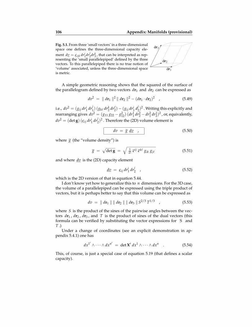
106 Appendix: Manifolds (provisional)
Fig. 5.1. From three ‘small vectors’ in a three-dimensionalspace one defines the three-dimensional capacity ele-ment dv = εijk dri
1drj2drk
3 , that can be interpreted as rep-resenting the ‘small parallelepiped’ defined by the threevectors. To this parallelepiped there is no true notion of‘volume’ associated, unless the three-dimensional spaceis metric.
dr1
dr2
dr3
A simple geometric reasoning shows that the squared of the surface ofthe parallelogram defined by two vectors dr1 and dr2 can be expressed as
dv2 = ‖ dr1 ‖2 ‖ dr2 ‖2 − (dr1 · dr2)2 , (5.49)
i.e., dv2 = (gij dri1 drj
1) (gk` drk2 dr`
2)− (gij dri1 dj
2)2 . Writing this explicitly and
rearranging gives dv2 = (g11 g22− g212) (dr1
1 dr22 − dr2
1 dr12)
2 , or, equivalently,dv2 = (det g) (εij dri
1 drj2)
2 . Therefore the (2D) volume element is
dv = g dv , (5.50)
where g (the “volume density”) is
g =√
det g =√
12! εij εk` gik gj` (5.51)
and where dv is the (2D) capacity element
dv = εij dri1 drj
2 , (5.52)
which is the 2D version of that in equation 5.44.I don’t know yet how to generalize this to n dimensions. For the 3D case,
the volume of a parallelepiped can be expressed using the triple product ofvectors, but it is perhaps better to say that this volume can be expressed as
dv = ‖ dr1 ‖ ‖ dr2 ‖ ‖ dr3 ‖ S2/3 T1/3 , (5.53)
where S is the product of the sines of the pairwise angles between the vec-tors dr1 , dr2 , dr3 , and T is the product of sines of the dual vectors (thisformula can be verified by substituting the vector expressions for S andT .)
Under a change of coordinates (see an explicit demonstration in ap-pendix 5.4.1) one has
dx1′ ∧ · · · ∧ dxn′ = det X′ dx1 ∧ · · · ∧ dxn . (5.54)
This, of course, is just a special case of equation 5.19 (that defines a scalarcapacity).

5.1 Manifolds and Coordinates 107
5.1.13 Integral (new text)
I could directly proceed here to introducing the standard integration theory,that is well developed, rigorous and. . . a little bit too abstract! The notionsbehind the current form of integration theory are clear: a coordinate systemon a manifold defines a field of forms, and the integration is introduced bydefining the exterior product of forms. But I choose here the old-fashionedapproach, where the integral appears as a limit, as I want to be sure thata non-professional mathematician understands what we are talking about,(in fact, I am quite skeptical about the ability of professional mathematiciansto tackle the real life problems we are interested in). I hope, that, while thepoint of view used here differs from the point of view on present-day math-ematical books, the resulting theory is quite general, and always equivalent—in our domain of application— to the standard theory.
There is one special point where I disagree with the current terminology:what should we call a “volume element”? It is OK in formal mathematics togive a broad meaning to this term. But we are going to be faced with twofundamentally different situations, that I need to mention now. Each pointof each of the manifolds we are going to use shall have a precise physicalinterpretation (for instance, each point may represent a particular model ofa physical system). In the first situation, we may have coordinates over themanifold (the different quantities we use to characterize the physical sys-tem), but we may not (or not yet) have introduced a notion of volume overthe manifold. For instance, can we define in a sensible way the distance be-tween two elastic media that only differ by their values of the Poisson’s ra-tio? (The answer, given in XXX [for the time being, read the footnote5] isnon-trivial). The point here is: what can we do before having agreed on theright definition of distance, and what must be postponed until some agree-ment is reached? Introducing a particular volume measure function over amanifold will always be for us a strong act. In the absence of that act, we canstill do many things, in particular, compute integrals over the manifold (us-ing arbitrary coordinates). And these computations shall, of course, have theright invariance (changing the coordinates, shall just require multiply somefunctions by the Jacobian of the transformation and divide some other func-tions by this Jacobian), so the values obtained though the integration will notdepend on the coordinates being used. To do this, to each coordinate systemwe can associate a “capacity element” (warning, mathematician would say
5 Letting σ be the Poisson’s ratio of a linearly elastic medium, the only length el-ement that has the necessary physical invariances is ds = dσ/((1 + σ)(1− 2σ)) .This can be justified on physical grounds, but also on pure mathematical grounds:it can be argued (Tarantola, 2006) that the 21-dimensional space representing allpossible elastic media is the symmetric submanifold of the Lie group manifoldGL+(6) , which a standard volume measure function (the Haar measure). Thelength element ds is just the one-dimensional restriction of this measure alongthe line corresponding to a variation of the Poisson’s ratio.

108 Appendix: Manifolds (provisional)
here “volume element”), and the relation between the two capacity elementsassociated to two coordinate systems will just be the multiplication by theright Jacobian. So, for us, a volume element will be an invariant notion, com-ing from geometrical arguments, while a capacity element will be an objectassociated to each coordinate system. Of course, a capacity element is a ca-pacity in the sense of section 5.1.4, i.e., in the terminology used by Weinberg(1972) or Winogradzki (1979), but, unfortunately, not in much use today.
Now, which kind of function can we integrate, using a capacity element,in order to obtain an invariant quantity? Certainly not a function whosevalues are invariant, but a density function (like a probability density func-tion), i.e., a function whose values are associated to the coordinate system,and which change, if we change coordinates, according to the Jacobian rule.So we will work into two quite different circumstances. Or we will handlecapacity elements and density functions, and we will need to to this using(arbitrary) coordinates, or we will handle a geometrically defined volumeelement and invariant (“volumetric”) functions. In the first case, there is nonecessity to agree on a particular notion of volume (or to privilege any par-ticular coordinate system), but we will be limited in what we can do (in theabsence of a “geometrically defined” volume element, the intersection oftwo density functions [see section 2.2] is not defined).
So, in what follows, before the formalization of the notion of integral, weshall take a finite approximation, and suggest the appropriate limit (afterwhich, the formalization shall be attempted). In fact, we shall do this twice:when we have a manifold with coordinates —but not necessarily a geomet-rical notion of volume—, and when we have a manifold with a notion ofvolume on it —but not necessarily a coordinate system—.
To intuitively help the building of the theory, we consider a particularproblem. There is some random process that generates random points of amanifold, potentially an infinite number of them. There may be many pointson some regions of the manifold, and few points on some other regions.Our goal is to make a “histogram” of the points by dividing the manifoldin finite-sized “cells” and take the limit when the size of the cells tends toinfinity. This defines a function on the manifold (the limit of the histogram)and, when given this function, we wish to evaluate the proportion of pointsinside some domain, we need to integrate the values of the function over thedomain (with the appropriate integration element). This procedure will sug-gest the proper definitions of density function and capacity element —whenworking with coordinates and no notion of volume— and the proper defi-nitions of volumetric function and volume element —when working with anotion of volume but no coordinates—.
Let us start with the first of these two possibilities, which is illustrated infigure 5.2. Consider an abstract, n-dimensional manifold M with points de-noted P, P′, . . . (in the illustration, n = 3 ). On a finite region of M we havedefined a coordinate u , i.e., a mapping P 7→ u = u(P) from the points of

5.1 Manifolds and Coordinates 109
w = 1.0
w = 1.1
w = 1.2u = 1.2
u = 1.1
u = 1.0
v = 1.2
v = 1.0
v = 1.1
Fig. 5.2. Caption be be written. For the time being, please see the text.
the manifold into the real line. This coordinate u is not assumed to have anyparticular geometrical meaning. The sets of points corresponding to con-stant values of u are (n− 1)-dimensional hypersurfaces (in the illustration,the surfaces at the left). Without the need to define other coordinates, the no-tion of histogram, of probability density, and of integral can be introduced.We consider some (finite) value ∆u , and, for some selected value u0 , weconsider the hypersurfaces . . . , u = u0, u = u0 + ∆u, u = u0 + 2∆u, . . . .When a total of K points have been randomly generated, we count howmany points there are between each pair of hypersurfaces, make a histogramof the (relative) values, as suggested at the left of figure XXX, and, if the limitwhen K → ∞ and ∆u → 0 makes sense, we obtain the probability densityf (u) suggested at the right of figure XXX. Note:
f (u) = limK→∞ , ∆u→0
k(u + ∆u, u− ∆u)2 K ∆u
. (5.55)
In turn, if f (u) is given, the proportion number of points between the hy-persurface ua and the hypersurface ub is to be evaluated as
P =∫ ub
uadu f (u) explain!. (5.56)

110 Appendix: Manifolds (provisional)
5.1.14 Integral (old text)
Consider an n-dimensional manifold M , with some coordinates xi , andassume that a scalar density f (x1, x2, . . . ) has been defined at each point ofthe manifold (this function being a density, its value at each point dependson the coordinates being used; an example of practical definition of such ascalar density is given in section 5.2.10).
Dividing each coordinate line in ‘small increments’ ∆xi divides the man-ifold M (or some domain D of it) in ‘small hyperparallelepipeds’ that arecharacterized, as we have seen, by the capacity element (equations 5.47–5.48)
∆v = ε12...n ∆x1 ∆x2 . . . ∆xn = ∆x1 ∆x2 . . . ∆xn . (5.57)
At every point, we can introduce the scalar ∆v f (x1, x2, . . . ) and, therefore,for any domain D ⊂ M , the discrete sum ∑ ∆v f (x1, x2, . . . ) can be con-sidered, where only the ‘hyperparallelepipeds’ that are inside the domainD (or at the border of the domain) are taken into account (as suggested byfigure 5.3).
Fig. 5.3. The volume of an arbitrarily shaped, smooth, domainD of a manifold M , can be defined as the limit of a sum, usingelementary regions adapted to the coordinates (regions whoseelementary capacity is well defined).
The integral of the scalar density f over the domain D is defined as thelimit (when it exists)
I =∫D
dv f (x1, x2, . . . ) ≡ lim ∑ ∆v f (x1, x2, . . . ) , (5.58)
where the limit corresponds, taking smaller and smaller ‘cells’, to consideran infinite number of them.
This defines an invariant quantity: while the capacity values ∆v and thedensity values f (x1, x2, . . . ) essentially depend on the coordinates beingused, the integral does not (the product of a capacity times a density is atensor).
This invariance is trivially checked when taking seriously the notation∫D dv f . In a change of variables x x′ , the two capacity elements dv(x)
and dv′(x′) are related via (equation 5.19)
dv′(x′) =1
X(x′)dv( x(x′) ) (5.59)

5.1 Manifolds and Coordinates 111
(where X(x′) is the Jacobian determinant det∂xi/∂xi′ ), as they are tenso-rial capacities, in the sense of section 5.1.4. Also, for a density we have
f ′(x′) = X(x′) f ( x(x′) ) . (5.60)
In the coordinates x we have
I(D) =∫
x∈Ddv(x) f (x) , (5.61)
and in the coordinates x′ ,
I(D)′ =∫
x′∈Ddv′(x′) f ′(x′) . (5.62)
using the two equations 5.59–5.60, we imediately obtain I(D) = I(D)′ thisshowing that the integral of a density (integrated using the capacity ele-ment) is an invariant.
5.1.15 Capacity Element and Change of Coordinates
Note: real text yet to be written, this is a first attempt to the demonstration.The demonstration os possibly wrong, as I have not cared to well define thenew capacity element.
At a given point of an n-dimensional manifold we can consider the nvectors dr1, . . . , drn , associated to some coordinate system x1, . . . , xn ,and we have the capacity element
dv = εi1 ...in (dr1)i1 . . . (drn)in . (5.63)
In a change of coordinates xi 7→ xi′ , each of the n vectors shall havehis components changed according to
(dr)i′ =∂xi′
∂xi (dr)i = Xi′i (dr)i . (5.64)
Reciprocally,
(dr)i =∂xi
∂xi′ (dr)i′ = Xi′i (dr)i . (5.65)
The capacity element introduced above can now be expressed as
dv = εi1 ...in Xi1i′1
. . . Xini′n (dr1)i′1 . . . (drn)i′n . (5.66)
I guess that I can insert here the factor 1n! εi′1 ...i′n εj′1 ...j′n , to obtain
dv = εi1 ...in Xi1i′1
. . . Xini′n ( 1
n! εi′1 ...i′n εj′1 ...j′n ) (dr1)j′1 . . . (drn)j′n . (5.67)

112 Appendix: Manifolds (provisional)
If yes, then I would have
dv = ( 1n! εi1 ...in εi′1 ...i′n Xi1
i′1. . . Xin
i′n ) εj′1 ...j′n (dr1)j′1 . . . (drn)j′n , (5.68)
i.e., using the definition of determinant (third of equations 5.35),
dv = det X εj′1 ...j′n (dr1)j′1 . . . (drn)j′n . (5.69)
We recognize here the capacity element dv′ = εj′1 ...j′n (dr1)j′1 . . . (drn)j′n asso-ciated to the new coordinates. Therefore, we have obtained
dv = det X dv′ . (5.70)
This, of course, is consistent with the definition of a scalar capacity (equa-tion 5.19).
5.2 Volume
5.2.1 Metric
OLD TEXT BEGINS.In some parameter spaces, there is an obvious definition of distance be-
tween points, and therefore of volume. For instance, in the 3D Euclideanspace the distance between two points is just the Euclidean distance (whichis invariant under translations and rotations). Should we choose to parame-terize the position of a point by its Cartesian coordinates x, y, z , then,
Note: I have to talk about the conmensurability of distances,
ds2 = ds2r + ds2
s , (5.71)
every time I have to define the Cartesian product of two spaces each with itsown metric.
OLD TEXT ENDS.A manifold is called a metric manifold if there is a definition of distance
between points, such that the distance ds between the point of coordinatesx = xi and the point of coordinates x + dx = xi + dxi can be expressedas6
ds2 = gij(x) dxi dxj , (5.72)
i.e., if the notion of distance is ‘of the L2 type’7. At every point of a metricmanifold, therefore, there is a symmetric tensor gij defined, the metric tensor.
6 This is a property that is valid for any coordinate system that can be chosen overthe space.
7 As a counterexample, in a two-dimensional manifold, the distance defined asds = |dx1|+ |dx2| is not of the L2 type (it is L1 ).

5.2 Volume 113
The inverse metric tensor, denoted gij , is defined by the condition
gij gjk = δik . (5.73)
It can be demonstrated that under a change of variables, its componentschange like the components of a contravariant tensor, from where the nota-tion gij . Therefore, the equations defining the change of components of themetric and of the inverse metric are (see equations 5.15)
gi′ j′ = Xii′ X j
j′ gij and gi′ j′ = X′i′i X′j′
j gij . (5.74)
In section 5.1.2, we introduced the matrices of partial derivatives. It isuseful to also introduce two metric matrices, with respectively the covariantand contravariant components of the metric:
g =
g11 g12 g13 · · ·g21 g22 g23 · · ·
......
.... . .
; g-1 =
g11 g12 g13 · · ·g21 g22 g23 · · ·
......
.... . .
, (5.75)
the notation g-1 for the second matrix being justified by the definition 5.73,that now reads
g-1 g = I . (5.76)
In matrix notation, the change of the metric matrix under a change ofvariables, as given by the two equations 5.74, is written
g′ = Xt g X ; g′-1 = X′ g-1 X′t . (5.77)
If an every point P of a manifold M there is a metric gij defined, then,the metric can be used to define a scalar product over the linear space tan-gent to M at P : given two vectors v and w , their scalar product is
v ·w ≡ gij vi wj . (5.78)
One can also define the scalar product of two forms f and h at P (formsthat belong to the dual of the linear space tangent to M at P ):
f · h ≡ gij fi hj . (5.79)
The norm of a vector v and the norm of a form f are respectively defined
as ‖ v ‖ =√
v · v =√
gij vi vj and ‖ f ‖ =√
f · f =√
gij vi vj .
5.2.2 Bijection Between Forms and Vectors
Let ei be the basis of a linear space, and ei the dual basis (that, as wehave seen, is a basis of the dual space).

114 Appendix: Manifolds (provisional)
In the absence of a metric, there is no natural association between vectorsand forms. When there is a metric, to a vector vi ei we can associate a formwhose components on the dual basis ei are
vi ≡ gij vj . (5.80)
Similarly, to a form f = fi ei , one can associate the vector whose compo-nents on the vector basis ei are
f i ≡ gij f j . (5.81)
[Note: Give here some of the properties of this association (that the scalarproduct is preserved, etc.).]
5.2.3 Kronecker Tensor (II)
The Kronecker’s tensors δij and δi
j are defined that the space has a metricor not. When one has a metric, one can raise and lower indices. Let us, forinstance, lower the first index of δi
j :
δij ≡ gik δkj = gij . (5.82)
Equivalently, let us raise one index of gij :
gij ≡ gik gkj = δi
j . (5.83)
These equations demonstrate that when there is a metric, the Kronecker tensorand the metric tensor are identical. Therefore, when there is a metric, we candrop the symbols δi
j and δij , and use the symbols gi
j and gij instead.
5.2.4 Fundamental Density
Note: I have to care here about the sign of the fundamental density. Talkwith Tolo!!! What should I take
g =√±det g or g = ±
√det g , (5.84)
or somethng else?Let g the metric tensor of the manifold. For any (positively oriented) sys-
tem of coordinates, we define the quantity g , that we call the metric density(in the given coordinates) as
g =√
det g . (5.85)
More explicitly, using the definition of determinant in the first of equa-tions 5.35,

5.2 Volume 115
g =√
1n! εi1i2 ...in εj1 j2 ...jn gi1 j1 gi2 j2 . . . gin jn . (5.86)
This equation immediately suggests what it is possible to prove: the quantityg so defined is a scalar density (at the right, we have two upper bars undera square root).
The quantityg = 1/g (5.87)
is obviously a capacity, that we call the metric capacity. It could also havebeen defined as
g =√
det g-1 =√
1n! εi1i2 ...in εj1 j2 ...jn gi1 j1 gi2 j2 . . . gin jn . (5.88)
5.2.5 Bijection Between Capacities, Tensors, and Densities
As mentioned in section 5.1.4, (i) the product of a capacity by a density isa tensor, (ii) the product of a tensor by a density is a density, and (iii) theproduct of a tensor by a capacity is a capacity. So, when there is a metric, wehave a natural bijection between capacities and tensors, and between tensorsand densities.
For instance, to a tensor capacity tij...k`... we can associate the tensor
tij...k`... ≡ g tij...
k`... (5.89)
to a tensor sij...k`... we can associate the tensor density
sij...k`... ≡ g sij...
k`... (5.90)
and the tensor capacity
sij...k`... ≡ g sij...
k`... , (5.91)
and to a tensor density rij...k`... we can associate the tensor
rij...k`... ≡ g rij...
k`... . (5.92)
Equations 5.89–5.92 introduce an important notation (that seems to be novel):in the bijections defined by the metric density and the metric capacity, wekeep the same letter for the tensors, and we just put bars or take out bars,much like in the bijection between vectors and forms defined by the metric,where we keep the same letter, and we raise or lower indices.
5.2.6 Levi-Civita Tensor
From the Levi-civita capacity εij...k we can define the Levi-Civita tensor εij...kas

116 Appendix: Manifolds (provisional)
εij...k = g εij...k . (5.93)
Explicitly, this gives
εijk... =
+√
det g if ijk . . . is an even permutation of 12 . . . n0 if some indices are identical
−√
det g if ijk . . . is an odd permutation of 12 . . . n .(5.94)
Alternatively, from the Levi-civita density εij...k we could have definedthe contravariant tensor εij...k as
εij...k = g εij...k . (5.95)
It can be shown that εij...k can be obtained from εij...k using the metric toraise the indices, so εij...k and εij...k are the same tensor (from where thenotation).
5.2.7 Volume Element
We may here start by remembering equation 5.44,
dv = εi1 ...in dri11 dri2
2 . . . drinn , (5.96)
that expresses the capacity element defined by n vectors dr1 , dr2 . . . drn .In the special situation where n vectors are taken successively along
each of the n coordinate lines, this gives (equation 5.48) dv = dx1 dx2 . . . dxn .The dxi in this expression are mere coordinate increments, that bear no re-lation to a length. As we are now working under the hypothesis that wehave a metric, we know that the length associated to the coordinate in-crement, say, dx1 , is8 ds = √
g11 dx1 . If the coordinate lines where or-thogonal at the considered point, then, the volume element, say dv , as-sociated to the capacity element dv = dx1 dx2 . . . dxn would be dv =√
g11 dx1√g22 dx2 . . .√
gnn dxn . If the coordinates are not necessarily or-thogonal, this expression needs, of course, to be generalized.
One of the major theorems of integration theory is that the actual volumeassociated to the hyperparallelepiped characterized by the capacity elementdv , as expressed by equation 5.96, is
dv = g dv , (5.97)
where g is the metric density introduced above. [Note: Should I give ademonstration of this property here?] We know that dv is a capacity, and ga density. Therefore, the volume element dv , being the product of a density
8 Because the length of a general vector with components dxi is ds2 = gij dxi dxj .

5.2 Volume 117
by a capacity is a true scalar. While dv has been called a ‘capacity element’,dv is called a volume element.
The overbar in g is to remember that the determinant of the metric ten-sor is a density, in the tensorial sense of section 5.1.4, while the underbar indv is to remember that the ‘capacity element’ is a capacity in the tensorialsense of the term. In equation 5.97, the product of a density times a capacitygives the volume element dv , that is a true scalar (i.e., a scalar whose valueis independent of the coordinates being used). In view of equation 5.97, wecan call g(x) the ‘density of volume’ in the coordinates x = x1, . . . , xn .For short, we shall call g(x) the volume density9. It is important to realizethat the values g(x) do not represent any intrinsic property of the space,but, rather, a property of the coordinates being used.
Example 5.2 In the Euclidean 3D space, using spherical coordinates x = r, θ, ϕ ,as the length element is ds2 = dr2 + r2 sin2 θ dϕ2 + r2 dθ2, the metric matrix isgrr grθ grϕ
gθr gθθ gθϕ
gϕr gϕθ gϕϕ
=
1 0 00 r2 00 0 r2 sin2 θ
. (5.98)
and the metric determinant is
g =√
det g = r2 sin θ . (5.99)
As the capacity element of the space can be expressed (using notations that are notmanifestly covariant)
dv = dr dθ dϕ , (5.100)
the expression dv = g dv gives the volume element
dv = r2 sin θ dr dθ dϕ . (5.101)
5.2.8 Volume Element and Change of Variables
Assume that one has an n-dimensional manifold M and two coordinatesystems, say x1, . . . , xn and x1′ , . . . , xn′ . If the manifold is metric, thecomponents of the metric tensor can be expressed both in the coordinatesx and in the coordinates x′ . The (unique) volume element, say dv , acceptsthe two different expressions
dv =√
det gx dx1 ∧ · · · ∧ dxn =√
det gx′ dx1′ ∧ · · · ∧ dxn′ . (5.102)
The Jacobian matrices of the transformation (matrices with the partial deriva-tives), X and X′ , have been introduced in section 5.1.3. The components ofthe metric are related through
9 So we now have two names for g , the ‘metric density’ and the ‘volume density’.
118 Appendix: Manifolds (provisional)
gi′ j′ = Xii′ X j
j′ gij , (5.103)
or, using matrix notations, gx′ = Xt gx X . Using the identities det gx′ =det(Xt gx X) = (det X)2 det gx , one arrives at√
det gx′ = det X√
det gx . (5.104)
This is he relation between the two fundamental densities associated to eachof the two coordinate systems. Of course, this corresponds to equation 5.18(page 98), used to define scalar densities.
5.2.9 Volume of a Domain
With the volume element available, we can now define the volume of a do-main D of the manifold M , that we shall denote as
V(D) =∫D
dv , (5.105)
by the expression ∫D
dv ≡∫D
dv g . (5.106)
This definition makes sense because we have already defined the integral ofa density in equation 5.58. Note that the (finite) capacity of a finite domain Dcannot be defined, as an expression like
∫D dv would make any (invariant)
sense.We have here defined equation 5.105 in terms of equation 5.106, but it
may well happen that, in numerical evaluations of an integral, the divisionof the space into small ‘hyperparallelepideds’ that is implied by the use ofthe capacity element is not the best choice. Figure 5.4 suggests a divisionof the space into ‘cells’ having grossly similar volumes (to compared withfigure 5.5). If the volume ∆vp of each cell is known, the volume of a domainD can obviously be defined as a limit
V(D) = lim∆vp→0
∑p
∆vp . (5.107)
We will discuss this point further in later chapters.The finite volume obviously satisfies the following two properties:
– for any domain D of the manifold, V(D) ≥ 0 ;– if D1 and D2 are two disjoint domains of the manifold, then V(D1 ∪
D2) = V(D1) + V(D2) .

5.2 Volume 119
Fig. 5.4. The volume of an arbitrarily shaped, smooth, domainD of a manifold M , can be defined as the limit of a sum, us-ing elementary regions whose individual volume is known(for instance, triangles in this 2D illustration). This way ofdefining the volume of a region does not require the defini-tion of a coordinate system over the space.
Fig. 5.5. For the same shape of figure 5.4, the volume can be evalu-ated using, for instance, a polar coordinate system. In a numericalintegration, regions near the origin may be oversampled, while re-gions far from the orign may be undersampled. In some situation,this problem may become crucial, so this sort of ‘coordinate inte-gration’ is to be reserved to analytical developments only.
5.2.10 Example: Mass Density and Volumetric Mass
Imagine that a large number of particles of equal mass are distributed inthe physical space (assimilated to an Euclidean 3D space) and that, for somereason, we chose to work with cylindrical coordinates r, ϕ, z . Choosingsmall increments ∆r, ∆ϕ, ∆z of the coordinates, we divide the space intocells of equal capacity, that (using notations that are not manifestly covari-ant) is given by
∆v = ∆r ∆ϕ ∆z . (5.108)
We can count how many particles are inside each cell (see figure 5.6), and,therefore which is the mass ∆m inside each cell. The quantity δm/∆v , be-ing the ratio of a scalar by a capacity is a density. In the limit of an infinitenumber of particles, we can take the limit where ∆r , ∆ϕ , and ∆z all tendto zero and the limit
ρ(r, ϕ, z) = lim∆r→0 , ∆ϕ→0 , ∆z→0
∆m∆v
(5.109)
is the mass density at point r, ϕ, z .Given the mass density ρ(r, ϕ, z) , the total mass inside a domain D of
the space is to be obtained as
M(D) =∫D
dv ρ , (5.110)
where the capacity element dv appears, not the volume element dv .If instead of dividing the space into cells of equal capacity ∆v , we divide
it into cells of equal volume, ∆v (as suggested at the right of the figure 5.6),then the limit
ρ(r, ϕ, z) = lim∆v→0
∆m∆v
(5.111)

120 Appendix: Manifolds (provisional)
ϕ ϕ
r
ϕ
.
..
..
...
..
.
..
.
.
.
...
..
..
.. .
..
.
..
.
.
..
. ..
.
.
.
.
.
.. .
..
...
. .
.
.
..
..
...
.. .
.
....
..
..
.. .
..
.
..
.
.
..
. ..
.
.
.
... .
....
.
. ..
.
..
..
...
..
.
..
.
.
.
...
..
..
.. .
..
.
..
.
.
..
. ..
.
.
.
.
.
.. .
..
...
. .
.
.
..
..
...
.. .
.
....
..
..
.. .
..
.
..
.
.
..
. ..
.
.
.
... .
....
.
. ..
....
. ...
.
.
.
.
.
..
.
..
.
.
.
.
.
.
..
.
.
.
.
.
.
..
.
.
.
.
.
.
..
..
.
.
..
.
.. .
.
.
.
.
.
.
.
.
.
..
..
...
.
.
.
.
.
.
..
..
..
.. .
.
.
..
.. .
..
.
..
.
.
..
.
.
.
...
..
.
..
Fig. 5.6. We consider, in an Euclidean 3D space, a cylinder with a circular basis ofradius 1, and cylindrical coordinates (r, ϕ, z) . Only a section of the cylinder is rep-resented in the figure, with all its thickness, ∆z , projected on the drawing plane. Atthe left, we have represented a ‘map’ of the corresponding circle, and, at the middle,the coordinate lines on a ‘metric representation’ of the space. By construction, all the‘cells’ in the middle have the same capacity ∆v = ∆r ∆ϕ ∆z . The points representparticles with given masses. As explained in the text, counting how many particlesare inside each cell directly gives an estimation of the ‘mass density’ ρ(r, ϕ, z) . Tohave, instead, a direct estimation of the ‘volumetric mass’ ρ(r, ϕ, z) , a division ofthe space into cells of equal volume (not equal capacity) should have been done, assuggested at the right.
gives the volumetric mass ρ(r, ϕ, z) , different from the mass density ρ(r, ϕ, z) .Given the volumetric mass density ρ(r, ϕ, z) , the total mass inside a domainD of the space is to be obtained as
M(D) =∫D
dv ρ , (5.112)
where the volume element dv appears, not the capacity element dv . Therelation between the mass density ρ and the volumetric mass ρ is the uni-versal relation between any scalar density and a scalar,
ρ = g ρ , (5.113)
where g is the metric density. As in cylindrical coordinates, g = r , therelation between mass density and volumetric mass is
ρ(r, ϕ, z) = r ρ(r, ϕ, z) . (5.114)
It is unfortunate that in common physical terminology the terms ‘massdensity’ and ‘volumetric mass’ are used as synonymous. While for commonapplications, this does not pose any problem, there is a sometimes a seriousmisunderstanding in probability theory about the meaning of a ‘probabilitydensity’ and of a ‘volumetric probability’.

5.3 Mappings 121
5.3 Mappings
Note: explain here that we consider a mapping from a p-dimensional mani-fold M into a q-dimensional manifold N .
5.3.1 Image of the Volume Element
This section is very provisional. I do not know yet how much of it I willneed.
We have p-dimensional manifold, with coordinates xa = x1, . . . , xp .At a given point, we have p vectors dx1, . . . , dxp . The associated capacityelement is
dv = εa1 ...ap (dx1)a1 . . . (dxp)ap . (5.115)
We also have a second, q-dimensional manifold, with coordinates ψα =ψ1, . . . , ψq . At a given point, we have q vectors dψ1, . . . , dψq . The as-sociated capacity element is
dω = εα1 ...αq (dψ1)α1 . . . (dψq)
αq . (5.116)
Consider now an application
x 7→ ψ = ψ(x) (5.117)
from the first into the second manifold. I examine here the case
p ≤ q , (5.118)
i.e., the case where the dimension of the first manifold is smaller or equalthan that of the second manifold. When transporting the p vectors dx1, . . . , dxpfrom the first into the second manifold (via the application ψ(x) ), this willdefine on the q-dimensional manifold a p-dimensional capacity element,dωp . We wish to relate dωp and dv .
It is shown in the appendix (check!) that one has
dωp =√
det(Ψt Ψ) dv . (5.119)
Let us be interested in the image of the volume element. We denote byg the metric tensor of the first manifold, and by γ the metric tensor of thesecond manifold.
Bla, bla, bla, and it follows from this that when letting dωp be the (p-dimensional) volume element obtained in the (q-dimensional) second man-ifold by transport of the volume element dv of the first manifold, one has
dωp
dv=
√det(Ψt γ Ψ)√
det g. (5.120)

122 Appendix: Manifolds (provisional)
5.3.2 Reciprocal Image of the Volume Element
I do not know yet if I will need this section.
5.4 Appendices for Manifolds (check)
5.4.1 Capacity Element and Change of Coordinates
Consider the problem, when dealing with an n-dimensional manifold, topass from a coordinate system xα = x1, . . . , xn to some other coordi-nate system xα′ = x1′ , . . . , xn′ , and let be, as usual,
Xαα′ =
∂xα
∂xα′; Xα′
α =∂xα′
∂xα. (5.121)
The capacity elements in each of the two coordinate systems are
dv = εα1 ...αn dxα1 . . . dxαn ; dv′ = εα′1 ...α′n dxα′1 . . . dxα′n , (5.122)
and one can write
dv′ = εα′1 ...α′n Xα′1 α1 . . . Xα′n αn dxα1 . . . dxαn . (5.123)
Because of the antisymmetry properties of the Levi-Civita densities and ca-pacities, this can also be written (see relations 5.34) as
dv′ = εα′1 ...α′n Xα′1 β1 . . . Xα′nβn ( 1
n! εβ1 ...βn εα1 ...αn ) dxα1 . . . dxαn , (5.124)
i.e.,
dv′ = ( 1n! εα′1 ...α′n Xα′1 β1 . . . Xα′n
βn εβ1 ...βn ) εα1 ...αn dxα1 . . . dxαn , (5.125)
In the left-hand side, onr recognizes the definition of a determinant (see thethird of equations 5.35) and one finds the capacity element dv introducedabove, so one finally has
dv′ = (det X′) dv , (5.126)
as one should, as this is the general expression for the change of value of ascalar10 capacity.
10 A scalar capacity is a capacity of rank (or order) zero, i.e., a capacity “having notensor indices”.

5.4 Appendices for Manifolds (check) 123
5.4.2 Conditional Volume
Consider an n-dimensional manifold Mn , with some coordinates x1, . . . , xn ,and a metric tensor gij(x) . Consider also a p-dimensional submanifold Mpof the n-dimensional manifold Mn (with p ≤ n ). The n-dimensional vol-ume over Mn , as characterized by the metric determinant g =
√det g ,
induces a p-dimensional volume over the submanifold Mp . Let us try tocharacterize it.
The simplest way to represent a p-dimensional submanifold Mp ofthe n-dimensional manifold Mn is by separating the n coordinates x =x1, . . . , xn of Mn into one group of p coordinates r = r1, . . . , rp andone group of q coordinates s = s1, . . . , sq , with
p + q = n . (5.127)
Using the notations
x = x1, . . . , xn = r1, . . . , rp, s1, . . . , sq = r, s , (5.128)
the set of q relations
s1 = s1(r1, r2, . . . , rp)s2 = s2(r1, r2, . . . , rp)
. . . = . . .sq = sq(r1, r2, . . . , rp) , (5.129)
that, for short, may be written
s = s(r) , (5.130)
define a p-dimensional submanifold Mp in the (p + q)-dimensional mani-fold Mn . For later use, we can now introduce the matrix of partial deriva-tives
S =
S1
1 S12 · · · S1
pS2
1 S22 · · · S2
p...
.... . .
...Sq
1 Sq2 · · · Sq
p
=
∂s1
∂r1∂s1
∂r2 · · · ∂s1
∂rp
∂s2
∂r1∂s2
∂r2 · · · ∂s2
∂rp
......
. . ....
∂sq∂r1
∂sq∂r2 · · ·
∂sq∂rp
. (5.131)
We can write S(r) for this matrix, as it is defined at a point x = r, s(r) .Note also that the metric over Mn can always be partitioned as
g(x) = g(r, s) =(
grr(r, s) grs(r, s)gsr(r, s) gss(r, s)
), (5.132)
with grs = (gsr)T .

124 Appendix: Manifolds (provisional)
r2
s
r1
s
r1
s = s( r , r )1 2
Some surface coordinates
of a coordinate system
over a 3D manifold
An elementary region
on the coordinate surface
defined by a condition
s = constant
An elementary region
on the surface
defined by a condition
dSdSr
2
s = s( r , r )1 2
Fig. 5.7. On a 3D manifold, a coordinate system x1, x2, x3 = r1, r2, s is defined.Some characteristic surface coordinates are represented (left). In the middle, a surfaceelement (2D volume element) on a coordinate surface s = const. is represented,that corresponds to the expression in equation 5.133. In the right, a submanifold(surface) is defined by an equation s = s(r1, r2) . A surface element (2D volumeelement) is represented on the submanifold, that corresponds to the expression inequation 5.134.
In what follows, let us use the Greek indexes α, β . . . r1, . . . , rp , likein rα ; α ∈ 1, . . . , p , and the Latin indexes a, b . . . for the variabless1, . . . , sq , like in sa ; a ∈ 1, . . . , q . Consider an arbitrary point r, s ofthe manifold M . If the coordinates rα are perturbed to rα + drα , with thecoordinates sa kept unperturbed, one defines a p-dimensional submanifoldof the n-dimensional manifold Mn . The volume element of this submani-fold can be written (middle panel in figure 5.7)
dvp(r, s) =√
det grr(r, s) dr1 ∧ · · · ∧ drp . (5.133)
Alternatively, consider a point (r, s) of Mn that, in fact, is on the sub-manifold Mp , i.e., a point that has coordinates of the form (r, s(r)) . It isclear that the variables r1 . . . rp define a coordinate system over the sub-manifold, as it is enough to precise r to define a point in Mp . If the co-ordinates rα are perturbed to rα + drα , and the coordinates sa are alsoperturbed to sa + dsa in a way that one remains on the submanifold, (i.e.,with dsa = Sa
α drα ), then, with the metric over Mn partitioned as inequation 5.132, the general distance element ds2 = gij dxi dxj can be writ-ten ds2 = (grr)αβ drα drβ + (grs)αb drα dsb + (gsr)aβ dsa drβ + (gss)ab dsa dsb ,and replacing dsa by dsa = Sa
α drα , we obtain ds2 = Gαβ drα drβ , withG = grr + grs S + ST gsr + ST gss S . The ds2 just expressed gives the dis-tance between two any points of Mp , i.e., G is the metric matrix of thesubmanifold associated to the coordinates r .
The p-dimensional volume element on the submanifold Mp is, then,dvr =
√det G dr1 ∧ · · · ∧ drp , i.e.,
5.4 Appendices for Manifolds (check) 125
dvp(r) =√
det (grr + grs S + ST gsr + ST gss S) dr1 ∧ · · · ∧ drp ,
(5.134)where, if the variables are explicitly written, S = S(r) , grr = grr(r, s(r)) ,grs = grs(r, s(r)) , gsr = gsr(r, s(r)) and gss = gss(r, s(r)) . Figure 5.7 illus-trates this result. The expression 5.134 says that the p-dimensional volumedensity induced over the submanifold Mp is
gp =√
det (grr + grs S + ST gsr + ST gss S) . (5.135)
Note that the notion of ‘conditional volume’ just explored does not makeany sense when the manifold is not metric.


6 Appendix: Marginal and ConditionalProbabilities (very provisional)
6.1 Conditional Probability Function
6.1.1 Conditional Probability (provisional text I)
When one has a probability function P defined over some set Ω one some-times needs to introduce another probability function over Ω , similar to theinitial P , but that now gives zero probability to any set outside some givenset C . This is achieved by introducing the following definition.
Definition 6.1 Conditional probability. Let P be a probability function oversome set Ω , and let C ⊆ Ω be some subset with non-zero probability, P[C] > 0 .The conditional probability of any set A ⊆ Ω “given the set C ” is denotedP[A|C] , and is defined as
P[A|C] =P[A∩C]
P[C]. (6.1)
The set C is called the conditioning set.
It is clear that, as intended, the probability of any set A such that A∩C = ∅is zero. Let us verify that the mapping A 7→ P[A|C] is, indeed, a probabilitymapping. First, it is obvious that P[ ∅ |C] = 0 and that P[Ω|C] = 1 . Sec-ond, it is easy to verify1 that one has P[A1 ∪A2|C] = (P[A1|C] + P[A2|C]−P[A1 ∩A2|C]) , so the basic axiom of a measure is also satisfied. A specialcase of conditional probability is introduced in example 6.16.
Example 6.1 When working with a discrete set, introducing the elementary con-ditional probability p(ω|C) via
P[A|C] = ∑ω∈A
p(ω|C) , (6.2)
one finds
1 One can successively write P[A1 ∪A2|C] = P[(A1 ∪A2)∩C]/P[C] =P[(A1 ∩C)∪ (A2 ∩C)]/P[C] = (P[A1 ∩C] + P[A2 ∩C] −P[(A1 ∩C)∩ (A2 ∩C)])/P[C] = (P[A1 ∩C] + P[A2 ∩C] −P[(A1 ∩A2)∩C])/P[C] = (P[A1|C] + P[A2|C]− P[A1 ∩A2|C]) .

128 Appendix: Marginal and Conditional Probabilities (very provisional)
p(ω|C) =
p(ω) / ∑ω′∈C p(ω′) if ω ∈ C
0 if ω /∈ C .(6.3)
Given a probability function P , and given two sets A1 and A2 withnonzero probability, one may introduce the two conditional probabilitiesP[A1|A2] = P[A1 ∩ A2]/P[A2] and P[A2|A1] = P[A2 ∩A1]/P[A1] . AsA2 ∩A1 = A1 ∩A2 , these two expressions, taken together, imply the re-lation
P[A2|A1] =P[A1|A2] P[A2]
P[A1], (6.4)
well-known under the name of Bayes theorem. This relation is the startingpoint to many approaches intended to solve “inference problems”. In thistext, I rather choose to use the notions of intersection of two probabilities, ofimage of a probability, and of reciprocal image of a probability, so the Bayestheorem, will not by of any use to us.
6.1.2 Conditional Probability (provisional text II)
As in section 5.4.2, consider an n-dimensional manifold Mn , with some co-ordinates x = x1, . . . , xn , and a metric tensor g(x) = gij(x) . The n-dimensional volume element is, then, dV(x) = g(x) dv(x) =
√det g(x) dx1∧
· · · ∧ dxn . In section 5.4.2, the n coordinates x = x1, . . . , xn of M havebeen separated into one group of p coordinates r = r1, . . . , rp and onegroup of q coordinates s = s1, . . . , sq , with p + q = n , and a p-dimensional submanifold Mp of the n-dimensional manifold M (withp ≤ n ) has been introduced via the constraint
s = s(r) . (6.5)
Consider a probability distribution P over Mn , represented by the vol-umetric probability f (x) = f (r, s) . We wish to define (and to characterize)the ‘conditional volumetric probability’ induced over the submanifold bythe volumetric probability f (x) = f (r, s) .
Given the p-dimensional submanifold Mp of the n-dimensional mani-fold Mn , one can define a set B(∆s) as being the set of all points whose dis-tance to the submanifold Mp is less or equal than ∆s . For any finite valueof ∆s , Kolmogorov’s definition of conditional probability applies, and theconditional probability so defined associates, to any D ⊂ Mn , the prob-ability ??. Excepted for a normalization factor, this conditional probabilityequals the original one, excepted in that all the domain whose points are ata distance larger than ∆s have been ‘trimmed away’. This is still a prob-ability distribution over Mn . In the limit when ∆s → 0 this shall definea probability distribution over the submanifold Mp that we are about tocharacterize.

6.1 Conditional Probability Function 129
Consider a volume element dvp over the submanifold Mn , and all thepoints of Mn that are at a distance smaller or equal that ∆s of the pointsinside the volume element. For small enough ∆s the n-dimensional volume∆vn so defined is
∆vn ≈ dvp ∆ωq , (6.6)
where ∆ωq is the volume of the q-dimensional sphere of radius ∆s thatis orthogonal to the submanifold at the considered point. This volume isproportional to (∆s)q , so we have
∆vn ≈ k dvp (∆s)q , (6.7)
where k is a numerical factor. The conditional probability associated of thisn-dimensional domain by formula ?? is, by definition of volumetric proba-bility,
dP(p+q) ≈ k′ f ∆vn ≈ k′′ f dvp (∆s)q , (6.8)
where k′ and k′′ are constants. The conditional probability of the p-dimensionalvolume element dvp of the submanifold Mp is then defined as the limit
dPp = lim∆s→0
dP(p+q)
(∆s)q , (6.9)
this giving dPn = k′′ f dvp , or, to put the variables explicitly,
dPn(r) = k′′ f (r, s(r)) dvp(r) . (6.10)
We have thus arrived at a p-dimensional volumetric probability over thesubmanifold Mp that is given by
fp(r) = k′′ f (r, s(r)) , (6.11)
where k′′ is a constant. If the probability is normalizable, and we choose tonormalize it to one, then,
fp(r) =f (r, s(r))∫
r∈Mpdvp(r) f (r, s(r))
. (6.12)
With this volumetric probability, the probability of a domain Dp of the sub-manifold is computed as
P(Dp) =∫
r∈Dpdvp(x) fp(r) . (6.13)

130 Appendix: Marginal and Conditional Probabilities (very provisional)
6.1.3 Conditional Probability (provisional text III)
Note to the reader: this section can be skipped, unless one is particularlyinterested in probability densities.
In view of equation 6.56, the conditional probability density (over the sub-manifold Mp ) is to be defined as
f p(r) = gp(r) fp(r) (6.14)
i.e.,f p(r) = ηr
√det gp(r) fp(r) , (6.15)
so the probability of a domain Dp of the submanifold is given by
P(Dp) =∫
r∈Mpdvp(r) f p(r) , (6.16)
where dvp(r) = dr1 ∧ · · · ∧ drp .We must now express f p(r) in terms of f (r, s) . First, from equations 6.51
and 6.15 we obtain
f p(r) = ηr
√det gp(r)
f (r, s(r))∫r∈Mp
dvp(r) f (r, s(r)). (6.17)
As f (r, s) = f (r, s)/(η√
det g ) (equation ??),
f p(r) = ηr
√det gp(r)
f (r, s(r))/√
det g∫r∈Mp
dvp(r) f (r, s(r))/√
det g. (6.18)
Finally, using 6.53, and expliciting gp(r) ,
f p(r) =
√det(grr+grs S+ST gsr+ST gss S)√
det gf (r, s(r))∫
r∈Mpdr1 ∧ · · · ∧ drp
√det(grr+grs S+ST gsr+ST gss S)√
det gf (r, s(r))
.
(6.19)Again, it is understood here that all the ‘matrices’ are taken at the point( r, s(r) ) .
This expression does not coincide the the conditional probability definedgiven in usual texts (even when the manifold is defined by the conditions = s0 = const. ). This is because we contemplate here the ‘metric’ or ‘or-thogonal’ limit to the manifold (in the sense of figure ??), while usual textsjust consider the ‘vertical limit’. Of course, I take this approach here becauseI think it is essential for consistent applications of the notion of conditionalprobability. The best known expression of this problem is the so called ‘BorelParadox’ that we analyze in section 6.5.

6.1 Conditional Probability Function 131
Example 6.2 If we face the case where the space M is the Cartesian product oftwo spaces R×S , with guv = gvu = 0 , grr = gr(r) and gss = gs(s) , thendet g(r, s) = det gr(r) det gs(s) , and the conditional probability density of equa-tion 6.19 becomes,
f p(r) =
√det(gr(r)+ST(r) gs(s(r)) S(r))√
det gr(r)√
det gs(s(r))f (r, s(r))∫
r∈Mpdr1 ∧ · · · ∧ drp
√det(gr(r)+ST(r) gs(s(r)) S(r))√
det gr(r)√
det gs(s(r))f (r, s(r))
.
(6.20)
Example 6.3 If, in addition to the condition of the previous example, the hyperfur-face is defined by a constant value of s , say s = s0 , then, the probability densitybecomes
f p(r) =f (r, s0)∫
r∈Mpdr1 ∧ · · · ∧ drp f (r, s0)
. (6.21)
Example 6.4 In the situation of the previous example, let us rewrite equation 6.21dropping the index 0 from s0 , and use the notations
f r|s(r|s) =f (r, s)f s(s)
, ; f s(s) =∫
r∈Mpdr1 ∧ · · · ∧ drp f (r, s) .
(6.22)We could redo all the computations to define the conditional for s , given a fixedvalue v , but it is clear by simple analogy that we obtain, in this case,
f s|r(s|r) =f (r, s)f r(r)
, ; f r(r) =∫
r∈Mqds1 ∧ · · · ∧ dsq f (r, s) .
(6.23)Solving in these two equations for f (r, s) gives the ‘Bayes theorem’
f s|r(s|r) =f r|s(r|s) f s(s)
f r(r). (6.24)
Note that this theorem is valid only if we work in the Cartesian product of twospaces. In particular, we must have gss(r, s) = gs(s) . Working, for instance, atthe surface of the sphere with geographical coordinates (r, s) = (r, s) = (ϕ, λ)this condition is not fulfilled, as gϕ = cos λ is a function of λ : the surface ofthe sphere is not the Cartesian product of two 1D spaces. A we shall later see, thisenters in the discussion of the so-called ‘Borel paradox’ (there is no paradox, if wedo things properly).
6.1.4 Conditional Probability (provisional text IV)
Note: explain here that a condition is a subset.

132 Appendix: Marginal and Conditional Probabilities (very provisional)
– Example: a ≥ 3 . ( P( a | a ≥ 3 ) )– Example: b = a2 . ( P( a, b | b = a2 ) )– Example: b 6= a2 . ( P( a, b | b 6= a2 ) )
Consider a probability P over a set A0 , and a given set C ⊆ A0 ofnonzero probability (i.e, such that with P[C] 6= 0 ). The set C is called “thecondition”. The conditional probability (with respect to the condition C ) is,by definition, the probability (over A0 ) that to any A ⊆ A0 associates thenumber, denoted P[ A |C ] , defined as
P[ A |C ] =P[ A∩C ]
P[C]. (6.25)
This number is called “the conditional probability of A given (the condi-tion) C ”.
This, of course, is the original Kolmogorov’s definition of conditionalprobability, so, to demonstrate that this defines, indeed, a probability, wecan just outline here the original demonstration. (Note: do it!)
Example 6.5 A probability P over a discrete set A0 with elements a, a′ . . . isrepresented by the elementary probability p defined, as usual, a p(a) = P[a] .Then, the probability of any set A ⊆ A0 is P[A] = ∑a∈A p(a) . Given, now, aset C ⊆ A0 , the elementary probability that represents the probability P[ · |C ] ,denoted p( · |C ) , is given (for any a ∈ A0 ) by
p( a |C ) =
p(a) / ν if a ∈ C
0 if a /∈ C ,(6.26)
where ν is the normalizing constant ν = ∑a∈C p(a) . Then, for any A ⊆ A0 ,P[ A |C ] = ∑a∈A p( a |C ) .
Example 6.6 Let us consider a probability over NNN×NNN . By definition, then, eachelement a ∈ NNN×NNN is an ordered pair of natural numbers, that we may denotea = n, m . To any probability P over NNN×NNN is associated a nonnegative realfunction p(n, m) defined as
p(n, m) = P[n, m] . (6.27)
Then, for any A ⊆NNN×NNN
P[A] = ∑n,m∈A
p(n, m) . (6.28)
As suggested above, we call p(n, m) the elementary probability of the elementn, m . While P associates a number to every subset of NNN ×NNN , p associatesa number to every element of NNN×NNN . (Note: I have already introduced this notionabove; say where.) Introduce now the condition m = 3 . This corresponds to the

6.1 Conditional Probability Function 133
subset C of NNN×NNN made by all pairs of numbers of the form n, 3 . If P is suchthat P[C] 6= 0 , we can introduce the conditional probability P[ · |C ] . To this con-ditional probability is associated an elementary probability q(n, m) , that that wemay also denote p( n, m |m = 3 ) . It can be expressed as
q(n, m) = p( n, m |m = 3 ) =
p(n, m) / ∑n∈NNN p(n, m) if m = 3
0 if m 6= 3 .(6.29)
Note that, although the elementary probability q(n, m) takes only nonzero valueswhen m = 3 , it is a probability over NNN×NNN , not a probability over NNN .
The definition of conditional probability applies equally well when wedeal with discrete probabilities or when we deal with manifolds. But whenworking with manifolds, there is one particular circumstance that needsclarification: when instead of conditioning the original probability by a sub-set of points that has (as a manifold) the same dimensions as the originalmanifold, we consider a submanifold with lower number of dimensions. Asthis situation shall have a tremendous practical importance (when dealingwith the so-called inverse problems), let us examine it here.
Consider a manifold M with m dimensions, and let C be a (strict) sub-manifold of M . Denoting my c the number of dimensions of C , then, byhypothesis, c < m . Consider now a probability P defined over M . Asusual, P[A] then denotes the probability of any set of points A ⊆ M . Canwe define P[ A |C ] , the conditional probability over M given the (condi-tion represented by the) submanifold C ? The answer is negative (unlesssome extra ingredient is added). Let us see this.
(Note: explain here that we need to take a “uniform limit”, and, for that,we need a metric manifold.)
Example 6.7 Let M be a finite-dimensional manifold, with points respectively de-noted P, P′ . . . , and let C be a submanifold of M , i.e., a manifold contained in Mand having a smaller number of dimensions. Let now P denote a probability func-tion over M : to any set A ⊆ M it associates the (unconditional) probability valueP[ A ] . How can we characterize the conditional probability function P[ · |C ] thatto any set A ⊆ M associates the probability value P[ A |C ] ? This can be done byconsidering some set C ⊆ M (having the same dimension than M , and taking anuniform limit C → C . Such a limit can only be taken if the manifold M is metric(note: explain why). This has two implications. First, there is a volume element overM , that we may denote dvM , and, therefore, the unconditional probability P canbe represented by a volumetric probability f (P) , such that, for any A ⊆ M ,
P[ A ] =∫P∈A
dvM f ( P ) . (6.30)
The second implication is that a metric over the manifold M induces a metric overany submanifold of M . Therefore, there will also be a volume element dvC over

134 Appendix: Marginal and Conditional Probabilities (very provisional)
C (whose expression we postpone to example 6.8). Given this volume element, wecan introduce the conditional volumetric probability over C , that we may denotef ( P |N ) . By definition, then, for any set B ⊆ C ,
P[ B |C ] =∫P∈B
dvC f ( P |C ) . (6.31)
It turns out (note: refer here to the demonstration in the appendixes) that (at everypoint P of C ) the conditional volumetric probability equals the unconditional one:
f ( P |C ) = f ( P ) . (6.32)
This result is not very surprising, as we have introduced volumetric probabilitiesto have this kind of simple results (that would not hold if working with probabilitydensities). It remains, in this example, that the most important problem —to expressthe induced volume element dvC — is not solved (it is solved below).
Example 6.8 Let M and N two finite-dimensional manifolds, with points respec-tively denoted P, P′ . . . and Q, Q′ . . . , and let ϕ be a mapping from M into N .We can represent this mapping as P 7→ Q = ϕ(P) . The points P, Q of themanifold M×N that satisfy Q = ϕ(P) , i.e., the points of the form P , ϕ(P) ,constitute a submanifold, say C , of M×N . The dimension of C equals the dimen-sion of M . Consider now a probability P over M×N . By definition, the (uncon-ditional) probability value of any set A ⊆ M×N is P[A] . Which is the condi-tional probability P[ A | Q = ϕ(P) ] ? Again, one starts by introducing some setC ⊆ M×N , and tries to define the conditional probability function by taking anuniform limit C → C . To define an uniform limit, we need a metric over M×N .Typically, one has a metric over M , with distance element ds2
M , and a metricover N , with distance element ds2
N , and one defines ds2M×N = ds2
M + ds2N . Let
gM denote the metric tensor over M and let gN denote the metric tensor over N .Then, the metric tensor over M×N is gM×N = gM⊗ gN , and as demonstratedin appendix XXX, the metric tensor induced over C is
gC = gM + Φt gN Φ , (6.33)
where Φ denotes the (linear) tangent mapping to the mapping ϕ (at the consideredpoint), and where Φt is the transpose of this linear mapping. We then have (i) avolume element dvM over M (remember that a choice of coordinates over a metricmanifold induces a capacity element dv , and that the volume element can then beexpressed as dv = g dv , with g =
√det g ), (ii) a volume element dvN over
N , (iii) a volume element dvM×N = dvM dvN (note: check this!) over M×N ,and (iv) a volume element dvC over C (the volume element associated to the metricgiven in equation 6.33). We can now come back to the original (unconditional) prob-ability P[ · ] defined over M×N . Associated to it is the (unconditional) volumet-ric probability f (P, Q) , and, by definition, the probability of any set A ⊆ M×Nis
P[ A ] =∫P,Q∈A
dvM×N f (P, Q) . (6.34)

6.1 Conditional Probability Function 135
The conditional volumetric probability f ( P , Q | Q = ϕ(P) ) , associated to theconditional probability function P[ · | Q = ϕ(P) ] is, by definition, such that theconditional probability of any set B ⊆ C is obtained as
P[ B | Q = ϕ(P) ] =∫P,Q∈B
dvC f ( P , Q | Q = ϕ(P) ) . (6.35)
But, for the reason explained in the previous example, for any point (on C ),f ( P , Q | Q = ϕ(P) ) = f (P, Q) , so, for any set B ⊆ C ,
P[ B | Q = ϕ(P) ] =∫P,Q∈B
dvC f (P, Q) . (6.36)
There are two differences between the sums at the right in expressions 6.34 and 6.36:(i) the first sum is over a subset of the the manifold M×N , while the second sumis over a subset of the submanifold C ; and (ii) in the first sum, the volume elementis the original volume element over M × N , while in the second sum, it is thevolume element over C that is associated to the induced metric gC (expressed inequation 6.33). (Note: Say here that the expression of this volume element whensome coordinates are chosen over the manifolds, is given elsewhere in this text.)
Note: In the next section, the marginal of the conditional is defined. Us-ing the formulas obtained elsewhere in this text (see section ??), we obtainthe result —for the marginal of the conditional— that the probability of anyset M ⊆ M is
PM[ M | Q = ϕ(P) ] =1ν
∫P∈M
dvM ω(P) f ( P , ϕ(P) ) , (6.37)
whereω(P) =
√det( gM + Φt gN Φ ) , (6.38)
and where ν is a normalization constant. In a typical “inverse problem” onehas
f (P, Q) = g(P) h(Q) , (6.39)
and equation 6.37 becomes
PM[ M | Q = ϕ(P) ] =1ν
∫P∈M
dvM ω(P) g(P) h( ϕ(P) ) . (6.40)
While the “prior” volumetric probability is g(P) , we see that the “poste-rior” volumetric probability is
i(P) =1ν
g(P) L(P) , (6.41)
where the “likelihood volumetric probability” L(P) is
L(P) = ω(P) h( ϕ(P) ) . (6.42)
Note that we have the factor ω(P) that is not there when, instead of the“marginal of the conditional” approach, we follow the “mapping of proba-bilities” approach.
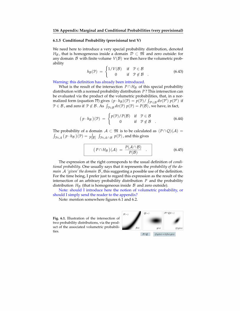
136 Appendix: Marginal and Conditional Probabilities (very provisional)
6.1.5 Conditional Probability (provisional text V)
We need here to introduce a very special probability distribution, denotedHB , that is homogeneous inside a domain D ⊂ M and zero outside: forany domain B with finite volume V(B) we then have the volumetric prob-ability
hB(P) =
1/V(B) if P ∈ B
0 if P 6∈ B .(6.43)
Warning: this definition has already been introduced.What is the result of the intersection P∩HB of this special probability
distribution with a normed probability distribution P ? This intersection canbe evaluated via the product of the volumetric probabilities, that, in a nor-malized form (equation ??) gives (p · hB)(P) = p(P)/
∫P′∈B dv(P′) p(P′) if
P ∈ B , and zero if P 6∈ B . As∫P∈B dv(P) p(P) = P(B) , we have, in fact,
(p · hB
)(P) =
p(P)/P(B) if P ∈ B
0 if P 6∈ B .(6.44)
The probability of a domain A ⊂ M is to be calculated as (P∩Q)(A) =∫P∈A
(p · hB
)(P) = 1
P(B)
∫P∈A∩B p(P) , and this gives
(P∩HB
)(A) =
P(A∩B)P(B)
. (6.45)
The expression at the right corresponds to the usual definition of condi-tional probability. One usually says that it represents the probability of the do-main A ‘given’ the domain B , this suggesting a possible use of the definition.For the time being, I prefer just to regard this expression as the result of theintersection of an arbitrary probability distribution P and the probabilitydistribution HB (that is homogeneous inside B and zero outside).
Note: should I introduce here the notion of volumetric probability, orshould I simply send the reader to the appendix?
Note: mention somewhere figures 6.1 and 6.2.
Fig. 6.1. Illustration of the intersection oftwo probability distributions, via the prod-uct of the associated volumetric probabili-ties.
P( ).
f(x)
Q( )
g(x)
.(P∩Q)( )
(f g)(x) = k f(x) g(x)
(f g)(x)
P∩Q
.
.

6.1 Conditional Probability Function 137
Fig. 6.2. Illustration of the definition of con-ditional probability. Given an intial prob-ability distribution P( · ) (left of the fig-ure) and a set B (middle of the figure),P( · |B) is identical to P( · ) inside B (ex-cept for a renormalization factor guarantee-ing that P(B|B) = 1 ) and vanishes outsideB (right of the figure)
B
H(x)
P( ).
p(x)
P( |B).
p(x|B)
P(A∩B)
P(B)P(A|B) = p(x|B) = k p(x) H(x)
6.1.6 Conditional Probability (provisional text VI)
Assume that there is a probability distribution defined over an n-dimensionalmetric manifold Mn . This probability distribution is represented by the vol-umetric probability fn(P) . Inside the manifold Mn we consider a subman-ifold Mp with dimension p ≤ n . Which is the probability distribution in-duced over Mp ? This situation, schematized in figure 6.3, has a well definedsolution because we assume that the initial manifold Mn is metric2.
Fig. 6.3. In an n-dimensional metric manifold Mn , some ran-dom points suggest a probability distribution. On this mani-fold, there is a submanifold Mp , and we wish to evaluate theprobability distribution over Mp induced by the probabilitydistribution over Mn .
.
.
.
.
.
..
.
.
.
.
.
.
.
.
.
.
.
.
.
.
.
.
.
.
.
.
.
.
.
.
.
.
.
.
.
.
.
.
.
.
.
.
.
.
.
.
.
.
.
.
.
.
.
.
.
.
.
.
.
.
.
.
..
.
.
.
.
.
.
.
.
.
.
.
.
.
.
.
.
.
.
.
.
.
.
.
.
.
.
.
.
.
.
.
.
.
.
.
.
.
.
.
.
.
.
.
.
.
.
.
.
.
.
.
.
.
.
.
.
..
.
.
.
.
.
.
.
.
.
.
.
..
.
.
.
.
.
.
.
.
.
.
.
.
.
.
.
.
.
.
.
.
.
.
.
.
.
.
.
.
.
.
.
.
.
.
.
.
.
.
.
.
.
.
.
.
.
.
.
.
.
.
.
.
.
.
.
. .
.
.
.
..
.
.
. ..
.
.
..
.
.
.
.
.
.
.
.
.
.
.
.
.
.
.
...
.
.
.
.
.
.
.
.
.
.
.
.
.
.
.
.
.
.
.
.
.
.
.
.
.
.
.
.
.
.
.
.
.
.
.
. .
.
.
.
.
.
.
.
.
.
.
.
.
.
.
.
.
.
.
.
.
.
.
.
.
.
.
.
.
.
.
.
.
Mn
Mp
The careful, quantitative, analysis of this situation is done in appendix 6.1.2.The result obtained is quite simple, and could have been guessed. Let us ex-plain it here with some detail.
The initial volumetric probability (over Mn ) is fn(P) , that me may as-sume to be normalized to one. The probability of a domain Dn ⊂ Mn isevaluated via
P(Dn) =∫P∈Dn
dvn(P) fn(P) . (6.46)
It happens (see appendix 6.1.2) that the induced volumetric probability overMp has the value
fp(P) =fn(P)∫
P′∈Dpdvp(P′) fp(P′)
(6.47)
2 Therefore, we can consider a ‘bar’ of constant ‘thickness’ around Mp and takethe limit where the thickness tends uniformly to zero. All this can be done with-out using any special coordinate system, so we obtain an invariant result. If themanifold is not metric, there is no way to define a uniform limit.

138 Appendix: Marginal and Conditional Probabilities (very provisional)
at any point P ∈ Mp (and is undefined at any point P 6∈ Mp ). So, onthe submamifold Mp , the induced volumetric probability fp(P) takes thesame values than the original volumetric probability fn(P) , excepted fora renormalization factor. The probability of a domain Dp ⊂ Mp is to beevaluated as
P(Dp) =∫P∈Dp
dvp(P) fp(P) . (6.48)
Example 6.9 In the Euclidean 3D space, consider an isotropic Gaussian probabil-ity distribution with standard deviation σ . Which is the conditional (2D) volumet-ric probability it induces on the surface of a sphere of unit radius whose center is atunit distance from the center of the Gaussian? Using geographical coordinates (seefigure 6.4), the answer is given by the (2D) volumetric probability
f (ϕ, λ) = k exp(
sin λ
σ2
), (6.49)
where k is a norming constant (demonstration in section 9.6.6). This is the cele-brated Fisher probability distribution, widely used as a model probability on thesphere’s surface. The surface element over the surface of the sphere could be obtainedusing the equations 6.54–6.55, but it is well known to be dS(ϕ, λ) = cos λ dϕ dλ .
Fig. 6.4. The spherical Fisher distribution corresponds to theconditional probability distribution induced over a sphere bya Gaussian probability distribution in an Euclidean 3D space(see example 6.9). To have a full 3D representation of theproperty, this figure should be ‘rotated around the verticalaxis’.
ϑ
Equations 6.47–6.48 contain the induced volume element dvp(P) . Some-times, this volume element is directly known, as in example 6.9, but whendealing with abstract manifolds, while the original n-dimensional volumeelement dvn(P) may be given, the p-dimensional volume element dvp(P)must be evaluated.
To do this, let us take over Mn a coordinate system x = x1, . . . , xnadapted to our problem. Separating these coordinates into a group of pcoordinates r = x1, . . . , xp and a group of q = n − p coordinatess = s1, . . . , sq , such that the p-dimensional manifold Mp is defined bythe set of q constraints
s = s(r) . (6.50)
Note that the coordinates r define a coordinate system over the submani-fold Mp .

6.1 Conditional Probability Function 139
The two equations 6.47–6.48 can now be written
fp(r|s(r)) =f (r, s(r))∫
r∈Mpdvp(r) f (r, s(r))
(6.51)
and
P(Dp) =∫
r∈Dpdvp(r) fp(r|s(r)) . (6.52)
In these equations, the notation fp(r|s(r)) is used instead of just fp(r) , toremember the constraint defining the conditional volumetric probability.
The volume element of the submanifold can be written
dvp(r) = gp(r) dvp(r) , (6.53)
with dvp(r) = dr1 ∧ · · · ∧ drp , and where gp(r) is the metric determinant ofthe metric gp(r) induced oner the submanifold Mp by the original metricover Mn :
gp(r) =√
det gp(r) . (6.54)
We have obtained in section 5.4.2 (equation 5.134, page 125):
gp(r) = grr + grs S + ST gsr + ST gss S , (6.55)
where S is the matrix of the partial derivatives of the relations s = s(r) .The probability of a domain Dp ⊂ Mp can then either be computed usingequation 6.52 or as
P(Dp) =∫
r∈Dpdvp(r) gp(r) fp(r|s(r)) . (6.56)
The reader should realize that have here a conditional volumetric prob-ability, not a conditional probability density. The expression for the condi-tional probability density is given in appendix 6.1.3 (equation 6.19, page 130),and is quite complicated. This is so because we care here to introduce aproper (i.e., metric) limit. The expressions proposed in the literature, thatlook like expression 6.51, but are written with probability densities, are quitearbitrary.
The mistake, there, is to take, instead a uniform limit, a limit that isguided by the coordinates being used, as if a coordinate increment wasequivalent to a distance. See the discussion in figures 6.5 and 6.6.
Note: say somewhere that a nontrivial example of application of the no-tion of conditional volumetric probability is made in section 6.6.3 (adjustinga measurement to a theory).

140 Appendix: Marginal and Conditional Probabilities (very provisional)
Fig. 6.5. In a two-dimensional manifold, some random points sug-gest a probability distribution. On the manifold, there is a curve, andwe wish to evaluate the probability distribution over the curve in-duced by the probability distribution over the manifold.
.
.
.
.
.
..
.
.
.
.
.
.
.
.
.
.
.
.
.
.
.
.
.
.
.
.
.
.
.
.
.
.
.
.
.
.
.
.
.
.
.
.
.
.
.
.
.
.
.
.
.
.
.
.
.
.
.
.
.
.
.
.
.
.
.
.
.
.
.
.
.
.
.
.
.
.
.
.
.
.
.
.
.
.
.
.
.
.
.
.
.
.
.
.
.
.
.
.
.
.
.
.
.
.
.
.
.
.
.
.
.
.
.
.
.
.
.
.
.
.
..
.
.
.
.
.
.
.
.
.
.
.
.
.
.
.
.
.
.
.
.
.
.
.
.
.
.
.
.
.
.
.
.
.
.
.
.
.
.
.
.
.
.
.
.
.
.
.
.
.
.
.
.
.
.
.
.
.
.
.
.
.
.
.
.
.
.
.
.
.
.
.
.
.
.
.
.
.
.
.
.
.
.
.
.
.
.
.
.
.
.
.
.
.
.
.
.
.
.
.
.
.
.
.
.
.
.
.
.
.
.
.
.
.
.
.
.
.
.
.
.
.
.
.
.
.
.
.
.
.
.
.
.
.
.
.
.
.
.
.
.
.
Fig. 6.6. To properly define the induced probability over the curve (see figure 6.5),one has to take a domain around the curve, evaluate the finite probability, and takethe limit when the size of the domain tends to zero. The only intrinsic definition oflimit can be made when the considered manifold is metric, as the limit can be taken‘uniform’ and ‘normal’ to the curve. Careless definitions of ‘conditional probabilitydensity’ work without assuming the there is metric over the manifold, and just takea sort of ‘vertical limit’ as suggested in the middle. This is as irrelevant as it would beto take a ‘horizontal limit’ (at the right). Some of the paradoxes of probability theory(like Borel’s paradox) arise from this inconsistency.
Example 6.10 In the case where we work in a two-dimensional manifold M2 , withp = q = 1 , we can use the notation r and s instead of r and s , so that theconstraint 6.50 is written
s = s(r) , (6.57)
and the ‘matrix’ of partial derivatives is now a simple real quantity S = ds/dr . Theconditional volumetric probability on the line s = s(r) induced by a volumetricprobability f (r, s) is (equation 6.51),
f1(r) =f (r, s(r))∫
d`(r′) f (r′, s(r′)), (6.58)
where, if the metric of the manifold M2 is written g(r, s) =(
grr(r, s) grs(r, s)gsr(r, s) gss(r, s)
),
the (1D) volume element is (equations 6.53–6.55)
d`(r) =√
grr(r, s(r)) + 2 S(r) grs(r, s(r)) + S(r)2 gss(r, s(r)) dr . (6.59)
The probability of an interval (r1 < r < r2) along the line s = s(r) is thenP =
∫ r2r1
d`(r) f1(r) . If the constraint 6.57 is, in fact, s = s0 , then, equation 6.58

6.1 Conditional Probability Function 141
simplifies into
f1(r) =f (r, s0)∫
d`(r′) f (r′, s0), (6.60)
and, as the partial derive vanishes, S = 0 , the length element 6.59 becomes
d`(r) =√
grr(r, s0) dr . (6.61)
Example 6.11 Consider two Cartesian coordinates x, y on the Euclidean plane,associated to the usual metric ds2 = dx2 + dy2 . It is easy to see (using, for in-stance, equation 5.77) that the metric matrix associated to the new coordinates (seefigure 6.7)
r = x ; s = x y (6.62)
is
g(r, s) =(
1 + s2/r4 −s/r3
−s/r3 1/r2
), (6.63)
with metric determinant√
det g(r, s) = 1/r . Assume that all what we knowabout the position of a given point is described by the volumetric probability f (r, s) .Then, we are told that, in fact, the point is on the line defined by the equation s =s0 . What can we now say about the coordinate r of the point? This is clearly aproblem of conditional volumetric probability, and the information we have now onthe position of the point is represented by the volumetric probability (on the lines = s0 ) given by equation 6.60:
f1(r) =f (r, s0)∫
d`(r′) f (r′, s0). (6.64)
Here, considering the special form of the metric in equation 6.63, the length elementgiven by equation 6.61 is
d`(r) =√
1 + s20/r4 dr . (6.65)
The special case s = s0 = 0 gives
f1(r) =f (r, 0)∫
d`(r′) f (r′, 0); d`(r) = dr . (6.66)
Example 6.12 To address a paradox mentioned by Jaynes (2003), let us solve thesame problem solved in the previous example, but using the Cartesian coordinatesx, y . The information that was represented by the volumetric probability f (r, s)is now represented by the volumetric probability h(x, y) given by (as volumetricprobabilities are invariant objects)
h(x, y) = f (r, s)|r=x ; s=x y . (6.67)

142 Appendix: Marginal and Conditional Probabilities (very provisional)
Fig. 6.7. The Euclidian plane,with, at the left, two Cartesiancoordinates x, y , and, at theright the two coordinates u =x ; v = x y .
x = 0
y = -1
y = -0.5
y = 0
y = +0.5
y = +1
x = 0.2
x = 0.4
x = 0.6
x = 0.8
x = 1
v = -1
v = -0.5
v = 0
v = +0.5
v = +1
u = 0
u = 0.2
u = 0.4
u = 0.6
u = 0.8
u = 1
As the condition s = 0 is equivalent to the condition y = 0 , and as the met-ric matrix is the identity, it is clear that the shall arrive, for the (1D) volumetricprobability representing the information we have on the coordinate x to
h1(x) =h(x, 0)∫
d`(x′) h(x′, 0); d`(x) = dx . (6.68)
Not only this equation is similar in form to equation 6.66; replacing here h by f(using equation 6.67) we obtain an identity that can be expressed using any of thetwo equivalent forms
h1(x) = f1(r)|r=x ; f1(r) = h1(x)|x=r . (6.69)
Along the line s = y = 0 , the two coordinates r and s coincide, so we obtainthe same volumetric probability (with the same length elements d`(x) = dx andd`(r) = dr ). Trivial as it may seem, this result is not that found the traditionaldefinition of conditional probability density. Jaynes (2003) lists this as one of theparadoxes of probability theory. It is not a paradox, it is a mistake one makes whenfalling into the illusion that a conditional probability density (or a conditional vol-umetric probability) can be defined without invoking the existence of a metric (i.e.,of a notion of distance) in the working space. This ‘paradox’ is related to the ‘Borel-Kolmogorov paradox’, that I address in appendix 6.5.
6.1.7 Conditional Probability (provisional text VII)
In equation 6.86 we have written the conditional volumetric probabilityfr(r|s) = f (r, s)/
∫Rp
dvr(r) f (r, s) , while in equation 6.120 we have written
the marginal volumetric probability fs(s) =∫Rp
dvr(r) f (r, s) . Combiningthe two equations gives
f (r, s) = fr(r|s) fs(s) , (6.70)
an expression that we can read as follows: ‘a ‘joint’ volumetric probability canbe expressed as the product of a conditional volumetric probability times a marginalvolumetric probability.’ Similarly, we could have obtained

6.1 Conditional Probability Function 143
f (r, s) = fs(s|r) fr(r) . (6.71)
Combining the two last equations gives the Bayes theorem
fs(s|r) =fr(r|s) fs(s)
fr(r), (6.72)
that allows to express one of the conditionals in terms of the other condi-tional and the two marginals.
Of course, in general, f (r, s) 6= fr(r) fs(s) . When one has the property
f (r, s) = fr(r) fs(s) , (6.73)
then, it follows from the two equations 6.70–6.71 that
fr(r|s) = fr(r) and fs(s|r) = fs(s) , (6.74)
i.e., the conditionals equal the marginals. This means that the ‘variable’ r isindependent from the variable s and vice-versa. Therefore, when the rela-tion 6.73 holds, it is then said that the two variables are independent.
Example 6.13 (This example has to be updated.) Over the surface of the unitsphere, using geographical coordinates, we have the two displacement elements
dsϕ(ϕ, λ) = cos λ dϕ ; dsλ(ϕ, λ) = dλ , (6.75)
with the associated surface element (as the coordinates are orthogonal) ds(ϕ, λ) =cos λ dϕ dλ . Consider a (2D) volumetric probability f (ϕ, λ) over the surface ofthe sphere, normed under the usual condition∫
surfaceds(ϕ, λ) f (ϕ, λ) =
∫ +π
−πdϕ∫ +π/2
−π/2dλ cos λ f (ϕ, λ) =
∫ +π/2
−π/2dλ cos λ
∫ +π
−πdϕ f (ϕ, λ) = 1 .
(6.76)One may define the partial integrations
ηϕ(ϕ) =∫ +π/2
−π/2dλ cos λ f (ϕ, λ) ; ηλ(λ) =
∫ +π
−πdϕ f (ϕ, λ) , (6.77)
so that the probability of a sector between two meridians and of an annulus betweentwo parallels are respectively computed as
P(ϕ1 < ϕ < ϕ2) =∫ ϕ2
ϕ1
dϕ ηϕ(ϕ) ; P(λ1 < λ < λ2) =∫ λ2
λ1
dλ cos λ ηλ(λ) ,
(6.78)but the terms dϕ and cos λ dλ appearing in these two expressions are not the dis-placement elements on the sphere’s surface (equation 6.75). The functions ηϕ(ϕ)and ηλ(λ) should not be mistaken as marginal volumetric probabilities: as the sur-face of the sphere is not the Cartesian product of two 1D spaces, marginal volumetricprobabilities are not defined.

144 Appendix: Marginal and Conditional Probabilities (very provisional)
6.1.8 Conditional Probability (provisional text VIII)
Assume that we have a p-dimensional metric manifold Rp , with some co-ordinates r = rα , and a metric tensor denoted gr = gαβ . We also havea q-dimensional metric manifold Sq , with some coordinates s = sa , anda metric tensor denoted gs = gab . Given two such manifolds, we canalways introduce the manifold Mn = Mp+q = Rp ×Sq , i.e., a manifoldwhose points consist on a pair of points, one in Rp and one in Sq . As Rpand Sq are both metric manifolds, it is always possible to also endow Mp+q
with a metric. While the distance element over Rp is ds2r = (gr)αβ drα drβ ,
and the distance element over Sq is ds2s = (gs)ab dsa dsb , the distance ele-
ment over Mp+q is ds2 = ds2r + ds2
s .The relation
s = s(r) (6.79)
considered above (equation 6.50) can now be considered as a mapping fromRp into Sq . The conditional volumetric probability
fp(r|s(r)) = const. f (r, s(r)) (6.80)
of equation 6.51 is defined over the submanifold Mp ⊂ Mp+q definedby the constraints s = s(r) . On this submanifold we integrate as (equa-tion 6.56)
P(Dp) =∫
r∈Dpdvp(r) gp(r) fp(r|s(r)) , (6.81)
with dvp(r) = dr1 ∧ · · · ∧ drp (because the coordinates rα are being alsoused as coordinates over the submanifold), and where the metric determi-nant gp(r) , given in equations 6.54 and 6.55, here simplifies into
gp(r) =√
det gp(r) ; gp = gr + ST gs S . (6.82)
Again, this volumetric probability is defined over the submanifold ofMp+q corresponding to the constraints s = s(r) . Can we consider a volu-metric probability defined over Rp ?
Yes, of course, and this is quite easy, as we are already considering overthe submanifold the coordinates rα that are, in fact, the coordinates ofRp . The only difference is that instead of evaluating integrals using the in-duced metric in equations 6.82 we have to use the actual metric of Rp , i.e.,the metric gr .
The basic criterion that shall allow us to make the link between the volu-metric probability fp(r|s(r)) (in equation 6.80) and a volumetric probability,say fr(r|s(r)) , defined over Rp is that the integral over a given domain de-fined by the coordinates rα gives the same probability (as the cordinatesrα are common to the submanifold and to Mp ).
We easily obtain that the volumetric probability defined over Rp is

6.1 Conditional Probability Function 145
fr(r|s(r)) = const.
√det(gr + ST gs S)√
det grf (r, s(r)) , (6.83)
and we integrate on a domain Dp ⊂ Rp as
P(Dp) =∫
r∈Dpdvr(r) gr(r) fr(r|s(r)) =
∫r∈Dp
dvr(r) fr(r|s(r)) , (6.84)
with dvr(r) = dr1 ∧ · · · ∧ drp , gr(r) =√
det gr , and dvr(r) = dvr(r) gr(r) .See figure 6.8 for a schematic representation of this definition of a volumetricprobability over Rp . When these is no risk of confusion with the functionfp(r|s(r)) of equation 6.51, we shall also call fr(r|s(r)) the conditional vol-umetric probability for r , given s = s(r) . Remember that while fp(r|s(r))is defined on the p-dimensional submanifold Mp ⊂ Mp+q , fr(r|s(r)) isdefined over Rp .
r
s
.
.
.
.
.
.
.
.
.
.
.
.
.
.
.
.
.
.
.
.
.
.
.
.
.
.
.
.
.
.
.
.
.
.
.
.
.
.
.
.
.
.
.
.
.
.
.
.
.
.
.
.
.
.
.
.
.
.
.
.
.
.
.
.
.
.
.
.
..
.
.
.
.
.
.
.
.
.
.
.
.
.
.
.
.
..
.
.
.
.
.
.
.
.
.
.
.
.
.
.
.
.
.
.
.
.
.
.
.
. ... ..
. ..
. ..
. ..
. ..
...
...
...
...
...
...
...
...
...
...
. ... .
....
.
.....
. ... .. .
. .. .. .
..
....
....
..
.. ....
..
.. .
..
..
.. .
r
s
Fig. 6.8. In an n-dimensional space Mn that is the Cartesian product of two spacesRp and Sq , with coordinates r = r1, . . . , rp and s = s1, . . . , sq and metric ten-sors gr and gs , there is a volume element on each of Rp and Sq , and an inducedvolume element in Mn = Rp ×Sq . Given a p-dimensional submanifold manifolds = s(r) of Mn , there also is an induced volume element on it. A volumetric prob-ability f (r, s) over Mn , induces a (conditional) volumetric probability fx(r) overthe submanifold s = s(r) (equation 6.51), and, as the submanifold shares the samecoordinates as Rp , a volumetric probability fr(r) is also induced over Rp (equa-tion 6.83).
As a special case, the relation s = s(r) may just be
s = s0 , (6.85)
in which case, the matrix of partial derivatives vanishes, S = 0 . In thiscase, the function fr(r|s(r)) simplifies into fr(r|s0) = const. f (r, s0) . When

146 Appendix: Marginal and Conditional Probabilities (very provisional)
dropping the index ‘0’ in s0 we just write fr(r|s) = const. f (r, s) , or, undernormalized form
fr(r|s) =f (r, s)∫
Rpdvr(r) gr(r) f (r, s)
=f (r, s)∫
Rpdvr(r) f (r, s)
. (6.86)
Example 6.14 With the notations of this section, consider that the metric gr ofthe space Rp and the metric gs of the space Sq are constant (i.e., that both, thecoordinates rα and si are rectilinear coordinates in Euclidean spaces), and that theapplication s = s(r) is a linear application, that we can write
s = S r , (6.87)
as this is consistent with the definition of S as the matrix of partial derivatives,Si
α = ∂si/∂sα . Consider that we have a Gaussian probability distribution over thespace Rp , represented by the volumetric probability
fp(r) =1
(2π)p/2 exp(−1
2(r− r0)t gr (r− r0)
), (6.88)
that is normalized via∫
dr1 ∧ · · · ∧ drp √det gr fp(r) =√
det gr∫
dr1 ∧· · · ∧ drp fp(r) = 1 . Similarly, consider that we also have a Gaussian probabilitydistribution over the space Sq , represented by the volumetric probability
fq(s) =1
(2π)q/2 exp(−1
2(s− s0)t gs (s− s0)
), (6.89)
that is normalized via∫
ds1∧ · · · ∧ dsq√det gs fq(s) =√
det gs∫
ds1∧ · · · ∧dsq fq(s) = 1 . Finally, consider the p + q-dimensional probability distributionover the space Mp+q defined as the product of these two volumetric probabilities,
f (r, s) = fp(r) fq(s) . (6.90)
Given this p + q-dimensional volumetric probability f (r, s) and given the p-dimensional hyperplane s = S r , we obtain the conditional volumetric probabilityfr(r) over Rp as given by equation 6.83. All simplifications done3 one obtains theGaussian volumetric probability4
fr(r) =1
(2π)p/2
√det g′r√det gr
exp(−1
2(r− r′0)
t g′r (r− r′0))
, (6.91)
where the metric g′r (inverse of the covariance matrix) is
g′r = gr + St gs S (6.92)
3 Note: explain this.4 This volumetric probability is normalized by
∫dr1 ∧ · · · ∧ drp √det gr fr(r) = 1 .

6.2 Marginal Probability Function 147
and where the mean r′0 can be obtained solving the expression5
g′r (r′0 − r0) = St gs (s0 − S0 r0) . (6.93)
Note: I should now show here that fs(s) , the volumetric probability in the spaceSq is given, in all cases ( p ≤ q or p ≥ q ) by
fs(s) =1
(2π)q/2
√det g′s√det gs
exp(−1
2(s− s′0)
t g′s (s− s′0))
, (6.94)
where the metric g′s (inverse of the covariance matrix) is
(g′s)−1 = S (g′r)
−1 St (6.95)
and where the mean s′0 iss′0 = S r′0 . (6.96)
Note: say that this is illustrated in figure 6.9.
Fig. 6.9. Provisional figure to illustrate ex-ample 6.14.
fs(r)
fs(s)
fq(s)
fp(r)
s = S
r
fq(s)
fp(r)
6.2 Marginal Probability Function
6.2.1 Marginal Probability (provisional text I)
While the notion of conditional probability is clear to anyone, the notion of“marginal probability” requires some care. Here, I don’t try to introduce thenotion of marginal probability when dealing with a general set (I don’t thinkthat this is useful) but only when building a set that is a Cartesian product oftwo sets. In that circumstance, when one has a probability function definedover the total set, one may ask what the probability function implies foreach of the two “marginal sets”, when one disregards the other one. Thiscorresponds to the following definition.
5 Explicitly, one can write r′0 = r0 + (g′r)−1 St gs (s0 − S r0) , but in numerical ap-plications, the direct resolution of the linear system 6.93 is preferable.

148 Appendix: Marginal and Conditional Probabilities (very provisional)
Definition 6.2 Marginal probability. Consider two sets A0 and B0 , and intro-duce the set A0 × B0 . Letting P be a probability function defined over A0 × B0 ,one introduces the marginal probability function over A0 as the probabilityfunction that to any set A ⊆ A0 associates the probability value
PB0 [A] = P[A× B0] . (6.97)
Similarly, the marginal probability function over B0 is the probability function thatto any set B ⊆ B0 associates the probability value
PA0 [B] = P[A0 × B] . (6.98)
It is easy to check that these expressions define, indeed, a probability func-tion6.
Example 6.15 Elementary marginal probabilities. If the set A0 × B0 is dis-crete, denoting a generic element of the set as a, b , we can introduce the elemen-tary probability function p through the condition that for any set S ⊆ A0 × B0 ,P[ S ] = ∑a,b∈S p(a, b) . Similarly, we can introduce the elementary probabil-ity function pB0 through the condition that for any set A ⊆ A0 , PB0 [ A ] =∑a∈A pA0(a) , and the elementary probability function pA0 through the conditionthat for any set B ⊆ B0 , PA0 [ B ] = ∑b∈B pB0(b) . It is then easy to see that theelementary marginal probability functions are given (for any a ∈ A0 and anyb ∈ B0 ) by
pB0(a) = ∑b∈B0
p(a, b) (6.99)
andpA0(b) = ∑
a∈A0
p(a, b) . (6.100)
In this context, one calls the initial p(a, b) the “joint” (elementary) probabilityfunction, to distinguish it from the two marginal (elementary) probability functionspB0(a) and pA0(b) .
Example 6.16 Elementary conditional probabilities. In the setting of the pre-vious example, when one has the joint elementary probability function p(a, b) , onemay need to introduce a conditional probability, where the conditioning set containsjust a single (and fixed) element b ∈ B0 . The application of the general definition ofconditional probability (definition 6.1) in this situation leads to the conditional ele-mentary probability, that we may denote p(a|b) , that corresponds to a probabilityover A0 , and that is given by
6 Taking, for instance, PB0 , one has, first, PB0 [∅] = P[∅ × B0] = P[∅] = 0 andPB0 [A0] = P[A0 × B0] = 1 . Second, PB0 [A1 ∪A2] = P[(A1 ∪A2)× B0] = P[(A1 ×B0)∪ (A2×B0)] = P[A1×B0] + P[A2×B0]− P[(A1×B0)∩ (A2×B0)] = P[A1×B0] + P[A2 × B0]− P[(A1 ∩A2)× B0] = PB0 [A1] + PB0 [A2]− PB0 [(A1 ∩A2)] .

6.2 Marginal Probability Function 149
p(a|b) =p(a, b)
∑a′∈A0p(a′, b)
. (6.101)
Then, the conditional probability of any set A ⊂ A0 , given a fixed b ∈ B0 , isP[A|b] = ∑a∈A p(a|b) . Similarly, given a fixed element a ∈ A0 , one can intro-duce another conditional elementary probability function
p(b|a) =p(a, b)
∑b′∈B0p(a, b′)
, (6.102)
that associates to any set B ⊂ B0 , given a fixed a ∈ A0 , the probability valueP[B|a] = ∑b∈B p(b|a) . Using the same symbol p for two different elementaryprobability functions, p(a|b) and p(b|a) is dangerous, but that is common us-age that generally causes no confusion. Using expression 6.99 and 6.100, the jointelementary probability can be written as the product of a conditional elementaryprobability times the corresponding marginal elementary probability:
p(a, b) = p(a|b) pA0(b) = p(b|a) pB0(a) . (6.103)
6.2.2 Marginal Probability (provisional text II)
In the context of section ??, where a manifold M is built through the Carte-sian product R×S of two manifolds, and given a ‘joint’ volumetric prob-ability f (r, s) , the marginal volumetric probabily fr(r) is defined as (seeequation ??)
fr(r) =∫
s∈Sdvs(s) f (r, s) . (6.104)
Let us find the equivalent expression using probability densities instead ofvolumetric probabilities.
Here below, following our usual conventions, the following notations
g(r, s)) =√
det g(r, s) ; gr(r) =√
det gr(r) ; gs(s) =√
det gs(s)(6.105)
are introduced. First, we may use the relation
f (r, s) =f (r, s)g(r, s)
(6.106)
linking the volumetric probability f (r, s) and the probability density f (r, s) .Here, g is the metric of the manifold M , that has been assumed to have apartitioned form (equation ??). Then, f (r, s) = f (r, s) / ( gr(r) gs(s) ) , andequation 6.104 becomes

150 Appendix: Marginal and Conditional Probabilities (very provisional)
fr(r) =1
gr(r)
∫s∈S
dvs(s)f (r, s)gs(s)
. (6.107)
As the volume element dvs(s) is related to the capacity element dvs(s) =ds1 ∧ ds2 ∧ . . . via the relation
dvs(s) = gs(s) dvs(s) , (6.108)
we can writefr(r) =
1gr(r)
∫s∈S
dvs(s) f (r, s) , (6.109)
i.e.,gr(r) fr(r) =
∫s∈S
dvs(s) f (r, s) . (6.110)
We recognize, at the left-hand side, the usual defintion of a probabilitydensity as the product of a volumetric probability by the volume density, sowe can introduce the marginal probability density
f r(r) = gr(r) fr(r) . (6.111)
Then, equation 6.110 becomes
f r(r) =∫
s∈Sdvs(s) f (r, s) , (6.112)
expression that could be taken as a direct definition of the marginal proba-bility density f r(r) in terms of the ‘joint’ probability density f (r, s) .
Note that this expression is formally identical to 6.104. This contrastswith the expression of a conditional probability density (equation 6.19) thatis formally very different from the expression of a conditional volumetricprobability (equation 6.51).
6.2.3 Marginal Probability (provisional text III)
Note: refer here to section ??.The notion of marginal probability density (or marginal volumetric prob-
ability) tries to address one simple question: if we have a probability densityf (x, y) in two ‘variables’ x and y , and we don’t care much about y whichis the probability density for x alone?
I choose here to develop the notion using the specific setting of this sec-tion (??), that is well adapted to our future needs. So, again, we consider a p-dimensional manifold Rp , metric or not, with some coordinates r = rα ,and with the capacity element dvr . Consider also a q-dimensional manifoldSq , metric or not, with some coordinates s = sa , and with the capacityelement dvs . We build the Cartesian product Mp+q = Rp ×Sq of the two

6.2 Marginal Probability Function 151
manifold, i.e., we consider the p + q-dimensional manifold whose pointsconsist in a couple of points, one in Rp and one in Sq . As coordinates overMp+q we can obviously choose r, s . From the capacity elements dvr anddvs one can introduce the capacity element dv = dvr ∧ dvs over Mp+q .
Assume now that some random process produces pairs or random points,one point of the pair in Rp and the other point Sq . If fact, the random pro-cess is producing points on Mp+q . We can make a histogram, and, whenenough points have materialized, we have a normalized probability densityf (r, s) , that we assume normalized to one:∫
Mp+qdv(r, s) f (r, s) = 1 . (6.113)
Instead, one may have just made the histogram of the points on Rp ,disregarding the points of Sq , to obtain the probability density f r(r) . It isclear that one has
f r(r) =∫
Sqdvs(s) f (r, s) . (6.114)
This function f r(r) is called the marginal probability density for the ‘variables’r . The probability of a domain Dp ⊂ Rp is to be computed via
P(Dp) =∫Dp
dvr(r) f r(r) , (6.115)
and the probability density is normed to one:∫Rp
dvr(r) f r(r) = 1 .Similarly, one may have just made the histogram of the points on Sq ,
disregarding the points of Rp , to obtain the probability density f s(s) . Onethen has
f s(s) =∫
Rpdvr(r) f (r, s) . (6.116)
This function f s(s) is called the marginal probability density for the ‘variables’s . The probability of a domain Dq ⊂ Sq is to be computed via
P(Dq) =∫Dq
dvs(s) f s(s) , (6.117)
and the probability density is normed to one:∫Sq
dvs(s) f s(s) = 1 .To introduce this notion of marginal probability we have not assumed
that the manifolds are metric. Of course, the definitions also make sensewhen working in a metric context. Let us introduce the basic formulas. Letthe distance element over Rp be ds2
r = (gr)αβ drα drβ , and the distanceelement over Sq be ds2
s = (gs)ab dsa dsb . Then, under our hypotheses here,the distance element over Mp+q is ds2 = ds2
r + ds2s . We have the metric

152 Appendix: Marginal and Conditional Probabilities (very provisional)
determinants gr =√
det gr , gs =√
det gs and g = gr gs . The probabilitydensities above are related to the volumetric probabilities via
f (r, s) = g f (r, s) ; f r(r) = gr fr(r) ; f s(s) = gs fs(s) , (6.118)
while the capacity elements are related to the volume elements via
dv(r, s) = g dv(r, s) ; dvr(r) = gr dv(r) ; dvs(s) = gs dv(s) .(6.119)
We can now easily translate the equations above in terms of volumetricprobabilities. As an example, the marginal volumetric probability is (equa-tion 6.116)
fs(s) =∫
Rpdvr(r) f (r, s) , (6.120)
the probability of a domain Dq ⊂ Sq is evaluated as (equation 6.117)
P(Dq) =∫Dq
dvs(s) fs(s) , (6.121)
and the volumetric probability is normed to one:∫Sq
dvs(s) fs(s) = 1 .
6.3 Independence
Definition 6.3 Independent sets (or “events”). Given a particular probabilityfunction P , two sets A1 and A2 are said to be independent with respect to Pif
P[A1 ∩A2] = P[A1] P[A2] . (6.122)
If this holds, then, using the definition of conditional probability, one easily arrivesat
P[A1|A2] = P[A1] and P[A2|A1] = P[A2] . (6.123)
Remember that in traditional probability jargon, where one says “events” instead of“sets”, the notation A1 A2 is sometimes used for A1 ∩A2 .
Example 6.17 Independent sets (or “events”). Consider that we build a setby making the Cartesian product of two discrete sets: A0 = B0 × C0 . Over theset A0 one can consider an arbitrary probability P , that to any set A ⊆ A0associates the probability value P[A] = ∑b,c∈A p(b, c) , where p , the elementaryprobability function associated to P , is arbitrary. One can also consider a specialcase, where one has one probability function over B0 , Q[B] = ∑b∈B q(b) , andanother probability function over C0 , R[C] = ∑c∈C r(c) , and one defines theprobability over A0 via
p(b, c) = q(b) r(c) (6.124)

6.4 Marginals of the Conditional 153
(it is easy to se that this, indeed, defines a probability function). Can we identifyevents A1 and A2 that are independent with respect to the probability function Pso defined? This is quite easy: any two events A1 and A2 having the special form
A1 = B×C0 ; A2 = B0 ×C , (6.125)
where B ⊆ B0 and C ⊆ C0 are (otherwise) arbitrary, are independent sets withrespect to P . For an easy computation shows that P[A1] = ∑b∈B q(b) , P[A2] =∑c∈C r(c) , and that, indeed,
P[A1 ∩A2] = P[A1] P[A2] . (6.126)
See the illustration of this in figure 6.10.
Fig. 6.10. If a “joint”probability p(b, c) de-fined over a set A0 =B0 × C0 factorizes asp(b, c) = q(b) r(c) , thetwo sets A1 = B ×C0 and A2 = B0 ×C are independent, asone has P[A1 ∩A2] =P[A1] P[A2] . b1,c1 b2,c1 b3,c1 b4,c1 b5,c1
b1,c2 b2,c2 b3,c2 b4,c2 b5,c2
b1,c3 b2,c3 b3,c3 b4,c3 b5,c3
b1,c4 b2,c4 b3,c4 b4,c4 b5,c4
b6,c1
b6,c2
b6,c3
b6,c4
b1,c5 b2,c5 b3,c5 b4,c5 b5,c5
b1,c6 b2,c6 b3,c6 b4,c6 b5,c6
b6,c5
b6,c6
B
C A2 = B0 × C
A1 = B × C0
A1 A2
C0
B0
6.4 Marginals of the Conditional
6.4.1 Discrete Probabilities
p2(a) =1ν
p1(a) q1( ϕ(a) ) . (6.127)
q2(b) =1ν
(∑
a : ϕ(a)=bp1(a)
)q1(b) . (6.128)
Bayes-Popper and marginals of the conditional are identical.
6.4.2 Manifolds
The first marginal is (see formulas in figure 6.8):

154 Appendix: Marginal and Conditional Probabilities (very provisional)
f2(P) =1ν
f1(P) g1( ϕ(P) )√
det(γ(P) + Φ(P)t G( ϕ(P) ) Φ(P))√det γ(P)
.
(6.129)The other marginal is:
g2(Q) =1ν
(∑
P : ϕ(P)=Q
f1(P)√
det( γ(P) + Φt(P) G(Q) Φ(P) )√det Φ(P)t G(Q) Φ(P)
)g1(Q) .
(6.130)
6.4.3 Comparison Between Bayes-Popper and Marginal of theConditional
For Bayes-Popper, one has
f2(P) =1ν
f1(P) g1( ϕ(P) )
g2(Q) =1ν
(∑
P : ϕ(P)=Q
f1(P)√
det γ(P)√det Φ(P)t G(Q) Φ(P)
)g1(Q) ,
(6.131)
while for the marginals of the conditional, one has:
f2(P) =1ν
f1(P) g1( ϕ(P) )√
det(γ(P) + Φ(P)t G( ϕ(P) ) Φ(P))√det γ(P)
g2(Q) =1ν
(∑
P : ϕ(P)=Q
f1(P)√
det( γ(P) + Φt(P) G(Q) Φ(P) )√det Φ(P)t G(Q) Φ(P)
)g1(Q) .
(6.132)
Besides the mathematical rigor, there is an obvious “nice property” ofthe Bayes-Popper way of reasoning: To evaluate the important volumet-ric probability, f2(P) , no knowledge of the derivatives is needed (comparethe first of equations 6.131 with the first of equations 6.132). In particular,a Monte Carlo sampling method will require (many) evaluations of ϕ(P)(i.e., resolutions of the “forward modeling problem”), but no evaluation ofthe derivatives Φ(P) . Now, although the analytical expression for g2(Q)(second of equations 6.131) does contain the derivatives, we do not needto use this analytical expression for sampling: the image of the samples off2(P) (obtained in the way just mentioned) are samples of g2(Q) . So, thesamples of g2(Q) are obtained as a by-product of the process of samplingf2(P) .

6.4 Marginals of the Conditional 155
6.4.4 Marginal of a Conditional Probability
Let us place here in the situation when both, conditional and marginal prob-abilities make sense:
– we have two sets A0 and B0 , and we introduce their Cartesian productS0 = A0 × B0 ;
– if the two sets A0 and B0 are, in fact, manifolds, they are assumed to bemetric (with respective length elements being ds2
A0and ds2
B0), and the
metric over S0 is introduced as ds2C0
= ds2A0
+ ds2B0
.
Given a particular probability function P over S0 = A0 × B0 and givena particular set C ⊆ S0 with P[C] 6= 0 (the set C is “the condition”), theconditional probability function given C is introduced as usual: it is theprobability function over S0 that to any set S ⊆ S0 associates the probabilityvalue
P[ S |C ] ≡ P[ S ∩ C ]P[ C ]
. (6.133)
This conditional probability function has two marginal probability functions(see section ??):
– the probability function over A0 that to any set A ⊆ A0 associates theprobability value
PA0 [ A |C ] ≡ P[ A× B0 |C ] , (6.134)
– and the probability function over B0 that to any set B ⊆ B0 associatesthe probability value
PB0 [ B |C ] ≡ P[ A0 × B |C ] . (6.135)
Explicitly, this gives
PA0 [ A |C ] =P[ A× B0 ∩ C ]
P[ C ]and PB0 [ B |C ] =
P[ A0 × B ∩ C ]P[ C ]
.
(6.136)
Example 6.18 When the two sets A0 and B0 are discrete, bla, bla, bla, and intro-ducing the elementary probability p(a, b) via
P[ S ] = ∑a,b∈S
p(a, b) , (6.137)
and when the conditioning set C corresponds to a mapping a 7→ b = ϕ(a) , then,introducing the two elementary probabilities pA0( a | b = ϕ(a) ) and pB0( b | b =ϕ(a) ) via
PA0 [ A | b = ϕ(a) ] = ∑a∈A
pA0( a | b = ϕ(a) ) , (6.138)

156 Appendix: Marginal and Conditional Probabilities (very provisional)
PB0 [ B | b = ϕ(a) ] = ∑b∈B
pB0( b | b = ϕ(a) ) , (6.139)
we arrive at (note: check this!)
pA0( a | b = ϕ(a) ) =1ν
p( a , ϕ(a) ) (6.140)
and (note: explain that, for every given b ∈ B0 , the summation is over all a ∈ A0such that ϕ(a) = b )
pB0( b | b = ϕ(a) ) =1ν ∑
a : ϕ(a)=bp( a , ϕ(a) ) , (6.141)
where ν is the normalization constant ν = ∑a∈A0p( a , ϕ(a) ) , or, equivalently
(note: check!), ν = ∑b∈B0 ∑a : ϕ(a)=b p( a , ϕ(a) ) .
Example 6.19 (Note: give here a concrete example of the situation analyzed in ex-ample 6.18. One of the drawings?)
Example 6.20 The most important example for us shall be when the two sets A0and B0 are, in fact, manifolds —say M and N —, and the conditioning set C isnot an ordinary subset of M×N but it is a submanifold of M×N . Then. . .
Example 6.21 (Note: give here a concrete example of the situation analyzed in ex-ample 6.20.)
A common situation is when the original mapping P (over A0 × B0 ) isthe product of two marginal mappings. . . (Note: continue this, checking thatthe notion of independence has been already introduced.)
6.4.5 Demonstration: marginals of the conditional
Equations 6.129 and 6.130 are demonstrated as follows.One considers a p-dimensional metric manifold M , that, for the sake
of the demonstration we may endow with some coordinates x = xα =x1, . . . , xp . Denoting as γ(x) the metric tensor, the volume element canthen be written as
dvM(x) =√
det γ(x) dx1 ∧ · · · ∧ dxp . (6.142)
One also considers a q-dimensional metric manifold N , also endowed withsome coordinates y = yi = y1, . . . , yq . Denoting as Γ(y) the metrictensor, the volume element is, then,
dvN(y) =√
det Γ(y) dy1 ∧ · · · ∧ dyq . (6.143)

6.4 Marginals of the Conditional 157
Finally, one considers a mapping ϕ from M into N , that, with the givencoordinates, can be written as y = ϕ(x) . We shall denote as Φ the tangentlinear mapping, in fact, the matrix of partial derivatives Φi
α = ∂yi/∂xα .This is defined at every point x , so we can write Φ(x) .
One introduces the p + q-dimensional manifold M×N . It is easy to seethat the mapping x 7→ y = ϕ(x) defines, inside M ×N , a submanifoldwhose dimension is p (the dimension of M ). Therefore, the coordinatesxα (of M ) can also be used as coordinates over that submanifold. Intro-ducing, on that submanifold, the line element ds2 = ds2
M + ds2N , one can
respectively write
ds2 = ds2M + ds2
N
= γαβ dxα dxβ + Γij dyi dyj
= γαβ dxα dxβ + Γij Φiα Φj
β dxα dxβ
= (γαβ + Φiα Γij Φj
β) dxα dxβ ,
(6.144)
this showing that the components of the metric over the submanifold areγαβ + Φi
α Γij Φjβ . Said otherwise, the metric at point x of the submanifold is
γ(x) + Φt(x) Γ( ϕ(x) ) Φ(x) . This implies that the volume element inducedon the submanifold is
dv(x) =√
det( γ(x) + Φt(x) Γ( ϕ(x) ) Φ(x) ) dx1 ∧ · · · ∧ dxp . (6.145)
Let now h(x, y) be a volumetric probability over M × N . The condi-tional volumetric probability is defined as the limit (which one? which one?which one?). This will lead to a volumetric probability c(x) (remember thatwe are using the coordinates xα over the submanifold) that we shall ex-press in a moment. But let us made clear before that to evaluate the proba-bility of a set A (at the same time a set of M and of the submanifold) thevolumetric probability c(x) has to be integrated as
P[A] =∫
Adv(x) c(x) , (6.146)
with the volume element dv(x) expressed in equation 6.146. Because (what?what? what?), the value of c(x) at any point ( x , ϕ(x) ) is just proportionalto h( x , ϕ(x) ) ,
c(x) =1ν
h( x , ϕ(x) ) , (6.147)
where ν is the normalization constant
ν =∫
Mdv(x) h( x , ϕ(x) ) . (6.148)
Now the two marginals f (x) and g(y) can be introduced by consider-ing some dP on the submanifold, and by “projecting” it into M and intoN . This can be written by identifying the three expressions

158 Appendix: Marginal and Conditional Probabilities (very provisional)
dP = h( x , ϕ(x) )√
det( γ(x) + Φt(x) Γ( ϕ(x) ) Φ(x) ) dx1 ∧ · · · ∧ dxp
= f (x)√
det γ(x) dx1 ∧ · · · ∧ dxp
= g(y)√
det Γ(y) dy1 ∧ · · · ∧ dyq ,(6.149)
i.e.,
dP = h( x , ϕ(x) )√
det( γ(x) + Φt(x) Γ( ϕ(x) ) Φ(x) ) dx1 ∧ · · · ∧ dxp
= f (x)√
det γ(x) dx1 ∧ · · · ∧ dxp
= g(y)√
det Φt(x) Γ( ϕ(x) ) Φ(x) dx1 ∧ · · · ∧ dxp .(6.150)
(Note: what have I done here???) And from that, it would follow
f (x) =1ν
h( x , ϕ(x) )√
det(γ(x) + Φ(x)t Γ( ϕ(x) ) Φ(x))√det γ(x)
. (6.151)
g(y) =1ν ∑
x : ϕ(x)=yh( x , y )
√det( γ(x) + Φt(x) Γ(y) Φ(x) )√
det Φ(x)t Γ(y) Φ(x). (6.152)
6.5 The Borel ‘Paradox’
[Note: This appendix has to be updated.]A description of the paradox is given, for instance, by Kolmogorov
(1933), in his Foundations of the Theory of Probability (see figure 6.11).A probability distribution is considered over the surface of the unit
sphere, associating, as it should, to any domain D of the surface of thesphere, a positive real number P(D) . To any possible choice of coordi-nates u, v on the surface of the sphere will correspond a probabilitydensity f (u, v) representing the given probability distribution, throughP(D) =
∫du∫
dv f (u, v) (integral over the domain D ). At this point ofthe discussion, the coordinates u, v may be the standard spherical coor-dinates or any other system of coordinates (as, for instance, the Cartesiancoordinates in a representation of the surface of the sphere as a ‘geographi-cal map’, using any ‘geographical projection’).
A great circle is given on the surface of the sphere, that, should we usespherical coordinates, is not necessarily the ‘equator’ or a ‘meridian’. Pointson this circle may be parameterized by a coordinate α , that, for simplicity,we may take to be the circular angle (as measured from the center of thesphere).

6.5 The Borel ‘Paradox’ 159
Fig. 6.11. A reproduction ofa section of Kolmogorov’sbook Foundations of the the-ory of probability (1950, pp. 50–51). He describes the so-called“Borel paradox”. His explana-tion is not profound: insteadof discussing the behaviour ofa conditional probability den-sity under a change of vari-ables, it concerns the interpre-tation of a probability densityover the sphere when usingspherical coordinates. I do notagree with the conclusion (seemain text).
The probability distribution P( · ) defined over the surface of the spherewill induce a probability distribution over the circle. Said otherwise, theprobability density f (u, v) defined over the surface of the sphere will in-duce a probability density g(α) over the circle. This is the situation one hasin mind when defining the notion of conditional probability density, so wemay say that g(α) is the conditional probability density induced on the cir-cle by the probability density f (u, v) , given the condition that points mustlie on the great circle.
The Borel-Kolmogorov paradox is obtained when the probability distri-bution over the surface of the sphere is homogeneous. If it is homogeneousover the sphere, the conditional probability distribution over the great circlemust be homogeneous too, and as we parameterize by the circular angle α ,the conditional probability density over the circle must be
g(α) =1
2π, (6.153)
and this is not what one gets from the standard definition of conditionalprobability density, as we will see below.
From now on, assume that the spherical coordinates λ, ϕ are used,where λ is the latitude (rather than the colalitude θ ), so the domains ofdefinition of the variables are
−π/2 < λ ≤ +π/2 ; −π < ϕ ≤ +π . (6.154)

160 Appendix: Marginal and Conditional Probabilities (very provisional)
As the surface element is dS(λ, ϕ) = cos λ dλ dϕ , the homogeneous proba-bility distribution over the surface of the sphere is represented, in sphericalcoordinates, by the probability density
f (λ, ϕ) =1
4πcos λ , (6.155)
and we satisfy the normalization condition∫ +π/2
−π/2dλ∫ +π
−πdϕ f (λ, ϕ) = 1 . (6.156)
The probability of any domain equals the relative surface of the domain(i.e., the ratio of the surface of the domain divided by the surface of thesphere, 4π ), so the probability density in equation 6.155 do represents thehomogeneous probability distribution.
Two different computations follow. Both are aimed at computing theconditional probability density over a great circle.
The first one uses the nonconventional definition of conditional proba-bility density introduced in section in section ?? of this article (and claimedto be ‘consistent’). No paradox appears. No matter if we take as great circlea meridian or the equator.
The second computation is the conventional one. The traditional Borel-Kolmogorov paradox appears, when the great circle is taken to be a merid-ian. We interpret this as a sign of the inconsistency of the conventional the-ory. Let us develop the example.
We have the line element (taking a sphere of radius 1 ),
ds2 = dλ2 + cos2 λ dϕ2 , (6.157)
which gives the metric components
gλλ(λ, ϕ) = 1 ; gϕϕ(λ, ϕ) = cos2 λ (6.158)
and the surface element
dS(λ, ϕ) = cos λ dλ dϕ . (6.159)
Letting f (λ, ϕ) be a probability density over the sphere, consider therestriction of this probability on the (half) meridian ϕ = ϕ0 , i.e., the condi-tional probability density on this (half) meridian. It is, following equation ??,
f λ(λ|ϕ = ϕ0) = kf (λ, ϕ0)√gϕϕ(λ, ϕ0)
. (6.160)
In our case, using the second of equations 6.158

6.5 The Borel ‘Paradox’ 161
f λ(λ|ϕ = ϕ0) = kf (λ, ϕ0)
cos λ, (6.161)
or, in normalized version,
f λ(λ|ϕ = ϕ0) =f (λ, ϕ0)/ cos λ∫ +π/2
−π/2 dλ f (λ, ϕ0)/ cos λ. (6.162)
If the original probability density f (λ, ϕ) represents an homogeneousprobability, then it must be proportional to the surface element dS (equa-tion 6.159), so, in normalized form, the homogeneous probability densityis
f (λ, ϕ) =1
4πcos λ . (6.163)
Then, equation 6.161 gives
f λ(λ|ϕ = ϕ0) =1π
. (6.164)
We see that this conditional probability density is constant7.This is in contradiction with usual ‘definitions’ of conditional probability
density, where the metric of the space is not considered, and where insteadof the correct equation 6.160, the conditional probability density is ‘defined’by
f λ(λ|ϕ = ϕ0) = k f (λ, ϕ0) =f (λ, ϕ0)∫ +π/2
−π/2 dλ f (λ, ϕ0)/ cos λwrong definition ,
(6.165)this leading, in the considered case, to the conditional probability density
f λ(λ|ϕ = ϕ0) =cos λ
2wrong result . (6.166)
This result is the celebrated ‘Borel paradox’. As any other ‘mathematicalparadox’, it is not a paradox, it is just the result of an inconsistent calculation,with an arbitrary definition of conditional probability density.
The interpretation of the paradox by Kolmogorov (1933) sounds quitestrange to us (see figure 6.11). Jaynes (1995) says “Whenever we have a prob-ability density on one space and we wish to generate from it one on a subspace ofmeasure zero, the only safe procedure is to pass to an explicitly defined limit [. . . ].In general, the final result will and must depend on which limiting operation wasspecified. This is extremely counter-intuitive at first hearing; yet it becomes obviouswhen the reason for it is understood.”
7 This constant value is 1/π if we consider half a meridian, or it is 1/2π if weconsider a whole meridian.

162 Appendix: Marginal and Conditional Probabilities (very provisional)
We agree with Jaynes, and go one step further. We claim that usual pa-rameter spaces, where we define probability densities, normally accept anatural definition of distance, and that the ‘limiting operation’ (in the wordsof Jaynes) must the the uniform convergence associated to the metric. This iswhat we have done to define the notion of conditional probability. Manyexamples of such distances are shown in this text.
6.6 Problems Solved Using Conditional Probabilities
Note: Say here the we consider here two problems: (i) Bayes theorem and(ii) Adjusting measurements.
These two problems are mathematically very similar, and are essentiallysolved using either the notion of ‘conditional probability’ or the notion of‘product of probabilities’ (see chapter ??).
Note: what follows comes from an old text:A so-called ‘inverse problem’ usually consists in a sort quite complex
measurement, simetimes a gigantic measurement, involving years of ob-servations and thousands of instruments. Any measurement is indirect (wemay weigh a mass by observing the displacement of the cursor of a balance),and as such, a possibly nontrivial analysis of uncertainties must be done.
Any good guide describing good experimental practice (see, for instanceISO’s Guide to the expression of uncertainty in measurement [ISO, 1993] or theshorter description by Taylor and Kuyatt, 1994) acknowledges that any mea-surement involves, at least, two different sources of uncertainties: those thatwe estimate using statistical methods, and those that we estimate using sub-jective, common sense estimations. Both are described using the axioms ofprobability theory, and this article clearly takes the probabilistic point ofview for developing inverse theory.
6.6.1 Example: Artificial Illustration
6.6.2 Example: Chemical Concentrations
Note: mention here that the problem in section ?? (chemical concentrations)has been solved using conditional probabilities.

6.6 Problems Solved Using Conditional Probabilities 163
Fig. 6.12. Scan
' t l
t l - l
o , < P ! . . 2 ( , / . - ,\ ?
1 e .
! l t /
-,11
I lr'
Y
J r'-l| . i l \ , . + - i ' t ' /l , i r i i + '_* ,_l i_ .
4La-ot.
/ l . ( .P , " l - 3 , / i l ' f
( "
r (':L::
i ( t zf (v ) '1 " 1 ; ( 6 t . j -
lop tr" lr t . ,1 ,
Fig. 6.13. The columns of this drawing represent, for each value ofthe quantity x , the conditional fy|x(y|x) .
f( y | x )
x
y
Fig. 6.14. If the marginal fx(x) is also known, then wecan, first, evaluate the joint XXX, f (x, y) = fy|x(y|x) fx(x) ,then the other marginal fy(y) =
∫dx f (x, y) =∫
dx fy|x(y|x) fx(x) .
x
y
f( x , y )
fx( x )
fy ( y )

164 Appendix: Marginal and Conditional Probabilities (very provisional)
Fig. 6.15. The conditional we were seeking, fx|y(x|y) , can now be
obtained as fx|y(x|y) = f (x,y)fy(y) = fy|x(y|x) fx(x)
fy(y) = fy|x(y|x) fx(x)∫dx fy|x(y|x) fx(x) .
The rows of this drawing represent, for each value of the quantityy , the conditional fx|y(x|y) .
f( x | y )
x
y
6.6.3 Example: Adjusting a Measurement to a Theory
When a particle of mass m is submitted to a force F , one has
F = mddt
v√1− v2/c2
. (6.167)
Assuming initial conditions of rest (at a time arbitrarily set to 0 ), the trajec-tory of the particle is
x(t) =c2
γ
(√1 + (γt/c)2 − 1
), (6.168)
whereγ = F/m . (6.169)
Note: introduce here the problem set in the caption of figure 6.16. Say,in particular, that we have a measurement whose results are represented bythe volumetric probability f (t, x) .
The problem here, is clearly a problem of conditional probability, andit makes sense because we do have a metric over our 2D space: Fromthe expression of the distance element ds2 = dt2 − dx2/c2 it follows theMinkowski metric (
gtt gtxgxt gxx
)=(
1 00 −1/c2
). (6.170)
When taking the conditional volumetric probability of f (t, x) given theexpression x = x(t) in equation 6.168, we simply obtain (see equation 6.51)
gt(t) =1ν
f ( t , x(t) ) , (6.171)
where ν is the normalization factor
ν =∫ +∞
−∞dst(t) f ( t , x(t) ) . (6.172)
The probability of a time interval is computed (see equation 6.52) via
P(t1 < t < t2) =∫ t2
t1
dst(t) gt(t) . (6.173)

6.6 Problems Solved Using Conditional Probabilities 165
Fig. 6.16. In the space-time of special relativity,we have measured the space-time coordinates ofan event, and obtained the volumetric probabilityf (t, x) displayed in the figure at the top. We thenlearn that that event happened on the trajectory of aparticle with mass m submitted to a constant forceF (equation 6.168). This trajectory is represented inthe figure at the middle. It is clear that thanks tothe theory, we can ameliorate the knowledge of thecoordinates of the event, by considering the con-ditional volumetric probability induced on the tra-jectory. See text for details. To scale the axis of thisdrawing, the quantities T = c/γ and X = c2/γhave been introduced.
0
X
2X
3X
3T 4T2TT
0t
x
0
X
2X
3X
3T 4T2TT
0t
x
0
X
2X
3X
3T 4T2TT
0t
x
Fig. 6.17. The length element induced by the two-dimensional metric over the one-dimensional man-ifold where the conditional probability distributionis defined.
t
x
ds = dt
ds
=dxc /
dst(t)
=
dt
√ 1+(γt
c)2/
The length element dst(t) is the length induced over the line x = x(t)by the two-dimensional Minkowski metric (figure 6.17). We can evaluate itusing equations 6.54–6.55. Here, we obtain
dst(t) =√
gtt + x′(t) gxx x′(t) dt , (6.174)
and this gives
dst(t) =dt√
1 + (γt/c)2. (6.175)
Equations 6.172–6.173 can now be written, explicitly,
ν =∫ +∞
−∞dt
f ( t , x(t) )√1 + (γt/c)2
(6.176)
and
166 Appendix: Marginal and Conditional Probabilities (very provisional)
P(t1 < t < t2) =∫ t2
t1
dtgt(t)√
1 + (γt/c)2. (6.177)
The three equations 6.171, 6.176, and 6.177 solve our problem in what re-spects the variable t .
We may, instead, be primarily interested in the variable x . We have twoequivalent procedures:
1. we can do exactly what we have just done, but starting with the trajec-tory 6.168 not written as x = x(t) but as t = t(x) ,
t =√
2x/γ + (x/c)2 ; (6.178)
2. we can take the results just obtained and made the change of variablest 7→ x (using equation 6.178).
The computations are left as an exercise to the reader. One reaches theconclusion that the information on the position x is represented by the vol-umetric probability
gx(x) =1µ
f ( t(x) , x ) , (6.179)
where
µ =∫ +∞
−∞dx
f ( t(x) , x )√2γx + (γx/c)2
, (6.180)
and the probability of an interval is computed via
P(x1 < x < x2) =∫ x2
x1
dxgx(x)√
2γx + (γx/c)2. (6.181)
It is important to realize that a consistent formulation of this problemhas only been possible because in the space t, x we have a metric (theMinkowski metric). Note that the question raised hare still makes perfectsense in Galilean (nonrelativistic) physics, where the trajectory 6.168 degen-erates into its nonrelativistic limit
x(t) = 12 γ t2 . (6.182)
Taking the limit c → ∞ in all the equations above gives valid equations,but these equations correspond to using in the space t, x the degeneratedmetric
ds2 = dt2 , (6.183)
i.e., a degenerated metric where only time distances matter. From a strictGalilean point of view, this metric is arbitrary, and the problem is that anyother metric in the space t, x may be as arbitrary. This implies that, unlessone has an ad-hoc reason for selecting a particular metric in the space t, x ,this simple problem can not be solved consistently in a Galilean framework.

7 Appendix: Sampling a Probability Function(very provisional)
7.1 Sampling a Probability
7.1.1 Sample Points (I)
Note: write here a simple section defining (intuitively) what a sample is, anddescribing the simplest sampling methods.
Note: explain that this section is not about the estimation of propertiesof a population from the properties of a sample (am important problem instatistics). We are here concerned about a different problem: give a proba-bility over a set, how can we “draw” elements of the set, according to thegiven probability? (Well. . . this is not so clear, as what we essentially want isto evaluate the probability of an event, say P[A ] , using the sample points.This implies counting how many points fall in A and evaluating a ratio. Imust give the basic probabilistic rules of sampling. . . )
Example 7.1 Assume that a deck of playing cards has twice as much clubs andspades as it has hearts and diamonds. Then, when randomly drawing a card, theprobability of each of the suits is
a ♣ ♠ ♥ ♦p(a) 2/6 2/6 1/6 1/6 .
To mathematically sample this probability, one may use a virtual deck of cards (i.e.,a computer software with a random number generator), or, equivalently, a virtualsix-faces dice, and use the following correspondence:
dice face 1 2 3 4 5 6associated suit ♣ ♣ ♠ ♠ ♥ ♦ .
An experiment produced the following sequence1: ♠ ♠ ♠ ♣ ♥ ♣ ♣ ♣ ♣ ♦ ♥ ♣♦ ♦ ♦ ♣ ♣ ♦ ♣ ♠ ♣ ♦ ♣ ♣ ♠ ♣ ♠ ♣ ♠ ♠ ♣ ♣ . . .
1 The experiment was stopped after 120 000 000 sample points had been generated.At that moment, the discrepancy between the experimental frequencies and thetheoretical frequencies was of the order of 10-4 (as it should, as 1/
√120 000 000 =
0.91 10-4 ).

168 Appendix: Sampling a Probability Function (very provisional)
There are some advantages in using deterministic pseudo-random num-ber generators (generation is fast, it is immediately available, and the resultsare reproducible [if the same “seed” is used]). In some situations, when thenumber of random drawings is huge, and where it is important to avoidany possible correlation, one may resort to “true” random number gener-ators, that typically sample (and process) a source of entropy outside thecomputer. These “true” random number generators are available at differ-ent web sites (e.g., http://www.random.org/). They typically pass all thetests that a true random sequence should satisfy, so it is reasonable to relyon them for practical applications. It remains that any actual realization of asequence of numbers will never be random in the mathematical sense of theterm.
Note: mention that we can easily obtain a random integer inside a finiteset of integers, but not a random integer (the probability of any integer iszero). Also, given an interval of the real line, we can also obtain a randomfinite-accuracy real number inside the interval, but not a true real number.
Note: mention somewhere the “resampling stats” method.
7.1.2 Sample Points (II)
7.1.3 Introduction
When a probability distribution has been defined, we have to face the prob-lem of how to ‘use’ it. The definition of some central estimators (like themean or the median) and some estimators of dispersion (like the covariancematrix), lacks generality, as it is quite easy to find examples (like multimodaldistributions in highly-dimensioned spaces) where these estimators fail tohave any interesting meaning.
When a probability distribution has been defined over a space of lowdimension (say, from one to four dimensions), then we can directly repre-sent the associated volumetric probability. This is trivial in one or two di-mensions. It is easy in three dimensions, using, for instance, virtual realitysoftware. Some tricks may allow us to represent a four-dimensional prob-ability distribution, but clearly this approach cannot be generalized to thehigh dimensional case.
Let us explain the only approach that seems practical, with help of fig-ure 7.1. At the left of the figure, there is an explicit representation of a 2Dprobability distribution (by means of the associated volumetric probabil-ity). In the middle, some random points have been generated (using theMonte Carlo method about to be described). It is clear that if we make ahistogram with these points, in the limit of a sufficiently large number ofpoints, we recover the representation at the left. Disregarding the histogrampossibility, we can concentrate on the individual points. In the 2D exampleof the figure, we have actual points in a plane. If the problem is multidimen-sional, each ‘point’ may corresponds to some abstract notion. For instance,

7.1 Sampling a Probability 169
for a physicist, a ‘point’ may be a given state of a physical system. This statemay be represented in some way, for instance using some color drawing.Then a collection of ‘points’ is a collections of such drawings. Our experi-ence shows that, given such a collection of randomly generated ‘models’,the human eye-brain system is extremely good at apprehending the basiccharacteristics of the underlying probability distribution, including possiblemultimodalities, correlations, etc.
Fig. 7.1. An explicit representation of a 2D probabilitydistribution, and the sampling of it, using Monte Carlomethods. While the representation at the top-left cannotbe generalized to high dimensions, the examination ofa collection of points can be done in arbitrary dimen-sions. Practically, Monte Carlo generation of points isdone through a ‘random walk’ where a ‘new point’ isgenerated in the vicinity of the previous point.
.
.
.
.
.
.
.
.
.
.
.
.
..
.
.
.
..
..
.
.
.
.
.
.
..
.
.
.
.
.
.
.
.
.
..
.
When such a (hopefully large) collection of random models is availablewe can also answer quite interesting questions. For instance, a geologist mayask: at which depth is that subsurface strucure? To answer this, we can make anhistogram of the depth of the given geological structure over the collectionof random models, and the histogram is the answer to the question. Which isthe probability of having a zone with large values of mass density shallower that onekilometer? The ratio of the number of models presenting such a characteristicover the total number of models in the collection gives the answer (if thecollection of models is large enough).
Any Monte Carlo sampling method to be used in a space with a largenumber of dimensions, has to be very carefully designed: blind Monte Carlosearches will fail, excepted for very simple probability distributions. Forlarge dimensional space tend to be terribly empty, as the figure 7.2, suggests.
In this chapter it is assumed that we work with a metric manifold. Thenboth, the notion of distance between two points and the notion of volumemake sense. And we work with volumetric probabilities, not probabilitydensities. In principle, the formulas here developed could be adapted for thecase where one may wish to use probability densities (the formulas becomemore complicated), but I see a major problem with this: the use of probabil-ity densities may give the illusion that one can work with manifolds wherethe distance between points is not defined. But then, what would mean, ina Metropolis algorithm, to make a ‘small’ jump? And what would mean tostart with a random walk that samples the homogeneous probability dis-tribution? I encourage the reader to start using Monte Carlo methods onlyafter the notion of distance and the notion of volume have been carefullyintroduced in the manifold.
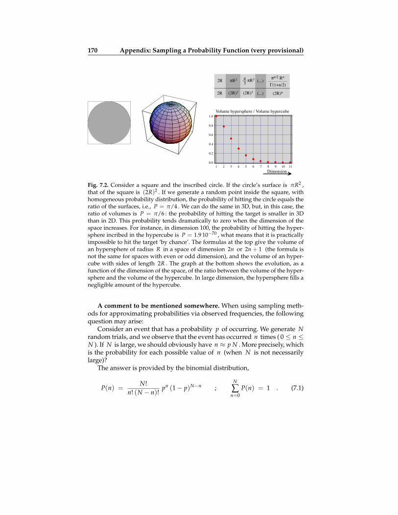
170 Appendix: Sampling a Probability Function (very provisional)
Dimension1 2 3 4 5 6 7 8 9 10 11
Volume hypersphere / Volume hypercube
0.6
0.4
0.2
0.0
0.8
1.0
2R 43
πR3πR2
2R (2R)2 (2R)n(2R)3
(...)
(...)
πn/2 Rn
Γ(1+n/2)
Fig. 7.2. Consider a square and the inscribed circle. If the circle’s surface is πR2 ,that of the square is (2R)2 . If we generate a random point inside the square, withhomogeneous probability distribution, the probability of hitting the circle equals theratio of the surfaces, i.e., P = π/4 . We can do the same in 3D, but, in this case, theratio of volumes is P = π/6 : the probability of hitting the target is smaller in 3Dthan in 2D. This probability tends dramatically to zero when the dimension of thespace increases. For instance, in dimension 100, the probability of hitting the hyper-sphere incribed in the hypercube is P = 1.9 10−70 , what means that it is practicallyimpossible to hit the target ‘by chance’. The formulas at the top give the volume ofan hypersphere of radius R in a space of dimension 2n or 2n + 1 (the formula isnot the same for spaces with even or odd dimension), and the volume of an hyper-cube with sides of length 2R . The graph at the bottom shows the evolution, as afunction of the dimension of the space, of the ratio between the volume of the hyper-sphere and the volume of the hypercube. In large dimension, the hypersphere fills anegligible amount of the hypercube.
A comment to be mentioned somewhere. When using sampling meth-ods for approximating probabilities via observed frequencies, the followingquestion may arise:
Consider an event that has a probability p of occurring. We generate Nrandom trials, and we observe that the event has occurred n times ( 0 ≤ n ≤N ). If N is large, we should obviously have n ≈ p N . More precisely, whichis the probability for each possible value of n (when N is not necessarilylarge)?
The answer is provided by the binomial distribution,
P(n) =N!
n! (N − n)!pn (1− p)N−n ;
N
∑n=0
P(n) = 1 . (7.1)

7.1 Sampling a Probability 171
7.1.4 Notion of Sample
Let M be a finite-dimensional metric manifold, with points denoted P0 , P , . . . .Let dv(P) represent the volume element of the manifold. If f (P) is a nor-malized volumetric probability over M , then, by definition, the probabilityof a domain A ⊂ M is
P(A) =∫
Adv(P) f (P) . (7.2)
Assume that some random process (mathematical or physical) generatesone random point P0 on M . The random point P0 is called a sample ofthe probability distribution f (P) if the probability that P0 belongs to anysubset A of M equals P(A) .
7.1.5 Inversion Method
Consider a (1D) volumetric probability f (x) depending on a scalar variablex , with length element ds(x) . This may occur when we have really onesingle random variable or, more often, when on a multidimensional man-ifold we consider a conditional distribution on a line (along which x is aparameter). The ‘inversion method’ consists in introducing the cumulativeprobability
y = F(x) =∫ x
xmin
ds(x′) f (x′) , (7.3)
that takes values in the interval [0, 1] , and the inverse function x = F−1(y) .It is easy to see that if one randomly generates values of y with constantprobability density in the interval [0, 1] , then the values x = F−1(y) arerandom samples ‘of’ the volumetric probability f (x) . Provided the functionF−1 is available, the method is simple and efficient.
Example 7.2 Let y1 , y2 . . . be samples of a random variable with constant vol-umetric probability in the interval [0, 1] , and let erf−1 be the inverse error func-tion2. The numbers erf−1(y1) , erf−1(y1) . . . are then normally distributed, withzero mean and unit variance (see figure 7.3).
7.1.6 Rejection Method
The ‘rejection method’ starts by generating samples x1 , x2 . . . of the homo-geneous volumetric probability, which usually is a simple problem. Then,
2 The error function erf(x) is the integral between −∞ and x of a normalizedGaussian with zero mean and unit variance (be careful, there are different defini-tions). One may find in the literature different series expressions for erf−1 .

172 Appendix: Sampling a Probability Function (very provisional)
Fig. 7.3. Use of the ‘inversion method’ to producesamples of a two-dimensional Gaussian volumetricprobability.
0
0
1
1
0
0
+3
+3
−3
−3
each sample is submitted to the possibility of a rejection: the probability thatthe sample xk is accepted being taken equal to
P =f (xk)fmax
, (7.4)
where fmax stands for the maximum of all the values f (x) , or any largernumber (the larger the number, the less efficient the method). It is then easyto prove that any accepted point is a sample of the volumetric probabilityf (x) .
This methods works reasonably well in one dimension or two dimen-sions, and could, in principle, be applicable in any number of dimensions.But, as already mentioned, large-dimensional spaces tend to be very empty,and the chances that this method accepts a point may be dramatically lowwhen working with multi-dimensional spaces.
7.1.7 Sequential Realization
In equation 6.70 (page 142), we have expressed a joint volumetric probabil-ity as the product of a conditional times a marginal. The conditional itselfmay sometimes be also further decomposed, and so on, until one has anexpression like
fn(x1, x2, . . . , xn) == f1(x1) f1|1(x2|x1) f1|2(x3|x1, x2) . . . f1|n−1(xn|x1, . . . , xn−1) ,
(7.5)
where each of the xi is, in general, multidimensional.All these marginal and conditional volumetric probabilities are con-
tained in the original n-dimensional joint volumetric probability fn(x1, x2, . . . , xn) ,and can, at least in principle, be evaluated from it using integrals. Assumethat they are all known, and let us see how an n-dimensional sample couldbe generated.
One starts generating a sample for the (perhaps multidimensional) vari-able x1 , using the marginal f1(x1) , this giving a value x0
1 . With this valueat hand, one generates a sample for the variable x2 , using the conditionalf1|1(x2|x0
1) , this giving a value x02 . Then, one generates a sample for the
variable x3 , using the conditional f1|2(x3|x01, x0
2) , this giving a value x03 .
And so on until one generates a sample for the variable xn , using the con-ditional f1|n−1(xn|x0
1, . . . , x0n−1) , this giving a value x0
n . In this manner a

7.2 Monte Carlo (Sampling) Methods 173
point x01, x0
2, . . . , x0n has been generated that is a sample of the original
fn(x1, x2, . . . , xn) .
7.2 Monte Carlo (Sampling) Methods
7.2.1 Random Walks and the Metropolis Rule
Blind random search in multidimensional spaces may be very inefficient,as already mentioned. This is why, when the probability distribution to besampled is relatively uncomplicated, one may use a ‘random walk’, a sortof Brownian motion where the probability of getting lost in the vast empti-ness of multidimensional spaces is kept low. When this works, this worksvery well, but this is not panacea: for really complicated probability distri-butions, with isolate regions of significant probability, this may not work atall: the discovery of these isolated regions is an intrinsically difficult prob-lem, where mathematics alone are not of much help. It is only the carefulconsideration of the physics involved in the problem, and of the particularproperties of the probability distribution that may suggest some strategy.This strategy shall be problem dependent.
In what follows, then, we concentrate in moderately complicated proba-bility distributions, where random walks are appropriate for sampling. Weanalyze here the random walks without memory: each step depends onlyon the last step. Such a walk without memory is technically called a MarkovChain Monte Carlo (MCMC) random walk.
7.2.2 Modification of Random Walks
Assume here that we can start with a random walk that samples some nor-malized volumetric probability f (P) , and have the goal of having a randomwalk that samples the volumetric probability
h(P) =1ν
f (P) g(P) , (7.6)
i.e., the conjunction of f with some other volumetric probability g . Here, νis the normalizing factor ν =
∫M dv(P) f (P) .
Call Pi the ‘current point’. With this current point as starting point, runone step of the random walk that unimpeded would sample the volumetricprobability f (P) , to generate a ‘test point’ Ptest . Compute the value
g(Ptest) . (7.7)
If this value is ‘high enough’, let the point Ptest ‘survive’. If g(Ptest) is not‘high enough’, discard this point and generate another one (making another

174 Appendix: Sampling a Probability Function (very provisional)
step of the random walk sampling the prior volumetric probability f (P)) ,using again Pi as starting point).
There are many criteria for deciding when a point should survive orshould be discarded, all of them resulting in a collection of ‘surviving points’that are samples of the target volumetric probability h(P) . For instance, ifwe know the maximum possible value of g(P) , say g(P)max , then define
Ptest =g(Ptest)g(P)max
, (7.8)
and give the point Ptest the probability Ptest of survival (note that 0 <Ptest < 1 ). It is intuitively obvious why the random walk modified usingsuch a criterion produces a random walk that actually samples the volumet-ric probability h(P) defined by equation 7.6.
Among the many criteria that can be used, the by far most efficient is theMetropolis criterion, the criterion behind the Metropolis Algorithm (Metropo-lis et al. 1953). In the following we shall describe this algorithm with somedetail.
7.2.3 The Metropolis Rule
Consider the following situation. Some random rules define a random walkthat samples the volumetric probability f (P) . At a given step, the randomwalker is at point Pi , and the application of the rules would lead to a tran-sition to point Pj . If that ‘proposed transition’ Pi → Pj is always accepted,the random walker will sample the volumetric probability f (P) . Instead ofalways accepting the proposed transition Pi → Pj , we reject it sometimesby using the following rule to decide if the random walker is allowed tomove to Pj of if it must stay at Pi :
– if g(Pj) ≥ g(Pi) , then accept the proposed transition to Pj ,– if g(Pj) < g(Pi) , then decide randomly to move to Pj , or to stay at Pi ,
with the following probability of accepting the move to Pj :
P =g(Pj)g(Pi)
. (7.9)
Then we have the following
Theorem 7.1 The random walker samples the conjunction h(P) of the volumetricprobabilities f (P) and g(P)
h(P) = k f (P) g(P) (7.10)
(see appendix ?? for a demonstration).
The algorithm above is reminiscent (see appendix ??) of the Metropolisalgorithm (Metropolis et al., 1953), originally designed to sample the Gibbs-Boltzmann distribution. Accordingly, we will refer to the above acceptancerule as the Metropolis rule.

7.2 Monte Carlo (Sampling) Methods 175
7.2.4 The Cascaded Metropolis Rule
As above, assume that some random rules define a random walk that sam-ples the volumetric probability f1(P) . At a given step, the random walkeris at point Pi ;
1 apply the rules, that unthwarted, would generate samples of f1(P) , topropose a new point Pj ,
2 if f2(Pj) ≥ f2(Pi) , go to point 3; if f2(Pj) < f2(Pi) , then decide ran-domly to go to point 3 or to go back to point 1, with the following prob-ability of going to point 3: P = f2(Pj)/ f2(Pi) ;
3 if f3(Pj) ≥ f3(Pi) , go to point 4; if f3(Pj) < f3(Pi) , then decide ran-domly to go to point 4 or to go back to point 1, with the following prob-ability of going to point 4: P = f3(Pj)/ f3(Pi) ;
. . . . . .n if fn(Pj) ≥ fn(Pi) , then accept the proposed transition to Pj ; if fn(Pj) <
fn(Pi) , then decide randomly to move to Pj , or to stay at Pi , with thefollowing probability of accepting the move to Pj : P = fn(Pj)/ fn(Pi) ;
Then we have the following
Theorem 7.2 The random walker samples the conjunction h(P) of the volumetricprobabilities f1(P), f2(P), . . . , fn(P) :
h(P) = k f1(P) f2(P) . . . fn(P) . (7.11)
(see appendix XXX for a demonstration).
7.2.5 Initiating a Random Walk
Consider the problem of obtaining samples of a volumetric probability h(P)defined as the conjunction of some volumetric probabilities f1(P), f2(P), f3(P) . . . ,
h(P) = k f1(P) f2(P) f3(P) . . . , (7.12)
and let us examine three common situations.We may start with a random walk that actually samples f1(P) . Then, a
direct application of the cascaded Metropolis rule allows to produce samplesof h(P) .
Sometimes, we do not have readily available a random walk that sam-ples f1(P) . In that case, we rewrite expression 7.12 as
h(P) = k f0(P) f1(P) f2(P) f3(P) . . . , (7.13)
where f0(P) is the homogeneous volumetric probability. Because we usevolumetric probabilities (and not probability densities), f0(P) is just a con-stant3. Then, the first cascade of the cascaded Metropolis algorithm providesthe random walk that samples f1(P) , and we can proceed ‘as usual’.
3 Whose value is the inverse of the total volume of the manifold.

176 Appendix: Sampling a Probability Function (very provisional)
In the worst circumstance, we only have a random walk that samplessome volumetric probability ψ(P) that is not of interest to us. Rewritingexpression 7.12 as
h(P) = k ψ(P)f0(P)ψ(P)
f1(P) f2(P) f3(P) . . . , (7.14)
immediately suggests to use the cascaded Metropolis algorithm to pass froma random walk that samples ψ(P) to a random walk that samples the ho-mogeneous volumetric probability f0(P) , then to a random walk that sam-ples f1(P) , and so on.
7.2.6 Choosing Random Directions and Step Lengths
A random walk is an iterative process where, when we stay at some ‘currentpoint’, we may jump to a neighboring point. We must decide two things, thedirection of the jump and its step length. Let us examine the two problemsin turn.
7.2.6.0.1 Choosing Random Directions
When the number of dimensions is small, a ‘direction’ in a space is some-thing simple. This is not so when we work in large-dimensional spaces.Consider, for instance, the problem of choosing a direction in a space offunctions. Of course, a space where each point is a function is infinite-dimensional, and we work here with finite-dimensional spaces, but we mayjust assume that we have discretized the functions using a large number ofpoints, say 10 000 or 10 000 000 points.
If we are ‘at the origin’ of the space, i.e., at point 0, 0, . . . represent-ing a function that is everywhere zero, we may decide to choose a directionpointing towards smooth functions, or fractal functions, gaussian-like func-tions, functions having zero mean value, L1 functions, L2 functions, func-tions having a small number of large jumps, etc. This freedom of choice,typical of large-dimensional problems, has to be carefully analyzed, and itis indispensable to take advantage of it whe designing random walks.
Assume that we are able to design a random walk that samples the vol-umetric probability f (P) , and we wish to modify it considering the valuesg(P) , using the Metropolis rule (or any equivalent rule), in order to obtaina random walk that samples
h(P) = k f (P) g(P) . (7.15)
We can design many initial random walks that sample f (P) . UsingMetropolis modification of a random walk, we will always obtain a randomwalk that samples h(P) . A well designed initial random walk will ‘present’to the Metropolis criterion test points Ptest that have a large probability of

7.3 Random Points on the Surface of the Sphere 177
being accepted (i.e., that have a large value of g(Ptest) ). A poorly designedinitial random walk will test points with a low probability of being accepted.Then, the algorithm is very slow in producing accepted points. Althoughhigh acceptance probability can always be obtained with very small steplengths (if the volumetric probability to be sampled is smooth), we needto discover directions that give high acceptance ratios even for large steplengths.
7.2.6.0.2 Choosing Step Lengths
Numerical algorithms are usually forced to compromise between some con-flicting wishes. For instance, a gradient-based minimization algorithm hasto select a finite step length along the direction of steepest descent. Thelarger the step length, the smaller may be the number of iterations requiredto reach the minimum, but if the step length is chosen too large, we may loseefficiency; we can even increase the value of the target function, instead ofdiminishing it.
The random walks contemplated here face exactly the same situation.The direction of the move is not deterministically calculated, but is chosenrandomly, with the common-sense constraint discussed in the previous sec-tion. But once a direction has been decided, the size of the jump along thisdirection, that has to be submitted to the Metropolis criterion, has to be ‘aslarge as possible’, but not too large. Again, the ‘Metropolis theorem’ guar-antees that the final random walk will sample the target probability distri-bution, but the better we are in choosing the step length, the more efficientthe algorithm will be.
In practice, a neighborhood size giving an acceptance rate of 30%− 60%(for the final, posterior sampler) can be recommended.
7.3 Random Points on the Surface of the Sphere
Fig. 7.4. 1000 random points on the surface of the sphere.
Note: Figure 7.4 has been generated using the following Mathematicacode:
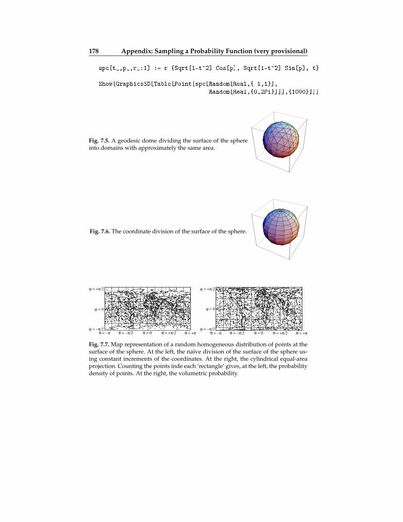
178 Appendix: Sampling a Probability Function (very provisional)
spc[t_,p_,r_:1] := r Sqrt[1-t^2] Cos[p], Sqrt[1-t^2] Sin[p], t
Show[Graphics3D[Table[Point[spc[Random[Real,-1,1],
Random[Real,0,2Pi]]],1000]]]
Fig. 7.5. A geodesic dome dividing the surface of the sphereinto domains with approximately the same area.
Fig. 7.6. The coordinate division of the surface of the sphere.
θ = 0
ϕ = 0
θ = −π/2ϕ = −π/2
θ = −π θ = +π
ϕ = +π/2
θ = +π/2 θ = 0
ϕ = 0
θ = −π/2ϕ = −π/2
θ = −π θ = +π
ϕ = +π/2
θ = +π/2
Fig. 7.7. Map representation of a random homogeneous distribution of points at thesurface of the sphere. At the left, the naïve division of the surface of the sphere us-ing constant increments of the coordinates. At the right, the cylindrical equal-areaprojection. Counting the points inde each ‘rectangle’ gives, at the left, the probabilitydensity of points. At the right, the volumetric probability.

8 Appendix: Demonstrations
8.1 Compatibility Property
8.1.1 Proof of the Compatibility Property (Sets)
Let us here demonstrate the property that, if ϕ represents a mapping froma set A0 into a set B0 , then, for any A ⊆ A0 and for any B ⊆ B0 ,
ϕ[ A∩ ϕ-1[ B ] ] = ϕ[A]∩B . (8.1)
The demonstration is made as follows. We first consider an element that be-longs to the set ϕ[ A∩ ϕ-1[ B ] ] , and demonstrate that it necessarily belongsto the set ϕ[A]∩B . We then consider an element of the set ϕ[A]∩B , anddemonstrate that it necessarily belongs to the set ϕ[ A∩ ϕ-1[ B ] ] . This willprove that two sets are identical.
So consider an element y ∈ ϕ[ A∩ ϕ-1[ B ] ] . This implies that there isan x with ϕ(x) = y , such that x ∈ A and x ∈ ϕ-1[B] . But x ∈ A andx ∈ ϕ-1[B] implies ϕ(x) ∈ ϕ[A] and1 ϕ(x) ∈ B , which, in turn, implies y ∈ϕ[A] and y ∈ B , i.e., y ∈ ϕ[A]∩B , and the first part of the demonstrationis done. Consider now an element y ∈ ϕ[A]∩B . This implies that thereis an x such that x ∈ A and ϕ(x) ∈ B , i.e., x ∈ A and x ∈ ϕ-1[B] ,so x ∈ A∩ ϕ-1[B] . Then, necessarily, y = ϕ(x) ∈ ϕ[ A∩ ϕ-1[ B ] ] , and thesecond part of the demonstration is also done.
8.1.2 Proof of the Compatibility Property (Probabilities)
8.1.2.1 Discrete Sets
Let A0 and B0 be two discrete sets. We wish to satisfy the condition that forany mapping ϕ from A0 into B0 , for any two probabilities P (over A0 )and Q (over B0 ), and for any element b ∈ B0 ,
( ϕ[ P∩ ϕ-1[Q] ] )[ b ] = ( ϕ[P] ∩Q )[ b ] . (8.2)
Using equation 2.49 (image of a probability), we can write the left-hand sideof this expression as
1 One always has ϕ[ϕ-1[B]] ⊆ B (equation 1.14 page 7).

180 Appendix: Demonstrations
( ϕ[ P∩ ϕ-1[Q] ] )[ b ] = ∑a∈ϕ-1[b]
( P∩ ϕ-1[Q] )[a] , (8.3)
and, using equation 2.38 (intersection of probabilities),
( ϕ[ P∩ ϕ-1[Q] ] )[ b ] =1ν ∑
a∈ϕ-1[b]P[a] ( ϕ-1[Q] )[a] , (8.4)
where ν is a normalization constant. Let us now take the right-hand side.Using equation 2.38 (intersection of probabilities) gives
( ϕ[P] ∩Q )[ b ] =1ν′
( ϕ[P])[ b ] Q[ b ] , (8.5)
where ν′ is a normalization constant. Using equation 2.49 (image of a prob-ability) gives
( ϕ[P] ∩Q )[ b ] = =1ν′
(∑
a∈ϕ-1[b]P[a]
)Q[ b ] , (8.6)
or, equivalently,
( ϕ[P] ∩Q )[ b ] =1ν′ ∑
a∈ϕ-1[b]P[a] Q[ ϕ(a) ] . (8.7)
The two expressions at the right-hand side of equations 8.4 and equation 8.7can be made identical (for any probability P and any element b ) if, andonly if, one defines the reciprocal image of a probability via
( ϕ-1[Q] )[a] =1
ν′′Q[ ϕ(a) ] , (8.8)
where ν′′ is a normalization constant (this is exactly the definition used inequation 2.63). With this definition, expression 8.2 holds (for any mappingϕ , for any two probabilities P and Q , and for any element b ).
8.1.2.2 Manifolds
Consider a mapping ϕ from a p-dimensional manifold Mq into a q-dimensionalmanifold Mq . Both manifolds are assumed to have a volume measure func-tion defined.
Basic equations are 2.50
g = ϕ[ f ] ⇔ g(y) = ∑x∈ϕ-1[y]
f (x)|det Φ(x)| , (8.9)
and 2.52

8.1 Compatibility Property 181
g = ϕ[ f ] ⇔
g(y) =∫
ε12...(p−q) dz1 dz2 . . . dzp−q f (x(y, z)) |det Ψ(y, z)| ,(8.10)
Let us start from the expression 2.59 giving the image of a volumetricprobability function,
g(Q) = ∑P∈ϕ-1[Q]
f (P) α(P) , (8.11)
where α(P) is a function whose expression shall not be needed here. Wemust also use the expression for the intersections of the probability densityfunctions (equation 2.39):
( f ∩ f ′)(P) =1ν
f (P) f ′(P) , (g∩ g′)(Q) =1ν
g(Q) g′(Q) . (8.12)
We wish to satisfy the condition that for any mapping ϕ from Mq intoMq , for any two volumetric probabilities f (over Mq ) and g (over Mq ),and at any point Q ∈ Mq ,
( ϕ[ f ∩ ϕ-1[g] ] )(Q) = ( ϕ[ f ] ∩ g )(Q) . (8.13)
Using equation 8.11 (image of a probability), we can write the left-handside of this expression as
( ϕ[ f ∩ ϕ-1[g] ] )(Q) = ∑P∈ϕ-1[Q]
( f ∩ ϕ-1[g])(P) α(P) , (8.14)
and, using the first of equations 8.12 (intersection of probabilities),
( ϕ[ f ∩ ϕ-1[g] ] )(Q) =1ν ∑
P∈ϕ-1[Q]f (P) (ϕ-1[g])(P) α(P) , (8.15)
where ν is a normalization constant.Let us now take the right-hand side. Using the second of equations 8.12
(intersection of probabilities) gives
( ϕ[ f ] ∩ g )(Q) =1ν′
(ϕ[ f ])(Q) g(Q) , (8.16)
where ν′ is a normalization constant. Using equation 8.11 (image of a prob-ability) gives
( ϕ[ f ] ∩ g )(Q) =1ν′
(∑
P∈ϕ-1[Q]f (P) α(P)
)g(Q) , (8.17)
or, equivalently,

182 Appendix: Demonstrations
( ϕ[ f ] ∩ g )(Q) =1ν′ ∑
P∈ϕ-1[Q]f (P) g(ϕ(P)) α(P) , (8.18)
The two expressions at the right-hand side of equations 8.15 and 8.18 canbe made identical (for any probability density f and any point y ) only if —whatever the function α(P) may be— the reciprocal image of a volumetricprobability is given by
(ϕ-1[g])(x) =1
ν′′g(ϕ(P)) , (8.19)
where ν′′ is a normalization constant. This demonstrates both, the there isa unique solution for the reciprocal image of a volumetric probability thatsatisfies the compatibility condition (expression 8.13), and that its expressionis that given in equation 2.64 of the main text.
Note that in the demonstration of the property ϕ[ f ∩ ϕ-1[g] ] = ϕ[ f ]∩ gwe have not cared about the relative values of p and q , while we may bedoing the intersection of volumetric probabilities of different dimension. Infact, because there are the constants ν, ν′, . . . in the demonstration, there is akind of “automatic renormalization”, so we don’t need to take into accountthe relative values of p and q . For an illustration of this point, see the ex-ample in section 2.5.2, where Gaussian distributions (over linear spaces) areconsidered.

8.2 Image of a Probability Density 183
8.2 Image of a Probability Density
8.2.1 New Example
Consider a two-dimensional manifold M endowed with some coordinatesx1, x2 = u, v , both taking values in the domain (−∞, +∞) , and a map-ping ϕr from M into the real line < :
u, v 7→ r = ϕr(u, v) . (8.20)
Let f (u, v) be a probability density over M . Which is the image, say g(r) ,of f (u, v) via ϕr ? The answer is obtained as follows. We momentarily in-troduce the manifold <2 = < × < and complete the mapping ϕr to havea bijective mapping (I think that I can always choose ϕs to have a bijectivemapping) from M into <2 :
r = ϕr(u, v)s = ϕs(u, v) .
(8.21)
As the mapping is bijective, we can obtain u, v as a function of r, s :
u = u(r, s)v = v(r, s) .
(8.22)
The image of f (u, v) in <2 is easy to obtain, as a bijective mapping can beseen as a change of variables:
g2(r, s) = f ( u(r, s) , v(r, s)) |det
(∂u/∂r ∂u/∂s∂v/∂r ∂v/∂s
)| (8.23)
Then, the solution to our problem is obtained by marginalization:
g(r) =∫ +∞
−∞ds g2(r, s) . (8.24)
(Note: I have to justify here the fact that the result is independent of thechoice of function ϕs(u, v) . It is chosen in a way that (i) one has a bijection,and (ii) the computations are simple.)
As a numerical example, consider that M is a linear manifold, f (u, v) isa Gaussian, and the mapping ϕr is r = ϕr(u, v) = u2 + v . As the sign of uis lost in this mapping, a good choice for the mapping ϕs(u, s) is
r = ϕr(u, v) = u2 + vs = ϕs(u, v) = u ,
(8.25)
with the reciprocal equations

184 Appendix: Demonstrations
u = s
v = r− s2 .(8.26)
The function ϕs has the suppelmentary advantage of giving the value 1 tothe Jacobian in equation 8.23.
Figure 8.1 displays the original Gaussian f (u, v) , with the functionsr(u, v) and s(u, v) suggested. Figure 8.2 displays the function g2(r, s) de-fined by the considered mapping. Finally, figure 8.3 displays the probabilitydensity g(r) that is the answer to the original question: what is the imageof f (u, v) via the mapping r = u2 + v ?
Fig. 8.1. The original Gaussian f (u, v) , with thefunctions r(u, v) and s(u, v) suggested.
r = 2
r = 0r = -2
u = 2u = 0
u = -2
v = 2
v = 0
v = -2
s = -2
s = 0
s = 2
Fig. 8.2. The function g2(r, s) defined by theconsidered mapping.
r = 4
r = 8
r = 0
s = 2
u = 0
u = -2
u = 2
s = 0
s = -2
v = 4
v = -4
The final question is: how all this modifies the “demonstration” I havefor the compatibility property?

8.2 Image of a Probability Density 185
Fig. 8.3. The probability density g(r) that is theanswer to the original question: what is the im-age of f (u, v) via the mapping r = u2 + v ?
0
0.2
0.4
r = 0
r = 5
r = 10

186 Appendix: Demonstrations
8.2.2 Old Text
We shall demonstrate here equation 2.52 given in example 2.18 (page 28).Consider a mapping ϕ from a p-dimensional manifold Mp into a q-dimen-sional manifold Mq . Take some coordinates x ≡ xi, . . . , xp over Mq andsome coordinates y ≡ yi, . . . , yq over Mq , and introduce the Jacobianmatrix Φi
α = ∂yi/∂xα . Let P be a probability function over Mq , repre-sented by the probability density function f (x) , and let Q = ϕ[P] be theimage of P via the mapping ϕ . If p ≥ q , the probability function Q = ϕ[P]can be represented by a probability density function, say (ϕ[ f ])(y) . Wehave to demonstrate here that at any point y ∈ Mq where det(Φ Φt) 6= 0one has
g = ϕ[ f ] ⇔ g(y) = ∑x∈ϕ-1[y]
f (x)√det(Φ(x) Φ(x)t)
. (8.27)
So, to every probability function P defined over (a σ-field of subsetsof) Mp , the mapping ϕ associates its image Q = ϕ[P] , the probabilityfunction over Mq , defined in section 2.3 through the condition
Q = ϕ[P] ⇔ Q[ B ] = P[ ϕ-1[ B ] ] , (8.28)
the expression at the right having to hold for any set B ⊆ Mq .We are not assuming here that the manifolds into consideration have
a notion of volume defined, so we must use probability densities (i.e., weshould not try to use volumetric probabilities). Assume, then, that a co-ordinate system x = xα = x1, . . . , xp has been introduced over Mp
and a coordinate system y = yi = y1, . . . , yq = y1, . . . , yp hasbeen introduced over Mq . These coordinate systems may, of course, not beglobal, but this is a traditional complication that we do not need to addresshere. In terms of the coordinates of a point, the mapping ϕ can be writtenx 7→ y = ϕ(x) . Introducing the two probability densities that represent Pand Q as
P[A] =∫
Aε12...p dx1 dx2 . . . dxp f (x1, . . . , xp)
Q[B] =∫
Bε12...p dy1 dy2 . . . dyq g(y1, . . . , yq) ,
(8.29)
our problem here is to express the function g(y) in terms of the functionf (x) .
There are two interesting situations, p = q , and p > q . When p <q , the density is singular, and the computations are better done withoutintroducing g(y) (see the example in section 2.5.3).

8.2 Image of a Probability Density 187
Case p = q .
In this case, the two manifolds have the same dimension (and the mappingx 7→ y = ϕ(x) is assumed to be “non pathological”), the coordinate systemin the neighborhood of any point x ∈ Mp defines (via the mapping ϕ ) acoordinate system in the neighborhood of the point y = ϕ(x) ∈ Mq . Then,in the neighborhood of the point y ∈ Mq we can compare two coordinatesystems, the original coordinates yi and the “image” on Mq of the co-ordinates xα of Mp . With this in mind, one cas see that the problem ofevaluating the image g = ϕ[ f ] of a probability density f defined over Mpis formally identical to the problem of analyzing the change of a probabilitydensity under a change of variables on a manifold. (Note: I must [strongly]say somewhere that many problems of “change of variables” are, in fact, aproblem of “image of a probability”. When we use a mathematical definition,like x = log X , we do face a change of variables, but when we use a physi-cal relation, we do not.) For an actual change of variables, that is a bijection,the result is (equation 9.237)
f′(x′) =
f (x)|X′(x) | ; ( x′ = x′(x) ) , (8.30)
where
X′i′i(x) =
∂xi′
∂xi (x) ; X′(x) = det X′(x) . (8.31)
Equation 8.30 suggests that the solution to our problem may be
g = ϕ[ f ] ⇔ g(y) = ∑x∈ϕ-1[y]
f (x)|Y(x) | , (8.32)
the expression at the right holding for any point y ∈ Mq . Here, the sum isover all the points x on Mp that map into the same point y on Mq (thissum would not be present if we had a bijection), and
Yiα(x) =
∂ϕi
∂xα(x) ; Y(x) = det Y(x) . (8.33)
To verify that the defining condition 8.28 is satisfied, we can write thefollowing sequence of identities:

188 Appendix: Demonstrations
Q[ B ] =∫
Bdy1 ∧ · · · ∧ dyp g(y)
=∫
Bdy1 ∧ · · · ∧ dyp ∑
x∈ϕ-1[y]
f (x)|Y(x) |
= ∑α
∫ϕ-1[B]∩Mα
p
dx1 ∧ · · · ∧ dxp f (x)
=∫∪α(ϕ-1[B]∩Mα
p)dx1 ∧ · · · ∧ dxp f (x)
=∫
ϕ-1[B]dx1 ∧ · · · ∧ dxp f (x)
= P[ ϕ-1[ B ] ] .
(8.34)
Here, the sets Mαp represent the partition of Mp the set ϕ-1[B] that par-
titions the mapping ϕ into a sequence of injections (and, in this case, asp = q , of bijections) (see figure 8.4).
Fig. 8.4. When considering a mapping betweentwo manifolds with same dimension, one canpartition the reciprocal image A = ϕ-1[ B ] ofa set B into sets A1, A2, . . . such the mappingbetween each of the Aα and B is a bijection.
B
A1A2 A3 A4 A5
Case p > q :
In this case, the dimension of the departure manifold is larger than the di-mension of the arrival manifold, so we are in the situation suggested in fig-ure 8.5. The image of a probability density f (x1, . . . , xp) is a bona fide prob-ability density g(y1, . . . , yq) . It can be evaluated by, first, using the trick ofintroducing some “slack variables”, and, second, marginalizing them.
Fig. 8.5. When the dimension ofthe departure manifold is greaterthan the dimension of the arrivalmanifold. . .
y1
y2 g(y1,y2) = ?f(x1,x2,x3)
x1
x2
x3
y = ϕ(x) Bϕ-1[B]
Q[B] = P[ ϕ-1[B] ]
_ _
8.2 Image of a Probability Density 189
Let us see this with some detail. The simplest way to address this prob-lem consists in introducing a “slack manifold” Mp−q , whose dimension isp− q , and whose coordinates may be denoted yI = yq+1, . . . , yp . We cancomplete the q functions yi = ϕi(x1, . . . , xp) by some other (well chosen,but arbitrary) p− q functions yI = ϕI(x1, . . . , xp) , in order to have p func-tions depending on p variables:
initial functions :
y1 = ϕ1(x1, . . . , xp)· · · = · · ·yq = ϕq(x1, . . . , xp)
arbitrary functions :
yq+1 = ϕq+1(x1, . . . , xp)· · · = · · ·yp = ϕp(x1, . . . , xp) .
(8.35)
So we have now a mapping from the p-dimensional manifold Mp into thep-dimensional manifold Mq ×Mp−q , and this is the case examined in theprevious section, so the equations found there apply here. Therefore, for the(p-dimensional) image of the probability density f one has (equation 8.32)
gp(y) = ∑x∈ϕ-1[y]
f (x)|Y(x) | . (8.36)
Then we obtain the desired (q-dimensional) probability density function bymarginalization:
g(y1, . . . , yq) =∫
dyq+1 ∧ · · · ∧ dyp gp(y1, . . . , yq, yq+1, . . . , yp) . (8.37)
Of course, we need to verify that this marginal probability density does notdepend on the choice of the slack variables yq+1, . . . , yp . But this is obvi-ous, as changing from these variables into some other variables would justamount to an ordinary change of integration variables in equation 8.37.
It remains to prove here that we arrive at equation 8.27:
g = ϕ[ f ] ⇔ g(y) = ∑x∈ϕ-1[y]
f (x)√det(Φ(x) Φ(x)t)
. (8.38)
Example 8.1 Two quantities X, Y can take any real positive value, and, associ-ated to them is the (two-dimensional lognormal) probability density function
f (X, Y) =1
2 π σ21
X Yexp
(− 1
2log(X/X0)2 + log(Y/Y0)2
σ2
). (8.39)
Which is the probability density for the real positive quantity U = X/Y ? To usethe first method described above, we can introduce another real positive quantity,V = X Y . Using the Jacobian rule for the change of variables, one obtains

190 Appendix: Demonstrations
g2(U, V) =1
2 π Σ21
U Vexp
(− 1
2log(U/U0)2 + log(V/V0)2
Σ2
), (8.40)
with
U0 = X0/Y0 ; V0 = X0 Y0 ; Σ =√
2 σ , (8.41)
and computing the marginal g(U) =∫ ∞
0 dV g2(U, V) gives the result we weresearching:
g(U) =1√
2 π Σ1U
exp(− 1
2log(U/U0)2
Σ2
). (8.42)
If instead of choosing V = X Y we would have chosen V = X , we would havearrived to the probability density
g2(U, V) =1
2 π σ21
U Vexp
(− 1
2
(log(U/U0)log(V/V0)
)tC-1
(log(U/U0)log(V/V0)
) ),
(8.43)with
U0 = X0/Y0 ; V0 = X0 ; C = σ2(
2 11 1
), (8.44)
and, when computing the marginal g(U) , to the same result as above (as weshould). Finally, if we choose the alternative method suggested above, of the twovariables in f (X, Y) , we keep, for instance Y , and change X by U = X/Y . Thisleads to
g2(U, Y) =1
2 π σ21
U Yexp
(− 1
2
(log(U/U0)log(Y/Y0)
)tC-1
(log(U/U0)log(Y/Y0)
) ),
(8.45)with
U0 = X0/Y0 ; C = σ2(
2 −1−1 1
), (8.46)
and, when computing the marginal g(U) , again to the same result as above. Wecould have kept X , and change Y by U = X/Y .

9 Appendix: Complements (very provisional)
9.1 Toy Version of the Popper-Bayes Problem
In this book, most of the applications of probability theory concern a Bayesianinterpretation, where probabilities are used to represent “states of informa-tion”, or “degrees of belief”. This, of course is to be opposed to a “frequen-tist” use of probability theory, where probabilities are interpreted as the limitof “histograms”.
For theoretical developments, there is a clear advantage of the frequen-tist interpretation: most of the theorems can directly be checked by a directevaluation, and by taking the corresponding limit. This is why, dear Bar-tolomé, to state the problems you asked me to state, I have chosen to switchto frequentist problems. (By the way, it would be interesting to see if there isa kind of “correspondence principle”).
9.1.1 The Making of a Histogram (I)
Consider, then, a discrete and finite set, say A0 , with elements a1, a2, . . . , aN ,and some random algorithm that produces, on demand, sample elementsof A0 . For instance, if the algorithm is run n times, we may successivelyobtain a7, a1, a7, a7, a3 . . . . Alternatively, we may have n copies of the samealgorithm (with different “random seeds”) and run each algorithm once.When two two situations are “undistinguishable”, we say that the sampleelements are “independent”.
We can use the random algorithm to generate n sample elements, anddenote ki the number of time the element ai has materialized. The “exper-imental frequency” of ai is defined as f (ai; n) = ki/n . If when n → ∞ ,the experimental frequencies f (ai; n) converge to some definite values, sayp(ai) , then we say that the probability of element ai is p(ai) , and we write
p(ai) = limn→∞
f (ai; n) = limn→∞
kin
. (9.1)
Let A be a subset of A0 . The probability of the set A , denoted P[ A ] , isdefined, for obvious reasons, as

192 Appendix: Complements (very provisional)
P[ A ] = ∑a∈A
p(a) , (9.2)
where a denotes a generic element of A0 . One has P[ ∅ ] = 0 and P[ A0 ] =1 . The function P that to any set A ⊆ A0 associates the value P[ A ] iscalled a probability function (or, for short, a probability), while the numberP[ A ] is the probability value of the set A . For any a ∈ A0 , p(a) is the ele-mentary probability value of the element a .
9.1.2 The Making of a Histogram (II)
Assume that some random process generates consecutive points on a mani-fold (potentially an infinite number of them). To make a histogram, there aretwo ways. In the first way, one selects some coordinate system xα on themanifold, divides the manifold into small cells, by considering coordinateincrements ∆xα and counts the proportion of points that materialize intoeach cell. It is assumed that, when the number of points tends to infinity,these proportions converge to given numbers. The probability density rep-resenting the random process —in the given coordinates— is, by definition,the function f (x1, x2, . . . ) obtained as the limit of this histogram. Then, theprobability that “the next point” will materialize inside some domain A ofthe manifold is
P[A] =∫
Adω f (x1, x2, . . . ) , (9.3)
where the “capacity element” dω can be written, using two different nota-tions, as
dω = εα1α2 ...dxα1 dxα2 . . . = dx1 ∧ dx2 ∧ . . . . (9.4)
As an example, if the manifold is the surface of the sphere, and if we usespherical coordinates,
dω = dθ ∧ dϕ . (9.5)
The values of the function f are not invariant quantities. Under a change ofvariables, these values transform “as a density”, i.e., they are multiplied, ateach point, by the absolute value of the Jacobian of the transformation.
The second way exists when one has introduced a notion of volume overthe manifold. This practically corresponds to introducing a “volume den-sity” ω(x1, x2, . . . ) , and writing the “volume element” as
dω = ω dω . (9.6)
For instance, on the surface of the sphere, there is a notion of volume (in fact,of surface), and one writes
dω = ω dω = (r2 sin θ) (dθ ∧ dϕ) . (9.7)
Then, there is a second way for making a histogram, where, instead of di-viding the manifold into cells having the same “capacity” ∆ω , one divides

9.1 Toy Version of the Popper-Bayes Problem 193
the manifold into cells having the same volume ∆ω . For instance, on thesphere, this corresponds to introducing a geodesic triangulation of the sur-face of the sphere, all the triangles having the same surface. In the limitwhere the number of points tends to infinity, and the volume of the cellstends to zero, the histogram converges to another function, the volumetricprobability f (x1, x2, . . . ) . Then, the probability that “the next point” willmaterialize inside some domain A of the manifold is
P[A] =∫
Adω f (x1, x2, . . . ) . (9.8)
The values of the function f are invariant (i.e., independent of any choice ofcoordinates over the manifold). The relation between a probability densityand a volumetric probability is
f (x1, x2, . . . ) = ω(x2, x2, . . . ) f (x1, x2, . . . ) . (9.9)
For instance, on the surface of the sphere, with spherical coordinates,
f (θ, ϕ) = r2 sin θ f (θ, ϕ) . (9.10)
9.1.3 First Problem: Image of a Probability
Consider a mapping ϕ from a p-dimensional manifold Mp into a q-dimen-sional manifold Mq . The mapping is not assumed surjective (there may bepoints on Mq that can not be reached as images of points on Mp ) or to beinjective (there may be points on Mq that can be reached from more thanone point on Mp ).
When endowing Mp and Mq with respective coordinate systems, sayx ≡ xα = x1, . . . , xp and y ≡ yi = y1, . . . , yq , the mapping can bewritten x 7→ y = ϕ(x) .
A random process generates points on the first manifold, according tothe probability density f (x) . Each of these points is mapped into a pointon the second manifold. We thus also have random points on the secondmanifold. Question #1: which is the probability density g(y) that these randompoints define? (I state this problems in terms of probability densities because Ido not assume that volume elements have necessarily been introduced overthe manifolds).
As I have discussed elsewhere in this text (note: say where), there arethree different situation, p = q , p > q , and p < q . The case p > q is treatedby adding some “slack variables”, so, in fact, we are brought back to the casep = q . The case p < q is a little bit pathological (the probability densitytakes nonzero values on a submanifold of Mq ), and will not be examinedhere. So, let us assume p = q .

194 Appendix: Complements (very provisional)
Consider a tesselation of Mq in cells of constant capacity, ∆v = ∆y1 ∧· · · ∧ ∆yq . It is easy to see1 that to these cells corresponds, in Mp a tessela-tion in cells of variable capacity, given by
∆ω(x) =∆v
|Φ(x)| (9.11)
where
Φiα =
∂ϕi
∂xα; Φ = det Φ . (9.12)
The probability that a point materializes inside the capacity element ∆ω(x)at point x is ∆P(x) = f (x) ∆ω(x) . Now, which is the probability ∆Q thatan image point y = ϕ(x) materializes inside a capacity element ∆v at pointy ? As there may be more that one x such that ϕ(x) = y , this probability is∆Q(y) = ∑x∈ϕ-1[y] ∆P(x) , so we can write
∆Q(y) = ∑x∈ϕ-1[y]
∆P(x) = ∑x∈ϕ-1[y]
f (x) ∆ω(x)
= ∑x∈ϕ-1[y]
f (x)∆v
|Φ(x)| =(
∑x∈ϕ-1[y]
f (x)|Φ(x)|
)∆v .
(9.13)
Introducing, then, the probability density g(y) via
∆Q(y) = g(y) ∆v , (9.14)
immediately gives g(y) = ∑x∈ϕ-1[y] f (x) / |Φ(x)| . We can call this proba-
bility density g(y) the image of f (x) , and use the notation g = ϕ[ f ] . Then,we can write
g = ϕ[ f ] ⇔ g(y) = ∑x∈ϕ-1[y]
f (x)|Φ(x)| , (9.15)
the equality at the right-hand side holding for any y ∈ Mq .The probability function so defined over Mq does not depend, of course,
on the particular coordinates being used over Mp or over Mq . To see thisdirectly from equation 9.15, it is clear that if changing, in Mp , from the co-ordinates x to some other coordinates x′ = x′(x) , a Jacobian will appearthat will transform f (x) , into f ′(x′) , but this Jacobian will be absorbed bymatrix of partial derivatives, that will become the matrix of partial deriva-tives with respect to the new variables, so the form of the equation will be
1 This is just the multidimensional version of the fact that, from y = ϕ(x) , it followsdy = (dϕ/dx) dx .
9.1 Toy Version of the Popper-Bayes Problem 195
left invariant. That the probability function so defined over Mq is also inde-pendent from the coordinates y being used over Mq results directly fromthe fact that we recognize that g(y) is a density (so we know that whenchanging the coordinates over Mq the values g(y) have to be multipliedby the Jacobian of the transformation, this leaving the finite probabilitiesinvariant).
Associated to the two probability density functions f (x) and g(y) thereare two probability functions P and Q . They satisfy the simple property
Q = ϕ[P] ⇔ Q[ B ] = P[ ϕ-1[ B ] ] , (9.16)
the equality at the right holding for any set B ⊆ Mq . The demonstration isquite easy (for the time being, this is just a reproduction of equations 8.34):
Q[ B ] =∫
Bdy1 ∧ · · · ∧ dyp g(y)
=∫
Bdy1 ∧ · · · ∧ dyp ∑
x∈ϕ-1[y]
f (x)|Y(x) |
= ∑α
∫ϕ-1[B]∩Mα
p
dx1 ∧ · · · ∧ dxp f (x)
=∫∪α(ϕ-1[B]∩Mα
p)dx1 ∧ · · · ∧ dxp f (x)
=∫
ϕ-1[B]dx1 ∧ · · · ∧ dxp f (x)
= P[ ϕ-1[ B ] ] .
(9.17)
For completeness, let me mention that if there were volume elementsdefined, that in terms of the selected coordinates were written
dω = ω dω = ω dx1 ∧ · · · ∧ dxp
dv = v dv = v dy1 ∧ · · · ∧ dyq ,(9.18)
then we would be able to express equation 9.15 in terms of volumetric prob-abilities, say f (x1, . . . , xp) and g(y1, . . . , yq) , as follows:
g = ϕ[ f ] ⇔ g(y) =1
v(y) ∑x∈ϕ-1[y]
f (x) ω(x)|Φ(x)| . (9.19)
9.1.4 Second Problem: Intersection of Two Probabilities
Consider a manifold M with a notion of volume defined, and such thatthe total volume of the manifold is finite. Assume that two distinct random

196 Appendix: Complements (very provisional)
processes generate simultaneous random points on a manifold, accordingto the volumetric probabilities f1(P) and f2(P) . We have, in fact, randompairs of points. Dividing the manifold into cells of equal volume, say ∆ω ,one can build a histogram as follows: if the two points are on the same cell,the count of the cell is increased; if the two points belong to different cells,the points are ignored. In the limit of a large number of (pairs of) points, thisproduces a volumetric probability f (P) . Question #2: how is f (P) related tof1(P) and to f2(P) ?
The probability that the first point materializes inside the domain aroundsome point P is ∆P1(P) = f1(P) ∆ω , while the probability that secondpoint materializes inside the same domain is ∆P2(P) = f2(P) ∆ω . As thetwo event are independent, the total probability, say ∆P(P) , equals theproduct of the two probabilities,
∆P(P) = ∆P1(P) ∆P2(P) = f1(P) f2(P) (∆ω)2 . (9.20)
This is the probability that when two points are drawn, they materialize inthe volume around point P . A different question is: if we know that twopoints have materialized in the same volume around some point, which isthe probability that point is point P ? This question has the same answer asthe previous question, excepted that we must now normalize to one, so weobtain ∆P(P) = f1(P) f2(P) / ∑ f1(P′) f2(P′) , where the sum is over all thecells. Introducing the resulting volumetric probability f (P) via ∆P(P) =f (P) ∆ω gives f (P) ∆ω = f1(P) f2(P) / ∑ f1(P′) f2(P′) , i.e.,
f (P) =f1(P) f2(P)
∑ ∆ω f1(P′) f2(P′), (9.21)
and taking the limit ∆ω → 0 gives the result we were looking for:
f = f1 ∩ f2 ⇔ f (P) =f1(P) f2(P)∫
M dω f1(P′) f2(P′), (9.22)
where the equality at the right-hand side hold for any point P ∈ M .Note: it is essential here that the cells into which the manifold is defined
have equal volume. If there is no notion of volume on the manifold, anda partition of the manifold is considered that, for some coordinate system,corresponds to cells with constant capacity (i.e., in fact, constant coordinateincrements ∆xα ), the proposed method of counting a cell when there is asimultaneous materialization of the two points inside it, is not an invariantmethod (the results inherently depend on the coordinates being used).
When working with some coordinate system, say x ≡ xα , there is theassociated capacity element dω , and the volume will be expressed as
dω = ω(x) dω , (9.23)

9.1 Toy Version of the Popper-Bayes Problem 197
where ω(x) is the volume density at point x (in these coordinates). Then,to our three volumetric probabilities we can associate three probability den-sities,
f 1(x) = ω(x) f1(x) ; f 2(x) = ω(x) f2(x) ; f (x) = ω(x) f (x) ,(9.24)
and the solution 9.22 can be written
f (x) =1ν
f 1(x) f 2(x)ω(x)
, (9.25)
where
ν =∫
Mdω(x)
f 1(x) f 2(x)ω(x)
. (9.26)
It is a common mistake in the literature to introduce such a product of den-sity functions under different points of view, but the denominator ω is al-ways missing. We know that the denominator of such an equation may notbe present only if one uses volumetric probabilities (equation 9.22).
9.1.5 Third Problem: the Bayes-Popper Game
Consider a mapping ϕ (not necessarily surjective, not necessarily injective)from a p-dimensional manifold Mp into a q-dimensional manifold Mq . Thefirst manifold, Mp is not necessarily a volume manifold, and some coordi-nates x = xα = x1, . . . , xp are introduced over it. The second manifold,Mq in assumed to be a volume manifold, and any possible coordinate sys-tem will not be relevant to our problem. The total volume of Mq is assumedto be finite.
Assume that there are two (independent) random processes, each oneach manifold, that generate random points. On Mp , the random pointsare generated according to the probability density f 1(x) , and, on Mq , ac-cording to the volumetric probability g1(Q) .
Partition Mq into cells of equal volume, say ∆v . Generate, simultane-ously, one point on Mp (according to f 1(x) ) and one point on Mq (accord-ing to g1(Q) ). If ϕ(x) and Q are on the same cell, we retain the pair x , Q .If not, we ignore the points.
– Question #3: On Mq , which is the volumetric probability g2(Q) of the retainedpoints Q ?
– Question #4: On Mq , can we express g2 as the intersection of g1 with theimage (already introduced above) of f 1 , say ϕ[ f 1] , i.e., can we write
g2 = ϕ[ f 1]∩ g1 ? (9.27)
– Question #5: On Mp , which is the probability density f 2(x) of the retainedpoints x ?

198 Appendix: Complements (very provisional)
– Question #6: Is g2 the image of f2 , i.e., do we have
g2 = ϕ[ f2] ? (9.28)
– Question #7: If we introduce a volume element dω over Mp , that in the coor-dinates being used can be written dω = ω(x) dω , then, we can transform theprobability densities f 1(x) and f 2(x) into the (invariant) volumetric prob-abilities f1(P) and f2(P) . Can we express f2 as the intersection (on Mp )of f1 and a volumetric probability that we could denote ϕ-1[g1] and call thereciprocal image of g1 , i.e., can we define ϕ-1[g1] in order to have
f2 = f1 ∩ ϕ-1[g1] ? (9.29)
Note that in order to “play the game of the intersection” on Mp we need topartition Mp into cells of equal volume, so we now need that Mp is a metricmanifold. Also note that, should the relation 9.29 hold, from equations 9.27and 9.28 it would follow the property
ϕ[ f1 ∩ ϕ-1[g1] ] = ϕ[ f1]∩ g1 . (9.30)
Let us try to answer questions 3 and 4 by a direct computation of theprobabilities (without attempting any indirect reasoning). As an intermedi-ary for the computation, let us take some coordinates y ≡ yi over Mq .Consider a point x on Mp , and its image y = ϕ(x) on Mq . Consider alsoa fixed volume element ∆v around that point, and the associated capacityelement
∆v(y) =∆v
v(y). (9.31)
This cell can be seen as the image of the cell ∆ω(x) on Mp that we canexpress (see equation 9.11) as ∆ω(x) = ∆v(y) / |Φ(x)| , i.e.,
∆ω(x) =∆v
v(y) |Φ(x)| . (9.32)
The probability that a point randomly generated on Mp falls inside thecell ∆ω around some point x is
∆P1 = f 1(x) ∆ω(x) , (9.33)
i.e., using the equation above,
∆P1 = f 1(x)∆v
v(y) |Φ(x)| . (9.34)
We can also interpret this as the probability that the image point y = ϕ(x)falls on the cell whose volume is ∆v .

9.1 Toy Version of the Popper-Bayes Problem 199
Now, the probability that a second random point, generated by the vol-umetric probability g2(y) falls into this cell is
∆Q1 = g1(y) ∆v . (9.35)
These are independent events, so the probability of having both points inthe same cell is the product of the probabilities,
∆Q2 = ∆P1 ∆Q1 , (9.36)
i.e.,
∆Q2 =f 1(x) g1(y)v(y) |Φ(x)| (∆v)2 , (9.37)
Similarly to what we saw above, this is the probability that the image ofone point drawn on Mp and one point drawn on Mq , they both material-ize inside the volume ∆v . But our question is: if we know that these twopoints have materialized in some cell with volume ∆v , which is the proba-bility that point is the point y ? This question has the same answer as above,excepted that we must now normalize to one, so we obtain
∆Q2 =1ν
g1(y)v(y) ∑
x∈ϕ-1[y]
f 1(x)|Φ(x)| , (9.38)
where the normalizing constant is
ν = ∑g1(y)v(y) ∑
x∈ϕ-1[y]
f 1(x)|Φ(x)| , (9.39)
the sum being over all the cells in Mq . Introducing g2(y) via
∆Q2 = g2(y) ∆v (9.40)
and taking the limit ∆v → 0 gives
g2(y) =1ν
g1(y)v(y) ∑
x∈ϕ-1[y]
f 1(x)|Φ(x)| , (9.41)
with the normalizing constant
ν =∫
Mqdv
g1(y)v(y) ∑
x∈ϕ-1[y]
f 1(x)|Φ(x)| . (9.42)
In terms of the probability densities associated to the coordinates y , thesetwo equations can be written

200 Appendix: Complements (very provisional)
g2(y) =1ν
g1(y)v(y) ∑
x∈ϕ-1[y]
f 1(x)|Φ(x)| , (9.43)
with the normalizing constant
ν =∫
Mqdv
g1(y)v(y) ∑
x∈ϕ-1[y]
f 1(x)|Φ(x)| . (9.44)
This is the answer to question #3.At this point, we can remember equation 9.15, expressing the image of a
probability density:
g = ϕ[ f ] ⇔ g(y) = ∑x∈ϕ-1[y]
f (x)|Φ(x)| . (9.45)
We immediately see that we can rewrite equation 9.41 (replacing, at the sametime, the two volumetric probabilities g1 and g2 by the two probabilitydensities g1 and g2 )
g2(y) =1ν
g1(y) (ϕ[ f 1])(y)v(y)
, (9.46)
where the normalizing constant is
ν =∫
Mqdv
g1(y) (ϕ[ f 1])(y)v(y)
. (9.47)
This shows that g2 is the intersection of g1 with the image of f 1 ,
g2 = ϕ[ f 1]∩ g1 , (9.48)
so the answer to question #4 is positive.We must ow turn to question #5: on Mp , which is the probability density
f 2(x) of the retained points x ? I don’t know yet how to compute this, so Iam just making different attempts.
One possibility, perhaps, is to rewrite the probability ∆Q2 in equa-tion 9.37, but replacing ∆v by the expression we can extract from equa-tion 9.32. This gives ∆Q2 = f 1(x) g1(ϕ(x)) v(ϕ(x)) |Φ(x)| ∆ω(x)2 , or, afternormalization,
∆Q2 =f 1(x) g1(ϕ(x)) v(ϕ(x)) |Φ(x)| ∆ω(x)2
∑ f 1(x) g1(ϕ(x)) v(ϕ(x)) |Φ(x)| ∆ω(x)2, (9.49)

9.1 Toy Version of the Popper-Bayes Problem 201
where the sum runs over of the cells in Mp . But, here the ∆ω(x) areactual functions of x , as the “size” of the cells is such that all their im-ages give, in Mp , cells of equal volume ∆v . Ahora, voy a avanzar a tien-tas. . . From a purely calculatorial point of view, we know that the quanti-ties v(ϕ(x)) |Φ(x)| ∆ω(x) are constant (equation 9.32 shows that they equal∆v ), so equation 9.49 can also be written
∆Q2 =f 1(x) g1(ϕ(x)) ∆ω(x)
∑ f 1(x) g1(ϕ(x)) ∆ω(x). (9.50)
Still, I have the function ∆ω(x) , so I am stuck. My guess is that for intro-ducing the probability density, I have to write
∆Q2 = f 2(x) ∆ω , (9.51)
where the ∆ω is constant. In the limit ∆ω → 0 this would give
f 2(x) =f 1(x) g1(ϕ(x)) ∆ω(x)∫
Mpdω f 1(x) g1(ϕ(x)) ∆ω(x)
, (9.52)
but I don’t know what to do with ∆ω(x) , so I abandon this line of thinking.Should I simply try to see if f 2(x) can be obtained through the “prop-
erty” that its image must equal g2(y) ? The relevant formulas would be(equation 9.15)
g2(y) = ∑x∈ϕ-1[y]
f 2(x)|Φ(x)| (9.53)
and (equation 9.43)
g2(y) =1ν
g1(y)v(y) ∑
x∈ϕ-1[y]
f 1(x)|Φ(x)| , (9.54)
with the normalizing constant
ν =∫
Mqdv
g1(y)v(y) ∑
x∈ϕ-1[y]
f 1(x)|Φ(x)| . (9.55)
This would imply
∑x∈ϕ-1[y]
f 2(x)|Φ(x)| =
1ν
g1(y)v(y) ∑
x∈ϕ-1[y]
f 1(x)|Φ(x)|
=1ν ∑
x∈ϕ-1[y]
f 1(x)|Φ(x)|
g1(ϕ(x))v(ϕ(x))
.
(9.56)

202 Appendix: Complements (very provisional)
The solution to this equation is not unique, but the “obvious solution” is
f 2(x) =1ν
f 1(x)g1(ϕ(x))v(ϕ(x))
. (9.57)
i.e.,
f 2(x) =1ν
f 1(x) g1(ϕ(x)) . (9.58)
The normalizing constant given in equation 9.55 can also, necessarily, bewritten
ν =∫
Mpdω f 1(x) g1(ϕ(x)) . (9.59)
To see this, we must verify that one has
∫Mq
dv g1(y) ∑x∈ϕ-1[y]
f 1(x)|Φ(x)| =
∫Mp
dω g1(ϕ(x)) f 1(x) . (9.60)
It should be easy to perform a direct check of this, by doing properly thechange of variables.
In terms of volumetric probabilities, equation 9.58 can be written
f2(x) =1ν
f1(x) g1(ϕ(x)) , (9.61)
withν =
∫Mp
dω f1(x) g1(ϕ(x)) . (9.62)
These are the formulas I have been using in recent years. Let me continueas if this was THE result.
In this case, this would be the answer to question #5, and the answer toquestion #6 would be positive by construction: yes, g2 would be the imageof f2 :
g2 = ϕ[ f2] . (9.63)
We must now face question #7: can we express f 2 as the intersectionof f 1 and a volumetric probability that we could denote ϕ-1[g1] and callthe reciprocal image of g1 , i.e., can we define ϕ-1[g1] in order to have f 2 =f 1 ∩ ϕ-1[g1] ? Of course, we can talk about intersection in Mp only if thereis a notion of volume on it. Therefore, we can recast the question as: can wedefine ϕ-1[g1] in order to have f2 = f1 ∩ ϕ-1[g1] ?
The relevant formulas would be equation 9.61
f2(x) =1ν
f1(x) g1(ϕ(x)) (9.64)

9.1 Toy Version of the Popper-Bayes Problem 203
and equation 9.22
f2(x) =1ν
f1(x) (ϕ-1[g1])(x) , (9.65)
from where it would follow
(ϕ-1[g1])(x) =1ν
g1(ϕ(x)) . (9.66)
This IS the formula I have been using in recent years.With all this, we have, by construction,
f2 = f1 ∩ ϕ-1[g1] . (9.67)
This equation, with equation 9.63 and equation 9.48 gives
ϕ[ f1 ∩ ϕ-1[g1] ] = ϕ[ f1]∩ g1 . (9.68)
9.1.6 The Formulas for Discrete Sets
While I am having problem for establishing the right results for manifolds,discrete sets don’t seem to pose any particular problem. Let us see this.
The intersection of two probabilitites is (here!) defined as follows. Con-sider a discrete set Ω0 , with elements ω, ω′, . . . , and two probability func-tions P1 and P2 over (the set of all subsets of) Ω0 . Associated to these,there are two elementary probability functions p1 and p2 , defined by thecondition that, for any set Ω ⊆ Ω0 , one has
P1[Ω] = ∑ω∈Ω
p1(ω) ; P2[Ω] = ∑ω∈Ω
p2(ω) . (9.69)
One generates a random element, say ω1 , according to the elementary prob-ability p1 , and, independently, another random element, say ω2 , accordingto the elementary probability p2 . If these two elements are, in fact, the sameelement, ω1 = ω2 we retain the element. If the two elements are distinct,we drop them, and start again the random generation of elements. Question:in the limit when the number of elements tends to infinity, which is the probabilityfunction that represents the retained elements?
The answer is quite simple to obtain. For consider a given element ω .The probability that it is generated by the first random process is p1(ω) ,while the probability that it is generated by the second random process isp2(ω) . As these two processes are, by hypothesis, independent, that theprobability that the given element ω is generated by the two random pro-cesses is the product of the two probabilities, p1(ω) p2(ω) . Now, to obtainthe probability that the given element ω is generated given that some common

204 Appendix: Complements (very provisional)
element has been generated one must normalize the probability just obtained.So the elementary probability function is
p = p1 ∩ p2 ⇔ p(ω) =p1(ω) p2(ω)
∑ω′∈Ω0p1(ω′) p2(ω′)
. (9.70)
This does not seem to lead to lead to any simple property in terms of theassociated probability functions: the probability value
P[Ω] = ∑ω∈Ω
p1(ω) p2(ω)∑ω′∈Ω0
p1(ω′) p2(ω′)(9.71)
does not seem to lead to any simple expression in terms of P1[Ω] , P2[Ω] ,and the probabilities of some selected subsets.
To pass now, to the problem of defining the image of a probability, con-sider a mapping ϕ from a discrete set A0 , with elements a, a′, . . . into adiscrete set B0 , with elements b, b′, . . . . The image of a probability over A0is (here!) defined as follows. One considers a probability function P overA0 . Associated to it is the elementary probability p . We generate a randomelement a according to p , and we consider the element b = ϕ(a) . We dothis an infinite number of times. Question: which is the probability Q = ϕ[P]over B0 thus defined? In terms of elementary probability functions, it is easyto see that the answer is
q = ϕ[p] ⇔ q(b) = ∑a : ϕ(a)=b
p(a) , (9.72)
the equality at the right holding for any element b ∈ B0 . Equivalently, interms of probability functions,
Q = ϕ[P] ⇔ Q[B] = P[ ϕ-1[B] ] . (9.73)
Let us now move to playing the Popper-Bayes game. One has a probabil-ity function P1 over A0 (with elementary probability function p1 ), a prob-ability function Q2 over B0 (with elementary probability function q1 ), anda mapping ϕ from A0 into B0 . We randomly generate an element a ∈ A0according to p1 , and an element b ∈ B0 according to q1 . If b = ϕ(a) weretain that pair of elements. If b 6= ϕ(a) , we discard them, and we startagain the generation of random elements. We do this an infinite number oftimes. Question: which is the probability Q2 (over B0 ) of the retained elementsb, b′, . . . ? Answer: it is obvious that Q2 is the intersection of Q1 with theimage of P1 :
Q2 = Q1 ∩ ϕ[P1] . (9.74)
In terms of elementary probabilities,

9.1 Toy Version of the Popper-Bayes Problem 205
q2(b) =q1(b) (ϕ[p1])(b)
q1(b′) ∑b′∈B0(ϕ[p1])(b′)
, (9.75)
i.e., using equation 9.72
q2(b) =q1(b) ∑a : ϕ(a)=b p1(a)
∑b′∈B0q1(b′) ∑a′ : ϕ(a′)=b′ p1(a′)
. (9.76)
Note that this can also be written
q2(b) =q1(b) ∑a : ϕ(a)=b p1(a)
∑a′∈A0p1(a′) q1(ϕ(a′))
. (9.77)
Question: which is the probability P2 (over A0 ) of the retained elements a, a′, . . . ?A simple reasoning, in all points equal to that done above when evaluatingthe intersection of two probabilities leads to a result very similar to that inequation 9.70:
p2(a) =p1(a) q1(ϕ(a))
∑a′∈A0p1(a′) q1(ϕ(a′))
. (9.78)
Question: can p2 we written as the intersection of p1 with some elementary prob-ability function that we could denote ϕ-1[q1] ? Answer: yes, if the “define”
(ϕ-1[q1])(a) =q1(ϕ(a))
∑a′∈0q1(ϕ(a′))
. (9.79)
We can then writeP2 = P1 ∩ ϕ-1[Q1] . (9.80)
Question: is Q2 the image of P2 ? Answer: yes, this true, by construction. Butwe can also verify this property by a direct use of the formulas above. Toevaluate the image of p2 we use formulas 9.72 and 9.78, to obtain
(ϕ[p2])(b) =∑a : ϕ(a)=b p1(a) q1(ϕ(a))
∑a′∈A0p1(a′) q1(ϕ(a′))
=q1(b) ∑a : ϕ(a)=b p1(a)
∑a′∈A0p1(a′) q1(ϕ(a′))
,
(9.81)the last expression being identical to 9.77. Therefore,
Q2 = ϕ[P2] . (9.82)
Question: is there something more to be said? Yes, collecting equations 9.74, 9.80,and 9.82, gives
ϕ[ P1 ∩ ϕ-1[Q1] ] = ϕ[P1]∩Q1 , (9.83)
our well-known relation.

206 Appendix: Complements (very provisional)
9.2 A Collection of Formulas
9.2.1 Discrete Probabilities
r3 = r1 ∩ r2 ⇔ r3(c) =r1(c) r2(c)
∑c′∈C0r1(c′) r2(c′)
q = ϕ[p] ⇔ q(b) = ∑a∈ϕ-1[b]
p(a)
p = ϕ-1[q] ⇔ p(a) =q(ϕ(a))
∑a′∈A0q(ϕ(a′))
p2 = p1 ∩ ϕ-1[q1] ⇔ p2(a) =p1(a) q1(ϕ(a))
∑a′∈A0p1(a′) q1(ϕ(a′))
q2 = ϕ[ p1 ]∩ q1
= ϕ[ p1 ∩ ϕ-1[q1] ] ⇔ q2(b) =q1(b) ∑a∈ϕ-1[b] p1(a)
∑b′∈B0q1(b′) ∑a′∈ϕ-1[b′] p1(a′)
9.2.2 Probabilities over Metric Manifolds
h3 = h1 ∩ h2 ⇔ h3(R) =h1(R) r2(R)∫
R′∈O dvO r1(R′) r2(R′)
g = ϕ[ f ] ⇔ g(Q) = ∑P∈ϕ-1[Q]
f (P)√
det γ(P)√det Φ(P)t G(Q) Φ(P)
f = ϕ-1[g] ⇔ f (P) =g(ϕ(P))∫
P′∈M dvM g(ϕ(P′))
f2 = f1 ∩ ϕ-1[g1] ⇔ f2(P) =f1(P) g1(ϕ(P))∫
P′∈M dvM f1(P′) g1(ϕ(P′))
g2 = ϕ[ f1 ]∩ g1
= ϕ[ f1 ∩ ϕ-1[g1] ] ⇔ g2(Q) =g1(Q) ∑P∈ϕ-1[Q]
f1(P)√
det γ(P)√det Φ(P)t G(Q) Φ(P)∫
Q′∈N dvN g1(Q′) ∑P′∈ϕ-1[Q′]f1(P′)
√det γ(P′)√
det Φ(P′)t G(Q′) Φ(P′)

9.3 Linear Space Structure of the Space of Probability Densities 207
9.3 Linear Space Structure of the Space of ProbabilityDensities
This appendix borrows ideas from Egozcue and Díaz-Barrero (web docu-ment), bringins the necessary corrections to make their definitions invariantwith respect to a change of variables. Let us assume that all the density func-tions are everywhere different from zero.
The two basic operations are ( h(x) being the homogeneous probabilitydensity)
( f ⊕ g)(x) =f (x) g(x) / h(x)∫
dξ f (ξ) g(ξ) / h(ξ)(9.84)
and
(α⊗ f )(x) =h(x) ( f (x)/h(x) )α∫dξ h(ξ) ( f (ξ)/h(ξ) )α
, (9.85)
and one immediately obtains the following properties. The neutral elementfor the operation ⊕ is the function h(x) :
( f ⊕ h) = (h⊕ f ) = f . (9.86)
The real number α = 1 is neutral for the operation ⊗ :
(1⊗ f ) = f . (9.87)
One has
(-1⊗ f )(x) =h(x)2/ f (x)∫dξ h(ξ)2/ f (ξ)
(9.88)
and(-1⊗ f )⊕ f = f ⊕ (-1⊗ f ) = h . (9.89)
A scalar product can be introduced via the definition
〈 f , g 〉 =∫
dx logf (x)h(x)
logg(x)h(x)
−( ∫
dx logf (x)h(x)
) ( ∫dx log
g(x)h(x)
),
(9.90)and one immediately sees that the scalar product of any function f (x) withthe neutral function h(x) is zero. The norm of a function f (x) is
‖ f ‖ =√〈 f , f 〉 , (9.91)
and one obtains
‖ f ‖ =
√∫dx(
logf (x)h(x)
)2−( ∫
dx logf (x)h(x)
)2. (9.92)
The norm of the neutral element is zero:

208 Appendix: Complements (very provisional)
‖ h ‖ = 0 . (9.93)
The distance between two probability density functions f (x) and g(x)is to be defined as the norm of their difference, i.e.,
d( f , g) = ‖ f ⊕ (-1⊗ g) ‖ . (9.94)
This gives
d( f , g) =
√∫dx(
logf (x)g(x)
)2−( ∫
dx logf (x)g(x)
)2, (9.95)
and one has
d( f , f ) = 0 ; d( f , g) = d(g, f ) . (9.96)
Note: I have also to check the triangular inequality, but this seems quite easyto do. Note: I have tried to compute the distance between two Gaussian, andI get infinite imaginary numbers!!!
9.4 Axioms for the Union and the Intersection
9.4.1 The Union
I guess that the two defining axioms for the union of two probabilities are
P(D) = 0 AND Q(D) = 0 =⇒ (P∪Q)(D) = 0 (9.97)
and
P(D) 6= 0 OR Q(D) 6= 0 =⇒ (P∪Q)(D) 6= 0 . (9.98)
But the last property is equivalent to its negation,
P(D) = 0 AND Q(D) = 0 ⇐= (P∪Q)(D) = 0 , (9.99)
and this can be reunited with the first property, to give the single axiom
P(D) = 0 AND Q(D) = 0 ⇐⇒ (P∪Q)(D) = 0 .(9.100)
9.4.2 The Intersection
We only have the axiom
P(D) = 0 OR Q(D) = 0 =⇒ (P∩Q)(D) = 0 . (9.101)
and, of course, its (equivalent) negation
P(D) 6= 0 AND Q(D) 6= 0 ⇐= (P∩Q)(D) 6= 0 (9.102)

9.5 Old Text (To Check!) 209
9.4.3 Union of Probabilities
Let P , Q . . . be elements of the space of all possible probability distribu-tions (normalized or not) over M . An internal operation P , Q 7→ P∪Qof the space is called a union if the following conditions are satisfied:
Condition 9.1 (commutativity) for any D ⊂ M ,(P ∪ Q
)(D) =
(Q ∪ P
)(D) ; (9.103)
Condition 9.2 (associativity) for any D ⊂ M ,( (P ∪ Q
)∪ R
)(D) =
(P ∪
(Q ∪ R
) )(D) ; (9.104)
Condition 9.3 for any D ⊂ M ,
P(D) = 0 AND Q(D) = 0 =⇒ (P∪Q)(D) = 0 ; (9.105)
Condition 9.4 if there is some D ⊂ M for which P(D) = 0 , then, necessarily,for any probability Q ,
(P∪Q)(D) = Q(D) . (9.106)
There are explicitly defined operations that satisfy these conditions, asthe following two examples illustrate.
Example 9.1 If a probability distribution P is represented by the volumetric prob-ability p(P) , and a probability distribution Q is represented by the volumetricprobability q(P) , then, taking for P∪Q the probability distribution representedby the volumetric probability denoted
(p∪ q
)(P) , and defined by(
p∪ q)(P) = p(P) + q(P) , (9.107)
defines, as it is easy to verify, a union operation. It is not assumed here that any ofthe probability distributions is normalized to one.
Example 9.2 An alternative solution would be what is used in fuzzy set theory todefine the union of fuzzy sets. Translated to the language of volumetric probabilities,this would correspond to(
p∪ q)(P) = max
(p(P) , q(P)
). (9.108)
9.5 Old Text (To Check!)
With these particular choices, in addition to all the conditions set above, onehas a supplementary property

210 Appendix: Complements (very provisional)
Property 9.1 The intersection is distributive with respect to the union, i.e., forany probability distributions P , Q , and R
P ∩(
Q ∪ R)
=(
P ∩ Q)∪(
P ∩ R)
. (9.109)
One important property of the two operations ‘sum’ and ‘product’ justintroduced is that of invariance with respect to a change of variables: ourdefinitions are independent of any possible choice of coordinates over theM . The reader must understand that equations like ?? and ?? are only validbecause expressed in terms of volumetric probabilities: it would be a mis-take to use them as they are, but replacing the volumetric probabilities bythe more common probability densities. Let us see this, for instance, withequation ??.
9.6 Some Basic Probability Distributions
9.6.1 Dirac’s Probability Distribution
In a metric manifold (where the notion of distance D(P1, P2) between twopoints makes sense) we introduce the notion of homogeneous ball. The ho-mogeneous ball of radius r centered at P0 ∈ M is the probability distributionrepresented by the volumetric probability
f (P; P0, r) =
1/V(P0, r) if D(P, P0) ≤ r
0 if D(P, P0) > r ,(9.110)
where V(P0, r) is the volume of the ‘spherical’ domain here considered:
V(P0, r) =∫
D(P,P0)≤rdv(P) . (9.111)
This probability distribution is normalized to one.For any scalar ‘test function’ ψ(P) defined over the manifold M , clearly,∫
P∈Mdv(P) ψ(P) f (P; P0, r) =
1V(P0, r)
∫D(P,P0)≤r
dv(P) ψ(P) . (9.112)
If the test function ψ(P) is sufficiently regular, one can take the limit r → 0in this expression, to get limr→0
∫P∈M dv(P) ψ(P) f (P; P0, r) = ψ(P0) . One
then formally writes∫P∈M
dv(P) ψ(P) δ(P; P0) = ψ(P0) , (9.113)
where, formally,δ(P; P0) = lim
r→0f (P; P0, r) , (9.114)

9.6 Some Basic Probability Distributions 211
and we call δ(P; P0) the Dirac’s probability distribution centered at point P0 ∈M . It associates probability one to any domain A ⊂ M that contains P0and probability zero to any domain that does not contain P0 .
A Dirac’s probability density could also be introduced, but we don’tneed to enter into the technicalities necessary to its proper definition.
9.6.2 Gaussian Probability Distribution
One Dimensional Spaces
Warning, the formulas of this section have to be changed, to make themconsistent with the multidimensional formulas 9.130 and 9.131. And I mustassume a linear space!
Let M by a one-dimensional metric line with points P , Q . . . , and letD(Q, P) denote the distance between point P and point Q . Given any par-ticular point P on the line, it is assumed that the line extends to infinitedistances from P in the two senses. The one-dimensional Gaussian proba-bility distribution is defined by the volumetric probability
f (P; P0; σ) =1√
2π σexp
(− D(P, P0)2
2 σ2
), (9.115)
and it follows from the general definition of volumetric probability, that theprobability of the interval between any two points P1 and P2 is
P =∫ P2
P1
ds(P) f (P; P0; σ) , (9.116)
where ds denotes the elementary length element. The following propertiesare easy to demonstrate:
– the probability of the whole line equals one (i.e., the volumetric proba-bility f (P; P0; σ) is normalized);
– the mean of f (P; P0; σ) is the point P0 ;– the standard deviation of f (P; P0; σ) equals σ .
Example 9.3 Consider a coordinate X such that the distance between two pointsis D = | log(X′/X)| . Then, the Gaussian distribution 9.115 takes the form
fX(X; X0, σ) =1√
2π σexp
(−1
2
(1σ
logXX0
)2)
, (9.117)
where X0 is the mean and σ the standard deviation. As, here, ds(X) = dX/X ,the probability of an interval is
P(X1 ≤ X ≤ X2) =∫ X2
X1
dXX
fX(X; X0, σ) , (9.118)

212 Appendix: Complements (very provisional)
and we have the normalization∫ ∞
0
dXX
fX(X; X0, σ) = 1 . (9.119)
This expression of the Gaussian probability distribution, written in terms on thevariable X , is called the lognormal law. I suggest that the information on theparameter X represented by the volumetric probability 9.117 should be expressedby a notation like2
logXX0
= ±σ , (9.120)
that is the exact equivalent of the notation used in equation 9.124 below. Definingthe difference δX = X − X0 one converts this equation into log (1 + δX/X0) ,whose first order approximation is δX/X0 = ±σ . This shows that σ correspondsto what is usually called the ‘relative uncertainty’. I do not recommend this termi-nology, as, with the definitions used in this book (see section ??), σ is the actualstandard deviation of the quantity X .
Exercise: write the equivalent of the three expressions 9.117–9.119 using,instead of the variable X , the variables U = 1/X or Y = Xn .
Example 9.4 Consider a coordinate x such that the distance between two pointsis D = |x′ − x| . Then, the Gaussian distribution 9.115 takes the form
fx(x; x0, σ) =1√
2π σexp
(−1
2(x− x0)2
σ2
), (9.121)
where x0 is the mean and σ the standard deviation. As, here, ds(x) = dx , theprobability of an interval is
P(x1 ≤ x ≤ x2) =∫ x2
x1
dx fx(x; x0, σ) , (9.122)
and we have the normalization∫ +∞
−∞dx fx(x; x0, σ) = 1 . (9.123)
This expression of the Gaussian probability distribution, written in terms on thevariable x , is called the normal law. The information on the parameter x rep-resented by the volumetric probability 9.121 is commonly expressed by a notationlike3
x = x0 ± σ . (9.124)
2 Equivalently, one may write X = X0 exp(±σ) , or X = X0·÷ Σ , where Σ =
exp σ .3 More concise notations are also used. As an example, the expression
x = 1 234.567 89 m ± 0.000 11 m (here, ‘m’ represents the physical unit ‘me-ter’) is sometimes written x = ( 1 234.567 89 ± 0.000 11 ) m or even x =1 234.567 89(11) m .

9.6 Some Basic Probability Distributions 213
Example 9.5 It is easy to verify that through the change of variable
x = logXK
, (9.125)
where K is an arbitrary constant, the equations of the example 9.3 become thoseof the example 9.4, and vice-versa. In this case, the quantity x has no physicaldimensions (this is, of course, a possibility, but not a necessity, for the quantity xin example 9.4).
The Gaussian probability distribution is represented in figure 9.1. Notethat there is no need to make different plots for the normal and the lognor-mal volumetric probabilities.
1K
0 2 4-2-4
T
t
t = log10(T/T0) ; T0 = 1K
102K 104K10-2K10-4K
-1-3 1 3
Fig. 9.1. A representation of the Gaussian probability distribution, where the exam-ple of a temperature T is used. Reading the scale at the top, we associate to eachvalue of the temperature T the value h(T) of a lognormal volumetric probability.Reading the scale at the bottom, we associate to every value of the logarithmic tem-perature t the value g(t) of a normal volumetric probability. There is no need tomake a special plot where the lognormal volumetric probability h(T) would not berepresented ‘in a logarithmic axis’, as this strongly distorts the beautiful Gaussianbell (see figures 9.2 and 9.3). In the figure represented here, one standard deviationcorresponds to one unit of t , so the whole range represented equals 8 σ .
Figure 9.3 gives the interpretation of these functions in terms of his-tograms. By definition of volumetric probability, an histogram should bemade dividing the interval under study in segments of same length ds(X) =dX/Y , as opposed to the definition of probability density, where the intervalshould be divided in segments of equal ‘variable increment’ dX . We clearlysee, at the right of the figure the impracticality of making the histogram cor-responding to the probability density: while the right part of the histogramoversamples the variable, the left part undersamples it. The histogram sug-gested at the left samples the variable homogeneously, but this only means

214 Appendix: Complements (very provisional)
Fig. 9.2. Left: the lognormalvolumetric probability h(X) .Right: the lognormal proba-bility density h(X) . Distribu-tions centered at 1, with stan-dard deviations respectivelyequal to 0.1, 0.2, 0.4, 0.8, 1.6and 3.2 .
that we are using constant steps of the logarithmic quantity x associatedto the positive quantity X . Better, then, to directly use the representationsuggested in figure 9.1 or in figure ??. We have then a double conclusion: (i)the lognormal probability density (at the right in figures 9.2 and 9.3) doesnot correspond to any practical histogram; it is generally uninteresting. (ii)the lognormal volumetric probability (at the left in figures 9.2 and 9.3) doescorrespond to a practical histogram, but is better handled when the associ-ated normal volumetric probability is used instead (figure 9.1 or figure ??).In short: lognormal functions should never be used.
Fig. 9.3. A typical Gaussiandistribution, with centralpoint 1 and standard devi-ation 5/4, represented here,using a Jeffreys (positive)quantity, by the lognormalvolumetric probability (left)and the lognormal probabilitydensity (right).
0 2 4 6 8 10
0
0.05
0.1
0.15
0.2
0.25
0.3
0.35
Volumetric
Probability
0 2 4 6 8 10
0
0.1
0.2
0.3
0.4
0.5
0.6
0.7
Probability
Density
Multi Dimensional Spaces
In dimension grater than one, the spaces may have curvature. But the multi-dimensional Gaussian distribution makes only sense in linear spaces. In thissection, x represents a vector, and an expression like
‖ x ‖2 = xt g x (9.126)
represent the squared norm of the vector x with respect to some metrictensor g . Of course, the components of vectors can be also seen as linearcoordinates of the points of the affine linear space associated to the vectorspace. In this manner, we can interpret the expression
D2(x2, x1) = (x2 − x1)t (x2 − x1) (9.127)

9.6 Some Basic Probability Distributions 215
as the squated distance between two points. The volume element of thisaffine space is, then,
dv(x) =√
det g dx1 ∧ · · · ∧ dxn . (9.128)
As√
det g is a constant, the only difference between volumetric probabil-ities and probability densities is, in the present situation, a multiplicativefactor.
Let f (x) be a volumetric probability over the space. By definition, theprobability of a domain D is
P(D) =∫D
dv(x) f (x) , (9.129)
i.e.,P(D) =
∫ √det g dx1 ∧ · · · ∧ dxn f (x) . (9.130)
The multidimensional Gaussian volumetric probability (and probability den-sity) is
f (x) =1
(2π)n/2
√det W√det g
exp(−1
2(x− x0)t W (x− x0)
). (9.131)
The following properties correspond to well known results concerning themultidimensional Gaussian:
– f (x) is normed, i.e.,∫
dv(x) f (x) = 1 ;– the mean of f (x) is x0 ;– the covariance matrix of f (x) is4 C = W-1 .
9.6.3 Laplacian Probability Distribution
Let M by a metric manifold with points P , Q . . . , and let D(P, Q) =D(Q, P) denote the distance netween two points P and Q . The Laplacianprobability distribution is represented by the volumetric probability
f (P) = k exp(− 1
σD(P, Q)
). (9.132)
[Note: Elaborate this.]
4 Remember that the general definition of covariance gives here covij =∫dv(x)(xi − xi
0)(xj − xj0) f (x) , so this property is not as obvious as it may seem.

216 Appendix: Complements (very provisional)
9.6.4 Exponential Distribution
Definition
Consider a one-dimensional metric space, with length element (one-dimensionalvolume element) ds , and P0 be one of its points. Let us introduce the metriccoordinates
s(P, P0) =∫ P
P0
ds . (9.133)
Note that because of the definition of one-dimensional integral, the variables has a sign, and one has s(P1, P2) = −s(P2, P1) .
The exponential distribution has the (1D) volumetric probability
f (P; P0) = α exp(− α s(P, P0)
); α ≥ 0 . (9.134)
It is volumetric probability is normed via∫
ds(P) f (P, P0) = 1 , where thesum concerns the half-interval at the right or at the left of point P0 , depend-ing on the orientation chosen (see examples 9.6 and 9.7).
Example 9.6 Consider a coordinate X such that the displacement between twopoints is sX(X′, X) = log(X′/X) . Then, the exponential distribution 9.134 takesthe form fX(X; X0) = k exp (−α log(X/X0)) , i.e.,
fX(X) = α
(XX0
)−α
; α ≥ 0 . (9.135)
As, here, ds(X) = dX/X , the probability of an interval is P(X1 ≤ X ≤ X2) =∫ X2X1
dXX fX(X) . The volumetric probability fX(X) has been normed using∫ ∞
X0
dXX
fX(X) = 1 . (9.136)
This form of the exponential distribution is usually called the Pareto law. The cu-mulative probability function is
gX(X) =∫ X
X0
dX′
X′ fX(X′) = 1−(
XX0
)−α
. (9.137)
It is negative for X < X0 , zero for X = X0 , and positive for X > X0 . The powerα of the ‘power law’ 9.135 may be any real number, but it most examples concerningthe physical, biological or economical sciences, it is of the form α = p/q , with pand q being small positive integers5. With a variable U = 1/X , equation 9.140becomes
5 In most problems, the variables seem to be chosen in such a way that α = 2/3 .This is the case for the probability distributions of Earthquakes as a function oftheir energy (Gutenberg-Richter law, see figure 9.5), or of the probability distribu-tion of meteorites hitting the Earth as a function of their volume (see figure 9.8).

9.6 Some Basic Probability Distributions 217
fU(U) = k′ Uα ; α ≥ 0 , (9.138)
the probability on an interval is P(U1 ≤ U ≤ U2) =∫ U2
U1dUU fU(U) , and one
typically uses the norming condition∫ U0
0dUU fU(U) = 1 , where U0 is some
selected point. Using a variable Y = Xn , one arrives at the volumetric probability
fY(Y) = k′ Y−β ; β =α
n≥ 0 . (9.139)
Example 9.7 Consider a coordinate x such that the displacement between twopoints is sx(x′, x) = x′ − x . Then, the exponential distribution 9.134 takes theform
fx(x) = α exp (−α (x− x0)) ; α ≥ 0 . (9.140)
As, here, ds(s) = ds , the probability of an interval is P(x1 ≤ x ≤ x2) =∫ x2x1
dx fx(x) , and fx(x) is normed by
∫ +∞
x0
dx fx(x) = 1 . (9.141)
With a variable u = −x , equation 9.140 becomes
fu(u) = α exp (α (u− u0)) ; α ≥ 0 , (9.142)
and the norming condition is∫ u0−∞ du fu(u) = 1 . For the plotting of these volu-
metric probabilities, sometimes a logarithmic ‘vertical axis’ is used, as suggested infigure 9.4. Note that via a logarithmic change of variables x = log(X/K) (whereK is some constant) this example is identical to the example 9.6. The two volumetricprobabilities 9.135 and 9.140 represent the same exponential distribution.
Note: mention here figure 9.4.
Example: Distribution of Earthquakes
The historically first example of power law distribution is the distributionof energies of Earthquakes (the famous Gutenberg-Richter law).
An earthquake can be characterized by the seismic energy generated,E , or by the moment corresponding to the dislocation, that I denote here6
M . As a rough approximation, the moment is given by the product M =ν ` S , where ν is the elastic shear modulus of the medium, ` the averagedisplacement between the two sides of the fault, and S is the faults’ surface(Aki and Richards, 1980).
Figure 9.5 shows the distribution of earthquakes in the Earth. As thesame logarithmic base (of 10) has been chosen in both axes, the slope of
6 It is traditionally denoted M0 .

218 Appendix: Complements (very provisional)
Fig. 9.4. Plots of exponential distribution for different defi-nitions of the variables. Top: The power functions fX(X) =1/X−α , and fU(U) = 1/Uα . Middle: Using logarith-mic variables x and u , one has the exponential functionsfx(x) = exp(−α x) and fu(u) = exp(α u) . Bottom: the or-dinate is also represented using a logarithmic variable, thisgiving the typical log-log linear functions.
2.7 Basic Probability Distributions 65
As, here, ds(s) = ds , the probability of an interval is P(x1 ≤ x ≤ x2) =∫ x2
x1dx fx(x) , and
fx(x) is normed by ∫ +∞x0
dx fx(x) = 1 . (2.173)
With a variable u = −x , equation 2.172 becomes
fu(u) = α exp (α (u− u0)) ; α ≥ 0 , (2.174)
and the norming condition is∫ u0−∞ du fu(u) = 1 . For the plotting of these volumetric
probabilities, sometimes a logarithmic ‘vertical axis’ is used, as suggested in figure 2.14. Notethat via a logarithmic change of variables x = log(X/K) (where K is some constant) thisexample is identical to the example 2.21. The two volumetric probabilities 2.167 and 2.172represent the same exponential distribution.
Note: mention here figure 2.14.
Figure 2.14: Plots of ex-ponential distribution fordifferent definitions of thevariables. Top: The powerfunctions fX(X) = 1/X−α ,and fU(U) = 1/Uα . Middle:Using logarithmic variables xand u , one has the exponentialfunctions fx(x) = exp(−α x)and fu(u) = exp(α u) . Bottom:the ordinate is also representedusing a logarithmic variable,this giving the typical log-loglinear functions.
0 0.5 1 1.5 2
0
0.5
1
1.5
2
0 0.5 1 1.5 2
0
0.5
1
1.5
2
-1 -0.5 0 0.5 1
0
0.5
1
1.5
2
-1 -0.5 0 0.5 1
0
0.5
1
1.5
2
-1 -0.5 0 0.5 1
-1
-0.5
0
0.5
1
-1 -0.5 0 0.5 1
-1
-0.5
0
0.5
1
α = 0
α = 1/4α = 1/2
α = 1
α = 2
α = 0
α = 1/4
α = 1/2
α = 1
α = 2
α = 0
α = 1/4
α = 1/2
α = 1
α = 2
α = 0
α = 1/4
α = 1/2
α = 1
α = 2
α = 0
α = 1/4
α = 1/2
α = 1
α = 2
α = 0
α = 1/4
α = 1/2
α = 1
α = 2
x = log X/X0
x = log X/X0
u = log U/U0
u = log U/U0
f
f
f
f
UX
log
f/f
0
log
f/f
0
the line approximating the histogram (which is quite close to -2/3 ) directlyleads to the power of the power law (Pareto) distribution. The volumetricprobability f (M) representing the distribution of earthquakes in the Earthis
f (M) =k
M2/3 , (9.143)
where k is a constant. Kanamori (1977) pointed that the moment and theseismic energy liberated are roughly proportional: M ≈ 2.0 104 E (energyand moment have the same physical dimensions). This implies that the vol-umetric probability as a function of the energy has the same form as for themoment:
g(E) =k′
E2/3 . (9.144)
Example: Shapes at the Surface of the Earth.
Note: mention here figure 9.6.
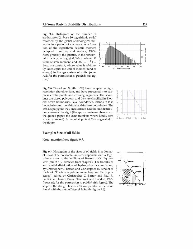
9.6 Some Basic Probability Distributions 219
Fig. 9.5. Histogram of the number ofearthquakes (in base 10 logarithmic scale)recorded by the global seismological net-works in a period of xxx years, as a func-tion of the logarithmic seismic moment(adapted from Lay and Wallace, 1995).More precisely, the quantity in the horizon-tal axis is µ = log10(M/MK) , where Mis the seismic moment, and MK = 107 J =1 erg is a constant, whose value is arbitrar-ily taken equal the unit of moment (and ofenergy) in the cgs system of units. [note:Ask for the permission to publish this fig-ure.]
23 24 25 26 27 28 29
µ = Log10(Moment/MK)
n = Log10(Number of Events)
0
1
2
3
1
10
100
1000
Number of Events
Fig. 9.6. Wessel and Smith (1996) have compiled a high-resolution shoreline data, and have processed it to sup-press erratic points and crossing segments. The shore-lines are closed polygons, and they are classified in 4 lev-els: ocean boundaries, lake boundaries, islands-in-lakeboundaries and pond-in-island-in-lake boundaries. The180,496 polygons they encountered had the size distribu-tion shown at the right (the approximate numbers are inthe quoted paper, the exact numbers where kindly sentto me by Wessel). A line of slope is -2/3 is suggested inthe figure.
0 2 4 6 8-2-4
log10(S/S0) ; S0 = 1 km2
log10(Number of Polygons)
5
4
3
2
1
0
Example: Size of oil fields
Note: mention here figure 9.7.
Fig. 9.7. Histogram of the sizes of oil fields in a domainof Texas. The horizontal axis corresponds, with a loga-rithmic scale, to the ‘millions of Barrels of Oil Equiva-lent’ (mmBOE). Extracted from chapter 2 (The fractal sizeand spatial distribution of hydrocarbon accumulation,by Christopher C. Barton and Christopher H. Scholz) ofthe book “Fractals in petroleum geology and Earth pro-cesses”, edited by Christopher C. Barton and Paul R.La Pointe, Plenum Press, New York and London, 1995.[note: ask for the permission to publish this figure]. Theslope of the straight line is -2/3, comparable to the valuefound with the data of Wessel & Smith (figure 9.6).
1
2
3
4
0

220 Appendix: Complements (very provisional)
Example: Meteorites
Note: mention here figure 9.8.
Fig. 9.8. The approximate number of mete-orites falling on Earth every year is distributedas follows: 1012 meteorites with a diameter of10−3 mm, 106 with a diameter 1 mm, 1 with adiameter 1 m, 10−4 with a diameter 100 m, and10−8 with a diameter 10 km. The statement isloosy, and I have extracted it from the generalpress. It is nevertheless clear that a log-log plotof this ‘histogram’ gives a linear trend with aslope equal to -2. Rather, transforming the di-ameter D into volume V = D3 (which is pro-portional to mass), gives the ‘histogram’ at theright, with a slope of -2/3.
log10 V/V0 (V0 = 1 m3)
-10 0 10-20
log10 (number every year)
-10
10
0
9.6.5 Spherical Distributions
The simplest probabilistic distribution over the circle and over the surfaceof the sphere are the von Mises and the Fisher probability distributions, re-spectively.
The von Mises Distribution
As already mentioned in example 6.9, and demonstrated in section 9.6.6 herebelow, the conditional volumetric probability induced over the unit circle bya 2D Gaussian is
f (θ) = k exp(
cos θ
σ2
). (9.145)
The constant k is to be fixed by the normalization condition∫ 2π
0 dθ f (θ) =1 , this giving
k =1
2 π I0(1/σ2), (9.146)
where I0( · ) is the modified Bessel function of order zero.
The Fisher Probability Distribution
Note: mention here Fisher (1953).

9.6 Some Basic Probability Distributions 221
Fig. 9.9. The circular (von Mises) distribution corre-sponds to the intersection of a 2D Gaussian by a cir-cle passing by the center of the Gaussian. Here, theunit circle has been represented, and two Gaussianswith standard deviations σ = 1 (left) and σ = 1/2(right) . In fact, this is my preferred representationof the von Mises distribution, rather than the con-ventional functional display of figure 9.10.
ϑ ϑ
Fig. 9.10. The circular (von Mises) distribution,drawn for two full periods, centered at zero, andwith values of σ equal to 2 ,
√2 , 1 , 1/
√2 , 1/2
(from smooth to sharp).
2π 3π 4π0
0
1
π
As already mentioned in example 6.9, and demonstrated in section 9.6.6here below, the conditional volumetric probability induced over the surfaceof a sphere by a 3D Gaussian is, using spherical coordinates
f (θ, ϕ) = k exp(
cos θ
σ2
). (9.147)
We can normalize this volumetric probability by∫dS(θ, ϕ)) f (θ, ϕ)) = 1 , (9.148)
with dS(θ, ϕ) = sin θ dθ dϕ . This gives
k =1
4 π χ(1/σ2), (9.149)
where
χ(x) =sinh(x)
x. (9.150)
9.6.6 Fisher from Gaussian (Demonstration)
Let us demonstrate here that the Fisher probability distribution is obtainedas the conditional of a Gaussian probability distribution over a sphere. Asthe demonstration is independent of the dimension of the space, let us takean space with n dimensions, where the (generalized) geographical coordi-nates7 are
7 The geographical coordinates (longitude and latitude) generalize much better tohigh dimensions than the more usual spherical coordinates.

222 Appendix: Complements (very provisional)
x1 = r cos λ cos λ2 cos λ3 cos λ4 . . . cos λn−2 cos λn−1
x2 = r cos λ cos λ2 cos λ3 cos λ4 . . . cos λn−2 sin λn−1
. . . = . . .
xn−2 = r cos λ cos λ2 sin λ3
xn−1 = r cos λ sin λ2
xn = r sin λ .
(9.151)
We shall consider the unit sphere at the origin, and an isotropic Gaussianprobability distribution with standard deviation σ , with its center along thexn axis, at position xn = 1 .
The Gaussian volumetric probability, when expressed as a function ofthe Cartesian coordinates is
fx(x1, . . . , xn) = k exp(− 1
2 σ2
((x1)2 + (x2)2 + · · ·+ (xn−1)2 + (xn − 1)2 )) .
(9.152)As the volumetric probability is an invariant, to express it using the geo-graphical coordinates we just need to use the replacements 9.151, to obtain
fr(r, λ, λ′, . . . ) = k exp(− 1
2 σ2
(r2 cos2λ + (r sin λ− 1)2 )) , (9.153)
i.e.,
fr(r, λ, λ′, . . . ) = k exp(− 1
2 σ2
(r2 + 1− 2 r sin λ
)). (9.154)
The condition to be on the sphere is just
r = 1 , (9.155)
so that the conditional volumetric probability, as given in equation 6.51, isjust obtained (up to a multiplicative constant) by setting r = 1 in equa-tion 9.154,
f (λ, λ′, . . . ) = k′ exp(
sin λ− 1σ2
), (9.156)
i.e., absorbing the constant exp(1/σ2) ,
f (λ, λ′, . . . ) = k′′ exp(
sin λ
σ2
). (9.157)
This volumetric probability corresponds to the n-dimensional version of theFisher distribution. Its expression is identical in all dimensions, only thenorming constant depends on the dimension of the space.

9.6 Some Basic Probability Distributions 223
9.6.7 Probability Distributions for Tensors
In this appendix we consider a symmetric second rank tensor, like the stresstensor σ of continuum mechanics.
A symmetric tensor, σij = σji , has only sex degrees of freedom, while ithas nine components. It is important, for the development that follows, toagree in a proper definition of a set of ‘independent components’. This canbe done, for instance, by defining the following six-dimensional basis forsymmetric tensors
e1 =
1 0 00 0 00 0 0
; e2 =
0 0 00 1 00 0 0
; e3 =
0 0 00 0 00 0 1
(9.158)
e4 =1√2
0 0 00 0 10 1 0
; e5 =1√2
0 0 10 0 01 0 0
; e6 =1√2
0 1 01 0 00 0 0
.
(9.159)Then, any symmetric tensor can be written as
σ = sα eα , (9.160)
and the six values sα are the six ‘independent components’ of the tensor, interms of which the tensor writes
σ =
s1 s6/√
2 s5/√
2s6/√
2 s2 s4/√
2s5/√
2 s4/√
2 s3
. (9.161)
The only natural definition of distance between two tensors is the normof their difference, so we can write
D(σ2, σ1) = ‖ σ2 − σ1 ‖ , (9.162)
where the norm of a tensor σ is8
‖ σ ‖ =√
σij σji . (9.163)
The basis in equation 9.159 is normed with respect to this norm9. In termsof the independent components in expression 9.161 the norm of a tensorsimply becomes
8 Of course, as, here, σij = σji one can also write ‖ σ ‖ =√
σij σij , but thisexpression is only valid for symmertric tensors, while the expression 9.163 is gen-erally valid.
9 It is also orthonormed, with the obvious definition of scalar product from whichthis norm derives.

224 Appendix: Complements (very provisional)
‖ σ ‖ =√
(s1)2 + (s2)2 + (s3)2 + (s4)2 + (s5)2 + (s6)2 , (9.164)
this showing that the six components sα play the role of Cartesian coordi-nates of this 6D space of tensors.
A Gaussian volumetric probability in this space has then, obviously, theform
fs(s) = k exp
(− ∑α=6
α=1(sα − sα0)2
2 ρ2
), (9.165)
or, more generally,
fs(s) = k exp(− 1
2 ρ2
(sα − sα
0)
Wαβ
(sβ − sβ
0))
. (9.166)
It is easy to find probabilistic models for tensors, when we choose ascoordinates the independent components of the tensor, as this Gaussian ex-ample suggests. But a symmetric second rank tensor may also be describedusing its three eigenvalues λ1, λ2, λ3 and the three Euler angles ψ, θ, ϕdefining the eigenvector’s directions s1 s6/
√2 s5/
√2
s6/√
2 s2 s4/√
2s5/√
2 s4/√
2 s3
= R(ψ) R(θ) R(ϕ)
λ1 0 00 λ2 00 0 λ3
R(ϕ)T R(θ)T R(ψ)T ,
(9.167)where R denotes the usual rotation matrix. Some care is required whenusing the coordinates λ1, λ2, λ3, ψ, θ, ϕ .
To write a Gaussian volumetric probability in terms on eigenvectorsand eigendirections only requires, of course, to insert in the fs(s) of equa-tion 9.166 the expression 9.167 giving the tensor components as a function ofthe eigenvectors and eigendirections (we consider volumetric probabilities—that are invariant— and not probability densities —that would require anextra multiplication by the Jacobian determinant of the transformation—),
f (λ1, λ2, λ3, ψ, θ, ϕ) = fs(s1, s2, s3, s4, s5, s6) . (9.168)
But then, of course, we still need how to integrate in the space using thesenew coordinates, in order to evaluate probabilities.
Before facing this problem, let us remark that it is the replacementin equation 9.166 of the components sα in terms of the eigenvalues andeigendirections of the tensor that shall express a Gaussian probability dis-tribution in terms of the variables λ1, λ2, λ3, ψ, θ, ϕ . Using a function thatwould ‘look Gaussian’ in the variables λ1, λ2, λ3, ψ, θ, ϕ would not corre-spond to a Gaussian probability distribution, in the sense of section 9.6.2.

9.6 Some Basic Probability Distributions 225
The Jacobian of the transformation s1, s2, s3, s4, s5, s6 λ1, λ2, λ3, ψ, θ, ϕcan be obtained using a direct computation, that gives10∣∣∣∣∂(s1, s2, s3, s4, s5, s6)
∂(λ1, λ2, λ3, ψ, θ, ϕ)
∣∣∣∣ = (λ1 − λ2) (λ2 − λ3) (λ3 − λ1) sin θ . (9.169)
The capacity elements in the two systems of coordinates are
dvs(s1, s2, s3, s4, s5, s6) = ds1 ∧ ds2 ∧ ds3 ∧ ds4 ∧ ds5 ∧ ds6
dv(λ1, λ2, λ3, ψ, θ, ϕ) = dλ1 ∧ dλ2 ∧ dλ3 ∧ dψ ∧ dθ ∧ dϕ .(9.170)
As the coordinates sα are Cartesian, the volume element of the space isnumerically identical to the capacity element,
dvs(s1, s2, s3, s4, s5, s6) = dvs(s1, s2, s3, s4, s5, s6) , (9.171)
but in the coordinates λ1, λ2, λ3, ψ, θ, ϕ the volume element and the ca-pacity are related via the Jacobian determinant in equation 9.169,
dv(λ1, λ2, λ3, ψ, θ, ϕ) = (λ1−λ2) (λ2−λ3) (λ3−λ1) sin θ dv(λ1, λ2, λ3, ψ, θ, ϕ) .(9.172)
Then, while the evaluation of a probability in the variables s1, s2, s3, s4, s5, s6should be done via
P =∫
dvs(s1, s2, s3, s4, s5, s6) fs(s1, s2, s3, s4, s5, s6)
=∫
ds1 ∧ ds2 ∧ ds3 ∧ ds4 ∧ ds5 ∧ ds6 fs(s1, s2, s3, s4, s5, s6) ,(9.173)
in the variables λ1, λ2, λ3, ψ, θ, ϕ it should be done via
P =∫
dv(λ1, λ2, λ3, ψ, θ, ϕ) f (λ1, λ2, λ3, ψ, θ, ϕ)
=∫
dλ1 ∧ dλ2 ∧ dλ3 ∧ dψ ∧ dθ ∧ dϕ ×
× (λ1 − λ2) (λ2 − λ3) (λ3 − λ1) sin θ f (λ1, λ2, λ3, ψ, θ, ϕ) .(9.174)
To conclude this appendix, we may remark that the homogeneous prob-ability distribution (defined as the one who is ‘proportional to the vol-ume distribution’) is obtained by taking both fs(s1, s2, s3, s4, s5, s6) andf (λ1, λ2, λ3, ψ, θ, ϕ) as constants.
[Note: I should explain somewhere that there is a complication when,instead of considering ‘a tensor like the stress tensor’ one consider a posi-tive tensor (like an electric permittivity tensor). The treatment above appliesapproximately to the logarithm of such a tensor.]
10 If instead of the 3 Euler angles, we take 3 rotations around the three coordinateaxes, the sin θ here above becomes replaced by the cosinus of the second angle.This is consistent with the formula by Xu and Grafarend (1997).
226 Appendix: Complements (very provisional)
9.6.8 Homogeneous Distribution of Second Rank Tensors
The usual definition of the norm of a tensor provides the only natural defi-nition of distance in the space of all possible tensors. This shows that, whenusing a Cartesian system of coordinates, the components of a tensor are the‘Cartesian coordinates’ in the 6D space of symmetric tensors. The homo-geneous distribution is then represented by a constant (nonnormalizable)probability density:
f (σxx, σyy, σzz, σxy, σyz, σzx) = k . (9.175)
Instead of using the components, we may use the three eigenvalues λ1, λ2, λ3of the tensor and the three Euler angles ψ, θ, ϕ defining the orientation ofthe eigendirections in the space. As the Jacobian of the transformation
σxx, σyy, σzz, σxy, σyz, σzx λ1, λ2, λ3, ψ, θ, ϕ (9.176)
is ∣∣∣∣∂(σxx, σyy, σzz, σxy, σyz, σzx)∂(λ1, λ2, λ3, ψ, θ, ϕ)
∣∣∣∣ = (λ1 − λ2)(λ2 − λ3)(λ3 − λ1) sin θ ,
(9.177)the homogeneous probability density 9.175 transforms into
g(λ1, λ2, λ3, ψ, θ, ϕ) = k (λ1 − λ2)(λ2 − λ3)(λ3 − λ1) sin θ . (9.178)
Although this is not obvious, this probability density is isotropic in spa-tial directions (i.e., the 3D referentials defined by the three Euler angles areisotropically distributed). In this sense, we recover ‘isotropy’ as a specialcase of ‘homogeneity’.
The rule ??, imposing that any probability density on the variablesλ1, λ2, λ3, ψ, θ, ϕ has to tend to the homogeneous probability density 9.178when the ‘dispersion parameters’ tend to infinity imposes a strong con-straint on the form of acceptable probability densities, that is, generally,overlooked.
For instance, a Gaussian model for the variables σxx, σyy, σzz, σxy, σyz, σzxis consistent (as the limit of Gaussian is a constant). This induces, via theJacobian rule, a probability density for the variables λ1, λ2, λ3, ψ, θ, ϕ , aprobability density that is not simple, but consistent. A Gaussian model forthe parameters λ1, λ2, λ3, ψ, θ, ϕ would not be consistent.
9.6.9 Center of a Probability Distribution
Let M be an n-dimensional manifold, and let P, Q, . . . represent points ofM . The manifold is assumed to have a metric defined over it, i.e., the dis-tance between any two points P and Q is defined, and denoted D(Q, P) .Of course, D(Q, P) = D(P, Q) .

9.6 Some Basic Probability Distributions 227
A normalized probability distribution P is defined over M , representedby the volumetric probability f . The probability of D ⊂ M is obtained,using the notations of equation ??, as
P(D) =∫P∈D
dv(P) f (P) . (9.179)
If ψ(P) is a scalar (invariant) function defined over M , its average valueis denoted 〈ψ 〉 , and is defined as
〈ψ 〉 ≡∫P∈M
dv(P) f (P) ψ(P) . (9.180)
This clearly corresponds to the intuitive notion of ‘average’.Let p be a real number in the range 1 ≤ p < ∞ . To any point P we can
associate the quantity (having the dimension of a length)
σp(P) =(∫
Q∈Mdv(Q) f (Q) D(Q, P)p
) 1p
. (9.181)
Definition 9.1 The point11 where σp(P) attains its minimum value is called theLp-norm center of the probability distribution f (P) , and it is denoted Pp .
Definition 9.2 The minimum value of σp(P) is called the Lp-norm radius of theprobability distribution f (P) , and it is denoted σp .
The interpretation of these definitions is simple. Take, for instance p = 1 .Comparing the two equations 9.180–9.181, we see that, for a fixed point P ,the quantity σ1(P) corresponds to the average of the distances from thepoint P to all the points. The point P that minimizes this average distanceis ‘at the center’ of the distribution (in the L1-norm sense). For p = 2 , it isthe average of the squared distances that is minimized, etc.
The following terminology shall be used:
– P1 is called the median, and σ1 is called the mean deviation;– P2 is called the barycenter (or the center, or the mean), and σ2 is called the
standard deviation (while its square is called the variance);– P∞ is called12 the circumcenter, and σ∞ is called the circumradius.
Calling P∞ and σ∞ respectively the ‘circumcenter’ and the ‘circumra-dius’ seems justified when considering, in the Euclidean plane, a volumetric
11 If there is more than one point where σp(P) attains its minimum value, any suchpoint is called a center (in the Lp-norm sense) of the probability distribution f (P) .
12 The L∞-norm center and radius are defined as the limit p → ∞ of the Lp-normcenter and radius.

228 Appendix: Complements (very provisional)
probability that is constant inside a triangle, and zero outside. The ‘circum-center’ of the probability distribution is then the circumcenter of the trian-gle, in the usual geometrical sense, and the ‘circumradius’ of the probabilitydistribution is the radius of the circumscribed circle13. More generally, thecircumcenter of a probability distribution is always at the point that mini-mizes the maximum distance to all other points, and the circumradius of theprobability distribution is this ‘minimax’ distance.
Example 9.8 Consider a one-dimensional space N , with a coordinate ω , suchthat the distance between the point ν1 and the point ν2 is
D(ν2, ν1) =∣∣∣∣ log
ν2
ν1
∣∣∣∣ . (9.182)
As suggested in XXX, the space N could be the space of musical notes, and νthe frequency of a note. Then, this distance is just (up to a multiplicative factor)the usual distance between notes, as given by the number of ‘octaves’. Consider anormalized volumetric probability f (ν) , and let us be interested in the L2-normcriteria. For p = 2 , equation 9.181 can be written
(σ2(µ)
)2 =∫ ∞
0ds(ν) f (ν)
(log
ν
µ
)2, (9.183)
The L2-norm center of the probability distribution, i.e., the value ν2 at which σ2(µ)is minimum, is easily found14 to be
ν2 = ν0 exp(∫ ∞
0ds(ν) f (ν) log
ν
ν0
), (9.184)
where ν0 is an arbitrary constant (in fact, and by virtue of the properties of the log-exp functions, the value ν2 is independent of this constant). This mean value ν2corresponds to what in statistical theory is called the ‘geometric mean’. The varianceof the distribution, i.e., the value of the expression 9.183 at its minimum, is
(σ2)2 =
∫ ∞
0ds(ν) f (ν)
(log
ν
ν2
)2. (9.185)
13 The circumscribed circle is the circle that contains the three vertices of the trian-gle. Its center (called circumcenter) is at the the point where the perpendicularbisectors of the sides cross.
14 For the minimization of the function σ2(µ) is equivalent to the minimizationof(σ2(µ)
)2 , and this gives the condition∫
ds(ν) f (ν) log(ν/µ) = 0 . For anyconstant ν0 , this is equivalent to
∫ds(ν) f (ν) (log(ν/ν0)− log(µ/ν0)) = 0 , i.e.,
log(µ/ν0) =∫
ds(ν) f (ν) log(ν/ν0) , from where the result follows. The constantν0 is necessary in these equations for reasons of physical dimensions (only thelogarithm of adimensional quantities is defined).

9.6 Some Basic Probability Distributions 229
The distance element associated to the distance in equation 9.182 is, clearly, ds(ν) =dν/ν , and the probability density associated to f (ν) is f (ν) = f (ν)/ν , so, interms of the probability density f (ν) , equation 9.184 becomes
ν2 = ν0 exp(∫ ∞
0dν f (ν) log
ν
ν0
), (9.186)
while equation 9.185 becomes
(σ2)2 =
∫ ∞
0dν f (ν)
(log
ν
ν2
)2. (9.187)
The reader shall easily verify that if instead of the variable ν , one chooses to use thelogarithmic variable ν∗ = log(ν/ν0) , where ν0 is an arbitrary constant (perhapsthe same as above), then instead of the six expressions 9.182–9.187 we would haveobtained, respectively,
s(ν∗2 , ν∗1 ) = | ν∗2 − ν∗1 |(σ2(µ∗)
)2 =∫ +∞
−∞ds(ν∗) f (ν∗) (ν∗ − µ∗)2
ν∗2 =∫ +∞
−∞ds(ν∗) f (ν∗) ν∗(
σ2)2 =
∫ +∞
−∞ds(ν∗) f (ν∗)
(ν∗ − ν∗2
)2
(9.188)
ν∗2 =∫ +∞
−∞dν∗ f (ν∗) ν∗ (9.189)
and (σ2)2 =
∫ +∞
−∞dν∗ f (ν∗)
(ν∗ − ν∗2
)2 , (9.190)
with, for this logarithmic variable, ds(ν∗) = dν∗ and f (ν∗) = f (ν∗) . The twolast expressions are the ordinary equations used to define the mean and the variancein elementary texts.
Example 9.9 Consider a one-dimensional space, with a coordinate χ , the distancebetween two poits χ1 and χ2 being denoted D(χ2, χ1) . Then, the associatedlength element is d`(χ) = D( χ + dχ , χ ) . Finally, consider a (1D) volumet-ric probability f (χ) , and let us be interested in the L1-norm case. Assume thatχ runs from a minimum value χmin to a maximum value χmax (both could beinfinite). For p = 1 , equation 9.181 can be written
σ1(χ) =∫
d`(χ′) f (χ′) D(χ′, χ) . (9.191)
230 Appendix: Complements (very provisional)
Denoting χ1 be the median, i.e., the point the point where σ1(χ) is minimum),one easily15 founds that χ1 is characterized by the property that it separates theline into two domains of equal probability, i.e.,
∫ χ1
χmin
d`(χ) f (χ) =∫ χmax
χ1
d`(χ) f (χ) , (9.192)
expression that can readily be used for an actual computation of the median, andwhich corresponds to its elementary definition. The mean deviation is then given by
σ1 =∫ χmax
χmin
d`(χ) f (χ) D(χ, χ1) . (9.193)
Example 9.10 Consider the same situation as in the previous example, but let usbecome interested in the L∞-norm case. Let χmin and χmax the minimum andthe maximum values of χ for which f (χ) 6= 0 . It can be shown that the circum-center of the probability distribution is the point χ∞ that separates the intervalχmin, χmax in two intervals of equal length, i.e., satisfying the condition
D(χ, χmin) = D(χmax, χ) , (9.194)
and that the circumradius is
σ∞ =D(χmax, χmin)
2. (9.195)
Example 9.11 Consider, in the Euclidean n-dimensional space En , with Cartesiancoordinates x = x1, . . . , xn , a normalized volumetric probability f (x) , and letus be interested in the L2-norm case. For p = 2 , equation 9.181 can be written,using obvious notations,(
σ2(y))2 =
∫dx f (x) ‖ x− y ‖2 . (9.196)
Let x2 denote the mean of the probability distribution, i.e., the point where σ2(y)is minimum (or, equivalently, where
(σ2(y)
)2 is minimum). The condition of min-imum (the vanishing of the derivatives) gives
∫dx f (x) (x− x2) = 0 , i.e.,
x2 =∫
dx f (x) x , (9.197)
which is an elementary definition of mean. The variance of the probability distribu-tion is then15 In fact, the property 9.192 of the median being intrinsic (independent of any coor-
dinate system), we can limit ourselves to demonstrate it using a special ‘Cartesian’coordinate, where d`(x) = dx , and D(x1, x2) = |x2 − x1| , where the property iseasy to demonstrate (and well known).

9.8 Physical Measurements 231
(σ2)2 =
∫dx f (x) ‖ x− x2 ‖2 . (9.198)
In the context of this example, we can define the covariance tensor
C =∫
dx f (x)(x− x2
)⊗(x− x2
). (9.199)
Note that equation 9.197 and equation 9.199 can be written, using indices, as
xi2 =
∫dx1 ∧ · · · ∧ dxn f (x1, . . . , xn) xi , (9.200)
and
Cij =∫
dx1 ∧ · · · ∧ dxn f (x1, . . . , xn) (xi − xi2) (xj − xj
2) . (9.201)
9.6.10 Dispersion of a Probability Distribution
9.7 Determinant of a Partitioned Matrix
Using well known properties of matrix algebra (e.g., Lütkepohl, 1996), thedeterminant of a partitioned matrix can be expressed as
det(
grr grsgsr gss
)= det grr det
(gss − gsr g−1
rr grs
). (9.202)
9.8 Physical Measurements
9.8.1 Operational Definitions can not be Infinitely Accurate
Note: refer here to figure 9.11, and explain that “the length” of a real ob-ject (as opposed to a mathematically defined object) can only be defined byspecifying the measuring instrument. There are different notions of lengthassociated to a given object. For instance, figure 9.11 suggests that the lengthof a piece of wood is larger when defined by the use of a calliper16 thanwhen defined by the use of a ruler17, because a calliper tends to measure thedistance between extremal points, while an observer using a ruler tends toaverage the rugosities at the wood ends.
9.8.2 The Ideal Output of a Measuring Instrument
Note: mention here figures 9.12 and 9.13.16 Calliper: an instrument for measuring diameters (as of logs or trees) consisting of
a graduated beam and at right angles to it a fixed arm and a movable arm. Fromthe Digital Webster.
17 Ruler: a smooth-edged strip (as of wood or metal) that is usu. marked off in units(as inches) and is used as a straightedge or for measuring. From the Digital Web-ster.

232 Appendix: Complements (very provisional)
Fig. 9.11. Different definitions of thelength of an object.
Fig. 9.12. Instrument built tomeasure the pitches of musi-cal notes. Due to unavoidablemeasuring noises, a measure-ment is never infinitely accu-rate. Figure 9.13 suggests anideal instrument output.
MEASURING
SYSTEM
INSTRUMENT
OUTPUT
SENSOR
Environmental
noiseInstrument
noise
9.8.3 Measurements
9.8.4 Output as Conditional Probability Density
As suggested by figure 9.14, an ‘measuring instrument’ is specified whenthe conditional volumetric probability f (y|x) for the output y , given theinput x is given.
9.8.5 A Little Bit of Theory
We want to measure a given property of an object, say the quantity x .Assume that the object has been randomly selected from a set of objects, sothat the ‘prior’ probability for the quantity x is fx(x) .
Then, the conditional. . .Then, Bayes theorem. . .
9.8.6 Example: Instrument Specification
[Note: This example is to be put somewhere, I don’t know yet where.]It is unfortunate that ordinary measuring instruments tend to just dis-
play some ‘observed value’, the ‘measurement uncertainty’ tending to behidden inside some written documentation. Awaiting the day when mea-suring instruments directly display a probability distribution for the mea-surand, let us contemplate the simple situation where the maker of an in-strument, say a frequencymeter, writes someting like the following.
This frequencymeter can operate, with high accuracy, in the range 102 Hz <ν < 109 Hz . When very far from this range, one may face uncontrollableuncertainties. Inside (or close to) this range, the measurement uncertaintyis, with a good approximation, independent of the value of the measured

9.8 Physical Measurements 233
ν = 5∗
ν = 6∗
ν = 7∗
ν = 440 Hz
ν = 220 Hz
ν = 110 Hz
ν = 880 Hz
ν = 1760 Hz
Τ = −5∗
Τ = −6∗
Τ = −7∗
ν = 100 Hz
ν = 200 Hz
ν = 300 Hz
ν = 400 Hz
ν = 500 Hz
ν = 1000 Hz
ν = 2000 Hz
Τ = 0.001 s
Τ = 0.005 s
Τ = 0.004 s
Τ = 0.002 s
Τ = 0.003 s
Τ = 0.004 s
Τ = 0.005 s
Τ = 0.01 s
ν = log ν/ν∗0
Τ = log Τ/Τ∗
0 Τ = 1/ν = 1 s00
ν = 1/Τ = 1 Hz00
ν = 440 Hz ν = +6.09∗ ∗Τ = +6.09Τ = 2.27 10 s
−3Center:
Radius (standard deviation): σ = 0.12
Fig. 9.13. The ideal output of a mesuring instrument (in this example, measuringfrequencies-periods). The curve in the middle corresponds to the volumetric prob-ability describing the information brought by the measurement (on ‘the measur-and’). Five different scales are shown (in a real instrument, the user would just selectone of the scales). Here, the logarithmic scales correspond to the natural logarithmsthat a physicist should prefer, but engineers could select scales using decimal log-arithms. Note that all the scales are ‘linear’ (with respect to the natural distance inthe frequency-period space [see section XXX]): I do not recommend the use of a scalewhere the frequencies (or the periods) would ‘look linear’.
Fig. 9.14. The input (or measurand) and the outputof a measuting instrument. The output is never anactual value, but a probability distribution, in fact,a conditional volumetric probability f (y|x) for theoutput y , given the input x .
INPUT
OUTPUT

234 Appendix: Complements (very provisional)
frequency. When the instrument displays the value ν0 , this means that the(1D) volumetric probability for the measurand is
if log νν0≤ −σ then f (ν) = 0
if − σ < log νν0
< +2 σ then f (ν) = 29 σ2
(2 σ− log ν
ν0
)if + 2 σ ≤ log ν
ν0then f (ν) = 0
,
(9.203)where σ = 10−4 . This volumetric probability is displayed at the top offigure 9.15. Using the logarithmic frequency as coordinate, this is an asym-metric triangle.
Fig. 9.15. Figure for ‘instrument specifi-cation’. Note: write this caption.
ν + 2σ∗0ν − σ∗
0
Κ = 1 Ηz
ν
Κν = log∗
10ν
0
Κν = log∗
0 10
σ = 10−4
ν = 1.0000 10 Hz0
6
ν = 6.00000
∗
ν = 6.0002
0∗
ν = 5.9999
0∗
ν = 6.0000
0∗
9.8.7 Measurements and Experimental Uncertainties
Observation of geophysical phenomena is represented by a set of parame-ters d that we usually call data. These parameters result from prior measure-ment operations, and they are typically seismic vibrations on the instrumentsite, arrival times of seismic phases, gravity or electromagnetic fields. As inany measurement, the data is determined with an associated certainty, de-scribed with a volumetric probability over the data parameter space, that wedenote here ρd(d). This density describes, not only marginals on individualdatum values, but also possible cross-relations in data uncertainties.
Although the instrumental errors are an important source of data uncer-tainties, in geophysical measurements there are other sources of uncertainty.The errors associated with the positioning of the instruments, the environ-mental noise, and the human appreciation (like for picking arrival times) arealso relevant sources of uncertainty.
Example 9.12 Non-analytic volumetric probability Assume that we wish tomeasure the time t of occurrence of some physical event. It is often assumed thatthe result of a measurement corresponds to something like

9.8 Physical Measurements 235
t = t0 ± σ . (9.204)
An obvious question is the exact meaning of the ±σ . Has the experimenter inmind that she/he is absolutely certain that the actual arrival time satisfies the strictconditions t0 − σ ≤ t ≤ t0 + σ , or has she/he in mind something like a Gaus-sian probability, or some other probability distribution (see figure 9.16)? We accept,following ISO’s recommendations (1993) that the result of any measurement hasa probabilistic interpretation, with some sources of uncertainty being analyzed us-ing statistical methods (‘type A’ uncertainties), and other sources of uncertaintybeing evaluated by other means (for instance, using Bayesian arguments) (‘type B’uncertainties). But, contrary to ISO suggestions, we do not assume that the Gaus-sian model of uncertainties should play any central role. In an extreme example, wemay well have measurements whose probabilistic description may correspond to amultimodal volumetric probability. Figure 9.17 shows a typical example for a seis-mologist: the measurement on a seismogram of the arrival time of a certain seismicwave, in the case one hesitates in the phase identification, or in the identification ofnoise and signal. In this case the volumetric probability for the arrival of the seismicphase does not have an explicit expression like f (t) = k exp(−(t− t0)2/(2σ2)) ,but is a numerically defined function. Using, for instance, the Mathematica (regis-tered trademark) computer language we may define the volumetric probability f (t)as
f[t_] := ( If[t1<t<t2,a,c] If[t3<t<t4,b,c] ) .
Here, a and b are the ‘levels’ of the two steps, and c is the ‘background’ volumetricprobability.
Fig. 9.16. What has an experi-menter in mind when she/he de-scribes the result of a measurementby something like t = t0 ± σ ? t0 t0 t0 t0
Example 9.13 The Gaussian model for uncertainties. The simplest probabilisticmodel that can be used to describe experimental uncertainties is the Gaussian model
ρD(d) = k exp(−1
2(d− dobs)T C−1
D (d− dobs))
. (9.205)
It is here assumed that we have some ‘observed data values’ dobs , with uncertain-ties described by the covariance matrix CD . If the uncertainties are uncorrelated,
ρD(d) = k exp
−12 ∑
i
(di − di
obsσi
)2 , (9.206)
where the σi are the ‘standard deviations’.

236 Appendix: Complements (very provisional)
Fig. 9.17. A seismologist tries to measure the arrival timeof a seismic wave at a seismic station, by ‘reading’ theseismogram at the top of the figure. The seismologistmay find quite likely that the arrival time of the waveis between times t3 and t4 , and believe that what isbefore t3 is just noise. But if there is a significant prob-ability that the signal between t1 and t2 is not noisebut the actual arrival of the wave, then the seismologistshould define a bimodal volumetric probability, as theone suggested at the bottom of the figure. Typically, theactual form of each peak of the volumetric probability isnot crucial (here, box-car functions are chosen), but theposition of the peaks is important. Rather than assign-ing a zero volumetric probability to the zones outsidethe two intervals, it is safer (more ‘robust’) to attributesome small ‘background’ value, as we may never ex-clude some unexpected source of error.
Time
t1 t2 t3 t4
Sign
al a
mpl
itude
t4t3t2t1
Prob
abili
ty d
ensi
ty
Time
Example 9.14 The Generalized Gaussian model for uncertainties. An alternativeto the Gaussian model, is to use the Laplacian (double exponential) model for un-certainties,
ρD(d) = k exp
(−∑
i
|di − diobs|
σi
). (9.207)
While the Gaussian model leads to least-squares related methods, this Laplacianmodel least to absolute-values methods (see section??), well known for producingrobust18 results. More generally, there is the Lp model of uncertainties
ρp(d) = k exp
(− 1
p ∑i
|di − diobs|
p
(σp)p
)(9.208)
(see figure 9.18).
-6 -4 -2 0 2 4 60
0.1
0.2
0.3
0.4
0.5
-6 -4 -2 0 2 4 60
0.1
0.2
0.3
0.4
0.5
-6 -4 -2 0 2 4 60
0.1
0.2
0.3
0.4
0.5
-6 -4 -2 0 2 4 60
0.1
0.2
0.3
0.4
0.5
-6 -4 -2 0 2 4 60
0.1
0.2
0.3
0.4
0.5
-6 -4 -2 0 2 4 60
0.1
0.2
0.3
0.4
0.5
Fig. 9.18. Generalized Gaussian for values of the parameter p = 1,√
2, 2, 4, 8 and ∞ .
18 A numerical method is called robust if it is not sensitive to a small number of largeerrors.

9.10 Parameters 237
9.9 The ‘Shipwrecked Person’ Problem
Note: this example is to be developed. For the time being this is just a copyof example 2.14
Let S represent the surface of the Earth, using geographical coordinates(longitude ϕ and latitude λ ). An estimation of the position of a floatingobject at the surface of the sea by an airplane navigator gives a probabilitydistribution for the position of the object corresponding to the (2D) volumet-ric probability f (ϕ, λ) , and an independent, simultaneous estimation of theposition by another airplane navigator gives a probability distribution cor-responding to the volumetric probability g(ϕ, λ) . How the two volumetricprobabilities f (ϕ, λ) and g(ϕ, λ) should be ‘combined’ to obtain a ‘result-ing’ volumetric probability? The answer is given by the ‘product’ of the twovolumetric probabilities densities:
( f · g)(ϕ, λ) =f (ϕ, λ) g(ϕ, λ)∫
S dS(ϕ, λ) f (ϕ, λ) g(ϕ, λ). (9.209)
9.10 Parameters
9.10.1 Parameters
To describe a physical system (a planet, an elastic sample, etc.) we use phys-ical quantities (temperature and mass density at some given points, totalmass, etc.). I examine here the situation where the quantities take real val-ues (i.e., I do not try to consider the case where the quantities take integeror complex values). The real values may have a physical dimension, length,mass, etc.
We will here that there is one very important type of quantities (calledbelow the ‘Jeffreys quantities’), and three other marginal types of quantities.
9.10.2 Jeffreys Quantities
9.10.3 Definition
Let us examine ‘positive parameters’, like a temperature, a period, etc. Oneof the properties of the parameters we have in mind is that they occur inpairs of mutually reciprocal parameters:
Period T = 1/ν ; Frequency ν = 1/TResistivity ρ = 1/σ ; Conductivity ρ = 1/σ
Temperature T = 1/(kβ) ; Thermodynamic parameter β = 1/(kT)Mass density ρ = 1/` ; Lightness ` = 1/ρ
Compressibility γ = 1/κ ; Bulk modulus (uncompressibility) κ = 1/γ .

238 Appendix: Complements (very provisional)
When physical theories are elaborated, one may freely choose one of theseparameters or its reciprocal.
Sometimes these pairs of equivalent parameters come from a definition,like when we define frequency ν as a function of the period T , by ν = 1/T .Sometimes these parameters arise when analyzing an idealized physicalsystem. For instance, Hooke’s law, relating stress σij to strain εij can beexpressed as σij = cij
k` εk` , thus introducing the stiffness tensor cijk` , or asεij = dij
k` σk` , thus introducing the compliance tensor dijk` , inverse of thestiffness tensor. Then the respective eigenvalues of these two tensors belongto the class of scalars analyzed here.
Let us take, as an example, the pair conductivity-resistivity (this may bethermal, electric, etc.). Assume we have two samples in the laboratory S1and S2 whose resistivities are respectively ρ1 and ρ2 . Correspondingly,their conductivities are σ1 = 1/ρ1 and σ2 = 1/ρ2 . How should we definethe ‘distance’ between the two samples? As we have |ρ2 − ρ1| 6= |σ2 − σ1| ,choosing one of the two expressions as the ‘distance’Awould be arbitrary.Consider the following definition of ‘distance’ between the two samples
D(S1, S2) =∣∣∣∣ log
ρ2
ρ1
∣∣∣∣ =∣∣∣∣ log
σ2
σ1
∣∣∣∣ . (9.210)
This definition (i) treats symmetrically the two equivalent parameters ρ andσ and, more importantly, (ii) has an invariance of scale (what matters is howmany ‘octaves’ we have between the two values, not the plain differencebetween the values). In fact, it is the only ‘sensible’ definition of distancebetween the two samples S1 and S2 .
Note: this is an old text. Associated to the distance D = | log (x2/x1) |is the distance element
ds = dx/x . (9.211)
Defining the reciprocal parameter y = 1/x , the same distance D, now be-comes D = | log (y2/y1) | and we have the distance element
ds = dy/y . (9.212)
Introducing the logarithmic parameters
x∗ = log(x/x0) ; y∗ = log(y/y0) , (9.213)
where x0 and y0 are arbitrary positive constants, leads to D = |x∗2 − x∗1 | =|y∗2 − y∗1 | , and to the distance elements
ds = dx∗ ; ds = dy∗ . (9.214)
Note: I have to explain here that, for all four parameters, the homogeneousvolumetric probability is a constant (that I arbitrarily take equal to one)

9.10 Parameters 239
fx(x) = 1 ; fy(y) = 1 ; fx∗(x∗) = 1 ; fy∗(y∗) = 1 . (9.215)
Should one, for some reason, choose to work with probability densities, thenwe convert volumetric probabilities into probability densities using equa-tion ?? (page ??). We then see that the same homogeneous probability distri-bution is represented by the following homogeneous probability densities:
f x(x) = 1/x ; f y(y) = 1/y ; f x∗(x∗) = 1 ; f y∗(y∗) = 1 .(9.216)
One should note that the homogeneous probability density for a Jeffreysparameter x is 1/x .
The association of the probability density f (x) = k/x to positive pa-rameters was first made by Jeffreys (1939). To honor him, we propose touse the term Jeffreys parameters for all the parameters of the type consideredabove . The 1/x probability density was advocated by Jaynes (1939), anda nontrivial use of it was made by Rietsch (1977), in the context of inverseproblems.
If we have a Jeffreys parameter x , we know that the distance elementis ds = dx/x . Defining y = xk , i.e., some power of the parameter, leads tods = (1/k), dy/y . This is, up to a multiplicative constant, the same expres-sion. Therefore, if a parameter x is a Jeffreys parameter, then, its inverse, itssquare, and, in general, any power of the parameter is also a Jeffreys param-eter.
It is important to recognize when we do not face a Jeffreys parameter.Among the many parameters used in the literature to describe an isotropiclinear elastic medium we find parameters like the Lamé’s coefficients λ andµ , the bulk modulus κ , the Poisson ratio σ , etc. A simple inspection of thetheoretical range of variation of these parameters shows that the first Laméparameter λ and the Poisson ratio σ may take negative values, so they arecertainly not Jeffreys parameters. In contrast, Hooke’s law σij = cijk` εk` ,defining a linearity between stress σij and strain εij , defines the positivedefinite stiffness tensor cijk` or, if we write εij = dijk` σk` , defines its in-verse, the compliance tensor dijk` . The two reciprocal tensors cijk` and dijk`are ‘Jeffreys tensors’. This is a notion that would take too long to develophere, but we can give the following rule: The eigenvalues of a Jeffreys tensor areJeffreys quantities.
Note: This solves the complete problem for isotropic tensors only. I haveto mention here the rules valid for general anisotropic tensors.
As the two (different) eigenvalues of the stiffness tensor cijk` are λκ = 3κ(with multiplicity 1) and λµ = 2µ (with multiplicity 5) , we see that theuncompressibility modulus κ and the shear modulus µ are Jeffreys param-eters19 (as are any parameter proportional to them, or any power of them,
19 The definition of the elastic constants was made before the tensorial structure ofthe theory was understood. Seismologists, today, should never introduce, at a the-

240 Appendix: Complements (very provisional)
including the inverses). If for some reason, instead of working with κ andµ , we wish to work with other elastic parameters, like for instance the Youngmodulus Y and the Poisson ratio σ , then the homogeneous probability dis-tribution must be found using the Jacobian of the transformation between(Y, σ) and (κ, µ) . This is done in appendix 4.1.1.
There is a problem of terminology in the Bayesian literature. The ho-mogeneous probability distribution is a very special distribution. When theproblem of selecting a ‘prior’ probability distribution arises, in the absenceof any information except the fundamental symmetries of the problem, onemay select as prior probability distribution the homogeneous distribution.But enthusiastic Bayesians do not call it ‘homogeneous’ but ‘noninforma-tive’. I do not agree with this. The homogeneous probability distribution isas informative as any other distribution, it is just the homogeneous one.
In general, each time we consider an abstract parameter space, each pointbeing represented by some parameters x = x1, x2 . . . xn , we will start bysolving the (sometimes nontrivial) problem of defining a distance betweenpoints that respects the necessary symmetries of the problem. Note: con-tinue this discussion.
9.10.4 Benford Law
Let us play a game. We randomly generate many real numbers x1, x2, . . .in the interval (e−100, e+100) , with an homogeneous probability distribution(in the elementary sense of ‘homogeneous’ for real numbers). Then we com-pute the positive quantities
X1 = ex1 ; X2 = ex2 . . . , (9.217)
write these numbers in the common way, i.e., using the base ten numberingsystem. The first digit of these numbers may then be 1, 2, 3, 4, 5, 6, 7, 8 , or9 . Which is the frequency of each of the nine digits? The answer is (note:explain here why): the frequency in which the digit n appears as first digitis
pn = log10n + 1
n. (9.218)
This means that:
oretical level, parameters like the first Lamé coefficient λ or the Poisson ratio. In-stead they should use κ and µ (and their inverses). In fact, my suggestion is touse the true eigenvalues of the stiffness tensor, λκ = 3κ , and λµ = 2µ , that Ipropose to call the eigen-bulk-modulus and the eigen-shear-modulus.
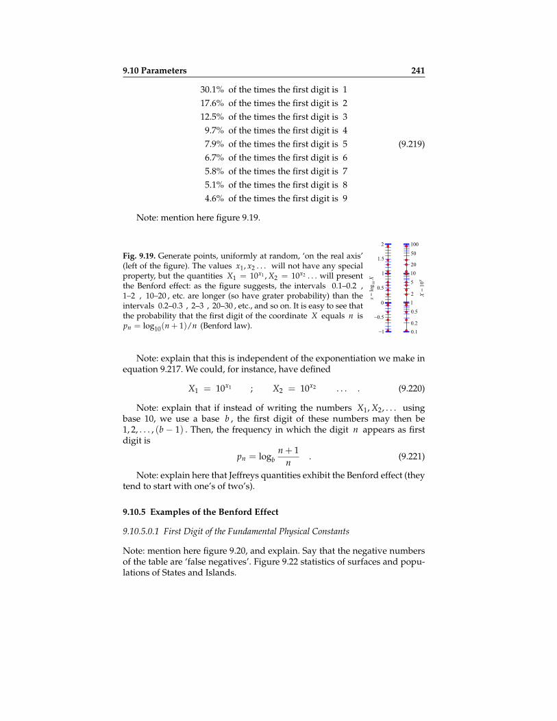
9.10 Parameters 241
30.1% of the times the first digit is 117.6% of the times the first digit is 212.5% of the times the first digit is 39.7% of the times the first digit is 47.9% of the times the first digit is 56.7% of the times the first digit is 65.8% of the times the first digit is 75.1% of the times the first digit is 84.6% of the times the first digit is 9
(9.219)
Note: mention here figure 9.19.
Fig. 9.19. Generate points, uniformly at random, ‘on the real axis’(left of the figure). The values x1, x2 . . . will not have any specialproperty, but the quantities X1 = 10x1 , X2 = 10x2 . . . will presentthe Benford effect: as the figure suggests, the intervals 0.1–0.2 ,1–2 , 10–20 , etc. are longer (so have grater probability) than theintervals 0.2–0.3 , 2–3 , 20–30 , etc., and so on. It is easy to see thatthe probability that the first digit of the coordinate X equals n ispn = log10(n + 1)/n (Benford law).
X =
10
x
0.1
1
10
100
0.2
0.5
2
5
20
50
x =
log
10 X
−1
0
1
2
−0.5
0.5
1.5
Note: explain that this is independent of the exponentiation we make inequation 9.217. We could, for instance, have defined
X1 = 10x1 ; X2 = 10x2 . . . . (9.220)
Note: explain that if instead of writing the numbers X1, X2, . . . usingbase 10, we use a base b , the first digit of these numbers may then be1, 2, . . . , (b − 1) . Then, the frequency in which the digit n appears as firstdigit is
pn = logbn + 1
n. (9.221)
Note: explain here that Jeffreys quantities exhibit the Benford effect (theytend to start with one’s of two’s).
9.10.5 Examples of the Benford Effect
9.10.5.0.1 First Digit of the Fundamental Physical Constants
Note: mention here figure 9.20, and explain. Say that the negative numbersof the table are ‘false negatives’. Figure 9.22 statistics of surfaces and popu-lations of States and Islands.

242 Appendix: Complements (very provisional)
Fig. 9.20. Statistics of the first digit inthe table of Fundamental Physical Con-stants (1998 CODATA least-squares ad-justement; Mohr and Taylor, 2001). Ihave indiscriminately taken all the con-stants of the table (263 in total). The‘model’ corresponds to the predictionthat the relative frequency of digit nin a base K system of numeration islogK(n + 1)/n . Here, K = 10 .
0
80
60
40
20
1 2 3 4 5 6 7 8 9
Actual statistics
Model
Frequency
Digits
First digit of the
Fundamental Physical Constants
(1998 CODATA least-squares adjustement)
9.10.5.0.2 First Digit of Territories and Islands
Note: mention here figures 9.21 and 9.22.
Fig. 9.21. The begining of the list of the States,Territories and Principal Islands of the World,in the Times Atlas of the World (Times Books,1983), with the first digit of the surfaces andpopulations highlighted. The statistics of thisfirst digit in shown in figure 9.22.
STATES, TERRITORIES& PRINCIPAL ISLANDSOF THE WORLDName [Plate] and Description Sq. km Sq. miles Population
Abu Dhabi, see United Arab Emirates
Afghanistan [31] 636,267 245,664 15,551,358* 1979
Capital: KabulAjman, see United Arab Emirates
Åland [51] 1,505 581 22,000 1981
Self-governing Island Territory of Finland
Albania [83] 28,748 11,097 2,590,600 1979
Capital: Tirana (Tiran )Aleutian Islands [113] 17,666 6,821 6,730* 1980
Territory of U.S.A.Algeria [88] 2,381,745 919,354 18,250,000 1979
Capital: Algiers (Alger)
American Samoa [10] 197 76 30,600 1977
Unincorporated Territory of U.S.A.
Andorra [75] 465 180 35,460 1981
Capital: Andorra la VellaAngola [91] 1,246,700 481,226 6,920,000 1981
Capital: Luanda
…
Fig. 9.22. Statistics of the first digitin the table of the surfaces (both insquared kilometers and squared miles)and populations of the States, Territo-ries and Principal Islands of the World,as printed in the first few pages ofthe Times Atlas of the World (TimesBooks, 1983). As for figure 9.20, the‘model’ corresponds to the predictionthat the relative frequency of digit n islog10(n + 1)/n .
0
400
300
200
100
1 2 3 4 5 6 7 8 9
Actual statistics
Model
Frequency
Digits
Surfaces and Populations of the States,
Territories and Principal Islands
(Times Atlas of the World)

9.11 Volumetric Histograms and Density Histograms 243
9.10.6 Cartesian Quantities
Note: explain here that a Cartesian quantity x has as finite distance the ex-pression
D = |x2 − x1| . (9.222)
Note: Explain here that most of Cartesian quantities we find in physicsare the logarithms of Jeffreys quantities.
9.10.7 Quantities ‘[0-1]’
Note: mention here the quantities x that like a chemical concentration, takevalues in the range [0, 1] . Note: explain that defining
X =x
1− x(9.223)
introduces a Jeffreys quantity (with range [0, ∞] ).
9.10.8 Ad-hoc Quantities
Note: mention here the ad-hoc quantities, like the Lamé’s parameters or thePoisson’s ratio, that we should not use.
9.11 Volumetric Histograms and Density Histograms
A volumetric probability or a probability density can be obtained as the limitof a histogram. It is important to understand which kind of histogram pro-duces as a limit a volumetric probability and which other kind of histogramproduces a probability density.
In short, when counting the number of samples inside a division of thespace into cells of equal volume one obtains a volumetric probability. If,instead, one divides the space into cells of equal capacity (i.e., in fact, onedivides the space using constant coordinate increments), one obtains a prob-ability density.
Figure 9.23 presents a one-dimensional example of the building of a his-togram. The manifold M into consideration here is a one-dimensional man-ifold where each point represents the volumetric mass ∆M/∆V of a rock.As a ‘coordinate’ over this one-dimensional manifold, we can use the valueρ = ∆M/∆V , but we could use its inverse ` = 1/ρ = ∆V/∆M as well (or,as considered below, the logarithmic volumetric mass). Let us first use thevolumetric mass ρ . To make a histogram whose limit would be a volumet-ric probability we should divide the one-dimensional manifold M into cellof equal ‘one-dimensional volume’, i.e., of equal length. This requires that adefinition of the distance between two point of the manifold is used.

244 Appendix: Complements (very provisional)
Fig. 9.23. Histograms of the volumetric mass ofthe 571 different rock types quoted by Johnsonand Olhoeft (1984). The histogram at the top,where cells with constant values of ∆ρ havebeen used, has a probability density f (ρ) aslimit. The histogram in the middle, where cellswith constant length ∆D = ∆ρ/ρ have beenused, has a volumetric probability f (ρ) aslimit. The relation between the two is f (ρ) =f (ρ)/ρ (see text for details). In reality thereis one natural variable for this problem (bot-tom), the logarithmic volumetric mass ρ∗ =log(ρ/ρ0) , as for this variable, intervals of con-stant length are also intervals with constant in-crement of the variable.
0 ρ
ρ
10 g/cm3 20 g/cm3
0 10 g/cm3 20 g/cm3
ρ∗ = log10(ρ/ρ0) ρ0 = 1 g/cm3
0.0 0.5 1.0 1.5
For reasons exposed in chapter ??, the ‘good’ definition of distance be-tween the point ρ1 and the point ρ2 is D = | log(ρ2/ρ1) | . When dividingthe manifold M into cells of constant length ∆D one obtains the histogramin the middle of figure, whose limit is a (one-dimensional) volumetric prob-ability f (ρ) .
When instead of dividing the manifold M in cells of constant length ∆Done uses cells of constant ‘coordinate increment’ ∆ρ , one obtains a differenthistogram, displayed at the top of the figure. Its limit is a probability densityf (ρ) .
The relation between the volumetric probability f (ρ) and the proba-bility density f (ρ) is that expressed in equation ??. As ∆D = log((ρ +∆ρ)/ρ) = ∆ρ/ρ + . . . , in this one-dimensional example, the equivalent ofequation ?? is
dD =1ρ
dρ . (9.224)
Therefore, equation ?? here becomes
f (ρ) = f (ρ)/ρ , (9.225)
this being the relation between the volumetric probability and the probabil-ity density obtained in figure 9.23.

9.12 Probability Density 245
The advantage of using the histogram that produces a probability den-sity is that one does not need to care about possible definitions of lengthor volume: whatever the coordinate being used, ρ , or ` = 1/ρ , one hasonly to consider constant coordinate increments, δρ , or δ` , and make thehistogram.
The advantage in using the histogram that produces a volumetric prob-ability is that, as obvious in the figure, when dividing the manifold intoconsideration in cells of equal volume (here equal length), the number ofsamples inside each cell tends to be more equilibrated, and the histogramsconverges more rapidly into significant values.
Example 9.15 Note: explain here what is a volumetric histogram and a densityhistogram. Say that while the limit of a volumetric histogram is a volumetric prob-ability, the limit of a density histogram is a probability density. Note: Introducethe notion of ‘naïve histogram’. Consider a problem where we have two physicalproperties to analyze. The first is the property of electric resistance-conductance ofa metallic wire, as it can be characterized, for instance, by its resistance R or by itsconductance 4 C = 1/R . The second is the ‘cold-warm’ property of the wire, as it canbe charcterized by its temperature T or its thermodynamic parameter β = 1/kT (kbeing the Boltzmann constant). The ‘parameter manifold’ is, here, two-dimensional.In the ‘resistance-conductance’ manifold, the distance between two points, charac-terized by the resistances R1 and R2 , or by the conductances C1 and C2 is, asexplained in section XXX,
D =∣∣∣∣log
R2
R1
∣∣∣∣ =∣∣∣∣log
C2
C1
∣∣∣∣ . (9.226)
Similarly, in the ‘cold-warm’ manifold, the distance between two points, character-ized by the temperatures T1 and T2 , or by the thermodynamic parameters β1 andβ2 is
D =∣∣∣∣log
T2
T1
∣∣∣∣ =∣∣∣∣log
β2
β1
∣∣∣∣ . (9.227)
An homogeneous probability distribution can be defined as . . . Bla, bla, bla. . . In fig-ure ??, the two histograms that can be made from the two first diagrams give thevolumetric probability. The naïve histrogram that could be made form the diagramat the right would give a probability density.
9.12 Probability Density
In this section we consider that the set Ω is, in fact, a finite-dimensionalmanifold, that we may denote M . We select for F the (THE?) Borel set ofM .
Bla, bla, and selecting some coordinates xi over the manifold, bla, bla,and Radon-Nikodym theorem, and bla, bla, and we write

246 Appendix: Complements (very provisional)
Fig. 9.24. Note: explain here how to make a volumet-ric histogram. Explain that when the electric resistanceor the temperature span orders of magnitude, some dia-grams become totally impractical.
-1 0 +1 +2 +3
+30
+40
+50
ν∗ = log10 ν/ν0
0(ν = 1 Hz)
ν∗ =
log10 ν
/ν0
Fig. 9.25. Note: write this caption.
1000 H
z
500 H
z
2 10 Hz50
0 H
z
1500 H
z
0 Hz
10 Hz50
Fig. 9.26. Note: write this caption.
0.2 0.4 0.6 0.8 1.0
0.2
0.4
0.6
1.0
0.0
0.8
0.0
FIGURE INCONSTRUCTION
P[A] =∫x1,...,xn∈A
dvx f (x1, . . . , xn) , (9.228)
where dvx = dx1 ∧ · · · ∧ dxn . Using more elementary notations,
dvx = dx1 dx2 . . . dxn , (9.229)
and equation 9.228 can be rewritten under the non manifestly covariantform
P[A] =∫x1,...,xn∈A
dx1 dx2 . . . dxn f (x1, . . . , xn) . (9.230)
The function f (x1, . . . , xn) is called the probability density (associated tothe probability distribution P and to the coordinates xi ). It is a density,in the tensorial sense of the term, i.e., under a change of variables x y itchanges according to the Jacobian rule (see below).

9.12 Probability Density 247
Example 9.16 Consider a homogeneous probability distribution at the surface ofa sphere of unit radius. When parameterizing a point by its spherical coordinates(θ, ϕ) , the associated (2D) probability density, the homogeneous probability distri-bution is represented by the function
f (θ, ϕ) =1
4πsin θ , (9.231)
and the probability of a domain A is computed as
P[A] =∫ ∫︸︷︷︸θ,ϕ∈A
dθ dϕ f (θ, ϕ) , (9.232)
the integral over the whole surface giving one.
A probability density is a density in the tensorial sense of the term. Un-der a change of variables x1, . . . , xn y1, . . . , yn , expression 9.228 be-comes
P[A] =∫y1,...,yn∈A
dvy g(y1, . . . , yn) , (9.233)
where dvy = dy1 ∧ · · · ∧ dyn . As this identity must hold for any domain A ,it must also hold infinitesimally, so we can write
dP = f (x1, . . . , xn) dx1 ∧ · · · ∧ dxn = g(y1, . . . , yn) dy1 ∧ · · · ∧ dyn .(9.234)
We have already seen that the relation between the two capacity elementsassociated to the two coordinate systems is (see equation 5.54) dy1 ∧ · · · ∧dyn = (1/X) dx1 ∧ · · · ∧ dxn , so we immediately obtain the Jacobian rule forprobability densities
g(y1, . . . , yn) = f (x1, . . . , xn) X(y1, . . . , yn) . (9.235)
Note: explain that the coordinates xi at the right take the values xi =xi(y1, . . . , yn) .
Of course, this is the general rule of transformation of scalar densities(equation 5.18, page 98), that they represent a probability density or anyother density. Note that the X appearing in this equation is the determinantof the matrix Xi
j = ∂xi/∂yj , not that of the matrix Yij = ∂yi/∂xj .
Note: I must also give the formula (referred to in the appendices)
g(y1, . . . , yn) =f (x1, . . . , xn)Y(x1, . . . , nn)
, (9.236)
and, perhaps, write it as (warning, I refer to this equation in the appendices)
248 Appendix: Complements (very provisional)
g(y) =f ( x(y) )Y( x(y) )
. (9.237)
(Note: correct what follows.) In the literature, the equivalent of equa-tion 9.235 is presented taking the absolute sign of the Jacobian determinant.In principle, we do not heed here this absolute sign, as we have assumedabove that the ‘new variables’ are always classified in a way such that theJacobian determinant is positive. It remains the case of a one-dimensionalvariable, that we may treat in an ad-hoc way20.
(Note: I must warn the reader that if there is a natural notion of volumeon the manifold, integrating densities may be quite unefficient.
Note: without a metric, we can not define the conditional probabilitydensity.
Note: without the notion of volume, we can not define the intersectionof probabilities.
9.13 Homogeneous Probability Function
Definition 9.3 Homogeneous probability. Let a volume triplet ( Ω , F , V )be given. If the volume measure of the whole set, V(Ω) , is finite, then one can in-troduce the homogeneous probability, denoted H , that, by definition, to any setA ∈ F associates a probability H[A] proportional to V[A] , the volume measureof A .
Example 9.17 If Ω is a set with a finite number of elements, say n , then thehomogenenous probability H associates, to every element ω ∈ Ω the (constant)elementary probability
p(ω) = 1/n . (9.238)
Example 9.18 If Ω is a manifold with finite volume measure V(Ω) , then thehomogenenous probability H associates, to every point P ∈ Ω the (constant)volumetric probability
f (P) = 1/V(Ω) . (9.239)
Definition 9.4 Step probability. Let a volume triplet ( Ω , F , V ) be given. Toevery subset A ∈ F with finite volume measure V[A] , we associate a probabil-ity, denoted HA , that to any A′ ∈ F associates a probability proportional to thevolume measure of A∩A′ .
Example 9.19 For a discrete probability, let k be the number of elements in A ,k = V[A] . The elementary probability associated to HA is (see figure 9.27)
p(ω) =
1/k if ω ∈ A0 if ω /∈ A .
(9.240)
20 When, for instance, passing from ρ to ` = 1/ρ , we have a negative value of theJacobian ‘determinant’, d`/dρ = −1/ρ2 .

9.13 Homogeneous Probability Function 249
Example 9.20 For a manifold, let V[A] be the volume measure of A . The volu-metric probability associated to HA is
f (P) =
1/V[A] if P ∈ A
0 if P /∈ A .(9.241)
p1A
1/4
0
00
00
1/4
1/4
1/4
Fig. 9.27. The step probability HA associated to a set A . The values of the elemen-tary probability associated to HA are proportional to the values of the indicator ofthe set A (compare this with figure 1.2).
Example 9.21 (Note: compare this with example 9.16) Consider a homogeneousprobability distribution at the surface of a sphere of unit radius. When parameter-izing a point by its spherical coordinates (θ, ϕ) , the associated (2D) volumetricprobability is
f (θ, ϕ) =1
4π. (9.242)
The probability of a domain A of the surface is computed as
P[A] =∫ ∫︸︷︷︸θϕ∈A
dS(θ, ϕ) f (θ, ϕ) , (9.243)
where dS(θ, ϕ) = sin θ dθ dϕ is the usual surface element of the sphere. The totalprobability (over the whole sphere) of course equals one.
Note: explain that the measure (or size) of a discrete set is the number ofits elements. The measure of a set A ⊆ A0 can be expressed as
M[A] = ∑a∈A
χA0(a) , (9.244)
250 Appendix: Complements (very provisional)
where χA is the indicator function associated to a set A . If the measure ofthe whole set A0 is finite, say M0 ,
M0 = M[A0] , (9.245)
then we can introduce a probability function, denoted H , that to any A ⊆A0 , associates the probability value
H[A] =M[A]M0
. (9.246)
Then,H[A] = ∑
a∈Ah(a) , (9.247)
with the elementary probability function
h(a) =χA0(a)
M0. (9.248)
If the set if a manifold, there is not “natural” measure of a set (that wouldindependent of any coordinate system), and, for this reason, we have as-sumed above the existence of a particular volume element dv . Then, themeasure (or volume) of a set A ⊆ M is
M[A] =∫P∈A
dv . (9.249)
a special definition must be introduced. This is typically done by choos-ing an arbitrary system of coordinates, and, in those coordinates, select oneparticular “volume density” (or “measure density”).
Note: rewrite this section.A probability distribution P is homogeneous if the probability asociated
by P to any domain A ⊂ M is proportional to the volume of the domain,i.e., if there is a constant k such for any A ⊂ M ,
P[A] = k V[A] . (9.250)
The homogenenous probability distribution is not necessarily normed. It fol-lows immediately from this definition that the volumetric probability f asso-ciated to the homogeneous probability distribution is constant:
f (P) = k . (9.251)
Should one not work with volumetric probabilities, but with probabilitydensities, one should realize that the probability density f associated to the ho-mogeneous probability distribution is not necessarily constant. For a probabilitydensity depends on the coordinates being used. When using a coordinate

9.15 Exercise 251
system x = xi , where the metric determinant takes the value gx(x) , theprobability density representing the homogeneous probability distributionis (using equation ??)
f x(x) = k gx(x) . (9.252)
For instance, in the physical 3D space, when using spherical coordinates,the ‘homogeneous probability density’ (this is a short name for ‘the prob-ability density representing the homogeneous probability distribution’) isf (r, θ, ϕ) = k r2 sin θ .
9.14 Popper-Bayes Algorithm
Let Mp be a p-dimensional manifold, with volume element dvp and let Mqa q-dimensional manifold, with volume element dvq . The points of Mp aredenoted P, P′ . . . , while the points of Mq are denoted Q, Q′ . . . . Let f be avolumetric probability over Mp and let ϕ be a volumetric probability overMq . Let
P 7→ Q = a(P) (9.253)
be an application from Mp into Mq . Let P be a sample point of f , andsubmit this point to a survive or perish test, the probability of survival being
π = ϕ( a(P) )/ϕmax (9.254)
(and the probability of perishing being 1−π ). If the point P perishes, then,we start again the survive or perish test with a second sample point of f ,and so on, until one point survives. Property: The surviving point is a sam-ple point of a volumetric probability h over Mp whose normalized expres-sion is
h(P) =1ν
f (P) ϕ( a(P) ) , (9.255)
the normalizing constant being ν =∫M dvp f (P) ϕ( a(P) ) . [NOTE: this is
still a conjecture, that shall be demonstrated here.]
9.15 Exercise
This exercise is all explained in the caption of figure 9.28. The exercise isthe same than that in section 9.16, excepted that while here we use sets, insection 9.16 we use volumetric probabilities. The initial intervals here (initialinformation on x and on y ) correspond to the “two-sigma” intervals of the(truncated) Gaussians of section 9.16, so the results are directly comparable.

252 Appendix: Complements (very provisional)
y = (x)
x
y
0 1 2 3 4 5 6 7
-10
0
10
20
30
40
p
q
fg
Fig. 9.28. Two quantities x and y have some definite values xtrue and ytrue , thatwe try to uncover. For the time being, we have the following information on thesetwo quantities, xtrue ∈ f = [1, 5] , and ytrue ∈ p = [14, 22] (the black intervalsin the figure). We then learn that, in fact, ytrue = ϕ(xtrue) , with the function x 7→y = ϕ(x) = x2 − (x − 3)3 represented above. To deduce the “posterior” intervalcontaining xtrue , we can first introduce the reciprocal image ϕ-1(p) of the intervalp (blue interval at the bottom), then define the intersection g = f ∩ ϕ-1(p) (redinterval at the bottom). To obtain the “posterior” interval containing ytrue , we canjust evaluate the image of the interval g by the mapping: q = ϕ(g) = ϕ( f ∩ ϕ-1(p)) .We could have obtained the interval q following a different route. We could firsthave evaluated the image of f , to obtain the interval ϕ( f ) (blue interval at the left).The intersection of the interval p with the interval ϕ( f ) then gives the same intervalq , because of the property ϕ( f ∩ ϕ-1(p)) = ϕ( f )∩ p .
9.16 Exercise
This exercise is all explained in the caption of figure 9.29. The exercise is thesame than that in section 9.15, excepted that while here we use volumetricprobabilities, in section 9.15 we use sets. The initial (truncated) Gaussianshere (initial information on x and on y ) are such that the “two-sigma” in-tervals of the Gaussians correspond to the intervals defining the sets in sec-tion 9.15. Therefore, the results are directly comparable.

9.16 Exercise 253
y = (x)
x
y
0 1 2 3 4 5 6 7
-10
0
10
20
30
40
p(y)
q(y)
f(x)
g(x)
Fig. 9.29. Two quantities x and y have some definite values xtrue and ytrue , thatwe try to uncover. For the time being, we have some (independent) informationon these two quantities, represented by the volumetric probabilities f (x) and p(y)(black functions in the figure). We then learn that, in fact, ytrue = ϕ(xtrue) , with thefunction x 7→ y = ϕ(x) = x2 − (x − 3)3 represented at the top-right. To obtainthe volumetric probability representing the “posterior” information on xtrue thereis only the following way. The volumetric probability p(y) is transported from theordinate to the abscissa axis, by application of the notion of preimage of a volumetricprobability. This gives the volumetric probability [ϕ-1(p)](x) , by application of theformula ??. This function is represented in blue (dashed line) at the bottom of thefigure. The volumetric probability representing the posterior information on xtrue isthen obtained by the intersection of f (x) and of [ϕ-1(p)](x) , using formula ??. Thisgives the function g(x) represented in red at the bottom. In total, then, we have eval-uated g = f ∩ ϕ-1(p) . To obtain the “posterior” information on ytrue we just trans-port the g(x) just obtained from the abscissa into the ordinate axis, i.e., we computethe image p = ϕ(g) of g using formula ??. This gives the function q(y) representedin red at the left of the figure. We then have q = ϕ(g) = ϕ( f ∩ ϕ-1(p)) . We couldhave arrived at q(y) following a different route. We could first have evaluated theimage of f (x) , to obtain the function [ϕ( f )](y) , represented in blue (dashed line) atthe left. The intersection of p(y) with [ϕ( f )](y) then gives the same q(y) , because,as demonstrated in the text, ϕ( f ∩ ϕ-1(p)) = ϕ( f )∩ p . Note: the original functionsf (x) and p(y) were two Gaussians (respectively centered at x = 3 and y = 18 ,and with standard deviations σx = 1 and σy = 2 ), truncated inside the workingintervals x ∈ [−1/2 , 7 ] and y ∈ [ ϕ(−1, 2) , ϕ(7) ] .


10 Appendix: Inverse Problems (very provisional)
10.1 Inverse Problems
10.1.1 Inverse Problems
[Note: Complete and expands what follows.]In the so called ‘inverse problems’, values of the parameters describ-
ing physical systems are estimated, using as data some indirect measure-ments. A consistent formulation of inverse problems can be made using theconcepts of probability theory. Data and attached uncertainties, (a possiblyvague) a priori information on model parameters, and a physical theory re-lating the model parameters to the observations are the fundamental ele-ments of any inverse problem. While the most general solution of the inverseproblem requires extensive use of Monte Carlo methods, special hypothesis(e.g., Gaussian uncertainties) allow, in some cases, to solve part of the prob-lem analytically (e.g., using the method of least squares).
Given a physical system, the ‘forward’ of ‘direct’ problem consists, bydefinition, in using a physical theory to predict the outcome of possible ex-periments. In classical physics, this problem has a unique solution. For in-stance, given a seismic model of the whole Earth (elastic constants, attenu-ation, etc. at every point inside the Earth) and given a model of a seismicsource, we can use current seismological theories to predict which seismo-grams should be observed at given locations at the Earth’s surface.
The ‘inverse problem’ arises when we do not have a good model of theEarth, or a good model of the seismic source, but we have a set of seismo-grams, and we wish to use these observations to infer the internal Earthstructure or a model of the source (typically we try to infer both).
There are many reasons that make the inverse problem underdetermined(the solution is not unique). In the seismic example, two different Earthmodels may predict the same seismograms1, the finite bandwidth of ourdata sets will never allow us to resolve very small features of the Earthmodel, and there are always experimental uncertainties that allow differentmodels to be ‘acceptable’.
1 For instance, we could fit our observations with a heterogeneous but isotropicEarth model or, alternatively, with an homogeneous but anisotropic Earth.

256 Appendix: Inverse Problems (very provisional)
The name ‘inverse problem’ is widely accepted. I only like this namemoderately, as I see the problem more as a problem of ‘conjunction of statesof information’ (theoretical, experimental and a priori information). In fact,the equations used below have a range of applicability well beyond ‘inverseproblems’: they can be used, for instance, to predict the values of observa-tion in a realistic situation where the parameters describing the Earth modelare not ‘given’, but only known approximately.
In fact, I like to think of an ‘inverse’ problem as merely a ‘measurement’.A measurement that can be quite complex, but the basic principles and thebasic equations to be used are the same for a relatively complex ‘inverseproblem’ as for a relatively simple ‘measurement’.
10.1.2 Model Parameters and Observable Parameters
Although the separation of all the variables of a problem in two groups maysometimes be artificial, we take this point of view here, since it allows us topropose a simple setting for a wide class of problems.
We may have in mind a given physical system, like the whole Earth, ora small crystal under our microscope. The system (or a given state of thesystem) may be described by assigning values to a given set of parametersm = m1, m2, . . . , mNM that we will name the model parameters.
Let us assume that we make observations on this system. Although weare interested in the parameters m , they may not be directly observable, sowe may make some indirect measurement like obtaining seismograms at theEarth’s surface for analyzing the Earth’s interior, or making spectroscopicmeasurements for analyzing the chemical properties of a crystal. The set ofobservable parameters will be represented by o = o1, o2, . . . , oNO .
We assume that we have a physical theory that solves the forward problem,i.e., that given an arbitrary model m , it allows us to predict the theoreticaldata values o that an ideal measurement should produce (if m was the ac-tual system). The generally nonlinear function that associates to any modelm the theoretical data values o may be represented by a notation like
oi = oi(m1, m2, . . . , mNM) ; i = 1, 2, . . . , ND , (10.1)
or, for short,o = o(m) . (10.2)
In fact, it is this expression that separates the whole set of our parametersinto the subsets o and m , as sometimes there is no difference of naturebetween the parameters in o and the parameters in m . For instance, inthe classical inverse problem of estimating the hypocenter coordinates ofan earthquake, we may put in o the arrival times of the seismic wavesat some seismic observatories, and we need to put in m the coordinatesof the observatories —as these are parameters that are needed to computethe travel times—, although we estimate arrival times of waves as well ascoordinates of the observatories using similar types of measurements.

10.1 Inverse Problems 257
10.1.3 A Priori Information on Model Parameters
In a typical geophysical problem, the model parameters contain geometricalparameters (positions and sizes of geological bodies) and physical parame-ters (values of the mass density, of the elastic parameters, the temperature,the porosity, etc.).
The a priori information on these parameters is all the information we pos-sess independently of the particular measurements that will be consideredas ‘data’ (to be described below). This probability distribution is, generally,quite complex, as the model space may be high dimensional, and the pa-rameters may have nonstandard probability densities.
To this, generally complex, probability distribution over the model spacecorresponds a volumetric probability that we denote as ρprior(m) .
If an explicit expression for the volumetric probability ρprior(m) isknown, then it can be used in analytical developments. But such an explicitexpression is, by no means, necessary. All that is needed is a set of proba-bilistic rules that allows us to generate samples of ρprior(m) in the modelspace (random samples distributed according to ρprior(m) ).
Example 10.1 Gaussian a priori Information.Of course, the simplest example of a probability distribution is the Gaussian
(or ‘normal’) distribution. Not many physical parameters accept the Gaussian asa probabilistic model (we have, in particular, seen that many positive parametersare Jeffreys parameters, for which the simplest consistent volumetric probability isnot the normal, but the lognormal). But if we have chosen the right parameters (forinstance, taking the logarithms of all Jeffreys parameters), it may happen that theGaussian probabilistic model is acceptable. We then have
ρprior(m) = k exp(−1
2(m−mprior)T M-1
prior (m−mprior))
. (10.3)
When this Gaussian volumetric probability is used, mprior , the center of the Gaus-sian is called the ‘a priori model’ while Mprior is called the ‘a priori covariance ma-trix’. The name ‘a priori model’ is dangerous, as for large dimensional problems, theaverage model may not be a good representative of the models that can be obtainedas samples of the distribution (see figure 10.11 as an example). Other usual sourcesof prior information are the ranges and distribution of media properties in the rocks,or probabilities for the localization of media discontinuities. If the information refersto marginals of the model parameters, and is not including the description of rela-tions across model parameters, the prior volumetric probability reduces to a productof univariate volumetric probabilities. The next example illustrates this case.
Example 10.2 Prior Information for a 1D Mass Density ModelWe consider the problem of describing a model consisting of a stack of horizontal
layers with variable thickness and uniform mass density. The prior information isshown in figure 10.1, involving marginal distributions of the mass density and the

258 Appendix: Inverse Problems (very provisional)
layer thickness. Spatial statistical homogeneity is assumed, hence marginals are notdependent on depth in this example. Additionally, they are independent of neighborlayer parameters. The model parameters consist of a sequence of thicknesses and asequence of mass density parameters, m = `1, `2, . . . , `NL, ρ1, ρ2, . . . , ρNL . Themarginal prior probability densities for the layer thicknesses are all assumed to beidentical and of the form (exponential volumetric probability)
f (`) =1`0
exp(− `
`0
), (10.4)
where the constant `0 has the value `0 = 4 km (see the left of figure 10.1), whileall the marginal prior probability densities for the mass density are also assumed tobe identical, and of the form (lognormal volumetric probability)
g(ρ) =1√
2π σexp
(− 1
2 σ2
(log
ρ
ρ0
)2)
, (10.5)
where ρ0 = 3.98 g/cm3 and σ = 0.58 (see the right of figure 10.1). Assumingthat the probability distribution of any layer thickness is independent of the thick-nesses of the other layers, that the probability distribution of any mass density isindependent of the mass densities of the other layers, and that layer thicknesses areindependent of mass densities, the a priori volumetric probability in this problemis the product of a priori probability densities (equations 10.4 and 10.5) for eachparameter,
ρprior(m) = ρm(`1, `2, . . . , `NL, ρ1, ρ2, . . . , ρNL) = kNL
∏i
f (ρi) g(ρi) .
(10.6)Figure 10.2 shows (pseudo) random models generated according to this probabilitydistribution. Of course, the explicit expression 10.6 has not been used to generatethese random models. Rather, consecutive layer thicknesses and consecutive massdensities have been generated using the univariate probability densities defined byequations 10.4 and 10.5.
Fig. 10.1. At left, the probability den-sity for the layer thickness. At right, theprobability density for the density ofmass. 0 5 10 15 20 25 30
0
0.05
0.1
0.15
0.2
0.25
0 5 10 15 20 250
0.2
0.4
0.6
0.8
1
Mass Density (g/cm3)Depth (km)
Example 10.3 Geostatistical Modeling[Note: I must give here as an example the use of a priori information in
geophysical inverse problems the geostatistics approach, as developed, for

10.1 Inverse Problems 259
Fig. 10.2. Three random Earth models gener-ated according to the a priori probability den-sity in the model space.
020
40
60
80
100
0 5
10
15
20
020
40
60
80
100
0 5
10
15
20
020
40
60
80
100
0 5
10
15
20
100
80
60
40
20
0
100
80
60
40
20
0
100
80
60
40
20
0
20151050 2 015105020151050
Dep
th (
km)
Mass Density (g/cm3)
instance, by Journel and Huijbregts (1978). I may also mention the inversestratigraphic modeling of Bornholdt et al. (1999) and of Cross and Lessenger(1999).]
10.1.4 Modeling Problem (or Forward Problem)
Physics analyzes the correlations existing between physical parameters. Instandard mathematical physics, these correlations are represented by ‘equal-ities’ between physical parameters (like when we write f = m a to relate theforce f applied to a particle, the mass m of the particle and the accelerationa ). In the context of inverse problems this corresponds to assuming that wehave a function from the ‘parameter space’ to the ‘data space’ that we mayrepresent as
o = o(m) . (10.7)
We do not mean that the relation is necessarily explicit. Given m , we mayneed to solve a complex system of equations in order to get o , but this,nevertheless, defines a function m → o = o(m) .
10.1.5 Measurements and Experimental Uncertainties
Note: the text that was here has been moved to section 9.8.7. Remember thatwe end here with a volumetric probability σobs(o) , that represents the resultof our measurements.
10.1.6 Combination of Available Information
10.1.7 Solution in the Model Parameter Space
The basic idea is easy to explain when imagining a Monte Carlo approach,that can be defined without the need of an explicit expression for the finalresult. Then, our task is to find the analytic expression corresponding to thisMonte Carlo approach.
The data of the problem are as follows:
– a volumetric probability on the model parameter space M ,
ρprior(m) , (10.8)
representing the a priori information we have on the model parameters;

260 Appendix: Inverse Problems (very provisional)
– a mapping from M into O ,
m 7→ o = o(m) , (10.9)
providing the solution of the modeling problem (or ‘forward’ problem);– and a volumetric probability in the observable parameters manifold O ,
σobs(o) , (10.10)
representing the information on the observable parameters obtainedfrom some observations (or ‘measurements’).
The approach about to be proposed2 is not the shorter nor the more el-egant. But it has the advantage of corresponding to the more general of allthe possible implementations. The justification of the proposed approach isobtained in section 10.1.8, where the link is made with the notion of con-junction of states of information.
Basic Monte Carlo Approach: We consider, in M , a "very large" set ofpoints, that is sample of ρprior(m) . For each point m of the sample, wecompute the predicted values of the observable parameters, o(m) . A ran-dom decision is taken to keep the model m or to discard it, the probabilityfor the model m to be kept being
π = σobs( o(m) )/σmaxobs , (10.11)
i.e., the probability is proportional to the value of the volumetric probabilityσobs(o) at the point o(m) . The subset of models (of the initial set) that havebeen kept define a volumetric probability, that we denote ρpost(m) , and thatwe call the posterior volumetric probability.
To obtain the expression for ρpost(m) , we only need to remark that thissituation is exactly that examined in section ??. Therefore, the solution foundthere applies here: the posterior volumetric probability just defined can beexpressed as
ρpost(m) =1ν
ρprior(m) σobs( o(m) ) , (10.12)
where ν is the normalizing constant
ν =∫
Mdvm ρprior(m) σobs( o(m) ) . (10.13)
2 In some of my past writings, I have introduced inverse problems using the notionof conditional volumetric probability (or conditional probability density). The def-initions are then different, and lead to different, more complex solutions (see, forinstance, Mosegaard and Tarantola, 2002). The approach proposed here replacesthe old one.

10.1 Inverse Problems 261
Example 10.4 Gaussian model. When the model parameter manifold and the ob-servable parameter manifold are linear spaces, the Gaussian model for uncertaintiesmay apply:
σobs(o) =1
(2π)n/2√
det Oobs
exp(
- 12 (o− oobs)t O -1
obs (o− oobs))
ρprior(m) =1
(2π)n/2√
det Mprior
exp(
- 12 (m−mprior)t M -1
prior (m−mprior))
.
(10.14)
Note: explain here the meaning of oobs (the ‘observed values’ of the observablepatrameters), Oobs , mprior , and Mprior . Then,
ρpost(m) =1ν
exp( - S(m) ) , (10.15)
where the misfit function S(m) is the sum of squares defined through
2 S(m) = ( o(m)− oobs )t O-1obs ( o(m)− oobs )
+ ( m−mprior )t M-1prior ( m−mprior ) ,
(10.16)
and where ν is the normalizing constant ν =∫M dvm(m) exp( - S(m) ) . The
maximum likelihood model is the model maximizing ρpost(m) , i.e., the model min-imizing S(m) . For that reason, one may call it the ‘best model in the least-squaressense’.
Example 10.5 Gaussian linear model. If the relation between model parametersand data parameters is linear, there is a matrix Ω such that
o = o(m) = Ω m . (10.17)
Then, the posterior probability density ρpost(m) is also Gaussian with mean
mpost = ( Ωt O-1obs Ω + M-1
prior )-1 ( Ωt O-1obs oobs + M-1
prior mprior )
= mprior + ( Ωt O-1obs Ω + M-1
prior )-1 Ωt O-1obs ( oobs −Ω mprior )
= mprior + Mprior Ωt ( Ω Mprior Ωt + Oobs )-1 (oobs −Ω mprior)(10.18)
and covariance
Mpost = ( Ωt O-1obs Ω + M-1
prior )-1
= Mprior −Mprior Ωt ( Ω Mprior Ωt + Oobs )-1 Ω Mprior .
(10.19)

262 Appendix: Inverse Problems (very provisional)
Example 10.6 If, in the previous example, there is, in fact, no a priori informationon the model parameters, we an formally take Mprior → ∞ I , and the first ofequations 10.18 reduces to
mpost = ( Ωt O-1obs Ω )-1 Ωt O-1
obs oobs , (10.20)
while the first of equations 10.19 gives
Mpost = ( Ωt O-1obs Ω)-1 . (10.21)
Example 10.7 If, in the previous example, the number of model parameters equalsthe number of observable parameters, and the matrix Ω is invertible, then one has
mpost = Ω-1 oobs , (10.22)
an equation that corresponds to the Kramer solution of a linear system. The posteriorcovariance matrix can be written
Mpost = Ω-1 Oobs Ω-t . (10.23)
10.1.8 Solution in the Observable Parameter Space
We here raise a series of questions that, although apparently innocent, re-quire intricate developments.
– Given the a priori information on the model parameters, as representedby the volumetric probability ρprior(m) , and given the theoretical map-ping m 7→ o = o(m) , which is the (probabilistic) prediction we canmake for the observable parameters o ? In other words, which is thevolumetric probability σprior(o) obtained in the observable parametermanifold by transport, via m 7→ o(m) , of the prior volumetric probabil-ity ρprior(m) ?
– Which is the volumetric probability σpost(o) obtained by transport ofthe posterior volumetric probability ρpost(m) ?
– How are related the two volumetric probabilities σprior(o) and σpost(o) ?
We can anticipate the answer to the last question (that is demonstrated be-low). The relation is
σpost(o) =1ν
σprior(o) σobs(o) . (10.24)
where ν is the same normalizing constant obtained above (equations 10.12–10.13). This is a very important expression. It demonstrates that the proce-dure we have used to define the solution of an inverse problem is consistentwith the product of volumetric probabilities in the observable parametersmanifold: the posterior distribution for the observable parameters equals

10.1 Inverse Problems 263
the product of the prior distribution by the distribution describing the mea-surements. It is this internal consistency of the theory that gives weight tothe definition of the solution of an inverse problem via the ‘Monte Carloparadigm’ used above.
The starting point for the development is to consider the model parame-ter manifold M , on which the model parameters mα can be considered ascoordinates. There also is the observable parameters manifold O , in whichthe observable parameters oi can be considered coordinates. Both mani-folds are assumed to be metric, with respective metric tensors gm and go .Note, in particular, that the manifold O is assumed to exist, and to have ametric, independently of the existence of M . The relation o = o(m) definesan application from M into O .
As M and O have different dimension, the kind of considered map-ping matters. Let us start by assuming that there are “more data than un-knowns”, i.e., where the number of observable parameters oi is largerthan the number of model parameters mα . Denoting p = dim(M) andq = dim(O) , we then have p ≤ q ). This situation is represented in fig-ure 10.3.
Fig. 10.3. This representation corre-sponds to the case when there is onemodel parameter m and two observ-able parameters o1, o2 (case p <q ).
ρprior(m)
m
o1
m
o2
σprior(o)o=o(m)
So, in the case now examined ( dim(M) ≤ dim(O) ), the mapping o =o(m) defines in the manifold O a subspace of dimension dim(M) : theimage of M by the application o = o(m) , that we may denote as o(M) .As suggested in figure 10.3, the coordinates mα , that are coordinates ofM , can also be used as coordinates over the g(M) .
Our question is: which volumetric probability τ(o) is induced on Oby the volumetric probability ρprior(m) over M and the application m 7→o = o(m) ? It is obvious that there is one, and that it is unambiguouslydefined. For a sample of ρprior(m) can be transported to O via the mappingo = o(m) , where it will become, by definition, a sample of the transportedprobability distribution.
The expression of the induced volumetric probability, say σprior(o) , hasbeen obtained in equation ??. It satisfies the relation
σprior( o(m) ) = ρprior(m)√
det gm(m)√det( Ωt(m) go(o(m)) Ω(m) )
,
(10.25)

264 Appendix: Inverse Problems (very provisional)
where Ω is the matrix of partial derivatives Ωiα = ∂oi/∂mα . Note that this
expression does not explicitly gives a function of o (note: explain this).We know that the volumetric probability σprior(o) is singular, as it is
only nonzero inside the submanifold of o(M) ⊂ O that is of dimensiondim(M) . This (singular) volumetric probability σprior(o) is to be be inte-grated with the volume element induced over o(M) by the metric go , thatis (see equation ??)
dωp =√
det( Ωt(m) go(o(m)) Ω(m) ) dm1 ∧ · · · ∧ dmp . (10.26)
(remember that we are using the coordinates mα over o(M) ).This ends the problem of ‘prior data prediction’, i.e., the problem of
transporting ρprior(m) from M into O . The transport of ρpost(m) is donein the same way, so one obtains an expression similar to 10.25, but this timeconcerning the posterior distributions:
σpost( o(m) ) = ρpost(m)√
det gm(m)√det( Ωt(m) go(o(m)) Ω(m) )
. (10.27)
Inserting here equation 10.12 one obtains
σpost( o(m) ) =1ν
ρprior(m) σobs( o(m) )√
det gm(m)√det( Ωt(m) go(o(m)) Ω(m) )
,
(10.28)i.e., using expression 10.25, σpost( o(m) ) = 1
ν σprior( o(m) ) σobs( o(m) ) .Denoting o(m) by o , this can be written
σpost(o) =1ν
σprior(o) σobs(o) , (10.29)
that is the result we had anticipated in equation 10.24.
Example 10.8 Note: demonstrate here that in the linear Gaussian case (exam-ple 10.5, page 261), σprior(o) is a Gaussian centered at oprior = Ω mprior withcovariance matrix Oprior = Ω Mprior Ωt , while σpost(o) is a Gaussian centeredat opost = Ω mpost with covariance matrix Opost = Ω Mpost Ωt . Explain thatin the case being here analyzed ( p ≤ q ), the q× q matrices Oprior and Opost canonly be regular if p = q .
It remains to analyze the case when p ≥ q (see figure 10.4). Which is,in the case p ≥ q the volumetric probability σprior(o) induced in O by theprior volumetric probability ρprior(m) and the mapping o(m) ?
The result is obtained by a direct application of equation ??. We mustfirst separate the p model parameters into two subsets,

10.1 Inverse Problems 265
Fig. 10.4. Same as in figure 10.3, but in thecase p > q .
o1
o2
σprior(o)ρprior(m)
m1
m2
m3
o=o(m)
m1, . . . , mq, mq+1, . . . , mp = µ1, . . . , µq, νq+1, . . . νp , (10.30)
i.e., for short,m = µ, ν . (10.31)
We must then rewrite the application m 7→ o = o(m) as
µ, ν 7→ o = o(µ, ν) , (10.32)
and solve a q× q system for the model parameters µ :
µ = µ(o, ν) . (10.33)
Then, in terms of probability densities (see equation ??)
σprior(o) =∫
dνq+1 ∧ · · · ∧ dνpρprior(µ, ν)
| det Ω(µ, ν) | , (10.34)
where Ω is the q× q matrix of partial derivatives Ωiα = ∂oi/∂mα . In the
right-hand side of equation 10.34 it is understood that the two occurrencesof µ have to be replaced by the function of o and ν obtained above (equa-tion 10.33).
Denoting by gm(m) the metric tensor in the model parameter manifold,and by go(o) the metric tensor in the observable parameter manifold, wecan transform equation 10.34 into an equation concerning volumetric prob-abilities:
σprior(o) =1√
det go(o)
∫dνq+1 ∧ · · · ∧ dνp
√det gm(µ, ν)
| det Ω(µ, ν) | ρprior(µ, ν) .
(10.35)This solves the problem of ‘prior data prediction’ in the case p ≥ q .
For the transportation of ρpost(m) from M into O , one can followexactly the same approach as for the case p ≤ q , to obtain σpost(o) =1ν σprior(o) σobs(o) , i.e., equation 10.24 again. So we see that this equationis also valid in the case p ≥ q .
Example 10.9 Note: I have to revisit here example 10.8, in the case p ≥ q .

266 Appendix: Inverse Problems (very provisional)
i . >
/ , . : ' -
F h L . : I r
I w - i
l . -
l . 1 . + < l '
I i -.12
i .
. ' ! " ,i
I r _
, ' . \
?I
i . . ) " 7
1- . r f - l
l * - '. , . , \ - + " \ \
r . . - " - , _ . l ' ' i .
' ' " ' j -
',ft-..,
rI J . t r + u >
. b/" t -- -
l a n l ' a ) z a q
-r- ( [ \ ! , ; , l - ]
] v l " c ' i
J L* - ; ' ' " -+-: : t : U ; J L /
( : ) l ' (2
( , - . n c ^ n ' )
- - ( 2 q
\,?; ' ' -2 ' .Y. ' - - Q-
Fig. 10.5. Scan.

10.1 Inverse Problems 267
1,1 . .2 r , ,. lI
I *I
( r . : : " ^ - , ) - ) ! - t
" - I . l ^ t l
t - l
Fig. 10.6. Scan.
10.1.9 Implementation of Inverse Problems
Once the volumetric probability ρpost(m) has been defined, there are dif-ferent ways of ‘using’ it.
If the model parameter manifold M has a small number of dimensions(say between one and four), the values of ρpost(m) can be computed atevery point of a grid and a graphical representation of ρpost(m) can beattempted. A visual inspection of such a representation is usually worth athousand ‘estimators’ (central estimators or estimators of dispersion). But,of course, if the values of ρpost(m) are known at all significant points, theseestimators can also be computed. This point of view is emphasized in sec-tion XXX. If the ‘model space’ M has a large number of dimensions (sayfrom five to many millions or billions), then an exhaustive exploration of thespace is not possible, and we must turn to Monte Carlo sampling methodsto extract information from ρpost(m) . We discuss the application of MonteCarlo methods to inverse problems in 10.1.11. Finally, the optimization tech-niques are discussed in section 10.1.14.
10.1.10 Direct use of the Volumetric Probability
Note: write this section.
10.1.11 Using Monte Carlo Methods
[Note: Write a small introduction here].

268 Appendix: Inverse Problems (very provisional)
10.1.12 Sampling the Prior Probability Distribution
The first step in the Monte Carlo analysis is to switch off the comparisonbetween computed and observed data, thereby generating samples of thea priori probability density. This allows us verify statistically that the algo-rithm is working correctly, and it allows us to understand the prior informa-tion we are using. We will refer to a large collection of models representingthe prior probability distribution as the “prior movie”. The more modelspresent in this movie, the more accurate representation of the prior proba-bility density.
If we are interested in smooth Earth models (knowing, e.g., that onlysmooth properties are resolved by the data), a smooth movie can be pro-duced simply by smoothing the individual models of the original movie.
10.1.13 Sampling the Posterior Probability Distribution
If we now switch on the comparison between computed and observed datausing, e.g., the Metropolis Rule, the random walk sampling the prior dis-tribution is modified into a walk sampling the posterior distribution. Again,smoothed versions of this “posterior movie” can be generated by smoothingthe individual models in the original, posterior movie.
Since data rarely put strong constraints on The Earth, the “posteriormovie” typically shows that many different models are possible. But eventhough the models in the posterior movie may be quite different, all of thempredict data that, within experimental uncertainties, are models with highlikelihood. In other words, we must accept that data alone cannot have apreferred model.
The posterior movie allows us to perform a proper resolution analysisthat helps us to choose between different interpretations of a given data set.Using the movie we can answer complicated questions about the correla-tions between several model parameters. To answer such questions, we canview the posterior movie and try to discover structure that is well resolvedby data. Such structure will appear as “persistent” in the posterior movie.Another, more traditional, way of investigating resolution is to calculate co-variances and higher order moments.
Note: continue the discussion.
10.1.14 Appendix: Using Optimization Methods
As we have seen, the solution of an inverse problem essentially consists of aprobability distribution over the space of all possible models of the physicalsystem under study. In general, this ‘model space’ is highly-dimensional,and the only general way to explore it is by using the Monte Carlo methodsdeveloped in section ??.

10.1 Inverse Problems 269
If the probability distributions are ‘bell-shaped’ (i.e., if they look like aGaussian or like a generalized Gaussian), then, one may simplify the prob-lem by calculating only the point around which the probability is maximum,with an approximate estimation of the variances and covariances. This is theproblem addressed in this section. [Note: I rephrased this sentence] Amongthe many methods available to obtain the point at which a scalar func-tion reaches its maximum value (relaxation methods, linear programmingtechniques, etc.), we limit our scope here to the methods using the gradi-ent of the function, which we assume can be computed analytically or, atleast, numerically. For more general methods, the reader may have a look atFletcher, (1980, 1981), Powell (1981), Scales (1985), Tarantola (1987), or Scaleset al. (1992).
10.1.15 Maximum Likelihood Point
Let us consider a space X , with a notion of volume element dV defined.If some coordinates x ≡ x1, x2, . . . , xn are chosen over the space, thevolume element has an expression dV(x) = v(x) dx , and each probabilitydistribution over X can be represented by a probability density f (x) . Forany fixed small volume ∆V , we can search for the point xML such thatthe probability dP of the small volume, when centered around xML , getsa maximum. In the limit ∆V → 0 this defines the maximum likelihood point.The maximum likelihood point may be unique (if the probability distribu-tion is monomodal), may be degenerated (if the probability distribution is‘roof-shaped’) or may be multiple (as when we have the sum of a few bell-shaped functions).
The maximum likelihood point is not the point at which the probabilitydensity is maximum. [Note: Rephrase the following sentence...] For our def-inition imposes that what must be maximum is the ratio of the probabilitydensity by the function v(x) defining the volume element:
x = xML ⇐⇒ F(x) =f (x)v(x)
maximum . (10.36)
We recognize in the ratio F(x) = f (x)/v(x) the volumetric probability as-sociated to the probability density f (x) (see equation ??). As the homoge-neous probability density is µ(x) = k v(x) (see rule ??), we can equivalentlydefine the maximum likelihhod point by the condition
x = xML ⇐⇒ f (x)µ(x)
maximum . (10.37)
The point at which a probability density has its maximum is not xML .In fact, the maximum of a probability density does not correspond to an in-trinsic definition of a point: a change of coordinates x 7→ y = ψ(x) would

270 Appendix: Inverse Problems (very provisional)
change the probability density f (x) into the probability density g(y) (ob-tained using the Jacobian rule), but the point of the space at which f (x) ismaximum is not the same as the point of the space where g(y) is maximum(unless the change of variables is linear). This contrasts with the maximumlikelihood point, as defined by equation 10.37, that is an intrinsically definedpoint: no matter which coordinates we use in the computation we alwaysobtain the same point of the space.
10.1.16 Misfit
One of the goals here is to develop gradient-based methods for obtainingthe maximum of F(x) = f (x)/µ(x) . As a quite general rule, gradient-basedmethods perform quite poorly for (bell-shaped) probability distributions, aswhen one is far from the maximum the probability densities tend to be quiteflat, and it is difficult to get, reliably, the direction of steepest ascent. Takinga logarithm transforms a bell-shaped distribution into a paraboloid-shapeddistribution on which gradient methods work well.
The logarithmic volumetric probability, or misfit, is defined as S(x) =− log(F(x)/F0) , where p′ and F0 are two constants, and is given by
S(x) = − logf (x)µ(x)
. (10.38)
The problem of maximization of the (typically) bell-shaped function f (x)/µ(x)has been transformed into the problem of minimization of the (typically)paraboloid-shaped function S(x) :
x = xML ⇐⇒ S(x) minimum . (10.39)
Example 10.10 The conjunction σ(x) of two probability densities ρ(x) andϑ(x) was defined (equation ??) as
σ(x) = pρ(x) ϑ(x)
µ(x). (10.40)
Then,S(x) = Sρ(x) + Sϑ(x) , (10.41)
where
Sρ(x) = − logρ(x)µ(x)
; Sϑ(x) = − logϑ(x)µ(x)
. (10.42)
Example 10.11 In the context of Gaussian distributions, we have found the prob-ability density (see example ??)
ρpost(m) = (10.43)

10.1 Inverse Problems 271
= k exp(−1
2
((m−mprior)t M-1
prior (m−mprior) + (o(m)− oobs)t O-1obs (o(m)− oobs)
)).
The limit of this distribution for infinite variances is a constant, so in this caseµm(m) = k . The misfit function S(m) = − log( ρpost(m)/µm(m) ) is thengiven by
2 S(m) = (m−mprior)t M-1prior (m−mprior)+ (o(m)−oobs)t O-1
obs (o(m)−oobs) .(10.44)
The reader should remember that this misfit function is valid only for weakly non-linear problems (see examples ?? and ??). The maximum likelihood model here is theone that minimizes the sum of squares 10.44. This correpponds to the least squarescriterion.
Example 10.12 In the context of Laplacian distributions, we have found the prob-ability density (see example ??)
ρpost(m) = k exp
(−(
∑α
|mα −mαprior|
σα+ ∑
i
| f i(m)− oiobs|
σi
)).
(10.45)The limit of this distribution for infinite mean deviations is a constant, so hereµm(m) = k . The misfit function S(m) = − log( ρpost(m)/µm(m) ) is thengiven by
S(m) = ∑α
|mα −mαprior|
σα+ ∑
i
| f i(m)− oiobs|
σi. (10.46)
The reader should remember that this misfit function is valid only for weakly non-linear problems. The maximum likelihood model here is the one that minimizes thesum of least absolute values 10.46. This correpponds to the least absolute valuescriterion.
10.1.17 Gradient and Direction of Steepest Ascent
One must not consider as synonymous the notions of ‘gradient’ and ‘direc-tion of steepest ascent’. Consider, for instance, an adimensional misfit func-tion3 S(P, T) over a pressure P and a temperature T . Any sensible defi-nition of the gradient of S will lead to an expression like
grad S =
∂S∂P
∂S∂T
(10.47)
and this by no means can be regarded as a ‘direction’ in the (P, T) space (forinstance, the components of this ‘vector’ does not have the dimensions ofpressure and temperature, but of inverse pressure and inverse temperature).
3 We take this example because typical misfit functions are adimensional, but theargument has general validity.

272 Appendix: Inverse Problems (very provisional)
Mathematically speaking, the gradient of a function S(x) at a point x0is the linear application that is tangent to S(x) at x0 . [Note: Rephrase thefollowing sentence...] This definition of gradient is consistent with the moreelementary one, based on the use of the first order development
S(x0 + δx) = S(x0) + γT0 δx + . . . (10.48)
Here, it is γ0 what is called the gradient of S(x) at point x0 . It is clear thatS(x0) + γT
0 δx is a linear application, and that it is tangent to S(x) at x0 , sothe two defintions are, in fact, equivalent. Explicitly, the components of thegradient at point x0 are
(γ0)p =∂S∂xp (x0) . (10.49)
Everybody is well trained at computing the gradient of a function (eventif the interpretation of the result as a direction in the original space is wrong).How can we pass from the gradient to the direction of steepest ascent (abona fide direction in the original space)? In fact, the gradient (at a givenpoint) of a function defined over a given space E ) is an element of the dualof the space. To obtain a direction in E , we must pass from the dual to theprimal space. As usual, it is the metric of the space that maps the dual of thespace into the space itself. So if g is the metric of the space where S(x) isdefined, and if γ is the gradient of S at a given point, the direction of steepestascent is
γ = g-1 γ . (10.50)
The direction of steepest ascent must be interpreted as follows: if we areat a point x of the space, we can consider a very small hypersphere aroundx0 . The direction of steepest ascent points towards the point of the sphereat which S(x) gets its maximum value.
Example 10.13 Figure 10.7 represents the level lines of a scalar function S(u, v)in a 2D space. A particular point has been selected. What is the gradient of thefunction at the given point? As suggested in the main text, it is not an arrow ‘per-pendicular’ to the level lines of the function at the considered point, as the notionof perpendicularity will depend on a metric not yet specified (and unnecessary todefine the gradient). The gradient must be seen as ‘the linear function that is tan-gent to S(u, v) at the considered point’. If S(u, v) has been represented by itslevel lines, then the gradient may also be represented by its level lines (right of thefigure). We see that the condition, in fact, is that the level lines of the gradient aretangent to the level lines of the original function (at the considered point). Contraryto the notion of perpendicularity, the notion of tangency is metric-independent.
Example 10.14 In the context of least squares, we consider a misfit function S(m)and a covariance matrix OM . If γ0 is the gradient of S , at a point x0 , and if weuse OM to define distances in the space, the direction of steepest ascent is
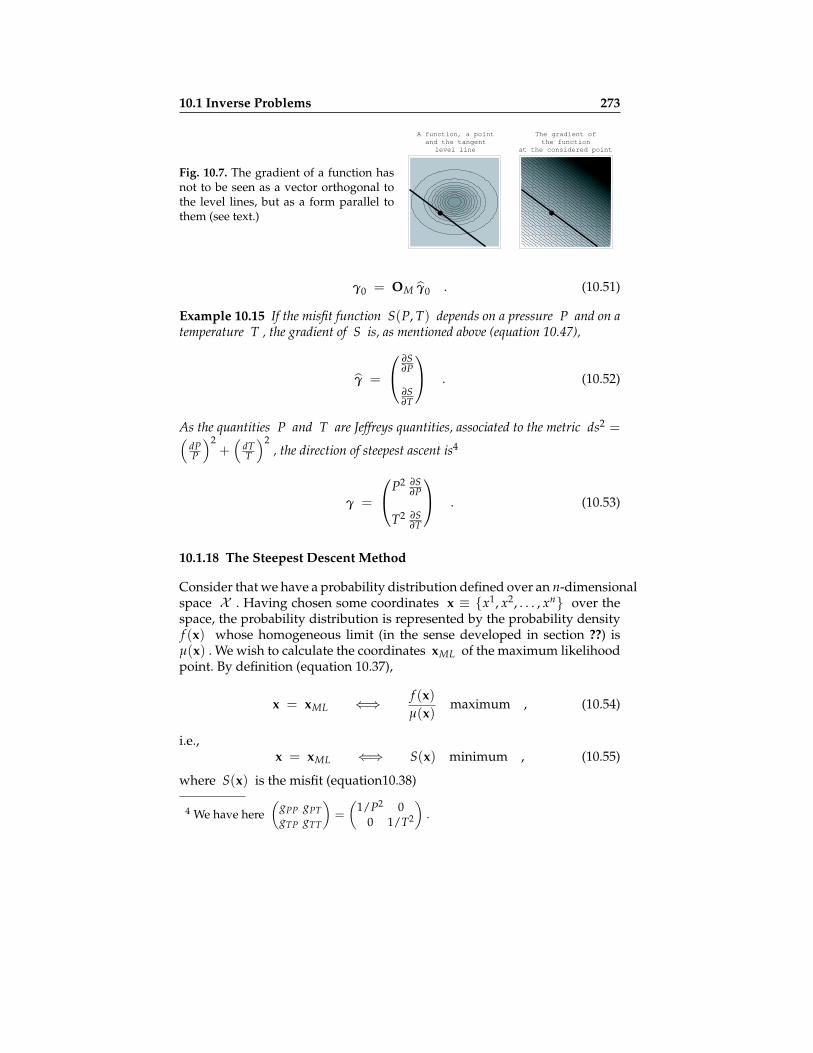
10.1 Inverse Problems 273
Fig. 10.7. The gradient of a function hasnot to be seen as a vector orthogonal tothe level lines, but as a form parallel tothem (see text.)
A function, a pointand the tangent
level line
The gradient ofthe function
at the considered point
γ0 = OM γ0 . (10.51)
Example 10.15 If the misfit function S(P, T) depends on a pressure P and on atemperature T , the gradient of S is, as mentioned above (equation 10.47),
γ =
∂S∂P
∂S∂T
. (10.52)
As the quantities P and T are Jeffreys quantities, associated to the metric ds2 =(dPP
)2+(
dTT
)2, the direction of steepest ascent is4
γ =
P2 ∂S∂P
T2 ∂S∂T
. (10.53)
10.1.18 The Steepest Descent Method
Consider that we have a probability distribution defined over an n-dimensionalspace X . Having chosen some coordinates x ≡ x1, x2, . . . , xn over thespace, the probability distribution is represented by the probability densityf (x) whose homogeneous limit (in the sense developed in section ??) isµ(x) . We wish to calculate the coordinates xML of the maximum likelihoodpoint. By definition (equation 10.37),
x = xML ⇐⇒ f (x)µ(x)
maximum , (10.54)
i.e.,x = xML ⇐⇒ S(x) minimum , (10.55)
where S(x) is the misfit (equation10.38)
4 We have here(
gPP gPTgTP gTT
)=(
1/P2 00 1/T2
).

274 Appendix: Inverse Problems (very provisional)
S(x) = −k logf (x)µ(x)
. (10.56)
Let us denote by γ(xk) the gradient of S(x) at point xk , i.e. (equa-tion 10.49),
(γ0)p =∂S∂xp (x0) . (10.57)
We have seen above that γ(x) is not to be interpreted as a direction in thespace X , but a direction in the dual space. The gradient can be convertedinto a direction using some metric g(x) over X . In simple situations themetric g will be that used to define the volume element of the space, i.e.,we will have µ(x) = k v(x) = k
√det g(x) , but this is not a necessity,
and iterative algorithms may be accelerated by astute introduction of ad-hoc metrics.
Given, then, the gradient γ(xk) (at some particular point xk ) to anypossible choice of metric g(x) we can define the direction of steepest ascentassociated to the metric g , by (equation 10.51)
γ(xk) = g-1(xk) γ(xk) . (10.58)
The algorithm of steepest descent is an iterative algorithm passing frompoint xk to point xk+1 by making a ‘small jump’ along the local directionof steepest descent,
xk+1 = xk − εk g-1k γk , (10.59)
where εk is an ad-hoc (real, positive) value adjusted to force the algorithmto converge rapidly (if εk is chosen too small the convergence may be tooslow; it is it chosen too large, the algorithm may even diverge).
Many elementary presentations of the steepest descent algorithm justforget to include the metric gk in expression 10.59. These algorithms are notconsistent. Even the physical dimensionality of the equation is not assured.The authors of this article have traced some ‘numerical’ problems in existingcomputer implementations of steepest descent algorithms to this neglectionof the metric.
Example 10.16 In the context of example 10.11, where the misfit function S(m)is given by
2 S(m) = (o(m)−oobs)t O-1obs (o(m)−oobs)+ (m−mprior)t M-1
prior (m−mprior) ,(10.60)
the gradient γ , whose components are γα = ∂S/∂mα , is given by the expression
γ(m) = Ft(m) O-1obs (o(m)− oobs) + M-1
prior (m−mprior) , (10.61)
where F is the matrix of partial derivatives

10.1 Inverse Problems 275
Fiα =∂ f i
∂mα. (10.62)
An example of computation of partial derivatives is given in appendix ??.
Example 10.17 In the context of example 10.16 the model space M has an obvi-ous metric, namely that defined by the inverse of the ‘a priori’covariance operatorg = M-1
prior . Using this metric and the gradient given by equation 10.61, the steep-est descent algorithm 10.59 becomes
mk+1 = mk − εk
(Mprior Ft
k O-1obs (fk − oobs) + (mk −mprior)
), (10.63)
where Fk ≡ F(mk) and fk ≡ f(mk) . The real positive quantities εk can befixed, after some trial and error, by accurate linear search, or by using a linearizedapproximation5.
Example 10.18 In the context of example 10.16 the model space M has a lessobvious metric, namely that defined by the inverse of the ‘a posteriori’ covarianceoperator, g = M-1
post . Note: Explain here that the ‘best current estimator’ of Mpostis
Mpost ≈(
Ftk O-1
obs Fk + M-1prior
)-1. (10.64)
Using this metric and the gradient given by equation 10.61, the steepest descentalgorithm 10.59 becomes
mk+1 = mk− εk
(Ft
k O-1obs Fk + M-1
prior
)-1 (Ft
k O-1obs (fk − oobs) + M-1
prior (mk −mprior))
,(10.65)
where Fk ≡ F(mk) and fk ≡ f(mk) . The real positive quantities εk can befixed, after some trial and error, by accurate linear search, or by using a linearizedapproximation that simply gives6 εk ≈ 1 .
The algorithm 10.65 is usually called a ‘quasi-Newton algorithm’. [Note:Rephrase the following sentence...] This is a misname, as a Newton methodapplied to the minimization of the misfit function S(m) would be a methodusing the second derivatives of S(m) , and thus the derivatives Hi
αβ =∂2 f i
∂mα∂mβ , that are not computed (or not estimated) when using this algorithm.It is just a steepest descent algorithm with a nontrivial definition of metricin the working space. In this sense it belongs to the wider class of ‘variablemetric methods’, not discussed in this article.
5 As shown in Tarantola (1987), if γk is the direction of steepest ascent at pointmk , i.e., γk = Mprior Ft
k O-1obs (fk − oobs) + (mk −mprior) , then, a local linearized
approximation for the optimal εk gives εk =γt
k M-1prior γk
γtk( Ft
k O-1obs Fk+M-1
prior) γk.
6 While a sensible estimation of the optimal values of the real positive quantitiesεk is crucial for the algorithm 10.63, they can, in many usual circumstances, bedropped from the algorithm 10.65.

276 Appendix: Inverse Problems (very provisional)
Example 10.19 In the context of example 10.12, where the misfit function S(m)is given by
S(m) = ∑i
| f i(m)− oiobs|
σi+ ∑
α
|mα −mαprior|
σα, (10.66)
the gradient γ whose components are γα = ∂S/∂mα is given by the expression
γα = ∑i
Fiα 1σi
sign( f i − oiobs) +
1σα
sign(mα −mαprior) , (10.67)
where Fiα = ∂ f i∂/mα . We can now choose in the model space the ad-hoc metricdefined as the inverse of the ‘covariance matrix’ formed by the square of the meandeviations σi and σα (interpreted as if they were variances). Using this metric,the direction of steepest ascent associated to the gradient in 10.67, is
γα = ∑i
Fiα σi sign( f i − oiobs) + σα sign(mα −mα
prior) . (10.68)
The steepest descent algorithm can now be appplied:
mk+1 = mk − εkγk . (10.69)
The real positive quantities εk can be fixed after some trial and error or by accuratelinear search.
An expression like 10.66 defines a sort of deformed polyhedron, and tosolve this sort of minimization problems the linear programming techniquesare often advocated (e.g., Claerbout and Muir, 1973). We have found that forproblems involving many dimensions the crude steepest descent methoddefined by equations 10.68–10.69 performs extremely well. For instance, inDjikpéssé and Tarantola (1999) a large-sized problem of waveform fittingis solved using this algorithm. It is well known that the sum of absolutevalues 10.66 provides a more robust7 criterion than the sum of squares 10.60.If one fears that the data set to be used is corrupted by some unexpectederrors, the least-absolute values criterion should be preferred to the leastsquares criterion8.
7 A method is ‘robust’ if its output is not sensible to a small number of large errorsin the inputs.
8 Of course, it would be much better to develop a realistic model of the uncertain-ties, and use the more general probabilistic methods developed above, but if thosemodels are not available, then the least absolute values criterion is a valuable cri-terion.

10.1 Inverse Problems 277
10.1.19 Estimation of A Posteriori Uncertainties
In the Gaussian context, the Gaussian probability density that is tangent toρpost(m) has its center at the point given by the iterative algorithm
mk+1 = mk − εk
(Mprior Ft
k O-1obs (fk − oobs) + (mk −mprior)
), (10.70)
(equation 10.63) or, equivalently, by the iterative algorithm
mk+1 = mk− εk
(Ft
k O-1obs Fk + M-1
prior
)-1 (Ft
k O-1obs (fk − oobs) + M-1
prior (mk −mprior))
(10.71)(equation 10.65). The covariance of the tangent gaussian is
Mpost ≈(
Ft∞ O-1
obs F∞ + M-1prior
)-1, (10.72)
where F∞ refers to the value of the matrix of partial derivatives at theconvergence point.
[note: Emphasize here the importance of Mpost ].
10.1.20 Some Comments on the Use of Deterministic Methods
10.1.20.0.3 About the Use of the Term ‘Matrix’
[note: Warning, old text to be updated.] Contrary to the next chapter, wherethe model parameter space and the data space may be functional spaces, Iassume here that we have discrete spaces, with a finite number of dimen-sions. [Note: What is ’indicial’ ?] Then, it makes sense to use the indicialnotation
o = oi , i ∈ ID ; m = mα , i ∈ IM , (10.73)
where ID and IM are two index sets, for the data and the model pa-rameters respectively. In the simplest case, the indices are simple integers,ID = 1, 2, 3 . . . , and IM = 1, 2, 3 . . . , but this is not necessarily true.For instance, figure 10.8 suggests a 2D problem where we compute the grav-itational field from a distribution of masses. Then, the index α is betterunderstood as consisting on a pair of integers.
10.1.20.0.4 Linear, Weakly Nonlinear and Nonlinear Problems
There are different degrees of nonlinearity. Figure 10.9 illustrates the fourdomains of nonlinearity allowing the use of the different optimisation al-gorithms This figure symbolically represents the model space in the ab-scissa axis, and the data space in the ordinates axis. The gray oval represents

278 Appendix: Inverse Problems (very provisional)
Fig. 10.8. A simple example where theindex in m = mα is not necessar-ily an integer. In this case, where we areinterested in predicting the gravitationalfield g generated by a 2-D distributionof mass, the index α is better understoodas consisting on a pair of integers. Here,for instance, mA,B means the total massin the block at row A and column B .
m3,4
m2,4
m1,4
m3,3
m2,3
m1,3
m3,2
m2,2
m1,2
m3,1
m2,1
m1,1g1
g4
g3
g2
the information coming in part from a priori information on the model pa-rameters and coming in part from the data observations9. It is the functionρ(o, m) = σobs(o) ρprior(m) seen elsewhere (note: say where).
Fig. 10.9. Illustration of thefour domains of nonlinearityallowing the use of the differ-ent optimization algorithmsThe model space is symbol-ically represented in the ab-scissa axis, and the data spacein the ordinates axis. Thegray oval represents the infor-mation coming in part froma priori information on themodel parameters and com-ing in part from the data ob-servations. What is importantis not some intrinsic nonlin-earity of the function relat-ing model parameters to data,but how linear the function isinside the domain of significantprobabilty.
M
D
dobs
mpriorM
D
dobs
mprior
d = g(m)
d = g(m)
σΜ(m) σΜ(m)
M
D
dobs
mprior
d = G mσΜ(m)
M
D
dobs
mprior
d = g(m)
d - dprior = G0 (m - mprior)
σΜ(m)
Linear problem Linearisable problem
Non-linear problemWeakly non-linear problem
To fix ideas, the oval suggests here a Gaussian probability, but the sortingof problems we are about to make as a function of their nonlinearity will notdepend fundamentally on this.
9 The gray oval is the product of the probability density over the model space,representing the a priori information, times the probability density over the dataspace representing the experimental results.
10.1 Inverse Problems 279
First, there are some strictly linear problems. For instance, in the exampleillustrated by figure 10.8, the gravitational field g depends linearly on themasses inside the blocks10
Strictly linear problems are illustrated at the top left of figure 10.9. Thelinear relationship between data and model parameters, o = Ω m , is repre-sented by a straight line. The a priori probability density ρ(o, m) “induces”,on this straight line, the a posteriori probability density (warning: this no-tation corresponds to volumetric probabilities) σ(o, m) whose “projection”over the model space gives gives the a posteriori probability density overthe model parameter space, ρpost(m) . Should the a priori probability den-sities be Gaussian, then the a posteriori probability distribution would alsobe Gaussian: this is the simplest situation (in such problems, as we will latersee (section xxx), the problem reduces to find the mean and the covarianceof the a posteriori Gaussian).
Quasi-linear problems are illustrated at the bottom-left of figure 10.9. Ifthe relationship linking the observable data o to the model parameters m ,
o = o(m) , (10.74)
is approximately linear inside the domain of significant a priori probability (i.e.,inside the gray oval of the figure), then the a posteriori probability is assimple as the a priori probability. For instance, if the a priori probability isGaussian the a posteriori probability is also Gaussian.
In this case also, the problem can be reduced to the computation of themean and the covariance of the Gaussian. Typically, one begins at some“starting model” m0 (typically, one takes for m0 the “a priori model”mprior ) (note: explain clearly somewhere in this section that “a priori model”is a language abuse for the “mean a priori model”), linearizing the functiono = o(m) around m0 and one looks for a model m1 “better than m0 ”.
Iterating such an algorithm, one tends to the model m∞ at which the“quasi-Gaussian” ρpost(m) is maximum. The linearizations made in order
10 The gravitational field at point x0 generated by a distribution of volumetric massρ(x) is given by
g(x0) =∫
dV(y)x0 − y‖x0 − x‖3 ρ(x) .
When the volumetric mass is constant inside some predefined (2-D) volumes, assuggested in figure 10.8, this gives
g(x0) = ∑A
∑B
GA,B(x0) mA,B .
This is a strictly linear equation between data (the gravitational field at a givenobservation point) and the model parameters (the masses inside the volumes).Note that if instead of choosing as model parameters the total masses inside somepredefined volumes one chooses the geometrical parameters defining the sizes ofthe volumes, then the gravity field is not a linear function of the parameters. Moredetails can be found in Tarantola and Valette (1982b, page 229).

280 Appendix: Inverse Problems (very provisional)
to arrive to m∞ are not, so far, an approximation: the point m∞ is perfectlydefined independently of any linearization, and any method used to find it.But once the convergence to this point has been obtained, a linearization ofthe function o = o(m) around this point,
o− o(m∞) = Ω∞ (m−m∞) , (10.75)
allows to obtain a good approximation of the a posteriori uncertainties. Forinstance, if the a priori probability is Gaussian this will give the covarianceof the “tangent Gaussian”.
Between linear and quasi-linear problem there are the “linearizable prob-lems”. The scheme at the top-right of figure 10.9 shows the case where thelinearization of the function o = o(m) around the a priori model,
o− g(mprior) = Ωprior (m−mprior) , (10.76)
gives a function that, inside the domain of significant probability, is verysimilar to the true (nonlinear) function.
In this case, there is no practical difference between this problem andthe strictly linear problem, and the iterative procedure necessary for quasi-linear problems is here superfluous.
It remains to analyze the true nonlinear problems that, using a pleonasm,are sometimes called strongly nonlinear problems. They are illustrated at thebottom-right of figure 10.9.
In this case, even if the a priori probability is simple, the a posterioriprobability can be quite complicated. For instance, it can be multimodal.[Note: Rephrase the following sentence...] These problems are, in general,quite complex to solve, and only the Monte Carlo methods described in theprevious chapter are sufficiently general.
If full Monte Carlo methods cannot be used, because they are too ex-pensive, then one can mix some random part (for instance, to choose thestarting point) and some deterministic part. The optimization methods ap-plicable to quasi-linear problems can, for instance, allow us to go from therandomly chosen starting point to the “nearest” optimal point (note: explainthis better). Repeating these computations for different starting points onecan arrive at a good idea of the a posteriori probability in the model space.
10.1.20.0.5 The Maximum Likelihood Model
The most likely model is, by definition, that at which the volumetric probabil-ity σβ(m) attains its maximum. As σβ(m) is maximum when S(m) isminimum, we see that the most likely model is also the the ‘best model’ ob-tained when using a ‘least squares criterion’. Should we have used the dou-ble exponential model for all the uncertainties, then the most likely modelwould be defined by a ‘least absolute values’ criterion.
There are many circumstances where the most likely model is not aninteresting model. One trivial example is when the volumetric probability

10.1 Inverse Problems 281
has a ‘narrow maximum’, with small total probability (see figure 10.10). Amuch less trivial situation arises when the number of parameters is verylarge, as for instance when we deal with a random function (that, in all rigor,corresponds to an infinite number of random variables). Figure XXX, forinstance, shows a few realizations of a Gaussian function with zero meanand an (approximately) exponential correlation. The most likely function isthe center of the Gaussian, i.e., the null function shown at the left. But thisis not a representative sample (specimen) of the probability distribution, asany realization of the probability distribution will have, with a probabilityvery close to one, the ‘oscillating’ characteristics of the three samples shownat the right.
Fig. 10.10. One of the circumstances where the‘maximum likelihood model’ may not be veryinteresting, is when it corresponds to a narrowmaximum, with small total probability, as thepeak at the left of this probability distribution.
-40 -20 0 20 400
0.2
0.4
0.6
0.8
1
10.1.20.0.6 The Interpretation of ‘The Least Squares Solution’
Note: explain here that when working with a large number of dimensions,the center of a Gaussian is a bad representer of the possible realizations ofthe Gaussian.
Mention somewhere that mpost is not the ‘posterior model’, but the cen-ter of the a posteriori Gaussian, and explain that for multidimensional prob-lems, the center of a Gaussian is not representative of a random realisationof the Gaussian.
[note: Mention somewhere that one should not compute the inverse ofthe matrices, but solve the associated linear system.]
Fig. 10.11. At the right, three random realizations of a Gaussian random functionwith zero mean and (approximatelty) exponential correlation function. The mostlikely function, i.e., the center of the Gaussian, is shown at the left. We see that themost likely function is not a representative of the probability distribution.


Bibliography
Aki, K., and Richards, P.G., 1980, Quantitative seismology, (2 volumes), Free-man and Co.
Andresen, B., Hoffmann, K. H., Mosegaard, K., Nulton, J. D., Pedersen, J. M.,and Salamon, P., On lumped models for thermodynamic properties ofsimulated annealing problems, Journal de Physique, 49, 1485–1492, 1988.
Backus, G., 1970a. Inference from inadequate and inaccurate data: I, Pro-ceedings of the National Academy of Sciences, 65, 1, 1-105.
Backus, G., 1970b. Inference from inadequate and inaccurate data: II, Pro-ceedings of the National Academy of Sciences, 65, 2, 281-287.
Backus, G., 1970c. Inference from inadequate and inaccurate data: III, Pro-ceedings of the National Academy of Sciences, 67, 1, 282-289.
Backus, G., 1971. Inference from inadequate and inaccurate data, Mathemat-ical problems in the Geophysical Sciences: Lecture in applied mathe-matics, 14, American Mathematical Society, Providence, Rhode Island.
Backus, G., and Gilbert, F., 1967. Numerical applications of a formalism forgeophysical inverse problems, Geophys. J. R. astron. Soc., 13, 247-276.
Backus, G., and Gilbert, F., 1968. The resolving power of gross Earth data,Geophys. J. R. astron. Soc., 16, 169-205.
Backus, G., and Gilbert, F., 1970. Uniqueness in the inversion of inaccurategross Earth data, Philos. Trans. R. Soc. London, 266, 123-192.
Ben-Menahem, A., and Singh, S.J., 1981. Seismic waves and sources, SpringerVerlag.
Bender, C.M., and Orszag, S.A., 1978. Advanced mathematical methods forscientists and engineers, McGraw-Hill.
Borel, É., 1967, Probabilités, erreurs, 14e éd., Paris.Borel, É., dir., 1924–1952, Traité du calcul des probabilités et de ses applica-
tions, 4 t., Gauthier Villars, Paris.Bourbaki, N., 1970, Éléments de mathématique, Hermann.Cantor, G., 1884, Über unendliche, lineare Punktmannigfaltigkeiten, Ar-
beiten zur Mengenlehre aus dem Jahren 1872-1884. Leipzig, Teubner.Choquet-Bruhat, Y., and C. DeWitt-Morette, 1982, Analysis, manifolds, and
physics, North-Holland.Claerbout, J.F., and Muir, F., 1973. Robust modelling with erratic data, Geo-
physics, 38, 5, 826-844.

284 Appendix: Inverse Problems (very provisional)
Dahl-Jensen, D., Mosegaard, K., Gundestrup, N., Clow, G. D., Johnsen, S. J.,Hansen, A. W., and Balling, N., 1998, Past temperatures directly fromthe Greenland Ice Sheet, Science, Oct. 9, 268–271.
Davidon, W.C., 1959, Variable metric method for minimization, AEC Res.and Dev., Report ANL-5990 (revised).
DeGroot, M., 1970, Optimal statistical decisions, McGraw-Hill.Dietrich, C.F., 1991. Uncertainty, calibration and probability - the statistics of
scientific and industrial measurement, Adam Hilger.Djikpéssé, H.A. and Tarantola, A., 1999, Multiparameter `1 norm waveform
fitting: Interpretation of Gulf of Mexico reflection seismograms, Geo-physics, Vol. 64, No. 4, 1023–1035.
Enting, I.G., 2002, Inverse problems in atmospheric constituent transport,Cambridge University Press.
Evrard, G., 1995, La recherche des paramètres des modèles standard de lacosmologie vue comme un problème inverse, Thèse de Doctorat, Univ.Montpellier.
Evrard, G., 1966, Objective prior for cosmological parameters, Proc. of theMaximum Entropy and Bayesian Methods 1995 workshop, K. Hansonand R. Silver (eds), Kluwer.
Evrard, G. and P. Coles, 1995. Getting the measure of the flatness problem,Classical and quantum gravity, Vol. 12, No. 10, pp. L93-L97.
Feller, W., An introduction to probability theory and its applications, Wiley,N.Y., 1971 (or 1970?).
Fisher, R.A., 1953, Dispersion on a sphere, Proc. R. Soc. London, A, 217, 295–305.
Fletcher, R., 1980. Practical methods of optimization, Volume 1: Uncon-strained optimization, Wiley.
Fletcher, R., 1981. Practical methods of optimization, Volume 2: Constrainedoptimization, Wiley.
Fluke, 1994. Calibration: philosophy in practice, Fluke corporation.Franklin, J.N., 1970. Well posed stochastic extensions of ill posed linear prob-
lems, J. Math. Anal. Applic., 31, 682-716.Freedman, D., 1995, Some issues in the foundations of statistics, Founda-
tions of Science, 1, pp. 19-Ð39.Gauss, C.F., 1809, Theoria Motus Corporum Cœlestium.Geiger, L., 1910, Herdbestimmung bei Erdbeben aus den Ankunftszeiten,
Nachrichten von der Königlichen Gesellschaft der Wissenschaften zuGöttingen, 4, 331–349.
Geman, S., and Geman, D., Stochastic relaxation, Gibbs distributions, andthe Bayesian restoration of images, Inst. Elect. Electron. Eng. Trans. onpattern analysis and machine intelligence, PAMI-6, 721-741, 1984.
Goldberg, D.E., Genetic algorithms in search, optimization, and machinelearning (Addison-Wesley, 1989).

10.1 Inverse Problems 285
Hadamard, J., 1902, Sur les problémes aux dérivées partielles et leur signifi-cation physique, Bull. Univ. Princeton, 13.
Hadamard, J., 1932, Le problème de Cauchy et les équations aux dérivéespartielles linéaires hyperboliques, Hermann, Paris.
Hammersley, J. M., and Handscomb, D.C., Monte Carlo Methods, in Mono-graphs on Statistics and Applied Probability, Cox, D. R., and Hinkley, D.V.(eds.), Chapman and Hall, 1964.
Holland, J.H., Adaptation in Natural and Artificial Systems, University ofMichigan Press, 1975.
ISO, 1993, Guide to the expression of uncertainty in measurement, Interna-tional Organization for Standardization, Switzerland.
Jackson, D.D., The use of a priori data to resolve non-uniqueness in linearinversion, Geophys. J. R. Astron. Soc., 57, 137–157, 1979.
Jaynes, E.T., Prior probabilities, IEEE Transactions on systems, science, and cy-bernetics, Vol. SSC–4, No. 3, 227–241, 1968.
Jaynes, E.T., 2003, Probability theory, the logic of science, Cambridge Uni-versity Press,
Jaynes, E.T., Where do we go from here?, in Smith, C. R., and Grandy, W.T., Jr., Eds., Maximum-entropy and Bayesian methods in inverse problems,Reidel, 1985.
Jeffreys, H., 1939, Theory of probability, Clarendon Press, Oxford. Reprintedin 1961 by Oxford University Press. Here he introduces the positiveparameters.
Johnson, G.R. and and Olhoeft, G.R., 1984, Density or rocks and minerals,in: CRC Handbook of Physical Properties of rocks, Vol. III, ed: R.S.Carmichael, CRC, Boca Ratín, Florida, USA.
Journel, A. and Huijbregts, Ch., 1978, Mining Geostatistics, Academic Press.Kalos, M.H. and Whitlock, P.A., 1986. Monte Carlo methods, John Wiley and
Sons.Kandel, A., 1986, Fuzzy mathematical techniques with applications, Addison-
Wesley.Keilis-Borok, V.J., and Yanovskaya, T.B., Inverse problems in seismology
(structural review), Geophys. J. R. astr. Soc., 13, 223–234, 1967.Khintchine, A.I., 1969, Introduction à la théorie des probabilités (Elementar-
noe vvedenie v teoriju verojatnostej), trad. M. Gilliard, 3e ed., Paris; enanglais: An elementary introduction to the theory of probability, avecB.V., Gnedenko, New York, 1962.
Kirkpatrick, S., Gelatt, C.D., Jr., and Vecchi, M.P., Optimization by SimulatedAnnealing, Science, 220, 671–680, 1983.
Kolmogorov, A. N., 1950, Foundations of the theory of probability, Chelsea,New York.
Kullback, S., 1967, The two concepts of information, J. Amer. Statist. Assoc.,62, 685–686.

286 Appendix: Inverse Problems (very provisional)
Lehtinen, M.S., Päivärinta, L., and Somersalo, E., 1989, Linear inverse prob-lems for generalized random variables, Inverse Problems, 5,599–612.
Lions, J.L., 1968. Contrôle optimal de systèmes gouvernés par des équa-tions aux dérivées partielles, Dunod, Paris. English translation: Optimalcontrol of systems governed by partial differential equations, Springer,1971.
Lütkepohl, H., 1996, Handbook of Matrices, John Wiley & Sons.Mehrabadi, M.M., and S.C. Cowin, 1990, Eigentensors of linear anisotropic
elastic materials, Q. J. Mech. appl. Math., 43, 15–41.Mehta, M.L., 1967, Random matrices and the statistical theory of energy lev-
els, Academic Press, New York and London.Metropolis, N., and Ulam, S.M., The Monte Carlo Method, J. Amer. Statist.
Assoc., 44, 335–341, 1949.Metropolis, N., Rosenbluth, A.W., Rosenbluth, M.N., Teller, A.H., and Tel-
ler, E., Equation of State Calculations by Fast Computing Machines, J.Chem. Phys., Vol. 1, No. 6, 1087–1092, 1953.
Miller, K.S., 1964, Multidimensional Gaussian distributions, John Wiley andSons, New York.
Minster, J.B. and Jordan, T.M., 1978, Present-day plate motions, J. Geophys.Res., 83, 5331–5354.
Mohr, P.J., and B.N. Taylor, 2001, The Fundamental Physical Constants,Physics Today, Vol. 54, No. 8, BG6–BG13.
Moritz, H., 1980. Advanced physical geodesy, Herbert Wichmann Verlag,Karlsruhe, Abacus Press, Tunbridge Wells, Kent.
Morse, P.M., and Feshbach, H., 1953. Methods of theoretical physics, Mc-Graw Hill.
Mosegaard, K., and Tarantola, A., 1995, Monte Carlo sampling of solutionsto inverse problems, J. Geophys. Res., Vol. 100, No. B7, 12,431–12,447.
Mosegaard, K., and Tarantola, A., 2002, Probabilistic Approach to InverseProblems, International Handbook of Earthquake & Engineering Seis-mology, Part A., p 237–265, Academic Press.
Nercessian, Al., Hirn, Al., and Tarantola, Al., 1984. Three-dimensional seis-mic transmission prospecting of the Mont-Dore volcano, France, Geo-phys. J.R. astr. Soc., 76, 307-315.
Nolet, G., 1985. Solving or resolving inadequate and noisy tomographic sys-tems, J. Comp. Phys., 61, 463-482.
Nulton, J.D., and Salamon, P., 1988, Statistical mechanics of combinatorialoptimization: Physical Review A, 37, 1351-1356.
Parker, R.L., 1975. The theory of ideal bodies for gravity interpretation, Geo-phys. J. R. astron. Soc., 42, 315-334.
Parker, R.L., 1977. Understanding inverse theory, Ann. Rev. Earth Plan. Sci.,5, 35-64.
Parker, R.L., 1994, Geophysical Inverse Theory, Princeton University Press.

10.1 Inverse Problems 287
Popper, K., 1959, The logic of scientific discovery, Routledge. From the Logikder Forschung, first published in German in 1934.
Press, F., Earth models obtained by Monte Carlo inversion, J. Geophys. Res.,73, 5223–5234, 1968.
Press, F., An introduction to Earth structure and seismotectonics, Proceedingsof the International School of Physics Enrico Fermi, Course L, Mantle andCore in Planetary Physics, J. Coulomb and M. Caputo (editors), Aca-demic Press, 1971.
Press, W.H., Flannery, B.P., Teukolsky, S.A., and Vetterling, W.T., NumericalRecipes, Cambridge, 1986.
Pugachev, V.S., Theory of random functions and its application to control prob-lems, Pergamon, 1965.
Rényi, A., 1966, Calcul des probabilités, Dunod, Paris.Rényi, A., 1970, Probability theory, Elsevier, New York.Rietsch, E., The maximum entropy approach to inverse problems, J. Geo-
phys., 42, 489–506, 1977.Scales, L. E., 1985. Introduction to non-linear optimization, Macmillan.Shannon, C.E., 1948, A mathematical theory of communication, Bell System
Tech. J., 27, 379–423.Simon, J.L., 1995, Resampling: the new statistics, Resampling stats Inc., Ar-
lington, VA, USA.Stark, P.B., 1992, Inference in infinite-dimensional inverse problems: Dis-
cretization and duality, J. Geophys. Res., 97, 14,055–14,082.Stark, P.B., 1997, Does God play dice with the Earth? (And if so, are they
loaded?), Fourth SIAM Conference on Mathematical and Computa-tional Methods in the Geosciences, Oral presentation, available at www.stat.berkeley.edu/users/stark/Seminars/doesgod.htm
Stein, S.R., 1985, Frequency and time — their measure and characterization,in: Precision frequency control, Vol. 2, edited by E.A. Gerber and A.Ballato, Academic Press, New York, pp. 191–232 and pp. 399–416.
Tarantola, A., 1986, A strategy for nonlinear elastic inversion of seismic re-flection data, Geophysics, 51, 1893-1903.
Tarantola, A., 1987, Inversion of travel time and seismic waveforms, in: Seis-mic tomography, edited by G. Nolet, Reidel.
Tarantola, A., 1990, Probabilistic foundations of Inverse Theory, in: Geophys-ical Tomography, Desaubies, Y., Tarantola, A., and Zinn-Justin, J., (eds.),North Holland.
Tarantola, A., 2005, Inverse Problem Theory and Model Parameter Estima-tion, SIAM.
Tarantola, A., 2006a, Elements for Physics - Quantities, Qualities, and In-strinsic Theories, Springer, 2006.
Tarantola, A., 2006b, Popper, Bayes and the inverse problem, Nature Physics,Vol. 2, p. 492–494.

288 Appendix: Inverse Problems (very provisional)
Tarantola, A. and Nercessian, A., 1984. Three-dimensional inversion withoutblocks, Geophys. J. R. astr. Soc., 76, 299-306.
Tarantola, A., and Valette, B., 1982a. Inverse Problems = Quest for Informa-tion, J. Geophys., 50, 159-170.
Tarantola, A., and Valette, B., 1982b. Generalized nonlinear inverse problemssolved using the least-squares criterion, Rev. Geophys. Space Phys., 20,No. 2, 219-232.
Taylor, S.J., 1966, Introduction to measure and integration, Cambridge Univ.Press.
Taylor, A.E., and Lay, D.C., 1980. Introduction to functional analysis, Wiley.Taylor, B.N., and C.E. Kuyatt, 1994, Guidelines for evaluating and express-
ing the uncertainty of NIST measurement results, NIST Technical note1297.
Weinberg, S., 1972, Gravitation and Cosmology: Principles and Applicationsof the General Theory of Relativity, John Wiley & Sons.
Winogradzki, J., 1979, Calcul Tensoriel (I), Masson.Winogradzki, J., 1987, Calcul Tensoriel (II), Masson.Xu, P. and Grafarend, E., 1997, Statistics and geometry of the eigenspectra of
3-D second-rank symmetric random tensors, Geophys. J. Int. 127, 744–756.
Xu, P., 1999, Spectral theory of constrained second-rank symmetric randomtensors, Geophys. J. Int. 138, 1–24.
Yeganeh-Haeri, A., Weidner, D.J. and Parise, J.B., 1992, Elasticity of α-cristobalite:a silicon dioxide with a negative Poisson ratio, Science, 257, 650–652.
Zadeh, L. A., 1965, Fuzzy sets. Information and Control, Vol. 8, pp. 338–353.

Index
a posteriori probability function, 36a priori probability function, 36absolutely continuous, 16algebra, 4and, 1assimilation of observations, 36associativity
sets, 3
Bayes theorem, 128blocks, 2Borel sets, 5Borel sigma-field, 5
capacities, 97capacity, 100
metric, 115capacity element, 105cardinality, 3Cartesian product
of sets, 2characteristic function, 5closed sets, 3commutativity
sets, 3complement
of a set, 2conditional probability, 127, 132, 136conditioning set, 127continuous, 3continuous mapping, 8coordinates, 95countable, 3covariance matrix, 22
De Morgan laws, 3densities, 97density
metric, 114of mass, 119
determined element, 1dimension of a manifold, 95Dirac’s probability distribution, 211disjoint sets, 2distance
between elastic media, 47distributivity
sets, 3dual basis, 94dual mean, 22dual tensors, 103
electric conductance, 46electric resistance, 46element
of a set, 2elementary probability, 19elementary probability function, 19elementary probability value, 192elements, 1empty set, 2enumerable, 3equal
sets, 2equivalent
relations, 1event, 19exterior product of vectors, 103
false, 1falsification, 38field, 4
Gaussianlinear model for inverse problems,
261

290 Index
model for inverse problems, 261Gaussian probability density, 22Gaussian volumetric probability, 23generation of a field, 4globally orientable, 100
homogeneous ball, 210homogeneous probability, 248homogeneous probability density
function, 21homogeneous probability distribution,
250homogeneous probability function, 21homogeneous volumetric probability
function, 21
identical probability functions, 19identity, 1image
of a probability, 27implication, 1implicit sum convention, 94independent, 143independent sample elements, 22independent sets (events), 152indicator function, 5integral, 110intersection
of probabilities, 23of sets, 2
inverse problems, 36inversion sampling method, 171
Jacobian determinants, 96Jacobian matrices, 96joint probability function, 148
Kronecker tensors, 99
Levi-Civita capacity, 102Levi-Civita density, 102Levi-Civita tensor, 115linear form, 94locally oriented, 100
marginal probability, 148marginal probability density, 151Markov Chain Monte Carlo, 173mass density, 119
matrix of partial derivatives, 96measurable mapping, 9measurable quality space, 47measurable sets, 4measurable space, 4measure function, 16measure value, 16metric capacity, 115metric density, 114metric manifold, 112metric tensor, 112minimal field, 4model
of a physical system, 36Monte Carlo method, 22
natural basis, 95negation, 1normal probability density, 22
observationoutcome, 36
open sets, 3or, 1
partial derivativesmatrix, 96
partition, 2countably infinite, 5finite, 5
physical dimension, 237points, 3power set, 2, 4preimage, 7probability, 18, 192probability density function, 20probability function, 18, 192probability triplet, 18probability value, 18, 192proper subset, 2properties, 1property, 1
random variable, 19reciprocal extension, 7reciprocal image, 7, 31reference set, 2rejection sampling method, 171relation, 1

Index 291
sample, 171sample element, 22, 191sample space, 19sequential realization method, 172set
definition, 2sigma-algebra, 4sigma-field, 4smooth manifold, 95space of linear elastic media, 47subset, 2symbol, 1
topological space, 3topology, 3trivial field, 4true, 1
unionof sets, 2
union of probability distributions, 209
variable element, 1volume, 118volume density, 17, 117volume element, 117volume function, 16volume of a set, 16volumetric mass, 120volumetric probability function, 20
weight matrix, 22Weinberg, 108Winogradzki, 108