AKARI/IRC All-Sky Survey Point Source Catalogue Version 1.0

– Release Note (Rev.1) –

AKARI/IRC TeamPrepared by H. Kataza 1, C. Alfageme 2, A. Cassatella 2, N. Cox 2,H. Fujiwara 3, D. Ishihara 4, S. Oyabu 1, A. Salama 2, S. Takita 1,

I. Yamamura 1

Version 1.0, March 30, 2010

Abstract

The AKARI/IRC Point Source Catalogue Version 1.0 provides positions and fluxes of 870,973sources (844,649 sources in 9µm band and 194,551 sources in 18µm band) in the Mid-Infraredwavelengths. This document describes the outline of the data processing and calibration, andbasic performance of the released catalogue. The users of the catalogue are requested to read thisdocument carefully before critical discussions with the data.

Any questions and comments are appreciated via ISAS Helpdesk iris help@ir.isas.jaxa.jp.

Update history2010/03/30 Document Version 1.0 release.

Contents

1 Overview 21.1 The AKARI All-Sky Survey . . . . . . . . . . . . . . . . . . . . . . . . . . . . . . . . . 21.2 The Infrared Camera All-Sky Survey . . . . . . . . . . . . . . . . . . . . . . . . . . . . 2

2 Outline of data processing 4

3 Pointing reconstruction 6

4 Flux calibration 7

5 Catalogue generation 12

6 Catalogue contents and format 13

7 Performance 167.1 Number of sources . . . . . . . . . . . . . . . . . . . . . . . . . . . . . . . . . . . . . . 167.2 Extended sources . . . . . . . . . . . . . . . . . . . . . . . . . . . . . . . . . . . . . . . 177.3 Accuracy of coordinates . . . . . . . . . . . . . . . . . . . . . . . . . . . . . . . . . . . 197.4 Flux Accuracy . . . . . . . . . . . . . . . . . . . . . . . . . . . . . . . . . . . . . . . . 207.5 Sky coverage . . . . . . . . . . . . . . . . . . . . . . . . . . . . . . . . . . . . . . . . . 287.6 Completeness . . . . . . . . . . . . . . . . . . . . . . . . . . . . . . . . . . . . . . . . . 29

1 ISAS/JAXA2 ESAC/ESA3Tokyo Univ.4Nagoya Univ.

1

1 Overview

1.1 The AKARI All-Sky Survey

The Infrared Astronomical Satellite AKARI (Murakami et al. 2007) was launched on February21st, 2006 (UT). After three weeks of performance verification phase (PV) (April 13th to May 7th),Phase 1 observation started on the May 8th and continued until November 9th, followed by Phase2 observation until the exhaustion of liquid Helium on the August 26th, 2007. One of the mainmissions of AKARI is to carry out the All-Sky Survey in four photometric bands in the far-infraredwavelengths in 50µm –180µm range with the Far-Infrared Surveyor (FIS; Kawada et al. 2007), andin two mid-infrared bands with effective wavelength at 9 and 18 µm with the Infrared Camera (IRC;Onaka et al. 2007). The All-Sky Survey had the highest priority in Phase 1 operations. In Phase 2 theobservation plan was highly optimized for the FIS survey (not for the IRC survey) to fill the scan gapscaused in Phase 1 under constraints of carrying out the maximum number of pointed observations.As the result the IRC scanned 96 / 97 percent 5 of the entire sky in 9 / 18 µm band twice or moreduring the 16 months of the cryogenic mission phase.

The primary product from the survey is the point source catalogue that we describe in thisdocument. It is regarded as the primary catalogue from the AKARI IRC survey. The catalogue issupposed to have a uniform detection limit over the entire sky, based on the uniform source detectionlimit per scan observation. Redundant observations are used to increase the reliability of the detection.

1.2 The Infrared Camera All-Sky Survey

The Infrared Camera All-Sky Survey (Ishihara et al. 2010) has been done by two channel of theInfrared Camera (IRC): MIR-S channel and MIR-L channel. The specifications of the two channelsare summarized in Table1. MIR-L has a field of view at about 20 arcminutes away from that ofMIR-S. Photometric bands used for the All-Sky Survey are S9W (6.7 – 11.6 µm; MIR-S) with theeffective wavelength at 9 µm and L18W (13.9 – 25.6 µm; MIR-L) with the effective wavelength at18 µm. Figure 1 shows the relative spectral response (link to the data exists in ”AKARI ObserversPage” http://www.ir.isas.jaxa.jp/ASTRO-F/Observation/, see also AKARI IRC Data User Manualv1.4) for both bands.

Table 1: IRC MIR-S and MIR-L Specification

MIR-S MIR-LCamera Field of View (arcmin) 10′ × 9′.6 10′.7 × 10′.2Pixel scale (arcsec) 2′′.34 × 2′′.34 2′′.51 × 2′′.39Band for All-Sky Survey S9W L18WEffective wavelength 9µm 18µmFWHM (arcsec) 5′′.5 5′′.7Virtual pixel size (arcsec) 9′′.36 × 9′′.36 10′′.4 × 9′′.36Detector Si:As/CRC-744 (256 × 256)Conversion factor ∼ 6e−/ADUDark current < 30e−/sec

FOVs and scales are formatted as cross-scan × in-scan.

5FIS scanned area is about 94% .

2

0

0.2

0.4

0.6

0.8

1

40.020.015.010.05.0

Rel

ativ

e re

spon

se

Wavelength (um)

Figure 1: Relative spectral response curve of the S9W (red solid curve) and L18W bands(green dashed) in units of electron/energy normalized to the peak. The system responsecurves of the IRAS 12µm (blue dotted) and 25µm bands (cyan dashed-dotted) are also shownfor comparison. The RSRs of the IRC are available at http://www.ir.isas.jaxa.jp/ASTRO-F/Observation/RSRF/IRC FAD/index.html. The system response curves of the IRAS are takenfrom Table II.C.5 of IRAS Explanatory Supplement (Beichman et al. 1988).

A special read-out operating mode has been adopted for the All-Sky Survey observations (Ishiharaet al. 2006). In this mode, pixels in 16 rows (Y=113 to 128) of total 256 rows are selected to output thesignal and only the data from pixels in 2 rows (Y=117 and 125) are taken for the observation. Otherpixels are not selected individually to shorten the sampling period. For each used pixel, the outputsignal is sampled 306 times non-destructively, and the pixel is reset. The row direction correspondsto the cross-scan direction. The scan speed is about 215 arcsec/sec and the sampling period of theoutput signal is 44 ms. Integration time at a point on sky is determined by the pixel field of viewand scan speed, whereas spatial sampling in the scan direction is determined by the sampling rateand scan speed. The data of every four adjacent pixels are binned together (added and 2 bit-shiftedto divide by four). In this process, output data consists of a virtual pixel, whose size is about 4 × 4of the original pixel. Data from two rows enable the milli-seconds confirmation (the time differenceis about 87ms). In addition, sampling timing and binning group of pixels are chosen such that thevirtual pixels cover a staggered grid of the sky (Figure 2). Image strips of 64 × 306 virtual pixelsfrom the first sampling row and those of 63 × 306 virtual pixels from the second sampling row foreach band are the basic unit of the data.

3

Sam

plin

g (

1st

row

)

Sam

plin

g (

2nd

ro

w)

in-s

can

dir

ecti

on

cross-scan direction

1st row2nd row

Array Sky

Y

X

4 pix binningS

can

dir

ecti

on

9.36"

Sca

n d

irec

tio

n

9.36

"

9.36"

1.56

"

1.56"

Figure 2: (Left) Illustration of the nest 4×4 mode array operation in the survey mode. (Right)Virtual pixel alignment : Red lines show virtual pixels from the first sampling row, blue lines showvirtual pixels from the second sampling row, and gray lines show the final output pixels after thedata reduction processes.

2 Outline of data processing

Figure 3 shows the flow of the data processing. First, we extract the IRC All Sky Survey data from thepackets and reformat into FITS image format data. Each FITS file contains on chip integrating datawithin an interval of resets for each band. From this data, image strips are generated after removalof instrumental anomaly effects. Each image strip has a field of view of 10’ × 40’ corresponding tothe scan area. There are two frames corresponding to two detector rows used by scan observationsfor each band. Point-like sources are extracted using the source extractor (SExtractor: Bertin &Arnouts 1996). A region with connected pixels above 3 sigma threshold is a candidate. The twoframes are combined into one frame with one sixth virtual pixel size. From the combined frame,point-like sources are extracted again using SExtractor. At this time, a region connected at least 32pixels above 3 sigma threshold is a candidate. Then we have point source candidates from row #1data (candidate1), candidates from row #2 data (candidate2), and candidates from combined frame(candidate3). Candidate3 are the basic entries of our source list and each candidate is confirmedexamining entries in candidate1 and candidate2. This confirmation is the so called ’milli-secondsconfirmation’ where the time shift is only 87 ms. The valid observed area is marked with the same pixelsize as the combined image. This called a Norb map, which means number of observations. Point-likesources are listed in the event list and used as one of the input data for the pointing reconstructionprocess. After the pointing reconstruction process, all events have reconstructed position data. Then,fluxes of the point source events are calibrated. In parallel, WCS (world coordinate system) of Norbmaps are adjusted by the result of the pointing reconstruction. From the calibrated point sourceevent list and Norb maps, point source catalogue is generated.

In this version, reset anomaly and linearity corrections limit the accuracy. Errors in these correc-tions limit the repeatability of the detected source flux.

4

Raw data packets

- Reformatting

Data within an interval of resets

- Pre-process- Reset anomaly correction

- Flat correction- Image generation by differentiation

1st step Image strips and Masks

- Source extraction- Milli-seconds confirmation

- Linearity correction

Point source events list Image strips and Mask

Point source events list withreconstructed position

Calibrated events list

Image strips and masks with reconstructed position

AKARI / IRC Mid-infrared PSC

- Glitch rejection

- Pointing reconstruction

- Point source calibration

- Confirmation and catalog generation

- WCS adjustment

- Count the number of scan

Figure 3: Data processing flow

5

3 Pointing reconstruction

The pointing reconstruction, that is the determination of the scan position during the survey, iscarried out as follows. Information of satellite attitude determined by the onboard computer is storedin the AOCS telemetry, together with the data from the AOCS sensors. The Groundbase AttitudeDetermination System (G-ADS) works with these data. Onboard ADS and G-ADS data are similarto each other, as they are based on the same sensor data, however, G-ADS processing is more carefullydone and should be more reliable.

The remaining major source of uncertainty is the alignment between the AOCS system and thetelescope axis, and its time variation. This is solved by the pointing reconstruction processing. TheAKARI team in the ESA’s European Space Astronomy Centre (ESAC) is in charge of this processing.Input data are G-ADS attitude, ephemeris data, Focal-plane Star Sensor (FSTS) scan data, the IRCAll-Sky Survey point source event list, and input reference catalogues. The output returned fromthe processing are survey attitude information and identification list of the IRC event. The lattercontains positions of all events in the input list, and is used for generating the AKARI/IRC PSC.

Two input reference catalogues are generated for AKARI pointing reconstruction: (i) the near-infrared FSTS Reference Catalogue, and (ii) the mid-infrared IRC Reference Catalogue. FSTS Ref-erence Catalogue has a total of 2,862,152 sources brighter than the 10th magnitude in the J-band inthe 2MASS Point Source Catalogue. 1,327,581 sources were cross-matched against the Tycho-2 astro-metric catalogue to improve the astrometric information. The IRC Reference Catalogue is composedby: (i) the whole MSX Infrared Astrometric Catalogue; (ii) the whole MSX Point Source Catalogue;and (iii) sources detected by IRAS for which a clear counter part exists in the 2MASS Point SourceCatalogue at high galactic latitudes. The total number of entries is 670,833.

The Pointing Reconstruction software PRESA provides the transformation between the G-ADSand the Focal Plane attitude. The combination of a forward and a backward continuous-discreteKalman filter is used to estimate the transformation quaternion from G-ADS to the Focal Planeattitude.

Figure 4 demonstrates the pointing reconstruction performance. The plot shows the fraction of theIRC events with error smaller than the given values. The error is the distance between the positionsdetermined from the pointing reconstruction results and those from the position reference catalogue.For fair evaluation, the pointing reconstruction for this test was carried out using randomly selectedsources amounting to half of the catalogue, then the positions of the sources from the other halfcatalogue are determined for the evaluation. The error includes pointing reconstruction processingerror and the measurement error. For the brightest sources the measurement error should have minorcontribution, and we can conclude that the position accuracy is better than three arcsec in 95 percent of the events (c.f., original requirement was 3 and 5 arcsec in the in- and cross-scan direction inthe final version).

6

ALL IRCADU > 40001000 < ADU <=4000500 < ADU <= 1000ADU <= 500

Figure 4: Statistical error of the pointing reconstruction using 50% of the catalogue data. The errorfor events in remaining 50% data is defined as the distance between the position determined bypointing reconstruction and the position of the input reference catalogue. The lines show the fractionof the IRC events with an error smaller than given values. Color of lines denotes the flux range ofevents.

4 Flux calibration

Standard stars for the absolute flux calibration were selected from standard stars in Cohen et al.(1999), those in the ecliptic pole regions (Cohen et al. 1996, 1999, 2003a, 2003b; Cohen 2003), thosein the LMC (Meixner et al. 2006; Cohen et al. 2003b), and those for the calibration of ISO (Cohenet al. 1995). The flux ranges of the stars in Cohen et al. (1999) are 5 – 200 Jy and 1 – 40 Jy inthe S9W and L18W bands, respectively. Standard stars in the North and South Ecliptic Pole (NEPand SEP) regions and LMC/SMC regions that are established by M. Cohen for the calibration of theSpitzer/IRAC are also used for faint-end calibration. The flux ranges of these stars are 0.01 – 1 Jy and0.003 – 0.3 Jy in the S9W and L18W bands, respectively. Several bright standard stars establishedby M. Cohen for the calibration of ISO instruments are also used for bright-end calibration. The fluxranges of these stars are 75 – 520 Jy and 17 – 280 Jy in the S9W and L18W bands, respectively.We identify the events whose position offsets are less than 5 arcsec for the input standard stars andobtain their output ADUs. We disregard data that are obviously mis-identified judging from fluxes.

The in-band flux density of each band at the effective wavelength, f quotedλ (λ) is calculated by the

following equation:

f quotedλ (λi) =

∫ λieλis

Ri(λ)λfλ(λ)dλ∫ λieλis

(λiλ )Ri(λ)λdλ

(1)

where fλ(λ) is the flux density of a standard star SED (Cohen template) and Ri(λ) is the spectral re-sponse function (the transmission of the optics and the response of the detector, unit: electron·photon−1)of the band i. Here fλ ∝ λ−1 is assumed. This is the convention adopted by IRAS, COBE, ISO,Spitzer/IRAC, and AKARI IRC pointing observation (Tanabe et al. 2008). The adopted effectivewavelengths of each band, λi are listed in Table 2 along with the range of the integration (λis, λie).

7

Table 2: The effective wavelengths λi and the range of the integration,λis, and λie

band λi λis λie

S9W 9.00 2.50 23.510L18W 18.00 2.58 28.720

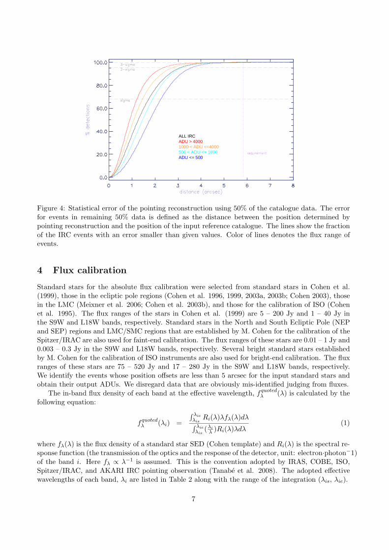
The relations between pipeline output ADUs of events and calculated in-band fluxes of the stan-dard stars are shown in Figures 5 and 6 for the S9W and L18W bands. The relations are nearly linearbut we can see systematic difference from the linear relation (bottom right panels in the figures) whichsuggest that the flux conversion should be made with non-linear functions.

We assume a conversion function as a linear function in log-log scale;

ln(Flux) =∑

i

ai(ln(ADU))i (2)

i.e

Flux = exp

(2∑

i=0

ai(ln(ADU))i

)(3)

where Flux denotes flux in Jy unit and ADU denotes output digital counts from the pipeline. Thecoefficients of the function were derived from least square fitting between pipeline output ADUs andcalculated in-band fluxes of the standard stars. Derived coefficients for S9W and L18W are shown inTable 3.

Table 3: Coefficients of the conversion function for S9W and L18W

band a2 a1 a0

S9W 0.00850918 0.806013 -7.66656L18W 0.00717589 0.829091 -7.35238

The best-fit functions are shown in Figures 5 and 6. The deviations of the fluxes converted withthe derived conversion functions are shown in the bottom panel of the figures. The deviations seemsflat and the fluxes converted with the derived functions reproduce satisfactorily the in-band fluxes.We adopt these functions as conversion functions for the point sources. But we should note that theconversion functions are applicable for the point sources whose fluxes are up to 500 Jy in the S9Wband and up to 300 Jy in the L18W band because of the limits in the calibration standard.

8

0

100

200

300

400

500

600

0 500000 1e+06 1.5e+06 2e+06 2.5e+06 3e+06 3.5e+06

Cal

cula

ted

In-b

and

Flu

x/Jy

Counts/ADU

0

0.5

1

1.5

2

0.01 0.1 1 10 100 1000

Con

vert

ed F

lux/

Cal

cula

ted

In-b

and

Flu

x

Calculated In-band Flux/Jy

0

0.5

1

1.5

2

0.01 0.1 1 10 100 1000

Con

vert

ed F

lux/

Cal

cula

ted

In-b

and

Flu

x

Calculated In-band Flux/Jy

Figure 5: Top: The pipeline output ADUs of events is plotted as a function of the calculated in-bandfluxes of the standard stars in the S9W band. Derived non-linear conversion function for S9W bandare over plotted. Bottom left: The deviations of the ratio of calibrated fluxes with the non-linearconversion function over model fluxes of the standard stars. Bottom right: The deviations of thesame as left but linear conversion function is assumed.

9

0

50

100

150

200

250

300

350

0 200000 400000 600000 800000 1e+06 1.2e+06 1.4e+06

Cal

cula

ted

In-b

and

Flu

x/Jy

Counts/ADU

0

0.5

1

1.5

2

0.01 0.1 1 10 100 1000

Con

vert

ed F

lux/

Cal

cula

ted

In-b

and

Flu

x

Calculated In-band Flux/Jy

0

0.5

1

1.5

2

0.01 0.1 1 10 100 1000

Con

vert

ed F

lux/

Cal

cula

ted

In-b

and

Flu

x

Calculated In-band Flux/Jy

Figure 6: Top: The pipeline output ADUs of events is plotted as a function of the calculated in-bandfluxes of the standard stars in the L18W band. Derived non-linear conversion function for L18Wband are over plotted. Bottom: The deviations of the ratio of calibrated fluxes with the non-linearconversion function over model fluxes of the standard stars. Bottom right: The deviations of thesame as left but linear conversion function is assumed.

10

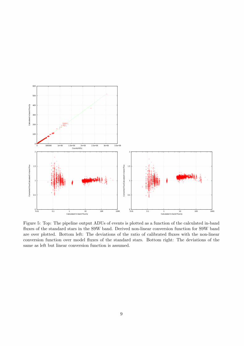
To test the long-term stability of the photo response we investigated five standard stars that havebeen observed more than 30 times during the time of the survey. Figure 7 shows the ratio of thefluxes of individual measurements to the average fluxes of these stars as a function of time. Fromthese data we deduce that the sensitivity is stable at the ∼2% level during the entire period of theobservations.

0.8

0.9

1.0

1.1

05 07 09 11 01 03 05 07 09

Dev

iatio

n

Obs. date (Month in 2006,2007)

HD42540HD45669HD53501HD55865

HD170693

0.8

0.9

1.0

1.1

01 Oct. 02 Oct.

Dev

iatio

n

Figure 7: Ratio of the measured fluxes to the average fluxes as a function of observing time for fivebright (> 1 Jy) standard stars observed at 9µm more than 30 times during the survey. The stars usedand the corresponding 9µm fluxes and number of detections are: HD42540 (plus, 8.33 Jy, 44 times),HD45669 (cross, 9.79 Jy, 43 times), HD53501 (star, 9.30 Jy, 45 times), HD55865 (open box, 16.7 Jy,33 times) and HD170693 (filled box, 9.60 Jy, 76 times), respectively. The closeup shown in the rightbottom panel is to check for the temporal variation on a short timescale.

Laboratory measurements of the filter transmission indicate possible blue leaks between the 3µmand 4µm for the 9µm band and between the 6µm and 7 µm for the 18 µm band. They are 0.01% atmaximum and much smaller than the measurement errors. Thus the presence of the blue leaks is notconfirmed. We calculated the predicted fluxes of the standard stars with and without the blue leakand confirmed that the difference is less than 0.1%. We have verified that the blue leak of the 18µmband is negligible (< 1%) compared to the systematic errors by using asteroid calibrators whose fluxcan be well predicted (Muller & Hasegawa, private communication).

11

5 Catalogue generation

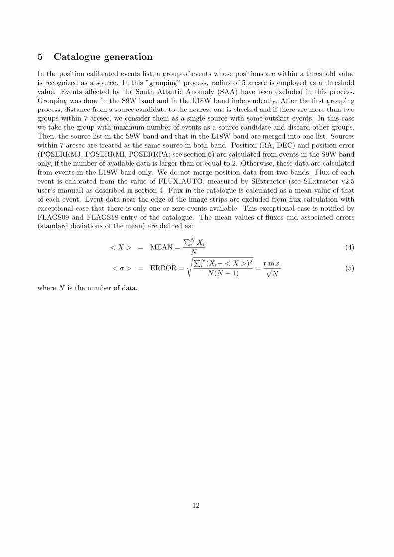
In the position calibrated events list, a group of events whose positions are within a threshold valueis recognized as a source. In this ”grouping” process, radius of 5 arcsec is employed as a thresholdvalue. Events affected by the South Atlantic Anomaly (SAA) have been excluded in this process.Grouping was done in the S9W band and in the L18W band independently. After the first groupingprocess, distance from a source candidate to the nearest one is checked and if there are more than twogroups within 7 arcsec, we consider them as a single source with some outskirt events. In this casewe take the group with maximum number of events as a source candidate and discard other groups.Then, the source list in the S9W band and that in the L18W band are merged into one list. Sourceswithin 7 arcsec are treated as the same source in both band. Position (RA, DEC) and position error(POSERRMJ, POSERRMI, POSERRPA: see section 6) are calculated from events in the S9W bandonly, if the number of available data is larger than or equal to 2. Otherwise, these data are calculatedfrom events in the L18W band only. We do not merge position data from two bands. Flux of eachevent is calibrated from the value of FLUX AUTO, measured by SExtractor (see SExtractor v2.5user’s manual) as described in section 4. Flux in the catalogue is calculated as a mean value of thatof each event. Event data near the edge of the image strips are excluded from flux calculation withexceptional case that there is only one or zero events available. This exceptional case is notified byFLAGS09 and FLAGS18 entry of the catalogue. The mean values of fluxes and associated errors(standard deviations of the mean) are defined as:

< X > = MEAN =∑N

i Xi

N(4)

< σ > = ERROR =

√∑Ni (Xi− < X >)2

N(N − 1)=

r.m.s.√N

(5)

where N is the number of data.

12

6 Catalogue contents and format

The contents of the current version AKARI/IRC PSC are summarized in Table 4. The cataloguewill be distributed in two ways: a FITS file and access via DARTS database query. DARTS interfacewill be provided later. The current version does not include complete information. The contentsand format are carefully defined for permanent use, but we do not rule out the possibility of futureupdates according to the user’s feedback or technical progresses.

Table 4: Contents of the AKARI/IRC Point Source Catalogue

Name Type Format Column Description

OBJID int32 I10 1 – 10 AKARI source ID number.OBJNAME string 15A 11 – 25 AKARI source name. The format is HHMMSSS+/-DDMMSSRA double F10.5 26 – 35 Right Ascension (J2000)[deg]DEC double F10.5 36 – 45 Declination (J2000)[deg]POSERRMJ float F8.2 46 – 53 Major axis of position error ellipse [arcsec]POSERRMI float F8.2 54 – 61 Minor axis of position error ellipse [arcsec]POSERRPA float F8.2 62 – 69 Position angle of Major axis [deg]FLUX09 float E11.3 70 – 80 Flux density in S9W [Jy]FLUX18 float E11.3 81 – 91 Flux density in L18W [Jy]FERR09 float E10.2 92 – 101 Flux error in S9W [Jy]FERR18 float E10.2 102 – 111 Flux error in L18W [Jy]FQUAL09 int16 I2 112 – 113 Flux quality flag for S9WFQUAL18 int16 I2 114 – 115 Flux quality flag for L18WFLAGS09 int16 Z5 116 – 120 Bit flags data quality for S9W. 1: not month confirmed, 2: (not used

in this version), 4: (not used in this version), 8: use edgeFLAGS18 int16 Z5 121 – 125 Bit flags data quality for L18W. 1: not month confirmed, 2: (not used

in this version), 4: (not used in this version), 8: use edgeNSCANC09 int16 I5 126 – 130 Number of scans in which the source is detected for S9WNSCANC18 int16 I5 131 – 135 Number of scans in which the source is detected for L18WNSCANP09 int16 I5 136 – 140 Total number of scans that possibly observed the source for S9WNSCANP18 int16 I5 141 – 145 Total number of scans that possibly observed the source for L18WMCONF09 int16 I3 146 – 148 1 is month confirmed and 0 is not. Inverted value of 1st bit of FLAGS09MCONF18 int16 I3 149 – 151 1 is month confirmed and 0 is not. Inverted value of 1st bit of FLAGS18NDENS09 int16 I4 152 – 155 Number of sources in 45 arcsec radius for S9WNDENS18 int16 I4 156 – 159 Number of sources in 45 arcsec radius for L18WEXTENDED09 int16 I3 160 – 162 Extended source flagEXTENDED18 int16 I3 163 – 165 Extended source flagMEAN AB09 float F8.2 166 – 173 The average of major and minor axes of source extent for S9W [arcsec]MEAN AB18 float F8.2 174 – 181 The average of major and minor axes of source extent for L18W [arcsec]NDATA POS int16 I5 182 – 186 Number of events which are used for positional calculationNDATA09 int16 I5 187 – 191 Total number of events that contribute to the measurements for

FLUX09NDATA18 int16 I5 192 – 196 Total number of events that contribute to the measurements for

FLUX18

13

Description

OBJIDSource ID number.

OBJNAMESource name from its J2000 coordinates, following the IAU Recommendations for Nomen-clature (2006). The format is HHMMSSS±DDMMSS, e.g., 0123456+765432 for a source at(01h23m45.6s, +76d54m32s). The source must be referred to in the literatures by its full name:AKARI-IRC-V1 J0123456+765432, where V1 refers to the version code.

RA, DECJ2000 Right Ascension and Declination of the source position in degree.

POSERRMJ, POSERRMI, POSERRPAOne-sigma error of the source position expressed by an ellipse with Major and Minor axes[arcsec], and Position Angle [deg; East from North]. If only two events are available, POSER-RMJ is calculated from the distance of the two events and POSERRMI is set to the same asPOSERRMJ.

FLUX09, FLUX18Flux density of the source in the two IRC bands in Jansky.

FERR09, FERR18Flux error in the two IRC bands. Errors are defined as equation 5.

FQUAL09, FQUAL18Flux density quality flag in the two IRC bands. 3 when flux is valid and 0 when flux is notavailable.

FLAGS09, FLAGS18Bit flags of data quality:1(LSB): not month confirmed

This means that the period between the first detection and the last detection is shorterthan a month.

2: saturated (not used in this version)4: use SAA (not used in this version)8(MSB): use edge events

If the number of events is too small, we use the event data near the edge of the imagestrip. In this case, this flag warn you of underestimation of the flux.

NSCANC09, NSCANC18Number of scans on which the source is detected. Normally, NSCANC is less or equal toNSCANP. In some exceptional case, resultant position of the source drops out from the imagestripe boundary and NSCANC is larger than NSCANP.

NSCANP09, NSCANP18The number of times the source position has been scanned during the survey.

MCONF09, MCONF181 is month confirmed and 0 is not. Inverted value of LSB of FLAGSxx.

NDENS09, NDENS18The number of sources in 45 arcsec radius.

14

EXTENDED09, EXTENDED18The flag indicates that the source is possibly more extended than the point spread function.This is ”TRUE” when MEAN AB > 15.6 [arcsec]

MEAN AB09, MEAN AB18The average of radius along major and minor axes of images, i.e. (< a > + < b >)/2 where< a > and < b > are the mean semi-major and semi-minor axis lengths of images estimated bySExtractor.

NDATA POSNumber of events used to calculate the mean coordinates. If the source has more than twoavailable S9W events, the position is estimated from S9W events only, else the position isestimated from L18W events, i.e.NDATA POS = NSCANC09 for NSCANC09 ≥ 2NDATA POS = NSCANC18 for NSCANC09 < 2

NDATA09, NDATA18Number of events that contribute to the flux measurements in the two bands. Normally, eventsnear the edge of the image strip are excluded from the measurements. Note that if only 0 or 1event are available, the flux is computed also from edge events.

15

7 Performance

7.1 Number of sources

The AKARI/IRC Point Source Catalogue contains 870,973 sources, out of which 844,649 are detectedin the S9W band and 194,551 in the L18W band. Observations exist in both bands for 168,227sources.As shown in Table 5, by far the largest fraction of sources is detected in the flux range 0.1 to 1 Jy(73% at S9W and 76 % at L18W).

Events affected by the South Atlantic Anomaly (SAA) are excluded from the catalogue.

Table 5: Number(N) of detected sources as a function of flux level

Range Jy N (S9W) N (L18W)0 − 0.1 146,817 1,3170.1 − 1 619,561 148,6751 − 10 71,254 39,321

10 − 100 6,580 4,750100 − 1000 444 478

> 1000 2 10total 844,649 194,551

Table 6: Number of cross matches of the AKARI/IRC PSC with 2MASS sources.

Survey Number of Sources Search radius Matching Sources2MASS 2862152 3′′ 716021

Table 6 provides the results of a cross correlation between the AKARI/IRC PSC and the 2MASSsurvey. For the 2MASS catalogue, the search has been limited to magnitude J = 10.

16

7.2 Extended sources

Figure 8 shows the dependence of MEAN AB on flux. This figure provides the possibility of dis-tinguishing between two populations of sources: extended and point sources. In this version of thecatalogue, extended sources are defined as those with MEAN AB ≥ 15.6 [arcsec], and the associatedEXTENDED flag is set to unity. This flag is based on a fixed threshold value. We note, however,that also bright point source might appear as extended. The histogram in Figure 9 shows clearly thatthe distribution of these parameters is dominated by point sources.

Figure 8: MEAN AB as a function of the S9W (top) and L18W (bottom) flux.

17

Figure 9: Histogram of MEAN AB for S9W (top) and L18W (bottom).

18

7.3 Accuracy of coordinates

For a given source, the distribution of the repeatability errors on coordinates can be described asan error ellipse, whose minor and major axis are defined as the observed minimum and maximumstandard deviation of the distribution, and the position angle is that of the major axis. A test ofthe internal accuracy of AKARI coordinates is given Figure 10, showing the minor axis of the errorellipse as a function of that of the major axis. One can easily appreciate that the errors cluster around0.2′′–0.3′′.

Figure 10: Position repeatability. Sources used in this plot has more than two events. Radius size oferror ellipsoid estimated from the positions of events attributed the same object is plotted as a point.

We have tested the accuracy of coordinates of the AKARI/IRC PSC sources through a cross-match with the the 2MASS survey. Figure 11 show the number AKARI/IRC PSC sources matchingwith the 2MASS J, H and K survey as a function of the seach radius. While too many sources remainunmatched for the case of search radius is 1′′, there is no substantial gain by increasing it above 3′′,a value that is adopted in the following.

Figure 12 shows the histogram of the angular separation between the AKARI/IRC PSC coor-dinates and the 2MASS reference coordinates for cross matched sources. According to these data,nearly 95% of the sources have an angular separation ≤ 2′′, while about 73 % have a separation ≤ 1′′.The mean angular separation between AKARI and 2MASS coordinates of the same sources is 0.765± 0.574 arcsec. Larger internal errors are of course expected for fainter sources, as shown in Figure13.

19

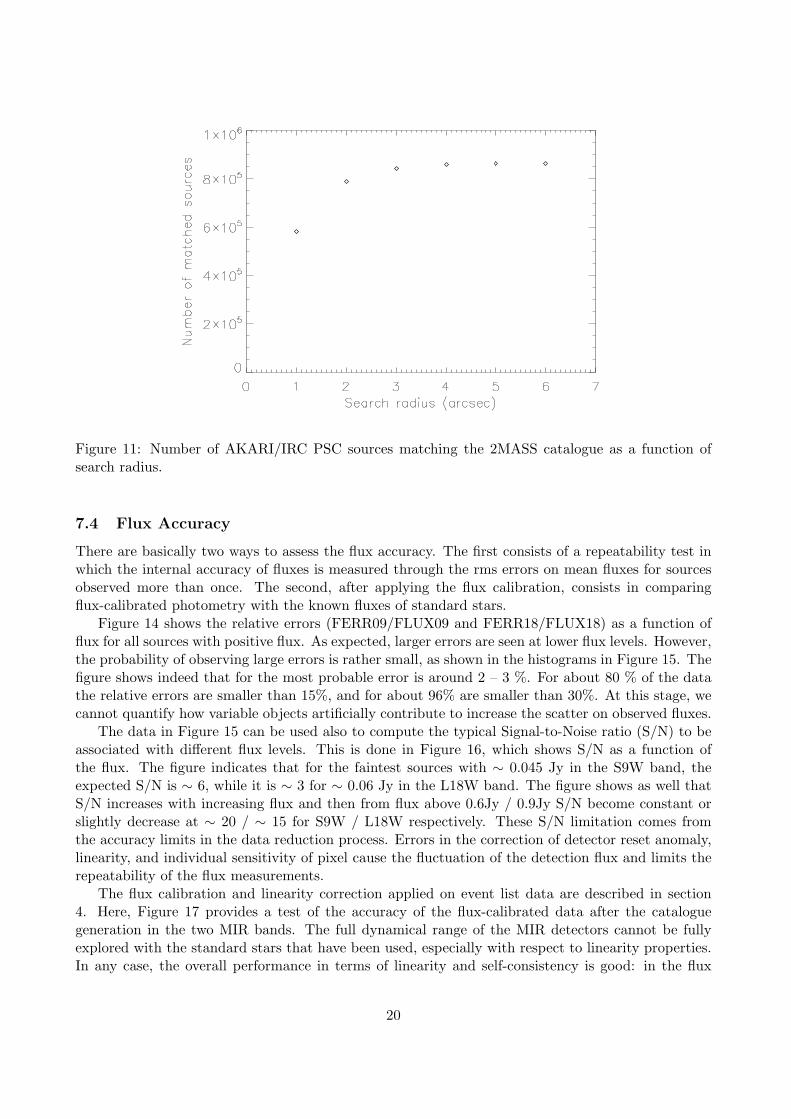
Figure 11: Number of AKARI/IRC PSC sources matching the 2MASS catalogue as a function ofsearch radius.

7.4 Flux Accuracy

There are basically two ways to assess the flux accuracy. The first consists of a repeatability test inwhich the internal accuracy of fluxes is measured through the rms errors on mean fluxes for sourcesobserved more than once. The second, after applying the flux calibration, consists in comparingflux-calibrated photometry with the known fluxes of standard stars.

Figure 14 shows the relative errors (FERR09/FLUX09 and FERR18/FLUX18) as a function offlux for all sources with positive flux. As expected, larger errors are seen at lower flux levels. However,the probability of observing large errors is rather small, as shown in the histograms in Figure 15. Thefigure shows indeed that for the most probable error is around 2 – 3 %. For about 80 % of the datathe relative errors are smaller than 15%, and for about 96% are smaller than 30%. At this stage, wecannot quantify how variable objects artificially contribute to increase the scatter on observed fluxes.

The data in Figure 15 can be used also to compute the typical Signal-to-Noise ratio (S/N) to beassociated with different flux levels. This is done in Figure 16, which shows S/N as a function ofthe flux. The figure indicates that for the faintest sources with ∼ 0.045 Jy in the S9W band, theexpected S/N is ∼ 6, while it is ∼ 3 for ∼ 0.06 Jy in the L18W band. The figure shows as well thatS/N increases with increasing flux and then from flux above 0.6Jy / 0.9Jy S/N become constant orslightly decrease at ∼ 20 / ∼ 15 for S9W / L18W respectively. These S/N limitation comes fromthe accuracy limits in the data reduction process. Errors in the correction of detector reset anomaly,linearity, and individual sensitivity of pixel cause the fluctuation of the detection flux and limits therepeatability of the flux measurements.

The flux calibration and linearity correction applied on event list data are described in section4. Here, Figure 17 provides a test of the accuracy of the flux-calibrated data after the cataloguegeneration in the two MIR bands. The full dynamical range of the MIR detectors cannot be fullyexplored with the standard stars that have been used, especially with respect to linearity properties.In any case, the overall performance in terms of linearity and self-consistency is good: in the flux

20

Figure 12: Histogram of the angular separation between AKARI PSC coordinates and the 2MASScoordinates for the common sources.

21

Figure 13: Angular separation between AKARI PSC coordinates and the 2MASS coordinates as afunction of flux.

22

Figure 14: Internal relative errors on the S9W and L18W fluxes as a function of flux.

23

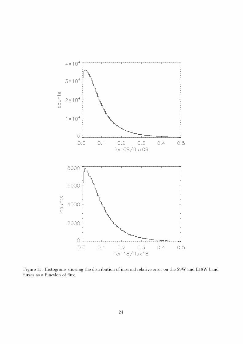
Figure 15: Histograms showing the distribution of internal relative error on the S9W and L18W bandfluxes as a function of flux.

24

Figure 16: Signal to Noise ratio as a function of the S9W and L18W flux.

25

range explored we find: FAKARIν /FStandard

ν = 0.970 ± 0.070(rms) at S9W from 412 measurements,and FAKARI

ν /FStandardν = 1.001 ± 0.045(rms) at L18W from 406 measurements.

26

Figure 17: Flux ratio of AKARI/MODEL in the S9W and L18W bands. MODEL flux is calculatedin-band flux of standard stars and AKARI flux is FLUX09 or FLUX18 in the catalogue. Note thatFLUX09 and FLUX18 is the mean value of events fluxes, whereas Figure 5 and 6 use the fluxes ofevents.

27

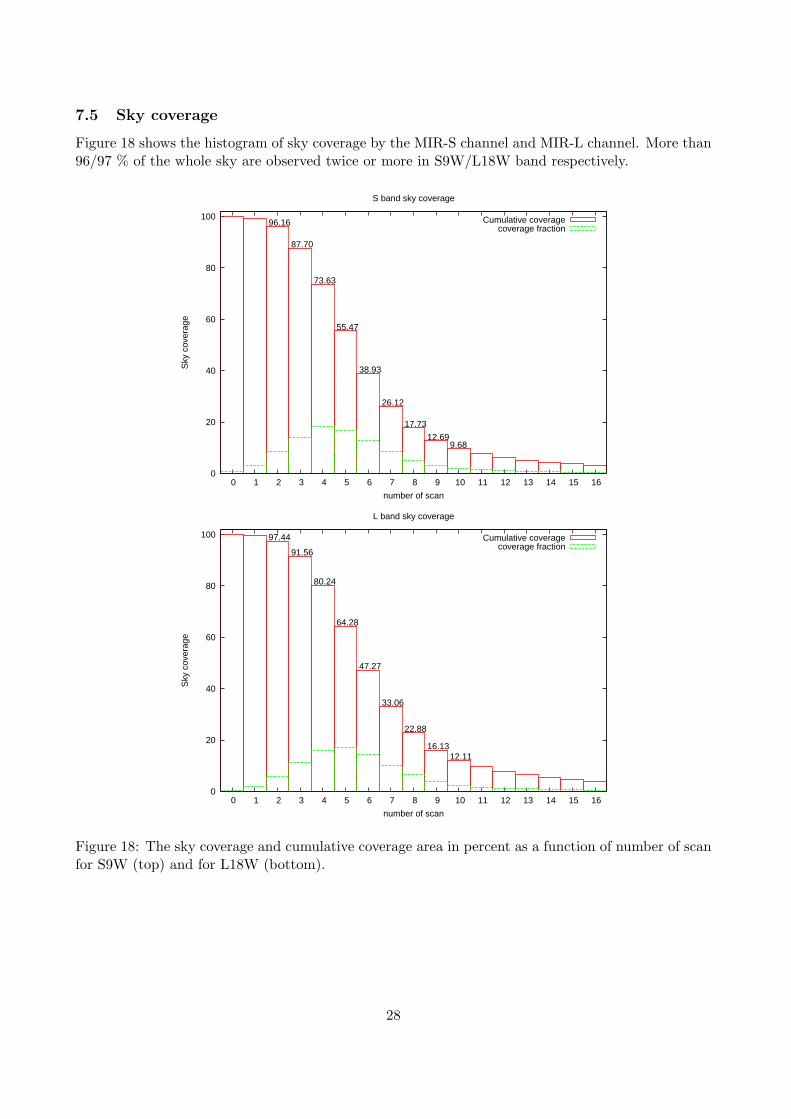
7.5 Sky coverage

Figure 18 shows the histogram of sky coverage by the MIR-S channel and MIR-L channel. More than96/97 % of the whole sky are observed twice or more in S9W/L18W band respectively.

0

20

40

60

80

100

0 1 2 3 4 5 6 7 8 9 10 11 12 13 14 15 16

Sky

cov

erag

e

number of scan

S band sky coverage

96.16

87.70

73.63

55.47

38.93

26.12

17.73

12.699.68

Cumulative coveragecoverage fraction

0

20

40

60

80

100

0 1 2 3 4 5 6 7 8 9 10 11 12 13 14 15 16

Sky

cov

erag

e

number of scan

L band sky coverage

97.44

91.56

80.24

64.28

47.27

33.06

22.88

16.1312.11

Cumulative coveragecoverage fraction

Figure 18: The sky coverage and cumulative coverage area in percent as a function of number of scanfor S9W (top) and for L18W (bottom).

28

7.6 Completeness

The completeness of a survey above a given flux level, is usually defined as the fraction of truesources that can be detected above that level. It is difficult to apply this concept to the AKARIsurvey because one should dispose of a statistically significant sample of true sources with knownIRC fluxes. The standard stars used for the AKARI/IRC PSC calibration might not represent astatistically significant sample, also in view of the rather poor coverage at low flux levels.

To assess the completeness of the AKARI-MIR survey we have thus taken a different approach,based on the distribution of sources according to their flux. Figure 19 shows the histogram of AKARIMIR sources in the S9W and L18W bands with a similar histogram for the IRAS PSC sources. Thishistograms show an interesting feature: source counts decline exponentially after a peak value isreached around 0.1 Jy (S9W) and 0.2 Jy (L18W). This is better seen in Figure 20, where the followingregressions lines have been over plotted to the data:

log(N) = 2.89 − 1.97 log(Flux09)

log(N) = 2.59 − 1.77 log(Flux18)

One can thus make the reasonable assumption that the exponential decay is an intrinsic property ofsource counts at the relevant wavelengths and, on this basis, one can define completeness as the ratioof the number of sources actually observed by the number of sources predicted by the above equations.The results of completeness are shown in Figure 21. From this figure we deduce the completenessrations reported in Table 7. †

Table 7: Completeness and Signal-to-Noise ratio

S9WCompleteness 5% 50% 80% 100%Flux[Jy] 0.06 0.09 0.12 0.20S/N 6.0 7.9 8.5 11.3

L18WCompleteness 5% 50% 80% 100%Flux[Jy] 0.10 0.17 0.22 0.30S/N 5.0 6.8 8.0 9.0

To evaluate the detection limit of the survey, we can make use of the AKARI/IRC PSC Signal-to-Noise characteristics shown in Figure 16. From this figure one can deduce that, for S/N ∼ 5, thedetection limit is about 0.05 and 0.09 Jy in the S9W and L18W bands, respectively.

A summary of the completeness of the survey at various flux levels, together with the correspond-ing values of the Signal-to-Noise ratio are given in the Table 7. These results are in fairly goodagreement with Ishihara et al. (2006, 2008).

†Values are slightly different from Ishihara 2010 which based on the previous version of the catalogue.

29

Figure 19: The distribution of sources as a function of the S9W and L18W flux for AKARI/IRC PSCis compared with that from the IRAS survey at 12 µm and 25 µm in log-log scale.

30

Figure 20: The distribution of sources as a function of the S9W and L18W flux for AKARI/IRCPSC. The over plotted dash-dotted line is a fit to the source counts for fluxes above the peak of thedistribution. Plot in black shows the distribution of all sources in the catalogue, and plots are madealso for galactic latitudes, |b| < 2.2◦ (green), 2.2◦ < |b| < 8.3◦ (blue), and |b| > 8.3◦ (red), separately.

31

Figure 21: Completeness ratio of the AKARI/IRC survey in the S9W and L18W bands. Plot inblack shows the ratio for whole sky, and plots are made also for galactic latitudes, |b| < 2.2◦ (green),2.2◦ < |b| < 8.3◦ (blue), and |b| > 8.3◦ (red), separately.

32

REFERENCES

Bertin, E., and Arnouts, S., 1996 A&AS 317, 393Bertin, E. SExtractor v 2.5 User’s manualBeichman, C. A., Neugebauer, G., Habing, H. J., Clegg, P. E., & Chester, T. J. 1988, Infraredastronomical satellite (IRAS) catalogs and atlases, Explanatory supplem ent, 1Cohen, M., et al. 1992 AJ, 104, 1650Cohen, M., et al. 1995 AJ, 110, 275Cohen, M., et al. 1996 AJ, 112, 2274Cohen, M., et al. 1999 AJ 117, 1864Cohen, M., et al. 2003a AJ, 125, 2645Cohen, M., et al. 2003b AJ, 126, 1090Cohen, M. 2003 in Proc. The Calibration Legacy to the ISO Mission, ESA SP-481, 135IAU Recommendations for Nomenclaturer, Version 2006 November 28, http://cdsweb.u-strasbg.fr/iau-spec.htmlIshihara, D., et al., 2006 PASP 118, 324Ishihara, D., et al., 2008 SPIE 7010, 70100B-1Ishihara, D., et al., 2010 A&Ap acceptedKawada, M., et al., 2007 PASJ 59, S389Lorente, R., et al. AKARI IRC Data User Manual version 1.4 2008Murakami, H., et al., 2007 PASJ 59, S369Onaka, T., et al., 2007 PASJ 59, S401Tanabe, T., et al., 2008 PASJ 60, S375

33

Changes from beta version

• In the milli-seconds confirmation process, we ruled out fake detections more strictly than beta1 version. As a result, number of catalogued source is reduced.

• Number of scan is counted for each source.

• Number of scan map is generated and we can estimate have sky coverage.

• Format of the catalogue is changed.OBJECTID → OBJIDNAME → OBJNAMEFVARxx → removed

34