IT 14 047

Examensarbete 15 hpAugusti 2014

Airspace Sectorisation Using Constraint-Based Local Search

Patrik Ehrencrona Kjellin

Institutionen för informationsteknologiDepartment of Information Technology

Teknisk- naturvetenskaplig fakultet UTH-enheten Besöksadress: Ångströmlaboratoriet Lägerhyddsvägen 1 Hus 4, Plan 0 Postadress: Box 536 751 21 Uppsala Telefon: 018 – 471 30 03 Telefax: 018 – 471 30 00 Hemsida: http://www.teknat.uu.se/student

Abstract

Airspace Sectorisation Using Constraint-Based LocalSearch

Patrik Ehrencrona Kjellin

Airspace sectorisation is the optimisation problem of dividing a given airspace intosectors in a way that promotes efficient air traffic management by some quantifiablemeasure. In this thesis, we apply constraint-based local search on real world airspacedata collected from airports in Europe, given a selection of relevant constraints.

Tryckt av: Reprocentralen ITCIT 14 047Examinator: Olle GällmoÄmnesgranskare: Jean-Noël MonetteHandledare: Pierre Flener

Acknowledgements

I would like to express my gratitude and appreciation to my supervisor PierreFlener, for providing me with such an interesting problem, and for his continuedencouragement and support. Thank you Jean-Noel Monette, for offering invaluableinsight and advice on the programming aspect of this project. Thanks Peter Jagare,for taking the time to meet with me and helping me a great deal with ASTAACand discussing the problem in general.

Contents

1 Introduction 11.1 Airspace Sectorisation . . . . . . . . . . . . . . . . . . . . . . . . . . . . 11.2 Combinatorial Optimisation and Objective . . . . . . . . . . . . . . . . . 11.3 Objective . . . . . . . . . . . . . . . . . . . . . . . . . . . . . . . . . . . 11.4 Choices . . . . . . . . . . . . . . . . . . . . . . . . . . . . . . . . . . . . 1

2 Constraint Programming 22.1 Constraint Problems . . . . . . . . . . . . . . . . . . . . . . . . . . . . . 22.2 Local Search . . . . . . . . . . . . . . . . . . . . . . . . . . . . . . . . . . 32.3 Metaheuristics . . . . . . . . . . . . . . . . . . . . . . . . . . . . . . . . . 4

2.3.1 Tabu Search . . . . . . . . . . . . . . . . . . . . . . . . . . . . . . 52.3.2 Simulated Annealing . . . . . . . . . . . . . . . . . . . . . . . . . 52.3.3 Other Metaheuristics . . . . . . . . . . . . . . . . . . . . . . . . . 6

3 Tools 63.1 OscaR.cbls . . . . . . . . . . . . . . . . . . . . . . . . . . . . . . . . . . . 63.2 ASTAAC . . . . . . . . . . . . . . . . . . . . . . . . . . . . . . . . . . . 6

4 Model 64.1 Data and Pre-Processing . . . . . . . . . . . . . . . . . . . . . . . . . . . 64.2 Sectorisation Constraints . . . . . . . . . . . . . . . . . . . . . . . . . . . 7

4.2.1 Background Geometry . . . . . . . . . . . . . . . . . . . . . . . . 94.2.2 Connectedness . . . . . . . . . . . . . . . . . . . . . . . . . . . . . 104.2.3 Balanced Workload . . . . . . . . . . . . . . . . . . . . . . . . . . 134.2.4 Minimum Dwell Time: Minimum Stretch Sum . . . . . . . . . . . 154.2.5 Minimum Distance: No Border Vertices in Stretches . . . . . . . . 164.2.6 Compactness . . . . . . . . . . . . . . . . . . . . . . . . . . . . . 17

4.3 Constraint Implementations in OscaR.cbls . . . . . . . . . . . . . . . . . 19

5 Search 245.1 Algorithm . . . . . . . . . . . . . . . . . . . . . . . . . . . . . . . . . . . 245.2 Parameters . . . . . . . . . . . . . . . . . . . . . . . . . . . . . . . . . . 26

6 Post-Processing 27

7 Experiments 277.1 Results . . . . . . . . . . . . . . . . . . . . . . . . . . . . . . . . . . . . . 277.2 Improving Sector Shapes . . . . . . . . . . . . . . . . . . . . . . . . . . . 30

8 Discussion 368.1 Conclusion . . . . . . . . . . . . . . . . . . . . . . . . . . . . . . . . . . . 368.2 Future Work . . . . . . . . . . . . . . . . . . . . . . . . . . . . . . . . . . 37

1 Introduction

1.1 Airspace Sectorisation

An airspace sectorisation is the partitioning of airspace into a given number of controlsectors subject to a variety of geometric and workload constraints [4, 3]. In air trafficmanagement (ATM), pairs of controllers are assigned the task of handling all traffic insuch a sector. Historically and presently, airspace has been divided primarily accordingto national borders with little concern for efficient ATM operation. In the ongoing workof creating better sectorisations more suited for efficient operation, a number of differentcriteria have been proposed, many of which are listed in Section 4.2.

1.2 Combinatorial Optimisation and Objective

Optimisation problems in general are ubiquitous and have been subject to much research.In many cases for hard combinatorial problems, finding optimal solutions can be so costlythat it is better to use approximation algorithms for finding near optimal solutions.Stochastic local search (SLS, see [5] for instance) is one example of such an algorithmdesign technique which has been successfully applied on a wide range of problems.

1.3 Objective

In this thesis, we implement a constraint-based local search (CBLS, see [16] and [5])approach to the problem of airspace sectorisation. The differences with the prior thesis[7], which has almost the same objective, are that here we are going to use local search,whereas in [7] systematic search was used, and that [7] is a master thesis whereas thisis a bachelor thesis. The differences with the paper [8], which has the same technicalobjective, are that we benefit from the new insights of [3] and that our non-technicalobjective is to demonstrate how far a novice in ATM and CBLS can go in only 10 weeks,when using the right tools.

1.4 Choices

All the constraint descriptions, as well as the background geometry detailed in Section 4.2are taken from [3] with full permission granted from the authors, the first of whichbeing the supervisor of this thesis. These descriptions are the basis for all constraintsimplemented for the purpose of this thesis.

Rather than implementing all search and modelling components from scratch, we usethe pre-existing solver OscaR.cbls with a dedicated framework for the implementation ofconstraints and invariants.

Code for the pre-processing of the data to be used for experiments is taken directlyfrom [8], with permission granted from its authors.

In order to make this thesis self-contained, the initial Section 2 contains a brief over-view of constraint programming (CP) in general and CBLS in particular. In Section 3, wepresent the tools utilised for the making and evaluation of our sectorisation algorithm. Wethen move on to describing the relevant data and the structure of our model in Section 4,and present the search algorithm and post-processing in Sections 5 and 6. In Section 7,

1

we present the results of our work. In Section 8 we give our conclusions and elaborate onthe tasks, beyond the scope of this thesis, that lie ahead in airspace sectorisation.

2 Constraint Programming

CP is a programming paradigm wherein a problem is defined as a set of decision variableswith relations imposed on them by declarative constraints. [1, 3] In essence, constraintsdefine the properties of the sought solution and guide the search toward an optimisedstate. There are clear benefits to using declarative constraints kept separate from thesearch component of the solver. Namely, constraints are handled in a plug-and-playmanner, which gives rise to high code reusability and modularity.

2.1 Constraint Problems

A constraint satisfaction problem [1] (CSP) in its most basic form consists of:

• A set of decision variables {x1, . . . , xn}.

• For each decision variable xi, a finite domain dom(xi) of its possible value assign-ments. The domain of a variable need not necessarily be comprised of integers.

• A set of constraints {c1, . . . , cm} imposed on decision variables.

A solution is an assignment of the decision variables to values in their domains such thatall constraints are satisfied in systematic search, or violated to a sufficiently low degreein local search. [3, 5] In CBLS, the sum of the violations of all constraints constitutethe objective function, which is to be minimised. Within the context of local search, acandidate solution is any assignment of decision variables to values in their domains.

Besides the basic binary constraints (=, <, >, ≤, ≥, 6=), many advanced globalconstraints have been invented for the modelling of all kinds of complex problems. Forexample, the Linear({x1, x2, ..., x3}, RelOp, c) constraint ensures that the sum of {x1,x2, ..., x3} is in relation RelOp ∈ {=,<, >,≤,≥, 6=} with c. Another example of a globalconstraint is AllDifferent({x1, x2, ..., xn}), which penalises non-distinct values inthe n decision variables. The violations of AllDifferent as well as Linear can, forexample, be measured by the number of moves required to fully satisfy them. Many otherglobal constraints can be found in [2].

Constraint programming consists of two components, modelling and search. [3, 1]During the modelling stage, choices have to be made on how the problem should berepresented in terms of decision variables, variable domains, and constraints. Creating asuitable model is imperative for the performance of CP and can often be quite tricky. Toillustrate the importance of good modelling it may be helpful to start off by presentinga naıve CP approach to solving the NQueens problem, which will be used as a runningexample throughout this section.

2

The NQueens problem consists of placing N chess queens on an N ×N chess boardin such a way that none of them threaten each other. That is, none of the queensmay share the same row, column, or diagonal on the board.

Example 2.1 Let the board be represented as an N×N Boolean matrix B[1..N ][1..N ] ofN2 decision variables, where for each position on the board B[i][j] = 1 means the squareBi,j is occupied by a queen, whereas B[i][j] = 0 represents an empty square.

Now it is time to apply some constraints on the decision variables. The Linearconstraint, for example, can be applied on each row, column, and diagonal with parametersRelOp = ≤ and c = 1.

Example 2.2 Another way to model the same problem is to represent the row position ofeach queen as an array Q[1..N ] of only N decision variables, each with domains {1, ..., N}.Here, the index represents the column position of the queen, and so the queens are keptseparate in the columns by the formulation of the problem. Additionally, the requiredAllDifferent constraint imposed on the columns can be handled implicitly (i.e., theyare satisfied in the initial assignment and may never be broken), by only applying moveswhere the values of pairs of queens are swapped. Not only does this result in a significantlysmaller amount of decision variables, the problem also requires fewer constraints. TwoAllDifferent constraints applied on the diagonals are now sufficient for solving theproblem.

2.2 Local Search

The standard approach to searching in constraint programming, systematic search [3, 1],involves pruning the domains of decision variables until either a solution is found, or isdecidedly confirmed not to exist. Under systematic search, the entirety of the searchspace (that is, the set of all variable assignments) is explored. Local search [3, 5], on theother hand, trades the completeness property of systematic search in favour of speed andefficacy. In local search, an initial location of the search space is selected with possiblyrandom assignments to each decision variable. The search then proceeds by iterativelymoving to neighbouring solutions that differ from the current solution only in one or afew of its decision variables.

Navigating through the search space by some sort of inference process can be donein several manners. A simplistic search procedure might select the most improving movein each iteration. More often than not, in real applications, other techniques must beapplied in order for the search to be able to escape local optima in the underlying objectivefunction, or in order to narrow down the search space to a manageable size. [5]

Example 2.3

Continuing with the NQueens model of Example 2.2, one might carry out a search by, ineach iteration, identifying the two most violating queens and row-wise swapping them.For a problem of size N = 4, and an initial assignment {x1 = 1, x2 = 2, x3 = 3, x4 = 4},each queen contributes to the violation of a diagonal AllDifferent constraint. Recall

3

that the violation of this constraint is equal to the number of moves necessary to resolvethe conflict, and so the constraint violation becomes 3. The sum of the violations of bothconstraints in the system constitutes the objective function, which in this case wouldobtain a value of 3.

4 0Z0L3 Z0L02 0L0Z1 L0Z0

x1 x2 x3 x4

4 0Z0L3 Z0L02 QZ0Z1 ZQZ0

x1 x2 x3 x4

4 0L0Z3 Z0L02 QZ0Z1 Z0ZQ

x1 x2 x3 x4

4 0L0Z3 Z0ZQ2 QZ0Z1 Z0L0

x1 x2 x3 x4

Considering any pair of queens, after having exchanged values, would cause a decrease inthe objective function, any pair is eligible for a swap move. In the case when several movesare as good, one is typically randomly selected. If we proceed with a x1 :=: x2 move, thetwo constraints obtain a violation of 1, causing the objective function to decrease by 1.Similarly, x2 :=: x4 and x3 :=: x4 are subsequently selected before the problem is solved.The figure above, from left to right, shows the state of the board after each consecutivemove, with the leftmost board being the initial assignment.

When comparing a set of possible moves, rather than actually performing each moveand subsequently reversing it in order to measure the change in the objective function, itis often preferable to use a delta function that efficiently measures the impact of a givenmove. OscaR.cbls does not support delta functions, hence we do not discuss them in thisthesis, but we refer to [16] for details.

2.3 Metaheuristics

A fundamental problem associated with local search is its tendency to get stuck withinlocal minima of the underlying objective function. Local search in its simplest form,called iterative improvement, starts from some possibly randomly selected point in thesearch space and merely moves to a neighbouring candidate solution that improves theobjective function. In this type of primitive search, moving away from local optima isnot possible as any such move will be promptly undone in subsequent iterations. In orderto address this problem, a variety of sophisticated mechanisms exist for escaping localminima. In many cases, using a hybrid of several such heuristics can additionally improvethe performance of the search. [5]

4

2.3.1 Tabu Search

1

2

3

4

5

Tabu search (TS, see [5]) is a common technique that hasbeen successfully applied on numerous optimisation prob-lems. It extends the iterative improvement strategy by intro-ducing a list of forbidden moves derived from recent searchhistory.

A generic approach to building the tabu list is to markany decision variable involved in a move as prohibited forthe next n iterations, where the value of n has to be tunedexperimentally. In order to illustrate the benefits of prohib-iting certain moves, consider a search space with 5 differentstates, as depicted to the left. Let the objective function

(which is to be minimised) for each state 1..5 evaluate according to: Objective(1) := 3,Objective(2) := 1, Objective(3) := 4, Objective(4) := 0, and Objective(5) := 2. If thesearch is initialised at state 1 in the search space, an iterative improvement strategy(selecting either the most improving or least worsening move) will move to state 2 as itis the most improving among the immediate neighbours. In the next step, however, thesearch will be inclined to move back to state 1, as that is the least worsening move.

It is clear that this approach is not going to succeed in finding an optimal solution.Now let us imagine that upon moving to state 2 in the first iteration, we forbid the searchfrom moving to state 1 in the subsequent n = 1 iterations. The search is forced to moveto the worsening state 3, upon which the globally optimal solution in state 4 is withinreach.

The value of n, or the length of the tabu has a large impact on the performance ofTS, as the goal is to escape local minima without moving to a more worsening candidatesolution than absolutely necessary. In some instances, it is beneficial to dynamicallyadjust the tabu length during the search in such a way that it increases as the searchapproaches a local minimum, and decreases whenever the search enters an escape phase.

TS can also be enriched with various aspiration criteria, which allow certain solu-tions of some desired quality (or alternatively, for diversification purposes) to bypass therestriction.

2.3.2 Simulated Annealing

The idea behind simulated annealing (SA, see [5]) is to occasionally accept worseningmoves, while gradually decreasing their frequency as the search progresses. The accept-ance function for SA determines the probability for accepting a worsening move:

f(∆) =1

1 + e∆T

where ∆ is the change in the objective function upon the move. Because ∆ and T arepositive (since the move is worsening, which is to say the objective function is increasing),the probability for accepting the worsening move is somewhere between 0 and 1

2. The

temperature variable T is systematically decreased in each iteration according to somecooling schedule and the annealing parameter k. For example, a schedule resulting in a

5

fairly rapid decrease in T is Tn =Tn−1k

with the initial temperature T0 being set to some

appropriate constant [5, 6].

2.3.3 Other Metaheuristics

Detailed descriptions of a wide range of sophisticated methods for escaping local minimain local search can be found in [5].

3 Tools

3.1 OscaR.cbls

OscaR.cbls [12] (Scala in OR (Operations Research)), formerly Asteroid, is an open-sourcesolver built on top of Scala. It allows us to create complex models and provides a largeset of tools for the programming of efficient search techniques. Apart from a fairly size-able collection of standard invariants and constraints, OscaR.cbls offers a framework fordeclaring custom, incrementally maintained invariants and constraints. For an in-depthview of the internals of OscaR.cbls, we refer to the OscaR.cbls reference document [9].

3.2 ASTAAC

ASTAAC (Arithmetic Simulation Tool for ATFCM (Air Traffic Flow and Capacity Man-agement) and Advanced Concepts) is a software provided by EUROCONTROL thatcontains real flight data collected from all over Europe and is able to calculate the celland trajectory values for a given sectorisation scenario. For our own experiments, AS-TAAC allowed us to easily generate an airspace divided into a mesh of cells coupled withreal flight data. Furthermore, ASTAAC enabled us to analyse and visualise the resultsof our sectorisation. In order to interface the sectorisation algorithm with ASTAAC, aswell as pre-process data, this work relies completely on the prior work by Peter Jagarein [8].

ASTAAC also ships with a built-in sectorisation algorithm, which uses greedy pro-gramming and shall be used as a benchmark for comparisons with our sectorisations interms of solution quality, performance, etc.

4 Model

4.1 Data and Pre-Processing

Airspace sectorisation can be approached either as a graph colouring or as a set coveringproblem [3]; the constraints described in Section 4.2 were intended for the implementationof the former.

In the graph colouring approach, the background geometry is represented as an un-directed graph G = 〈V,E ⊆ V × V 〉. For each of the n vertices v ∈ V representing acell (or region, here used interchangeably) of the geometry, a decision variable Colour(v)keeps track of its sector i ∈ {1, 2, . . . , k}, where k is the desired number of sectors. The

6

edges E connect the adjacent cells of the geometry. The cells can be in the shape of anytype of polyhedron with flat sides.

ASTAAC conveniently outputs an air control centre (ACC) airspace in the form of amesh of cells, each with an associated workload (see below). In the pre-processing step,cells are then greedily divided into an initial solution of k connected components, whileattempting to maintain reasonably balanced and somewhat compact sectors. ASTAACand the pre-processing algorithm of [8] also provide the option of clustering multiple cellsinto a larger air functional block (AFB), which is guaranteed not to violate the minimumdistance constraint.

The trajectories of aircraft are represented as sequences of cells along with timestampsat each cell entry and exit, and will be used in order to define the minimum dwell time,trajectory-based convexity, and minimum distance constraints.

Because there is usually a lot of overlap in the trajectories, the data is somewhatsimplified by ASTAAC in the form of combining several trajectories into flows. We didhowever refrain from using the flows, as doing so would make it difficult to maintainaccurate violations in certain constraints on the trajectories.

The workload of a given sector (see [3, 4]) is a measure of the amount of work requiredfrom its controllers and can be further categorised as:

1. Monitoring workload, which is the work associated with keeping track of aircrafttrajectories within a sector.

2. Conflict workload from managing conflict avoidance and resolution between flights.

3. Coordination workload, which occurs whenever aircraft traverse between adjacentsectors.

The monitoring and conflict workloads are additive in nature and for that reason only theyare included in the workload values constructed during pre-processing. We use a functionC that takes a set of cells and returns the combined workload for that set considered asa sector. C sums up the workloads of the vertices in a region set R constituting a sector,that is:

C(R) =∑v∈R

Workload(v)

In ASTAAC, some parameters are available for defining the characteristics of the data.For the purpose of testing our sectorisation, we used the default settings unless otherwisespecified, which divides the airspace into hexagonal cells of dimension 5 NM × 5 NM(nautical miles) and a height of 1000 feet.

During search, a large portion of the cells can be mostly ignored as a result of havingan associated workload of zero (we will refer to these as empty cells). These cells neednot be considered for moves as they do not affect the workload or trajectory constraints.They cannot however be completely excluded, as in order to enforce connectivity in thesectors, it is necessary to look at cells that are not part of any trajectory as well.

4.2 Sectorisation Constraints

Several constraints have been proposed in previous work, and details for the implement-ations of constraints were provided for the writing of this thesis in [3]. For simplicity,

7

we will categorise constraints as either hard or soft. Hard constraints must be satisfiedwhereas soft constraints may be violated to some degree in a solution. Some constraintsmay be handled implicitly. Such constraits are satisfied in the initial solution and remainso throughout the search by only allowing non-violating moves (i.e., the way our differentrow constraints were handled in the NQueens problem). Here are the constraints in brief:

Objective Representationc0 Balanced workload Build

sectors in such a way thatthe workload is evenly dis-tributed among the airtraffic controllers.

We impose a soft, explicit constraint Balanced onall the decision variables. Using the workload func-tion C(R), we keep track of the total workload of eachsector of the current solution. We associate a viola-tion with any cell belonging to a sector that deviatesfrom the average workload across all sectors to a cer-tain extent. In order to search for a solution, we onlyneed to consider those cells v where Workload(v) > 0.

c1 Connectedness Make surethat each sector consists ofa single connected compon-ent.

This constraint is hard, and must be satisfied in asolution. We opt to handle it implicitly, by only re-assigning decision variables to sectors such that allsectors retain the connectedness property.

c2 Trajectory-Based Con-vexity Minimise the occur-rence of flights entering asector multiple times.

We impose a soft, explicit constraint Connected oneach of the flight trajectories, represented as arraysof decision variables. The Connected constraintassociates a degree of violation with cells belongingto sector i iff sector i appears as n > 1 connectedcomponents in the trajectory. For this constraint,the neighbourhood is suitably defined as all cells thatlie on the border of a stretch within the trajectories.

c3 Minimum Dwell TimeMinimise the occurrence offlights entering sectors for avery short period of time.

We impose a soft, explicit constraint Stretch-Sum on each of the flight trajectories, represented asarrays of decision variables. The StretchSum con-straint associates a degree of violation with any cellthat is part of a stretch that lingers for less than tseconds in a sector.

c4 Minimum Distance At-tempt to keep flight tra-jectories a certain distancefrom the borders of a sec-tor, in order to avoid con-trollers of multiple sectorshaving to keep track of thesame flights.

We impose a soft, explicit constraint NonBorder oneach of the flight trajectories, represented as arraysof decision variables. A violation is imposed on a cellbelonging to sector i iff an adjacent cell that is notpart of the trajectory is assigned to another sector.This works under the assumption that the cells arelarge enough that a distance of one cell apart fromthe border is sufficient.

c5 Compactness Aim to ob-tain reasonably compactsectors, that are not overlycomplicated for air trafficcontrollers to keep in mind.

We impose a soft, explicit constraint Compact onall the decision variables. The Compact constraintassociates a penalty on any cell belonging to a sectorthat has an above average surface area.

8

Recall that the following subsections, describing the constraints, as well as the geo-metric representation used, are taken with permission from [3], with a correction to theConnected constraint given in Section 4.3.

Below, the current assignment of some decision variable x is denoted by α(x).

4.2.1 Background Geometry

In order to describe the constraints below, a brief overview of the underlying geometryand notation used is required.

When considering constraints on the shape of sectors, we need access to the shape ofits constituent regions. In particular, if we are considering regions that are polytopes,then each region has a number of lower-dimensional facets. In three dimensions, thefacets are two-dimensional surfaces, and in two dimensions, the facets are one-dimensionallines. In algebraic topology [11], there is a very general theory of simplexes, which arerepresentations of geometric objects together with facets, and facets of facets, all theway down until zero-dimensional points are reached. Although we do not need the fullmachinery of algebraic topology, the formalisation given here is inspired by its standardtreatment [11].

Given a graph G = 〈V,E ⊆ V × V 〉, a facet structure for G is a set of facets F and afunction ∂ from vertices V to sets of facets from F . The facet function needs to satisfythe condition that given any two adjacent vertices v and w (that is 〈v, w〉 ∈ E), there isexactly one facet f ∈ F such that f ∈ ∂(v) and f ∈ ∂(w).

A facet f is a border facet if there is exactly one vertex v such that f ∈ ∂(v). A bordervertex is a vertex that has a border facet.

Given a graph G = 〈VG, EG ⊆ VG × VG〉, we denote the set of border vertices of G byBG. The enveloped graph of G, denoted by G⊥, is the graph

〈VG ∪ {⊥} , EG ∪ ({⊥} ×BG) ∪ (BG × {⊥})〉

That is, there is a unique new vertex ⊥ that is connected to all border vertices. Theextended facet function ∂⊥ is defined as

∂⊥(v) =

{∂(v) if v 6= ⊥{⊥} otherwise

Given a graph and a facet structure with facet function ∂, the extended facet functionsatisfies the property that for any v 6= ⊥ and w 6= ⊥ there is exactly one facet f ∈ Fsuch that f ∈ ∂⊥(v) and f ∈ ∂⊥(w).

Sometimes, we need to see a vertex set V as an ordered set:

• Let v ≺ w denote that vertex v is to the left of vertex w in the vertex set V .

• Let v � w denote that vertex v is to the left of vertex w in V , with possibly v = w.

• Let pred(v) denote the predecessor of vertex v in V ; if v is the leftmost vertex inV , then pred(v) = ⊥.

• Similarly, let succ(v) denote the successor of vertex v in V , if any, else ⊥.

9

The vertex set V is seen as a sequence rather than as a set whenever we use the ≺ or �relation to specify the semantics of a constraint.

It will sometimes be useful to have information about the volume of a region and thesurface area of a facet of a region. We assume that we are given two functions:

• Volume: V → N, such that Volume(r) returns the volume of region r.

• Area: V ×F → N, such that Area(r, f) returns the area of facet f or region r, withf ∈ ∂(r). Technically, the region r is a redundant argument, but we keep it forclarity.

We use the terminology of a 3D space. In a 2D space, the facet area would be a sidelength, and the region volume would be a surface area.

For the flights, we assume without loss of generality that time stamps are given asintegers. A flight plan is a sequence of regions, each with an entry time stamp and anexit time stamp, such that the times are increasing between entry and exit time stamps.Formally a flight plan p is a member of (V × N× N)∗ such that if

p = [〈v1, t1, t′1〉 , 〈v2, t2, t′2〉 , . . . , 〈vm, tm, t′m〉]

then for all 1 ≤ i ≤ m we have ti < t′i, and for all 1 ≤ i < m we have t′i = ti+1. Notethat we require a strict inequality between entry and exit timestamps since aircraft havea finite velocity. Let the flight plan of flight f be denoted by Plan(f).

4.2.2 Connectedness

The Connected(G,Colour ,RelOp, N) constraint, with RelOp ∈ {≤, <,=, 6=, >,≥},holds if and only if the number of colours used in the sequence Colour is in relationRelOp with N , and there is a path in the graph G = 〈V,E〉 between any two vertices ofthe same colour that only visits vertices of that colour. Formally:

|{Colour(v) | v ∈ V }| RelOp N ∧∀v, w ∈ V : Colour(v) = Colour(w)⇒ 〈v, w〉 ∈ E∗Colour(v)

(1)

where E∗c denotes the transitive closure of Ec, which is the adjacency relation E projectedonto adjacency for vertices of colour c:

Ec = {〈v, w〉 ∈ E | Colour(v) = c = Colour(w)}

Hence the total number of connected components in the induced graph ColourGraphmust be in relation RelOp with N , and the number of connected components per colourmust be at most 1.

Arbitrary Number of Dimensions. The Connected(G,Colour ,RelOp, N) constraintgeneralises the main aspect of the Connect Points(w, h, d,Colour , N) constraint of [2],which considers RelOp is “=” and considers G to be induced by a w×h×d cuboid dividedinto same-sized regions; further, there is a special colour (value 0) for which there is norestriction on the number of connected components.

The constraint Connected is a hard constraint in prior work on airspace sectorisa-tion using stochastic local search [8], hence no violation and differentiation functions aregiven there.

10

One Dimension. The constraint Connected(G,Colour ,RelOp, N) for a graph G in-duced by a one-dimensional geometry (in which connected components are called stretches)generalises the main aspect of the Multi Global Contiguity(Colour) constraint [2],which itself generalises the Global Contiguity(Colour) constraint of [10]: the lat-ter constrains only one colour (value 1) but the former constrains several colours, andboth lack the decision variable N and hence RelOp; further, both have a special colour(value 0) for which there is no restriction on the number of stretches (there are at mosttwo such stretches when there is only one constrained colour).

The trajectory-based convexity of an airspace sectorisation is achieved by posting forevery flight a Connected(G,Colour ,≤, s) constraint on the sequence Colour of decisionvariables denoting the sequence of colours of its one-dimensional visited region sequenceV , where s is the imposed or maximum number of sectors. The initial domain of eachcolour decision variable Colour(v) is {1, 2, . . . , s}.

Such a trajectory-based convexity constraint is a soft constraint in prior work onairspace sectorisation under stochastic local search [8], but lacks the decision variable Nand hence RelOp; further, the constraint violation is defined differently there (in a mannerthat requires an asymptotically higher runtime to compute than the one we give below),and the variable violation and differentiation functions are not given there (though theyare in the unpublished code underlying the experiments).

Violation Functions. The violation functions described below have no asymptoticallybetter specialisation to the case of G being induced by a one-dimensional space. Hencethey apply to both connectedness in a space of an arbitrary number of dimensions andto contiguity in a one-dimensional space.

If the Connected constraint is considered explicitly, then we proceed as follows. Forrepresenting the induced graph ColourGraph, we show that it suffices to initialise andmaintain the following two data structures, which are internal to the constraint:

• Let NCC (c) denote the number of connected components (CCs) of ColourGraphwhose vertices currently have colour c.

• Let NCC denote the current number of connected components of ColourGraph:

NCC =∑

c∈Colours

NCC (c) (2)

We can now re-formalise the semantics (1): the Connected(G,Colour ,RelOp, N) con-straint is satisfied if and only if

NCC RelOp N ∧ ∀c ∈ Colours : NCC (c) ≤ 1

The violation of a colour decision variable, say Colour(v) for vertex v, is the currentexcess number, if any, of connected components of ColourGraph for the colour of v:

violation(Colour(v)) = NCC (α(Colour(v)))− 1 (3)

This variable violation is zero if v currently has a colour for which there is exactly oneconnected component in ColourGraph, and positive otherwise.

11

The violation of the counter decision variable N is 0 or 1 depending on whether NCCis in relation RelOp with the current value of N :

violation(N) = 1− [NCC RelOp α(N)]

This variable violation is zero if NCC RelOp α(N) currently holds, and one otherwise.The violation of the constraint is the sum of the variable violation of N and the

current excess number, if any, of connected components for all colours:

violation = violation(N) +∑

c∈Colours

max(NCC (c)− 1, 0) (4)

The constraint violation is zero if NCC RelOp α(N) holds and there currently is at mostone connected component in ColourGraph for each colour.

To achieve incrementality, once a move has been picked and made, the internal datastructures and the variable and constraint violations must be updated. The followingupdating code (which contains an error that we will fix in in Section 4.3) for a colour as-signment move Colour(v) := c applies, where the new assignment α′ is the old assignmentα, except that α′(Colour(v)) = c:

1: if ∀w ∈ Adj(v) : α(Colour(w)) 6= c then {v forms a new CC of colour c}2: NCC (c) := NCC (c) + 13: NCC := NCC + 14: violation := violation + 15: end if6: if ∀w ∈ Adj(v) : α(Colour(w)) 6= α(Colour(v)) then {v formed a CC of α(Colour(v))}

7: NCC (α(Colour(v))) := NCC (α(Colour(v)))− 18: NCC := NCC − 19: violation := violation− 1

10: end if11: for all v ∈ V do12: violation(Colour(v)) := α′(NCC (Colour(v)))− 113: end for14: violation(N) := 1− [NCC RelOp α(N)]

Incremental updating for a colour assignment move takes time linear in the degree ofvertex v in G and linear in the number |V | of vertices (and colour decision variables).Code follows similarly for the colour swap and counter assignment moves.

For the remaining constraints, we assume that some relationships among internaldata structures, such as (2), and the violation functions, such as (3) to (4), are defined asinvariants [16], so that the solver automatically updates these quantities incrementally,without the constraint designer having to write explicit code, such as lines 3, 4, 8, 9and 11 to 14.

Hard Constraint. If the Connected constraint is considered implicitly, as in [8], thenit can be satisfied cheaply in the start assignment, by partitioning G into connectedcomponents and setting N according to RelOp, and maintained as satisfied upon everymove, by only considering moves that re-colour a vertex at the border of a connected

12

component to the colour of an adjacent connected component. For instance, if RelOp isequality, then one can partition G into n = max(dom(N)) connected components and setN := n.

4.2.3 Balanced Workload

The Balanced(G,Colour ,Value, µ,∆) constraint holds if and only if the sums of thegiven integer values under Value of the vertices having the same colour under Colour arebalanced, in the sense of having the (possibly unknown, and not necessarily integer) valueµ as average and having discrepancies to µ that do not exceed the (possibly unknown)integer threshold ∆. If ∆ is not given, then it may appear in the objective function,towards being minimised. Formally, the constraint can be decomposed into the followingconjunction:

∀i ∈ Colours : X[i] =∑v∈V

([Colour(v) = i] · Value(v)) ∧ Γ(X,µ,∆)

where constraint Γ is either Spread or Deviation, thereby giving a concrete definitionto the used abstract concept of discrepancy :

• The Spread(X,∆, µ) constraint [13] holds if and only if the n integer variables X[i]have the (possibly unknown, and not necessarily integer) value µ as average andthe sum of the squared differences (n ·X[i]− n · µ)2 does not exceed the (possiblyunknown) integer threshold ∆.

• The Deviation(X,∆, µ) constraint [14] holds if and only if the n integer variablesX[i] have the (possibly unknown, and not necessarily integer) value µ as average andthe sum of the deviations |n ·X[i]− n · µ| does not exceed the (possibly unknown)integer threshold ∆.

The multiplications by n in the definitions of discrepancy lift all reasoning to integerdomains even when µ is not an integer, as

∑ni=1X[i] = n · µ and the X[i] are integer

variables: the integer threshold ∆ has to be calibrated accordingly. One could alsouse the Range(X,RelOp,∆) constraint [2], which holds if and only if max(X) + 1 −min(X) RelOp ∆, but we do not pursue this option further.

In airspace sectorisation, the workload of each sector must be within some givenimbalance factor of the average across all sectors. Hence one would take Value as theWorkload function of Section 4.1. Recall that we only consider additive workloads, suchas monitoring workload and conflict workload, but no non-additive workloads, such ascoordination workload. Note that µ is known when the number n of sectors (and thuscolours) is imposed:

µ =

∑v∈V Workload(v)

n(5)

The workload balancing constraint is a soft constraint in prior work on airspace sec-torisation under stochastic local search [8], but its concept of discrepancy is defined interms of a ratio rather than a difference with the average µ, namely X[i]/µ ≤ 1 + ∆for each i (in the experiments, ∆ = 0.05 was used). This concept of discrepancy is lessrelated to standard concepts in statistics.

13

Violation Functions. We here handle the Balanced constraint for the case Γ =Deviation. Handling the case Γ = Spread can be done using the same ideas. Weassume Colours = {1, 2, . . . , n}.

If the Balanced(G,Colour ,Value, µ,∆) constraint is considered explicitly, then weproceed as follows. For simplicity of notation, we assume ∆ and µ are given, and that µ isan integer. Relaxing these assumptions can be done using the same ideas as below. Themultiplications by the number n of colours in the definition of the underlying Deviationconstraint can then be eliminated, upon dividing ∆ by n2, giving the following simplifiedsemantics of Balanced:

n∑i=1

X[i] = n · µ (6)

andn∑i=1

|X[i]− µ| ≤ ∆ (7)

where∀i ∈ {1, . . . , n} : X[i] =

∑v∈V

([Colour(v) = i] · Value(v)) (8)

Note that (8) impliesn∑i=1

X[i] =∑v∈V

Value(v)

so that, using (6), we must have

µ =

∑v∈V Value(v)

n(9)

similarly to (5). From now on, we assume the given Value and µ satisfy (9), so thatwe need not reason about (6), as it is then surely satisfied, because implied when (8) issatisfied. Formula (8) itself defines the auxiliary decision variables X[i], so it suffices toset it up as a set of invariants [16]. In conclusion, we only need to deal with formula (7).

The violation of a decision variable, say Colour(v) for vertex v, is the same as the viol-ation of the auxiliary decision variable X[α(Colour(v))], which is functionally dependenton Colour(v) under (8). This violation is the current deviation from µ of the value sumfor the current colour of v:

violation(Colour(v)) = violation(X[α(Colour(v))]) = |α(X[α(Colour(v))])− µ|

The variable violation is zero if v currently has a colour i whose value sum X[i] is equalto µ, and thus contributes nothing to the total deviation for all colours.

The violation of the constraint is the excess, if any, over ∆ of the sum of the currentdeviations from µ of the value sums for all colours. We need not initialise and maintain anyinternal data structure for this purpose, as each auxiliary decision variable X[i] containsthe current value sum for colour i, and its variable violation is the current deviation fromµ of the value sum for colour i. Hence the constraint violation is defined as follows:

violation = max

(n∑i=1

violation(X[i])−∆, 0

)

14

The constraint violation is zero if the total deviation for all colours currently does notexceed ∆.

We omit the rather clerical code for achieving incrementality.

4.2.4 Minimum Dwell Time: Minimum Stretch Sum

Consider a graph G = 〈V,E〉 induced by a one-dimensional space, so that the two se-quences Colour and Value are indexed by a vertex sequence V rather than vertex set. TheStretchSum(G,Colour ,Value,RelOp, t) constraint, with RelOp ∈ {≤, <,=, 6=, >,≥},holds if and only if every stretch of the sequence Colour corresponds to a subsequence ofValue whose sum is in relation RelOp with threshold t, whose value is given. Formally:

∀` � r ∈ V : Stretch(Colour , `, r)

⇒

(∑`�v�r

Value(v)

)RelOp t

Note that there is no limit on the number of stretches per colour.In airspace sectorisation, every flight entering a sector must stay within it for a given

minimum amount of time (say t = 120 seconds), so that the coordination work pays offand that conflict management is possible. This minimum dwell-time constraint is achievedby posting for every flight f a StretchSum(G,Colour ,Value,≥, 120) constraint on thesequence Colour of decision variables denoting the sequence of colours of its visited regionsequence V , with Value storing the durations of the flight f in each region:

Value = [t′i − ti | 〈 , ti, t′i〉 ∈ Plan(f)]

The StretchSum constraint is a soft constraint in the prior work on airspace sec-torisation under stochastic local search of [8], but the constraint violation is defineddifferently there (in a manner that requires an asymptotically higher runtime to computethan the one we give below), and the variable violation and differentiation functions arenot given there (though they are in the unpublished code underlying the experiments).

Violation Functions. If the StretchSum constraint is considered explicitly, then weproceed as follows. For simplicity of notation, we assume that RelOp is ≥. The othervalues of RelOp are handled analogously. We initialise and incrementally maintain thefollowing data structure, which is internal to the constraint:

• Let Stretch(v) denote the tuple 〈`, r, c, σ〉, meaning that vertex v ∈ V is currentlyin a colour stretch, from vertex ` to vertex r, whose colour is c and value sum is σ:

σ =∑`�i�r

Value(i)

We say that a colour stretch with value sum σ is a violating stretch if σ is smaller thanthe threshold t:

σ � t

15

The violation of a decision variable, say Colour(v) for vertex v with Stretch(v) =〈`, r, c, σ〉, where α(Colour(v)) = c, is defined as follows:

violation(Colour(v)) =

0 if v /∈ {`, r}0 if v ∈ {`, r} ∧ σ ≥ t ∧ σ − Value(v) � t

Value(v) if v ∈ {`, r} ∧ σ ≥ t ∧ σ − Value(v) ≥ t

1 if v ∈ {`, r} ∧ σ � t

The variable violation is zero if v is currently either not at the border (leftmost or right-most element) of its colour stretch (so that flipping its colour would break its currentstretch into three stretches) or at the border of a non-violating colour stretch that wouldbecome violating upon losing v. The variable violation is positive if v is currently at theborder of a colour stretch that is either non-violating and would remain so upon losingv (so that it can contribute Value(v) to the value sum of the adjacent colour stretch, ifany) or violating (so that there is an incentive to drop v and eventually eliminate thisstretch).

The violation of the constraint is the current number of violating colour stretches:

violation =∑

〈 , , ,σ〉∈Stretch

[σ � t]

The constraint violation is zero if there currently is no violating colour stretch.It is advisable to use a neighbourhood where vertices at the border of a stretch are

re-coloured using a currently unused colour or the colour of an adjacent connected com-ponent.

We omit the rather clerical code for achieving incrementality.

4.2.5 Minimum Distance: No Border Vertices in Stretches

Let P be the sequence of vertices of a simple path in graph G = 〈V,E〉, plus the specialvertex ⊥ at the beginning and at the end. The NonBorder(G,Colour , P ) constraintholds if and only if all vertices of all stretches of the projection, denoted by Colour(P ),of Colour onto the vertices of P (and in the vertex ordering of P ) only have adjacentvertices outside P of the same colour:

∀` � r ∈ P \ [⊥] : Stretch(Colour(P ), `, r)⇒ ∀` � v � r ∈ P : ∀w ∈ Adj(v) \ P : Colour(w) = Colour(v)

This constraint is trivially satisfied when the graph G is induced by a one-dimensionalgeometry, as every vertex in P then has no adjacent vertices outside P . Note that thereis no limit on the number of stretches per colour.

In airspace sectorisation, each existing trajectory must be inside each sector by aminimum distance (say ten nautical miles), so that conflict management is entirely localto sectors. If the airspace is originally divided into same-sized regions whose diameteris (at least) that minimum distance, then the border regions of each sector can onlyserve as sector entry and exit regions for all flights. Hence one could use a NonBorderconstraint for each flight f , by setting P to its sequence of visited regions:

P = [⊥] ∪ [vi | 〈vi, , 〉 ∈ Plan(f)] ∪ [⊥]

16

Violation Functions. If the NonBorder constraint is considered explicitly, then weproceed as follows, without needing any internal datastructures.

The violation of a decision variable, say Colour(v) for vertex v, is defined as follows:

violation(Colour(v)) =

0 if v /∈ P∑w∈Adj(v)\P

[α(Colour(w)) 6= α(Colour(v))] if v ∈ P

The variable violation is zero if v is not in P or has no adjacent vertices outside P thatcurrently have a different colour.

The violation of the constraint is the current sum of the violations of its variables:

violation =∑v∈P

violation(Colour(v))

The constraint violation is zero if the constraint is satisfied.It is advisable to use a neighbourhood where vertices at the border of a stretch of

Colour(P ) are re-coloured using a currently unused colour or the colour of an adjacentvertex outside P .

We omit the rather clerical code for achieving incrementality.

4.2.6 Compactness

Consider a graph G = 〈V,E〉 induced by a space of at least two dimensions. TheCompact(G,Colour , t) constraint holds if and only if the sum of the sphericity dis-crepancies of the connected components of the graph ColourGraph induced by G and thesequence Colour is at most the threshold t, whose value is given.

The sphericity discrepancy of a connected component is defined as follows. Recallthat in G each facet is endowed with a surface area, and each vertex is endowed with avolume. We define the following concepts:

• In Section 4.2.1, we formalised the notion of border vertices, that is vertices at theedge of the geometry. Here we are dealing with colouring, so we need to formalisethe border of coloured regions. A facet f of a vertex v is a border facet under asequence Colour if v has no adjacent vertex for f or v has a different colour thanthe adjacent vertex that shares f . Formally, a facet f ∈ ∂(v) of a vertex v is aborder facet if and only if the following statement

Colour(w) 6= Colour(v)

holds for the vertex w that shares f with v.

To simplify the formalisation, we assume that we are working with backgroundgeometry of the form G⊥ for some given background geometry G. That is, there isa unique special vertex in V , called ⊥, that shares a facet with every vertex wherethere otherwise is no adjacent vertex for that facet. Now a vertex has exactly oneadjacent vertex for each of its facets.

17

• The border surface area of a set W of vertices that have the same colour under a se-quence Colour (such as a connected component of the induced graph ColourGraph),denoted by AW , is the sum of the surface areas of the border facets of the verticesin W :

AW =∑v∈W

∑w∈Adj(v)

f∈∂(v)∩∂(w)w/∈W

[Colour(w) 6= Colour(v)] · Area(v, f) (10)

Recall that |∂(v) ∩ ∂(w)| = 1 when vertices v and w are adjacent.

• The sphere surface area of a set W of vertices that have the same colour under asequence Colour , denoted by SW , is the surface area of a sphere that has as volumethe total volume VW of the vertices in W (see [17] for the derivation of this formula):

SW = π1/3 · (6 · VW )2/3

whereVW =

∑w∈W

Volume(w)

In case G is induced by a 3D cuboid divided into same-sized regions, we can ratherdefine the sphere surface area as the surface area of the smallest collection of regionsthat contains the sphere that has as volume the total volume of the vertices in W .We omit the mathematical details, as they are specific to the shape of the regions:a space can be tiled by any kind of polyhedra, such as cubes or beehive cells.

• The sphericity discrepancy of a set W of vertices that have the same colour under asequence Colour , denoted by ΨW , is the difference between the border surface areaof W under Colour and the sphere surface area of W under Colour :

δΨW = AW − SW

This concept was derived from the sphericity Ψ of a shape p, defined in [17] tobe the ratio between the surface area Sp of a sphere that has the same volume asp and the surface area Ap of p; note that Ψ = 1 if p is a sphere, and 0 < Ψ < 1otherwise, assuming p is not empty. Our concept would be defined as the subtractionAp − Sp rather than as the ratio Sp/Ap, as we need (for stochastic local search) anon-negative metric that is 0 in the good case, namely when p is (the smallestover-approximation of) a sphere.

Note that the Compact constraint imposes no limit on the number of connectedcomponents of ColourGraph per colour: if there are several connected components for acolour, then the total sphericity discrepancy may be unnecessarily large.

Such a compactness constraint is a soft constraint in prior work on airspace sector-isation under stochastic local search [8], but lacks the threshold t there; we generalisethe ideas of its violation functions using the concept of sphericity discrepancy, and wedescribe them in much more detail.

18

Violation Functions. If the Compact constraint is considered explicitly, then we pro-ceed as follows. We initialise and incrementally maintain the following data structures,which are internal to the constraint:

• Let Border(v) denote the border surface area of the vertex set {v}. If every vertexonly has facets of unit surface area (for instance, when G is induced by a spacedivided into same-sized cubes or squares), then Border(v) is defined as follows:

Border(v) =∑

w∈Adj(v)

[α(Colour(w)) 6= α(Colour(v))]

Otherwise, the formula needs to be generalised as follows, using (10):

Border(v) =∑

w∈Adj(v)f∈∂(v)∩∂(w)

[α(Colour(w)) 6= α(Colour(v))] · Area(v, f)

• Let CCs denote the current set of connected components of the induced graphColourGraph, each encoded by a tuple 〈σ, ν〉, meaning that it currently has totalsurface area σ and total volume ν.

The violation of a decision variable, say Colour(v) for vertex v, is its current weightedborder surface area:

violation(Colour(v)) = f(Border(v))

where the weight function f can be the identity function, but can also suitably penaliselarger border surface areas, provided f(0) = 0; in [8], we found that using f as λx : x2

works well enough. The variable violation is zero if v is not a border facet.The violation of the constraint is the current excess, if any, of the sum of the sphericity

discrepancies of the connected components:

violation = max

∑〈σ,ν〉∈CCs

(σ − π1/3 · (6 · ν)2/3

)− t, 0

The constraint violation is zero if the total sphericity discrepancy does not exceed t.

It is advisable to use a neighbourhood where vertices at the border of a connectedcomponent are re-coloured using a currently unused colour or the colour of an adjacentconnected component.

We omit the rather clerical code for achieving incrementality.

4.3 Constraint Implementations in OscaR.cbls

All constraints described in Section 4.2 were written in a problem-independent fashion,and were the basis for all the constraints in our model. Below we elaborate on how theconstraints were implemented, and point out any modifications or mere observations thatwere made along the way.

19

c0: Balanced Workload. For the Balanced constraint, the clustering invariant partof the OscaR.cbls library was used in order to maintain k sets of Colour decision variablesaccording to sector i ∈ {1, . . . , k}. Another invariant was applied on the Colour sets ofeach sector as well as the workload values, in order to incrementally obtain the sum ofthe workloads X[i] for each sector i. The violation of the constraint is then the sum ofthe violations of k distinct LE (≤) constraints posted on the X[i] variables:

violation(X[i]) = LE(X[i], µ · (1 + ∆)).violation

violation =k∑i=1

violation(X[i])

where the violation of a LE(a, b) constraint is max(0, a − b) and γ.violation denotesthe violation of constraint γ. Note that this version of the Balanced constraint differssomewhat from the constraint described in Section 4.2.3. My constraint does in factonly impose an upper bound on the workload, whereas the Balanced constraint inSection 4.2.3 imposes an upper as well as a lower bound. This was due to a mistake ofmine that was unfortunately discovered toward the very end of this project and would havebeen unduly expensive to fix for all experiments in Section 7. While our implementationwas successful in balancing the sectors in all our experiments, the lack of a lower boundcould potentially result in poor workload balance. For instance, in a scenario where k−1sectors are near the upper bound, the remaining sector could acquire a very low workloadvalue without giving cause to any violation in the constraint.

When this mistake was discovered, after the experiments in Section 7.1 were conduc-ted, but before the experiments in Section 7.2, a GE (≥) constraint was added on eachof the sectors, in order to enforce a lower bound on the workloads as well. The constraintviolation of the Balanced constraint was then given by:

violation(X[i]) = LE(X[i], µ · (1 + ∆)).violation + GE(X[i], µ · (1−∆)).violation

violation =k∑i=1

violation(X[i])

where the violation of a GE(a, b) constraint is max(0, b− a).

c1: Connectedness. For the 3-dimensional connected constraint applied on G, we haveopted for implicitly handling the constraint by exclusively considering non-violating movesduring the search. Naturally, this approach requires that the connected constraint is fullysatisfied in the initial solution after pre-processing. A move Colour(v) := c is allowed ifthe following condition holds:For all vertices w ∈ {Adj(v) | Colour(w) = α(Colour(v))} there exists a set of edges{〈wi, v1〉 , 〈v1, v2〉 , . . . , 〈vn, wj〉} ⊆ E such that for all vertices vi ∈ {v1, . . . , vn} we haveColour(vi) = α(Colour(v)).That is, there must exist a path between all cells of the same sector that does not visita cell belonging to another sector.

20

Ensuring that such is the case for every probed move would become unduly expensive.We define the property of local connectedness. For a sector i to remain locally connectedupon a move Colour(v) := c, where α(Colour(v)) := i, we only concern ourselves with thesubgraph that results from vertices that either belong to Adj(v), or have two neighboursin Adj(v). If a path exists between every such vertex w where α(Colour(w)) := i, wehave local connectedness.

During the search, checking whether the above condition is met upon a moveColour(v) := c is done by the means of performing a breadth-first search (BFS, see [15])on the neighbours and secondary neighbours (that is, any vertices neighbouring at leasttwo vertices adjacent to v). We disallow the search from moving to vertices of a differentcolour than α(Colour(v)). If all the neighbours of v belonging to sector α(Colour(v)) arevisited during the search, the graph is locally connected and we can safely proceed withthe move.

The time complexity of a BFS on some graph G = 〈V,E〉 can be expressed asΘ(|V | + |E|), although in this case we limit ourself to searching locally. [15] For con-firming the local connectedness of the neighbours of some vertex v, let V ′ be composed ofevery vertex in Adj(v), as well as any vertex that has at least two neighbours in Adj(v).Let E ′ be the subset of edges in E that connect two vertices in V ′. The time complexityis asymptotically bounded by:

Θ(|V ′| + |E ′|)

c2: Trajectory-Based Convexity. The soft, one-dimensional constraint described inSection 4.2.2 (and taken from [3]) is used in order to enforce trajectory-based convexityon each flight path. Because OscaR.cbls does not use differentiation functions, only theupdating code was of interest for this thesis. There was however a flaw in the updatingcode that needed to be corrected. Namely, the NCC variables were incorrectly updatedin the case when a move split one connected component into three, or vice versa. Thefollowing updating code correctly maintains the NCC variables in the one-dimensionalcase. Note that in this code, the NCC variable and the violations are assumed to bemaintained as invariants based on NCC (c).

1: if ∀w ∈ Adj(v) : α(Colour(w)) 6= c then {v forms a new CC of colour c}2: NCC (c) := NCC (c) + 13: if |Adj(v)| = 2 and ∀w ∈ Adj(v) : α(Colour(w)) = α(Colour(v)) then {Old CC

is split into three}4: NCC (α(Colour(v))) := NCC (α(Colour(v))) + 15: end if6: end if7: if ∀w ∈ Adj(v) : α(Colour(w)) 6= α(Colour(v)) then {v formed a CC of α(Colour(v))}

8: NCC (α(Colour(v))) := NCC (α(Colour(v)))− 19: if |Adj(v)| = 2 and ∀w ∈ Adj(v) : α(Colour(w)) = c then {three CCs are reduced

to one}10: NCC (c) := NCC (c)− 111: end if12: end if

21

Apart from the additions at lines 3, 4, 9, and 10, our constraint is the same as that ofSection 4.2.2. The NCC variable is maintained as an invariant NCC =

∑ki=1 NCC (i).

Border Cell Invariant. For the convexity constraints to be effective it is necessary toonly consider cells on the border of at least one CC for potential moves during the search.Additionally, cells that are part of at least one trajectory and lie on the boundary betweentwo sectors make a suitable neighbourhood for the problem as a whole, considering thesecells have an associated non-zero workload and moving them often will not break the(implicit) connectedness constraint.

In order to incrementally maintain a set of boundary cells, we used a custom invariantBorderCells(G,P) where P is the set of all trajectories. For each cell v ∈

⋃t∈P t that

is part of at least one trajectory t, the set Adjv is initialised containing cells that precedeor succeed v in the trajectories.

Then, on the update of some cell v, v and all members of Adjv can be inserted orremoved from the set of boundary cells by checking whether they have any adjacent cellsof a different colour. The time complexity of the updating operation is asymptoticallybounded by:

Θ(|Adjv|+∑

w∈Adjv

|Adjw|)

In the worst case this can be quite expensive, and there are likely more efficient ways ofupdating the invariant.

c3: Minimum Dwell Time. The Stretch(v) data structure is initialised as an arrayof length |Colour |, where Colour is a sequence of cells representing some trajectory.The Stretch 4-tuple 〈`, r, c, σ〉 to which each vertex belongs is stored under the indexcorresponding to the vertex position in the trajectory Colour . While updates, beyondaccess, may require deletion and insertion of stretches (in the case when stretches ceaseto exist, or when new stretches are formed), this approach allows constant-time updatesin the normal case.

The one exception to this is when a stretch is split into three parts following an updateColour(v) := c. Consider a cell v, with Stretch(v) = 〈`, r, α(Colour(v)), σ〉 where v 6= `and v 6= r. When a move Colour(v) := c occurs, v becomes a new, singleton stretch〈v, v, c,Value(v)〉. The set of vertices to the left of v:

{w | ` � w ≺ v}

retain the old stretch, with values r set to whichever vertex precedes v, and with σmodified accordingly. The set of vertices in the old stretch to the right of v:

{w | v ≺ w � r}

must however have their Stretch(w) values updated with an entirely new stretch, prompt-ing an update which is asymptotically upper-bounded by O(|Colour |) in the worst case,when Colour consists of a single stretch. This will however not occur whenever a neigh-bourhood consisting of cells at the border of the stretches is used.

22

In experiments, we found that there were cases where the data would contain sequencesthat traverse beyond the border of the area control centre (ACC). For the Stretch-Sum and Connected constraints alike, it is not clear how to handle trajectories thatexit and re-enter the ACC. In the ASTAAC analysis, experiments where out of boundscells in the sequences were simply discarded resulted in overall better values than keepingthem under a unique sector assignment, so this approach was kept from here on.

c4: Minimum Distance. The minimum distance constraint, on its own, appears tohave little effect on the search. This is likely because the constraint does not imposeany violations on the neighbours of the cells in the trajectories. In order for the Non-Border constraint to have any effect, it is probably necessary to include some sort ofcompactness constraint which penalises empty cells (that is, cells that have an associatedworkload of zero). As it is, with only constraints {c0, . . . , c4} present in the model, theminimum distance constraint will have little impact other than penalising a majority ofthe moves that improve on the Connected and StretchSum constraints.

c5: Compactness. A Compact constraint was included towards the end of this project,and is described in Section 7.2.

23

5 Search

In Section 5.1 we present the search algorithm with its heuristics and meta-heuristics. InSection 5.2 we define and determine the values of the various parameters involved in thesearch.

5.1 Algorithm

Algorithm 1 Search

1: s := initial solution from pre-processing2: s′ := s3: it := 04: while violation > 0 and maxit > it do

5: if random float in [0, 100] >100

100 + itthen

6: m := best non tabu move7: else8: m := random move9: end if

10: If necessary, reassign adjacent, empty cells so that m will not break connectedness

11: if m does not break connectedness then12: if m is worsening and s is better than s′ then13: s′ := s14: end if15: s := s updated with move m16: mark m as tabu for t iterations17: end if18: it := it+ 119: end while20: if s′ is better than s then21: s := s′

22: end if23: return s

The search, of which a general outline is provided in Algorithm 1, is carried out in theform of a TS as described in Section 2.3.1. Additionally, the search incorporates anelement of randomness by sometimes allowing randomly selected, possibly tabu moves ata decreasing frequency as can be seen on line 5. This is similar to the SA meta-heuristicdescribed in Section 2.3.2. Rather than having an acceptance function determine whetherto accept worsening moves, we simply allow a random move to be selected without concernfor the minimisation of the objective function or whether the move is marked as tabu.The result is a slightly more diversified search.

We begin the search by assigning s and s′ to the initial solution as computed inthe pre-processing step (lines 1 and 2). In the normal iterations (line 6), we probe aneighbourhood consisting of the intersection between the BorderCells invariant and an

24

additional invariant keeping track of non-tabu cells. In the randomised iterations (line 8),the BorderCells invariant is used as the neighbourhood. We also experimented withseveral other types of neighbourhoods. Notably, an invariant maintaining the set ofmost violating cells proved to be very effective for the purpose of narrowing down theneighbourhood, resulting in the selections being significantly less costly to make. Thereason we proceeded with the BorderCells invariant as the neighbourhood was thatfor the trajectory-based convexity, experiments indicated the variable violations to beless effective than the constraint violations for the purpose of guiding the search towardminimising the amount of re-entries.

In order to select a move (here defined as the re-assignment of some Colour decisionvariable), OscaR.cbls offers several different selectors that either minimise some func-tion while requiring a conditional statement to evaluate to truth, or select a move atrandom. In the normal iterations (line 6), we used a SelectMin(neighbourhood, 1..k)selector, which identifies whichever move causes the most improving or least worseningchange in the objective function. Here 1..k denotes the range of sectors {1, 2, . . . , k}, andneighbourhood is the set of all decision variables eligible for a move (as described above).In the case when several equally good moves are found, one is selected at random. For therandomised iterations (line 8), we used the SelectFrom(neighbourhood, 1..k) selector,which randomly picks a move without concern for minimisation. In both cases, we alsorequired that, in order to probe a move Colour(v) := c, a Boolean function must evaluateto truth ensuring that Colour(v) does not currently have value c, and that v has at leastone adjacent cell in sector c.

Because OscaR.cbls does not inherently support the usage of delta functions, eachmove Colour(i) := j is instead probed by sequentially performing the move and reversingit, while measuring the change in the objective function (see Algorithm 2).

Algorithm 2 OscaR.cbls probing

1: OldObjective := Objective2: OldV al := Colour(i)3: Colour(i) := j4: ∆ := Objective−OldObjective5: Colour(i) := OldV al

In order to make this procedure reasonably efficient (while not as efficient as dedicateddelta functions), OscaR.cbls implements a mechanism for registering certain variables forpartial propagation. Any such variable, when updated, only triggers changes in invariantsthat have registered dependencies on the variable, while postponing updates for anythingthat does not immediately rely on the variable [9].

Whenever a cell is assigned to a new sector, it is subsequently entered into the tabu listand prohibited for the next t iterations. Similarly, any cell that, when moved, would breakthe implicit Connected constraint is marked as tabu. If a move Colour(v) := c has beenselected, but turns out to break the implicit connectedness constraint, an attempt is madeat resolving this by reassigning any empty adjacent cells to the old sector α(Colour(v)).The move may only be performed if this succeeds (lines 10 – 11). In our experiments,the reassignment of empty, adjacent cells described above would sometimes cause a loopof cells to exit and re-enter the sector. The problem with this is that such cells cannot

25

be reassigned in subsequent iterations, as doing so would break the local connectednessof its neighbours (recall that we check this by finding a path between neighbours andsecondary neighbours (see Section 4.3)). We resolve this issue by only reassigning cellswhen the reversal of the assignment does not break local connectedness. In the resultspresented in Section 7.1, this error was yet to be discovered. Before conducting the finalexperiments presented in Section 7.2, the problem was resolved.

During the search, we want to make sure that the currently best solution encounteredis never discarded in favour of a worsening solution. Whenever a move is made, wetherefore check whether it is worsening, and whether the current solution is the best oneencountered so far (lines 12 – 13). If that is the case, the solution is saved in s′ priorto the move being executed. At the end of the search, solution s′ is restored unless thecurrent solution s turns out to be superior (lines 20 – 23).

5.2 Parameters

The parameters for the search (see Algorithm 1) are listed below, along with their defaultvalues:

• The tabu length t determines the number of iteration for which cells become pro-

hibited during the search. For our experiments, this value was set ton

70where n is

the number of cells.

• The wConnected and wStretchSum parameters control the added weight (multiplier)to the violations of the Connected and StretchSum constraints. By default,

these were set toµ

1000and

µ

2000respectively, where µ is the average workload

of the sectors. This was so that the Balanced constraint would not completelydominate the search when the data encompassed long time-spans resulting in largeworkload values.

• The balance factor ∆ sets the allowed discrepancy from the average workload inthe Balanced constraint. This was set to 0.05.

• maxit is the maximum amount of iterations. In the experiments, the search wasallowed to run for 30000 iterations if the number of cells n was below 20000, andotherwise 20000 iterations. The search was not allowed to run for more than 20minutes.

For the constraint weights wConnected and wStretchSum, as well as for the tabu length t,our default values were not picked for any particular reason other than experimentationyielding a vague idea of suitable values. A tabu length of about t = 35000

70= 500 for

a sectorisation involving n = 35000 cells, or t = 1400070

= 200 for n = 14000 seemedto be sufficient for forcing the search out of locally optimal parts of the search space.That is not to say that this particular tabu length works well for every air space, as thetrajectory patterns may differ and the ratio between empty and non-empty cells affectsthe significance of n for the purpose of setting the tabu length.

The weight for the Balanced constraint was set to 1 (i.e., no added weight). Theweight for the Connected constraint was twice that of the StretchSum constraint,since the StretchSum appeared to be more easily satisfied.

26

6 Post-Processing

A very straight-forward post-processing algorithm is applied on the empty cells. First, thealgorithm visits each empty cell and counts the occurrences of each sector in its adjacencylist. Whichever sector is found to be most represented among the neighbours becomesthe new sector of the cell, unless the move breaks connectedness. We (arbitrarily) choseto repeat this step 5 times. Upon visual inspection, this appeared to somewhat improvethe shapes of the sectors.

In a second step, empty cells are once again visited in order to check whether they havenon-empty neighbours belonging to a different sector. If they do, and reassigning themwill not break connectedness, they are modified to share the colour of their neighbouringnon-empty cells. Assuming the size of cells is above the minimum distance as describedin Section 4.2.5, this step, while not entirely satisfying it, may improve the minimumdistance quality of the solution.

7 Experiments

For the CBLS sectorisations, being non-deterministic, the values presented below areaverages over 5 different runs. For the ASTAAC sectorisations, a single computation issufficient given that the algorithm is fully deterministic.

All the statistics and airspace visualisations shown in this section were computed bythe ASTAAC tool. The data on which the sectorisation algorithm was performed wasalso produced by the ASTAAC tool.

Due to the randomness of CBLS, the visualisations of our results often had to berotated to some degree in order to give a meaningful representation of the sectorisation.This was unfortunate, since it makes it difficult to compare different sectorisations of thesame airspace.

In Section 7.1, we present the results of our sectorisation algorithm. In Section 7.2,we present the results of some further experiments, after the addition of a Compact con-straint.

7.1 Results

In an intermediate set of experiments, only constraints {c0, c1, c2, c3} were included inthe model, with no concern for compactness or minimum dwell time. The searches wereallowed to run for 30000 iterations at most, which normally amounted to somewherebetween 10 and 20 minutes runtime on an Intel Pentium III Xeon, 2200 MHz systemwith 4 GB of RAM. The ASTAAC algorithm, ran on a system with an Intel Core i7,2200 MHz processor and 8 GB of RAM, only requires about two minutes of runtime givena sectorisation involving 35000 cells [8].

In the experiments, we made an additional sectorisation (marked CBLS* in the tablesbelow) wherein the threshold for building AFBs was increased from the default valueof 3 flights to 5, yielding slightly different results for the CBLS sectorisations. Thisconfiguration causes ASTAAC to lump fewer cells into AFBs, and the result is a slightlymore fine-grained mesh of cells. The same adjustment only appeared to have negativeconsequences for the ASTAAC algorithm, so that result is omitted below.

27

The parameters of the search were set to the default values described in Section 5,except in the first experiment on Madrid South ACC, where the workload balance factor∆ was decreased to 0.005 from the default value of 0.05 due to a mistake.

Along with each sectorisation scenario, we present the number of flows present inthe experiments. This value is not equal to the number of flights, as a single flow mayrepresent several flights. In the experiments, we used the actual flights rather than theflows, and here the number of flows merely serves as a lower bound on the number offlights for reference.

A short dwell time in these experiments occurs whenever a flight lingers within asector for less than 60 seconds, hence the threshold t for the StretchSum constraintwas always set to 60 seconds.

Algorithm Workload Range Entry Points Re-entries Short Dwell TimesASTAAC 49 – 54 229 44 83CBLS 51 – 52 232 21 9CBLS* 51 – 52 225 11 8

Experiment 1: Madrid South ACC 2008-07-12, 10:00 – 12:00.Cell dimensions: 10 NM × 10 NM × 2000 ft.

14088 cells, k = 5 sectors, and 110 flows. ∆ = 0.005.

Algorithm Workload Range Entry Points Re-entries Short Dwell TimesASTAAC 32 – 38 210 20 86CBLS 32 – 38 205 21 13CBLS* 33 – 37 219 24 5

Experiment 2: Munich North ACC 2008-07-12, 10:00 – 12:00.Cell dimensions: 5 NM × 5 NM × 1000 ft.

35306 cells, k = 5 sectors, and 72 flows. ∆ = 0.05.

Algorithm Workload Range Entry Points Re-entries Short Dwell TimesASTAAC n/a n/a n/a n/aCBLS 56 – 66 256 19 9

Experiment 3: Paris East ACC 2008-07-12, 10:00 – 12:00.Cell dimensions: 5 NM × 5 NM × 1000 ft.

58932 cells, k = 5 sectors, and 117 flows. ∆ = 0.05.ASTAAC did not succeed in finding a sectorisation for this ACC, so here we did not

proceed with additional CBLS* experiments.

28

Figure 1: CBLS sectorisation of Madrid South ACC. (Experiment 1: CBLS*)

Figure 2: The individual sectors of the sectorisation in Figure 1.

Figure 3: CBLS sectorisation of Munich North ACC. (Experiment 2: CBLS) Left: theentire ACC, right: a very malformed sector.

While the results of our sectorisations varied somewhat between runs, the values wereconsistently superior to those of the ASTAAC sectorisation tool. The number of entrypoints, which is something we did not attempt to minimise in any explicit way, appearsto be similar in the two algorithms. In [8], the authors point out that the number of entrypoints is strongly tied to the convexity as well as the compactness of the sectorisation, and

29

can thus be enforced by the use of such constraints rather than any explicit considerationin the form of a custom constraint.

The implicit Connected constraint (c1) was satisfied in all the solutions. The shapesresulting from these sectorisations (see Figures 1, 2, and 3), on the other hand, weretypically very poor (as one would expect, considering compactness was not enforced).The sectors had very jagged edges and took shapes that are likely far from optimal forthe purpose of ATC. The ASTAAC sectorisation tool was much more successful in thisregard, as is shown in Figure 4.

Figure 4: Madrid ACC South, ASTAAC sectorisation for reference. Full ACC to theleft, individual sectors to the right.

In conclusion, the constraints of [3] appear to do a good job at minimising theirrespective values, but expectedly cause the sectors to obtain some peculiar shapes. Theimplicit Connected constraint provides connected sectors, but also requires that emptycells be somewhat included in the search. An alternative approach would be to onlyconsider the trajectories during search, and somehow try to construct connected, compactcomponents in the post-processing.

7.2 Improving Sector Shapes

In an attempt at improving compactness, beyond constraints {c0, c1, c2, c3}, we includea simplified version of the Compact constraint described in Section 4.2.6. The areavariables σ for each sector is initialised, and kept updated on an incremental basis justas in Section 4.2.6. However, given that an implicit Connected constraint is present inour model, we do not have to deal with the concern of a move merging two components,or splitting them apart. This allows us to perform an update Colour(v) := c in timelinear in the degree of v, rather than in time Θ(|V |+ |E|) (it is only a matter of summingthe new borders between v and every w ∈ Adj(v) while incrementing or decrementingthe borders of the cells in Adj(v)).

The constraint violation subject to minimisation of this simplified constraint is:∑〈σ,ν〉∈CCs

σ

30

i.e., the sum of the border surfaces of all sectors (since, again, we only permit one CCper sector). Violations for the Colour decision variables are set to their total amount ofsurface area toward other sectors.

The search is largely performed as in Section 5, with the exception that out of every100 iterations, the last 70 are spent improving the shape of the sectors. The distributionbetween normal and shape iterations was determined experimentally by visual inspectionof the resulting sectors. In the iterations improving the shapes, a set consisting of the mostviolating cells with respect to the Compact constraint intersected with the currently non-tabu cells is considered for moves during probing. The most violating cells are maintainedas an invariant, which incrementally computes the output variables at updates. Whenseveral cells share the highest current violation, they are all considered. In the shapeiterations, we forbid the reassignment of any cells containing non-zero workload. Weonly allow improving moves when considering compactness, given that the constraintviolation cannot actually be minimised to zero, and it is not possible to determine whethersome solution is optimal with regard to compactness. Because the shape iterations werenot very costly, we also increased the maximum amount of iterations to twice those inSection 5.2 (although we kept the 20 minute cap). For the tabu length t to have the sameeffect as before, we set it to twice the previous value of n

70. We did not perform the post-

processing step in these experiments, as it did not appear to have any significantly positiveeffect on the results when the sectors were not as jagged as in previous experiments.

Another mechanism was also implemented as part of the search; whenever a cell ismoved in a normal iteration (i.e., not a shape iteration), we attempt to move adjacentcells to the new sector. Furthermore, for each adjacent cell successfully moved, we alsoattempt to reassign its adjacent cells. We do however refrain from entering such additionalmoves into the tabu list.

Here we discovered a problem with the Balanced constraint, which was resolvedprior to running the experiments below (see Section 4.3). As in Section 7.1, CBLS*signifies a lowered AFB threshold.

Algorithm Workload Range Entry Points Re-entries Short Dwell TimesASTAAC 49 – 54 229 44 83CBLS w/ compactness 49 – 54 222 29 5CBLS w/o compactness 51 – 52 232 21 9CBLS* w/ compactness 49 – 54 223 19 5CBLS* w/o compactness 51 – 52 225 11 8

Experiment 4: Madrid South ACC 2008-07-12, 10:00 – 12:00.Cell dimensions: 10 NM × 10 NM × 2000 ft.

14088 cells, k = 5 sectors, and 110 flows. ∆ = 0.05 in the experiments withcompactness, and ∆ = 0.005 in those without.

31

Algorithm Workload Range Entry Points Re-entries Short Dwell TimesASTAAC 32 – 38 210 20 86CBLS w/ compactness 34 – 38 232 39 7CBLS w/o compactness 32 – 38 205 21 13CBLS* w/ compactness 34 – 38 229 27 6CBLS* w/o compactness 33 – 37 219 24 5

Experiment 5: Munich North ACC 2008-07-12, 10:00 – 12:00.Cell dimensions: 5 NM × 5 NM × 1000 ft.

35306 cells, k = 5 sectors, and 72 flows. ∆ = 0.05.

Figure 5: CBLS w/ compactness sectorisation of Madrid South ACC: A fairly typicalresult of our algorithm.

32

Figure 6: CBLS* w/ compactness sectorisation of Madrid South ACC: A fairly typicalresult of our algorithm.

This version of the Compact constraint does have some positive effects on the shapesof the sectors (see Figures 5, 6, and 9), but often left a lot to be desired in terms of overallshape. An obvious improvement relative to previous sectorisations is that the sectorswere not nearly as jagged (see Figure 7). The sectors also suffered to a lesser extent fromthe protruding sequences of cells that would sometimes occur in previous experiments(although they still occur; see Figures 8, 10, and 11 for instance).

Numerically, the results were typically similar to those in previous experiments, butthere were some differences. Notably, in experiment 5, the number of re-entries wasnearly twice that of the same scenario prior to compactness being enforced. One plaus-ible explanation for this is that sectors were not allowed to grow as single strands ofcells along the trajectories like they were before, as such formations severely violate theCompact constraint. This would likely somewhat restrict the effect of the Connec-ted constraint. The CBLS* sectorisations were more successful in this regard, likely asa result of a finer granularity in the mesh of cells. Moving large AFBs is often costlywith regard to compactness, which would restrict the ability of the search to minimisethe violation of the Connected constraint.

The sectorisations of Madrid South ACC, with its 14088 cells, generally turned outmuch better than the sectorisations of Munich North ACC, with 35306 cells, both interms of shapes and numerically. We are not sure of the exact cause of this, but thelarger data set of Munich would likely need a longer search in order for the sectorisationsto reach similar results to those in the Madrid case. It may also be that the values of theconstraint weights for Connected and StretchSum , as well as the tabu length t, weremore suitably tuned for the Madrid case. These values are dependent on the number ofcells as well as the amount of traffic in the sectorisation scenarios.

33

Unsurprisingly, the compactness results appear to be somewhat dependent on thequality of the initial sectorisations as constructed in the pre-processing step. For someACCs of peculiar shapes, coupled with the presence of AFBs, compactness becomes veryhard to satisfy.

Figure 7: Left: Two sectors from Madrid South ACC after compactness was enforced.Right: Two significantly more jagged sectors from the same ACC before compactness

was enforced.

The Compact constraint of Section 4.2.6 likely provides a much better measure ofcompactness, but due to time constraints we were not able to attempt such a constraint,as it would require a fairly comprehensive revision of the pre-processing algorithm (giventhat such a constraint would need access to the volume of AFBs among other things).

Figure 8: CBLS w/ compactness sectorisation of Madrid South ACC. Some sectorsturned out better than others. Bottom: a very awkward sector, despite the compactnessconstraint, partly as a result of the shape of the ACC, and the presence of AFBs in the

experiment.

34

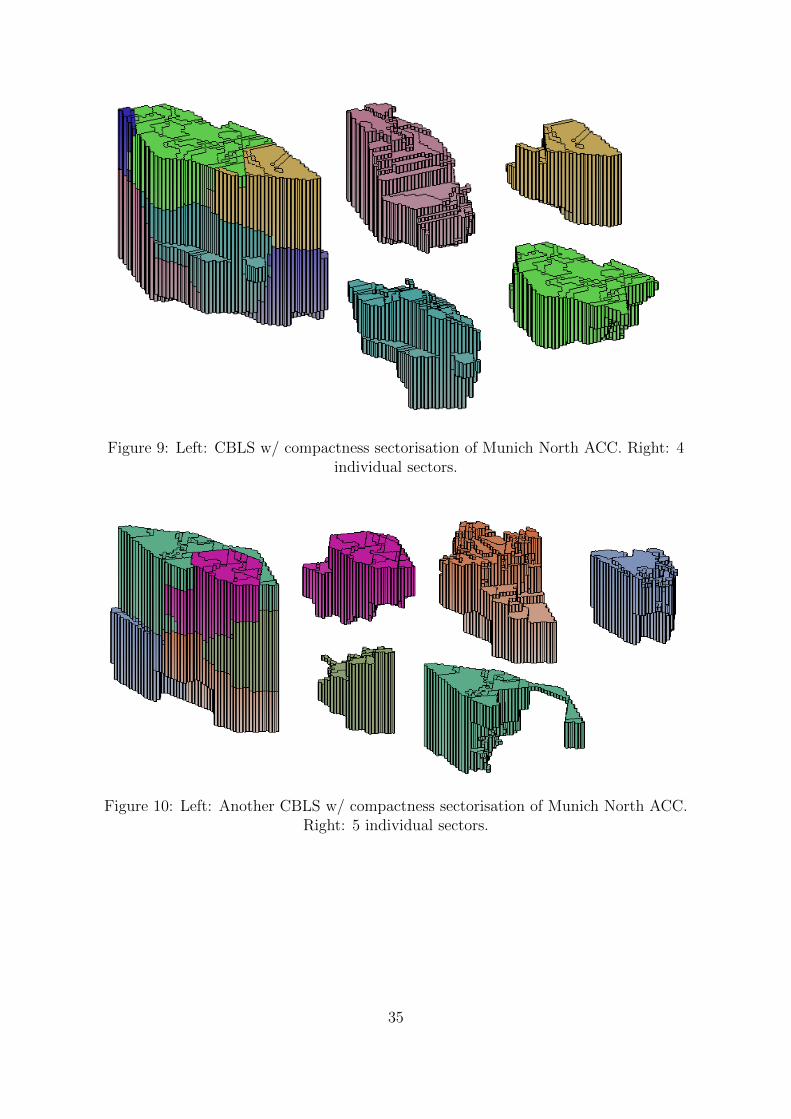
Figure 9: Left: CBLS w/ compactness sectorisation of Munich North ACC. Right: 4individual sectors.

Figure 10: Left: Another CBLS w/ compactness sectorisation of Munich North ACC.Right: 5 individual sectors.

35

Figure 11: Left: CBLS* w/ compactness sectorisation of Munich North ACC. Right: 5individual sectors, some of which were very poor.

8 Discussion

8.1 Conclusion

We have implemented a CBLS approach to airspace sectorisation using the CBLS engineof the OscaR solver, based on the constraints detailed in [3]. The resulting algorithmhas been applied on real air space data and compared against the ASTAAC sectorisationtool with regard to several relevant constraints previously outlined in [3, 4]. Finally, anattempt was made at improving the shapes resulting from our sectorisation algorithm bythe use of a Compact constraint. This yielded certain positive results, but appeared totake a toll on the effect of the other constraints in the model.

As was touched upon earlier, systematic search, while lacking the scalability of localsearch, offers completeness and optimality. For a problem of this kind, however, sub-optimal solutions can arguably be of sufficient quality for the purpose of ATC, makingthe trade-off in completeness and optimality worthwhile. We also want our sectorisationalgorithm to be able to handle possibly huge problem instances such as entire continents,which is another argument in favour of local search. There are however many othertechniques for the solving of difficult optimisation problems, and whether local search isthe best alternative among them is another issue entirely.

In OscaR.cbls, the lack of delta functions was problematic due to the fact that probingthe moves became very expensive as the number of cells grew large, unless measures weretaken to significantly narrow down the neighbourhood by various heuristics. In somecases, a delta function providing a cheap over-approximation of the impact of a givenmove is highly preferable to computing the exact delta. The compactness constraint of[3], for instance, relies on this type of estimation in order to avoid the costly Θ(|E| + |V |)time (for a graph G = 〈V,E〉 representing an airspace) operations required for measuringthe exact impact. Due to the lack of delta functions, we are not able to make such cheapapproximations, granted that the constraint itself must provide a more exact measure ofthe dissatisfaction of some condition.

36

Implementing constraints in a problem-independent fashion is something that hasproven somewhat difficult during this work. It often seems to be the case that certainmodifications have to be made depending on the characteristics of the problem and thestructure of the data.

8.2 Future Work

As was noted in Section 7.2, despite minimisation of the surface area between the sec-tors, our sectorisations still left a lot to be desired in terms of sector shapes. The Com-pact constraint of Section 4.2.6 remains to be implemented. Such a constraint wouldlikely provide a more reliable measure of compactness, and provides a penalty that canbe minimised near to zero, which was not the case for the simplistic Compact constraintin this thesis.

We speculate that in order to further speed up the search algorithm, it may notbe necessary to compute the most improving move in each iteration. Rather, a searchprocedure might compute the j most improving moves and perform them one by one,before computing the next set of j moves, where the value of j would have to be tunedexperimentally.

CBLS in general appears to be a well-suited alternative for airspace sectorisation.Due to the flexible manner in which constraints are handled, our algorithm can easily beconfigured to satisfy other constraints as they become of interest.

37

References

[1] Krzysztof R. Apt. Principles of Constraint Programming. Cambridge UniversityPress, 1999.

[2] Nicolas Beldiceanu, Mats Carlsson, and Jean-Xavier Rampon. Global constraintcatalogue: Past, present, and future. Constraints, 12(1):21–62, March 2007. The cur-rent working version of the catalogue is at http://www.emn.fr/z-info/sdemasse/aux/doc/catalog.pdf.

[3] P. Flener and J. Pearson. Propagators and violation functions for geometric andworkload constraints arising in airspace sectorisation. Technical Report 1401.7463,Computing Research Repository, January 2014. Available at http://arxiv.org/

abs/1401.7463.

[4] Pierre Flener and Justin Pearson. Automatic airspace sectorisation: A survey. Tech-nical Report 1311.0653, Computing Research Repository, November 2013. Availableat http://arxiv.org/abs/1311.0653.

[5] Holger H. Hoos and Thomas Stutzle. Stochastic Local Search - Foundations andApplications. Morgan Kaufmann, June 2004.

[6] Lester Ingber. Adaptive simulated annealing (ASA): Lessons learned. Control andCybernetics, 1995.

[7] Peter Jagare. Airspace sectorisation using constraint programming. Master’sthesis, Uppsala University, Sweden, Report IT 11 021, Faculty of Science andTechnology, 2011. Available at http://urn.kb.se/resolve?urn=urn:nbn:se:uu:

diva-155783.

[8] Peter Jagare, Pierre Flener, and Justin Pearson. Airspace sectorisation usingconstraint-based local search. In Sabrina Saunders-Hodge and Colin Meckiff, edit-ors, ATM 2013, the 10th USA / Europe Seminar on Air Traffic Management R&D,Chicago, Illinois, USA, 2013. Best paper of theme: Network and Strategic TrafficFlow Optimization.

[9] Renaud De Landtsheer. OscaR.cbls: a constraint-based local search engine. Avail-able at https://bitbucket.org/oscarlib/oscar/downloads/Oscar.cbls.pdf.

[10] Michael J. Maher. Analysis of a global contiguity constraint. In Workshop onRule-Based Constraint Reasoning and Programming, held at CP 2002, the 8th Inter-national Conference on Principles and Practice of Constraint Programming, 2002.

[11] J.P. May. A Concise Course in Algebraic Topology. Chicago Lectures in Mathemat-ics. University of Chicago Press, 1999.

[12] OscaR Team. OscaR: Scala in OR, 2012.Available from https://bitbucket.org/oscarlib/oscar.

38

[13] Gilles Pesant and Jean-Charles Regin. SPREAD: A balancing constraint based onstatistics. In Peter van Beek, editor, CP 2005, the 11th International Conference onPrinciples and Practice of Constraint Programming, volume 3709 of LNCS, pages460–474. Springer, 2005.

[14] Pierre Schaus, Yves Deville, and Pierre Dupont. Bound-consistent deviation con-straint. In Christian Bessiere, editor, CP 2007, the 13th International Conferenceon Principles and Practice of Constraint Programming, volume 4741 of LNCS, pages620–634. Springer, 2007.

[15] Ronald L. Rivest Thomas H. Cormen, Charles E. Leiserson and Clifford Stein. In-troduction to Algorithms, 3rd edition. The MIT Press, 2009.

[16] Pascal Van Hentenryck and Laurent Michel. Constraint-Based Local Search. TheMIT Press, 2005.

[17] Hakon Wadell. Volume, shape, and roundness of quartz particles. The Journal ofGeology, 43(3):250–280, April/May 1935.

39