Airports, Air Pollution, and Contemporaneous...
42
Review of Economic Studies (2016) 83, 768–809 doi:10.1093/restud/rdv043 © The Author 2015. Published by Oxford University Press on behalf of The Review of Economic Studies Limited. Advance access publication 20 October 2015 Airports, Air Pollution, and Contemporaneous Health WOLFRAM SCHLENKER Columbia University and NBER and W. REED WALKER University of California at Berkeley and NBER First version received November 2012; final version accepted July 2015 (Eds.) We link daily air pollution exposure to measures of contemporaneous health for communities surrounding the twelve largest airports in California. These airports are some of the largest sources of air pollution in the US, and they experience large changes in daily air pollution emissions depending on the amount of time planes spend idling on the tarmac. Excess airplane idling, measured as residual daily taxi time, is due to network delays originating in the Eastern US. This idiosyncratic variation in daily airplane taxi time significantly impacts the health of local residents, largely driven by increased levels of carbon monoxide (CO) exposure. We use this variation in daily airport congestion to estimate the population dose- response of health outcomes to daily CO exposure, examining hospitalization rates for asthma, respiratory, and heart-related emergency room admissions. A one standard deviation increase in daily pollution levels leads to an additional $540 thousand in hospitalization costs for respiratory and heart-related admissions for the 6 million individuals living within 10 km (6.2 miles) of the airports in California. These health effects occur at levels of CO exposure far below existing Environmental Protection Agency mandates, and our results suggest there may be sizable morbidity benefits from lowering the existing CO standard. Key words: Health effects of pollution, Airport congestion, Network delays, Instrumental variables. JEL Codes: Q53, J1, C26 The effect of pollution on health remains a highly debated topic. The US Clean Air Act (CAA) requires the Environmental ProtectionAgency (EPA) to develop and enforce regulations to protect the general public from exposure to airborne contaminants that are known to be hazardous to human health. In January 2011, the EPA decided against lowering the existing CAA carbon monoxide standard due to insufficient evidence that relatively low carbon monoxide (CO) levels adversely affect human health. In order to assess the benefits of lowering the standard, accurate estimates are needed that link contemporaneous air pollution exposure to observable health outcomes at levels of pollution currently faced by local populations. However, these estimates are hard to come by as pollution is rarely randomly assigned across individuals, and individuals who live in areas of high pollution may be in worse health for reasons unrelated to pollution. Preferences for clean air may covary with unobservable determinants of health (e.g. exercise), which can lead to various forms of omitted variable bias in regression analysis. Moreover, heterogeneity 768 Downloaded from https://academic.oup.com/restud/article-abstract/83/2/768/2461206 by University of Toronto user on 16 March 2018
Transcript of Airports, Air Pollution, and Contemporaneous...

[17:34 10/3/2016 rdv043.tex] RESTUD: The Review of Economic Studies Page: 768 768–809
Review of Economic Studies (2016) 83, 768–809 doi:10.1093/restud/rdv043© The Author 2015. Published by Oxford University Press on behalf of The Review of Economic Studies Limited.Advance access publication 20 October 2015
Airports, Air Pollution, andContemporaneous Health
WOLFRAM SCHLENKERColumbia University and NBER
and
W. REED WALKERUniversity of California at Berkeley and NBER
First version received November 2012; final version accepted July 2015 (Eds.)
We link daily air pollution exposure to measures of contemporaneous health for communitiessurrounding the twelve largest airports in California. These airports are some of the largest sources ofair pollution in the US, and they experience large changes in daily air pollution emissions depending onthe amount of time planes spend idling on the tarmac. Excess airplane idling, measured as residual daily taxitime, is due to network delays originating in the Eastern US. This idiosyncratic variation in daily airplanetaxi time significantly impacts the health of local residents, largely driven by increased levels of carbonmonoxide (CO) exposure. We use this variation in daily airport congestion to estimate the population dose-response of health outcomes to daily CO exposure, examining hospitalization rates for asthma, respiratory,and heart-related emergency room admissions. A one standard deviation increase in daily pollution levelsleads to an additional $540 thousand in hospitalization costs for respiratory and heart-related admissionsfor the 6 million individuals living within 10 km (6.2 miles) of the airports in California. These healtheffects occur at levels of CO exposure far below existing Environmental Protection Agency mandates, andour results suggest there may be sizable morbidity benefits from lowering the existing CO standard.
Key words: Health effects of pollution, Airport congestion, Network delays, Instrumental variables.
JEL Codes: Q53, J1, C26
The effect of pollution on health remains a highly debated topic. The US Clean Air Act (CAA)requires the Environmental ProtectionAgency (EPA) to develop and enforce regulations to protectthe general public from exposure to airborne contaminants that are known to be hazardous tohuman health. In January 2011, the EPA decided against lowering the existing CAA carbonmonoxide standard due to insufficient evidence that relatively low carbon monoxide (CO) levelsadversely affect human health. In order to assess the benefits of lowering the standard, accurateestimates are needed that link contemporaneous air pollution exposure to observable healthoutcomes at levels of pollution currently faced by local populations. However, these estimates arehard to come by as pollution is rarely randomly assigned across individuals, and individuals wholive in areas of high pollution may be in worse health for reasons unrelated to pollution. Preferencesfor clean air may covary with unobservable determinants of health (e.g. exercise), which canlead to various forms of omitted variable bias in regression analysis. Moreover, heterogeneity
768
Downloaded from https://academic.oup.com/restud/article-abstract/83/2/768/2461206by University of Toronto useron 16 March 2018

[17:34 10/3/2016 rdv043.tex] RESTUD: The Review of Economic Studies Page: 769 768–809
SCHLENKER & WALKER AIRPORTS AND AIR POLLUTION 769
across individuals in either preference for, or health responses to, ambient air pollution impliesthat individuals may self-select into locations on the basis of these unobserved differences. Inboth cases, estimates of the health effects of ambient air pollution may reflect the response ofvarious subpopulations and/or spurious correlations pertaining to omitted variables. While recentresearch attempts to address the issue of non-random assignment using various econometrictools such as fixed effects or instrumental variables, these studies often focus on infant healthover longer periods of time (Chay and Greenstone, 2003; Currie and Neidell, 2005). Much lessis known about short-term, daily effects of ambient air pollution on the health of the more generalpopulation, such as the non-elderly, non-child, adult population.1
We develop a framework for estimating the contemporaneous effect of air pollution on healthusing variation in local air pollution driven by airport runway congestion. Airports are one of thelargest sources of air pollution in the US with Los Angeles International Airport (LAX) being thelargest source of carbon monoxide in the state of California (Environmental Protection Agency,2005). A large fraction of airport emissions come from airplanes, with the largest aggregatechannel of emissions stemming from airplane idling (Transportation Research Board, 2008). Weshow that airport runway congestion, as measured by the total time planes spent taxiing betweenthe gate and the runway, is a significant predictor of local pollution levels. Since local runwaycongestion may be correlated with other determinants of pollution such as weather, we exploitthe fact that California airport congestion is driven by network delays that began in large airportsoutside of California.2 A recent article in the New York Times (New York Times 27 January,2012) provides a useful motivation:
[Airplane] delays ripple across the country. A third of all delays around the nation eachyear are caused, in some way, by the New York airports, according to the F.A.A. Or, asPaul McGraw, an operations expert with Airlines for America, the industry trade group,put it, ‘When New York sneezes, the rest of the national airspace catches a cold’.
Our analysis hence links health outcomes of residents living near California airports to changes inair pollution driven by runway congestion at airports on the East Coast. The identifying variationin California pollution is caused by events several thousand miles away (e.g. weather in Atlanta),which is unlikely to be correlated with determinants of health in California.
The goal of this article is to identify the ways in which short run, daily variation in air pollutionaffects population health. In doing so, this article makes four primary contributions to the existingliterature in this area. First, while most existing literature focuses on the health impacts of infantsor elderly, we are able to examine the health responses of the entire population. We find that
1. There is a larger literature in epidemiology which focuses on daily responses to air pollution (see e.g. Ito et al.(2007), Linn et al. (1987), Peel et al. (2005), Schildcrout et al. (2006), Schwartz et al. (1996)). The work in our articlecomplements the existing epidemiological literature by focusing on issues pertaining to measurement error, avoidancebehaviour, and self-selection bias in the context of susceptibility to pollution exposure. Each of these issues is criticallyimportant to providing unbiased estimates of the causal relationship between pollution and health. The instrumentalvariables approach in this article exploits arguably exogenous pollution shocks that are unlikely to be known by localresidents, allowing us to simultaneously address issues of measurement error and avoidance behaviour. Recent workin economics and environmental health, discussed in more detail below, suggests that short run variation in pollutionexposure may be significant predictors of mortality and morbidity (Moretti and Neidell, 2011; Knittel et al., 2011).
2. This relationship is well known within the transportation literature (Welman et al., 2010). Optimal airplanescheduling incorporates anticipated ripple effect. For example, Pyrgiotisa et al. (2013) use queuing theory to simulatehow delays propagate through the system. They quote a study that found a multiplier effect of seven, i.e., each 1-hourdelay of a particular airplane leads to a combined 7 hours delay for the airline.
Downloaded from https://academic.oup.com/restud/article-abstract/83/2/768/2461206by University of Toronto useron 16 March 2018

[17:34 10/3/2016 rdv043.tex] RESTUD: The Review of Economic Studies Page: 770 768–809
770 REVIEW OF ECONOMIC STUDIES
infants as well as the elderly are most sensitive to ambient air pollution. At the same time, a one-unit increase in pollution has much larger aggregate effects for adults aged 20–64 years, giventheir large share of the overall population. Studies that focus on infants or the elderly significantlyunderestimate overall health effects.
The second contribution of this article is to estimate the contemporaneous effect of multiplepollutants simultaneously. It has traditionally been difficult to decipher which pollutant isresponsible for adverse health outcomes since short-term fluctuations among ambient airpollutants are highly correlated. Our solution to this identification problem is to rely on the factthat wind speed and wind direction transport individual pollutants in different ways. By usinginteractions between taxi time, wind speed, and wind angle from airports, we can pin down thedirect effect of each pollutant, while holding the others constant. We use over-identified models toinstrument for several pollutants simultaneously, an approach that was simultaneously developedin related work by Knittel et al. (2011). We find that CO is responsible for the majority of theobserved increase in hospital admissions, although we cannot rule out that this may be driven byother unobserved pollutants that are correlated with airplane-driven CO emissions. This findinghas direct policy implications. The EPA recently decided to maintain the current CO pollutionstandard, citing a lack of evidence that reducing CO below current ambient levels would improvepopulation health outcomes.
We believe there are two additional features that set this article apart from existing workin both economics and epidemiology. Our article is most closely related to the recent workof Moretti and Neidell (2011) and Knittel et al. (2011) who also instrument daily pollutionin health regressions with variation in local transportation conditions (i.e. container shippingin Long Beach, CA, and automobile congestion in Central and Southern CA, respectively).Relative to these article and the existing literature, we believe this paper is the first to use thenetwork structure of transportation to generate local variation in congestion that is driven byevents that occur several thousand miles away. This matters because one of the key drivers oftransportation congestion is local weather, and local weather is also likely to affect ambientpollution, violating the identifying assumptions of the model. By way of example, we show thatinstrumenting local airport congestion with network delays that are not correlated with localweather doubles our point estimates, relative to the baseline case. We also explicitly modelthe spatial dispersion of air pollution emissions, as it varies with wind speed, wind direction,and distance from the airport. Pollutant transport is very locally heterogeneous, and failing toaccount for this spatial heterogeneity leads to bias when estimating the population dose-responsefunction.
The fourth contribution of this study is the use of newly available Emergency Discharge Datato better capture the morbidity impacts of air pollution. Previous research has predominantlyfocused on the effects of pollution on mortality or morbidity as measured in InpatientDischarge Records. Inpatient Discharge data consist only of observations for patients that stayedovernight in a hospital, and thus exclude a large fraction of respiratory-related emergency roomadmissions that do not require overnight hospital visits. We show that estimates using the morecommonly used Inpatient Discharge data substantially underestimate the morbidity impacts of airpollution, relative to estimates from the combined Emergency Discharge and Inpatient Dischargedatasets.3
In summary, our approach combines newly available data with arguably exogenous dailychanges in air pollution that originate several thousand miles away and are unknown to the
3. Knittel et al. (2011) focus on infant mortality, while Moretti and Neidell (2011) examine morbidity outcomes,but only for individuals of Emergency Room visits that eventually get admitted to an overnight stay as the authors relyon the Inpatient Discharge data.
Downloaded from https://academic.oup.com/restud/article-abstract/83/2/768/2461206by University of Toronto useron 16 March 2018

[17:34 10/3/2016 rdv043.tex] RESTUD: The Review of Economic Studies Page: 771 768–809
SCHLENKER & WALKER AIRPORTS AND AIR POLLUTION 771
local population. The instrumental variables setting allows us to simultaneously address issuespertaining to both avoidance behaviour and classical forms of measurement error, each ofwhich lead to significant downward bias in conventional dose-response estimates. The primaryestimation framework examines how zip code level emergency room admissions covary withthese quasi-experimental increases in air pollution stemming from airports.
We find that a one standard deviation increase in daily pollution explains roughly one thirdof average daily admissions for asthma problems. It leads to an additional $540 thousand perday in hospitalization costs for respiratory and heart related admissions of individuals within10 km of one of the twelve largest airports in California. This is likely a significant lower boundof the social costs as the willingness to pay to avoid a sickness might be significantly largerthan the medical reimbursement cost (Grossman, 1972). Our baseline IV estimates are an orderof magnitude larger than uninstrumented fixed effects estimates, highlighting the importance ofaccounting for measurement error and/or avoidance behaviour in conventional estimators. Wefind no evidence that airport runway congestion affects diagnoses unrelated to air pollution suchas bone fractures, stroke, or appendicitis. We also present a variety of evidence in favour of anon-linear dose-response function. As pollution levels increase the marginal effect of a 1 unitincrease in pollution increases but at a decreasing rate. This is consistent with thresholds at whichthe health effect of air pollution levels off (i.e. the dose-response function is not convex overthe levels of pollution we observe), and along the lines of what research in epidemiology hasobserved (Pope et al., 2009; Pope III et al., 2011).
We present several sensitivity checks of results that do not alter our conclusions. For example,we focus on morning airport congestion in the East since it is possible that California airport delaysimpact airports on the East Coast, which then feedback to California airports. Due to the differencein time zones, very few flights from California reach East Coast airports before 12 pm. Estimatesremain similar to our baseline estimates. A distributed lag model finds no evidence for delayedimpacts or forward displacement, i.e., that individuals on the brink of an asthma or heart attackmay experience an episode that would have otherwise occurred in the next few days anyway.A Poisson model linking sickness counts to pollution levels gives comparable estimates to ourbaseline linear probability model, which does not account for the truncation of daily sicknessrates at zero. Finally, we find little evidence of treatment effect heterogeneity that would raiseconcerns pertaining to forms of self-selection bias and/or the external validity of the underlyingdose-response estimates.
The findings in this article suggest that daily variation in ambient air pollution haseconomically significant health effects at levels below current EPA mandates, at least for thepopulation that comprises our study. We believe this is particularly important due to the factthat in January 2011, the EPA decided against lowering the existing CAA CO standard due toinsufficient evidence that relatively low CO levels adversely affect human health. The maximumhourly CO concentration in our data is 7.5 ppm (see Supplementary Table A2), which is belowthe ambient air quality standard of 35 ppm for any 1-hour reading or 9 ppm for any 8-houraverage, i.e., air quality levels were always within the limit.4 Yet, fluctuations in pollution levelssignificantly below the standard still have sizable health consequences. While a full-fledgedbenefit–cost analysis would have to balance the cost of reducing CO against the benefits, EPAindicated there were no appreciable benefits from lowering the standard to begin with, which wefind not to be the case.
4. The same is not true for NO2. The maximum 1-hour reading in our data is 136 ppb, which is above the 1-hourstandard of 100 ppb.
Downloaded from https://academic.oup.com/restud/article-abstract/83/2/768/2461206by University of Toronto useron 16 March 2018

[17:34 10/3/2016 rdv043.tex] RESTUD: The Review of Economic Studies Page: 772 768–809
772 REVIEW OF ECONOMIC STUDIES
1. BACKGROUND: AIRPORTS, AIRPLANES, AND AIR POLLUTION
Regulators have long been aware of the pollution generated by cars, trucks, and public transit.There have been countless legislative policies designed to curtail harmful emissions from thesesources (Auffhammer and Kellogg, 2011). However, aircraft and airport emissions have onlyrecently become the subject of regulatory scrutiny, although little has been done to reduce ormanage emissions generated by airports and air travel. While there has been some effort to curtailthe substantial CO2 emissions generated by aircraft,5 there has been relatively little effort tocontrol or contain some of the more pernicious air pollutants generated by jet engines. This lackof regulatory scrutiny can be traced back to the way in which pollutants are regulated in theUS under the Clean Air Act. Current Federal law preempts all federal, state, and local agenciesexcept the Federal Aviation Administration from establishing measures to reduce emissions fromaircraft due to potential interstate and international commerce conflicts that might arise fromother decentralized regulations.6
Aircraft jet engines, like many other mobile sources, produce carbon dioxide (CO2), nitrogenoxides (NOx), carbon monoxide (CO), oxides of sulphur (SOx), unburned or partially combustedhydrocarbons (also known as volatile organic compounds, or VOCs), particulates, and othertrace compounds (Federal Aviation Administration, 2005). Each of these pollutants is emittedat different rates during various phases of operation, such as idling, taxing, takeoff, climbing,and landing. NOx emissions are higher during high power operations like takeoff whencombustor temperatures are high. On the other hand, CO emissions are higher during low poweroperations like taxiing when combustor temperatures are low and the engine is less efficient(Federal Aviation Administration, 2005).7 Even though the aircraft engine is often idling duringtaxi-out, the per minute CO and NOx emissions factors are higher than at any other stage of aflight (Environmental Protection Agency, 1992). Combining this with the long duration of taxi-out times during peak periods of the day, total taxiing over the course of a day can add up to asubstantial amount. Consistent with these facts, Los Angeles International airport is estimated tobe the largest point source of CO emissions in the state of California, the second largest of NOx ,the twenty-ninth largest of SO2, and the 2,763 and 2,782 largest of PM10 and PM2.5, respectively(Environmental Protection Agency, 2005).
Airports provide a particularly compelling setting through which to estimate the contempo-raneous relationship between air pollution and health. Not only are airports some of the largestpolluters of ambient air pollution in the US but they also have extraordinarily rich data on dailyoperating activity, detailing for each domestic flight the length of time spent taxiing to and fromthe gate before takeoff and after landing. This allows for a precise understanding of the aggregateamount of daily runway congestion at airports. Moreover, daily runway congestion at airportsexhibits a great degree of residual variation even after controlling for normal scheduling patterns.Much of the variation in runway congestion is driven by network delays propagating from majorairport hub delays thousands of miles away. Network delays at distant airports serve as an idealinstrumental variable for local pollution; the effect of a snow storm in Chicago on congestion atLAX should be orthogonal to any other confounding influences of air pollution in the LosAngeles
5. The European Union has recently approved greenhouse gas measures, which oblige airlines, regardless ofnationality, that land or take off from an airport in the European Union to join the emissions trading system starting on1 January, 2012.
6. Currently, the EPA has an agreement with the FAA to voluntarily regulate ground supportequipment at participating airports known as the Voluntary Airport Low Emission (VALE) program(United States Environmental Protection Agency, 2004).
7. As a result, reducing engine power for a given operation like takeoff or climb out generally increases the rateof CO emissions and reduces the rate of NOx emissions.
Downloaded from https://academic.oup.com/restud/article-abstract/83/2/768/2461206by University of Toronto useron 16 March 2018

[17:34 10/3/2016 rdv043.tex] RESTUD: The Review of Economic Studies Page: 773 768–809
SCHLENKER & WALKER AIRPORTS AND AIR POLLUTION 773
area. In addition, local residents are likely unaware of increases in taxi time and hence cannotengage in self-protective behaviour. Finally, every airport has detailed weather data, allowingresearchers to exploit the spatial distribution of airport-generated pollution. We can thereforeestimate how areas downwind of an airport on a given day are disproportionately affected byrunway congestion relative to areas upwind. Understanding this spatial variation in pollutanttransport improves the efficiency of our estimates, while also providing important tests of thevalidity of our research design.
2. DATA
This project uses the most comprehensive data currently available on airport traffic, air pollution,weather, and daily measures of health in California. These data are rich in both temporal andspatial dimension, allowing for fine-grained analysis of how daily airport congestion impactsareas downwind of an airport on a given day. The various datasets and linkages are described inmore detail below.
2.1. Airport traffic data
A useful feature of a study involving airports is the detailed nature of daily flight data. The Bureauof Transportation Statistics (BTS) Airline On-Time Performance Database contains flight-levelinformation by all certified US air carriers that account for at least 1% of domestic passengerrevenues. It has a wealth of information on individual flights: flight number, the origin anddeparture airport, scheduled departure and arrival times, actual departure and arrival times, thetime the aircraft left the runway and when it touches down. We construct a daily congestionmeasure for each of the twelve major airports in California by aggregating the combined taxi timeof all airplanes at an airport. This measure consists of (1) the time airplanes spend between leavingthe gateway and taking off from the runway and (2) the time between landing and reaching thegate. An interesting feature of aggregate daily taxi time is the large amount of residual variationremaining after controlling for daily airport scheduling, weather, and holidays. We relate thisvariation to local measures of pollution and health in our econometric analysis. One caveat ofthe BTS data is that it only includes information for major domestic airline passenger travel.8
As long as international flights are not treated differently in the queuing system and are hencecolinear to the taxi time of domestic flights, congestion of national flights should be a good proxyfor overall congestion.
We limit our analysis to the twelve largest airports in California by passenger count. Theseairports are in alphabetical order (including airport call sign in brackets): Burbank (BUR),Los Angeles International (LAX), Long Beach (LGB), Oakland International (OAK), OntarioInternational (ONT), Palm Springs (PSP), San Diego International (SAN), San FranciscoInternational (SFO), San Jose International (SJC), Sacramento International (SMF), Santa Barbara(SBA), and SantaAna / Orange County (SNA). The locations of these airports are shown as dots inFigure 1.Average flight statistics at each of these airports are reported in Supplementary Table A1.There is significant variation in daily ground congestion at airports: the standard deviation of dailytaxi time at the largest airport (LAX) is 1,852 minutes. Once we account for year, month, weekdayand holiday fixed effects as well as local weather, the remaining variation is still 891 minutes.Most of the airports are close to urban areas as they serve the travel needs of these populations.
8. In January 2005, international departures (both cargo and passenger) accounted for 8.5% of total departures,whereas cargo (both international and domestic) accounted for 5.9% of all US airport departures (Department ofTransportation, 2009).
Downloaded from https://academic.oup.com/restud/article-abstract/83/2/768/2461206by University of Toronto useron 16 March 2018

[17:34 10/3/2016 rdv043.tex] RESTUD: The Review of Economic Studies Page: 774 768–809
774 REVIEW OF ECONOMIC STUDIES
Figure 1
Location of airports, pollution monitors, and zip codes.
Notes: The 12 largest airports in California are shown as dots. The location of CO pollution monitors in the California AirResource Board (CARB) data base are shown as x, the location of NO2 monitors as +. Zip code boundaries are shown ingrey. They are shaded if the centroid is within 10 km (6.2 miles) of an airport.
Seven airports in California rank among the top fifty busiest airports in the nation according topassenger enplanement (Federal Aviation Administration, 2009).
A potential concern when linking daily airport activity to daily ambient air pollution levels isthat runway congestion in California airports may be highest in the late afternoon and evening.This would lead us to erroneously misclassify some of the daily airport effects to the wrong day.Supplementary Figure A2 plots the distribution of aggregate taxi time within a day. Most groundactivity at airports is skewed towards the beginning of the day. We will address the sensitivity
Downloaded from https://academic.oup.com/restud/article-abstract/83/2/768/2461206by University of Toronto useron 16 March 2018

[17:34 10/3/2016 rdv043.tex] RESTUD: The Review of Economic Studies Page: 775 768–809
SCHLENKER & WALKER AIRPORTS AND AIR POLLUTION 775
of our estimates towards these issues of misclassification or across-day spillovers in subsequentsections.
2.2. Pollution data
We construct daily measures of air pollution surrounding airports using the monitoring networkmaintained by the California Air Resource Board (CARB). This database combines pollutionreadings for all pollution monitors administered by CARB, including information on the exactlocation of the monitor. Data includes both daily and hourly pollution readings. We concentrateon the set of monitors with hourly emission readings for CO, NO2, and O3 in the years 2005–7.9
The locations of all CO and NO2 monitors in relation to airports are shown in Figure 1.A unique feature of pollution data is the significant number of missing observations in the
database. We therefore use the following algorithm when we aggregate the hourly data to dailypollution readings: Our measure of the daily maximum pollution reading is simply the maximumof all hourly pollution readings. The daily mean is the duration-weighted average of all hourlypollution readings. We define the duration as the number of hours until the next reading.10 Weprefer this approach to simply taking the arithmetic average of all hourly readings on a day sincehourly pollution data exhibit great temporal dependence. A missing hourly observation is betterapproximated by the previous non-missing value than the daily average. We also keep track ofthe number of observations per day. In a sensitivity check (not reported) we rerun the analysisusing only monitors with at least 20 or 12 readings per day.11
We create daily zip code pollution measures by taking the average monitor readingof all monitors within 15 km of a zip code centroid, weighting by the inverse distancebetween the monitor and the zip code centroid.12 Summary statistics are given in Panel A ofSupplementary Table A2. Since we have both the longitude and latitude of all airports and zipcode centroids, we are able to derive (1) the distance between the airport and a zip code, and (2)the angle at which the zip code is located relative to the airport. In order to leverage the spatialfeatures of our data, we normalize the angle between a zip code centroid and an airport to 0 if thezip code is lying to the north of the airport. Degrees are measured in clockwise fashion, e.g. a zipcode that is directly east of an airport will have an angle of 90◦. The angle between an airportand a zip code allows us to explore the link between airport emissions and pollution downwindof airports using the weather data described next.
9. While data exist for other pollutants in California, we limit our analysis to using CO, NO2 as they are directlyemitted by airplanes and have better coverage than PM10. O3 forms from VOC and NOx . In a sensitivity check we donot find that O3 pollution levels are impacted by airport congestion. Nevertheless, we present sensitivity analyses thatinclude O3 and PM10 as controls with little effect on our results. While monitor data exists as far back as 1993, portionsof our hospital data, described further in this section, exists only from 2005 onwards.
10. Readings occur on the hour of each day ranging from midnight to 11 pm. If readings at the beginning of a day(midnight, 1 am, etc.) are missing, we adjust the duration of the first reading from midnight to the second reading. Forexample, if readings occur on 3 am, 5 am, and 8 am, the 3 am reading would be assigned a duration of 5 hours and the5 am reading would be assigned a duration of 3 hours. By the same token, if the last reading of a day is not 11pm, theduration of that last reading is from the time of the reading until midnight.
11. If a monitor has not a single reading for a day, we approximate its value in a three step procedure: (1) we derivethe cumulative density function (cdf) at each monitor; (2) take the inverse-distance weighted average of the cdf for a givenday at all monitors with non-missing data; (3) we fill the missing observation with the same percentile of the station’scdf. For example, if surrounding monitors with non-missing data on average have pollution levels that correspond to the80th percentile of their respective distributions, we fill the missing value of a station with the 80th percentile of its owndistribution of pollution readings. This procedure gives us a balanced panel.
12. Inverse distance weighting pollution measures has been used to impute pollution in previous research. See forexample, Currie and Neidell (2005).
Downloaded from https://academic.oup.com/restud/article-abstract/83/2/768/2461206by University of Toronto useron 16 March 2018

[17:34 10/3/2016 rdv043.tex] RESTUD: The Review of Economic Studies Page: 776 768–809
776 REVIEW OF ECONOMIC STUDIES
2.3. Weather data
We use temperature, precipitation, and wind data in our analysis to both control for the directeffects of weather on health (Deschênes et al., 2009) and also to leverage the quasi-experimentalfeatures of wind direction and wind speed in distributing airport pollution from airports. Ourweather data comes from Schlenker and Roberts (2009), which provides minimum and maximumtemperature as well as total precipitation at a daily frequency on a 2.5×2.5 mile grid for the entireUS.13 To assign daily weather observations to an airport or zip code, we use the grid cell in whichthe zip code centroid is located. Summary statistics for the zip-code level data are given in PanelB of Supplementary Table A2.
Average wind speed and wind direction come from the National Climatic Data by the NationalOceanic and Atmospheric Administration’s (NOAA) hourly weather stations. Most airports haveweather stations with hourly readings. We construct wind direction, which is normalized to equalzero if the wind is ‘blowing’ northward and counted in clockwise fashion. If the angles of the zipcode and the wind direction are identical, the zip code is hence exactly downwind from the airport.An angle of 180◦ implies that the zip code is upwind from the airport. The hourly wind speedand wind direction is aggregated to the daily level by calculating the duration-weighted averagebetween readings comparable to the pollution data above. The distribution of wind directions isshown in Figure 2. Airports at the ocean predominantly have winds coming from the direction ofthe ocean. For example, Santa Barbara, located on the only portion of the California coast thatruns east–west has winds blowing northward. Note again that we are measuring the directionin which the wind is blowing, not from which it is coming. In our empirical analysis, we usethis daily variation in wind speed and wind direction to predict how pollution from airportsdisproportionately impacts some zip codes more than others on a given day.
2.4. Hospital discharge and emergency room data
Health effects are measured by overnight hospital admission and emergency room visits to anyhospital in the state of California. We use the California Emergency Department & AmbulatorySurgery data set for the years 2005–7.14 The dataset gives the exact admission date, the zip code ofthe patient’s residence (as well as the hospital), the age of the patient, as well as the primary and upto twenty-four secondary diagnosis codes. An important limitation of the Emergency Departmentdata is that any person who visits an ER and is subsequently admitted to an overnight stay dropsout of the dataset. This is done to prevent double counting in California’s hospital admissionsrecords, as overnight hospital stays are logged in California’s Inpatient Discharge data. Therefore,we also obtained Inpatient Discharge data for all individuals who stayed overnight in a hospitalin the years 2005–7. In our baseline model, we focus on the sum of emergency room visits andovernight stays in a zip code-day to avoid non-random attrition in the ER data. Focusing only onemergency room admittance would suffer from selection bias as higher pollution levels (and moresevere health outcomes) could result in more overnight stays, yet the emergency room numberswould actually appear smaller.
We count the daily admissions of all people in a zip code who had a diagnosis code pertainingto three respiratory illnesses: asthma, acute respiratory, and all respiratory. Note that each category
13. There is one exception: in a set of regression models where we estimate the effect of airport weather on taxitime we use the closest non-missing daily weather station data from NOAA’s COOP station data set for each airport. Thisis because Schlenker and Roberts (2009) use a spatial interpolation procedure that might result in artificial correlationbetween weather data at airports due to the spatial interpolation technique.
14. The Emergency Room data was not collected prior to 2005.
Downloaded from https://academic.oup.com/restud/article-abstract/83/2/768/2461206by University of Toronto useron 16 March 2018

[17:34 10/3/2016 rdv043.tex] RESTUD: The Review of Economic Studies Page: 777 768–809
SCHLENKER & WALKER AIRPORTS AND AIR POLLUTION 777
Figure 2
Histogram of daily wind direction at airports.
Notes: Histogram of the distribution of daily directions in which the wind is blowing (2005–7). Plot is normalized to themost frequent category. The four circles indicate the quartile range. Airport locations are shown in Figure 1.
adds additional sickness counts but includes the previous. For example, asthma attacks are alsocounted in all respiratory problems. We also count heart-related problems, which Peters et al.(2001) have shown to be correlated with pollution. Finally, we include three placebos: stroke,bone fractures, and appendicitis.15 In our baseline model, we count a patient as suffering from asickness if either the primary or one of the secondary diagnosis codes lists the illness in question.
We merge the zip code level hospital data with age-specific population counts in each zipcode obtained from both the 2000 and 2010 Censuses. We use the weighted average betweenthe 2000 (weight 0.4) and 2010 (weight 0.6) counts, as the midpoint of our data is 2006. Welimit our analysis to the 164 zip codes whose centroid lies within 10 km of an airport andwhich have at least 10,000 inhabitants.16 The total population of these 164 zip codes is around6 million people, or roughly one sixth of the overall population of California at the time. Summarystatistics for the zip codes in the study are given in Panel C of Supplementary Table A2. We use
15. The exact ICD-9 codes are: asthma: [493, 494); acute respiratory: [460,479), [493,495), [500,509), [514,515),[516,520); all respiratory: [460, 520); heart problems: [410, 430); stroke [430, 439); bone fractures [800, 830); appendicitis:[540, 544).
16. The latter sample restriction excludes 0.8% of the total population that lives in a zip code whose centroid iswithin 10 km of an airport but has less than 10,000 inhabitants.
Downloaded from https://academic.oup.com/restud/article-abstract/83/2/768/2461206by University of Toronto useron 16 March 2018

[17:34 10/3/2016 rdv043.tex] RESTUD: The Review of Economic Studies Page: 778 768–809
778 REVIEW OF ECONOMIC STUDIES
these age-specific population counts to construct daily hospitalization rates for each zip code.Supplementary Table A3 provides sickness rates per 10 million inhabitants for both the entirepopulation as well as population subgroups of those over 65 years of age and under 5 yearsof age.
2.5. External validity — populations close to airports
Our analysis focuses on areas within 10 km of airports. This raises the broader question as tohow our estimated results generalize to populations outside of the 10 km airport radius. Table A4investigates this question by examining zip code characteristics from the 2000 Census. We presentthree comparisons: First, we look at zip codes that are in our sample in columns (1a)–(1c) butdivide them into zip codes whose centroids are within [0,5] km and (5,10] km of an airport.Second, we compare zip codes within 10 km of an airport versus neighbouring zip codes thatare between 10 km and 20 km of an airport in columns (2a)–(2c). Third, we compare zip codeswithin 10 km of an airport to all other zip code in California in columns (3a)–(3c).
For the first two sets of comparisons, few comparison tests are significant, roughly at a rate thatshould happen due to randomness. In other words, areas [0,5] km from an airport are comparableto areas (5,10] km or (10,20] km.17 On the other hand, the third set of comparisons shows thatareas within 10 km are not comparable to the rest of the state of California, which includes morerural areas. Zip codes closer to airports are on average more urban, more populated, wealthier, andhave higher housing prices. Therefore, we would caution against interpreting the estimated dose–response relationship as representative for the entire population at large. From the standpointof airport externalities, the population close to airports is the population of interest. Moreover,much of the air pollution regulation in the US is spatially targeted towards urban areas (i.e. thoseareas with higher degrees of ambient air pollution), and in that case, these estimates may be moreappropriate for regulatory analysis than a dose response function averaged over individuals inboth urban and rural locations.
3. EMPIRICAL METHODOLOGY
We are estimating the link between ground level airport congestion, local pollution levels, andcontemporaneous hospitalization rates for major airports in the state of California. To begin, weconsider the effects of increased levels of airport traffic congestion on local measures of pollution.
3.1. Aggregate daily taxi time and local pollution levels
Ambient air pollution is a function of the distance between a point source and the receptorlocation, as well as many other atmospheric variables including, but not limited to, wind speed,wind direction, humidity, temperature, and precipitation. To model the effects of increases inaggregate airport taxi time on pollution levels, we adopt the following additive linear regressionmodel
Model 1: pzat =α1Tat +Wzt�+weekdayt +montht +yeart +holidayt︸ ︷︷ ︸Zzt�
+νza +ezat, (1)
17. In all, 47% of Californians live in a zip code within 20 km of an airport.
Downloaded from https://academic.oup.com/restud/article-abstract/83/2/768/2461206by University of Toronto useron 16 March 2018

[17:34 10/3/2016 rdv043.tex] RESTUD: The Review of Economic Studies Page: 779 768–809
SCHLENKER & WALKER AIRPORTS AND AIR POLLUTION 779
where pollution pzat in zip code z that is paired with airport a on day t is specified as a function oftaxi time Tat and a vector of zip code level controls Zzt that include weather controls Wzt .18 Ourbaseline regressions include seventeen weather controls: a quadratic in minimum and maximumtemperature, precipitation, and wind speed (eight terms) as well as nine terms for wind directionthat are included in equation (3) below.19 To model this relationship formally, we define winddirection by the cosine of the difference between the wind direction and the direction in whichthe zip code is located. The variable will be equal to 1 in the case that the angle in whichthe wind is blowing equals the direction in which the zip code is located, and the variablewill be equal to zero when they are at a right angle (the difference is 90◦). The vector Wztincludes all possible time-varying interactions between distance, wind speed and angle (up anddownwind) to control for pollution formation not directly influenced by taxi time. We also controlfor temporal variation in pollution by including weekday fixed effects (weekdayt), month fixedeffects (montht), and year fixed effects (yeart) as well holiday fixed effects (holidayt) to limitthe influence of airport congestion outliers.20 In a sensitivity check (available upon request), weinstead include day fixed effects, i.e., one for each of the 1,095 days, and the results remain robust.Since there may be time-invariant unobserved determinants of pollution for any given zip code,all regressions include zip code fixed effects, νza. The parameter of interest is α1, which tellsus the effect of a 1,000 minute increase in aggregate daily ground congestion on local ambientair pollution levels. Increased airplane taxiing leads to an increase in airplane emissions andpresumably increases in ambient air pollution. Hence, we would expect this coefficient to bepositive.
We also estimate models similar to equation (1), where we interact taxi time (or instrumentedtaxi time) with the distance between an airport and the monitor. The idea would be to allow themarginal effect of taxi time to differ based on monitors that were closer relative to further fromthe airport. This results in the following equation:
Model 2: pzat = α1Tat +α2Tatdza +Zzt�+νza +ezat . (2)
The additional coefficient is α2. The effect of taxi time on pollution should fade out with distance,and we would hence expect this coefficient to be negative. The marginal effect of taxi time inmodel 2 is α1 +α2dza.
In a third step we also include interactions with wind direction and wind speed. The intuitionis that both wind direction and speed transport airport emissions across space. Thus, holdingspeed constant, areas downwind should be relatively more affected by aggregate daily taxi timerelative to areas upwind. To model this relationship formally, we let vat be the wind speed and czatthe cosine of the difference between the wind direction and the direction in which the zip codeis located, which can differ upwind czat >0 and downwind czat <0.21 Allowing for all possible
18. In principle, a zip code z could be paired with more that one airport a. In practice, our baseline model uses zipcodes whose centroid is within 10 km of an airport. Each zip code is assigned to exactly one airport as none is within10 km of two airports.
19. Specifically, our weather controls include the terms corresponding to α3,α4 and α6 −α12 in equation (3) withoutthe interaction with taxi time Tat . Results are robust to different functional forms of weather control variables.Additionally,we have estimated models that exclude all weather controls, and the coefficients for our primary pollutant of interest (COsee below) are not significantly affected (although the standard errors increase).
20. We include fixed effects for New Year, Memorial Day, July 4th, Labor Day, Thanksgiving, and Christmas, aswell as the three days preceding and following the holiday.
21. The cosine is 0 if the angle is 90◦, i.e., the separately estimated effect is different upwind and downwind.
Downloaded from https://academic.oup.com/restud/article-abstract/83/2/768/2461206by University of Toronto useron 16 March 2018

[17:34 10/3/2016 rdv043.tex] RESTUD: The Review of Economic Studies Page: 780 768–809
780 REVIEW OF ECONOMIC STUDIES
time-varying interactions we get:22
Model 3: pzat = α1Tat +α2Tatdza +α3TatczatI[czat>0]+α4TatczatI[czat<0]+α5Tatvat +α6TatdzaczatI[czat>0]+α7TatdzaczatI[czat<0]+α8Tatdzavat +α9TatczatI[czat>0]vat +α10TatczatI[czat<0]vat
+α11TatdzaczatI[czat>0]vat +α12TatdzaczatI[czat<0]vat
+Zzt�+νza +ezat . (3)
The new coefficients are α3 through α12. The predicted signs of these coefficients are less intuitive.While higher wind speeds can clear the air they may also carry greater amounts of the pollutantfurther distances.23 Moreover, downwind areas should have higher pollution levels relative tothose areas upwind, but aircrafts usually start against the wind. To better interpret the combinationof all of these interactions, we plot the marginal effects of this particular regression model usingcontour plots in subsequent sections. These contour plots provide strong visual evidence of therelationship between daily aggregate airport taxi time, wind speed, wind direction, and localpollution levels.
One potential cause for concern in equations (1)–(3) are any omitted transitory determinantsof local pollution levels that may also covary with ground congestion. If such omitted variablesexist, then least squares estimates of the coefficients on taxi time (e.g. α1) will be biased. Thiscould occur, for example, if weather adversely affected airport activity while also affecting localpollution levels. To address this potential source of bias, we need an instrumental variable thatis correlated with changes in ground congestion at an airport but is unrelated to local levelsof pollution. A natural instrument comes from delays at major airport hubs outside California,which propagate through the air network as connecting flights are delayed, leading to moreground congestion at airports in California. The basic logic is that instead of smoothing outscheduling over the course of the day, planes now arrive in more distinct blocks of time, leadingto more waiting/taxiing by those planes taking off as the runway space is shared. Specifically,we instrument taxi time at each California airport with taxi time at major airports outside ofCalifornia (Atlanta (ATL), Chicago O’Hare (ORD), and New York John F. Kennedy (JFK)), inthe following first stage regression:24
Tat = αa0 +3∑
k=1
12∑a=1
αakTktIa +Zat�+ωat . (4)
Supplementary Figure A1 shows the location of those airports in relation to the California airports.We allow the coefficients αak in equation (4) to vary by airport a by interacting taxi time withan airport indicator Ia. These interactions allow for heterogeneity in the impact of delays frommajor airports outside of California Tkt on each of the California airports Tat . This is important
22. The exact dispersion of pollution depends on additional factors like acceleration and height of emissions.Benson (1984) presents a formal model of pollution dispersion around roads that includes many variables we do notobserve. The standard in the literature has hence been to estimate reduced-form relationship with wind direction andspeed (Batterman et al., 2010).
23. Recall that we are already controlling for overall wind speed in Wzt , but it has so far not been interacted withtaxi time or any other weather measure.
24. These airports were chosen because they are among the largest airports in the country, they serve differentregions, and they are subject to different weather systems. The results are robust to different airport specifications.
Downloaded from https://academic.oup.com/restud/article-abstract/83/2/768/2461206by University of Toronto useron 16 March 2018

[17:34 10/3/2016 rdv043.tex] RESTUD: The Review of Economic Studies Page: 781 768–809
SCHLENKER & WALKER AIRPORTS AND AIR POLLUTION 781
as the impact of delays in Atlanta on California airports is likely to differ across airports. Ourbaseline model utilizes thirty-six instruments (three airports outside California interacted witheach of the twelve airports in California).25 We use two-way cluster robust standard errors forinference, clustering on both zip code and day. The two-way cluster robust variance–covarianceestimator implicitly adjusts standard errors to properly account for both spatial correlation acrosszip codes on a given day, which are all due to the same network delays, as well as within-zip codeserial correlation in air pollution over time.26
The standard conditions for consistent estimation of α1 in the context of our 2SLS estimator arethat αak �=0 in equation (4) and E[Tkt ·eazt | Zzt,νza]=0. Subsequent sections will show that thefirst condition clearly holds; taxi time at airports on the East Coast leads to large increases in taxitime at California airports. The second condition requires that the error term in the instrumentalvariable regression be uncorrelated with taxi time at major airports outside of California, Tkt . Thiscondition would be violated if ground congestion in Chicago somehow co-varied with pollutionlevels in California through reasons unrelated to California airport congestion due to networkdelays.
While the second condition is not explicitly testable, our data and research design permitseveral indirect tests. First, we show evidence that taxi time in California is predicted by weatherfluctuations at airports inside and outside of California, but the reverse is not true: weather at themajor airports in California has no significant effect on taxi time at Eastern airports. Second, weshow that network delays propagate East to West rather than West to East. Taxi time in Atlantais not higher due to increased taxi time in Los Angeles.27 Further sensitivity checks show thatusing only taxi time before noon at Eastern Airports or directly instrumenting with observedweather variables at airports in the Eastern US has little impact on our baseline estimates. In thefollowing sections we use the variation in California airport taxi time, and the spatial distributionof emissions from an airport, as a predictor of local air pollution measures in order to betterunderstand contemporaneous relationships between elevated levels of air pollution and hospitaladmissions.
3.2. Aggregate daily taxi time, local pollution, and health
To estimate the pollution–health association in our data we begin by assuming that the relationshipbetween health and ambient air pollution can be summarized by the following linear model:
yzat =βpzat +Zzt�+ηza +εzat, (5)
where the dependent variable yzat is our observable measure of health in zip code z when pairedwith airport a on day t.28 The remaining notation is consistent with the previous models, Zzt arethe same weather and time controls and ηza is a zip code fixed effect.
25. Model 2 instruments both Tat and Tatdaz with the taxi time outside California Tkt and Tktdaz , and thus usesseventy-two instruments. Similarly, model 3 instruments all twelve interaction of taxi time Tat at the twelve airports bythe taxi time at the three largest airports outside California Tkt , which results in 12×12×3=432 instruments.
26. Standard errors clustering on both airport and day tend to be smaller than those using zip code and day. Wechoose the latter when conducting inference, as they tend to be the more conservative of the two. Results with airportand day clustering are available upon request.
27. This issue is largely addressed by the difference in time zones between our instrumental variable airports andCalifornia. Airplane traffic in the US generally starts around 6 am in the morning and slows down in the evening. Dueto the change in time zones, a flight that leaves at LAX in the morning to go to one of the airports does not reach of thethree airports outside California before noon. On the other hand, a flight that leaves at 6 am on the East Coast will reachCalifornia by 9 am.
28. Our analysis implicitly assumes that we can summarize health responses and behaviour at the zip code leveland that the effect of interest, β, is stable over time and across airports.
Downloaded from https://academic.oup.com/restud/article-abstract/83/2/768/2461206by University of Toronto useron 16 March 2018

[17:34 10/3/2016 rdv043.tex] RESTUD: The Review of Economic Studies Page: 782 768–809
782 REVIEW OF ECONOMIC STUDIES
We focus primarily on respiratory-related hospital admissions as defined by InternationalStatistical Classification of Diseases and Related Health Problems ICD-9 (Friedman et al., 2001;Seaton et al., 1995). The dependent variable yzat is the number of admissions to either theemergency room or an overnight hospital stay where either the primary or one of the secondarydiagnosis code fell in one of the following admission categories: asthma, acute respiratory,all respiratory, or heart-related diagnoses. These daily zip code counts are scaled by zip codepopulation so that the dependent variable represents hospitalization rates per 10 million zip coderesidents. We also estimate models for diagnoses unrelated to pollution: strokes, bone fractures,and appendicitis. These outcomes are meant to serve as an important test for the internal validityof our research design. Since these health outcomes are unrelated to pollution exposure, theyshould not be significantly related to changes in pollution.
The coefficient of interest in this model is β which provides an estimate of the effect ofa one unit increase in pollution levels on daily hospitalization rates in zip code z and time t.Consistent estimation of β requires E[pzat ·εzat | Zzt,ηza]=0. The inclusion of a zip code fixedeffect implicitly controls for any time invariant determinants of local health that also covarywith average pollution levels. For example, if relatively disadvantaged households live in morepolluted areas and have poorer health for reasons unrelated to air pollution, then the zip codefixed effect will control for this time-invariant unobserved heterogeneity. However, least squaresestimation of β will be biased if there are time-varying influences of both health and pollution(e.g. weather), and/or if there is measurement error in pzat . Since we are proxying for pollutionexposure using the average level of pollution in a zip code on a given day, measurement error mightbe substantial (i.e. people’s actual exposure to ambient air pollution might differ significantlyfrom that which is reported by a monitor).
Instrumental variables provide a convenient solution to the bias from omitted variables aswell as the bias introduced from measurement error in the independent variable.29 We use airportground congestion as an instrumental variable for local pollution levels in the following first stageregression equation:
First Stage (Model 1): pzat = α1Tat +Zzt�+νza +ezat . (6)
The first stage regression, equation (6), estimates the degree to which instrumented airport taxitime Tat predicts local pollution levels in areas surrounding airports.30 The second stage equationuses the predicted values from the first stage to estimate the impact of local pollution variationon health. We also estimate versions of equation (6) using models that interact Tat with distance,wind speed, and wind direction as in equations (2) and (3), models 2 and 3, respectively.
Aside from the relationship between pollution and health, we are also explore “reduced form”relationships between health outcomes and taxi time. These “reduced form” estimates are directlypolicy relevant; namely, how does aggregate daily taxi time impact the health of nearby residents?Understanding the degree to which variation in airport runway congestion directly impacts health
29. Instrumental variables only solves the bias from measurement error in the independent variable when themeasurement error is classical, namely mean zero and i.i.d. (Griliches and Hausman, 1986).
30. We are using predicted aggregate taxi time Tat as an instrumental variable in these regression models. Instandard OLS regression, inference using generated regressors should be corrected for first-stage sampling variance (e.g.
Murphy and Topel (2002)). When the generated regressor is used as an instrumental variable this is no longer the case.(Wooldridge, 2002, p. 117) presents a weak set of assumptions for which the standard errors of 2SLS regressions usinggenerated instruments are unbiased. The key assumption turns on strict exogeneity between the error term in the structuralmodel and the covariates used to generate the instrument in the auxiliary regression. See Dahl and Lochner (2012) for asimilar approach, using a predicted variable as an instrumental variable in a 2SLS setting. These issues are also discussedtangentially in Wooldridge (1997) and Wooldridge (2003).
Downloaded from https://academic.oup.com/restud/article-abstract/83/2/768/2461206by University of Toronto useron 16 March 2018

[17:34 10/3/2016 rdv043.tex] RESTUD: The Review of Economic Studies Page: 783 768–809
SCHLENKER & WALKER AIRPORTS AND AIR POLLUTION 783
has implications for both managing congestion through either demand pricing mechanisms (e.g.a congestion tax) or a more efficient runway queuing system.
3.3. Health outcomes: alternative models
We supplement our baseline health regressions with several alternative models, exploring modelspecification and model dynamics in more detail. These various regression models are describedin more detail below.
3.3.1. Health Outcomes: Non-linearities and Threshold Effects. There is reason tosuspect that the relationship between pollution and health outcomes is non-linear in the levelof pollution. Do highly polluted days matter more for predicting negative health outcomes thanmoderately polluted days? We test these hypotheses in two different ways. First, we examineheterogeneity in the dose–response relationship between seasons of the year as pollution levelsof CO and NO2 are higher in the winter months as shown in Supplementary Figure A3. Weinteract all variables in all regressions (first and second stage) with a dummy for summer (April–September), thereby allowing the effect to be different for two subsets of the year. Marginalchanges at higher baseline levels of pollution (i.e. winter) should be larger than marginal changesat lower levels of baseline pollution (i.e. summer) if the dose–response function was in fact non-linear. There may be other important differences in health outcomes across seasons that couldexplain these seasonal disparities. For example, pollen levels might be higher in the winter asmost precipitation occurs in the winter and hence flowering occurs in early spring. A body that isweakened by the elevated pollen levels might be more (or less) susceptible to pollution shocks.The non-linearity we are measuring might be an interaction effect with other substances and notdirectly related to the average pollution level.
Second, we use the over-identified model 3 to instrument higher order polynomials of averagedaily pollution levels and plot the responding dose–response function. Pollution spreads non-linearly in wind direction and wind speed, and our overidentified models allow us to identifyhigher-order polynomials.
3.3.2. Health outcomes: dynamic effects and forward displacement. By looking atthe daily response of health outcomes to contemporaneous pollution shocks, we may be neglectingimportant dynamic effects of pollution and health. For example, contemporaneous exposure toair pollution may have lagged effects on health, leading people to seek care one or two daysafter the initial pollution episode. Our contemporaneous regression models might miss theseimportant lagged impacts. Alternatively, health estimates may be driven by various forms offorward displacement. Short-term spikes in pollution might lead individuals on the brink of anasthma or heart attack to experience an episode that would have otherwise occurred in the nextfew days anyway. Such behaviour would overestimate the dose–response function as an increasein hospitalization rates is followed by a decrease once pollution levels subside. We explore thedynamic effects of pollution on health by estimating the following distributed lag model:
yzat =3∑
k=0
βkpza(t−k)+Zzt�+ηza +εzat . (7)
Instrumented pollution pzat is again obtained using either model 1, 2, or 3 from previous sections.In the case of forward displacement, the spike in hospital admissions should be followed by a
Downloaded from https://academic.oup.com/restud/article-abstract/83/2/768/2461206by University of Toronto useron 16 March 2018

[17:34 10/3/2016 rdv043.tex] RESTUD: The Review of Economic Studies Page: 784 768–809
784 REVIEW OF ECONOMIC STUDIES
decrease in admissions, and hence∑3
k=0βk <β, where the latter β comes from the baseline,contemporaneous regression. In a sensitivity check (available upon request) we include six lagsand three leads.
3.3.3. Health outcomes: heterogeneity and self-selection. Our baseline models relyupon the relatively unattractive assumption that the relationship between pollution and healthis the same for everyone in the population. If there is heterogeneity in a person’s relativesusceptibility to pollution (or in how people respond to adverse health outcomes), then peoplemay sort themselves into locations based on these observed or unobserved differences. Thisheterogeneity may manifest itself through access to medical care or through biological differencesin the pollution–health relationship among certain segments of the population. Previous research(e.g. Chay and Greenstone (2003)) and results presented in subsequent sections of this articlesuggest that health effects differ by observable characteristics of the population. If people sortthemselves based on this underlying heterogeneity, then our estimates may identify the averageeffect of pollution on health for a non-random subpopulation in the data (Willis and Rosen, 1979;Garen, 1984; Wooldridge, 1997; Heckman and Vytlacil, 1998).
We address these issues in various ways. In a sensitivity check, we limit our estimates to people65 years and older who have guaranteed health insurance in the form of Medicare. Thus, anyheterogeneity in hospitalization should no longer be driven by access to health insurance. Anotherconcern is that the severity of the particular health shock determines whether a person will seekemergency care. We therefore also include heart problems as a category, which are severe enoughthat patients will seek medical help independent of their insurance or financial situation. Theremay also exist significant heterogeneity based on unobservable characteristics. Previous researchsuggests that individuals engage in avoidance behaviour on days where pollution is predicted tobe high (Neidell, 2009), which implies there is likely heterogeneity in β as well as correlationbetween β and pzat . In a previous version of this article, we developed a framework to test whetherselection on unobserved heterogeneity leads to bias in our estimates (Schlenker and Walker,2011), but did not find this to be the case. The lack of self-selection bias may be in part drivenby our research design, where airport-driven pollution is relatively stochastic and unforecastable,making it difficult to select on.
3.3.4. Health outcomes: poisson model. Since our dependent variable is measured ashospital visits in a given zip code day (before we convert it to a sickness rate), we also estimateregression models that account for the non-negative and discrete nature of the data. Specifically,we use a conditional (fixed effects) quasi-maximum likelihood Poisson model (Hausman et al.,1984; Wooldridge, 1999).31 To account for the endogeneity of pollution exposure, we generalizethe standard conditional Poisson model into an instrumental variables setting. To do this, weadopt a control-function approach to the conditional Poisson model (see e.g. Wooldridge (1997)and Wooldridge (2002)), whereby we include the residual (ezat) from our first-stage regression(i.e. the effect of taxi time on pollution) in our regression equation of interest:
E[szat |pzat,Tat,Zzt,ηza]=ηzaexp(βpzat +γ1ezat +Zzt�), (8)
where szat are sickness counts (no longer rates), pzat is the observed pollution level in a county,and ezat is the residual from one of the first-stage regression of pollution on taxi time using model
31. The Poisson model is generally preferred to alternative count data models, such as the negative binomial model,because the Poisson model is more robust to distributional misspecification provided that the conditional mean is specifiedcorrectly (Cameron and Trivedi, 1998; Wooldridge, 2002).
Downloaded from https://academic.oup.com/restud/article-abstract/83/2/768/2461206by University of Toronto useron 16 March 2018
[17:34 10/3/2016 rdv043.tex] RESTUD: The Review of Economic Studies Page: 785 768–809
SCHLENKER & WALKER AIRPORTS AND AIR POLLUTION 785
1, 2, or 3. The fixed effect model allows the marginal effect of pollution to differ by zip code. Themodel accounts for the fact that zip codes have different number of residents through the fixedeffects ηza.
While including the first-stage error purges the estimates of the various selection biasesoutlined above (Wooldridge, 2002, p. 663), the standard errors need to be corrected for thevariation coming from the first stage estimation. To account for the first-stage sampling error inthe ezat , we bootstrap the regression using a block-bootstrap procedure where we randomly drawthe entire history of a zip code with replacement.
4. EMPIRICAL RESULTS
4.1. Aggregate daily taxi time and local pollution levels
We start by examining the effect of airport congestion on pollution levels in surrounding areas.Table A5 gives the first-stage results when taxi time is instrumented using runway congestion atthe three major airports outside of California. There is one noteworthy result: For major hubs inCalifornia, an increase in taxi time at East Coast airports increases taxi time as delays propagatethrough the system. On the other hand, the sign reverses for smaller airports: an increase intaxi time at East Coast airports decreases local taxi time. As Pyrgiotisa et al. (2013) point out,propagation through the system can have “counter-intuitive results”. If planes bunch up at onehub, the effects on close-by commuter airports can be the opposite as the connectors now arrivemore evenly spread, or because flights are canceled.32
Table 1 presents regression estimates using the specifications outlined in equations (1), (2), and(3), presented in columns a, b, and c, respectively. Each column represents a different regression,where the dependent variable in the columns (1a)–(1c) is the daily mean CO measured in partsper billion (ppb). Columns (2a)–(2c) report regression estimates for daily mean NO2, whilecolumns (3a)–(3c) report estimates for ozone O3.33 Taxi time is reported in thousands so that thecoefficients in Table 1 report the marginal effect of a 1,000 minute increase in taxi time on localpollution levels. All regressions report robust standard errors, clustering on both zip code andday.34
Column (1a) suggests that a 1,000 minute increase in taxi time increases ambient COconcentrations in zip codes within 10 km of an airport by 45 ppb (an 8% increase relative tothe mean, or 12% of the day-to-day standard deviation). Since the standard deviation of taxi timeat LAX in Supplementary Table A1 is 1,852, a one-standard deviation increase in taxi time leads
32. For example, flights out of Santa Barbara frequently get canceled if Los Angeles is backed up to reduce thequeue of incoming airplanes into Los Angeles.
33. OLS estimates are presented in Supplementary Table A6.34. The heavily over-identified models from equation (3) impose significant computational burdens when estimating
IV models containing two-way, cluster-robust standard errors. To circumvent this issue, we report the results from runningthe first stage and then using the predicted values in the second stage without accounting for the fact that we are usinggenerated regressors in the second stage. Plugging in the predicted regressors is computationally much easier becausewe do not cluster all the first-stage regressions, instead we simply recover the point estimates from each regression.Two-way cluster robust routines require estimating three variance–covariance matrices, one corresponding to the firstcluster group, one corresponding to the second cluster group, and one corresponding to the two-way expansion of the twogroups. Since we have more than a 100 instruments in model 3 (12 variables times 12 airports times 3 east coast airports= 432 first stage regressions), this imposes a significant computational burden. To understand the likely magnitude ofthis bias, Supplementary Table A7 reports two sets of standard errors for equations (1) and (2): (i) the IV results; and(ii) running the first stage and using the predicted values in the second stage with two-way clustered errors but no otheradjustments. The results suggest that the standard errors from the IV are quite similar to those from manual 2SLS.
Downloaded from https://academic.oup.com/restud/article-abstract/83/2/768/2461206by University of Toronto useron 16 March 2018

[17:34 10/3/2016 rdv043.tex] RESTUD: The Review of Economic Studies Page: 786 768–809
786 REVIEW OF ECONOMIC STUDIES
TABLE 1Pollution regressed on instrumented taxi time
CO pollution NO2 pollution O3 pollution
Variable (1a) (1b) (1c) (2a) (2b) (2c) (3a) (3b) (3c)
Taxi Time 44.78∗∗∗ 56.26∗∗∗ 52.56∗∗∗ 0.57∗∗∗ 0.67∗∗∗ 0.67∗∗∗ −0.00 0.08 0.16(5.04) (9.48) (10.49) (0.09) (0.15) (0.22) (0.09) (0.11) (0.20)
Taxi x Distance −1.62 −2.13 −0.01 −0.02 −0.01 −0.03(1.22) (1.37) (0.02) (0.03) (0.01) (0.02)
Taxi x Angleu 13.16∗ 0.31 −0.50∗∗∗(7.78) (0.22) (0.18)
Taxi x Angled 5.48 0.05 0.05(6.97) (0.18) (0.12)
Taxi x Speed −2.05 −0.08∗ 0.04(1.89) (0.04) (0.05)
Taxi x Distance x Angleu −0.60 −0.02 0.05∗∗(1.10) (0.03) (0.02)
Taxi x Distance x Angled 0.16 −0.01 −0.01(0.89) (0.03) (0.02)
Taxi x Distance x Speed 0.55∗∗ 0.01∗ −0.00(0.25) (0.01) (0.01)
Taxi x Angled x Speed 1.70 0.10∗ −0.07(2.66) (0.05) (0.06)
Taxi x Angleu x Speed −10.41∗∗∗ −0.19∗∗ 0.26∗∗∗(3.74) (0.10) (0.09)
Taxi x Dist. x Angleu x Speed 1.50∗∗∗ 0.03∗∗ −0.03∗∗(0.50) (0.01) (0.01)
Taxi x Dist. x Angled x Speed −0.63∗ −0.01 0.01(0.35) (0.01) (0.01)
Observations 179,580 179,580 179,580 179,580 179,580 179,580 179,580 179,580 179,580Zip Codes 164 164 164 164 164 164 164 164 164Days 1,095 1,095 1,095 1,095 1,095 1,095 1,095 1,095 1,095F-stat(joint sig.) 78.48 42.24 14.11 39.67 19.80 4.88 0.00 0.76 1.26p-value (joint sig.) 1.33e-15 1.66e-15 7.89e-20 2.68e-09 2.00e-08 7.48e-07 .9773 .4705 .2452
Notes: Table regresses zip code level pollution measures on airport congestion (total taxi time in 1,000 min) in 2005–7.Taxi time at the local airport is instrumented with the taxi time at three major airports in the Eastern US. All regressionsinclude weather controls (quadratic in minimum and maximum temperature, precipitation and wind speed as well ascontrols for wind direction), temporal controls (year, month, weekday, and holiday fixed effects), and zip code fixedeffects. Regressions are weighted by the total population in a zip code. Errors are two-way clustered by zip code and day.Significance levels are indicated by ∗∗∗ 1%, ∗∗ 5%, ∗ 10%.
to 0.23 standard deviation increase in CO pollution of the zip codes around LAX. Column (1b)of Table 1 includes an interaction of taxi time with distance to the airport. The non-interactedtaxi time coefficient now reports the effect of airplane idling on pollution levels directly at theairport. The point estimate implies that a one standard deviation increase in taxi time at LAXleads to 0.28 standard deviation increase in CO levels in areas adjacent to LAX. The interactionterm shows how this effect decays linearly with distance.
Finally, column (1c) reports the coefficients from the estimated version of equation (3) thatinteracts taxi time with wind speed and wind angle from an airport. The F-test for the jointsignificance of these coefficients is given in the last two rows of the table and shows that theyare highly significant. Since individual coefficients are difficult to interpret, we plot the marginaleffect of an extra 1,000 minutes of taxi time for four wind speeds in the first row of Figure 3.Wind speeds increase from left to right. The colour indicates the marginal impact ranging fromlow (blue) to high (red). If a zip code is directly downwind, it is on the positive x-axis, while
Downloaded from https://academic.oup.com/restud/article-abstract/83/2/768/2461206by University of Toronto useron 16 March 2018

[17:34 10/3/2016 rdv043.tex] RESTUD: The Review of Economic Studies Page: 787 768–809
SCHLENKER & WALKER AIRPORTS AND AIR POLLUTION 787
areas upwind are on the negative x-axis.35 Figure 3 makes clear that there is significant spatialheterogeneity in the marginal effect of taxi time, and this heterogeneity depends on distance froman airport, wind speed, and wind direction. As such, equation (3) (i.e. model 3) is best able tocapture this heterogeneity.
Columns (2a)–(2c) of Table 1 give estimates pertaining to the effect of taxi time on NO2levels. The results are comparable to those from CO, although the linear decrease in distancefrom the airport is not significant. A one standard deviation increase in taxi time at LAX increasesNO2 concentrations by roughly 1 ppb, or 10% of the day-to-day standard deviation. The secondrow of Figure 3 shows again that downwind areas are much more impacted than upwind areas.Both Table 1 and Figure 3 show that the relative impact of NO2 is different than CO: the rangeof marginal impacts for CO in Figure 3 is between −71% and +43% relative to the averageimpact from column (1a) in Table 1. In contrast, the marginal effect of taxi time on NO2 variesbetween −60% and +33% relative to the average effect from column (2a) of Table 1. The spatialpattern is also somewhat different. In subsequent sections, we use these relative differences inpollutant dispersion to jointly estimate the effect of both CO and NO2. Recall from Section 1 thatCO emissions are higher during low power operation, while NO2 is higher during high poweroperation. Larger wind speeds require more thrust during takeoff and hence change the mix ofCO and NO2 emissions.
Finally, columns (3a)–(3c) replicate the same analysis for ozone (O3), a pollutant that is notdirectly emitted from airplanes.36 The results in Table 1 suggest that airport taxi time has littlesignificant impact on ozone levels, although some of the interaction terms are significant, the jointF-test is never significant. In the remainder of the analysis we focus on CO and NO2, the twocriteria air pollutants for which airplanes are large emitters, while acknowledging that we maybe picking up the health effects of other pollutants that are correlated with airplane emissions.
Our baseline pollution estimates presented above come from models in which airport taxitime is instrumented with taxi time at large airports outside of California. We instrument taxitime because delays and runway congestion might be correlated with local weather, which inturn might impact pollution levels. In addition, there is likely measurement error in our taxi timevariable as it only includes domestic, commercial flight activity. While we control for weather inour regressions, there might be unobserved weather (or other) variables that jointly impact bothpollution and taxi time. Supplementary Table A6 replicates the baseline IV analysis of Table 1using local taxi time at California airports, which is not instrumented. The estimated effect isgenerally half as big for CO and NO2. The smaller OLS estimates are consistent with adverseweather (e.g. precipitation) causing both airport delays and at the same time reducing ambientair pollution. Alternatively, these results could be driven by the well-known attenuation biasstemming from measurement error in fixed effects models. In the remainder of the article, werely on instrumented taxi time stemming from network delays.
35. Areas downwind are more affected by taxi time than areas upwind. For the very highest wind speeds, the largestmarginal impact of taxi time can be found just upwind from the centroid of the airport (although the average marginalimpact remains highest downwind). This is possibly due to the fact that airplanes start against the wind and mostly line upin the opposite direction, i.e., the direction from which the wind is blowing. Local wind is highly predictive of congestion.When local wind is strong and the average local taxi time is high and the queue is long, an additional unit of congestiondue to network delays will hence “add” an additional plane that is idling upwind from the airport centroid. For example,the four runways of LAX are between 2.7 km and 3.7 km long, which is significant as we are examining monitors within10 km of the airport centroid.
36. Ozone is formed through a complicated chemical reaction between both nitrogen dioxides and VOCs in thepresence of sunlight. As Auffhammer and Kellogg (2011) have shown, increasing VOC in VOC-rich environments canhave no effect on ozone or slightly decrease it, while it will increase ozone if VOCs are limited compared to NOx . Thisposes a challenge for the monotonicity assumption behind IV regressions.
Downloaded from https://academic.oup.com/restud/article-abstract/83/2/768/2461206by University of Toronto useron 16 March 2018
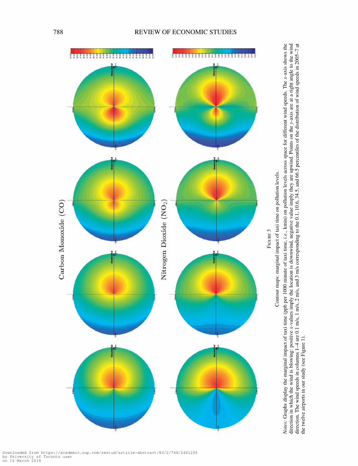
[17:34 10/3/2016 rdv043.tex] RESTUD: The Review of Economic Studies Page: 788 768–809
788 REVIEW OF ECONOMIC STUDIES
Figu
re3
Con
tour
map
s:m
argi
nali
mpa
ctof
taxi
time
onpo
llutio
nle
vels
.
Not
es:
Gra
phs
disp
lay
the
mar
gina
lim
pact
ofta
xitim
e(p
pbpe
r10
00m
inut
eof
taxi
time,
i.e.
,km
in)
onpo
llutio
nle
vels
acro
sssp
ace
for
diff
eren
twin
dsp
eeds
.The
x-ax
issh
ows
the
dire
ctio
nin
whi
chth
ew
ind
isbl
owin
g:po
sitiv
ex-
valu
esim
ply
the
loca
tion
isdo
wnw
ind,
nega
tive
valu
eim
ply
they
are
upw
ind.
Poin
tson
the
y-ax
isar
eat
ari
ght
angl
eto
the
win
ddi
rect
ion.
The
win
dsp
eeds
inco
lum
ns1–
4ar
e0.
1m
/s,1
m/s
,2m
/s,a
nd3
m/s
corr
espo
ndin
gto
the
0.1,
10.6
,34.
5,an
d66
.5pe
rcen
tiles
ofth
edi
stri
buti
onof
win
dsp
eeds
in20
05–7
atth
etw
elve
airp
orts
inou
rst
udy
(see
Figu
re1)
.
Downloaded from https://academic.oup.com/restud/article-abstract/83/2/768/2461206by University of Toronto useron 16 March 2018

[17:34 10/3/2016 rdv043.tex] RESTUD: The Review of Economic Studies Page: 789 768–809
SCHLENKER & WALKER AIRPORTS AND AIR POLLUTION 789
We use taxi time at three major airports in our baseline regressions: Atlanta (ATL), Chicago(ORD), and New York (JFK). Supplementary Table A7 presents first-stage F-statistics if weinstrument taxi time at California on up to four airports outside of California. Recall that weallow the coefficients to vary by airport, as network congestion will have different absoluteeffects on California airports. Irrespective of whether we use 1, 2, 3, or 4 airports outside ofCalifornia, the F-statistic is well above 10. In our baseline model, we use three airports that coverweather patterns in three regions of the Eastern US: Southeast (Atlanta), Midwest (Chicago),and Northeast (New York JFK), and the first-stage F-stat is 50. The fourth large airport outsideof California that we include in columns (d) is Dallas/Fort Worth (DFW). While results are notparticularly sensitive to including DFW, we exclude it from our baseline specifications as it issignificantly closer to California airports and thus may be more endogenous than the other threeairports (i.e. Dallas/Fort Worth may be delayed because California airports are delayed).
Reverse causality is less of a concern for the other three airports: a flight that leaves a Californiaairport at 6 am will not reach Atlanta, Chicago, or New York until roughly noon due to the changein time zones. Supplementary Table A8 tests for reverse causality directly by regressing taxi timeat an airport on eight weather measures we generally include as controls: a quadratic in minimumand maximum temperature, precipitation, as well as wind speed.37 The column heading givesthe airport at which the congestion is measured while the row indicates the airport at which theweather variables are measured.38 The table reports p-values of a hypothesis test pertaining tothe joint significance of the weather variables. The diagonal is highly significant as local weathermeasures impact airport taxi time. While weather at the eastern airports (ATL, ORD, or JFK)sometimes impacts taxi time at the two largest airports in California (LAX and SFO), the reverseis not true. This is consistent with weather at Eastern airports causing local network delays thatpropagate through the airspace and impact taxi time in California. The reverse direction does nothold. California airports do not affect East Coast airports on the same day. This result is not simplyan arteifact of there being less weather variation in California, as weather at LAX significantlyimpacts taxi time at SFO.
We have also run two sensitivity checks to further rule out endogeneity through reversecausality, the results of which are reported at the end of the subsequent section on health effectsand shown in Supplementary Table A13. First, we only utilize the combined taxi time between5 am and noon at the three major Eastern airports to rule out California feedback effects. Thisreduces the F-stat in model 1 from 50 to 35.5, but the results remain similar to baseline estimates.Second, instead of using taxi time at the three major Eastern airports, we use the eight weathervariables at each of these airports. Since this effectively increases the number of instrumentsby a factor of eight, we no longer estimate model 3 (which had 432 instruments to begin with).The F-statistic for the weather-instrumented regression is 5,436. Again, results remain similarto our baseline estimates but the standard errors in the second-stage increase. Going forward weinstrument using the overall daily taxi time, as it has a higher F-statistic than focusing only onthe mornings yet is more tractable than using weather measures, which would result in 3,456instruments in model 3.
We conduct two last robustness checks. First, since the variation in pollution due to delaysoutside of California should be uncorrelated with weather in California, we have estimated models(not reported) that exclude California weather controls altogether. Reassuringly, our baseline
37. Weather measures in our baseline regression also include the direction in which the wind is blowing relative tothe direction in which the zip code is located. Since the dependent variable in the current regression is at the airport leveland not the zip code level, these variables are not well defined and hence dropped.
38. If we pair airport taxi time with weather from another airport, we also include the local weather measure ascontrol. The local weather measures are not included in the joint test of significance.
Downloaded from https://academic.oup.com/restud/article-abstract/83/2/768/2461206by University of Toronto useron 16 March 2018

[17:34 10/3/2016 rdv043.tex] RESTUD: The Review of Economic Studies Page: 790 768–809
790 REVIEW OF ECONOMIC STUDIES
estimates for the most important pollutant (CO, see below) are similar whether we include orexclude California weather controls, but the error terms increase. Second, there may of coursebe some omitted variable that affects congestion outside of California and health outcomes inCalifornia. This hypothesis is not directly testable, but we have estimated models (available uponrequest) which include taxi time at other CA airports as a control variable in our baseline reducedform regressions, and the results remain very similar.
To put the magnitude of these effects into perspective, it is useful to consider the currentambient air standards in place for CO as regulated by the EPA under the Clean Air Act. Thecurrent one hour carbon monoxide standard specifies that pollution may not exceed 35 ppm (or35,000 ppb) more than once per year. California has their own CO standard which is 20 ppm. Aone standard deviation increase in LAX airplane idling (1,852 minutes) translates into an 83 ppbincrease (44.78×1.852) in carbon monoxide levels for areas within 10 km of LAX using estimatesfrom column (1a) of Table 1. Adding this number to the average daily maximum CO level at zipcodes from Panel A of Supplementary Table A2 (1234 ppb), the estimated increase in pollutionconcentrations is far below the current EPA standard. Similarly, for NO2, the current EPA 1-hourstandard is 100 ppb. Using estimates from column (2a) of Table 1, a standard deviation increasein LAX taxi time would lead to a 1 ppb increase in NO2 levels. Evaluated relative to the averagedaily maximum NO2 levels of 35.5 ppb, these are again well below the ambient criteria standard.Note that the maximum of the maximum daily NO2 levels is above the standard as some areasare out of attainment. The remaining sections estimate the social costs of these congestion-relatedincreases in ambient air concentrations by focusing on heath outcomes of the populations mostaffected by these emissions.
4.2. Effects of taxi time on local measures of health
We begin by investigating the “reduced form” health effects of airports, relating aggregate dailytaxi time to local measures of health. Namely, how does variation in airport congestion predictlocal health outcomes? Table 2 presents the results from a regression relating daily measures ofairport taxi time to local hospital admissions for the overall population as well as two susceptiblesubgroups: individuals below 5 years of age and individuals aged 65 years and above. Thedependent variable is measured as the daily sum of hospital and emergency room visits forpersons living in a particular zip code scaled by the population (per 10 million individuals) in thatparticular zip code. The regressions are weighted by zip code population size, and taxi time isinstrumented using taxi time at three major airports in the East. The estimated coefficient on thetaxi time variable corresponds to the increased rate of hospitalizations per 10 million individualsin a zip code for an extra 1,000 minutes of taxi time. Using various diagnosis codes, we examinethe impact of taxi time on asthma, respiratory, and heart-related admissions separately. As afalsification exercise, we also estimate the incidence of taxi time on strokes, bone fractures, andappendicitis rates. The reported standard errors are clustered on both zip code and day.
For the overall population (Panel A), all respiratory sickness rates as well as heart problemsare significantly impacted by taxi time, while the placebo effects for stroke, bone fractures, andappendicitis are not significantly affected. Results become larger in magnitude for the at-riskage groups. For the population 65 years and above, the incidence of stroke and bone fractures ismarginally significant at the 10% level. This may be do to statistical chance or may be explainedby the fact that senior citizens may also be more susceptible to sicknesses that covary withone another (e.g. a respiratory problem might make them fall and break a bone). Additionally,Medicare provides doctors implicit incentives to add additional diagnosis codes to receive higherreimbursement rates. Consistent with this explanation, models for which the dependent variable
Downloaded from https://academic.oup.com/restud/article-abstract/83/2/768/2461206by University of Toronto useron 16 March 2018

[17:34 10/3/2016 rdv043.tex] RESTUD: The Review of Economic Studies Page: 791 768–809
SCHLENKER & WALKER AIRPORTS AND AIR POLLUTION 791
TABLE 2Sickness rates regressed on instrumented taxi time
Acute All All Bone Appen-Asthma Respiratory Respiratory Heart Stroke fractures dicitis
(1a) (1b) (1c) (2) (3) (4) (5)
Panel A: all ages
Taxi Time 13.84∗∗∗ 24.77∗∗∗ 33.89∗∗∗ 19.35∗∗∗ 2.55 −1.33 0.26(2.72) (7.73) (9.82) (5.24) (1.71) (2.87) (0.68)
Panel B: ages below 5 years
Taxi Time 24.46∗∗ 84.28 116.12∗ 6.63∗ 0.80 2.16 −0.29(11.21) (51.35) (62.46) (3.47) (0.94) (5.84) (1.38)
Panel C: age 65 years and above
Taxi Time 36.89∗∗∗ 63.80∗∗∗ 100.53∗∗∗ 156.54∗∗∗ 22.87∗ 19.13∗ 0.75(11.39) (16.43) (25.25) (36.98) (12.95) (9.95) (1.21)
Observations 179,580 179,580 179,580 179,580 179,580 179,580 179,580Zip codes 164 164 164 164 164 164 164Days 1,095 1,095 1,095 1,095 1,095 1,095 1,095
Notes: Table regresses zip-code level sickness rates (counts for primary and secondary diagnosis codes per 10 millionpeople) on daily congestion (taxi time in 1000 min) that is caused by network delays (taxi time at three major airports in theEastern US). All regressions include weather controls (quadratic in minimum and maximum temperature, precipitationand wind speed as well as controls for wind direction), temporal controls (year, month, weekday, and holiday fixedeffects), and zip code fixed effects. Regressions are weighted by the total population in a zip code. Errors are two-wayclustered by zip code and day. Significance levels are indicated by ∗∗∗ 1%, ∗∗ 5%, ∗ 10%.
is measured only using the primary diagnosis code, the placebo effects for 65 years and older areno longer significant.
4.3. Hospital admissions and instrumented pollution exposure
Results thus far have shown that aggregate airplane taxi time generates variation in pollutionlevels of nearby communities. We exploit this variation to examine the relationship betweenpollution and health explicitly. Table 3 summarizes regression results for various pollutants andillnesses using a variety of traditional econometric specifications. Each entry corresponds to adifferent regression, where the dependent variable is measured as hospital admission rates, andthe independent variable is the daily mean ambient pollution concentration in a particular zipcode. As before, regression estimates are weighted by zip code population and standard errorsare clustered on both zip code and day.39
The first row within each panel presents estimates from a pooled OLS version of equation (5)without any controls Zzt , which suggests that increased ambient air concentrations lead toadverse health outcomes for respiratory and heart problems. Since various pollutants are oftencorrelated with one another, these estimates should be interpreted with caution, as the pollutant ofinterest will proxy for other correlated air pollutants. Each consecutive row adds more controls.The second row uses time controls (year, month, weekday, and holiday fixed effects), and thethird row additionally adds weather controls (quadratic in minimum and maximum temperature,precipitation and wind speed as well as controls for wind direction). To control for unobserved,
39. Unweighted regressions yield similar results and are available upon request.
Downloaded from https://academic.oup.com/restud/article-abstract/83/2/768/2461206by University of Toronto useron 16 March 2018

[17:34 10/3/2016 rdv043.tex] RESTUD: The Review of Economic Studies Page: 792 768–809
792 REVIEW OF ECONOMIC STUDIES
TABLE 3Sickness rates regressed on pollution
Acute All All Bone Appen-Asthma Respiratory Respiratory Heart Stroke fractures dicitis
(1a) (1b) (1c) (2) (3) (4) (5)
Panel A: CO pollution — all ages
No controls 0.070∗∗∗ 0.265∗∗∗ 0.353∗∗∗ 0.035 −0.002 −0.022∗∗∗−0.001(0.017) (0.041) (0.053) (0.028) (0.006) (0.007) (0.001)
Time controls 0.030 0.058 0.070 −0.022 −0.014∗ −0.008 0.001(0.024) (0.057) (0.075) (0.040) (0.008) (0.010) (0.001)
Time + Weather 0.056∗∗ 0.047 0.071 0.002 −0.005 −0.012 −0.001(0.028) (0.068) (0.091) (0.052) (0.010) (0.012) (0.001)
Time + Weather + Zip Code FE 0.011 0.049∗∗∗ 0.077∗∗∗ 0.027∗∗∗ −0.001 −0.007∗ 0.002(0.007) (0.018) (0.022) (0.008) (0.003) (0.004) (0.001)
Panel B: NO2 pollution — all ages
No controls 3.1∗∗∗ 10.7∗∗∗ 14.6∗∗∗ 4.3∗∗∗ 0.6∗∗∗ −0.3 0.1∗∗(0.5) (1.3) (1.7) (1.1) (0.2) (0.2) (0.0)
Time controls 1.7∗∗ 6.0∗∗∗ 7.9∗∗∗ 1.0 −0.1 0.6∗ 0.1∗∗(0.7) (1.5) (2.1) (1.4) (0.3) (0.3) (0.0)
Time + Weather 4.2∗∗∗ 8.3∗∗∗ 11.5∗∗∗ 3.0 0.8∗ 0.7 −0.0(1.0) (2.6) (3.6) (2.4) (0.5) (0.5) (0.1)
Time + Weather + Zip code FE 0.1 1.2∗ 2.5∗∗∗ 0.9∗∗∗ 0.1 −0.0 0.1∗(0.2) (0.6) (0.8) (0.3) (0.1) (0.2) (0.0)
Observations 179,580 179,580 179,580 179,580 179,580 179,580 179,580Zip codes 164 164 164 164 164 164 164Days 1,095 1,095 1,095 1,095 1,095 1,095 1,095
Notes: Table regresses zip code level sickness rates (based on primary and secondary diagnosis codes) on daily pollution(ppb) in 2005–7. Each entry is a separate regression. Columns use sickness rates (counts per 10 million people) fordifferent diseases, while rows use different controls. The first specification (row) in each panel has no controls, whilethe second adds time controls (year, month, weekday as well as holiday fixed effects), the third adds weather controls(quadratic in minimum and maximum temperature, precipitation and wind speed as well as controls for wind direction),and the fourth adds zip code fixed effects. All regressions are weighted by the total population in a zip code. Errors aretwo-way clustered by zip code and day. Significance levels are indicated by ∗∗∗ 1%, ∗∗ 5%, ∗ 10%.
time-invariant determinants of health, the fourth row of each panel in Table 3 reports regressionestimates from a model using zip code fixed effects. The model is identified by examining howwithin zip code changes in pollution are related to hospitalization rates of that particular zipcode. Again, pollution is often strongly correlated with health, although the estimates in thefourth row are usually smaller than those in the first three. These smaller point estimates areconsistent with time-invariant omitted variables introducing bias into the estimates from rowsone through three. Alternatively, classical measurement error in the pollution variable may leadto significant attenuation bias in fixed effects models (Griliches and Hausman, 1986), and thismay be responsible for the smaller point estimates in the last row.
Aside from attenuation bias, fixed effects models may also suffer from biases introducedby any unobserved, time-varying determinants of both pollution and health (e.g. weather). Toexplore this issue further, Table 4 presents instrumental variable estimates of the pollution–healthrelationship, using instrumented aggregate airport taxi time as an instrumental variable for dailymean pollution. Table 4 presents results for both the overall population in Panel A as well aschildren below 5 year in Panel B and people aged 65 years and above in Panel C.40 The three
40. Results for the two remaining groups: children ages 5–19 years and adults ages 19–64 years are given inSupplementary Table A9. Children between 5 and 19 years of age show no sensitivity to pollution shocks. Conversely,
Downloaded from https://academic.oup.com/restud/article-abstract/83/2/768/2461206by University of Toronto useron 16 March 2018

[17:34 10/3/2016 rdv043.tex] RESTUD: The Review of Economic Studies Page: 793 768–809
SCHLENKER & WALKER AIRPORTS AND AIR POLLUTION 793
TABLE 4Sickness rates regressed on instrumented pollution
Acute All Heart Bone Appen-Asthma respiratory respiratory problems Stroke fractures dicitis
(1a) (1b) (1c) (2) (3) (4) (5)
Panel A: all ages
Model 1: CO 0.311∗∗∗ 0.556∗∗∗ 0.761∗∗∗ 0.434∗∗∗ 0.057 −0.030 0.006(0.065) (0.162) (0.207) (0.134) (0.039) (0.063) (0.015)
Model 2: CO 0.307∗∗∗ 0.550∗∗∗ 0.755∗∗∗ 0.419∗∗∗ 0.050 −0.030 0.003(0.062) (0.163) (0.210) (0.128) (0.038) (0.064) (0.015)
Model 3: CO 0.194∗∗∗ 0.396∗∗∗ 0.515∗∗∗ 0.226∗∗∗ 0.020 −0.039 0.002(0.047) (0.125) (0.165) (0.079) (0.030) (0.040) (0.011)
Model 1: NO2 24.5∗∗∗ 43.8∗∗∗ 59.9∗∗∗ 34.2∗∗∗ 4.5 −2.4 0.5(6.2) (16.2) (20.5) (10.5) (3.1) (5.2) (1.2)
Model 2: NO2 24.3∗∗∗ 43.6∗∗∗ 59.8∗∗∗ 33.5∗∗∗ 4.2 −2.4 0.3(6.1) (16.3) (20.8) (10.4) (3.1) (5.2) (1.2)
Model 3: NO2 12.4∗∗∗ 18.9∗ 24.2∗ 17.1∗∗ 0.7 −1.0 0.3(4.0) (11.0) (14.2) (7.1) (2.2) (3.0) (0.9)
Panel B: ages below 5 years
Model 1: CO 0.565∗∗ 1.948∗ 2.683∗∗ 0.153∗ 0.018 0.050 −0.007(0.240) (1.124) (1.353) (0.081) (0.021) (0.136) (0.032)
Model 2: CO 0.579∗∗ 1.930∗ 2.624∗ 0.127 0.020 0.064 −0.013(0.235) (1.111) (1.356) (0.078) (0.023) (0.132) (0.034)
Model 3: CO 0.669∗∗∗ 2.166∗∗∗ 2.493∗∗ 0.075 0.023 −0.012 −0.009(0.170) (0.796) (0.980) (0.057) (0.015) (0.122) (0.022)
Model 1: NO2 42.2∗∗ 145.3 200.2∗ 11.4∗ 1.4 3.7 −0.5(20.5) (95.2) (117.3) (6.4) (1.6) (10.0) (2.4)
Model 2: NO2 43.2∗∗ 144.1 195.9∗ 9.5 1.5 4.8 −0.9(20.2) (94.3) (117.6) (6.2) (1.7) (9.7) (2.5)
Model 3: NO2 43.6∗∗∗ 122.2∗ 140.8∗ 4.5 2.9∗∗ 3.7 0.6(14.9) (67.7) (82.4) (4.6) (1.3) (9.3) (2.0)
Panel C: ages 65 years and older
Model 1: CO 0.849∗∗∗ 1.469∗∗∗ 2.314∗∗∗ 3.604∗∗∗ 0.526∗ 0.440∗ 0.017(0.312) (0.440) (0.642) (1.001) (0.297) (0.242) (0.028)
Model 2: CO 0.815∗∗∗ 1.413∗∗∗ 2.275∗∗∗ 3.529∗∗∗ 0.502∗ 0.409∗ 0.016(0.288) (0.422) (0.637) (0.971) (0.302) (0.241) (0.028)
Model 3: CO 0.493∗∗ 0.696∗∗ 1.424∗∗∗ 1.937∗∗∗ 0.198 0.187 −0.025(0.204) (0.309) (0.511) (0.620) (0.249) (0.161) (0.026)
Model 1: NO2 66.5∗∗∗ 114.9∗∗∗ 181.1∗∗∗ 282.0∗∗∗ 41.2∗ 34.5∗ 1.4(22.8) (34.3) (52.3) (76.1) (24.2) (18.2) (2.2)
Model 2: NO2 66.5∗∗∗ 115.1∗∗∗ 181.4∗∗∗ 282.2∗∗∗ 41.2∗ 34.5∗ 1.4(22.8) (34.3) (52.3) (76.2) (24.3) (18.2) (2.2)
Model 3: NO2 35.3∗∗ 38.9 75.8∗ 131.6∗∗∗ 3.6 12.2 −0.8(14.2) (24.6) (41.3) (47.8) (16.5) (12.0) (1.6)
Observations 179,580 179,580 179,580 179,580 179,580 179,580 179,580Zip codes 164 164 164 164 164 164 164Days 1095 1,095 1,095 1,095 1,095 1,095 1,095
Notes: Table regresses zip code level sickness rates (counts for primary and secondary diagnosis codes per 10 millionpeople) on daily instrumented pollution levels (ppb) in 2005–7. Each entry is a separate regression. Pollution isinstrumented on airport congestion (taxi time) that is caused by network delays (taxi time at three major airports inthe Eastern US). Model 1 assumes a uniform impact of congestion on pollution levels at all zip codes surrounding anairport, while model 2 adds an interaction with the distance to the airport, and model 3 furthermore adds interactions withwind direction and speed (columns (a)-(c) in Table 1). All regressions include weather controls (quadratic in minimumand maximum temperature, precipitation and wind speed as well as controls for wind direction), temporal controls (year,month, weekday, and holiday fixed effects), and zip code fixed effects. Regressions are weighted by the total populationin a zip code. Errors are two-way clustered by zip code and day. Significance levels are indicated by ∗∗∗ 1%, ∗∗ 5%,∗ 10%.
Downloaded from https://academic.oup.com/restud/article-abstract/83/2/768/2461206by University of Toronto useron 16 March 2018

[17:34 10/3/2016 rdv043.tex] RESTUD: The Review of Economic Studies Page: 794 768–809
794 REVIEW OF ECONOMIC STUDIES
rows (labeled model 1–3) use (1) taxi time, (2) taxi time interacted with distance, and (3) taxi timeinteracted with distance, wind speed, and wind direction, respectively. These are the specificationsoutlined in equations (1), (2), and (3) above.
The estimates in Table 4 are usually an order of magnitude larger than the OLS, fixed-effects estimates from Table 3. To put the magnitudes into perspective: the average asthmasickness rate for the overall population is 339 per 10 million inhabitants (Panel A1 and A2of Supplementary Table A3). The asthma coefficient for CO (model 3) in Table 4 implies that aone standard deviation increase in CO pollution leads to an additional 0.194×368=71 asthmaattacks per 10 million people,41 which is 21% of the daily mean.42 This suggests that fluctuationsin air pollution are a major cause of asthma related illnesses. For heart-related problems, therelative magnitude is 18% of the daily mean. It is important to note that the estimated CO effectmay not necessarily be coming from CO itself but from some other pollutant that is co-emittedin jet exhaust that we do not observe (e.g. a toxic VOC or particulate matter that is emitteddue to incomplete combustion). In addition to measurement error or avoidance behaviour, thefact that variation in CO comes from airplanes may be a further explanation for the discrepancybetween OLS and IV estimates. However, the Federal Aviation Administration (2005) suggeststhat aircraft engines produce the same types of emissions as automobiles, which are the largestsingle source of carbon monoxide emissions in the US.
Models 2 and 3 in Table 4 estimate over-identified models instrumenting pollution with bothtaxi time and taxi time interactions. While estimates in model 2 are similar to those from model 1,estimates from model 3 are generally smaller. The reason for the difference in magnitudes betweenmodels 2 and 3 is not entirely clear, but we believe there are two competing explanations. Thefirst explanation stems from the inability of models 1 and 2 to capture the spatial heterogeneity inthe effect of taxi time. Recall that model 3 uses distance as well as wind direction and wind speed.Marginal impacts of airport congestion vary greatly across space as shown in Figure 3, muchmore than in a model that only includes distance. Failing to model this heterogeneity in pollutionexposure may lead to inaccurate scaling of the reduced form relationships in our IV/2SLS setting.A competing explanation as to why model 3 estimates differ from models 1 and 2 stems frommeasurement error in the location of exposure. While we know the exact location of each pollutionmonitor and hence can correctly model the pollution surface in space, we only know the zip codeof a person’s residence and the hospital, not the exact location where they fell ill. As a result, allmodels will pair sickness counts with incorrect pollution measures if they are not close to thecentroid of the zip code when they fell ill, but this might be aggravated by model 3 that explicitlyuses the spatial distribution of the pollution surface. Supplementary Table A10 investigates thislatter hypothesis by looking at various subsets of the data. Panel A presents our baseline results,Panel B assigns pollution data based on the zip code of the residence, while Panel C assignspollution based on the hospital zip code. A few results are noteworthy: first, the estimates usingmodel specification 3 are very close to the estimates using specification 1 and 2 in Panel B1 wherewe only count sicknesses if both the zip code of the residence and hospital are within 10 km of thesame airport. On the other hand, model specification 3 diverges in Panel B2 where the hospitalzip code is outside the 10 km radius from airports, perhaps because we measure exposure less
the estimated dose–response for adults are roughly comparable to the baseline estimates, which is not surprising sincethey are the largest share of the overall population.
41. Panel A of Supplementary Table A2 shows that the standard deviation for CO is 368.42. This back-of-the-envelope calculation increases the pollution level in each zip code by the average ‘overall’
standard deviation of pollution fluctuations. Moreover, the average sickness rate is not population weighted. In subsequentsections, we increase pollution in each zip code by the zip code specific standard deviation in pollution fluctuations andcalculate the population-weighted average sickness count. The relative impact decreases to 17% of the daily mean underthe linear probability model and 19% under a Poisson count model.
Downloaded from https://academic.oup.com/restud/article-abstract/83/2/768/2461206by University of Toronto useron 16 March 2018

[17:34 10/3/2016 rdv043.tex] RESTUD: The Review of Economic Studies Page: 795 768–809
SCHLENKER & WALKER AIRPORTS AND AIR POLLUTION 795
accurately (e.g. the person might have been at work). In addition, panel B3 shows that there areno significant results where the hospital is within 10 km of another airport, suggesting that weare not simply picking up a daily pattern that is common to all airports.43 As a secondary bit ofevidence, model 3 in Panel B of our baseline Table 4 gives comparable point estimates to model1 and 2 for children under the age of 5 years, whom are more likely to be at home or in a close-byday care. Due to these competing explanations for the differences across models, we continueto present all model estimates whenever possible, allowing the reader to choose their preferredestimate.
There are two additional explanations for the discrepancies between models 3 and 1 and 2which we find less salient. First, there is a well-known bias of 2SLS estimators when instrumentsare weak and when there are many over-identifying restrictions (Bound et al., 1995). In linearmodels with iid errors, Stock et al. (2002) propose rule-of-thumb thresholds for F-statistics forthe first stage. However, in both the non-iid case (i.e. with clustered standard errors) and in caseswith multiple endogenous variables, less is known about the relationship between the F-statisticand the properties of instrumental variables estimates. Baum et al. (2003) suggest comparing thetest statistic to the Stock et al. (2002) critical values for the Cragg–Donald F statistic with a singleinstrument. According to this metric, results from Table 1 suggest that model 3 is a strong first-stage predictor of local pollution levels with a F-statistic that is 14 for CO pollution and to a lesserextent for NO2 pollution (F-stat of 5). The first stage in model 3 is not as strong as in models 1 and2, and the model is highly over-identified with twelve excluded instruments. Bound et al. (1995)show how the bias of 2SLS increases in the number of instruments and decreases in the strengthof the first stage. The bias of 2SLS in the case of weakly identified or over-identified models istowards the OLS counterpart. Since this is consistent with model 3 estimates in Table 4 beingsmaller than both model 1 and 2 but still above the OLS estimates, Supplementary Table A11estimates models 2 and 3 using Limited Information Maximum Likelihood (LIML), which ismedian-unbiased for over-identified, constant-effects models (Davidson and MacKinnon, 1993).Results remain similar, which suggests that weak instrument attenuation is less of a concern(Angrist and Pischke, 2008). Finally, a second alternative explanation for why model 3 giveslower point estimates is that the hourly wind data represent snapshots of the wind speed anddirection and include significant measurement error. However, this is somewhat at odds with thefact that we find such significant spatial patterns in the pollution regressions.
Panels B and C of Table 4 present estimates for children and senior citizens. While the dose–response relationships are larger, so are average sickness rates. In relative terms, a one standarddeviation increase in CO pollution now causes a 37% increase in asthma cases for children under5 years compared to the average daily mean. On the other hand, a one standard deviation increasein CO pollution causes a 24% increase in heart problems for people 65 years and above. The higher‘absolute’ sensitivity in Panel B and C suggests that there may exist significant heterogeneity inthe population response to ambient air pollution exposure. Since the population aged 65 yearsand older has guaranteed access to health insurance through Medicare, they may be more inclinedto visit the emergency room or hospital relative to the rest of the population, leading to largerestimated effects. On the other hand, the relative magnitude compared to average sickness ratesare only slightly larger than for the overall population.
Columns (3)–(5) of each panel includes results for one of three placebos: strokes, bonefractures, and appendicitis. Both strokes and appendicitis are severe enough that people should goto the hospital. None of the results are significant for the overall population in Panel A. Consistentwith the reduced form evidence in Table 2, some of the coefficients in Panel C are significant
43. If we assign pollution based on the hospital zip code in panels C, results are generally not significant.
Downloaded from https://academic.oup.com/restud/article-abstract/83/2/768/2461206by University of Toronto useron 16 March 2018

[17:34 10/3/2016 rdv043.tex] RESTUD: The Review of Economic Studies Page: 796 768–809
796 REVIEW OF ECONOMIC STUDIES
at the 10% level. In Supplementary Table A12 we replicate the analysis using only the primarydiagnosis code. None of the placebo regressions remain significant. Since we are interested in theoverall effect of pollution on hospitalization rates, our baseline models continue to count totalsickness counts for both primary and secondary diagnoses.
Supplementary Table A13 further investigates the sensitivity of our IV estimates to differentchoices of instrumental variables.As a point of comparison, PanelAreplicates the baseline resultsof Table 4 for all ages. Panel B instruments for pollution using only the taxi time between 5 amand noon at Eastern airports to rule out endogeneity through reverse causality. The results remainrobust to this change. Panel C goes one step further and instruments for taxi time at Californiaairports using only weather measures at the three major airports in the Eastern US. While thepoint estimates remain comparable, the standard errors generally increase.44
4.3.1. Jointly estimating the effect of ambient air pollutants. A common challenge instudies linking health outcomes to pollution measures is that ambient air pollutants are highlycorrelated. It is therefore difficult to determine empirically which pollutant is the true causeof any observed changes in health. Our research design provides one possible solution to theidentification problem. Wind speed and wind direction differentially affect both CO and NO2dispersion patterns. Moreover, the rate of CO and NO2 emissions depend on the thrust producedby the engine, and higher wind speeds require more engine thrust. Wind speed hence impacts boththe rate at which pollutants are produced and how they disperse. Table 5 estimates the joint effectof both CO and NO2 on health using our first stage model with wind speed and wind directioninteractions (model 3).
In all specifications for which we have multiple endogenous variables, we report theAngrist and Pischke (2008) conditional F-statistics in the tables and text, although these aresomewhat hard to interpret. As mentioned above, there are no rule-of-thumb thresholds for linearmodels with non-iid errors or for models with multiple endogenous variables. When comparingthe conditional F-statistics to the Stock et al. (2002), the F-statistics suggest that the first stageis “weak”. Perhaps more usefully, in all specifications for which we have multiple endogenousvariables, we also present two tests that are robust to issues pertaining to weak instruments,the Anderson–Rubin test statistic and the closely related Stock-Wright (2000) S statistic. Thenull hypothesis tested in both cases is that the coefficients of the endogenous regressors in thestructural equation are jointly equal to zero, and, in addition, that the overidentifying restrictionsare valid. We use a cluster-robust version of both test statistics that has the correct size even underweak identification (Chernozhukov and Hansen, 2008). The tests are equivalent to estimating thereduced form of the equation (with the full set of instruments as regressors) and testing that thecoefficients of the excluded instruments are jointly equal to zero. In most specifications, inferencebased on the Anderson–Rubin and Stock–Wright tests are consistent with inference based on theWald test of the same null hypothesis. This suggests that we are not drawing spurious inferencesbased on weak instruments. We also present results using LIML because LIML is approximatelymedian unbiased for overidentified models, and the results are similar between 2SLS and LIML.When 2SLS is subject to weak instrument bias, the 2SLS estimand will diverge significantly fromthe LIML estimand toward the OLS estimand. Thus, the fact that LIML and 2SLS deliver similarresults assuages our concerns pertaining to significant biases associated with weak instruments.45
Table 5 shows that the coefficient for CO remains comparable in size to our baselineestimates from Table 4, albeit slightly larger. Conversely, the coefficients on NO2 switch
44. We do not estimate model 3 using weather variables as it would include 3,456 instruments.45. A similar diagnostic exercise of this nature can be found on pages p. 213–215 of Angrist and Pischke (2008).
Downloaded from https://academic.oup.com/restud/article-abstract/83/2/768/2461206by University of Toronto useron 16 March 2018

[17:34 10/3/2016 rdv043.tex] RESTUD: The Review of Economic Studies Page: 797 768–809
SCHLENKER & WALKER AIRPORTS AND AIR POLLUTION 797
TABLE 5Sickness rates regressed on instrumented pollution — joint estimation
Acute All Heart Bone Appen-Asthma respiratory respiratory problems Stroke fractures dicitis
(1a) (1b) (1c) (2) (3) (4) (5)
Panel A: All Ages
Model 3: CO 0.222∗∗ 0.867∗∗∗ 1.189∗∗ 0.105 0.054 −0.127∗ −0.006(0.106) (0.313) (0.476) (0.139) (0.049) (0.073) (0.017)
Model 3: NO2 −2.2 −40.1 −57.4 10.7 −2.9 7.6 0.7(8.0) (25.6) (38.4) (13.4) (3.5) (5.6) (1.5)
F(1st stage) - CO 4.18 4.18 4.18 4.18 4.18 4.18 4.18F(1st stage) - NO2 1.57 1.57 1.57 1.57 1.57 1.57 1.57P(Anderson-Rubin) 0.0000 0.0000 0.0000 0.0012 0.0027 0.1418 0.0484P(Stock-Wright S) 0.0413 0.0795 0.1141 0.1232 0.5319 0.4795 0.5710
Panel B: ages below 5 years
Model 3: CO 0.901 4.685∗∗ 5.388∗∗ 0.133 −0.073 −0.385 −0.102(0.599) (2.167) (2.483) (0.142) (0.051) (0.355) (0.072)
Model 3: NO2 −18.8 −206.8 −237.6 −4.8 8.0∗ 30.9 7.7(46.1) (174.9) (199.0) (11.5) (4.1) (27.3) (6.4)
F(1st stage) - CO 3.39 3.39 3.39 3.39 3.39 3.39 3.39F(1st stage) - NO2 1.30 1.30 1.30 1.30 1.30 1.30 1.30P(Anderson-Rubin) 0.0000 0.0001 0.0000 0.0185 0.0474 0.0687 0.6100P(Stock-Wright S) 0.0588 0.0886 0.2163 0.4046 0.3567 0.3185 0.5764
Panel C: age 65 years and above
Model 3: CO 0.268 0.775∗ 1.726∗∗ 1.279 0.490 0.147 −0.051(0.323) (0.445) (0.772) (0.821) (0.399) (0.281) (0.046)
Model 3: NO2 20.1 −6.4 −25.8 60.3 −25.5 3.7 2.2(22.1) (36.3) (62.6) (67.7) (25.9) (21.4) (3.1)
F(1st stage) - CO 4.96 4.96 4.96 4.96 4.96 4.96 4.96F(1st stage) - NO2 2.09 2.09 2.09 2.09 2.09 2.09 2.09P(Anderson-Rubin) 0.1146 0.0026 0.0035 0.0009 0.0164 0.1595 0.0017P(Stock-Wright S) 0.4530 0.1484 0.2756 0.1831 0.3849 0.2969 0.1264
Observations 179,580 179,580 179,580 179,580 179,580 179,580 179,580Zip codes 164 164 164 164 164 164 164Days 1,095 1,095 1,095 1,095 1,095 1,095 1,095
Notes: Table regresses zip code level sickness rates (counts for primary and secondary diagnosis codes per 10 millionpeople) on daily instrumented pollution levels (ppb) in 2005–7. The effect of the two pollutants is jointly estimated forthe over-identified model 3 using LIML. Pollution is instrumented on airport congestion (taxi time) that is caused bynetwork delays (taxi time at three major airports in the Eastern US). All regressions include weather controls (quadraticin minimum and maximum temperature, precipitation and wind speed as well as controls for wind direction), temporalcontrols (year, month, weekday, and holiday fixed effects), and zip code fixed effects. Regressions are weighted by thetotal population in a zip code. Errors are two-way clustered by zip code and day. Significance levels are indicated by∗∗∗ 1%, ∗∗ 5%, ∗ 10%.
sign and are mostly negative and insignificant. We have also used the methods proposed byChernozhukov and Hansen (2008) to build non-spherical confidence regions for the multipleendogenous variables. Within the joint parameter space of CO and NO2, the joint confidenceregion lies in the quadrant where CO is positive and NO2 is weakly negative.46
46. The full set of results, which consist of two- dimensional plots for each hypothesis test, are available uponrequest.
Downloaded from https://academic.oup.com/restud/article-abstract/83/2/768/2461206by University of Toronto useron 16 March 2018

[17:34 10/3/2016 rdv043.tex] RESTUD: The Review of Economic Studies Page: 798 768–809
798 REVIEW OF ECONOMIC STUDIES
We interpret these findings as evidence that the returns from regulating CO exceed those fromregulating NO2, at least for the population that comprises our sample. One possible explanationfor our results stems from the work done by Auffhammer and Kellogg (2011). Figure 9 ofAuffhammer and Kellogg (2011) shows that the Southern California coastline, the location ofmost of the zip codes in our study, ozone generation seems VOC limited, i.e., a reduction in VOCreduces ozone. Conversely, regions further inland and in Northern California are NO2 limited.Reducing NO2 in areas that are VOC limited has little effect on ozone, and this may be the reasonwe observe small and insignificant results for NO2. In the remainder of the article, we thereforefocus on CO.
4.3.2. Threshold effects and non-linearities in the pollution-health relationship.We explore the functional form of the dose-response function in four separate ways.First, Supplementary Table A14 estimates the relationship separately for the summer (April–September) and the winter (October–March). Each panel of the table provides the point estimatesfor the two seasons from a joint regression where all variables and instruments are interactedwith seasonal dummies as well as the p-values of a test whether the coefficients are the same.Especially for the case of children under the age of 5 years, the effect seem to be significantlyhigher during winter months when average pollution levels are higher.
Recall that CO and NO2 pollution are higher during the winter months, so a non-lineardose–response function that has increasing marginal damages of pollution should exhibit largercoefficients for the winter months. The coefficient for the winter months is almost always largerthan for the summer months for the illnesses that are related to pollution (columns (1a)–(2)). Theseresults are consistent with increasing marginal impacts of pollution. However, there may be otherimportant differences in health outcomes across seasons that could explain these disparities. Anobvious candidate for differences between the summer and the winter would be the level ofambient ozone concentrations which tend to be much higher in the summer than the winter. Inadditional results (Supplementary Table A15), we control for ozone levels as a potential confoundand the results are nearly identical. One possible explanation for why ozone does not impact thebaseline regression results stems from measurement error in the excluded ozone regressor and/oravoidance behaviour pertaining to ozone.
We have also explored models which estimate the possible non-linear effects of pollution onhealth outcomes by including higher order polynomials. Models with higher-order pollution termsincrease the number of endogenous variables in our regressions, and we use the overidentifiedmodel 3 to instrument for the higher order terms. Since higher-order polynomials can be difficult tointerpret, Supplementary Figure A5 plots the predicted marginal effects of the pollutant on a rangeof health outcomes as a function of the ‘level’of the pollutant on the given day. That is, we plot thedose response function, where the y-axis measures the health response and the x-axis measuresthe level of pollution. Since we are fitting non-linear models, the responsiveness is allowed to varyacross the x-axis. The dashed line displays the results from our baseline, linear dose–responsemodel (constant marginal damage). The solid represents results from a quadratic model wherethe 95% confidence interval is added in grey. The four columns represent the four sicknessesthat are related to pollution fluctuations (asthma, acute respiratory, all respiratory, and heartproblems, respectively). The predicted marginal effect is plotted over the empirical distributionof daily pollution levels, from the 5th to the 95th percentile.47 While there is some evidence thatrespiratory problems (columns 1–3) exhibit increasing marginal damages as pollution levels startto increase, again especially for children under the age of 5 years, the confidence intervals reflect
47. Supplementary Figure A4 shows the observed distribution of daily CO levels in our data set.
Downloaded from https://academic.oup.com/restud/article-abstract/83/2/768/2461206by University of Toronto useron 16 March 2018

[17:34 10/3/2016 rdv043.tex] RESTUD: The Review of Economic Studies Page: 799 768–809
SCHLENKER & WALKER AIRPORTS AND AIR POLLUTION 799
an inability to reject the null that the damage function is constant over the observed range of COvalues.
We have investigated non-linearities in two additional ways that are broadly consistent with thefindings above (results available upon request). First, we estimated models whereby we interactedour daily pollution variation of interest with the mean pollution ‘level’ in a zip code. This allowsthe dose–response curve to vary (linearly) in the level of average pollution levels of a zip code.If this interaction term is zero, this would support the hypothesis that the marginal effect of aone unit increase in emissions is the same regardless of the level of ambient air pollution (i.e.a constant, linear dose–response). If the coefficient on the interaction was significantly positive,then this would support the hypothesis that the marginal effect of ambient air pollution on healthoutcomes is progressively worse in areas with higher than average pollution levels. A challengewith this particular test is that the average level of ambient air pollution in a zip code can becorrelated with many observed and unobserved factors that may contribute to heterogeneity in thedose-response relationship. For example, people in more polluted areas may lack basic preventivehealth services and thus be ‘more’ responsive to marginal changes in air pollution because of theirunderlying health conditions rather than any non-linearity in the dose–response. Nevertheless,results suggest (available upon request) that CO exhibits an increasing dose-response function.Second, we explored the shape of the dose-response function in an OLS, fixed effects setting.While we think the regression coefficient ‘magnitudes’ may be attenuated by things such asmeasurement error and/or avoidance type behaviours, the ‘shape’ of the dose-response curve islikely less sensitive to these concerns (unless of course the bias varied with the level of pollution— which might happen through avoidance behaviour such as “bad air day” alerts). We use thislogic to explore the shape of the dose-response function by fitting OLS, fixed-effect regressionmodels that include polynomials in the daily mean pollution level (i.e. quadratic, cubic, or quartic).We then plot the predicted marginal effects of the pollutant on a range of health outcomes as afunction of the ‘level’ of the pollutant on the given day (as in Supplementary Figure A5). We seethat for both asthma and respiratory illness, the predicted marginal effect is increasing in the levelof the pollutant. The patterns suggests some sort of “threshold” by which the marginal effect ofCO on health outcomes “flattens out”.
While the various results in this section come from different econometric models, theconclusions pertaining to the shape of the dose-response function remain similar across thespecifications. The evidence suggests that the marginal effect of pollution is increasing in the levelof the pollutant, but at a decreasing rate. The diminishing marginal damages of the dose-responsefunction is also consistent with modern evidence from epidemiology (see e.g. Pope et al. (2009)and Pope III et al. (2011)).
4.3.3. Potential confounding sources of variation. While our estimates suggest thatCO is primarily responsible for the observed health responses, there may be other sources ofunobserved, concomitant variation that may lead to similar relationships. For example, whilewe estimate the effect of CO and NO2 in the same model, we do not directly control for otherpollutants such as ozone. It seems unlikely that ozone O3 is causing the observed relationship. Asmentioned above, Supplementary Table A14 estimates the relationship separately for the summer(April–September) and the winter (October–March). Ozone is higher during the summer, whileCO and NO2 are higher during the winter. The observed health effects are larger and moresignificant during the winter time when ozone is not a big problem. We have also estimatedmodels that directly control for ozone (Supplementary Table A15), and the results remain similarand a bit more precise than our baseline estimates. The standard errors are also much larger forthe summer, especially in the case of acute respiratory problems and overall respiratory problems.
Downloaded from https://academic.oup.com/restud/article-abstract/83/2/768/2461206by University of Toronto useron 16 March 2018

[17:34 10/3/2016 rdv043.tex] RESTUD: The Review of Economic Studies Page: 800 768–809
800 REVIEW OF ECONOMIC STUDIES
This is not surprising, because other pollutants like ozone also impact health outcomes, whichwill be part of the error term.
One potential omitted variable that we unfortunately cannot measure well is particulatematter, a pollutant which may emerge from combustion emissions and has been shown in thepast to increase infant mortality due to respiratory causes (Currie and Neidell, 2005). Particulatematter monitors in California are limited in both their spatial and temporal coverage; readings onambient particulate monitors are conducted every few days (as opposed to hourly data from otherpollutants), and there are far fewer monitors. These limitations do not square well with our researchdesign which relies on high-frequency, daily variation across very localized areas. Nevertheless,we have directly explored the degree to which particular matter predicts adverse health outcomesfor the subsample of days and locations for which we have particulate monitor data. Table A16presents results using the full set of particulate monitors for PM2.5.48 Supplementary Table A16suggests that PM does not have much explanatory power in predicting health outcomes, althoughthe standard errors preclude definitive conclusions.49 Recall that Los Angeles Airport is not asignificant point source of particulate matter. While it is the largest point source for CO emissionsin the state of California, it only ranks 2,763 and 2,782 among emissions of PM10 and PM2.5.Even still, we believe that some amount of caution is warranted in interpreting CO as the uniquepollutant-related causal channel leading to adverse health outcomes; there may be in fact otherunobserved sources of ambient air pollution that covary with CO that may also affect health.
4.3.4. Inpatient versus outpatient data. Traditionally, studies have relied on Inpatientdata sets to examine health responsiveness to various external factors such as pollution. Onelimitation of such data is that a person only enters the Inpatient data set if they are admittedfor an overnight stay in the hospital. Many ER visits result in a discharge the same day andhence never result in an overnight stay. Starting in 2005, California began collecting Outpatient(Emergency Room) data. Previous published estimates all replied on Inpatient data only. To betterunderstand the differences between these two datasets as well as compare our results to those fromthe previous literature, we replicate the analysis using sickness counts from only the Inpatientdata in Panels A1–C1 in Supplementary Table A17. By the same token, Panels A2–C2 only usesthe Outpatient data.50 Not surprisingly, there is a significant relationship between pollution andheart problems (column 2) in the Inpatient data for patient ages 65 years and above (as theseconditions usually require an overnight stay), but no or very limited sensitivity of asthma oroverall respiratory illnesses (columns 1a and 1c) to pollution. Conversely, the Outpatient (ER)data shows a much larger sensitivity of respiratory problems to changes in pollution. These resultsshow the importance of Outpatient (ER) data when studying the morbidity effects of ambient airpollution on health outcomes.
4.3.5. Temporal displacement and dynamics. Our baseline regression models examineonly the contemporaneous effect of pollution on health. Contemporaneous estimates may lead tounderestimates of the total effects of air pollution on health if health effects respond sluggishlyto changes in pollution. Conversely, estimates may overstate the hypothesized effect due to
48. Unfortunately, we only observe 2 PM10 pollution monitors within 15 km of an airport (or equivalently two- zipcodes) which makes our research design infeasible due to the importance of distance and wind angle/speed heterogeneity.
49. All of the estimates in Supplementary Table A16 come from limited information maximum likelihood estimatesas opposed to 2SLS (although results are similar).
50. Patients that enter the ER and are later admitted for an overnight stay are dropped from the ER data to avoiddouble counting.
Downloaded from https://academic.oup.com/restud/article-abstract/83/2/768/2461206by University of Toronto useron 16 March 2018

[17:34 10/3/2016 rdv043.tex] RESTUD: The Review of Economic Studies Page: 801 768–809
SCHLENKER & WALKER AIRPORTS AND AIR POLLUTION 801
temporal displacement: if spikes in daily pollution levels make already sick people go to thehospital one day earlier, contemporaneous models overestimate the true effect associated withpermanently higher pollution levels. If temporal displacement is important, the contemporaneousincrease in sickness rates should be followed by a decrease in sickness rates in subsequentperiods.
We investigate both of these issues by estimating a distributed lag regression model, includingthree lags in the pollution variable of interest. Table 6 presents the distributed lag results ofpollution for the overall population. We present individual coefficients as well as the combinedeffect (the sum of the four) in the last row of each panel. To preserve space, we only list theresults for the sickness categories that are impacted by changing CO pollution levels. Sinceregulatory policy is concerned with the health effects of a permanent change in pollution, wefocus on cumulative effects of the model over the estimated 4 day horizon. The cumulative effectis slightly larger than the comparable baseline results in Table 4. This might be because someindividuals delay hospital visits, although the exact dynamics are hard to determine empiricallygiven the lack of significance of the individual coefficients. We have also experimented withdifferent leads/lags (available upon request). For example, in a model with three leads and sixlags, the sum of the six lags and contemporaneous terms are similar in magnitude. The threeleads, on the other hand, are not jointly significant.
4.3.6. Count model. Our baseline health estimates consist of linear probability models,relating the population-scaled hospital admission rates to changes in pollution. To account for thenon-negative and discrete nature of the hospital admission data, Table 7 presents estimates froma quasi-maximum likelihood, conditional Poisson IV estimator given in equation (8). In contrastto the baseline linear probability health models, these models are not weighted. In addition,since we use a control function to address issues pertaining to measurement error and omittedvariables, we adjust standard errors for the first stage sampling variation using a block-bootstrapsampling procedure, resampling zip codes.51 Analogous to the linear probability model, we findthat respiratory illnesses and heart problems are sensitive to pollution fluctuations, while the threeplacebos are not (with the usual caveat applying to sickness counts for people aged 65 years andabove).
The coefficients no longer give marginal impacts and are difficult to interpret. In order tocompare the marginal impacts of pollution exposure and congestion across all of our models,Table 8 presents the predicted increase in sickness counts from (1) a one standard deviationincrease in taxi time, and (2) a one standard deviation increase in pollution levels in each zipcode. The results are then added for all zip codes that are within 10 km of an airport. The tablealso summarizes population surrounding airports. Various admission categories are given in rows,while the columns show the results for each of the twelve airports. The last column gives thecombined impact among all twelve airports.
Panels A, B, and C give the predicted increase in hospital admissions using estimates fromthe baseline linear probability model whereby pollution is instrumented using model 3 (pollutioninstrumented with taxi time + interactions with distance and wind direction). These results arepresented for the overall population (PanelA), children below 5 years (Panel B), and senior citizens65 years and above (Panel C). Panel D gives the results for the overall population using the countmodel shown in Table 7. Impacts are evaluated at the sample mean for the nonlinear Poissonmodel. The results from the Poisson model are similar to those from the linear probability model
51. This is equivalent to clustering by zip code instead of two-way clustering by zip code and day. An unweightedregression of the linear probability model (available upon request) that clusters by zip code gives comparable results.
Downloaded from https://academic.oup.com/restud/article-abstract/83/2/768/2461206by University of Toronto useron 16 March 2018

[17:34 10/3/2016 rdv043.tex] RESTUD: The Review of Economic Studies Page: 802 768–809
802 REVIEW OF ECONOMIC STUDIES
TABLE 6Sickness rates of all ages regressed on instrumented CO pollution — lagged pollution
Acute All HeartAsthma respiratory respiratory problems
Model 1
Pollution in t-3 0.026 0.220 0.345 0.022(0.096) (0.188) (0.250) (0.139)
Pollution in t-2 0.130 0.109 0.023 0.003(0.143) (0.246) (0.336) (0.255)
Pollution in t-1 −0.017 −0.060 −0.001 −0.020(0.132) (0.251) (0.289) (0.183)
Pollution in t 0.200∗∗ 0.355 0.485 0.422∗∗∗(0.101) (0.263) (0.331) (0.134)
Cum. Effect 0.339∗∗∗ 0.624∗∗∗ 0.853∗∗∗ 0.427∗∗∗(0.070) (0.163) (0.210) (0.151)
Model 2
Pollution in t-3 0.040 0.229 0.353 0.022(0.094) (0.188) (0.250) (0.138)
Pollution in t-2 0.117 0.098 0.013 −0.002(0.141) (0.245) (0.331) (0.250)
Pollution in t-1 −0.021 −0.062 −0.004 −0.028(0.133) (0.253) (0.291) (0.184)
Pollution in t 0.203∗∗ 0.352 0.485 0.415∗∗∗(0.099) (0.262) (0.331) (0.132)
Cum. Effect 0.338∗∗∗ 0.618∗∗∗ 0.847∗∗∗ 0.408∗∗∗(0.066) (0.163) (0.214) (0.143)
Model 3
Pollution in t-3 −0.002 0.126 0.121 0.045(0.041) (0.095) (0.124) (0.057)
Pollution in t-2 0.079 0.023 0.020 −0.014(0.060) (0.116) (0.151) (0.087)
Pollution in t-1 −0.059 0.008 0.020 −0.004(0.056) (0.154) (0.191) (0.111)
Pollution in t 0.177∗∗∗ 0.316 0.420 0.225∗∗(0.067) (0.201) (0.263) (0.100)
Cum. Effect 0.195∗∗∗ 0.473∗∗∗ 0.582∗∗∗ 0.252∗∗∗(0.052) (0.115) (0.153) (0.067)
Observations 179,088 179,088 179,088 179,088Zip Codes 164 164 164 164Days 1,092 1,092 1,092 1,092
Notes: Table replicates the results of CO pollution on sickness counts for all ages in Table 4 except that three lags of theinstrumented pollution levels are included. Each column in each panel presents the coefficients from one regression aswell as the cumulative effect (sum of all four coefficients). Significance levels are indicated by ∗∗∗ 1%, ∗∗ 5%, ∗ 10%.
in Panel A. Panel E gives the average daily sickness count in 2005–7 for the overall populationfor comparison.
Pollution fluctuations have a large effect on the 6 million people living within 10 km of one ofthe twelve airports:Aone standard deviation increase in a zip-codes specific pollution fluctuationsincreases asthma counts for the overall population by 17% under the linear probability model
Downloaded from https://academic.oup.com/restud/article-abstract/83/2/768/2461206by University of Toronto useron 16 March 2018

[17:34 10/3/2016 rdv043.tex] RESTUD: The Review of Economic Studies Page: 803 768–809
SCHLENKER & WALKER AIRPORTS AND AIR POLLUTION 803
TABLE 7Sickness counts regressed on instrumented CO pollution — poisson model
Acute All Heart Bone Appen-Asthma respiratory respiratory problems Stroke fractures dicitis
(1a) (1b) (1c) (2) (3) (4) (5)
Panel A: all ages
Model 1: CO 0.834∗∗∗ 0.596∗∗∗ 0.577∗∗∗ 0.488∗∗∗ 0.270 −0.114 0.325(0.171) (0.109) (0.112) (0.128) (0.184) (0.184) (0.454)
Model 2: CO 0.846∗∗∗ 0.589∗∗∗ 0.573∗∗∗ 0.482∗∗∗ 0.246 −0.116 0.245(0.172) (0.111) (0.116) (0.128) (0.185) (0.188) (0.466)
Model 3: CO 0.561∗∗∗ 0.399∗∗∗ 0.378∗∗∗ 0.292∗∗∗ 0.132 −0.150 0.163(0.132) (0.090) (0.087) (0.095) (0.195) (0.133) (0.325)
Panel B: ages below 5 years
Model 1: CO 1.202∗∗∗ 0.237 0.303 2.061∗ 3.334 0.187 −0.369(0.387) (0.179) (0.208) (1.148) (2.876) (0.572) (2.923)
Model 2: CO 1.202∗∗∗ 0.216 0.278 1.891∗ 3.347 0.233 −0.691(0.396) (0.179) (0.207) (1.105) (2.799) (0.567) (2.963)
Model 3: CO 1.133∗∗∗ 0.261∗∗ 0.256∗ 1.297 4.238∗ −0.064 −1.290(0.287) (0.132) (0.143) (0.966) (2.480) (0.495) (2.643)
Panel C: ages 65 years and older
Model 1: CO 1.287∗∗∗ 0.757∗∗∗ 0.610∗∗∗ 0.634∗∗∗ 0.397∗ 0.626∗∗ 1.190(0.364) (0.208) (0.173) (0.165) (0.219) (0.314) (1.247)
Model 2: CO 1.264∗∗∗ 0.743∗∗∗ 0.608∗∗∗ 0.630∗∗∗ 0.388∗ 0.589∗ 1.135(0.341) (0.202) (0.174) (0.166) (0.224) (0.313) (1.291)
Model 3: CO 0.804∗∗∗ 0.413∗∗ 0.397∗∗ 0.369∗∗∗ 0.159 0.292 −0.852(0.275) (0.180) (0.154) (0.126) (0.223) (0.219) (1.185)
Observations 179,580 179,580 179,580 179,580 179,580 179,580 179,580Zip Codes 164 164 164 164 164 164 164Days 1,095 1,095 1,095 1,095 1,095 1,095 1,095
Notes: Table replicates the results for regression models of CO in Table 4 except that we use a Poisson count modelinstead of a linear probability model. Further differences are that the regressions are unweighted and standard errors areobtained from 100 clustered bootstrap draws (drawing entire zip code histories with replacement), which is comparableto clustering by zip code in the baseline regression. Significance levels are indicated by ∗∗∗ 1%, ∗∗ 5%, ∗ 10%.
and 19% under the Poisson count model.52 Overall, a one standard deviation increase in zip codespecific ‘daily’ pollution levels results in 107 additional admissions for respiratory problemsand 49 additional admissions for heart problems, which are 17% and 9% of the daily mean.For respiratory problems, infants only account for roughly one third of the overall impacts.Studies focusing only on the impact on infants therefore would miss a significant portion of theoverall impacts. Not surprisingly, the elderly are responsible for the largest share of heart relatedimpacts.
Airport congestion significantly contributes to the overall impacts: a one standard deviationincrease in taxi time increases respiratory and heart admissions by roughly 1% of the dailymean. At LAX, the largest airport in California, a one standard deviation increase in taxi time isresponsible for roughly one-fourth of the effect of a one-standard deviation increase in pollution.
52. Recall that these estimates are smaller than what we reported under Table 4, where we increased pollution levelsin each zip code by the average ‘overall’ standard deviation in pollution levels and took an average baseline sickness ratethat was not population weighted.
Downloaded from https://academic.oup.com/restud/article-abstract/83/2/768/2461206by University of Toronto useron 16 March 2018

[17:34 10/3/2016 rdv043.tex] RESTUD: The Review of Economic Studies Page: 804 768–809
804 REVIEW OF ECONOMIC STUDIES
TABLE 8Impact of CO pollution on health (Model 3)
LAX SFO SAN OAK SJC SMF SNA ONT BUR SBA LGB PSP Total
Panel A: linear probability model — all ages
Population 812 182 540 448 910 41 822 454 794 59 875 93 6028
One Standard Deviation increase in taxi time
Asthma 1.20 0.16 0.29 0.15 0.21 0.01 0.26 0.09 0.12 0.00 0.10 0.01 2.60Acute respiratory 2.44 0.34 0.59 0.30 0.44 0.02 0.53 0.19 0.25 0.01 0.20 0.02 5.31All respiratory 3.18 0.44 0.77 0.39 0.57 0.03 0.68 0.25 0.32 0.01 0.25 0.03 6.91Heart disease 1.40 0.19 0.34 0.17 0.25 0.01 0.30 0.11 0.14 0.00 0.11 0.01 3.04
One Standard Deviation increase in pollution
Asthma 4.80 0.52 4.00 1.37 5.96 0.18 5.13 1.98 5.92 0.18 6.45 0.15 36.63Acute respiratory 9.82 1.06 8.17 2.80 12.18 0.36 10.49 4.04 12.10 0.36 13.19 0.30 74.87All respiratory 12.78 1.38 10.63 3.64 15.85 0.47 13.65 5.26 15.75 0.47 17.17 0.40 97.44Heart disease 5.61 0.61 4.67 1.60 6.96 0.21 5.99 2.31 6.92 0.21 7.54 0.17 42.79
Panel B: linear probability model — ages 5 years and below
Population 54 11 33 32 68 4 58 35 55 3 65 6 424
One Standard Deviation increase in taxi time
Asthma 0.27 0.03 0.06 0.03 0.05 0.00 0.06 0.02 0.03 0.00 0.02 0.00 0.59Acute fespiratory 0.87 0.11 0.19 0.11 0.17 0.01 0.20 0.08 0.09 0.00 0.08 0.01 1.91All respiratory 1.00 0.13 0.22 0.13 0.20 0.01 0.23 0.09 0.10 0.00 0.09 0.01 2.20Heart disease 0.03 0.00 0.01 0.00 0.01 0.00 0.01 0.00 0.00 0.00 0.00 0.00 0.07
One Standard Deviation increase in pollution
Asthma 1.14 0.11 0.84 0.33 1.54 0.06 1.24 0.53 1.42 0.03 1.68 0.03 8.96Acute respiratory 3.69 0.37 2.73 1.08 4.98 0.19 4.03 1.73 4.59 0.09 5.43 0.10 28.99All respiratory 4.25 0.42 3.14 1.24 5.74 0.22 4.63 1.99 5.28 0.11 6.25 0.11 33.37Heart disease 0.13 0.01 0.09 0.04 0.17 0.01 0.14 0.06 0.16 0.00 0.19 0.00 1.00
Panel C: linear probability model — ages 65 years and above
Population 82 26 54 51 88 3 79 34 79 12 89 18 615
One Standard Deviation increase in taxi time
Asthma 0.30 0.06 0.07 0.04 0.05 0.00 0.06 0.02 0.03 0.00 0.02 0.01 0.67Acute respiratory 0.43 0.08 0.10 0.06 0.07 0.00 0.09 0.03 0.04 0.00 0.03 0.01 0.94All respiratory 0.87 0.17 0.21 0.12 0.15 0.00 0.18 0.05 0.09 0.01 0.07 0.02 1.93Heart disease 1.19 0.23 0.29 0.16 0.20 0.01 0.24 0.07 0.12 0.01 0.10 0.02 2.63
One Standard Deviation increase in pollution
Asthma 1.23 0.19 1.02 0.39 1.46 0.03 1.28 0.38 1.51 0.09 1.69 0.08 9.33Acute respiratory 1.73 0.26 1.44 0.55 2.06 0.04 1.80 0.54 2.13 0.13 2.38 0.11 13.15All respiratory 3.54 0.54 2.94 1.14 4.21 0.08 3.68 1.10 4.36 0.26 4.87 0.22 26.93Heart disease 4.82 0.74 4.00 1.54 5.73 0.11 5.01 1.49 5.93 0.35 6.62 0.29 36.63
(continued)
On the other hand, smaller airports (e.g. Santa Barbara or Long Beach) are responsible for a muchlower share of the overall pollution impacts.
4.3.7. Economic Cost. In order to monetize the health impacts associated with bothpollution exposure, we use the diagnosis-specific reimbursement rates offered to hospitals through
Downloaded from https://academic.oup.com/restud/article-abstract/83/2/768/2461206by University of Toronto useron 16 March 2018

[17:34 10/3/2016 rdv043.tex] RESTUD: The Review of Economic Studies Page: 805 768–809
SCHLENKER & WALKER AIRPORTS AND AIR POLLUTION 805
TABLE 8Continued
Panel D: Poisson model — all ages
One Standard Deviation increase in taxi time
Asthma 1.41 0.21 0.35 0.24 0.16 0.01 0.16 0.09 0.11 0.00 0.11 0.01 2.87Acute respiratory 2.62 0.40 0.61 0.42 0.34 0.02 0.43 0.20 0.26 0.00 0.23 0.03 5.55All respiratory 3.44 0.53 0.81 0.54 0.45 0.02 0.55 0.26 0.34 0.01 0.31 0.04 7.30Heart disease 1.59 0.28 0.40 0.23 0.22 0.01 0.26 0.11 0.16 0.00 0.14 0.02 3.42
One Standard Deviation increase in pollution
Asthma 6.35 0.67 5.29 2.29 5.02 0.22 3.60 2.00 6.22 0.09 8.54 0.14 40.41Acute respiratory 11.47 1.35 8.93 3.98 10.22 0.33 9.09 4.48 13.99 0.19 16.81 0.39 81.24All respiratory 15.00 1.76 12.01 5.07 13.26 0.41 11.79 5.91 18.16 0.28 22.70 0.57 106.93Heart disease 6.72 0.87 5.85 2.13 6.30 0.16 5.62 2.48 8.62 0.23 10.03 0.30 49.31
Panel E: baseline average — all ages
Asthma 33.1 7.9 22.3 25.4 24.2 1.6 18.1 14.9 26.0 0.9 36.0 3.0 213.6Acute respiratory 87.4 21.7 55.2 63.2 71.8 3.6 66.9 48.0 85.8 3.1 104.3 11.8 623.0All respiratory 121.3 30.3 78.2 85.2 98.7 4.7 91.6 67.2 117.9 4.6 149.0 18.0 866.8Heart disease 72.8 20.3 50.0 46.4 61.7 2.4 56.9 36.9 73.4 5.0 86.1 12.3 524.2
Notes: Table gives population as well as daily hospital admissions for all zip codes that are within 10 km (6.2 miles)of one of the twelve major California airports. Panels A–D give predicted changes in sickness counts, while Panel Egives baseline averages. Panels A–C use the linear probability model 1 for CO from Table 4, while panel D uses thePoisson model 1 for CO from Table 7. Panel E gives average daily sickness counts in the data. The first twelve columnsgive impacts by airport, while the last column gives the total for all twelve airports. Population is in thousand. Predictedchanges in hospitalization are for both inpatient as well as outpatient admissions.
Medicare.53 We view this measure as a lower bound on the total health costs for several reasons:first, our methodology measures limited impacts on both a temporal and spatial scale. By focusingon day-to-day fluctuations, we do not address the long run, cumulative effect of pollution onhealth. If these are sizable relative to the contemporaneous effects, the overall cost estimate willbe higher. Similarly, our focus has been on individuals living within 10 km of an airport. Someof our estimates suggest the marginal impact of taxi time extends beyond the 10 km radius, inwhich case we would be understating the overall effect. Second, we only count people that aresick enough to go to the hospital — anybody who sees their primary care physician or stays homefeeling sick will not be counted. Recent work by Hanna and Oliva (2015) finds that pollutiondecreases labour supply in Mexico City, imposing real economic costs on society not measuredin our analysis. Similarly, Deschênes et al. (2012) find that increased levels of ambient NO2lead to increased levels of spending on respiratory related prescription medicines, an outcomenot measured in our analysis. Third, and most importantly, the marginal willingness to pay toavoid treatment is likely higher than the cost of treatment. For example, severe heart-relatedproblems that are not treated within a narrow time frame will likely result in death. The statisticalvalue of life that EPA uses for its benefit–cost analyses is around 6 million dollars, which is1,000 times as larger as our medical reimbursement cost for heart-related problems. Individualsmight be willing to pay significantly more than medical reimbursement rates to avoid illnesses
53. This information comes from a translation between our hospital diagnosis codes (ICD-9) and DiagnosisRelated Group (DRG) codes. We used the crosswalk from the AMA Code Manager Online Elite. Using the set ofDRG codes, we calculate the Medicare reimbursement rates using the DRG Payment calculator provided by TRICARE(http://www.tricare.mil/drgrates/). In accordance with Medicare reimbursement policy, we adjust the DRG paymentsusing the average wage index in our sample. The average cost for respiratory problems and heart related admissions areUS$ 2702 and 6501, respectively.
Downloaded from https://academic.oup.com/restud/article-abstract/83/2/768/2461206by University of Toronto useron 16 March 2018

[17:34 10/3/2016 rdv043.tex] RESTUD: The Review of Economic Studies Page: 806 768–809
806 REVIEW OF ECONOMIC STUDIES
that, if not adequately treated, have dire consequences. Using the predicted increase in hospitalvisits under the linear probability model given in Table 8, a one standard deviation increase inpollution levels amounts to about a $540,000 increase in hospitalization payments related torespiratory and heart related hospital admissions under model 3.54 Since a one-standard deviationchange in pollution is an extrapolation from the fluctuations caused by airport congestion, wealso analysis counterfactual where peak exposure levels are capped using the non-linear modelsof Supplementary Figure A5 but find comparable results that are available upon request.55
5. CONCLUSIONS
This study has shown how daily variation in ground level airport congestion due to network delayssignificantly affects both local pollution levels as well as local measures of health. In doing so, wedevelop a framework through which to credibly estimate the effects of exogenous shocks to localair pollution on contemporaneous measures of health. Daily local pollution shocks are caused byevents that occur several thousand miles away and are arguably exogenous to the local area. Weaddress several longstanding issues pertaining to non-random selection and behavioural responsesto pollution. In addition, we show how newly available data on the universe of emergency roomprovides much cleaner insight as to the sensitivity of populations to ambient pollution levels,relative to existing Inpatient Discharge records. Our results suggest that ground operations atairports are responsible for a tremendous amount of local ambient air pollution. Specifically, aone standard deviation change in daily congestion at LAX is responsible for a 0.28 standarddeviation increase in levels of CO next to the airport that fades out with distance. The averageimpact for zip codes within 10 km is 0.23 standard deviations.
When connecting these models to measures of health, we find that admissions for respiratoryproblems and heart disease are strongly related to these pollution changes. A one standarddeviation increase in daily zip-code specific pollution levels increases asthma counts by 17%of the baseline average, total respiratory problems by 17%, and heart problems by 9%. Infantsand the elderly show a higher sensitivity to pollution fluctuations, and marginal damages ofpollution seem to be increasing in pollution for infants. At the same time, adults age 20–64 yearsare also impacted. For respiratory problems, the general adult population accounts for the majorityof the total impacts despite the lower sensitivity to fluctuations as they are the largest share of thepopulation. A one standard deviation increase in pollution levels is responsible for 540 thousanddollars in hospitalization costs for the 6 million people living within 10 km of one of the twelveairports of our study. This is likely a significant lower bound as the willingness to pay to avoidsuch illnesses will be higher than the Medicare reimbursement rates.
Examining various mechanisms for the observed pollution-health relationship, we find thatCO is primarily responsible for the observed health effects as opposed to NO2 or O3. We find noevidence of forward displacement or delayed impacts of pollution. We also find no evidence thatpeople in areas with larger pollution shocks are less susceptible or less responsive to pollution.
These estimates suggest that relatively small amounts of ambient air pollution can havesubstantial effects on the incidence of local respiratory illness, at least for the population that
54. The corresponding number under model 1 is $920 thousand. These figures are calculated by taking the estimatedincrease in hospital visits and multiplying it by the average Medicare reimbursement for each of the respective diagnoses.
55. Specifically, we test the sensitive of our results to assumed linear extrapolation through a counterfactual whereall CO levels in 2005–7 are caped at half the observed mean, i.e. values that exceed half the historic mean are reducedto equal half the historic mean. The implied pollution reduction is evaluated both using our linear baseline model as wellas a quadratic or cubic in pollution exposure. The predicted economic benefits are 520 thousand in the linear model and650 thousand in the two non-linear models, suggesting that allowing for increasing marginal damages of pollution mightgive slightly larger damages.
Downloaded from https://academic.oup.com/restud/article-abstract/83/2/768/2461206by University of Toronto useron 16 March 2018

[17:34 10/3/2016 rdv043.tex] RESTUD: The Review of Economic Studies Page: 807 768–809
SCHLENKER & WALKER AIRPORTS AND AIR POLLUTION 807
comprises our study. While EPA recently decided against lowering the existing carbon monoxidestandards due to lack of sufficient evidence of the harmful effects of CO at levels below currentEPA mandates, we find significant impacts on morbidity. Recent research suggests that the ratesof respiratory illness in the US are rising dramatically, even as ambient levels of air pollutionhave continued to fall (Center for Disease Control, 2011). Why asthma rates continue to rise isan open question, but the increase in asthma rates is most pronounced among African Americanswho disproportionately live in densely populated, congested areas. At the same time, trafficcongestion in cities has been rising dramatically. Results presented here suggest that at least partof the increased rate of asthma in urban areas can be explained by increased levels of trafficcongestion. The exact mechanism remain beyond the scope of the current study, but this remainsan interesting area for further research.56
Acknowledgments. We would like to thank Antonio Bento, Janet Currie, Ryan Kellogg, Mushfiq Mobarak, MatthewNeidell, Marit Rehavi, Jay Shimshack, and Christopher Timmins for comments on an earlier version of this article. Allremaining errors are ours. Walker acknowledges support from the Robert Wood Johnson Foundation.
Supplementary Data
Supplementary data are available at Review of Economic Studies online.
REFERENCES
ANGRIST, J. D. and PISCHKE, J.-S. (2008), Mostly Harmless Econometrics: An Empiricist’s Companion. (Princeton,NJ: Princeton University Press).
AUFFHAMMER, M. and KELLOGG, R. (2011), “Clearing the Air? The Effects of Gasoline Content Regulation on AirQuality”, American Economic Review, 101, 2687–2722.
BATTERMAN, S. A., ZHANG, K. and KONONOWECH, R. (2010), “Prediction and Analysis of Near-RoadConcentrations Using a Reduced-Form Emission/Dispersion Model”, Environmental Health, 9, 1–18.
BAUM, C. F., SCHAFFER, M. E. and STILLMAN, S. (2003). “Instrumental Variables and GMM: Estimation andTesting”, Stata Journal, 3, 1–31.
BENSON, P. E. (1984), “CALINE4 - A Dispersion Model for Predicting Air Pollutant Concentrations near Roadways”,California Department of Transportation - FHWA/CA/TL-84/15.
BOUND, J., JAEGER D. A. and BAKER, R. M. (1995), “Problems with Instrumental Variables Estimation When theCorrelation Between the Instruments and the Endogeneous Explanatory Variable is Weak”, Journal of the AmericanStatistical Association, 90, 443–450.
BRUNER, J. (2009), “America’s Worst Intersections”, Forbes.CAMERON, A. C. and TRIVEDI, P. K. (1998), Regression Analysis of Count Data. (Cambridge, MA: Cambridge
University Press).CENTER FOR DISEASE CONTROL (2011), “Asthma in the US: Growing Every Year.” CDC Vital Signs.CHAY, K.Y. and GREENSTONE, M. (2003), “The Impact ofAir Pollution on Infant Mortality: Evidence from Geographic
Variation in Pollution Shocks Induced by a Recession”, Quarterly Journal of Economics, 118, 1121–1167.CHERNOZHUKOV, V. and HANSEN, C. (2008). “The Reduced Form: A Simple Approach to Inference with Weak
Instruments”, Economics Letters, 100, 68–71.CURRIE, J. and NEIDELL, M. (2005), “Air Pollution and Infant Health: What Can We Learn From California’s Recent
Experience?” Quarterly Journal of Economics, 120, 1003–1030.DAHL, G. B. and LOCHNER, L. (2012), “The Impact of Family Income on Child Achievement: Evidence from the
Earned Income Tax Credit”, The American Economic Review, 102, 1927–1956.DAVIDSON, R. and MACKINNON, J. G. (1993), Estimation and Inference in Econometrics. (Oxford: Oxofd University
Press).DESCHÊNES, O., GREENSTONE, M. and GURYAN, J. (2009), “Climate Change and Birth Weight.” American
Economic Review: Papers & Proceedings, 99, 211–217.DESCHÊNES, O., GREENSTONE, M. and SHAPIRO, J. (2012). “Defensive Investments and the Demand for Air
Quality: Evidence from the NOx Budget Program and Ozone Reductions” (Energy Institute at Haas Working PaperSeries 233).
56. Currently, the highest rates of asthma incidence in the US are found in Bronx, New York (Garg et al., 2003).This area of northern New York City is bisected by five major highways, that rank among the most congested in the US(Bruner, 2009).
Downloaded from https://academic.oup.com/restud/article-abstract/83/2/768/2461206by University of Toronto useron 16 March 2018

[17:34 10/3/2016 rdv043.tex] RESTUD: The Review of Economic Studies Page: 808 768–809
808 REVIEW OF ECONOMIC STUDIES
ENVIRONMENTAL PROTECTION AGENCY (1992), “Procedures for Emission Inventory Preparation. Volume IV:Mobile Sources (EPA420-R-92-009)”.
—— (2005), “2005 National Emissions Inventory Data And Documentation”.FEDERAL AVIATION ADMINISTRATION (2005), “Aviation & Emissions: A Primer”, Office of Environment and
Energy.—— (2009), Passenger Boarding (Enplanement) and All-Cargo Data for U.S. Airports. http://www.faa.gov/airports/
planning_capacity/passenger_allcargo_stats/passenger/, last accessed October 2010.FRIEDMAN, M. S., POWELL, K. E., HUTWAGNER, L., et al. (2001). “Impact of Changes in Transportation and
Commuting Behaviors During the 1996 Summer Olympic Games in Atlanta on Air Quality and Childhood Asthma”,Journal of the American Medical Association, 285, 897–905.
GAREN, J. (1984), “The Returns to Schooling: A Selectivity Bias Approach with a Continuous Choice Variable”,Econometrica, 52, 1199–1218.
GARG, R., KARPATI,A., LEIGHTON, J. et al. (2003), Asthma Facts. Second ed., (New York: New York City Departmentof Health and Mental Hygiene).
GRILICHES, Z. and HAUSMAN, J. A. (1986), “Errors in Variables in Panel Data”, Journal of Econometrics, 31, 93–118.GROSSMAN, M. (1972), “On the Concept of Health Capital and the Demand for Health”, Journal of Political Economy,
80, 223–255.HANNA, R. and OLIVA, P. (2015), “The Effect of Pollution on Labor Supply: Evidence from a Natural Experiment in
Mexico City”, Journal of Public Economics, 122, 68–79.HAUSMAN, J., HALL, B. H. and GRILICHES, Z. (1984), “Econometric Models for Count Data with an Application to
the Patents-R & D Relationship”, Econometrica, 52, 909–938.HECKMAN, J. and VYTLACIL, E. (1998), “Instrumental Variables Methods for the Correlated Random Coefficient
Model: Estimating the Average Rate of Return to Schooling When the Return is Correlated with Schooling”, Journalof Human Resources, 33, 974–987.
ITO, K., THURSTON, G. D. and SILVERMAN, R. A. (2007), “Characterization of PM2.5, Gaseous Pollutants, andMeteorological Interactions in the Context of Time-series Health Effects Models”, Journal of Exposure Science andEnvironmental Epidemiology, 17, S45–S60.
KNITTEL, C. R., MILLER, D. L. and SANDERS, N. J. (2011), “Caution, Drivers! Children Present: Traffic, Pollution,and Infant Health” (NBER Working Paper 17222).
LINN, W. S., AVOL, E. L., PENG, R.-C. et al. (1987), “Replicated Dose-Response Study of Sulfur Dioxide Effectsin Normal, Atopic, and Asthmatic Volunteers.” American Journal of Respiratory and Critical Care Medicine, 136,1127–1135.
MORETTI, E. and NEIDELL, M. 2011. “Pollution, Health, and Avoidance Behavior: Evidence from the Ports of LosAngeles.” Journal of Human Resources, 46, 154–175.
MURPHY, K. M. and TOPEL, R. H. (2002), “Estimation and Inference in Two-Step Econometric Models”, Journal ofBusiness & Economic Statistics, 20, 88–97.
NEIDELL, M. (2009), “Information, Avoidance Behavior, and Health: The Effect of Ozone on Asthma Hospitalizations”,Journal of Human Resources, 44, 450–478.
NEW YORK TIMES. January 27, 2012. N.Y. Airports Account for Half of All Flight Delays.PEEL, J. L., TOLBERT, P. E., KLEIN, M. et al. (2005), “Ambient Air Pollution and Respiratory Emergency Department
Visits”, Epidemiology, 16, 164–174.PETERS, A., DOCKERY, D. W., MULLER, J. E. et al. (2001), “Increased Particulate Air Pollution and the Triggering
of Myocardial Infarction”, Circulation, 103, 2810–2815.POPE, C. A., BURNETT, R. T., KREWSKI, D., et al. (2009). “Cardiovascular Mortality and Exposure to Airborne
Fine Particulate Matter and Cigarette Smoke Shape of the Exposure-Response Relationship”, Circulation, 120,941–948.
POPE III, C. A., BURNETT, R. T., TURNER, M. C. et al. (2011), “Lung Cancer and Cardiovascular Disease MortalityAssociated with Ambient Air Pollution and Cigarette Smoke: Shape of the Exposure-Response Relationships”,Environmental health perspectives, 119, 1616.
PYRGIOTISA, N., MALONEB, K. M. and ODONI, A. (2013), “Modelling Delay Propagation Within an AirportNetwork”, Transportation Research Part C: Emerging Technologies, 27, 60–75.
SCHILDCROUT, J. S., SHEPPARD, L., LUMLEY, T. et al. (2006), “Ambient Air Pollution and Asthma Exacerbationsin Children: An Eight-CityAnalysis”, American Journal of Epidemiology, 164, 505–517.
SCHLENKER, W. and ROBERTS, M. J. (2009), “Nonlinear Temperature Effects Indicate Severe Damages to U.S.Crop Yields under Climate Change”, Proceedings of the National Academy of Sciences of the United States, 106,15594–15598.
SCHLENKER, W. and WALKER, W. R. (2011), “Airports,Air Pollution, and Contemporaneous Health” (NBER WorkingPaper 17684).
SCHWARTZ, J., SPIX, C., TOULOUMI, G. et al. (1996), “Methodological Issues in Studies of Air Pollution and DailyCounts of Deaths or Hospital Admissions”, Journal of Epidemiology and Community Health, 50, S3–S11.
SEATON, A., GODDEN, D., MACNEE, W. et al. (1995), “Particulate Air Pollution and Acute Health Effects”, TheLancet, 345, 176–178.
STOCK, J. H., WRIGHT, J. H. and YOGO, M. (2002), “A Survey of Weak Instruments and Weak Identification inGeneralized Method of Moments”, Journal of Business & Economic Statistics, 20, 518–529.
Downloaded from https://academic.oup.com/restud/article-abstract/83/2/768/2461206by University of Toronto useron 16 March 2018

[17:34 10/3/2016 rdv043.tex] RESTUD: The Review of Economic Studies Page: 809 768–809
SCHLENKER & WALKER AIRPORTS AND AIR POLLUTION 809
TRANSPORTATION RESEARCH BOARD. (2008), “Aircraft and Airport-Related Hazardous Air Pollutants: ResearchNeeds and Analysis”, National Academy of Sciences, Airport Cooperative Research Program (ACRP) Report 7.
UNITED STATES ENVIRONMENTAL PROTECTION AGENCY. (2004), “Guidance on Airport Emissions ReductionCredits for Early Measures Through VoluntaryAirport Low Emissions Programs.”Air Quality Strategies and StandardsDivision. Office of Air Quality Planning and Standards.
WELMAN, S., WILLIAM,A. and HECHTMAN, D. (2010), “Calculating Delay Propagation Multipliers for Cost-BenefitAnalysis”, Center for Advanced Aviation System Development and MITRE MP 100039.
WILLIS, R. J. and ROSEN, S. (1979), “Education and Self-Selection”, Journal of Political Economy, 87, S7–S36.WOOLDRIDGE, J. M. (1997), “On Two Stage Least Squares Estimation of the Average Treatment Effect in a Random
Coefficient Model”, Economics Letters, 56, 129–133.—— (1999). “Distribution-Free Estimation of Some Nonlinear Panel Data Models”, Journal of Econometrics, 90, 77–97.—— (2002), Econometric analysis of Cross Section and Panel Data. (MIT Press).—— (2003), “Further Results on Instrumental Variables Estimation of Average Treatment Effects in the Correlated
Random Coefficient Model”, Economics Letters, 79, 185–191.
Downloaded from https://academic.oup.com/restud/article-abstract/83/2/768/2461206by University of Toronto useron 16 March 2018