Donald L. SimonGlenn Research Center, Cleveland, Ohio

Sebastien Borguet and Olivier LeonardUniversity of Liege, Liege, Belgium

Xiaodong (Frank) ZhangWright State University, Dayton, Ohio

Aircraft Engine Gas Path Diagnostic Methods:Public Benchmarking Results

NASA/TM—2013-218082

November 2013

GT2013-95077

https://ntrs.nasa.gov/search.jsp?R=20140003941 2020-03-27T16:56:25+00:00Z

NASA STI Program . . . in Profi le

Since its founding, NASA has been dedicated to the advancement of aeronautics and space science. The NASA Scientifi c and Technical Information (STI) program plays a key part in helping NASA maintain this important role.

The NASA STI Program operates under the auspices of the Agency Chief Information Offi cer. It collects, organizes, provides for archiving, and disseminates NASA’s STI. The NASA STI program provides access to the NASA Aeronautics and Space Database and its public interface, the NASA Technical Reports Server, thus providing one of the largest collections of aeronautical and space science STI in the world. Results are published in both non-NASA channels and by NASA in the NASA STI Report Series, which includes the following report types: • TECHNICAL PUBLICATION. Reports of

completed research or a major signifi cant phase of research that present the results of NASA programs and include extensive data or theoretical analysis. Includes compilations of signifi cant scientifi c and technical data and information deemed to be of continuing reference value. NASA counterpart of peer-reviewed formal professional papers but has less stringent limitations on manuscript length and extent of graphic presentations.

• TECHNICAL MEMORANDUM. Scientifi c

and technical fi ndings that are preliminary or of specialized interest, e.g., quick release reports, working papers, and bibliographies that contain minimal annotation. Does not contain extensive analysis.

• CONTRACTOR REPORT. Scientifi c and

technical fi ndings by NASA-sponsored contractors and grantees.

• CONFERENCE PUBLICATION. Collected papers from scientifi c and technical conferences, symposia, seminars, or other meetings sponsored or cosponsored by NASA.

• SPECIAL PUBLICATION. Scientifi c,

technical, or historical information from NASA programs, projects, and missions, often concerned with subjects having substantial public interest.

• TECHNICAL TRANSLATION. English-

language translations of foreign scientifi c and technical material pertinent to NASA’s mission.

Specialized services also include creating custom thesauri, building customized databases, organizing and publishing research results.

For more information about the NASA STI program, see the following:

• Access the NASA STI program home page at http://www.sti.nasa.gov

• E-mail your question to help@sti.nasa.gov • Fax your question to the NASA STI

Information Desk at 443–757–5803 • Phone the NASA STI Information Desk at 443–757–5802 • Write to:

STI Information Desk NASA Center for AeroSpace Information 7115 Standard Drive Hanover, MD 21076–1320

Donald L. SimonGlenn Research Center, Cleveland, Ohio

Sebastien Borguet and Olivier LeonardUniversity of Liege, Liege, Belgium

Xiaodong (Frank) ZhangWright State University, Dayton, Ohio

Aircraft Engine Gas Path Diagnostic Methods:Public Benchmarking Results

NASA/TM—2013-218082

November 2013

GT2013-95077

National Aeronautics andSpace Administration

Glenn Research CenterCleveland, Ohio 44135

Prepared for theTurbo Expo 2013sponsored by the American Society of Mechanical Engineers (ASME)San Antonio, Texas, June 3–7, 2013

Acknowledgments

The authors graciously acknowledge the following organizations and programs that enabled this effort: The Technical Cooperation Program, Aerospace Systems Group, Propulsion and Power Systems Panel; the NASA Aviation Safety Program, Vehicle Systems Safety Technologies Project; the University of Liège Turbomachinery Group; and the Wright State University Department of Electrical Engineering.

Available from

NASA Center for Aerospace Information7115 Standard DriveHanover, MD 21076–1320

National Technical Information Service5301 Shawnee Road

Alexandria, VA 22312

Available electronically at http://www.sti.nasa.gov

Trade names and trademarks are used in this report for identifi cation only. Their usage does not constitute an offi cial endorsement, either expressed or implied, by the National Aeronautics and

Space Administration.

Level of Review: This material has been technically reviewed by technical management.

NASA/TM—2013-218082 1

Aircraft Engine Gas Path Diagnostic Methods: Public Benchmarking Results

Donald L. Simon

National Aeronautics and Space Administration Glenn Research Center Cleveland, Ohio 44135

Sebastien Borguet and Olivier Leonard

University of Liege Liege, Belgium B-4000

Xiaodong (Frank) Zhang Wright State University

Dayton, Ohio 45435

Abstract

Recent technology reviews have identified the need for objective assessments of aircraft engine health management (EHM) technologies. To help address this issue, a gas path diagnostic benchmark problem has been created and made publicly available. This software tool, referred to as the Propulsion Diagnostic Method Evaluation Strategy (ProDiMES), has been constructed based on feedback provided by the aircraft EHM community. It provides a standard benchmark problem enabling users to develop, evaluate and compare diagnostic methods. This paper will present an overview of ProDiMES along with a description of four gas path diagnostic methods developed and applied to the problem. These methods, which include analytical and empirical diagnostic techniques, will be described and associated blind-test-case metric results will be presented and compared. Lessons learned along with recommendations for improving the public benchmarking processes will also be presented and discussed.

Introduction

A previously conducted technology review has revealed that while engine health management (EHM) related research and development has increased significantly in recent years, there exists a fundamental inconsistency in defining and representing EHM health assessment problems and the methods applied to solve those problems (Ref. 1). Currently, many of the published EHM methods are applied to different engine platforms, with different levels of complexity, addressing different problems, and using different metrics for evaluating performance. As such it is difficult to perform a one-to-one comparison of candidate EHM methods. Furthermore, these inconsistencies create barriers to effective development of new algorithms and the exchange of EHM-related ideas and results.

To help address these inconsistencies, and to facilitate international cooperation, an engine health management industry review (EHMIR) effort has been conducted under the auspices of The Technical Cooperation Program (TTCP), Aerospace Systems Group, Propulsion and Power Systems Panel. TTCP is a forum for defense science and technology collaboration between Australia, Canada, New Zealand, the United Kingdom, and the United States of America (Ref. 2). The objective of the EHMIR effort was to construct and disseminate reference, or theme problems, and invite the EHM community to apply their EHM methods to these problems. The overall goal was to provide an environment to facilitate the development and comparison of EHM methods.

The specific focus of this paper is to share results and lessons learned from the TTCP EHMIR public effort in benchmarking aircraft engine gas path diagnostic methods. To facilitate this process, a software tool referred to as the Propulsion Diagnostic Method Evaluation Strategy (ProDiMES) has been constructed based on feedback provided by the aircraft EHM community. It provides a standard gas path diagnostic benchmark problem and a set of metrics for quantifying diagnostic performance. ProDiMES enables users to independently develop and evaluate diagnostic methods and also enables the side-by-side comparison of diagnostic approaches developed by multiple users. This paper will discuss and compare four gas path diagnostic methods applied to ProDiMES.

The remaining sections of this paper are organized as follows: First, an overview of ProDiMES is presented describing the functionality provided by the tool. Next, the four gas path diagnostic methods developed and applied to the problem by members of the EHM community are presented. This is followed by a presentation of metric results associated with each method. Finally, lessons learned along with recommendations for improving the public benchmarking processes are presented, followed by a summary.

NASA/TM—2013-218082 2

Nomenclature

CCR correct classification rate CGEKF constant gain extended Kalman filter C-MAPSS-SS Commercial Modular Aero-Propulsion

System Simulation Steady State EFS engine fleet simulator EHM engine health management EHMIR engine health management industry review EMA exponential moving average FDE fault detection estimator FDI fault detection and isolation FIE fault isolation estimator FPR false positive rate HPC high pressure compressor HPT high pressure turbine LPC low pressure compressor LPT low pressure turbine MCR mis-classification rate PNN probabilistic neural network ProDiMES Propulsion Diagnostic Method Evaluation

Strategy TPR true positive rate TTCP The Technical Cooperation Program VBV variable bleed valve VSV variable stator vane WLS weighted least squares

Propulsion Diagnostic Method Evaluation Strategy (ProDiMES)

Under the auspices of the TTCP collaborative project, a small team of government and industry representatives worked to define and construct a publicly available gas path diagnostic benchmark problem. Industry participation on this team was vital to ensure that the benchmark problem and associated metrics were relevant. In August of 2009, the benchmark software was released through the NASA Glenn Research Center Software Catalog. This software package was termed the Propulsion Diagnostic Method Evaluation Strategy (ProDiMES). ProDiMES, which is coded in MATLAB (The Mathworks Inc., Natick, MA), enables the benchmarking process shown in Figure 1. This process provides two-fold functionality. First, as shown in the top half of Figure 1, it allows end users to independently develop and evaluate diagnostic methods. Second, as shown in the bottom half of Figure 1, it enables the side-by-side comparison of diagnostic methods developed by different users. For a complete description of ProDiMES functionality, readers are referred to the ProDiMES User’s Guide (Ref. 3). A summary of the ProDiMES functionality is provided in the following two subsections.

Engine Fleet Simulator User’sDiagnosticMethods

MetricsDiagnosticassessments

Sensed parameterhistories

1a. Engine fleet simulator: Enables users to specify the type and number of gas path fault cases.

2. Users apply their individual diagnostic methods

3. Metrics: Defined and applied to provide a uniform assessment of diagnostic performance

ResultsOutputs

4. Results: archived in common format

Fault occurs

Independent Development

and Evaluation

“Ground truth” information

Blind-Test-Case-Data User’sDiagnosticMethods

Metrics

ResultsOutputs

Fault occurs

1b. Blind-test-case data set: Users have no a priori knowledge of fault existence or fault type

Blind Test Case Side-by-Side Comparison

Diagnosticassessments

Sensed parameterhistories

“Ground truth” “Ground truth” information

Figure 1.—ProDiMES public benchmarking process.

NASA/TM—2013-218082 3

Independent Development and Evaluation

To enable independent development and evaluation of diagnostic methods (see top half of Fig. 1) the ProDiMES software includes an Engine Fleet Simulator (EFS) and a software routine to automatically assess the defined metrics. The EFS is designed to emulate the acquisition of measurement data from a fleet of engines. It includes a generic Steady-State (C-MAPSS-SS). The EFS produces engine sensed parameter history data consisting of snapshot measurements collected from each engine, each flight, at takeoff and cruise operating points. The measurements include eight engine gas path measurements and three aircraft flight operating condition measurements as shown in Table 1. Stochastic variations in flight operating conditions, power settings and measurement noise are included to produce realistic random measurement variations. Random variations in performance deterioration levels are also included to emulate physical deterioration causes such as erosion, corrosion, fouling, and increased clearances within the turbomachinery that all engines will gradually undergo over their lifetime.

Through an EFS graphical user interface (GUI), the number of engines in the fleet, the number of flights each engine experiences, the number of engines that operate nominally (fault-free), and the number of engines that experience faults can be defined. The EFS includes the 18 gas path fault types shown in Table 2. This consists of five turbomachinery faults (fan, low pressure compressor (LPC), high pressure compressor (HPC), high pressure turbine (HPT), and low pressure turbine (LPT)), two actuator faults (variable stator vane (VSV) and variable bleed valve (VBV)), and faults in each of the 11 sensors. In generating fault data, the EFS randomly assigns each individual fault event a fault magnitude. Additionally, each fault is assigned a fault evolution rate of either “abrupt” or “rapid” defining how rapidly the fault evolves, or grows in magnitude. Abrupt faults are implemented as an instantaneous step change (i.e., they are absent one flight and present the next), while rapid faults initiate and grow linearly in magnitude over multiple flights until they plateau at their assigned magnitude. Through the EFS GUI, fault evolution rates can be defined to be abrupt, rapid, or randomly assigned.

TABLE 1.—EFS SENSOR OUTPUT PARAMETERS Index Symbol Description

1 Nf Physical fan speed 2 Nc Physical core speed 3 P24 Total pressure at LPC outlet 4 T24 Total temperature at LPC outlet 5 Ps30 Static pressure at HPC outlet 6 T30 Total temperature at HPC outlet 7 T48 Total temperature at HPT outlet 8 Wf Fuel flow rate 9 P2 Total pressure at fan inlet 10 T2 Total temperature at fan inlet 11 Pamb Ambient pressure

TABLE 2.—EFS FAULT TYPES AND FAULT MAGNITUDES Fault ID Fault description Fault type

0 No-fault ------------------- 1 fan fault Turbomachinery 2 LPC fault Turbomachinery 3 HPC fault Turbomachinery 4 HPT fault Turbomachinery 5 LPT fault Turbomachinery 6 VSV fault Actuator 7 VBV fault Actuator 8 Nf sensor fault Sensor 9 Nc sensor fault Sensor

10 P24 sensor fault Sensor 11 Ps30 sensor fault Sensor 12 T24 sensor fault Sensor 13 T30 sensor fault Sensor 14 T48 sensor fault Sensor 15 Wf sensor fault Sensor 16 P2 sensor fault Sensor 17 T2 sensor fault Sensor 18 Pamb sensor fault Sensor

End users are challenged to develop diagnostic methods capable of processing the EFS generated sensed parameter history data and producing a diagnostic assessment for each engine, each flight of either nominal (no fault found) or one of the 18 possible gas path fault types. The ProDiMES software release also provides the C-MAPSS-SS source code. This, along with the capability to generate sensed parameter history data using the EFS, enables the development of either analytical or empirical diagnostic methods.

Blind-Test-Case Side-by-Side Comparison

ProDiMES also includes a blind-test-case data set (i.e., a data set where the true fault state of the engines contained in the data set is unknown to the end users) to enable the side-by-side comparison of diagnostic methods developed by different users (see bottom half of Fig. 1). It includes data from approximately 10,000 different engines, each 50 flights in length, including nominal (fault free) engines and engines that experience single fault events occurring both abruptly and rapidly. This blind-test-case data set, which was generated using the EFS, only includes sensed parameter history information. Users are not provided the associated ground truth information (i.e., knowledge of fault existence or fault type). Instead, the blind-test-case ground truth information is retained by NASA and users are required to submit their diagnostic assessments to NASA for evaluation. In exchange, each participant is supplied with their metric results along with the anonymous results of other participants. In establishing the blind-test-case comparison it was recognized that the performance of individual diagnostic methods applied to the data set would vary dependent upon the aggressiveness or conservatism in the applied fault detection thresholds. Therefore, in an attempt to maintain a level of uniformity in the applied diagnostic methods, a target false alarm rate of no more than one false alarm per 1000 flights is specified.

NASA/TM—2013-218082 4

Metrics

The ProDiMES software includes a uniform set of metrics that enables users to independently evaluate the performance of their individual diagnostic methods. The routine provided to assess the defined metrics is also coded using MATLAB. It compares the diagnostic assessments produced by a diagnostic method against the “ground truth” information produced by the EFS to evaluate the metrics. In applying these metrics, the flight history of each engine is partitioned into separate operating regions, or “windows,” and each flight within those windows is treated as an individual test case. These windows include (Ref. 3):

Initial window: The first 10 flights of each engine’s

flight history. The “initial window” is fault-free and provides an opportunity for diagnostic method providers to establish a performance baseline for each individual engine if they choose to do so. The flights in the initial window are excluded from metric calculations.

Pre-fault window: Consists of the flights after the “initial window” where no fault is present.

Fault window: A finite window of flights at, and immediately after, the flight of fault occurrence. The length of the “fault window” is 10 flights for abrupt faults and 15 flights for rapid faults.

Post-fault window: All flights after the “fault window.” Flights in the “post-fault window” are excluded from metric calculations.

These windows were defined to place emphasis on the early diagnosis of faults, as opposed to the more latent diagnosis of faults. Based on these defined windows, the blind-test-case data set included with ProDiMES presents over 268,000 nominal flights (i.e., no fault cases) and over 62,000 faulty flights (i.e., fault cases) to be assessed against the defined metrics.

The evaluated metrics, which reflect fault detection performance, fault classification performance, and diagnostic latency are automatically assessed and partitioned according to fault evolution rate (i.e., “rapid” or “abrupt”) and fault magnitude (i.e., “all,” “small,” “medium” or “large”) and archived to an Excel (Microsoft Corp., Redmond, WA) compatible spreadsheet. The metrics include:

1. False positive rate (FPR): The number of incorrect fault

detections divided by the number of no fault cases. 2. True negative rate (TNR): The number of correct no fault

detections divided by the number of no fault cases. TNR is equivalent to 1—FPR.

3. True positive rate (TPR): The number of correct fault detections divided by the number of fault cases.

4. False negative rate (FNR): The number of incorrect no fault detections divided by the number of fault cases. FNR is equivalent to 1—TPR.

5. Detection latency: The average number of flights a fault must persist prior to the first true positive detection by the diagnostic algorithm.

6. Kappa coefficient: Provides a measure of an algorithm’s ability to correctly classify a fault, which takes into account the expected number of correct classifications occurring by chance (Ref. 3). If a diagnostic method achieves perfect fault classification performance it would have a Kappa coefficient of one. If its classification performance is worse than that expected by chance then its Kappa coefficient would be less than zero.

7. Correct classification rate (CCR): The number of correct classifications of a fault divided by the number of cases of that fault.

8. Mis-classification rate (MCR): The number of incorrect classifications of a fault divided by the number cases of that fault.

Publicizing and Disseminating ProDiMES

The availability of ProDiMES was publicized to the aircraft engine health management community at conferences, workshops, committee meetings, and through email distributions. Interested participants were invited to apply their diagnostic methods to the provided benchmark problem, and participate in a follow-on workshop to share results and lessons learned. The response to this invitation was positive, resulting in 16 downloads of the software, free-of-charge, through the NASA Glenn Software Catalog.

Applied Diagnostic Methods ProDiMES participants were invited to attend a workshop

held in February 2012 to share results and lessons learned. At this workshop, four diagnostic methods that were applied to the ProDiMES blind-test-case data set were presented. These four approaches are further described.

Diagnostic Method #1—Weighted Least Squares Single Fault Isolation

The first diagnostic method, which applied a weighted least squares (WLS) single fault isolation technique, was developed by NASA Glenn and closely parallels the steps of an example diagnostic solution (method) distributed with ProDiMES. It follows the five-step process shown in Figure 2, consisting of parameter correction, trend monitoring, anomaly detection, event isolation, and the recording of results. Most of these steps are identical to the steps included in the example solution. The exception is the fourth step, event isolation, which is implemented by applying a WLS single fault isolation technique analogous to that described in Reference 4. These steps are further described.

NASA/TM—2013-218082 5

enginesensed

parametersy

engineoperatingconditions

fleetaverageenginemodel

exponentialmovingaverage

baselineengine

parametersybaseline

+

-

ydifferencecalculation

yemadetect

thresholdexceeded

?

yema

recordno-fault

found, & flightnumber

2. Trend Monitoring 3. Anomaly Detection 4. Event Isolation

singlefault

classifier

recordfault type,

& flightnumber

yes

no

1. Parameter Correction

parametercorrection

5. Recording Results

Figure 2.—Diagnostic process applied for diagnostic methods #1 and #2.

Parameter Correction

As an initial step, all engine measurement data are corrected to standard day operating conditions to reduce scatter in the data (Ref. 5). For additional details on parameter correction equations specific to the C-MAPSS-SS engine model, readers are referred to the ProDiMES User’s Guide (Ref. 3).

Trend Monitoring

A trend monitoring approach is applied to capture performance changes in the form of residuals relative to a fleet average engine model. This model is a three-dimensional lookup table populated with data representative of a fleet-average engine. The three-dimensions of the lookup table correspond to pressure altitude, Mach number, and corrected fan speed. For each individual engine, corrected flight data are referenced against values from the fleet average engine model to calculate the residuals, yi, as

_i i i FAy k y k y k (1)

where yi(k) is the corrected value of the ith measurement collected during the kth flight, and yi_FA(k) is the corresponding value from the fleet average engine model. Residuals are only calculated for seven of the 11 measurements available. The other four parameters (Nf, Pamb, P2, and T2) are used for establishing the engine operating point and for calculating corrected values.

An exponential moving average (EMA) algorithm is applied to smooth the residual values in preparation for further analysis. The EMA algorithm applies an approach as described in Reference 6 and is given as

_ _ 1 1i EMA i EMA iy k y k y k (2) where _i EMAy k is the exponential moving average of the ith

residual on flight k. The weighting factor applied to the moving average between previous and current data is defined by the constant (where 0 1).

Anomaly Detection

Anomaly detection logic is applied to detect a rapid shift in engine performance. The anomaly detection logic applies a backwards difference algorithm to calculate the change, or gradient, within the EMA of each residual given as

_ _ _( ) ( )i EMA i EMA i EMAy k y k y k (3)

where _i EMAy k , or the measurement delta-delta, is the

change in the EMA of the ith measurement residual between flight k and some previous flight, k-. Choosing a = 10 flight cycle distance between the compared EMA values was found to provide detection capability for both abrupt as well as rapid faults. Anomaly detection logic monitors for _i EMAy k

calculations that exceed a threshold. If an anomaly is detected, the diagnostic solution logic proceeds to event isolation, which is discussed next.

Event Isolation

The next step in the diagnostic process is event isolation, or classifying the root cause for any detected anomaly. Upon anomaly detection, the anomaly induced shift in engine performance is calculated applying a backwards difference algorithm to calculate the residuals between the EMA measurement residuals collected on subsequent flights and the EMA measurement residuals on the flight of initial anomaly detection, kanomaly. This difference calculation is computed as

_ _ _ _( ) ( )i EMA anomaly i EMA i EMA anomalyy k y k y k (4)

The anomaly measurement delta-deltas, _ _i EMA anomalyy k ,

produced by Equation (4) for each measurement can be concatenated to produce the following anomaly signature vector:

NASA/TM—2013-218082 6

1_ _

2 _ _

_ _

( )

( )

( )

EMA anomaly

EMA anomaly

m EMA anomaly

y k

y kY k

y k

(5)

where m is the number of measurement residuals. Once the anomaly signature vector, Y(k), is obtained, the classification problem becomes one of selecting the fault type most likely to be the cause of the observed anomaly vector. This is performed through a weighted least squares estimation technique and the application of a fault influence coefficient matrix that relates engine fault types to observed changes in engine outputs. The (m n) fault influence matrix is denoted as H, where m is the number of measurements, and n is the number of single fault types. For this work, the values of m and n are 7 and 18, respectively. Let x(k) be an n1 vector representing the magnitudes of the n single fault types under consideration. The interrelationship between faults to measurement delta-delta calculations can then be written as

Y k Hx k v (6)

where the vector v represents random uncertainty in Y(k), with a covariance of R. Generally speaking, the equation shown in Equation (6) presents an underdetermined estimation problem as there are more unknowns (i.e., fault types) than available measurements (n m). However, applying the single fault assumption, the problem becomes tractable and reduces to one of choosing the fault type most likely to produce the observed signature. This can be achieved by implementing a least squares fault isolation approach. Here, each fault type is evaluated individually, and the fault type that best matches the observed Y(k) signature in a weighted least squares sense is isolated as the fault. For example, for the ith fault type the estimated fault magnitude is calculated as

11 1ˆ T T

i i i ix k H R H H R Y k (7)

where Hi is the column of the H matrix corresponding to the ith fault type, and the scalar ˆix k is the estimated magnitude of

the ith fault type that produces the best match of the observed Y(k) signature in a weighted least squares sense. The resulting ˆix k estimate is then used to calculate the

estimation error residual vector for the ith fault type as

ˆ ˆi i i iY k Y k Y k Y k H x k (8)

The weighted sum of squared residuals, WSSR, for the ith hypothesized fault type is calculated as

1Ti i iWSSR Y k R Y k (9)

After calculating WSSR’s for each potential fault type, the results are compared and the fault type that produces the minimum WSSR is isolated as the fault cause.

Recording Results

The final step in the diagnostic process is to record the results. A “no fault found” is recorded for those flights where an anomaly detection did not occur. The fault type as determined by the event isolation step is recorded for those flights where an anomaly detection did occur.

Diagnostic Method #2—Probabilistic Neural Network Single Fault Isolation

The second diagnostic method was also developed by NASA Glenn. It applies the same parameter correction, trend monitoring and anomaly detection steps as previously described for diagnostic method #1 (Fig. 2), while applying a Probabilistic Neural Network (PNN) single fault isolation technique for event classification purposes.

The PNN is a non-linear data-driven (empirical) classification method. It applies a radial basis neural network suitable for multi-class classification problems. In this application, it was designed using the newpnn function of MATLAB’s neural network toolbox (Ref. 7). The PNN is first trained offline based on anomaly signature vector data (i.e., Y(k) as shown in Equation (5)) consisting of 100 randomly generated training cases for each of the 18 different ProDiMES fault types. The trained PNN is then implemented within the diagnostic process to perform event isolation (i.e., step 4 of the process shown in Fig. 2). Upon detection of an anomaly, the observed Y(k) anomaly signature vector is supplied as an input to the trained PNN. The PNN determines the probability of the provided input vector belonging to each potential fault class and returns the fault type of highest probability.

Diagnostic Method #3—Performance Analysis Tool

The third diagnostic method was developed by the University of Liège. A block diagram representation of this process is sketched in Figure 3 where vector u(k) represents the control parameters (fan speed and flight conditions), vector y(k) represents the gas path measurements, r(k) represents the vector of residuals (i.e., difference between actual and predicted measurements), ˆ( )x k represents the estimated health

parameters, and k denotes the flight index.

NASA/TM—2013-218082 7

Engine to monitor

Performance model

Unit delay

Kalman filter

+ Fault detectionu(k)

Fault isolation

Fault type

-

x k-1

x k

y k

r(k)y(k)

Trend monitoring

Figure 3.—Block diagram showing the main components of diagnostic method #3.

The diagnostic tool is organized around three main modules

dedicated to (1) trend monitoring (tracking of gradual deterioration); (2) fault detection; and (3) fault isolation. The performance model is the non-linear C-MAPSS-SS provided in the ProDiMES package. Each of the modules is further described.

Trend Monitoring

The tracking of progressive deterioration, as well as the assessment of the initial health condition, for each engine in the fleet is carried out by means of a Constant Gain Extended Kalman Filter (CGEKF) (Ref. 8). The state variables are the health parameters associated with the turbomachinery modules (i.e., changes in efficiency and flow capacity). The set-up of a Kalman filter requires the system to be written in the state-space form:

( ) ( 1) ( )

( ), ( ) ( )

x k x k k

y k g u k x k v k

(10)

where the first equation, termed the state transition model, represents a smooth evolution of the health parameters over time. The random vector ω(k) follows a Gaussian distribution with a mean value of zero and a covariance matrix Q. The elements of the matrix Q control the mobility of the parameters and possible coupling between them (e.g., coupling efficiency and flow capacity health parameters of a given module). The second equation is termed the measurement equation and combines the C-MAPSS-SS model and the random vector ν(k) that represents sensor noise and modeling errors. It also follows a Gaussian distribution with a mean value of zero and a covariance matrix R. It is important to realize that the matrix R accounts not only for the covariance in the gas-path sensors, Ry, but also for the covariance in the sensed operating conditions, Ru, as shown in Equation (11)

Ty u u uR R H R H (11)

where Hu is the influence coefficient matrix of the operating conditions on the gas-path measurements.

The CGEKF updates the estimates of the health parameters according to the following rule

ˆ ˆ( ) ( 1) ( )

ˆ ˆ( 1) ( ) ( ), ( 1)

x k x k K r k

x k K y k g u k x k

(12)

where the first term in the right-hand side is the predictor part coming from the transition model and the second term is the corrector part coming from the data. The matrix K weighting both contributions is called the Kalman gain. In the CGEKF framework, the Kalman gain is constant. It is evaluated here at average take-off and cruise conditions for a fleet average engine.

Fault Detection

Loosely speaking, the Kalman filter adjusts the health parameters in the performance model so as to cancel the residuals. As the selected transition model describes a relatively slow and smooth variation in the health parameters,

the Kalman filter responds in a sluggish manner to rapid or abrupt changes in the engine condition. In order to account for potential short-time-scale changes in engine condition, the fault detection module was developed in the framework of adaptive estimation (Ref. 9).

The detection module is designed assuming that engine behavior is represented by an enhanced transition model of the health parameters that accounts for possible abrupt events (or jumps) as given in Equation (13)

,( ) ( 1) ( )

( ) ( ), ( ) ( )

kx k x k k x

y k g u k x k v k

(13)

where Δx is a vector modeling the jump in the health condition, τ is a positive integer that represents its time of occurrence, and δτ,k is the Kronecker delta operator. Note that Δx and τ are unknown quantities. With this modified transition model, the strategy of the detection module consists of analyzing the sequence of residuals under two hypotheses: H0: no jump has occurred so far (τ k) H1: a jump has already occurred (τ k)

Under the assumption H1, the residuals can be expressed as

a function of the jump characteristics τ and x given as

H0 ,( ) kr k r k H x (14)

where rH0(k) are the residuals in the no-jump case, assumed to be zero mean and normally distributed, and H is an influence coefficient matrix reflecting the influence of a jump on the residuals.

NASA/TM—2013-218082 8

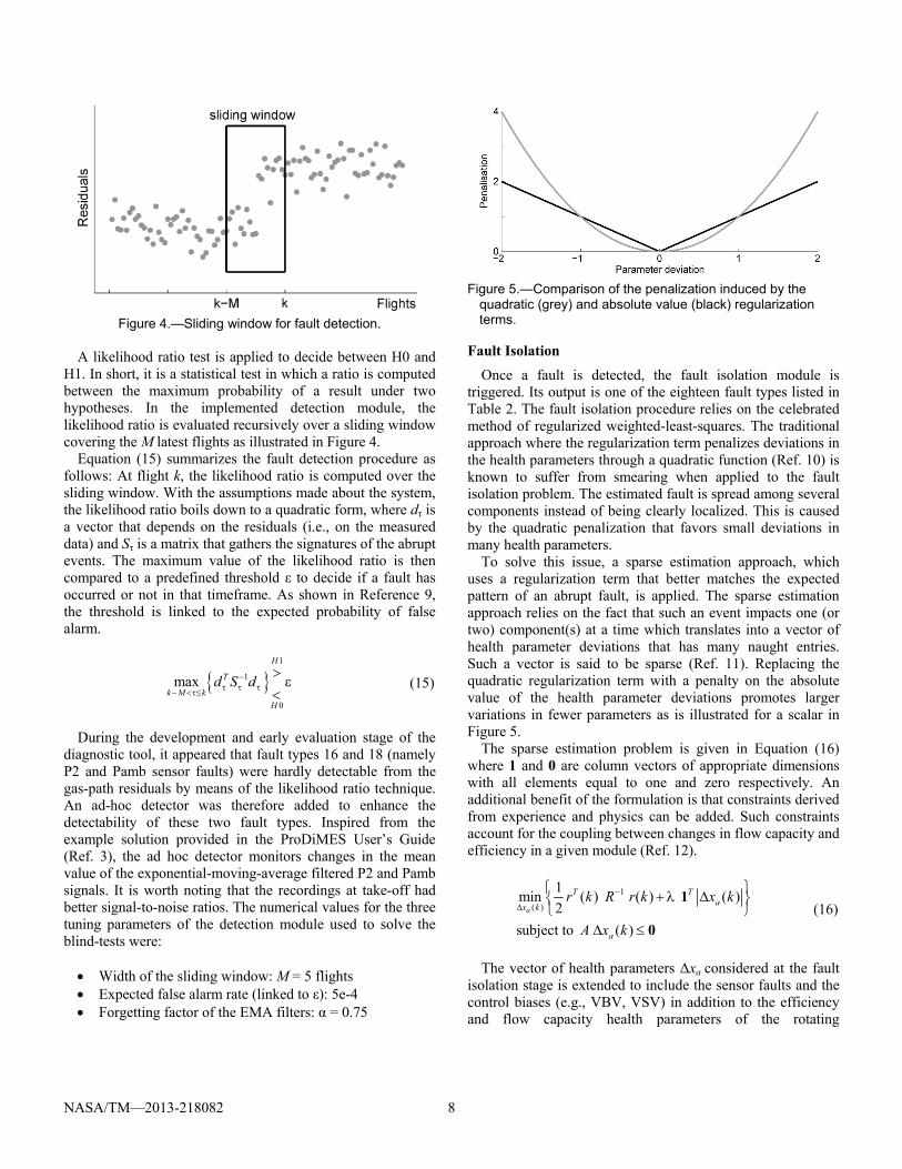
Figure 4.—Sliding window for fault detection.

A likelihood ratio test is applied to decide between H0 and

H1. In short, it is a statistical test in which a ratio is computed between the maximum probability of a result under two hypotheses. In the implemented detection module, the likelihood ratio is evaluated recursively over a sliding window covering the M latest flights as illustrated in Figure 4.

Equation (15) summarizes the fault detection procedure as follows: At flight k, the likelihood ratio is computed over the sliding window. With the assumptions made about the system, the likelihood ratio boils down to a quadratic form, where dτ is a vector that depends on the residuals (i.e., on the measured data) and Sτ is a matrix that gathers the signatures of the abrupt events. The maximum value of the likelihood ratio is then compared to a predefined threshold ε to decide if a fault has occurred or not in that timeframe. As shown in Reference 9, the threshold is linked to the expected probability of false alarm.

1

1

0

max

H

T

k M k

H

d S d

(15)

During the development and early evaluation stage of the

diagnostic tool, it appeared that fault types 16 and 18 (namely P2 and Pamb sensor faults) were hardly detectable from the gas-path residuals by means of the likelihood ratio technique. An ad-hoc detector was therefore added to enhance the detectability of these two fault types. Inspired from the example solution provided in the ProDiMES User’s Guide (Ref. 3), the ad hoc detector monitors changes in the mean value of the exponential-moving-average filtered P2 and Pamb signals. It is worth noting that the recordings at take-off had better signal-to-noise ratios. The numerical values for the three tuning parameters of the detection module used to solve the blind-tests were: Width of the sliding window: M = 5 flights Expected false alarm rate (linked to ε): 5e-4 Forgetting factor of the EMA filters: α = 0.75

Figure 5.—Comparison of the penalization induced by the

quadratic (grey) and absolute value (black) regularization terms.

Fault Isolation

Once a fault is detected, the fault isolation module is triggered. Its output is one of the eighteen fault types listed in Table 2. The fault isolation procedure relies on the celebrated method of regularized weighted-least-squares. The traditional approach where the regularization term penalizes deviations in the health parameters through a quadratic function (Ref. 10) is known to suffer from smearing when applied to the fault isolation problem. The estimated fault is spread among several components instead of being clearly localized. This is caused by the quadratic penalization that favors small deviations in many health parameters.

To solve this issue, a sparse estimation approach, which uses a regularization term that better matches the expected pattern of an abrupt fault, is applied. The sparse estimation approach relies on the fact that such an event impacts one (or two) component(s) at a time which translates into a vector of health parameter deviations that has many naught entries. Such a vector is said to be sparse (Ref. 11). Replacing the quadratic regularization term with a penalty on the absolute value of the health parameter deviations promotes larger variations in fewer parameters as is illustrated for a scalar in Figure 5.

The sparse estimation problem is given in Equation (16) where 1 and 0 are column vectors of appropriate dimensions with all elements equal to one and zero respectively. An additional benefit of the formulation is that constraints derived from experience and physics can be added. Such constraints account for the coupling between changes in flow capacity and efficiency in a given module (Ref. 12).

1

( )

1min ( ) ( ) ( )

2

subject to ( )

a

T Ta

x k

a

r k R r k x k

A x k

1

0

(16)

The vector of health parameters Δxa considered at the fault

isolation stage is extended to include the sensor faults and the control biases (e.g., VBV, VSV) in addition to the efficiency and flow capacity health parameters of the rotating

NASA/TM—2013-218082 9

components. As a result, the sparse estimation problem uses a fault influence coefficient matrix Ha that aggregates the matrix H used in the Kalman filter and the signatures of the sensor and control biases on the gas-path measurements.

( ) ( ) ( )a ar k y k H x k (17)

From a computational point of view, the sparse estimation problem is formulated as a Quadratic Programming problem for which efficient off-the-shelf solvers are available. The tuning parameter λ that trades off sparsity in the solution and fit of the data was set to a value of one. To determine the fault type from the sparse estimate, a simple isolation logic is applied. It assumes that only one component is faulty at a time. The magnitude of each fault type is calculated from the estimated deviations in the health parameters. The entity with the largest magnitude is deemed as the faulty one.

Diagnostic Method #4—Generalized Observer/Estimator for Single Fault Isolation

The fourth diagnostic method was developed by Wright State University. It begins by considering the linear state space representation of the engine model given as:

x Ax Bu Ef

y Cx Du Ff

(18)

where x is the state vector (i.e., Nf and Nc), u is the input vector (i.e., Wf, VSV, and VBV), y is the output vector, f is the fault vector, and A, B, C, D, E, and F are matrices of appropriate dimensions. Specifically, E, and F are the fault distribution matrices (Ref. 13). It is worth noting that the dimension of the fault vector f depends on the specific fault type under consideration. In the case of a component fault,

2f represents the changes in efficiency and flow capacity;

in the case of an actuator fault, f represents the actuator

bias; and in the case of a sensor fault, f represents the

sensor bias (note that E = [0 0]T in this case). The state space engine model described by Equation (18) can be equivalently represented as

( )y s G s u s H s f s (19)

where 1( ) ( )G s C sI A B D , and

1( ) ( )H s C sI A E F . Under steady-state operating

conditions as considered in ProDiMES, the model reduces to

Engine

FDEFault Detection

Decision Scheme

FIE Fan

FIE LPC

FIE HPC

…

FIE T2

FIE Pamb

Fault Isolation Decision Scheme

u y

Activation

Figure 6.—Diagnostic method #4 fault detection and isolation

architecture.

y Gu Hf (20)

where 1G CA B D and 1H CA E F . Although G

and H matrices are not directly available in analytical engine simulations such as the steady-state engine model provided in ProDiMES, they can be determined numerically.

The fault detection and isolation (FDI) architecture applied to ProDiMES consists of a fault detection estimator (FDE) and a bank of fault isolation estimators (FIEs), as shown in Figure 6. The FDE is used for detecting the occurrence of a fault, while the bank of FIEs is employed to determine the particular fault type after fault detection. Below, we detail the FDI method and then the FIE method.

Fault Detection Method

Based on the steady-state engine model given by Equation (20), the fault detection residual is defined as z y Gu . In addition to the seven residual components

considered in the example solution (Ref. 3), two additional residual components are used to enhance detection performance. One of them represents the deviation between the sensed Nf measurement and an Nf estimate obtained by balancing the steady-state engine model to the sensed Nc measurement. The other residual component captures abnormal Mach due to sensor faults in Pamb and P2 by comparing the estimated Mach with the average Mach in the first 10 flights. Each of these nine residual components is filtered and compared with a pre-defined threshold for detecting the occurrence of a fault. For simplicity, the effect of normal engine degradation on the diagnostic residual is considered as the average of each residual component during the first 10 flights, which are known to be fault free.

NASA/TM—2013-218082 10

Fault Isolation Method

After a fault is detected, the FIEs are activated to determine the particular fault type that has occurred. Each isolation estimator is designed based on the fault type under consideration.

The FIEs corresponding to engine component faults and actuator faults are designed based on adaptive estimation techniques (Ref. 13). Based on the steady-state engine model given by Equation (20), the FIE corresponding to each component fault or actuator fault is chosen as follows: for i = 1, 2, …, 8,

( ) ( ) ( ) ( )

ˆ ˆ( 1) ( ) ( )

i i i

Ti i i i i

k y k Gu k H f k

f k f k H k

(21)

where k is the engine flight number, ˆif is the estimated fault

magnitude generated by the ith FIE (i.e., estimated changes in the efficiency and flow capacity in the case of component faults, and estimated bias in the case of actuator faults), iH is a

fault functional matrix corresponding to the ith fault, i is a

learning rate, and i is the output estimation error used as the

residual for fault isolation. It is worth noting that if the fault functional matrices iH are sufficiently different for different

fault types, then in the presence of a particular component or actuator fault, the residual generated by the corresponding FIE should be the smallest one.

The FIEs corresponding to sensor faults are designed based on the generalized observer scheme (Ref. 14). Specifically, the FIE corresponding to a particular sensor fault is designed by utilizing all eight sensor signals except the particular sensor under consideration. For instance, the FIE corresponding to the Nf sensor fault utilizes all eight engine output measurements

except the Nf signal, as shown in Figure 7, where Nc represents an estimate of the Nc sensor signal, and so on. The fault isolation residual generated by the Nf FIE is defined as the deviation between the actual sensor measurements and their estimates provided by the FIE. Analogously, the FIE corresponding to the Nc sensor fault utilizes all eight engine output measurements except the Nc signal. Thus, in the presence of a particular sensor fault, because only the inputs to the corresponding FIE are not affected, the residual associated with the corresponding FIE should remain the smallest (in the absence of modeling uncertainty).

The fault isolation decision logic follows that of the generalized observer scheme (Ref. 14). Specifically, the fault type corresponding to the FIE with the smallest residual is considered to be the one that has occurred. Since it is not feasible to design normal observers for the sensor FIEs, they are implemented numerically. For instance, the Nf sensor fault FIE shown in Figure 7 is implemented by balancing the steady-state engine model to a power condition where the model’s Nc output is equivalent to the sensed Nc measurement.

NfFault

IsolationEstimator

Nc

P24

Wf

.

.

.

Nc

P24

Wf

.

.

.

Figure 7.—Structure of FIE for Nf sensor fault.

Similarly, the Nc sensor fault FIE is implemented by balancing the steady-state engine model to a power condition where the model’s Nf output is equivalent to the sensed Nf measurement.

The fault isolation algorithms for sensor faults in P2, T2, and Pamb are designed with special care because these signals are used for parameter correction purpose. Specifically, the FIE corresponding to the T2 sensor fault is designed as if it were a component fault. Additionally, the sensor faults in P2 and Pamb are isolated by monitoring anomalies in the Mach estimate and P2 measurement compared with their averages of the first ten flights.

Blind-Test-Case Metric Results

Developers of the diagnostic methods submitted their blind-test-case results to NASA for evaluation using the ProDiMES metrics routine. An abbreviated presentation of the results is provided in the subsections.

False Positive Rate

The false positive rate (FPR) results for the four diagnostic methods are shown in Table 3. This was calculated by counting the total number of flights where a nominal engine was erroneously declared faulty and dividing this quantity by the total number of nominal flights. The inverse of FPR, which is shown in the last column of Table 3, reflects the average number of flights required to generate a false positive for each algorithm. All four algorithms satisfied the requirement of no more than one false alarm per 1000 flights. Furthermore, diagnostic methods #1 and #2, which apply the same fault detection logic, exhibit identical FPR results.

TABLE 3.—FALSE POSITIVE RATE (FPR) Diagnostic

method FPR,

percent (Average # flights per false alarm)

1 and 2 0.09203 1087 3 0.09240 1082 4 0.09352 1069

NASA/TM—2013-218082 11

TABLE 4.—TRUE POSITIVE RATE (TPR) Diagnostic method TPR,

percent 1 and 2 44.7

3 50.9 4 51.9

Figure 8.—True positive rate.

True Positive Rate

Overall true positive rate (TPR) results considering all fault types, evolution rates, and magnitudes are shown in Table 4. Figure 8 shows a further breakdown of TPR results according to fault evolution rate (abrupt and rapid) and fault magnitude (small, medium, large). As expected, these results reveal that abrupt faults are easier to detect than rapid faults for a given fault magnitude, and that fault detection performance improves with increasing fault magnitude.

While none of the methods had an exceptionally high TPR, this was somewhat expected due to the flight history windows defined for applying the metrics. Specifically, TPR was assessed over all flights contained in each faulty engine’s “fault window” (10 flights for abrupt faults and 15 flights for rapid faults). Achieving a perfect TPR score would have required that every fault was correctly detected on all flights within the fault window. However, in most cases there was some latency associated with the correct detection of a fault resulting in missed detections during the first few flights within a fault window. This detection latency, which will be discussed in the section, reduces the TPR results.

Detection Latency

Overall average detection latency results considering all fault types, evolution rates, and magnitudes are shown in Table 5. A further breakdown of detection latency results according to fault evolution rate and fault magnitude is shown in Figure 9. Typically, abrupt faults are detected with less latency than rapid faults, and detection latency is reduced with increasing fault magnitude. While the detection approach applied by diagnostic method #1 and #2 exhibits the longest

TABLE 5.—DETECTION LATENCY Diagnostic method Latency (average # flights)

1 and 2 4.86 3 4.02 4 4.24

Figure 9.—Detection latency.

TABLE 6.—KAPPA COEFFICIENT

Diagnostic method Kappa coefficient 1 0.588 2 0.590 3 0.627 4 0.617

Figure 10.—Kappa coefficient.

detection latency, it is interesting to note that diagnostic method #3 exhibits slightly superior diagnostic latency when compared to diagnostic method #4. Previously, diagnostic method #4 was shown to have better TPR performance than diagnostic method #3.

Kappa Coefficient

Kappa coefficient results for the four diagnostic methods are shown in Table 6 and Figure 10. Since Kappa coefficient is a reflection of fault classification performance, diagnostic

All Small Medium Large0

20

40

60

80

100

TP

R (

%)

Abrupt Faults

All Small Medium Large0

20

40

60

80

100

TP

R (

%)

Rapid Faults

Fault Magnitude

Diagnostic method #1Diagnostic method #2Diagnostic method #3Diagnostic method #4

All Small Medium Large0

5

10

Late

ncy

(flig

hts)

Abrupt Faults

All Small Medium Large0

5

10

Late

ncy

(flig

hts)

Rapid Faults

Fault Magnitude

Diagnostic method #1Diagnostic method #2Diagnostic method #3Diagnostic method #4

All Small Medium Large0

0.2

0.4

0.6

0.8

1

Ka

ppa

coe

ffici

ent Abrupt Faults

All Small Medium Large0

0.2

0.4

0.6

0.8

1

Kap

pa c

oef

ficie

nt

Abrupt Faults

Fault Magnitude

Diagnostic method #1Diagnostic method #2Diagnostic method #3Diagnostic method #4

NASA/TM—2013-218082 12

methods #1 and #2 exhibit different results as they apply different classifiers. Diagnostic method #3 has the highest Kappa coefficient score, followed by diagnostic methods #4, #2, and #1.

Correct Classification Rate and Mis-Classification Rate

The correct classification rate (CCR) and mis-classification (MCR) results for the four diagnostic methods are shown in Table 7. Although similar for all four methods, diagnostic method #3 has the highest CCR, followed by diagnostic methods #4, #2, and #1—the same ranked ordering of methods as was found for the Kappa coefficient. The MCR results, which are TPR minus CCR, shows that diagnostic method #2 produces the fewest misclassifications followed by methods #1, #3, and #4.

A further breakdown of the CCR per individual fault type is shown in Figure 11. In general, faults such as HPC, HPT, LPT, and VSV are readily diagnosable by all algorithms while other faults such as LPC, VBV, Nc, P2 and Pamb proved to be more challenging to diagnose.

Discussion of Blind-Test-Case Metric Results

A summary of the blind-test-case metric results is given in Table 8, which shows the ranking of the diagnostic methods for each metric.

A critical aspect in benchmarking and comparing the performance of different diagnostic methods is the need to establish some measure of commonality. The blind test comparison included in ProDiMES attempts to establish this commonality by specifying a required false alarm rate of no more than one false alarm per 1000 flights (i.e., FPR 0.1 percent). However, at this relatively low FPR level, even small changes in FPR can have a large effect on other metric results. In light of this, all of the evaluated methods were designed to exhibit fairly similar FPR rates ranging from one false positive every 1069 to 1087 flights. This similarity in FPR was intentional as the initial submission defined an ad hoc FPR target that the remaining submissions then attempted to match to enable a “fair” comparison. Ideally, it would have been desirable to iteratively adjust the detection thresholds of each method to achieve closer FPR matching, but this was not practical given the ProDiMES setup.

Also noted is the inherent coupling between fault detection and fault classification performance. Obviously, a fault must first be detected before it can be classified and this fact is reflected in the metric results. The fault detection technique applied in diagnostic methods #1 and #2 has the lowest TPR, detecting 6.2 and 7.2 percent fewer faults than diagnostic methods #3 and #4, respectively. Diagnostic methods #1 and #2 also exhibit lower CCR and Kappa coefficient performance compared to the other two methods. However, the disparity in terms of classification performance is not as large. The

TABLE 7.—CORRECT CLASSIFICATION RATE (CCR) AND MIS-CLASSIFICATION RATE (MCR)

Diagnostic method

CCR, percent

MCR, percent

1 43.4 1.35 2 43.7 1.04 3 46.7 4.15 4 45.2 6.78

Figure 11.—Correct classification rate.

TABLE 8.—DIAGNOSTIC METHOD RANKING

FOR EACH METRIC Diag.

method FPR rank

TPR rank

Detect. latency

rank

Kappa coeff. rank

CCR rank

MCR rank

1 3rd 3rd 3rd 4th 4th 2nd 2 3rd 3rd 3rd 3rd 3rd 1st 3 2nd 2nd 1st 1st 1st 3rd 4 1st 1st 2nd 2nd 2nd 4th

difference between the highest (diagnostic method #3) and lowest (diagnostic method #1) performing method in terms of CCR is only 3.3 percent, which is about 50 percent less than the disparity in TPR. Also noted is the fact that diagnostic methods #1 and #2 exhibit fewer misclassifications than diagnostic methods #3 and #4 (Table 7). The reasons for this are not clear. One possibility may be that the classifiers contained in diagnostic methods #1 and #2 perform better when applied to ProDiMES. Another possibility may be that diagnostic methods #3 and #4 are detecting smaller magnitude faults with reduced latency, which in turn yields fault signatures with lower signal to noise ratios. This would make fault classification more challenging, resulting in more misclassifications. Without further analysis it is not possible to definitively interpret all of the classification results. However, follow on work comparing the results obtained by pairing different classifier approaches with the best performing detection approaches is a recognized area of interest.

Recall that diagnostic methods #3 and #4 include additional logic to help improve the diagnosis of P2 and Pamb sensor faults. These fault events exhibit low signal to noise ratios within ProDiMES making them challenging to accurately

Fan LPC HPC HPT LPT VSV VBV Nf Nc P24 Ps30 T24 T30 T48 Wf P2 T2 Pamb0

20

40

60

80

100

CC

R (

%)

Abrupt faults

Fan LPC HPC HPT LPT VSV VBV Nf Nc P24 Ps30 T24 T30 T48 Wf P2 T2 Pamb0

20

40

60

80

100

CC

R (

%)

Rapid faults

Diagnostic method #1Diagnostic method #2Diagnostic method #3Diagnostic method #4

NASA/TM—2013-218082 13

diagnose. The fault classification results in Figure 11 show that these two methods perform much better than diagnostic methods #1 or #2 in terms of diagnosing Pamb faults, and diagnostic method #4 outperforms all other methods in diagnosing P2 faults. This suggests that adding additional logic can indeed be beneficial in helping improve the diagnosis of certain fault types.

Other interesting findings are revealed by comparing the results of diagnostic methods #1 and #2, which apply the same fault detection approach but different fault classification techniques. Diagnostic method #1 applies a model-based (analytical) weighted least squares (WLS) approach while diagnostic method #2 applies a data-driven (empirical) probabilistic neural network (PNN) approach. Development of the WLS approach is slightly more complicated as it requires the generation of a fault influence coefficient matrix from an analytical model, while implementation of the PNN approach is more computationally complex. When applied to the ProDiMES blind-test-case data these two methods are found to produce very similar fault classification results. The Kappa coefficient results only differ by 0.002, and CCR results by 0.3 percent, with the PNN approach of diagnostic method #2 holding the slight advantage. Prior to running this comparison, the PNN approach was expected to have a couple of distinct advantages over the WLS approach. This includes the ability of the PNN approach to capture system non-linear behavior as opposed to the WLS approach, which is strictly linear in nature, and the ability of the PNN to recognize uni-direction fault signatures. For example, the five turbomachinery faults implemented in ProDiMES (i.e., Fan, LPC, HPC, HPT, and LPT) always result in an engine performance decrease, never an increase. While the PNN is trained to recognize this fact, no logic is included in the WLS approach to guard against diagnosing turbomachinery faults that produced an observed performance increase, which would likely lead to a fault misclassification. However, system nonlinearities and lack of uni-directional fault logic did not prove to be a significant limitation for the WLS approach. Decisions to implement analytical versus empirical classification approaches on data sets exhibiting similar behavior as ProDiMES may largely depend on what information is available (e.g., accurate models versus adequate quantities of fault data for training purposes).

Lessons Learned and Recommendations for Improvement

At the ProDiMES workshop, attendees were asked to provide feedback and recommendations on improving the ProDiMES tool and the public EHM benchmarking process in general. Participant feedback on the ProDiMES software tool itself was generally positive. The tool was found to present a suitably challenging gas path diagnostic benchmark problem, and the ProDiMES software was acknowledged as user friendly while providing most of the desired functionality. The ability to apply and assess diagnostic methods against a

standard and credible benchmark problem from a trusted source was an acknowledged benefit. The standard metrics and terminology defined by ProDiMES were also positively noted.

Some of the recommendations for improvement included adding more realism to the problem. This includes incorporating more realistic measurement uncertainty such as outliers, data dropouts, analog-to-digital conversion digitization effects, and more realistic covariance between the sensor measurements. Flight-to-flight variations in operating conditions based on actual flight data and more realistic fault magnitudes were also recommended. In terms of the problem setup itself, a recommendation was made to reduce the number of gas path sensors to be more representative of measurement suites typically available. In particular, the measurements at the LPC exit (i.e., P24 and T24) are often unavailable. Also, it was recommended to provide data at a single cruise operating point and omit the takeoff data. Other suggested enhancements were to include intermittent fault types, overhaul or maintenance events that resulted in a restoration of engine performance, and to permit the occurrence of multiple faults within an individual engine.

In terms of the public benchmarking process itself, attendees acknowledge that without funding resources and organizational support, it is difficult to develop and apply a diagnostic method to the problem. One workshop attendee did express the following reservation regarding participation: Although the process was not setup as a “competition,” there is no way to avoid the fact that the performance of different participants is compared. It was noted that several conferences have recently begun putting forth annual diagnostic or prognostic challenge problems. Offering ProDiMES to serve as a conference challenge problem was suggested as a means to gain more end users of the tool.

Summary

An overview of a publicly available aircraft engine gas path diagnostic benchmark problem has been presented along with the results of four diagnostic methods applied to this problem. The results of this benchmarking exercise demonstrate the importance of accurate fault detection as the diagnostic methods with the best fault detection performance also achieved the best correct classification performance. Follow on work to pair classification techniques with the best detection techniques is a recommended area of future study. The benchmark problem was found to enable the application of both analytical and empirical diagnostic methods, which were found to yield comparable diagnostic performance. Overall participant feedback on the benchmark tool and process was generally positive. Recommendations for improvement included adding more realism to the problem setup and coupling with a conference challenge problem to gain broader participation.

NASA/TM—2013-218082 14

References

1. Jaw, L.C., 2005, “Recent Advances in Aircraft Engine Health Management (EHM) Technologies and Recommendations for the Next Step,” ASME Paper GT2005-68625.

2. The Technical Cooperation Program (TTCP) Website: http://www.acq.osd.mil/ttcp/, accessed January 9, 2013.

3. Simon, D.L., 2010, “Propulsion Diagnostic Method Evaluation Strategy (ProDiMES) User’s Guide,” NASA/TM—2010-215840.

4. Volponi, A.J., et al., 2003, “Gas Turbine Condition Monitoring and Fault Diagnostics,” Von Kármán Institute Lecture Series, VKI LS 2003-01, Rhode-Saint-Genèse, Belgium.

5. Volponi, A.J., 1999, “Gas Turbine Parameter Corrections,” ASME J. of Engineering for Gas Turbines and Power, Vol. 121, pp. 613–621.

6. DePold, H.R., Gass, F.D., 1999, “The Application of Expert Systems and Neural Networks to Gas Turbine Prognostics and Diagnostics,” ASME J. of Engineering for Gas Turbines and Power, Vol. 121, pp. 607-612.

7. Demuth, H., Beale, M. “Neural Network Toolbox For Use With MATLAB,” Version 4, The MathWorks, Natick, MA, 1992, Chap. 7.

8. Kobayashi T., Simon D.L., Litt J.S., 2005, “Application of a Constant Gain Extended Kalman Filter for in-flight Estimation of Aircraft Engine Performance Parameters,” ASME Paper GT2005-68494.

9. Borguet S., Léonard O., 2009, “A Generalized Likelihood Ratio Test for Adaptive Gas Turbine Performance Monitoring,” ASME J. of Engineering for Gas Turbines and Power, 131:011601.

10. Doel D.L., 1994, “An Assessment of Weighted-Least-Squares-Based Gas Path Analysis,” ASME J. of Engineering for Gas Turbines and Power, 116, pp. 366-373.

11. Borguet S., Léonard O., 2010, “A Sparse Estimation Approach to Fault Isolation,” ASME J. of Engineering for Gas Turbines and Power, 132:021601.

12. Borguet S., Léonard O., 2011, “Constrained Sparse Estimation for Improved Fault Isolation,” ASME J. of Engineering for Gas Turbines and Power, 133:121602.

13. Ioannou, P.A., and Sun, J., 1996, Robust adaptive control, Englewood Cliffs, NJ: Prentice Hall.

14. Chen, J., and Patton, R.J., 1999, Robust Model-Based Fault Diagnosis for Dynamic Systems, London: Kluwer Academic Publishers.

REPORT DOCUMENTATION PAGE Form Approved OMB No. 0704-0188

The public reporting burden for this collection of information is estimated to average 1 hour per response, including the time for reviewing instructions, searching existing data sources, gathering and maintaining the data needed, and completing and reviewing the collection of information. Send comments regarding this burden estimate or any other aspect of this collection of information, including suggestions for reducing this burden, to Department of Defense, Washington Headquarters Services, Directorate for Information Operations and Reports (0704-0188), 1215 Jefferson Davis Highway, Suite 1204, Arlington, VA 22202-4302. Respondents should be aware that notwithstanding any other provision of law, no person shall be subject to any penalty for failing to comply with a collection of information if it does not display a currently valid OMB control number. PLEASE DO NOT RETURN YOUR FORM TO THE ABOVE ADDRESS.

1. REPORT DATE (DD-MM-YYYY) 01-11-2013

2. REPORT TYPE Technical Memorandum

3. DATES COVERED (From - To)

4. TITLE AND SUBTITLE Aircraft Engine Gas Path Diagnostic Methods: Public Benchmarking Results

5a. CONTRACT NUMBER

5b. GRANT NUMBER

5c. PROGRAM ELEMENT NUMBER

6. AUTHOR(S) Simon, Donald, L.; Borguet, Sebastien; Leonard, Olivier; Zhang, Xiaodong (Frank)

5d. PROJECT NUMBER

5e. TASK NUMBER

5f. WORK UNIT NUMBER WBS 284848.02.04.03.02.01

7. PERFORMING ORGANIZATION NAME(S) AND ADDRESS(ES) National Aeronautics and Space Administration John H. Glenn Research Center at Lewis Field Cleveland, Ohio 44135-3191

8. PERFORMING ORGANIZATION REPORT NUMBER E-18768

9. SPONSORING/MONITORING AGENCY NAME(S) AND ADDRESS(ES) National Aeronautics and Space Administration Washington, DC 20546-0001

10. SPONSORING/MONITOR'S ACRONYM(S) NASA

11. SPONSORING/MONITORING REPORT NUMBER NASA/TM-2013-218082

12. DISTRIBUTION/AVAILABILITY STATEMENT Unclassified-Unlimited Subject Category: 07 Available electronically at http://www.sti.nasa.gov This publication is available from the NASA Center for AeroSpace Information, 443-757-5802

13. SUPPLEMENTARY NOTES

14. ABSTRACT Recent technology reviews have identified the need for objective assessments of aircraft engine health management (EHM) technologies. To help address this issue, a gas path diagnostic benchmark problem has been created and made publicly available. This software tool, referred to as the Propulsion Diagnostic Method Evaluation Strategy (ProDiMES), has been constructed based on feedback provided by the aircraft EHM community. It provides a standard benchmark problem enabling users to develop, evaluate and compare diagnostic methods. This paper will present an overview of ProDiMES along with a description of four gas path diagnostic methods developed and applied to the problem. These methods, which include analytical and empirical diagnostic techniques, will be described and associated blind-test-case metric results will be presented and compared. Lessons learned along with recommendations for improving the public benchmarking processes will also be presented and discussed. 15. SUBJECT TERMS Systems health monitoring; Gas turbine engines

16. SECURITY CLASSIFICATION OF: 17. LIMITATION OF ABSTRACT UU

18. NUMBER OF PAGES

22

19a. NAME OF RESPONSIBLE PERSON STI Help Desk (email:help@sti.nasa.gov)

a. REPORT U

b. ABSTRACT U

c. THIS PAGE U

19b. TELEPHONE NUMBER (include area code) 443-757-5802

Standard Form 298 (Rev. 8-98)Prescribed by ANSI Std. Z39-18