Air Quality Data

A New Conceptual Approach

Outline

GoalPresent ConceptProblemsNew ConceptAdvantagesApproachNetwork DesignExample Application

Basic Goal

Produce a complete SPATIAL picture of air quality in a cost effective manner with acceptable uncertainty

Present Concept

Air Quality Data (AQD) are truth (no uncertainty)

BUTBUT:: Where there are no monitors there is no information

Problems With the Present ConceptAQD “truth” is simply what a monitor recorded at a specific place and time. Its relevance and certainty depend on its use and instrument error.We use monitored AQD to represent unmonitored areas (i.e., 10 ft. from the monitor) – WE ESTIMATE!To use AQD we must create a spatial picture (implicit interpolation) – e.g.:– AQD are representative of the entire area of the county in which

they are taken – AQD provide no information outside the county in which they are

takenFor a complete spatial picture monitors are needed everywhere (including counties that have monitors) -network optimization is meaninglessDisincentive to monitor

New ConceptAir Quality Concept:– Actual monitored or estimated (kriged) air quality

are the same except for uncertainty– Define air quality as a estimated field of actual

concentrations and their associated uncertaintiesEstimate Actual Concentration Field:– AQD are simply a sample of the “Actual” air quality– AQD are used as input to an interpolation model

(kriging) to estimate the actual concentration field– Use area modeling to establish the best variogram

for krigingEstimate uncertainty using area modeling

Advantages to New ConceptThe complete field of air quality is available for policy development, trends analysis, etc.The estimated concentration field is robust– Changes to an optimized network should not

significantly affect the estimates– Lack of county monitors does not result in NO data

Removes monitoring disincentiveProvides a direct blueprint for developing optimal cost-effective networks

Approach:Constructing actual concentration field:– Produce a BENCHMARK concentration field from

area modeling (modeling data must adequately characterize important features of the field)

– Establish the best variogram model for the area using the benchmark data

– Estimate, through kriging, the actual concentration field using:• The variogram model constructed from the benchmark

data• All available monitored air quality values both within and

outside the area

Ozone Monitoring Network used for Kriging

1999 8hr. Ozone Design Value: Kriged Grid with Network Overlay

1999 Ozone Design Values: Kriged Contour Map

(ppb)

Approach (cont.):Constructing uncertainty field– Develop a subset of the benchmark (modeled)

data from monitor locations only– Estimate the actual concentration field by kriging

the benchmark data subset– Compare the full benchmark field with the

estimated field from the benchmark subset– Construct a field of residuals (the uncertainty field)

BENCHMARK Data Set4th High 8hr. Ozone: UAM-V Model Output

1996 Emissions Inventory30 Days of 1995 Met

(ppb)

Constructing Data Subset (modeled values at monitor locations) from Benchmark UAM-V Modeling

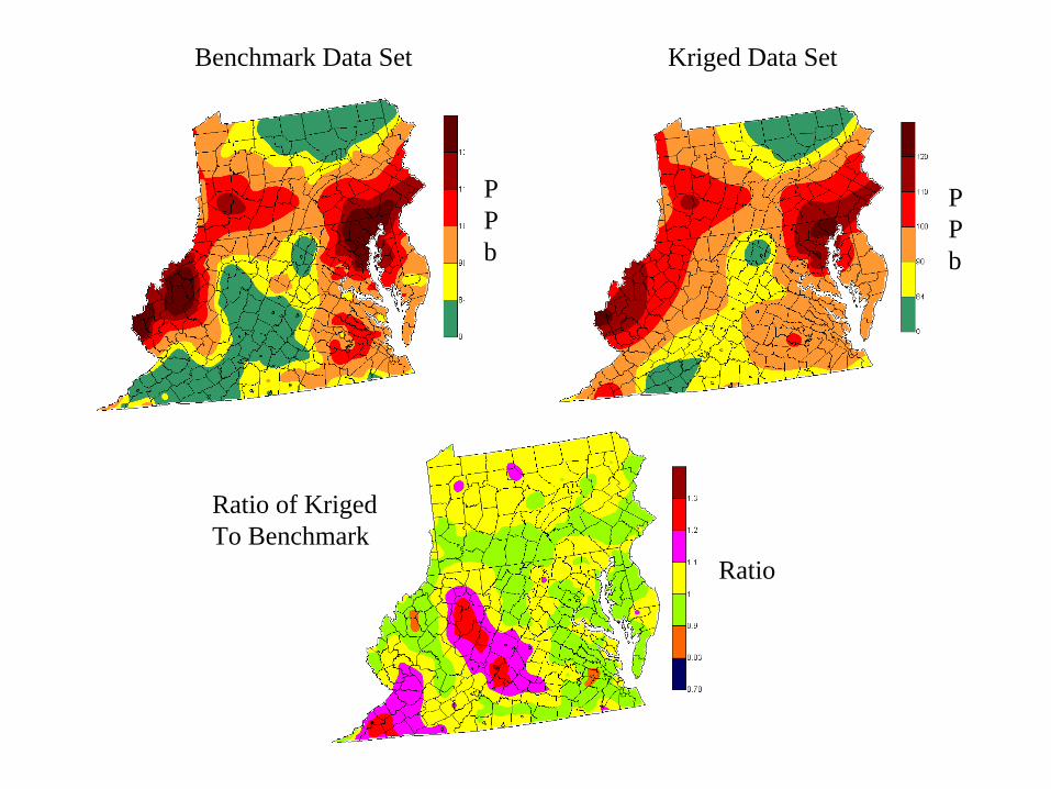
Benchmark Data Set Kriged Data Set

Ratio of KrigedTo Benchmark

Ratio

PPb

PPb

Network Design

PREMISE: An optimum network is one that produces minimum uncertainty for acceptable resource demand.GENERAL APPROACH:– Develop a benchmark (modeled) concentration

field– Construct various data subsets from the

benchmark data (i.e., network designs)– Estimate (krig) a concentration field for each

network design

Network Design (cont.)GENERAL APPROACH (cont.):– Compare each estimated field to the benchmark

field– Choice the best design: establish point of

diminishing returns– Example:

• Existing Network Corr Coeff = .89• Add monitor: Albemarle county Corr Coeff = .90• Add Albemarle & Harrison county Corr Coeff = .91

Ratio of KrigedTo Benchmark

Existing Network (Corr Coeff = 0.89) Add Albemarle (Corr Coeff = 0.90)

*

Add Harrison(Corr Coeff = 0.91)

*

*

Ratio of Kriged to Benchmark: Black = Present Network; Red = + Albemarle; Blue = + Harrison

Network Design (cont.)Plan for Optimizing Present Network– Develop appropriate benchmark data set (use existing modeled

data if possible)– Develop the best variogram model for kriging– Develop optimization criteria

• Comparison statistics: Correlation Coefficient; Maximum residual; Etc.• Resource demand• State preference• Etc.

– Compare Benchmark with estimated “present network” field : establish baseline stats.

– Optimize Network• Create potential new network

– Examine uncertainty (residual) fields– Remove &/or add monitors

• Compare new network with Baseline • Iterate to find optimal network

Application of New ApproachUse of Interpolated AQ for Region III 8hr. Ozone Attainment DesignationsPROCEDURE:– Estimate 1999 8hr. Ozone design value for all counties– Establish uncertainty field (benchmark – kriged)

• UAMV modeled 4th high 8 hr. average– 1996 base emissions– 30 days met 1995 – several episodes

– Weight estimate by uncertainty• The larger the residual the less weight the given to the estimate• Consider counties with monitors to be considerably more

reliable than counties without (to reflect present EPA bias)