Air pollution Dr. Yasmen A. Mustafa Assistant professor in Environmental Engineering Department College of Engineering /Baghdad University

Air Pollution Definition Atmospheric condition in which substances are present at concentration higher than their normal ambient (clean atmospheric) levels to produce significant effects on human, animals, vegetation or materials. The substances present may be any natural or man-made chemical elements or compounds in gaseous, liquid or solid stat that are capable of being airborne.

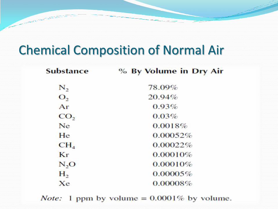
Chemical Composition of Normal Air

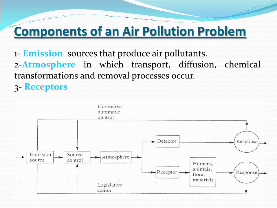
Components of an Air Pollution Problem

1- Emission sources that produce air pollutants. 2-Atmosphere in which transport, diffusion, chemical transformations and removal processes occur. 3- Receptors

Type and Scale of Air Pollution Problem

Type of

problem

Horizontal

scale

Vertical

scale

Temporal

scale

Type of

organization

Indoor

Local

Urban

10 -100 m

100m -10 km

10-102 km

Up to100 m

Up to 3km

Up to 3km

10-1 -100 hr

10-1 -10 hr

100 -102 hr

Family/business

Municipality/county

Municipality/county

Regional

continental

102 -103 km

103 -104 km

Up to 15 km

Up to 30 km

10 -103 hr

102 -104 hr

State/country

Country/world

Hemispheric

Global

104 - 2x104 km

4x104 km

Up to 50 km

Up to 50 km

103 -105 hr

103 -106 hr

World

world

Source: Modified after Stern et al.(1984)

Source of Air Pollution 1- Urban and industrial sources: -Power generation: Conventional fossil-fuel power plants are the major sources

of air pollution. Major sources for ( particulate matter including fly ash heavy metals,CO,CO2, SO2 ,NOx, volatile organic hydrocarbons (VOCs). Nuclear power plants are much cleaner in their normal operation, but accidental releases of radioactive substances are of great concern to the public.

-Industrial facilities: (mining , refining, manufacturing ,pharmaceutical -----etc).

Major sources for(all possible gases and particulate matter).

-Transportation:( mobile sources like automobiles ,buses ,trucks , airplanes ,

boats---etc). Major sources for (CO ,CO2 ,NOx ,SO2 , hydrocarbons(HCs ) ,VOCs ).

-Waste disposal: (urban household, commercial, and industrial waste products are

disposed of in landfills). Major sources for gaseous (e.g., CO, CO2, CH4, H2S and NH3).

-Process emissions: (furnaces and other processes used for heating and open

burning).Major sources for ( particulate matter and CO ,CO2 ,NOx ,SO2 , HCs ,VOCs).

-Construction activities: like land cleaning ,digging ,grinding ,paving , panting .

Major sources for(dust and other particulate matter ,HCs ,VOCs ,CO ,CO2 and Nox).

2-Agriculture and other rural sources:

-Dust blowing: (from tilling harvesting ---etc) .

-Slash burning: (land cleaning by burning).

-Soil emissions: (Treated soils with fertilizers emit nitrogen oxides produced by

microbial activity in the top most soil layer).

-Pesticides:(may attach in their transport a residential area).

-Decaying wastes:(Agriculture and animal waste decay release NH3 ,CH4

,noxious vapors to the atmosphere.)

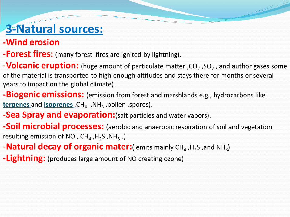
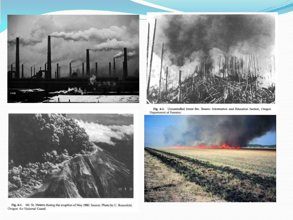
3-Natural sources: -Wind erosion

-Forest fires: (many forest fires are ignited by lightning).

-Volcanic eruption: (huge amount of particulate matter ,CO2 ,SO2 , and author gases some

of the material is transported to high enough altitudes and stays there for months or several years to impact on the global climate).

-Biogenic emissions: (emission from forest and marshlands e.g., hydrocarbons like

terpenes and isoprenes ,CH4 ,NH3 ,pollen ,spores).

-Sea Spray and evaporation:(salt particles and water vapors).

-Soil microbial processes: (aerobic and anaerobic respiration of soil and vegetation

resulting emission of NO , CH4 ,H2S ,NH3 .)

-Natural decay of organic mater:( emits mainly CH4 ,H2S ,and NH3)

-Lightning: (produces large amount of NO creating ozone)

Effects of Air Pollution -Effect on human health.

-Effect on vegetation and animals. -Effect on material and structures. -Atmospheric effects: -Visibility reduction: (especially from industrial plumes and urban smog). -Radiative effects: (The gaseous as well as particulate air pollutants in the atmosphere can significantly alter the radiation balance of the near surface layer. Particulate are most effective in reducing solar radiation , decrease of 10-20% in solar radiation due to air pollution have been observed over large cities). -Fog formation and precipitation: (Atmospheric particles can serve as nuclei for the condensation of water vapor, which is an important factor in the formation of fog and clouds). -Acid precipitation: (SO2 and NO2 undergo chemical transformation during their long range transport and produced acidic species entrained in the clouds making the resulting rain or snow more acidic). -Stratospheric ozone depletion: -Climate change: (Global warming or Green house effect due to the increases in radiatively active gases such as CO2 ,NH3 ,N2O and CFCs and tropospheric ozone).

Photochemical Smog

Photochemical Smog

Smog arises from photochemical reactions in the lower atmosphere by the

interaction of volatile organic compounds (VOCs) (total organic gases

minus methane) and nitrogen oxide (NOx) released by exhausts of

automobiles and some stationary sources.

This interaction result in series of complex reaction producing secondary

pollutants such as ozone(O3), aldehydes (RCHO), ketones (RCHO) and

peroxyacyl nitrates(PANs).

The most recognized gas-phase by-product of smog reactions is ozone

because ozone has harmful health effects and is an indicator of the presence

of other pollutants.

The conditions for the formation of photochemical smog are air

stagnation, abundant sun light, and high concentration of VOCs and NOx in

the atmosphere.

The reaction mechanisms are complex and are not fully understood.

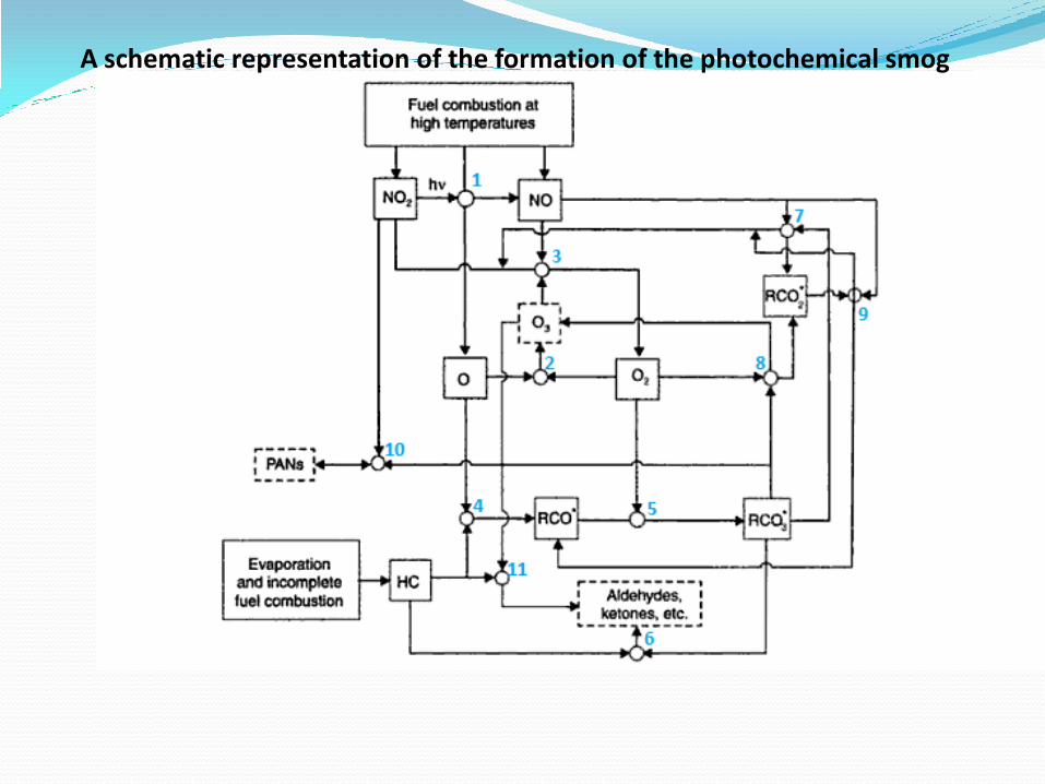
A schematic representation of the formation of the photochemical smog

Ozone isopleth

The ozone isopleth shows that, at low NOₓ, ozone is relatively

insensitive to VOC levels. At high NOₓ, an increase in VOC increases

ozone. At high VOC, increases in NO xalways increase ozone.

An isopleths is useful for regulatory control of ozone. In many polluted

urban areas, the VOC: NO x ratio is lower than 10:1, indicating that

limiting VOC emission should be the most effective method of controlling

ozone. Such a strategy was convenient because the control of VOC

emissions to the atmosphere was deemed to be technically an easier task

than controlling NOx emissions.

The relation between ozone and its precursors

In morning the (NO) and (HC) levels increases followed quickly by increase in

(NO2). NO2 react with the sun light leading to various chain reactions and

ultimately to the production of ozone and other oxidants. Ozone reach a

maximum at afternoon and then decreases gradually.

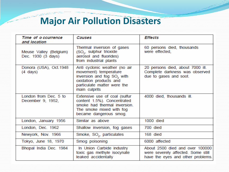
Major Air Pollution Disasters

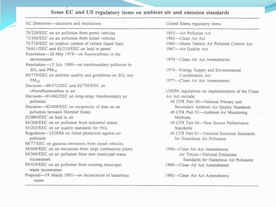
Regulatory Items on Ambient Air and Emission Standards

European Community (EC) air pollution standards began

in 1970 with emission standards for petrol vehicles. Prior to

1970 individual EC countries had their own standards. The reported death of 4000 people from London Smog in 1952 was the catalyst for the introduction of the UK clean air act in

1956 .in the United State (US) the air pollution control act

was introduced in 1955.

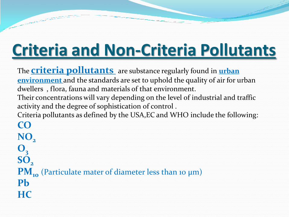
Criteria and Non-Criteria Pollutants The criteria pollutants are substance regularly found in urban

environment and the standards are set to uphold the quality of air for urban dwellers , flora, fauna and materials of that environment. Their concentrations will vary depending on the level of industrial and traffic activity and the degree of sophistication of control . Criteria pollutants as defined by the USA,EC and WHO include the following:

CO NO2 O3 SO2 PM10 (Particulate mater of diameter less than 10 µm)

Pb HC

AAQS for Criteria Pollutants in USA,EC and WHO

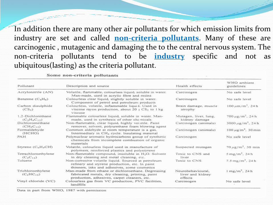
In addition there are many other air pollutants for which emission limits from industry are set and called non-criteria pollutants. Many of these are carcinogenic , mutagenic and damaging the to the central nervous system. The non-criteria pollutants tend to be industry specific and not as ubiquitous(lasting) as the criteria pollutant.

Air Quality standards There are two sets of air quality standards:

1. Ambient air Quality standards(AAQS)

2. Emission standards(ES)

Ambient air quality standards are prescriptive they are not based on

technological or economic acceptability they are depend on the effect of

air pollution on health and welfare.

There are two levels of AAQ`S

1. Primary AAQS for the protection of human health

2. Secondary AAQS for the protection of welfare (e.g., crops,

vegetation, buildings, visibility, etc.).

Six criteria air pollutants were specified by the EPA for NAAQS:

• Particulate

• Carbon monoxide (CO)

• Ozone (O3)

• Sulfur dioxide (SO2)

• Nitrogen dioxide (NO2)

• Lead

Volatile Organic Compounds (VOCs) are not considered as a criteria

pollutant, but they are regulated like a criteria pollutant because VOCs

and nitrogen oxides are precursors to ozone, which is produced by

photochemical reactions.

NAAQS Revisions (EPA)

The EPA was required to review the NAAQS every 5 years to ensure

that new research would be considered. The standard could remain at the

same level if the review proved that the standard provides sufficient

protection for health and welfare.

National Ambient Air Quality Standards(February 2001)

NAAQS as of February 2001 are listed in the below Table:

In 1997, the EPA issued a new primary and secondary ozone standard of 0.08

ppm for an 8-hour average in addition to the existing standard of 0.12 ppm for a 1-

hour average.

The EPA determined that longer-term exposures to lower levels of ozone caused

health effects including asthma attacks, breathing and respiratory problems, loss of

lung function, and possible long-term lung damage and decreased immunity to

disease. This was the first update of the ozone standard in 20 years.

Also in 1997, EPA established a new particulate matter standard for fine

particulates with an aerodynamic diameter of less than 2.5 microns PM2.5 . The

standard was established at 65µg/m3for a 24-hour average and 15 µg/m3for an

annual average.

National Ambient Air Quality Standards (as of October,2011)

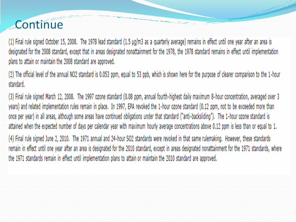
Continue

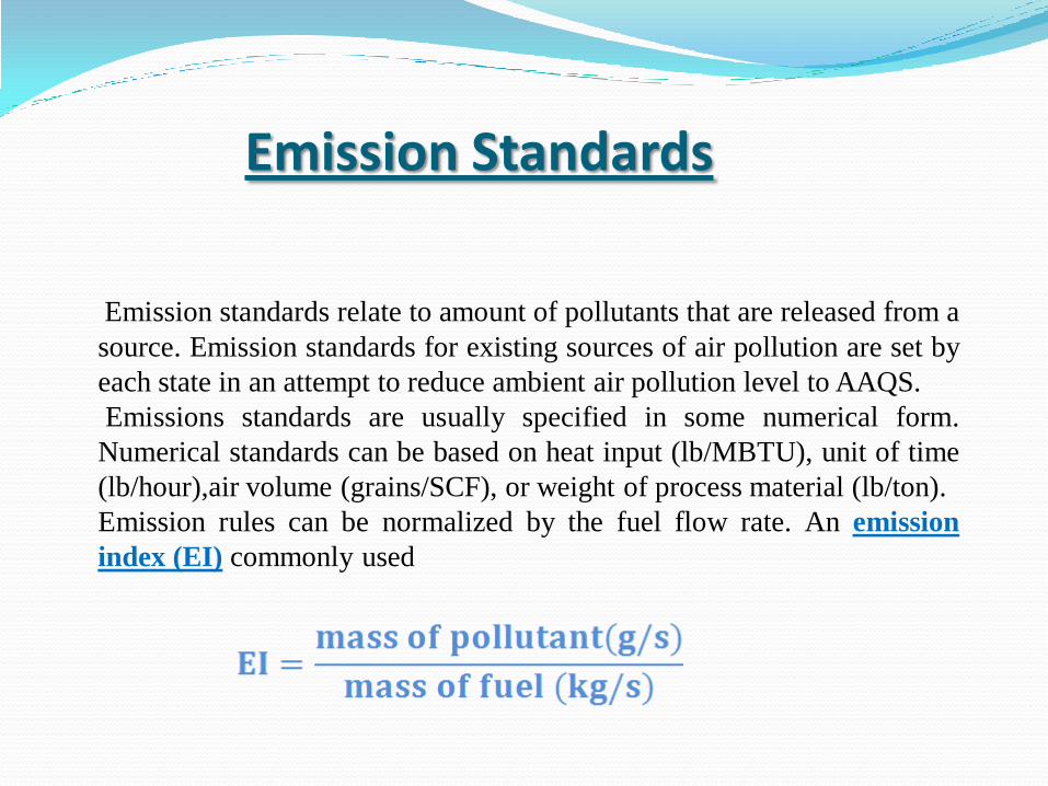
Emission Standards

Emission standards relate to amount of pollutants that are released from a

source. Emission standards for existing sources of air pollution are set by

each state in an attempt to reduce ambient air pollution level to AAQS.

Emissions standards are usually specified in some numerical form.

Numerical standards can be based on heat input (lb/MBTU), unit of time

(lb/hour),air volume (grains/SCF), or weight of process material (lb/ton).

Emission rules can be normalized by the fuel flow rate. An emission

index (EI) commonly used

Emission Assessment

Good quality source emission data are essential for effective

control of air pollution. Because of cost factors and the

complexities involved in source emissions determinations, this

aspect of air surveillance programs has not received the

attention it deserves.

Source Sampling

A variety of approaches may be used to determine emission

rates for a given source. The most desirable means is to actually

measure emissions by source sampling. Source monitoring (or

more commonly, source sampling) has been for many sources a

relatively infrequent occurrence. Source sampling can be a

costly, time-consuming activity.

Emission Factors

Emissions may be determined by means other than direct

measurement of effluent gases. One common approach is to use

emission factors published by the USEPA.

Emission factors are a listing of average emission rates that can

be expected from individual source processes under given

operating conditions.

Emission factors may be determined from source sampling

data or calculated from levels of contaminants expected from the

use of a given raw material or fuel. For fuel, the production and

emission of SO2 can be calculated with reasonable accuracy from

measurements of fuel sulfur content.

PARTICULATE EMISSION FACTORS FOR DETERGENT SPRAY DRYINGa (Metric And EnglishUnits)

http://www.epa.gov/ttn/chief/ap42/index.html#toc

EMISSION FACTORS FOR CHEMICAL SUBSTANCES FROM OIL FURNACE CARBON BLACK MANUFACTUREa (Metric And English Units)

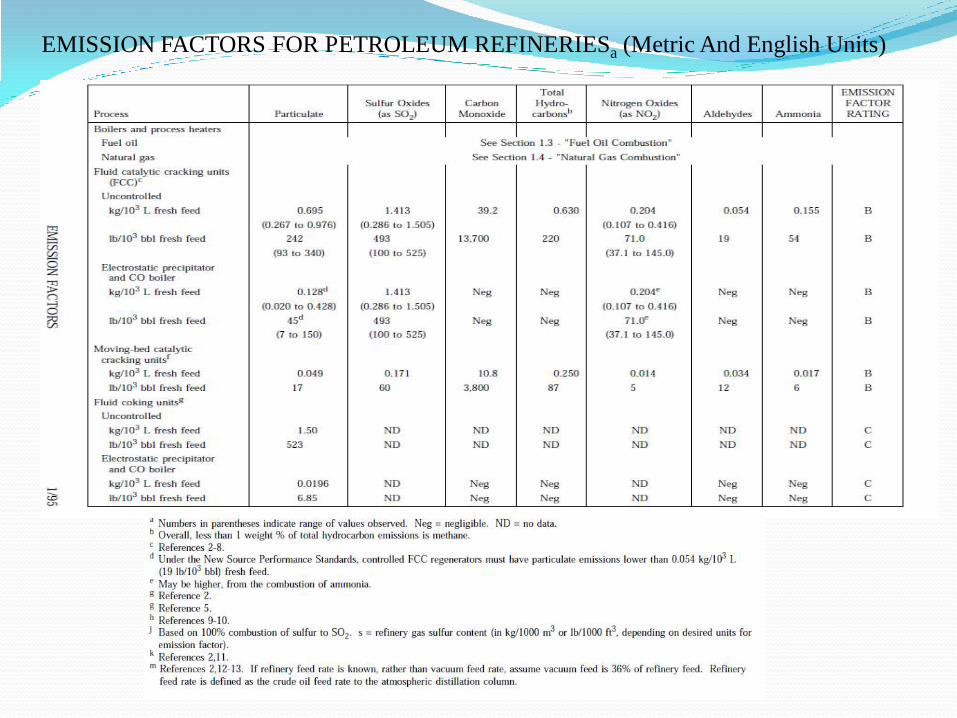
EMISSION FACTORS FOR PETROLEUM REFINERIESa (Metric And English Units)

Air-Quality Modeling

Ambient air-quality monitoring is an expensive undertaking; even large cities

may have only a relatively few monitoring stations. Air-quality models provide

a relatively inexpensive means of predicting the degree of emission reduction

necessary to attain ambient air-quality standards.

The object of a model is to determine mathematically the effect of source

emissions on ground-level concentrations, and to establish that permissible

levels are not being exceeded.

Models have been developed for a variety of pollutants and time

circumstances. Although the use of air-quality models is a subject of some

controversy, there is a general agreement that there are few alternatives to their

use, particularly in making decisions on an action which is known in advance

to pose a potential environmental problem.

The debate arises as to which models should be used and the interpretation of

model results. The underlying question in such debates is how well, or how

accurately, does the model predict concentrations under the specific

circumstances.

Meteorological Aspects of Air Pollutant Dispersion

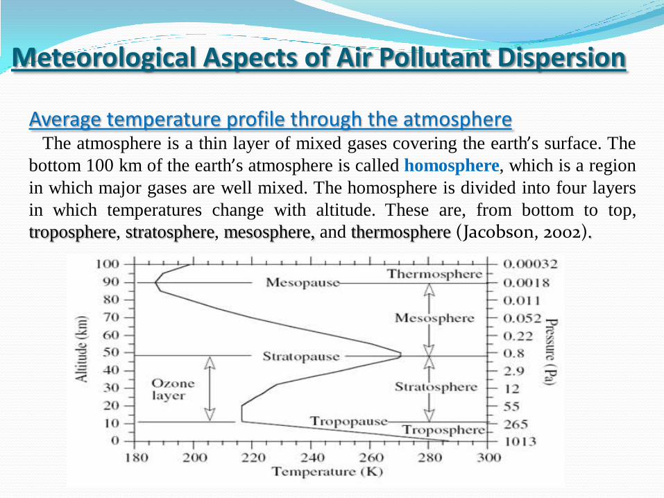
Average temperature profile through the atmosphere The atmosphere is a thin layer of mixed gases covering the earth’s surface. The

bottom 100 km of the earth’s atmosphere is called homosphere, which is a region

in which major gases are well mixed. The homosphere is divided into four layers

in which temperatures change with altitude. These are, from bottom to top,

troposphere, stratosphere, mesosphere, and thermosphere (Jacobson, 2002).

The troposphere is extending in altitude from the earth’s surface to

approximately 11 kilometers. The temperature of the troposphere ranges from

an average of 15°C at sea level to an average of -56°C at its upper boundary; it

is dividing into:

•The boundary layer

• The free troposphere (geostrophic layer or layer of frictionless velocity).

The boundary layer (planitery boundary layer, PBL) extends from the

surface to the altitude between 500 and 3000 m. All Human live in the

boundary layer, so it is this region of the atmosphere in which pollution

buildup is of the most concern. Pollutants are emitted near the ground

accumulate in this layer. When these pollutants escape from the boundary

layer, they can travel horizontally long distances before they are removed

from the air.

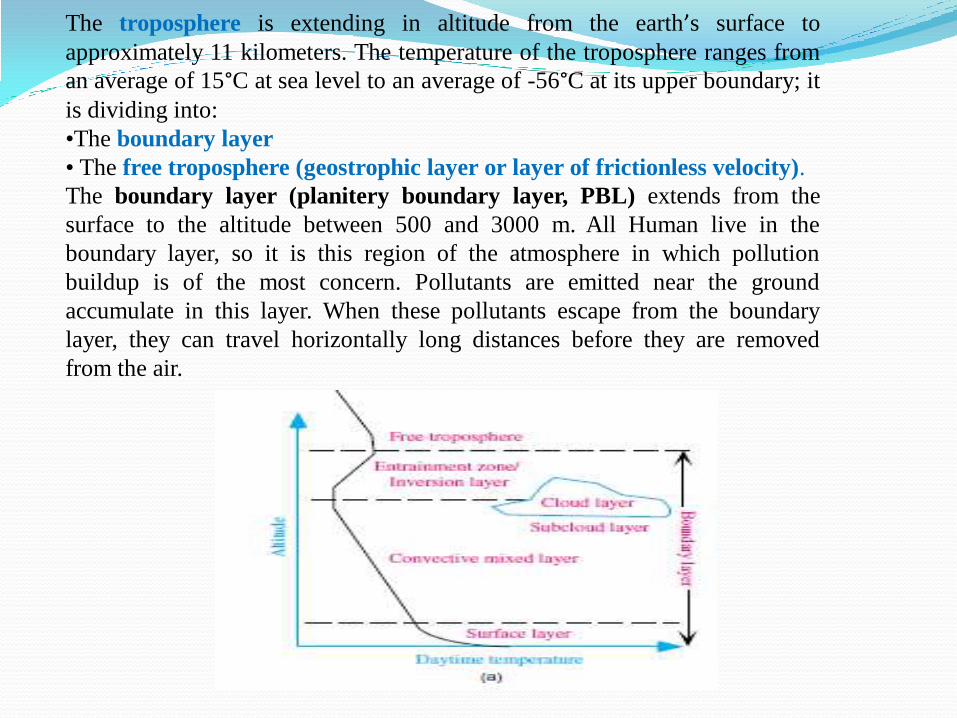
The bellow figure shows a typical temperature variation in the boundary

layer over land during the day and night. During the day, the boundary layer

is characterized by a surface layer, a convective mixed layer, and an

inversion layer (Jacobson, 2002). The pollutants released at ground level will be mixed almost uniformly up

to the mixing height but not above it, thus the mixing height sets the upper

limit to dispersion of atmospheric pollutants.

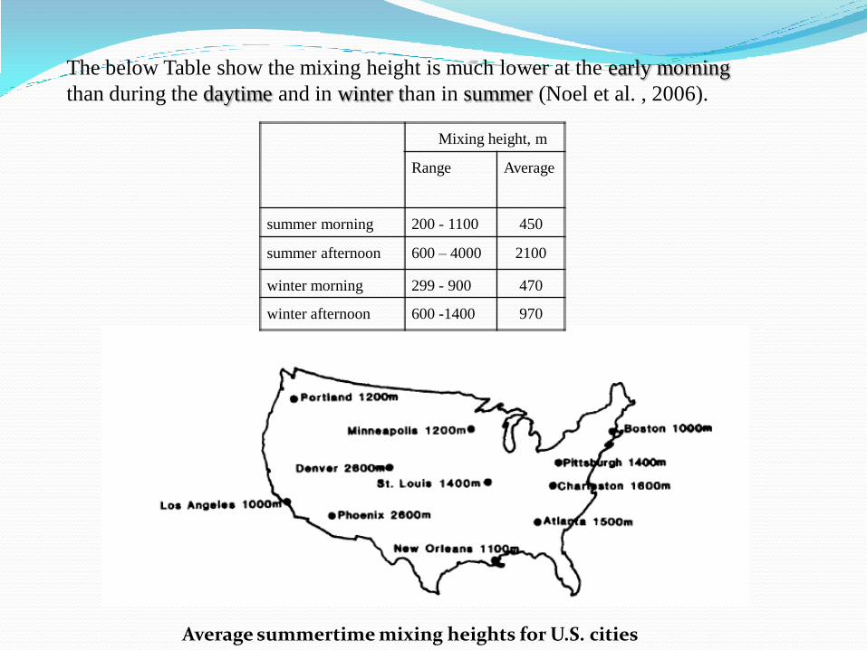
The below Table show the mixing height is much lower at the early morning

than during the daytime and in winter than in summer (Noel et al. , 2006).

Average summertime mixing heights for U.S. cities

Mixing height, m

Range

Average

summer morning 200 - 1100 450

summer afternoon 600 – 4000 2100

winter morning 299 - 900 470

winter afternoon 600 -1400 970

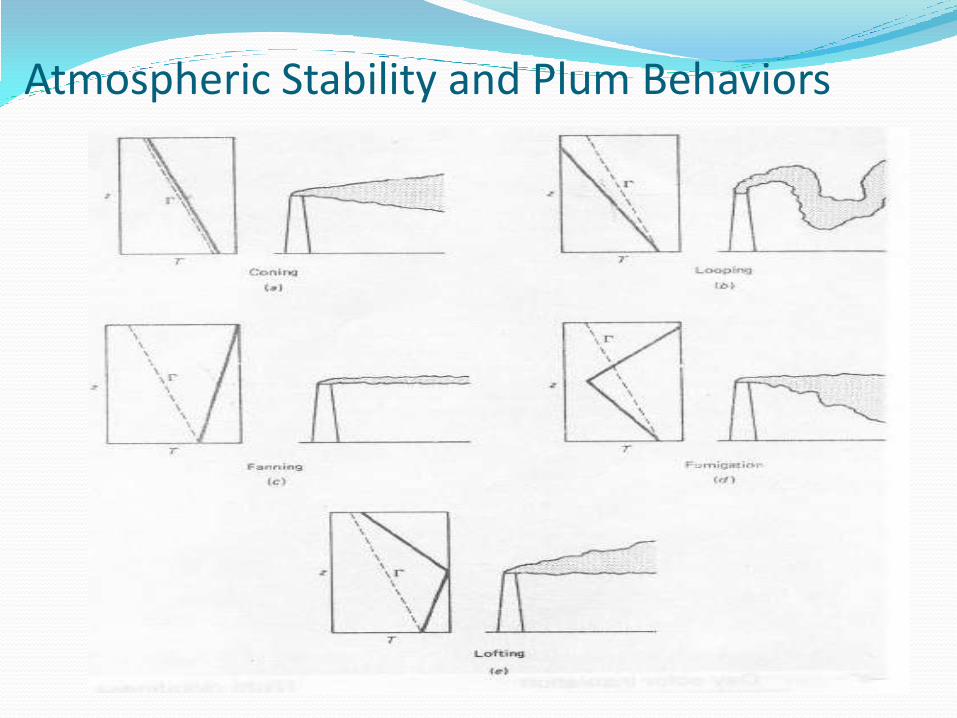
Atmospheric Stability and Plume Behaviors

One of the most important characteristics of the atmosphere is

its stability that is tendency to resist vertical motion or to

suppress existing turbulence.

The degree of stability of the atmosphere is determined by the

temperature difference between an air parcel and the air

surrounding it. This difference can cause the parcel to move

vertically (i.e., it may rise or fall).

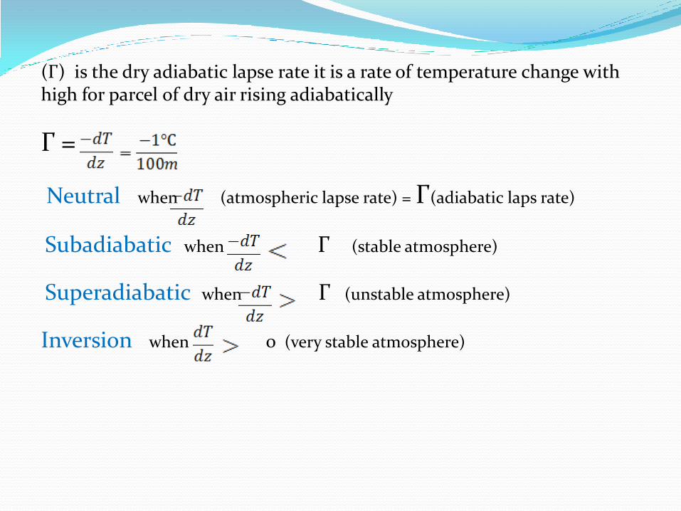
(Γ) is the dry adiabatic lapse rate it is a rate of temperature change with high for parcel of dry air rising adiabatically

Γ =

Neutral when (atmospheric lapse rate) = Γ(adiabatic laps rate)

Subadiabatic when Γ (stable atmosphere)

Superadiabatic when Γ (unstable atmosphere)

Inversion when 0 (very stable atmosphere)

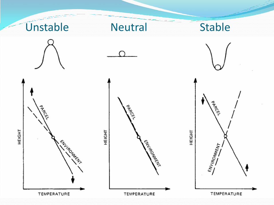
Unstable Neutral Stable

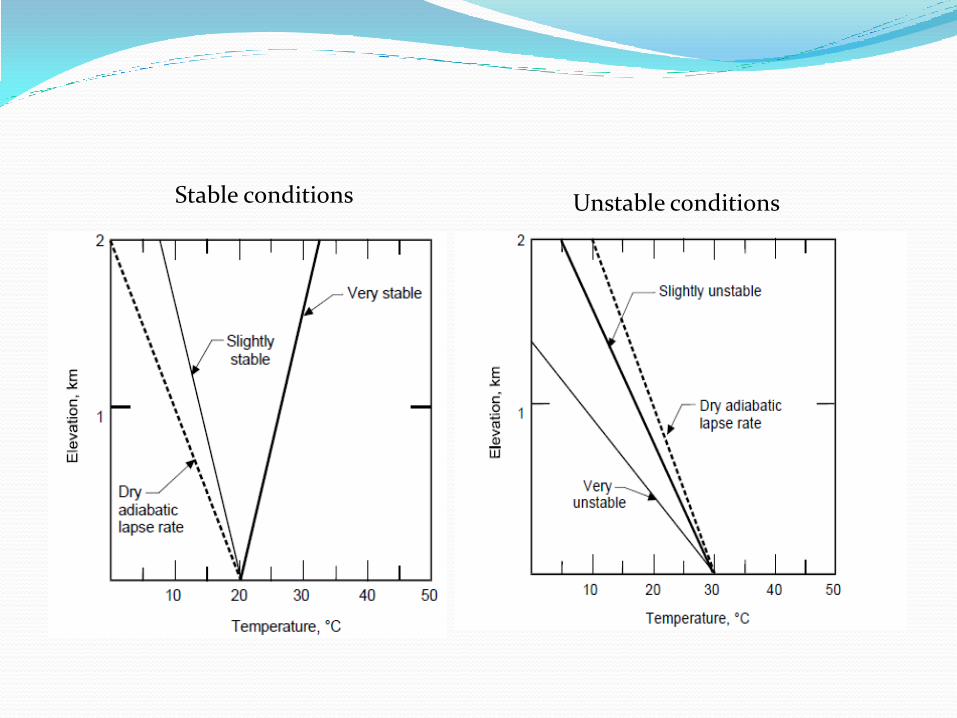
Stable conditions Unstable conditions

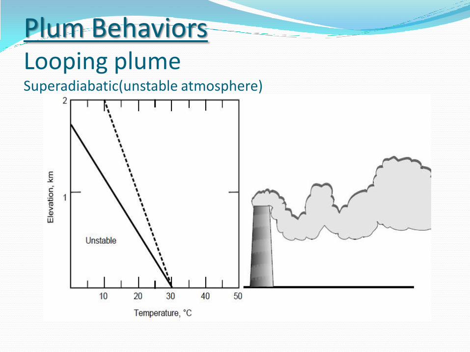
Plum Behaviors Looping plume Superadiabatic(unstable atmosphere)

Fanning plume

Inversion(very stable atmosphere)

Coning plume neutral (stable atmospher)

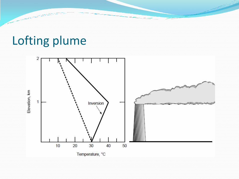
Lofting plume

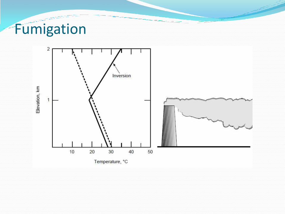
Fumigation

Atmospheric Stability and Plum Behaviors

Topographic Effects(Terrain Effect) Surface topography can modify the general

pattern of wind speed and direction, many cases

can be observed:

Land and sea breeze

Mountain and valley wind system

Heat island

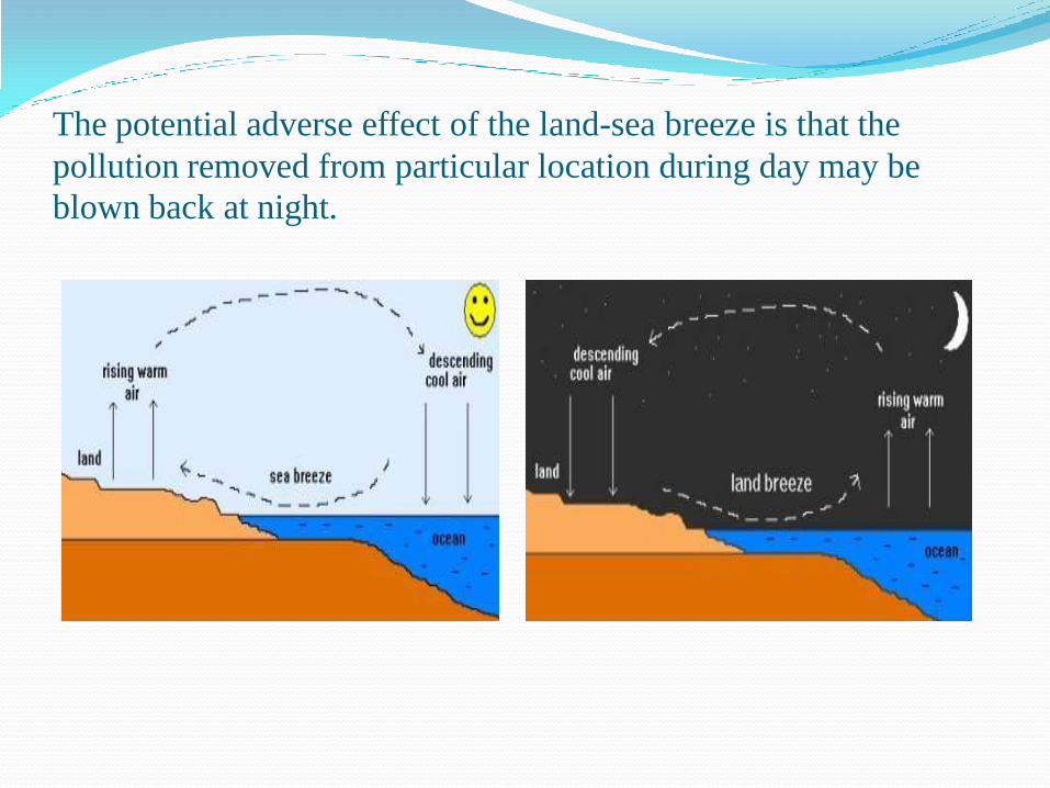
The potential adverse effect of the land-sea breeze is that the

pollution removed from particular location during day may be

blown back at night.

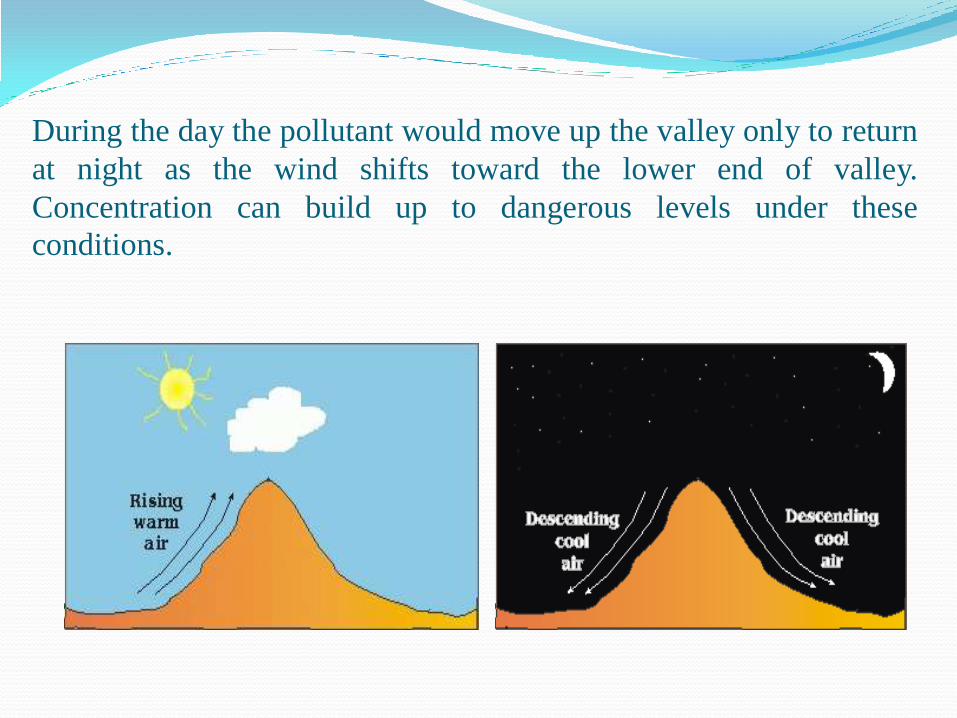
During the day the pollutant would move up the valley only to return

at night as the wind shifts toward the lower end of valley.

Concentration can build up to dangerous levels under these

conditions.

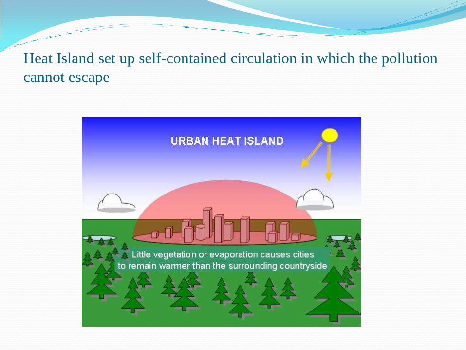
Heat Island set up self-contained circulation in which the pollution

cannot escape

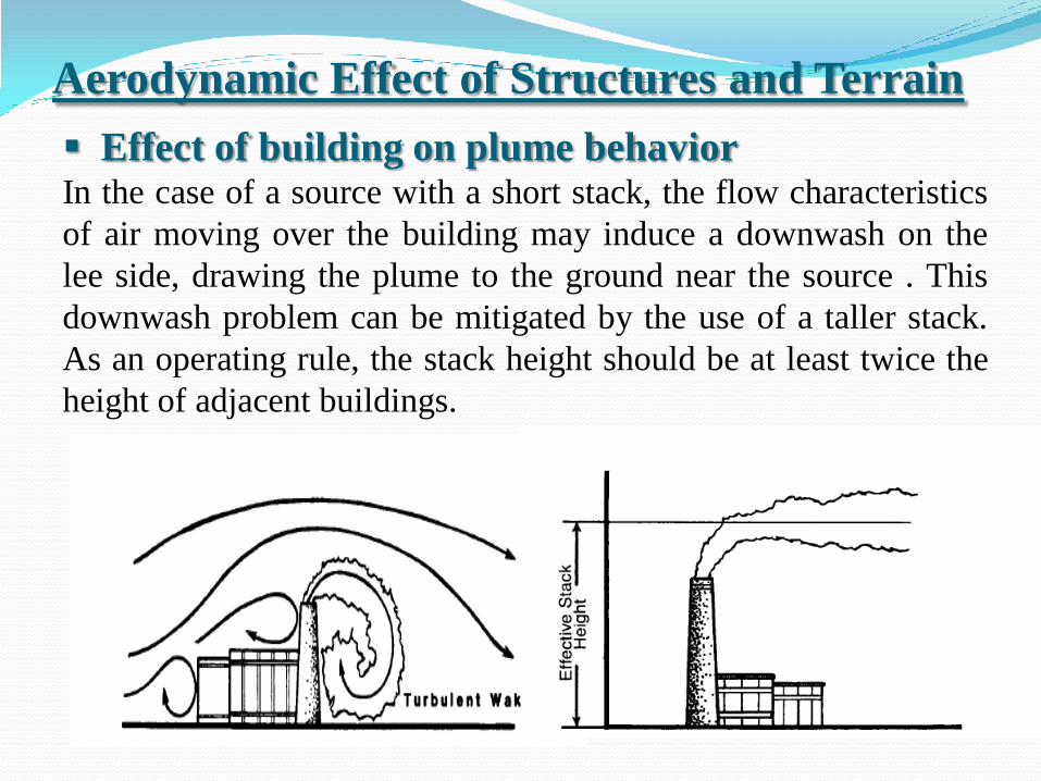
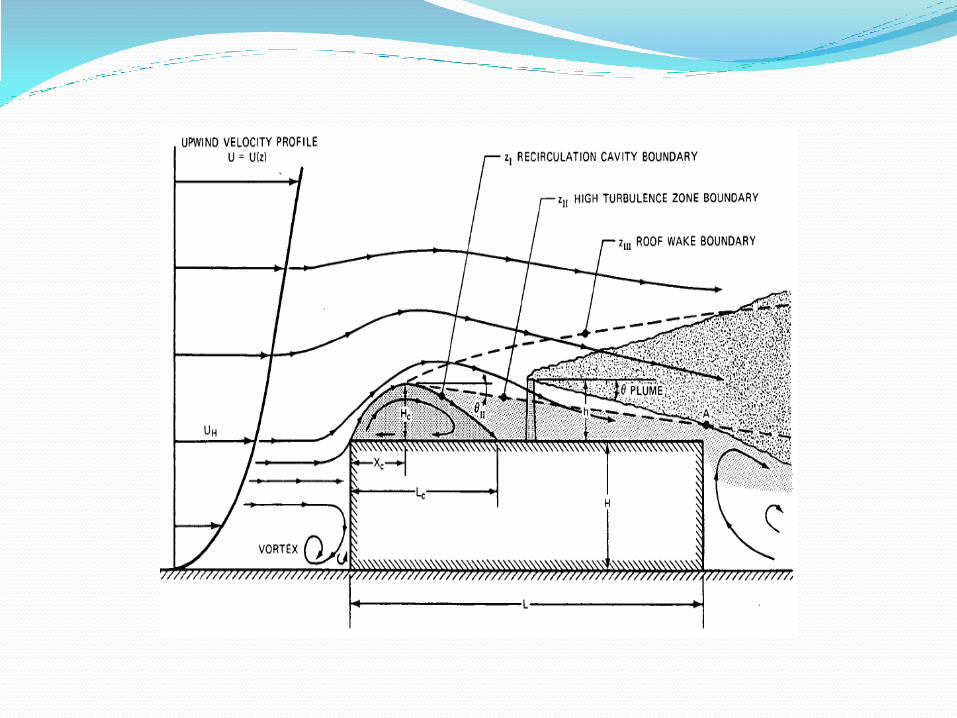
Aerodynamic Effect of Structures and Terrain Effect of building on plume behavior In the case of a source with a short stack, the flow characteristics

of air moving over the building may induce a downwash on the

lee side, drawing the plume to the ground near the source . This

downwash problem can be mitigated by the use of a taller stack.

As an operating rule, the stack height should be at least twice the

height of adjacent buildings.

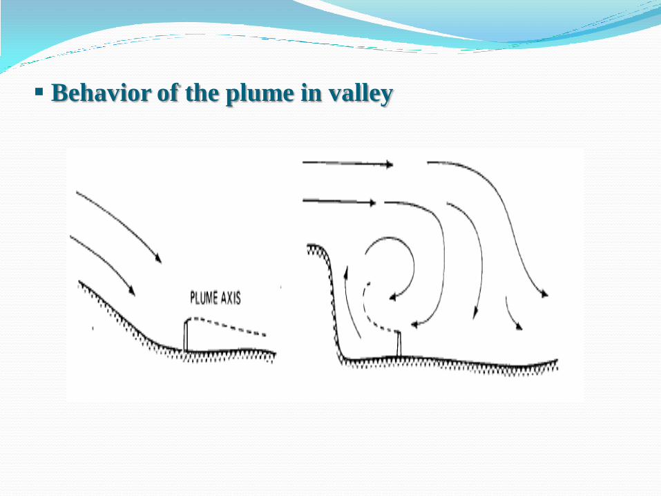
Behavior of the plume in valley

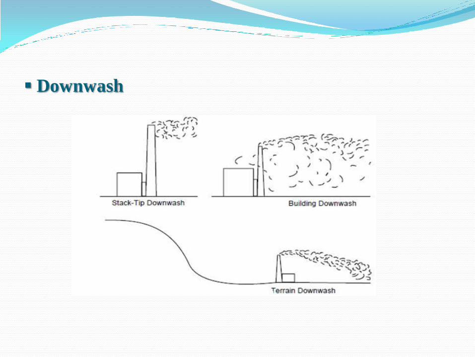
Downwash

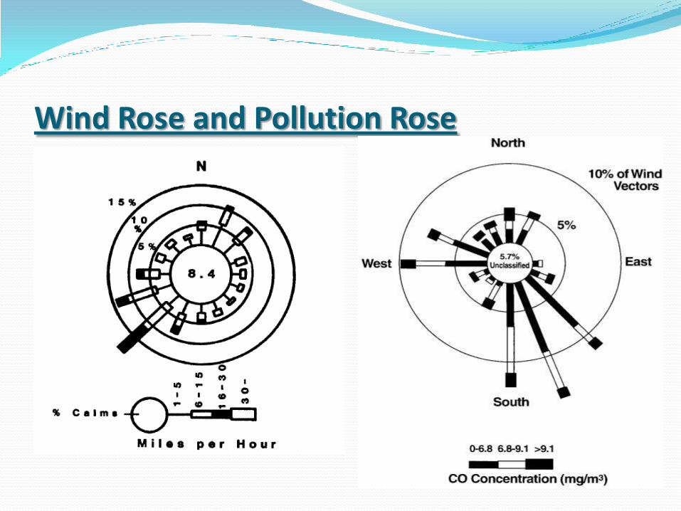
Wind Rose and Pollution Rose

Dispersion of Air Pollutants There are several models available to predict the concentration

downwind from a source: Short-term models are used to calculate concentrations of

pollutants over a few hours or days. They require detailed

understanding of chemical reactions and atmospheric processes on

the order of minutes to hours. Such models can be employed to

predict worst case episode conditions and are often used by

regulatory agencies as a basis for control strategies.

Long-term models are designed to predict seasonal or annual

average concentrations, which may prove useful in studying

potential health effects.

Nonreactive models are applied to pollutants such as CO and

SO2.

Reactive models are applied for photochemical pollutant such as

O3.

Advanced models have been developed for such problems as

photochemical pollution, dispersion in complex terrain, long-range

transport, and point sources over uneven terrain.

The most widely used models for predicting the impact of

relatively uncreative gases, released from smokestacks are based

on Gaussian diffusion.

In Gaussian plume models, it is assumed that concentrations of

pollutants associated with a continuously emitting plume are

proportional to the emission rate and inversely proportional to

wind speed. It is also assumed that, as a result of molecular

diffusion pollutant concentrations in the horizontal and vertical

dimensions of a plume will be normally distributed. These

models assume that pollutants do not undergo significant

chemical reaction or removal as they travel away from a source,

and as the plume grows vertically it is evenly reflected back

toward the plume centerline.

Point Source Emission at Ground Level

u = average wind velocity, m/s C = concentration, µg/m3

Q = emission rate, µg/s

= standard deviation in z direction, m

= standard deviation in y direction, m

Gaussian distribution

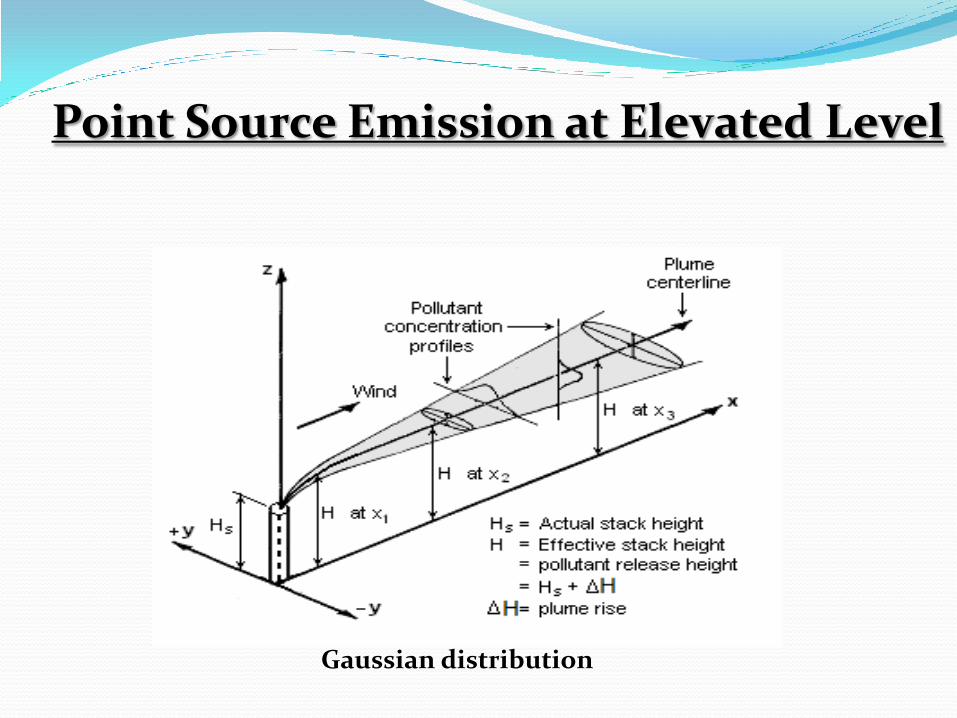
Point Source Emission at Elevated Level

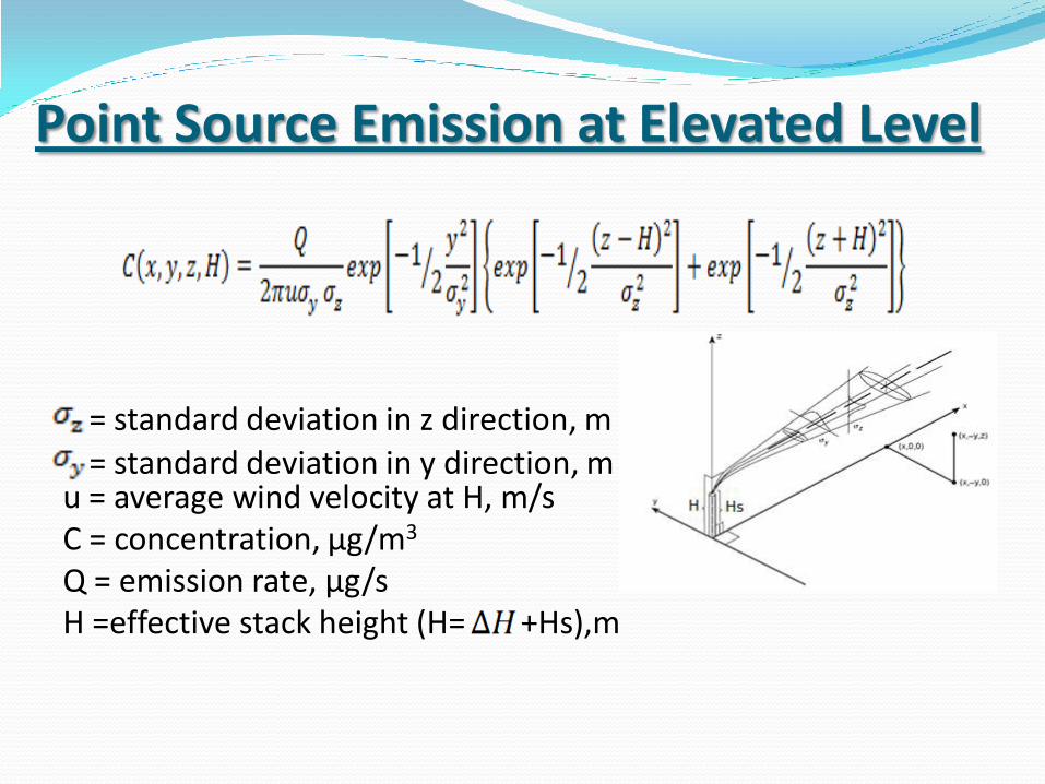
Point Source Emission at Elevated Level

u = average wind velocity at H, m/s C = concentration, µg/m3

Q = emission rate, µg/s H =effective stack height (H= +Hs),m

= standard deviation in y direction, m

= standard deviation in z direction, m

Concentration at ground level

Concentration at center line

Maximum concentration ( )

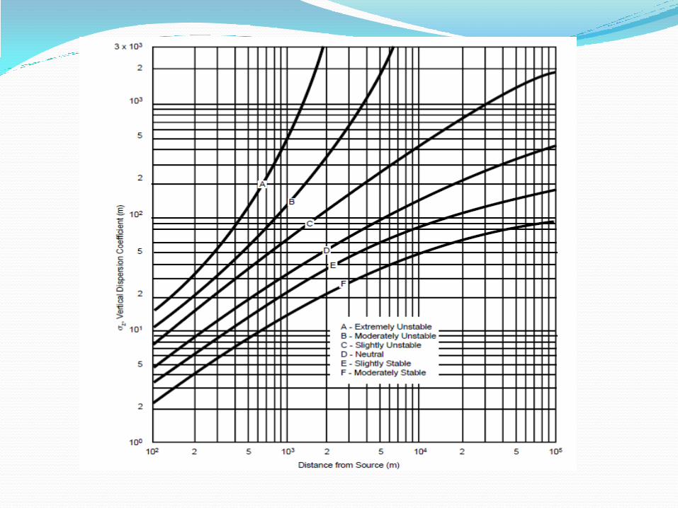
Stability Classes for Determining Dispersion Coefficients

Pasquill’s dispersion coefficients . (From Turner, D.B. 1969.workbook or Atmospheric Dispersion

Estimates.EPA Publication No. AP-26.)

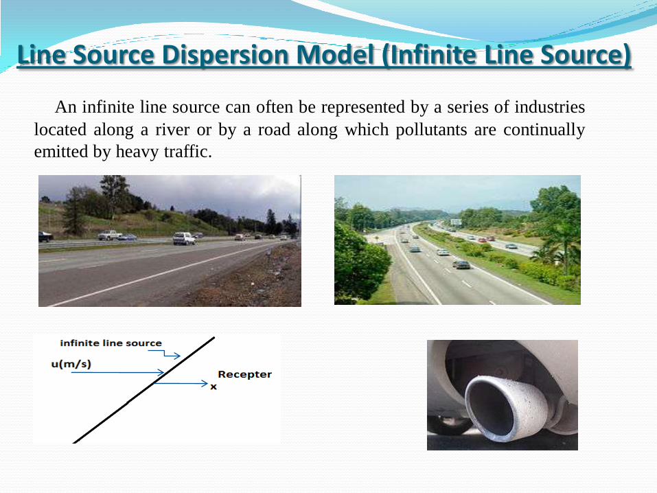
Line Source Dispersion Model (Infinite Line Source)

An infinite line source can often be represented by a series of industries

located along a river or by a road along which pollutants are continually

emitted by heavy traffic.

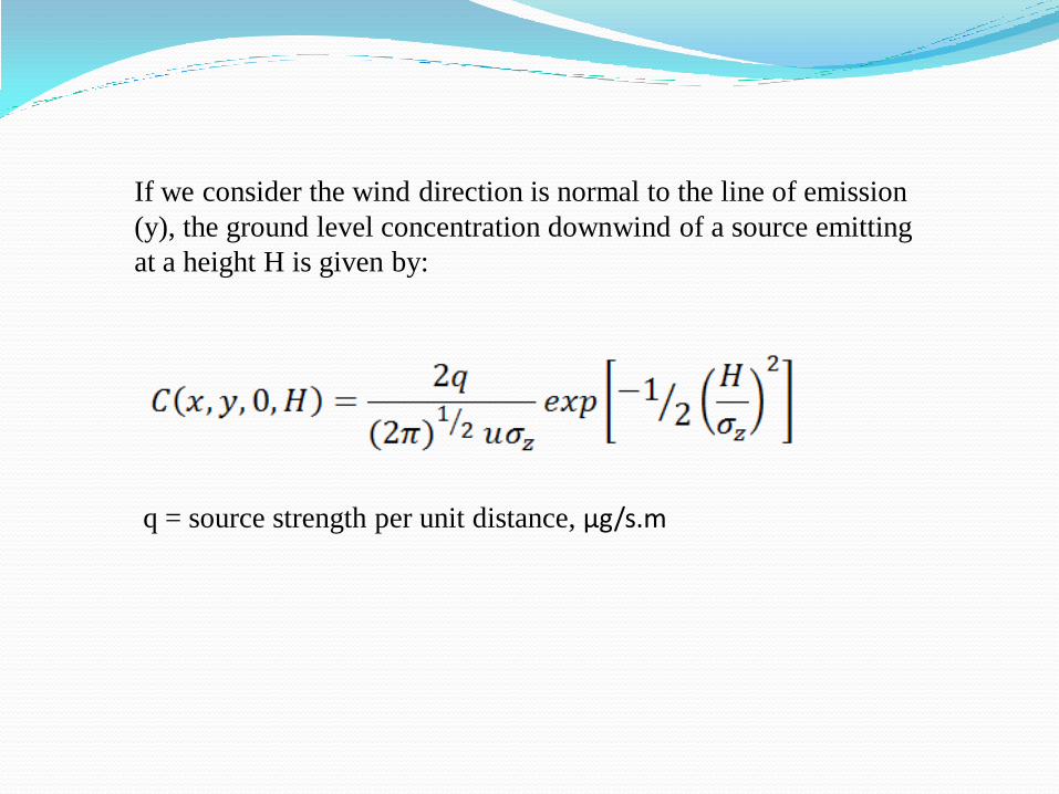
q = source strength per unit distance, µg/s.m

If we consider the wind direction is normal to the line of emission

(y), the ground level concentration downwind of a source emitting

at a height H is given by:

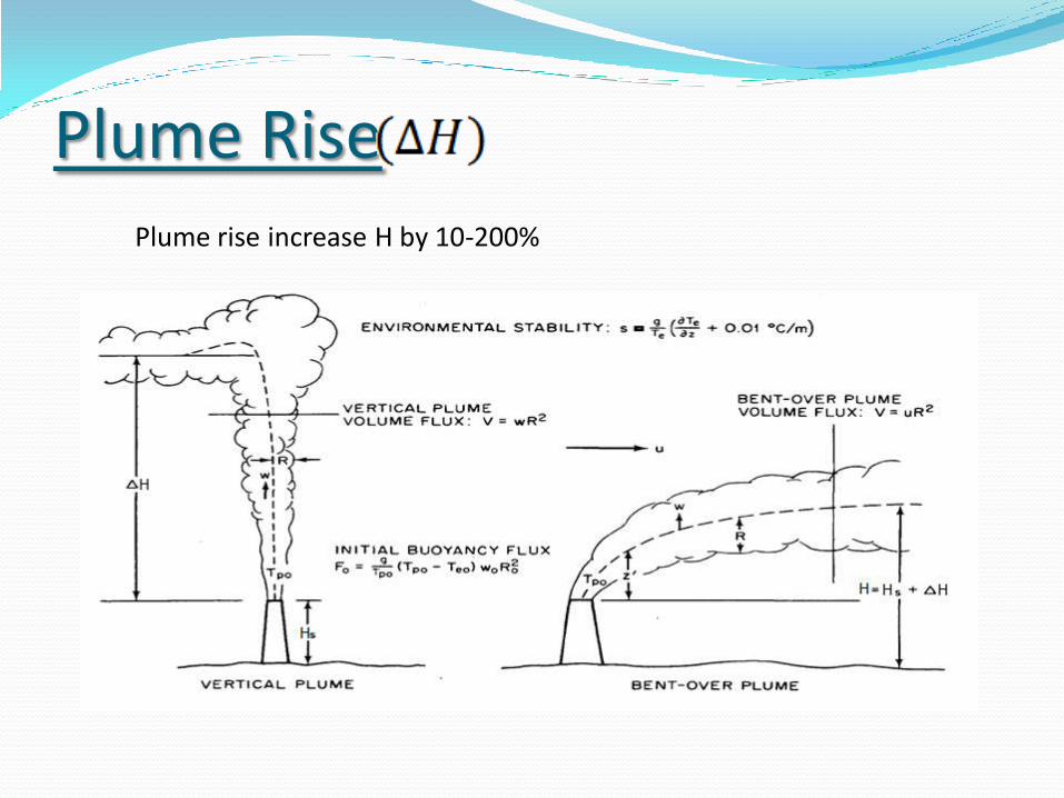
Plume Rise Plume rise increase H by 10-200%

Briggs Formula For unstable (A,B,C) and neutral (D)conditions,when

Downwind distance to final plume rise

u = wind speed at stack tip m/s

F = buoyancy flux parameter m4/s3

for m

for m

vs= stack exit velocity/s

rs= stack tip radius ,m

Ts= stack temperature, K

Ta = air temperature, K

For

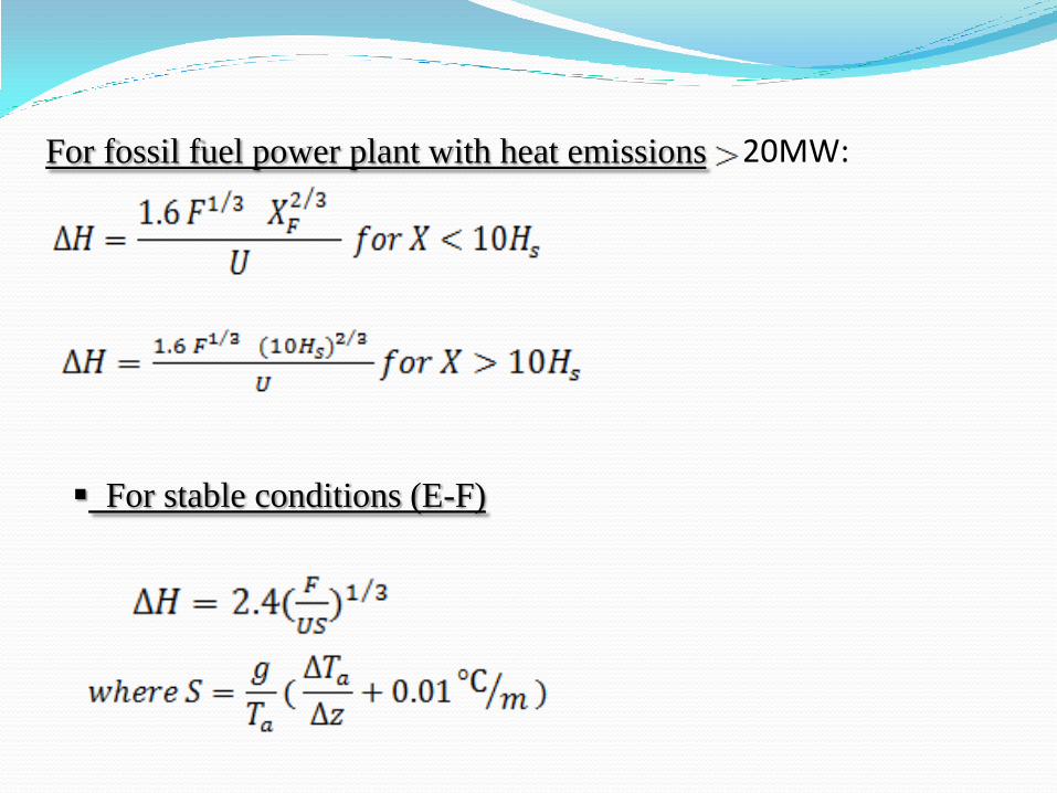
For fossil fuel power plant with heat emissions 20MW:

For stable conditions (E-F)

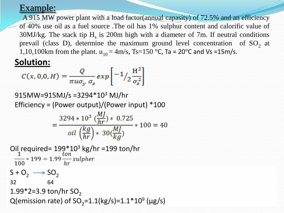
Example: A 915 MW power plant with a load factor(annual capasity) of 72.5% and an efficiency

of 40% use oil as a fuel source .The oil has 1% sulphur content and calorific value of

30MJ/kg. The stack tip Hs is 200m high with a diameter of 7m. If neutral conditions

prevail (class D), determine the maximum ground level concentration of SO2 at

1,10,100km from the plant. u10 = 4m/s, Ts=150 °C, Ta = 20°C and Vs =15m/s.

Solution: 915MW=915MJ/s =3294*103 MJ/hr Efficiency = (Power output)/(Power input) *100

Oil required= 199*103 kg/hr =199 ton/hr

S + O2 SO2

32 64

1.99*2=3.9 ton/hr SO2

Q(emission rate) of SO2=1.1(kg/s)=1.1*109 (µg/s)

Estimation of

using Briggs equation for neutral conditions, then:

For X=1000m

For x =10000m and 100000m

Using the below equation to estimate the concentration:

,

Estimate u at effective stack height using power low

# Calculate the concentration at x=10000 and 100000m

EPA Computer Programs for Regulation of Industry

The industrial source complex model

One of the most widely used models for estimating concentrations of non reacting

pollutants within a 10 mile radius of the source is EPA’s Industrial Source Complex Short-

Term, Version 3 (ISCST3) program. The short- term program includes 1, 2, 3, 4, 6, 8, 12,

and 24 hr. It is a steady-state Gaussian plume model. Therefore, the parameters such as

meteorological conditions and emission rate are constant throughout the calculation. There

is also a long-term program, ISCLT.

Screening models If there are few sources or emissions which are not very large, it is usually advantageous to employ a screening model .SCREEN3 allows a group of sources to be merged into one source, and it can account for elevated terrain, building downwash, and wind speed modifications for turbulence. The new models CALPUFF, a multilayer, multispecies, non steady-state dispersion model that views a plume as a series of puffs is a new model under consideration. This model simulates space–time, varying meteorological conditions on pollutant–transport, chemical reaction, and removal. It can be applied from around 100 ft downwind up to several hundreds of miles. The American Meteorological Society/EPA Regulatory Model (AERMOD) is a refined model currently under development by EPA as a supplement to ISCST3 for regulatory purposes.

Thank you