AIR POLLUTION – Nature and Origin of PM and Smaller ... · Environmental RTDI Programme...
116
Environmental RTDI Programme 2000–2006 AIR POLLUTION – Nature and Origin of PM 10 and Smaller Particulate Matter in Urban Air (2000-LS-6.1-M1) Final Report Prepared for the Environmental Protection Agency by Atmospheric Research Group, Department of Experimental Physics, National University of Ireland, Galway Authors: S.G. Jennings, D. Ceburnis, A.G. Allen, J. Yin, R.M. Harrison, M. Fitzpatrick, E. Wright, J. Wenger, J. Moriarty, J.R. Sodeau and E. Barry ENVIRONMENTAL PROTECTION AGENCY An Ghníomhaireacht um Chaomhnú Comhshaoil PO Box 3000, Johnstown Castle, Co. Wexford, Ireland Telephone: +353 53 916 0600 Fax: +353 53 916 0699 E-mail: [email protected] Website: www.epa.ie
Transcript of AIR POLLUTION – Nature and Origin of PM and Smaller ... · Environmental RTDI Programme...
Environmental RTDI Programme 2000–2006
AIR POLLUTION – Nature and Origin of PM10
and Smaller Particulate Matter in Urban Air
(2000-LS-6.1-M1)
Final Report
Prepared for the Environmental Protection Agency
by
Atmospheric Research Group, Department of Experimental Physics,
National University of Ireland, Galway
Authors:
S.G. Jennings, D. Ceburnis, A.G. Allen, J. Yin, R.M. Harrison, M. Fitzpatrick, E. Wright,
J. Wenger, J. Moriarty, J.R. Sodeau and E. Barry
ENVIRONMENTAL PROTECTION AGENCY
An Ghníomhaireacht um Chaomhnú ComhshaoilPO Box 3000, Johnstown Castle, Co. Wexford, Ireland
Telephone: +353 53 916 0600 Fax: +353 53 916 0699E-mail: [email protected] Website: www.epa.ie

mme isred onental
arch.
lication,uthor(s)ioned, in mattersion,
© Environmental Protection Agency 2006
ACKNOWLEDGEMENTS
This report has been prepared as part of the Environmental Research Technological Development andInnovation Programme under the Productive Sector Operational Programme 2000–2006. The prografinanced by the Irish Government under the National Development Plan 2000–2006. It is administebehalf of the Department of the Environment, Heritage and Local Government by the EnvironmProtection Agency which has the statutory function of co-ordinating and promoting environmental rese
DISCLAIMER
Although every effort has been made to ensure the accuracy of the material contained in this pubcomplete accuracy cannot be guaranteed. Neither the Environmental Protection Agency nor the aaccept any responsibility whatsoever for loss or damage occasioned or claimed to have been occaspart or in full, as a consequence of any person acting, or refraining from acting, as a result of acontained in this publication. All or part of this publication may be reproduced without further permisprovided the source is acknowledged.
ENVIRONMENTAL RTDI PROGRAMME 2000–2006
Published by the Environmental Protection Agency, Ireland
PRINTED ON RECYCLED PAPER
ISBN: 1-84095-191-5
Price: €25 11/06/300
ii

Details of Project Partners
S.G. JenningsAtmospheric Research GroupDepartment of Experimental Physics/Environmental Change InstituteNational University of Ireland, GalwayGalwayIreland
Tel.: +353 91 492490Fax: +353 91 494584E-mail: [email protected]
D. CeburnisAtmospheric Research GroupDepartment of Experimental Physics/Environmental Change InstituteNational University of Ireland, GalwayGalwayIreland
A.G. AllenDivision of Environmental Health & Risk ManagementSchool of Geography, Earth & Environmental SciencesUniversity of BirminghamUK
J. YinDivision of Environmental Health & Risk ManagementSchool of Geography, Earth & Environmental SciencesUniversity of BirminghamUK
R.M. HarrisonDivision of Environmental Health & Risk ManagementSchool of Geography, Earth & Environmental SciencesUniversity of BirminghamUK
M. FitzpatrickAtmospheric and Noise UnitCommunity and Environment DepartmentDublin City CouncilDublinIreland
E. WrightAtmospheric and Noise UnitCommunity and Environment DepartmentDublin City CouncilDublinIreland
J. WengerDepartment of ChemistryEnvironmental Research InstituteUniversity College CorkCorkIreland
J. MoriartyDepartment of ChemistryEnvironmental Research InstituteUniversity College CorkCorkIreland
J.R. SodeauDepartment of ChemistryEnvironmental Research InstituteUniversity College CorkCorkIreland
E. BarryEnvironmental LaboratoryCork City CouncilCorkIreland
iii


Table of Contents
Acknowledgements ii
Disclaimer ii
Details of Project Partners iii
Summary vii
1 Introduction 1
2 Measurement Methodologies 3
2.1 Aerosol Sampling 3
2.1.1 Sampling locations 3
2.1.2 Aerosol sampling 4
2.2 Analytical Methods 5
2.2.1 Gravimetric analysis of PM10 and PM2.5 masses 5
2.2.2 Chemical analyses for ionic species 5
2.2.3 Determination of carbonaceous compounds 5
2.2.4 Chemical analysis for PAHs 6
2.2.5 Chemical analysis for metals 6
3 Overview of Concentration Levels of PM10 and PM2.5 Masses and their Chemical Components in the Irish Atmosphere 8
3.1 Atmospheric Concentrations of Particle Mass 8
3.1.1 Long-term and short-term variation of PM mass concentrations 8
3.1.2 Number of exceedances of the PM10 standard limit 11
3.2 Atmospheric Concentrations of Particle Chemical Components 11
3.3 Relationship between Monthly PM Mass and its Major Chemical Component Concentrations 14
4 Measurements over an Intensive Period 25
4.1 Local Meteorology during the Intensive Campaign 25
4.2 Gaseous Measurements and Condensation Particle Counts during the Intensive Campaign 26
4.3 Size-Resolved Particle Distribution, Obtained by MOUDI Impactors, and Chemical Composition during the Intensive Campaign 29
v
76
6
5 PM10 Episodes Study and Air Mass Back-Trajectory Analyses 37
5.1 Relative Importance of Fine and Coarse Particles and their Chemical Composition during PM10 Episodes 37
5.2 Use of Air Mass Back Trajectories in Analysis of PM10 Episodes 37
5.3 Mean Concentration Estimates for PM Mass and Chemical Components for Different Air Mass Origins 45
6 Source Apportionment of Aerosol PM10, PM2.5 and PM2.5–10 55
6.1 PM Source Apportionment Using the Chemical Reconstruction Method 55
6.1.1 Mass closure analysis using measured chemical components 55
6.1.2 Mass closure analysis using reconstructed chemical components 55
6.2 PM Source Apportionment Using a Statistical Modelling Approach 58
6.2.1 Factor analysis 59
6.2.2 MLR analysis 60
6.3 Comparison between Modelled and Reconstructed Component Mass 70
6.4 Results of the Revised Chemical Reconstruction 71
7 Metals 75
7.1 Sources of Trace Metals 75
7.2 Monthly Variation in Metal Concentration 76
7.3 Seasonal Trends in Trace Metal Concentrations during July 2001–December 2002
7.4 Summary 88
7.4.1 Coarse fraction 88
7.4.2 Fine fraction 89
8 Polycyclic Aromatic Hydrocarbons (PAHs) 90
8.1 Sources of PAHs 90
8.2 Monthly Variation in Concentration of PAHs 90
8.3 Trends in PAH Concentration 92
8.4 Summary 93
9 General Conclusions and Recommendations for Future Work 105
9.1 General Conclusions 105
9.2 Recommendations for Future Work 10
10 References 107
vi

Summary
The major source categories contributing to particulate air
pollution in urban as well as non-urban areas of Ireland
were studied over an 18-month period (July 2001 to
December 2002) using measurements at five sites
including urban roadside (Site A), urban
centre/background (Sites B and E), rural (Site D) and
coastal (Site C) environments. Daily fine and coarse
aerosol samples were collected at each site using
dichotomous Partisol samplers. The measurements
included gravimetric mass (PM10, PM2.5 and PM2.5–10),
soluble ions (SO42–, NO3
–, Cl–, CH3SO3–, NH4
+, Na+, K+,
Mg2+ and Ca2+), elemental carbon (EC) and organic
carbon (OC). Measurements of polycyclic aromatic
hydrocarbon (PAH) content as well as trace metal
concentration of samples were also carried out. In
addition, more intensive measurements were carried out
over a 4-week period at three of the sites (rural, city centre
and coastal), which included size-resolved (12 size
categories) impactor sampling as well as condensation
particle count (CPC) and SO2, NO, NO2, NOx, O3 and CO
gaseous measurements.
An annual averaged PM10 mass of 35.4 µg/m3 for 2002
was a maximum at the Dublin city kerbside site, with
values of 22–24 µg/m3 for the Dublin and Cork city centre
sites. Corresponding PM2.5 mass concentration values
were 21.5 µg/m3 and 11.5–12.5 µg/m3, respectively. The
coastal site had averaged annual values for PM10 and
PM2.5 mass concentration of 20 µg/m3 and 12.5 µg/m3,
while the rural background site had values of 10.5 and 6.3
µg/m3, respectively.
Mass closure procedures using reconstructed chemical
components were used to identify major source
categories contributing to the aerosol mass, namely
primary marine aerosol (NaCl), secondary inorganic
materials (NH4NO3 + (NH4)2SO4), primary anthropogenic
combustion materials (EC), primary and secondary
organic materials, and resuspended dusts. Source
component contributions differed for fine and coarse
particles and at different locations. In urban areas, the
major components contributing to fine particle mass
(together accounting for 79–84% of PM2.5 mass) were, in
order, organic compounds, EC, ammonium
sulphate/ammonium nitrate, whilst in the coarse fraction
resuspended material and sea salt were predominant
(56–66%). At the rural and coastal sites, PM2.5 mainly
consisted of ammonium sulphate/ammonium nitrate and
organic materials (65%), whilst sea salt was the largest
contributor to coarse particles (39% rural, 56% coastal).
Unexplained materials, accounting for about 7–28% of the
mass, were attributed mainly to resuspended materials at
urban sites and organic materials at the other sites, as
well as unmeasured water content.
Chemical component analysis (for secondary aerosol
components of sulphate, nitrate and ammonium),
according to air mass origin from data in Chapter 5,
indicates that long-range transport from an easterly
direction – mainly from the continent and the UK – to
Dublin City (Site B) accounts for up to about 30% of the
PM2.5 mass (as a fraction of the total mass) over and
above that obtained under westerly or maritime air mass
conditions, and about 25% of PM10 mass. Results also
show that local sources account for at least 50% of PM2.5
and of PM10 mass for the city centre sites.
The levels of PAHs were largest at the Dublin roadside
(Site A), whilst similar concentrations were observed at
the urban background sites in Dublin (B) and Cork (E) due
to the large number of combustion sources. Very low
concentrations of the PAHs were observed at the coastal
and rural sites due to the lack of significant sources. The
concentrations of the particle-phase PAHs measured at
the five sites are similar to those observed at other
locations around the world. The concentration of
benzo(a)pyrene is of particular interest because a
threshold value of 1 ng/m3 will be introduced as part of a
new EU directive. The average monthly concentration
exceeded the threshold value on a number of occasions
at all urban sites. This EU Directive 2004/107/EC of the
European Parliament and Council of 15 December 2004
relates to arsenic, cadmium, mercury, nickel and PAHs in
ambient air and it sets a target for PAHs (using B(a)P as
a marker) of 1.0 ng/m3 to be achieved by 31 December
2012.
The highest concentrations for all metals, except
magnesium, were detected at the kerbside city centre site
(Site A). This was expected, mainly due to the large
vii

S.G. Jennings et al., 2000-LS-6.1-M1
number of vehicles passing the site. Within the urban
sites, Site A had the highest concentration of the crustal
elements Ca and Fe. Average Ca levels in Site B were
almost equal to those at Site A. The concentrations at
these Dublin sites were almost double those observed in
Site E (Cork). This difference could be due to higher
amounts of resuspended road dust in the Dublin sites,
probably due to the higher volumes of traffic.
The Ca concentrations at Sites C, D and E were quite
similar, with higher values for the urban sit (Site E). Fe
concentrations are highest at Site A, with Sites B and E
possessing higher levels than the rural and coastal sites.
Since Fe is associated with vehicle emissions, then these
results are not surprising. Site A showed higher
concentrations for the toxic trace metals (Mn, Pb, Cd, Zn,
Ni, Cr, V and Cu) than either of the other urban sites. In
general, the rural site (Site D, Co. Galway) showed the
lowest level of all metals. This was to be expected as this
site was removed from any direct vehicle emissions and
had no industry within the vicinity. The coastal site
showed the highest concentration of magnesium in the
coarse fraction in comparison to all other sites. Normally
there are high levels of magnesium in sea spray so these
observations are consistent with other results.
As with the coarse fraction, the higher concentrations of
trace metals in the fine fraction were usually observed at
Site A. Within the urban sites (A, B and E), Site A had
consistently higher concentrations than B and E, except
for Ni (highest at Site B). Sites B and E showed similar
concentrations for all metals in this fraction. This was
expected since B and E are both urban background sites.
The coastal (C) and rural (D) sites generally showed lower
fine fraction concentrations of the metals than the urban
sites.
Intensive measurements were carried out during four
weeks in February–March 2002 (19 February–21 March)
at three sites: the rural (D), coastal (C) and city (Dublin)
centre (B) sites. Additional measurements were carried
out:
• condensation particle number concentration – total
number of particles larger than 10 nm in size;
• SO2, NO, NO2, NOx, O3, CO gaseous
measurements;
• cascade impactor (micro-orifice uniform deposit
impactor – MOUDI) for collection and analysis of size-
resolved particles (12 size categories);
• meteorological data: temperature, wind speed and
direction, relative humidity.
On average, chemical species concentrations measured
in the size-resolved impactor samples are very similar to
those measured for the daily samples. Comparison
between chemical mass balance and gravimetric mass
allowed for calculation of the percentage of unresolved
mass for the different size fractions. Missing sub-
micrometre mass was up to 40% for the city centre site
(and greater for the other sites) and is attributed to non-
analysed OC. Unresolved mass is of the order 30–40% for
the diameter range from 1 to 10 µm and is in excess of
that for larger sizes.
viii

1 Introduction
From a human perspective the importance of small
atmospheric particles (PM10, those particles having an
aerodynamic diameter of less than 10 µm at a 50% cut-
off) lies in their influence on health. Mortality rates,
particularly in urban areas, have been linked to levels of
atmospheric particulates (Pope et al., 1992; Dockery et
al., 1993: Schwartz et al., 1996). PM10 are generated from
incomplete combustion processes, industry, construction
and natural sources and, in many cities, the principal
source is road traffic emissions, particularly from diesel
vehicles. Such PM10 are thought to carry surface-
adsorbed carcinogenic compounds such as polycyclic
aromatic hydrocarbons (PAHs); however, knowledge of
their exact chemical composition remains to be fully
explored. It is expected that PM10 will consist of inorganic
elements, ions, trace metals, elemental carbon (EC),
organic compounds and water although in a variety of
proportions depending upon their origin, chemical
processes in the atmosphere, long-range transport effects
and meteorological conditions (Chow et al., 1994; Eldred
et al., 1997; Müller, 1999).
The European Union limit value for PM10, for which
compliance should be reached by 2005, is 50 µg/m3, as
measured over 24-h periods, which should not be
exceeded more than 35 times per year. In addition, the
annual mean should not exceed 40 µg/m3. Future limit
values, for which compliance is required before 2010, are
50 µg/m3 (to be exceeded no more than seven times per
year) and an annual mean of 20 µg/m3.
Air quality is one of the major environmental issues facing
Ireland due to the country’s rapid development,
particularly in the transport, energy and building/road
construction sectors (Keary et al., 1998; EPA, 2000).
Emissions from road traffic, such as NOx, PM10 and
benzene have become the greatest potential threat to air
quality, particularly in urban areas. Very limited available
information shows that these pollutants will present a
difficult challenge if the future EU limits are to be met. In
order to ensure future compliance, the EPA funded work,
the main phase of which commenced in July 2001, to
study the nature and origin of PM10 and PM2.5
(aerodynamic diameter less than 2.5 µm) particles at five
sites including urban roadside, urban background/centre,
rural and coastal environments. This is a collaborative
study carried out by the University of Birmingham (UB),
the National University of Ireland, Galway (NUI, Galway),
University College Cork (UCC), Dublin City Council (DCC)
and Cork City Council (CCC).
Twenty-four-hour PM10 and PM2.5 aerosol samples were
collected using dichotomous Partisol samplers.
Gravimetric masses and concentrations of chemical
species were obtained. Nine ions including SO42–, NO3
–,
NH4+, Cl–, CH3SO3
–, Na+, K+, Mg2+ and Ca2+ were
analysed using a Dionex DX500 ion chromatograph for
anions and a Dionex DX100 for cations. Sixteen PAHs
(naphthalene, acenaphthylene, acenaphthene, fluorene,
phenanthrene, anthracene, pyrene, benzo(a)anthracene,
chrysene, benzo(b)fluoranthene, benzo(k)fluoranthene,
benzo(a)pyrene, dibenz(a,h)anthracene, indeno(1,2,3-
ck)pyrene, fluoranthene and benzo(ghi)perylene) were
determined by Gas Chromatography–Mass Spectrometry
(GC–MS). Eleven metals (calcium, manganese, iron,
nickel, zinc, magnesium, lead, chromium, vanadium,
cadmium and copper were analysed with ICP–MS). EC
measurement was conducted using an EEL reflectometer
calibrated against a LECO RC412 carbon analyser, whilst
organic carbon (OC) was estimated using ratios OC/EC,
derived from results over intensive measurement periods.
The size-segregated chemical composition of the aerosol
was also obtained using micro-orifice uniform deposit
impactors (MOUDIs) at selected sites during an intensive
period to provide up to 12 size fractions within the range
0.054–18 µm, for which the same chemical analysis was
conducted. In addition to the aerosol measurements, nitric
oxide, nitrogen dioxide, sulphur dioxide and carbon
monoxide were also measured at one of the urban sites
(Dublin) over the intensive campaign to provide additional
information on the sources of particles. Details of sites,
measurements and analyses are provided in Chapter 2.
The main aims of the study were to characterise the
processes producing the particles present in urban air,
principally those in the PM10 fraction but also those within
the finer PM2.5 size range, and provide estimates of the
importance of the different main source categories. The
method used was a combined measurements and
modelling approach, as outlined in the following chapters
1

S.G. Jennings et al., 2000-LS-6.1-M1
of this report, and the principal objectives of the project
are given below.
i. Determine the contributions to the urban atmosphere
of PM10 from sources within and outside of the urban
perimeter.
ii. Use chemical composition measurements to
determine the contributions to urban PM10 of the
following:
R Primary anthropogenic combustion aerosols
R Secondary anthropogenic aerosols
R Resuspended surface dusts and primary industrialparticles
R Marine aerosols
R Naturally produced secondary aerosols.
iii. Use appropriate meteorological information to
assess the contributions of local, regional, national,
European and North Atlantic sources of PM2.5,
PM2.5–10 and PM10.
iv. Determine any seasonal variability in the major
chemical source components.
v. Determine the relative importance of PM10 and
PM2.5 in air masses having different origins, at both
urban and rural locations.
vi. Obtain size-resolved particle chemical composition
measurements in order to assign accurate size
distributions to the major source categories.
2
Nature and origin of PM10 and smaller particulate matter in urban air
2 Measurement Methodologies
2.1 Aerosol Sampling
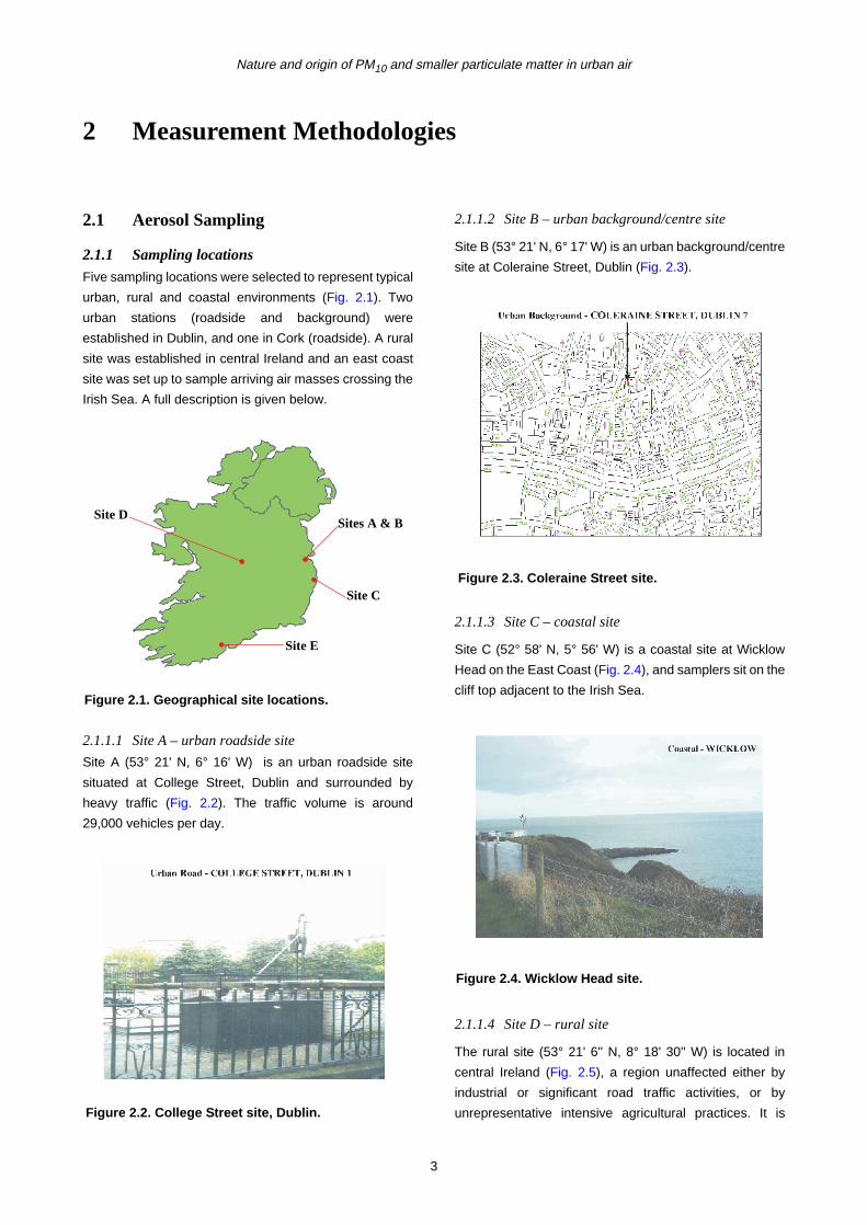
2.1.1 Sampling locationsFive sampling locations were selected to represent typical
urban, rural and coastal environments (Fig. 2.1). Two
urban stations (roadside and background) were
established in Dublin, and one in Cork (roadside). A rural
site was established in central Ireland and an east coast
site was set up to sample arriving air masses crossing the
Irish Sea. A full description is given below.
2.1.1.1 Site A – urban roadside site
Site A (53° 21' N, 6° 16' W) is an urban roadside site
situated at College Street, Dublin and surrounded by
heavy traffic (Fig. 2.2). The traffic volume is around
29,000 vehicles per day.
2.1.1.2 Site B – urban background/centre site
Site B (53° 21' N, 6° 17' W) is an urban background/centre
site at Coleraine Street, Dublin (Fig. 2.3).
2.1.1.3 Site C – coastal site
Site C (52° 58' N, 5° 56' W) is a coastal site at Wicklow
Head on the East Coast (Fig. 2.4), and samplers sit on the
cliff top adjacent to the Irish Sea.
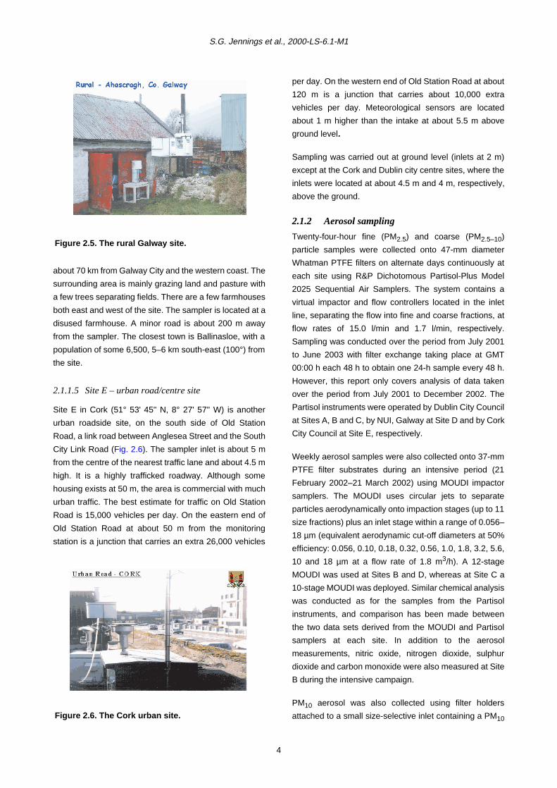
2.1.1.4 Site D – rural site
The rural site (53° 21' 6'' N, 8° 18' 30'' W) is located in
central Ireland (Fig. 2.5), a region unaffected either by
industrial or significant road traffic activities, or by
unrepresentative intensive agricultural practices. It is
Figure 2.1. Geographical site locations.
Sites A & B
Site C
Site E
Site D
Figure 2.2. College Street site, Dublin.
Figure 2.3. Coleraine Street site.
Figure 2.4. Wicklow Head site.
3
S.G. Jennings et al., 2000-LS-6.1-M1
about 70 km from Galway City and the western coast. The
surrounding area is mainly grazing land and pasture with
a few trees separating fields. There are a few farmhouses
both east and west of the site. The sampler is located at a
disused farmhouse. A minor road is about 200 m away
from the sampler. The closest town is Ballinasloe, with a
population of some 6,500, 5–6 km south-east (100°) from
the site.
2.1.1.5 Site E – urban road/centre site
Site E in Cork (51° 53' 45'' N, 8° 27' 57'' W) is another
urban roadside site, on the south side of Old Station
Road, a link road between Anglesea Street and the South
City Link Road (Fig. 2.6). The sampler inlet is about 5 m
from the centre of the nearest traffic lane and about 4.5 m
high. It is a highly trafficked roadway. Although some
housing exists at 50 m, the area is commercial with much
urban traffic. The best estimate for traffic on Old Station
Road is 15,000 vehicles per day. On the eastern end of
Old Station Road at about 50 m from the monitoring
station is a junction that carries an extra 26,000 vehicles
per day. On the western end of Old Station Road at about
120 m is a junction that carries about 10,000 extra
vehicles per day. Meteorological sensors are located
about 1 m higher than the intake at about 5.5 m above
ground level.
Sampling was carried out at ground level (inlets at 2 m)
except at the Cork and Dublin city centre sites, where the
inlets were located at about 4.5 m and 4 m, respectively,
above the ground.
2.1.2 Aerosol sampling
Twenty-four-hour fine (PM2.5) and coarse (PM2.5–10)
particle samples were collected onto 47-mm diameter
Whatman PTFE filters on alternate days continuously at
each site using R&P Dichotomous Partisol-Plus Model
2025 Sequential Air Samplers. The system contains a
virtual impactor and flow controllers located in the inlet
line, separating the flow into fine and coarse fractions, at
flow rates of 15.0 l/min and 1.7 l/min, respectively.
Sampling was conducted over the period from July 2001
to June 2003 with filter exchange taking place at GMT
00:00 h each 48 h to obtain one 24-h sample every 48 h.
However, this report only covers analysis of data taken
over the period from July 2001 to December 2002. The
Partisol instruments were operated by Dublin City Council
at Sites A, B and C, by NUI, Galway at Site D and by Cork
City Council at Site E, respectively.
Weekly aerosol samples were also collected onto 37-mm
PTFE filter substrates during an intensive period (21
February 2002–21 March 2002) using MOUDI impactor
samplers. The MOUDI uses circular jets to separate
particles aerodynamically onto impaction stages (up to 11
size fractions) plus an inlet stage within a range of 0.056–
18 µm (equivalent aerodynamic cut-off diameters at 50%
efficiency: 0.056, 0.10, 0.18, 0.32, 0.56, 1.0, 1.8, 3.2, 5.6,
10 and 18 µm at a flow rate of 1.8 m3/h). A 12-stage
MOUDI was used at Sites B and D, whereas at Site C a
10-stage MOUDI was deployed. Similar chemical analysis
was conducted as for the samples from the Partisol
instruments, and comparison has been made between
the two data sets derived from the MOUDI and Partisol
samplers at each site. In addition to the aerosol
measurements, nitric oxide, nitrogen dioxide, sulphur
dioxide and carbon monoxide were also measured at Site
B during the intensive campaign.
PM10 aerosol was also collected using filter holders
attached to a small size-selective inlet containing a PM10
Figure 2.5. The rural Galway site.
Figure 2.6. The Cork urban site.
4
Nature and origin of PM10 and smaller particulate matter in urban air
impactor at a flow rate of 8.5 l/min (Luhana, 1995). The
collection was conducted for two periods before the main
sampling campaign and during the intensive period, and
the samples used to provide information on the ratios of
OC to EC and on the calibration of EC content of the
exposed Partisol and MOUDI filters, determined using an
EEL reflectometer. Details of measurement, analysis and
calibration are described in Section 2.2.3.
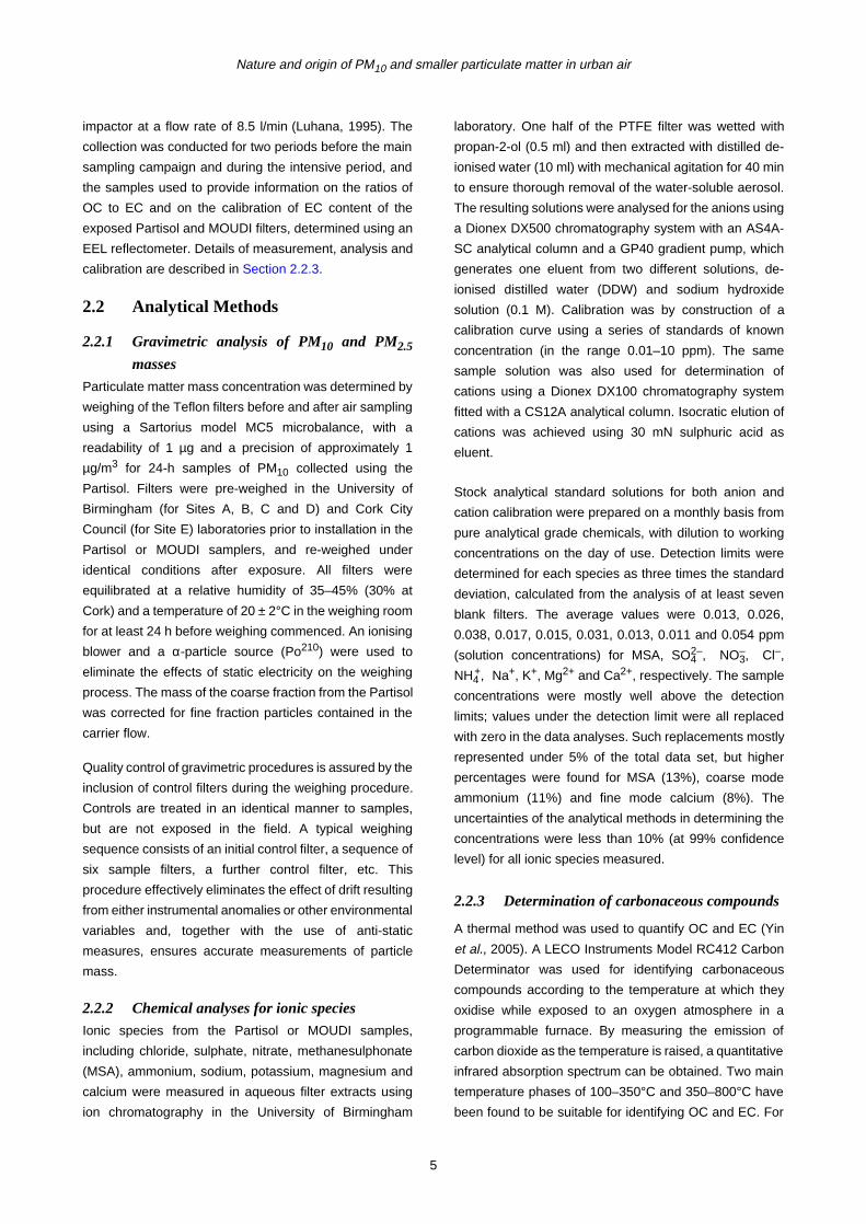
2.2 Analytical Methods
2.2.1 Gravimetric analysis of PM10 and PM2.5
masses
Particulate matter mass concentration was determined by
weighing of the Teflon filters before and after air sampling
using a Sartorius model MC5 microbalance, with a
readability of 1 µg and a precision of approximately 1
µg/m3 for 24-h samples of PM10 collected using the
Partisol. Filters were pre-weighed in the University of
Birmingham (for Sites A, B, C and D) and Cork City
Council (for Site E) laboratories prior to installation in the
Partisol or MOUDI samplers, and re-weighed under
identical conditions after exposure. All filters were
equilibrated at a relative humidity of 35–45% (30% at
Cork) and a temperature of 20 ± 2°C in the weighing room
for at least 24 h before weighing commenced. An ionising
blower and a α-particle source (Po210) were used to
eliminate the effects of static electricity on the weighing
process. The mass of the coarse fraction from the Partisol
was corrected for fine fraction particles contained in the
carrier flow.
Quality control of gravimetric procedures is assured by the
inclusion of control filters during the weighing procedure.
Controls are treated in an identical manner to samples,
but are not exposed in the field. A typical weighing
sequence consists of an initial control filter, a sequence of
six sample filters, a further control filter, etc. This
procedure effectively eliminates the effect of drift resulting
from either instrumental anomalies or other environmental
variables and, together with the use of anti-static
measures, ensures accurate measurements of particle
mass.
2.2.2 Chemical analyses for ionic species
Ionic species from the Partisol or MOUDI samples,
including chloride, sulphate, nitrate, methanesulphonate
(MSA), ammonium, sodium, potassium, magnesium and
calcium were measured in aqueous filter extracts using
ion chromatography in the University of Birmingham
laboratory. One half of the PTFE filter was wetted with
propan-2-ol (0.5 ml) and then extracted with distilled de-
ionised water (10 ml) with mechanical agitation for 40 min
to ensure thorough removal of the water-soluble aerosol.
The resulting solutions were analysed for the anions using
a Dionex DX500 chromatography system with an AS4A-
SC analytical column and a GP40 gradient pump, which
generates one eluent from two different solutions, de-
ionised distilled water (DDW) and sodium hydroxide
solution (0.1 M). Calibration was by construction of a
calibration curve using a series of standards of known
concentration (in the range 0.01–10 ppm). The same
sample solution was also used for determination of
cations using a Dionex DX100 chromatography system
fitted with a CS12A analytical column. Isocratic elution of
cations was achieved using 30 mN sulphuric acid as
eluent.
Stock analytical standard solutions for both anion and
cation calibration were prepared on a monthly basis from
pure analytical grade chemicals, with dilution to working
concentrations on the day of use. Detection limits were
determined for each species as three times the standard
deviation, calculated from the analysis of at least seven
blank filters. The average values were 0.013, 0.026,
0.038, 0.017, 0.015, 0.031, 0.013, 0.011 and 0.054 ppm
(solution concentrations) for MSA, SO42–, NO3
–, Cl–,
NH4+, Na+, K+, Mg2+ and Ca2+, respectively. The sample
concentrations were mostly well above the detection
limits; values under the detection limit were all replaced
with zero in the data analyses. Such replacements mostly
represented under 5% of the total data set, but higher
percentages were found for MSA (13%), coarse mode
ammonium (11%) and fine mode calcium (8%). The
uncertainties of the analytical methods in determining the
concentrations were less than 10% (at 99% confidence
level) for all ionic species measured.
2.2.3 Determination of carbonaceous compounds
A thermal method was used to quantify OC and EC (Yin
et al., 2005). A LECO Instruments Model RC412 Carbon
Determinator was used for identifying carbonaceous
compounds according to the temperature at which they
oxidise while exposed to an oxygen atmosphere in a
programmable furnace. By measuring the emission of
carbon dioxide as the temperature is raised, a quantitative
infrared absorption spectrum can be obtained. Two main
temperature phases of 100–350°C and 350–800°C have
been found to be suitable for identifying OC and EC. For
5

S.G. Jennings et al., 2000-LS-6.1-M1
eliminating moisture, a short phase at 100°C was used
initially. The instrument was calibrated using calcium
carbonate (which contains 12% carbon) as a standard
and also checked against organic compounds of known
composition. The detection limits for OC and EC were 6.1
and 4.5 µg, respectively, with method uncertainty about
±8.2% (at 99% confidence level). QMA (quartz) filters
were used for the above analysis during an initial phase of
the project and intensive periods. Pre-heating of filters at
500°C in air using a furnace prior to air sampling was
performed for eliminating any volatilisable impurities and
reducing the carbon blank values. It is noted that this
method may cause some overestimation of EC due to
charring of OC during pyrolysis (Schmid et al., 2001);
however, no established standard procedure has been
published.
The EC content of the exposed PTFE Partisol and MOUDI
filters was determined using an EEL reflectometer by
measuring their blackness (i.e. light absorbance). These
absorption data were calibrated against the thermal
method (above), based on the assumption that EC is the
principal light-absorbing species in ambient air (Horvath,
1993, 1997).
Organic carbon from the PTFE samples was estimated
using EC data and the ratios of OC/EC. The ratios will
vary spatially and temporally, but a clear minimum ratio,
which increases from 1.1 in larger cities to 1.5 at rural and
remote sites, has been found in urban and rural European
atmospheres (Castro et al., 1999). OC/EC ratios were
determined according to season, either winter (October to
March) or summer (April to September), and
independently for fine and coarse fractions. Ratios were
based on direct measurements of PM10 elemental and
OC content at Sites B and C during an intensive
measurement period in February and March 2002, and of
PM10 and PM2.5 elemental and OC content at all sites
during January 2003. OC/EC ratios used for calculation of
the OC contents during summer (April to September)
were adjusted (separately for urban and non-urban sites)
using previously reported seasonal values for European
sites (Castro et al., 1999; Yin, 2002). In urban areas, the
ratios used were 1.0 and 1.5 for fine and coarse particles
in winter, with corresponding values of 1.5 and 2.5 in
summer. At the non-urban sites (C and D), values
employed were 2.0 in winter and 3.0 in summer for both
fine and coarse particles. We estimate an OC/EC ratio
uncertainty of around 30%.
2.2.4 Chemical analysis for PAHs
Polyaromatic hydrocarbons (PAHs) were extracted from
the PTFE filters using the Soxhlet extraction method. The
filters were placed in the glass vessel and extracted with
dichloromethane (150 ml) for 18 h. The resulting mixture
was placed in a rotary evaporator to remove the
dichloromethane. The residue, containing the PAHs, was
dissolved in n-hexane (10 ml) and then reduced to a
volume of 1 ml through evaporation of the solvent. The
efficiency of the Soxhlet extraction procedure was tested
by using an appropriate Standard Reference Material
(Urban Particulate Matter 1649, NIST). Recoveries in the
range 90–107% were obtained thus confirming the high
efficiency of the method.
Determination of PAH concentrations was carried out by
GC–MS using a Varian GC3800 coupled to a Saturn 2000
ion trap mass spectrometer. The instrument was
equipped with an auto-sampler (CP-8400 series) and
controlled with Varian Saturn software. The GC–MS was
operated in electron ionisation (EI) mode over the mass
range 75–320 m/z. Chromatographic separation was
achieved was a CP-Sil8CB fused silica capillary column
(Chrompak, 30 m, 0.25 mm i.d., 0.25 µm film thickness)
which was operated at 35°C for 1 min and then increased
to 320°C at a rate of 10°C per minute and held for 5 min.
Samples were placed in the auto-sampler and volumes of
1 µl were injected using the splitless mode with an injector
temperature of 250°C. GC–MS calibration was carried out
using standard solutions containing 0.01–0.6 ng of the 16
US EPA priority PAHs in 1 µl of acetonitrile. Each sample,
including the calibration solutions, was injected three
times and an average value for the concentration was
obtained.
2.2.5 Chemical analysis for metals
Trace metals were extracted from the PTFE filters using a
microwave-assisted acid digestion method. The filters
were placed in fluoroplastic vessels, which were mounted
in ceramic supporting vessels, and a standard acid
digestion mixture consisting of HNO3 (65%, 2 ml), HF
(40%, 100 µl) and H2O (2 ml) was added (Jalkanen and
Hasanen, 1996; Robache et al., 2000). One reagent blank
for each digestion was also performed to check for
contamination during the process. The vessels were
inserted into the microwave (Anton Paar MULTIWAVE)
and a four-step programme, lasting 51 min, was used for
the digestion process. The digested samples were
transferred to volumetric flasks, the reaction vessels
6

Nature and origin of PM10 and smaller particulate matter in urban air
washed out with distilled water and the flask volume made
up to 15 ml with distilled water. The reaction vessels were
cleaned before each digestion using HNO3 (65%, 5 ml)
heated in the microwave at 1000 W for 30 min. The
efficiency of the microwave digestion procedure was
tested by using an appropriate Standard Reference
Material (Urban Particulate Matter 1648, NIST).
Recoveries in the range 91–102% were obtained thus
confirming the high efficiency of the method.
Metal determination was carried out by Inductively
Coupled Plasma–Atomic Emission Spectrometry (ICP–
AES) using a Perkin Elmer Optima 2000 DV Optical
Emission Spectrometer fitted with a pneumatic nebuliser
and a Scott spray chamber. The instrument was equipped
with an auto-sampler (AS-90 series) and controlled with
PE Winlab software. ICP–AES calibration was carried out
using standard solutions with concentrations of 21
elements between 10 ppb and 1 ppm in 5% nitric acid.
The solutions were prepared from a multi-elemental
standard solution containing 21 elements at levels of 100
mg/l in 5% nitric acid (Glen Spectra Reference Material).
Each sample, including the calibration solutions, was
sampled three times and an average value for the
concentration was obtained. In this work, the elements
analysed were crustal and anthropogenic trace metals
(Ca, Fe, Ni, Zn, Mg, Pb, Mn, Cr, V, Cd, Cu) chosen for
their biogeochemical impact on the terrestrial ecosystems
and their potential effects on human health. The
quantitation limits (based on 10δ of the blank) were
calculated in µg/l for each element and were 14, 2, 1, 6, 1,
3, 120, 2, 5, 2 and 2 for Ca, Mn, Fe, Ni, Zn, Mg, Pb, Cr, V,
Cd and Cu, respectively.
7
S.G. Jennings et al., 2000-LS-6.1-M1
3 Overview of Concentration Levels of PM10 and PM2.5Masses and their Chemical Components in the IrishAtmosphere
3.1 Atmospheric Concentrations ofParticle Mass
3.1.1 Long-term and short-term variation of PM
mass concentrations
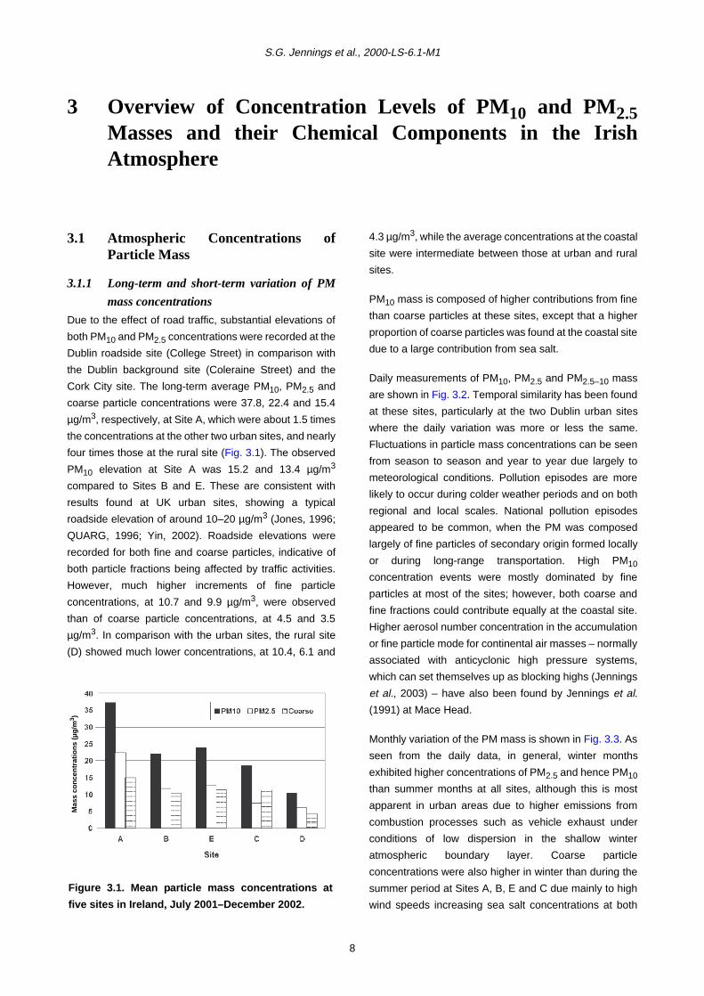
Due to the effect of road traffic, substantial elevations of
both PM10 and PM2.5 concentrations were recorded at the
Dublin roadside site (College Street) in comparison with
the Dublin background site (Coleraine Street) and the
Cork City site. The long-term average PM10, PM2.5 and
coarse particle concentrations were 37.8, 22.4 and 15.4
µg/m3, respectively, at Site A, which were about 1.5 times
the concentrations at the other two urban sites, and nearly
four times those at the rural site (Fig. 3.1). The observed
PM10 elevation at Site A was 15.2 and 13.4 µg/m3
compared to Sites B and E. These are consistent with
results found at UK urban sites, showing a typical
roadside elevation of around 10–20 µg/m3 (Jones, 1996;
QUARG, 1996; Yin, 2002). Roadside elevations were
recorded for both fine and coarse particles, indicative of
both particle fractions being affected by traffic activities.
However, much higher increments of fine particle
concentrations, at 10.7 and 9.9 µg/m3, were observed
than of coarse particle concentrations, at 4.5 and 3.5
µg/m3. In comparison with the urban sites, the rural site
(D) showed much lower concentrations, at 10.4, 6.1 and
4.3 µg/m3, while the average concentrations at the coastal
site were intermediate between those at urban and rural
sites.
PM10 mass is composed of higher contributions from fine
than coarse particles at these sites, except that a higher
proportion of coarse particles was found at the coastal site
due to a large contribution from sea salt.
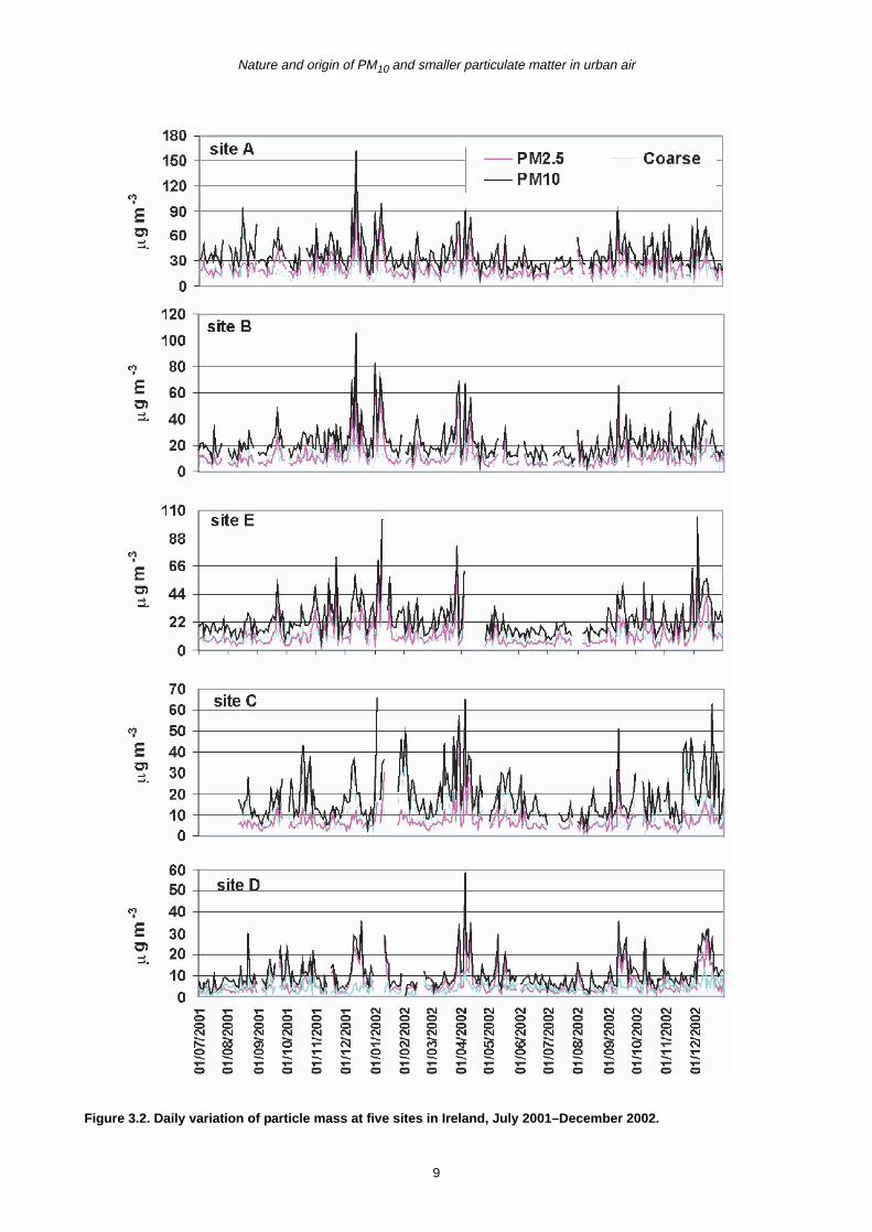
Daily measurements of PM10, PM2.5 and PM2.5–10 mass
are shown in Fig. 3.2. Temporal similarity has been found
at these sites, particularly at the two Dublin urban sites
where the daily variation was more or less the same.
Fluctuations in particle mass concentrations can be seen
from season to season and year to year due largely to
meteorological conditions. Pollution episodes are more
likely to occur during colder weather periods and on both
regional and local scales. National pollution episodes
appeared to be common, when the PM was composed
largely of fine particles of secondary origin formed locally
or during long-range transportation. High PM10
concentration events were mostly dominated by fine
particles at most of the sites; however, both coarse and
fine fractions could contribute equally at the coastal site.
Higher aerosol number concentration in the accumulation
or fine particle mode for continental air masses – normally
associated with anticyclonic high pressure systems,
which can set themselves up as blocking highs (Jennings
et al., 2003) – have also been found by Jennings et al.
(1991) at Mace Head.
Monthly variation of the PM mass is shown in Fig. 3.3. As
seen from the daily data, in general, winter months
exhibited higher concentrations of PM2.5 and hence PM10
than summer months at all sites, although this is most
apparent in urban areas due to higher emissions from
combustion processes such as vehicle exhaust under
conditions of low dispersion in the shallow winter
atmospheric boundary layer. Coarse particle
concentrations were also higher in winter than during the
summer period at Sites A, B, E and C due mainly to high
wind speeds increasing sea salt concentrations at both
Figure 3.1. Mean particle mass concentrations at
five sites in Ireland, July 2001–December 2002.
Mas
s co
nce
ntr
atio
ns
(µg
/m3 )
8
Nature and origin of PM10 and smaller particulate matter in urban air
Figure 3.2. Daily variation of particle mass at five sites in Ireland, July 2001–December 2002.
9

S.G. Jennings et al., 2000-LS-6.1-M1
Figure 3.3. Monthly variation of particle mass at five sites in Ireland, July 2001–December 2002.
10
Nature and origin of PM10 and smaller particulate matter in urban air
the coastal and the nearby Dublin and Cork sites. In
comparison, the central rural site showed the least effect
of this component. In addition, summer 2001 showed
higher coarse particle and hence PM10 levels at Site A,
presumably due to traffic or construction activity induced
resuspension of dust materials under dry and hot weather
conditions.
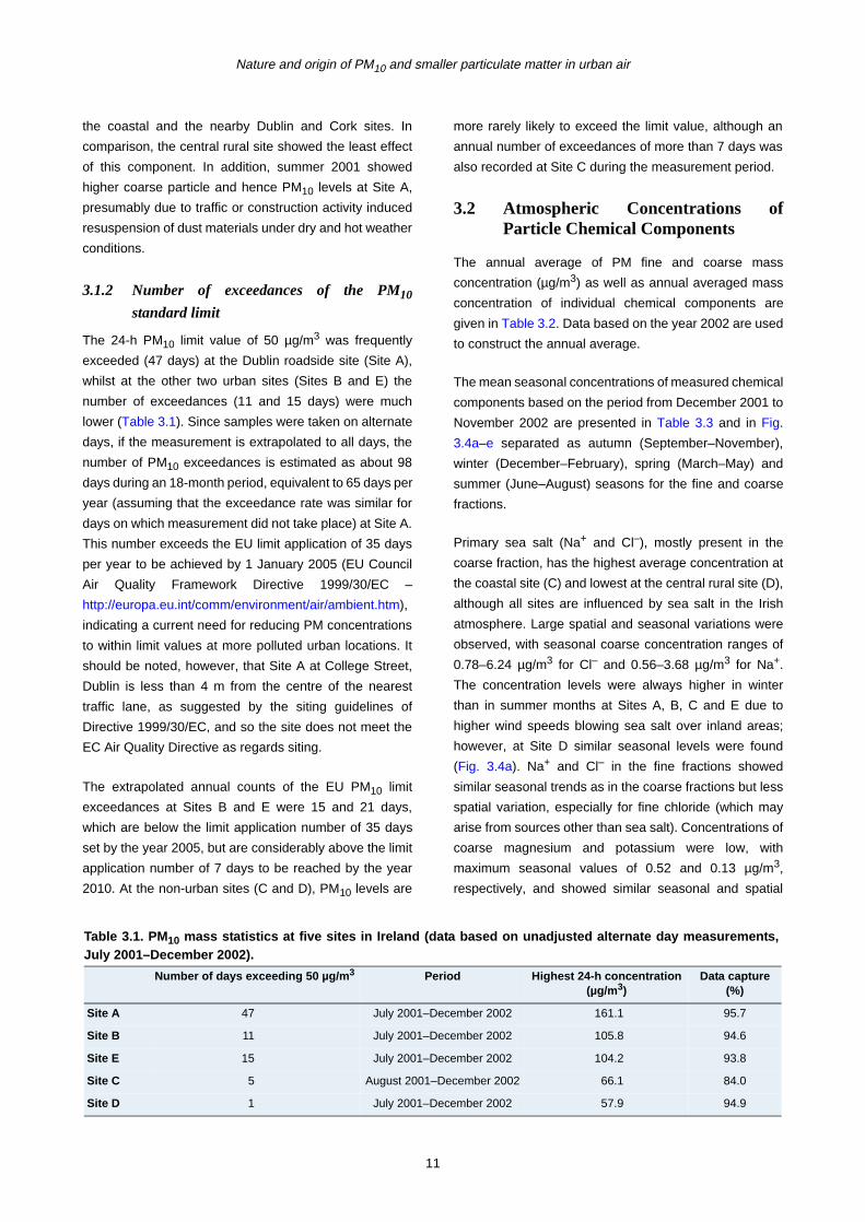
3.1.2 Number of exceedances of the PM10
standard limit
The 24-h PM10 limit value of 50 µg/m3 was frequently
exceeded (47 days) at the Dublin roadside site (Site A),
whilst at the other two urban sites (Sites B and E) the
number of exceedances (11 and 15 days) were much
lower (Table 3.1). Since samples were taken on alternate
days, if the measurement is extrapolated to all days, the
number of PM10 exceedances is estimated as about 98
days during an 18-month period, equivalent to 65 days per
year (assuming that the exceedance rate was similar for
days on which measurement did not take place) at Site A.
This number exceeds the EU limit application of 35 days
per year to be achieved by 1 January 2005 (EU Council
Air Quality Framework Directive 1999/30/EC –
http://europa.eu.int/comm/environment/air/ambient.htm),
indicating a current need for reducing PM concentrations
to within limit values at more polluted urban locations. It
should be noted, however, that Site A at College Street,
Dublin is less than 4 m from the centre of the nearest
traffic lane, as suggested by the siting guidelines of
Directive 1999/30/EC, and so the site does not meet the
EC Air Quality Directive as regards siting.
The extrapolated annual counts of the EU PM10 limit
exceedances at Sites B and E were 15 and 21 days,
which are below the limit application number of 35 days
set by the year 2005, but are considerably above the limit
application number of 7 days to be reached by the year
2010. At the non-urban sites (C and D), PM10 levels are
more rarely likely to exceed the limit value, although an
annual number of exceedances of more than 7 days was
also recorded at Site C during the measurement period.
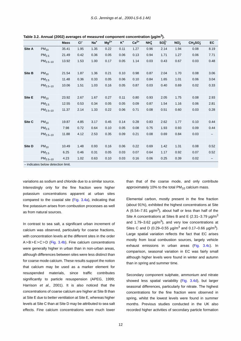
3.2 Atmospheric Concentrations ofParticle Chemical Components
The annual average of PM fine and coarse mass
concentration (µg/m3) as well as annual averaged mass
concentration of individual chemical components are
given in Table 3.2. Data based on the year 2002 are used
to construct the annual average.
The mean seasonal concentrations of measured chemical
components based on the period from December 2001 to
November 2002 are presented in Table 3.3 and in Fig.
3.4a–e separated as autumn (September–November),
winter (December–February), spring (March–May) and
summer (June–August) seasons for the fine and coarse
fractions.
Primary sea salt (Na+ and Cl–), mostly present in the
coarse fraction, has the highest average concentration at
the coastal site (C) and lowest at the central rural site (D),
although all sites are influenced by sea salt in the Irish
atmosphere. Large spatial and seasonal variations were
observed, with seasonal coarse concentration ranges of
0.78–6.24 µg/m3 for Cl– and 0.56–3.68 µg/m3 for Na+.
The concentration levels were always higher in winter
than in summer months at Sites A, B, C and E due to
higher wind speeds blowing sea salt over inland areas;
however, at Site D similar seasonal levels were found
(Fig. 3.4a). Na+ and Cl– in the fine fractions showed
similar seasonal trends as in the coarse fractions but less
spatial variation, especially for fine chloride (which may
arise from sources other than sea salt). Concentrations of
coarse magnesium and potassium were low, with
maximum seasonal values of 0.52 and 0.13 µg/m3,
respectively, and showed similar seasonal and spatial
Table 3.1. PM10 mass statistics at five sites in Ireland (data based on unadjusted alternate day measurements,July 2001–December 2002).
Number of days exceeding 50 µg/m3 Period Highest 24-h concentration(µg/m3)
Data capture(%)
Site A 47 July 2001–December 2002 161.1 95.7
Site B 11 July 2001–December 2002 105.8 94.6
Site E 15 July 2001–December 2002 104.2 93.8
Site C 5 August 2001–December 2002 66.1 84.0
Site D 1 July 2001–December 2002 57.9 94.9
11
S.G. Jennings et al., 2000-LS-6.1-M1
variations as sodium and chloride due to a similar source.
Interestingly only for the fine fraction were higher
potassium concentrations apparent at urban sites
compared to the coastal site (Fig. 3.4a), indicating that
fine potassium arises from combustion processes as well
as from natural sources.
In contrast to sea salt, a significant urban increment of
calcium was observed, particularly for coarse fractions,
with concentration levels at the different sites in the order
A > B > E > C > D (Fig. 3.4b). Fine calcium concentrations
were generally higher in urban than in non-urban areas,
although differences between sites were less distinct than
for coarse mode calcium. These results support the notion
that calcium may be used as a marker element for
resuspended materials, since traffic contributes
significantly to particle resuspension (APEG, 1999;
Harrison et al., 2001). It is also noticed that the
concentrations of coarse calcium are higher at Site B than
at Site E due to better ventilation at Site E, whereas higher
levels at Site C than at Site D may be attributed to sea salt
effects. Fine calcium concentrations were much lower
than that of the coarse mode, and only contribute
approximately 10% to the total PM10 calcium mass.
Elemental carbon, mostly present in the fine fraction
(about 91%), exhibited the highest concentrations at Site
A (6.54–7.81 µg/m3), about half or less than half of the
Site A concentrations at Sites B and E (2.31–3.79 µg/m3
and 1.79–3.62 µg/m3), and very low concentrations at
Sites C and D (0.29–0.55 µg/m3 and 0.17–0.66 µg/m3).
Large spatial variation reflects the fact that EC arises
mostly from local combustion sources, largely vehicle
exhaust emissions in urban areas (Fig. 3.4c). In
comparison, seasonal variation in EC was fairly small
although higher levels were found in winter and autumn
than in spring and summer time.
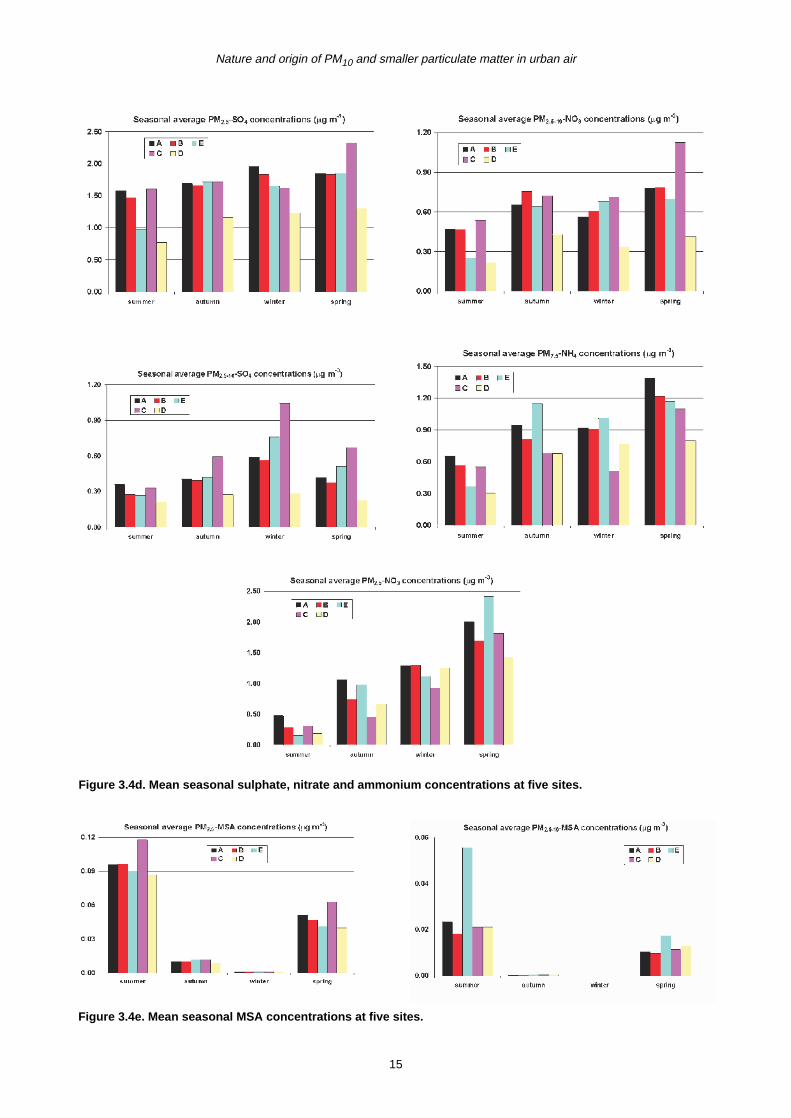
Secondary component sulphate, ammonium and nitrate
showed less spatial variability (Fig. 3.4d), but larger
seasonal differences, particularly for nitrate. The highest
concentrations for the fine fraction were observed in
spring, whilst the lowest levels were found in summer
months. Previous studies conducted in the UK also
recorded higher activities of secondary particle formation
Table 3.2. Annual (2002) averages of measured component concentration ( µg/m 3).
Mass Cl– Na+ Mg2+ K+ Ca2+ NH4+ SO4
2– NO3– CH3SO2
– EC
Site A PM10 35.41 1.95 1.35 0.22 0.11 1.27 0.96 2.14 1.94 0.08 8.19
PM2.5 21.49 0.42 0.36 0.05 0.06 0.13 0.94 1.71 1.27 0.06 7.71
PM2.5–10 13.92 1.53 1.00 0.17 0.05 1.14 0.03 0.43 0.67 0.03 0.48
Site B PM10 21.54 1.87 1.36 0.21 0.10 0.98 0.87 2.04 1.70 0.08 3.06
PM2.5 11.48 0.36 0.33 0.05 0.06 0.10 0.84 1.65 1.01 0.06 3.04
PM2.5–10 10.06 1.51 1.03 0.16 0.05 0.87 0.03 0.40 0.69 0.02 0.33
Site E PM10 23.92 2.67 1.67 0.27 0.11 0.80 0.93 2.05 1.75 0.08 2.93
PM2.5 12.55 0.53 0.34 0.05 0.05 0.09 0.87 1.54 1.16 0.06 2.81
PM2.5–10 11.37 2.14 1.33 0.22 0.06 0.71 0.08 0.51 0.60 0.03 0.28
Site C PM10 19.87 4.85 3.17 0.45 0.14 0.28 0.83 2.62 1.77 0.10 0.44
PM2.5 7.98 0.72 0.64 0.10 0.05 0.08 0.75 1.93 0.93 0.09 0.44
PM2.5–10 11.88 4.12 2.53 0.35 0.09 0.21 0.08 0.69 0.84 0.03 –
Site D PM10 10.49 1.48 0.93 0.16 0.06 0.22 0.69 1.42 1.31 0.08 0.52
PM2.5 6.25 0.46 0.31 0.05 0.03 0.07 0.64 1.17 0.92 0.07 0.52
PM2.5–10 4.23 1.02 0.63 0.10 0.03 0.16 0.06 0.25 0.39 0.02 –
– indicates below detection limit.
12

Nature and origin of PM10 and smaller particulate matter in urban air
Table 3.3. Seasonal mean concentrations (µg/m 3) of measured chemical components at five sites in Ireland,December 2001–November 2002.
Cl– Na+ Mg2+ K+ Ca2+ NH4+ SO4
2– NO3– CH3SO3
– EC
Site A Fine Autumn 0.46 0.35 0.05 0.10 0.16 0.95 1.70 1.06 0.01 7.65
Winter 0.88 0.50 0.08 0.08 0.18 0.92 1.96 1.28 – 7.81
Spring 0.32 0.45 0.06 0.05 0.12 1.39 1.85 2.00 0.05 6.54
Summer 0.16 0.23 0.04 0.06 0.18 0.65 1.58 0.47 0.10 7.10
Coarse Autumn 1.34 0.87 0.15 0.06 1.32 0.03 0.41 0.66 – 0.71
Winter 2.16 1.32 0.22 0.05 1.31 0.01 0.59 0.56 – 0.62
Spring 1.65 1.27 0.19 0.03 1.22 0.03 0.42 0.78 0.01 0.48
Summer 0.82 0.60 0.12 0.07 1.58 0.01 0.36 0.47 0.02 0.53
Site B Fine Autumn 0.30 0.30 0.04 0.08 0.15 0.81 1.66 0.74 0.01 3.37
Winter 0.77 0.45 0.07 0.08 0.15 0.91 1.83 1.30 – 3.79
Spring 0.28 0.46 0.06 0.05 0.11 1.21 1.83 1.69 0.05 2.56
Summer 0.14 0.22 0.03 0.04 0.09 0.57 1.47 0.28 0.10 2.31
Coarse Autumn 1.45 0.99 0.15 0.06 1.09 0.04 0.39 0.76 – –
Winter 2.14 1.34 0.22 0.05 0.93 0.02 0.56 0.61 – 0.19
Spring 1.55 1.32 0.18 0.03 1.01 0.02 0.37 0.79 0.01 –
Summer 0.78 0.58 0.11 0.05 0.84 0.02 0.28 0.47 0.02 –
Site E Fine Autumn 0.51 0.33 0.05 0.07 0.15 1.15 1.72 0.98 0.01 3.43
Winter 0.93 0.45 0.07 0.07 0.11 1.01 1.65 1.12 – 3.62
Spring 0.53 0.40 0.06 0.04 0.09 1.17 1.85 2.42 0.04 2.46
Summer 0.21 0.24 0.04 0.05 0.13 0.37 0.97 0.16 0.09 1.79
Coarse Autumn 2.00 1.34 0.20 0.08 0.76 0.06 0.42 0.64 – –
Winter 2.96 1.85 0.30 0.08 0.77 0.11 0.76 0.68 – 0.28
Spring 2.20 1.39 0.22 0.05 0.68 0.05 0.51 0.70 0.02 –
Summer 1.18 0.86 0.13 0.06 0.65 0.01 0.27 0.25 0.06 –
Site C Fine Autumn 0.65 0.59 0.08 0.05 0.09 0.68 1.72 0.45 0.01 0.48
Winter 1.17 0.93 0.14 0.05 0.11 0.51 1.62 0.93 – 0.51
Spring 0.67 0.69 0.11 0.04 0.05 1.10 2.33 1.82 0.06 0.55
Summer 0.24 0.36 0.06 0.04 0.06 0.55 1.61 0.30 0.12 0.29
Coarse Autumn 3.58 2.38 0.30 0.10 0.22 0.08 0.59 0.72 – –
Winter 6.24 3.68 0.52 0.13 0.27 0.06 1.04 0.72 – –
Spring 4.07 2.66 0.35 0.07 0.21 0.11 0.67 1.13 0.01 –
Summer 1.69 1.28 0.19 0.07 0.13 0.03 0.33 0.54 0.02 –
Site D Fine Autumn 0.32 0.26 0.04 0.04 0.06 0.68 1.16 0.67 0.01 0.42
Winter 0.80 0.43 0.07 0.04 0.12 0.77 1.23 1.25 – 0.66
Spring 0.46 0.35 0.06 0.02 0.05 0.80 1.30 1.42 0.04 0.44
Summer 0.19 0.20 0.03 0.02 0.04 0.31 0.77 0.18 0.09 –
Coarse Autumn 1.12 0.74 0.10 0.04 0.19 0.07 0.28 0.43 – –
Winter 0.96 0.60 0.10 0.03 0.18 0.04 0.29 0.34 – –
Spring 1.14 0.73 0.12 0.02 0.16 0.03 0.23 0.41 0.01 –
Summer 0.80 0.56 0.09 0.05 0.16 0.02 0.21 0.22 0.02 –
– indicates below detection limit.
13

S.G. Jennings et al., 2000-LS-6.1-M1
in spring (Yin, 2002). About three-quarters to four-fifths of
SO42– and two-thirds of NO3
– were present in the fine
fractions at these sites, and very little NH4+ was found in
the coarse fractions.
Despite very low concentrations (0.0–0.12 µg/m3), the
maximum production of MSA occurred in summer, with
little production in spring and autumn while wintertime
often showed zero values. There was no clear spatial
trend although higher levels were observed at Site C for
fine MSA and at Site E for the coarse fraction (Fig. 3.4e).
MSA can be present in both fine and coarse fractions but
a higher proportion was normally found in the fine mode.
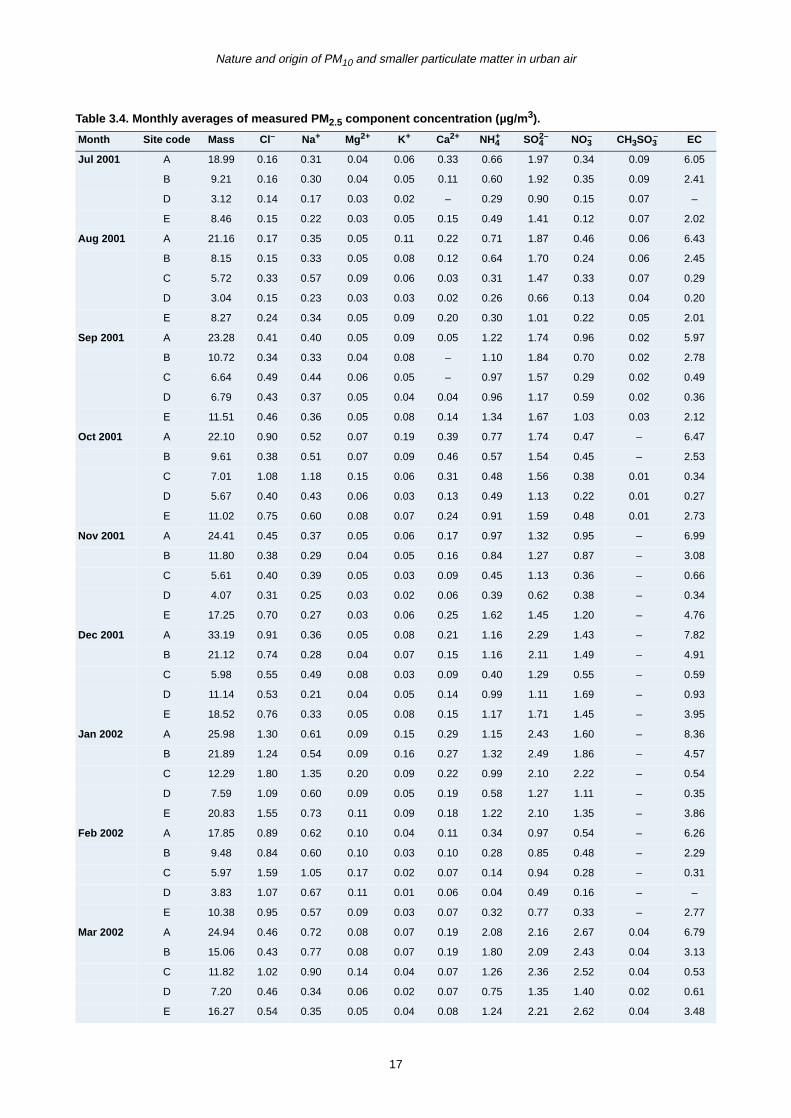
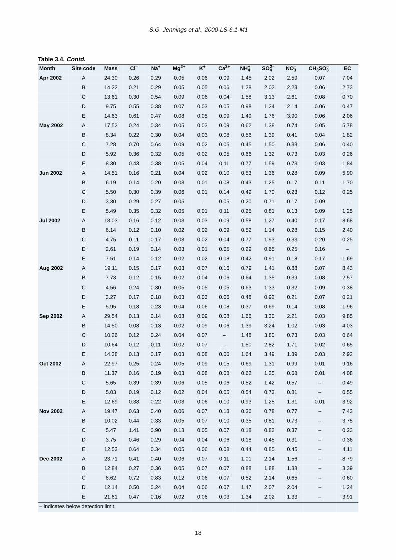
3.3 Relationship between Monthly PMMass and its Major ChemicalComponent Concentrations
The monthly average mass concentrations (µg/m3) of
measured chemical components at the five sites over the
Figure 3.4a. Mean seasonal sea salt concentrations
at five sites.
Figure 3.4b. Mean seasonal calcium concentrations
at five sites.
Figure 3.4c. Mean seasonal elemental carbon
concentrations at five sites.
14
Nature and origin of PM10 and smaller particulate matter in urban air
Figure 3.4d. Mean seasonal sulphate, nitrate and ammonium concentrations at five sites.
Figure 3.4e. Mean seasonal MSA concentrations at five sites.
15

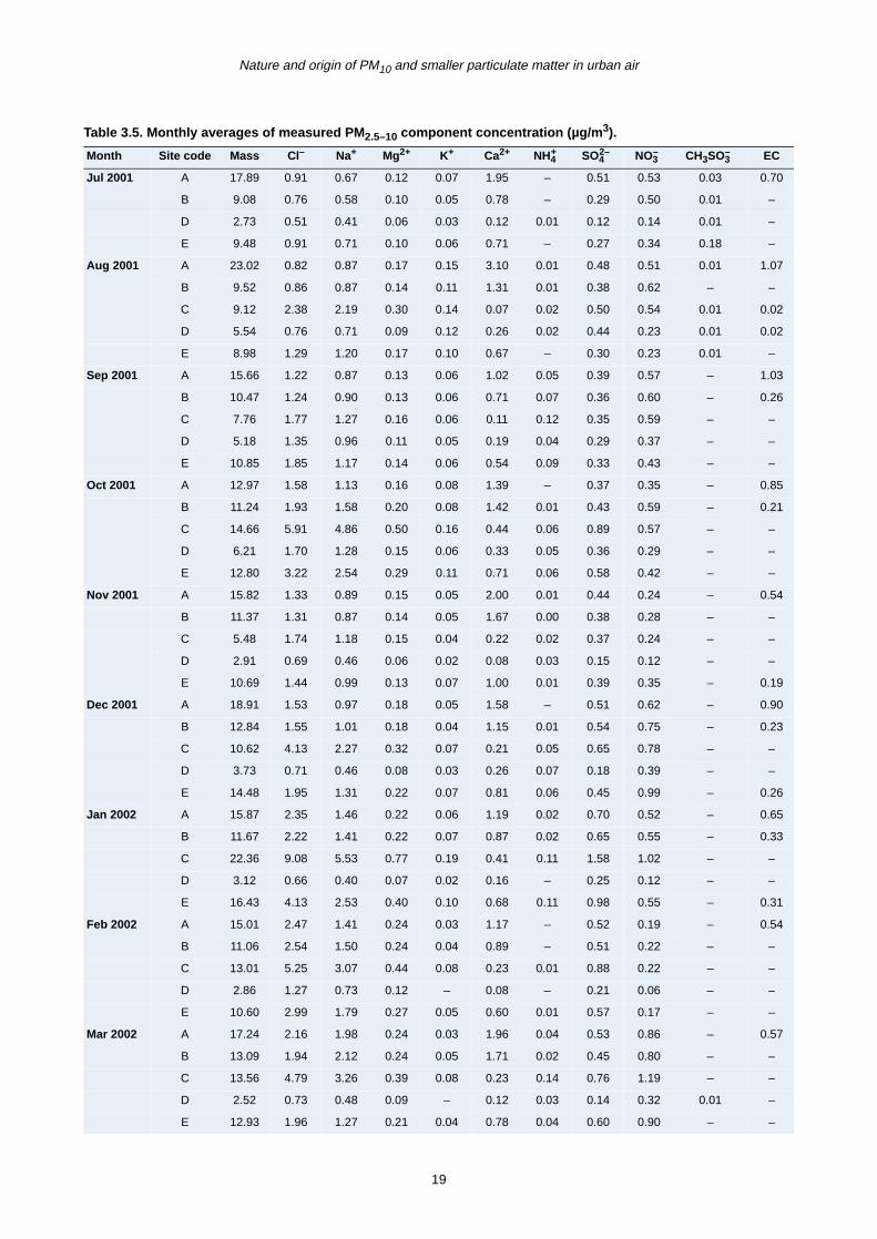
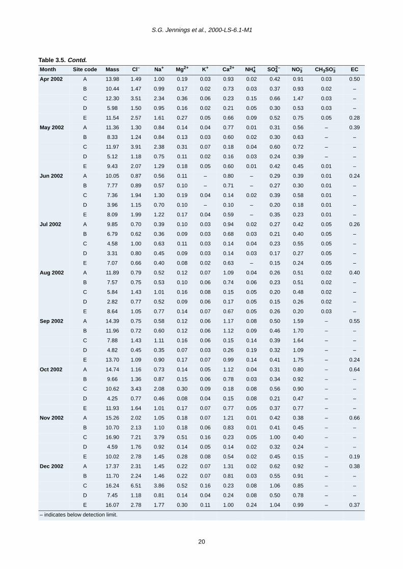
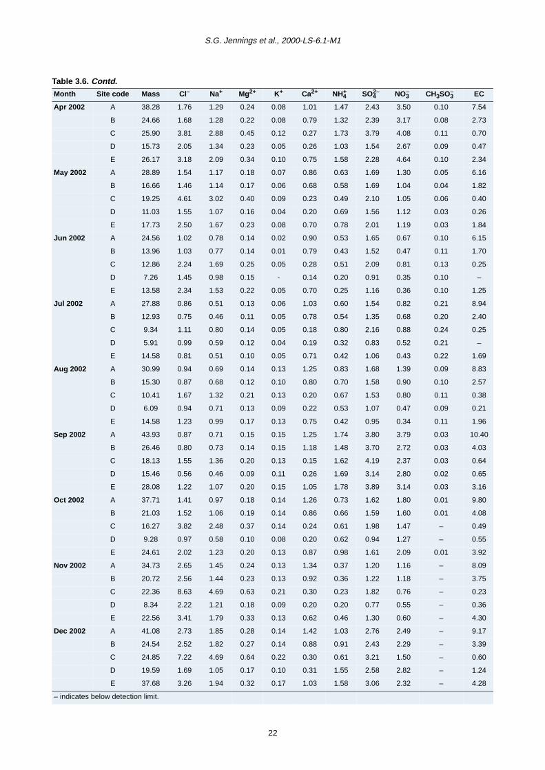
S.G. Jennings et al., 2000-LS-6.1-M1
period from June 2001 to December 2002 are presented
in Tables 3.4–3.6 for fine (PM2.5) and coarse (PM2.5–10
and PM10) mode particles. Total mass concentration
(µg/m3) for the three modes is also given.
Monthly time series are illustrated in Figs 3.5a and 3.5b
for both fine and coarse particle fractions at each site. The
correlation between the total mass and its chemical
component mass, and the relative importance of a
chemical component in contributing to the aerosol mass,
were examined at each site.
The major chemical species contributing to fine particles
are EC, sulphate, nitrate and ammonium (Fig. 3.5a). In
general, good correlation was observed between PM2.5
and these chemical components at all sites except at Site
E where temporal inconsistency was observed. In urban
areas, a greater contribution to the fine mass was found
from primary EC than from inorganic secondary materials.
This is particularly apparent at the Dublin roadside site. At
non-urban locations, it is found that secondary source
particles make a greater contribution than EC to the fine
mass .
The correlation between coarse particle mass and its
major chemical components (calcium, chloride, sodium
and nitrate) was less clear (Fig. 3.5b). At Sites A and B, a
better relationship was found between PM2.5–10 and
calcium, although both sea salt and calcium were the
most significant chemical components. Conversely at
Sites E and D, sea salt exhibited the highest correlation
with coarse mass and calcium was less important. It must
be pointed out that very good correlation between sea salt
and the coarse mass was only found at the coastal site
(C), where sea salt is also the major chemical component
of the aerosol mass.
16
Nature and origin of PM10 and smaller particulate matter in urban air
Table 3.4. Monthly averages of measured PM2.5 component concentration (µg/m 3).
Month Site code Mass Cl– Na+ Mg2+ K+ Ca2+ NH4+ SO4
2– NO3– CH3SO3
– EC
Jul 2001 A 18.99 0.16 0.31 0.04 0.06 0.33 0.66 1.97 0.34 0.09 6.05
B 9.21 0.16 0.30 0.04 0.05 0.11 0.60 1.92 0.35 0.09 2.41
D 3.12 0.14 0.17 0.03 0.02 – 0.29 0.90 0.15 0.07 –
E 8.46 0.15 0.22 0.03 0.05 0.15 0.49 1.41 0.12 0.07 2.02
Aug 2001 A 21.16 0.17 0.35 0.05 0.11 0.22 0.71 1.87 0.46 0.06 6.43
B 8.15 0.15 0.33 0.05 0.08 0.12 0.64 1.70 0.24 0.06 2.45
C 5.72 0.33 0.57 0.09 0.06 0.03 0.31 1.47 0.33 0.07 0.29
D 3.04 0.15 0.23 0.03 0.03 0.02 0.26 0.66 0.13 0.04 0.20
E 8.27 0.24 0.34 0.05 0.09 0.20 0.30 1.01 0.22 0.05 2.01
Sep 2001 A 23.28 0.41 0.40 0.05 0.09 0.05 1.22 1.74 0.96 0.02 5.97
B 10.72 0.34 0.33 0.04 0.08 – 1.10 1.84 0.70 0.02 2.78
C 6.64 0.49 0.44 0.06 0.05 – 0.97 1.57 0.29 0.02 0.49
D 6.79 0.43 0.37 0.05 0.04 0.04 0.96 1.17 0.59 0.02 0.36
E 11.51 0.46 0.36 0.05 0.08 0.14 1.34 1.67 1.03 0.03 2.12
Oct 2001 A 22.10 0.90 0.52 0.07 0.19 0.39 0.77 1.74 0.47 – 6.47
B 9.61 0.38 0.51 0.07 0.09 0.46 0.57 1.54 0.45 – 2.53
C 7.01 1.08 1.18 0.15 0.06 0.31 0.48 1.56 0.38 0.01 0.34
D 5.67 0.40 0.43 0.06 0.03 0.13 0.49 1.13 0.22 0.01 0.27
E 11.02 0.75 0.60 0.08 0.07 0.24 0.91 1.59 0.48 0.01 2.73
Nov 2001 A 24.41 0.45 0.37 0.05 0.06 0.17 0.97 1.32 0.95 – 6.99
B 11.80 0.38 0.29 0.04 0.05 0.16 0.84 1.27 0.87 – 3.08
C 5.61 0.40 0.39 0.05 0.03 0.09 0.45 1.13 0.36 – 0.66
D 4.07 0.31 0.25 0.03 0.02 0.06 0.39 0.62 0.38 – 0.34
E 17.25 0.70 0.27 0.03 0.06 0.25 1.62 1.45 1.20 – 4.76
Dec 2001 A 33.19 0.91 0.36 0.05 0.08 0.21 1.16 2.29 1.43 – 7.82
B 21.12 0.74 0.28 0.04 0.07 0.15 1.16 2.11 1.49 – 4.91
C 5.98 0.55 0.49 0.08 0.03 0.09 0.40 1.29 0.55 – 0.59
D 11.14 0.53 0.21 0.04 0.05 0.14 0.99 1.11 1.69 – 0.93
E 18.52 0.76 0.33 0.05 0.08 0.15 1.17 1.71 1.45 – 3.95
Jan 2002 A 25.98 1.30 0.61 0.09 0.15 0.29 1.15 2.43 1.60 – 8.36
B 21.89 1.24 0.54 0.09 0.16 0.27 1.32 2.49 1.86 – 4.57
C 12.29 1.80 1.35 0.20 0.09 0.22 0.99 2.10 2.22 – 0.54
D 7.59 1.09 0.60 0.09 0.05 0.19 0.58 1.27 1.11 – 0.35
E 20.83 1.55 0.73 0.11 0.09 0.18 1.22 2.10 1.35 – 3.86
Feb 2002 A 17.85 0.89 0.62 0.10 0.04 0.11 0.34 0.97 0.54 – 6.26
B 9.48 0.84 0.60 0.10 0.03 0.10 0.28 0.85 0.48 – 2.29
C 5.97 1.59 1.05 0.17 0.02 0.07 0.14 0.94 0.28 – 0.31
D 3.83 1.07 0.67 0.11 0.01 0.06 0.04 0.49 0.16 – –
E 10.38 0.95 0.57 0.09 0.03 0.07 0.32 0.77 0.33 – 2.77
Mar 2002 A 24.94 0.46 0.72 0.08 0.07 0.19 2.08 2.16 2.67 0.04 6.79
B 15.06 0.43 0.77 0.08 0.07 0.19 1.80 2.09 2.43 0.04 3.13
C 11.82 1.02 0.90 0.14 0.04 0.07 1.26 2.36 2.52 0.04 0.53
D 7.20 0.46 0.34 0.06 0.02 0.07 0.75 1.35 1.40 0.02 0.61
E 16.27 0.54 0.35 0.05 0.04 0.08 1.24 2.21 2.62 0.04 3.48
17
S.G. Jennings et al., 2000-LS-6.1-M1
Table 3.4. Contd.Month Site code Mass Cl– Na+ Mg2+ K+ Ca2+ NH4
+ SO42– NO3
– CH3SO3– EC
Apr 2002 A 24.30 0.26 0.29 0.05 0.06 0.09 1.45 2.02 2.59 0.07 7.04
B 14.22 0.21 0.29 0.05 0.05 0.06 1.28 2.02 2.23 0.06 2.73
C 13.61 0.30 0.54 0.09 0.06 0.04 1.58 3.13 2.61 0.08 0.70
D 9.75 0.55 0.38 0.07 0.03 0.05 0.98 1.24 2.14 0.06 0.47
E 14.63 0.61 0.47 0.08 0.05 0.09 1.49 1.76 3.90 0.06 2.06
May 2002 A 17.52 0.24 0.34 0.05 0.03 0.09 0.62 1.38 0.74 0.05 5.78
B 8.34 0.22 0.30 0.04 0.03 0.08 0.56 1.39 0.41 0.04 1.82
C 7.28 0.70 0.64 0.09 0.02 0.05 0.45 1.50 0.33 0.06 0.40
D 5.92 0.36 0.32 0.05 0.02 0.05 0.66 1.32 0.73 0.03 0.26
E 8.30 0.43 0.38 0.05 0.04 0.11 0.77 1.59 0.73 0.03 1.84
Jun 2002 A 14.51 0.16 0.21 0.04 0.02 0.10 0.53 1.36 0.28 0.09 5.90
B 6.19 0.14 0.20 0.03 0.01 0.08 0.43 1.25 0.17 0.11 1.70
C 5.50 0.30 0.39 0.06 0.01 0.14 0.49 1.70 0.23 0.12 0.25
D 3.30 0.29 0.27 0.05 – 0.05 0.20 0.71 0.17 0.09 –
E 5.49 0.35 0.32 0.05 0.01 0.11 0.25 0.81 0.13 0.09 1.25
Jul 2002 A 18.03 0.16 0.12 0.03 0.03 0.09 0.58 1.27 0.40 0.17 8.68
B 6.14 0.12 0.10 0.02 0.02 0.09 0.52 1.14 0.28 0.15 2.40
C 4.75 0.11 0.17 0.03 0.02 0.04 0.77 1.93 0.33 0.20 0.25
D 2.61 0.19 0.14 0.03 0.01 0.05 0.29 0.65 0.25 0.16 –
E 7.51 0.14 0.12 0.02 0.02 0.08 0.42 0.91 0.18 0.17 1.69
Aug 2002 A 19.11 0.15 0.17 0.03 0.07 0.16 0.79 1.41 0.88 0.07 8.43
B 7.73 0.12 0.15 0.02 0.04 0.06 0.64 1.35 0.39 0.08 2.57
C 4.56 0.24 0.30 0.05 0.05 0.05 0.63 1.33 0.32 0.09 0.38
D 3.27 0.17 0.18 0.03 0.03 0.06 0.48 0.92 0.21 0.07 0.21
E 5.95 0.18 0.23 0.04 0.06 0.08 0.37 0.69 0.14 0.08 1.96
Sep 2002 A 29.54 0.13 0.14 0.03 0.09 0.08 1.66 3.30 2.21 0.03 9.85
B 14.50 0.08 0.13 0.02 0.09 0.06 1.39 3.24 1.02 0.03 4.03
C 10.26 0.12 0.24 0.04 0.07 – 1.48 3.80 0.73 0.03 0.64
D 10.64 0.12 0.11 0.02 0.07 – 1.50 2.82 1.71 0.02 0.65
E 14.38 0.13 0.17 0.03 0.08 0.06 1.64 3.49 1.39 0.03 2.92
Oct 2002 A 22.97 0.25 0.24 0.05 0.09 0.15 0.69 1.31 0.99 0.01 9.16
B 11.37 0.16 0.19 0.03 0.08 0.08 0.62 1.25 0.68 0.01 4.08
C 5.65 0.39 0.39 0.06 0.05 0.06 0.52 1.42 0.57 – 0.49
D 5.03 0.19 0.12 0.02 0.04 0.05 0.54 0.73 0.81 – 0.55
E 12.69 0.38 0.22 0.03 0.06 0.10 0.93 1.25 1.31 0.01 3.92
Nov 2002 A 19.47 0.63 0.40 0.06 0.07 0.13 0.36 0.78 0.77 – 7.43
B 10.02 0.44 0.33 0.05 0.07 0.10 0.35 0.81 0.73 – 3.75
C 5.47 1.41 0.90 0.13 0.05 0.07 0.18 0.82 0.37 – 0.23
D 3.75 0.46 0.29 0.04 0.04 0.06 0.18 0.45 0.31 – 0.36
E 12.53 0.64 0.34 0.05 0.06 0.08 0.44 0.85 0.45 – 4.11
Dec 2002 A 23.71 0.41 0.40 0.06 0.07 0.11 1.01 2.14 1.56 – 8.79
B 12.84 0.27 0.36 0.05 0.07 0.07 0.88 1.88 1.38 – 3.39
C 8.62 0.72 0.83 0.12 0.06 0.07 0.52 2.14 0.65 – 0.60
D 12.14 0.50 0.24 0.04 0.06 0.07 1.47 2.07 2.04 – 1.24
E 21.61 0.47 0.16 0.02 0.06 0.03 1.34 2.02 1.33 – 3.91
– indicates below detection limit.
18
Nature and origin of PM10 and smaller particulate matter in urban air
Table 3.5. Monthly averages of measured PM2.5–10 component concentration (µg/m 3).
Month Site code Mass Cl– Na+ Mg2+ K+ Ca2+ NH4+ SO4
2– NO3– CH3SO3
– EC
Jul 2001 A 17.89 0.91 0.67 0.12 0.07 1.95 – 0.51 0.53 0.03 0.70
B 9.08 0.76 0.58 0.10 0.05 0.78 – 0.29 0.50 0.01 –
D 2.73 0.51 0.41 0.06 0.03 0.12 0.01 0.12 0.14 0.01 –
E 9.48 0.91 0.71 0.10 0.06 0.71 – 0.27 0.34 0.18 –
Aug 2001 A 23.02 0.82 0.87 0.17 0.15 3.10 0.01 0.48 0.51 0.01 1.07
B 9.52 0.86 0.87 0.14 0.11 1.31 0.01 0.38 0.62 – –
C 9.12 2.38 2.19 0.30 0.14 0.07 0.02 0.50 0.54 0.01 0.02
D 5.54 0.76 0.71 0.09 0.12 0.26 0.02 0.44 0.23 0.01 0.02
E 8.98 1.29 1.20 0.17 0.10 0.67 – 0.30 0.23 0.01 –
Sep 2001 A 15.66 1.22 0.87 0.13 0.06 1.02 0.05 0.39 0.57 – 1.03
B 10.47 1.24 0.90 0.13 0.06 0.71 0.07 0.36 0.60 – 0.26
C 7.76 1.77 1.27 0.16 0.06 0.11 0.12 0.35 0.59 – –
D 5.18 1.35 0.96 0.11 0.05 0.19 0.04 0.29 0.37 – –
E 10.85 1.85 1.17 0.14 0.06 0.54 0.09 0.33 0.43 – –
Oct 2001 A 12.97 1.58 1.13 0.16 0.08 1.39 – 0.37 0.35 – 0.85
B 11.24 1.93 1.58 0.20 0.08 1.42 0.01 0.43 0.59 – 0.21
C 14.66 5.91 4.86 0.50 0.16 0.44 0.06 0.89 0.57 – –
D 6.21 1.70 1.28 0.15 0.06 0.33 0.05 0.36 0.29 – –
E 12.80 3.22 2.54 0.29 0.11 0.71 0.06 0.58 0.42 – –
Nov 2001 A 15.82 1.33 0.89 0.15 0.05 2.00 0.01 0.44 0.24 – 0.54
B 11.37 1.31 0.87 0.14 0.05 1.67 0.00 0.38 0.28 – –
C 5.48 1.74 1.18 0.15 0.04 0.22 0.02 0.37 0.24 – –
D 2.91 0.69 0.46 0.06 0.02 0.08 0.03 0.15 0.12 – –
E 10.69 1.44 0.99 0.13 0.07 1.00 0.01 0.39 0.35 – 0.19
Dec 2001 A 18.91 1.53 0.97 0.18 0.05 1.58 – 0.51 0.62 – 0.90
B 12.84 1.55 1.01 0.18 0.04 1.15 0.01 0.54 0.75 – 0.23
C 10.62 4.13 2.27 0.32 0.07 0.21 0.05 0.65 0.78 – –
D 3.73 0.71 0.46 0.08 0.03 0.26 0.07 0.18 0.39 – –
E 14.48 1.95 1.31 0.22 0.07 0.81 0.06 0.45 0.99 – 0.26
Jan 2002 A 15.87 2.35 1.46 0.22 0.06 1.19 0.02 0.70 0.52 – 0.65
B 11.67 2.22 1.41 0.22 0.07 0.87 0.02 0.65 0.55 – 0.33
C 22.36 9.08 5.53 0.77 0.19 0.41 0.11 1.58 1.02 – –
D 3.12 0.66 0.40 0.07 0.02 0.16 – 0.25 0.12 – –
E 16.43 4.13 2.53 0.40 0.10 0.68 0.11 0.98 0.55 – 0.31
Feb 2002 A 15.01 2.47 1.41 0.24 0.03 1.17 – 0.52 0.19 – 0.54
B 11.06 2.54 1.50 0.24 0.04 0.89 – 0.51 0.22 – –
C 13.01 5.25 3.07 0.44 0.08 0.23 0.01 0.88 0.22 – –
D 2.86 1.27 0.73 0.12 – 0.08 – 0.21 0.06 – –
E 10.60 2.99 1.79 0.27 0.05 0.60 0.01 0.57 0.17 – –
Mar 2002 A 17.24 2.16 1.98 0.24 0.03 1.96 0.04 0.53 0.86 – 0.57
B 13.09 1.94 2.12 0.24 0.05 1.71 0.02 0.45 0.80 – –
C 13.56 4.79 3.26 0.39 0.08 0.23 0.14 0.76 1.19 – –
D 2.52 0.73 0.48 0.09 – 0.12 0.03 0.14 0.32 0.01 –
E 12.93 1.96 1.27 0.21 0.04 0.78 0.04 0.60 0.90 – –
19
S.G. Jennings et al., 2000-LS-6.1-M1
Table 3.5. Contd.
Month Site code Mass Cl– Na+ Mg2+ K+ Ca2+ NH4+ SO4
2– NO3– CH3SO3
– EC
Apr 2002 A 13.98 1.49 1.00 0.19 0.03 0.93 0.02 0.42 0.91 0.03 0.50
B 10.44 1.47 0.99 0.17 0.02 0.73 0.03 0.37 0.93 0.02 –
C 12.30 3.51 2.34 0.36 0.06 0.23 0.15 0.66 1.47 0.03 –
D 5.98 1.50 0.95 0.16 0.02 0.21 0.05 0.30 0.53 0.03 –
E 11.54 2.57 1.61 0.27 0.05 0.66 0.09 0.52 0.75 0.05 0.28
May 2002 A 11.36 1.30 0.84 0.14 0.04 0.77 0.01 0.31 0.56 – 0.39
B 8.33 1.24 0.84 0.13 0.03 0.60 0.02 0.30 0.63 – –
C 11.97 3.91 2.38 0.31 0.07 0.18 0.04 0.60 0.72 – –
D 5.12 1.18 0.75 0.11 0.02 0.16 0.03 0.24 0.39 – –
E 9.43 2.07 1.29 0.18 0.05 0.60 0.01 0.42 0.45 0.01 –
Jun 2002 A 10.05 0.87 0.56 0.11 – 0.80 – 0.29 0.39 0.01 0.24
B 7.77 0.89 0.57 0.10 – 0.71 – 0.27 0.30 0.01 –
C 7.36 1.94 1.30 0.19 0.04 0.14 0.02 0.39 0.58 0.01 –
D 3.96 1.15 0.70 0.10 – 0.10 – 0.20 0.18 0.01 –
E 8.09 1.99 1.22 0.17 0.04 0.59 – 0.35 0.23 0.01 –
Jul 2002 A 9.85 0.70 0.39 0.10 0.03 0.94 0.02 0.27 0.42 0.05 0.26
B 6.79 0.62 0.36 0.09 0.03 0.68 0.03 0.21 0.40 0.05 –
C 4.58 1.00 0.63 0.11 0.03 0.14 0.04 0.23 0.55 0.05 –
D 3.31 0.80 0.45 0.09 0.03 0.14 0.03 0.17 0.27 0.05 –
E 7.07 0.66 0.40 0.08 0.02 0.63 – 0.15 0.24 0.05 –
Aug 2002 A 11.89 0.79 0.52 0.12 0.07 1.09 0.04 0.26 0.51 0.02 0.40
B 7.57 0.75 0.53 0.10 0.06 0.74 0.06 0.23 0.51 0.02 –
C 5.84 1.43 1.01 0.16 0.08 0.15 0.05 0.20 0.48 0.02 –
D 2.82 0.77 0.52 0.09 0.06 0.17 0.05 0.15 0.26 0.02 –
E 8.64 1.05 0.77 0.14 0.07 0.67 0.05 0.26 0.20 0.03 –
Sep 2002 A 14.39 0.75 0.58 0.12 0.06 1.17 0.08 0.50 1.59 – 0.55
B 11.96 0.72 0.60 0.12 0.06 1.12 0.09 0.46 1.70 – –
C 7.88 1.43 1.11 0.16 0.06 0.15 0.14 0.39 1.64 – –
D 4.82 0.45 0.35 0.07 0.03 0.26 0.19 0.32 1.09 – –
E 13.70 1.09 0.90 0.17 0.07 0.99 0.14 0.41 1.75 – 0.24
Oct 2002 A 14.74 1.16 0.73 0.14 0.05 1.12 0.04 0.31 0.80 – 0.64
B 9.66 1.36 0.87 0.15 0.06 0.78 0.03 0.34 0.92 – –
C 10.62 3.43 2.08 0.30 0.09 0.18 0.08 0.56 0.90 – –
D 4.25 0.77 0.46 0.08 0.04 0.15 0.08 0.21 0.47 – –
E 11.93 1.64 1.01 0.17 0.07 0.77 0.05 0.37 0.77 – –
Nov 2002 A 15.26 2.02 1.05 0.18 0.07 1.21 0.01 0.42 0.38 – 0.66
B 10.70 2.13 1.10 0.18 0.06 0.83 0.01 0.41 0.45 – –
C 16.90 7.21 3.79 0.51 0.16 0.23 0.05 1.00 0.40 – –
D 4.59 1.76 0.92 0.14 0.05 0.14 0.02 0.32 0.24 – –
E 10.02 2.78 1.45 0.28 0.08 0.54 0.02 0.45 0.15 – 0.19
Dec 2002 A 17.37 2.31 1.45 0.22 0.07 1.31 0.02 0.62 0.92 – 0.38
B 11.70 2.24 1.46 0.22 0.07 0.81 0.03 0.55 0.91 – –
C 16.24 6.51 3.86 0.52 0.16 0.23 0.08 1.06 0.85 – –
D 7.45 1.18 0.81 0.14 0.04 0.24 0.08 0.50 0.78 – –
E 16.07 2.78 1.77 0.30 0.11 1.00 0.24 1.04 0.99 – 0.37
– indicates below detection limit.
20

Nature and origin of PM10 and smaller particulate matter in urban air
Table 3.6. Monthly averages of measured PM10 component concentration (µg/m 3).
Month Site code Mass Cl– Na+ Mg2+ K+ Ca2+ NH4+ SO4
2– NO3– CH3SO3
– EC
Jul 2001 A 36.88 1.07 0.98 0.16 0.13 2.28 0.66 2.48 0.87 0.12 6.74
B 18.29 0.91 0.89 0.14 0.10 0.89 0.60 2.21 0.84 0.10 2.41
D 5.86 0.65 0.58 0.09 0.05 0.12 0.30 1.01 0.29 0.08 –
E 17.94 1.07 0.93 0.13 0.11 0.86 0.49 1.68 0.46 0.25 2.02
Aug 2001 A 44.18 0.99 1.22 0.22 0.26 3.33 0.72 2.35 0.97 0.08 7.50
B 17.67 1.01 1.20 0.19 0.19 1.42 0.65 2.07 0.86 0.06 2.45
C 14.84 2.71 2.76 0.39 0.20 0.10 0.33 1.98 0.87 0.07 0.31
D 8.58 0.91 0.94 0.12 0.15 0.29 0.28 1.10 0.36 0.05 0.22
E 17.25 1.53 1.55 0.22 0.19 0.87 0.30 1.31 0.46 0.06 2.01
Sep 2001 A 38.94 1.63 1.28 0.18 0.15 1.07 1.27 2.13 1.53 0.02 7.00
B 21.19 1.58 1.23 0.17 0.13 0.71 1.17 2.20 1.29 0.02 3.04
C 14.40 2.26 1.72 0.21 0.11 0.11 1.09 1.91 0.89 0.02 0.49
D 11.98 1.78 1.34 0.15 0.09 0.22 1.00 1.46 0.96 0.02 0.36
E 22.36 2.31 1.53 0.19 0.14 0.68 1.43 2.00 1.46 0.03 2.12
Oct 2001 A 35.06 2.48 1.65 0.24 0.26 1.78 0.77 2.11 0.82 – 7.32
B 20.85 2.31 2.08 0.27 0.17 1.88 0.57 1.97 1.04 – 2.74
C 21.67 6.99 6.05 0.64 0.22 0.75 0.54 2.45 0.95 0.01 0.34
D 11.88 2.09 1.71 0.21 0.09 0.46 0.53 1.49 0.52 0.01 0.27
E 23.83 3.97 3.14 0.37 0.18 0.95 0.97 2.17 0.90 0.01 2.73
Nov 2001 A 40.24 1.78 1.26 0.20 0.12 2.17 0.98 1.75 1.19 – 7.53
B 23.17 1.69 1.15 0.17 0.10 1.83 0.84 1.66 1.15 – 3.08
C 11.09 2.13 1.57 0.20 0.07 0.31 0.47 1.50 0.59 – 0.66
D 6.99 0.99 0.71 0.09 0.04 0.14 0.42 0.78 0.50 – 0.34
E 27.94 2.14 1.26 0.16 0.13 1.24 1.63 1.84 1.55 – 4.94
Dec 2001 A 52.11 2.44 1.33 0.23 0.13 1.79 1.16 2.80 2.05 – 8.72
B 33.96 2.29 1.29 0.22 0.12 1.30 1.17 2.65 2.24 – 5.14
C 16.60 4.68 2.76 0.40 0.11 0.30 0.45 1.94 1.33 – 0.59
D 14.86 1.23 0.67 0.12 0.08 0.40 1.06 1.29 2.08 – 0.93
E 33.00 2.72 1.64 0.27 0.15 0.96 1.23 2.16 2.44 – 4.22
Jan 2002 A 41.84 3.65 2.07 0.31 0.20 1.48 1.18 3.13 2.12 – 9.00
B 33.57 3.46 1.95 0.30 0.22 1.14 1.34 3.14 2.41 – 4.89
C 34.65 10.89 6.88 0.98 0.28 0.62 1.10 3.68 3.24 – 0.54
D 10.71 1.75 1.00 0.16 0.06 0.34 0.58 1.51 1.23 – 0.35
E 37.26 5.68 3.25 0.51 0.19 0.86 1.33 3.08 1.90 – 4.17
Feb 2002 A 32.86 3.36 2.03 0.34 0.07 1.28 0.34 1.49 0.73 – 6.80
B 20.53 3.37 2.10 0.34 0.07 0.99 0.28 1.36 0.70 – 2.29
C 18.97 6.84 4.13 0.61 0.10 0.31 0.14 1.82 0.50 – 0.31
D 6.70 2.35 1.40 0.23 0.01 0.14 0.04 0.70 0.21 – –
E 20.98 3.93 2.36 0.36 0.09 0.67 0.32 1.34 0.51 – 2.77
Mar 2002 A 42.18 2.62 2.69 0.32 0.11 2.15 2.12 2.69 3.54 0.04 7.36
B 28.14 2.36 2.90 0.33 0.12 1.90 1.83 2.54 3.23 0.04 3.13
C 25.38 5.81 4.16 0.53 0.12 0.30 1.41 3.13 3.71 0.04 0.53
D 9.72 1.19 0.82 0.15 0.02 0.19 0.78 1.49 1.73 0.03 0.61
E 29.19 2.51 1.63 0.27 0.08 0.86 1.28 2.80 3.52 0.04 3.48
21
S.G. Jennings et al., 2000-LS-6.1-M1
Table 3.6. Contd.
Month Site code Mass Cl– Na+ Mg2+ K+ Ca2+ NH4+ SO4
2– NO3– CH3SO3
– EC
Apr 2002 A 38.28 1.76 1.29 0.24 0.08 1.01 1.47 2.43 3.50 0.10 7.54
B 24.66 1.68 1.28 0.22 0.08 0.79 1.32 2.39 3.17 0.08 2.73
C 25.90 3.81 2.88 0.45 0.12 0.27 1.73 3.79 4.08 0.11 0.70
D 15.73 2.05 1.34 0.23 0.05 0.26 1.03 1.54 2.67 0.09 0.47
E 26.17 3.18 2.09 0.34 0.10 0.75 1.58 2.28 4.64 0.10 2.34
May 2002 A 28.89 1.54 1.17 0.18 0.07 0.86 0.63 1.69 1.30 0.05 6.16
B 16.66 1.46 1.14 0.17 0.06 0.68 0.58 1.69 1.04 0.04 1.82
C 19.25 4.61 3.02 0.40 0.09 0.23 0.49 2.10 1.05 0.06 0.40
D 11.03 1.55 1.07 0.16 0.04 0.20 0.69 1.56 1.12 0.03 0.26
E 17.73 2.50 1.67 0.23 0.08 0.70 0.78 2.01 1.19 0.03 1.84
Jun 2002 A 24.56 1.02 0.78 0.14 0.02 0.90 0.53 1.65 0.67 0.10 6.15
B 13.96 1.03 0.77 0.14 0.01 0.79 0.43 1.52 0.47 0.11 1.70
C 12.86 2.24 1.69 0.25 0.05 0.28 0.51 2.09 0.81 0.13 0.25
D 7.26 1.45 0.98 0.15 - 0.14 0.20 0.91 0.35 0.10 –
E 13.58 2.34 1.53 0.22 0.05 0.70 0.25 1.16 0.36 0.10 1.25
Jul 2002 A 27.88 0.86 0.51 0.13 0.06 1.03 0.60 1.54 0.82 0.21 8.94
B 12.93 0.75 0.46 0.11 0.05 0.78 0.54 1.35 0.68 0.20 2.40
C 9.34 1.11 0.80 0.14 0.05 0.18 0.80 2.16 0.88 0.24 0.25
D 5.91 0.99 0.59 0.12 0.04 0.19 0.32 0.83 0.52 0.21 –
E 14.58 0.81 0.51 0.10 0.05 0.71 0.42 1.06 0.43 0.22 1.69
Aug 2002 A 30.99 0.94 0.69 0.14 0.13 1.25 0.83 1.68 1.39 0.09 8.83
B 15.30 0.87 0.68 0.12 0.10 0.80 0.70 1.58 0.90 0.10 2.57
C 10.41 1.67 1.32 0.21 0.13 0.20 0.67 1.53 0.80 0.11 0.38
D 6.09 0.94 0.71 0.13 0.09 0.22 0.53 1.07 0.47 0.09 0.21
E 14.58 1.23 0.99 0.17 0.13 0.75 0.42 0.95 0.34 0.11 1.96
Sep 2002 A 43.93 0.87 0.71 0.15 0.15 1.25 1.74 3.80 3.79 0.03 10.40
B 26.46 0.80 0.73 0.14 0.15 1.18 1.48 3.70 2.72 0.03 4.03
C 18.13 1.55 1.36 0.20 0.13 0.15 1.62 4.19 2.37 0.03 0.64
D 15.46 0.56 0.46 0.09 0.11 0.26 1.69 3.14 2.80 0.02 0.65
E 28.08 1.22 1.07 0.20 0.15 1.05 1.78 3.89 3.14 0.03 3.16
Oct 2002 A 37.71 1.41 0.97 0.18 0.14 1.26 0.73 1.62 1.80 0.01 9.80
B 21.03 1.52 1.06 0.19 0.14 0.86 0.66 1.59 1.60 0.01 4.08
C 16.27 3.82 2.48 0.37 0.14 0.24 0.61 1.98 1.47 – 0.49
D 9.28 0.97 0.58 0.10 0.08 0.20 0.62 0.94 1.27 – 0.55
E 24.61 2.02 1.23 0.20 0.13 0.87 0.98 1.61 2.09 0.01 3.92
Nov 2002 A 34.73 2.65 1.45 0.24 0.13 1.34 0.37 1.20 1.16 – 8.09
B 20.72 2.56 1.44 0.23 0.13 0.92 0.36 1.22 1.18 – 3.75
C 22.36 8.63 4.69 0.63 0.21 0.30 0.23 1.82 0.76 – 0.23
D 8.34 2.22 1.21 0.18 0.09 0.20 0.20 0.77 0.55 – 0.36
E 22.56 3.41 1.79 0.33 0.13 0.62 0.46 1.30 0.60 – 4.30
Dec 2002 A 41.08 2.73 1.85 0.28 0.14 1.42 1.03 2.76 2.49 – 9.17
B 24.54 2.52 1.82 0.27 0.14 0.88 0.91 2.43 2.29 – 3.39
C 24.85 7.22 4.69 0.64 0.22 0.30 0.61 3.21 1.50 – 0.60
D 19.59 1.69 1.05 0.17 0.10 0.31 1.55 2.58 2.82 – 1.24
E 37.68 3.26 1.94 0.32 0.17 1.03 1.58 3.06 2.32 – 4.28
– indicates below detection limit.
22

Nature and origin of PM10 and smaller particulate matter in urban air
Figure 3.5a. Monthly measurements for fine particles at the five sites.
Monthly average concentrations (µg m-3) of PM2.5 & its measured major components at site A
0
2
4
6
8
10
Jul-01
Aug-01
Sep-01
Oct-01
Nov-01
Dec-01
Jan-02
Feb-02
Mar-02
Apr-02
May-02
Jun-02
Jul-02
Aug-02
Sep-02
Oct-02
Nov-02
Dec-02
PM
2.5
com
po
nen
ts
0
10
20
30
40
50
PM
2.5
NO3 SO4 NH4EC PM2.5
Monthly average concentrations (µg m-3) of PM2.5 & its measured major components at site B
0
1
2
3
4
5
Jul-01
Aug-01
Sep-01
Oct-01
Nov-01
Dec-01
Jan-02
Feb-02
Mar-02
Apr-02
May-02
Jun-02
Jul-02
Aug-02
Sep-02
Oct-02
Nov-02
Dec-02
PM
2.5
com
po
nen
ts
0
5
10
15
20
25
PM
2.5
NO3 SO4 NH4EC PM2.5
Monthly average concentrations (µg m-3) of PM2.5 & its measured major components at site E
0
1
2
3
4
5
Jul-01
Aug-01
Sep-01
Oct-01
Nov-01
Dec-01
Jan-02
Feb-02
Mar-02
Apr-02
May-02
Jun-02
Jul-02
Aug-02
Sep-02
Oct-02
Nov-02
Dec-02
PM
2.5
com
po
nen
ts
0
5
10
15
20
25
PM
2.5
NO3 SO4 NH4EC PM2.5
Monthly average concentrations (µg m-3) of PM2.5 & its measured major components at site C
0
1
2
3
4
Jul-01
Aug-01
Sep-01
Oct-01
Nov-01
Dec-01
Jan-02
Feb-02
Mar-02
Apr-02
May-02
Jun-02
Jul-02
Aug-02
Sep-02
Oct-02
Nov-02
Dec-02
PM
2.5
com
po
nen
ts
0
5
10
15
20
PM
2.5
NO3 SO4 NH4EC PM2.5
Monthly average concentrations (µg m-3) of PM2.5 & its measured major components at site D
0.0
0.5
1.0
1.5
2.0
2.5
3.0
3.5
Jul-01
Aug-01
Sep-01
Oct-01
Nov-01
Dec-01
Jan-02
Feb-02
Mar-02
Apr-02
May-02
Jun-02
Jul-02
Aug-02
Sep-02
Oct-02
Nov-02
Dec-02
PM
2.5
com
po
nen
ts
0
3
6
9
12
PM
2.5
NO3 SO4 NH4EC PM2.5
23
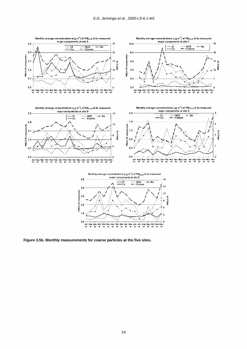
S.G. Jennings et al., 2000-LS-6.1-M1
Figure 3.5b. Monthly measurements for coarse particles at the five sites.
24

Nature and origin of PM10 and smaller particulate matter in urban air
4 Measurements over an Intensive Period
Intensive measurements were carried out during 4 weeks
in February–March 2002 (19 February–21 March) at three
stations: Killure, Ahascragh, Ballinasloe (rural site D),
Coleraine Street (Dublin site B) and Wicklow (coastal site
C). The main objectives of the intensive campaign were to
obtain a greater understanding of pollution sources, of
their strength and impact on air quality and to obtain size-
resolved particle chemical composition measurements in
order to assign accurate size distributions to the major
source categories. The following additional
measurements were carried out:
• condensation particle concentration (CPC) – total
number of particles larger than 10 nm in size;
• SO2, NO, NO2, NOx, O3, CO gas measurements;
• cascade impactor (MOUDI) for collection and
analysis of size-resolved aerosol particles (12 size
categories);
• meteorological data: temperature, wind speed and
direction, relative humidity.
Gaseous measurements were made with 5-min time
resolution, while MOUDI impactor samples were changed
weekly. MOUDI impactors are capable of collecting
particles in up to 12 size fractions within the range 0.054–
18 µm. A 12-stage MOUDI was used at Sites B and D,
whereas at Site C a 10-stage MOUDI was employed. The
10-stage MOUDI is essentially the same as the other two,
but is missing the two smallest particle stages. Those
smallest particles (<0.054 µm) were collected on the
backup filter. MOUDI samples were first weighted
gravimetrically, and then analysed for MSA–, Cl–, Mg2+,
NO3–, SO4
2–, Na+, NH4+, K+, Ca2+ and EC. Analytical
procedures used were the same as those used for the
ordinary samples (Section 2.2).
4.1 Local Meteorology during theIntensive Campaign
Regional meteorology during the intensive campaign was
characterised by a westerly air flow from the Atlantic
Ocean during the first 2 weeks and by an easterly flow at
the end of the campaign. Westerly air flow brings the
cleanest air into Ireland, while the easterly flow brings
polluted air masses from the United Kingdom and
continental Europe. The frequency distribution pattern of
local wind direction throughout the campaign at Sites C
and D is presented in Fig. 4.1. The meteorological
situation was rather stable during the individual 4 weeks
and therefore enabled estimation of the influence of air
masses passing over Ireland from the west and from the
east on pollutant levels in Ireland.
Other meteorological parameters (temperature, relative
humidity and wind speed) were mostly affected by
regional meteorology. The temperature at the rural site
Figure 4.1. Frequency distribution pattern of local wind direction during the intensive campaign measured at the
rural site (D) (left) and Site C (right).
25

S.G. Jennings et al., 2000-LS-6.1-M1
was about a factor of 2 lower than that at the coastal site,
where the warm sea water made temperature
independent of the influence of air masses. The
temperature at the rural site was at its lowest in northerly
air masses and highest in the westerly air masses.
Relative humidity was directly related to the temperature,
with relative humidity values of between 60 and 80% at
the rural site and between 40 and 60% at the coastal site.
Wind speed was variable between 1 and 6 m/s on
average, with a stronger variation at the rural site.
Strongest winds appeared from the western sector, while
the weakest winds generally came from the eastern
sector. Meteorology at the Dublin site (Site B) had strong
local character, affected by street canyons. Wind speed
was very low, generally below 1 m/s, and therefore
measured wind direction was not reliable. Due in part to
the low wind speed, local temperature was rather high,
above 15°C on the average, and relative humidity was
around 40%.
4.2 Gaseous Measurements andCondensation Particle Counts duringthe Intensive Campaign
High-resolution gas measurements enabled estimation of
the strength and impact of local and regional pollution
sources on regional air quality. Figure 4.2 presents
frequency distribution patterns of SO2, NO, NO2 and CPC
counts at Site D during the intensive campaign. NO is a
short-lived gas and it clearly shows the influence of the
nearby sources. Elevated NO concentrations come from
an easterly (around 100°) direction, where Ballinasloe
town, with a population of about 6500 inhabitants, is
situated at a distance of 5–6 km. NO2 concentration does
not follow the same pattern, as NO2 is a photochemical
product of NO, exhibiting a uniform concentration pattern
produced by distant regional sources. The SO2
concentration pattern reveals both local and regional
sources, with slightly elevated concentrations from the
eastern sector. SO2 comes mainly from fossil fuel, mainly
Figure 4.2. Frequency distribution of gases NO, NO2, SO2 and condensation particle concentration (CPC)
measured during the intensive campaign at the rural site (D).
26

Nature and origin of PM10 and smaller particulate matter in urban air
exhibiting influences of nearby sources (Ballinasloe and
Athlone towns) and distant sources (Ireland, the United
Kingdom and the rest of Europe). Gaseous
measurements have shown that Site D is clearly rural and
nearby local pollution sources had little impact on air
quality. Despite clear concentration patterns in some
cases, gaseous concentrations were generally very low
(Table 4.1). CPC counts showed even more pronounced
regional pollution with elevated counts for the north-
eastern sector. It should be pointed out that the CPC
pattern did not show a clear influence of the nearby town,
Ballinasloe, and therefore it can be assumed that local
sources had little influence on aerosol chemical
composition at Site D. This rural site is certainly
representative of regional background air quality. Note
that pollutant concentrations which appeared in the
western sector were generally low, e.g. CPC counts were
about 1500 particles/cm3. By comparison, in clean air
masses advecting into Ireland from the Atlantic CPC
counts are below 700 particles/cm3. Therefore, it can be
concluded that emissions from Galway City had a clear,
but fairly limited, influence on the regional air quality due
to the distance of 70 km from the rural site and favourable
mixing conditions at higher wind speeds from the western
sector. However, this conclusion is made based on
concentration levels only. Despite low CPC
concentrations in the western sector, the chemical
composition of particles is different from the one expected
in the clean marine air masses (Section 4.3).
Gaseous concentration patterns at the coastal site (C)
were similar in their nature to those at the rural site, as
shown in Fig. 4.3. Generally, concentrations were very
low, with the lowest values in the western sector. Variation
of SO2 concentration at the coastal site exhibited a local
character, with multiple concentration spikes associated
with local emissions from either burnt domestic fuel or
from ships. The latter emissions were dominating, as they
have appeared from the seaside, but often lasted only for
about 1 h (measurement resolution). Accompanying high
CPC counts, despite supporting the aforementioned local
emissions, may also have been coming from new particle
formation events at the coast. CPC concentrations in the
western sector were very similar, though slightly higher
than at the rural site, implying that emissions during air
mass passage over Ireland slightly enhanced particle
concentration by about 20–25%. However, NOx and SO2
concentrations remained at a very low level in that sector.
The Dublin site (B) represented a background urban site
with a local meteorology determined by a street canyon.
Gaseous concentrations were not particularly high, as
shown in Fig. 4.4, as the 95th percentile concentration did
not come close to any limit value (Table 4.1). However,
frequency distribution patterns revealed clear pollution
sources. NO, NO2 and CO emissions were advecting
mainly from a southern direction where a busy North King
Street is situated. SO2 emissions did not follow that
pattern, suggesting that urban emissions were coming
mainly from domestic fuel consumption. Elevated SO2
concentration in the south-eastern sector pointed to ship
Table 4.1. Summary of gaseous and CPC concentrations measured during the intensive cam paign (19 Feb 200 2–21 Mar 2002) at Sites B, C and D.Site CO
ppmNOxppb
NO2ppb
NOppb
SO2ppb
O3ppm
CPCparticles/cm3
B (Dublin)
Average 0.44 34.9 14.6 20.2 1.52 na 25,689
5th percentile 0.20 3.00 2.90 0.40 0.40 na 30
95th percentile 0.90 84.6 44.9 40.2 3.80 na 55,550
C (coastal)
Average 0.21 1.77 1.58 0.19 0.48 30.3 2,981
5th percentile 0.04 –0.20 –0.20 –0.28 –0.07 21 419
95th percentile 0.31 6.94 6.30 0.95 1.46 39 11061
D (rural)
Average na 2.81 1.46 1.35 0.81 na 3024
5th percentile na 1.49 0.57 0.17 0.36 na 360
95th percentile na 5.57 2.34 3.91 1.53 na 9266
na: data not available.
27
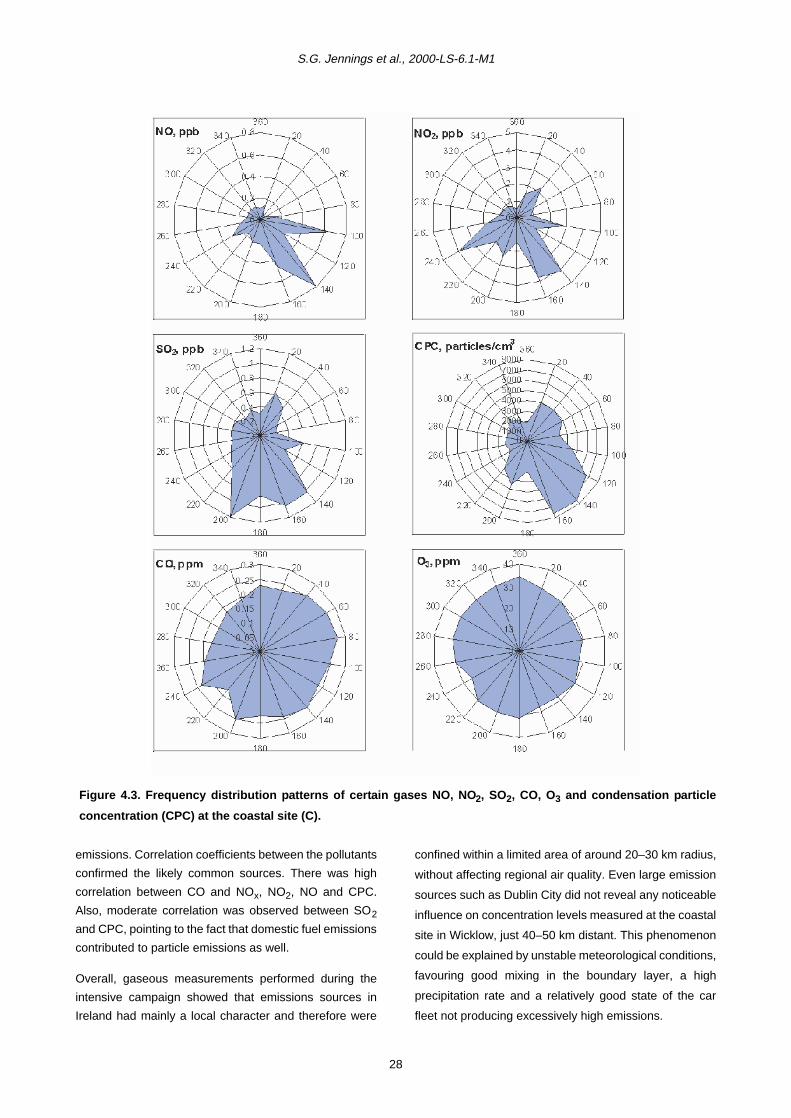
S.G. Jennings et al., 2000-LS-6.1-M1
emissions. Correlation coefficients between the pollutants
confirmed the likely common sources. There was high
correlation between CO and NOx, NO2, NO and CPC.
Also, moderate correlation was observed between SO2
and CPC, pointing to the fact that domestic fuel emissions
contributed to particle emissions as well.
Overall, gaseous measurements performed during the
intensive campaign showed that emissions sources in
Ireland had mainly a local character and therefore were
confined within a limited area of around 20–30 km radius,
without affecting regional air quality. Even large emission
sources such as Dublin City did not reveal any noticeable
influence on concentration levels measured at the coastal
site in Wicklow, just 40–50 km distant. This phenomenon
could be explained by unstable meteorological conditions,
favouring good mixing in the boundary layer, a high
precipitation rate and a relatively good state of the car
fleet not producing excessively high emissions.
Figure 4.3. Frequency distribution patterns of certain gases NO, NO2, SO2, CO, O3 and condensation particle
concentration (CPC) at the coastal site (C).
28
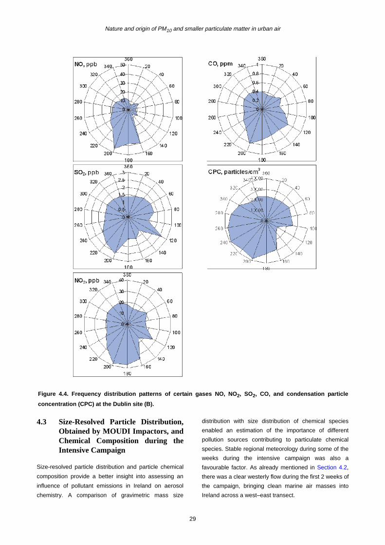
Nature and origin of PM10 and smaller particulate matter in urban air
4.3 Size-Resolved Particle Distribution,Obtained by MOUDI Impactors, andChemical Composition during theIntensive Campaign
Size-resolved particle distribution and particle chemical
composition provide a better insight into assessing an
influence of pollutant emissions in Ireland on aerosol
chemistry. A comparison of gravimetric mass size
distribution with size distribution of chemical species
enabled an estimation of the importance of different
pollution sources contributing to particulate chemical
species. Stable regional meteorology during some of the
weeks during the intensive campaign was also a
favourable factor. As already mentioned in Section 4.2,
there was a clear westerly flow during the first 2 weeks of
the campaign, bringing clean marine air masses into
Ireland across a west–east transect.
Figure 4.4. Frequency distribution patterns of certain gases NO, NO2, SO2, CO, and condensation particle
concentration (CPC) at the Dublin site (B).
29

S.G. Jennings et al., 2000-LS-6.1-M1
Size-resolved gravimetric mass distribution showed clear
differences between particle modes at the three sites. A
demarcation between accumulation and coarse modes
was at about 0.8 µm and was constant at all sites, as
shown in Fig. 4.5. This finding places a new perspective
on the value which is frequently used to separate fine and
coarse particle modes – that of 2.5 µm. Note that the
demarcation size of 0.8 µm represents a ‘wet’ diameter,
as MOUDI impactors were run at ambient temperature.
Therefore, the measurements suggest that dichotomous
samplers should separate particles at a standard 1.0-µm
size, at least under Irish conditions with a strong primary
sea salt source.
An accumulation mode (between particle size diameter
range from 0.1 to 1.0 µm) or fine particle mode mass was
fairly similar at the rural and the coastal sites, while at the
urban background site fine particle mass concentration
was a factor of about 2 to 4 higher due to urban emissions.
The accumulation mode concentration was very different
depending on air mass history, which was factor of 2 to 3
higher in easterly air masses compared to the westerly
ones. The exception was the Coleraine Street site (Site
B), where the accumulation mode concentration was
stable and fairly independent of the air mass sector. This
pointed to the fact that particle mass was dominated by
urban emissions, with only a relatively small difference
attributed to air mass history.
The coarse particle mode was also characteristic of the
different sites. The coarse particle mode at the rural site
was dominated by sea salt particles of about 2 µm in size,
while larger particles were washed out or deposited
before reaching the site. At the coastal site (C), coarse
mode particle mass was dominated by particles of 5–8 µm
in size and was quite dependent on the wind direction,
with a factor of 2 to 3 higher mass during the week of
easterly air flow compared to the westerly flow. Coarse
mode particle mass at the Coleraine Street site exhibited
moderate variation depending on the wind direction, but
much less than at the coastal site.
Chemical species contributing to the measured aerosol
mass are presented in Figs 4.6–4.8 for Sites D, B and C.
There is a clear size demarcation where particle chemical
composition completely changes its distribution pattern.
Particles up to 1.0 µm in size are predominantly
composed of EC, nss SO42– (non-sea-salt sulphate),
NO3– and NH4
+. Particles above 1.0 µm are almost
entirely composed of sea salt (NaCl, ss SO42– (sea-salt
sulphate), Ca and Mg). There were only two exceptions:
(1) at the rural site when due to the strong westerly winds
during the first week of the campaign sea salt significantly
contributed to even the 0.56- to 1.0-µm size range; and (2)
at the urban background site, where Ca significantly
contributed to the coarse mode due to resuspended road
dust. The clear difference in chemical composition, which
occurred at the 1.0-µm size, supports the critics of the 2.5-
µm cut-off size utilised in dichotomous samplers.
On average, all chemical species concentrations
measured in the size-resolved samples were very similar
to the ones measured in the PM10 or PM2.5 samples. Due
to the effect of road traffic, substantial elevations of EC
concentrations were recorded at the Coleraine Street site
(Dublin) in comparison with the rural or coastal
background sites, which were up to 10 times the
Figure 4.5. Particle mass size distributions for the
rural site (D), the city site (B) and the coastal site (C).
30

Nature and origin of PM10 and smaller particulate matter in urban air
Figure 4.6. Mass fraction of aerosol chemical species as a function of particle size at the rural site (D).
31

S.G. Jennings et al., 2000-LS-6.1-M1
concentrations at the other two sites. Consequently, EC
concentration at the Coleraine Street site accounted for
up to 90% of the particle mass in the size range of 0.1–
0.2 µm. As EC comes primarily from burned fossil fuel it
has a strong local character. There were much less
differences between other chemical species at the
different sites. Non-sea-salt SO42– concentrations were
only up to 50% higher at the urban site compared to the
rural or coastal site, while NO3– and NH4
+ concentrations
were similar at the urban and coastal sites, but a factor of
2 to 3 higher than at the rural site. The only unusual
finding was a noticeable contribution of calcium to the
smallest sized particles at all sites.
Constant westerly air flow during the first week of the
intensive campaign provided us with an insight into the
influence of pollution sources in Ireland on aerosol
chemical composition. Figure 4.9 shows an increase in
Figure 4.7. Mass fraction of aerosol chemical species as a function of particle size at the urban site (B).
32

Nature and origin of PM10 and smaller particulate matter in urban air
Figure 4.8. Mass fraction of aerosol chemical species as a function of particle size at the coastal site (C).
33
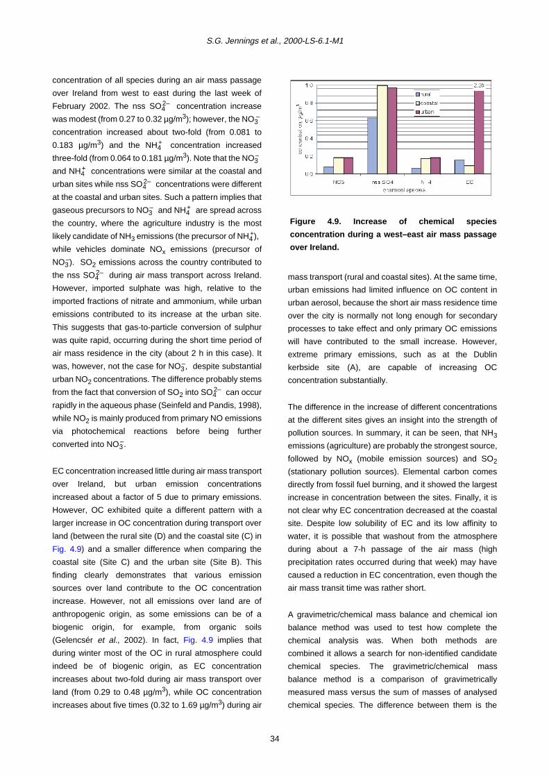
S.G. Jennings et al., 2000-LS-6.1-M1
concentration of all species during an air mass passage
over Ireland from west to east during the last week of
February 2002. The nss SO42– concentration increase
was modest (from 0.27 to 0.32 µg/m3); however, the NO3–
concentration increased about two-fold (from 0.081 to
0.183 µg/m3) and the NH4+ concentration increased
three-fold (from 0.064 to 0.181 µg/m3). Note that the NO3–
and NH4+ concentrations were similar at the coastal and
urban sites while nss SO42– concentrations were different
at the coastal and urban sites. Such a pattern implies that
gaseous precursors to NO3– and NH4
+ are spread across
the country, where the agriculture industry is the most
likely candidate of NH3 emissions (the precursor of NH4+),
while vehicles dominate NOx emissions (precursor of
NO3–). SO2 emissions across the country contributed to
the nss SO42– during air mass transport across Ireland.
However, imported sulphate was high, relative to the
imported fractions of nitrate and ammonium, while urban
emissions contributed to its increase at the urban site.
This suggests that gas-to-particle conversion of sulphur
was quite rapid, occurring during the short time period of
air mass residence in the city (about 2 h in this case). It
was, however, not the case for NO3–, despite substantial
urban NO2 concentrations. The difference probably stems
from the fact that conversion of SO2 into SO42– can occur
rapidly in the aqueous phase (Seinfeld and Pandis, 1998),
while NO2 is mainly produced from primary NO emissions
via photochemical reactions before being further
converted into NO3–.
EC concentration increased little during air mass transport
over Ireland, but urban emission concentrations
increased about a factor of 5 due to primary emissions.
However, OC exhibited quite a different pattern with a
larger increase in OC concentration during transport over
land (between the rural site (D) and the coastal site (C) in
Fig. 4.9) and a smaller difference when comparing the
coastal site (Site C) and the urban site (Site B). This
finding clearly demonstrates that various emission
sources over land contribute to the OC concentration
increase. However, not all emissions over land are of
anthropogenic origin, as some emissions can be of a
biogenic origin, for example, from organic soils
(Gelencsér et al., 2002). In fact, Fig. 4.9 implies that
during winter most of the OC in rural atmosphere could
indeed be of biogenic origin, as EC concentration
increases about two-fold during air mass transport over
land (from 0.29 to 0.48 µg/m3), while OC concentration
increases about five times (0.32 to 1.69 µg/m3) during air
mass transport (rural and coastal sites). At the same time,
urban emissions had limited influence on OC content in
urban aerosol, because the short air mass residence time
over the city is normally not long enough for secondary
processes to take effect and only primary OC emissions
will have contributed to the small increase. However,
extreme primary emissions, such as at the Dublin
kerbside site (A), are capable of increasing OC
concentration substantially.
The difference in the increase of different concentrations
at the different sites gives an insight into the strength of
pollution sources. In summary, it can be seen, that NH3
emissions (agriculture) are probably the strongest source,
followed by NOx (mobile emission sources) and SO2
(stationary pollution sources). Elemental carbon comes
directly from fossil fuel burning, and it showed the largest
increase in concentration between the sites. Finally, it is
not clear why EC concentration decreased at the coastal
site. Despite low solubility of EC and its low affinity to
water, it is possible that washout from the atmosphere
during about a 7-h passage of the air mass (high
precipitation rates occurred during that week) may have
caused a reduction in EC concentration, even though the
air mass transit time was rather short.
A gravimetric/chemical mass balance and chemical ion
balance method was used to test how complete the
chemical analysis was. When both methods are
combined it allows a search for non-identified candidate
chemical species. The gravimetric/chemical mass
balance method is a comparison of gravimetrically
measured mass versus the sum of masses of analysed
chemical species. The difference between them is the
Figure 4.9. Increase of chemical species
concentration during a west–east air mass passage
over Ireland.
34

Nature and origin of PM10 and smaller particulate matter in urban air
unresolved mass. Figure 4.10 presents gravimetric mass
balance at the three sites. Overall, the best balance was
achieved at the Coleraine Street site; the worst was at the
rural site, where unresolved mass accounted for up to
90% for certain particle sizes. All major chemical
components, representing major pollutants, were
analysed at all sites. However, as the Coleraine Street site
was the most polluted one, main pollutants such as EC
accounted for the major mass fraction, thus improving the
mass balance. At the relatively clean rural site, mass
deficiency was very significant. It is thought that the
majority of the missing mass in the fine fraction could be
attributed to the non-analysed OC, which is present in
significant amounts in all air masses. Organic carbon can
be produced by primary as well as secondary processes,
and therefore is present at all sites. In summary, organic
emissions contributing to unresolved mass could be of
biogenic origin, either from marine sources (O’Dowd et al.,
2004) or from continental soils (Gelencsér et al., 2002).
Some organic emissions could also be due to
anthropogenic sources.
The ion balance method, which is the ratio of positive and
negative ions, can give further insight into missing
chemical species. Figure 4.11 shows chemical ion
balance at the three sites. Deficiency in negative ions
across small particle sizes confirms that non-analysed
organic acids could be responsible for the missing mass.
There was also missing mass across large particle sizes.
In this case, the mass balance and ion balance method
suggest that the missing candidate species could be crust
material, particularly silicates and carbonates, providing
large sources of negative ions. Note that at the coastal
site there was little missing mass across large particle
sizes and there was rather good ion balance due to the
Figure 4.10. Gravimetric mass distributions at the
rural, city and coastal sites.
Figure 4.11. Chemical ion balance at the rural, city
and coastal sites.
35
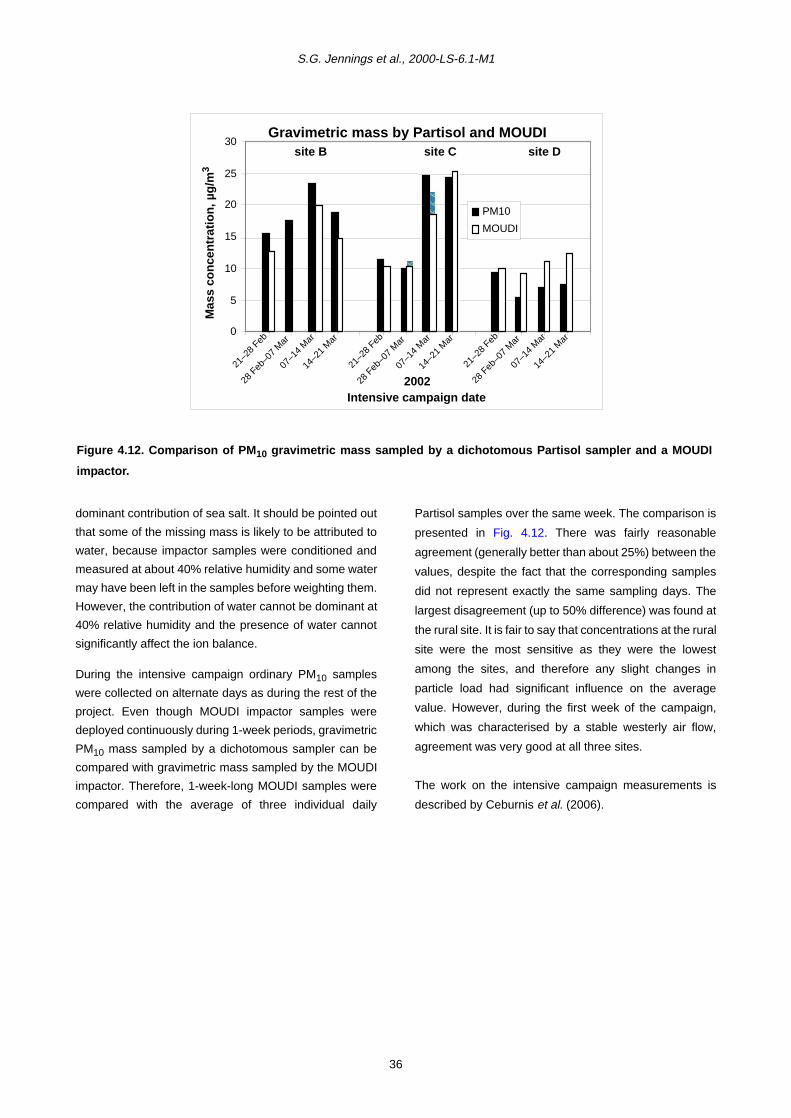
S.G. Jennings et al., 2000-LS-6.1-M1
dominant contribution of sea salt. It should be pointed out
that some of the missing mass is likely to be attributed to
water, because impactor samples were conditioned and
measured at about 40% relative humidity and some water
may have been left in the samples before weighting them.
However, the contribution of water cannot be dominant at
40% relative humidity and the presence of water cannot
significantly affect the ion balance.
During the intensive campaign ordinary PM10 samples
were collected on alternate days as during the rest of the
project. Even though MOUDI impactor samples were
deployed continuously during 1-week periods, gravimetric
PM10 mass sampled by a dichotomous sampler can be
compared with gravimetric mass sampled by the MOUDI
impactor. Therefore, 1-week-long MOUDI samples were
compared with the average of three individual daily
Partisol samples over the same week. The comparison is
presented in Fig. 4.12. There was fairly reasonable
agreement (generally better than about 25%) between the
values, despite the fact that the corresponding samples
did not represent exactly the same sampling days. The
largest disagreement (up to 50% difference) was found at
the rural site. It is fair to say that concentrations at the rural
site were the most sensitive as they were the lowest
among the sites, and therefore any slight changes in
particle load had significant influence on the average
value. However, during the first week of the campaign,
which was characterised by a stable westerly air flow,
agreement was very good at all three sites.
The work on the intensive campaign measurements is
described by Ceburnis et al. (2006).
Figure 4.12. Comparison of PM10 gravimetric mass sampled by a dichotomous Partisol sampler and a MOUDI
impactor.
Gravimetric mass by Partisol and MOUDI
0
5
10
15
20
25
30
Intensive campaign date
PM10
MOUDI
site B site C site D
21–2
8 Feb
28 F
eb–0
7 M
ar
07–1
4 M
ar
14–2
1 M
ar
21–2
8 Feb
28 F
eb–0
7 M
ar
07–1
4 M
ar
14–2
1 M
ar
21–2
8 Feb
28 F
eb–0
7 M
ar
07–1
4 M
ar
14–2
1 M
ar
2002
Mas
s co
nce
ntr
atio
n, µ
g/m
3
36

Nature and origin of PM10 and smaller particulate matter in urban air
5 PM10 Episodes Study and Air Mass Back-TrajectoryAnalyses
Urban sites are most likely to exceed the PM10 standard
limit 24-hour mean value of 50 µg/m3, particularly at
heavily trafficked locations. Closer examination of
selected days when PM10 exceeded the standard limit
has been conducted considering particle physical and
chemical properties, and meteorology. Air mass back
trajectories were obtained using the British Atmospheric
Data Centre (BADC) trajectory service to aid in
interpretation of the data.
5.1 Relative Importance of Fine andCoarse Particles and their ChemicalComposition during PM10 Episodes
Figure 5.1 shows the proportions of fine and coarse
particles contributing to the total concentrations of PM10
on days when PM10 mass exceeded 50 µg/m3. At urban
sites A, B and E, PM10 episodes were mostly dominated
by the fine fraction, which contributes 62% (range: 30–
89%) of the PM10 mass on average at Site A, 74% (range:
63–89%) at site B and 67% (range: 43–83%) at Site E.
The coarse fraction was predominant only on a few
occasions (5 days) at Site A, but its contribution is not
negligible, making up about one-third of the total mass,
largely due to resuspension of dusts by heavy traffic, as
evidenced by high concentrations of calcium (Fig. 5.2).
Sea salt may make a large contribution at this site (A)
(11/12/02) but on very rare occasions. In comparison, Site
E is less influenced by dust resuspension because of a
lower traffic volume and the higher position above the
ground of the sampling inlet; however, there were also 2
days (12/12/01 and 18/09/02) when over 50% of PM10
mass was from coarse particles, which mainly comprised
resuspended dusts, sea salt and nitrate. Similarly, Site B
experienced less traffic activity than Site A, and during
almost all PM10 episodes the total mass consisted of more
than two-thirds of fine particles. There were only 5 days at
Site C that PM10 exceeded the EU limit, but on 2 days the
coarse fraction was predominant, contributing about 75%
and 78%, almost purely due to sea salt. The only day
recorded when PM10 was over the standard limit at Site D
showed an 80% contribution from fine particles.
5.2 Use of Air Mass Back Trajectories inAnalysis of PM10 Episodes
Meteorological data (wind speed, wind direction, ambient
temperature, pressure and relative humidity) were
downloaded from the Partisol instruments at Sites A, B
and C with only poor data capture (about 30%). Wind data
are only available for the period June 2002 to December
2002 at Site E and from October 2001 to December 2002
at Site D. These were not used due to the short run of data
(although a reasonably high data capture was obtained at
Site D). Instead, 5-day air mass back trajectories were
obtained using the BADC trajectory service, and used to
identify the likely influences of different air mass/aerosol
origins, whether local, regional, national, European or
North Atlantic. In the following section, different air mass
origins are illustrated, together with analysis of the 24-h
particle mass and chemical component mass for selected
days characterised by the presence of both polluted and
clean air masses.
Example 1
On 15 August 2001 the air mass followed an Atlantic
trajectory, crossing south-east Ireland before reaching the
sites, with no signs of a European influence (Fig. 5.3a).
The local wind direction was consistent with the trajectory
at around 205°. High PM10 mass (88 µg/m3) was recorded
at Site A, comprising about 60% from the coarse fraction
largely due to high levels of resuspended materials
indicated by an elevated calcium concentration of about 9
µg/m3. The EC concentration was also high on this day,
again indicating a local traffic source of emissions. Low
secondary aerosol mass was measured. In comparison,
Site B exhibited much lower PM10 mass concentration (16
µg/m3), although also composed of a higher proportion of
coarse particles. A similar profile was found as at Site A,
with higher calcium and EC, and lower secondary
component levels. On this day local sources
predominated in an air mass originating over the Atlantic.
Example 2
The highest PM10 concentrations measured over the
whole sampling period occurred on 12 December 2001 at
Site A (161 µg/m3) and at Site B (106 µg/m3) (Fig. 5.3b).
37

S.G. Jennings et al., 2000-LS-6.1-M1
Figure 5.1. Daily fine and coarse mass concentrations when PM10 >50 µg/m 3.
PM 10 concentrations over 50 µ g m -3 at site B
0
11
22
33
44
55
66
77
88
99
110
08/1
2/0
1
12/1
2/0
1
01/0
1/0
2
05/0
1/0
2
07/0
1/0
2
09/0
1/0
2
28/0
3/0
2
30/0
3/0
2
05/0
4/0
2
11/0
4/0
2
12/0
9/0
2
Fine Coarse
PM 10 concentrations over 50 µ g m -3 at site A
0
33
66
99
132
165
25
/07
/01
17
/08
/01
29
/08
/01
21
/09
/01
14
/11
/01
18
/11
/01
08
/12
/01
12
/12
/01
18
/12
/01
01
/01
/02
07
/01
/02
11
/01
/02
12
/03
/02
28
/03
/02
05
/04
/02
11
/04
/02
01
/08
/02
12
/09
/02
24
/09
/02
18
/10
/02
05
/11
/02
03
/12
/02
11
/12
/02
17
/12
/02
Fine Coa rse
PM10 concentrations over 50 µ g m -3 at site E
0
11
22
33
44
55
66
77
88
99
110
21/0
9/0
1
14/1
1/0
1
22/1
1/0
1
12/1
2/0
1
05/0
1/0
2
09/0
1/0
2
17/0
1/0
2
28/0
3/0
2
05/0
4/0
2
18/0
9/0
2
29/1
1/0
2
05/1
2/0
2
11/1
2/0
2
13/1
2/0
2
15/1
2/0
2
Fine Coarse
PM10 concentrations over 50 µ g m -3 at site C & D
0
20
40
60
80
C-0
3/0
1/0
2
30
/03
/02
05
/04
/02
12
/09
/02
19
/12
/02
D-0
5/0
4/0
2
Fine Coarse
38
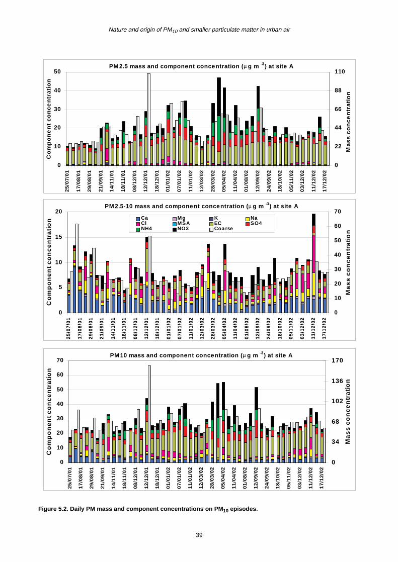
Nature and origin of PM10 and smaller particulate matter in urban air
Figure 5.2. Daily PM mass and component concentrations on PM10 episodes.
PM2.5 mass and component concentration (µ g m -3) at site A
0
10
20
30
40
502
5/0
7/0
1
17
/08
/01
29
/08
/01
21
/09
/01
14
/11
/01
18
/11
/01
08
/12
/01
12
/12
/01
18
/12
/01
01
/01
/02
07
/01
/02
11
/01
/02
12
/03
/02
28
/03
/02
05
/04
/02
11
/04
/02
01
/08
/02
12
/09
/02
24
/09
/02
18
/10
/02
05
/11
/02
03
/12
/02
11
/12
/02
17
/12
/02
Co
mp
on
en
t c
on
cen
trat
ion
0
22
44
66
88
110
Ma
ss
co
nce
ntr
ati
on
PM2.5-10 mass and component concentration (µ g m -3) at site A
0
5
10
15
20
25
/07
/01
17
/08
/01
29
/08
/01
21
/09
/01
14
/11
/01
18
/11
/01
08
/12
/01
12
/12
/01
18
/12
/01
01
/01
/02
07
/01
/02
11
/01
/02
12
/03
/02
28
/03
/02
05
/04
/02
11
/04
/02
01
/08
/02
12
/09
/02
24
/09
/02
18
/10
/02
05
/11
/02
03
/12
/02
11
/12
/02
17
/12
/02
Co
mp
on
en
t c
on
ce
ntr
ati
on
0
10
20
30
40
50
60
70
Ma
ss
co
nc
en
tra
tio
n
Ca Mg K NaCl MSA EC SO4NH4 NO3 Coarse
PM10 mass and component concentration (µ g m -3) at site A
0
10
20
30
40
50
60
70
25
/07
/01
17
/08
/01
29
/08
/01
21
/09
/01
14
/11
/01
18
/11
/01
08
/12
/01
12
/12
/01
18
/12
/01
01
/01
/02
07
/01
/02
11
/01
/02
12
/03
/02
28
/03
/02
05
/04
/02
11
/04
/02
01
/08
/02
12
/09
/02
24
/09
/02
18
/10
/02
05
/11
/02
03
/12
/02
11
/12
/02
17
/12
/02
Co
mp
on
en
t c
on
ce
ntr
ati
on
0
34
68
102
136
170
Ma
ss
co
nc
en
tra
tio
n
39
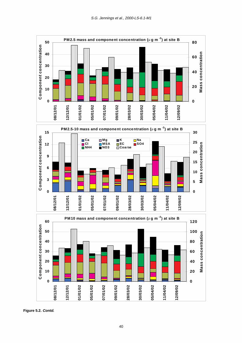
S.G. Jennings et al., 2000-LS-6.1-M1
Figure 5.2. Contd.
PM2.5 mass and component concentration (µ g m -3) at site B
0
10
20
30
40
50
08/1
2/0
1
12/1
2/0
1
01/0
1/0
2
05/0
1/0
2
07/0
1/0
2
09/0
1/0
2
28/0
3/0
2
30/0
3/0
2
05/0
4/0
2
11/0
4/0
2
12/0
9/0
2
Co
mp
on
en
t c
on
ce
ntr
ati
on
0
20
40
60
80
Ma
ss
co
nc
en
tra
tio
n
PM2.5-10 mass and component concentration (µ g m -3) at site B
0
3
6
9
12
15
08/1
2/01
12/1
2/01
01/0
1/02
05/0
1/02
07/0
1/02
09/0
1/02
28/0
3/02
30/0
3/02
05/0
4/02
11/0
4/02
12/0
9/02
Co
mp
on
en
t c
on
ce
ntr
ati
on
0
5
10
15
20
25
30
Ma
ss
co
nc
en
tra
tio
n
Ca Mg K NaCl MSA EC SO4NH4 NO3 Coarse
PM10 mass and component concentration (µ g m -3) at site B
0
10
20
30
40
50
60
08/1
2/0
1
12/1
2/0
1
01/0
1/0
2
05/0
1/0
2
07/0
1/0
2
09/0
1/0
2
28/0
3/0
2
30/0
3/0
2
05/0
4/0
2
11/0
4/0
2
12/0
9/0
2
Co
mp
on
en
t c
on
ce
ntr
ati
on
0
20
40
60
80
100
120
Ma
ss
co
nc
en
tra
tio
n
40
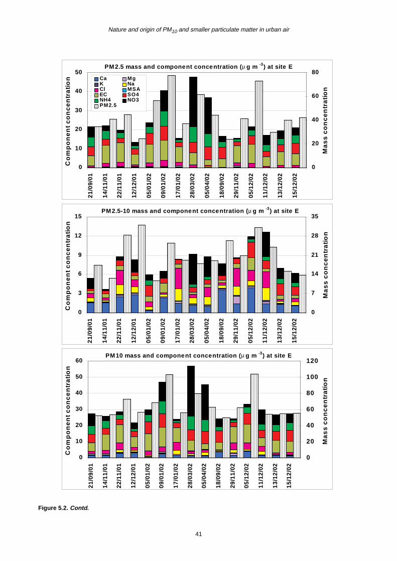
Nature and origin of PM10 and smaller particulate matter in urban air
Figure 5.2. Contd.
PM2.5 mass and component concentration (µ g m -3) at site E
0
10
20
30
40
50
21/0
9/01
14/1
1/01
22/1
1/01
12/1
2/01
05/0
1/02
09/0
1/02
17/0
1/02
28/0
3/02
05/0
4/02
18/0
9/02
29/1
1/02
05/1
2/02
11/1
2/02
13/1
2/02
15/1
2/02
Co
mp
on
en
t c
on
ce
ntr
ati
on
0
20
40
60
80
Ma
ss
co
nc
en
tra
tio
n
Ca MgK NaCl MSAEC SO4NH4 NO3PM2.5
PM2.5-10 mass and component concentration (µ g m -3) at site E
0
3
6
9
12
15
21/
09/
01
14/
11/
01
22/
11/
01
12/
12/
01
05/
01/
02
09/
01/
02
17/
01/
02
28/
03/
02
05/
04/
02
18/
09/
02
29/
11/
02
05/
12/
02
11/
12/
02
13/
12/
02
15/
12/
02
Co
mp
on
en
t c
on
ce
ntr
ati
on
0
7
14
21
28
35
Ma
ss
co
nc
en
tra
tio
n
PM10 mass and component concentration (µ g m -3) at site E
0
10
20
30
40
50
60
21/
09/0
1
14/
11/0
1
22/
11/0
1
12/
12/0
1
05/
01/0
2
09/
01/0
2
17/
01/0
2
28/
03/0
2
05/
04/0
2
18/
09/0
2
29/
11/0
2
05/
12/0
2
11/
12/0
2
13/
12/0
2
15/
12/0
2
Co
mp
on
en
t c
on
ce
ntr
ati
on
0
20
40
60
80
100
120
Ma
ss
co
nc
en
tra
tio
n
41

S.G. Jennings et al., 2000-LS-6.1-M1
Figure 5.2. Contd.
PM2.5 m ass & component concentra tion (µ g m -3) a t site C & D
0
10
20
30
40
50
C-0
3/0
1/0
2
30/0
3/0
2
05/0
4/0
2
12/0
9/0
2
19/1
2/0
2
D-0
5/0
4/0
2
Co
mp
on
en
t c
on
ce
ntr
ati
on
0
10
20
30
40
50
Mas
s c
on
cen
tra
tio
n
PM2.5-10 m ass & component concentra tion (µ g m -3) a t site C & D
0
10
20
30
40
50
30
/03
/02
05
/04
/02
12
/09
/02
19
/12
/02
D-0
5/0
4/0
2
Co
mp
on
en
t c
on
ce
ntr
ati
on
0
10
20
30
40
50
Ma
ss
co
nc
en
tra
tio
nCa Mg K NaCl MSA EC SO4NH4 NO3 Coarse
PM10 m ass & component concentra tion (µ g m -3) a t site C & D
0
10
20
30
40
50
60
C-0
3/0
1/0
2
30
/03
/02
05
/04
/02
12
/09
/02
19
/12
/02
D-0
5/0
4/0
2
Co
mp
on
en
t c
on
ce
ntr
ati
on
0
10
20
30
40
50
60
70
Ma
ss
co
nc
en
tra
tio
n
42
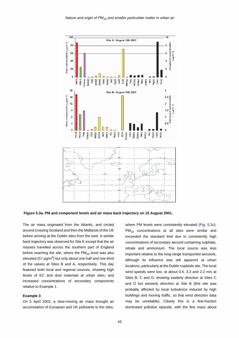
Nature and origin of PM10 and smaller particulate matter in urban air
The air mass originated from the Atlantic, and circled
around crossing Scotland and then the Midlands of the UK
before arriving at the Dublin sites from the east. A similar
back trajectory was observed for Site E except that the air
masses travelled across the southern part of England
before reaching the site, where the PM10 level was also
elevated (57 µg/m3) but only about one-half and one-third
of the values at Sites B and A, respectively. This day
featured both local and regional sources, showing high
levels of EC and dust materials at urban sites, and
increased concentrations of secondary components
relative to Example 1.
Example 3
On 5 April 2002, a slow-moving air mass brought an
accumulation of European and UK pollutants to the sites,
where PM levels were consistently elevated (Fig. 5.3c).
PM10 concentrations at all sites were similar and
exceeded the standard limit due to consistently high
concentrations of secondary aerosol containing sulphate,
nitrate and ammonium. The local source was less
important relative to the long-range transported aerosols,
although its influence was still apparent at urban
locations, particularly at the Dublin roadside site. The local
wind speeds were low, at about 0.4, 3.3 and 2.2 m/s at
Sites B, C and D, showing easterly direction at Sites C
and D but westerly direction at Site B (this site was
probably affected by local turbulence induced by high
buildings and moving traffic, so that wind direction data
may be unreliable). Clearly this is a fine-fraction
dominated pollution episode, with the fine mass about
Figure 5.3a. PM and component levels and air mass back trajectory on 15 August 2001.
43
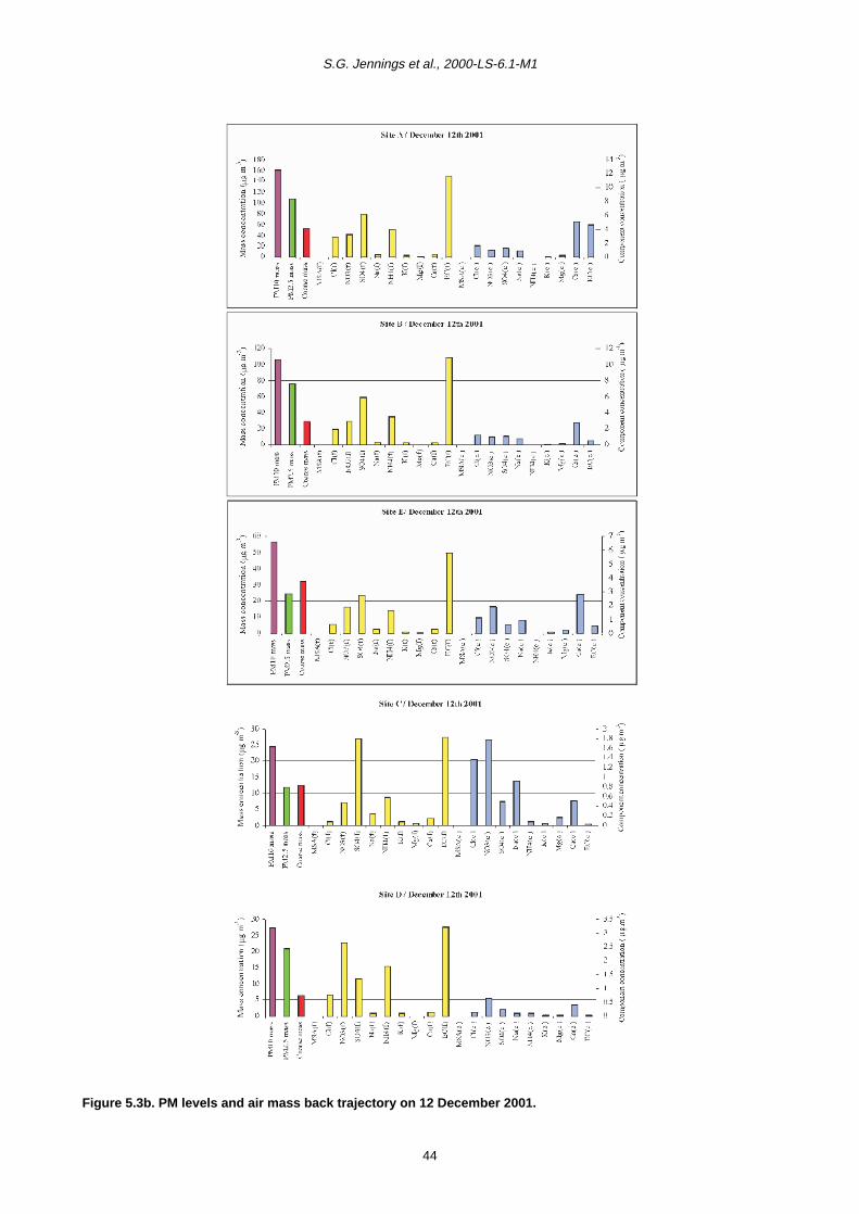
S.G. Jennings et al., 2000-LS-6.1-M1
Figure 5.3b. PM levels and air mass back trajectory on 12 December 2001.
44
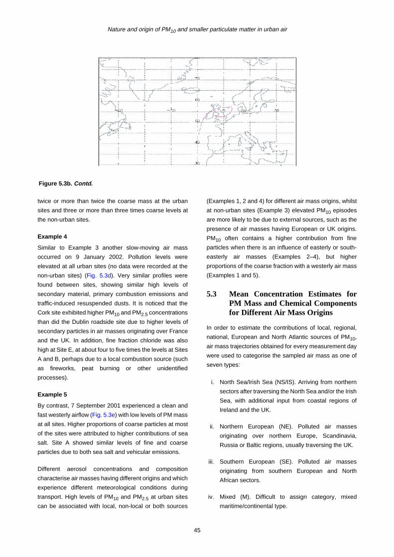
Nature and origin of PM10 and smaller particulate matter in urban air
twice or more than twice the coarse mass at the urban
sites and three or more than three times coarse levels at
the non-urban sites.
Example 4
Similar to Example 3 another slow-moving air mass
occurred on 9 January 2002. Pollution levels were
elevated at all urban sites (no data were recorded at the
non-urban sites) (Fig. 5.3d). Very similar profiles were
found between sites, showing similar high levels of
secondary material, primary combustion emissions and
traffic-induced resuspended dusts. It is noticed that the
Cork site exhibited higher PM10 and PM2.5 concentrations
than did the Dublin roadside site due to higher levels of
secondary particles in air masses originating over France
and the UK. In addition, fine fraction chloride was also
high at Site E, at about four to five times the levels at Sites
A and B, perhaps due to a local combustion source (such
as fireworks, peat burning or other unidentified
processes).
Example 5
By contrast, 7 September 2001 experienced a clean and
fast westerly airflow (Fig. 5.3e) with low levels of PM mass
at all sites. Higher proportions of coarse particles at most
of the sites were attributed to higher contributions of sea
salt. Site A showed similar levels of fine and coarse
particles due to both sea salt and vehicular emissions.
Different aerosol concentrations and composition
characterise air masses having different origins and which
experience different meteorological conditions during
transport. High levels of PM10 and PM2.5 at urban sites
can be associated with local, non-local or both sources
(Examples 1, 2 and 4) for different air mass origins, whilst
at non-urban sites (Example 3) elevated PM10 episodes
are more likely to be due to external sources, such as the
presence of air masses having European or UK origins.
PM10 often contains a higher contribution from fine
particles when there is an influence of easterly or south-
easterly air masses (Examples 2–4), but higher
proportions of the coarse fraction with a westerly air mass
(Examples 1 and 5).
5.3 Mean Concentration Estimates forPM Mass and Chemical Componentsfor Different Air Mass Origins
In order to estimate the contributions of local, regional,
national, European and North Atlantic sources of PM10,
air mass trajectories obtained for every measurement day
were used to categorise the sampled air mass as one of
seven types:
i. North Sea/Irish Sea (NS/IS). Arriving from northern
sectors after traversing the North Sea and/or the Irish
Sea, with additional input from coastal regions of
Ireland and the UK.
ii. Northern European (NE). Polluted air masses
originating over northern Europe, Scandinavia,
Russia or Baltic regions, usually traversing the UK.
iii. Southern European (SE). Polluted air masses
originating from southern European and North
African sectors.
iv. Mixed (M). Difficult to assign category, mixed
maritime/continental type.
Figure 5.3b. Contd.
45

S.G. Jennings et al., 2000-LS-6.1-M1
Figure 5.3c. PM levels and air mass back trajectory on 5 April 2002.
46
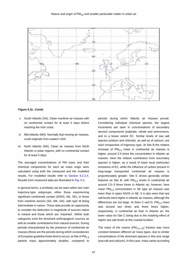
Nature and origin of PM10 and smaller particulate matter in urban air
v. South Atlantic (SA). Clean maritime air masses with
no continental contact for at least 5 days before
reaching the Irish coast.
vi. Mid-Atlantic (MA). Normally fast-moving air masses,
could originate from eastern USA.
vii. North Atlantic (NA). Clean air masses from North
Atlantic or polar regions, with no continental contact
for at least 5 days.
The averaged concentrations of PM mass and their
chemical components for each air mass origin were
calculated using both the measured and the modelled
results. For modelled results refer to Section 6.2.2.4.
Results from measured data are illustrated in Fig. 5.4.
In general terms, a similarity can be seen within two main
trajectory-type subgroups, either those experiencing
significant continental contact (NS/IS, NE, SE), or those
from maritime sectors (SA, MA, NA), with type M being
intermediate in nature. These data provide an opportunity
to consider the distinction in magnitude of sources native
to Ireland and those which are ‘imported’. Within both
categories exist the dominant anthropogenic sources as
well as smaller contributions from natural sources. During
periods characterised by the presence of continental air
masses (these are the periods during which exceedances
of European guideline limits tend to occur), at Site A PM2.5
particle mass approximately doubles, compared to
periods during which Atlantic air masses prevail.
Considering individual chemical species, the largest
increments are seen in concentrations of secondary
aerosol components (sulphate, nitrate and ammonium),
and to a lesser extent EC. Similar levels of sea salt
species (sodium and chloride), as well as of calcium, are
seen irrespective of trajectory type. At Site B the relative
increase of PM2.5 mass in continental air masses is
higher, around 2.5 times the concentration in Atlantic air
masses. Here the relative contribution from secondary
species is higher, as a result of lower local (vehicular)
emissions of EC, while the influence of carbon present in
long-range transported continental air masses is
proportionately greater. Site E shows generally similar
features as Site B, with PM2.5 levels in continental air
around 2.5–3 times those in Atlantic air; however, here
mean PM2.5 concentration in SE type air masses was
lower than in types NS/IS or NE. It is also seen that sea
salt levels were higher in Atlantic air masses, although the
differences are not large. At Sites C and D, PM2.5 mass
was around two times and three times higher,
respectively, in continental air than in Atlantic air, the
lower value for Site C being due to the masking effect of
higher sea salt levels at this coastal location.
The mass of the coarse (PM2.5–10) fraction was more
constant between different air mass types, due to similar
concentrations of the dominant species in this size range
(sea salt and calcium). In this case, mass varies according
Figure 5.3c. Contd.
47
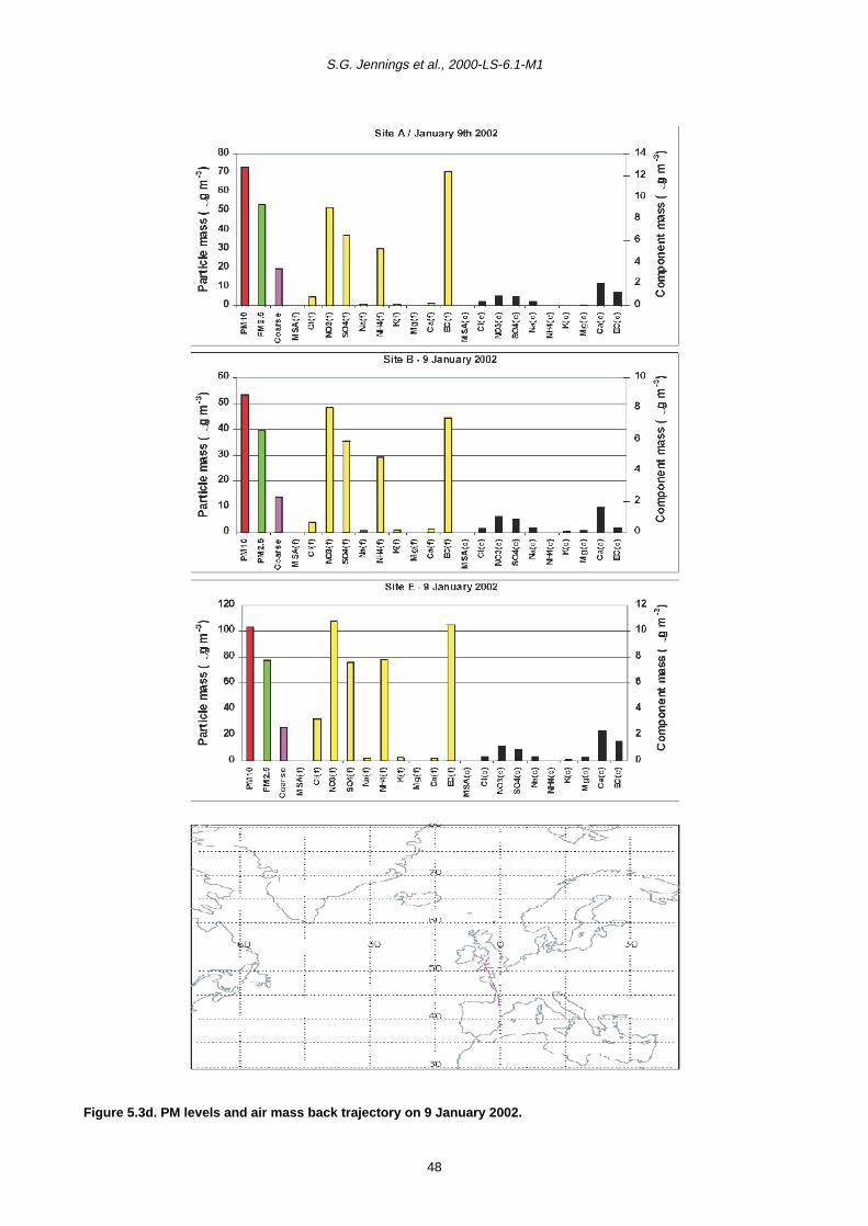
S.G. Jennings et al., 2000-LS-6.1-M1
Figure 5.3d. PM levels and air mass back trajectory on 9 January 2002.
48
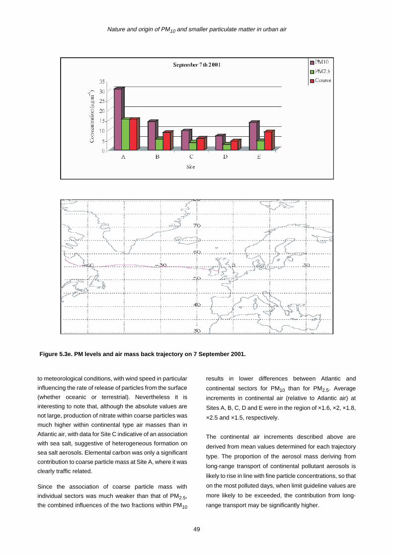
Nature and origin of PM10 and smaller particulate matter in urban air
to meteorological conditions, with wind speed in particular
influencing the rate of release of particles from the surface
(whether oceanic or terrestrial). Nevertheless it is
interesting to note that, although the absolute values are
not large, production of nitrate within coarse particles was
much higher within continental type air masses than in
Atlantic air, with data for Site C indicative of an association
with sea salt, suggestive of heterogeneous formation on
sea salt aerosols. Elemental carbon was only a significant
contribution to coarse particle mass at Site A, where it was
clearly traffic related.
Since the association of coarse particle mass with
individual sectors was much weaker than that of PM2.5,
the combined influences of the two fractions within PM10
results in lower differences between Atlantic and
continental sectors for PM10 than for PM2.5. Average
increments in continental air (relative to Atlantic air) at
Sites A, B, C, D and E were in the region of ×1.6, ×2, ×1.8,
×2.5 and ×1.5, respectively.
The continental air increments described above are
derived from mean values determined for each trajectory
type. The proportion of the aerosol mass deriving from
long-range transport of continental pollutant aerosols is
likely to rise in line with fine particle concentrations, so that
on the most polluted days, when limit guideline values are
more likely to be exceeded, the contribution from long-
range transport may be significantly higher.
Figure 5.3e. PM levels and air mass back trajectory on 7 September 2001.
49
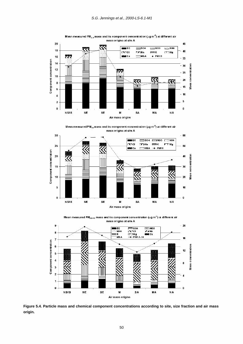
S.G. Jennings et al., 2000-LS-6.1-M1
Figure 5.4. Particle mass and chemical component concentrations according to site, size fraction and air mass
origin.
50

Nature and origin of PM10 and smaller particulate matter in urban air
Figure 5.4. Contd.
51
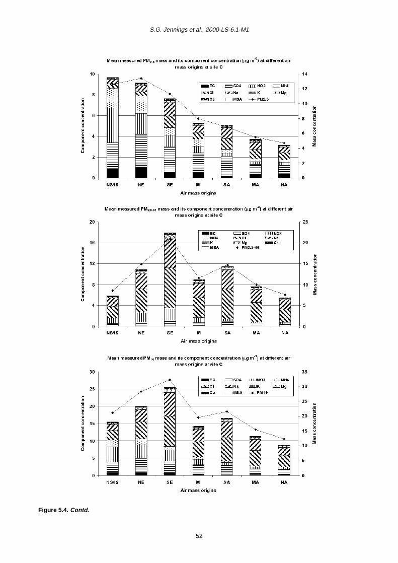
S.G. Jennings et al., 2000-LS-6.1-M1
Figure 5.4. Contd.
52
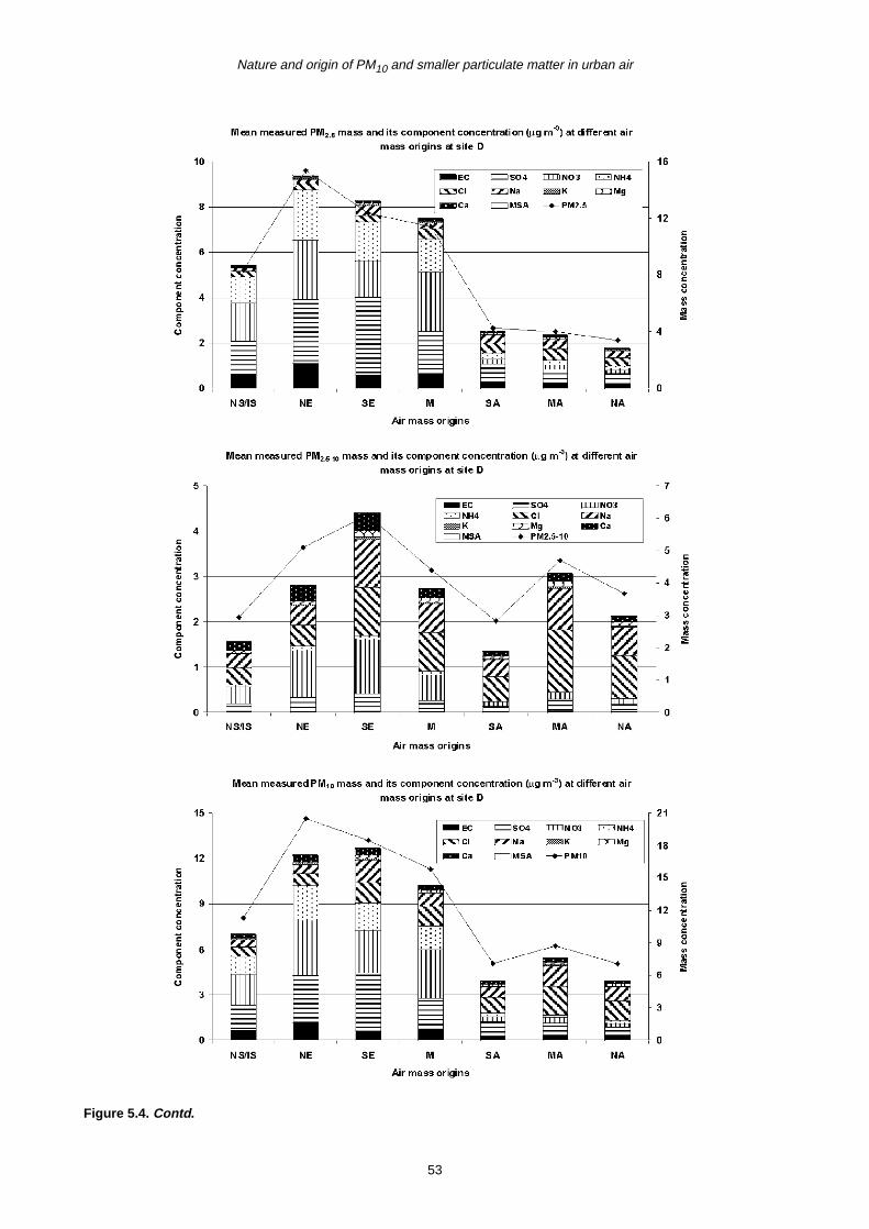
Nature and origin of PM10 and smaller particulate matter in urban air
Figure 5.4. Contd.
53

S.G. Jennings et al., 2000-LS-6.1-M1
Figure 5.4. Contd.
54

Nature and origin of PM10 and smaller particulate matter in urban air
6 Source Apportionment of Aerosol PM10, PM2.5 andPM2.5–10
6.1 PM Source Apportionment Using theChemical Reconstruction Method
6.1.1 Mass closure analysis using measured
chemical componentsMass closure analysis was conducted by comparing the
aerosol gravimetric mass and its measured chemical
components, shown in Fig. 6.1. The measured
components explain a large portion, in the range 38–76%,
of the PM mass, so that chemical component
reconstruction may be usefully employed to evaluate the
aerosol chemical composition and/or pollution sources,
based on the assumption that suitable source/component
markers are employed (discussed in Section 6.1.2). Apart
from the other (unmeasured) component, the major
chemical make-up of PM2.5 at urban sites comprises EC,
sulphate, nitrate and ammonium. A lesser contribution
arises from sea salt and very little from calcium,
potassium, magnesium and MSA. The largest proportion
in coarse particles at urban sites is sea salt, followed by
calcium, nitrate and sulphate. At the coastal and rural
sites, fine particles mainly consist of secondary material
(SO42–, NO3
– and NH4+) and sea salt, with much less EC
in comparison with the urban sites. Coarse particles
consist of mostly sea salt (55% at C and 35% at D) with
additional contributions from NO3– and SO4
2–. Similarly
different chemical make-up was observed for PM10
between urban and non-urban sites, with higher
proportions of EC at the urban sites and sea salt at the
non-urban sites.
6.1.2 Mass closure analysis using reconstructed
chemical components
Chemical reconstruction was performed for both fine and
coarse fractions at all sites using appropriate chemical
component marker measurements. Five major source
categories were considered, including primary marine
aerosol, secondary inorganic materials, primary
anthropogenic EC, primary and secondary organic
materials and resuspended materials.
i. Primary marine aerosol (sea salt). Sea salt was
calculated as 2.54 × Na+, assuming that all Na+ was
in the form of NaCl. Cl– was not used here as its
depletion at all sites was observed, especially in
summer time with average PM10 ratios (Cl–/Na+) of
0.97–1.54 (sea water: Cl–/Na+ = 1.8).
ii. Secondary inorganic materials ((NH4)2SO4 +
NH4NO3). This component includes ammonium
nitrate (NH4NO3) and ammonium sulphate
((NH4)2SO4), and is calculated as 1.29 × NO3– +
Figure 6.1. Measured relative chemical composition at five sites in Ireland.
55

S.G. Jennings et al., 2000-LS-6.1-M1
1.38 × nss SO42– (nss SO4
2–: non-sea-salt sulphate,
obtained using a sea salt SO42–/Na ratio of 0.25).
Some NO3– may be present in the form of NaNO3
due to the reaction HNO3 (g) + NaCl = NaNO3 + HCl
(g) (Harrison et al., 1994; Bardouki et al., 2003),
therefore underestimation may occur if a majority of
NO3– were to be NaNO3; however, the error is
expected to be small.
iii. Primary anthropogenic EC. Elemental carbon is
essentially a primary pollutant arising directly from
combustion sources. It is in elemental form and its
mass does not need to be increased.
iv. Primary and secondary organic materials
(Organics). Organic carbon has both primary and
secondary origins (Bowman et al., 1997). Road
transport is a major source of primary carbonaceous
aerosol in European countries, particularly in urban
areas (Hamilton and Mansfield, 1991; Castro et al.,
1999). Secondary OC may be formed through gas to
particle conversion of VOCs locally or during long-
range transportation (Pandis et al., 1992). In order to
incorporate the mass of other elements (such as H
and O) which constitute organic compounds, a factor
of 1.4 was applied to OC, although other workers
have used different values, e.g. 1.6 (Turpin and Lim,
2001) and 1.7 (Bardouki et al., 2003).
v. Resuspended materials (Resusp). Non-sea-salt
calcium (nss Ca2–), obtained using a sea salt ratio
Ca2+/Na+ = 0.038, was used as a marker for
resuspended dusts, assuming that it is present in the
same ratio as found in gypsum (Ca2SO4.2H2O), and
calculated as 4.3 nss Ca2+. Roadside increment of
calcium has been found in the Ireland atmosphere
primarily due to resuspension of dust. A study from
the UK suggested that calcium may arise from the
use of calcium soaps in automotive lubrication
(Harrison et al., 2003a); however, this component
must be very small since another study also from the
UK did not observe any significant roadside
increment of calcium (Harrison et al., 2003b). Under-
or overestimation may occur using the single marker
of calcium.
vi. Unexplained materials (Other). The excess mass,
which is not included in the chemical reconstruction.
Comparison was made between the reconstructed
chemical component masses and the gravimetric masses
using a linear correlation (Fig. 6.2 and Table 6.1). Very
strong correlations measured as R2 values ranging from
0.82 to 0.96 were obtained for all fractions (PM10, PM2.5
and PM2.5–10) at all sites, indicating that a reasonable
reconstruction method has been applied with a high
percentage of variance explained. Slopes (0.75–0.94)
from the regression equation show that the gravimetric
masses were largely explained by the constructed
chemical source components, although small intercepts
close to zero (–1.11 to 1.19) were observed.
The average contributions (%) to the PM masses at the
five sites are shown in Fig. 6.3. The total contributions
from the reconstructed chemical source components to
the measured fine particle mass are about 88%, 93%,
90%, 84% and 79% for Sites A, B, E, C and D,
respectively. The smaller proportions of the modelled
results from the non-urban sites (C and D) are reasonable
due to underestimation of the organic compound
contribution, which is calculated based on the EC
measurements and the OC/EC ratios during intensive
periods. Water contents associated with hygroscopic
aerosols, such as (NH4)2SO4 and NH4NO3, may also
contribute to the other component. Approximately 79%,
81%, 72%, 75% and 72% of the gravimetric coarse
particle masses at the five sites (A, B, E, C and D,
respectively) were accounted for by the reconstructed
chemical components. The larger percentage of the other
(unexplained) components is associated most likely with
underestimation of resuspended materials at the urban
sites, and both underestimation of organics and of water
content at the non-urban sites. Higher contributions were
also found for PM10 at urban (86%, 88% and 80% – A, B,
E) than non-urban (78% and 76% – C, D) areas.
Mass closure analysis has become an accepted tool for
aerosol diagnostics. Such analysis can be performed
using ambient measurements alone or chemical
reconstruction based on a small number of chemical
marker measurements. The former generally requires
intensive analysis if a majority proportion of aerosol mass
is to be covered. The latter may be used to estimate the
majority of particle mass using chemical marker
measurements, assuming that all chemical components
considered account for significant percentages of the
mass measured. In this study, smaller percentages of the
PM mass were explained (38–76%) (Fig. 6.1) using the
former method, although other workers have found higher
contributions (75–90%), but based on much more
extensive analyses (Chan et al., 1997; Kim et al., 2000).
56

Nature and origin of PM10 and smaller particulate matter in urban air
With the reconstruction method, however, about 72–93%
of the aerosol mass could be explained in the present
study (Fig. 6.3).
Results in Fig. 6.3 indicate that, in urban areas, the major
components contributing to fine particles (up to 79–84%
of the total mass) are organic compounds (30–33%), EC
(23–33%), ammonium sulphate and ammonium nitrate
(17–29%), whilst in the coarse fraction resuspended
material (27–41%) and sea salt (17–30%) are
predominant (up to 56–66% of the total mass). In
comparison, at the rural and the coastal sites, PM2.5
Figure 6.2. Correlation between reconstructed chemical component and gravimetric masses.
Table 6.1. Results of regression for gravimetric mass and reconstructed mass.PM10 PM2.5 PM2.5–10
Sites Correlation R2 N Correlation R2 N Correlation R2 N
Reconstructed mass (y) upon gravimetric mass (x)
A y = 0.88x – 0.56 0.92 260 y = 0.90x + 0.46 0.86 260 y = 0.85 – 1.11 0.90 264
B y = 0.89x + 0.25 0.93 259 y = 0.89x + 1.00 0.93 259 y = 0.88 – 0.70 0.84 261
E y = 0.80x + 0.48 0.93 257 y = 0.82x + 1.19 0.93 258 y = 0.72 + 0.03 0.85 258
C y = 0.80x – 0.18 0.95 230 y = 0.81x + 0.26 0.95 231 y = 0.70 – 0.41 0.94 231
D y = 0.83x – 0.67 0.94 260 y = 0.83x – 0.22 0.96 262 y = 0.73 – 0.01 0.82 260
57
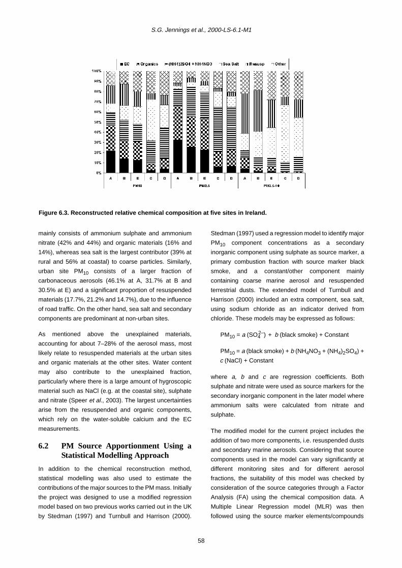
S.G. Jennings et al., 2000-LS-6.1-M1
mainly consists of ammonium sulphate and ammonium
nitrate (42% and 44%) and organic materials (16% and
14%), whereas sea salt is the largest contributor (39% at
rural and 56% at coastal) to coarse particles. Similarly,
urban site PM10 consists of a larger fraction of
carbonaceous aerosols (46.1% at A, 31.7% at B and
30.5% at E) and a significant proportion of resuspended
materials (17.7%, 21.2% and 14.7%), due to the influence
of road traffic. On the other hand, sea salt and secondary
components are predominant at non-urban sites.
As mentioned above the unexplained materials,
accounting for about 7–28% of the aerosol mass, most
likely relate to resuspended materials at the urban sites
and organic materials at the other sites. Water content
may also contribute to the unexplained fraction,
particularly where there is a large amount of hygroscopic
material such as NaCl (e.g. at the coastal site), sulphate
and nitrate (Speer et al., 2003). The largest uncertainties
arise from the resuspended and organic components,
which rely on the water-soluble calcium and the EC
measurements.
6.2 PM Source Apportionment Using aStatistical Modelling Approach
In addition to the chemical reconstruction method,
statistical modelling was also used to estimate the
contributions of the major sources to the PM mass. Initially
the project was designed to use a modified regression
model based on two previous works carried out in the UK
by Stedman (1997) and Turnbull and Harrison (2000).
Stedman (1997) used a regression model to identify major
PM10 component concentrations as a secondary
inorganic component using sulphate as source marker, a
primary combustion fraction with source marker black
smoke, and a constant/other component mainly
containing coarse marine aerosol and resuspended
terrestrial dusts. The extended model of Turnbull and
Harrison (2000) included an extra component, sea salt,
using sodium chloride as an indicator derived from
chloride. These models may be expressed as follows:
PM10 = a (SO42–) + b (black smoke) + Constant
PM10 = a (black smoke) + b (NH4NO3 + (NH4)2SO4) +
c (NaCl) + Constant
where a, b and c are regression coefficients. Both
sulphate and nitrate were used as source markers for the
secondary inorganic component in the later model where
ammonium salts were calculated from nitrate and
sulphate.
The modified model for the current project includes the
addition of two more components, i.e. resuspended dusts
and secondary marine aerosols. Considering that source
components used in the model can vary significantly at
different monitoring sites and for different aerosol
fractions, the suitability of this model was checked by
consideration of the source categories through a Factor
Analysis (FA) using the chemical composition data. A
Multiple Linear Regression model (MLR) was then
followed using the source marker elements/compounds
Figure 6.3. Reconstructed relative chemical composition at five sites in Ireland.
58

Nature and origin of PM10 and smaller particulate matter in urban air
as independent and the total particle mass concentrations
as dependent variables to calculate each source
contribution to the PM mass. The software used was
SPSS for Windows version 12.0. This procedure was
applied separately to all sites for all particle fractions as
PM10, PM2.5 and PM2.5–10. As expected, different relative
contributions from each source type and different source
strengths have been observed.
6.2.1 Factor analysis
The chemical composition data used for factor analysis
include the ionic species chloride, nitrate, sulphate, MSA,
sodium, ammonium, potassium, magnesium and calcium,
plus EC. In order to determine the secondary sulphate
(nss SO42–), sodium was used to correct for sea-salt
sulphate based on a sea salt composition with an SO42–/
Na+ ratio of 0.25. Similarly, non-sea-salt calcium (nss
Ca2+), potassium (nss K+) and magnesium (nss Mg2+)
were obtained using a sea-salt Ca2+/Na+ ratio of 0.038,
K+/Na+ ratio of 0.037 and Mg2+/Na+ ratio of 0.12.
Concentrations below the detection limit were replaced
with zero. The number of replacements was less than 5–
10% for all data sets, which has no discernible effect on
the FA results (Morandi et al., 1987).
At the first attempt, it was found that EC tended to
interfere with secondary nss SO42–, particularly at the
urban sites, presumably due to a similar source from long-
range transportation. To minimise the interference, the
EC concentrations were corrected for urban sites using
Site D as a reference site when there is a westerly air
mass, and Site C when there is an easterly air mass,
assuming that all nss SO42– and EC at Sites D and C are
attributed to long-range transportation. Therefore, EC
concentrations at urban sites were recalculated by
excluding a long-range transported component, using the
ratios nss SO42–/EC at Site D or C. Similarly,
interferences were also noticeable between EC and nss
Ca2+ at urban sites since both components are related to
road transport. However, no remedy has been applied in
this case, which may influence the outcome of the MLR
analysis.
Although statistical modelling is a traditional method and
has been used in the study of aerosol source
apportionment since the early 1970s, the procedure is not
simple and straightforward. Prior to the analysis, all data
sets were explored graphically to screen out any extreme
outliers and to check their normality since skewed
distributions and outliers can affect the results. It was
found that most of the data sets possessed a log-normal
distribution and ideally symmetrising or log-normal
transformations seem to be appropriate. This procedure
was not carried out in this study due to resultant difficulties
of subsequent interpretation. However, outliers were
screened out to make the data fit more closely to a normal
distribution, and exclusion of data points was less than
5%.
A principal component factor extraction method was used
with orthogonal (Varimax) rotation transformation. Four or
five factors (source components) were extracted with
eigenvalues over 1, which accounted for 75.8–89.2% of
the total variance. Table 6.2 shows the factors identified
with associated high loading variables (>0.7 or 0.5–0.7)
and the sum of variance explained at all sites for all
particle fractions.
The primary combustion source component is always
associated with high loadings of EC at all sites and for all
fractions, although on a few occasions high loadings of
potassium, non-sea-salt sulphate and non-sea-salt
calcium were observed. Fine potassium, which would
arise from sources such as peat burning or fireworks, can
contribute to fine aerosol mass, whereas coarse
potassium was associated with sea salt or resuspended
dusts indicated by high loadings with sea salt or
resuspended dust source components. High loadings of
nss Ca2+ at urban sites were presumably due to the fact
that both EC and nss Ca2+ are associated with road traffic,
and of nss SO42– and NO3
– at the coastal site were due
to a similar source, i.e. long-range transport.
Major loadings for the secondary inorganic source
component are shown by nitrate, sulphate and
ammonium, except at the rural site where EC also has a
contribution presumably since the EC concentrations at
Sites C and D were not corrected for excluding a fraction
associated with long-range transport.
The sea salt component has high loadings of chloride,
sodium, magnesium and sometimes potassium.
Interestingly, at Site C, nss Ca2+ and nss SO42– are also
associated with sea salt for the coarse fraction.
Resuspended dusts were characterised by high loadings
of nss Ca2+ and occasionally potassium and nss SO42– at
Sites A, B, E and D but not at Site C. High loadings of nss
SO42+ may indicate the presence of calcium sulphate in
dust materials.
59

S.G. Jennings et al., 2000-LS-6.1-M1
Significant loadings of MSA were only found at the coastal
site for the secondary marine component, which is not
included in the MLR analysis later due to low and often
zero concentrations in autumn and winter seasons.
6.2.2 MLR analysis
All five source components identified from the FA
procedure were used in the MLR analysis, which utilised
a stepwise regression method with the default variable
selection criteria Penter ≥0.050 and Premove ≤0.100.
Similarly, outliers were checked and removed following a
careful screening of the data sets before and after running
the regression model by looking at individual paired
scatter plots and plots of residuals and diagnostics.
Clearly, as Table 6.2 shows, it is reasonable to use EC,
nss Ca2+ and MSA as source indicators for primary
combustion, resuspended dusts and secondary marine
materials respectively, although MSA is not included in
the final model since its contributions to the aerosol mass
were insignificant at most of the sites except at Site C. For
testing purposes, ammonium nitrate and/or ammonium
sulphate derived from nitrate and sulphate were used as
source markers for the secondary inorganic component.
The regression models involving sulphate as a marker
often result in a negative intercept at urban sites,
presumably due to interference between long-range
transported fractions of EC and sulphate, therefore
ammonium nitrate was chosen for use in the final model
at urban sites. At the non-urban sites both nitrate and
sulphate were used, but only for the PM10 and PM2.5
fractions. Ammonium was not suitable as a tracer due to
its low concentrations, often below the detection limit, in
winter and for the coarse fractions. In the case of sea salt,
both chloride and sodium concentrations were well above
the detection limit of the chemical measurement, but
sodium was used for calculating the amount of sea salt
(NaCl) as chloride is liable to a depletion problem as
indicated earlier. Magnesium and potassium are not
considered as appropriate source markers for sea salt.
The overall finalised regression model is expressed as:
PM = a (EC) + b (NH4NO3) + c (NaCl) + d (nss Ca) +
Constant
where a, b, c and d are regression coefficients, and the
constant indicates unexplained/other components.
Table 6.2. Resul ts of factor analys is (source componen ts and assoc iated var iables w ith strong load ing – >0.7 or*0.5–0.7).Sites Fraction Primary
combustionSecondarycombustion
Sea salt Resuspended dusts Secondarymarine
Sum of variance
(%)
A PM10 EC NO3–, nss SO4
2–, NH4+ Cl–, Na+, Mg2+ nss Ca2+, K+ N/A 85.9
PM2.5 EC NO3–, nss SO4
2–, NH4+ Cl–, Na+, Mg2+ nss Ca2+ MSA 88.5
PM2.5–10 EC, *nss Ca2+ NO3–, NH4
+ Cl–, Na+, Mg2+ nss Ca2+, K+ N/A 83.0
B PM10 EC, K+ NO3–, nss SO4
2–, NH4+ Cl–, Na+, Mg2+ nss Ca2+ N/A 81.5
PM2.5 EC, K+ NO3–, nss SO4
2–, NH4+ Cl–, Na+, Mg2+ nss Ca2+ N/A 86.2
PM2.5–10 EC NO3–, *nss SO4
2–, NH4+ Cl–, Na+, Mg2+, K+ nss Ca2+ N/A 85.6
E PM10 EC NO3–, nss SO4
2–, NH4+ Cl–, Na+, Mg2+, *K+ nss Ca2+, *K+ N/A 81.5
PM2.5 EC NO3–, nss SO4
2–, NH4+ Cl–, Na+, Mg2+ nss Ca2+, *K+ N/A 80.0
PM2.5–10 EC, *nss Ca2+ NO3–, *nss SO4
2–, NH4+ Cl–, Na+, Mg2+, K+ nss Ca2+, *nss SO4
2– N/A 75.8
C PM10 EC, *nss SO42– NO3
–, nss SO42–, NH4
+ Cl–, Na+, Mg2+, K+ N/A MSA 84.7
PM2.5 EC, *NO3– nss SO4
2–, NH4+ Cl–, Na+, Mg2+ N/A MSA 80.3
PM2.5–10 EC NO3–, NH4
+ Cl–, Na+, Mg2+, K+, *nss Ca2+, *nss SO4
2–N/A MSA 89.2
D PM10 EC NO3–, nss SO4
2–, NH4+,
*ECCl–, Na+, Mg2+ nss Ca2+, K+ N/A 86.9
PM2.5 EC NO3–, nss SO4
2–, NH4+,
*ECCl–, Na+, Mg2+ nss Ca2+ N/A 88.5
PM2.5–10 EC NO3–, NH4
+ Cl–, Na+, Mg2+ nss Ca2+, nss SO42– ,
K+N/A 81.9
60

Nature and origin of PM10 and smaller particulate matter in urban air
6.2.2.1 Results of MLR
Table 6.3 shows the model results, regression
coefficients, coupled with standardised coefficients β, and
the adjusted R2. The significance values of the t-statistics
for all regression coefficients are less than 0.05, except at
the coastal site, for nss Ca2+, the coefficients are not
significant and were excluded from the model.
Reasonable model fits were obtained using the above
four predictor variables and a constant variable, giving an
average coefficient of determination of R2 = 0.87 (range:
0.77–0.98), indicating that 77–98% of the total variance in
the total aerosol mass was accounted for by the model.
The EC coefficient a is much larger than unity as this
marker element represents primary combustion materials
covering not only EC but also organic and other related
materials. Interestingly, those coefficients were smaller at
urban sites (smallest at Site A) than at non-urban sites,
indicative of a higher proportion of EC in the
carbonaceous particles at urban sites due to a high
vehicle exhaust contribution. Furthermore, the
coefficients for fine fractions were smaller than for coarse
fractions, again reflecting the importance of EC
contributing to fine particles.
Similarly, values of coefficient b were greater (2.38–3.49)
when only ammonium nitrate was used as a secondary
source marker at the urban sites, but close to unity (1.14–
1.24) when a combined ammonium nitrate and
ammonium sulphate source marker was used at non-
urban sites. The PM10 coefficient of 1.24 at Site C is
higher than that (0.83) determined for the Lizard coastal
site in the UK, while 1.14 at Site D is close to those
obtained (1.01 and 1.36) for the rural Lichfield and
Pershore sites in the UK (Turnbull and Harrison, 2000). In
the case of coarse particles, the coefficients were lower in
comparison with fine particles since ammonium sulphate
can compose a large part of the secondary materials
mainly in the fine particle mode.
Sea-salt coefficients c were generally consistent at all
sites and for all fractions and more or less close to unity
indicating that this component is mostly composed of
sodium chloride and is a significant contributor to aerosol
mass in the Ireland atmosphere, which is clearly seen
from the estimated sea salt PM10 concentrations of 2.9–
4.7 µg/m3 (Table 6.4).
Non-sea-salt calcium was used as a source indicator for
resuspended dusts, a source component not included in
the previous models of Stedman et al. (2001) and Turnbull
Table 6.3. Results of multi-linear regression.Fractions Sites Regression coefficients and beta coefficients (β) Constant R2
ECa (β)
NH4NO3
b (β)NaClc (β)
nss Cad (β)
PM10 A 2.18 (0.36) 2.38 (0.48) 1.05 (0.15) 6.63 (0.43) 2.34 0.88
B 2.76 (0.40) 2.47 (0.56) 0.89 (0.24) 4.10 (0.20) 2.49 0.84
E 2.88 (0.37) 2.68 (0.60) 1.12 (0.36) 6.04 (0.26) 2.40 0.84
C 4.25 (0.15) *1.24 (0.56) 1.25 (0.88) – 1.96 0.95
D 4.21 (0.33) *1.14 (0.68) 1.21 (0.41) 4.01 (0.09) 1.36 0.94
PM2.5 A 2.23 (0.16) 2.89 (0.64) 0.84 (0.07) 5.14 (0.06) 2.16 0.78
B 2.35 (0.46) 2.87 (0.60) 0.81 (0.08) 1.44 (0.02) 1.92 0.77
E 2.81 (0.48) 3.49 (0.63) 1.01 (0.08) 2.87 (0.05) 1.21 0.77
C 3.11 (0.23) *1.14 (0.82) 1.20 (0.33) – 0.44 0.97
D 3.98 (0.38) *1.19 (0.69) 1.10 (0.15) 4.03 (0.04) 0.50 0.96
PM2.5–10 A 3.70 (0.28) 1.52 (0.23) 1.21 (0.38) 5.51 (0.60) 1.52 0.91
B 8.46 (0.20) 1.23 (0.25) 1.07 (0.48) 4.14 (0.49) 1.51 0.89
E 6.24 (0.21) 1.54 (0.20) 1.15 (0.56) 5.57 (0.54) 1.48 0.83
C 9.90 (0.02) 1.61 (0.18) 1.21 (0.98) – 1.68 0.98
D 11.77 (0.07) 1.21 (0.28) 1.26 (0.73) 4.21 (0.23) 0.72 0.81
*NH4NO3 + (NH4)2SO4 was used as an indicator for the secondary inorganic source.
61
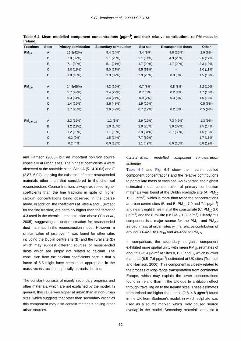
S.G. Jennings et al., 2000-LS-6.1-M1
and Harrison (2000), but an important pollution source
especially at urban sites. The highest coefficients d were
observed at the roadside sites, Sites A (5.14–6.63) and E
(2.87–6.04), implying the existence of other resuspended
materials other than that considered in the chemical
reconstruction. Coarse fractions always exhibited higher
coefficients than the fine fractions in spite of higher
calcium concentrations being observed in the coarse
mode. In addition, the coefficients at Sites A and E (except
for the fine fraction) are certainly higher than the factor of
4.3 used in the chemical reconstruction above (Yin et al.,
2005), suggesting an underestimation for resuspended
dust materials in the reconstruction model. However, a
similar value of just over 4 was found for other sites
including the Dublin centre site (B) and the rural site (D)
which may suggest different sources of resuspended
dusts which are simply not related to calcium. The
conclusion from the calcium coefficients here is that a
factor of 5.5 might have been most appropriate in the
mass reconstruction, especially at roadside sites.
The constant consists of mainly secondary organics and
other materials, which are not explained by the model. In
general, this value was higher at urban than at non-urban
sites, which suggests that other than secondary organics
this component may also contain materials having other
urban sources.
6.2.2.2 Mean modelled component concentration
estimates
Table 6.4 and Fig. 6.4 show the mean modelled
component concentrations and the relative contributions
to particulate mass at each site. As expected, the highest
estimated mean concentration of primary combustion
materials was found at the Dublin roadside site (A: PM10
15.8 µg/m3), which is more than twice the concentrations
at urban centre sites (B and E: PM10 7.0 and 7.1 µg/m3)
and nearly eight times that at the coastal site (C: PM10 2.0
µg/m3) and the rural site (D: PM10 1.8 µg/m3). Clearly this
component is a major source for the PM10 and PM2.5
aerosol mass at urban sites with a relative contribution of
around 30–42% to PM10 and 49–65% to PM2.5.
In comparison, the secondary inorganic component
exhibited more spatial unity with mean PM10 estimates of
about 5.0–5.4 µg/m3 at Sites A, B, E and C, which is lower
than that (6.5–7.6 µg/m3) estimated at UK sites (Turnbull
and Harrison, 2000). This component is closely related to
the process of long-range transportation from continental
Europe, which may explain the lower concentrations
found in Ireland than in the UK due to a dilution effect
through travelling on to the Ireland sites. These estimates
from Ireland are higher than those (2.8–4.8 µg/m3) found
in the UK from Stedman’s model, in which sulphate was
used as a source marker, which likely caused source
overlap in the model. Secondary materials are also a
Table 6.4. Mean modelled component concentrations ( µg/m3) and their relative contributions to PM mass inIreland.Fractions Sites Primary combustion Secondary combustion Sea salt Resuspended dusts Other
PM10 A 15.8(42%) 5.4 (14%) 3.4 (9%) 9.8 (26%) 2.9 (8%)
B 7.0 (32%) 5.1 (23%) 3.1 (14%) 4.3 (20%) 2.6 (12%)
E 7.1 (30%) 5.1 (21%) 4.7 (20%) 4.7 (20%) 2.3 (10%)
C 2.0 (11%) 5.0 (27%) 9.5 (51%) – 2.0 (11%)
D 1.8 (18%) 3.3 (32%) 2.9 (28%) 0.8 (8%) 1.5 (15%)
PM2.5 A 14.5(65%) 4.2 (19%) 0.7 (3%) 0.8 (3%) 2.2 (10%)
B 5.7 (49%) 3.4 (29%) 0.7 (6%) 0.2 (1%) 1.7 (15%)
E 6.3 (51%) 3.4 (27%) 0.9 (7%) 0.3 (3%) 1.6 (13%)
C 1.4 (19%) 3.6 (48%) 1.9 (26%) – 0.5 (6%)
D 1.7 (28%) 2.9 (49%) 0.7 (12%) 0.2 (3%) 0.5 (9%)
PM2.5–10 A 2.2 (15%) 1.2 (8%) 2.9 (19%) 7.3 (49%) 1.3 (9%)
B 1.2 (11%) 1.0 (10%) 2.9 (28%) 3.9 (37%) 1.5 (14%)
E 1.2 (10%) 1.1 (10%) 3.9 (34%) 3.7 (33%) 1.5 (13%)
C 0.2 (2%) 1.5 (14%) 7.7 (69%) – 1.7 (15%)
D 0.2 (4%) 0.6 (13%) 2.1 (49%) 0.6 (15%) 0.8 (19%)
62
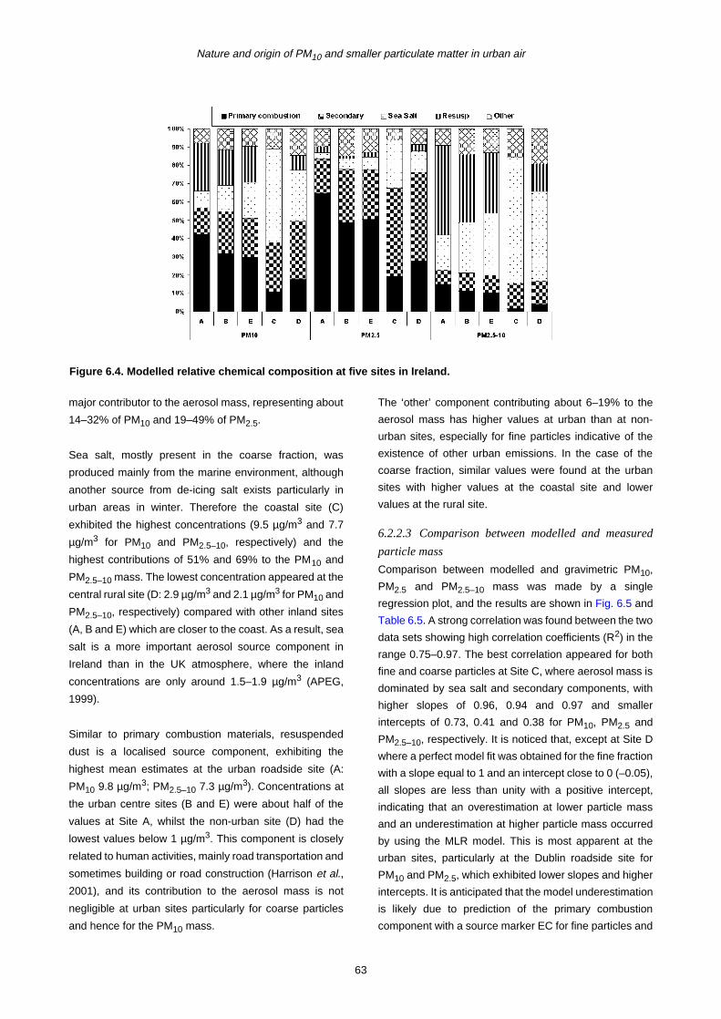
Nature and origin of PM10 and smaller particulate matter in urban air
major contributor to the aerosol mass, representing about
14–32% of PM10 and 19–49% of PM2.5.
Sea salt, mostly present in the coarse fraction, was
produced mainly from the marine environment, although
another source from de-icing salt exists particularly in
urban areas in winter. Therefore the coastal site (C)
exhibited the highest concentrations (9.5 µg/m3 and 7.7
µg/m3 for PM10 and PM2.5–10, respectively) and the
highest contributions of 51% and 69% to the PM10 and
PM2.5–10 mass. The lowest concentration appeared at the
central rural site (D: 2.9 µg/m3 and 2.1 µg/m3 for PM10 and
PM2.5–10, respectively) compared with other inland sites
(A, B and E) which are closer to the coast. As a result, sea
salt is a more important aerosol source component in
Ireland than in the UK atmosphere, where the inland
concentrations are only around 1.5–1.9 µg/m3 (APEG,
1999).
Similar to primary combustion materials, resuspended
dust is a localised source component, exhibiting the
highest mean estimates at the urban roadside site (A:
PM10 9.8 µg/m3; PM2.5–10 7.3 µg/m3). Concentrations at
the urban centre sites (B and E) were about half of the
values at Site A, whilst the non-urban site (D) had the
lowest values below 1 µg/m3. This component is closely
related to human activities, mainly road transportation and
sometimes building or road construction (Harrison et al.,
2001), and its contribution to the aerosol mass is not
negligible at urban sites particularly for coarse particles
and hence for the PM10 mass.
The ‘other’ component contributing about 6–19% to the
aerosol mass has higher values at urban than at non-
urban sites, especially for fine particles indicative of the
existence of other urban emissions. In the case of the
coarse fraction, similar values were found at the urban
sites with higher values at the coastal site and lower
values at the rural site.
6.2.2.3 Comparison between modelled and measured
particle mass
Comparison between modelled and gravimetric PM10,
PM2.5 and PM2.5–10 mass was made by a single
regression plot, and the results are shown in Fig. 6.5 and
Table 6.5. A strong correlation was found between the two
data sets showing high correlation coefficients (R2) in the
range 0.75–0.97. The best correlation appeared for both
fine and coarse particles at Site C, where aerosol mass is
dominated by sea salt and secondary components, with
higher slopes of 0.96, 0.94 and 0.97 and smaller
intercepts of 0.73, 0.41 and 0.38 for PM10, PM2.5 and
PM2.5–10, respectively. It is noticed that, except at Site D
where a perfect model fit was obtained for the fine fraction
with a slope equal to 1 and an intercept close to 0 (–0.05),
all slopes are less than unity with a positive intercept,
indicating that an overestimation at lower particle mass
and an underestimation at higher particle mass occurred
by using the MLR model. This is most apparent at the
urban sites, particularly at the Dublin roadside site for
PM10 and PM2.5, which exhibited lower slopes and higher
intercepts. It is anticipated that the model underestimation
is likely due to prediction of the primary combustion
component with a source marker EC for fine particles and
Figure 6.4. Modelled relative chemical composition at five sites in Ireland.
63
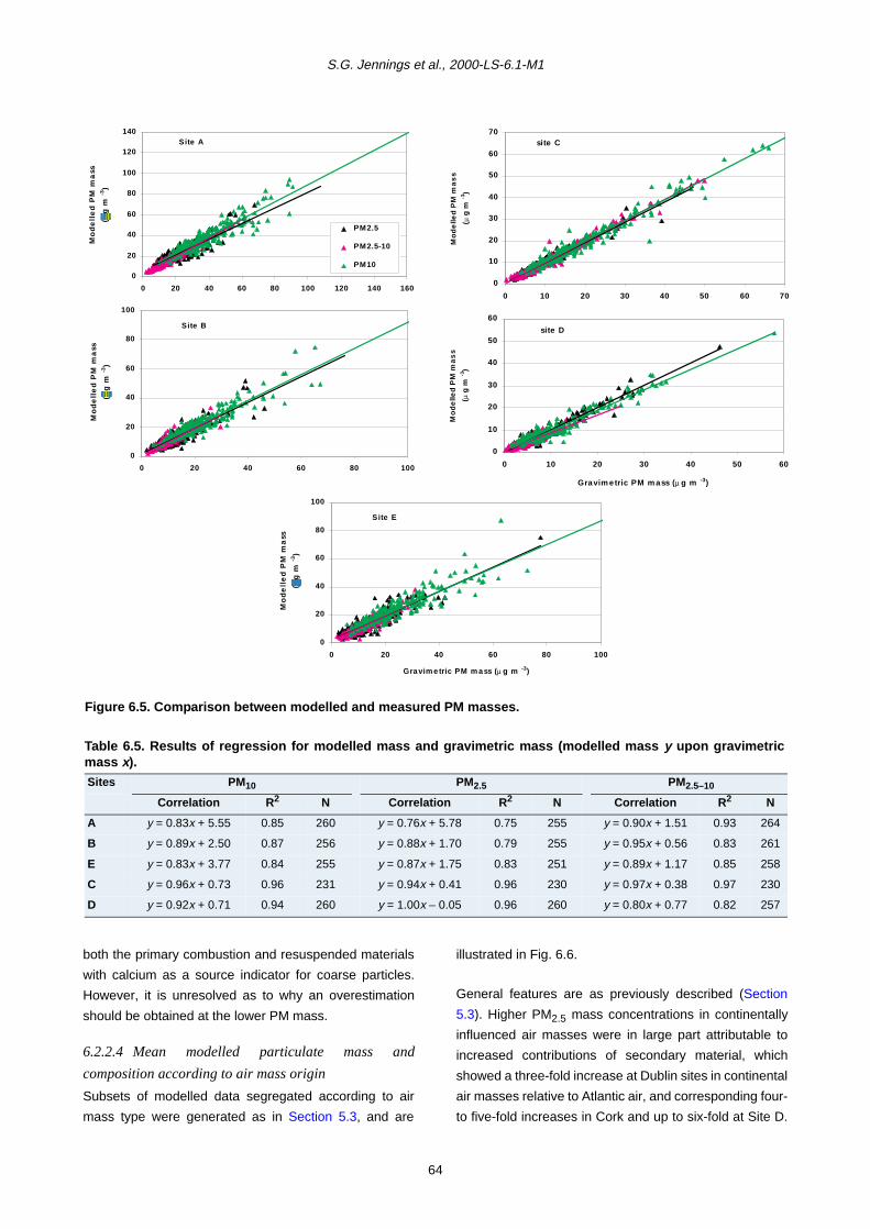
S.G. Jennings et al., 2000-LS-6.1-M1
both the primary combustion and resuspended materials
with calcium as a source indicator for coarse particles.
However, it is unresolved as to why an overestimation
should be obtained at the lower PM mass.
6.2.2.4 Mean modelled particulate mass and
composition according to air mass origin
Subsets of modelled data segregated according to air
mass type were generated as in Section 5.3, and are
illustrated in Fig. 6.6.
General features are as previously described (Section
5.3). Higher PM2.5 mass concentrations in continentally
influenced air masses were in large part attributable to
increased contributions of secondary material, which
showed a three-fold increase at Dublin sites in continental
air masses relative to Atlantic air, and corresponding four-
to five-fold increases in Cork and up to six-fold at Site D.
Figure 6.5. Comparison between modelled and measured PM masses.
Table 6.5. Results of regression for modelled mass and gravimetric mass (modelled mass y upon gravimetricmass x).Sites PM10 PM2.5 PM2.5–10
Correlation R2 N Correlation R2 N Correlation R2 N
A y = 0.83x + 5.55 0.85 260 y = 0.76x + 5.78 0.75 255 y = 0.90x + 1.51 0.93 264
B y = 0.89x + 2.50 0.87 256 y = 0.88x + 1.70 0.79 255 y = 0.95x + 0.56 0.83 261
E y = 0.83x + 3.77 0.84 255 y = 0.87x + 1.75 0.83 251 y = 0.89x + 1.17 0.85 258
C y = 0.96x + 0.73 0.96 231 y = 0.94x + 0.41 0.96 230 y = 0.97x + 0.38 0.97 230
D y = 0.92x + 0.71 0.94 260 y = 1.00x – 0.05 0.96 260 y = 0.80x + 0.77 0.82 257
Site E
0
20
40
60
80
100
0 20 40 60 80 100
Gravime tric PM mass (µ g m -3)
Mo
de
lle
d P
M m
ass
(g
m -3
)
site C
0
10
20
30
40
50
60
70
0 10 20 30 40 50 60 70
Mo
de
lled
PM
ma
ss
(µg
m -3
)
site D
0
10
20
30
40
50
60
0 10 20 30 40 50 60
Gravim etric PM m ass (µ g m -3)
Mo
de
lled
PM
ma
ss
(µg
m -3
)
S ite A
0
20
40
60
80
100
120
140
0 20 40 60 80 100 120 140 160
Mo
de
lle
d P
M m
ass
(g
m -3
)
PM2.5
PM2.5-10
PM10
Site B
0
20
40
60
80
100
0 20 40 60 80 100
Mo
de
lle
d P
M m
ass
(g
m -3
)
64
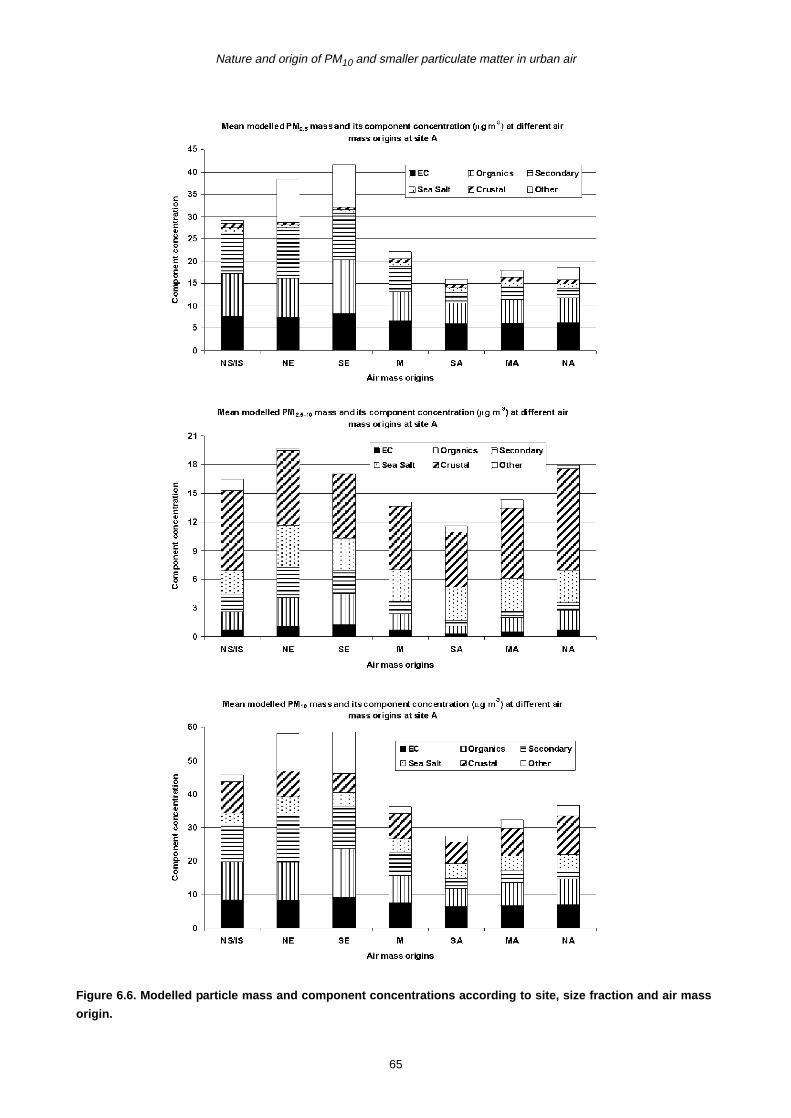
Nature and origin of PM10 and smaller particulate matter in urban air
Figure 6.6. Modelled particle mass and component concentrations according to site, size fraction and air mass
origin.
65

S.G. Jennings et al., 2000-LS-6.1-M1
Figure 6.6. Contd.
66

Nature and origin of PM10 and smaller particulate matter in urban air
Figure 6.6. Contd.
67

S.G. Jennings et al., 2000-LS-6.1-M1
Figure 6.6. Contd.
68

Nature and origin of PM10 and smaller particulate matter in urban air
Figure 6.6. Contd.
69

S.G. Jennings et al., 2000-LS-6.1-M1
The OC fraction was also present at higher levels in
continental air masses; in the absence of local sources
(Site D is the best example) these air masses contained
three to five times as much fine fraction organic material
as the Atlantic air masses. At the Dublin urban sites, OC
levels in continental air masses were around twice those
in Atlantic air, while the difference was somewhat lower in
Cork. There is evidence for higher levels of fine (and
coarse) mode crustal (resuspended) material during
continental type events at Sites C, D and E, but not at the
Dublin sites, where differences were probably obscured
by the predominance of locally generated dusts. Fine
fraction sea salt levels were similar in all air mass types at
all sites, with sea salt only contributing a minor fraction of
PM2.5 at urban locations. However, sea salt was a
significant component of PM10, showing no sector
association in Dublin but higher levels in Atlantic air in
Cork.
6.3 Comparison between Modelled andReconstructed Component Mass
Comparison was also made between the modelled (Table
6.4) and reconstructed (Table 6.6) component mass. In
general, fine mode modelled concentrations of primary
combustion components are slightly lower than the sum of
reconstructed concentrations for EC and organics, in
which secondary organic compounds were included. For
coarse fractions, however, except for Site A, the modelled
concentrations were higher than reconstructed. As a
result, for PM10, urban sites exhibited similar or slightly
lower modelled values for primary combustion materials
in comparison with the reconstructed results, but non-
urban sites showed much higher modelled concentrations
of this component, indicating an underestimation for
organic compounds in the reconstructed mass. Similar or
slightly higher secondary and sea salt component
concentrations were modelled compared with those
reconstructed. At the coastal site, a much larger value of
coarse sea salt (7.7 µg/m3) was modelled and hence a
higher concentration of PM10 (9.5 µg/m3), whereas the
reconstructed values were 6.3 µg/m3 and 7.4 µg/m3 for
the coarse mode and PM10, respectively. Most
interestingly, the Dublin roadside site gave a much
greater PM10 value for resuspended dusts from modelled
results (9.8 µg/m3) than from reconstructed results (6.5
µg/m3), indicative of an underestimation in the chemical
reconstruction using 4.3 × Ca2+. A similar finding occurred
at Site E but not at Site B.
In general terms, the PM mass was better explained by
the MLR model (81–92%) than by the chemical
reconstruction (72–93%) using similar source markers.
The major advantage of the regression model is seen
Table 6.6. Mean reconstructed component concentrations ( µg/m3) and their contributions to PM mass (%) inIreland.
Fractions Sites EC Organics Secondary Sea salt Resuspended dusts Other
PM10 A 7.9 (22%) 9.0 (25%) 4.8 (13%) 3.2 (9%) 6.5 (18%) 6.1 (14%)
B 3.1 (14%) 3.9 (17%) 4.5 (20%) 3.2 (14%) 4.7 (21%) 2.8 (12%)
E 3.0 (13%) 4.3 (18%) 4.1 (17%) 4.2 (18%) 3.5 (15%) 4.8 (20%)
C 0.5 (3%) 1.1 (6%) 4.3 (23%) 7.4 (40%) 1.2 (6%) 4.0 (22%)
D 0.4 (4%) 1.0 (10%) 3.2 (30%) 2.3 (22%) 1.0 (10%) 2.4 (24%)
PM2.5 A 7.3 (33%) 7.4 (33%) 3.8 (17%) 0.7 (3%) 0.6 (3%) 2.6 (12%)
B 3.0 (26%) 3.5 (29%) 3.4 (29%) 0.6 (5%) 0.5 (4%) 0.8 (7%)
E 2.9 (23%) 3.8 (30%) 3.3 (26%) 0.8 (7%) 0.5 (4%) 1.2 (10%)
C 0.5 (6%) 1.1 (14%) 3.3 (44%) 1.1 (15%) 0.3 (4%) 1.2 (16%)
D 0.4 (7%) 1.0 (16%) 2.5 (42%) 0.6 (11%) 0.2 (3%) 1.3 (21%)
PM2.5–10 A 0.6 (4%) 1.6 (11%) 1.1 (7%) 2.5 (17%) 5.9 (39%) 3.3 (22%)
B 0.1 (1%) 0.4 (4%) 1.1 (10%) 2.6 (25%) 4.2 (41%) 1.9 (19%)
E 0.2 (2%) 0.6 (5%) 0.9 (8%) 3.4 (30%) 3.1 (27%) 3.2 (28%)
C 0.02(0.2%) 0.1 (1%) 1.1 (9%) 6.3 (56%) 0.9 (8%) 2.8 (25%)
D 0.01(0.3%) 0.05 (1%) 0.6 (14%) 1.7 (39%) 0.8 (18%) 1.2 (28%)
70

Nature and origin of PM10 and smaller particulate matter in urban air
from the calculation of resuspended dusts, in which
different factors were assigned for each site and for
different fractions due to a varied dust composition, whilst
a fixed factor was used in the chemical reconstruction.
Errors in regression models may arise from careless
selection of source indicators, skewed distributions,
outliers and source overlaps; however such errors have
been minimised here. The simplicity of the chemical
reconstruction procedure may be more advantageous
when source markers and source composition are clear,
such as for secondary inorganic and sea salt
components.
6.4 Results of the Revised ChemicalReconstruction
It is important to notice that the MLR method accounts for
the water associated with the hygroscopic components
through the coefficients as seen in Table 6.3, which is
probably why MLR analysis accounts for a larger
proportion of the mass. Similarly with the resuspended
component, a better estimation is achieved with the MLR
model. Therefore an improvement of the chemical
reconstruction can be made based on the statistical
model results in Table 6.3.
In order to allow for bound water (or other matter not
measured) for hygroscopic particles such as sodium
chloride and ammonium salts, the water (or other
material) contents were estimated and added to the sea
salt, sulphate and nitrate. For sodium chloride at Site C,
the coefficient is 1.25, suggesting that a further 25% of the
value should be added to the NaCl mass in the mass
reconstruction method. Similarly, for the sum of
ammonium nitrate and ammonium sulphate at Sites C and
D, the coefficients suggest that about 20–25%,
representing bound water (or other material), should be
added. As a result, a further 25% of the mass was added
to these components. The results for calcium in the
coarse particle fraction suggest that a factor of 5.5 might
have been most appropriate in the mass reconstruction.
In other words, about 22% should have been added to the
mass of the resuspended dust to include materials other
than gypsum, but associated with this source.
Table 6.7 and Fig. 6.7 show the corrected reconstructed
chemical component concentrations and the relative
chemical composition. The ‘other’ component
concentrations were significantly reduced by about 48–
100% after the adjustment for additional material (mainly
hygroscopic and resuspended materials). A much better
mass closure is seen in Fig. 6.6 with the relative
contributions of the ‘other’ component to the aerosol mass
dropping from above 10% (7–28%) to below 10% (1–
13%).
The annual (2002) average relative chemical composition
is shown in Table 6.8 for the three PM categories at all
Table 6.7. Mean corrected reconstructed PM component and to tal concentrations ( µg/m3) in Ireland.Fractions Sites Total EC Organics Secondary Sea salt Resuspended dusts Other
PM10 A 37.3 7.9 9.0 6.0 4.0 7.9 2.7
B 22.1 3.1 3.9 5.6 4.0 5.7 –0.2
E 23.9 3.0 4.3 5.1 5.3 4.3 1.9
C 18.6 0.5 1.1 5.4 9.3 1.4 0.8
D 10.4 0.4 1.0 3.9 2.9 1.2 0.9
PM2.5 A 22.4 7.3 7.4 4.7 0.9 0.8 1.4
B 11.7 3.0 3.5 4.3 0.7 0.6 –0.3
E 12.5 2.9 3.8 4.1 1.1 0.6 0.1
C 7.4 0.5 1.1 4.1 1.4 0.3 0.1
D 6.0 0.4 1.0 3.2 0.8 0.3 0.4
PM2.5–10 A 14.9 0.6 1.6 1.3 3.1 7.2 1.1
B 10.4 0.1 0.4 1.3 3.2 5.1 0.1
E 11.4 0.2 0.6 1.1 4.2 3.8 1.4
C 11.2 0.0 0.1 1.3 7.8 1.1 0.8
D 4.3 0.0 0.0 0.8 2.1 0.9 0.5
71

S.G. Jennings et al., 2000-LS-6.1-M1
sites in terms of the following chemical composition
categories: sea salt, primary (EC), organics, secondary
organics, crustal (or resuspended matter) and ‘other’ as
explained in more detail in Section 6.1.2. Seasonally
averaged relative chemical data are shown in Table 6.9.
The remaining ‘other’ component concentrations are
highest at Sites A and E for the PM2.5–10 fraction, and
probably contain both resuspended and organic
materials. These resuspended materials must not be
covered by the 22% increment as they are not related to
calcium and not reflected in the calcium coefficient. In the
case of Sites C and D, the ‘other’ component is mainly
related to organic material, which is clearly
underestimated using the very low EC concentrations for
the coarse mode. Similarly, considering the PM2.5 and
PM10, underestimation may occur for the organic
component at non-urban sites and for both organic and
resuspended components at urban sites. At Site B only,
Table 6.8. Annual (2002) average relative chemical composition.Site(%)
Sea Salt(%)
Primary (EC)(%)
Organics(%)
Secondary inorganic(%)
Crustal(%)
Other(%)
PM10 A 13.0 24.5 23.6 15.3 18.7 5.0
B 20.5 14.1 16.6 24.8 23.9 0.2
E 24.6 12.5 17.4 20.3 18.6 6.7
C 44.6 2.7 9.6 31.7 7.3 4.1
D 31.3 3.9 12.9 34.1 11.9 5.8
PM2.5 A 4.8 39.2 33.8 19.4 3.2 –0.4
B 7.5 27.1 30.1 36.2 5.4 –6.2
E 10.6 23.3 29.8 30.3 4.4 1.6
C 21.7 5.9 20.6 53.8 3.5 –5.5
D 15.5 6.9 22.9 48.8 6.0 –0.2
PM2.5–10 A 23.4 3.2 8.5 10.1 41.2 13.5
B 31.9 1.0 3.1 13.6 43.6 6.7
E 38.5 1.6 5.0 9.9 33.7 11.4
C 59.9 0.2 0.7 16.0 11.1 12.1
D 47.6 0.4 1.3 18.9 22.0 9.8
Figure 6.7. Corrected reconstructed relative chemical composition at five sites in Ireland.
72

Nature and origin of PM10 and smaller particulate matter in urban air
Table 6.9. Seasonal average relative chemical composition.Sea salt
(%)Primary (EC)
(%)Organics
(%)Secondary inorganic
(%)Crustal
(%)Other
(%)Site A PM10 Spring 14.6 21.5 20.0 17.3 19.3 7.3
Summer 7.4 27.7 27.7 13.2 19.8 4.2
Autumn 10.6 26.2 25.9 15.5 16.9 5.1
Winter 19.4 22.6 20.8 15.0 18.9 3.3
PM2.5 Spring 4.2 34.7 28.0 22.4 2.8 7.8
Summer 2.1 43.7 39.0 16.2 3.2 –4.3
Autumn 3.4 40.1 36.0 18.5 2.6 –0.6Winter 9.3 38.3 32.2 20.4 4.2 –4.4
PM2.5–10 Spring 28.3 3.3 8.4 9.6 42.7 7.7
Summer 14.3 2.6 9.1 8.8 44.9 20.3
Autumn 19.5 4.0 10.1 13.0 39.8 13.5
Winter 31.4 3.1 6.4 9.1 37.5 12.5
Site B PM10 Spring 23.9 12.1 14.4 24.5 25.8 –0.8Summer 14.4 13.3 17.8 25.8 26.9 1.8
Autumn 16.4 17.8 19.4 25.8 21.8 –1.2
Winter 27.1 13.1 14.7 23.3 21.0 0.8
PM2.5 Spring 7.7 23.5 25.9 36.1 5.5 1.4
Summer 5.5 27.0 34.0 40.3 5.8 –12.5
Autumn 5.2 33.6 35.4 33.8 3.9 –12.0
Winter 11.6 24.3 25.1 34.5 6.3 –1.8PM2.5–10 Spring 39.7 1.0 3.0 12.3 46.9 –2.9
Summer 18.8 0.8 2.7 12.2 49.6 15.9
Autumn 28.1 0.7 2.2 17.7 41.4 9.9
Winter 41.2 1.6 4.4 12.3 36.5 4.1
Site E PM10 Spring 26.7 11.5 15.6 25.0 17.7 3.5
Summer 21.9 12.2 17.3 14.2 25.8 8.6Autumn 14.2 15.1 20.9 26.5 18.0 5.3
Winter 35.6 11.2 15.8 15.5 12.7 9.3
PM2.5 Spring 12.9 21.7 27.5 38.3 4.8 –5.2
Summer 8.2 24.5 30.9 24.5 6.9 5.1
Autumn 5.0 26.4 33.9 36.6 2.7 –4.6
Winter 16.2 20.6 26.9 21.9 3.4 11.0PM2.5–10 Spring 40.4 1.2 3.6 10.5 32.7 11.5
Summer 32.3 1.8 6.3 6.0 43.0 10.6
Autumn 32.5 1.6 5.0 12.6 33.2 15.1
Winter 48.9 1.8 5.1 10.3 25.7 8.2
Site C PM10 Spring 45.1 2.5 9.4 30.7 6.1 6.3
Summer 32.2 2.8 11.9 37.5 9.0 6.5Autumn 41.7 3.0 10.4 37.2 6.4 1.3
Winter 59.5 2.4 6.8 21.5 7.7 2.1
PM2.5 Spring 20.2 5.0 18.6 51.0 2.0 3.1
Summer 11.8 5.6 23.7 63.7 4.3 –9.2
Autumn 20.4 6.8 22.7 56.4 3.2 –9.4
Winter 34.4 6.2 17.3 44.1 4.4 –6.4
PM2.5–10 Spring 63.3 0.3 0.9 16.2 9.9 9.4Summer 48.1 0.2 0.8 15.6 13.5 21.7
Autumn 54.9 0.2 0.7 21.9 11.0 11.3
Winter 73.3 0.1 0.4 10.3 9.9 6.0
Site D PM10 Spring 33.3 3.2 11.6 32.1 9.9 9.9
Summer 33.9 2.6 10.9 32.9 14.6 5.1
Autumn 26.2 4.9 15.4 36.6 11.4 5.5Winter 31.7 5.0 13.9 34.9 11.6 2.8
PM2.5 Spring 16.8 5.6 20.0 45.6 4.2 7.9
Summer 15.3 5.0 21.1 53.6 7.5 –2.6
Autumn 13.6 8.8 27.2 48.7 5.2 –3.4
Winter 16.5 8.4 23.5 47.2 7.1 –2.8
PM2.5–10 Spring 52.3 0.3 1.2 15.7 20.6 9.7Summer 49.9 0.3 1.1 15.7 22.6 10.4
Autumn 40.9 0.3 0.8 24.7 21.9 11.3
Winter 47.1 0.7 1.9 19.5 23.1 7.8
73

S.G. Jennings et al., 2000-LS-6.1-M1
the fine and the total mass were overestimated by 3% and
1%, respectively.
Based on the improved reconstruction method, a much
higher proportion, about 87–100%, of the aerosol mass
can be accounted for, compared with the uncorrected
reconstruction and the statistical methods, which explain
about 72–93% and 81–92%, respectively. It is clear that
using the results of the MLR analysis, the chemical
reconstruction can be improved well beyond the
regression model. Furthermore, it would be possible to
obtain a 100% or close to a 100% chemical reconstruction
for all particle size fractions at all sites if we were to make
a direct measurement of the elemental and OC contents
instead of an indirect measurement and estimation, and to
use both water-soluble and insoluble calcium (the latter
was not measured as daily data) rather than only the
soluble content.
Contribution of local source components to PM total
gravimetric mass was estimated by comparing Sites A, B,
E and C with D, assuming that all particles at Site D are
long-range or regionally transported. The contribution of
local source components to PM and the total mass
contribution from local sources (sum of each component)
are shown in Table 6.10 for the three PM particle
categories over the whole measurement period of 18
months. The first column is the total contribution of local
sources to the total PM mass. For example, the
contribution of local sea salt at Site E is 7.9% to PM10
mass, and total contribution of all local sources to PM10
mass is 56.6%. Therefore the non-local sources will be
43.4%, which includes sea salt, EC, organics, secondary,
crustal and other matter.
Table 6.10. Contribution of local sources to PM.Sites(%)
Mass(%)
Sea salt(%)
Primary (EC)(%)
Organics(%)
Secondary inorganic(%)
Crustal(%)
Other(%)
PM10 A 72.3 2.4 20.2 20.9 4.8 14.8 9.2
B 53.1 3.8 12.3 11.0 6.0 16.7 3.3
E 56.6 7.9 10.8 12.0 3.9 10.6 11.5
C 44.2 27.4 0.2 1.0 6.4 0.9 8.2
PM2.5 A 73.0 0.5 31.0 27.8 6.0 1.8 5.9
B 49.7 0.0 22.1 17.8 7.6 2.2 0.0
E 51.8 1.7 19.6 19.4 5.8 2.1 3.3
C 19.8 6.5 0.5 2.4 9.9 0.5 0.0
PM2.5–10 A 71.1 5.3 4.0 10.5 3.1 34.3 13.8
B 58.3 8.8 1.3 3.6 4.3 33.2 7.0
E 62.0 14.9 1.6 4.5 2.8 20.7 17.5
C 61.3 41.2 0.0 0.1 4.1 1.2 14.7
74

Nature and origin of PM10 and smaller particulate matter in urban air
7 Metals
7.1 Sources of Trace Metals
Calcium (Ca)
Calcium is mainly crustal in origin and is associated with
rocks and soils that enter the atmosphere mainly from
resuspension of surface dusts. It is usually found in higher
concentrations in the coarse fraction (Harrison and Jones,
1995; Horvath et al., 1996; Harrison et al., 2003a).
Manganese (Mn)
Manganese can have both crustal and anthropogenic
origins (Harrison et al., 2003a). It can occur in both the
coarse and fine fractions. The coarse fraction results from
erosion of soils (Harrison and Jones, 1995), and the fine
fraction can result from higher temperature combustion of
manganese-rich fuel enhancers or smelting (Spokes et
al., 2001), but also from incineration and modern coal-
fired power plants (Horvath et al., 1996).
Iron (Fe)
Iron is found in both the coarse and fine fractions. In the
coarse fraction, iron is mainly crustal in origin and is soil
derived (Horvath et al., 1996; Harrison et al., 2003a). In
the fine fraction, it can originate from industry and power
plants (Horvath et al., 1996). Exhaust emissions from both
gasoline and diesel fuelled road vehicles contain variable
quantities of iron (Allen et al., 2001).
Nickel (Ni)
Sources of nickel are mainly anthropogenic in origin. It is
emitted during coal and oil combustion (Horvath et al.,
1996). Fine fraction nickel is also an excellent indicator of
residual fuel (heavy oil) burning (Borbely-Kiss et al.,
1999).
Zinc (Zn)
Zinc is primarily anthropogenic in origin (Spokes et al.,
2001). It is emitted during coal combustion, steel
production/treatment and refuse burning (Horvath et al.,
1996). Rubber tyre abrasion can also be a source of zinc
(Allen et al., 2001).
Magnesium (Mg)
Magnesium is found mostly in the coarse fraction. Its
natural source is dominant and it is present in sea spray
(Harrison and Jones, 1995).
Lead (Pb)
Lead is mostly anthropogenic in origin, resulting from the
high-temperature combustion of leaded fuels in vehicle
engines. It is predominantly found in fine aerosols <1 µm
in diameter (Spokes et al., 2001). Although traffic is one of
the major sources of lead, others also include paints and
emissions from incinerators and coal-fired power plants
(Horvath et al., 1996).
Chromium (Cr)
Chromium is an anthropogenically released metal.
Combustion of fossil fuels is a large contributor of Cr
(Allen et al., 2001).
Vanadium (V)
Combustion of fossil fuels is the principal anthropogenic
source of vanadium (Allen et al., 2001). It is a tracer for
residual oil burning, e.g. large power plants, but it is also
emitted by coal-fired power plants (Horvath et al., 1996).
One natural, although very minor, source of vanadium
could be sea spray (Cohen et al., 2002).
Cadmium (Cd)
Again, cadmium is mostly anthropogenically produced.
Industrial metallurgical processes produce large amounts
of Cd (Allen et al., 2001).
Copper (Cu)
Copper can have anthropogenic and crustal sources.
Combustion of fossil fuels produces copper (Allen et al.,
2001), and it is also linked with traffic (Borbely-Kiss et al.,
1999). Copper is also contained in emissions from
biomass combustion (Allen et al., 2001).
In conclusion, airborne particulate matter derives from a
wide variety of sources. The major sources in urban areas
are road traffic emission, secondary particles deriving
mainly from marine aerosols and resuspension of soils
and road dusts. Elements with higher concentrations in
the coarse fraction are Fe, Ca and Mg and are crustal in
origin. For most of the toxic trace metals (Pb, Cd, Zn, Ni
and Cu) anthropogenic inputs are more important than
natural sources such as continental dust, volcanic dust
and gas, sea spray and biogenic particles.
75
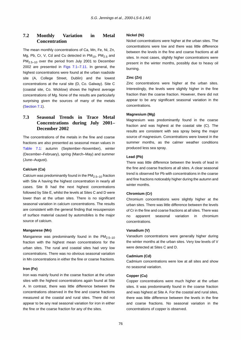
S.G. Jennings et al., 2000-LS-6.1-M1
7.2 Monthly Variation in MetalConcentration
The mean monthly concentrations of Ca, Mn, Fe, Ni, Zn,
Mg, Pb, Cr, V, Cd and Cu detected in PM10, PM2.5 and
PM2.5–10 over the period from July 2001 to December
2002 are presented in Figs 7.1–7.11. In general, the
highest concentrations were found at the urban roadside
site (A, College Street, Dublin) and the lowest
concentrations at the rural site (D, Co. Galway). Site C
(coastal site, Co. Wicklow) shows the highest average
concentrations of Mg. None of the results are particularly
surprising given the sources of many of the metals
(Section 7.1).
7.3 Seasonal Trends in Trace MetalConcentrations during July 2001–December 2002
The concentrations of the metals in the fine and coarse
fractions are also presented as seasonal mean values in
Table 7.1: autumn (September–November), winter
(December–February), spring (March–May) and summer
(June–August).
Calcium (Ca)
Calcium was predominantly found in the PM2.5–10 fraction
with Site A having the highest concentration in nearly all
cases. Site B had the next highest concentrations
followed by Site E, whilst the levels at Sites C and D were
lower than at the urban sites. There is no significant
seasonal variation in calcium concentrations. The results
are consistent with the general finding that resuspension
of surface material caused by automobiles is the major
source of calcium.
Manganese (Mn)
Manganese was predominantly found in the PM2.5–10
fraction with the highest mean concentrations for the
urban sites. The rural and coastal sites had very low
concentrations. There was no obvious seasonal variation
in Mn concentrations in either the fine or coarse fractions.
Iron (Fe)
Iron was mainly found in the coarse fraction at the urban
sites with the highest concentrations again found at Site
A. In contrast, there was little difference between the
concentrations observed in the fine and coarse fractions
measured at the coastal and rural sites. There did not
appear to be any real seasonal variation for iron in either
the fine or the coarse fraction for any of the sites.
Nickel (Ni)
Nickel concentrations were higher at the urban sites. The
concentrations were low and there was little difference
between the levels in the fine and coarse fractions at all
sites. In most cases, slightly higher concentrations were
present in the winter months, possibly due to heavy oil
burning.
Zinc (Zn)
Zinc concentrations were higher at the urban sites.
Interestingly, the levels were slightly higher in the fine
fraction than the coarse fraction. However, there did not
appear to be any significant seasonal variation in the
concentrations.
Magnesium (Mg)
Magnesium was predominantly found in the coarse
fraction and was highest at the coastal site (C). The
results are consistent with sea spray being the major
source of magnesium. Concentrations were lowest in the
summer months, as the calmer weather conditions
produced less sea spray.
Lead (Pb)
There was little difference between the levels of lead in
the fine and coarse fractions at all sites. A clear seasonal
trend is observed for Pb with concentrations in the coarse
and fine fractions noticeably higher during the autumn and
winter months.
Chromium (Cr)
Chromium concentrations were slightly higher at the
urban sites. There was little difference between the levels
of Cr in the fine and coarse fractions at all sites. There was
no apparent seasonal variation in chromium
concentrations.
Vanadium (V)
Vanadium concentrations were generally higher during
the winter months at the urban sites. Very low levels of V
were detected at Sites C and D.
Cadmium (Cd)Cadmium concentrations were low at all sites and show
no seasonal variation.
Copper (Cu)Copper concentrations were much higher at the urban
sites. It was predominantly found in the coarse fraction
and was highest at Site A. For the coastal and rural sites,
there was little difference between the levels in the fine
and coarse fractions. No seasonal variation in the
concentrations of copper is observed.
76
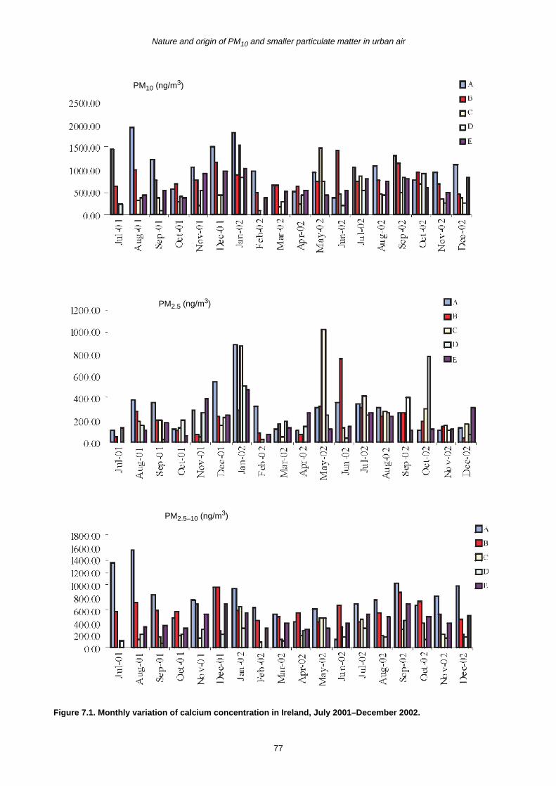
Nature and origin of PM10 and smaller particulate matter in urban air
Figure 7.1. Monthly variation of calcium concentration in Ireland, July 2001–December 2002.
PM2.5–10 (ng/m3)
PM10 (ng/m3)
PM2.5 (ng/m3)
77

S.G. Jennings et al., 2000-LS-6.1-M1
Figure 7.2. Monthly variation of manganese concentration in Ireland, July 2001–December 2002.
PM10 (ng/m3)
PM2.5 (ng/m3)
PM2.5–10 (ng/m3)
78
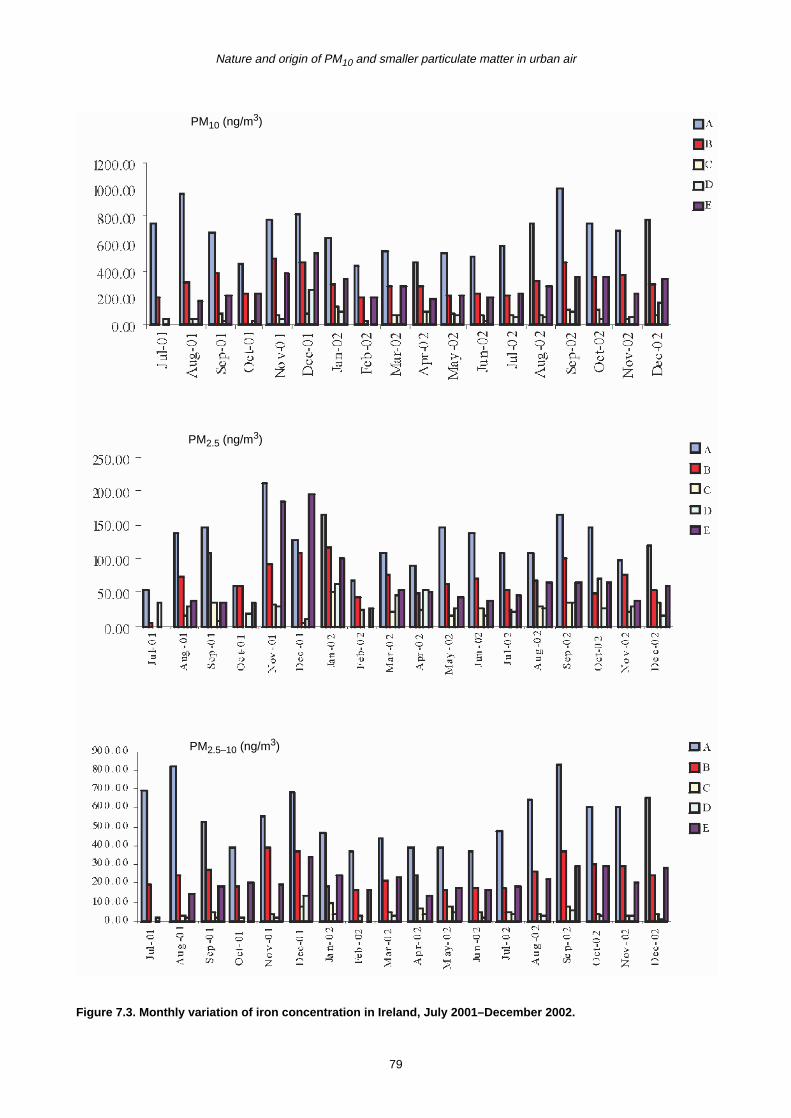
Nature and origin of PM10 and smaller particulate matter in urban air
Figure 7.3. Monthly variation of iron concentration in Ireland, July 2001–December 2002.
PM10 (ng/m3)
PM2.5 (ng/m3)
PM2.5–10 (ng/m3)
79

S.G. Jennings et al., 2000-LS-6.1-M1
Figure 7.4. Monthly variation of nickel concentration in Ireland, July 2001–December 2002.
PM10 (ng/m3)
PM2.5 (ng/m3)
PM2.5–10 (ng/m3)
80

Nature and origin of PM10 and smaller particulate matter in urban air
Figure 7.5. Monthly variation of zinc concentration in Ireland, July 2001–December 2002.
PM10 (ng/m3)
PM2.5 (ng/m3)
PM2.5–10 (ng/m3)
81
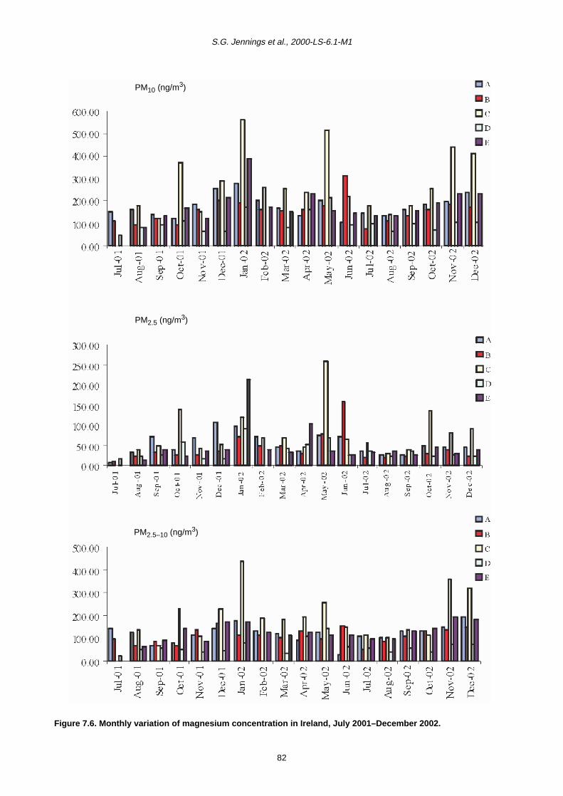
S.G. Jennings et al., 2000-LS-6.1-M1
Figure 7.6. Monthly variation of magnesium concentration in Ireland, July 2001–December 2002.
PM10 (ng/m3)
PM2.5 (ng/m3)
PM2.5–10 (ng/m3)
82

Nature and origin of PM10 and smaller particulate matter in urban air
Figure 7.7. Monthly variation of lead concentration in Ireland, July 2001–December 2002.
PM10 (ng/m3)
PM2.5 (ng/m3)
PM2.5–10 (ng/m3)
83

S.G. Jennings et al., 2000-LS-6.1-M1
Figure 7.8. Monthly variation of chromium concentration in Ireland, July 2001–December 2002.
PM10 (ng/m3)
PM2.5 (ng/m3)
PM2.5–10 (ng/m3)
84

Nature and origin of PM10 and smaller particulate matter in urban air
Figure 7.9. Monthly variation of vanadium concentration in Ireland, July 2001–December 2002.
PM10 (ng/m3)
PM2.5 (ng/m3)
PM2.5–10 (ng/m3)
85
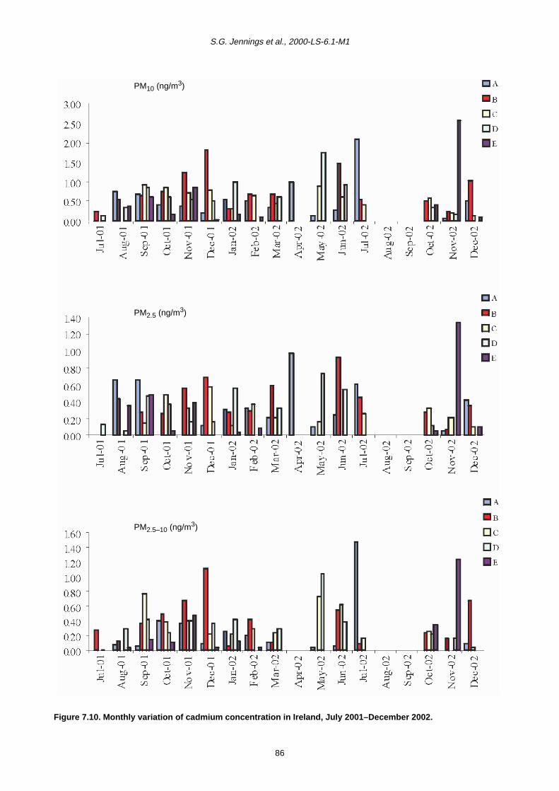
S.G. Jennings et al., 2000-LS-6.1-M1
Figure 7.10. Monthly variation of cadmium concentration in Ireland, July 2001–December 2002.
PM10 (ng/m3)
PM2.5 (ng/m3)
PM2.5–10 (ng/m3)
86
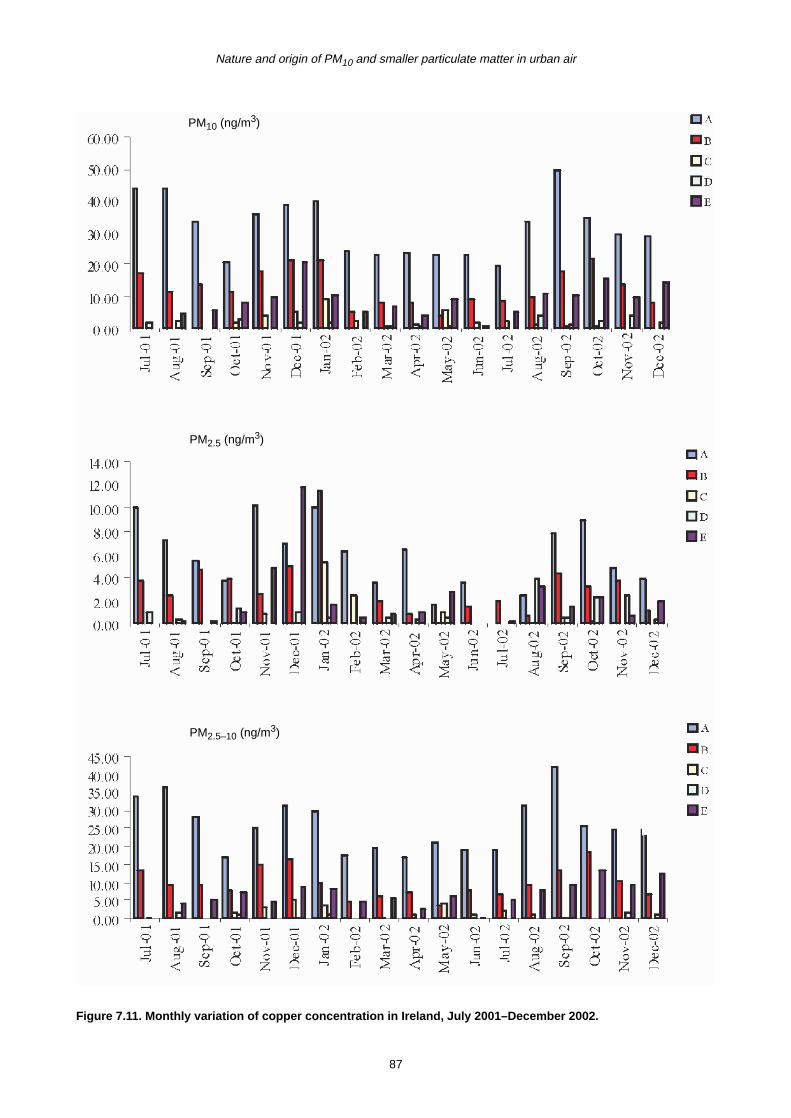
Nature and origin of PM10 and smaller particulate matter in urban air
Figure 7.11. Monthly variation of copper concentration in Ireland, July 2001–December 2002.
PM10 (ng/m3)
PM2.5 (ng/m3)
PM2.5–10 (ng/m3)
87
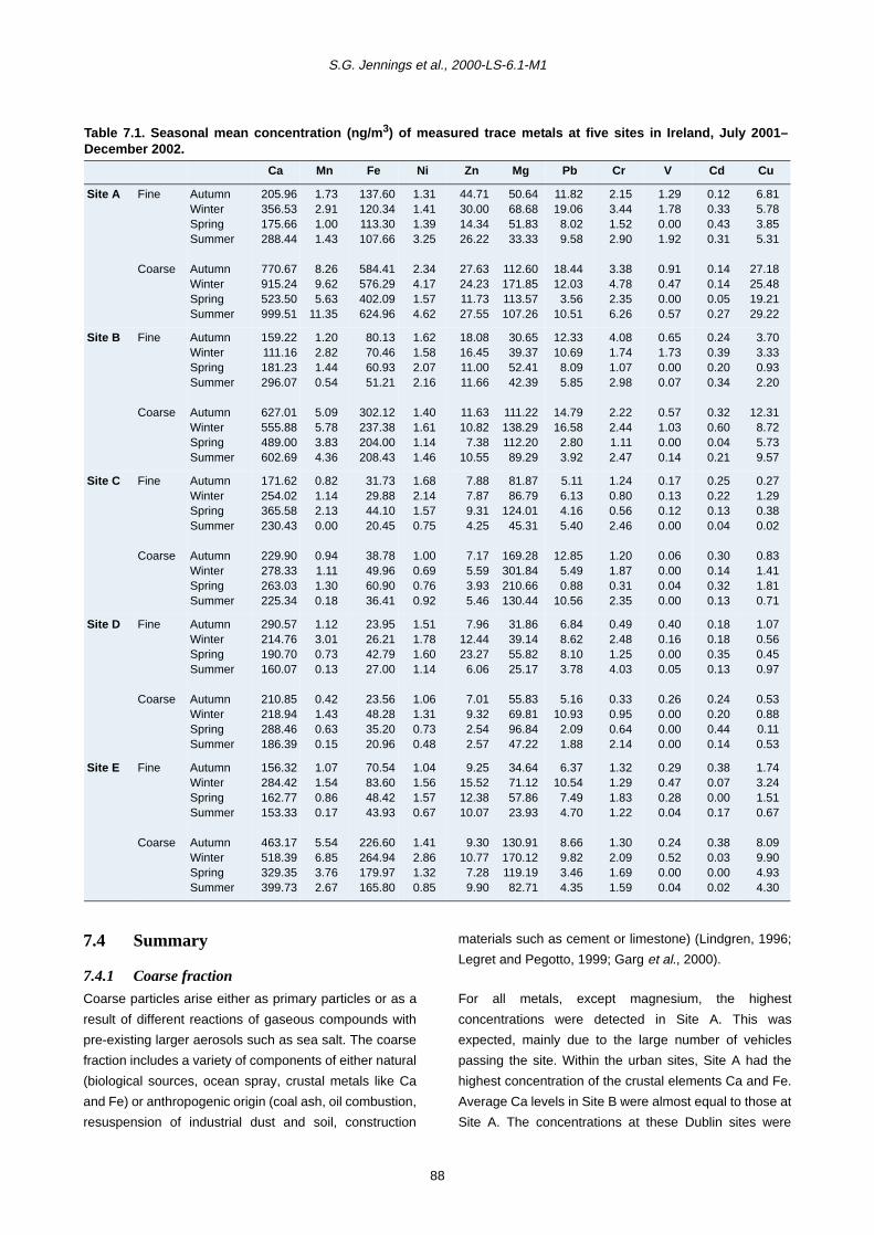
S.G. Jennings et al., 2000-LS-6.1-M1
7.4 Summary
7.4.1 Coarse fraction
Coarse particles arise either as primary particles or as a
result of different reactions of gaseous compounds with
pre-existing larger aerosols such as sea salt. The coarse
fraction includes a variety of components of either natural
(biological sources, ocean spray, crustal metals like Ca
and Fe) or anthropogenic origin (coal ash, oil combustion,
resuspension of industrial dust and soil, construction
materials such as cement or limestone) (Lindgren, 1996;
Legret and Pegotto, 1999; Garg et al., 2000).
For all metals, except magnesium, the highest
concentrations were detected in Site A. This was
expected, mainly due to the large number of vehicles
passing the site. Within the urban sites, Site A had the
highest concentration of the crustal elements Ca and Fe.
Average Ca levels in Site B were almost equal to those at
Site A. The concentrations at these Dublin sites were
Table 7.1. Seasonal mean concentration (ng/m3) of measured trace metals at five sites in Ireland, July 2001–December 2002.
Ca Mn Fe Ni Zn Mg Pb Cr V Cd Cu
Site A Fine
Coarse
AutumnWinterSpringSummer
AutumnWinterSpringSummer
205.96356.53175.66288.44
770.67915.24523.50999.51
1.732.911.001.43
8.269.625.63
11.35
137.60120.34113.30107.66
584.41576.29402.09624.96
1.311.411.393.25
2.344.171.574.62
44.7130.0014.3426.22
27.6324.2311.7327.55
50.6468.6851.8333.33
112.60171.85113.57107.26
11.8219.06
8.029.58
18.4412.03
3.5610.51
2.153.441.522.90
3.384.782.356.26
1.291.780.001.92
0.910.470.000.57
0.120.330.430.31
0.140.140.050.27
6.815.783.855.31
27.1825.4819.2129.22
Site B Fine
Coarse
AutumnWinterSpringSummer
AutumnWinterSpringSummer
159.22111.16181.23296.07
627.01555.88489.00602.69
1.202.821.440.54
5.095.783.834.36
80.1370.4660.9351.21
302.12237.38204.00208.43
1.621.582.072.16
1.401.611.141.46
18.0816.4511.0011.66
11.6310.82
7.3810.55
30.6539.3752.4142.39
111.22138.29112.2089.29
12.3310.69
8.095.85
14.7916.58
2.803.92
4.081.741.072.98
2.222.441.112.47
0.651.730.000.07
0.571.030.000.14
0.240.390.200.34
0.320.600.040.21
3.703.330.932.20
12.318.725.739.57
Site C Fine
Coarse
AutumnWinterSpringSummer
AutumnWinterSpringSummer
171.62254.02365.58230.43
229.90278.33263.03225.34
0.821.142.130.00
0.941.111.300.18
31.7329.8844.1020.45
38.7849.9660.9036.41
1.682.141.570.75
1.000.690.760.92
7.887.879.314.25
7.175.593.935.46
81.8786.79
124.0145.31
169.28301.84210.66130.44
5.116.134.165.40
12.855.490.88
10.56
1.240.800.562.46
1.201.870.312.35
0.170.130.120.00
0.060.000.040.00
0.250.220.130.04
0.300.140.320.13
0.271.290.380.02
0.831.411.810.71
Site D Fine
Coarse
AutumnWinterSpringSummer
AutumnWinterSpringSummer
290.57214.76190.70160.07
210.85218.94288.46186.39
1.123.010.730.13
0.421.430.630.15
23.9526.2142.7927.00
23.5648.2835.2020.96
1.511.781.601.14
1.061.310.730.48
7.9612.4423.27
6.06
7.019.322.542.57
31.8639.1455.8225.17
55.8369.8196.8447.22
6.848.628.103.78
5.1610.93
2.091.88
0.492.481.254.03
0.330.950.642.14
0.400.160.000.05
0.260.000.000.00
0.180.180.350.13
0.240.200.440.14
1.070.560.450.97
0.530.880.110.53
Site E Fine
Coarse
AutumnWinterSpringSummer
AutumnWinterSpringSummer
156.32284.42162.77153.33
463.17518.39329.35399.73
1.071.540.860.17
5.546.853.762.67
70.5483.6048.4243.93
226.60264.94179.97165.80
1.041.561.570.67
1.412.861.320.85
9.2515.5212.3810.07
9.3010.77
7.289.90
34.6471.1257.8623.93
130.91170.12119.1982.71
6.3710.54
7.494.70
8.669.823.464.35
1.321.291.831.22
1.302.091.691.59
0.290.470.280.04
0.240.520.000.04
0.380.070.000.17
0.380.030.000.02
1.743.241.510.67
8.099.904.934.30
88
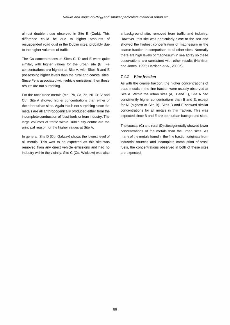
Nature and origin of PM10 and smaller particulate matter in urban air
almost double those observed in Site E (Cork). This
difference could be due to higher amounts of
resuspended road dust in the Dublin sites, probably due
to the higher volumes of traffic.
The Ca concentrations at Sites C, D and E were quite
similar, with higher values for the urban site (E). Fe
concentrations are highest at Site A, with Sites B and E
possessing higher levels than the rural and coastal sites.
Since Fe is associated with vehicle emissions, then these
results are not surprising.
For the toxic trace metals (Mn, Pb, Cd, Zn, Ni, Cr, V and
Cu), Site A showed higher concentrations than either of
the other urban sites. Again this is not surprising since the
metals are all anthropogenically produced either from the
incomplete combustion of fossil fuels or from industry. The
large volumes of traffic within Dublin city centre are the
principal reason for the higher values at Site A.
In general, Site D (Co. Galway) shows the lowest level of
all metals. This was to be expected as this site was
removed from any direct vehicle emissions and had no
industry within the vicinity. Site C (Co. Wicklow) was also
a background site, removed from traffic and industry.
However, this site was particularly close to the sea and
showed the highest concentration of magnesium in the
coarse fraction in comparison to all other sites. Normally
there are high levels of magnesium in sea spray so these
observations are consistent with other results (Harrison
and Jones, 1995; Harrison et al., 2003a).
7.4.2 Fine fraction
As with the coarse fraction, the higher concentrations of
trace metals in the fine fraction were usually observed at
Site A. Within the urban sites (A, B and E), Site A had
consistently higher concentrations than B and E, except
for Ni (highest at Site B). Sites B and E showed similar
concentrations for all metals in this fraction. This was
expected since B and E are both urban background sites.
The coastal (C) and rural (D) sites generally showed lower
concentrations of the metals than the urban sites. As
many of the metals found in the fine fraction originate from
industrial sources and incomplete combustion of fossil
fuels, the concentrations observed in both of these sites
are expected.
89

S.G. Jennings et al., 2000-LS-6.1-M1
8 Polycyclic Aromatic Hydrocarbons (PAHs)
8.1 Sources of PAHs
Polycyclic aromatic hydrocarbons are products of
incomplete combustion formed during the burning of fossil
fuels. They are present in the atmosphere as gases (e.g.
naphthalene), solids adsorbed/absorbed to the surfaces
of fine particles (e.g. benzo(a)pyrene), and semi-volatile
compounds that are partitioned between the gas and
particle phase (e.g. phenanthrene, fluoranthene). The
widespread presence of PAHs in the atmosphere is due
to their emissions from a wide range of combustion
sources including diesel and petrol engines, coal fires,
power stations, biomass burning and incinerators. There
are hundreds of different PAHs, including many
derivatised compounds such as nitro-PAHs. Many of
these compounds are known or suspected carcinogens
and there is currently great concern over the effects of
PAHs on human health. To this end, the US EPA has
selected 16 PAHs as ‘priority pollutants’, based on their
abundance in the atmosphere and known impact on
human health. These compounds are shown in Fig. 8.1.
8.2 Monthly Variation in Concentrationof PAHs
In this work the concentrations of the 16 PAHs were
measured in the fine and coarse fractions collected at the
five sites. The mean monthly concentrations of the PAHs
detected in PM10, PM2.5 and PM2.5–10 over the period
from September 2001–October 2002 are presented in
Figs 8.2–8.14.
Thirteen of the 16 US EPA priority PAH pollutants were
detected in particulate matter collected at the sites. The
concentrations of dibenzo(a,h)anthracene, indeno(1,2,3-
cd)pyrene and benzo(ghi)perylene were below the
detection limits of the method employed in this work. As
expected, the concentration of the PAHs was highest at
the urban sites due to the large number of combustion
Figure 8.1. The 16 US E PA ‘priority PAH pollu tants’.
90

Nature and origin of PM10 and smaller particulate matter in urban air
Figure 8.2. Monthly variation of naphthalene concentration in Ireland, September 2001–October 2002.
PM10 (ng/m3)
PM2.5 (ng/m3)
PM2.5–10 (ng/m3)
91

S.G. Jennings et al., 2000-LS-6.1-M1
sources, especially automobile traffic. The levels of PAHs
were largest at the Dublin roadside (Site A), whilst similar
concentrations were observed at the urban background
sites in Dublin (B) and Cork (E). Very low concentrations
of the PAHs were observed at the coastal and rural sites
due to the lack of significant sources.
The concentrations of the particle-phase PAHs measured
at the five sites are similar to those observed at other
locations around the world (Smith and Harrison, 1998).
The concentration of benzo(a)pyrene is of particular
interest because a threshold value of 1 ng/m3 will be
introduced in 2005 as part of a new EU directive. At Site
A, the monthly average value exceeded this threshold on
five occasions. At Sites B and E, the monthly average
value exceeded this threshold on three and four
occasions, respectively. Further monitoring of
benzo(a)pyrene concentrations is clearly required.
8.3 Trends in PAH Concentration
The first eight PAHs, naphthalene to pyrene, exist
predominantly in the gas phase, although the extent of
partitioning between gas and solid-phase strongly
depends on temperature and the amount of available
surface material. Consequently, the concentrations
measured for these compounds, and in particular the first
four PAHs, are low. Although naphthalene was observed
at all sites, acenaphthylene, acenaphthene and fluorene
were only detected at the urban sites in the autumn and
winter months at very low concentrations. The fact that
these first four PAHs were found predominantly in the
coarse fraction indicates that they probably condensed
onto existing coarse particles in the atmosphere. In
contrast, the five least volatile measured PAHs,
benzo(a)anthracene to benzo(a)pyrene, were detected
mainly in the fine fraction, indicating that they were
probably adsorbed onto particles in the accumulation
Figure 8.3. Monthly variation of acenaphthylene concentration in Ireland, September 2001–October 2002. (Note:
not detected in the PM 2.5 fraction.)
PM2.5–10 (ng/m3)
PM10 (ng/m3)
92

Nature and origin of PM10 and smaller particulate matter in urban air
mode. The remaining four PAHs, phenanthrene,
anthracene, fluoranthene and pyrene, were detected at all
sites with similar concentrations in the fine and coarse
fractions. This is readily understood because these
compounds readily partition between the gas and particle
phases in the atmosphere.
The concentrations of the measured PAHs in the fine and
coarse fractions are also presented as seasonal mean
values in Table 8.1: autumn (September–November),
winter (December–February), spring (March–May) and
summer (June–August). There is a reasonably strong
seasonal variation in the concentration of PAHs. In the
majority of cases, the mean concentrations in the autumn
and winter months were significantly higher than those in
the summer months. This is more clearly seen in the data
for the urban sites. The difference between PAH
concentrations in winter and summer has been attributed
to the following (Smith and Harrison, 1998): (i) increase in
emissions from domestic heating, (ii) winter traffic (from
congestion and cold starts), (iii) meteorological conditions
which favour less pollutant dispersion in winter, and (iv)
possible loss of PAHs due to photochemical decay in
summer.
8.4 Summary
The concentration of the PAHs was highest at the urban
sites due to the large number of combustion sources,
especially automobile traffic. The levels of PAHs were
largest at the Dublin roadside (Site A), whilst similar
concentrations were observed at the urban background
sites in Dublin (B) and Cork (E). Very low concentrations
of the PAHs were observed at the coastal and rural sites
due to the lack of significant sources. The concentrations
of the particle-phase PAHs measured at the five sites are
similar to those observed at other locations around the
Figure 8.4. Monthly variation of acenaphthene concentration in Ireland, September 2001–October 2002. (Note:
not detected in the PM 2.5 fraction.)
PM2.5–10 (ng/m3)
PM10 (ng/m3)
93
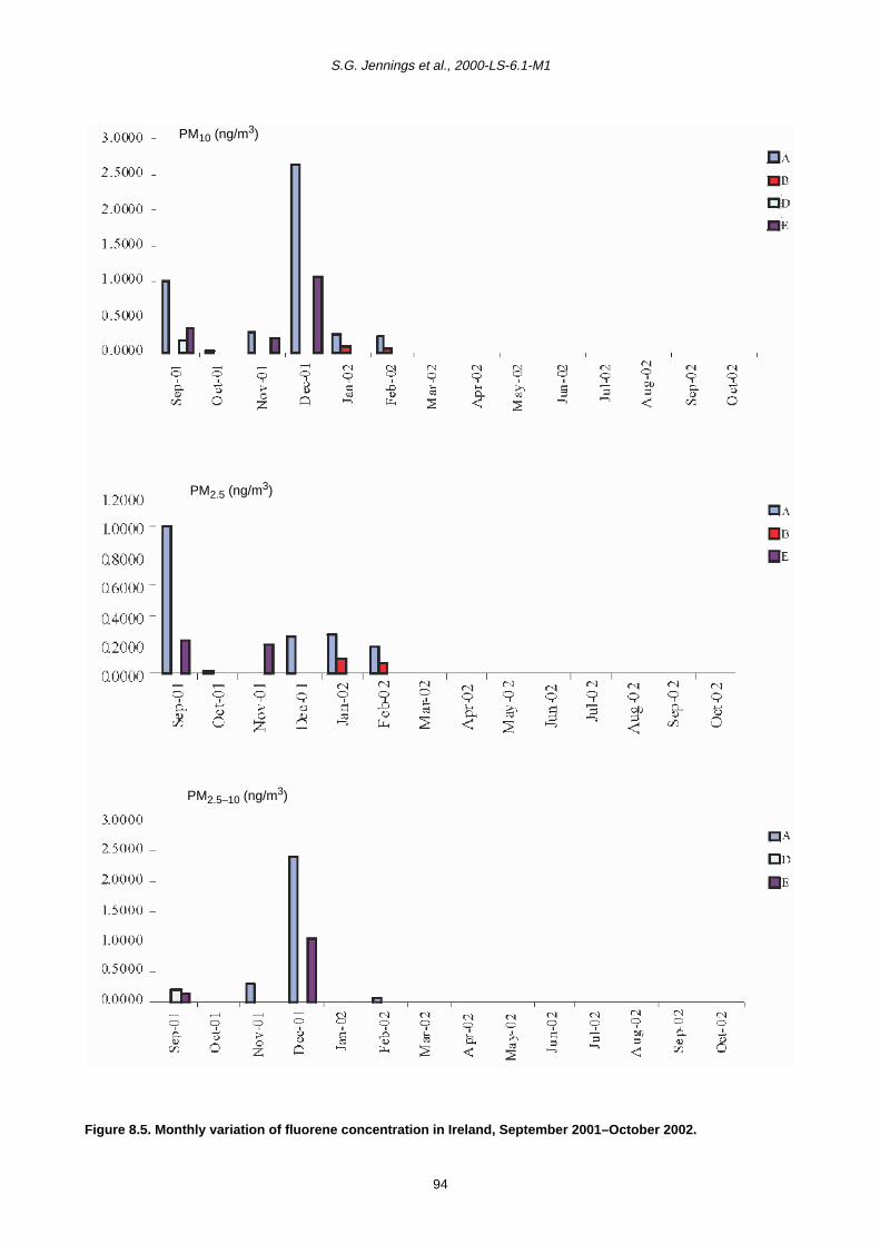
S.G. Jennings et al., 2000-LS-6.1-M1
Figure 8.5. Monthly variation of fluorene concentration in Ireland, September 2001–October 2002.
PM10 (ng/m3)
PM2.5 (ng/m3)
PM2.5–10 (ng/m3)
94
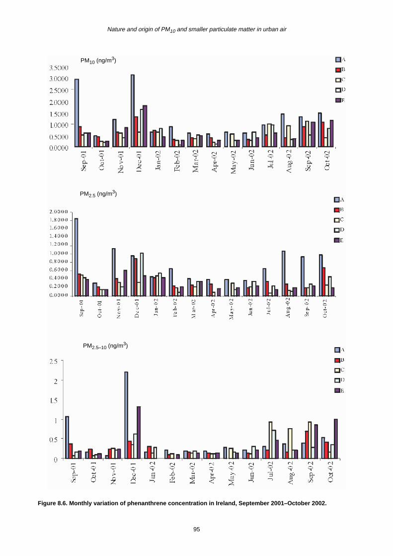
Nature and origin of PM10 and smaller particulate matter in urban air
Figure 8.6. Monthly variation of phenanthrene concentration in Ireland, September 2001–October 2002.
PM10 (ng/m3)
PM2.5 (ng/m3)
PM2.5–10 (ng/m3)
95

S.G. Jennings et al., 2000-LS-6.1-M1
Figure 8.7. Monthly variation of anthracene concentration in Ireland, September 2001–October 2002.
PM10 (ng/m3)
PM2.5 (ng/m3)
PM2.5–10 (ng/m3)
96
Nature and origin of PM10 and smaller particulate matter in urban air
Figure 8.8. Monthly variation of fluoranthene concentration in Ireland, September 2001–October 2002.
PM10 (ng/m3)
PM2.5 (ng/m3)
PM2.5–10 (ng/m3)
97

S.G. Jennings et al., 2000-LS-6.1-M1
Figure 8.9. Monthly variation of pyrene concentration in Ireland, September 2001–October 2002.
PM10 (ng/m3)
PM2.5 (ng/m3)
PM2.5–10 (ng/m3)
98
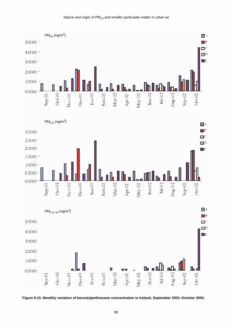
Nature and origin of PM10 and smaller particulate matter in urban air
Figure 8.10. Monthly variation of benzo(a)anthracene concentration in Ireland, September 2001–October 2002.
PM10 (ng/m3)
PM2.5 (ng/m3)
PM2.5–10 (ng/m3)
99
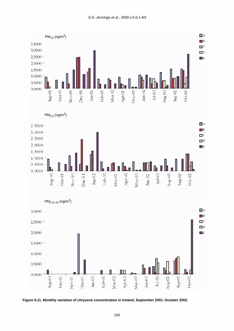
S.G. Jennings et al., 2000-LS-6.1-M1
Figure 8.11. Monthly variation of chrysene concentration in Ireland, September 2001–October 2002.
PM10 (ng/m3)
PM2.5 (ng/m3)
PM2.5–10 (ng/m3)
100
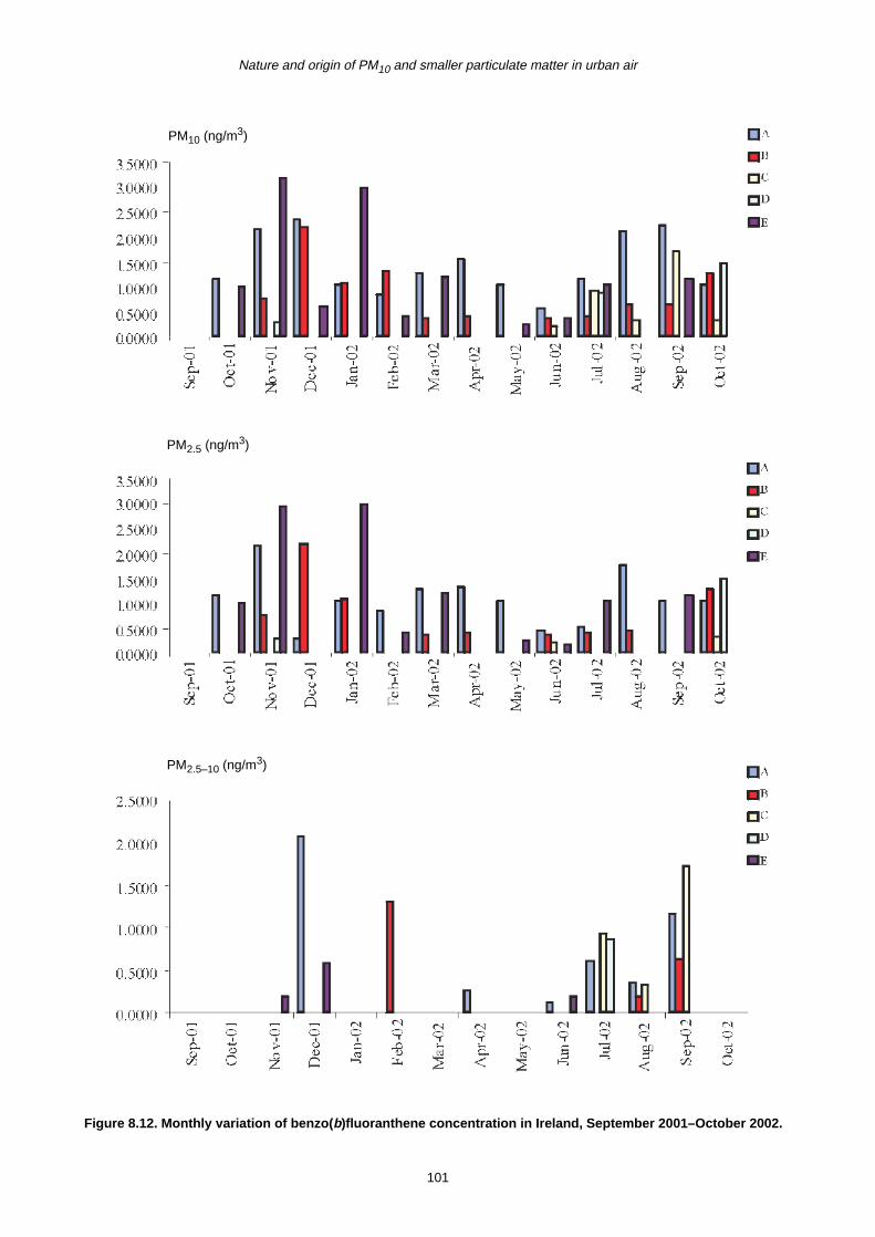
Nature and origin of PM10 and smaller particulate matter in urban air
Figure 8.12. Monthly variation of benzo(b)fluoranthene concentration in Ireland, September 2001–October 2002.
PM10 (ng/m3)
PM2.5 (ng/m3)
PM2.5–10 (ng/m3)
101
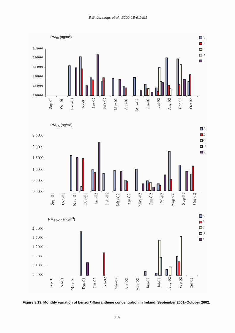
S.G. Jennings et al., 2000-LS-6.1-M1
Figure 8.13. Monthly variation of benzo(k)fluoranthene concentration in Ireland, September 2001–October 2002.
PM10 (ng/m3)
PM2.5 (ng/m3)
PM2.5–10 (ng/m3)
102
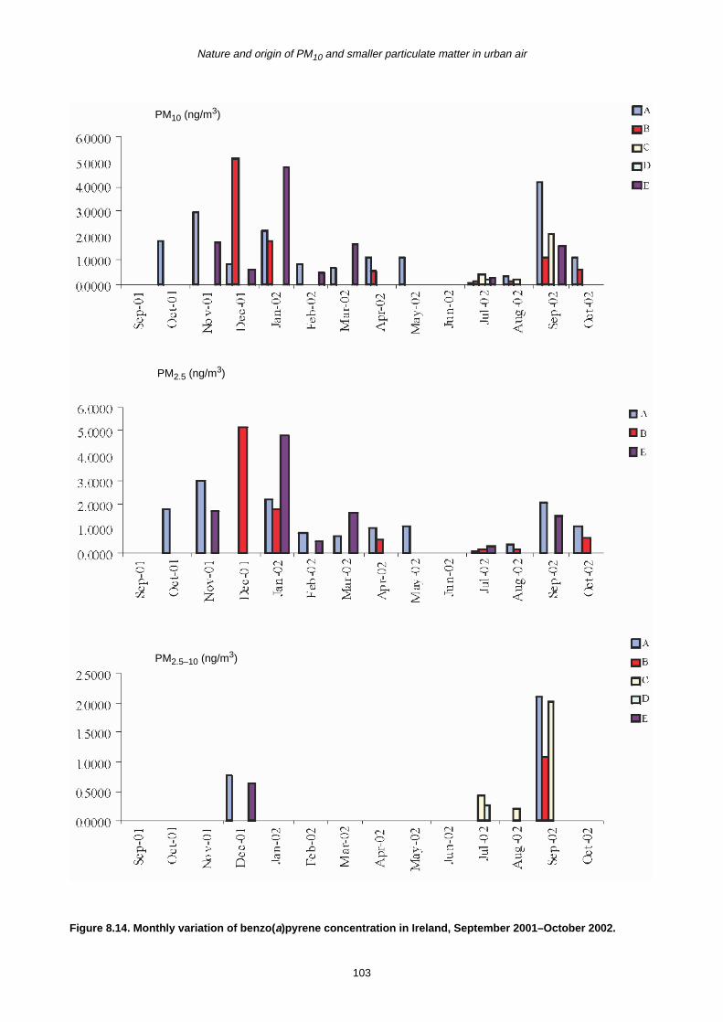
Nature and origin of PM10 and smaller particulate matter in urban air
Figure 8.14. Monthly variation of benzo(a)pyrene concentration in Ireland, September 2001–October 2002.
PM10 (ng/m3)
PM2.5 (ng/m3)
PM2.5–10 (ng/m3)
103
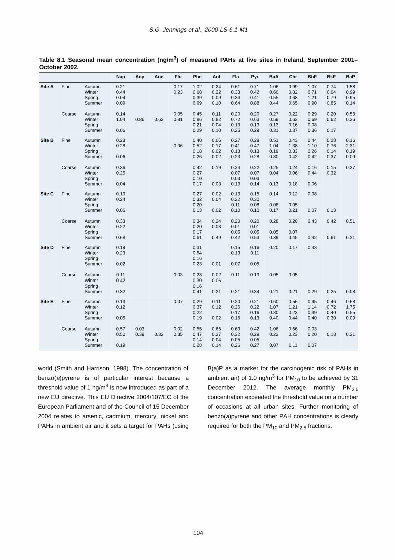
S.G. Jennings et al., 2000-LS-6.1-M1
world (Smith and Harrison, 1998). The concentration of
benzo(a)pyrene is of particular interest because a
threshold value of 1 ng/m3 is now introduced as part of a
new EU directive. This EU Directive 2004/107/EC of the
European Parliament and of the Council of 15 December
2004 relates to arsenic, cadmium, mercury, nickel and
PAHs in ambient air and it sets a target for PAHs (using
B(a)P as a marker for the carcinogenic risk of PAHs in
ambient air) of 1.0 ng/m3 for PM10 to be achieved by 31
December 2012. The average monthly PM2.5
concentration exceeded the threshold value on a number
of occasions at all urban sites. Further monitoring of
benzo(a)pyrene and other PAH concentrations is clearly
required for both the PM10 and PM2.5 fractions.
Table 8.1 Seasonal mean concentration (ng/m3) of measured PAHs at five sites in Ireland, September 2001–October 2002.
Nap Any Ane Flu Phe Ant Fla Pyr BaA Chr BbF BkF BaP
Site A Fine
Coarse
AutumnWinterSpringSummer
AutumnWinterSpringSummer
0.210.440.040.09
0.141.04
0.06
0.86 0.62
0.170.23
0.050.81
1.020.680.390.69
0.450.860.210.29
0.240.220.090.10
0.110.820.040.10
0.610.330.340.64
0.200.720.130.25
0.710.420.410.88
0.200.630.130.29
1.060.600.550.44
0.270.590.130.31
0.990.820.630.65
0.220.630.160.37
1.070.711.210.90
0.290.690.080.36
0.740.640.790.85
0.200.62
0.17
1.580.990.950.14
0.530.26
Site B Fine
Coarse
AutumnWinterSpringSummer
AutumnWinterSpringSummer
0.230.28
0.06
0.360.25
0.04
0.060.400.520.180.26
0.420.270.100.17
0.060.170.020.02
0.19
0.03
0.270.410.130.23
0.240.070.030.13
0.280.470.130.28
0.220.070.030.14
0.511.040.190.30
0.250.04
0.13
0.431.380.330.42
0.240.06
0.18
0.441.100.260.42
0.160.44
0.06
0.280.760.140.37
0.150.32
0.162.310.190.09
0.27
Site C Fine
Coarse
AutumnWinterSpringSummer
AutumnWinterSpringSummer
0.190.24
0.06
0.330.22
0.68
0.270.320.200.13
0.340.200.170.61
0.020.04
0.02
0.240.03
0.49
0.130.220.110.10
0.200.010.050.42
0.150.300.080.10
0.200.010.050.53
0.14
0.080.17
0.28
0.050.39
0.12
0.050.21
0.20
0.070.45
0.08
0.07
0.43
0.42
0.13
0.42
0.61
0.51
0.21
Site D Fine
Coarse
AutumnWinterSpringSummer
AutumnWinterSpringSummer
0.190.23
0.02
0.110.42
0.32
0.03
0.310.540.160.23
0.230.300.160.41
0.01
0.020.06
0.21
0.150.13
0.07
0.11
0.21
0.160.11
0.05
0.13
0.34
0.20
0.05
0.21
0.17
0.05
0.21
0.43
0.29 0.25 0.08
Site E Fine
Coarse
AutumnWinterSpringSummer
AutumnWinterSpringSummer
0.130.12
0.05
0.570.50
0.19
0.030.39 0.32
0.07
0.020.35
0.290.370.220.19
0.550.470.140.28
0.110.12
0.02
0.650.370.040.14
0.200.260.170.16
0.630.320.050.26
0.210.220.160.13
0.420.290.050.27
0.601.070.300.40
1.060.22
0.07
0.561.210.230.44
0.660.23
0.11
0.951.140.490.40
0.030.20
0.07
0.460.720.400.30
0.18
0.681.750.550.09
0.21
104

Nature and origin of PM10 and smaller particulate matter in urban air
9 General Conclusions and Recommendations for FutureWork
9.1 General Conclusions
i. PM10 levels in Ireland lie within the range of other
European countries and are similar to those in the
neighbouring UK, but with a more marked maritime
influence seen in higher sea salt concentrations in
the coarse particle mode.
ii. Concentrations of PM10 and PM2.5 at urban locations
in Ireland were around four times the rural
background, and at the roadside were around six
times the rural background and often exceeded the
current EU limits. This indicates the importance of
road traffic as a source. There was a large urban
increment in carbonaceous aerosols and
resuspended dusts due to the rapid pace of
development in the transport, energy and
building/road construction sectors.
iii. Similar urban PM concentrations and variations were
found in both Dublin and Cork, indicative of national
uniformity of urban aerosol concentrations and
behaviour, with concurrent episodes of elevated
PM10 mostly being associated with increased levels
of finer particles consisting of both local and long-
range transported components. The highest PM
levels were often associated with polluted
UK/European air masses, when both local and long-
range transported sources can be significant.
iv. In non-urban areas, high PM10 levels were
influenced mainly by sea salt and secondary
particles possessing a significant long-range
transport component. On the other hand, mainly
local sources dominate higher levels of PM during
advection of clean westerly air masses.
v. Mass closure analysis explained 79–93% of the fine
particle mass and 72–81% of the coarse particle
mass, depending on location. In urban areas, the
predominant components of fine particles are
organics, EC and secondary inorganics, and the
main components of coarse particles are
resuspended materials and sea salt.
vi. In non-urban areas, PM2.5 mostly consists of
secondary inorganic and organic materials whilst
sea salt contributes the most to coarse fractions.
Uncertainties are likely to have arisen from
underestimation of resuspended materials (at urban
sites) and organics (at non-urban sites), as well as
the presence of water within hygroscopic aerosols.
vii. The levels of PAHs were largest at the Dublin city
roadside site, whilst similar concentrations were
observed at the urban background sites in Dublin
and Cork due to the large number of combustion
sources. Very low concentrations of the PAHs were
observed at the coastal and rural sites due to the lack
of significant sources. The concentrations of the
particle-phase PAHs measured at the five sites are
similar to those observed at other locations around
the world.
viii. Mass closure procedures using reconstructed
chemical components were used to identify major
source categories contributing to the aerosol mass,
namely primary marine aerosol (NaCl), secondary
inorganic materials (NH4NO3 + (NH4)2SO4), primary
anthropogenic combustion materials (EC), primary
and secondary organic materials, and resuspended
dusts. Source component contributions differed for
fine and coarse particles and at different locations.
ix. In urban areas, the major components contributing to
fine particle mass (together accounting for 79–84%
of PM2.5 mass) were, in order, organic compounds,
EC, ammonium sulphate/ammonium nitrate, whilst in
the coarse fraction resuspended material and sea
salt were predominant (56–66%).
x. Chemical component (using secondary aerosol
components of sulphate, nitrate and ammonium)
analysis according to air mass origin from data in
Chapter 5 indicates that long-range transport from
an eastwardly direction – mainly from the continent
and the UK – to Dublin (Site B) accounts for up to
about 30% of the PM2.5 mass (as a fraction of the
total mass) over and above that measured under
105

S.G. Jennings et al., 2000-LS-6.1-M1
westerly or maritime air mass conditions, and up to
about 25% of the PM10 mass.
xi. Results show that local sources contribute 50% or
more to fine PM mass (PM2.5) and to coarse PM
(PM10) for the city centre sites.
xii. At the rural and coastal sites, PM2.5 mainly consisted
of ammonium sulphate/ammonium nitrate and
organic materials (65%), whilst sea salt was the
largest contributor to coarse particles (39% rural,
56% coastal). Unexplained materials, accounting for
about 7–28% of the mass, were attributed mainly to
resuspended materials at urban sites and organic
materials at the other sites, as well as unmeasured
water content.
xiii. The levels of PAHs were largest at the Dublin
roadside (Site A), whilst similar concentrations were
observed at the urban background sites in Dublin (B)
and Cork (E) due to the large number of combustion
sources. Very low concentrations of the PAHs were
observed at the coastal and rural sites due to the lack
of significant sources. The concentrations of the
particle-phase PAHs measured at the five sites are
similar to those observed at other locations around
the world.
xiv. The highest concentrations for all metals, except
magnesium, for both the coarse and fine fractions,
were obtained at the kerbside Dublin city centre site.
In general, the rural site in Co. Galway shows the
lowest level for all metals. The coastal site showed
the highest concentration of magnesium in the
coarse fraction in comparison to the other four sites.
The coastal and rural sites generally showed lower
fine fraction concentrations of the metals than at the
urban sites.
xv. Intensive measurements carried out during 4 weeks
in February–March 2002 showed, on average, that
chemical species concentrations measured for the
size-resolved impactor samples are very similar to
those measured for the daily samples. Reasonable
agreement (generally within 25%) was obtained
between cumulative gravimetric mass from week-
long MOUDI impactor samples and individual daily
samples over the same week. Largest disagreement
(up to 50%) was found at the rural site, which is
largely due to relatively low levels at the site.
xvi. These measurements represent the first
comprehensive air quality PM10, PM2.5 and PM2.5–10
assessment in Ireland, coupled with quite detailed
chemical composition data.
9.2 Recommendations for Future Work
i. It is strongly recommended that the future air quality
programme should also include size-differentiated
mass and size-differentiated chemical composition
data. This could be facilitated by means of an
extended EMEP activity at some selected sites.
ii. Very few PM2.5 samplers are employed and there is
need for the establishment of collocated PM2.5 and
PM10 monitors since increasing emphasis (by EMEP
for example) is being given to lower sized particulate
sampling in view of associated health effects.
iii. The monitoring of background baseline data on a
more continuous basis is considered to be important,
particularly in view of the more stringent EU limit
values coming into operation in January 2010.
iv. Mass closure needs to be achieved between PM10,
PM2.5 mass and the sum of PM components. The
high percentage of unresolved mass (of order 40%)
is thought to be mainly due to unaccounted OC.
v. Air quality sampling programmes should include
measurement of ultrafine particles as they have
been shown to be more toxic per unit mass than
coarse sized particles. Therefore, measurement of
number concentration levels of ultrafine particles
should accompany conventional PM mass and
chemical sampling.
vi. Particular PAHs, such as benzo(a)pyrene, are of
particular interest because, as from 31 December
2012, in accordance with a new EU directive (EU
Directive 2004/107/EC), concentrations of
benzo(a)pyrene, used as a marker for PAHs in
ambient air, must not exceed a target value of 1
ng/m3 for PM10. Such species should be monitored
on a routine basis in anticipation of new directives
involving the fine or PM2.5 fraction.
vii. Further work on determination of the main source
contributors to mass concentrations of PM10 (and
PM2.5) is recommended.
106

Nature and origin of PM10 and smaller particulate matter in urban air
10 References
Allen, A., Nemitz, E., Shi, J.P., Harrison, R.M. and Greenwood,J.C., 2001. Size distribution of trace metals in atmosphericaerosols in the United Kingdom. Atmospheric Environment35: 4581–4591.
APEG, 1999. Source Apportionment of Airborne ParticulateMatter in the United Kingdom. Report of the AirborneParticle Expert Group, DETR, UK.
Bardouki, H., Liakakou, H., Economou, C., Sciare, J., Smolík, J.,dímal, V., Eleftheriadis, K., Lazaridis, M., Dye, C. and
Mihalopoulos, N., 2003. Chemical composition of size-resolved atmospheric aerosols in the eastern Mediterraneanduring summer and winter. Atmospheric Environment 37:195–208.
Borbely-Kiss, I., Koltay, E., Szabo, G., Bozo L. and Tar, T., 1999.Composition and sources of urban and rural atmosphericaerosol in eastern Hungary. Journal of Aerosol Science30(3): 369–391.
Bowman, F.M., Odum, J.R., Seinfeld, J.H. and Pandis, S.N.,1997. Mathematical model for gas-particle partitioning ofsecondary organic aerosols. Atmospheric Environment 31:3921–3931.
Castro, L.M., Pio, C.A., Harrison, R.M. and Smith, D.J.T., 1999.Carbonaceous aerosol in urban and rural Europeanatmospheres: estimation of secondary organic carbonconcentrations. Atmospheric Environment 33: 2771–2781.
Ceburnis, D., Yin, J., Allen, A.G., Jennings, S.G., Harrison, R.M.,Wright, E., Fitzpatrick, M., Healy, T. and Barry, E., 2006.Local and regional air pollution in Ireland during an intensiveaerosol measurement campaign. Journal of EnvironmentalMonitoring 8: 479–487.
Chan, Y.C., Simpson, R.W., McTainsh, G.H., Vowles, P.D.,Cohen, D.D. and Bailey, G.M., 1997. Characterisation ofchemical species in PM2.5 and PM10 aerosols in Brisbane,
Australia. Atmospheric Environment 31: 3773–3785.
Chow, J.C., Watson, J.G., Fujita, E.M., Lu, Z. and Lawson, D.R.,1994. Temporal and spatial variations of PM2.5 and PM10
aerosol in the Southern California Air Quality Study.Atmospheric Environment 28: 2061–2080.
Cohen, D., Stelcer, E. and Garton, D., 2002. Ion beam methodsto determine trace heavy metals concentrations and sourcesin urban airsheds. Nuclear Instruments and Methods inPhysics Research B190: 466–470.
Dockery, D.W., Pope, C.A., Xu, X.P., Spengler, J.D., Ware, J.H.,Fay, M.E., Ferris, B.G. and Speizer, F.E., 1993. Anassociation between air pollution and mortality in six U.S.cities. New England Journal of Medicine 329: 1753–1759.
Eldred, R.A., Cahill, T.A. and Floccini, R.G., 1997. Compositionof PM2.5 and PM10 aerosols in the IMPROVE network.
Journal of the Air and Waste Management Association 47:194–203.
EPA, 2000. Ireland’s Environment – A Millennium Report. EPA,Johnstown Castle Estate, Co. Wexford, Ireland.
EU Council Air Quality Framework Directive 1999/30/EC –http://europa.eu.int/comm/environment/air/ambient.htm,1999.
Garg, B., Cadle, S.H., Mulawa, P.A., Groblicki, P.J., Laroo, C.and Parr, G.A., 2000. Brake wear particulate matteremissions. Environmental Science and Technology 34:4463–4469.
Gelencsér, A., Hoffer, A., Krivácsy, Z., Kiss, G., Molnár, A. andMészáros, E., 2002. On the possible origin of humic matterin fine continental aerosol. Journal of Geophysical Research107: doi2001JD001299.
Harrison, R.M. and Jones, M., 1995. The chemical compositionof airborne particles in the UK atmosphere. Science of theTotal Environment 168: 195–214.
Harrison, R.M., Msibi, I.M., Kitto, A.M.N. and Yamulki, S., 1994.Atmospheric chemical transformations of nitrogencompounds measured in the North Sea experiment.Atmospheric Environment 28: 1593–1599.
Harrison, R.M., Yin, J., Mark, D., Stedman, J., Appleby, R.S.,Booker, J. and Moorcroft, S., 2001. Studies of the coarseparticle (2.5–10 µm) component in UK urban atmospheres.Atmospheric Environment 35: 3667–3679.
Harrison, R.M., Tilling, R., Callen Romero, M., Harrad, S. andJarvis, K., 2003a. A study of trace metals and polycyclicaromatic hydrocarbons in the roadside environment.Atmospheric Environment 37: 2391–2402.
Harrison, R.M., Jones, A.M. and Lawrence, R.G., 2003b. Apragmatic mass closure model for airborne particulatematter at urban background and roadside sites.Atmospheric Environment 37: 4927–4933.
Horvath, H., 1993. Atmospheric light absorption – a review.Atmospheric Environment 27A: 293–317.
Horvath, H., 1997. Experimental calibration for aerosol lightabsorption measurement using the integrating plate method– summary of the data. Journal of Aerosol Science 28:1149–1161.
Horvath, H., Kasahara, M. and Pesava, P., 1996. The sizedistribution and composition of the atmospheric aerosol at arural and nearby urban location. Journal of Aerosol Science27: 417–435.
Jalkanen, L. and Hasanen, E., 1996. Simple method for thedissolution of atmospheric aerosol samples for analysis byinductively coupled plasma mass spectrometry. Journal ofAnalytical Atomic Spectrometry 11: 365–369.
Jennings, S.G., O’Dowd, C.D., O’Connor, T.C. and McGovern,F.M., 1991. Physical characteristics of the ambient aerosolat Mace Head. Atmospheric Environment 25A: 557–562.
Jennings, S.G, Kleefeld, C., O’Dowd, C., Junker, C., Spain, T.G.,O’Brien, P., Roddy, A.F. and O’Connor, T.C., 2003. MaceHead Atmospheric Research Station – characterization ofaerosol radiative parameters. Boreal EnvironmentalResearch 8: 303–314.
Jones, M.R., 1996. Physical and Chemical Properties of
107

S.G. Jennings et al., 2000-LS-6.1-M1
Airborne Particulate Matter in Birmingham, UK. Ph.D. thesis.The University of Birmingham.
Keary, J., Jennings, S.G., O’Connor, T.C., McManus, B. and Lee,M., 1998. PM10 concentration measurements in Dublin City.
Environmental Monitoring and Assessment 52: 3–18.
Kim, B.M., Teffera, S. and Zeldin, M.D., 2000. Characterizationof PM2.5 and PM10 in the South Coast Air Basin of Southern
California: Part 1 – spatial variations. Journal of the Air andWaste Management Association 50: 2034–2044.
Legret, M. and Pegotto, C., 1999. Evaluation of pollutantloadings in the runoff waters from a major rural highway.Science of the Total Environment 235: 143–150.
Lindgren, A., 1996. Asphalt wear and pollution transport.Science of the Total Environment 190: 281–286.
Luhana, L., 1995. Source Apportionment of Particulate Matterover Birmingham Using Receptor Models. Ph.D. thesis. TheUniversity of Birmingham, UK.
Morandi, M.T., Daisey, J.M. and Lioy, P.J., 1987. Development ofa modified factor analysis/multiple regression model toapportion suspended particulate matter in a complex urbanairshed. Atmospheric Environment 21: 1821–1831.
Müller, K., 1999. A three year study of aerosol in northwestSaxony (Germany). Atmospheric Environment 33: 1679–1685.
O'Dowd, C.D., Facchini, M.C., Cavalli, F., Ceburnis, D., Mircea,M., Decesari, S., Fuzzi, S., Yoon, Y.J. and Putaud, J.P.,2004. Biogenically-driven organic contribution to marineaerosol. Nature 431: 676–680.
Pandis, S.N., Harley, R.A., Cass, G.R. and Seinfeld, J.H., 1992.Secondary organic aerosol formation and transport.Atmospheric Environment 26A: 2269–2282.
Pope, C.A., Schwartz, J. and Ransom, M.R., 1992. Dailymortality and PM10 pollution in Utah Valley. Archives of
Environmental Health 47: 211–217.
QUARG, 1996. Airborne Particulate Matter in the UK. ThirdReport of the Quality of Urban Air Review Group.Department of the Environment, London.
Robache, A., Mathe, F., Galloo, J.C. and Guillermo, R., 2000.Multi-element analysis by inductively coupled plasma opticalemission spectrometry of airborne particulate mattercollected with a low-pressure cascade impactor. Analyst125: 1855.
Schmid, H., Laskus, L., Abraham, H.J., Baltensperger, U., et al.,2001. Results of the ‘carbon conference’ internationalaerosol carbon round robin test stage I. AtmosphericEnvironment 35: 2111–2121.
Schwartz, J., Dockery, D.W. and Neas, L.M., 1996. Is dailymortality associated specifically with fine particles? Journalof the Air and Waste Management Association 46: 927–939.
Seinfeld, J.H. and Pandis, S.N., 1998. Atmospheric Chemistryand Physics. John Wiley and Sons, Inc., New York, 1326 pp.
Smith, D.J.T. and Harrison, R.M., 1998. Polycyclic aromatichydrocarbons in atmospheric particles. In: Harrison, R.M.and Van Grieken, R. (eds) Atmospheric Particles. JohnWiley and Sons, pp. 253–294.
Speer, R.E., Edney, E.O. and Kleindienst, T.E., 2003. Impact oforganic compounds on the concentrations of liquid water inambient PM2.5. Journal of Aerosol Science 34: 63–77.
Spokes, L., Jickells, T. and Jarvis, K., 2001. Atmospheric inputsof trace metals to the northeast Atlantic Ocean: theimportance of southeasterly flow. Marine Chemistry 76:319–330.
Stedman, J.R., 1997. The Secondary Particle Contribution toElevated PM10 Concentrations in the UK. AEA Technology,
National Environmental Technology Centre. Report20008001/007.
Stedman, J.R., Linehan, E. and Conlan, B., 2001. Receptormodelling of PM10 concentrations at a United Kingdom
national network monitoring site in central London.Atmospheric Environment 35: 297–304.
Turnbull, A.B. and Harrison, R.M., 2000. Major componentcontributions to PM10 composition in the UK atmosphere.
Atmospheric Environment 34: 3129–3137.
Turpin, B.J. and Lim, H.J., 2001. Species contributions to PM2.5
mass concentrations: Revising common assumptions forestimating organic mass. Aerosol Science and Technology35: 602–610.
Yin, J., 2002. Monitoring of Airborne Particulate Mass andNumber Concentrations in the UK Atmosphere. Ph.D.thesis. The University of Birmingham.
Yin, J., Allen, A.G., Jennings, S.G., Harrison, R.M., McGovern,F., Wright, E., Fitzpatrick, M., Healy, T., Barry, E., Ceburnis,D. and McCusker, D., 2005. Major component compositionof urban PM10 and PM2.5 in Ireland. Atmospheric Research
78: 149–165.
108


![[PPT]Environmental Chemistry - PowerPoint … · Web viewAtmospheric Chemistry Formation of the Atmosphere The Early Atmosphere Origin of Life and Oxygen Ozone Air Pollution Acid](https://static.fdocuments.net/doc/165x107/5b0b179c7f8b9a45518d6ccd/pptenvironmental-chemistry-powerpoint-viewatmospheric-chemistry-formation-of.jpg)