Air Pollution Modelling and Its Application
561
Transcript of Air Pollution Modelling and Its Application

Air PollutionModeling and ItsApplication XV

Previous Volumes in this Mini-Series
Volumes I–XII were included in the NATO Challenges of Modern Society Series.
AIR POLLUTION MODELING AND ITS APPLICATION IEdited by C. De Wispelaere
AIR POLLUTION MODELING AND ITS APPLICATION IIEdited by C. De Wispelaere
AIR POLLUTION MODELING AND ITS APPLICATION IIIEdited by C. De Wispelaere
AIR POLLUTION MODELING AND ITS APPLICATION IVEdited by C. De Wispelaere
AIR POLLUTION MODELING AND ITS APPLICATION VEdited by C. De Wispelaere, Francis A. Schiermeier, and Noor V. Gillani
AIR POLLUTION MODELING AND ITS APPLICATION VIEdited by Han van Dop
AIR POLLUTION MODELING AND ITS APPLICATION VIIEdited by Han van Dop
AIR POLLUTION MODELING AND ITS APPLICATION VIIIEdited by Han van Dop and Douw G. Steyn
AIR POLLUTION MODELING AND ITS APPLICATION IXEdited by Han van Dop and George Kallos
AIR POLLUTION MODELING AND ITS APPLICATION XEdited by Sven-Erik Gryning and Millán M. Millán
AIR POLLUTION MODELING AND ITS APPLICATION XIEdited by Sven-Erik Gryning and Francis A. Schiermeier
AIR POLLUTION MODELING AND ITS APPLICATION XIIEdited by Sven-Erik Gryning and Nadine Chaumerliac
AIR POLLUTION MODELING AND ITS APPLICATION XIIIEdited by Sven-Erik Gryning and Ekaterina Batchvarova
AIR POLLUTION MODELING AND ITS APPLICATION XIVEdited by Sven-Erik Gryning and Francis A. Schiermeier

Air PollutionModeling and ItsApplication XV
Edited by
Carlos BorregoUniversity of AveiroAveiro, Portugal
and
Guy SchayesCatholic University of LouvainLouvain-la-Neuve, Belgium
KLUWER ACADEMIC PUBLISHERSNEW YORK, BOSTON, DORDRECHT, LONDON, MOSCOW

eBook ISBN: 0-306-47813-7Print ISBN: 0-306-47294-5
©2004 Kluwer Academic PublishersNew York, Boston, Dordrecht, London, Moscow
Print ©2002 Kluwer Academic/Plenum Publishers
All rights reserved
No part of this eBook may be reproduced or transmitted in any form or by any means, electronic,mechanical, recording, or otherwise, without written consent from the Publisher
Created in the United States of America
Visit Kluwer Online at: http://kluweronline.comand Kluwer's eBookstore at: http://ebooks.kluweronline.com
New York

In 1969 the North Atlantic Treaty Organization (NATO) established the Committee onChallenges of Modern Society (CCMS). The subject of air pollution was from the start, oneof the priority problems under study within the framework of various pilot studies undertakenby this committee. The organization of a periodic conference dealing with air pollutionmodelling and its application has become one of the main activities within the pilot studyrelating to air pollution. These international conferences were successively organized by theUnited States (first five); Federal Republic of Germany (five); Belgium (five); TheNetherlands (four) and Denmark (five). With this one Portugal takes over the duty.
This volume contains the papers and poster abstracts presented at theNATO/CCMS International Technical Meeting on Air Pollution Modelling and ItsApplication held in Louvain-la-Neuve, Belgium, during 15-19 October 2001. This ITM wasjointly organized by the University of Aveiro, Portugal (Pilot country) and by the CatholicUniversity of Louvain, Belgium (host country).
The ITM was attended by 78 participants representing 26 countries from Western andEastern Europe, North and South America, Asia, Australia and Africa. The main topics ofthis ITM were : Role of Atmospheric Models in Air Pollution Policy and AbatementStrategies; Integrated Regional Modelling; Global and Long-Range Transport; Regional AirPollution and Climate; New Developments; and Model Assessment and Verification.
Invited papers were presented by A. Ebel of Germany (Changing atmosphericenvironment, changing views); H. ApSimon of Great Britain (Applying risk assessmenttechniques to air pollution modelling & abatement strategies); and S.E. Gryning of Denmark(Aspects of meteorological pre-processing of fluxes over inhomogeneous terrain).
On behalf of the Scientific Committee and as organizers and editors, we should like toexpress our gratitude to all participants who made the meeting so successful, resulting in thepublication of this book. The efforts of the chairpersons and rapporteurs were especiallyappreciated. Thanks also to the teams of Aveiro and Louvain-la Neuve that managed allpractical matters adequately.
Finally special thanks are due to the sponsoring institutions: NATO/CCMS: Committeeon the Challenges of Modern Society; University of Aveiro, Portugal; Catholic University ofLouvain, Belgium; FNRS: Fonds National de la Recherche Scientifique, Belgium;EURASAP: European Association for the Sciences of Air Pollution; ICCTI: Institute forInternational Scientific and Technological Cooperation, Portugal.
NATO/CCMS grants allowed attendance from Central and Eastern Europe. The nextconference in this series will be held in 2003 in Istanbul (Turkey).
PREFACE
Guy SCHAYESLocal Conference OrganizerBelgium
Carlos BORREGOScientific Committee ChairpersonPortugal
v

This page intentionally left blank

THE MEMBERS OF THE SCIENTIFIC COMMITTEE FOR THENATO/CCMS INTERNATIONAL TECHNICAL MEETINGS ON AIRPOLLUTION MODELLING AND ITS APPLICATION
Schayes, BelgiumD. Syrakov, BulgariaD. Steyn, CanadaS.-E. Gryning, DenmarkN. Chaumerliac, FranceE. Renner, GermanyG. Kallos, GreeceD. Anfossi, Italy
P. Builtjes, The NetherlandsT. Iversen, NorwayC. Borrego, Portugal (Chairman)J.M. Baldasano, SpainS. Incecik, TurkeyB. Fisher, United KingdomF. Schiermeier, USAY. Schiffman, USA
vii

This page intentionally left blank

ix
HISTORY OF THE NATO/CCMS AIR POLLUTION PILOT STUDIES
Pilot Study on Air Pollution: International Technical Meetings (ITM)on Air Pollution Modelling and Its Application
Dates of Completed Pilot Studies:
1969 - 1974 Air Pollution Pilot Study (United States)1975 - 1979 Air Pollution Assessment Methodologies and Modelling (Germany)1980 - 1984 Air Pollution Control Strategies and Impact Modelling (Germany)
Dates and Locations of Pilot Study Follow-Up Meetings:
Pilot Country – United States (R.A. McCormick, L.E. Niemeyer)
February 1971 – Eindhoven, The Netherlands, First Conference on Low Pollution PowerSystems Development
July 1971 – Paris, France, Second Meeting of the Expert Panel on Air PollutionModelling
All of the following meetings were entitled NATO/CCMS International TechnicalMeetings (ITM) on Air Pollution Modelling and Its Application
October 1972 – Paris, France - Third ITMMay 1973 – Oberursel, Federal Republic of Germany - Fourth ITMJun 1974 – Roskilde, Denmark- Fifth ITM
Pilot Country – Germany (Erich Weber)
September 1975 – Frankfurt, Federal Republic of Germany – Sixth ITMSeptember 1976 – Airlie House, Virginia, USA – Seventh ITMSeptember 1977 – Louvain-La-Neuve, Belgium – Eighth ITMAugust 1978 – Toronto, Ontario, Canada – Ninth ITMOctober 1979 – Rome, Italy – Tenth ITM
Pilot Country – Belgium (C. De Wispelaere)
November 1980 – Amsterdam, The Netherlands – Eleventh ITM

August 1981 – Menlo Park, California, USA – Twelfth ITMSeptember 1982 – Ile des Embiez, France – Thirteenth ITMSeptember 1983 – Copenhagen, Denmark – Fourteenth ITMApril 1985 – St. Louis, Missouri, USA – Fifteenth ITM
Pilot Country – The Netherlands (Han van Dop)
April 1987 – Lindau, Federal Republic of Germany – Sixteenth ITMSeptember 1988 – Cambridge, United Kingdom – Seventeenth ITMMay 1990 – Vancouver, British Columbia, Canada – Eighteenth ITMSeptember 1991 – lerapetra, Crete, Greece – Nineteenth ITM
Pilot Country – Denmark (Sven-Erik Gryning)
November 1993 – Valencia, Spain - Twentieth ITMNovember1995 – Baltimore, Maryland, USA – Twenty-First ITMJune 1997 – Clermont-Ferrand, France – Twenty-Second ITMSeptember 1998 – Varna, Bulgaria – Twenty-Third ITMMay 2000 – Boulder, Colorado, USA – Twenty-Fourth (Millennium) ITM
Pilot Country – Portugal (Carlos Borrego)
October 2001 – Louvain-la-Neuve, Belgium – Twenty-Fifth ITM
x
CONTENTS
ROLE OF ATMOSPHERIC MODELS IN AIR POLLUTION POLICYAND ABATEMENT STRATEGIES
xi
A policy oriented model system for the assessment of long-termeffects of emission reductions on ozone
C. Mensink, L. Delobbe and A. Colles
Transforming deterministic air quality modeling results intoprobabilistic form for policy-making
S. T. Rao and Ch. Hogrefe
INTEGRATED REGIONAL MODELLING
Changing atmospheric environment, changing views – and anair quality model’s response on the regional scale
A. Ebel
Development of a regional model for ozone forecasting and acidicdeposition mapping
A. Tang, N. Reid and P. K. Misra
Modelling of Atmospheric radioactive aerosol dynamics and depositionA. Baklanov and A. Aloyan
Air quality study over the Atlantic coast of Iberian peninsulaAna C. Carvalho, Anabela Carvalho, A. Monteiro, C. Borrego,
A.I. Miranda, I.R. Gelpi, V. Pérez-Muñuzuri, M.R. Méndez and J.A. Souto
Numerically simulated atmospheric transboundary contribution of leadloading to the Great Lakes
S. M. Daggupaty and J. Ma
3
13
25
37
45
59
69
189
On the coupling of air-pollution model to numerical weatherprediction model
T. Halenka, J. Brechler and J. Bednar
Modeling the mercury cycle in the Mediterranean: similaritiesand differences with conventional air pollution modeling
G. Kallos, A. Voudouri, I. Pytharoulis and O. Kakaliagou
The Australian air quality forecasting system: Modelling of asevere smoke event in Melbourne, Australia
S. Lee, M. Cope, K. Tory, D. Hess and Y.L. Ng
Pre-processor for regional-scale fluxes and mixed-layer heightover inhomogeneous terrain
S.-E. Gryning and E. Batchvarova
Validation of urban air quality modelling in the European UnionP. Suppan and A. Skouloudis
Development and application of chemical weather forecasting systemover East Asia
I. Uno, K. Ishihara, Z. Wang, G.R. Carmichael and M. Baldi
Photo-oxidation processes over the Eastern Mediterranean basin in summerM. Varinou, F. Gofa, G. Kallos, M. O’Connor and G. Tsiligiridis
Numerical study of tropospheric ozone in the spring time in East AsiaM. Zhang, I. Uno, Z. Wang and H. Akimoto
Testing smog indices using a comprehensive modelCh. Fung, H-Ch. Lau, L. Yu, K. Leung and A. Chang
An application of a photochemical model for urban airshed in IstanbulS. Topcu and S. Incecik
One-way nesting versus two-way nesting: does it really make a difference ?C. Soriano, O. Jarbo and J. M. Baldasano
GLOBAL AND LONG-RANGE TRANSPORT
Applying risk assessment techniques to air pollution modelling &abatement strategies
H.M. ApSimon, R.F. Warren and A. Mediavilla-Sahagun
79
87
95
105
115
125
137
147
157
167
177
xii
ETEX simulations with the DMI-HIRLAM numerical weatherprediction model
J. Chenevez, A. Baklanov and J. H. Sørensen
Impact assessment of growing Asian megacity emissionsS. K. Guttikunda, J.J. Yienger, N. Thongboonchoo, G.R. Carmichael,
H. Levy II and D. G. Streets
Transboundary exchange of sulfur pollution in the region of SE EuropeD. Syrakov and M. Prodanova
REGIONAL AIR POLLUTION AND CLIMATE
concentrations over Europe, combining satellite dataand modelling
M. van Loon, P. Builtjes and G. de Leeuw
Simulating soil-dust, sea-salt and sulfate aerosols in East Asiausing RAMS-online chemical transport model coupled withCAM (Canadian aerosol module)
Z. Wang, I. Uno, S. Gong, M. Zhang and H. Akimoto
NEW DEVELOPMENTS
Data assimilation for CT-modelling based on optimum interpolationJ. Flemming, E. Reimer and R. Stern
Inclusion of an improved parameterisation of the wet deposition processin an atmospheric transport model
N. Fournier, K. J. Weston, M. A. Sutton and A. J. Dore
Modeling of urban air pollution: principles and problemsE. Genikhovich, I. Gracheva and E. Filatova
Modelling cloud chemistry in a regional aerosol model: bulk vs.size resolved representation
W. Gong
Parameterisation of turbulence-enhanced nucleation in large scale models:conceptual study
O. Hellmuth and J. Helmert
Models-3/community multiscale air quality (CMAQ) modeling system:2001 Java-based release
S. LeDuc and S. Fine
201
211
221
233
243
255
265
275
285
295
307
xiii

Fuzzy sets application for estimation of air polluted zoneA. Dudatiev, Y. Podobna, P. Molchanov and T. Holyeva
Initial application of the adaptive grid air quality modelM.T. Odman, M. Khan, R. Srivastava and D. Scott McRae
Application of inverse modeling and sensitivity theory to airpollution studies
V. Penenko
Sensitivity analysis of nested photochemical simulationsI. Kioutsioukis, and A.N. Skouloudis
Revisiting ozone-precursor relationshipsB. Ainslie and D. G. Steyn
On the relationship between the Lagrangian and Eulerian timescale: a preliminary evaluation with LES data
U. Rizza, D. Anfossi, C. Mangia and G. A. Degrazia
New Algorithms for the determination of solar radiation, surfacetemperature and PBL height in CALMET
G. Maffeis, R. Bellasio, J. S. Scire, M. G. Longoni,R. Bianconi and N. Quaranta
Use of neutral networks in the field of air pollution modellingM. Z. Boznar and P. Mlakar
A porosity/drag approach for the modeling of flow and dispersion inthe urban canopy
B. Carissimo and R. W. Macdonald
Improved algorithms for advection and vertical diffusion in AURORAK. De Ridder and Cl. Mensink
MODEL ASSESSMENT AND VERIFICATION
Comparison of results from a higher order closure dispersion modelwith measurements in a complex terrain
B. J. Abiodun and L. Enger
Parameterisation of SBL height in atmospheric pollution modelsA. Baklanov
311
319
329
337
347
357
365
375
385
395
405
415
xiv
Evaluation of mixing height parameterization for air pollution modelsL. Delobbe, O. Brasseur, J. Matthijsen, C. Mensink,
F. J. Sauter, G. Schayes and D. P. J. Swart
Using Fuzzy numbers to treat predictions from more than one modelB. Fisher and M. Ireland
NARSTO model comparison and evaluation study (NMCES)D. A. Hansen
Influence of underlying surface roughness to the deposition ofairborne particles in northern winter conditions
M. Kaasik
A study of dispersion around a thermoelectric power plant inthe south of Brazil
O. L. L. Moraes, R. C. M. Alves, R. Silva, A. C. Siqueira,P. D. Borges, T Tirabassi and U. Rizza
A global-Through urban scale nested air pollution modellingsystem (MM5-CMAQ): application to Madrid area
R. San José, J. L. Perez, J. I. Peña, I. Salas and R. M. González
Estimates of uncertainty in urban air quality model predictionsS. Vardoulakis, B. Fisher, N. Gonzalez-Flesca and K. Pericleous
Effects of input data errors on some indices for statistical model evaluationA. Wellens
POSTER SESSION
Assessment of pollution impact over Turin suburban area usingintegrated methods
G. Tinarelli, S. Alessandrini, D. Anfossi, F. Pavone and S. Cuffini
Assessing uncontrolled emissions near a lead worksG. Cosemans and E. Roekens
Design for meteorological monitoring for air pollution modelingin industrial zone of Pancevo, based on experiences during bombing
Z. Grsic, P. Milutinovic, M. Jovasevic-Stojanovic and M. Popovic
The optimal choice of AERMOD input data in complex areasG. Latini, C. Grifoni, and G. Passerini
425
435
445
455
465
473
483
493
505
507
509
513
xv
The Black Triangle area - Fit for Europe? Numerical air quality studiesfor the Black Triangle area
E. Renner, W. Schröder, D. Theiss and R. Wolke
Surface layer turbulence during the total solar eclipse of 11 August 1999G. Schayes, J.L. Mélice and V. Dulière
Seasonal simulation of the air quality in East Asia using CMAQS. Sugata
The role of energy sources of different types in atmospheric pollutionand heat supply options in Irkutsk city
S. P. Filippov and A. V. Keiko
Transport sensitivity analysis on ozone concentrations in IberianPeninsula by using MM5-CMAQ modelling system
R. San José, J. L. Pérez, I. Salas and R. M. Gonzalez
Development of the emission inventory system for supportingTRACE-P and ACE-ASIA field experiments
J.-H. Woo, D. G. Streets, G. R. Carmichael, J. Dorwart,N. Thongboonchoo, S. Guttikunda and Y. Tang
515
517
519
521
525
527
529
541
543
xvi
PARTICIPANTS
AUTHOR INDEX
SUBJECT INDEX

ROLE OF ATMOSPHERIC MODELS IN AIR POLLUTION POLICY ANDABATEMENT STRATEGIES
Chairperson :
Rapporteur :
B. Fisher
Ph. Thunis

This page intentionally left blank

A POLICY ORIENTED MODEL SYSTEM FOR THEASSESSMENT OF LONGTERM EFFECTS OF
EMISSION REDUCTIONS ON OZONE
Clemens Mensink, Laurent Delobbe and Ann Colles*
1. INTRODUCTION
For the evaluation of ozone abatement measures, modelling tools predicting thelong-term effect of emission reductions on ground level ozone are indispensable. In theFlanders region in Belgium such an evaluation is carried out on periodically on a 5-yearbase1 with time horizons set at 5 to 10 years ahead. In general, policy makers express intheir abatement strategies the combination of economic projections and a set of possibleor optional policy measures. Under various sets of constraints, like health effects, socialacceptance, costs and economical feasibility, the problem can be reduced to anoptimisation problem and as a result the most efficient measures are selected, e.g. byapplying multi-criteria analysis2. One of the challenges with respect to policy support forozone abatement is to offer a tool that can provide assessments at low computationalcost. In this way a large number of scenarios can be evaluated within a limited timeframe.
In terms of its effect, ozone exposure is to be assessed on a long-term base,depending on the evaluation variable that is examined. Moreover the formation anddegradation of ozone can cover several days and the transport of ozone and its precursorsis not limited to any national border. These considerations should be taken into accountby the evaluation instrument as well.
We present a tool that has been designed for the assessment of abatement scenarios.It is applied to calculate the long-term effects of European emission reductions on ozonein Belgium. The model system is based on the results of extensive calculations by two airquality models and uses fast multiple linear regression techniques as proposed and usedin the RAINS model3 for the preparation of the recent Gothenburg protocol and ECnational emission ceilings. A first regression model, called OZON94 is based on theresults (5 model scenario runs) of the LOTOS model4 for the summer period of 1994(1 May – 31 August). OZON94 uses the meteorological conditions of the period May-
* Flemish Institute for Technological Research (Vito), Boeretang 200, B-2400 Mol, Belgium.
Air Pollution Modeling and Its Application XV, Edited byBorrego and Schayes, Kluwer Academic/Plenum Publishers, New York, 2002 3
August 1994 and only varies the emissions of the ozone precursors and VOC) in 37European countries. In function of the selected abatement scenario the model calculatesvarious ozone indicators in 15 grid cells covering Belgium. A second regression model iscalled OZON97. It is based on the results (5 runs) of the EUROS model5 for the summerperiod of 1997 (1 May – 30 September) and works in a similar way as OZON94
Various indicators can evaluate the effect of abatement measures on ground levelozone. These indicators are usually based on hourly ozone concentrations that arelocation dependent. In this study, five different ozone parameters are used to evaluateabatement measures: AOT60, NET60 and ADM as indicators for the protection ofhuman health against ozone exposure, and AOT40_f and AOT40_v as indicators for theeffects on forests and on crops and semi-natural vegetation. Their definitions as used inthis study are given below:
AOT60 = Accumulated exposure Over a Threshold of 60 ppb, based on hourlyvalues for the period considered;NET60 = Number of days with a maximum 8-hourly value Exceeding aThreshold of 60 ppb for the period considered;ADM = Average of the Daily Maximum 8-hourly value for the periodconsidered;AOT40_f = Accumulated exposure Over a Threshold of 40 ppb for forests,based on hourly values between 8h and 20h MET from 1 April to 30 September;AOT40_v = Accumulated exposure Over a Threshold of 40 ppb for crops andsemi-natural vegetation, based on hourly values between 8h and 20h MET from1 May to 31 July.
Note that, except for the AOT40_v, these definitions are confined to the periods forwhich meteorological data were available, i.e. between 1 May and 31 August forOZON94 and between 1 May and 30 September for OZON97.
Each of these 5 indicators is used to evaluate a reference situation (1990) and twoemission reduction scenario’s for 2010. The first one is a business as usual (BAU)scenario in which reduction plans and legislative actions are included, before the nationalemission ceilings provided by the Gothenburg protocol were adopted. This scenariocorresponds to the REF scenario belonging to the H1 scenario in the seventh IIASAinterim report6. A second scenario reflects the national emission ceilings (NEC) asprescribed by the UN/ECE 1999 Gothenburg protocol7 to abate acidification,eutrophication and ground-level ozone. It sets emission ceilings for 2010 forVOC and as negotiated on the basis of scientific assessment of pollution effects andabatement options.
Section 2 gives an overview of the methodology and the main elements of the modelsystem. It describes briefly how the equations for the regression model have been derivedand how the model results set the basis to resolve the coefficients that are used toestimate the long-term ozone effect of the emission scenario’s. In section 3 the resultsfor the two scenario’s are presented and discussed. In addition a comparison is madebetween the OZON97 results and the results of the EUROS model, both applied for theemissions prescribed by the NEC scenario. This allows an estimation of the accuracy ofthe regression model with regard to the scenario calculations for the 5 indicators.
4

2. METHODOLOGY
The methodology of the model system consists of the following steps:
Computation of the hourly ozone concentrations for 15 grid cells coveringBelgium for 5 different emission scenarios (base case, -30% -30% VOC, -30% & VOC) and –50% & VOC)) with the LOTOS model for thesummer period of 1994 (1 May – 31 August) to obtain the basis for theOZON94 regression model.Computation of the hourly ozone concentrations for 15 grid cells coveringBelgium for the same 5 emission scenarios with the EUROS model for thesummer period of 1997 (1 May – 30 September) to obtain the basis for theOZON97 regression model.Determination of the regression coefficients for each of the 5 indicators in eachof the 15 grid cells by solving a system of 5 equations with 5 unknowns usingthe ozone calculations performed by LOTOS for OZON94 and by EUROS forOZON97.Computation of the 5 indicators in each of the 15 grid cells by applying theregression model for the 1990 reference case and the BAU and NEC scenario’susing the country based and VOC emission variations as an input.Aggregation of the 15 grid cell values into one value for Belgium by weightedaveraging.
In a next section, the successive steps of the methodology are explained. The resultsfrom the LOTOS (long-term ozone simulation) model were obtained from Builtjes andBoersen4. LOTOS is an Eulerian grid model8 with a horizontal grid resolution ofapproximately and 4 vertical layers extending to 2-3 km. The modelcomputations were performed on a grid containing 70 x 70 grid cells covering a domainfrom 35°N to 70°N and from 10°W to 60°E. Transport phenomena on a regional scale aswell as background concentrations on a continental scale are taken into account by themodel. The photochemical processes in the model are driven by a slightly modifiedversion of the Carbon Bound IV mechanism8.
The EUROS (European Smog) model was developed at RIVM in the Netherlandsand is also applied for long-term ozone calculations5. A detailed description of theEUROS model is given by van Loon9. It is also an Eulerian grid model that covers thewhole of Europe with a spatial resolution of approximately but a gridrefinement procedure allows refinement of the spatial resolution in certain areas of themodel domain, for example in areas where strong concentration gradients occur. The(photo)-chemical module is the recent version of the Carbon Bound IV mechanism10.It includes 32 chemical species and 87 reactions.
Using the hourly ozone concentrations computed by the LOTOS and the EUROSmodel, the impact of the emission scenarios on the 5 indicators was calculated by meansof a multiple linear regression technique as proposed by Amman et al.3:
1.
2.
3.
4.
5.
5

Where:
= the calculated values for the indicator 1 (1=1…5) at receptor j= back ground contribution to the at receptor j= linear contribution of the VOC emissions from country i to receptor j= linear contribution of the emissions from country i to receptor j= non-linear contribution of the emissions from country i to receptor j= non-linear contribution of “effective” emissions (natural sources)= non-linear contribution due to the interactions between and VOC
The “effective” emissions are defined as:
Where:
= a meteorologically dependent variable= the “effective” natural emissions at receptor j
It is assumed that the “effective” natural emissions for the 15 receptor points inBelgium are negligible, certainly when compared to the anthropogenic contributions. Bythis assumption equation (2) is reduced to a (non-linear) quadratic contribution in(1) which can be attributed to the term The last term in equation (1) is replacedby the product of the and VOC contributions multiplied by the coefficient Thisleads to the following expression:
For 15 receptor points located in Belgium (j=1...15) the coefficientsand are determined for the contribution of each emitting country (i=1...37). Thesecontributions are weighted by means of the source-receptor matrices provided byEMEP11. The 5 unknown coefficients in expression (3) are resolved by 5 equationsrelated to 5 situations for which the IND and the and VOC emissions are known(base case and 4 reduction scenarios: -30% -30% VOC, -30% & VOC) and-50% & VOC)). Once the coefficients are calculated they are used to calculate theIND values for 1990 and the BAU and NEC emission scenarios.
An average value for Belgium is obtained by applying weighted averaging. For theAOT60, NET60 and AMD this is based on population density per grid cell. For theAOT40_f the forest density per grid cell is used. For the AOT40_v the cultivatedagricultural area per grid cell is used.
6
3. RESULTS AND DISCUSSION
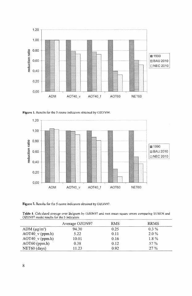
Figure 1 shows the results of the OZON94 regression model for the 5 indicators(ADM, AOT40_v, AOT40_f, AOT60 and NET60). Results are presented for three cases:1990, the BAU scenario in 2010 (BAU 2010) and the NEC scenario in 2010 (NEC2010). For each column in Figure 1, the value of the indicator is divided by the value forthe reference situation in 1990. Thus the relative reduction ratios are presented. In asimilar way Figure 2 shows the results for OZON97. The results of OZON94 andOZON97 cannot be compared by their absolute values, since different meteorologicaldata and different evaluation periods were used. This should also be borne in mind whencomparing the relative reduction ratios. However one can clearly see that both resultsshow the same trend. The average values (ADM) are hardly changing or even show avery slight increase in the case of OZON97. The indicators with a low cut off asthreshold value (AOT40) are only slightly decreasing. This means that backgroundconcentrations seem to have a tendency to rise in the future. On the other hand, theindicators that reflect the maximum values (e.g. AOT60 and NET60) do decreasesignificantly for both models. The difference between AOT60 and NET60 seems toindicate that the amount of ozone excess is decreasing faster than the number of days onwhich the exceedances occur. As a result it can be put forward that the emissionreduction efforts seem to be effective to avoid exceedances rather than to reducebackground levels.
These trends are more or less confirmed by observations in Flanders between 1989and 199912. The measured annual average of the daily maximum 8-hourly values (AMD)shows a rising trend with 4% per year since 1991, indicating an increasing backgroundconcentration. The measured 5-year sliding average of the AOT40_v shows a very slightdecrease (5-10%) over the period 1993-1999. The measured trends for NET60 andAOT60 are less clear. Their values depend strongly on the annual fluctuations insunshine and temperature. However, one should be careful in comparing these trends.The total emissions in Europe for and VOC have decreased with 28% and 23%respectively over the period 1989-1999, whereas in the scenario calculations thereduction rates for the and VOC emissions are 48% and 50% respectively between1990 and 2010. Since the methodology is expected to be very sensitive to different
ratios, a very detailed sensitivity study would be needed to confirm themeasured trends.
In order to estimate the accuracy of the regression method, in particular of theOZON97 method, the results for the NEC scenario were compared with the results of theEUROS model for the same input data. Figure 3 shows the comparison for the 15 gridlocations in Belgium for the AOT40_v. Figure 4 shows the comparison for the AOT60.Table 1 gives the average value of the OZON97 results and the absolute and relativeRMS errors for the 5 indicators, when comparing the grid cell values with the EUROSresults. It can be seen that the regression method performs well for the ADM, theAOT40_v and the AOT40_f, but is more sensitive with respect to AOT60 and NET60.This is obvious, since in some of the grid cells, the levels of AOT60 are close or justbelow the threshold value. Notice also that the OZON97 model gives a systematicunderestimation of the AOT60 compared to the EUROS results for the NEC scenario.
7
8

9

4. CONCLUSIONS
A methodology has been presented for the assessment of long-term effects ofemission reductions on ozone concentrations in Belgium at low computational costs.Results for various scenarios show some important trends. The average values (ADM)are hardly changing or show a slight decrease. The indicators with a low cut off asthreshold value (AOT40) show a slight decrease. Both trends are confirmed byobservations between 1989 and 1999. Indicators representing peak values (e.g. NET60and AOT60) decrease significantly for the various policy scenarios. From themeasurements these trends are not clear, since the annual variation are dominated by thevarying meteorological conditions. For the scenario’s considered the regression methodgives accurate results for the ADM and AOT40 indicators, but less accurate results forthe AOT60 and NET60 indicators.
5. REFERENCES
VMM (2000) MIRA-S 2000: Report on the environment and nature in Flanders: scenarios, Summary,Vlaamse Miliaumaatschappij & Garant, Leuven/Apeldoorn.De Vlieger, I.,Berloznik, R, Duerinck, J. and Mensink, C. (2001) Multidisciplinary study on reducing airpollution from transport. Methodology and emission results, Proceedings of the InternationalConference on Urban Transport and the Environment for the Century, 14-16 May 2001, Lemnos,Greece, WITpress, Southapmton, pp. 429-440.Amann M., Bertok, I., Cofala J., Gyarfas F., Heyes C., Klimont Z., en Schöpp W. (1999) IntegratedAssessment Modelling for the Protocol to Abate Acidification, Eutrophication and Ground-level Ozone inEurope, IIASA, Laxenburg.Builtes P.J.H. en Boersen G. (1996) Model calculations to determine the influence of European emissionreductions on ozone concentrations over Belgium, TNO-report TNO-MEP-R 96/274, Apeldoorn.Matthijsen, J., Delobbe, L., Sauter, F. and de Waal, L. (2001) Changes of surface ozone over Europe uponthe Gothenburg protocol abatement of 1990 reference emissions, Proceedings of the EUROTRAC-2Symposium 2000, Computational Mechanics Publications ( to appear).Amann, M., Bertok, I., Cofala, J., Gyarfas, F., Heyes, C., Klimont, Z., Makowski, M., Schöpp, W. & Syri,S. (1999) Cost-effective control of acidification and ground-level ozone, seventh interim report. IIASA,Laxenburg.UN/ECE (2000) http://www.unece.org/env/lrtap/Builtjes, P.J. H. (1992) The LOTOS Long Term Ozone Simulation-project, Summary Report, TNO-reportTNO-MW-R 92/240, ApeldoornLoon M. van (1996) Numerical methods in smog prediction, PhD thesis, University of Amsterdam.Adelman Z.A. (1999) A re-evaluation of the Carbon Bond-IV photochemical mechanism, Thesis Msr.Sc., Chapel Hill.EMEP (1998) http://www.emep.int/ozone/webo3sr/Dumont, G. and Mensink, C (2000) Photochemical air pollution, in: M. Van Steertegem et al. (eds.),MIRA-S 2000: Report on the environment and nature in Flanders: scenarios, VlaamseMiliaumaatschappij & Garant, Leuven/Apeldoorn (in Dutch), pp. 395-409.
1.
2.
3.
4.
5.
6.
7.8.
9.10.
11.12.
10

DISCUSSION
A. HANSEN
C. MENSINK
Have the results of the LOTOS and regression models beencompared with observational data ?There appears to be certain degree of faith placed in the regressionmodel results.
The results of the LOTOS model for 1994 have been compared withobserved values for the northern part of Belgium (Flanders region)as reported in reference 12 in the paper. The following tablesummarises the results as averaged over the grid cells covering thecomputational domain and over all monitoring stations in Flanders[12]:
ADM
AOT60NET60 daysAOT40-vAOT40-f
Modelled84
3.55025
15.60017.000
Measured82
3.90020
14.40016.700
The results of the regression models intend to give an indication ofthe average long-term trends that can be expected for the variousozone parameters as required for policy support in Belgium. For thestudy of more detailed distributions of ozone in space and time werather use air quality models (in particular the EUROS model).
B. FISHER The full ozone model has been fitted by a simple regression model.Applications depend on the coefficients in the regression model, butthe spread between results from the two models must also be a factorinfluencing the application of the regression model ?
The regression models OZON94 and OZON97 are applied at each ofthe 15 grid cells covering Belgium. So each grid location uses itsown set of regression coefficients. In this sense the application of theregression models is independent of the grid location. However, thepull air quality models show indeed that there is a considerablevariation over the country for most of the ozone parameters (see forexample for AOT40-V in Figure 3 in the paper).
C. MENSINK
11

This page intentionally left blank
TRANSFORMING DETERMINISTIC AIR QUALITYMODELING RESULTS INTO PROBABILISTIC FORM
FOR POLICY-MAKING
S. Trivikrama Rao and Christian Hogrefe*
1. INTRODUCTION
In the United States, the National Ambient Air Quality Standards (NAAQS) for airpollutants such as the 1-hr and 8-hr average ozone and 24-hr average particulate matterconcentrations (both and focus on the extreme values of the distribution ofobserved pollutant concentrations. In regions where the design value has exceeded theNAAQS for ozone, the U.S. Environmental Protection Agency (EPA) mandates the use ofa grid-based photochemical model to demonstrate future compliance with the NAAQSwith appropriate emissions reductions. However, recent studies have found that thecurrent generation of photochemical models are more capable of simulating averageconcentrations than the extreme values (Rao et al., 2000; Hogrefe et al., 2001a,b; Biswasand Rao, 2001; Biswas et al., 2001). Thus, it is essential that we address the problem ofhow to use air quality models in the regulatory framework.
Hogrefe and Rao (2001) proposed a methodology to account for the stochastic natureof the actual observed extreme values (i.e., the design values) in model attainmentdemonstrations. Rather than thinking of the attainment demonstration process in thepass/fail mode, policy-makers would be able to assess the probability that a certainemission control strategy would lead to compliance with the NAAQS with the approachsuggested by Hogrefe and Rao (2001). In this paper, we briefly summarize themethodology and key findings described in Hogrefe and Rao (2001). We then performspectral analysis of both observations and model predictions to investigate the time-scale
* S. Trivikrama Rao and Christian Hogrefe, Department of Earth and AtmosphericSciences, University at Albany, Albany, New York, 12222, U.S.A.
Air Pollution Modeling and Its Application XV, Edited byBorrego and Schayes, Kluwer Academic/Plenum Publishers, New York, 2002 13

specificity of the effect of emission reductions on air quality. We then discuss the need toexpand the method described in Hogrefe and Rao (2001) to take this time-scalespecificity into account.
2. DATABASE
Hourly surface ozone observations were retrieved from the EPA’s AIRS databaseand the daily maximum 1-hr and 8-hr average ozone concentrations were determined. Theanalysis domain covers the northestern United States; we analyzed 428 AIRS stationswithin this doemain. As an illustration for the computation of extreme value statistics, weconsidered ozone observations during the months May – September for the 1994 – 1996period, treating 1995 as the base year for the simulation of future emission controlscenarios.
For the analysis of the simulated effects of an emission reduction scenario, we usedthe results from a 3-month modeling study with the RAMS/UAM-V regional scale photo-chemical modeling system (E. Meyer, personal communication). The base year for theemission inventory reflects emissions for 1995 as described by the U.S. EPA (1998a), andthe meteorological fields reflect the conditions in the summer of 1995. The simulationperiod is June 4 – August 31, 1995. Projected emissions for the 2007 emission controlscenario include Clean Air Act Amendment measures and the SIP call (U.S. EPA,1998b), which amounts to an average reduction of 16%/21% in emissionsacross all sources and all states (U.S. EPA, 1999a). Further details about this simulationcan be found in Hogrefe et al. (2000).
3. METHODS OF ANALYSIS
3.1. Extreme Value Statistics
The design value for the 1-hr ozone concentrations is defined as the highest dailymaximum concentration observed over a consecutive three year period. From thestatistical perspective, each observation represents an event or a single realization out ofan unknown underlying distribution. As described in more detail by Hogrefe and Rao(2001), the exact theory of extreme values can be used to calculate the cumulativedistribution function (CDF) for the order statistic (i.e., the design value) based on theinformation present in the other observations at this site. Although the analytical form ofthe underlying distribution is generally unknown, the CDF of the tail of most parentdistributions can be described by an exponential distribution (Roberts, 1979; Rao et al.,1985; Breiman and Stone, 1985) whose parameters are determined by a fit to theempirical CDF of the tail (Breiman and Stone, 1985). Once the analytical form of theCDF of the tail of the observed distribution has been determined in this manner, the exacttheory of extreme values can be applied to estimate the CDF of the order statistic (i.e.the highest observation or design value) (Gumbel, 1958; David, 1981; Rao and Sistla,1992, Hogrefe and Rao, 2001).
14
From the statistical perspective, the important difference between the NAAQS for 1-hr and 8-hr ozone concentrations is that for the 8-hr ozone NAAQS, the ozoneconcentration is determined for each year in the consecutive three-year time period underconsideration, and the three values are then averaged to determine the design value.Similarly, the revised NAAQS for the 24-hr concentrations of requires calculatingthe three-year average of the percentile values determined for each individual year.This form of the standard cannot be described analytically by the statistical theory such asthe exact theory of extreme values used for the 1-hr ozone NAAQS. Therefore, we applythe bootstrap resampling technique (Efron, 1979; Rao et al., 1985) to estimate probabili-ties associated with the 8-hr ozone NAAQS. In addition, our approach modifies thebootstrap technique by applying an exponential curve fit to the tail of the CDF for eachyearly sample in each bootstrap replication. Further details of this procedure are describedin Hogrefe and Rao (2001).
The knowledge of the CDF for the order statistic then enables us to translate thedeterministic form of the standard NAAQS into the probabilistic framework. Hogrefe andRao (2001) discussed the limitations associated with the extreme value analysis.
3.2. Spectral Decomposition
It is well known that pollutant concentrations are influenced by differentphysical/chemical processes operating on different time scales (Porter et al., 2001).Therefore, to examine the effect of emission reductions on different temporalcomponents, we apply the spectral decomposition technique described by Hogrefe et al.(2000) to time series of hourly summertime ozone concentrations. The moving averagefiltering technique (see Rao and Zurbenko, 1994) separates the fluctuations present in thetime series into fluctuations operating on the intra-day scale (ID, periods less than 11 h),the diurnal scale (DU, periods 11 – 64 h), the synoptic scale (SY, periods 64 h – 21 d),and the baseline scale (BL, periods longer than 21 days). Prior to the analysis, the timeseries is log-transformed (Hogrefe et al., 2001) to stabilize the variance. Of importance tothe analysis in this paper is the fact that the estimated ID, DU, and SY components have amean value of zero and the BL component contains information about the geometricmean. A more detailed description of the spectral decomposition technique can be foundin Rao et al. (1997) and Hogrefe et al. (2000).
4. RESULTS AND DISCUSSION
4.1. Application of Extreme Value Statistics
In this section, we illustrate the estimation of CDF for the present and future ozonedesign values. As discussed above, the parameters of the exponential tail fit to theempirical CDF of 1-hr daily maximum ozone concentrations have to be estimated in orderto construct the CDF of the highest value in the underlying three-year sample, i.e., the1-hr ozone design value. Figure 1 depicts this CDF of the 1-hr ozone design value atPittsburgh, PA. The observed design value at this monitor for the period under
15
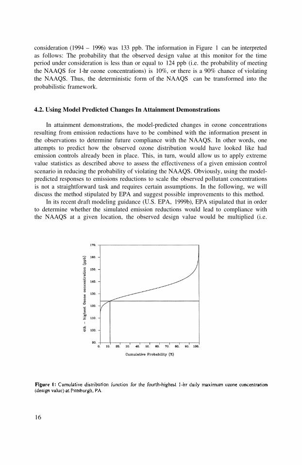
consideration (1994 – 1996) was 133 ppb. The information in Figure 1 can be interpretedas follows: The probability that the observed design value at this monitor for the timeperiod under consideration is less than or equal to 124 ppb (i.e. the probability of meetingthe NAAQS for 1-hr ozone concentrations) is 10%, or there is a 90% chance of violatingthe NAAQS. Thus, the deterministic form of the NAAQS can be transformed into theprobabilistic framework.
4.2. Using Model Predicted Changes In Attainment Demonstrations
In attainment demonstrations, the model-predicted changes in ozone concentrationsresulting from emission reductions have to be combined with the information present inthe observations to determine future compliance with the NAAQS. In other words, oneattempts to predict how the observed ozone distribution would have looked like hademission controls already been in place. This, in turn, would allow us to apply extremevalue statistics as described above to assess the effectiveness of a given emission controlscenario in reducing the probability of violating the NAAQS. Obviously, using the model-predicted responses to emissions reductions to scale the observed pollutant concentrationsis not a straightforward task and requires certain assumptions. In the following, we willdiscuss the method stipulated by EPA and suggest possible improvements to this method.
In its recent draft modeling guidance (U.S. EPA, 1999b), EPA stipulated that in orderto determine whether the simulated emission reductions would lead to compliance withthe NAAQS at a given location, the observed design value would be multiplied (i.e.
16

scaled) by a site-specific Relative Reduction Factor (RRF). EPA defined the relativereduction factor (RRF) as the ratio of the mean model-predicted daily ozone maxima forthe emission control and base cases over all simulated days (U.S. EPA, 1999b). Days withdaily maximum 8-hr average ozone concentrations less than 70 ppb would be excludedfrom the computation of the RRF. The attainment demonstration procedure assumes thatthe distribution of daily maxima for each site will flatten after controls are implemented(e.g., the difference between the 90th percentile concentration and the medianconcentration diminishes once controls are in place), but that a day’s ranking in the tail ofa pre-control distribution is similar to its ranking in the post-control distribution (U.S.EPA, 1999b). The assumption is that lower concentrations which are close to backgroundlevels already are unlikely to be greatly affected by control measures (Lefohn, et al.,1998). This assumption is consistent with the above-mentioned practice of excluding dayswith daily maximum 8-hr average ozone concentrations less than 70 ppb from thecomputation of the RRF.
However, when focussing only on the effect of emission reductions on the upper tailof the predicted distribution by selecting only high ozone days for calculating the RRF,one does not make use of the entire information about the effect of emission reductionspresent in the model predictions. Using the spectral decomposition technique detailed inHogrefe et al. (2000), we calculated the effect of the emission reductions of the 2007 SIPcall on the predicted model distributions for the intra-day, diurnal, synoptic, and baselinetime scales. For example, controls on the ground-level emissions can be expected tolargely affect the diurnal scale while controls on elevated point source would influencelargely the synoptic scale forcings.
The standard deviations for the control and base case simulations as well as theirratio for all components along with the means and their difference for the baselinecomponent in both simulations are presented in Table 1. This calculation was performedfor AIRS station 420031005 near Pittsburgh, PA. These results illustrate that – by makinguse of all 2136 hours of model predictions and disseminating them using the spectraldecomposition technique – additional information can be gained about the model-predicted effect of emission reductions on ozone air quality. In this case, it is evident thatthe spread of the distributions changes most significantly for the synoptic and baselinetime scales, to a lesser degree for the diurnal component, while no change of thedistribution width is predicted for the intra-day component. This suggests that – at least atthis location – the simulated emission reduction scenario that focusses on reducingemissions from elevated point sources is likely to reduce the magnitude of high ozoneconcentrations occurring over extended periods of time (i.e. longer time scales areaffected mostly).
While the model prediction of this effect of emission reductions cannot be readilyevaluated against observations, analysis of long-year records of ozone concentrations alsoshow that the long-term behavior of ozone is different on different time scales. Forexample, Chan et al. (1999) found that the magnitude of the observed intra-dayfluctuations are nearly invariant in time (i.e., no trend), while changes in the magnitude offluctuations on other time scales contributed to an overall downward trend in ozoneconcentrations over Los Angeles. In other words, analyses of observations support thenotion that the effect of emission reductions on model predicted ozone concentrations
17

should be analyzed in terms of the predicted changes in the distributions of differenttemporal components.
To integrate the predicted changes in ozone component distributions into theobserved concentrations for attainment demonstration purposes, we propose the followingmethod: spectrally decompose the hourly ozone time series at a given monitor location,then multiply each hourly component time series by the ratio of control case to base casemodel-predicted standard deviation for the component. Since the baseline component hasa non-zero mean, the mean is subtracted before scaling it in this manner and then addedback after the scaling. In addition, the model-predicted reduction in the mean baselinevalues is subtracted from all observed hourly baseline values. The scaled component timeseries are then added back together; the scaled observed time series is obtained by takingthe exponent of this sum so that the daily maxima can be determined in the ppb scale.Subsequently, extreme value statistics can be applied to determine the effect of thesimulated emission reductions on the exceedance probability. While this scaling approachis somewhat arbitrary, it takes into account the apparent time-scale-specificity of emission
18

reductions. Future research should be directed at quantifying the direct effect of theemission control programs that have been implemented on different spectral componentsof the ozone observations.
To compare the two scaling approaches (i.e., EPA’s and the method proposed here),the CDF for the 1-hr design value is re-calculated after all observations are scaled by boththe RRF method and the component adjustment method. For the RRF approach, weassume that all observed values in the tail of the observed distribution (which are used tocomputed the CDF of the design value) are uniformly reduced by the RRF. Figure 2depicts these design-value CDF’s for the Pittsburgh, PA monitor using the 2007 SIP callemission reduction scenario (U.S. EPA, 1998a) relative to the 1995 base case, asdescribed in section 2. From Figure 2, it can be seen that both methods yield differentCDF’s. At this location, the RRF scaling method predicts that the 2007 NOx SIP callemission reductions would reduce the probability of violating the 1-hr NAAQS from 90%to 15%, while the component adjustment approach predicts that the probability ofviolating the NAAQS is near 0%. In other words, whereas the EPA-suggested method stillshows a 15% probability of violating the NAAQS, the component adjustment methodsuggests compliance with the ozone NAAQS at this location with emission reductionsproposed in the SIP call.
5. SUMMARY
Building upon a recent study by Hogrefe and Rao (2001), we presented an integratedobservational-modeling approach to transform the deterministic nature of attainmentdemonstrations for the NAAQS for 1-hr and 8-hr ozone concentrations into theprobabilistic framework. The application of extreme value statistics in estimating theprobability of exceeding the NAAQS has been illustrated. The proposed probabilisticframework would enable decision makers to assess their chances of success in meeting thestandard when control measures aimed at attaining the NAAQS are implemented. Thispaper introduced a method to account for the time-scale specificity of the effects ofemission reductions when scaling the observations. Extended modeling periods ratherthan episodic simulations are needed for model evaluation as well as to assess the effectof emission reductions on different time scales.
6. ACKNOWLEDGMENTS
7. REFERENCES
This work is supported by New York State Energy Research and DevelopmentAuthority under contract No. 6085.
Biswas, J., and S. T. Rao, 2001: Uncertainties in Episodic Ozone Modeling Stemming from Uncertainties inMeteorological Fields; J. Appl. Meteor., 40, 117 – 136.
Biswas, J., S. T. Rao, C. Hogrefe, C. W. Hao, and G. Sistla, 2001: Evaluating the Performance of Regional-Scale Photochemical Modeling Systems: Part III – Ozone Precursor Predictions; Atmos. Environ.; in press
19

Breiman, L., and C. J. Stone, 1985: Broad Spectrum Estimates and Confidence Intervals for Tail Quantiles;Technical Report No. 46; Department of Statistics, University of California, Berkeley, CA.
Chan, D., S. T. Rao, I. G. Zurbenko, and P. S. Porter, 1999: Linking Changes in Ozone to Changes inEmissions and Meteorology; Proceedings of the Air Pollution ’99 Conference, Wessex Institute ofTechnology, WIT Press, Wessex, U.K., 664 – 675.
David, H. A., 1981: Order Statistics; John Wiley: New York, pp 8 – 22.Efron, B., 1979: Computers and the Theory of Statistics: Thinking the Unthinkable; SIAM Rev.; 21 (4).Gumbel, E .J., 1958: Statistics of Extremes; Columbia University Press: New York; pp 75 – 155.Hogrefe, C., S. T. Rao , I. G. Zurbenko, and P. S. Porter, 2000: Interpreting the Information in Ozone
Observations And Model Predictions Relevant to Regulatory Policies in the Eastern United States; Bull.Amer. Meteor. Soc., 81, 2083 - 2106.
Hogrefe, C., S. T. Rao, P. Kasibhatla, G. Kallos, C. J. Tremback, W. Hao, D. Olerud, A. Xiu, J. McHenry, J.,and K. Alapaty, 200la: Evaluating the Performance of Regional-Scale Photochemical Modeling Systems:Part I - Meteorological Predictions; Atmos. Environ., 35, 4159 - 4174.
Hogrefe, C., S. T. Rao, P. Kasibhatla, W. Hao, G. Sistla, R. Mathur, and J. McHenry, 2001b: Evaluating thePerformance of Regional-Scale Photochemical Modeling Systems: Part II - Ozone Predictions; Atmos.Environ., 4175-4188.
Hogrefe, C., and S. T. Rao, 2001: Demonstrating Attainment of the Air Quality Standards: Integration ofObservations and Model Predictions into the Probabilistic Framework; J. Air Waste Manag. Assoc., 51,1060–1072.
Lefohn, A. S., D. S. Shadwick, and S. D. Ziman, 1998: The Difficult Challenge of Attaining EPA’s New OzoneStandard, Environ. Sc. Tech., Pol. Anal., 32, 276a- 282a.
Porter, P. S., S. T. Rao, I. G. Zurbenko, A. M Dunker, and G. T. Wolff, 2001: Ozone Air Quality over NorthAmerica: Part II – An Analysis of Trend Detection and Attribution Techniques; J. Air Waste Manag.Assoc., 51, 283 – 306.
Rao, S. T., G. Sistla, V. Pagnotti, W. B. Petersen, J. S. Irwin, and D. B. Turner, 1985: Resampling andExtreme Value Statistics in Air Quality Model Performance Evaluation; Atmos. Env., 19, 1503-1518.
Rao, S. T. and G. Sistla, 1992: On the Use of Numerical Models in Ozone Attainment Demonstrations; In Airpollution modeling and its applications IX; Dop, H.v., Kallos, G., Ed.; Plenum Press: New York, NY, 41 -48.
Rao, S. T., and I. G. Zurbenko: Detecting and Tracking Changes in Ozone Air Quality; J. Air Waste Manag.Assoc., 44, 1089 – 1092.
Rao, S. T., I. G. Zurbenko, R. Neagu, P. S. Porter, J.Y. Ku, and R. F. Henry, 1997: Space and Time Scales inAmbient Ozone Data; Bull. Amer. Meteor. Cos., 78, 2153 – 2166.
Rao, S. T., C. Hogrefe, J. Biswas, H. Mao, I. G. Zurbenko, P. S. Porter, P. Kasibhatla, and D. A. Hansen, 2001:How Should the Photochemical Modeling Systems be used in Guiding Emissions ManagementDecisions?, Air Pollution Modeling And Its Applications XIV, Gryning, S. E. and F. Schiermeier, Eds.,Kluwer Academic / Plenum: New York, 25 – 34.
Roberts, E. M., 1979: Review of Statistics of Extreme Values with Applications to Air Quality Data Part I.Review; J. Air Poll. Cont. Assoc., 29, 632.
U.S. Environmental Protection Agency, 1998a: National Air Pollutant Emission Trends Update, 1970-1997;EPA-454/E-98- 007, U.S. Environmental Protection Agency, Research Triangle Park, NC 27711, 1998.Available online at http://www.epa.gov/ttn/chief/trends/ trends97
U.S. Environmental Protection Agency, 1998b: Finding of Significant Contribution and Rulemaking forCertain States in the Ozone Transport Assessment Group Region for Purposes of Reducing RegionalTransport of Ozone; Federal Register, October 27, 1998, Vol. 63, No. 207, pp. 57355-57404. Availableonline at wais.access.gpo.gov
U.S. Environmental Protection Agency, 1999a: Procedures for Developing Base Year and Future Year Massand Modeling Inventories for the Tier 2 Final Rulemaking; EPA420-R-99-034, U.S. EnvironmentalProtection Agency, Research Triangle Park, NC 27711. Available online athttp://www.epa.gov/orcdizux/regs/ld-hwy/tier-2/frm/tsd/r99034.pdf
U.S. Environmental Protection Agency, 1999b: Draft Report on the Use of Models and Other Analyses inAttainment Demonstrations for the 8-Hour Ozone NAAQS; EPA-44/R-99-0004; United StatesEnvironmental Protection Agency, Research Triangle Park, NC 27711.
U.S. Envirionmental Protection Agency, 2000: Regional Modeling Center Homepage. Available online athttp://www.epa.gov/ttn/ scram/regmodcenter/t28.htm
20

DISCUSSION
Why do you think that the parameters “a” and “b” in theexponential distribution are the same for each of three years ?What is the dispersion of your estimates of the fourth highestvalue ?
Ch. HOGREFE To answer the first part of your question, the parameters “a” and“b” are estimated from the total distribution consisting of all 3years of observations, not for the individual years. When different3-year periods are considered, the parameters “a” and “b” change,and as a result the calculated CDF of the highest concentrationalso changes. In other words, the inter-annual variability presentin the observations is not accounted for in the methodology. Thisis due to the definition of the NAAQS which focusses on a single3-year period for the attainment demonstration process. Thedispersion of the estimates of the fourth highest value isintroduced by both interannual variability if other 3-year periodsare considered, as well as by model-to-model differences inpredicted RRF. In our experience, the former is greater than thelatter.
A comment. We cannot change the rules laid down by the USEPA, but this paper shows that the application of the ozone rulesis very difficult. Alternative rules could produce equivalentbenefits for air quality, but would be easier to assess ?
I agree. The present NAAQS rules are very difficult to addresswith the current air quality modeling tools. The presentedapproach attempts to bridge this gap, but clearly future efforts arenecessary, and a change in the way the NAAQS are defined mightlead to a more consistent attainment demonstration process.
B. FISHER
Ch. HOGREFE
E. GENIKHOVITCH
21

This page intentionally left blank

INTEGRATED REGIONAL MODELLING
Chairpersons: D. AnfossiA. BaklanovP. Builtjes
Rapporteurs: J. BrechlerB. CarissimoC. MensinkE. Renner

This page intentionally left blank

CHANGING ATMOSPHERIC ENVIRONMENT,CHANGING VIEWS - AND AN
AIR QUALITY MODEL‘S RESPONSEON THE REGIONAL SCALE
Adolf Ebel1
ABSTRACTExperiences having resulted from the development and application of a specific airquality modelling system (EURAD) are discussed. Reasons for complex modellingand motivations evolving from a quickly growing field of atmospheric science arepresented. It is argued that meteorology and atmospheric chemistry form an in-tegral interdependent system of processes requiring an integral approach to theirnumerical modelling. A few examples of the application of a regional air pollutionmodel to a broader set of environmental topics including the tropopause region aregiven. Aerosol simulation, chemical data assimilation and intensification of opera-tional ozone forecast are viewed as important and challenging tasks for air qualitymodelling in the near future.
1. INTRODUCTION
The aim of this paper is not so much to discuss the development of air qualitymodels than to demonstrate the change of the approach to the tasks and goals ofchemical transport simulations by air quality modellers. Of course, there exists anintimate interdependence of intelligent definition of modelling goals and smart mo-del improvement. Yet it may well be debated which really will be the driving forceof progress in the field of air pollution modelling in the future: the improvement ofthe tool, i.e. the model, or the growing skill of controlling the modelling process bythe users of the tool, for instance, by putting stronger efforts on the evaluation ofnumerical simulations. This aspect has clearly and convincingly been emphasized bya critical review of meso-scale air pollution modelling by Russel and Dennis (2000).
1 Adolf Ebel, EURAD Project, University of Cologne, Institute for Geophysics and Meteoro-logy, and Rhenish Institute for Environmental Research, Aachener Str. 201–209, 50931 Cologne,Germany; [email protected]
Air Pollution Modeling and Its Application XV, Edited byBorrego and Schayes, Kluwer Academic/Plenum Publishers, New York, 2002 25

The study is based on experiences gained with a specific regional air quali-ty model, namely the EURAD system (European Air Pollution Dispersion model:Hass et al., 1993, Ebel et al., 1997) which the author is most familiar with. It isnot intended to dwell on the characterization and comparison of different modelsor modules. There are various publications to which the interested reader may refer(e.g. Russel and Dennis, 2000; Ebel, 2000; Dodge, 2000). Nevertheless, it is hopedthat conclusions about changing models and alterations of the modelling processduring the last one or two decades also reflect experiences of other modellers withother models and thus can be generalized to a certain degree.
The EURAD modelling project was started when emission of sulfur and acidi-fication were still an issue of highest priority for environmental policy. Therefore,a chemistry transport model focusing on acidic components in the atmosphere waschosen as the core model of the EURAD system. It was the Regional Acid Deposi-tion Model (RADM; Chang et al., 1987, improved chemical mechanism RACM byStockwell et al., 1990) which was adjusted to European conditions and has graduallybeen transformed to the so–called EURAD–CTM (EURAD Chemistry TransportModel) and further extended to more comprehensive versions (e.g. CTM2, Hass1991). Yet due to successful reduction of sulfur emission, a dramatic increase inphoto-oxidant levels during summer smog episodes and the public awareness of thischange of air quality problems the focus of the model and simulations soon hadto move from to A similar modelling strategy as adopted by EURAD forthe larger meso–scale was followed by the so–called TADAP project with ADOM(Venkatram et al., 1988) as the core model. There were attempts to organize closercooperation between these and other regional model activities in the frameworkof the first European environmental research project EUROTRAC. Unfortunate-ly, their success was rather limited. Yet for the EURAD project strongly involvedin EUROTRAC it has to be emphasized that the challenges resulting from thisinvolvement were extremely fruitful for the development of its model system. Onthe smaller meso–scale an approach similar to that of EURAD was chosen for theKAMM/DRAIS air pollution model system (Nester et al., 1995). The regional mo-delling initiative in EUROTRAC was successful with initiating and intensifyingemission research and modelling for advanced numerical simulations on a Europeanscale (Friedrich, 1997). It also paved the way for cooperative air quality modellingon local and urban scales in the framework of EUROTRAC (Moussiopoulos, 1995).
2. DESIGN OF MODEL AND MODELLING CONCEPT
The EURAD system consists of three models treating chemistry and transport(EURAD-CTM), meteorology (MM5, Grell et al., 1994) and emissions (EURADEmission Model, EEM; Memmesheimer et al., 1991). It is an Eulerian multilayergridpoint model system for meso-scale applications. Depending on the problem che-mistry and meteorology can be integrated simultaneously or sequentially. The usualmode of application is off-line calculation of chemistry and transport. The horizontalextension depends on the horizontal resolution wanted (European scale,
26

about 50 km; local scale, not less than 1 km). Sequential nesting is possible andnow used in most applications. 100 hPa is usually chosen as the upper boundary. Ithas been extended to 10 hPa for simulations including the tropopause region. Moredetailed descriptions of the model can be found elsewhere (e.g. Hass et al., 1993;Jakobs et al., 1995). In the context of this paper it is more interesting and adequateto review some basic considerations governing the model design.
The basic philosophy of the design of the EURAD system was that it shouldbe an as complete as possible numerical representation of the environmental systemon a regional scale. The EURAD project followed the idea of Earth system analysis(Schellnhuber and Wenzel, 1998) for its atmospheric compartment before this termwas coined by modern geoscience. As a consequence one had to go to complexityinstead of simplicity. From the scientific view it is clear that the neglect or simpli-fication of processes in the simulation of a non–linear system like the atmosphericenvironment is always dangerous. From the view of computational science it is ob-vious that computer and software performance will still considerably grow in thefuture. Therefore, it would be inexcusable not to aim at an as complete and relia-ble as possible virtual realization of the atmospheric environmental system throughexploitation of fast growing computational power.
The integral view of the atmospheric environment of the EURAD project requi-red to put equal weight on the analysis arid development of the chemical transportand meteorological models. So the aim was not to built new models but to designan interactive dynamical and chemical system with the help of leading experts fromboth fields. (Looking back there was great excitement in this collaboration. AndI want to acknowledge enthusiastically that EURAD considerably gained from fri-endly help and critical perturbations provided by many colleagues.)
Two decades ago it was not very common (though not completely new) to treatchemical and dynamical simulations with the same weight in the same project. Se-veral CTMs followed the idea that one could treat meteorology simply as an inputproblem. Yet employing meteorological forecast models to generate this input, itdid not last long to recognise that a model with perfect pressure pattern predicti-ons would not necessarily provide good transport parameters. There were (and stillare) problems with turbulence, clouds precipitation etc. On the other hand, trans-port parameterizations and calucations in CTMs, e.g. bounday layer effects, couldgain a lot from advanced meteorological schemes. Furthermore, the combination ofdynamical, chemical and also emission modelling provided a much higher degreeof flexibility for scientific studies and practical applications. Studies of the impactof climate change and geographical conditions (particularly complex terrain) or ofdifferent levels of the troposphere up to the lower stratosphere (Ebel et al., 1991)became easier to design. And the range of essential sensitivity studies, for instance,about effects of clouds, fog, aerosols, biogenic emissions or land use changes, couldadvantageously be expanded. From the view of the integral treament of the atmo-sphere it was clear from the beginning on that not only global, but also regionalmodelling had to deal with aerosols, now being a high priority issue of environmen-tal resarch after science has progressed and our views have changed. Yet there wasa time when experimental capacities and interests were nearly totally absorbed by
27

photo–oxidants in regional air quality research such emphasis made it difficult, butnot impossible, to find support for the development of modules adequately dealingwith particulates in atmospheric and environmental models. Watching weather fo-recast and its improvement through data assimilation it was easy to conclude at avery early state of air quality modelling that it would also considerably profit fromthis method in future. The broad (though not yet general) acknowledgement of thisconcept as a useful feasable improvement of chemical transport simulation neededeven more time than the aerosol case.
It is interesting to see that the former disadvantage of long integration timesof complex models regarding their practical application to long-term assessmentstudies or operational air quality forecasts is gradually overcome by increasing com-puter performance (Jakobs et al., 2001).
The following sections are illustrating the above remarks with selected examp-les of EURAD system applications. The reader will note that EURAD always wasa child of its time but sometimes a little bit special in choosing its playground.
3. EXPLORATION OF PROCESSES
The evaluation of the role of processes controlling the distribution of trace sub-stances in the atmosphere is essential for scientific as well as practical reasons. Inboth cases they are needed to increase our understanding of cause–effect relation-ships and to find priorities, i.e. develop strategies, for optimal model development aswell as environmental management. Process studies can be carried out in differentways. One of the most efficient methods is sensitivity analysis. Another one whichrequires larger efforts is process-oriented evaluation. Three examples of analysesconcerned with the role of particular processes are addressed in this section.
Firstly, an aspect difficult to deal with but most fascinating for exploring theatmospheric chemistry–transport system is the interaction of processes, particularlywith respect to possible non–linearities. Sensitivity studies of the impact of climatechange on future air quality are, therefore, an interesting case of model application.For instance, climate trend will cause land type changes (e.g. a possible increase ofdesertification in Spain) and thus changes of boundary layer behaviour and biogenicemissions. Both will influence atmospheric chemistry. Yet land type changes mayalso be exptected as a direct consequence of population growth. Furthermore, onecan think of scenarios where these direct changes have a larger regional effect onatmospheric composition than those indirectly induced by climate change makingthe analysis of climate trend effects by only observing air quality trends an impos-sible task. Models are needed to unravel multiple causes of identical effects.
Another illuminating example is the decisive role which subsidence of ozonecontaining air from the free troposphere plays for the ozone budget of the atmos-pheric boundary layer (ABL) during photo-smog episodes (Memmesheimer et al.,1997). It may be as efficient as chemical production regarding the contribution toaccumulation of ozone in polluted regions. And chemistry appears to react on suchinflux becoming less productive with increasing ozone flux convergence. For the first
28

time this could be shown for a summer smog episode in Central Europe in 1990.The model results also show that vertical transport of ozone through convectionduring photo-smog episodes into the free troposphere is not very effective since itis counteracted by subsidence. Only at the end of such episodes caused by frontalsystems boundary layer ozone can be mixed into upper layers in larger quantities.Of course, substances like having no sources at higher levels will experience asignificant loss in the ABL due to vertical mixing and advection under the sameconditions when the ozone budget is growing through this process.
Atmospheric aerosol offers a third example of possible process interactions. Itscomplex role for air quemistry and transport is not yet completely understood. Yetregarding air pollution simulations, there have been early suspicions and hints ofits relevance though they were ignored or set very low priority for quite a while inEuropean regional air quality research. Implementing a simple mechanism for secon-dary anorganic aerosol formation in EURAD (Kötz, 1991) it became evident thatlong-range transport and deposition of nitrogen compounds could more realisticallybe simulated in several cases (Ackermann et al., 1995). More comprehensive modelstudies of aerosol formation, transport and effects are needed and going on with theaim to support applied air quality analyses and programmes. In this respect, modeldevelopment is following practical needs to a great extent.
4. EXPLORATION OF EPISODES AND SEQUENTIAL NESTING
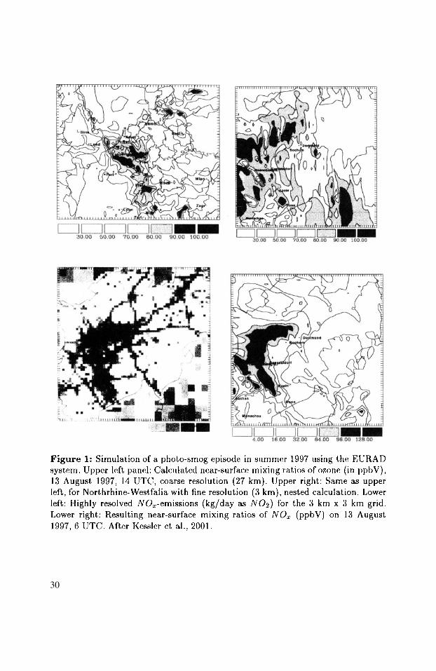
One of the first cases in which the EURAD project became involved was theaccident of the nuclear power plant in Chernobyl. Other episodes were focusing onperiods and areas which were of special interest to environmental agencies in theframework of assessment studies. The selection of quite a large number of caseswas motivated by the involvement in ongoing field experiment or availability ofparticular atmospheric data for model evaluation. First applications were mainlyconcerned with the problem of long-range transport of pollutants of different kindin Europe. Small meso–scale aspects were delt with in collaboration with other at-mospheric modellers and models (Borrego et al., 1995; Moussiopoulos, 1995; Nesteret al., 1995). Yet the recognition of strong coupling of scales, the demand for higherresolution studies motivated by environmental assessment and a growing numberof small meso–scale and local field experiments (e.g. TRACT: Fiedler and Borrell,2000; BERLIOZ: Corsmeier et al., 2001), the need for consistent boundary con-ditions for urban and local models and the availability of growing computationalpower finally lead to the installation of a sequential nesting option in EURAD (Ja-kobs et al., 1995). The increase of information through application of this methodis illustrated in Fig. 1 derived from a simulation of a photo-smog episode in Au-gust 1993 in Central Europe (Kessler et al., 2001). Using sequential nesting theresolution is increased from 27 km (Central Europe and UK) to 3 km (State ofNorthrhine-Westfalia). The growth of information about the spatial distributionof pollutants with increasing resolution is obvious. It is also evident from themap of emissions that the price one has to pay is more detailed input data.
29
30
This is still a fundamental obstacle to efficient refinement of the simulations. Procee-ding to still smaller scales requires explicit calculations of meteorological processeswhich are parameterized for calculations with coarser resolution. To achieve thisEURAD has been expanded by inclusion of a high resolution meteorological driverfor local applications (CARLOS system, Brücher et al. 2000, Kessler et al., 2001).
5. EXPLORATION OF ATMOSPHERIC COMPARTMENTS
Feeling committed to an integral view of the atmosphere the application ofEURAD has been expanded beyond its main focus, namely the polluted ABL. Themodular and multi-layer design of the parent models of EURAD, i.e. RADM andMM5, provided an excellent basis for this aspect of research and application. Theconviction was that an advanced tool of computational science like EURAD hadto be tried out on less safe grounds where little or no guiding laboratory or fieldexperiments have been available (e.g. near the tropopause) or where the validity ofcertain model assumptions still had to be tested (e.g. over mountainous terrain).Therefore, the whole system or parts of it were used to look into problems likethe Kuwait oil fires during the Gulf war, regional effects of layered and convectiveclouds in the free troposphere or the behaviour of transport and chemistry in thetropopause region. Two examples are briefly mentioned in this section.
An exciting and quite successful application of the EURAD system was thestudy of tracer transport over Alpine regions (Seibert et al.). One of the major pro-blems under such extreme conditions is the handling of ABL and free troposphereinteractions in the dynamic as well as chemical part of the system. Again, coope-ration with experimentalists and data analysts was essential for the generation ofsufficiently reliable model results.
The EURAD system provided the first successful meso-scale simulation of astratospheric intrusion of ozone occuring over Europe (Ebel et al., 1991). The modelto handle chemical transport processes in the tropopause region the model was rede-signed for the treatment of the upper troposphere and lower stratosphere. RADM2has been adjusted to the conditions of the tropopause region by inclusion of typicalstratospheric gasphase and heterogeneous reactions essential at those heights. Theresult is CHEST2, a CHEmistry model for the lower Stratosphere and Troposphere,version 2 (Hendricks et al., 1999; 2000). This model version was intensively used ina project on air traffic emissions (Schumann et al., 1997) for the assessment of theregional impact of air traffic on the ozone budget around the tropopause focusingon the Northatlantic flight corridor, also taking into accout the impact of intrusionsof stratospheric air into the troposphere. A series of numerical studies was carriedout to explore the efficiency of stratosphere–tropsphere exchange at northern midd-le latitudes and to quantify its contribution to the tropospheric ozone budget inparticular (Kowol–Santen et al., 2000; Ebel et al., 1996).
31

6. EXPLORATION OF VALIDITY, RELIABILITY AND FUTURE:CONCLUDING REMARKS
Expanding the range of application causes a problem of model evaluation. Inthe case of the EURAD system considerable efforts have been made to find out thevalidity of simulation results where it was possible. Yet it is obvious that a generalconfirmation of model validity and, therefore, reliability is difficult to achieve (Ebelet al., 2000). As a consequence, the efforts of model evaluation by comparison withreal world data and also model intercomparison still have to be intensified.
Even though the increase of model complexity through addition of new physicsand chemistry may cause a problem of general accuracy on short terms this way isnecessary to bring CTMs closer to reality. This is clearly evident for the simulationof atmospheric aerosols and their effects, particularly, when its organic fraction istaken into account (Schell et al., 2001).
Future promising directions of model development and application for CTMs ingeneral and EURAD in particular are their perfection with respect to the treatmentof aerosols (being a consequence of the changing view of the relevance of particulatematter in the atmosphere), the exploitation of data assimilation methods (Elbernand Schmidt, 2001; being more and more recognised as a feasable and rewardingtechnique for CTMs, too) and operational air pollution forecasts which are becomingmore frequent at present.
7. ACKNOWLEDGEMENTS
The author is greatly indebted to M. Memmesheimer, H.J. Jakobs, H. Elbern,H. Feldmann, G. Piekorz, Ch. Kessler and E. Friese from the Rhenish Institute forEnvironmental Research at the University of Cologne for kind support of this paper.He gratefully acknowledges fruitful discussions with M. Kerschgens, W. Brücherand H. Kunz. Projects on which this study is based were financially supported bythe Ministries of Research of the FRG and the State NRW (BMBF, MWF), theUmweltbundesamt (UBA), Berlin, and the Environmental Agency of NRW (LUA).Data have been provided by the University of Stuttgart (IER), EMEP, UBA andLUA (emissions) and the ECMWF (meteorology) via the German Weather Service(DWD).
8. REFERENCES
Ackermann, I.J., Hass, H., Memmesheimer, M., Ziegenbein, C. , Ebel, A., 1995, Theparameterization of the sulfate–nitrate–ammonia aerosol system in the long–rangetransport model EURAD, Meteor. Atmos. Phys. 57, 101–114.
Borrego, C., Coutinho, M., Barros, N., 1995, Intercomparison of two meso–meteorologicalmodels applied to the Lisbon region, Meteor. Atmos. Phys. 57, 21–29.
Brücher, W., Kessler, Ch., Kerschgens, M., Ebel, A., 2000, Simulation of traffic inducedair pollution on regional to local scale, Atmos. Environm. 27, 4675–4681.
Chang, J.S., Brost, R.A., Isaksen, I.S.A., Madronich, S., Middleton, P., Stockwell, W.R.,Walcek, C.J., 1987, A three–dimensional Eulerian acid deposition model: physical
32

concepts and formulation, J. Geophys. Res. 92, 14681–14700.Corsmeier, U., Kalthoff, N., Vogel, B., Hammer, M.-U., Fiedler, F., Kottmeier, Ch.,
Volz-Thomas, A., Konrad, S., Glaser, K., Neininger, B., Lehning, M., Jaeschke, W.,Memmesheimer, M., Rappenglück, B., Jakobi, G., 2001, Ozone and PAN formationinside and outside of the Berlin plume – process analysis and numerical processsimulation, J. Atmos. Chem., in press.
Dodge, M.C., 2000, Chemical oxidant mechanisms for air quality modelling: critical re-view, Atmos. Environm. 34, 2103–2130.
Ebel, A., 2000, Chemical transfer and transport modelling, in: Transport and ChemicalTransformation of Pollutants in the Troposphere, P. and P.M. Borrell, eds., Springer,Vol. 1, p. 85–128.
Ebel, A., Hass, H., Jakobs, H.J., Laube, M., Memmesheimer, M., Oberreuter, A., Geiß,H., Kuo, Y.-H., 1991, Simulation of ozone intrusion caused by a tropopause fold andcut–off low, Atmos. Environm., 25A, 2131 – 2144.
Ebel, A., Elbern, H., Hendricks, J., Meyer, R., 1996, Stratosphere–troposphere exchangeand its impact on the structure of the lower stratosphere, J. Geomag. Geoelectr., 48,135–144.
Ebel, A., Elbern, H., Hass, H., Jakobs, H.J., Memmesheimer, M., Laube, M., Oberreuter,A., Piekorz, G., 1997, Simulation of chemical transformation and transport of airpollutants with the model system EURAD, in: Transport and Chemical Transfor-mation of Pollutants in the Troposphere, P. Borrell et al., eds., Vol. 7: TroposphericModelling and Emission Estimation, A. Ebel, R. Friedrich, H. Rodhe, eds., SpringerVerlag, p. 27–45.
Ebel, A., Memmesheimer, M., Jakobs, H.J., Kessler, Ch., Piekorz, G., Feldmann, H.,2000, Reliability and validity of regional air pollution simulations, in: Air PollutionVIII, J.W.S. Longhurst, C.A. Brebbia and H. Power, eds., WITpress, Southampton,Boston, p. 12-30.
Elbern, H., Schmidt, H., 2001, Ozone episode analysis by four–dimensional variationalchemistry data assimilationr, J. Geophys. Res. 106, 3569–3590.
Friedrich, R., 1997, GENEMIS: Assessment, improvement, and temporal and spatial di-saggregation of European emission data, in: A. Ebel, R. Friedrich, H. Rodhe, eds.,Tropospheric Modelling and Emission Estimation, Springer Verlag, Heidelberg, p.181–214.
Grell, G., Dudhia, J., Staufer, D., 1994, A description of the fifth-generation PennState/NCAR mesoscale model (MM5), Technical Note NCAR/TN-398+STR, Na-tional Center of Atmospheric Research, Boulder, Colorado.
Hass, H, 1991, Description of the EURAD Chemistry-Transport-Model Version 2(CTM2), Mitteilungen aus dem Institut für Geophysik und Meteorologie der Uni-versitat zu Köln, Nr. 83.
Hass, H., Ebel, A., Feldmann, H., Jakobs, H.J., Memmesheimer, M., 1993, Evaluationstudies with a regional chemical transport model (EURAD) using air quality datafrom the EMEP monitoring network, Atmos Environ. 27A, 867–887.
Hendricks, J., Lippert, E., Petry, H., Ebel, A., 1999, Heteorogeneous reactions on and insulfate aerosols: implications for the chemistry of the midlatitude tropopause region,J. Geophys. Res. 104, D5, 5531–5550.
Hendricks, J., Lippert, E., Petry, H., Ebel, A., 2000, Implications of subsonic aircraftNOx emissions for the chemistry of the lowermost stratosphere: Model studies onthe role of bromine, J. Geophys. Res. 105, D5, 6745–6759.
Jakobs, H.J., Feldmann, H., Hass, H., Memmesheimer, M., 1995, The use of nested modelsfor air pollution studies: an application of the EURAD model to a SANA episode.J. Appl. Meteor. 34, 6, 1301–1319.
33
Jakobs, H.J., Tilmes, S., Heidegger, A., Nester, K., Smiatek, G., 2001, Short–term ozoneforecasting with a network model system during Summer 1999, J. Atmos. Chem., inpress.
Kessler, Ch., Brücher, W., Memmesheimer, M., Kerschgens, M., Ebel, A., 2001, Simula-tion of air pollution with nested models in Northrhine-Westfalia, Atmos. Environ.35 Suppl: S3-S12.
Kötz, A., 1991, Bedeutung der Aerosole für den Ferntransport von Schadstoffen in derTroposphäre, Mitteilungen aus dem Institut für Geophysik und Meteorologie der Uni-versität zu Köln, Nr. 81.
Kowol–Santen, J., Elbern, H., Ebel, A., 2000, Estimation of cross–tropopause air massfluxes at midlatitudes: comparison of different numerical methods and meteorologicalsituations, Mon. Weather Rev. 128, 4045–4057.
Memmesheimer, M., Tippke, J., Ebel, A., Hass, H., Jakobs, H.J., Laube, M., 1991, Onthe use of EMEP emission inventories for European scale air pollution modellingwith the EURAD model, in: EMEP workshop on Photooxidant Modelling for Long-Range Transport in Relation to Abatement Strategies, Berlin, 16.–19. April 1991, p.307–324.
Memmesheimer, M., Roemer, M., Ebel, A., 1997, Budget calculations for ozone and itsprecursors: seasonal and episodic features based on model simulations, J. Atmos.Chem. 28, p. 283–317.
Moussiopoulos, N., 1995, The EUMAC Zooming Model, a tool for local-to-regional airquality studies, Meteor. Atmos. Phys. 57, 115-134.
Nester, K., Panitz, H.J., Fiedler, F., 1995, Comparison of the DRAIS and EURAD modelsimulation of air pollution in a mesoscale area, Meteor. Atmos. Phys. 57, 135–158.
Russel, A., Dennis, R., 2000, NARSTO critical review of photochemical models andmodeling, Atmos. Environ. 34, 2283–2324.
Seibert, P., Feldmann, H., Neininger, B., Bäumle, M., Trickl, Th., 2000, South foehn andozone in the Eastern Alps - case study and climatological aspects, Atmos. Environ.34, 1379–1394.
Schell, B., Ackermann, I.J., Hass, H., Binkowski, F.S., Ebel, A., 2001, Modeling theformation of secondary organic aerosol within a comprehensive air quality modelsystem, J. Geophys. Res., in press.
Schellnhuber, H.J., Wenzel, V., eds., 1998, Earth System Analysis, Springer Verlag, Ber-lin, Heidelberg.
Schumann, U., Chlond, A., Ebel, A., Kärcher, B., Pak, H., Schlager, H., Schmitt, A.,Wendling, P. (eds), 1997, Pollutants from Air Traffic – Results of Atmospheric Re-search 1992-1997, Mitteilung 97–04, Deutsches Zentrum für Luft- und Raumfahrte.V.
Stockwell, W.R., Kirchern, F., Kuhn, M., 1997, A new mechanism for regional atmos-pheric chemistry modelling, J. Geophys. Res. 102, D22, 25847–25879.
Venkatram, A., Karamanchandani, P.K., Misra, P.K., 1988, Testing a comprehensive aciddeposition model, Atmos. Environ. 22, 737–747.
34
DISCUSSION
A. HANSEN As an example of how increasing the complexity of a model candegrade its performance (as measured by point to grid cellcomparisons) is the inclusion of clouds. Meteorological modelscannot simulate precisely in time and space cloud fields such thatactinic fluxes, soil moisture, temperature, etc. are not preciselysimulated, although in a statistical sense the model may beperforming adequately. How do you deal with this issue ?
A. EBEL Obviously, the question is touching a rather crucial point of airquality modelling. Various attempts have been made with the aim toimprove the model system (EURAD) with respect to performance ofcloud and precipitation simulation (exploring, e. g., differentparameterizations), but general solutions seem to be far away. It isemphasized that similar problems are encountered in cloud-freephoto-oxidant simulations when local changes are controlled bysubgrid processes to be parametrized in models. Various methodshave been employed to cope with such problems of representativityand uncertainties of estimates of subgrid effects. These aresensitivity studies, model comparisons, adjustment of resolution(nesting) and evaluation studies in cases where suitable data havebeen available. It has also proven helpful to provide estimates of therange of reliability of simulated data.
T. HALENKA In context of the models complexity and their “perfection”, couldyou estimate the impact of uncertainty in emission on the results ofthe modelling ?
A. EBEL A large number of studies regarding the role of accuracy of emissionestimates for the performance of air quality models can be found inthe literature. The results differ in dependence of the scenariosinvestigated and vary with the chemical species used to evaluate thesensitivity of models to emission uncertainties. For instance, acomprehensive study employing the EURAD model system wasrecently conducted by B. Wickert (Berechnung anthropogenerEmissionen in Deutschland fuer Ozonsimulationen;Modellentwicklung und Sensitivitaetsstudien, Thesis, University ofStuttgart, 2001). The analysis is focusing on ozone formation underconditions of NOx limitation. Such situation is characterized byhigher sensitivity to NOx then to NMVOC emission changes.Differences up to 10% were found for spatially averaged ozone
35

mixing ratios in case of rather strong (and - in special cases -possible) deviations of emissions from a reference scenario.
G. SCHAYES Data assimilation is important for short term modelling. Theimprovement degrades rapidly with time. The technique is thususeful for applied models. Is it also important for research models ?
A. EBEL Formulation of improved initialization fields for chemical transportmodels is only one aspect of the application of data assimilationmethods to air chemistry simulations. The degradation of the initialimprovement with time (say, after 24 hours) can be overcome to acertain degree if one succeeds to implement parameters whose futuredevelopment is known and which exert sufficient control on thesimulated chemical species. Using the EURAD system it could beshown that anthropogenic and natural emissions fulfil this condition.Data assimilation is also a promising method to be used for research.In the case of air chemistry it can well be applied to the design ofimproved and consistent fields of reactive species, to the evaluationof reaction coefficients, to the design of observing systems and theevaluation of models. Refer to H. Elbern and H. Schmidt, 4D-vardata assimilation and its numerical implications for case studyanalysis, accepted for publication in: IMA Series “Mathematics andIts Applications, Reactive Flow and Transport Phenomena”, issue on“Atmospheric Modeling”, Minneapolis, Minnesota, 2002.
36

DEVELOPMENT OF A REGIONAL MODEL FOROZONE FORECASTING AND
ACIDIC DEPOSITION MAPPING
Al Tang, Neville Reid, P.K. Misra1
1. INTRODUCTION
Simulation of atmospheric ozone and acid deposition has been done since the 1980’susing comprehensive 3-D models, such as the Acid Deposition and Oxidant Model(ADOM), the Regional Acid Deposition Model (RADM), etc. These models includechemistry modules consisting of large numbers of chemical species and reactions, thuscreating large uncertainties and computing overhead in their applications. Foroperational application of models, however, it is desirable to develop and use modelswhich have reasonable skills in reproducing the observations, and yet do not require largecomputing overhead.
The Ontario Ministry of Environment has a need for operational application ofphoto-chemical and acid deposition models to forecast ozone levels in the atmosphereand produce acid deposition maps. Toward that end a model has been developed usingthe ADOM model, with the chemistry module replaced by the Graham Johnson scheme.This reduces uncertainties and computing time significantly, enabling the model to berun operationally.
The purpose of this paper is to demonstrate how this simplified model can be used,using a first level data assimilation technique to forecast ozone levels and produce aciddeposition maps. The premise used in such model application is that a model serves as abetter interpolation tool of observations than statistical techniques such as Kriging which
1 Al Tang, Neville Reid, P.K. Misra, Ministry of Environment, 125 Resources Road,Etobicoke, Ontario, Canada M9P 3V6
Air Pollution Modeling and Its Application XV, Edited byBorrego and Schayes, Kluwer Academic/Plenum Publishers, New York, 2002 37

are not based on atmospheric science.Photochemical smog is produced by the action of sunlight on mixtures of nitrogen
oxides and Reactive Organic Compounds (ROC), resulting in accumulation in the air ofexcessive concentrations of ozone gas. For evaluation of photochemical ozone, theapplication of air quality models is often limited by the existence of large uncertainties inthe input data. Consequently the accuracy of model predications is often less than thatrequired to determine confidently the impact of proposed emissions or to develop ozonestrategies. To overcome these difficulties, Johnson ( Johnson, G.M., 1984) simplified thechemical process of photochemical ozone formation using a set of generic reactions,which is called the Generic Reaction Set (GRS). He also developed the “Airtrak-Integrated Empirical Rate model (IER) method”. This method provides an air qualityassessment system which includes a predictive model of smog production that can beexecuted entirely on the basis of the measured chemical properties of the air. Adescription of the GRS is given in the following section.
1.1. Generic Reaction Set (GRS)
The GRS equation can be summarized as follows:
Radical production (RP) from photo-oxidation of reactive organic compound (ROC)
f(T) = exp(-1000·A· (1/T- 1/316))Where hv denotes sun light; T denotes temperature (in Kelvin); f(T) is a temperaturefunction; A is a temperature coefficient determined from smog chamber studies andhas value 4.7.Oxidation of nitric oxide by radicals
Photolysis of nitrogen dioxide to nitric oxide
1.
2.
3.
4.
5.
6.
38
for 0<ZA<47for 47<ZA<64for 64<ZA<90
k3 = (4.23E-04+(1.09E-04/COS(ZA)))*SWFk3 = 5.82E-04*SWFk3 =(-0.997E-04+1.2E-03*(1-COS(ZA)))*SWF
for non of above k3 = 0where ZA == ZENITH SWF = SHORT WAVE FLUX (W/M**2)
Radical pools sink through recombination to stable products
Sink for nitrogen dioxide to stable nitrates (both gaseous and nongaseous nitrates )and production of nitric acid
Nitric oxide-ozone titration reaction

Production of nitric acid
Production of sulfate
7.
8.
1.2. Incorporate GRS into ADOM model
Estimating ozone using GRS equations requires the ROC emissions; they wereestimated from the emission of individual reactive organic species. To incorporate theGRS into ADOM, it was necessary to: (1) drop the chemical species and their relatedchemical reactions; (2) edit the model source code accordingly; (3) debug the model; (4)fine tune the chemical reaction coefficients; (5) real time simulation / fine tune themodeling processes.
2. CREATION OF THE VOC EMISSION FILES
There are 18 species in the Area and Point sources emission data file. They areSO2, SO4, NO, NO2, C3H8, ALKA, ETHE, ALKE, TOLU, AROM, HCHO, ALD2,MEK, CRES, NH3, MONO, DUST, ISOP. The VOC species in the about list are notindividual species; they represent a combined organic species with similar chemistry.For example, ALKE represents the C3 Alkane and Benzene compound class, whichincludes Propane, Cyclopropane, and Benzene.
In ADS model, 11 of the VOC species (ETHE, AROM, ISOP, ALKE, HCHO,TOLU, ALKA, ALD2, CRES, C3H8, MEK) were used to estimate the VOC emissionusing a contribution factor based on those used in TAPM (The air pollution Model) ofCSIRO Atomospheric Research (Hurley, 1999). The VOC emission rate fromVOC emission sources, which consist of more then one type of VOC species is estimatedby the following equation:
where is the emission rate of an individual VOC species, is the VOC reactivity,and are the carbon number and molecular weight of individual VOC, respectively.
39

3. WET PHASE REACTION SET
The reactions related to ROOH were dropped from the original wet chemistryscheme, since it is not modelled. The aqueous and gas/particles species are listed asfollows:
AQUEOUS
1.2.3.4.5.6.7.8.9.
HSO3–H202SO4=NO3–NH4 +CAT1HCO3–H+OH–FEMNO3H2OA (CONSTANT)
GAS/PART.
1.2.3.4.5.6.7 .8.9.
SO2GHPXGH2SO4 = SO4P1NH4HSO4 = SO4P2(NH4)2SO4 = S04P3HNO3GNH3GNH4NO3 = NNO3PDUSTO3GCO2G (CONSTANT)
The reactions related to the above species are:
1.2.3.4.5.6.7 .8.9.
1.SO4P11.SO2G1.HSO3 + 1.H+1.O3G1.O31.HPXG1.H2O21.HNO31.NO3– + 1.H+1.NH3G1.NH4+ + 1.OH–1.DUST1.CO2G1.HCO3 + 1.H+1.H+ + 1.OH–1.H2OA1.HSO3 + 1.O31.HSO3 + 1.H2O21.HSO3 (FEMN)1.SO4P21.SO4P31.NNO3P
––>––>––>
––>––>
––>––>––>––>––>––>––>––>––>––>
––>––>––>––>
B1*SO4= +B1*HSO3 +B2*SO2GB1*O3B2*O3GB1*H2O2B2*HPXGB1*NO3– +B2*HNO3B1*NH4+ +B2*NH3GB5*FEMN +B1*HCO3 +B2*CO2G
40
10.11.12.
10.11.
10.11.12.13.14.15.16.17.18.19.20.21.22.
1.00H2OA1.00H+ +1.00SO4= +1.00SO4= +1.00SO4= +B1*SO4= +B1*SO4= +B1*NO3– +
B1*H+
B1*OH–
B4*HCO3 + B4*CAT1+B1*H+
1.00OH–1.00H+1.00H+1.00H+B1*H+ + B1*NH4+
B3*NH4+B1*NH4+
B3*H+B1*H+
––>
––>
––>

4. MODEL VALIDATION
Due to the page limitation, no figures will be presented here; they will be presentedat the conference. The model was run for six days from 0000GMT August 1, 1988 to0000GMT August 6, 1988. The input data includes geophysical data, surfacemeteorological data, vertical meteorological data, area source emission data, point sourceemission data, and nature emission data. For the first hour, a fixed initial concentration isused for each layer. From the second hour and there after, the previously simulatedconcentration values were used as input. The model has 33 by 33 grids (127km gridsize) and twelve layers over the North America (origin at 95W 26N).
4.1. Ozone
To claim that a model is working, it must prove that it is able to simulate both thetemporal and spatial variation of the chemical species. Since this is a preliminary study,long term simulation has not been done. For temporal variation, we will only comparethe model output with the hourly observed chemical concentrations in this report. Forthe spatial variation we will compare the model output with the contour of the observedchemical species. We will also compare the modeled maximum concentration with theobserved values.
The hourly data used for validating the Ozone simulation is from the OzoneTransport Assessment Group (OTAG) (downloaded from http: //capita.wustl.edu/otag).A description of this data set will not be given here. This site also provides the Voyagersoftware for data browsing and presentation. By comparing the modelled 24-hour ozoneprofile with the OTAG data, the following conclusion can be drawn:
basically, the modelled 24-hour ozone profiles agree with the observed ones,the modeled daily maximum ozone concentrations agree well with the observedconcentration in rural area,for urban areas, the modelled daily maximum ozone concentration is half of theobserved,
4.2. Sulfate and Nitrate wet deposition
The data used for validation of wet deposition of sulfate and nitrate is from theEulerian Model Evaluation and Field Study (June 1, 1988 to May 31, 1990). Due to thenon-homogeneous nature of the precipitation event, we know that it is not proper tocompare the modelled output for a grid size of 127 km to point measurement. However,a working model should be able to simulate the wet deposition over the period of aprecipitation system. Hence, we compare the modelled six-day total wet deposition withthe observed data.
41

By comparing the modelled nitrate wet deposition with the observed data thefollowing conclusion can be drawn:
modelled nitrate wet depositions agree well with the observed data over the areawithout heavy point sources,observed nitrate deposition is about three to six times the modelled nitratedeposition over the Ohio valley,observed nitrate deposition is about two times that of the modelled over the areawhich is in the downwind direction of the Ohio valley,modelled sulfate wet deposition is about 4.6 times higher than the observed overthe areas without heavy point sources,observed sulfate deposition is about twice that of the modelled over the Ohiovalley,modelled sulfate deposition is about twice that of the observed over most of thearea which is in downwind of the Ohio valley.
5. CONCLUSION
Results of this study indicate that the simple model is sufficient for modelling Ozoneconcentration and sulfate and nitrate wet deposition. There is systematic bias betweenthe modelled values and observed data, this indicates that it is possible to find adjustingfactors applicable to a few regions if we would like to use model as a wet depositionestimation tool. However, further study is needed, for much longer periods, in order totest the validity of using the model to estimate the wet deposition.
6. REFERENCES
G. M. Johnson, A simple model for predicting the ozone concentration of ambient air,Proceedings of the International Clean Air and Environment Conference, NewZealand, 1984, Clean Air Society of Australia & New Zealand
P. J. Hurley, The Air Pollution Model (TAPM) Version 1: Technical Description andExamples, CSIRO Atmospheric Research, Private Bag 1, Aspendale, Vic 3195,Australia, 1999
42

DISCUSSION
A. HANSEN Since the results you showed for urban ozone were over a factor oftwo different from observations, would you even consider using thissimplified model for urban ozone policy analysis studies ?
A. TANG This model has grid sizes of approximately 127 km, hence the modelresults should be compared with averaged ozone concentrationsobserved over 127 km by 127 km grids. Since I don’t have observedozone data to calculate grid-cell average concentrations; I presentedthe point to point comparison. Results of comparisons showed thatthe modelled results compared well with the ozone concentrationsthat were observed in rural area, but under predict the observed cityozone concentrations. This is reasonable since grid-cell-averageozone concentrations are expected to be much lower than theobserved city ozone concentrations and more closer to the ruralobservations. The well comparison over rural area indicated that themodel performed well as expected and the simplified chemistry setcan be used to make the model more efficient (this is one of thepurposes of this paper). This is a preliminary study on developing asimplified chemistry model using the existing regional model(ADOM). Further studies will be carried out on one year simulationof acidic deposition and on simulation of ozone concentrations usingsmall grid size.It is important to apply the modelled results properly; It will befoolish to use a regional model to predict urban ozone concentrationsespecially when near large cities. I have no intention to use aregional model to predict urban ozone concentration. Sorry for miss-leading someone on my purpose of the model.
43

This page intentionally left blank

MODELLING OF ATMOSPHERIC RADIOACTIVEAEROSOL DYNAMICS AND DEPOSITION
Alexander Baklanov and Artashes Aloyan*
1. INTRODUCTION
Radionuclides are released into the atmosphere in form of gases or aerosols with abroad range of particle sizes. Even significant for long-range transport particles vary insize in the range of However, most models of air pollution transport do notconsider effects of nuclide particle size and the aerosol transformation.
The physical and chemical form of a nuclide influences its behaviour in theatmosphere and may itself be subject to transformation during atmospheric transport.After the Chernobyl accident there were two distinct components of the release: the first,in nature similar to particles of fuel; and the second, due to volatilisation andcondensation of nuclides. The radionuclides might be emitted in various forms, including:
inert gases, lost from the atmosphere only by decay and producing daughter nuclides;reactive species such as elemental I-131 which may interact physically or chemically
with other species, e.g., by absorption on the surface of ambient aerosols and other);as small nuclei-mode particles which interact with ambient aerosols;as attached to coarse fuel particles which sediment out rapidly (e.g., the actinides and
more refractory nuclides from Chernobyl).This paper focuses on an analysis of radionuclide particle sizes in accidental releases,
the simulation of the dynamics of atmospheric radioactive aerosols and of differentprocesses, including the nucleation, condensation and coagulation of radionuclides andthe removal processes by dry and wet deposition of different-size particles.
*Alexander Baklanov, Danish Meteorological Institute (DMI), Lyngbyvej 100, DK-2100 CopenhagenDenmark. Artashes Aloyan, Institute of Numerical Mathematics (INM) of RAN, Gubkma str. 8, RUS-117930Moscow Russia
Air Pollution Modeling and Its Application XV, Edited byBorrego and Schayes, Kluwer Academic/Plenum Publishers, New York, 2002 45
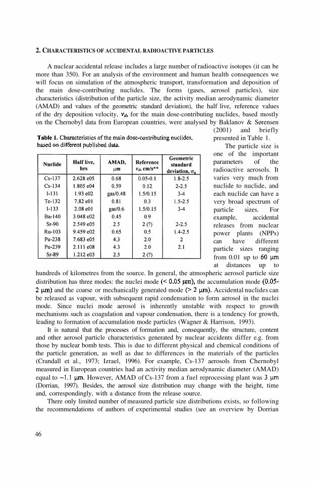
2. CHARACTERISTICS OF ACCIDENTAL RADIOACTIVE PARTICLES
A nuclear accidental release includes a large number of radioactive isotopes (it can bemore than 350). For an analysis of the environment and human health consequences wewill focus on simulation of the atmospheric transport, transformation and deposition ofthe main dose-contributing nuclides. The forms (gases, aerosol particles), sizecharacteristics (distribution of the particle size, the activity median aerodynamic diameter(AMAD) and values of the geometric standard deviation), the half live, reference valuesof the dry deposition velocity, for the main dose-contributing nuclides, based mostlyon the Chernobyl data from European countries, were analysed by Baklanov & Sørensen
(2001) and brieflypresented in Table 1.
The particle size isone of the importantparameters of theradioactive aerosols. Itvaries very much fromnuclide to nuclide, andeach nuclide can have avery broad spectrum ofparticle sizes. Forexample, accidentalreleases from nuclearpower plants (NPPs)can have differentparticle sizes rangingfrom 0.01 up toat distances up to
hundreds of kilometres from the source. In general, the atmospheric aerosol particle sizedistribution has three modes: the nuclei mode the accumulation mode
and the coarse or mechanically generated mode Accidental nuclides canbe released as vapour, with subsequent rapid condensation to form aerosol in the nucleimode. Since nuclei mode aerosol is inherently unstable with respect to growthmechanisms such as coagulation and vapour condensation, there is a tendency for growth,leading to formation of accumulation mode particles (Wagner & Harrison, 1993).
It is natural that the processes of formation and, consequently, the structure, contentand other aerosol particle characteristics generated by nuclear accidents differ e.g. fromthose by nuclear bomb tests. This is due to different physical and chemical conditions ofthe particle generation, as well as due to differences in the materials of the particles(Crandall et al., 1973; Izrael, 1996). For example, Cs-137 aerosols from Chernobylmeasured in European countries had an activity median aerodynamic diameter (AMAD)equal to However, AMAD of Cs-137 from a fuel reprocessing plant was(Dorrian, 1997). Besides, the aerosol size distribution may change with the height, timeand, correspondingly, with a distance from the release source.
There only limited number of measured particle size distributions exists, so followingthe recommendations of authors of experimental studies (see an overview by Dorrian
46

(1997)), we will assume the log-normal distribution of the radionuclide particle size. TheAMAD and the geometric standard deviation can be used for calculation of the log-normal distribution of the nuclide particles. Besides, the particle density, is importantfor the deposition and it can vary for different nuclides, e.g. for Cs-137,but for particles of I-131. Radioactive aerosols differ from other aerosols inthat they are capable of charging themselves directly by the emission of charged particles.
3. AEROSOL TRANSFORMATION PROCESSES
In general, the processes of nucleation, condensation and coagulation can play animportant role in the formation and transformation of atmospheric radioactive aerosols.
3.1 Nucleation and condensation processes
Some nuclides can transform from a gaseous to particulate form. For example, it isvery important for I-131, wich can be released in different forms (molecular, organic andparticles). The gaseous form of I-131 usually dominates in releases (more than 90 %).However, the gaseous iodine has a significant tendency to become attached to otherparticles (usually to particles). This is not a one-way process, there is a strongtendency for the effective deposition velocity to decrease with time.
Iodine nuclei mode particles are the product of vapour condensation and gas-to-particle conversion processes. The last transformations happen due to the nucleationprocesses as well. Nucleation is the formation of a new stable embryonic particle ordroplet which is capable of growth by condensation. The nucleation and condensationprocesses can be simulated by corresponding kinetic equations (e.g. Jacobson, 1999).However, this is very difficult to realise for iodines, because both the homogeneous andheterogeneous (with other existing ambient aerosol particles) nucleations are important,as well as chemical processes. So, as a first approximation, this can be described in themodel by a depletion equation (Maryon et al., 1992):
where c and are concentrations of the particle and gas phases, and are thegaseous and particulate deposition velocities, h is the mixing height and is a timescaleestimated to 47 days from the gaseous/particulate ratio measured after Chernobyl.
However, for main modelling items the prediction time is much shorter (up to 5-7days), therefore it is possible to simulate the deposition of iodines with the time-independent deposition velocities, but separately for the gaseous and particulate forms. Inthis case we have to know the I-131 releases for each form. For the gaseous forms of I-131 the reference values for are 1.5 cm/s for the elemental iodine and 0.015 cm/s forthe organic bound iodine. For the particle form is correspondent to the dry depositionvelocity for and equal to ~ 0.15 cm/s.
47
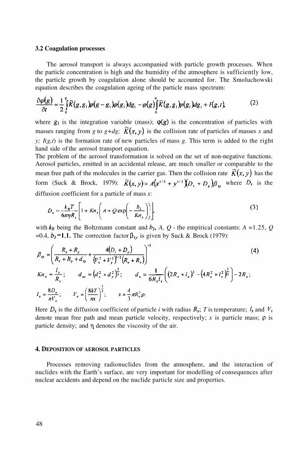
3.2 Coagulation processes
The aerosol transport is always accompanied with particle growth processes. Whenthe particle concentration is high and the humidity of the atmosphere is sufficiently low,the particle growth by coagulation alone should be accounted for. The Smoluchowskiequation describes the coagulation ageing of the particle mass spectrum:
where is the integration variable (mass); is the concentration of particles withmasses ranging from g to g+dg; is the collision rate of particles of masses x and
y; I(g,t) is the formation rate of new particles of mass g. This term is added to the righthand side of the aerosol transport equation.The problem of the aerosol transformation is solved on the set of non-negative functions.Aerosol particles, emitted in an accidental release, are much smaller or comparable to the
mean free path of the molecules in the carrier gas. Then the collision rate has the
form (Suck & Brock, 1979): where is the
diffusion coefficient for a particle of mass x:
with being the Boltzmann constant and A, Q - the empirical constants: A =1.25, Q=0.4, The correction factor is given by Suck & Brock (1979):
Here is the diffusion coefficient of particle i with radius T is temperature; anddenote mean free path and mean particle velocity, respectively; x is particle mass; isparticle density; and denotes the viscosity of the air.
4. DEPOSITION OF AEROSOL PARTICLES
Processes removing radionuclides from the atmosphere, and the interaction ofnuclides with the Earth’s surface, are very important for modelling of consequences afternuclear accidents and depend on the nuclide particle size and properties.
48
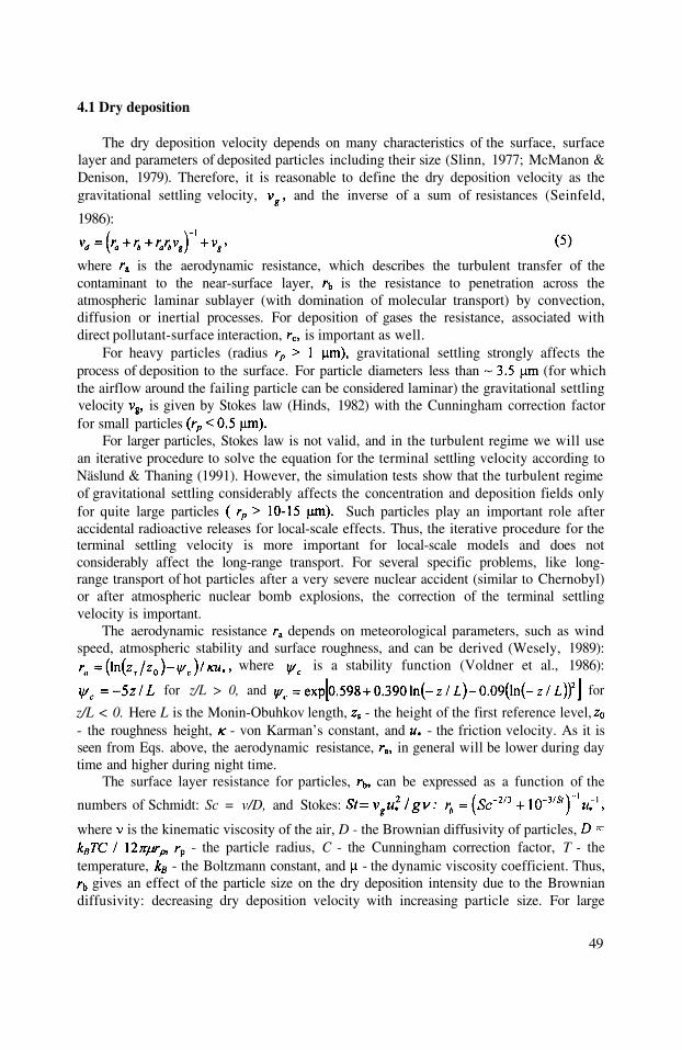
4.1 Dry deposition
The dry deposition velocity depends on many characteristics of the surface, surfacelayer and parameters of deposited particles including their size (Slinn, 1977; McManon &Denison, 1979). Therefore, it is reasonable to define the dry deposition velocity as thegravitational settling velocity, and the inverse of a sum of resistances (Seinfeld,
1986):
where is the aerodynamic resistance, which describes the turbulent transfer of thecontaminant to the near-surface layer, is the resistance to penetration across theatmospheric laminar sublayer (with domination of molecular transport) by convection,diffusion or inertial processes. For deposition of gases the resistance, associated withdirect pollutant-surface interaction, is important as well.
For heavy particles (radius gravitational settling strongly affects theprocess of deposition to the surface. For particle diameters less than (for whichthe airflow around the failing particle can be considered laminar) the gravitational settlingvelocity is given by Stokes law (Hinds, 1982) with the Cunningham correction factorfor small particles
For larger particles, Stokes law is not valid, and in the turbulent regime we will usean iterative procedure to solve the equation for the terminal settling velocity according toNäslund & Thaning (1991). However, the simulation tests show that the turbulent regimeof gravitational settling considerably affects the concentration and deposition fields onlyfor quite large particles Such particles play an important role afteraccidental radioactive releases for local-scale effects. Thus, the iterative procedure for theterminal settling velocity is more important for local-scale models and does notconsiderably affect the long-range transport. For several specific problems, like long-range transport of hot particles after a very severe nuclear accident (similar to Chernobyl)or after atmospheric nuclear bomb explosions, the correction of the terminal settlingvelocity is important.
The aerodynamic resistance depends on meteorological parameters, such as windspeed, atmospheric stability and surface roughness, and can be derived (Wesely, 1989):
where is a stability function (Voldner et al., 1986):
for z/L > 0, and for
z/L < 0. Here L is the Monin-Obuhkov length, - the height of the first reference level,- the roughness height, - von Karman’s constant, and - the friction velocity. As it isseen from Eqs. above, the aerodynamic resistance, in general will be lower during daytime and higher during night time.
The surface layer resistance for particles, can be expressed as a function of the
numbers of Schmidt: Sc = v/D, and Stokes:
where is the kinematic viscosity of the air, D - the Brownian diffusivity of particles,- the particle radius, C - the Cunningham correction factor, T - the
temperature, - the Boltzmann constant, and - the dynamic viscosity coefficient. Thus,gives an effect of the particle size on the dry deposition intensity due to the Brownian
diffusivity: decreasing dry deposition velocity with increasing particle size. For large
49
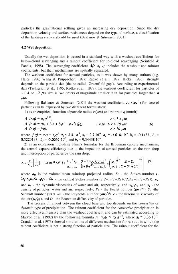
particles the gravitational settling gives an increasing dry deposition. Since the drydeposition velocity and surface resistances depend on the type of surface, a classificationof the land/sea surface should be used (Baklanov & Sørensen, 2001).
4.2 Wet deposition
Usually the wet deposition is treated in a standard way with a washout coefficient forbelow-cloud scavenging and a rainout coefficient for in-cloud scavenging (Seinfeld &Pandis, 1998). The scavenging coefficient includes the washout and rainoutcoefficients, but their mechanisms are spatially separated.
The washout coefficient for aerosol particles, as it was shown by many authors (e.g.Hales 1986; Wang & Pruppacher, 1977; Radke et al., 1977; Hicks, 1976), stronglydepends on the particle size (the so-called ‘Greenfield gap’). According to experimentaldata (Tschiersch et al., 1995; Radke et al., 1977), the washout coefficient for particles of~ 0.4 or size is two orders of magnitude smaller than for particles larger than
Following Baklanov & Sørensen (2001) the washout coefficient, for aerosolparticles can be expressed by two different formulation:
1) as an empirical function of particle radius r and rainrate q (mm/h):
whereand
2) as an expression including Slinn’s formulae for the Brownian capture mechanism,the aerosol capture efficiency due to the impaction of aerosol particles on the rain dropand interception of particles by the rain drop:
where is the volume-mean raindrop projected radius, St - the Stokes number
- the critical Stokes number (1.2+ln(1+Re)/12)/(1+ln(1+Re)),
and - the dynamic viscosities of water and air, respectively, and and - thedensity of particles, water and air, respectively, Pe - the Peclet number Sc -theSchmidt number (v/D), Re - the Reynolds number - the kinematic viscosity ofthe air and D - the Brownian diffusivity of particles.
The process of rainout between the cloud base and top depends on the convective ordynamic type of precipitation. The rainout coefficient for the convective precipitation ismore effective/intensive than the washout coefficient and can be estimated according toMaryon et al. (1992) by the following formula whereCrandall et al. (1973) showed simulations of different mechanism for rainout in which therainout coefficient is not a strong function of particle size. The rainout coefficient for the
50

dynamic precipitation is close to being equal to the washout coefficient, and the rainouteffect in this case can be also estimated by Eq.(6).
The range of values of for snow is 2 - 10 times lower than the washout coefficientfor rain with equivalent precipitation rates. So, we suggest to use the above formulationswith other experimental coefficients (Baklanov & Sørensen, 2001).
5. MODELS FOR AEROSOL DYNAMICS STUDIES
5.1 Eulerian model for local- and meso- scale
For the local- and meso- scale simulation of the radioactive aerosol dynamics the Euleriantype atmospheric aerosol transport model of the Russian Institute of NumericalMathematics was used (Marchuk et al., 1990; Aloyan et al., 1993, 1997). The model ingeneral includes the processes of the nucleation, condensation and coagulation ofaerosols. The aerosol model was off-line coupled with a 3D meso-meteorological modelfor complex terrain (Penenko & Aloyan, 1985; Aloyan & Baklanov, 1985). Thenumerical algorithm is based on the method of splitting of physical processes. On eachsmall time interval the following scheme consisting of these 3 main steps is used: aerosoltransport along trajectories; turbulent diffusion; and coagulation. Full description of thenumerical algorithm and general solution technique can be found in (Marchuk et al.,1990; Aloyan et al., 1997). In given simulations the model did not take into account thenucleation and condensation processes.
5.2 Lagrangian model for long-range transport of aerosols
For the regional scale and long-range transport of radioactive aerosols the DanishEmergency Response Model of the Atmosphere (DERMA) (Sørensen, 1998; Sørensen etal., 1998; Baklanov and Sørensen, 2001) was applied. DERMA, a 3-D Lagrangian long-range dispersion model, using a puff diffusion parameterisation (Sørensen, 1998), isdeveloped at the Danish Meteorological Institute for nuclear emergency preparednesspurposes. Meteorological fields from the operational DMI-HIRLAM model (Saas et al.,1999) were used. Earlier comparisons of simulations by the DERMA model versus theETEX experiment gave very good results. Based on analyses from the first experiment,the among 28 models from most European countries, USA, Canada and Japan, DERMAwas recognised as very successful (Graziani et al., 1998). For the regional scale it will beshown (see discussions below) that the dry and wet deposition processes become moreimportant than the coagulation processes and the effect of the particle size distribution isextremely important. So, the particle size distribution from the local scale modelling isused as an input for the regional scale model.
6. NUMERICAL SIMULATIONS AND DISCUSSION
Let us to discuss some example simulation study for a hypothetical accident releaseof Cs-137 from the Kola NPP with respect to the region of Northern Europe.
51
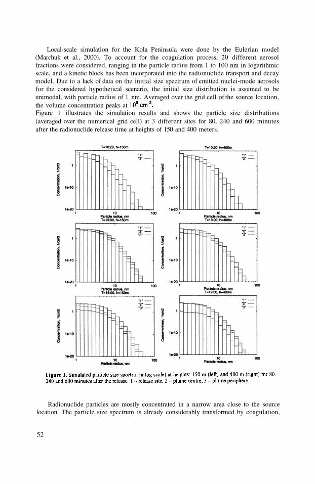
Local-scale simulation for the Kola Peninsula were done by the Eulerian model(Marchuk et al., 2000). To account for the coagulation process, 20 different aerosolfractions were considered, ranging in the particle radius from 1 to 100 nm in logarithmicscale, and a kinetic block has been incorporated into the radionuclide transport and decaymodel. Due to a lack of data on the initial size spectrum of emitted nuclei-mode aerosolsfor the considered hypothetical scenario, the initial size distribution is assumed to beunimodal, with particle radius of 1 nm. Averaged over the grid cell of the source location,the volume concentration peaks atFigure 1 illustrates the simulation results and shows the particle size distributions(averaged over the numerical grid cell) at 3 different sites for 80, 240 and 600 minutesafter the radionuclide release time at heights of 150 and 400 meters.
Radionuclide particles are mostly concentrated in a narrow area close to the sourcelocation. The particle size spectrum is already considerably transformed by coagulation,
52
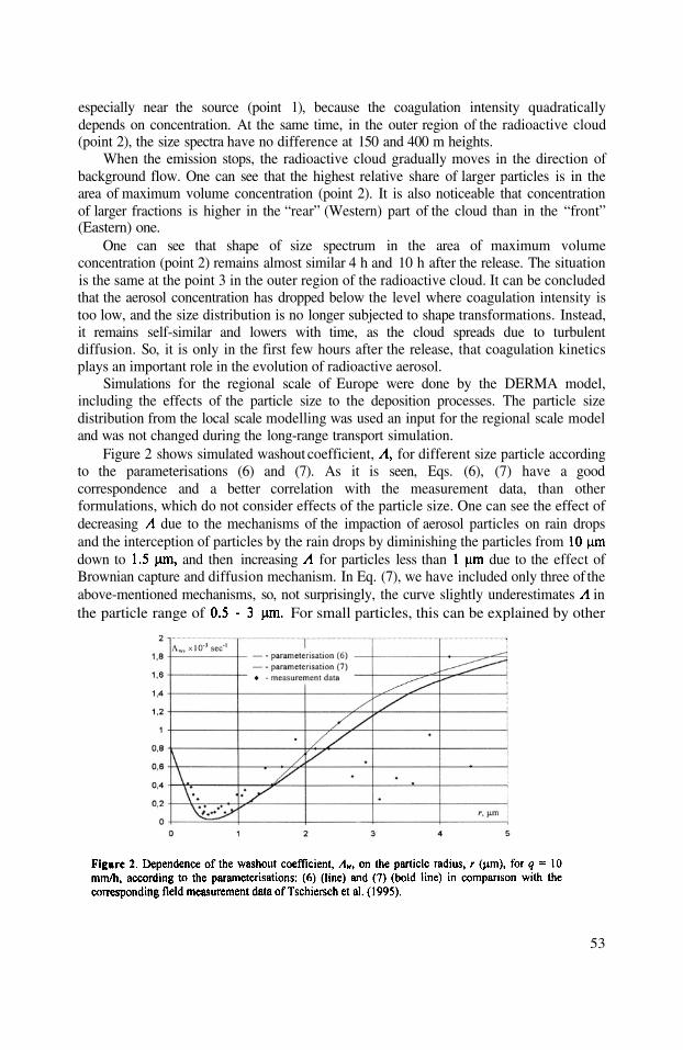
especially near the source (point 1), because the coagulation intensity quadraticallydepends on concentration. At the same time, in the outer region of the radioactive cloud(point 2), the size spectra have no difference at 150 and 400 m heights.
When the emission stops, the radioactive cloud gradually moves in the direction ofbackground flow. One can see that the highest relative share of larger particles is in thearea of maximum volume concentration (point 2). It is also noticeable that concentrationof larger fractions is higher in the “rear” (Western) part of the cloud than in the “front”(Eastern) one.
One can see that shape of size spectrum in the area of maximum volumeconcentration (point 2) remains almost similar 4 h and 10 h after the release. The situationis the same at the point 3 in the outer region of the radioactive cloud. It can be concludedthat the aerosol concentration has dropped below the level where coagulation intensity istoo low, and the size distribution is no longer subjected to shape transformations. Instead,it remains self-similar and lowers with time, as the cloud spreads due to turbulentdiffusion. So, it is only in the first few hours after the release, that coagulation kineticsplays an important role in the evolution of radioactive aerosol.
Simulations for the regional scale of Europe were done by the DERMA model,including the effects of the particle size to the deposition processes. The particle sizedistribution from the local scale modelling was used an input for the regional scale modeland was not changed during the long-range transport simulation.
Figure 2 shows simulated washout coefficient, for different size particle accordingto the parameterisations (6) and (7). As it is seen, Eqs. (6), (7) have a goodcorrespondence and a better correlation with the measurement data, than otherformulations, which do not consider effects of the particle size. One can see the effect ofdecreasing due to the mechanisms of the impaction of aerosol particles on rain dropsand the interception of particles by the rain drops by diminishing the particles fromdown to and then increasing for particles less than due to the effect ofBrownian capture and diffusion mechanism. In Eq. (7), we have included only three of theabove-mentioned mechanisms, so, not surprisingly, the curve slightly underestimates inthe particle range of For small particles, this can be explained by other
53
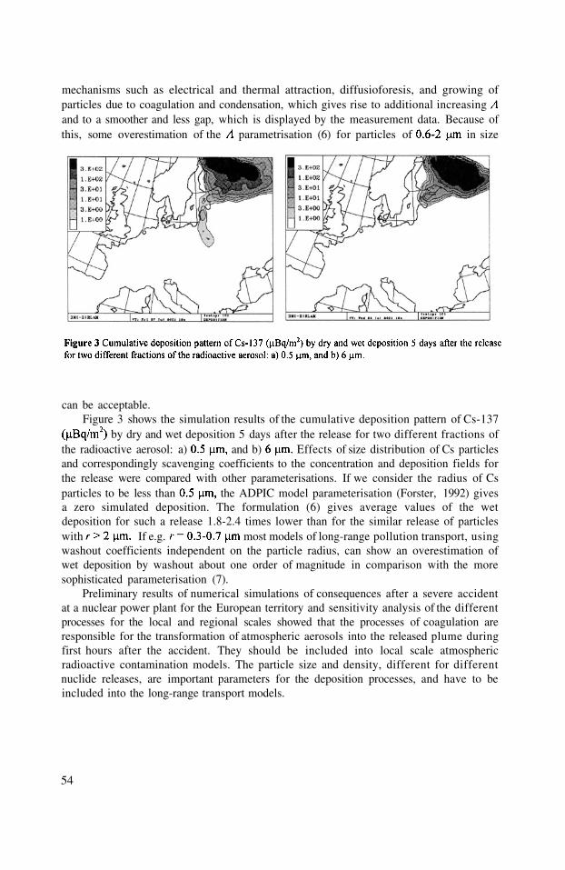
mechanisms such as electrical and thermal attraction, diffusioforesis, and growing ofparticles due to coagulation and condensation, which gives rise to additional increasingand to a smoother and less gap, which is displayed by the measurement data. Because ofthis, some overestimation of the parametrisation (6) for particles of in size
can be acceptable.Figure 3 shows the simulation results of the cumulative deposition pattern of Cs-137
by dry and wet deposition 5 days after the release for two different fractions ofthe radioactive aerosol: a) and b) Effects of size distribution of Cs particlesand correspondingly scavenging coefficients to the concentration and deposition fields forthe release were compared with other parameterisations. If we consider the radius of Csparticles to be less than the ADPIC model parameterisation (Forster, 1992) givesa zero simulated deposition. The formulation (6) gives average values of the wetdeposition for such a release 1.8-2.4 times lower than for the similar release of particleswith If e.g. most models of long-range pollution transport, usingwashout coefficients independent on the particle radius, can show an overestimation ofwet deposition by washout about one order of magnitude in comparison with the moresophisticated parameterisation (7).
Preliminary results of numerical simulations of consequences after a severe accidentat a nuclear power plant for the European territory and sensitivity analysis of the differentprocesses for the local and regional scales showed that the processes of coagulation areresponsible for the transformation of atmospheric aerosols into the released plume duringfirst hours after the accident. They should be included into local scale atmosphericradioactive contamination models. The particle size and density, different for differentnuclide releases, are important parameters for the deposition processes, and have to beincluded into the long-range transport models.
54
ACKNOWLEDGEMENTS
The authors are very grateful to Prof. Marchuk G.I. for very useful advises, to Drs.Arutyunyan V.O., Louzan P.I. (INM) and Sørensen J.H. (DMI) who took part in thesimulations. The study was partly supported by the INTAS-96-1802 project.
REFERENCES
Aloyan, A.E., Arutyunyan, V.O., Lushnikov, A.A., and Zagaynov, V.A., 1997, Transport of coagulating aerosolin the atmosphere. J. Aerosol. Sci., 28: 67-85.
Aloyan, A.E. and Baklanov, A.A., 1985, Modelling of physical processes in atmosphere over complex
topography, In Numerical Methods for Problems in Atmospheric Physics and Environmental Protection
/ed. by Penenko V.V., Novosibirsk, pp 29-44 (in Russian).
Aloyan, A.E., Lushnikov, A.A., Makarenko, S.V., Marchuk, G.I., and Zagainov, V.A., 1993, Mathematical
modelling of the atmospheric aerosol transfer with coagulation taken into account. Russ. J. Num. Anal.
Math. Modelling, 8: 17-30.Baklanov, A. and Sørensen, J.H., 2001, Parameterisation of radionuclide deposition in atmospheric long-range
transport modelling. Physics and Chemistry of the Earth. 13 pp. (in press)
Crandall, W.K., Molenkamp, C.R., Wiliams, A.L., Fulk, M.M. Lange, R. and Knox, J.B., 1973, An
investigation of scavenging of radioactivity from nuclear debris clouds: research in progress. LawrenceLivermore National Laboratory, California, USA, Report UCRL-51328.
Dorrian, M.-D., 1997, Particle size distributions of radioactive aerosols in the environment. Radiation
Protection Dosimetry, 69 (2): 117-132.Forster, C. S., ed., 1992, User’s guide to the MATHEW/ADPIC models. UCRL-MA-103581 Rev 1., US LLNL.
Graziani, G., Klug, W., and Mosca, S., 1998, Real-Time Long-Range Dispersion Model Evaluation of the
ETEX first Release (Office for Official Publications of the European Communities, Luxembourg).Hales, J.M., 1986, The mathematical characterisation of precipitation scavenging. In: The Handbook of
Environmental Chemistry / O. Hutzinger, editor, Vol. 4, Part A, pp. 149- 217.Hicks, B.B., 1976, An evaluation of precipitation scavenging rates of background aerosol. Argonne Nat. Lab.
Radiological and Environmental Res. Division Annual Report.Hinds, W.C., 1982, Aerosol Technology. Wiley, New York. pp. 38-68 & 211-232.Izrael, Yu.A., 1996, Nuclear fall-outs after nuclear accidents. S.-Petersburg, Hydrometeoizdat (in Russian)
Jacobson, M.Z., 1999, Fundamentals of atmospheric modeling. Cambridge Univ. Press, 656 p.Marchuk G.I., Aloyan A.E., Lushnikov A.A., and Zagaynov V.A., 1990, Mathematical modelling of aerosol
transport in the atmosphere with regard for coagulation. Prep. DNM. USSR Acad. Sci., #247 (in Russian).Marchuk, G.I., Aloyan, A.E., Arutyunyan, V.O., Louzan, P.I., 2000, Modelling of the Regional and Global
Transport of Radionuclides from the Kola NPP. (ed. R. Bergman) FOA-R-99-01390-861--SEMaryon, R.H., Smith, F.B., Conwy, B.J. and Goddard, D.M., 1992, The U.K. nuclear accident model. Progress
in nuclear energy. 26 (2): 85-104.McManon, T.A. and Denison, P.J., 1979, Empirical atmospheric deposition parameters - a survey. Atmos.
Environ., 13: 571-585.Näslund, E and Thaning, L., 1991, On the settling velocity in a nonstationary atmosphere. Aerosol Science and
Technology, 14: 247-256.Penenko, V.V. and Aloyan, A.E., 1985, Models and Methods for Environmental Problems. Nauka, Moscow.
Radke, L.F., Hindman, E.E. II, Hobbs, V.P., 1977, A case study of rain scavenging of aerosol particles from anindustrial plume. Proc. Symp. On Precipitation Scavenging, 1974. ERDA Symp. Series. NTIS, pp. 425-
436.
55

Saas, B.H., Nielsen, N.W., Jørgensen, J.U. and Amstrup, B., 1999, The operational DMI-HIRLAM system.
DMI technical report #99-21.Seinfeld, J.H. and Pandis, S.N., 1998, Atmospheric chemistry and physics. A Wiley-Interscience public. 1326p.Slinn, W.G.N., 1977, Approximations for the wet and dry removal of particles and gases from the atmosphere.
Water, Air and Soil Pollution, 7, 513.Suck, S.H. and Brock, J.R., 1979, Evolution of atmospheric aerosol particle size distribution via Brownian
coagulation: numerical simulation. J. Aerosol Sci., 10: 581-590.Sørensen, J.H., 1998, Sensitivity of the DERMA Long-Range Gaussian Dispersion Model to Meteorological
Input and Diffusion Parameters. Atmos. Environ. 32: 4195-4206.Sørensen, J.H., Rasmussen, A., Ellermann, T., and Lyck, E., 1998, Mesoscale influence on long-range transport
- Evidence from ETEX modelling and observations, Atmos. Environ. 32: 4207-4217.Tschiersch, J., Trautner, F. and Frank, G., 1995, Deposition of atmospheric aerosol by rain and fog. In: EC
‘Radiation Protection’ Report # EUR 16604 EN, pp. 3-11.Voldner, E.C., Barrie, L.A. and Sirois, A., 1986, A literature review of dry deposition of oxides of sulfur and
nitrogen with emphasis on long-range transport modeling in North America. Atmos. Environ. 20: 2101-2123.
Wang, P.K. and Pruppacher, H.R., 1977, An experimental determination of efficiency with which aerosolparticles are collected by water drops in subsaturated air. J. Atmos. Sci., 34: 1664-1669.
Warner, S.F. and Harrison, R.M. Editors, 1993, Radioecology after Chernobyl: Biogeochemical Pathways of
Artificial radionuclides. SCOPE 50. John Wiley & Sons.Wesely, M.L., 1989, Parametrisation of surface resistances to gaseous dry deposition in regional scale
numerical models. Atm. Environ. 23 (6): 1293-1304.
56

DISCUSSION
B. FISHER
A. BAKLANOV
The model relies on a description of coagulation. How much isknown the mechanism of coagulation of particles and what werethe reasons leading to the preferred method of parameterisation?There is a problem of numerical diffusion depending on thenumber and size of the particle spectra chosen.
The coagulation mechanism is quite known for aerosol particles,at least due to Brownian and turbulent motions. In this study weused some approximation for a rough assessment of theimportance of the coagulation mechanism in the atmosphericaerosol dynamics. For solution of the Smoluchowski equationkernels of coagulation, close to the reality, were chosen. Theyconsider transitions from one collision regime to other (thecontinuum, free-molecular and transition regimes), depending onthe Knudsen number, Kn. The coagulation model in a finite-different form possesses the mass conservation property and has aminimal numerical diffusion. So, the chosen coagulation model isone of advanced in the present time. The gravitational coagulationwas not considered in the calculations due to small size ofconsidered particles. Of course, we understand that there are manyproblems in careful simulation of the coagulation processes, it is,actually, the first attempt to include the coagulation mechanism inmodelling of atmospheric radioactive aerosol dynamics. As nextstep we start to consider the electrical forces, which can beimportant for the coagulation of radionuclide particles, howeverthis effect is not included in this study.
E. GENIKHOVICH The mixing height, h, is a governing parameter in the Maryonequation for depletion. Don’t you think that this equation shouldbe used to concentrations averaged over the height rather than totheir local values?
A. BAKLANOV This simple equation is used only in the long-ranger transportmodel, which accepts the hypotheses of the complete mixing inthe boundary layer (see the paper text). So, this equation is used ina right way. For the local scale model, more complex equationsfor the binary nucleation and further condensation growing ofparticles are realised, but in the given study they were notconsidered due to too slow process of the nucleation for Iodine (T~ 47 days).
57

This page intentionally left blank
AIR QUALITY STUDY OVER THE ATLANTIC COASTOF IBERIAN PENINSULA
Ana C. Carvalho, Anabela Carvalho, Alexandra Monteiro, CarlosBorrego, Ana I. Miranda, Ivan R. Gelpi, Vicent Pérez-Muñuzuri, Maria R.Méndez, and José A. Souto*
ABSTRACT
The west coast of Iberian Peninsula, surrounded by the Atlantic Ocean, ischaracterized by complex topography and some favourable synoptical situations, whichimply the appearance of mesoscale circulations strongly influencing the transport ofpollutants. On the other hand, the regions of Galicia (NW Spain), and the North ofPortugal, have important air pollutants sources (power plants, chemical industries, trafficand biogenic emissions), all of them contributing to the air quality along the Atlanticcoast and even affecting the centre of the Iberian Peninsula.
In order to achieve the proposed objectives, a hierarchy of models was applied: theresults of a global numerical weather prediction model (GCM), namely the AVN(Aviation model from the National Centres for Environmental Prediction of USA) wereused as initial and boundary conditions into the regional meteorological model of thePennsylvania State University/ National Center for Atmospheric Research MesoscaleMeteorology Model (MM5) over an area that includes a large part of the IberianPeninsula, using its nesting capabilities. To analyse the photochemical production overthe fine grid domains an interface between the MM5 and a photochemical model(MARS) was built up, constituting an innovative approach and a first attempt to integratethese two models.
The achieved results must be considered as preliminary, since the application of thisparticular prognostic numerical system indicates that more refinement on the boundarylayer parameterisations as well on the initial and boundary conditions applied to theMARS model is needed, although the systems represents quite well the ozone measuredconcentrations.
Ana C. Carvalho, Anabela Carvalho, Alexandra Monteiro, Carlos Borrego, Ana I. Miranda, Department ofEnvironment and Planning, University of Aveiro, 3810-193 Aveiro, Portugal. Ivan R. Gelpi, Vicent Pérez-Muñuzuri, Faculty of Physics, University of Santiago de Compostela, 15706 Santiago de Compostela, Spain.Maria R. Méndez, and José A. Souto, Department of Chemical Engineering, University of Santiago deCompostela, 15706 Santiago de Compostela, Spain.
*
Air Pollution Modeling and Its Application XV, Edited byBorrego and Schayes, Kluwer Academic/Plenum Publishers, New York, 2002 59

1. INTRODUCTION
Studies on atmospheric circulations over the Iberian Peninsula have shownparticularities concerning summer dynamics (Millan et al., 1992). Frequently, there is thedevelopment of a low thermal pressure area in the centre of the Peninsula, which allowsmesoscale processes enhancement such as land-sea breezes. This type of circulationsencourages photochemical production of air pollutants leading to smog episodes, whichcan cause health problems to the population and environmental degradation.
Global numerical weather prediction can provide information about the present andtime evolution of the atmospheric situation (wind speed, wind direction, temperature,humidity, etc.). This information is fundamental to estimate the transport, production,dispersion and removal of air pollutants.
Nevertheless, global meteorological models are not suitable for regional studies oftransport of pollutants due to their coarse resolution These models do notsimulate properly mesoscale and regional phenomena, but their results may be refinedwith mesoscale models using dynamical downscaling. In dynamical downscaling, GCMsimulations are used to drive regional climate models (RCMs), which simulate mesoscalecirculation and physical processes in the land-atmosphere system. The knowledge andcharacterisation of mesoscale atmospheric flow patterns, as well as, the description, bymathematical models, of dispersion and transformation mechanisms of photo-oxidantsare fundamental.
The main purpose of this work is to describe the application of two numericalsystems: meteorological model (MM5) (Grell et al., 1995) and the air quality model(MARS) (Moussiopoulos, 1992). These systems simulated the dispersion of pollutants inthe atmosphere, during two summer days, in North part of Portugal. It is important tomention that the achieved results should be considered as pilot, because MARS model isvery sensible to the initial and lateral conditions of chemical species concentrations aswell as to the selected MM5 parameterisations. This represents a considerable field ofresearch in order to better integrate both models.
2. THE APPLIED NUMERICAL SYSTEMS: MM5/MARS
Version 3 of the Pennsylvania State University/ National Center for AtmosphericResearch Mesoscale Meteorology Model (MM5V3.4), is a powerful meteorology modelthat contains comprehensive descriptions of atmospheric motions; pressure, moisture, andtemperature fields; momentum, moisture, and heat fluxes; turbulence, cloud formation,precipitation, and atmospheric radiative characteristics.
MM5 is a non-hydrostatic prognostic model with a multiple nesting capability,applying one way or two-way nesting. The most interesting features of MM5V3.4 arerelated with its different physics parameterisations that can be selected by the user andbeing capable of running in different computational platforms (Dudhia et al., 2001).
MARS model describes the dispersion and chemical transformation of air pollutantsin a three dimensional region (Moussiopoulos, 1992). This model is directed towards thephoto-oxidants simulation, from which ozone is the major component. It is a fullyvectorised model that solves the concentration parabolic equation system for knownmeteorological variables. KOREM and RADM2 can be used on MARS as chemical
60
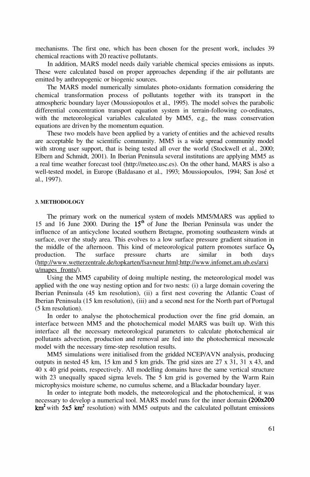
mechanisms. The first one, which has been chosen for the present work, includes 39chemical reactions with 20 reactive pollutants.
In addition, MARS model needs daily variable chemical species emissions as inputs.These were calculated based on proper approaches depending if the air pollutants areemitted by anthropogenic or biogenic sources.
The MARS model numerically simulates photo-oxidants formation considering thechemical transformation process of pollutants together with its transport in theatmospheric boundary layer (Moussiopoulos et al., 1995). The model solves the parabolicdifferential concentration transport equation system in terrain-following co-ordinates,with the meteorological variables calculated by MM5, e.g., the mass conservationequations are driven by the momentum equation.
These two models have been applied by a variety of entities and the achieved resultsare acceptable by the scientific community. MM5 is a wide spread community modelwith strong user support, that is being tested all over the world (Stockwell et al., 2000;Elbern and Schmidt, 2001). In Iberian Peninsula several institutions are applying MM5 asa real time weather forecast tool (http://meteo.usc.es). On the other hand, MARS is also awell-tested model, in Europe (Baldasano et al., 1993; Moussiopoulos, 1994; San José etal., 1997).
3. METHODOLOGY
The primary work on the numerical system of models MM5/MARS was applied to15 and 16 June 2000. During the of June the Iberian Peninsula was under theinfluence of an anticyclone located southern Bretagne, promoting southeastern winds atsurface, over the study area. This evolves to a low surface pressure gradient situation inthe middle of the afternoon. This kind of meteorological pattern promotes surfaceproduction. The surface pressure charts are similar in both days(http://www.wetterzentrale.de/topkarten/fsavneur.html;http://www.infomet.am.ub.es/arxiu/mapes_ fronts/).
Using the MM5 capability of doing multiple nesting, the meteorological model wasapplied with the one way nesting option and for two nests: (i) a large domain covering theIberian Peninsula (45 km resolution), (ii) a first nest covering the Atlantic Coast ofIberian Peninsula (15 km resolution), (iii) and a second nest for the North part of Portugal(5 km resolution).
In order to analyse the photochemical production over the fine grid domain, aninterface between MM5 and the photochemical model MARS was built up. With thisinterface all the necessary meteorological parameters to calculate photochemical airpollutants advection, production and removal are fed into the photochemical mesoscalemodel with the necessary time-step resolution results.
MM5 simulations were initialised from the gridded NCEP/AVN analysis, producingoutputs in nested 45 km, 15 km and 5 km grids. The grid sizes are 27 x 31, 31 x 43, and40 x 40 grid points, respectively. All modelling domains have the same vertical structurewith 23 unequally spaced sigma levels. The 5 km grid is governed by the Warm Rainmicrophysics moisture scheme, no cumulus scheme, and a Blackadar boundary layer.
In order to integrate both models, the meteorological and the photochemical, it wasnecessary to develop a numerical tool. MARS model runs for the inner domain
with resolution) with MM5 outputs and the calculated pollutant emissions
61

grid. Anthropogenic emissions were calculated applying a disaggregation technique fromthe national level to the municipal and them to the sub-municipal level. The CORINAIR95 National Inventory was used to estimate emission data with required spatial andtemporal resolution. For this purpose, disaggregation technique based on statisticalindicators was applied. As a first step, national emission data are disaggregated to themunicipal level using fuel consumption. Then, the data are processed jointly withpopulation statistics in order to obtain sub-municipal resolution. In this work biogenicemissions were not considered.
4. RESULTS AND DISCUSSION
For the present study, ozone measurements were available at three different locationsover the study region (see Figure 1): Coimbra, Avanca and Teixugueira. Coimbra is anurban air quality station and, for this reason, maximum ozone concentrations were
and both occurring at noon of the and of June, 2000. On theother hand, Avanca and Teixugueira air quality stations are located near the industrialcomplex of Estarreja and both present the ozone pick during the afternoon, around 17hand 18h local time, over (see Figure 2). The appearance time of these twopicks, on both days, indicates that the ozone present in these locations may be due toplume production and advection from urban areas, Oporto and/or Coimbra.
62
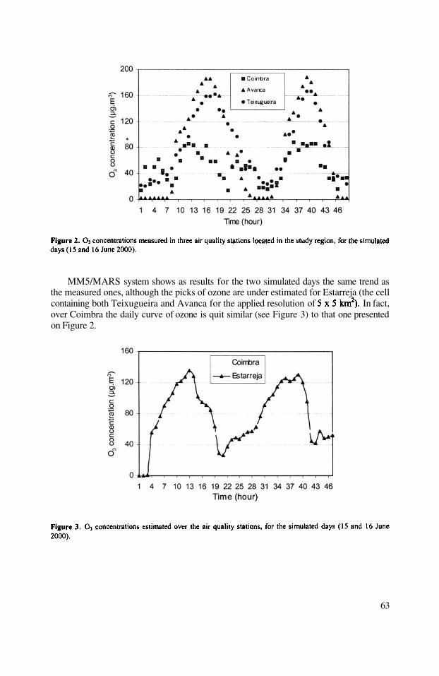
MM5/MARS system shows as results for the two simulated days the same trend asthe measured ones, although the picks of ozone are under estimated for Estarreja (the cellcontaining both Teixugueira and Avanca for the applied resolution of In fact,over Coimbra the daily curve of ozone is quit similar (see Figure 3) to that one presentedon Figure 2.
63
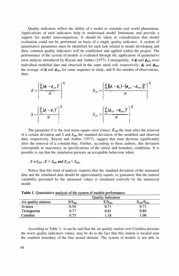
Quality indicators reflect the ability of a model to simulate real world phenomena.Applications of such indicators help to understand model limitations and provide asupport for model intercomparison. It should be taken in consideration that modelevaluation could not be performed on basis of a single quality indicator. A system ofquantitative parameters must be identified for each task related to model developing andthen, common quality indicators will be established and applied within the project. Theperformance of the system of models is evaluated through the application of quantitativeerror analysis introduced by Keyser and Anthes (1977). Consequently, if and wereindividual modelled data and observed in the same mesh cell, respectively; andthe average of and for some sequence in study, and N the number of observations,then:
The parameter E is the root mean square error (rmse), the rmse after the removalof a certain deviation and S and the standard deviation of the modelled and observeddata, respectively. Keyser and Anthes (1977), suggest that rmse decrease significantlyafter the removal of a constant bias. Further, according to these authors, this deviationcorresponds to inaccuracy in specifications of the initial and boundary conditions. It ispossible to say that the simulation presents an acceptable behaviour when:
Notice that this kind of analysis requires that the standard deviation of the measureddata and the simulated data should be approximately equals, to guarantee that the naturalvariability presented by the measured values is simulated correctly by the numericalmodel.
According to Table 1, it can be said that the air quality station over Coimbra presentsthe worst quality indicators values, may be do to the fact that this station is located nearthe southern boundary of the fine nested domain. The system of models is not able to
64
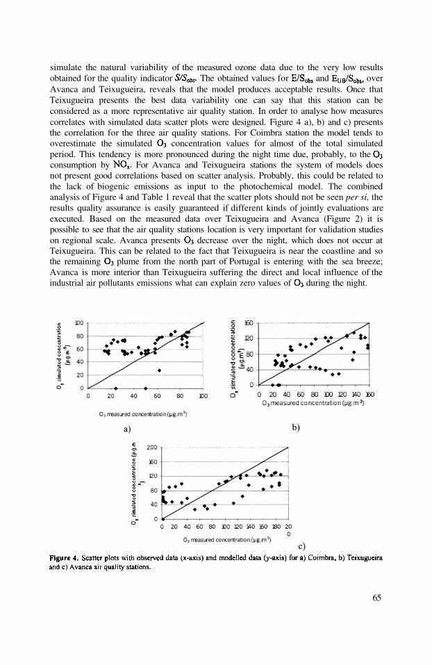
simulate the natural variability of the measured ozone data due to the very low resultsobtained for the quality indicator The obtained values for and overAvanca and Teixugueira, reveals that the model produces acceptable results. Once thatTeixugueira presents the best data variability one can say that this station can beconsidered as a more representative air quality station. In order to analyse how measurescorrelates with simulated data scatter plots were designed. Figure 4 a), b) and c) presentsthe correlation for the three air quality stations. For Coimbra station the model tends tooverestimate the simulated concentration values for almost of the total simulatedperiod. This tendency is more pronounced during the night time due, probably, to theconsumption by For Avanca and Teixugueira stations the system of models doesnot present good correlations based on scatter analysis. Probably, this could be related tothe lack of biogenic emissions as input to the photochemical model. The combinedanalysis of Figure 4 and Table 1 reveal that the scatter plots should not be seen per si, theresults quality assurance is easily guaranteed if different kinds of jointly evaluations areexecuted. Based on the measured data over Teixugueira and Avanca (Figure 2) it ispossible to see that the air quality stations location is very important for validation studieson regional scale. Avanca presents decrease over the night, which does not occur atTeixugueira. This can be related to the fact that Teixugueira is near the coastline and sothe remaining plume from the north part of Portugal is entering with the sea breeze;Avanca is more interior than Teixugueira suffering the direct and local influence of theindustrial air pollutants emissions what can explain zero values of during the night.
65

5. CONCLUSIONS
Although major problems on the integration of these two models did not appeared inthis first approach of integration, from this work it can be said that it will be fundamentalto validate the meteorological part of the system with the necessary quality indicators. Onthe other hand, biogenic emissions should be considered and chemical species values onboundary conditions are now under evaluation.
6. ACKNOWLEDGEMENTS
The authors wish to thank the PRAXIS XXI (Foundation for Science andTechnology) for the PhD grant of A. C. Carvalho and the European Commission, in thescope of CLIMED project, for the MSc grant of Anabela Carvalho. The authors are alsogratefully acknowledged to the Portuguese Environmental Regional Directorate of theCentre for the accessibility to the measured air quality data. Financial support by theAcción Integrada España-Portugal HP1999-0057 is as well grateful acknowledged.
7. REFERENCES
Baldasano, J. M., Costa, M., Cremades, L., Flassak, T., and Wortmann-Vierthaler, M., 1993, Influence of trafficconditions on the air quality of Barcelona during the Olympic Games’92, in: Air pollution Modelling andIts Application X, S. Gryning & M.M. Millán, eds., Plenum Press, New York, pp. 643-644.
Dudhia, J., Gill, D., Guo, Y., Manning, K., and Wang, W., 2001, PSU/NCAR Mesoscale Modeling SystemTutorial Class Notes and User’s Guide: MM5 Modeling System Version 3, Boulder (June 18, 2001);http://www.mmm.ucar.edu/mm5/.
Elbern, H., and Schmidt, H., 2001, Ozone episode analysis by four-dimensional variational chemistry dataassimilation. Journal of Geophysical Research. 106.
Grell, G., Dudhia, J., and Stauffer, D., 1995, A Description of Fifth-Generation Penn State/NCAR MesoscaleModel (MM5), NCAR Tech. Note NCAR/TN-398+STR, Boulder, pp. 122.
Keyser, D. and Anthes, R.A., 1977, The applicability of a mixed-layer model of the planetary boundary layer toreal-data forecasting. Mon. Weather Rev., Vol. 105, pp. 1351 -1371.
Millan, M., Artinano, B., Alonso, L., Castro, M., Fernandez-Patier, R., and Goberna, J., 1992,Mesometeorological Cycles of Air Pollution in the Iberian Peninsula. Air Pollution Research Report 44,European Community Commission, Brussels.
Moussiopoulos, N., 1992, MARS (model for the Atmospheric Dispersion of Reactive Species): TechnicalReference, Aristotle University, Thessaloniki.
Moussiopoulos, N., 1994, Air pollution modelling in southern Europe, in: Proceedings of EUROTRACSymposium 94, Borrell et al., ed., Academic Publishing, The Hague, pp. 48-55.
Moussiopoulos, N., Sahm, P., and Kessler, C., 1995, Numerical simulation of photochemical smog formation inAthens, Greece: a case study. Atmospheric Environment, 29.
San José, R., Pietro, J.F., Martín, J., Delgado, L., Jimenez, E., and González, R.M., 1997, Integratedenvironmental monitoring, forecast and warning systems in metropolitan areas (EMMA): Madridapplication, in: International Conference on Measurements and Modelling in Environmental Pollution,R. San José & C.A. Brebbia, Computational Mechanics Publications, Southampton, pp. 313-323.
Stockwell, W., Koracion, D., Klaic, Z. B., and McCord, T. E., 2000, Modeling of ozone, nitrogen oxides andparticles in the American northwest, in: Seventh International Conference on Atmospheric Sciences andApplications to Air Quality and Exhibition, Taipei, pp. 190.
66
DISCUSSION
Z. WANG
A.I. MIRANDA
1) What is the vertical co-ordinate of MARS ? Is it the same as inMM5 or RAMS ? And how much errors do you expect in thetransformation between MM5 meteorological output to MARS ?How do you deal with the vertical diffusions coefficients inMARS ? Is it directly from MM5 or calculated by MARS ?
1)
2)
MARS has terrain following coordinates based on Cartesiancoordinate system and vertical resolution with non-equidistantlayers. Errors will appear due to the transformation between theArakawa B grid of MM5 and C grid of MARS.Main feature of MARS is the coupled implicit treatment ofvertical diffusion and chemical kinetics.
P. SUPAN Have you also thought to use another photochemical model thanMARS (to improve the results) ?
A.I. MIRANDA For the study region MARS presents suitable performance using themesometeorological MEMO model (with 3D results) so, the mainproblem is related to MM5 model outputs. Outputs improvementshould be done firstly on MM5 runs, and this can be achievedthrough objective analysis.
D.A. STEYN Your modelling system overestimates ozone concentrations at night.This is probably because it underestimates scavenging becausethe meteorological model does not capture surface based radiativetemperature inversions due to insufficient vertical grid resolution.Could this be the case ?
A.I. MIRANDA Although, your guideline is true, in this particular study this is not ajustification because scavenging is not underestimated. Themain problem could be related to fixed air quality boundaryconditions, namely for concentration (30 ppb).
67
2)

F. LEFEBRE
A.I. MIRANDA
Did you perform any sensitivity experiments to the value of theinitial concentration ?
No, we did not.
68
A 3-D atmospheric transport model in a regional scale was used to simulate the leadconcentrations and depositions over North America following a discrete ordinate (DO)method (Daggupaty and Ma, 1998). The lead emission inventories to the atmospherewere developed for Canadian sources from NPRI (National Pollutant Release Inventory,Environment Canada) data set and for U.S. sources from TRI (Toxic Release InventoryUSEPA) data set. These data sets were implemented in the model runs.
Objectively analyzed and predicted meteorological data at 6 hourly data sets fromGlobal Environmental Multi-scale model (GEM) of CMC (Canadian MeteorologicalCenter) and a fine scale boundary layer physics module were utilized to drive theatmospheric transport and deposition model. The model domain covers central andeastern parts of Canada and United States. The model has 10 non-uniformly spaced levelsin the vertical, extended from the surface to the height at 3 km. The horizontal grid scaleof the model is 35 km with total of 90×90-grid points.
*ARQI, Meteorological service of Canada, 4905 Dufferin Street, Downsview, Ontario, Canada. M3H 5T4Tel: 416-739-4451, Fax: 416-739-4288; e-mail: [email protected]
NUMERICALLY SIMULATED ATMOSPHERICTRANSBOUNDARY CONTRIBUTION OF LEAD
LOADING TO THE GREAT LAKES.
Sreerama M. Daggupaty and Jianmin Ma *
1. INTRODUCTION
Atmospheric deposition of lead is one of the significant sources of toxicpollutants entering the Great Lakes. In fact, as much as 90 percent of some toxic loadingsto the Great Lakes are believed to be the result of airborne deposition. Because thephenomenon of transport and deposition of airborne toxics is not localized, the problemneeds to be evaluated and regulated at least on a regional scale. The purpose of this studyis to investigate the contributions of industrial emission sources of lead from parts ofCanada and United States to the Great Lakes.
2. NUMERICAL MODEL
Air Pollution Modeling and Its Application XV, Edited byBorrego and Schayes, Kluwer Academic/Plenum Publishers, New York, 2002 69

An “effective” dry deposition velocity (Ma and Daggupaty, 2000), which considersthe effects of the sub-grid scale surface categories on the heavy metal deposition, wasdeveloped and implemented in the model. The wet deposition was computed using thescheme according to Bartnicki et al (1993). The precipitation data used in thecomputation of wet deposition was from the predicted hourly precipitation rate of CMC’sGEM model.
Figures 1 and 2 display modeled yearly total deposition (dry deposition + wetdeposition) in 1995 due to Canadian (NPRI) and US (TRI) emissions respectively. Aninteresting feature is that there exists a gradient in deposition over the lakes, reflecting theproximity of sources and atmospheric transport. Such sub-lake features are also evidentfor the modeled air concentration through numerical simulation. This underscores theinadequacy of estimating deposition by assuming a single monitored concentration from
70
3. RESULTS AND DISCUSSIONS
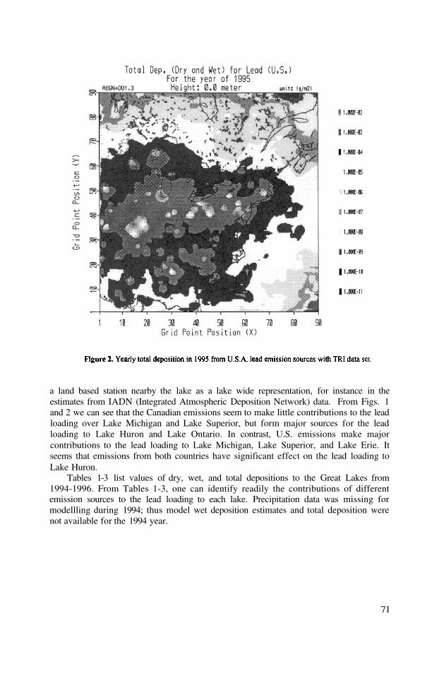
a land based station nearby the lake as a lake wide representation, for instance in theestimates from IADN (Integrated Atmospheric Deposition Network) data. From Figs. 1and 2 we can see that the Canadian emissions seem to make little contributions to the leadloading over Lake Michigan and Lake Superior, but form major sources for the leadloading to Lake Huron and Lake Ontario. In contrast, U.S. emissions make majorcontributions to the lead loading to Lake Michigan, Lake Superior, and Lake Erie. Itseems that emissions from both countries have significant effect on the lead loading toLake Huron.
Tables 1-3 list values of dry, wet, and total depositions to the Great Lakes from1994-1996. From Tables 1-3, one can identify readily the contributions of differentemission sources to the lead loading to each lake. Precipitation data was missing formodellling during 1994; thus model wet deposition estimates and total deposition werenot available for the 1994 year.
71

A comparison of Tables 1, 2, and 3 indicates that the U.S sources contribute about85% of the dry deposition over Lake Erie in 1994, about 87% and 95% in 1995 and 1996respectively. For the wet deposition, the lead emissions from United States account toabout 88% in 1995 and 94% in 1996. This implies that about 87% in 1995 and 95% in1996 of the total lead loading to Lake Erie are due to the emissions from United States.Similarly, U. S. sources also make the most contributions to lead loading to LakeMichigan, whilst the deposition over Lake Michigan due to the emissions from Canadacan be ignored. It is interesting to see that the U.S. sources account to quite large amountof deposition in Lake Superior in 1994 and 1995 compared with Canadian sources. In1996, however, the depositions over Lake Superior due to the emissions from UnitedStates are reduced considerably. However still 50% of the total deposition is due to USsources. Although both United States and Canada have emission sources near the LakeOntario, it is clear from Tables 2 and 3 that Canadian sources lead to larger amount ofdepositions over Lake Ontario. In 1995 and 1996, the total depositions are 86% and 84%respectively due to Canadian sources.
72
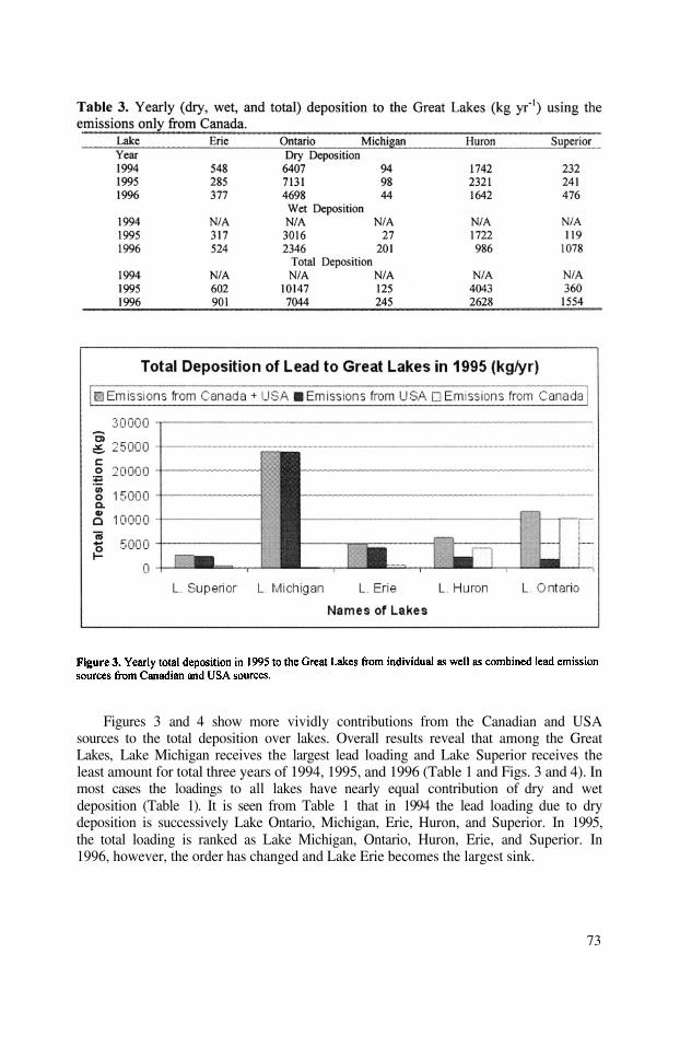
Figures 3 and 4 show more vividly contributions from the Canadian and USAsources to the total deposition over lakes. Overall results reveal that among the GreatLakes, Lake Michigan receives the largest lead loading and Lake Superior receives theleast amount for total three years of 1994, 1995, and 1996 (Table 1 and Figs. 3 and 4). Inmost cases the loadings to all lakes have nearly equal contribution of dry and wetdeposition (Table 1). It is seen from Table 1 that in 1994 the lead loading due to drydeposition is successively Lake Ontario, Michigan, Erie, Huron, and Superior. In 1995,the total loading is ranked as Lake Michigan, Ontario, Huron, Erie, and Superior. In1996, however, the order has changed and Lake Erie becomes the largest sink.
73

Changes of lead loading to the Great Lakes are due, except for the meteorologicalconditions, to the reductions of emissions from United States in the vicinity of the GreatLakes in 1996. However in this year the U.S. sources still made major contributions ofthe lead deposition to the Lake Erie, Michigan, and Superior in comparison with theCanadian sources (Fig.4). It is seen (Fig. 4 and Tables 1-3) that the contribution of leadloading to the Lake Erie from U.S sources (TRI) increases drastically in 1996 comparedto 1994 and 1995. In general, the modeled total lead loading to Great Lakes is lower thanthe IADN (Integrated Atmospheric Deposition Network) monitored and estimated data(Hoff et al. 1996). This is mainly due to the model estimated wet depositions areconsiderably lower than the IADN data. Detailed comparison of depositions to the GreatLakes with IADN data will be reported in a future paper.
In order to demonstrate the model performance, we illustrate in Fig. 5, thecomparison of modeled and measured air concentration from IDAN stations at BurntIsland, Egbert, and Pt. Petre in 1995. The comparison was made for sampling days at themonitoring stations with the nearest grid point simulations from the model. Generally atIADN stations once every 12 days the air concentration is monitored for about 24 hours.As shown, the daily averaged predicted surface air concentration is agreeing very wellwith the measured concentration. Preliminary examination of model predicted drydeposition is lower than that estimated by IADN data. IADN’s algorithm of drydeposition uses a constant deposition velocity irrespective of time and surface type. In thecase of the model it is a variable function dependent upon the surface characteristics andtransient boundary layer dynamic parameters. It is possible that IADN estimateddepositions whether dry or wet are not truly representing lake wide loadings. The reasonis that IADN estimates are constrained by a single land based monitoring station andhence biased by the conditions at the site.
74

75
Using a 3-D Eulerian atmospheric transport model, the lead loading to the GreatLakes subject to different emission sources were simulated for 1994, 1995, and 1996. Itwas found that the lead emissions from sources in the United States made majorcontributions to the lead loading to the Lakes Erie, Michigan, and Superior, whilst thelead loading to the Lakes Ontario and Huron were determined largely by the emissionsfrom Canada. Overall results reveal that among the Great Lakes, Lake Michigan receivesthe largest lead loading and Lake Superior receives the least amount for total three yearsof 1994, 1995, and 1996. In 1994 and 1995, the lead loadings to the Great Lakes did notchange dramatically. In 1996, however, we noticed significant changes of the leadloadings in several lakes. Among them the Lake Michigan showed significant reductionand the Lake Erie showed apparent increase. These variations are attributed largely to thechanges of the lead emission sources in the United States. Model predicted sub-lakefeatures such as non-uniform air concentration and deposition are noteworthy and suchfeatures have strong repercussions in comparison with the estimates of dry and wetdeposition from land-based monitored data.
Mr. Philip Cheung’s contribution with computer programming and emission datasets is appreciated. Ms. Anita Wong and Mr. Terry Mah are acknowledged for their helpwith NPRI and TRI data sets. We express our sincere thanks to Ms. Celine Audette,IADN officer of MSC for supplying IADN data. We acknowledge the help of Mr. VasuDaggupaty with the figures. We appreciate the encouragement and interest of Dr. KeithPuckett.
Bartnicki J, et al, 1993: An Eulerian model for atmospheric transport of heavy metals over Europe. Techniquereport No. 117, Det Norske Meteorlogiske Institutt.
Hoff R. M., et al., 1996: Atmospheric deposition of toxic chemicals to the Great Lakes: a review of data through1994. Atmospheric Environment, 30, 3505-3527
Ma J. and S. M. Daggupaty, 2000: Effective dry deposition velocities for gases and particles over heterogeneousterrain. J. Appl. Meteorol., 39, 1379-1390.
Daggupaty S. M. and J. Ma, 1998: Discrete ordinate/ Pseudospectral simulations of transport of heavy metalsover regions of North America. joint conference on the application of air pollution meteorology withthe A&WMA. Phoenix, Pre-print volume Amer. Meteor. Soc., January 1998, 410-413.
76
4. CONCLUSIONS
5. ACKNOWLEDGMENTS:
6. REFERENCES

Are the Pb sources primarily Pb smelters ? How is the Pbtransported ? Primarily as aerosol particles, and, if so, in what sizerange ?
These questions need to be answered by the authors, i.e. S.Dagguparty and J. Ma.
77
Yes, the major Pb sources are metal smelting industries, however ourdata base has some other industrial activities that deal with Pb, butthey are minor. It is assumed to be transported as a passive particle.The mean particle size is considered for this study as 0.55um.
DISCUSSION
A. HANSEN
W. GONG
S. DAGGUPARTY

This page intentionally left blank

Increasing traffic density gives rise to problems with air pollution that is met mainlyin summer months – so called summer photochemical smog. Prague can serve as atypical example of a city where traffic density increased several times that situation adecade ago and as the infrastructure is not prepared for such a rapid changes the problemsare quite large. Moreover, as there is no outer ring and also almost all cars passing Praguegoes through its center. This situation is improving now, when parts of the city ring isunder construction or partly finished but still there are missing very important parts ofthis important traffic city system. Prague is not only a historical city and capitol of theCzech Republic, it is also a place with a great concentration of industry and other humanactivity, which leads to problems with air pollution of the above mentioned kind insummer and with nitrogen type of pollution in winter months especially when stagnantcondition occurs.
In this contribution we deal with the problem of summer photochemical smog andthe episodes of high concentration of it. We are mainly interested in its most importantpart – tropospheric ozone. Ground ozone concentration is measured in several monitorsin Prague, but thanks to the complicated orography of Prague and limited number ofmonitors it very problematic to obtain information about spatial distribution of this partof summer photochemical smog based on measured data. Another way how to estimatethis distribution consists in using appropriate model. This approach supposes to use somemeteorological diagnostic or prognostic model (depending on the fact, whether the aim ofthe activity is a diagnostic field of spatial ozone distribution or its forecast) together withchemical submodel involving the whole cycle of chemical reactions. In the subsequentparagraphs the chemical submodel called SMOG is briefly described together with isprepared link to the meteorological model. A future plans dealing with utilization of moredetailed model of higher resolution are also mentioned.
* Tomas Halenka, Josef Brechler, Jan Bednar, Charles University in Prague, Faculty ofMath. and Physics, Prague, Czech Republic
ON THE COUPLING OF AIR-POLLUTION MODEL TONUMERICAL WEATHER PREDICTION MODEL
Tomas Halenka, Josef Brechler, Jan Bednar*
1. INTRODUCTION
Air Pollution Modeling and Its Application XV, Edited byBorrego and Schayes, Kluwer Academic/Plenum Publishers, New York, 2002 79

The presented chemical submodel SMOG (Bednar et al., 2001) has been developedin the framework of the project “Air Pollution in Prague” at the Department ofMeteorology and Environmental Protection, Faculty of Mathematics and Physics, CharlesUniversity in Prague in the period 1995-8. It serves as a tool for studying summerphotochemical smog episodes. Such episodes can be described as a presence of highozone concentration produced by photochemical reactions of its precursors, as nitrogenoxides – and volatile organic compounds – VOC. This high ozone concentration isnot caused only with local conditions (local emission) but it is also a consequence oflong-range transport. In the model SMOG the attempt was based on the methods thattried to estimate the impact of the local city emission on the level of ozone and itprecursors concentrations.
The model has conceptual base in the category of so-called “puff” models. Theprinciple of this type of models consists in hacking of air-pollution plumes into series ofpuffs. Plume is then supplied by sequence of partly overlapped elements drifted by awind flow from a source location down the trajectory. That approach allows to reply torapid changes of meteorological conditions and emissions, however the main advantageof this approach is an ability to involve mixing and mutual chemical reacting parts ofplumes proceeded from different sources.
80
2. CHEMICAL SUBMODEL SMOG

The model chemical reactions can be characterized with the scheme presented inFig. 1. Reactions involved can be written in the form of equations described in detailes inBednar et al. (2001). Usual output of the model involves fields of ground concentrationdistribution of NO, and in Input data that are necessary for running thesubmodel SMOG can be divided into three categories. First category can be called aspermanent or constant information – this category involves data about orography of theinvestigated area (model domain). At this moment so called “US NAVY” orography withresolution 10 × 10 geographic minutes has been used. The second and the third categoryof the data sets consist of emission data and input of meteorological data. Firstly, we willmention emission data in more details as the meteorological data will be discussed in thesection where meteorological prognostic model will be mentioned together withperformed tests of the link between the meteorological model and chemical submodel.
Chemical submodel SMOG has been used for several studies when the grounddistribution of NO, and was computed. Data information on emissions ofand VOC from Prague emission sources and sources from its closest neighbourhood wereinvolved, but there was also information about emission individual (point) sources fromthe whole area of central Bohemia (approximately to the distances of 70 km from thecentre of Prague). The number of involved individual point sources was equal to 177, butthe contribution of sources outside of Prague was relatively negligible. Individual pointsources creates one group of emission sources and these sources are treated in their realpositions with corresponding parameters (building height, emission rate etc.). Model usesalso emission data in gridded form. The whole model domain is divided into regular gridmesh of emission squares (in the above mentioned study the squares 5 × 5 km were used)and all the emissions of and VOC from traffic, area emission sources or small pointemission sources located in a given emission square are attributed to the centre of thissquare. The size of these emission squares is a consequence of a compromise between anattempt to have the most correct emission input and number of puffs that can be treatedwithin one model run as a new puffs is launched from each source each time interval.
Meteorological information consists of data, which are in the first step considered tobe homogeneous in model domain, e.g. surface air temperature, cloud cover, solar zenithangle, total amount of in Dobson units. For wind field vertical changes are taken intoaccount. An example of the results based on homogeneous data in the model domain ispresented in Fig. 2.
If the relatively complicated shape of orography in the Central Bohemia is compared withthe used meteorological data (mainly data about wind field – both speed and direction)then it is evident, that a link to some meteorological “pre-processor” that would createmore realistic flow field is necessary. At least the flow field could display deformationdue to the shape of orography parametrized or modelled in a desired resolution (it meansif the model SMOG is used for simulating the impact of the city plume on thesurrounding areas, then resolution given with up to now used “US NAVY” orography issufficient and flow field could be given in the same resolution). But when the submodel
81
3. LINK TO METEOROLOGICAL CONDITIONS

82
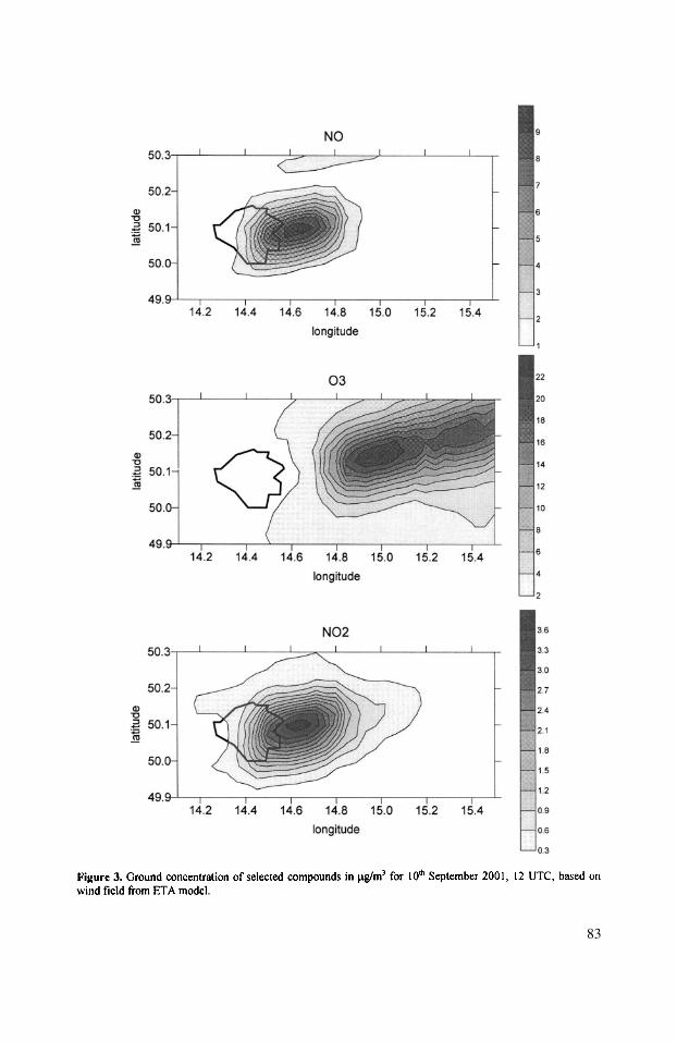
83
SMOG should be used simulating the distribution of ozone concentration in Prague andits closest neighbourhood, then some more detailed information about local terraincondition would be necessary together with some more information, e.g. about thestructure of build-up area, and some high-resolution model should be used as in this casethe local structure of the wind field is consequence of the sum of local conditions actingsimultaneously with large scale meteorological situation.
In the first attempt we used the homogeneous fields as we intended to test ourcoupling routines with meteorological prediction model and the resolution of the modelused was comparable with the scale of the area we were interested in concerning the airpollution transport. Further on, the model we are using for our first experiments with realdriving of our SMOG model is so-called model ETA (Black, 1988) with resolution of0.25 degree. The example of the results is presented in Fig. 3, however, this is not typicalcase of photochemical smog production. Unfortunately mainly the effect of high velocityof wind can be seen there, it should be mentioned that only concentration of producedozone is displayed although the effect of background concentration is parameterised aswell. Moreover, as it is a preliminary study, in this case only trajectories of puffs aredriven by wind field from ETA model taking other parameters to be constant andhomogeneous in the domain. As the second step we are going to fully couple fields ofother parameters like temperature, height of mixing layer, cloudness etc. as well forpurposes of regional air pollution transport modelling. Finally, we are taking into accountthe possibility of experiments with coupling of our chemical submodel to high resolutionmodels MM5 and spectral LAM Aladine.
This study was supported in framework of project GACR 205/01/1120 of the GrantAgency of the Czech Republic. The authors wish to express their thanks for the ETAmodel kindly provided by NCEP.
Bednar, J., Brechler, J., Halenka, T., and Kopacek, J., 2001, Modelling of summer photochemical smog in thePrague region, Phys. Chem. Earth (B), 26, 129-136.
Black, T. L., 1988, The step-mountain eta coordinate regional model: A documentation. National Oceanic andAtmospheric Administration/National Weather Service, p. 47
84
ACKNOWLEDGMENT
REFERENCES

DISCUSSION
Do you take into account the feedback relations between the modelsyou use ?
No, it is one way nesting, i.e. ETA is used just as a meteorologicaldriver or preprocessor and SMOG as a CTM without any feedbackto ETA.
Because of the large differences in chemistry between pointsource plumes and dispersed sources, do you think use of apufmodel may be inappropriate for area sources ?Do puffs originate at regularly gridded points or at pointsources, when they exist ?
Actually, it might be true. However, for more realisticsimulation of city plume we have to include area sources as weare not able to simulate each individual stock or chimney. Thesearea sources are taken into account by means of initial spreadedpuffs with appropriate values of parameter Comparison of themodel simulations with some surface measurements and air-bornplume profiling as well has not given us any strong warmingconcerning this issue till now.Puffs originate at the exact positions of point sources.
85
Vl. PENENKO
T. HALENKA
A. HANSEN 1)
2)
T. HALENKA 1)
2)

This page intentionally left blank

MODELING THE MERCURY CYCLE IN THEMEDITERRANEAN: SIMILARITIES AND
DIFFERENCES WITH CONVENTIONAL AIRPOLLUTION MODELING
G. Kallos, A. Voudouri, I. Pytharoulis and O. Kakaliagou*
Mercury is a toxic metal that is being increasingly recognized as a threat to the healthof numerous wildlife species and tens of thousands of people around the world. Theanthropogenic sources of mercury in the vicinity of the Mediterranean Sea region includepower plants (burning coal and oil), chemical plants (e.g. alkal-cloral plants), wasteincinerators, ferrous foundries, non-ferrous metal smelters, refineries, and cement kilns.Additional contributions of mercury come from two mercury-mining sites in Spain andSlovenia, and 3 volcanoes in Italy. The vast majority of the mercury sources in theMediterranean region are located north of the basin. Hence, they are expected to exert astrong influence on the mercury concentration over the Mediterranean region since theprevailing meteorological conditions favour the transport from north to south. Two mainpaths of transport have been identified in this region (Kallos et al. 1997a). The one path isfrom Eastern Europe toward the Middle East and North Africa while the other one is fromcentral and western Mediterranean toward the east. The first path has been found to be thedominant one.
During the MAMCS project two major model developments were performed. Thesetwo developments were constructed within two well-known atmospheric models: theRegional Atmospheric Modelling System (RAMS; Pielke et al. 1992) and theSKIRON/Eta (Kallos et al. 1997b and references therein). The use of two atmosphericmodels allowed the intercomparison of the results and therefore the better development ofthe mercury modelling system (Kallos et al. 2000). In this development an effort wasmade to transfer and utilize the modeling techniques applied in conventional air pollutionmodelling studies. In addition, we developed new methodologies for processes like re-emissions from soil and water bodies and gas to particle conversion (Pirrone and Keeler,1995). The developed modeling systems have been applied in the Mediterranean Regionwhere the multi-scale atmospheric processes (thermal and mechanical circulations atregional and mesoscale) are considered as important, according to a number of past airpollution studies. Seasonal-type of simulation has been performed for
1. INTRODUCTION
* G. Kallos, A. Voudouri, I. Pytharoulis and O. Kakaliagou, University of Athens, Department of Applied Physics1Panepistimioupolis Bldg Phys V, Athens 15784, GreeceAir Pollution Modeling and Its Application XV, Edited byBorrego and Schayes, Kluwer Academic/Plenum Publishers, New York, 2002 87
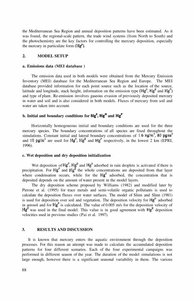
The emission data used in both models were obtained from the Mercury EmissionInventory (MEI) database for the Mediterranean Sea Region and Europe. The MEIdatabase provided information for each point source such as the location of the source,latitude and longitude, stack height, information on the emission type andand type of plant. Re-emission involves gaseous evasion of previously deposited mercuryin water and soil and is also considered in both models. Fluxes of mercury from soil andwater are taken into account.
It is known that mercury enters the aquatic environment through the depositionprocesses. For this reason an attempt was made to calculate the accumulated depositionpatterns for four different scenarios. Each of the four experimental campaigns wasperformed in different season of the year. The duration of the model simulations is notlarge enough, however there is a significant seasonal variability in them. The various
the Mediterranean Sea Region and annual deposition patterns have been estimated. As itwas found, the regional-scale pattern, the trade wind systems (from North to South) andthe photochemistry are the key factors for controlling the mercury deposition, especiallythe mercury in particulate form
2. MODEL SETUP
a. Emissions data (MEI database )
b. Initial and boundary conditions for and
Horizontally homogeneous initial and boundary conditions are used for the threemercury species. The boundary concentrations of all species are fixed throughout thesimulations. Constant initial and lateral boundary concentrations ofand are used for and respectively, in the lowest 2 km (EPRI,1996).
c. Wet deposition and dry deposition initialization
Wet deposition of and adsorbed in rain droplets is activated if there isprecipitation. For and the whole concentrations are deposited from that layerwhere condensation occurs, while for the adsorbed, the concentration that isdeposited depends on the amount of water present in the model layers.
The dry deposition scheme proposed by Williams (1982) and modified later byPirrone et al. (1995) for trace metals and semi-volatile organic pollutants is used tocalculate the deposition fluxes over water surfaces. The model of Slinn and Slinn (1981)is used for deposition over soil and vegetation. The deposition velocity for adsorbedin aerosol and for is calculated. The value of 0.005 m/s for the deposition velocity of
was used in the final model. This value is in good agreement with depositionvelocities used in previous studies (Pai et al. 1997).
3. RESULTS AND DISCUSSION
88

synoptic and deposition patterns in these simulations are considered to be representativeof their seasonal values. In the present study the dry and wet deposition patterns of
and during the warm (summer and spring) and cold (winter and fall)simulation periods respectively, as well as the prevailing meteorological conditions will bepresented and referred as the seasonal patterns.
High pressures and weak anticyclonic circulation characterized the first three days ofspring experimental period (1 May - 18 May 1999) over the Mediterranean Sea region.This favored the transport of hot air masses originated in northern Africa. On 4 May awarm core anticyclone installed over the eastern Mediterranean and a low-pressure systemcovered western Mediterranean. High pressures over western Mediterranean and Africagenerated a northwesterly flow. A low-pressure system covered eastern Mediterranean on8 May. High pressures were extended over the Central and western part of theMediterranean Sea at the same period. During the last days of the simulation (10 - 18May) a warm core anticyclone covered the Mediterranean Sea region. Strong southernwinds that favored the transport of hot air masses from Africa were also observed.
High pressures dominated over Central and West Mediterranean Region, during thefirst days of the summer experimental period (17 July - 3 August 1999). During the nexttwo days the high-pressure system extended over the Aegean Sea. Strong northerlies andnorth-westerlies are predicted over the sea west of Italy on 23 July. These conditions canpromote the transfer of mercury from Central Europe towards Central Mediterranean. Atrough covered Central Mediterranean and the Balkans on 25 July while it moved towardsthe Anatolian Plateau on 27 July. Strong northwest winds were predicted oversoutheastern Mediterranean on 31 July. The combination of the low and high-pressuresystems over northern Europe induced strong northeastern winds. During the last two daysof the simulation a weak synoptic circulation was observed over the Balkans.
The highest domain-averaged dry depositions of and were observed duringsummer. The dry deposition patterns of and during the summer integrationperiod (17 July to 3 August) are illustrated (using different deposition scales) in Figuresla and Ib. The dry deposition pattern of is depended on the pollutant concentrationand the deposition velocity. The transport of mercury species is depended on theadvective transport by the mean wind and transport by turbulent dispersion. Theaccumulated (within the 17 days of simulation) amounts of that is dry deposited aregreater over the sea than over land. The deposition velocity of is a weighted averageof 15 deposition velocities, corresponding to the 15 size intervals at which particles aredistributed. Over regions with high humidity (e.g. over sea surface) greater depositionvelocities are observed due to the dependence of the deposition velocity with the size ofthe particles (the size of the particles is becoming larger in this case). The simulated valuesof dry deposited, reached over the water surfaces of South and EastMediterranean Sea region during the summer simulation period. The dry deposition valuesof are higher over land than over sea. The simulated values of dry deposited,reached near the sources of the pollutant, as is fast reacting and depositsquickly (wet and dry).
On the first day of the fall experimental period (21 November - 7 December 1998), atrough was observed over the Central Europe and the Balkans. This trough movedsoutherly during the next two days, inducing a strong southerly flow over theMediterranean Sea region. Two low pressures centers existed over the Mediterranean Seaand a weak synoptic circulation prevailed on 27 November. A trough covered Central-
89

South Mediterranean and the Balkans on 29 November. The first day of December astrong cyclonic circulation over Western Europe and a weak anticyclonic circulation overEastern Europe was evident. An easterly flow covered Central Europe and the Iberianpenninsula. This rather unusual flow observed, covered the main part of Europe. On 3December a deep trough covered the Iberian while a high-pressure system extended overthe Balkans generating a weak anticyclonic circulation. A strong cyclonic circulation wasobserved over the Mediterranean Sea region during the last days of the simulation.
A deep trough covered Central Europe during the first four days of the winterexperimental period (13 February-2 March). A weak flow is also observed over theBalkans. On 17 February northwestern winds were evident over Central Europe andSouth-Eastern Mediterranean Region. The synoptic conditions prevailing on 19 February,over the North-Eastern Europe and the Balkans induced a northwestern flow overnorthwestern Europe. A deep trough centered in northeastern Europe covered theMediterranean Sea region generating a strong westerly flow on 25 February. On 27February high-pressure systems were spotted over Central Mediterranean and Italy. Aweak anti-cyclonic circulation was also evident over the area. The last three days of thesimulation high pressures covered northeastern Mediterranean. On the contrary a low-pressure system covered western Mediterranean.
The total domain-averaged seasonal deposition exhibited higher values during the wetseason (winter, autumn) than during the dry season (summer, spring) of the year. This isdue to the fact that the total deposition is dominated by the wet deposition, which isreasonable to be larger during rainy periods. The seasonal wet depositions of andare illustrated in Figures 2a and b and they are in general one order of magnitude largerthan the dry deposition ones. The wet deposition pattern of has several similaritieswith the wet deposition pattern of but the deposited amounts are fourorders of magnitude greater than the is also highly soluble so itdominates the wet deposition pattern of gaseous mercury. Wet deposition pattern of isillustrated in Figure 2a during the cold experimental period. The highest amounts of thepollutant are deposited near the sources. The higher wet deposition amounts of (Fig.2b) are predicted, over mountainous areas, as expected due to the higher precipitationusually occurring there. The wet deposition pattern of is also similar withthe one, as the total amount of precipitation in higher over the Alps, the Greek andEast Turkey Mountains.
The “annual” depositions were also calculated using weighted values of the fourseasonal runs. The dry and wet “annual” depositions of and ineach simulation are shown in Figure 3. The “annual” deposition of isgenerally larger over the land than over the sea (Figs 3a, b). Over the Mediterranean Seathe highest “annual” deposition amounts of were estimated just off thecoast, downstream of the continent. It is reminded that is deposited only as
It can be adsorbed either in aerosols when it is dry deposited or in raindrops inwet deposition processes. Thus dry deposition of is strongly depended onthe aerosol concentration and their deposition velocity. The major anthropogenicemissions of aerosol are from sources in Europe. The dry deposition velocity depends onthe aerosol characteristics, the type of surface, its roughness and composition, the windspeed, the turbulence and the atmospheric stability. Over Northern Africa where theSaharan dust dominates, large pieces of settle out of the atmosphere bygravitation after short periods of suspension. Due to these synergetic factors larger
90

amounts of are deposited over land than over the sea. is depositedrapidly in the vicinity of the sources (Fig. 3c,d), mainly due to its reactivity and solubility.The dry deposition pattern of (Fig. 3e) exhibited larger values over the sea, especially
91
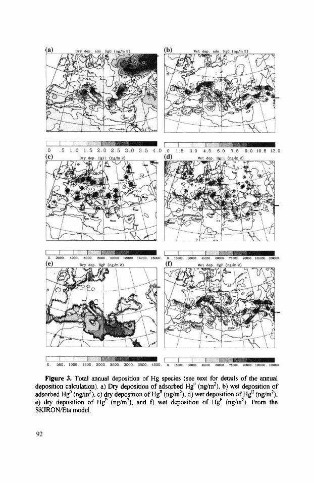
92

from Europe downstream over the Mediterranean Basin, than over land despite the factthat all anthropogenic sources are located over land. This is due to the dependence of the
great influence on deposition velocities (Sehmel, 1980).The “annual” wet deposition patterns of the three mercury species are illustrated in
Figs. 3b, d, f. The wet deposition patterns follow the rain pattern simulated by theatmospheric model. For example, this can be understood from the fact that the highest wetdeposition amounts are estimated in the vicinity of mountainous regions (e.g. Alps, Atlasmountains, Dinaric Alps).
The seasonal and “annual” depositions averaged in the entire model domain arepresented in Table 1. The wet depositions of and are in general one order ofmagnitude larger than the dry deposition ones (Table 1) contradictory to the calculatedvalues of the dry-wet deposition of that are almost the same.
Some of the similarities and differences between conventional air pollution modelingand mercury modeling have been examined in this study. The main differences aredetected in the temporal and spatial scales of various physicochemical processes involvedin the mercury cycle in the atmosphere. These processes are varying according to mercuryspecies. is considered as long-range transport pollutant, is fast reacting anddeposits quickly (wet and dry) while has behaviour similar to the other particulate inthe atmosphere. Thus mercury can be considered both long and short-range transportpollutant. The results of this study showed that the Mediterranean Sea region is not onlyaffected by mercury released in its vicinity but also from air masses enriched in mercuryfrom stations in northern and North-eastern Europe. This suggests that local and remoteemissions must be taken into account in mercury studies in the Mediterranean.
The deposition patterns of mercury exhibited several similarities with depositionpatterns estimated in previous work for other conventional air pollutants. During thesummer period, the Mediterranean Sea Region is characterised by anticyclonic
93
In general the deposition patterns show that large amounts of mercury are deposited inthe Mediterranean region.
4. CONCLUSIONS
deposition velocity of on the size of the particles. Particle diameter is known to have a

Electric Power Research Institute technical report TR-107695, 1996: Mercury in the environment-A researchupdate. Final report, EPRI, Palo Alto, CA.
Kallos, G., V., Kotroni, K., Lagouvardos, M., Varinou, M., Uliasz, and A., Papadopoulos 1997a: Transport andTransformation of air pollutants from Europe to East Mediterranean Region (T-TRAPEM). Final ReportAthens, Greece, pp.298
Kallos, G., S. Nickovic, A. Papadopoulos, D. Jovic, O. Kakaliagou, N. Misirlis, L. Boukas, N. Mimikou, G.Sakellaridis, J. Papageorgiou, E. Anadranistakis and M. Manousakis 1997b: The Regional weather forecastingsystem SKIRON. Proceedings of the Symposium on Regional Weather Prediction on Parallel ComputerEnvironments, 15-17 October 1997, Athens, Greece. 109-122.
Kallos, G., V., Kotroni, K., Lagouvardos, A., Papadopoulos, M., Varinou, O., Kakaliagou, M., Luria, M., Peleg,A., Wanger, and M., Uliasz, 1998: Temporal and spatial scales for transport and transformation processes inthe eastern mediterranean Proc. of the 22st NATO/CCMS Int. Techn. Meeting on Air Pollution Modelling andIts Application, 2-6 June, Clermont-Ferrand, France.
Kallos G., Kakaliagou O., Voudouri A., Pytharoulis I., Pirrone N., Forlano L., and J. Pachyna, 2000: Modelling ofthe mercury cycle in the atmosphere. Proceedings, 24th ITM of NATO/CCMS on Air Pollution Modelling andits Application, 15-19 May 2000, Boulder, CO, USA.
Pai, P., Karamchandani, P., and Seigneur, C., 1997: Simulation of the regional atmospheric transport and fate ofmercury using a comprehensive Eulerian model. Atm. Env., 31, 2717-2732
Pielke, R. A., Cotton W. R., Walko R. L., Tremback C. J., Lyons W. A., Grasso L. D., Nicholls M E., Moran M.D., Wesley D. A., Lee T. J., and J. H. Copeland, 1992: A comprehensive meteorological modelling system -RAMS. Meteorol. Atmos. Phys., 49, 69-91.
Pirrone N., and G. J. Keeler, 1995: Numerical Modelling of Gas-Particle Partitioning of Atmospheric Mercury inUrban Areas. In Proceedings of the 1995 Annual Meeting of the American Association for Aerosol Research(AAAR), October 9-13, 1995, Pittsburgh, Pennsylvania, U.S.A.
Pirrone N., Keeler G. J., and T. M. Holsen, 1995: Dry Deposition of Trace Elements over Lake Michigan: AHybrid-Receptor Deposition Modelling Approach. Environmental Science and Technology, 29, 2112-2122.
Slinn, S. A., and W.G.N. Slinn., 1981: Modelling of Atmospheric Particulate Deposition to Natural Waters. In:Atmospheric Pollutants in Natural Waters, S.J. Eisenreich, Ed., Ann Arbor Science, Ann Arbor, MI. pp. 22-53.
Sehmel G. A., 1980, Particle and gas dry deposition: A Review. Atm. Env., 14, pp. 983-1011.Willams, R. M., 1982: A model for the dry deposition of particles to natural water surfaces. Atmos. Environ.,
1933-1938.
94
circulations, which are known to be associated with large-scale subsidence and no rain.The amounts of the and that is dry deposited during the warm experimentalperiod are higher. The wet deposition patterns during winter showed that the largestamounts of mercury are deposited in Eastern Europe and in the Mediterranean region,especially in its eastern part. The amounts of that is deposited dry and wetare small compared to the ones of and However the deposition pattern of
is a considerable quantity as it may indicate the aerosol deposition pattern.The difficulties in measuring the wet and dry deposition of mercury make the
deposition patterns estimated by the model very useful. The models are also helpful inestimating the mercury concentration due to the lack of reliable and consistent measuringmethods. A well-developed numerical model is also much cheaper than a denseobservation network that is required for high-resolution estimations of the concentrationand deposition. From this aspect the developed models should be considered as veryuseful tools for studying the mercury processes and therefore be used by policy makers.
Acknowledgements: This work was supported by the EU-funded projects MAMCS (ENV4-CT97-0593)and ADIOS (EVK3-CT-2000-00035). The authors would like to acknowledge Prof. N. Pirrore and his group, fortheir cooperation in the model development at the framework of MAMCS project
5. REFERENCES
THE AUSTRALIAN AIR QUALITY FORECASTINGSYSTEM: MODELLING OF A SEVERE SMOKE EVENT
IN MELBOURNE, AUSTRALIA
Sunhee Lee, Martin Cope, Kevin Tory, Dale Hess, and Yuk L. Ng*
1. INTRODUCTION
The Australian Air Quality Forecasting System (AAQFS) is a joint project betweenCSIRO Atmospheric Research, CSIRO Energy Technology, the Bureau of Meteorology(BoM), the EPA Victoria and the EPA of New South Wales to develop a high-resolutionair quality forecasting system. Currently, numerical air quality forecasts are issued twicedaily for two regions: the airshed of Melbourne and Geelong in Victoria (see Figure 1)and the airshed of Sydney in New South Wales. The principal AAQFS role is to issuenumerical forecasts to State EPAs in time for guidance and reference against current airquality forecasting procedures.
The AAQFS consists of five tightly coupled components: (a) the Limited AreaPrediction System (LAPS, Puri et al., 1998), one of the BoM’s operational weatherforecasting systems, is used to generate forecasts of the transport fields at 0.05° (~5 km)horizontal grid spacing; (b) a hybrid offline/online emissions inventory module (EIM, Nget al., 2000), which generates emission flux estimates for 53 chemical species fromanthropogenic, biogenic and natural sources on horizontal grids with spacing of 0.01° forurban areas and 0.05° for non-urban areas; (c) a chemical transport model (CTM; Copeet al., 1999), which generates air quality forecasts for 25 pollutants (including PM1;PM2.5; PM10; photochemical oxidants, formaldehyde, butadiene and benzene) on ahorizontal grid spacing of 0.01° for the urban areas and 0.05° for the non-urban areas.Forecasts are undertaken using the highly condensed GRS mechanism (Azzi et al., 1992),thus enabling large domains to be simulated within the forecasting window; (d) avalidation system in which observed and forecast 1-hour time series of keymeteorological variables and air quality species are compared on a daily basis using arange of graphical and statistical tools; (e) a data dissemination and archiving systemwhich consists of an AAQFS web site displaying graphical summaries of the daily
* Sunhee Lee, CSIRO Atmospheric Research, Aspendale VIC Australia, Martin Cope, CSIRO AtmosphericResearch and Energy Technology, North Ryde NSW, Kevin Tory and Dale Hess, BMRC Melbourne VICAustralia, Yuk L. Ng, Victoria EPA, Melbourne VIC Australia
Air Pollution Modeling and Its Application XV, Edited byBorrego and Schayes, Kluwer Academic/Plenum Publishers, New York, 2002 95

forecasts for use by the EPAs, a PC-based graphical display software for visualising airpollutant species, forecast and observed meteorological variables, and a platform-independent file-archiving system.
On 11-12 January 2001, Melbourne experienced the worst visibility episode sincethe Ash Wednesday bushfire and the Melbourne Dust Storm in 1983. The episode wascaused by thick smoke emitted from bushfires on King Island (some 300 km south ofMelbourne) and Winchelsea (100 km south-west of Melbourne). Smoke from theWinchelsea fire arrived immediately behind a cold front in the afternoon of 11 January;smoke from the King Island fire first arrived in the Melbourne area during the eveningand continued to cross the region throughout the following day.
This paper describes a study in which the AAQFS was used to simulate the severesmoke event of 11-12 January.
2. CHARACTERISTICS OF THE KING ISLAND AND WINCHELSEA FIRES
The King Island fire started on 3 January 2001. Over the next 7 days the fire burnt2000-3000 ha of vegetation; the fire was thought to be under control by 10 January. On11 January, a strong south-west wind came through and the fire was re-ignited and burnt4500-5000 ha of tea-tree forest, sage-land and heath-lands. The Winchelsea fire startedat 15:55 EDT (Eastern Daylight Saving Time), 11 January and was contained by 18:00
96

EDT, though smouldering continued for another two days. The area burnt was 320 ha ofgrass-land.
Figure 2 shows GMS-5 satellite images of smoke from the King Island fire at 7:32and 12:32 EDT on 10 January and 12:32 and 15:25 EDT on 11 January. During thisperiod the winds shifted from north-easterly to north-westerly, which generated a smokeplume that extended to the south-west and rotated with time to the south-east just prior tothe arrival of the frontal wind change. The fire intensified when the winds picked up asthe front approached. The south-westerly change advected the plume to the northeast andthe most recently emitted smoke began to form a plume directed to the northeast. Smokefrom the Winchelsea fire was transported to Melbourne by the cold front and arrived atthe same time as the wind changes. The Winchelsea fire was relatively small compared tothe King Island fire and the smoke from the fire was not visible in satellite images. TheKing Island smoke plume was not clearly discernable in the satellite images after 18:30EDT, because of the presence of clouds.
97

3. THE AAQFS-LAPS METEOROLOGICAL PREDICTION
A comparison of observed and modelled winds indicated that the cold front waspredicted to arrive 1-2 hours earlier than was observed to the southwest and north ofMelbourne, while for southeast of Melbourne the timing was close to coincident. Figure3(a) and 3(b) show time-series of observed and modelled wind temperature and dewpointtemperature at Laverton, west of Melbourne, and at Moorabbin, east of Melbourne,respectively (see Figure 1). The frontal arrival is shown by the drop in temperature, therise in air moisture (represented by the rise in dewpoint temperature) and the shift in winddirection. This is considered to be a good forecast since the cold front arrival isparticularly sensitive to the balance between the weak synoptic northerlies and thedevelopment of sea and bay breezes. The latter winds can enhance the frontal structure,and accelerate or stall the larger scale wind change, which further complicates the frontalforecast. In this case the model sea/bay breeze influence differed on either side of thebay.
Figure 4(a) shows the vertical profile of observed temperature and wind structureobtained from data collected by commercial aircraft as they took-off from Melbourneairport. It shows a well-mixed layer extending to 850 hPa after 8:00 EDT 11 Januarywith winds from the north-northwest. After 16:00 EDT, the wind shifted to southerly andthe temperature dropped significantly below 950 hPa, as the colder southerly flow arrivedbehind the front. A very stable layer formed between the lower-level cold air and theremaining warmer air above. This stable layer effectively put a lid on the smoke andhelped maintain the high particle concentrations by inhibiting vertical dilution. A similarvertical profile in Figure 4(b) was constructed by interpolating the gridded model data tothe flight paths. The timing of the change and depth of the cold air is in very goodagreement with the observed profile. The diagnosed PBL height is over-predicted duringthe day due to slightly cooler temperatures between 800 and 900 hPa. Other differencesare largely due to limitations of the model grid resolution.
98
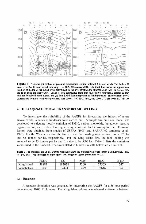
4. THE AAQFS-CHEMICAL TRANSPORT MODELLING
To investigate the suitability of the AAQFS for forecasting the impact of severesmoke events, a series of hindcasts were carried out. A simple fire emission model wasdeveloped to calculate hourly emission of PM10, carbon monoxide, butadiene, reactiveorganic carbon, and oxides of nitrogen using a constant fuel consumption rate. Emissionfactors were obtained from studies of USEPA (1995) and SAFARI-92 (Andreae et al.,1997). For the Winchelsea fire, the fire size and fuel loading were assumed to be 320 haand 5.6 tonnes per ha, respectively. For the King Island fire, the fuel loading wasassumed to be 45 tonnes per ha and fire size to be 5000 ha. Table 1 lists the emissionsvalues used in the hindcast. The times stated in hindcast results below are all in EDT.
4.1. Basecase
A basecase simulation was generated by integrating the AAQFS for a 36-hour periodcommencing 10:00 11 January. The King Island plume was released uniformly between
99

the surface and 1000 m, in accordance with visual observations. For the Winchelsea fire,emissions were uniformly placed between the surface and 500 m. Because there is someuncertainty associated with the release heights, a number of sensitivity runs wereundertaken to assess the impact on the spatial and temporal distribution of the PM10plumes (see Section 4.2).
Shown in Figure 5(a) is the ground level PM10 plume as predicted for 12:00 on 11January. At this time the plume is still within a north-westerly flow. The location of thepredicted plume is in good agreement with the observed (see Figure 2c).
Following the passage of the cold front after 17:00, both observed and modelledwinds backed from south-westerly to southerly, causing the King Island plume to rotatecounter-clockwise. The plume reached the southern edge of Port Phillip Bay at midnightand swept over Melbourne from the southeast at 2:00 12 January (Figure 5b). The easternedge of the plume had cleared Port Phillip Bay by 6:00 (Figure 5c), and had cleared theeastern metropolitan area by 7:00. However, this region was again affected by smokebetween the hours 10:00 to 11:00 inclusive. The simulation suggests that this secondimpact was caused by fumigation of PM10 from an elevated air mass, in response toconvective boundary-layer growth.
Three air quality monitoring stations in eastern Melbourne recorded PM10measurements during this smoke event. The observed PM10 measurements from thesestations showed a similar pattern; three major peaks occurred at 17:00 11 January
from midnight to 3:00, 12 January and 9:00 to 10:00, 12January The initial peak represented the Winchelsea plume and themajor peaks were from the King island plume and fumigation. The AAQFS simulation,as described above, agreed well with the observed timing of peak occurrences, however,the observed maximum concentrations of PM10 were under-predicted.
4.2. Sensitivity Studies
In order to investigate sensitivity of plume distribution and timing with respect torelease height, two sensitivity runs were carried out.
In the first run, emissions from King Island were allocated with an effective plumeheight of 1000 m. In the case of Winchelsea, the effective plume height was set to 500m.
The effect of locating all of the plume mass at these heights was seen in both thetiming and the magnitude of the PM10 impacts on Melbourne. For example, the smokeplume was now predicted to reach Port Phillip Bay at 2:00 (two hours later than thebasecase) and to sweep over Melbourne at 5:00 (three hours later than basecase). On theother hand, the fumigation event occurred two hours earlier (commencing at 9:00 insteadof 11:00) and resulted in considerably higher (by up to PM10 concentrationsas shown in figure 6(a). Figure 6(b) displays the basecase PM10 concentrations for theMelbourne grid at 11:00 12 January.
In the second sensitivity run, emissions were allocated with an effective plumeheight of 500 m for King Island and of 250 m for Winchelsea. In this run, the plumereached Port Phillip Bay at 23:00 11 January (one hour earlier than the basecase) andreached Melbourne at 2:00 12 January. It cleared eastern Melbourne then moved slightlyback eastward at 9:00 before completely clearing the Melbourne area. This run did notfeature strong fumigation.
100
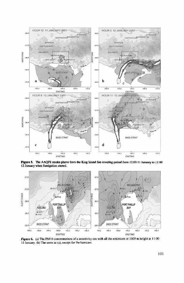
101

The impact of using different emissions factors and fire size in the simulation wasalso investigated. The resultant effects on plume distribution and magnitude wereinsignificant compared to those of using different plume release heights.
The impacts of other air quality species emitted by the wildfires, e.g.and were also modelled and found to have a reduced level of
influence compared with PM10.
5. SUMMARY
The AAQFS currently issues twice daily 24-36 hour numerical air quality forecastfor the Melbourne and Sydney regions for Victoria EPA and NSW EPA in time toprovide reference and guidance for air quality forecasting. One of the potential usages ofthe AAQFS is to provide guidance in the management of prescribed burns and in alertingthe public of smoke impacts on air quality.
On 11 January 2000, Melbourne experienced the worst visibility episode since 1983due to thick smoke from the King Island and Winchelsea bushfires. A series of theAAQFS simulations were carried out to model the severe smoke event and determine thesensitivity to emissions factors, fire size and plume height.
The AAQFS demonstrated that the modelled distribution and transport of smokeplume were qualitatively in good agreement with the observation from the satellite andmonitoring stations, with regard to the timing of plume arrival, dissipation, andfumigation. Additional tests showed that the PM10 plume development and magnitudewere sensitive to the plume release heights, while they were relatively insensitive toemissions factors and fire size.
6. ACKNOWLEDGMENT
The AAQFS was developed under funding from the Air Pollution in Major CitiesProgram, sponsored by Environment Australia.
7. REFERENCE
Andreae, A., Atlas, E., Cachier, H., Cofer, W., Harris, G., Helas, G., Koppmann, R., Lacaus, J., and Ward, D.,1977, Trace gas and aerosol emissions from savanna fires, in: Biomass Burning and Global Change Vol 1,J. Levine, ed., MIT press, Cambridge, pp. 278-295.
Azzi, M., Johnson, G. J., and Cope, M., 1992. An introduction to the Generic Reaction Set photochemica smogmechanism. Proc. 11th International Clean Air Environment Conf., 5-9 July 1992, Brisbane, Clean AirSociety of Australia and New Zealand, 451-462.
Cope, M., Hess, D., Lee, S., Azzi, M., Carras, J., Wong, N., and Young, M., 1999. Development of theAustralian Air Quality Forecasting System: Current status. Proc. International Conf. Urban Climatology,8-12 November 1999, Sydney, 595-600.
Ng, Y. L., Walsh, S. and Wong, N., 2000. Emissions model for the Australian Air Quality Forecasting System.Proc. 15th International Clean Air Environment Conf., Vol. 1, 26-30 November 2000, Sydney, Clean AirSociety of Australia and New Zealand, 275-280.
Puri, K., Dietachmayer, G., Mills, G. A., Davidson, N. E., Bowen, R. A., Logan, L. W., 1998. The new BMRCLimited Area Prediction System, LAPS. Aust. Met. Mag., 47, 203-213.
USA EPA, Compilation of air pollutant emission factors, Vol 1, Stationary point and area sources, AP-42, 1995.
102
DISCUSSION
B.J. ABIODUN
S. LEE
D. STEYN
S. LEE
A.I. MIRANDA
S. LEE
A. HANSEN
S. LEE
1) Is you meteorology model a hydrostatic or non-hydrostaticmodel ?
2) Is your dispersion using a Langrangian or a Eulerian model ?No. LAPS (Limited Area Prediction System) is hydrostatic andEulerian.
Australian bushland has plant species not found in North America.How did you find emission factors in the EPA guidelines to matchAustralian bush ?
For a grass fire, which is the case for the Winchelsea fire, PM10emission factor was obtained from U.S. EPA fire module manual.For the same reason as the question mentioned, we use PM10 factorfor the King Island fire from Andreas (1997) which was obtainedfrom SAFARI-92 experiment in the South Africa. The King Islandfire sources are tea-tree forest and heath lands. It is thought to becloser to Savanah vegetation than N. American vegetation.
Do you have any information concerning the fire behaviour ?Because, it is possible to estimate forest fires plume rise using theheat release and accordingly to the stability of the atmosphere. Thereare formulas to do that, specifically developed to forest fires.
Yes, we do use the Briggs formula for neutral and unstableconditions, which has two different formulas depending on themagnitude of heat release. For the stable condition we calculate theplume height from buoyancy flux. The details can be found in theCIT model manual.
Do you know why the PM 2.5 fraction of PM 10 for the fumigationepisode from 2100-2400 was so much lower than the other smokeepisodes ?
The fumigation period was from 9:00 am to 12:00 am. There was noobserved PM 2.5 available for the period of 10:00 – 11:00. PM 2.5curve was drawn from 9:00 to 12:00, which is misleading. At 9:00and 12:00, the ratio of PM 2.5/PM 10 was 2/3, while other smoke
103

episodes showed PM ratio of ½ ~ 2/3. All three smoke episodesshowed a similar PM 2.5/PM 10 ratio.
A. BAKLANOV
S. LEE
Are there some improvements of the urban layer parameterisations inyour NWP model for the city area or you use the same physicalparameterisations (like for “rural” areas) but with other values ofinput parameters in urban zones surface flux etc.) ?
In the NWP(LAPS) model we use the same physicalparameterisations in the urban and rural areas. We have not yetincluded a detailed urban boundary-layer parameterisation. Theeffects of the urban areas are modelled through changes to the inputparameters, such as the roughness lengths for momentum, heat andmoisture, and leaf-area index. However, we post process these fieldsover urban areas to force a near-neutral boundary layer (h/L = 1)with h=hmin_urban, where hmin_urban is a representative minimumurban boundary layer height (typically O(100 m)). u* is adjustedaccordingly. This scheme is a crude attempt to account for an urbanheat island effect.
104
PRE-PROCESSOR FOR REGIONAL-SCALE FLUXESAND MIXED-LAYER HEIGHT OVER
INHOMOGENEOUS TERRAIN
S.-E. Gryning1 and E. Batchvarova1,2
1. INTRODUCTION
The distribution of mixed-layer heights, momentum and sensible heat fluxes arecritical factors in the dilution and spread of air pollutants. In dispersion models, theindividual horizontal grid cells often enclose regions of pronounced inhomogeneities.The estimation of the regional/aggregated mixed-layer height, momentum and heat fluxesis therefore a central issue for the parameterisation used in those models.
A possible approach to evaluate regional fluxes is through a flux aggregation scheme.Point measurements are combined, in one way or another, to produce regional fluxes.Such methods has received some success for regional heat fluxes, likely because forestedge effects on the heat fluxes (temperature) are rather small as compared to fluxes overforest and grass land - at least for common patch-sizes of agricultural and forested areastypically for Europe. But for regional momentum fluxes it does not work, partly becausethe regional momentum flux of a patchy landscape of surfaces with different roughnesslength add up the local momentum fluxes in a highly non-linear way, and partly becausethe contribution to the regional momentum flux also is composed of effect by isolatedtrees, houses and sharp edges between forest and grass-land which are not necessarilysmall. Local momentum and heat fluxes traditionally are determined from mastmeasurements performed in locally homogeneous terrain, either directly by turbulencemeasurements, or by applying appropriate profile-flux relationships based on Monin-Obukhov scaling theory on measured profiles of temperature and wind. Such a networkof flux measuring stations located over patches of typical and locally homogeneousterrain is inappropriate for the determination of regional surface momentum fluxes andlarge scale mixing-heights.
1 Wind Energy Department, Risø National Laboratory, DK-4000 Roskilde, Denmark2 National Institute of Meteorology and Hydrology, Academy of Sciences, Bulgaria
Air Pollution Modeling and Its Application XV, Edited byBorrego and Schayes, Kluwer Academic/Plenum Publishers, New York, 2002 105

2. METEOROLOGICAL PRE-PROCESSOR
Here is presented a met-processor for regional fluxes of momentum and sensibleheat, and mixed-layer height. The method is simplified but reflects some of the basisphysical characteristics for meso scale fluxes. The regional momentum flux is determinedbased on blending height theory, and the regional sensible heat flux as a land use averagefor the grid cell. These fluxes are used to estimate the mixed-layer height. Theinformation that is needed to apply the met-processor can be obtained from radiosondes,tall mast or acoustic soundings profiles of wind speed, and maps of land use for the area.An estimate for the heat fluxes over the various patches of the area should also beavailable.
2.1. Regional momentum flux
Near the ground the wind changes over the various surface areas ceaselessly trying toreach balance with the underlying surface. The upward diffusion of information from thesurface features reaches a certain height before the flow encounters a new surface type.Because the size of the dominant eddies increases with height, the signature of theindividual surface features is blended efficiently at higher levels. Mason (1988)introduced a blending height as the characteristic height where the flow changes frommainly reflecting local surface characteristics, to be independent of its horizontal positionand reflecting the influence on the flow of all the various surface scales. Therefore, thehorizontal variability and imbalance of the mean flow due to surface variability hardlyreaches beyond the blending height. Above the blending height the flow reflects theregional area and is horizontally homogeneous (Mahrt, 1996). Gryning and Batchvarova(1999) discuss the vertical depth of the influence of surface variation by use of otherrelationships: internal boundary layer growth and footprint analysis. The results arecomparable in value to the blending height, but are based on different physicalapproaches.
The blending height theory in the form applied here is based on a parameterisation ofthe drag coefficients at the blending height, which is taken as a function of acharacteristic horizontal length scale of the land surface variations. Following Mason(1988) and Mahrt (1996 and 1999) a stability-dependent scale value for the blendingheight can be predicted to be:
where is the standard deviation of the vertical wind speed fluctuations and is the
characteristic length scale for the horizontal surface inhomogeneities.In order to use the method, the length scale, for the area must be known. It can
be estimated from maps of land-cover subjectively or objectively by analysis of thedistribution of the surface inhomogeneities. Having an estimate of the length scale, andassuming a value of around 0.1 it is possible to estimate the blending height for
the area.
106

When dealing with inhomogeneous conditions the regional (effective or aggregated)roughness length for momentum can be defined as the parameter that gives the correctsurface stress for the area as a whole when used in connection with a wind profilerelationship. The blending height can also be considered as the level where the wind-profile becomes independent of the horizontal position and is in equilibrium with theoverall surface conditions
where is the von Karman constant, is the effective friction velocity, is the
effective roughness length for the inhomogeneous area that will yield the correct surfacestress from the wind profile and remains to be determined from the surfacecharacteristics, is the wind profile stability correction function and is the Monin-
Obukhov length incorporating the effective momentum and sensible heat fluxes (Woodand Mason, 1991).
For a homogeneous area the drag coefficient for near neutral conditions, is
given by (Stull, 1988)
At the blending height the wind speed is nearly horizontally constant. Mason (1988)proposes that the drag coefficient at the blending height for the entire area should beestimated as the drag coefficients for the various sub areas weighted in proportion to theirfraction of the area. Therefore
where is the fraction of the total area covered by the ith surface having the local
momentum roughness length The effective roughness length, represents the
surface stress that originates from surface roughness and does not include the effect ofmajor obstacles such as topography, isolated buildings, houses and forest edges asdiscussed by Raupach (1992). Wood and Mason (1991) found that while is a function
of stability this dependence is small, and for all practical purposes can be neglected.The effective roughness length for the area can be determined by Eq. (4) from
information on land-cover and blending height. To a first approximation the stabilitydependence on in Eq. (4) can be neglected. Knowing and the regional friction
velocity, at a given time can be determined from Eq. (2) by use of the wind-speed at
107
the blending height that is known from i. e. the radiosoundings. Application of themethod when the stability correction in Eq. (2) cannot be neglected, require informationon the regional heat flux - see the next section.
2.2. Regional heat flux
For the regional heat fluxes, the so-called tile approach is considered. In order toapply this approach, the heat fluxes over the patchy sub-areas most be known as well asthe extend of the areas. The applied approach for regional heat flux estimation is aweighted average of the patch estimates of the heat fluxes in relation to the landscapeclasses:
Here represent a sub-area with heat flux A is the total area. In this
process the interaction between the subareas has been neglected. This has in a number ofstudies been found to be a reasonable assumption for patch sizes of some km or larger,which is typical for most European landscapes. For smaller patch sizes the applicabilityof the tile method has not yet been investigated.
2.3 Mixed-layer height
The upward diffusion of information on the surface features reaches a certain heightbefore the flow encounters a new surface type. With large scale inhomogeneities or ashallow mixed layer the influence of the individual surface features may extend up to thetop of the mixed layer. In this case the time averaged flow at any level within the mixedlayer will vary spatially, Mahrt, 1996, and the heat flux estimated by the methodpresented here will represent local conditions. At smaller scales of the inhomogeneities ora deeper mixed layer the level at which the individual surface features are no longer feltand the time averaged flow properties are spatially invariant is embedded within themixed layer. In this case a conventional mixed-layer growth model can be applied whenthe regional values of the parameters are used.
For example the mixed-layer growth model suggested by Batchvarova and Gryning(1991) takes the form for a patchy landscape:
where t is time, - the effective Monin-Obukhov length composed of
and g / T - the buoyancy parameter, A, B and C are parameterisation constants. Com-
108
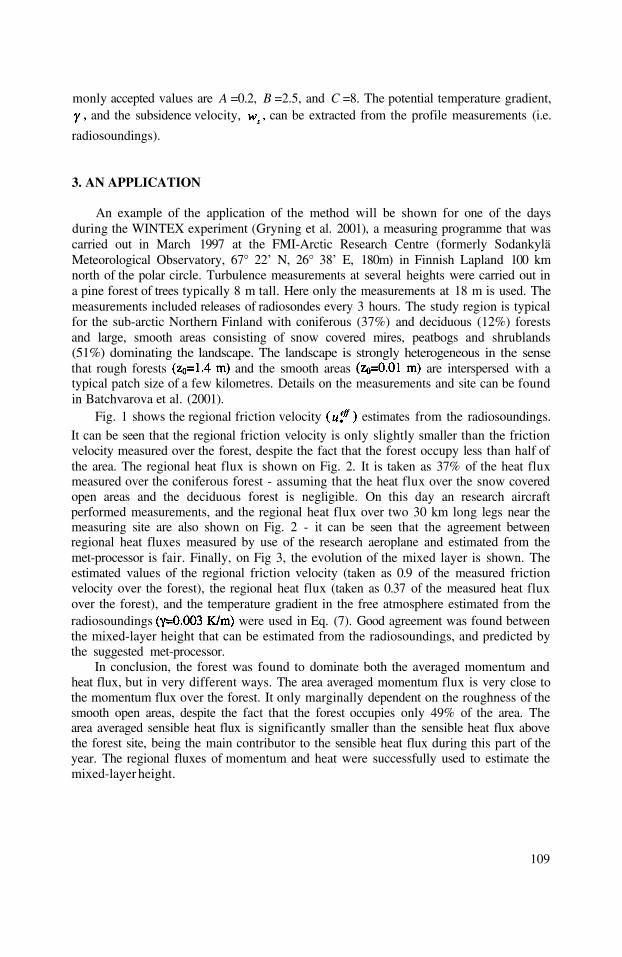
monly accepted values are A =0.2, B =2.5, and C =8. The potential temperature gradient,and the subsidence velocity, can be extracted from the profile measurements (i.e.
radiosoundings).
3. AN APPLICATION
An example of the application of the method will be shown for one of the daysduring the WINTEX experiment (Gryning et al. 2001), a measuring programme that wascarried out in March 1997 at the FMI-Arctic Research Centre (formerly SodankyläMeteorological Observatory, 67° 22’ N, 26° 38’ E, 180m) in Finnish Lapland 100 kmnorth of the polar circle. Turbulence measurements at several heights were carried out ina pine forest of trees typically 8 m tall. Here only the measurements at 18 m is used. Themeasurements included releases of radiosondes every 3 hours. The study region is typicalfor the sub-arctic Northern Finland with coniferous (37%) and deciduous (12%) forestsand large, smooth areas consisting of snow covered mires, peatbogs and shrublands(51%) dominating the landscape. The landscape is strongly heterogeneous in the sensethat rough forests and the smooth areas are interspersed with atypical patch size of a few kilometres. Details on the measurements and site can be foundin Batchvarova et al. (2001).
Fig. 1 shows the regional friction velocity estimates from the radiosoundings.It can be seen that the regional friction velocity is only slightly smaller than the frictionvelocity measured over the forest, despite the fact that the forest occupy less than half ofthe area. The regional heat flux is shown on Fig. 2. It is taken as 37% of the heat fluxmeasured over the coniferous forest - assuming that the heat flux over the snow coveredopen areas and the deciduous forest is negligible. On this day an research aircraftperformed measurements, and the regional heat flux over two 30 km long legs near themeasuring site are also shown on Fig. 2 - it can be seen that the agreement betweenregional heat fluxes measured by use of the research aeroplane and estimated from themet-processor is fair. Finally, on Fig 3, the evolution of the mixed layer is shown. Theestimated values of the regional friction velocity (taken as 0.9 of the measured frictionvelocity over the forest), the regional heat flux (taken as 0.37 of the measured heat fluxover the forest), and the temperature gradient in the free atmosphere estimated from theradiosoundings were used in Eq. (7). Good agreement was found betweenthe mixed-layer height that can be estimated from the radiosoundings, and predicted bythe suggested met-processor.
In conclusion, the forest was found to dominate both the averaged momentum andheat flux, but in very different ways. The area averaged momentum flux is very close tothe momentum flux over the forest. It only marginally dependent on the roughness of thesmooth open areas, despite the fact that the forest occupies only 49% of the area. Thearea averaged sensible heat flux is significantly smaller than the sensible heat flux abovethe forest site, being the main contributor to the sensible heat flux during this part of theyear. The regional fluxes of momentum and heat were successfully used to estimate themixed-layer height.
109
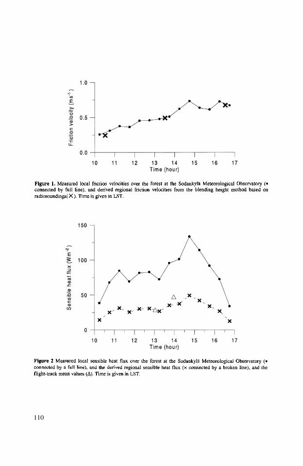
110
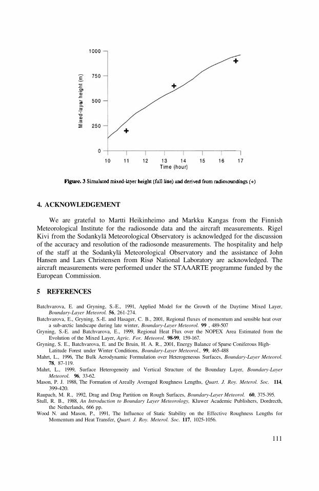
4. ACKNOWLEDGEMENT
We are grateful to Martti Heikinheimo and Markku Kangas from the FinnishMeteorological Institute for the radiosonde data and the aircraft measurements. RigelKivi from the Sodankylä Meteorological Observatory is acknowledged for the discussionof the accuracy and resolution of the radiosonde measurements. The hospitality and helpof the staff at the Sodankylä Meteorological Observatory and the assistance of JohnHansen and Lars Christensen from Risø National Laboratory are acknowledged. Theaircraft measurements were performed under the STAAARTE programme funded by theEuropean Commission.
5 REFERENCES
Batchvarova, E. and Gryning, S.-E., 1991, Applied Model for the Growth of the Daytime Mixed Layer,Boundary-Layer Meteorol. 56, 261-274.
Batchvarova, E., Gryning, S.-E. and Hasager, C. B., 2001, Regional fluxes of momentum and sensible heat overa sub-arctic landscape during late winter, Boundary-Layer Meteorol. 99 , 489-507
Gryning, S.-E. and Batchvarova, E., 1999, Regional Heat Flux over the NOPEX Area Estimated from theEvolution of the Mixed Layer, Agric. For. Meteorol. 98-99, 159-167.
Gryning, S. E., Batchvarova, E. and De Bruin, H. A. R., 2001, Energy Balance of Sparse Coniferous High-Latitude Forest under Winter Conditions, Boundary-Layer Meteorol., 99, 465-488
Mahrt, L., 1996, The Bulk Aerodynamic Formulation over Heterogeneous Surfaces, Boundary-Layer Meteorol.78, 87-119.
Mahrt, L., 1999, Surface Heterogeneity and Vertical Structure of the Boundary Layer, Boundary-LayerMeteorol. 96, 33-62.
Mason, P. J. 1988, The Formation of Areally Averaged Roughness Lengths, Quart. J. Roy. Meterol. Soc. 114,399-420.
Raupach, M. R., 1992, Drag and Drag Partition on Rough Surfaces, Boundary-Layer Meteorol. 60, 375-395.Stull, R. B., 1988, An Introduction to Boundary Layer Meteorology, Kluwer Academic Publishers, Dordrecth,
the Netherlands, 666 pp.Wood N. and Mason, P., 1991, The Influence of Static Stability on the Effective Roughness Lengths for
Momentum and Heat Transfer, Quart. J. Roy. Meterol. Soc. 117, 1025-1056.
111

DISCUSSION
S. INCECIK
E. BATCHVAROVA
A. HANSEN
E. BATCHVAROVA
M. KAASIK
E. BATCHVAROVA
112
What is the reason of the big differences in the first period ofmodeled and measured mixing layer heights ?What kind of measurement system is used for mixing layerheight ?
The different performance of the Richardson numbermethods based on HIRLAM output during the first and thesecond part of the experimental period is due to thehorizontal resolution of the present version (22.5 x 22.5 km)which does not allow to take into account the influence of theisland of Bornholm situated 20 km south west of themeasuring site. The wind during the first period of theexperiment was from south west.During the second part of the experiment the wind turned toNorth with a fetch of 100 km over sea which is welldescribed by the present version of HIRLAM.Slow (boundary-layer) radio soundings were performed tomeasure the mixed-layer height.
There are a large number of techniques for inferring mixing heightfrom observational data from rawinsondes, sodars, radar profilers,lidars, etc. Often they do not agree with one another. Whatmethod did you use to determine the mixing height based on therawinsonde data ?
The mixed-layer height was estimated from radiosondetemperature and humidity profiles. The top of the boundary layerwas assigned to the height where the potential temperature startsto increase. The humidity profile was considered simultaneously.
Can we expect in winter conditions the prevailing ascending airflow over forest and descending flow over snow surface (inpatchy landscape) ?
Yes, this forest-open land circulation can be expected.
1)
2)
1)
2)

A. BAKLANOV
E. BATCHVAROVA
I agree with you the slab model is one of the best models for CBLheight over inhomogeneous terrain. However, I think, it is not agood way to compare the model with the bulk Ri-method basedon so poor resolution NWP data. The island has almost sub-gridscale, so, of course, it is impossible to catch correctly the islandeffect on mixing height. Do you agree with this ?
Yes, thank you for the comment. The idea is to emphasise thatoutput from the HIRLAM model can be used for mixed-layerheight estimates based on Richardson number methods only whenthe upwind area can be considered as homogeneous for severalgrid steps.The study on marine boundary layer presented on the talk is notincluded in the conference manuscript. It is under publication inBLM/2001-2002: Gryning and Batchvarova, “Marine boundarylayer height and turbulent fluxes over the Baltic sea;measurements and modelling.”
113

This page intentionally left blank
VALIDATION OF URBAN AIR-QUALITYMODELLING IN THE EUROPEAN UNION
Peter Suppan1 and Andreas N. Skouloudis2
INDRODUCTION1.
During the AUTOOIL-II Programme of the European Commission (DG-ENV, 1996and 2001), a large number of air-quality modelling applications were carried out in orderto examine the attainment of the new EU Air-Quality standards for NO2, O3, CO,benzene and PM10 in the base year 1995 and forecast the concentrations in 2010. Anadvanced modelling methodology (Skouloudis and Suppan, 2000) was establishedincorporating state-of-the-art models and many innovative features (emission source-apportionment, cluster analysis for identifying the representative episodes meeting theobjectives of the this programme, two-way nesting, multi-scale simulations down tostreet-canyon levels, etc). The definition of the modelling domains was linked to thepopulation density, covering 46.7% of the European population living in urban areas atthe member states, while at the same time maintaining a consistent platform ofcomparisons with the AUTOOIL-I programme which was carried out for the base year of1990. For this a set of ten mega-city domains where defined for which urban air qualitymodelling applications were carried out (Figure 1). Apart from the objective to meet thenew threshold of NO2, also special emphasis was made to examine the consequences forother pollutants simultaneously, for which air quality standards exist (CO, Benzene andPM10). Hence, contrary to the approach from the first AUTOOIL programme, fullphotochemical simulations were carried out during at least three representative periods.
2. MODEL SETUP
Depending on the topographically complexity of the domain the meteorologicalmodelling was carried out with an incompressible, hydrostatic or a compressible, non-
1 Fraunhofer Inst. for Atmos. Env. Research, Kreuzeckbahnstr. 19, D-82467 Garmisch-Partenkirchen, Germany2 European Commission, Joint Research Centre “Ispra”, Environment Institute, T.P. 280, 21020 Ispra, Italy
Air Pollution Modeling and Its Application XV, Edited byBorrego and Schayes, Kluwer Academic/Plenum Publishers, New York, 2002 115
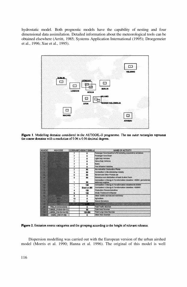
hydrostatic model. Both prognostic models have the capability of nesting and fourdimensional data assimilation. Detailed information about the meteorological tools can beobtained elsewhere (Arritt, 1985; Systems Application International (1995); Droegemeieret al., 1996; Xue et al., 1995).
Dispersion modelling was carried out with the European version of the urban airshedmodel (Morris et al. 1990; Hanna et al. 1996). The original of this model is well
116
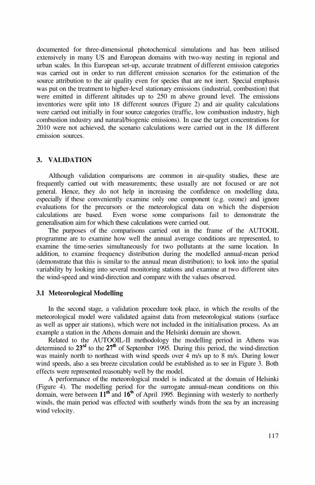
documented for three-dimensional photochemical simulations and has been utilisedextensively in many US and European domains with two-way nesting in regional andurban scales. In this European set-up, accurate treatment of different emission categorieswas carried out in order to run different emission scenarios for the estimation of thesource attribution to the air quality even for species that are not inert. Special emphasiswas put on the treatment to higher-level stationary emissions (industrial, combustion) thatwere emitted in different altitudes up to 250 m above ground level. The emissionsinventories were split into 18 different sources (Figure 2) and air quality calculationswere carried out initially in four source categories (traffic, low combustion industry, highcombustion industry and natural/biogenic emissions). In case the target concentrations for2010 were not achieved, the scenario calculations were carried out in the 18 differentemission sources.
3. VALIDATION
Although validation comparisons are common in air-quality studies, these arefrequently carried out with measurements; these usually are not focused or are notgeneral. Hence, they do not help in increasing the confidence on modelling data,especially if these conveniently examine only one component (e.g. ozone) and ignoreevaluations for the precursors or the meteorological data on which the dispersioncalculations are based. Even worse some comparisons fail to demonstrate thegeneralisation aim for which these calculations were carried out.
The purposes of the comparisons carried out in the frame of the AUTOOILprogramme are to examine how well the annual average conditions are represented, toexamine the time-series simultaneously for two pollutants at the same location. Inaddition, to examine frequency distribution during the modelled annual-mean period(demonstrate that this is similar to the annual mean distribution); to look into the spatialvariability by looking into several monitoring stations and examine at two different sitesthe wind-speed and wind-direction and compare with the values observed.
3.1 Meteorological Modelling
In the second stage, a validation procedure took place, in which the results of themeteorological model were validated against data from meteorological stations (surfaceas well as upper air stations), which were not included in the initialisation process. As anexample a station in the Athens domain and the Helsinki domain are shown.
Related to the AUTOOIL-II methodology the modelling period in Athens wasdetermined to to the of September 1995. During this period, the wind-directionwas mainly north to northeast with wind speeds over 4 m/s up to 8 m/s. During lowerwind speeds, also a sea breeze circulation could be established as to see in Figure 3. Botheffects were represented reasonably well by the model.
A performance of the meteorological model is indicated at the domain of Helsinki(Figure 4). The modelling period for the surrogate annual-mean conditions on thisdomain, were between and of April 1995. Beginning with westerly to northerlywinds, the main period was effected with southerly winds from the sea by an increasingwind velocity.
117
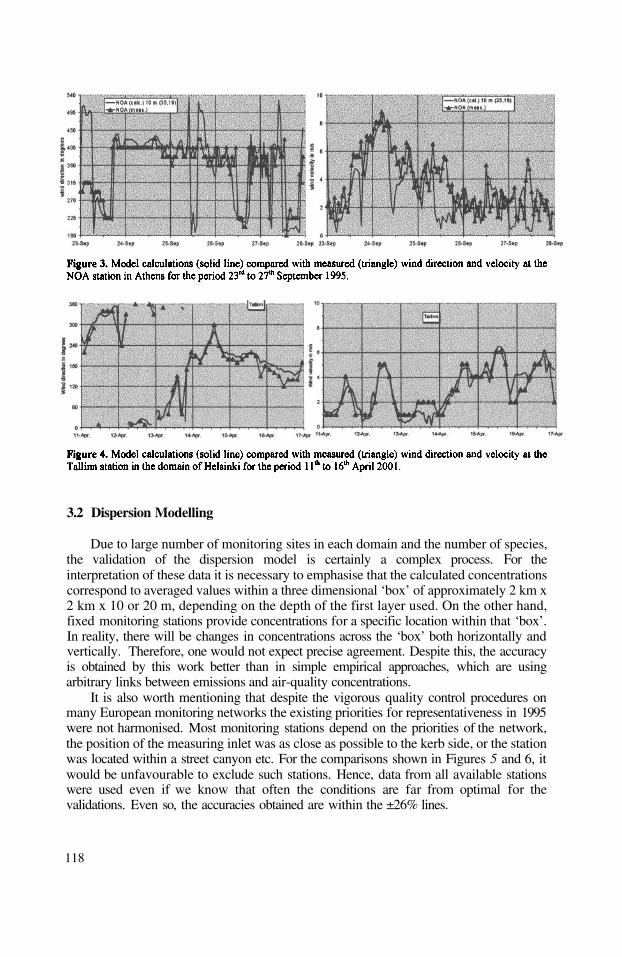
Due to large number of monitoring sites in each domain and the number of species,the validation of the dispersion model is certainly a complex process. For theinterpretation of these data it is necessary to emphasise that the calculated concentrationscorrespond to averaged values within a three dimensional ‘box’ of approximately 2 km x2 km x 10 or 20 m, depending on the depth of the first layer used. On the other hand,fixed monitoring stations provide concentrations for a specific location within that ‘box’.In reality, there will be changes in concentrations across the ‘box’ both horizontally andvertically. Therefore, one would not expect precise agreement. Despite this, the accuracyis obtained by this work better than in simple empirical approaches, which are usingarbitrary links between emissions and air-quality concentrations.
It is also worth mentioning that despite the vigorous quality control procedures onmany European monitoring networks the existing priorities for representativeness in 1995were not harmonised. Most monitoring stations depend on the priorities of the network,the position of the measuring inlet was as close as possible to the kerb side, or the stationwas located within a street canyon etc. For the comparisons shown in Figures 5 and 6, itwould be unfavourable to exclude such stations. Hence, data from all available stationswere used even if we know that often the conditions are far from optimal for thevalidations. Even so, the accuracies obtained are within the ±26% lines.
118
3.2 Dispersion Modelling

In the remaining part of this work is shown a flavour of randomly selected resultsfrom comparisons carried out in each city domain during 1995. Comparisons for otherpollutants and for other modelled episode periods can be consulted athttp://autooil.jrc.cec.eu.int.
In Figure 7 are shown comparisons for the time series for NO2 at two monitoringsites one in Lyon and one in Madrid respectively. Table 1 examines the spatial accuracyof the modelled and measured concentrations simultaneously for NO2, CO and Benzenein London. The period of the quoted data in this table are for the surrogate annual-meanconditions in 1995.
119

120

The frequency distributions of the obtained concentrations in Figure 8 show that themiddle range of concentrations is accurately represented. This is true not only betweenmeasured and modelled results but also for the complete set of annual data. This is inparticular correct in most cities both for NO2 as well as for CO.
Good temporal representativeness is achieved not only during the surrogate annual-mean period. Figure 9 shows comparisons of the ozone concentration during the 98%tileepisode and during the period representing annual mean conditions. By comparing theresults in south and central European cities it was found out that the ozone problem isquite different in the south of Europe. In the latter, high ozone concentrations can bereached even during the surrogate annual mean conditions. This is related with the actuallocation, the natural background and the regional transfer of pollutants throughatmospheric dispersion.
121
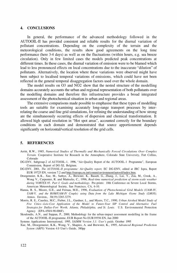
In general, the performance of the advanced methodology followed in theAUTOOIL-II has provided consistent and reliable results for the diurnal variation ofpollutant concentrations. Depending on the complexity of the terrain and themeteorological conditions, the results show good agreements on the long timeperformance (here 3-4 days) as well as on the fluctuations (within hours, e.g. sea breezecirculation). Only in few limited cases the models predicted peak concentrations atdifferent times. In these cases, the diurnal variation of emission were to be blamed whichlead to less pronounced effects on local concentrations due to the inaccurate “dilution” ofpollutants. Alternatively, the location where these variations were observed might havebeen subject to localised temporal variations of emissions, which could have not beenreflected in the general temporal disaggregation factors used over the whole domain.
The model results on O3 and NO2 show that the nested structure of the modellingdomains accurately accounts the urban and regional representation of both pollutants overthe modelling domains and therefore this infrastructure provides a broad integratedassessment of the photochemical situation in urban and regional areas.
The extensive comparisons made possible to emphasise that these types of modellingtools are suitable for examining accurately long-range transport processes by inter-relating the coarse and fine grid simulations, for refining the understanding of how strongare the simultaneously occurring effects of dispersion and chemical transformation. Itallowed high spatial resolution in “Hot spot areas”, accounted correctly for the boundaryconditions in each domain and demonstrated that source apportionment dependssignificantly on horizontal/vertical resolution of the grid cells.
Arritt, R.W., 1985, Numerical Studies of Thermally and Mechanically Forced Circulations Over ComplexTerrain. Cooperative Institute for Research in the Atmosphere, Colorado State University, Fort Collins,Colorado
DG-ENV, Subgroup-2 of AUTOOIL-1, 1996, “Air-Quality Report of the AUTOOIL-1 Programme”, EuropeanCommission, Report of DG-XI, Belgium.
DG-ENV, 2001, The AUTOOIL-II programme: Air-Quality report, EC DG-ENV, edited at JRC Ispra, ReportEUR 19725 EN, version 7.2 and http://europa.eu.int/comm/cnvironment/autooil/index.htm.
Droegemeier, K.K., Xue, M., Sathye, A., Brewster, K., Bassett, G., Zhang, J., Lui, Y., Zou, M., Crook, A.,Wong V., Carpenter, R. and Mattocks, C., 1996, Real-time numerical prediction of storm-scale weatherduring VORTEX-95. Part I: Goals and methodology. Pre-prints: 18th Conference on Severe Local Storms,American Meteorological Society, San Francisco, CA, 6-10.
Hanna, R. S., Moore, G.E., and Fernau, M.E., 1996, Evaluation of Photochemical Grid Models (UAM-IV,UAM-V, and the ROM/UAM-IV Couple) using Data from the Lake Michigan Ozone Study (LMOS).Atmos. Environ., 30(19):3265-3279.
Morris, R. E., Causley, M.C., Fieber, J.L., Gardner, L., and Myers, T.C., 1990, Urban Airshed Model Study ofFive Cities—Low-Cost Application of the Model to Future-Year SIP Control and Alternative FuelStrategies for Dallas–Fort Worth, Atlanta, Philadelphia, and St. Louis. U.S. Environmental ProtectionAgency (EPA-450/4-90-006F).
Skouloudis, A.N., and Suppan, P., 2000, Methodology for the urban-impact assessment modelling in the frameof the AUTOOIL-II programme, EUR Report No EUR19556 EN, Jan 2000
Systems Applications International, 1995, SAIMM Version 3.1: User’s guide, October 1995Xue, M., Droegemeier, K.K., Wong, V., Shapiro, A. and Brewster, K., 1995, Advanced Regional Prediction
System (ARPS) Version 4.0 User’s Guide, 380pp
122
CONCLUSIONS4.
5. REFERENCES

DISCUSSION
S. RAFAILIDIS Before using the field data for validation, did you “correct” them toaccount for local effects ? In the urban environment we know thereare large gradients present.
No, for the validation procedure we have considered only stationswhich present more than the local effects (e.g. kerb side; streetcanyons etc.). We know about the local effects and we know thatmany stations were installed for the purpose of the local air qualityand not for the purpose of modelling comparisons.
P. SUPPAN
123

This page intentionally left blank

DEVELOPMENT AND APPLICATION OF CHEMICALWEATHER FORECASTING SYSTEM OVER EAST ASIA
Itsushi Uno, Koji Ishihara, Zifa Wang, Gregory R. Carmichael and Marina Baldi *
INTRODUCTION1.
Spring dust episode (Yellow Sand or Kosa) contributes to a number ofenvironmental effects, including visibility impairment, mineral deposition, andenhancement of the pH of precipitation. Origin of yellow sand locates at the inland desertarea (such as Gobi and Takla Makan) of Asian continent. It is transported more thanseveral thousand kilometers to Japan due the springtime strong westerly. Transboundarytransport of anthropogenic air pollutants is another significant environmental problem inEast Asia because of very rapid increase of pollutants emissions due to fast economicgrowth. Anthropogenic aerosols and natural mineral dusts have a long residence time ofmore than a week and have a strong radiative forcing. Intercontinental and/or Trans-Pacific pollutant transport becomes also another important environmental issue (e.g., Unoet al, 2001b).
ACE-Asia (Asian Pacific Regional Aerosol Characterization Experiment), IGACcore research project, was designed to increase our understanding of how atmosphericaerosol particles affect the Earth’s climate system. The intensive observation was carriedout during March to May, 2001 participated using aircraft, a research vessel, surfacestations and numerical models. Aerosol transport forecast modeling activities played animportant role during the ACE-Asia intensive observation period. We developed andoperated chemical transport models - RIAM-CFORS (Research Institute for AppliedMechanics, Kyushu University & University of Iowa - Chemical weather FORecastSystem) in forecast mode and participated in flight planning activities at the operationscenter of ACE-Asia in Iwakuni, Japan. In this paper we will present an overview of theRIAM-CFORS system and summarize the general aerosol transport pattern and averagedconcentration including aerosol optical depth during the March and April, 2001.
* Itsushi UNO, Research Institute for Applied Mechanics/ Kyushu Univ., Kasuga Park 6-1, Kasuga 816-8580,Japan; Zifa Wang, Itsushi UNO, Frontier Research System for Global Change, Yokohama, Japan; KojiISHIHARA , Japan Science and Technology Corporation, Tokyo, Japan; Gregory R. CARMICHAEL ,Center for Global and Regional Environ. Research, University of Iowa, Iowa City, Iowa, U.S.A; MarinaBALDI, Institute of Atmospheric Physics (IFA-CNR), Rome, Italy.
Air Pollution Modeling and Its Application XV, Edited byBorrego and Schayes, Kluwer Academic/Plenum Publishers, New York, 2002 125
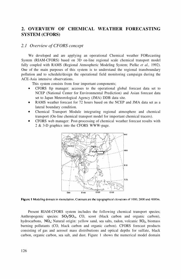
We developed and are applying an operational Chemical weather FORecastingSystem (RIAM-CFORS) based on 3D on-line regional scale chemical transport modelfully coupled with RAMS (Regional Atmospheric Modeling System; Pielke et al., 1992).One of the main purposes of this system is to understand the regional transboundarypollution and to schedule/design the operational field monitoring campaign during theACE-Asia intensive observations.
This system consists from four important components;CFORS ftp manager: accesses to the operational global forecast data set toNCEP (National Center for Environmental Prediction) and Asian forecast dataset to Japan Meteorological Agency (JMA) DDB data site.RAMS weather forecast for 72 hours based on the NCEP and JMA data set as alateral boundary condition.Chemical Transport Module integrating regional atmosphere and chemicaltransport (On-line chemical transport model for important chemical tracers).CFORS web manager: Post-processing of chemical weather forecast results with2 & 3-D graphics into the CFORS WWW-page.
Present RIAM-CFORS system includes the following chemical transport species;Anthropogenic species: CO, scoot (black carbon and organic carbon),hydrocarbons, Natural origin: yellow sand, sea salts, radon, volcanic biomassburning pollutants (CO, black carbon and organic carbon). CFORS forecast productsconsisting of gas and aerosol mass distributions and optical depths for sulfate, blackcarbon, organic carbon, sea salt, and dust. Figure 1 shows the numerical model domain
126
2. OVERVIEW OF CHEMICAL WEATHER FORECASTINGSYSTEM (CFORS)
Overview of CFORS concept2.1

which centered at 25N 115E. The horizontal grid consists of 100 by 90 grid points, with aresolution of 80 km. In the vertical, the domain is divided into 23 layers (top level is20km). These model domain configuration is capable to forecasting the most of importantchemical environment in Asia.
RIAM-CFORS tracer model is fully coupled with RAMS, and this is a uniqueapproach because the regional meteorological conditions such as precipitation, cloudmicrophysics, diurnal cycle of boundary-layer turbulence play significant role in the wetdeposition and vertical diffusion of tracers. The on-line tracer model runs with same timestep as the RAMS, so that all the on-line meteorological information such as 3-D windfield, boundary-layer turbulence, surface fluxes and precipitation amount is directly usedby the tracer model at every time step. Therefore RAMS plays the core part of CFORS tosimulate the regional scale 3-D meteorological field. General description of RAMS andits capabilities are given in Pielke et al. (1992).
2.2 Meteorological Data setRIAM-CFORS can be operated both in forecasting and hindcasting modes. During
the ACE-Asia operation, RIAM-CFORS was operationally used in forecasting mode andprovided regional forecasts of meteorology and gas/aerosol distribution using a limitedarea transport model coupled with RAMS initialized by NCEP (National Center forEnvironmental Prediction/ NOAA) and JMA (Japan Meteorological Agency) forecastproducts from their web page.
After the field campaign, we applied the RIAM-CFORS with the hindcast modebetween February 20, 2001 and May 31, 2001 by the updated boundary conditions. Inthis hindcast (post analysis) study, we used the ECMWF global meteorological data set (6hour interval with 1 deg resolution), analyzed weekly SST(sea surface temperature) dataand observed monthly snowcover information as the boundary condition of RAMScalculation.
2.3 Emission Data setAll the anthropogenic emission inventories CO, Black Carbon, Organic
Carbon and Hydrocarbons) are taken from the work of Streets (2001). It consisted withthe year 2000-based grided annual emission (1 deg resolution). Particulate matteremission from household sector is important to simulate the general background level of
and aerosol, however because of the lack of such emission data base, we didnot include it in the present study.
Natural gas/aerosol sources are assigned by using the information taken from RAMSmeteorological field and land use category information.
Identification of natural dust source region is a key issue of dust simulation, butusually detailed source information is difficult to obtain. In this study, natural dustemission area is defined as the area where USGS vegetation type (based on AVHRR dataobtained in 1992/93) is assigned as desert or semi-desert. By using this method, most partof Gobi and Takla Makan Desert are indexed as source regions. In the present calculation,Loess Plateau and Nei Mongol’s small desert (north west of the Shenyang city) area arealso assigned as the dust sources based on TOMS AI (aerosol index) observation. Most ofthe Himalayan mountain range is also indexed as desert region, but the monthly snowcover data are used to mask the undesirable dust emission from such high mountains.
127

Dusts are emitted into the atmosphere as a result of high surface winds. One majorproblem regarding long-range transport of dust is how to calculate emission rate fromsource into the atmosphere. In this work, simple vertical dust deflatation schemeproposed by Gillette and Passi (1988) is used and 12 dust particles bin (ranged from 0.1to in diameter) are assigned in the model.
Another important aerosol sources in the springtime Asia are biomass burning originCO and scoot (black carbon BC and organic carbon OC). These emission rate are highlyuncertain and changes day by day. In this present calculation, we assigned the monthlyaveraged CO, BC and OC emission estimates analyzed from AVHRR and World Firecount in the springtime of the year 2000 (Woo and Streets, 2001). This monthly averagedemission are used through out the simulation period. For example, the total biomassburning CO emission intensity exceeded the one from the anthropogenic activity withinthe modeling domain.
Sea salt also plays an important role for radiative transfer. We simulated sea saltemission and transport process with two bin modes within CFORS framework. Sea saltemission are calculated after Gong et al.(1997).
Lighting is also important as the precursors and is assigned by the subgridscale cumulus activity calculated by simplified Kuo cumulus scheme. Lightning areemitted between cloud base and cloud top as the function of cloud top height when itexists. As the volcano emission gas tracer, estimated emission intensity are used atthe major active volcanoes within the modeling domain. As the land surface origin airmass tracer, radon emission was assumed by the intercomparion experiments conditionspecified by Jacob et al. (1997).
Chemical reactions are all assumed to be linear reaction. Chemical conversion rate of1%/hour is assumed from to aerosol sulfate formation. Dry and wet depositionprocesses are treated based on the appropriate reference values and gravitational settlingare included into mineral dust and sea salt transport.
128
2.4 Aerosol optical depth and extinction coefficientAerosol optical depths for sulfate, black carbon, organic carbon, sea salt, dust and
total value are calculated at 500 nm after Takemura et al. (2000). Aerosol extinctioncoefficient and single scattering albedo (SSA) are also calculated to compare the Lidarobservation and satellite remote sensing data.
2.5 RIAM-CFORS daily operational cycleChemical weather forecast calculation (in forecasting mode) required huge computer
resources. Forecasting work adopts the PC parallel cluster system (Beowulf type 17nodes Linux cluster; Pentium III 600MHz) to simulate the regional scale 3-Dmeteorological/ chemical fields. With this hardware configuration, 3 days forecast can beachieved within 4 hours including post analysis.
Figure 2 shows the RIAM-CFORS daily operational cycle. All the meteorologicaland chemical forecasting calculation (two sets of model calculation based on NCEP andJMA) were conducted in the midnight and then WWW base forecasting information canbe ready by the 800 JST.

Weather pattern is one of the very important factors for the understanding of Asianscale transport of trace gas and aerosols. Previous studies (e.g., Uno et al., 1998; 2001a)pointed out that variations of wind pattern associated with changes of synoptic pressuresystem play a key role in the transport from Asia mainland to downwind countries in EastAsia.
From the middle of November to early March (winter in Japan), strong pressuregradients between Siberia (Continental) High and Okhotsk Low exists in average, whichfollows the strong winter monsoon in the region. This typical winter monsoon usuallylasts a few days, and after this, low pressure system develops and moves from Chinacontinent to eastside of Japan as a transition of weather change. Such a transition patternis usually observed 1 – 2 times per week, and this transition triggers intermittent largescale outbreak of pollutant from Asian continent.
In spring season (typically from middle of March to May in Japan), its weatherpattern is mainly characterized by a large scale traveling high/low pressure system,moving slowly eastward over the Japan main island. However, the exact separation bysuch a weather pattern is difficult. Weather pattern in March and April belongssometimes in winter mode and/or spring mode. Such a weather pattern alternation isextremely important for large scale dust storm transport and transboundary acidicpollutants outbreak in east Asia in spring.
Figure 3 shows the Air Pollution Index (API) measured for Beijing and Qingdao,China. An air pollution index is derived for each of and TSP (Total suspendedparticulates), based on a scale from 0-500 defined by the State Environmental ProtectionAgency (SEPA) of China. This figure shows the API value of TSP. API (TSP) value of500 corresponds to the TSP concentration of Solid lines in the figure shows themodel predicted dust concentration.
129
3. RESULTS AND DISCUSSION
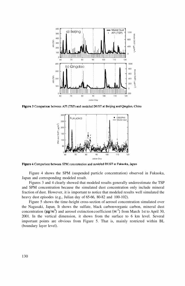
Figure 4 shows the SPM (suspended particle concentration) observed in Fukuoka,Japan and corresponding modeled result.
Figures 3 and 4 clearly showed that modeled results generally underestimate the TSPand SPM concentration because the simulated dust concentration only include mineralfraction of dust. However, it is important to notice that modeled results well simulated theheavy dust episodes (e.g., Julian day of 65-66, 80-82 and 100-102).
Figure 5 shows the time-height cross-section of aerosol concentration simulated overthe Nagasaki, Japan. It shows the sulfate, black carbon+organic carbon, mineral dustconcentration and aerosol extinction coefficient from March 1st to April 30,2001. In the vertical dimension, it shows from the surface to 6 km level. Severalimportant points are obvious from Figure 5. That is, mainly restricted within BL(boundary layer level).
130

Time variation between mineral dust and sulfate has a strong correlation. Very highconcentration is observed intermittently.Mineral dust transport height depends on the meteorological condition.Carbonaceous concentration (Black Carbon + Organic Carbon) has two layerstructures, i.e., transported within BL and above the BL, independently (verticallevel from 2000 m to 4000m in the free atmosphere).Figure 6 shows the horizontal distribution of AOD (aerosol optical depth) from
mineral dust and sulfate between March 19 and March 22, 2001. Vector in figureindicates the wind flow at the height of This period is chosen because RIAM-CFORS results and surface observation both show the very high concentration ofaerosols (Figures 3, 4 and 5). The figure clearly indicated that the sulfate and mineraldust transport to Japan area. It is interesting that the high concentration center of mineraldust and sulfate are separated (e.g., over the mainland China), however, theconcentration contour are mixed when it is transported to the Japan Sea and Japanmainland area.
Figure 7 shows the monthly averaged aerosol optical depth (AOD) from mineral dust,sulfate and carbonaceous aerosol and the total AOD from these components + sea salts inApril, 2001. This monthly averaged information provides us many interesting phenomenawhich should be compared with observations. Important information can be summarizedas follows;
131
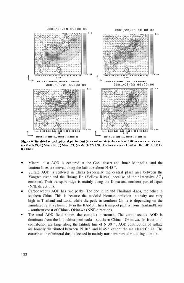
Mineral dust AOD is centered at the Gobi desert and Inner Mongolia, and thecontour lines are moved along the latitude about N 45 °.Sulfate AOD is centered in China (especially the central plain area between theYangtze river and the Huang He (Yellow River) because of their intensiveemission). Their transport ridge is mainly along the Korea and northern part of Japan(NNE direction).Carbonaceous AOD has two peaks. The one in inland Thailand -Laos, the other insouthern China. This is because the modeled biomass emission intensity are veryhigh in Thailand and Laos, while the peak in southern China is depending on thesimulated relative humidity in the RAMS. Their transport path is from Thailand/Laos- southern coast of China - Okinawa (NNE direction).The total AOD field shows the complex structure. The carbonaceous AOD isdominant from the Indochina peninsula - southern China - Okinawa. Its fractionalcontribution are large along the latitude line of N 30 ° . AOD contribution of sulfateare broadly distributed between N 30 ° and N 45 ° except the mainland China. Thecontribution of mineral dust is located in mainly northern part of modeling domain.
132
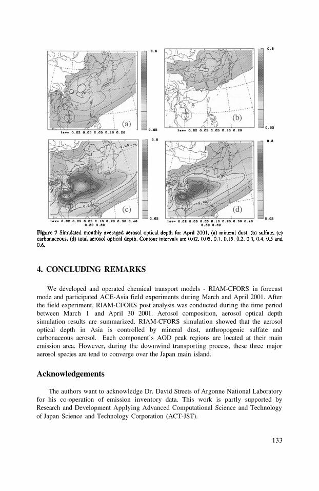
We developed and operated chemical transport models - RIAM-CFORS in forecastmode and participated ACE-Asia field experiments during March and April 2001. Afterthe field experiment, RIAM-CFORS post analysis was conducted during the time periodbetween March 1 and April 30 2001. Aerosol composition, aerosol optical depthsimulation results are summarized. RIAM-CFORS simulation showed that the aerosoloptical depth in Asia is controlled by mineral dust, anthropogenic sulfate andcarbonaceous aerosol. Each component’s AOD peak regions are located at their mainemission area. However, during the downwind transporting process, these three majoraerosol species are tend to converge over the Japan main island.
133
4. CONCLUDING REMARKS
Acknowledgements
The authors want to acknowledge Dr. David Streets of Argonne National Laboratoryfor his co-operation of emission inventory data. This work is partly supported byResearch and Development Applying Advanced Computational Science and Technologyof Japan Science and Technology Corporation (ACT-JST).

References
Gillette, D. and R., Passi, 1988, Modeling Dust Emission Caused by Wind Erosion, J. Geophy. Res., 93:14,233-14,242.
Gong, S.L., L.A., Barrie and J.-P., Blacnchet, 1997, Modeling sea-salt aerosols in the atmosphere 1. Modeldevelopment, J. Geophy. Research, 102 :3805-3818.
Jacob, D.J. et al., 1997, Evaluation and intercomparison of global atmospheric transport models using radon-222 and other short-lived tracers, J. Geophy. Research, 102:5953-5970.
Pielke, R.A., W.R.,Cotton, R.L., Walko, C.J., Tremback, W.A., Lyons, L.D., Grasso, M.E., Nicholls, M.D.,Moran, D.A., Wesley, T.J., Lee and J.H., Copeland, 1992, A comprehensive meteorological modelingsystem -RAMS, Meteorol. Atmos. Phys., 49: 69-91.
Streets, D, 2001, http://www.cgrer.uiowa.edu/ACESS/ EMISSION_DATA/ED_index.htm.Takemura, T., H., Okamoto, Y., Maruyama, A., Numaguti, A., Higurashi, and T., Nakajima, 2000, Global three-
dimensional simulation of aerosol optical thickness distribution of various origins, J. Geophy. Research,105:17,853-17,873.
Uno, I, T., Ohara and K., Murano, 1998, Simulated Acidic Aerosol Long-Range Transport and Deposition overEast Asia - Role of Synoptic Scale Weather Systems, in Air Pollution Modeling and its Application 22,S.E. Gryning and N. Chaumerliac, Ed., Plenum Pub. Co., pp. 185-193.
Uno , I., S. Emori and M. Baldi, 2001a, Chemical transport model on-line coupled with RAMS for regionalchemical climate, in Air Pollution Modeling and Its Application XIV, Gryning and Schiermeier, Ed.,Kluwer Academinc/Plenum Pub., pp. 75-85.
Uno,I., H., Amano, S., Emori, K., Kinoshita, I., Matsui and N., Sugimoto, 2001b, Trans-Pacific Yellow SandTransport observed in April 1998: Numerical Simulation, J. Geophy. Research, 106:18,331-18,344.
Woo, J.-H. and D. Streets et al., 2001, http:// www.cgrer. uiowa.edu/people/ woojh21/data_fire_ co_index.html
134

DISCUSSION
A. HANSEN
Z. WANG
P. BUILTJES
Z. WANG
One calculation you showed indicated that the carbonaceouscomponent dominated the AOD for that episode. Is this dominancethe typical case ?
Increased contribution of carbonaceous aerosols to AOD during theexperimental period is mainly due to intense biomass burning in theregion and considerably lower contribution from mineral dust. Dailyvariation in biomass burning emissions of BC and OC was estimatedusing AVHRR and TOMS AI data. For more details, please refer tohttp://www.cgrer.uiowa.edu
Did you compare computed AOD with satellite observed AOD ?
Not yet. But we are planning to compare computed AOD withsatellite observed one.
135

This page intentionally left blank
PHOTO-OXIDATION PROCESSES OVER THEEASTERN MEDITERRANEAN BASIN IN SUMMER
M. Varinou, F. Gofa, G. Kallos, M. O’Connor and G. Tsiligiridis
1. INTRODUCTION
The summertime photochemical activity over the Eastern Mediterranean Basinis examined by applying a multi-scale analysis of the atmospheric circulation. Photo-oxidation is considered to depend on both the distribution of precursor emissions and theatmospheric circulation, from the synoptic scale to the mesoscale. Characteristic spatialand temporal scales of photochemical activity are estimated using atmospheric and airquality numerical modeling in combination with experimental data. Special emphasis isgiven to the examination of the role of major coastal sources (e.g., urban areas, industrialzones) in the degradation of air quality at remote locations.
Photochemical activity over the Eastern Mediterranean has been examinedmainly on the local scale. Extensive studies have focused on the build-up processesleading to photochemical episodes in highly polluted areas, such as urban areas andindustrial zones. The most significant efforts concern the metropolitan area of Athens,Greece and the coastal area of Israel (Asimakopoulos et al., 1992; Pilinis et al., 1993;Moussiopoulos et al., 1995;Varinou, 2000). The synoptic circulation over the EasternMediterranean basin (as it is described in UKMO, 1962; Varinou, 2000 and referencesthere in) favors transport of air masses from the Western and Central Mediterranean andSE Europe towards the eastern part of the basin, the North African coast and the MiddleEast (Dayan, 1986; Katsoulis and Whelpdale, 1993). Evidence of long-range transport ofair pollutants towards the Middle East was identified by Peleg et al. (1994) and Wagneret al., (2000). Both groups found that the Israeli coastal area was a receptor of secondarypollution. Kallos et al. (1996, 1999) suggested possible transport mechanisms from majorcoastal sources on the Greek peninsula towards Africa and the Middle East duringsummer, based on numerical simulations of the atmospheric circulation and dispersion,while Kotroni et al. (1998) studied the Athens plume as it disperses downwind. The areasover the Aegean Sea and the island of Crete were identified as the main transport routes.The regional scale photochemical activity was studied during the T-TRAPEMexperimental campaign (Kallos et al., 1997; 1998)
The present study is focused on the investigation of photochemical processes inthe greater Aegean area. The behavior of the urban plume of the Greater Athens Area
*F. Gofa, G. Kallos, M. O’Connor , Dept. of Physics, University of Athens, Athens, Greece. G. TsiligiridisDept. of Mechanical Engineering, University of Thessaloniki, Thessaloniki, Greece. M. Varinou, Dept. ofPhysics, University of Athens, Athens, Greece, also, General Secretariat of Civil protection, Ministry of of theinterior public administration and decentralization.
Air Pollution Modeling and Its Application XV, Edited byBorrego and Schayes, Kluwer Academic/Plenum Publishers, New York, 2002 137

(GAA) is examined as a representative case of coastal urban photochemical pollution.The GAA acts as a large area source of precursors (due to urban and industrial activities)that possibly contributes to the photochemical degradation of air quality in remote areas.The proposed multi-scale (local to regional) analysis is based on numerical simulationswith the Regional Atmospheric Modeling System (RAMS) (Pielke et al., 1992), theCAMx (Comprehensive Air quality Model with extensions) air quality model (Environ,1997) and the Mesoscale Dispersion Modeling System (MDMS) (Uliasz, 1993). Thesimulations were designed in order to analyze the experimental evidence of regional scalephoto-oxidation of urban plumes provided by the airborne measurements performedduring the T-TRAPEM project (Kallos, 1997). This work is being continued in theframework of the EU funded projects SUB-AERO and ADIOS.
1.2. Experimental period
The simulation period extended from July 1 to 6, 1995. Experimental data fromthe T-TRAPEM campaign (Kallos et al., 1997) was available for this period. These datacomprise airborne measurements in the marine boundary layer (~1000 ft) over theCentral and Southern Aegean Sea and include (TEII 43S), NOx, TSP andVolatile Organic Compounds (VOCs) concentrations. Oxidant measurements over thegreater maritime area of the island of Crete were used in order to validate the CAMxmodel results. The origin of the relatively high ozone (60-70 ppbv) concentrationobserved from July 3 to 5 in the area of Crete was investigated by applying the MDMS.
The meteorological conditions during the experimental period werecharacterized by the alternation of typical summer time synoptic circulation types. Thegeneral synoptic characteristics were analyzed using: the European MeteorologicalBulletin charts (at 0000 and 1200 UTC), the meteorological fields provided by theECMWF (every 6 hours) and surface-radiosonde data from the National Center ofAtmospheric Research of US (every 3 hours). From July 1 to 2 a strengthening of thesynoptic flow over the NE Mediterranean occurs as a result of the interaction between thehigh pressure ridge of the Central Mediterranean and the westward extension of theAnatolian thermal low. The wind speed reaches 12 m/s over the Aegean and 8 m/s overcoastal areas. Inland there is a strong modification of the synoptic flow by the localthermal circulations that develop over the complex terrain. During the following days thesynoptic flow gradually weakens as the subtropical ridge of the Central Mediterraneanextends eastward. Transport of warm air masses from northern Africa is evident in the700-500 hPa charts and 1000/500 hPa thickness charts. The radiosonde data over Greece(Hellinikon, Athens) show a significant warming of 10°C in the 850-600 hPa layer fromJuly 3 (1200 UTC) to July 4 (1200 UTC) and strong nocturnal thermal inversions on July4 and 5. The synoptic flow gradually weakens from July 3 to 5 and the wind field isdominated by shallow thermal mesoscale circulation.
2. MODELS AND DATA USED
2.1. Models usedThe RAMS model: The Regional Atmospheric Modeling System (RAMS) has beendeveloped at Colorado State University and the ASTER Division of the Mission Research
138
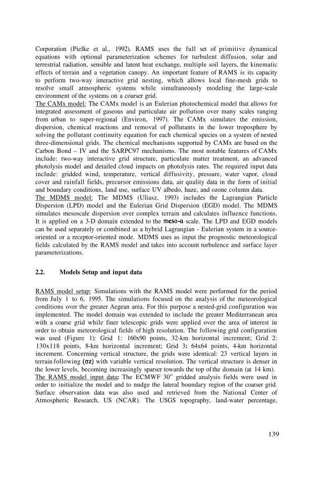
Corporation (Pielke et al., 1992). RAMS uses the full set of primitive dynamicalequations with optional parameterization schemes for turbulent diffusion, solar andterrestrial radiation, sensible and latent heat exchange, multiple soil layers, the kinematiceffects of terrain and a vegetation canopy. An important feature of RAMS is its capacityto perform two-way interactive grid nesting, which allows local fine-mesh grids toresolve small atmospheric systems while simultaneously modeling the large-scaleenvironment of the systems on a coarser grid.The CAMx model: The CAMx model is an Eulerian photochemical model that allows forintegrated assessment of gaseous and particulate air pollution over many scales rangingfrom urban to super-regional (Environ, 1997). The CAMx simulates the emission,dispersion, chemical reactions and removal of pollutants in the lower troposphere bysolving the pollutant continuity equation for each chemical species on a system of nestedthree-dimensional grids. The chemical mechanisms supported by CAMx are based on theCarbon Bond – IV and the SARPC97 mechanisms. The most notable features of CAMxinclude: two-way interactive grid structure, particulate matter treatment, an advancedphotolysis model and detailed cloud impacts on photolysis rates. The required input datainclude: gridded wind, temperature, vertical diffusivity, pressure, water vapor, cloudcover and rainfall fields, precursor emissions data, air quality data in the form of initialand boundary conditions, land use, surface UV albedo, haze, and ozone column data.The MDMS model: The MDMS (Uliasz, 1993) includes the Lagrangian ParticleDispersion (LPD) model and the Eulerian Grid Dispersion (EGD) model. The MDMSsimulates mesoscale dispersion over complex terrain and calculates influence functions.It is applied on a 3-D domain extended to the scale. The LPD and EGD modelscan be used separately or combined as a hybrid Lagrangian - Eulerian system in a source-oriented or a receptor-oriented mode. MDMS uses as input the prognostic meteorologicalfields calculated by the RAMS model and takes into account turbulence and surface layerparameterizations.
2.2. Models Setup and input data
RAMS model setup: Simulations with the RAMS model were performed for the periodfrom July 1 to 6, 1995. The simulations focused on the analysis of the meteorologicalconditions over the greater Aegean area. For this purpose a nested-grid configuration wasimplemented. The model domain was extended to include the greater Mediterranean areawith a coarse grid while finer telescopic grids were applied over the area of interest inorder to obtain meteorological fields of high resolution. The following grid configurationwas used (Figure 1): Grid 1: 160x90 points, 32-km horizontal increment; Grid 2:130x118 points, 8-km horizontal increment; Grid 3: 64x64 points, 4-km horizontalincrement. Concerning vertical structure, the grids were identical: 23 vertical layers interrain following with variable vertical resolution. The vertical structure is denser inthe lower levels, becoming increasingly sparser towards the top of the domain (at 14 km).The RAMS model input data: The ECMWF 30” gridded analysis fields were used inorder to initialize the model and to nudge the lateral boundary region of the coarser grid.Surface observation data was also used and retrieved from the National Center ofAtmospheric Research, US (NCAR). The USGS topography, land-water percentage,
139

vegetation and soil type gridded data with 30” (~1 km) resolution and the ECMWF seasurface temperature (SST) gridded data with resolution of 1° (~ 100 km) were also used.CAMx set up and input data: Simulations with the CAMx model were performed for theperiod from July 1 to 6, 1995. The CAMx simulations focused on the analysis of photo-oxidation over the greater Aegean area. For this purpose a nested-grid configuration wasimplemented (Figure 1) with two grids. The following grid configuration was used: Grid1: 143x128 points, 0.226°x0.18° horizontal increment; Grid 2: 227x257 points,0.045°x0.036° horizontal increment (SW corner at 19.7°E, 32.8°N). The vertical structurewas identical for both grids: 7 vertical layers defined in terrain followingcoordinates. Variable vertical resolution was applied with a denser vertical structure inthe lower levels, becoming increasingly sparser towards the top of the domain (at 4km).
CAMx input data: The required meteorological datasets were supplied by the RAMSprognostic meteorological fields. The gridded land use data used in RAMS were adjustedaccordingly for the CAMx grids. The Total Ozone Column for the area of interest wasretrieved from the NASA/Goddard Space Flight Center database and derives from theMeteor3/TOMS dataset. With respect to precursor emissions, the following data setswere adjusted to the CAMx grids and used in the simulations:1. An anthropogenic surface emissions inventory for Europe was retrieved from EMEP
(Co-operative program for monitoring and evaluation of the long range transmissionof air pollutants in Europe) for the year 1996. These data are in gridded form with50x50 km grid increment and include annual surface emission rates (tn/y) ofNOx, VOCs (Volatile Organic Compounds) and The VOC speciation anddiurnal emissions profile calculations were based on the factors proposed by Zlatevet. al. (1992).The surface emissions inventory for Greece was provided by Tsiligiridis (1995). Thisinventory is based on the CORINAIR methodology (CORINAIR, 1992) concerningthe types of sources and procedures, the kinds of emitted pollutants and the emissionrates. The included air pollutants are: NOx, NMVOCs (Non Methane VOCs) and
2.
140

CO. The activities contributing to these emissions include: energy import, energyconversions, energy consumption in the industrial, transport, commercial anddomestic sectors, etc. The main types of energy included are: carbon, lignite, naturalgas, gas, biomass, oil, diesel and various others. The use of solvents in industrialactivities was also taken into account. This latter category was analyzed specificallyfor this study in an 8x8 km grid, while the other types of emissions were analyzed ina 20x20 km grid.
MDMS setup and input data: Simulations with the MDMS model were performed for theexperimental periods mentioned above. The MDMS simulations focused on thecalculation of influence functions over the greater Aegean area. For this purpose areceptor area with dimensions 10km x 10km x 1km was defined at selected sitesindicated by the airborne measurements. The requisite meteorological datasets weresupplied by the RAMS prognostic meteorological fields.
3. MODELS RESULTS AND DISCUSSION
The RAMS-CAMx system simulations showed that the GAA plume maintainsmost of its characteristics over long distances (several hundreds of kilometers) above theAegean Sea due to poor mixing in the marine boundary layer or in the free atmosphere.Figures 2 and 3 present the calculated ozone concentration in the layer 250-500m abovesurface on July 3 and 4. During nighttime, the precursor pollutants emitted in the GAAare transported to the south/southeast over the maritime area of the Saronic Gulf, owingto the weak NW land breeze flow. During the day, the northerly regional scale flow overthe Aegean transports the plume further to the south. The calculated ozone concentrationsat 1200 UTC and 1500 UTC on July 3 (Figure 2) reach approximately 60ppbv over thesouthern Aegean Sea. As evident in Figures 2a and 2b, the plume reaches Crete on a timescale of about 6h. These values are close to the concentrations measured during theT_TRAPEM project (presented in Figure 5.2.36b of Kallos et al., 1997), which reach 60–70ppbv. As shown in Figure 2, the RAMS-CAMx results give evidence of regional scaletransport from the coastal area of NW Turkey towards the Aegean Sea. The situationchanges slightly the following day (July 4) as the northerly flow over the Aegeanweakens. The GAA urban plume is transported to the SE of GAA during the night andremains halfway between the GAA and Crete for more than 6h. The model results showconcentrations of about 55-60ppbv with a maximum at 65ppbv (see Figure 3). Theairborne measurements of concentrations in this area reach 60-70ppbv (Figure5.2.36e, Kallos et al., 1997). The GAA plume reaches Crete on a time scale of 12h.
The influence of the GAA urban plume on remote areas was further investigatedby calculating influence functions with the MDMS. Moreover, influence functioncalculations were used in order to identify the source areas of the photochemicalpollution measured over the greater maritime area of Crete. Simulations were performedfor various receptor areas around Crete. Figures 4 and 5 present the results from thefollowing cases: 1. Influence functions calculated for 88h backward in time, the receptorarea (A3) centered at 36.3° N, 23.4° E. Simulation started at 1600 UTC, July 3, 1995. 2.Influence functions calculated for 130h backward in time, the receptor area (A4) centeredat 35°N, 26.5°E. Simulation started at 1000 UTC, July 5, 1995.
141

The MDMS simulations confirmed the results of previous studies concerning theidentification of the main transport routes in the Eastern Mediterranean (Kallos et al.,1996; 1998; Varinou, 2000). As evident in Figures 4 and 5, the maritime area to the NWof Crete is influenced by remote pollution sources located on the Greek peninsula, over atimescale of 24h. Sources located to the NE of Greece influence this area on timescale of36h. The same timescale is identified for sources located in SE Italy. As shown by theCAMx model simulations, the GAA plume affects the receptor area after 12h. Accordingto the results from Case 2, the maritime area to the SE of Crete is influenced by pollutionsources located in the Southern Greece and Italy. The GAA influence on the receptor areaoccurs over a timescale of 18h. This result is also evident in the CAMx modelsimulations.
142

4. CONCLUSIONS
In the present study, multi-scale analysis of the atmospheric circulation andphotochemical processes was performed in order to investigate the behavior ofphotochemical plumes emitted from urban coastal areas. The simulations were combinedwith regional scale marine boundary layer airborne measurements of the atmosphericoxidants. The results showed a strong interaction between local and regional scalefluctuations. The previously identified main routes of transport were confirmed as routesof photochemical fluctuations. The key factor is the marine boundary layer. The plume
143

maintains its characteristics inside this stable layer and the diurnal fluctuation of NOy inassociation with precursor VOCs define oxidant concentration at remote areas.
Acknowledgements: This study was supported by the research projects T-TRAPEM (EV*-CT92-0005), SUB-AERO (EVK2-1999-00052) and ADIOS (EVK3-CT-2000- 00035) of the DG-XII of the EU.
REFERENCES
Asimakopoulos, D., D., Deligiorgi, C., Drakopoulos, C., Helmis, K., Kokkori, D., Lalas, D., Sikiotis, and C.,Varotsos, 1992: An experimental study of nighttime air-pollutant transport over complex terrain inAthens. Atmospheric Environment, Vol. 26B, 59-71.
CORINAIR Inventory, Default Emission Factors Handbook, Default emission factors from nature, Part 2, 1992.Dayan, U., 1986: Climatology of back trajectories from Israel based synoptic analysis. J. of Climate and
Applied Meteorology, 25, 591 - 595.Environ, 1997: User’s Guide to the comprehensive air quality model with extensions (CAMx). Version 1.10.
Report prepared by Environ International Corporation, Novato, CA.Kallos, G., V., Kotroni, K., Lagouvardos, M., Varinou, and A., Papadopoulos, 1996: Possible mechanisms for
long range transport in the eastern Mediterranean. Proc. of the 21st NATO/CCMS Int. Techn. Meetingon Air Pollution Modelling and Its Application, 6-10 November, Baltimore, USA.
Kallos G., K., Lagouvardos, V., Kotroni, A., Papadopoulos, M., Varinou, M., Luria, M., Peleg, A., Wagner, G.,Sharf, and G., Tunsel, 1997: “Transport and transformation of air pollutants in the Eastern MediterraneanArea”. Final Report prepared for the DG-XII of EC, AVICENNE Initiative. T-TRAPEM Project,ISBN960-8468-07-8.
Kallos, G , V., Kotroni, K., Lagouvardos, A., Papadopoulos, M., Varinou, O., Kakaliagou, M., Luria, M., Peleg,A., Wagner and M., Uliasz, 1998: Temporal and spatial scales for transport and transformation processesin the eastern Mediterranean Proc. of the 22nd NATO/CCMS Int. Techn. Meeting on Air PollutionModelling and Its Application, 2-6 June, Clermont-Ferrand, France.
Kallos, G., V. Kotroni, K. Lagouvardos, and A. Papadopoulos, 1999: “On the transport of air pollutants fromEurope to North Africa. Geophysical Research Letters. 25, No 5, 619-622.
Katsoulis, B.D., and D.M., Whelpdale, 1993: A climatological analysis of four-day back trajectories fromAliartos, Greece. Theor. and Appl. Climatol. 47, 93 - 103.
Kotroni, V., G., Kallos, K., Lagouvardos, M., Varinou, and R, Walko, 1998: Numerical simulations of themeteorological and dispersion conditions during an air pollution episode over Athens, Greece. J. ofApplied Meteorology, Vol., 38, pp.432-447.
Moussiopoulos, N., P., Sahm, and Ch.S., Kessler, 1995: Numerical simulation of photochemical smogformation in Athens, Greece-a case study. Atmospheric Environment, 29, No 24, pp. 3619-3632.
Peleg M., M., Luria, I., Setter, D., Perner, and P., Russel, 1994: Ozone levels over Central Israel. Isr. J. ofChemistry, 34, 375-386.
Pielke, R.A., W.R, Cotton, R. L., Walko, C. J., Tremback, W. A., Lyons, L.D., Grasso, M. E., Nicholls, M. D.,Moran, D. A., Wesley, T. J., Lee, and J. H., Copeland, 1992: A comprehensive meteorological modellingsystem - RAMS. Meteorology and Atmospheric Physics, 49, 69-91.
Pilinis, C., P., Kassomenos, and G., Kallos, 1993: Modeling of photochemical pollution in Athens, Greece.Application of the RAMS-CALGRID modeling system. Atmospheric Environment. 27B, No 4, 353-370.
Tsiligiridis, G., 1995: Temporal and spatial analysis of energy consumption and the associated emissions of airpollutants during the period 1960-’90 in Greece. PhD thesis, Dept. of Mechanical Engineering, Universityof Thessaloniki, Thessaloniki, Greece.
Uliasz, M., 1993: The Atmospheric Mesoscale Dispersion Modeling System. J. of Applied Meteorology, 32, pp.139-149.
UKMO (United Kingdom Meteorological Office), 1962: Weather in the Mediterranean, Vol. I, GeneralMeteorology, 375 pp., H.M. Stationary Office, London, Second Edition.
Varinou, M., 2000: Characteristic spatial and temporal scale of dispersion and photochemical transformations ofair pollutants over the NE Mediterranean. PhD thesis, Dept. of Physics, University of Athens, Athens,Greece, pp 300.
Wagner, A., M. Peleg, G. Sharf, Y. Mahrer, U. Dayan, G. Kallos, V. Kotroni, K. Lagouvardos, M. Varinou, A.Papadopoulos, 2000. “Some observational and Modeling evidence of long-range transport of airpollutants from Europe toward Israeli coast”. J. Geophysical Res., 105, No.D6, 7177-7186.
Zlatev, Z., J., Christensen, and O., Hov, 1992: A Eulerian air pollution model for Europe with non-linearchemistry. J. of Atmospheric Chemistry, Vol.15, pp.1-37.
144

DISCUSSION
A. EBEL
M. VARINOU
Has the role of vertical transport of pollutants, particularly ozone,also been studied for the Mediterranean region ?
The role of vertical transport of pollutants over the NEMediterranean has been extensively studied with airborneobservations and model simulations. The simulations wereperformed using RAMS and HYPACT, which is a Lagrangian-typedispersion model. Releases from major coastal urban areas such asthe Greater Athens Area were performed for various time periodsduring the day. The results showed that in the case of weak synopticflow, dispersion patterns over the Aegean are mainly affected by therelease time and the mixing height variability due to the complexland-water distribution. The pollutants released during the night andearly in the morning are transported downwards within the marineboundary layer. The modification of the mixing height due to thepresence of islands, leads to a considerable intrusion and transportabove the marine boundary layer of about 1km. The pollutantsreleased during the day are injected in the free troposphere as soonas they are released. This is attributed to the convergence over roughtopography, affecting a layer of 2-4km depth. Vertical mixingbetween this layer and the surface layer is also evident over theAegean as a result of convergence over the islands. In the case ofstrong synoptic flow no significant convergence was found over theland while the pollutants are mainly within a well-mixed layer ofabout 2km depth.
145

This page intentionally left blank

NUMERICAL STUDY OF TROPOSPHERIC OZONE INTHE SPRINGTIME IN EAST ASIA
Meigen Zhang, Itsushi Uno, Zifa Wang, and Hajime Akimoto*
1. INTRODUCTION
East Asia is a region of the world with large and rapidly increasinganthropogenic emissions of photochemically active pollutants, such as CO,
and nonmethane hydrocarbons (NMHCs). Recent research suggeststhat tropospheric ozone concentrations have increased in the lower troposphere overEast Asia in recent decades and that the rate of increase is larger than other areas ofthe northern mid-latitudes [Akimoto et al., 1994; Oltmans et al., 1998; Lee et al.,1998]. In contrast to Europe, the trend of increasing boundary layer ozone is stillcontinuing in the 1990s in this area, and this is probably due to a trend of increasingemissions of precursors on a regional scale [Lee et al., 1998].
Ozone in the troposphere is supplied by transport from stratosphere, and isproduced within the troposphere during the oxidation of hydrocarbons and COcatalyzed by and (OH + peroxy radicals). It is removed by photolysis,chemical reactions, and deposition to the surface. Tropospheric ozone has a largevariability globally reflecting quite different source/sink strength depending on thegeographic location. Most surface ozone measurements in the northern hemisphereshow a spring maximum [e.g., Oltmans and Levy, 1994; Pochanart et al., 1999].Subsidence of rich air masses from stratosphere by tropopause folding events,which frequently occur in winter-spring over the extratropics, is a possible cause[Oltmans and Levy, 1992; Carmichael et al., 1998]. However, it has also beensuggested that the spring maximum is caused by gradual accumulation of ozone andprecursors over the winter months when the lifetimes of ozone and precursors aresignificantly longer than in summer [Penkett et al., 1993; Liu et al., 1987], The roleof photochemical production from anthropogenic emissions of precursors andintrusion of stratospheric air with high concentrations of ozone in producing these
* Frontier Research System for Global Change, Yokohama, Kanagawa 236-0001, Japan.
Air Pollution Modeling and Its Application XV, Edited byBorrego and Schayes, Kluwer Academic/Plenum Publishers, New York, 2002 147

springtime maxima remain to be quantified [Carmichael et al., 1998].In this study the transport and chemical production of tropospheric ozone in the
early springtime in East Asia are studied by using the Models-3 CommunityMulti-scale Air Quality (CMAQ) modeling system [Byun and Ching, 1999] withmeteorological fields calculated by the Regional Atmospheric Modeling System(RAMS) [Pielke et al., 1992].
2. MODEL DESCRIPTION
The model used in this study contains two parts: a regional chemical transportmodel - CMAQ and a regional meteorological model - RAMS. CMAQ is designed tobe flexible so that different levels of configuration can be achieved. In this study weconfigured CMAQ with following options: (1) advection with piece-wise parabolicmethod (PPM); (2) vertical diffusion with K-theory parameterization; (3) Depositionflux as bottom boundary condition for the vertical diffusion; (4) mass conservationadjustment scheme; (5) horizontal diffusion with scale dependent diffusivity; (6)RADM2 chemistry mechanism with the four-product Carter isoprene mechanism; (7)QSSA gas-phase reaction solver; (8) emission injected in the vertical diffusionmodule; (9) aqueous-phase reactions and convective cloud mixing. For the detaileddescription of the science algorithms, refer to Byun and Ching (1999).
To provide meteorological data for CMAQ simulations, RAMS was run fromFebruary 24 to March 31, 1998. The modeling domain is on therotated polar-stereographic map projection centered at (38°N, 117°E) with 80 kmmesh. This region has dramatic variations of topography, land type, and mixtures ofindustrial/urban centers and agricultural/rural regions. It includes fertile plains ofChina, the peninsula of Korea, and the islands of Japan. In addition, the interactionsbetween continental and marine influences play a prominent role in determining theeffects of pollutant production and transport in this region. There are 23 verticallayers in the coordinates system unequally spaced from the ground to 20 km,nearly half of the vertical layers are concentrated in the lowest 2 km of theatmosphere in order to resolve the planetary boundary layer. In simulations, thethree-dimensional meteorological fields for RAMS input were obtained fromEuropean Center for Medium-Range Weather Forecasts (ECMWF) re-analyzeddatasets. These datasets are available every six hours.
Emissions of and carbon monoxide (CO) from fuel combustion andbiomass burning were taken from the database prepared in support of the TRACE-Pexperiment (http://www.cgrer.uiowa.edu/people/woojh21). For anthropogenicemissions, the largest emissions of occur in China, however, the emissionintensity varies significantly from region to region. For example, the highestemission intensities are found around the main industrial and urban centers such asSeoul, Tokyo, and Shanghai. The emissions from soil were also considered, andwere obtained from the Global Emission Inventory Activity (GEIA) [Benkovitz,1996] 1°x1° monthly global inventory for the month of March. The sources dueto lightning and aircraft were taken from the Emission Database for Global
148

Atmospheric Research (EDGAR) 1 °x1° annual global inventory [Oliver et al., 1996].Anthropogenic emissions of total non-methane volatile organic compounds
(NMVOC) were taken from the above listed website. The ratio of NMVOC specie tototal NMVOC is derived form EDGAR. Emissions of isoprene and monoterpenewere obtained form GEIA.
Initial and boundary conditions were chosen to reflect East Asian situation.Recent measurements were used whenever possible. To evaluate the impact of theanthropogenic emissions on the distributions of trace species, the initial conditionswere chosen at the lower end of their range so as to allow the emissions and chemicalreactions to “take them up” to their “actual” values during the 5 day initializationperiod [Liu et al., 1996; Carmichael et al., 1998].
Stratospheric influence on tropospheric ozone was parameterized by specifyingthe initial and boundary conditions at the top 3 altitude levels of the model to valuesproportional to potential vorticity (PV). The proportional coefficient is assumed to beconstant. For 50 ppbv per PV unit was adopted according to the studies by Ebelet al. [1991] and Beekmann et al. [1994], where the PV unit is
3. RESULTS AND DISCUSSION
CMAQ was run from February 24 to March 31, 1998, but the model results werediscussed for last 31 days. In order to evaluate the model performance, we comparesurface ozone and CO monitoring data measured at three remote sites (Okinawa, Oki,and Happo) with model results (cf. Figure 1-2). The Okinawa Islands are located insouthern Japan facing the Pacific Ocean to the east and the East China Sea to thewest. The Okinawa sampling site (Hedo) at latitude 26°52’N, longitude 128°15’E, 20m above sea level, is located on the northern tip of the main island where there islittle human activity. The Oki Islands are located in the Sea of Japan approximately100 km north of the main island (Honshu) of Japan. The Oki sampling site (Oki) atlatitude 36°17’N, longitude 133°11’E, 90 m above sea level, is located above acoastal cliff at the most northwestern point of the main island in an area of littlehuman activity. The Happo site is situated in a mountainous region in central Japan atlatitude, longitude, and altitude of 31°41’N, 137°48’E, and 1840 m above sea level.
Figure 1 shows the time series of hourly averaged surface ozone mixing ratiosmeasured at Okinawa (Figure 1a) and Oki (Figure 1b). Also shown are the resultsfrom the model for the lowest model layer, approximately at 50 m above the ground.The figure shows the model reproduces concentrations reasonably well. Forexample, the magnitude and the timing of the peak ozone levels and the timing of thelow ozone concentrations at both sites are well captured, while the minimum valuesare overpredicted by ~10 ppbv.
149

To compare the CO predictions with observations, one important consideration isto account for the effect that its photochemical lifetime has on its distribution [Liu etal., 1996], because a species with a long photochemical lifetime relative to thecharacteristic time of the transport processes in the model domain is expected to havea more uniform distribution than a short-lived species. CO has the longestphotochemical lifetime about 2 months in the troposphere. Its observed mixing ratiorarely got below 80 ppbv. If this value is defined as the initial and boundaryconditions, the model is expected to have a background value of about 80 ppbv overareas that are not affected significantly by continental source. Since the model runsfor only 1 month, predicted CO values tend to agree well with observations,particularly in areas remote from sources. Of course, the agreement is meaninglessand the comparison is ineffective for testing the model performance. Other thanincreasing the model domain and running the model for a period of time comparableto the lifetime of CO, there is no satisfactory solution to this problem. A partialsolution is to avoid the problem by comparing model results only for areas where CO
150
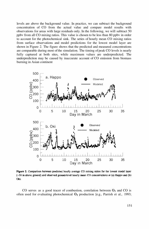
levels are above the background value. In practice, we can subtract the backgroundconcentration of CO from the actual value and compare model results withobservations for areas with large residuals only. In the following, we will subtract 50ppbv from all CO mixing ratios. This value is chosen to be less than 80 ppbv in orderto account for the photochemical sink. The series of hourly mean CO mixing ratiosfrom surface observations and model predictions for the lowest model layer areshown in Figure 2. The figure shows that the predicted and measured concentrationsare comparable during most of the simulation. The timing of peak CO levels is nearlyfully captured at both sites, while maximum values are underpredicted. Theunderprediction may be caused by inaccurate account of CO emission from biomassburning in Asian continent
CO serves as a good tracer of combustion, correlation between and CO isoften used for evaluating photochemical production [e.g., Parrish et al., 1993;
151

Mauzerall et al., 2000]. Checking the observed time series of in Figure 1 and COin Figure 2, we can find that at Oki Island high concentrations were accompaniedby high CO concentrations. The positive correlation between and CO indicatesthat these high was a photochemical production from anthropogenic emissions.
In the simulation period, there are some ozonesonde data available at Tateno andSapporo in Japan. Figure 3 shows mean vertical ozone profiles from ozonesonde andmodel prediction at Tateno (9 sondings at about 15:00 JST on March 2, 6 9, 13, 16,19, 23, 26, and 30) and Sapporo (4 sondings at about 15:00 JST on March 2, 18, 25,and 30). The Tateno site is located at latitude, longitude, and altitude of 36°3’N,140°6’E, and 31 m above sea level, and the Sapporo site – 43°3’N, 141°20’E, and 19m. From the figure we can see that the predicted concentrations are in goodagreement with ozonesonde data at upper layers, which shows the PV is a goodindicator of stratospheric ozone.
Comparison of model simulations with near surface observations of O3 and CO,and ozonesonde data indicates that the horizontal and vertical distributions oftropospheric ozone are reasonably well captured in the simulation. Now we try toquantify the contributions from transport versus chemical processes. Figure 4 showssources and sinks of ozone in an area of around Okinawa (remote area)in Japan and Shanghai (source area) in China in March of 1998. In the figure positivevalues indicate ozone gain, and negative values indicate ozone loss.
From Figure 4 we find that in the surface layer (~100m), the transport processesmay play more important roles than photochemical factors in determining ozoneconcentrations. In Shanghai area photochemical production is low in the surfacelayer because of titration of excess emission of NO and CO, dry deposition iscompensated mainly by horizontal transport and downward transport from abovesurface layer, where is favorable for ozone production.
In the boundary layer (~1000m), ozone is vertically transported out due to activeconvection in the springtime, and the supply and loss of boundary layer ozone is
152
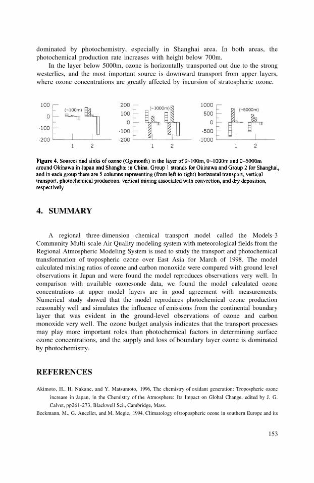
dominated by photochemistry, especially in Shanghai area. In both areas, thephotochemical production rate increases with height below 700m.
In the layer below 5000m, ozone is horizontally transported out due to the strongwesterlies, and the most important source is downward transport from upper layers,where ozone concentrations are greatly affected by incursion of stratospheric ozone.
4. SUMMARY
A regional three-dimension chemical transport model called the Models-3Community Multi-scale Air Quality modeling system with meteorological fields from theRegional Atmospheric Modeling System is used to study the transport and photochemicaltransformation of tropospheric ozone over East Asia for March of 1998. The modelcalculated mixing ratios of ozone and carbon monoxide were compared with ground levelobservations in Japan and were found the model reproduces observations very well. Incomparison with available ozonesonde data, we found the model calculated ozoneconcentrations at upper model layers are in good agreement with measurements.Numerical study showed that the model reproduces photochemical ozone productionreasonably well and simulates the influence of emissions from the continental boundarylayer that was evident in the ground-level observations of ozone and carbonmonoxide very well. The ozone budget analysis indicates that the transport processesmay play more important roles than photochemical factors in determining surfaceozone concentrations, and the supply and loss of boundary layer ozone is dominatedby photochemistry.
REFERENCES
Akimoto, H., H. Nakane, and Y. Matsumoto, 1996, The chemistry of oxidant generation: Tropospheric ozone
increase in Japan, in the Chemistry of the Atmosphere: Its Impact on Global Change, edited by J. G.
Calvet, pp261-273, Blackwell Sci., Cambridge, Mass.
Beekmann, M., G. Ancellet, and M. Megie, 1994, Climatology of tropospheric ozone in southern Europe and its
153

relation to potential vorticity, J. Geophys. Res., 99:12,841-12,853.
Benkovitz, C. M., M. T. Schultz, J. Pacyna, L. Tarrason, J. Dignon, E. C. Voldner, P. A. Spiro, J. A. Logan, and
T. E. Graedel, 1996, Global gridded inventories of anthropogenic emissions of sulfur and nitrogen, J.
Geophys. Res., 101:29,239-29,253.
Byun, D. W., and J. K. S. Ching, ed., 1999, Science algorithms of the EPA Models-3 community multi-scale air
quality (CMAQ) modeling system, NERL, Research Triangle Park, NC.
Carmichael, G. R., I. Uno, M. J. Phadnis, Y. Zhang, and Y. Sunwoo, 1998, Tropospheric ozone production and
transport in the springtime in east Asia, J. Geophys. Res., 103:10,649-10,671.
Ebel, A., H. Hass, H. Jakobs, M. Laube, M. Memmesheimer, and A. Oberreuter, 1991, Simulation of ozone
intrusion caused by tropopause fold and cut-off low, Atmos. Environ., 25A:2131-2144.
Lee, S.-H., H. Akimoto, H. Nakane, S. Kurnosenko, and Y. Kinjo, 1998, Increase of tropospheric ozone at
Okinawa, Japan, Geophys. Res. Lett., 25:1637-1640.
Liu, S. C., M. Trainer, F. C. Fehsenfeld, D. D. Parrish, E. J. Williams, D. W. Fahey, G. Hubler, and P. C. Murphy,
1997, Ozone production in the rural troposphere and the implications for regional and global ozone
distributions, J. Geophys. Res., 92:4191-4207.
Liu, S.C., et al., 1996, Model study of tropospheric trace species distributions during PEM-West A, J. Geophys.
Res., 101:2073-2085.
Mauzerall, D. L., D. Narita, H. Akimoto, L. Horowitz, S. Walters, D. A. Hauglustaine, and G. Brasseur, 2000,
Seasonal characteristics of tropospheric ozone production and mixing ratios over East Asia: A global
three-dimensional chemical transport model analysis, J. Geophys. Res., 105:17,895-17,910.
Oliver, J. G. J., A. F. Bouwman, C. W. M. Van der Mass, J. J. M. Berdowski, C. Veldt, J. P. J. Bloos, A. J. H.
Visschedijk, P. Y. J. Zandveld, and J. L. Haverlag, 1996, Description of EDGAR Version 2.0: A set of
global emission inventories of greenhouse gases and ozone-depleting substances for all anthropogenic
and most natural sources on a per country basis and on grid, National Institute of Public Health and
the Environment (RIVM) report no. 771060 002 / TNO-MEP report no. R96/119.
Oltmans, S. J., and H. Levy II, 1992, Seasonal cycle of surface ozone over the western North Atlantic, Nature,
358:392-394.
Oltmans, S. J., and H. Levy II, 1994, Surface ozone measurements from a global network, Atmos. Environ.,
28:9-24.
Oltmans, S. J., et al., 1998, Trends of ozone in the troposphere, Geophys. Res. Lett., 25:139-142.
Parrish, D. D., J. S. Holloway, M. Trainer, P. C. Murphy, G. L. Forbes, and F. C. Fehsenfeld, 1993, Export of
North American ozone pollution to the North Atlantic Ocean, Science, 259:1436-1439.
Penkett, S., N. Blake, P. Lightman, A. Marsh, P. Anwyl, and G. Butcher, 1993, The seasonal variation of
nonmethane hydrocarbons in the free troposphere over the North Atlantic Ocean: Possible envidence for
extensive reaction of hydrocarbons with the nitrate radical, J. Geophys. Res., 98:2865-2885.
Pielke, R. A., W. R. Cotton, R. L. Walko, C. J. Tremback, W. A. Lyons, L. D. Grasso, M. E. Nicholls, M. D.
Moran, D. A. Wesley, T. J. Lee and J. H. Copeland, 1992, A comprehensive meteorological modeling
system – RAMS, Meteorol. Atmos. Phys., 49:69-91.
Pochanart, P., J. Hirokawa, Y. Kaji, H. Akimoto, and M. Nakao, 1999, Influence of regional-scale anthropogenic
activity in northeast Asia on seasonal variations of surface ozone and its precursors observed at Oki,
Japan, J. Geophys. Res., 104:3621-3631.
154

DISCUSSION
P. BUILTJES
M. ZHANG
Do I understand correctly that the Spring time observed ozonemaximum is due to production, not to stratospheric intrusions ?
Yes. The model simulation shows that subsidences of rich airfrom stratosphere can cause high surface concentrationoccasionally, but on monthly average the Spring ozone maximum iscaused by photochemical production based on budget analysis.
155

This page intentionally left blank
The term “smog” has been used loosely to refer to air urban pollution in general withthe consensus that these pollutants are formed through a transformation process, veryoften involving photochemistry. For most urban areas, smog encompasses at least threedistinct, yet inter-related, pollutants: ozone, and suspended particulates. Air qualityobjectives (AQO) or standards are usually set for each of these pollutants. Despite theseparate consideration of these pollutants, attention has traditionally been focused onozone as an indication of photochemical activities and hence the severity of otherphotochemical smog species. However, it has been known that ozone andconcentrations at specific times and locations usually bear an inverse relationship to eachother – high ozone is usually accompanied by low and vice versa – and thatchemical and photochemical activities enhance the production of secondary particulatesfrom gaseous precursors in general. Given that the standards for each of the three smogcomponents are individually health-based and that cumulative or synergistic effects ofthese pollutants are possible, all the components should be considered together in somefashion. The paper discusses how consolidated smog indices are developed tocharacterise the three common components of smog as one phenomenon.
Given the location-specific air pollution signature of each urban area and the infancyof our attempt to quantify total smog, local air quality data must be used to understandthe behaviour of the developed indices. Two sources of data are potential candidates:measurements from air quality monitoring stations or output from simulation models. Theformer usually suffers from spatial patchiness and also potentially from a lack ofunbroken and consistent historical record to allow us to form a comprehensive picture.On the other hand, a comprehensive air quality model, once validated for a location orregion, can be used as a surrogate for measurements and can overcome the problem ofspatial and temporal patchiness. In this paper, we will use a comprehensive model code-named PATH1 for Pollutants in the Atmosphere and their Transport over Hongkongdeveloped from community-based components specifically for the Hong Kong Special
1 Hong Kong Environmental Protection Department, 33/F Revenue Tower, 5 Gloucester Road, Hong KongSpecial Administrative Region, China; e-mail of corresponding author: [email protected]; Tel: 852-2594-6303;Fax: 852-2827-8040.
TESTING SMOG INDICES USINGA COMPREHENSIVE MODEL
Christopher Fung, Hin-Chung Lau, Linda Yu, Kenneth Leung, Alick Chang1
1. INTRODUCTION
Air Pollution Modeling and Its Application XV, Edited byBorrego and Schayes, Kluwer Academic/Plenum Publishers, New York, 2002 157

Administrative Region (HK) of China to provide data to analyse the behaviour of theproposed smog indices. This 3-D modeling system puts together MM5, EMS-95 andSAQM in a consistent framework to simulate meteorology, emission and air quality,respectively and is set up on a polar stereographic grid with five nested domains ofdecreasing grid spacing (by factor of three) centering over HK. The largest domain hashorizontal grid spacing of 40.5 km and extends west to the Himalayas, north to centralChina, east to the central Pacific and south to the Philippines while the 1.5km spacingdomain covers all of HK. Simulations on this l.5km-spacing domain are used for thispaper. A two-day smog episode (19-20 August 1996) with generally high concentrationsof all smog components is simulated for testing the indices. Though we are using HK’sAQO (Table 1) to develop our very preliminary smog indices and will be studying thebehaviour of such indices over HK, the work is intended to demonstrate the idea forurban areas in general.
Three approaches based on different assumptions can be used to characterise smog:1. An index based on one species concentration normalized by the species’ AQO.2. The maximum of the normalized indices of the smog components as defined above.3. A single index consolidated by adding the normalized indices as defined in 1 above ofeach of the three components.
Calculating the indices based on the last two approaches is complicated by the factthat for some smog species, different AQOs are defined based on averaging times. Table1 shows that HK has a 1-hr objective for and a 1-hr as well as a daily objective for
For respirable suspended particulates (RSP), no 1-hr objective has beenpromulgated, but daily and annual objectives exist. On the other hand, model data aregenerated hourly and this preliminary study is only limited to using one model-simulatedepisode spanning two days.
Another set of complications arises from the fact that RSP is defined as all suspendedparticulates with diameter below while the health and visibility effects which are ofmost concern to the public are most pronounced for fine suspended particulates (FSP)defined as particles having diameter below It is this fraction of RSP that are theactive component of “smog.” For HK, RSP has an AQO while FSP does not. It has alsobeen thought that a significant portion of these fine particulates are formed from gas toparticulate transformation followed by coagulation and referred to as secondaryparticulates. On the other hand, the model used in this attempt, though differentiatingbetween FSP and RSP emissions as well as calculating gas to particulate transformation,does not follow the growth of these secondary particulates in size. Given these difficulties,we have opted for the following compromises and assumptions in defining the latter twotypes of smog index which are all based on the maximum concentrations for the
158
2. DEVELOPMENT OF TESTING SMOG INDICES

appropriate averaging times produced by the model during the simulation period:1. Two individual indices (I) for are formed from the 1-hr and daily AQOs throughnormalizing (i.e. dividing by the AQO values of corresponding averaging time.)2. The annual AQO for RSP is ignored because it is too long for smog episodes in HKand an hourly AQO for RSP is invented for this study from the daily AQO by applyingthe same ratio (0.5 for hourly to daily) that is in the Japanese Air Quality Standards2.3. To come up with an FSP testing “standard” from RSP, the ratios between the U.S.proposed FSP and RSP standards3 for one-day and one-year averaging times are averagedand applied to HK’s AQO.4. The modelled concentration for FSP is defined as the sum of primary FSP and allsecondary particulates since most secondary particulates are believed to be smaller than
in diameter.5. The hourly and daily FSP component indices are calculatedbased on 3. and 4. above in the same way as was done for in 1 above.6. Based on the above five individual indices (I), and the three approaches enumeratedpreviously, the following five consolidated indices (CI) are defined:
The modeled data can support the choice of three types of conveniently definedspatial coverage for analysis to form a single view of smog over an area (see Figure 1):1. At some model grid cells in which air quality monitoring stations are located totaling15 for our study area;2. At some heavily populated regions scattered over the study area defined just for thepurpose of this preliminary study which number 8 and occupy 55 grid cells with eachregion composed of between 4 and 11 grid cells;3. Over the entire land area of HK including the major outlying islands which isrepresented by a total of 621 grid cells out of a total of 49 x 49 grid cells in the domaincurrently considered.
Figure 2 shows a plot of the five individual indices (with average and standarddeviations as appropriate) calculated for the three coverages. The following features areof note:1. the average of the indices vary from 35 to 53 showing a 40% difference between thehighest and lowest. The average of the indices for the stations cover approximately thesame range (37-53) while that of the regions cover a smaller range between 35 and 48.2. the order of the station and region data for any index can be quite different indicating
159
3. Testing the Developed Smog Indices for the Base-Case
a.b.c.d.e.
It is noted that the indices defined as daily still retains the hourly ozone componentand no attempt is made to make it consistent because defining a 24-hr ozone standard orobjective is not very meaningful given our understanding of short-term behaviour ofozone. The maximum modeled concentration over the averaging period is used for indexvalue calculation.
= maximum hourly normalized ozone concentration

that the relative severity of smog is not represented by the stations if the region data,being more representative, are taken to be the standard.3. the corresponding averages of the indices for stations and regions do not differ bymore than 23% while some can be as small as 5% (indices 1 and 2 based on hourly ozoneand indicating that the model-represented stations, take together, can represent allland area to within this accuracy.
160

4. both the averages and standard deviations of the indices of the regions areconsistently smaller than that for the stations, indicating the averaging effect ofconsidering a wider area in constructing an index and the stability that can result.5. the value for the all-land index is higher than its “station” and “region” counterpartsfor by more than 10%, but lower by a larger percentage for the and FSP hourlyand daily indices. Though the station and region values for the first index based on arelower than all their other counterparts based on other species (except for the very last oneof maximum daily FSP over the regions), the all-land value for this ozone-based index isthe highest among all its counterpart. This is a clear indication of the phenomenon thatis usually strongest away from urban areas where its precursors are emitted while high
and FSP are more urban phenomena. This reasonable behaviour of the indices alsogives them credence. More so, the importance of taking an appropriate spatial average ishighlighted.
The consolidated indices based on formulae (1)-(5) above are plotted in Figure 3. Thefirst column of this plot would be the same as that in Figure 2 since the two indicesare identical – based solely on maximum hourly ozone concentration. As far as spatialrepresentativeness of these consolidated indices is concerned, points 2 and 4 above forthe individual indices also apply here to the consolidated indices. The next two indices,
show higher values than due to the “pick-the-winner” approach.What is strikingly different is the magnitude of the last two consolidated indices whichare approximately two and a half to three times that of the previous three indices. Yet thisis to be expected given that all the component indices shown in Figure 2 areapproximately of the same magnitude and it also points out the inadequacy of using anyone individual index to represent smog. The values of the first three indices calculatedover all-land are the same, indicating that ozone has dominated on this spatial scale. Theall-land values for and are lower than their station and regioncounterparts, indicating dominance on this spatial scale by and FSP whoseconcentrations are generally lower away from populated areas and monitoring stations.
161
and
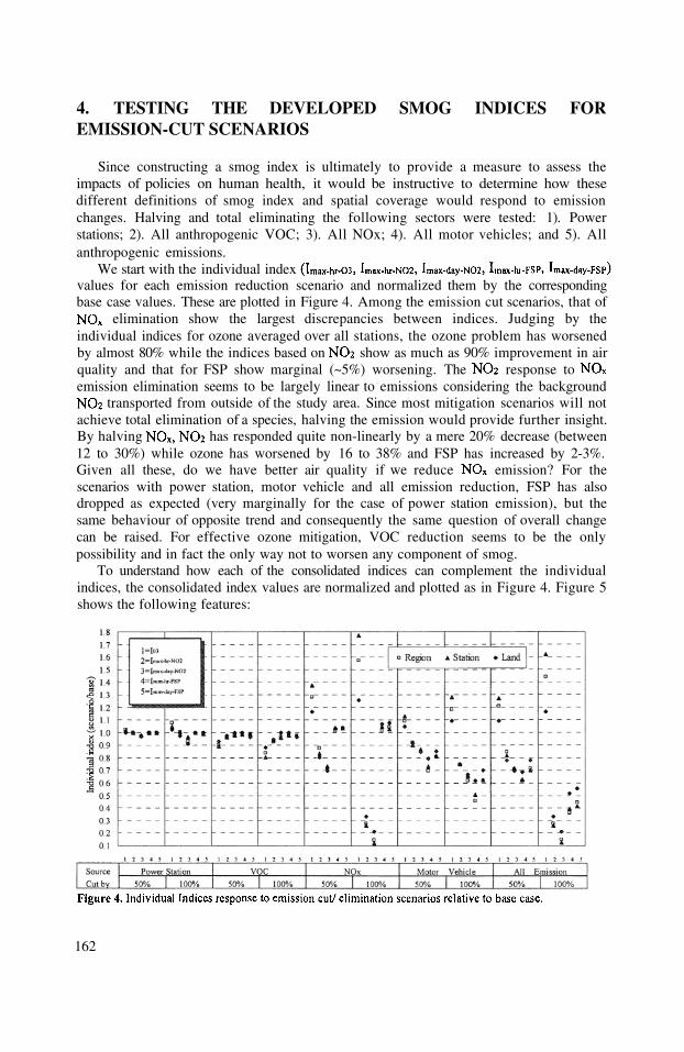
Since constructing a smog index is ultimately to provide a measure to assess theimpacts of policies on human health, it would be instructive to determine how thesedifferent definitions of smog index and spatial coverage would respond to emissionchanges. Halving and total eliminating the following sectors were tested: 1). Powerstations; 2). All anthropogenic VOC; 3). All NOx; 4). All motor vehicles; and 5). Allanthropogenic emissions.
We start with the individual indexvalues for each emission reduction scenario and normalized them by the correspondingbase case values. These are plotted in Figure 4. Among the emission cut scenarios, that of
elimination show the largest discrepancies between indices. Judging by theindividual indices for ozone averaged over all stations, the ozone problem has worsenedby almost 80% while the indices based on show as much as 90% improvement in airquality and that for FSP show marginal (~5%) worsening. The response toemission elimination seems to be largely linear to emissions considering the background
transported from outside of the study area. Since most mitigation scenarios will notachieve total elimination of a species, halving the emission would provide further insight.By halving has responded quite non-linearly by a mere 20% decrease (between12 to 30%) while ozone has worsened by 16 to 38% and FSP has increased by 2-3%.Given all these, do we have better air quality if we reduce emission? For thescenarios with power station, motor vehicle and all emission reduction, FSP has alsodropped as expected (very marginally for the case of power station emission), but thesame behaviour of opposite trend and consequently the same question of overall changecan be raised. For effective ozone mitigation, VOC reduction seems to be the onlypossibility and in fact the only way not to worsen any component of smog.
To understand how each of the consolidated indices can complement the individualindices, the consolidated index values are normalized and plotted as in Figure 4. Figure 5shows the following features:
162
4. TESTING THE DEVELOPED SMOG INDICES FOREMISSION-CUT SCENARIOS

1. From the point of view of where the indices fall with respect to the base case, thescenarios can be classified into three types:
a). unequivocal improvement, i.e. all consolidated index values are below 1.0; withinthis category fall only the two VOC scenarios and the one scenario in which allanthropogenic emission in the study area are eliminated. Nevertheless, most of theindices in this group fall within the 0.9 to 1.0 range or very close to 0.9;b). unequivocal deterioration, i.e. all consolidated index values are at 1.0 or above;only the case of eliminating all power station emissions belong to this type; thoughthis may be explained by the increase in ozone when the from power stations iseliminated, it is somewhat unexpected and merits further exploration;c.) mixed results, i.e. the consolidated index values are scattered about both sides ofthe 1.0 line; within this group are the rest of the scenarios though it may be argued thatthe first case is rather marginal.
2. If it is taken that the order of the arrangement of the consolidated indices represents ageneral progression from less to more comprehensiveness of our measurement methodusing indices (summing is more comprehensive than taking maximum than only lookingat ozone; daily averaging more comprehensive than hourly averaging), then the slope thatbest fits the points within each scenario would carry a physical meaning (though arigorous mathematical calculation of the slopes would not be very meaningful due to thedifficulties in quantifying the comprehensiveness of each of the indices) and the scenarioswould fall into two categories with:
a). positive visual slopes indicating that as the measurement index is made morecomprehensive, the smog situation is revealed to be worse; only the two VOC cutscenarios fit this category though it must be emphasized that both show netimprovements relative to the base case;b). negative visual slopes which indicate the opposite of a.) above; all other scenarioswould fall under this category and the more negative is the slope the greater is thespread of the index values; contrary to a) above, almost all scenarios showimprovement as well as deterioration with respect to the base case depending on whichindex is used as the measure.
3. The large range of the spread of indices for some scenarios with mixed results (1cabove) indicate that the choice of index, like the individual indices, can still give
163

diametrically opposite results for the same emission reduction / elimination scenarios. Forthe scenario with eliminated from the study area, for stations indicate a 74%increase in smog while and indicate up to a 20% decrease in smog, a 90+percent difference. The same is true for the scenario when all anthropogenic emissions inthe study area are eliminated: increases by 45%; decreases by 47%.4. The all-land values for the indices vary over the smallest range among the threespatial coverages and this is also true of the individual indices in Figure 4. This howeverdoes not preclude the observation in 3 above that diametrically opposite conclusions caneven be drawn from index values averaged over such a large land area. Large spatialaveraging of ozone is no substitute for considering all the components of smog.5. The all-land values for are identical for all the scenariosconsidered here indicating that for the day simulated, no amount of emission fiddling canchange the fact that ozone dominates if all land area is considered. That does not meanthat emission changes cannot bring about significant improvement over all the land areaas seen in the large range of index values that exists between scenarios.6. Relative to the individual indices, these consolidated index values span over a muchsmaller range with the smallest value for the case of total emission elimination being 0.57versus the corresponding individual index value of 0.12.
The lessons gleaned from the above discussion show that a numerical model is aconvenient tool to analyse the behaviour of the experimental indices. From these indices,it is clear that smog in an urban area must be viewed in total to avoid wrong conclusionsbased on an incomplete consideration. The best indices should be the ones based on asummation of all smog components though a rigorous scientific proof is not yet possible.
We have only used three components and combined them linearly here as apreliminary exploration. Other components and methods of combination can be tried. Tomore firmly utilize the concept of consolidated smog indices, health based air qualitystandards with consistent averaging time must be set and the synergistic effects of thecomponents of smog must be explored through health study and built into thecombination. Further explorations with other emission scenarios, smog episodes,boundary conditions and in other urban settings can be made to probe the behaviour ofthe indices further.
ERM-HK (2001) Territory-wide Air Quality Modelling System: Final Report,submitted to the Hong Kong Environmental Protection Department, 132pp.Environmental Quality Standards in Japan – air quality; available onhttp://www.eic.or.jp/eanet/en/index.htmlProposed Air Quality standards for the U.S.; available onhttp://www.epa.gov/airlinks/airlinks4.html
164
5. SUMMARY AND DISCUSSIONS
DisclaimersThe views expressed in this paper represent only that of the authors.
References1.
2.
3.

F. LEFEBRE You showed us that you go down in resolution by an order ofthree (40.5-13.5 ... 0.5). Can you comment on this ? On whichbasis did you make your choice ? Did you do sensitivityexperiments ? What is most sensitive MM5, CTM, emissions ?
Ch. FUNG The factor of 3 step down in grid spacing was recommended bythe MM5 developer considering the stability of the numerics andthe rapidity in getting to the area of interest. This ratio was thenapplied to SARM + EMS95. We did not do further sensitivityexperiments.
G. GENIKHOVICH When calculating your indices, you were assuming that thetoxciticy of different species at the level of two air qualitystandards (objectives, for example), is the same. Why do youthink so ?
Ch. FUNG This was based on the common sense assumption and alsobecause we have worked on synergistic effects. We can build infurther refinements if information is available.
A. EBEL What is the accuracy of the (and other) emission andobservational data used for the study ?
Ch. FUNG We have a fairly good estimate of emissions within the HongKong domain, but the further we go away from Hong Kong, thegreater the uncertainty. A recent study over the Pearl River Deltawhich is the region immediately to the north of Hong Kongsuggests a factor of 2 difference in the and VOC estimates.Further out in China/Asia, a preliminary comparison indicates thatour estimates based on GEIA/EDGAR differ from that of theTrace-P (David Street, Argonne National Lab.) database by afactor of 2-6 depending on the species. Our first task in modelimprovement is to narrow down the uncertainties in the emissions.The other observational data, e.g. monitoring, that we use meetinternational standard.
165
DISCUSSION

This page intentionally left blank
Ozone occurs both in the Earth’s upper atmosphere and at ground level.Stratospheric ozone shields us from the sun’s harmful UV rays. But ground - levelozone is a harmful air pollutant. Surface ozone is formed when NOx emitted by cars,power plants and other industrial sources react chemically in the presence of intensesunlight. High smog levels have been linked to increases in the severity of asthmaattacks and other respiratory health problems. When concentrations rise, even fromrelatively low levels the need for increased medication of asthmatic for especiallychildren and elderly. Otherwise ozone can initiate damage to the lungs as well asdamage to trees, crops and materials.
In urban areas of Turkey, there has been a decrease in concentrations of andparticulates in the 1990s. This is largely due to major changes in the fuel mix used incity centers: domestic coal with high sulfur content has been prohibited for heatingand replaced by imported coal. However, as a result of economic growth and despiteenvironmental protection efforts and significant shifts in energy supply emissions ofNOx are growing at a very high rate. The transportation by car is growing rapidly inthe cities.
According to OECD Report (1999) NOx emissions totaled 844,000 tons in 1997figures, almost two and half times those recorded in 1980s in Turkey. NOx emissionsincreases have accelerated since the early 1990s. Mobile sources contribute 43 percent to total emissions, industrial energy use 19 per cent and power generation 10 percent. Emissions per capita (13.3 kg) are three times less than the OECD average (39.7kg). Total NOx emissions have continued to increase. However we do not haveemission inventory at national and city level for a range of pollutants, including NOxand VOCs.
Istanbul has experienced a rapid growth in urbanization, industrialization and thenumber of motor vehicles. The city experienced serious and TSP air pollutionepisodes in between 1980-1995 with economical expanding. Following the banning ofpoor quality coal burning for domestic and industrial activities in the city, air pollution
* Umit Anteplioglu, Division of Meteorology, Kandilli Observatory, Bosphorus University, KandiliUskudar,Istanbul Turkey, Sema Topcu and Selahattin Incecik, Istanbul Technical University, Department ofMeteorology, Maslak Istanbul Turkey 80626.
Air Pollution Modeling and Its Application XV, Edited byBorrego and Schayes, Kluwer Academic/Plenum Publishers, New York, 2002
AN APPLICATION OF A PHOTOCHEMICALMODEL FOR URBAN AIRSHED IN ISTANBUL
Sema Topcu, and Selahattin Incecik*
1. INTRODUCTION
167

levels were reduced to below the national air quality standards. Fuel switching to thenatural gas and low sulfur coal usage has been taken a role on this variation in the city.In addition, the number of motor vehicles increased at a very fast rate in the city. As aconsequence air quality problems in Istanbul has shifted from conventional airpollution to secondary air pollution in last five years. The history of photochemical airpollution in Istanbul is not long.
In contrast to the increased international concern over ozone, only a very limitedanalysis of the characteristics of urban ground-level ozone has been conducted inTurkey (Topcu and Incecik, 1999; 2001). In spite of the critical ozone levels have notbeen yet measured in the city, ozone potential problem is growing with the rapidgrowing motor vehicles in the city. Although, there has not been yet occurred criticallevels, ozone potential problem is growing with the rapid development oftransportation in Istanbul.
The goal of this study is to apply and assess the temporal and spatial distribution ofphotochemical air pollution in Istanbul. The results based on the discussion of July1999 simulations have been explained by UAM.
Istanbul is located at about 41N and 29E. The city is divided by the Bosphorus asthe European and Asian parts. The population of Istanbul currently stands at about 9.2million and is concentrated along the west and east part of the city.
The climate of Istanbul is governed by the Black Sea and Mediterranean climates.Winter (November to March) is cold and wet. Summer (June to September) is hot andhumid. Insolation in the city is strong; average daily values are of order of insummer. In addition, annual average wind speeds in the city are only 3.0 m/s, 8 %calm hours. Prevailing synoptic winds arriving Istanbul are from the north andnortheast and southeast in winter, northeast and southeast during the summer months.Daily mean temperature in winter is 6.3°C, and 22.4°C in summer. Average dailyvalues of order of in summer and in winter (Topcu et al,1995).
Istanbul has gradually experiencing the highest vehicle densities since 1995.According to the July 1999 figures, a total activity of the vehicles in Istanbul isestimated as an average of 51.3 mil l ion km per day for weekdays 2000).Vehicle emissions account for a significant fraction of the CO emission. There areabout 1.5 million motor vehicles in the city. It is estimated that around 1/3 of thevehicles are in the traffic in a day. There is about 10,000 taxis in the city, driven onthe average 100,000 km/year. Besides LPG has been traditionally used since thebeginning of 1998 in the taxis. Most of the taxis and some of the cars are running onLPG. Furthermore natural gas usage has been started gradually for domestic purposesin late 1993 in the city from Anatolian side of the city.
Ozone is measured using an analyzer of Environment S.A. based onabsorption of UV radiation. The analyzer is AC31M of Environment S.A. The
168
2.GENERAL CHARACTERISTICS OF THE ENVIRONMENT IN ISTANBUL
2.1 Population and Climate
2.2 Data and Region

To identify which meteorological parameters are strongly associated with thefluctuations of daily maximum ozone concentrations and to perceive the temporalvariation patterns of ozone concentrations. We have used a limited period for bothexplaining and understanding of the ozone formation mechanism and to makesimulations both wind field and ozone variation over Istanbul. The available hourlyozone and its precursors data from the months with the potential of the highestphotochemical activity, July 1999 case has been selected for simulations by UrbanAirshed Model.
The shape of the diurnal pattern in hourly ozone concentrations provides clues as tothe formation, scavenging and transport of ozone at a site. As expected that the ozoneprobably of local origin showed a typical diurnal variation. Besides during daytimeozone concentrations starts increasing gradually after sunrise, attains maximum valueduring mid-afternoon hours and then decreases. Concentrations in daytime weretypically three times as large as it’s at nighttime. At nighttime, surface ozone is partlyremoved by the reaction with nitric oxide and deposition. Due to the complexmechanism of the emissions in urban areas, urban ozone formation has beenconcerned. Because the ozone data measured during the period of highest NOxincluding traffic rush hours are somewhat depressed. Ghim et al., (2001) explained thehigh ozone episodes over Seoul area. Riveros et al.,(1998) made an analysis toestimate the relative contribution of and HCs to ozone formation which is themost important air pollutant in Mexico city.
Since no ozone is produced in the absence of sunlight ozone concentrations beganto decrease after sunset, reaching minimum in evening after sunset. Due to there is nophoto oxidation of precursors, ozone levels are observed to be low during nighttime.As it is expected that the daytime increase in ozone concentration is basically due tophoto oxidation of the precursor gases. On the other hand, strong photochemicalproduction and strong convection in the mid-afternoon period caused ozoneconcentrations to reach peak levels in the late afternoon. The hourly measurements ofozone concentration in the urban area started in the beginning of 1998 in two sites ofthe city center. Ozone concentrations are greatly influenced by local meteorologicaland synoptic scale meteorological conditions. A brief overview is given on themaximum concentrations by Topcu and Incecik,(1999). The ozone and NOx data setobtained for 1998-1999 was also discussed by Topcu and Incecik (2001). Maximumozone concentration at the surface is one of the most desired air pollution indicators.The ozone and NOx concentrations exhibited seasonal variations. NOx concentrations
169
3. OVERVIEW OF THE DIURNAL VARIATIONS
measurement system is based on the chemiluminescense effect produced by theoxidation of NO by molecules. is measured by converting it into NO using the
thermal conversion method (GIM, 2000). Furthermore, the hourly data of solarradiation, temperature, wind speed and direction and atmospheric pressure data takenfrom Goztepe meteorological station.
In Istanbul, the Environmental Protection Section of Greater Istanbul Municipalityhas monitored ambient ozone levels since February 1998. There are two monitoringstations are located in densely populated urban areas for Asian and European sidesrespectively. In the year of 2000, the measurements have not been completed forsome technical problems. Incecik and Topcu, (1999; 2001) presented the preliminaryresults on the seasonal variations of ozone and NOx.

reached their highest levels in the winter months with typical values from 76 to 194ug/m3 in both 1998 and 1999 years. The station located in Istanbul Anatolian siteexperiences concentration > from April to July. Additionally, from thedatabase, exceedences have been determined for thresholds of 70ug/m3. It is found 14exceedences of 70ug/m3 in total 16 months. Its about 71% of the total exceedences in1999. According to exceedences (n=40) in total period, the ratio is about58% in 1999 (Topcu and Incecik, 2001)
As a summary, surface ozone in urban area is generated by reactions of NOx andVOCs in the present of sunlight. It is generated from photolysis of nitrogen oxides inthe presence of NMHC and other organics, and is mainly associated with caremissions in urban areas. This production mechanism can be easily understood withthe diurnal variation of ozone in urban atmosphere of Istanbul.
To make a policy decisions concerning emission controls for urban areas,photochemical models have been used. In this study, we used model simulations ofUAM-V which is a three-dimensional photochemical grid model (Anteplioglu, 2001).UAM-V model had never been used before in this area. It was the first time the modelwas used in this city in connection with ozone studies. This model simulates thephysical and chemical processes that affect the concentration of atmosphericpollutants. The UAM-V solves conservation equation for each of approximately 30chemical species. This equation includes terms representing; advective transport,horizontal and vertical diffusion, emissions, chemical reactions and deposition (SAI,1996). UAM-V generates three-dimensional gridded fields of each simulated chemicalspecies as hourly output.
In order to better understand the impact of the winds on the surface ozoneconcentrations, it is necessary to determine the region’s airflow, such as sea-breezecirculations. In this study, simulations with the Urban Airshed Model were performed.An application of UAM-V including meteorology, chemistry and emissions based onreal ambient conditions is used. However, simulations with the UAM were performedusing limited data set in Istanbul. Data from surface meteorological stations andupper air station were obtained from Turkish State Meteorological Service. Tocompare the wind fields, UAM runs were made. Figures 1 and 2 explain the modelsimulations on July 11, 1999 for 13:00 and 17:00 LST (Anteplioglu, 2000). Thedominant winds in July which is a typical summer month, are northeasterly. The weaklocal sea-breeze circulations can clearly be seen following the heating hours overIstanbul (Fig. 1). These kind of circulations are disappearing at the late afternoonhours (Fig. 2). The region experiences differential heating and cooling due to thetopographical conditions.
170
4. URBAN AIRSHED MODEL
4.1. Mobile Emissions
To obtain the realistic emissions in the city it is necessary to know the actual trafficpatterns for weekdays and weekend in July 1999. On-road mobile emissions wereestimated by using emission factors. Traffic volume, speed and temporal distributionwere used for emission inventory modeling. Table 1 gives the estimated total mobileemissions for July 10, 1999. These inventories were used to produce UAMsimulations to study the effects of the factors on emissions and the effects of thedifferent emissions on precursor and ozone concentrations.

Temporal and Spatial variation of surface ozone concentrations predicted byUAM-V are shown in Figs.3 and 4. Higher concentrations of ozone are observed nearthe southwest coasts of Istanbul. Surface ozone concentrations for 13:00 LST and17:00 on July 1999 indicate the ozone cumulating at the southwest of the city.However, higher concentrations are usually observed during intense solar radiationtimes and moved to inland areas following the sea breeze penetration. This resultsupports the effect of local sea-breeze circulation over the area.
Table 2 compares the results of RMSE and the ratios of sigma values of predicted andobserved concentrations.
171
5. THE RESULTS AND DISCUSSION
In this study simulated daily patterns by considering weekdays and weekends forJuly 1999 showed reasonable distribution. The findings support the Wakamatsu et al.(1996;1999)’s results. Wakamatsu (1999) investigated a relationship betweenemission intensity of NOx, NMHC and O3 concentration covering Tokyo andsurrounding areas by using UAM.
As a summary, ozone is formed through non-linear interactions between chemicalreactions and atmospheric variables. The resulting increased photochemical precursorshave forced environmental policy makers to recognize the potential urban ozoneproblem. For this purpose we presented the urban ozone levels and hourly simulationsby using a three-dimensional Eulerian photochemical simulation model results in thecity.
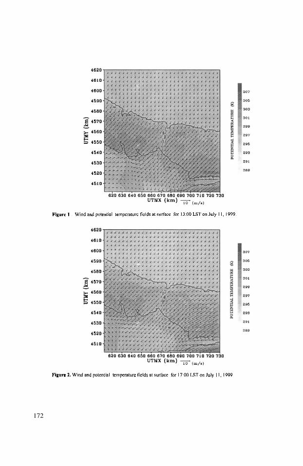
172

173

Anteplioglu, U., 2000, Istanbul Bolgesinde yüzey ozonun fotokimyasal-dinamik bir modelle incelenmesi (inTurkish), PhD. Thesis, Istanbul Technical University, 147.
Ghim.Y.S., Oh, H.S., Chang, Y.S., 2001, Meteorologically effects on the evalution of high ozone episodesin the Greater Seoul area, J.Air &Waste Manage. Assoc. 51,185-202.
GIM , 2000, Greater Istanbul Municipality data archive.OECD Report, 1999 Turkey,Environmental Peformance Reviews, 186.Riveros H.G., Arriaga, J.L., Tejede, J., Julian-Sanchez.A., Riveros-Rosas, H., 1998, Ozone and its
precursors in the atmosphere of Mexico City. J.Air &Waste Manage. Assoc. 48,866-871SAI, 1996Topcu, S,Dilmac, S, Aslan Z., 1995, Study of hourly solar radiation data in Istanbul, Renewable Energy,
6,171-174.Topcu, S., Incecik, S., 1999, Istanbul’da sehir ozone seviyelerine ait ilk olcumlerin degerlendirilmesi (in
Turkish), National Symposium on Air Pollution and Control, Izmir,279-285.Topcu, S., Incecik, S., 2001, Surface ozone measurement and meteorological influences in the urban
atmosphere of Istanbul, Int J.of Environment and Pollution (submitted)Wakamatsu. S., Ohara, T., Uno, I., 1996, Recent trends in precursor concentrations and oxidant distribution
in the Tokyo and Osaka areas. Atmospheric Environment, 30, 715-721Wakamatsu S., Itsushi, U., Toshimasa, O., Kenneth, L.S.,1999, A study of the relationship between
photochemical ozone and its precursor emissions of nitrogen oxides and hydrocarbons in Tokyo andsurrounding areas. Atmospheric Environment, 33,3097-3108
174
5. REFERENCES

Did you make an estimate of the inflow of ozone into the Istanbularea versus the production of ozone by Istanbul emissions ?
We did not apply a model yet for the inflow of ozone. However weestimate the inflow of ozone from the south parts of the city andsouth east part of the surrounding areas (Gebre and Kocacliindustrial area).
175
DISCUSSION
P. BUILTJES
S. INCECIK

This page intentionally left blank
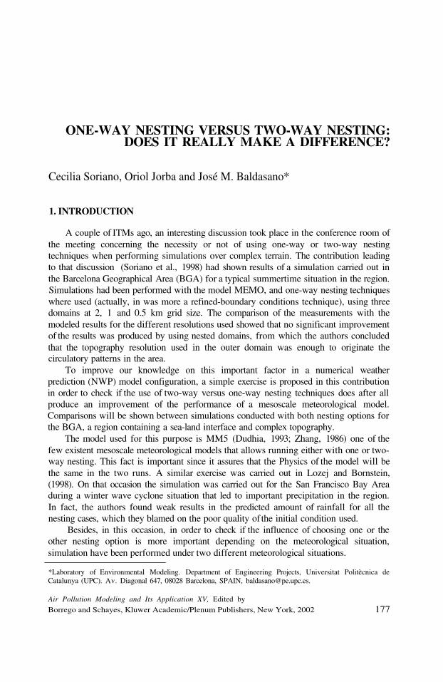
ONE-WAY NESTING VERSUS TWO-WAY NESTING:DOES IT REALLY MAKE A DIFFERENCE?
Cecilia Soriano, Oriol Jorba and José M. Baldasano*
1. INTRODUCTION
A couple of ITMs ago, an interesting discussion took place in the conference room ofthe meeting concerning the necessity or not of using one-way or two-way nestingtechniques when performing simulations over complex terrain. The contribution leadingto that discussion (Soriano et al., 1998) had shown results of a simulation carried out inthe Barcelona Geographical Area (BGA) for a typical summertime situation in the region.Simulations had been performed with the model MEMO, and one-way nesting techniqueswhere used (actually, in was more a refined-boundary conditions technique), using threedomains at 2, 1 and 0.5 km grid size. The comparison of the measurements with themodeled results for the different resolutions used showed that no significant improvementof the results was produced by using nested domains, from which the authors concludedthat the topography resolution used in the outer domain was enough to originate thecirculatory patterns in the area.
To improve our knowledge on this important factor in a numerical weatherprediction (NWP) model configuration, a simple exercise is proposed in this contributionin order to check if the use of two-way versus one-way nesting techniques does after allproduce an improvement of the performance of a mesoscale meteorological model.Comparisons will be shown between simulations conducted with both nesting options forthe BGA, a region containing a sea-land interface and complex topography.
The model used for this purpose is MM5 (Dudhia, 1993; Zhang, 1986) one of thefew existent mesoscale meteorological models that allows running either with one or two-way nesting. This fact is important since it assures that the Physics of the model will bethe same in the two runs. A similar exercise was carried out in Lozej and Bornstein,(1998). On that occasion the simulation was carried out for the San Francisco Bay Areaduring a winter wave cyclone situation that led to important precipitation in the region.In fact, the authors found weak results in the predicted amount of rainfall for all thenesting cases, which they blamed on the poor quality of the initial condition used.
Besides, in this occasion, in order to check if the influence of choosing one or theother nesting option is more important depending on the meteorological situation,simulation have been performed under two different meteorological situations.
*Laboratory of Environmental Modeling. Department of Engineering Projects, Universitat Politècnica deCatalunya (UPC). Av. Diagonal 647, 08028 Barcelona, SPAIN, [email protected].
Air Pollution Modeling and Its Application XV, Edited by
Borrego and Schayes, Kluwer Academic/Plenum Publishers, New York, 2002 177

2. NESTING TECHNIQUES FOR MESOSCALE MODELING
It is well known the importance of the orographic features in a given region in theestablishment of the circulatory patterns of air masses in general and air pollution inparticular within its airshed. For a mesoscale model to be capable of reproducing thisbehavior, it is necessary to introduce a well resolved terrain file, with a resolution suchthat these orographic features are not smoothed away. The other fact is that thesimulation domain has to be large enough to include all the terrain characteristics that arebelieved to participate in the circulation of air masses, and these can often be far awayfrom the study area. Both conditions would lead to the ideal situation of simulating over alarge domain with a very high resolution. However, computational and practicalconstrains do not allow this approach to be used, since it would require simulation over alarge number of cells at small time steps (due to small cell size), and therefore largesimulation times and memory requirements.
Nesting techniques are the solution to minimize these problems, increasing spatialresolution only in the domains where small scale phenomena might occur and arerelevant for the reproduction of all the forcing mechanisms in the studied area. At thesame time, outer domain (or domains) are also included at a coarser resolution, to assurethe introduction of larger scale forcings into the inner domain. The interaction betweenthe domains is the big issue at this point, and can be carried out basically through todifferent techniques: one-way or two-way nesting.
MM5V3 allows the choice of any of these two different types of interaction betweenthe coarser and the inner domains. In the one-way nesting, the model is first run for theouter domain to create an output that is interpolated in time and space to supply the nestas a boundary file, which is run after the coarser domain has finished. For a two-waynesting, both domains are run at the same time and completely interacting. Nest’s inputfrom the coarse domain is introduced through its boundary, while feedback to the coarsemesh occurs all over the nest interior, as its values are replaced by combination of finedomain values.
In general, two-way nesting is believed to work better because it allows smaller scalefeatures feedback upscale and influence features in the larger scale. However, detractorsof two-way nesting claim that this method somehow “pollutes” results obtained in theouter domain, since they are not longer the solutions of the equations of the system.
3. MODELING SCENARIOS
Two different scenarios have been studied in the BGA in order to see if the chosennesting option in the model was a more determinant factor under some meteorologicalsituation than under others.
In one of the studied cases, the synoptic situation was predominant, and a synopticforcing was introduced through important geostrophic winds in the region. In the othercase, a meteorological situation with weak synoptic forcing was chosen, so thatmesoscale phenomena, induced by the particular topography of the region, would bedominant.
178

3.1. Modeling Domains
Both runs have been performed over the same simulation domains. Four nesteddomains were selected, which essentially covered Europe (Domain 1, D1), the IberianPeninsula (Domain 2, D2), Catalonia (Domain 3, D3) and the BGA (Domain 4, D4). D1has 90x55 54-km cells. D2 has 115x94 18-km cells. D3 has 76x79 6-km cells. D4 has61x61 2-km cells. The vertical resolution consisted for all domains of 23 withthe lowest one situated at 18-m AGL. The upper boundary was fixed at 100 hPa. Timesteps used for the simulations are, respectively, 150, 50,15 and 6 seconds. Initializationand boundary conditions (BC) for the regional model are introduced from reanalysis datafrom the ECMWF global model. Data were available at a 1-degree resolution (100-kmapprox. at the working latitude) at the standard pressure levels every 6 hours.
Figure 1 shows the domains and the topography of D3 and D4. The topography inD3 is essentially dominated by the Pyrenees (a mountain range separating Spain andFrance with mountains of 3000-m height). In the south of the domain, the Ebro Valleywill also play an important role in the establishment of the flow patterns. In D4, mainfeatures are mountain ranges oriented parallel to the coastline and two river valleys atboth sides of the city of Barcelona and running approximately perpendicular to the coast.
Finally, simulations only for D4, including initial and boundary information fromECMWF, have also been performed. They have been used as control cases to see howwell the most inner domain was able to reproduce the circulatory patterns and howdifferent it was from the simulation where information from outer domains is introduced.
3.2. Synoptic Situation: The Western Anticyclonic Advection of May 29, 2000 andthe Summertime Barometric Swamp of August 14, 2000
The synoptic situation on May 29, 2000 can be described, using the typical situationsdescribed for the Iberian Peninsula as a western anticyclonic advection. A high-pressurearea was located over the Atlantic, to the west of the Portugal, advecting westerly windsover most of the Peninsula. The map at 500 hPa also indicated winds from the west (seemaps at http://infomet.am.ub.es/arxiu/avn, April 2001). Radiosondes launched in
179

Barcelona that day confirm the interpretation of the maps (At the web site of the CatalanMeteorological Service, http://www.gencat.es/servmet/radio, April 2001).
Maps corresponding to the of August, 2000 were characterized, both at surfacelevel and in height, by very low baric gradient. This fact, and the strong solar heating,produced the development of mesoscale phenomena. These phenomena in the region aremainly sea-breezes, up-slope and down-slope winds and valley channeled winds. Theheating was so intense that a thermal low started to develop in the Peninsula. Again,synoptic maps for the day are available at the Infomet web site mentioned above.
4. THE SYNOPTICALLY-DOMINATED SITUATION OF MAY 29, 2000
4.1. Control Case: 1 Domain Simulation
Figure 2 shows streamlines simulated by the model at 12 UTC on May 29, 2000 inD4. Comparisons with surface stations are also included. No nesting was performed, anddata from the ECMWF was used for initialization and middle times BC.
Results showed that, even when working with a single domain, the topography in D4had enough resolution to generate the local winds that overwhelmed the synopticwesterly winds, which can only be observed in the left border of the domain.
As far as the comparison with measurements of surface station, note the model’sweak performance at station A, where it failed to reproduce the observed high velocitywinds, although westerly winds are modeled during most of the day (introduced troughthe BC). This station (see Figure1) is located very close to the border of the domain. Themodel reproduced quite well wind speed and direction at station B, located by theseaside, showing the influence of the sea breeze. Station C showed poor results speciallybefore midday, where the models simulated too low winds. Velocities in the afternoonwere more similar to measurements and the agreement in wind directions also improved.
180

4.2. Nested Simulations
Figure 3 shows streamlines simulated by the model at 12 UTC on May 29, 2000. Thedifferent panels show the results over D3 and D4 and when performing one-way or two-way nesting. Note that differences when comparing simulations on D3 with simulation onD4 occur mainly over the region where both domains overlap. The sea-breeze front,identifiable in the one-way simulation by a convergence line, is broken in the two-waysimulation. In D4, the sea-breeze front is also very evident and has almost reached theleft border of the domain, penetrating further inland when performing one-way nesting.
Evaluation of the model performance for the two cases was carried out bycomparison with measurements for the three stations shown in Figure 1 and is included inFigure 4. Comparisons were performed by representing values of measured wind speedand direction with the simulated value in the corresponding cell, both for domains D3 andD4. Nested simulations, when compared with the one-domain simulation shown in Figure2, were able to generate higher wind speeds in all stations, more in agreement withmeasurements. However, speeds in station B, located by the sea and with a highermesoscale influence, showed worst results when using nesting techniques. A slightimprovement of the wind direction was also observed, specially in station C duringnighttime, for the one-way simulation. Finally, when comparing results for the samenesting techniques at the different resolutions (D3 and D4), more differences betweenboth resolution were present when using two-way nesting techniques.
181

5. THE MESOCALE-DOMINATED SITUATION OF AUGUST 14, 2000
5.1. Control Case: 1 Domain Simulation
Figure 5 shows evaluation and streamlines at 12 UTC for the mesoscale-dominatedsituation of August 14, 2000 in D4, for the one-domain no-nested simulation.
Streamlines show a well developed inland sea-breeze flow, which, with the up-valleywinds and the up-slope winds produced a general in-shore circulation. Channeling in theriver valleys was evident. Note the westerly winds at the left border of the domain, resultof the assimilation, in the first rows of cells, of the BC from ECMWF data. Comparisonwith measurements gave reasonable results, showing that the single-domain configurationwas able to generate flows, mainly originated in this scenario by mesoscale phenomena.
182

5.2. Nested Simulations
Figure 6 shows streamlines simulated by the model at 12 UTC on August 14, 2000.The different panels show the results over D3 and D4 and when performing one-way ortwo-way nesting. Differences between both simulations were more evident in this case.Note the presence of differences between simulated fields above the sea. If differencesare observed over the sea, they should have been originated by larger scale phenomenafunneled down to the inner domains. Above the sea, increased resolution does not addfurther topographical information and therefore no additional forcings are fed back to thecoarser domain. As in the previous case, most differences above land were observed onthe region where D3 and D4 overlap (overlapping region shown in top-left panel).
Comparison with surface stations are shown in Figure 7. The performance of themodel was better than for the synoptically-dominated case, specially for one-way nesting.The model reproduced the daily cycle of the wind, and the timing of the swift from thenighttime to the daytime regime was well captured. Winds during nighttime were verylow, which made the prediction of the wind direction difficult. In the one-way simulation,little difference is observed when using a better resolved resolution. Results for D3 andD4 are quite similar. For the two-way simulation, comparisons gave worse results. Forstation B, located by the sea, this was probably due to differences observed in thesimulated fields over the sea when using two-way techniques. Simulated results forstation C showed a lot of fluctuation when using two-way nesting, specially on D4.
183
6. CONCLUSIONS
Simulations performed using different nesting techniques have shown that this factorcan led to rather different results when applied over a domain with complex orographicfeatures. This differences were more evident on situations under low synoptic forcing.For the mesoscale-dominated case, differences obtained by choosing one or anothernesting technique were more important than those produced by using a higher resolutiontopography, and two-way nesting gave worst results. For the synoptically-dominatedcase, the two nesting techniques gave more similar results and differences occurredmainly on the overlapping region of the domains. Predicted values at the differentresolutions are not as similar as in the other scenario and in general gave higher speedsthan observed, indicating that the synoptic component was overestimated by the model.
7. ACKNOWLEDGEMENTS
Authors thank the Spanish Meteorological Institute (INM) for providing ECMWF data and the CatalanMeteorological Service (SMC) for the surface station data. Simulations were run on an HP Exemplar V2500from CESCA. This work was developed under projects IMMPACTE and CICYT REN2000-1754-C02-01/CLI.
8. REFERENCES
Dudhia, J., 1993, A non-hydrostatic version of the Penn State-NCAR mesoscale model: Validation tests andsimulation of an Atlantic cyclone and cold front, Mon. Wea.. Re., 121, pp. 1493-1513.
Lozej, C. and Bornstein, R.D., 1999, Comparison of nesting techniques within a meteorological model, in: AirPollution VII, Brebbia, C. A., Jacobsen, M. and Power, H. ,eds., Comp. Mechanics Pub., pp. 1009-1021.
Soriano, C., Baldasano, J.M. and Buttler, W.T. , 1997, On the application of meteorological models and lidartechniques for air quality studies at a regional scale, in: Air Pollution Modeling and its Application XII,Gryning, S-E. and Chaumeliac, N., eds., Plenum Press, pp. 591-600.
Zhang, D.-L., H.-R. Chang, N.L. Seaman, T.T. Warner and J.M. Fritsch, 1986, A two-way interactive nestingprocedure with variable terrain resolution. Mon. Wea. Rev., 114, 1330-1339
184

DISCUSSION
G. SCHAYES
J. BALDASANO
How can you explain that such a large difference occurs on verticalwind speed in the centre of the domain using 1-way or 2-waynesting ?
The centre of domain 3 corresponds with the upper-left corner ofdomain 4. Instabilities are introduced by the interaction of bothdomains. In this case, the feedback to the coarser mesh makes theresults worse. The lateral boundary placement seems to be animportant fact that highly influence the behaviour working with 2-way nesting.
185

This page intentionally left blank

GLOBAL AND LONG-RANGE TRANSPORT
Chairperson :
Rapporteur :
G. Schayes
A. Voudouri

This page intentionally left blank
APPLYING RISK ASSESSMENT TECHNIQUES TO AIRPOLLUTION MODELLING & ABATEMENT STRATEGIES
Helen M ApSimon, Rachel F Warren and Antonio Mediavilla-Sahagun1
1. INTRODUCTION
Atmospheric modelling is widely used to support decision making on environmentalmatters and pollution abatement. The models used in a regulatory context are often relativelysimple, as compared with a range of other more complex models that reflect atmosphericprocesses in more detail. Model inter-comparisons, validation against measurement, andconventional uncertainty analysis such as sensitivity studies and Monte Carlo analysis, areoften used for “quality assurance” of models.
However from the point of view of a decision maker using results obtained from amodel, such analysis can cause confusion, and lead to difficulties in justifying or agreeingactions to protect the environment. He/she recognises that the application of models inevitablyinvolves assumptions, simplification and uncertainties, but in regulatory contexts models areoften used rather precisely- for example to indicate whether or not a prescribed limit or ceilingis exceeded. The reliability of model estimates, and the robustness of conclusions based onmodel calculations, are therefore important issues. This paper is therefore written from thepoint of view of the model user, and suggests a framework for exploring model uncertaintybased on risk assessment techniques, and in particular HAZard and OPerability studies(HAZOP), to investigate how uncertainties in modelling might affect decisions based onmodel results. It will be illustrated by case studies of long-range transport and transboundaryair pollution, and urban air quality.
2. HAZARD IDENTIFICATION AND RISK ASSESSMENT
In building an engineering plant to produce a specific product risk assessment isundertaken to examine the safety of the plant and fitness for purpose. The same procedurescan be applied to environmental modelling and its reliability with respect to answering thequestions posed. We shall therefore examine some techniques commonly applied to thedesign and specification of industrial plant. Here approaches such as HAZOP are used toidentify how hazardous situation might arise, and the potential consequences. A subsequentrisk assessment would involve a study of the probability of occurrence of such hazards forthose cases where the consequences are significant; and hence to an estimate of potentialoverall “detriment” due to the plant, and decisions on how the risks should be managed orreduced. In applying similar principles to environmental modelling, instead of the safetyissues arising from an industrial plant, we are concerned with the risk that the results derivedfrom the modelling could be misleading to decision makers.
HAZOP techniquesSo let us first consider the formal procedures used to pick out potential problems.
HAZOP techniques(1) provide a systematic method for identifying hazards, treating acomposite system component by component. Thus in an industrial plant each pipe, tank, valve
1 Environmental Measurement, Modelling and Assessment Group, Department of EnvironmentalScience and Technology, Imperial College, Prince Consort Road, London SW7 2BP, United Kingdom.
Air Pollution Modeling and Its Application XV, Edited byBorrego and Schayes, Kluwer Academic/Plenum Publishers, New York, 2002 189

etc would be a separate component, for which the first step in HAZOP would be to define theintended function of each one in turn. For example the intended function of a pipe might be todeliver a certain chemical from one tank to another at a specified rate. The next step is toconsider deviations from this intended function prompted by a number of guide words such as“NOT”, “LESS”/”MORE”, “AS WELL AS”, “REVERSE”, and how such deviations mightoccur. For example let us suppose that the pipe in our example delivers “LESS” chemical thanthe specified rate. This could happen because of a failed valve, or a broken pipe, or becausethe supply tank ran out. The final stage is to consider the consequences of such a deviation,for example an explosion. In many cases deviations identified may lead to no harmfulconsequences, and hence do not need to be considered further.
3. APPLICATION TO ENVIRONMENTAL MODELLING AND ASSESSMENT
Transferring the same approach to environmental modelling involves an analogousbreak-down of the modelling process into component parts. The structure of an integratedassessment approach to an air pollution problem is illustrated in figure 1. Thus suppose we areconcerned with decisions in how to attain certain improvements by some future date. Thismay be for example to improve a long-range problem such as acidification, or a shorter rangeproblem such as urban air pollution and attainment of air quality standards. In both cases it isnecessary to compile information on how current emissions are likely to evolve withoutintervention, “ a business as usual scenario”, and to combine this with atmospheric models todetermine predicted exposure patterns. Environmental criteria need to be established asindicators for protection, either as thresholds below which damage is not expected to occur, orcorresponding to acceptable levels of risk. The difference between the predicted exposure andthe environmental standards is a measure of the “exceedance” that we wish to eliminate. Wethen need to consider the range of options available that could lead to reduction of thisexceedance. Usually this tends to concentrate on emissions, though in the context of urban airquality there may be other effective measures such as pedestrian precincts or low emissionzones that separate the emissions and the exposed population. The aim of the assessment is toinvestigate which options should be implemented in an effective strategy to reduceexceedance, usually with an emphasis on cost-effectiveness. For a systematic evaluation it isnecessary to apply HAZOP to each compartment and link in figure 1.
190

4. CASE STUDY 1: TRANSBOUNDARY AIR POLLUTION
As an illustration we can see how this procedure can be applied in integratedassessment studies of transboundary air pollution in Europe to support development ofprotocols under the Convention on Long-Range Transboundary Air Pollution, CLRTAP.Using the Abatement Strategies Assessment Model, (ASAM)2, we have undertaken extensivestudies in parallel with work by the International Institute for Applied Systems Analysis,IIASA, with their RAINS model3, to address uncertainties in assessing effective strategies tocombat acidification, eutrophication and excess tropospheric ozone. Here we shall concentrateon deposition and the first two effects, considering air concentrations in the second case studyon urban air quality.
Both RAINS and ASAM combine information on emissions from each country inEurope, atmospheric transport and deposition on a continental scale, mapping of “criticalloads” as criteria for environmental protection, and data on potential abatement measures andtheir costs. The aim has been to derive cost effective distribution of emission reductions to bemade by the different countries in Europe in order to reduce exceedance of criticalloads/levels, defined as limits on exposure below which harmful effects are not expected tooccur according to current knowledge. The critical loads are lower in areas of Europe withmore sensitive ecosystems., and clearly some countries contribute more to exposure of thoseareas than others. Targeted strategies4 were therefore required that placed more emphasis onreducing the more damaging emissions. In this paper we shall explore work undertaken toshow that the results obtained from the integrated assessment models provided a robust basisfor negotiation of the Gothenburg protocol agreed in December 1999, and prescribingemission ceilings to be met by each European country by 2010 for and VOCs.
Before seeing how the HAZOP/risk oriented approach can be applied it is helpful toexplain how the ASAM model works, and narrow down the emission scenarios that are ofinterest. The model structure is consistent with figure 1. The emissions data are providedbroken down on a sectoral basis for each country according to a geographical grid spanningEurope, and projected to future situations on the basis of official energy projections, projectedagricultural statistics, and technological and other changes in accordance with currentlegislation. Thus these emissions (the “Current Legislation” scenario) represent the expectedemissions in the target year (2010) without further action taken to reduce them. Theatmospheric transport is based on the EMEP Lagrangian model which has been used to derivesource attribution, calculating the contribution to deposition in each grid cell of the Europeanmap area from each country. It is then assumed that changing the emissions by a certainpercentage changes the corresponding contribution of that country to the deposition in eachgrid cell by the same percentage. In other words a linear relationship is assumed.
The criteria for protection of the environment are represented by critical loads,corresponding to annual average levels of deposition which are sustainable in the long termwithout causing adverse effects. These are defined independently for acidification andeutrophication, and vary geographically and between different types of ecosystem. Ifdeposition is less than the critical load then the corresponding ecosystem is deemed to be“protected”; if it is greater then the ecosystem is at risk, and is “unprotected”. “ Exceedance”of critical loads is a measure of the excess deposition above the critical loads. In practice it isfound that even applying the maximum feasible reductions in emissions regardless of cost, itis not possible to reduce deposition below critical loads everywhere. Hence a lot of discussionhas centred on mapping intermediate target loads that close the gap between the currentdeposition and the critical loads as the ultimate aim4. The intermediate aim is then toeliminate exceedance of the target loads.
Information on the abatement measures is summarised in national cost curves foreach pollutant in each country. These order the measures available in order of increasing costper unit emission reduction, and indicate the cumulative cost of achieving increasinglystringent emission reductions in each country.
191
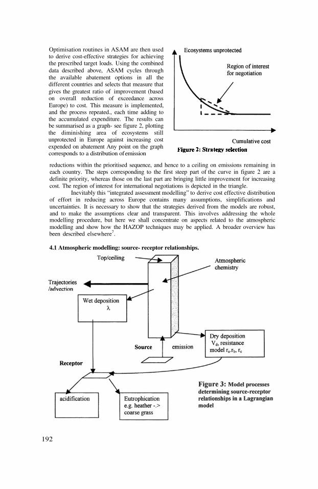
Optimisation routines in ASAM are then usedto derive cost-effective strategies for achievingthe prescribed target loads. Using the combineddata described above, ASAM cycles throughthe available abatement options in all thedifferent countries and selects that measure thatgives the greatest ratio of improvement (basedon overall reduction of exceedance acrossEurope) to cost. This measure is implemented,and the process repeated., each time adding tothe accumulated expenditure. The results canbe summarised as a graph- see figure 2, plottingthe diminishing area of ecosystems stillunprotected in Europe against increasing costexpended on abatement Any point on the graphcorresponds to a distribution of emission
reductions within the prioritised sequence, and hence to a ceiling on emissions remaining ineach country. The steps corresponding to the first steep part of the curve in figure 2 are adefinite priority, whereas those on the last part are bringing little improvement for increasingcost. The region of interest for international negotiations is depicted in the triangle.
Inevitably this “integrated assessment modelling” to derive cost effective distributionof effort in reducing across Europe contains many assumptions, simplifications anduncertainties. It is necessary to show that the strategies derived from the models are robust,and to make the assumptions clear and transparent. This involves addressing the wholemodelling procedure, but here we shall concentrate on aspects related to the atmosphericmodelling and show how the HAZOP techniques may be applied. A broader overview hasbeen described elsewhere7.
4.1 Atmospheric modelling: source- receptor relationships.
192

As indicated above the official model used in the integrated assessment work todescribe the atmospheric transport and derive source- receptor relationships (or “blamematrices”) for sulphur and nitrogen deposition has been the EMEP Lagrangian model8. Thisfollows trajectories backwards from each square in the EMEP grid, every 6 hours. A columnof air is then simulated moving along each trajectory, picking up emissions of and
distinguished by the country of origin, with subsequent chemical transformation and dryand wet deposition processes. In this way the deposition at the terminal point of eachtrajectory can be attributed to sources in the different countries. As compared with a morecomplex Eulerian model, this simpler Lagrangian model can be run over 10 or more years toaverage out substantial inter-annual variations in meteorology.
The first step in applying HAZOP techniques is to define the overall purpose of themodel within the integrated assessment scheme, and then consider the role of the componentparts and links between them. As indicated above the requirement of the atmosphericmodelling is that it should not only calculate maps of total deposition, but should also be ableto indicate what proportion of deposition at any location comes from each country, or fromother sources (e.g. shipping, fluxes from outside Europe). The capability to estimateconcentrations and deposition can be checked against monitoring data. This has already beendone and reported in EMEP annual reports. The more difficult task is that of the sourceattribution. Table 1 gives examples of how HAZOP techniques may be applied to reviewpossible causes for deviation in modelling source-receptor relationships.
In the overall analysis of the integrated assessment modelling, this process has to berepeated in a similar manner to all the other compartments- the projected emissions, thecritical loads and the effectiveness of the abatement measures and their costs. Selectedexperiments can then be performed to test the robustness of the strategies derived for reducingtransboundary air pollution, and the influence of different effects on the emission reduction of
193

individual countries within these strategies. For example the table above suggests studiesa)taking source receptor matrices derived from years with contrasting meteorology toinvestigate the sensitivity to variable trajectory patterns, and b) altering the range of transportby stretching or contracting the “footprint” of deposition from each source, and c) thesensitivity to increasing or decreasing the deposition. Such studies with ASAM have beenreported elsewhere3,5,6,7. Traditional methods using Monte Carlo analysis may also be used-for example to introduce random variations in the costs of abatement measures to reflectvariations between individual sources. However a full Monte Carlo analysis of an atmosphericmodel is extremely time consuming compared with the HAZOP approach described above,and achieves little more than indicating the scale of the variance. Also it does not pick outprocesses that are not included in the model. However complementary modelling studies, forexample to examine the implications of cloud venting and removal (e.g. Kayin9 ), and inter-comparison with more complex models can be very informative
As an example of the selected studies identified above here we can consider theimplications for the overall integrated assessment modelling if the deposition is greater or lessthan the base case estimation, and the implications for the overall integrated assessmentmodelling. This can be combined with uncertainties in the critical loads, since the crucialfactor is the exceedance of the critical loads. This is a topic that attracted much criticism ofthe integrated assessment approach. The reason is that if the I AM models are run to achievestrict attainment of prescribed target loads, the emission reductions required and theassociated costs are extremely sensitive to the deposition and critical loads in a few “bindingsquares” where it is most difficult to achieve the target deposition. A small increase in theestimated deposition or reduction of the critical loads in these squares can imply a very largeincrease from a moderate to a high cost scenario. However such a revised scenario would berejected as lying outside the region of interest for negotiation in figure 2. Also if onecompares the abatement steps selected across Europe up to a specified level of overall cost infigure 2, these are fairly robust with respect to similar changes in deposition and critical loads.In other words the relative priority of different reduction measures in different countriesremains stable, which is important to the negotiator. This also holds when the footprints arestretched to reflect longer-range transport, and when different “damage” functions are used torelate environmental risk to the critical load and magnitude of exceedance. The greatestchange tends to be found when using source-receptor matrices from years with differentmeteorology, emphasizing the need for long-term averaging over 10 years or more to allowfor inter-annual variation.
There is however one more fundamental difficulty that emerges when HAZOP isapplied to the grid-scale used in linking deposition and critical loads to calculate exceedance,to query the effect of “MORE” spatial resolution. Averaging deposition over large grid cellsof ~150 by 150 km does not allow for the considerable variability between differentecosystems and locations within such an area. This is particularly important for reducednitrogen where the deposition patterns are extremely patchy and influenced by local sources.This can only be resolved by more detailed studies at national or regional level.
In illustrating the HAZOP approach attention has been focused particularly on theatmospheric transport aspects in deriving abatement strategies. Subjecting any model to thistype of analysis will bring out many potential sources of error or uncertainty, and the aboveanalysis is not meant to be critical of a well-established and tested model. Even with a farmore complex state-of –the-art Eulerian model, such as that now replacing the Lagrangianmodel at EMEP, many of these limitations and uncertainties are still present. Analysing otherparts of the integrated assessment model leads to similar questions and concerns- for examplethe abatement measures and costs. We can now consider a different case study, and show howsimilar questions arise concerning the reliability of model results as a basis for decisionmaking.
194

5. CASE STUDY 2: URBAN AIR QUALITY
We can apply a similar approach to urban air quality, and investigation of differentstrategies to attain air quality standards – in this case study for PM10, which together withthose for NO2, are difficult to achieve. The Urban Scale Integrated Assessment Model,USIAM10, applies the same approach as ASAM, but in this case we need to use local scaledispersion models e.g. ADMS, and urban canyon models for hotspots. The options forabatement include traffic management and low emission zones as well as technologicalmeasures, and these are more difficult to relate to changes in emissions. Again we areconcerned with accurate source apportionment for concentrations and exposure in order toexamine the effect of different abatement scenarios. In this case we shall illustrate how sourceapportionment may be queried directly.
The concentration at a polluted location in an urban area is calculated as thecontribution from the local street calculated with a street canyon model superimposed on theurban background due the primary emissions from the surrounding city (calculated withADMS). Since we are interested in traffic control measures and low emission zones overdifferent areas of the city, we also need to differentiate between contributions from differentparts of the city- from central London, the surrounding inner London zone, and outer London.We also have a separate contribution from traffic on the surrounding ring road, the M 25motorway. To this primary contribution we have to add the secondary particulateconcentrations, which are deduced from monitoring data.
The structure of the USIAM model is shown in figure 4. The purpose of theassessment is to consider how different abatement scenarios a) reduce the areas of Londonwith exceedance of air quality standards, and hence classified as Air Quality ManagementAreas, AQMAs; and b)reduce population exposure. In the risk assessment approach proposedin this paper, HAZOP would need to be applied to each component or sub-model,questioning, for example, the representation of real conditions in the canyon/street model, andthe influence of uncertainties about urban boundary layers on modelling of the urbanbackground. This is a similar process to that illustrated above for the long-range modelling.
However in this urban case we will consider instead questions concerning the overalllinkage of the sub-models. Here again an overall illustration of source attribution is helpful.Figure 5 gives a break down for a row of 1 x 1 km grid squares from west to east acrossLondon. In the column for each grid square the uppermost black portion is the localcontribution to annual average concentrations for the busiest road in that grid square. The greycontributions immediately below correspond to the urban background, with the dark greygiving the contribution from outer London, the lighter grey to that from inner London, and the
195
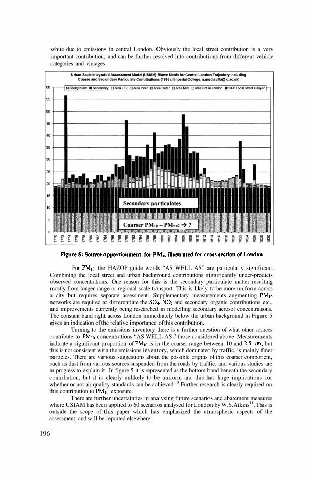
white due to emissions in central London. Obviously the local street contribution is a veryimportant contribution, and can be further resolved into contributions from different vehiclecategories and vintages.
For the HAZOP guide words “AS WELL AS” are particularly significant.Combining the local street and urban background contributions significantly under-predictsobserved concentrations. One reason for this is the secondary particulate matter resultingmostly from longer range or regional scale transport. This is likely to be more uniform acrossa city but requires separate assessment. Supplementary measurements augmentingnetworks are required to differentiate the and secondary organic contributions etc.,and improvements currently being researched in modelling secondary aerosol concentrations.The constant band right across London immediately below the urban background in Figure 5gives an indication of the relative importance of this contribution.
Turning to the emissions inventory there is a further question of what other sourcescontribute to concentrations “AS WELL AS ” those considered above. Measurementsindicate a significant proportion of is in the coarser range between 10 and butthis is not consistent with the emissions inventory, which dominated by traffic, is mainly finerparticles. There are various suggestions about the possible origins of this coarser component,such as dust from various sources suspended from the roads by traffic, and various studies arein progress to explain it. In figure 5 it is represented as the bottom band beneath the secondarycontribution, but it is clearly unlikely to be uniform and this has large implications forwhether or not air quality standards can be achieved.10 Further research is clearly required onthis contribution to exposure.
There are further uncertainties in analysing future scenarios and abatement measureswhere USIAM has been applied to 60 scenarios analysed for London by W.S.Atkins11. This isoutside the scope of this paper which has emphasized the atmospheric aspects of theassessment, and will be reported elsewhere.
196

ConclusionIt is hoped that the two case studies considered above have illustrated how HAZOP
techniques as part of a formal risk assessment, can be useful as a systematic way of examiningmodel functioning and assumptions when used in assessment of air quality problems. Thesetechniques go beyond the traditional methods such as Monte-Carlo analysis, in addressingwhat is not covered in the models as well as questioning the representation andparameterisation of what is included. They point towards potential hazards for the decisionmaker in using the results from a model, and to priority areas for further research. They alsoprovide a framework for linking what are inevitably simplified models in looking at a widerange of possible scenarios in assessing abatement strategies, to a hierarchy of more detailedand sophisticated research concerning the aspects identified. It is suggested that the approachillustrated could usefully provide an appendix to many reports on environmental assessmentbased on numerical models!
AcknowledgmentsThe integrated assessment modelling with ASAM used as case study 1 has been
supported by the UK Department of Environment, Transport and the Regions. The work of AMediavilla-Sahagun on development of the USIAM model in case study 2 has been supportedby the Mexican Petroleum Institute.
References1. CIA (1989) A guide to hazard and operability studies. Chemical Industries Association2. ApSimon HM, Warren RF and Wilson JJN. The Abatement Strategies Assessment Model-ASAM: applications to abatement of sulphur-dioxide emissions across Europe. AtmosphericEnvironment 28(1994)p649-6633. Alcamo J Shaw R and Hordijk L (eds) 1990. The RAINS model of acidification: Scienceand Strategies in Europe. Kluwer Academic Publishers, Dordrecht.4. Warren R F and ApSimon HM (2000). Selection of target loads for acidification inemission abatement policy: the use of gap closure approaches. Water Air and Soil Pollution121, p229-258.5. Warren RF and ApSimon HM (1999) Uncertainties in integrated assessment modelling ofabatement strategies: illustrations with the ASAM model. Environmental Science and Policyvol 2, p439-4566. Warren Rf and ApSimon HM (2001) Integrated Assessment modelling of abatementstrategies: role of uncertainties. Air Pollution Modelling and its Applications XIV,p35-437. ApSimon HM and Warren RF (2001) Addressing uncertainty in environmental modelling;a case study of integrated assessment strategies to combat long-range transboundary airpollution. IUAPPA conference, Korea August 2001.8. Barret K and Seland O (1995) European Transboundary Acidifying Air Pollution. EMEPreport 1/95.9. Kayin S (1993) Wet deposition in convective storms and effects on transboundary airpollution. PhD thesis. University of London.10.Mediavilla-Sahagun A, ApSimon Hm and Warren RF (2001) Integrated Assessment ofAbatement Strategies to Improve Air Quality in London, The USIAM Model. Urban AirQuality conference, Loutraki, Greece, March 2001.11. W S Atkins (1999) An evaluation of transport measures to meet NAQS objectives .Reportto Department of Environment Transport and the Regions.
197
DISCUSSION
B. FISHER
H. APSIMON
A. EBEL
H. APSIMON
198
If one contrasts work undertaken to inform a strategy to controltransfrontier pollution with work on urban pollution, the former wasassociated with extensive testing of models against measurements.The development of strategies for improving urban pollution seem tosuffer from insufficient good quality measurements. Would you liketo comment ?
We have developed integrated assessment modelling along similarlines to analyse strategies to attain air quality standards in London.Here there is quite an extensive monitoring network which we haveused as best we can for model comparison, but limitedmeteorological data-e.g. from Heathrow airport to the west of thecity. The difficulty is the small scale spatial variability even round asingle street junction, and the representativeness of monitoringpoints. As far as PM10 is concerned a substantial correction (~30%)has to be made to the TEOM measurements for loss of the volatilefraction, so care is needed in comparing with model results. Howeverthere are also large problems in modelling such as the coarse PM10-PM2.5 fraction, for which there is no representation in the emissionsinventory. So it is not just the measurements that cause problems inurban assessment, but also the incompleteness of the models andaspects that we do no yet understand. Unfortunately it is not easyconvincing our UK research council that fundamental research anddata are required !
The concept of source-receptor estimates using Lagrangian transportmodelling appears to work reasonably well for “simpler” species like
What is the experience with more complicated chemicals,particularly ozone as a secondary pollutant ?
The illustration I gave in this paper was concerned with sulphur andnitrogen species, where I mentioned the effects of chemistry on non-linear response of concentrations to emissions. We did notspecifically work on ozone in studies for the UN ECE because wewere too occupied with concerns about fine particles. The source-receptor relationships for ozone were produced by IIASA, who fittedempirical quadratic expressions to results from the EMEP model torepresent the response of excess ozone (accumulated above specificconcentration thresholds) to NOx and VOC reductions. A fulluncertainty analysis on this would be complex, but needs to include
P. BUILTJES
H. APSIMON
such factors as trends in background/free troposphere ozone as wellas emission abatement scenarios.
Can you explain why fixing the total costs is more robust thanapproaching the problem from the other angle ?
What seems to be robust is the order of priority of successiveabatement steps selected, based on the ratio of their effectiveness inreducing exceedance to their cost. Even quite large changes in forexample source- receptor matrices, as for example from years withcontrasting meteorology, do not change the order of priority verymuch; nor changes in the critical loads. Hence if one asks what is thestrategy that maximises convergence towards the desired targets orgoals for protection up to a fixed level of costs, this strategy alsotends to be rather robust. However if one aims at strict attainment ofa set of specified target loads for deposition, then usually there areone or two difficult target locations or “binding” grid-cells which aredifficult to achieve. A slight tightening of the targets at theselocations can have big implications for the extra abatement stepsneeded to achieve them and their costs. Effectively this is movingonto the flat part of the curve relating ecosystem protection to cost.Thus sometimes it is apparent that a slight relaxation of such targetsin binding cells avoids some quite large costs.
199

This page intentionally left blank
ETEX SIMULATIONS WITH THE DMI-HIRLAMNUMERICAL WEATHER PREDICTION MODEL
Jérôme Chenevez, Alexander Baklanov and Jens H. Sørensen*
1. INTRODUCTION
Eulerian atmospheric long-range dispersion models to predict air pollution episodesare coupled either offline or online with Numerical Weather Prediction (NWP) models.In the perspective of developing such a mesoscale air pollution forecast system, a versionof the Danish Meteorological Institute’s (DMI) NWP model has been implemented withadvection/diffusion of passive tracers, resulting in the model DMI-HIRLAM-TRACER(shortened as TRACER in the following).
The main objective of this work is to simulate the transport of passive tracers in themodel using the best possible advection scheme. A very suitable and realistic way to testthe advection of a field of passive tracers is supplied by the first European TracerExperiment (ETEX-1) performed in 1994. This release started on October 199416:00 UTC in Brittany (France) and had a duration of 11 hours and 50 minutes. Itsprecise location was (2.0083°W, 48.0583°N) at an altitude of 90 m. The total amount ofmaterial released was 340 kg of Perfluoro-Methyl-Cyclo-Hexane (PMCH) correspondingto a constant emission rate of 7.95 g/sec. The release was followed during 3 days by aseries of measurements of the concentration at specific locations in Europe from which itwas possible to observe the plume evolution (Graziani et al., 1998).
2. SIMULATION OF THE ETEX RELEASE
The present numerical simulations start 4 hours before the beginning of the ETEXrelease by using initial boundary files generated by the European Centre for Medium-Range Weather Forecasts (ECMWF) from October 1994 12:00 UTC. They werecarried out covering more than three days by updating the lateral boundaries every 6
Jérôme Chenevez, Danish Meteorological Institute (DMI), Lyngbyvej 100, 2100 Copenhagen Ø, Denmark.
Air Pollution Modeling and Its Application XV, Edited byBorrego and Schayes, Kluwer Academic/Plenum Publishers, New York, 2002 201
*

202
hours (using 6-hour forecasts and new analysis every 12 hours). The numericalsimulations were performed with TRACER over a model region covering Europe, in agrid with 92×86 points yielding a horizontal resolution of 0.4° (about 42km × 44km); allexperiments were performed using a 31-level resolution in a hybrid vertical coordinatesystem (Sass et al., 2000).
Indications about the performances of these simulations are given by 1) thegeographical position on the surface (more precisely at the lowest model level about 30m above the ground in the present version of TRACER) of the modelled concentrationfield at different forecast times after the start of the release, 2) a time-series of averagedconcentrations at specific model points corresponding to ETEX measurements sites, and3) the evolution of total mass in the model compared to the mass emitted at the releaselocation. The two former outcomes can be compared to real measurements and/or resultsof other models (Graziani et al., 1998; Sørensen et al., 1998, Robertson et al., 1996),while the third allows an evaluation of the stability and the confidence in the schemeused.
Since the conditions of the release are known exactly (location, total mass and rateof release), the main difficulty is to perform such a local release inside an Eulerian gridpoint model. In the present study, a uniform distribution of the tracer is assumed withinthe volume of the grid box inside which the release is initiated. The knowledge of thisvolume makes it possible to calculate the concentration of the passive tracer, in order tocompare the simulated tracer field with the observed concentration field.
The model has to solve the following advection-diffusion equation driving thedynamic evolution of the concentration C of a passive tracer field:
where v represents the advecting velocity vector field, K is a 3 dimensional eddydiffusivity vector, and Q represents the source term.
From the source term of Eq. (1) one can obtain the value at the next time stepof the concentration in the grid box inside which the emission is performed:
That is the concentration of the emitted tracer at the current time step plus theremaining concentration from the previous time step. Hence, during the duration of theemission, the value of the concentration at the point of emission is forced by Eq. (2).

3. TRANSPORT USING DMI-HIRLAM DEFAULT SETUP
Simulations of the ETEX release have first been performed using the default DMI-HIRLAM formulation of Eq. (1) for a scalar. In this formulation, advection is describedby the Eulerian central finite-difference scheme in a semi-implicit time scheme wherenegative values of positive definite quantities are set to zero so as to avoid unrealisticnegative concentrations; the consequences of such a resetting procedure will bediscussed later. Horizontal diffusion processes, on the one hand, are estimated by animplicit linear order scheme (Källen, 1996), and vertical diffusion, on the other, iscomputed by a local turbulent kinetic energy scheme known as the CBR method (Cuxartet al., 1999).
Modelled surface concentration at 48 hours after the start of the release is shown onFigure 1 in a zoom inside the model domain. The general shape and position of theplume are rather close to the observations made during the experiment (Graziani et al.,1998), though physical diffusion seems to be too large.
Figure 2 compares measured and modelled one-hour average surface concentrationsat the location of Risø (Denmark). The time of the peak is fairly well predicted, but itsvalue is more than twice the observed value, and the shape of the curve is too wide dueto diffusion and low grid resolution.
The reason for this too high value is shown on Figure 3, which presents theevolution of the mass of passive tracers relative to the total mass released. The curveobtained with the central difference scheme shows an increase in the amount of passivetracers of more than 1.5 times the total mass emitted, indicating that mass is notconserved during the simulation. Indeed, the mass continues to increase linearly evenafter the emission phase, thus showing an artificial production of mass in the model.
203

204
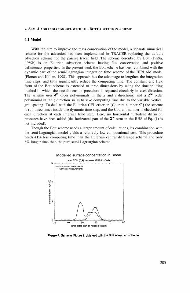
4. SEMI-LAGRANGIAN MODEL WITH THE BOTT ADVECTION SCHEME
4.1 Model
With the aim to improve the mass conservation of the model, a separate numericalscheme for the advection has been implemented in TRACER replacing the defaultadvection scheme for the passive tracer field. The scheme described by Bott (1989a,1989b) is an Eulerian advection scheme having flux conservation and positivedefiniteness properties. In the present work the Bott scheme has been combined with thedynamic part of the semi-Lagrangian integration time scheme of the HIRLAM model(Ekman and Källen, 1998). This approach has the advantage to lengthen the integrationtime steps, and thus significantly reduce the computing time. The constant grid fluxform of the Bott scheme is extended to three dimensions by using the time-splittingmethod in which the one dimension procedure is repeated circularly in each direction.The scheme uses order polynomials in the x and y directions, and a orderpolynomial in the z direction so as to save computing time due to the variable verticalgrid spacing. To deal with the Eulerian CFL criterion (Courant number the schemeis run three times inside one dynamic time step, and the Courant number is checked foreach direction at each internal time step. Here, no horizontal turbulent diffusionprocesses have been added (the horizontal part of the term in the RHS of Eq. (1) isnot included).
Though the Bott scheme needs a larger amount of calculations, its combination withthe semi-Lagrangian model yields a relatively low computational cost. This procedureneeds 41% less computing time than the Eulerian central difference scheme and only8% longer time than the pure semi-Lagrangian scheme.
205
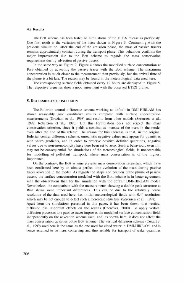
4.2 Results
The Bott scheme has been tested on simulations of the ETEX release as previously.One first result is the variation of the mass shown in Figure 3. Contrasting with theprevious simulation, after the end of the emission phase, the mass of passive tracersremains approximately constant during the transport phase. This behaviour confirms themajor improvement due to the Bott scheme as regards the mass conservationrequirement during advection of passive tracers.
In the same way as Figure 2, Figure 4 shows the modelled surface concentration atRisø obtained by advecting the passive tracer with the Bott scheme. The maximumconcentration is much closer to the measurement than previously, but the arrival time ofthe plume is a bit late. The reason may be found in the meteorological data used here.
The corresponding surface fields obtained every 12 hours are displayed in Figure 5.The respective vignettes show a good agreement with the observed ETEX plume.
5. DISCUSSION AND CONCLUSION
The Eulerian central difference scheme working as default in DMI-HIRLAM hasshown reasonably good qualitative results compared with surface concentrationmeasurements (Graziani et al., 1998) and results from other models (Sørensen et al.,1998; Robertson et al., 1996). But this formulation does not respect the massconservation criterion, since it yields a continuous increase of the mass in the modeleven after the end of the release. The reason for this increase is that, in the originalEulerian central difference scheme, unrealistic negative values may appear for quantitieswith sharp gradients, and in order to preserve positive definite quantities, negativevalues due to non-monotonicity have here been set to zero. Such a behaviour, even if itmay not be consequential for simulations of the meteorological fields, is unacceptablefor modelling of pollutant transport, where mass conservation is of the highestimportance.
On the contrary, the Bott scheme presents mass conservation properties, which havebeen confirmed here by an almost perfect time evolution of the mass during passivetracer advection in the model. As regards the shape and position of the plume of passivetracers, the surface concentration modelled with the Bott scheme is in better agreementwith the observations than for the simulation with the default DMI-HIRLAM model.Nevertheless, the comparison with the measurements showing a double-peak structure atRisø shows some important differences. This can be due to the relatively coarseresolution of the data used here, i.e. initial meteorological fields with 0.4° resolution,which may be not enough to detect such a mesoscale structure (Sørensen et al., 1998).Apart from the simulations presented in this paper, it has been shown that verticaldiffusion has important effects on the results (Chenevez, 2000). To apply verticaldiffusion processes to a passive tracer improves the modelled surface concentration field,independently on the advection scheme used, and, as shown here, it does not affect themass conservation qualities of the Bott scheme. The vertical diffusion scheme (Cuxart etal., 1999) used here is the same as the one used for cloud water in DMI-HIRLAM, and ishence assumed to be mass conserving and thus reliable for transport of scalar quantities
206
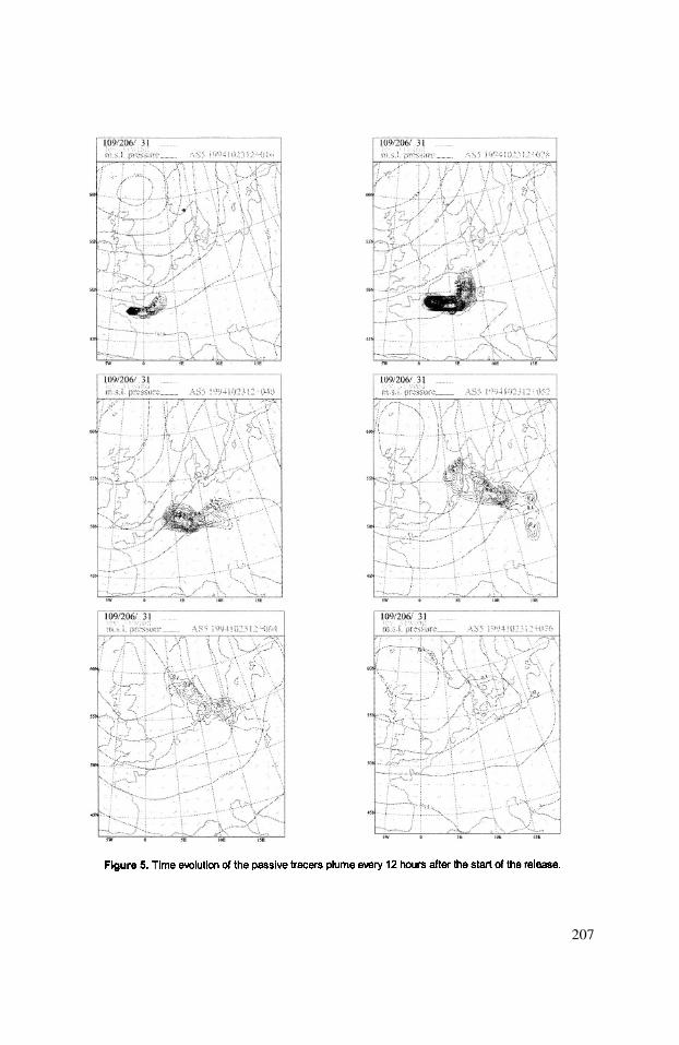
207

like chemical constituents and any other pollutants. It has also been shown in the samework that using a order horizontal diffusion scheme (Mc Donald, 1994) together withthe Bott scheme corrupts its mass conservation properties. This may be due either to apoor formulation of the horizontal turbulence processes, or to some incompatibilitiesbetween the diffusion scheme and the Bott scheme during the splitting step. It is thuspreferable at this stage to avoid adding the term of horizontal diffusion in thesimulations with the Bott scheme, unless it is formulated in a way that compensates forthe numerical diffusion inherent to the Bott scheme.
One of the principal outcomes of this work is that the Bott scheme used inside thesemi-Lagrangian model yields only 1.08 longer computation time than the semi-Lagrangian scheme alone, and it is even 1.6 times as faster as the Eulerian centraldifference scheme. Better results are thus obtained in a shorter time than with thedefault setting of DMI-HIRLAM.
In conclusion, the present simulation tests have shown that, when including a massconservative advection scheme together with vertical diffusion processes for the passivetracers, the TRACER model can be used for transport modelling.
ACKNOWLEDGEMENTS
The authors are grateful to Annica Ekman from MISU who have supplied the codeof the Bott scheme. Thanks to Leif Laursen, Bennert Machenhauer and Xiang-YuHuang for their critical reading of the manuscript, and also to Jess U. Jørgensen, BentHansen Sass, and Niels Woetmann Nielsen for their helpful advice.
REFERENCES
Bott, A., 1989a, A positive definite advection scheme obtained by non-linear renormalization of the advectivefluxes, Mon. Wea. Rev. 117: 1006-1015.
Bott, A., 1989b, Reply, Mon. Wea. Rev., 117: 2633-2636.Chenevez, J., 2000, Advection experiments with DMI-HIRLAM-TRACER. DMI Scientific Report 00-05;
http://www.dmi.dk/f+u/publikation/vidrap/2000/Sr00-05.pdf.Cuxart, J., Bougeault, P., and Redelsperger, J.-L., 1999, A turbulence scheme allowing for mesoscale and large
eddy simulations, Q. J. R. Meteorol. Soc. XXX: 1-22.Ekman, A. and Källen. E., 1998, Mass conservation tests with the HIRLAM semi-Lagrangian time integration
scheme, HIRLAM Technical Report N°39, Dublin, Ireland.Graziani, G., Klug, W., and Mosca, S., 1998, Real-Time Long-Range Dispersion Model Evaluation of the ETEX
first Release, Office for Official Pub. of the European Communities, Luxembourg, EUR 17754 EN.Källen, E., 1996, “HIRLAM documentation manual, System 2.5”, SMHI, Norrköping, Sweden.McDonald A., 1994, The HIRLAM two time level, three dimensional semi-Lagrangian, semi-implicit, limited area,
grid point model of the primitive equations, HIRLAM Technical Report N°17, Norrköping, Sweden.Robertson, L., Langner, J., and Engardt, M., 1996, MATCH - Meso-scale Atmospheric Transport and Chemistry
modelling system, SMHI Reports Meteorology and Climatology N° 70.Sass, B. H., Nielsen, N. W., Jørgensen, J.U., Amstrup, B., and Kmit, M., 2000, The operational HIRLAM system,
DMI Technical report 00-26. http://www.dmi.dk/f+u/publikation/tekrap/2000/Tr00-26.pdf.Sørensen, J.H., Rasmussen, A., Ellermann, T., and Lyck, E., 1998, Mesoscale influence on long-range transport -
Evidence from ETEX modelling and observations, Atmos. Env.32: 4207-4217.
208

DISCUSSION
S.E. GRYNING
J. CHENEVEZ
The prediction of the time of arrival of the tracer plume is not sowell predicted in your simulations as in earlier simulations done atthe Danish Meteorological Institute by J.H. SØRENSEN (specialETEX issue on Atmospheric Environment). Do you have anysuggestions for an explanation ?
We are speaking about two different kinds of models: J. H.Sørensen’s model DERMA is based on a Lagrangian transportmodel, while DMI-HIRLAM is an Eulerian model. However,according to J. H. Sørensen’s work, DERMA gave approximately thesame results when used with the same model resolution as in thepresent work, while better results were only obtained with a highermodel resolution, showing that a mesoscale structure influenced thetracer plume about one day before arriving to Risø.Another possible cause of the delay obtained in the modelled peaksmay be slide phase errors of the version of the Bott advectionscheme employed here, as noticed by Bott himself and corrected in afurther version, which we still have to implement.
209

This page intentionally left blank

IMPACT ASSESSMENT OF GROWING ASIANMEGACITY EMISSIONS
Sarath K. Guttikunda, James J. Yienger, Narisara Thongboonchoo,Gregory R. Carmichael, Hiram Levy II and David G. Streets*
1. INTRODUCTION
The urban environment is where an increasing share of the world’s people live,where most of the energy is consumed, and where the impacts of the pollution are felt themost. While the effects of high pollution levels in Asia are centered in the urban areas,the impacts are not confined to the city boundaries. Polluted air has damaged humanhealth, ecology and environment in a number of urban centers of the developing countriesof Asia. Most of the air pollution is emitted by stationary sources like power plants andindustrial estates. Pollution from the mobile sources volatile organic carbons(VOC) and particulates) has become a major contributor to increasing human healtheffects in the urban environments of Asia (OECD, 2000).
Rapid economic growth in Asia over several decades has attracted millions ofrural residents to urban areas. Figure 1 presents gridded Asian population for 2000 alongwith Asian megacities (with population over 10 million) and major urban centers. Asiapresently has ~1 billion (~35% of total population) urban dwellers, projected to grow atan average of 4% per year to ~3 billion by 2025 (~55% of the projected total population).Changing standards of living in these centers have fueled increased industrial andtransportation sector activities, often associated with unchecked emissions fromautomobiles, domestic heating, and small-scale industries. Coal (besides bio-fuel (wood,cow dung, and field residue)) being the cheapest and most widely available source ofenergy, still remains the primary source of energy, and contributes significantly to sulfur
Sarath Guttikunda, Narisara Thongboonchoo, and Gregory Carmichael (corresponding author,[email protected]), Department of Chemical and Biochemical Engineering, The University ofIowa, Iowa City, IA 52242, USA. James Yienger, Center for Global and Regional Environmental Research,The University of Iowa, Iowa City, IA, USA. Hiram Levy II, Geophysical Fluid Dynamic Laboratories,Princeton University, NJ, USA. David Streets, Argonne National Laboratories, Argonne, IL, USA.
Air Pollution Modeling and Its Application XV, Edited byBorrego and Schayes, Kluwer Academic/Plenum Publishers, New York, 2002 211
*
and particulate concentrations often exceeding the WHO air quality guidelines. Increaseduse of biofuels, especially in the rural regions of the developing countries, pose severehuman health concerns due to increased particulate pollution both indoors and outdoors.Every year, Asian urban centers prone to air pollution incur hundreds of millions ofdollars in health and economic damages (OECD, 2000). Presently, the urban air pollutionproblems in Asia are continuing to increase and air pollutants originating from urbanregions are now recognized as increasing sources of regional- and global-scale pollution(Streets et al., 1999).
This study is an effort to understand the nature of growing emissions from theurban centers of Asia, to characterize the impact of these emissions on trace gas speciesat urban and regional scale. And finally, to evaluate costs and benefits of implementingemission reduction techniques for sulfur, particulates and for Asian megacities.
2. MEGACITY EMISSIONS
Emissions of and were estimated through the establishment ofemission factors (emissions per unit of energy consumption) by energy source and bysector of energy use, as part of the RAINS-Asia project (Arndt et al., 1997 and vanAardenne et al., 1999). In the case of “business as usual” energy consumption, theprojections show an increase of and emissions in the Asian region in 2020 to 2-3 times the levels of 1990 (Foell et al., 1995 and van Aardenne et al., 1999). The fact thatthe megacities and urban centers in Asia cover less than 1% of the landcover and stillproduce 10-20% of trace gas emissions signifies their importance.
LandScan 2000, Global Population at 30 Arc Second Grid, developed by Oak Ridge National Laboratory,United States Department of Defense, March 2001.
212
1
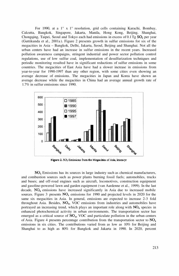
For 1990, at a 1° x 1° resolution, grid cells containing Karachi, Bombay,Calcutta, Bangkok, Singapore, Jakarta, Manila, Hong Kong, Beijing, Shanghai,Chongqing, Taipei, Seoul and Tokyo each had emissions in excess of 0.1 Tg per year(Guttikunda et al., 2001a ). Figure 2 presents growth in sulfur emissions for six of themegacities in Asia – Bangkok, Delhi, Jakarta, Seoul, Beijing and Shanghai. Not all theurban centers have had an increase in sulfur emissions in the recent years. Increasedpollution awareness campaigns, stringent industrial and power sector pollution controlregulations, use of low sulfur coal, implementation of desulfurization techniques andperiodic monitoring resulted have in significant reductions of sulfur emissions in somecountries. The megacities of East Asia have had a slower increase in emissions fromyear-to-year for 1990-1997 than any other region, with some cities even showing anaverage decrease of emissions. The megacities in Japan and Korea have shown anaverage decrease while the megacities in China had an average annual growth rate of1.7% in sulfur emissions since 1990.
Emissions has its sources in large industry such as chemical manufacturers,and combustion sources such as power plants burning fossil fuels; automobiles, trucksand buses; and off-road engines such as aircraft, locomotives, construction equipmentand gasoline-powered lawn and garden equipment (van Aardenne et al., 1999). In the lastdecade, emissions have increased significantly in Asia due to increased mobilesources. Figure 3 presents emissions for 1990 and projected levels in 2020 for thesame six megacities in Asia. In general, emissions are expected to increase 2-3 foldthroughout Asia. Besides, VOC emissions from industries and automobiles haveportrayed an increasing trend, which plays an important role along with species inenhanced photochemical activity in urban environments. The transportation sector hasemerged as a critical source of VOC and particulate pollution in the urban centersof Asia. Figure 4 presents percentage contribution from the transportation sector toemissions in six cities. The contributions varied from as low as 10% for Beijing andShanghai to as high as 80% for Bangkok and Jakarta in 1990. In 2020, percent
213
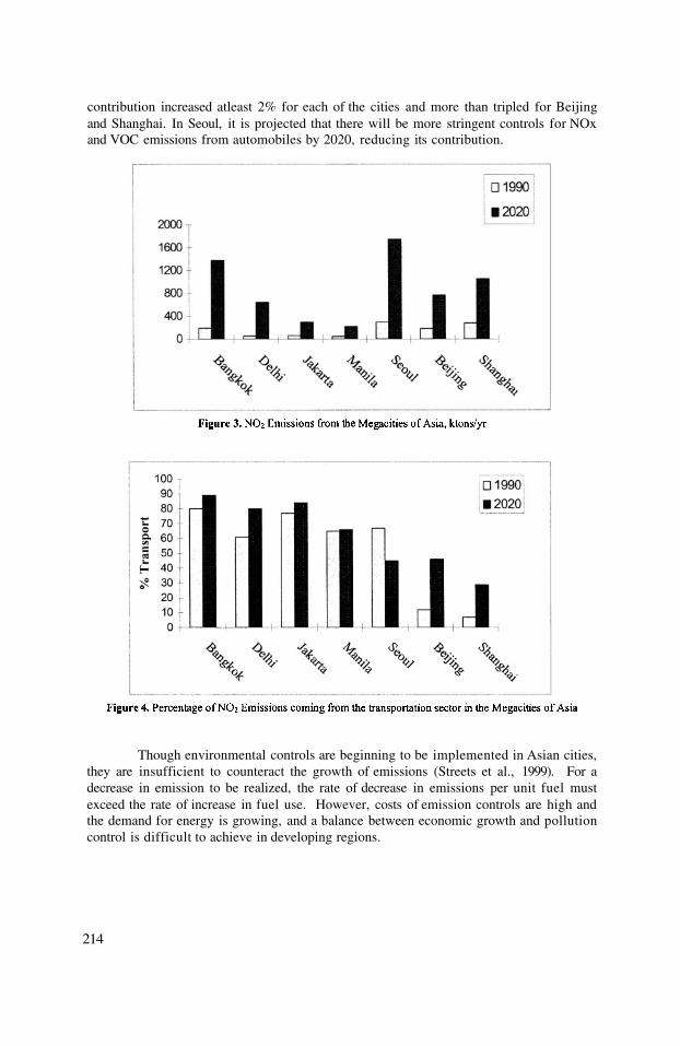
contribution increased atleast 2% for each of the cities and more than tripled for Beijingand Shanghai. In Seoul, it is projected that there will be more stringent controls for NOxand VOC emissions from automobiles by 2020, reducing its contribution.
Though environmental controls are beginning to be implemented in Asian cities,they are insufficient to counteract the growth of emissions (Streets et al., 1999). For adecrease in emission to be realized, the rate of decrease in emissions per unit fuel mustexceed the rate of increase in fuel use. However, costs of emission controls are high andthe demand for energy is growing, and a balance between economic growth and pollutioncontrol is difficult to achieve in developing regions.
214
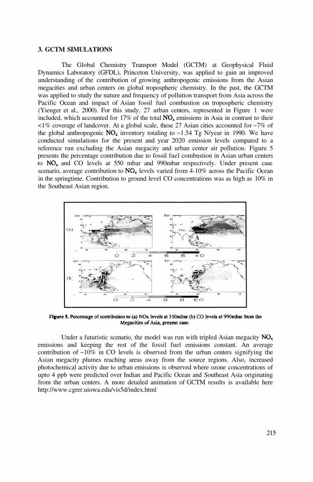
3. GCTM SIMULATIONS
The Global Chemistry Transport Model (GCTM) at Geophysical FluidDynamics Laboratory (GFDL), Princeton University, was applied to gain an improvedunderstanding of the contribution of growing anthropogenic emissions from the Asianmegacities and urban centers on global tropospheric chemistry. In the past, the GCTMwas applied to study the nature and frequency of pollution transport from Asia across thePacific Ocean and impact of Asian fossil fuel combustion on tropospheric chemistry(Yienger et al., 2000). For this study, 27 urban centers, represented in Figure 1 wereincluded, which accounted for 17% of the total emissions in Asia in contrast to their<1% coverage of landcover. At a global scale, these 27 Asian cities accounted for ~7% ofthe global anthropogenic inventory totaling to ~1.54 Tg N/year in 1990. We haveconducted simulations for the present and year 2020 emission levels compared to areference run excluding the Asian megacity and urban center air pollution. Figure 5presents the percentage contribution due to fossil fuel combustion in Asian urban centersto and CO levels at 550 mbar and 990mbar respectively. Under present casescenario, average contribution to levels varied from 4-10% across the Pacific Oceanin the springtime. Contribution to ground level CO concentrations was as high as 10% inthe Southeast Asian region.
Under a futuristic scenario, the model was run with tripled Asian megacityemissions and keeping the rest of the fossil fuel emissions constant. An averagecontribution of ~10% in CO levels is observed from the urban centers signifying theAsian megacity plumes reaching areas away from the source regions. Also, increasedphotochemical activity due to urban emissions is observed where ozone concentrations ofupto 4 ppb were predicted over Indian and Pacific Ocean and Southeast Asia originatingfrom the urban centers. A more detailed animation of GCTM results is available herehttp://www.cgrer.uiowa.edu/vis5d/index.html
215

4. INTEGRATED ASSESSMENT OF URBAN AIR QUALITY
Global and Regional scale long-transport models play a critical role inunderstanding the transport and chemical transformation of trace gas species andparticulates. Long range transport models also play a key role in environmentalmanagement, in that they link emissions to concentrations, and thus are used to evaluatethe impact of emerging energy policies and to analyze the environmental and healtheffects and the economic benefits of emission abatement options for reducingVOC and particulate matter emissions. The management of emissions in Asia megacitiesrequires a better understanding on emission sources, distribution and their controls. Forthis study we developed a conceptual Integrated Assessment Modeling System (IAMS),for Asian megacities, which provides a methodology for identifying interactions betweenenvironmental drivers (pollutant concentrations and depositions) and endpoints likehuman health, environmental and structural damage (Guttikunda et al, 2001b).
In continuing support of the integrated assessment modeling of air pollution inAsia, which started as part of the RAINS-Asia (Regional Air pollution INtegration andSimulation – Asia) project, the analysis of air quality management studies are extended toinclude particulates and megacities of Asian developing countries. Figure 6 presents anoutline of the modeling system. IAMS has a similar structural framework as RAINS butfocuses more on the urban air quality management. Model framework includes a grid-to-grid transfer matrix (generated using lagrangian puff transport model, ATMOS (Arndt,1997)) for sulfur and particulate concentration and deposition, combined with health andenvironmental damage assessment and cost-benefit analysis. The framework can beadapted to any urban area of interest enabling a) dispersion modeling of sulfur andparticulates b) quantifying costs and benefits of available control strategies c) assessingeffects of possible change in energy end-use patterns, technology changes d) assessment
216
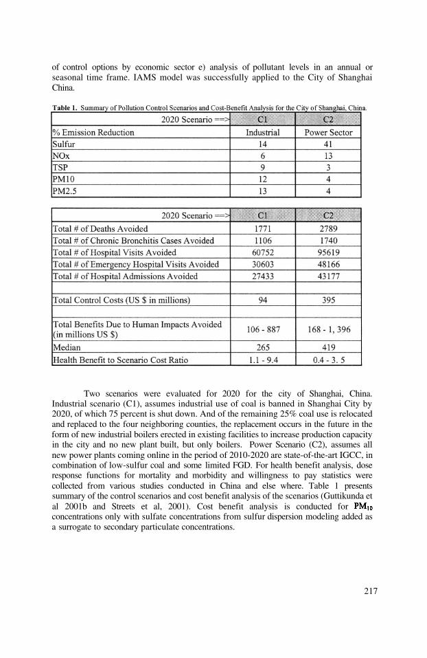
of control options by economic sector e) analysis of pollutant levels in an annual orseasonal time frame. IAMS model was successfully applied to the City of ShanghaiChina.
Two scenarios were evaluated for 2020 for the city of Shanghai, China.Industrial scenario (C1), assumes industrial use of coal is banned in Shanghai City by2020, of which 75 percent is shut down. And of the remaining 25% coal use is relocatedand replaced to the four neighboring counties, the replacement occurs in the future in theform of new industrial boilers erected in existing facilities to increase production capacityin the city and no new plant built, but only boilers. Power Scenario (C2), assumes allnew power plants coming online in the period of 2010-2020 are state-of-the-art IGCC, incombination of low-sulfur coal and some limited FGD. For health benefit analysis, doseresponse functions for mortality and morbidity and willingness to pay statistics werecollected from various studies conducted in China and else where. Table 1 presentssummary of the control scenarios and cost benefit analysis of the scenarios (Guttikunda etal 2001b and Streets et al, 2001). Cost benefit analysis is conducted forconcentrations only with sulfate concentrations from sulfur dispersion modeling added asa surrogate to secondary particulate concentrations.
217
5. CONCLUSIONS
Urban air pollution in Asia has worsened in the developing countries, a situationdriven by population growth, industrialization, and increased vehicle use. With anestimated 3 billion (~55%) urban residents in Asia in 2025 in <5% of the Asia’s landcover and human health effects as a primary measure urban environments are the first toreact to any of the pollution control regulations. Modeling activities were conducted tounderstand and characterize the urban air pollution in Asia at local, regional and globalscales. GFDL/GCTM simulations under two scenarios were conducted to establish theimpact of growing emissions on regional photochemical activity where contributionsof >10% for CO and at ground level were predicted. Given the growing importanceof urban air quality management, we have applied a conceptual integrated assessmentmodeling system to conduct cost-health benefit analysis for various pollution controloptions in the city of Shanghai, China. IAMS was applied for ground levelconcentrations with sulfate concentrations as a surrogate for secondary particulates. Infuture, we would like to conduct integrated assessment including other secondarycomponents like nitrates, and secondary organic aerosols. Further advancements inmodeling activities like nested grid analysis, will help better understand and manage theurban air quality whose influence on regional and global air quality is growing more thanever.
6. REFERENCES
Arndt, R., 1997, The Role of Sulfur Emissions in Asia’s Environmental Change: Analysis on a Regional andUrban Scale, Ph. D thesis, The University of Iowa, USA.
Arndt, R. L., Carmichael, G. R., Streets, D. G., and Bhatti, N., 1997, Sulfur dioxide emissions and sectorialcontributions to sulfur deposition in Asia’, Atmos. Env., 31, 1553.
Foell, W., Green, C., Amann, M., Bhattacharya, S., Carmichael, G., Chadwick, M., Cinderby, S., Haugland, T.,Hettelingh, J.-P., Hordijk, L., Kuylenstierna, J., Shah, J., Sherestha, R., Streets, D., Zhao, D., 1995,Energy use, emissions, and air pollution reduction strategies in Asia, Water, A ir, and Soil Pollut, 85, 2277.
Guttikunda, S. K., Thongboonchoo, N., Arndt, R. L., Calori, G., Carmichael, G. R., and Streets, D. G., 2001a,Sulfur deposition in Asia: Seasonal behavior and contributions from various energy sectors, Water, Airand Soil Pollut, 131, 383.
Guttikunda, S. K., Carmichael, G. R., Streets, D. G., and Amann , M., 2001b, An integrated assessmentmodeling system (IAMS) for sulfur and paniculate air pollution in the megacities of Asia, Technicalreport submitted to International Institute of Applied Systems Analysis (IIASA), Laxenburg, Austria.
OECD, 2000, Ancillary Benefits and Costs of Greenhouse Gas Mitigation, Proceedings of an IPCC Co-sponsored workshop, 27-29 March 2000, in Washington DC, USA.
Streets, D. G., Carmichael, G. R., Amann, M. and Arndt, R. L., 1999, Energy consumption and acid depositionin northeast Asia, Ambio, 28, 135.
Streets, D. G., Guttikunda, S. K., Li, J., Chang, Y-S., Carmichael, and G. R., 2001, Integrated assessment of airquality impacts in Asian cities: and Particulate Matter in Shanghai., In preparation,
van Aardenne, J. A., Carmichael, G. R., Levy, H., Streets, D. G., and Hordijk, L., 1999, Anthropogenicemissions in Asia in the period 1990-2020, Atmos Env, 33, 633.
Yienger, J. J., Galanter, M. K., Holloway, T. A., Phadnis, M. J., Guttikunda, S. K., Carmichael, G. R., Moxim,W. J., and Levy, H., II, 2000, The frequency and nature of air pollution transport from Asia to NorthAmerica, J of Geophy. Res., 105, 26, 931.
218

DISCUSSION
A. HANSEN
S. GUTTIKUNDA
Although your integrated analysis shows promise, I would take issuewith the health benefits associated with reductions in particulatesulfate, since epidemiological studies of associations betweencomponents of PM10 or PM2.5 and mobility and mortality show noincreased risk associated with sulfate.
I agree that mortality and morbidity show less increased associationwith sulfate concentrations alone, but chemical composition ofPM2.5 and PM10 in Asian cities, especially in cities like Shanghai,Seoul have shown that the secondary particulate concentration in theform of sulfate and nitrate is significantly high which in turn promptsus to look into combinedimplications of controlling particulate,Sulfur and NOx emissions.
219

This page intentionally left blank

TRANSBOUNDARY EXCHANGE OF SULFURPOLLUTION IN THE REGION OF SE EUROPE
Dimiter Syrakov, Maria Prodanova*
1. INTRODUCTION
The Co-operative Programme for Monitoring and Evaluation of the Long-Range Trans-mission of Air pollutants in Europe (EMEP) was lunched to serve the Convention onLong Range Transboundary Air Pollution. This convention, signed in 1979, is one of thecentral means for protection of our environment. It establishes a broad framework for co-operative action on reducing the impact of air pollution and sets up a process for negotiat-ing concrete measures to control emissions of air pollutants through legally binding pro-tocols. The main objective of the EMEP programme to is to regularly provide partiesunder the Convention with qualified scientific information. EMEP have three main tasks:(1) collection of emission data, (2) measurements of air and precipitation quality and (3)modeling of transport and deposition of air pollution. Three main bodies are establishedfor their implementation. The co-ordination and intercallibration of chemical air qualityand precipitation measurements are carried out at the Chemical Coordinating Centre(CCC). The storage and distribution of reliable information on emissions is the duty of theMeteorological Synthesizing Centre-West (MSC-W). The MSC-W is also responsible forthe modeling assessment of acid and photooxidant pollutants. The modeling developmentfor heavy metals and POPs is responsibility of the Meteorological Synthesizing Centre-East (MSC-E). Initially, all model estimates were performed for a grid with 150-km stepcovering mainly Europe. Last years the region was enlarged and the resolution was im-proved to 50 km.
In this paper the EMEP methodology for estimating the exchange of pollution be-tween countries is applied on finer grid for the region of southeastern Europe. A modelcalled EMAP is used to estimate the sulfur deposition over Balkan peninsula for 1995 dueto Bulgarian and Greek sources. As only sources over these two countries are handled the
Dimitar Syrakov, Maria Prodanova, National Institute of Meteorology and Hydrology, Bulgarian Academy
of Sciences, Sofia, Bulgaria.
Air Pollution Modeling and Its Application XV, Edited byBorrego and Schayes, Kluwer Academic/Plenum Publishers, New York, 2002 221

results can be considered as an estimate of Bulgarian and Greek impact in the acid pollu-tion of the region as well as an estimate of the reciprocal pollution.
SHORT DESCRIPTION OF EMAP MODEL
EMAP (Eulerian Model for Air Pollution) is a 3D simulation model, which allowsdescribing the dispersion of multiple pollutants (BC-EMEP 1994-1997; Syrakov 1995,1997b). The processes as horizontal and vertical advection, horizontal and vertical diffu-sion, dry deposition, wet removal, gravitational settling (aerosol version) and simplestchemical transformation (sulfur version) are accounted for. Within EMAP, the semi-empirical diffusion-advection equations for scalar quantities are treated. The governingequations are solved in terrain-following coordinates. Non-equidistant grid spacing is set-tled in vertical directions. The numerical solution is based on discretization applied onstaggered grids. Conservative properties are fully preserved within the discrete modelequations.
Advective terms are treated with a Bott-type scheme called TRAP (Syrakov 1996,1997a; Syrakov and Galperin 1997b). Displaying the same simulation properties as theBott scheme (explicit, conservative, positively definite, transportive, limited numericaldispersion) the TRAP scheme occurs to be several times faster. The advective boundaryconditions are zero at income flows and “open boundary” - at outcome ones. Turbulentdiffusion equations are digitized by means of the simplest schemes - explicit in horizontaland implicit in vertical direction. The bottom boundary condition for the vertical diffusionequation is the dry deposition flux; the top boundary condition is optionally “open bound-ary” and “hard lid” type. The lateral boundary conditions for diffusion are “open bound-ary” type. In the surface layer (SL), a parameterization is applied permitting to have thefirst computational level at the top of SL. It provides a good estimate for the roughnesslevel concentration and accounts also for the action of continuous sources on the earthsurface (Syrakov and Yordanov 1997). The simplest decay approach is applied for wetremoval, coefficient depending on pollutant properties and on rain intensity. The gravita-tional settling and the wet removal of pollutants carried by aerosols are described on thebase of Galperin’s parameterization (Syrakov and Galperin 1997a).The emissions are provided in mass units per second. For the high sources called LargePoint Sources (LPS) {i, j, h, strength} is necessary, for the area sources (ARS) {i, j,strength} is required.
Only 850 hPa U-, V- and as well as surface are necessary as meteoro-logical input, being potential temperature. A simple PBL model (Yordanov et al. 1983)is built in EMAP producing U-, V-, W- and at each grid point. It provides also
and SL universal profiles needed by the SL parameterization scheme.EMAP model was validated in the frame of ETEX-II study: it was ranged 9th among 34models (Syrakov and Prodanova 1997). It was also validated in EMEP/MSC-E intercali-brations of heavy metal models (Syrakov and Galperin 1997a; Gussev et al. 2000).
222

3. SULFUR PARAMETERIZATION AND MODEL PARAMETERS
Here, the simplest sulfur model is used. Two airborne species of sulfur are consid-ered - gaseous sulfur dioxide and particulate sulfate The sources emitonly. In the air is transformed to sulfate with constant transformation ratefor winter and for summer. Both species are objects of dry and wet removal.The dry deposition velocity for is set to over land and overseas. For these values are 0.02 and 0.06 m/s, respectively. The wet removal con-stant is set to for and for
4. MODEL DOMAIN AND INPUT FIELDS
The aim of this modeling is to estimate the sulfur pollution in the region of southeast-ern Europe, taking a territory of 8x9 EMEP’s grid cells with Bulgaria in thecenter. Every cell is divided to 36 cells. The chosen territory includes entirelyAlbania (ALB), Bulgaria (BUL), Moldova (MOL) and Marmara sea (MRS), almost allGreece (GRE) - only the most southern islands are out domain, parts of Romania (ROM),Turkey (TUR), Yugoslavia (YUG), Ukraine (UKR), Black (BLS), Adriatic (ADS) andAegean (AES) seas. In the applied version of EMAP, a 5-layer structure is used. The firstfour layers have representative levels at 50, 200, 650 and 1450 m with layer boundaries20-100, 100-375, 375-995, 995-1930 m. The 5th layer accounts parameterically for thefree atmosphere. In spite it can contain some mass, the volume of this layer is so big thatthe concentration tends to be zero, there.
Two kinds of input are necessary for EMAP performance - emissions (source input)and meteorology.
223

4.1. Source Input.
The sources are determined through emission inventory based on the CORINAIRmethodology. The sources of Bulgaria are shown in Fig.1.
They correspond to the official data reported to EMEP/MSC-W by Bul-garian authorities. Additional redistribution of this data is made over the finer grid of 25km step. The most powerful source in the country is “Maritsa Iztok” - a set of 3 neighbor-ing coal firing thermal power plants. They are so close to each other that occupy three 25km cells, their total emission rate estimated to 17.15 kg sulfur per second. The othersources are rather small in comparison with these ones. As all LPS are supplied with highstacks, the emission of these sources is prescribed to be released in layer 2, i.e. between100 and 375 m. The total amount of sulfur emission of Bulgaria for 1995 is estimated to748.6 kt S (kilotons); 651.14 kt S due to large point sources and 97.5 kt S - to areasources.
The information of Greek sources for 1995 is provided by European EnvironmentalAgency and EMEP/MSC-W as official data in 50 km resolution. Here, only simple divid-ing of every cell to 4 cells is made, space distribution shown in Fig.2. The to-tal sulfur emission of Greece for 1995 is estimated to 304.7 kt S. The amount released bylarge point sources is 179.3 kt S and by area sources -125.4 kt S.
As polluters, both countries have almost equal intensity (as order of magnitude), butthe structure of sources is very different. 85% of Bulgarian sulfur emission is due to LPS(mainly “Maritsa-Iztok” TPP) while in Greece the emission is divided between the twokinds of sources. Bulgarian release is more than twice the Greek one; the Greek areasources emit more sulfur than Bulgarian ones. All this peculiarities together with theweather character during this particular year determine the way of exchange of sulfur pol-lution between Bulgaria and Greece.
224

The meteorology input has time resolution of 6 hours. It consists of sequence of ana-lyzed and fields and 6-hour forecast for precipitation. The standard
output of the “Europa-Model” of Deutscher Wetterdienst, Offenbach, Ger-many, distributed via the GTS of the WMO is used here.
Annual runs with Bulgarian and Greek sources are performed. As the calculations aremade month by month, the current concentrations at the end of one month integration isinput as initial field for the next month. The initial concentration for the first month of theyear is obtained by integration over some final days of previous month or by spin-up pro-cedure using the first days of the current month. The following fields are the final output:annual dry (DD), wet (WD) and total (TD) depositions, mean annual concentration in air(CA) and mean annual concentration in precipitation (CP).
225
4.2. Meteorology Input
5. CALCULATION RESULTS
5.1. Comparison with Measurements
Very few measurement data are available as to validate the calculation results. Thereis not any EMEP station in the region. For some period of time a background station ofBulgarian Ministry of Environment used to operate in the National Astronomic Observa-tory “Rojen”. It is placed on a peak with 1800 m height in the Rhodopy Mountains, situ-ated both in Bulgaria and in Greece. It must be noticed that the observation methodologywas not very precise for background purposes, but the results can be used for comparisonat least as order of magnitude. Here, the graphical data given in “Status of the environ-ment of Republic of Bulgaria - 1995”, Bulletin of the National Center of Environment andSustainable Development at the Ministry of Environment, page 92. Only mean monthly
and concentrations are presented there. In Fig.3, the measured and calculatedmonthly and annual concentrations are presented together.

The space distributions of the annual concentration in air and in precipitation due toBulgarian sulfur sources for 1995 show that the maximums are in the region of the mostpowerful thermal power plants “Maritsa-Iztok”. A secondary maximum is observed overthe region of Sofia. The impact of Bulgarian sources in pollution over Greece is rela-tively high. Over northern Greece the concentration levels are about one order of magni-tude less than the maximums and concentrations over the other part of Greece are 1.5-2orders less then the maximum.
The total deposition of sulfur oxides due to Bulgarian sources is shown in Fig.4a andthe distribution of these loads between the different territories, listed in the beginning ofpart 4, is displayed in Table 1, where the month-by-month variations can be seen, too.The last row and column in the table show the percentage of deposed quantities from thereleased one. It can be seen that about 27% from the Bulgaria emitted sulfur are depositedover the country itself; other 27% are deposited in the neighborhood; the rest goes out ofthe model region. Greece receives less than 4% of the produced in Bulgarian pollution,which is estimated to 28.3 kt as sulfur. This quantity is deposed mainly over the NorthernGreece and on the neighboring sea regions. As to the annual variation of these loads, a notvery expressed maximum can be noticed in the winter with minimum in summer-autumn.
226
5.2. Sulfur Pollution Created by Bulgarian Sources
It can be noticed from the Figure that the concentrations created by Bulgariansources are much larger than the concentrations created by Greek sources. The mean val-ues in different months vary significantly in comparison with measured values steel re-maining in the same order of magnitude. The differences keep less than factor of two. Theannual values show remarkable coincidence - from the measurements and
from calculations. All these show that the presented results can be considered reli-able in some extent.

The space distributions of the annual sulfur concentrations in air and in precipitationdue to Greek sources for 1995 show that there exist two major sources in Greece, namely:the area of Attic in the south and the Greater Thessaloniki and Ptolemais area in the north.There action creates higher then in other areas concentrations and depositions as it can beseen in Fig.4b.
Table 2 shows the impact of Greek sources to sulfur pollution in the Balkans. Morethan one half of Greek pollution remains in the country itself. This percent is larger thanBulgarian one due to the prevailing influence of low area sources. Bulgaria receives only2% of Greek pollution, estimated to 6.2 kt.
227
5.3. Sulfur Pollution Created by Greek Sources

6. CONCLUSION
It is shown in the paper that about 4% from the emitted by Bulgaria sulfur oxides aredeposited over Greek territory. The deposed quantity is estimated to 28 kt. Only 2% ofGreece emitted sulfur compounds are deposited over Bulgaria, quantity estimated to 6.2kt. It can be seen from the 10-year report of EMEP/MSC-W (Barrett and Berge, 1996)that according to their calculations the exchange of sulfur pollution between both coun-tries is estimated right as order of magnitude, giving in the same time much more detailsin time and space distribution of deposed quantities. The results of such calculations canbe used in decision-making, negotiating and contamination strategiesdevelopment.
ACKNOWLEDGMENT
This work is done in the frame of the NATO Grant ENVIR.LG 973343.
REFERENCES
BC-EMEP (1994, 1995, 1996, 1997) Bulgarian contribution to EMEP. Annual Reports for 1994, 1995, 1996,1997. NIMH, Sofia, EMEP/MSC-E, Moscow
Gusev, A., Ilyin, I., Peterson, G., van Pul, A., Syrakov, D., 2000, Long-range transport model intercomparisonstudies. EMEP/MSC-E Technical Note 2/2000, Moscow
Barret, K., Berge, E., 1996, Transboundary Air Pollution in Europe. EMEP/MSC-W report 1/96, Part Two:
Numerical Adenddum. NMI, Oslo, pp. B3-B46Syrakov, D., 1995, On a PC-oriented Eulerian Multi-Level Model for Long-Term Calculations of the Regional
Sulphur Deposition, in: Gryning S-E, Schiermeier F (eds) Air Pollution Modelling and its Application XI.
NATO/CMS Series, vol 21, Plenum Press, New York London, pp. 645-646.
Syrakov, D., 1996, On the TRAP Advection Scheme - Description, Tests and Applications, in: Geernaert G,
Walloe-Hansen A, Zlatev Z (eds) Regional Modelling of Air Pollution in Europe. NERI, Copenhagen, pp.
141-152.Syrakov, D., 1997a, An Effective Advection Scheme for Tracer Transport - Description, Properties and Tests.
Bulgarian Journal of Meteorology and Hydrology 8: 14-22Syrakov, D., 1997b, A PC-Oriented Multi-Level Eulerian Dispersion Model - Model Description, Bulgarian
Journal of Meteorology and Hydrology 8:41-49
Syrakov, D., Galperin, M., 1997a, A Model for Airborne Poli-Dispersive Particle Transport and Deposition, in:Proceedings of the 22nd NATO/CCMS International Technical Meeting on Air Pollution Modelling and
its Application, June 2-6, 1997, Clermont-Ferrand, France, pp. 111-118.Syrakov, D., Galperin M (1997b) On a New Bott-Type Advection Scheme and its Further Improvement, in:
Proceedings of the first GLOREAM Workshop, Hass, H., Ackermann, I., eds. Aachen, Germany, Septem-ber 1997, Ford Forschungszentrum, pp. 103-109.
Syrakov, D., Prodanova, M., 1998, Bulgarian Emergency Response Models - Validation Against ETEX FirstRelease. Atmospheric Environment 32:4367-4375
Syrakov, D., Yordanov, D., 1997, On the Surface Layer Parametrization in an Eulerian Multi-Level DispersionModel, Bulgarian Journal of Meteorology and Hydrology 8:74-81
Yordanov D, Syrakov, D., Djolov, G., 1983, A Barotropic Planetary Boundary Layer. Boundary Layer Meteor-
ology 25:363-373.
228

DISCUSSION
Could you consider the EMEP station in Turkey for your impactevaluation ?
Yes, I do. May be not in this particular study, because the stationis out of the model area, but we plan to enlarge the domain as toinclude all Balkan countries and such an information will be veryuseful provided I have access to the data.
A. BAKLANOV Your model uses the “open boundary” as the top boundarycondition. As I understand it is a realisation of the PBL modelwith calculated flexible model top, suggested in the seventies byYordanov, Penenko, Aloyan. Did you compare this approach withmore common way of the fixed top of the model and calculatedmixing height ? What are advantages and disadvantages of theused method ?
In fact, the top of the model domain is fixed to about 1500 m, nomixing layer is used.. The “open boundary” is realized asboundary condition to the vertical diffusion equation. Flux typeboundary condition is set as proposed by Carmichael. Such aboundary condition is quite natural in this case where the modeldomain is only PBL. The gone out through the top boundary massas well as masses going out through the lateral boundaries arecontrolled permanently. Comparisons with closed top boundarycases are performed giving very reasonable results.
229
S. INCECIK
E. BATCHVAROVA
E. BATCHVAROVA

This page intentionally left blank

REGIONAL AIR POLLUTION AND CLIMATE
Chairperson : S. Rafailidis
Rapporteur : A. Carvalho

This page intentionally left blank
CONCENTRATIONS OVER EUROPE
Combining satellite data and modelling
Maarten van Loon, Peter Builtjes and Gerrit de Leeuw*
1. INTRODUCTION
Fine particles, aerosols have an adverse effect on human health at elevated levels. They alsohave an effect on radiative forcing and apart from black carbon will have a cooling effect.Currently the quantification of both the health and climate aspect of aerosols is hampered bythe lack of adequate and sufficient observations. Concerning health effects one of the keycomponents is the concentration of At the moment is the standard in the USA, inEurope it is still which standard will be reviewed in 2003. In Europe very fewobservations are performed at the moment, which makes an analysis of the presentconcentration levels, let alone the determination of adequate abatement strategies nearlyimpossible.From satellite, the observation of the tropospheric integrated vertical aerosol content, theAerosol Optical Depth-AOD, is possible. Modelling of the aerosol-concentrations using a 3DEulerian grid model is also possible, with still some restrictions. The model results of the AODhave been integrated with the satellite observations by applying data-assimilation techniques.In this way a first attempt has been made to derive concentrations over Europe for themonth of august 1997.
SATELLITE OBSERVATIONS OF AOD2.
AOD-values have been derived using data from the Along Track Scanning Radiometer -ATSR 2-, on board the European Remote Sensing Satellite-ERS-2. The AOD over land wasretrieved using the dual view algorithm developed by Veefkind et al. (1998), and theresults over land were presented and discussed by Robles Gonzalez et al. (2000). Over
* Maarten van Loon ([email protected]) and Peter Builtjes, TNO Energy,Environment and Process Innovation (TNO-MEP), P.O.box 342, 7300 AH Apeldoorn, TheNetherlands. Gerrit de Leeuw, TNO Physics and Electronics Laboratory, P.O. Box 96864,2509 JG The Hague, The Netherlands.
Air Pollution Modeling and Its Application XV, Edited byBorrego and Schayes, Kluwer Academic/Plenum Publishers, New York, 2002 233
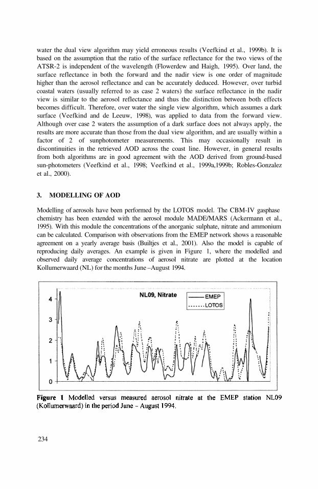
water the dual view algorithm may yield erroneous results (Veefkind et al., 1999b). It isbased on the assumption that the ratio of the surface reflectance for the two views of theATSR-2 is independent of the wavelength (Flowerdew and Haigh, 1995). Over land, thesurface reflectance in both the forward and the nadir view is one order of magnitudehigher than the aerosol reflectance and can be accurately deduced. However, over turbidcoastal waters (usually referred to as case 2 waters) the surface reflectance in the nadirview is similar to the aerosol reflectance and thus the distinction between both effectsbecomes difficult. Therefore, over water the single view algorithm, which assumes a darksurface (Veefkind and de Leeuw, 1998), was applied to data from the forward view.Although over case 2 waters the assumption of a dark surface does not always apply, theresults are more accurate than those from the dual view algorithm, and are usually within afactor of 2 of sunphotometer measurements. This may occasionally result indiscontinuities in the retrieved AOD across the coast line. However, in general resultsfrom both algorithms are in good agreement with the AOD derived from ground-basedsun-photometers (Veefkind et al., 1998; Veefkind et al., 1999a,1999b; Robles-Gonzalezet al., 2000).
Modelling of aerosols have been performed by the LOTOS model. The CBM-IV gasphasechemistry has been extended with the aerosol module MADE/MARS (Ackermann et al.,1995). With this module the concentrations of the anorganic sulphate, nitrate and ammoniumcan be calculated. Comparison with observations from the EMEP network shows a reasonableagreement on a yearly average basis (Builtjes et al., 2001). Also the model is capable ofreproducing daily averages. An example is given in Figure 1, where the modelled andobserved daily average concentrations of aerosol nitrate are plotted at the locationKollumerwaard (NL) for the months June –August 1994.
234
3. MODELLING OF AOD

From Figure 1 it is seen that the model resolves the temporal fluctuations of the nitrateconcentration quite reasonable. Before results of LOTOS can be compared and laterassimilated with the AOD-values from ATSR, a conversion of aerosol mass concentrationto aerosol optical depth has to be performed. This is done using the assumption of TenBrink et al. (1996) that the sulphate and nitrate aerosols are in the form of theirammonium salts. Hence, the modeled AOD values are based only on the simulatedconcentrations of sulphate and nitrate: primary aerosol as well as organic and sea saltaerosols are missing. On the one hand this is due to the fact that the latter two are notmodeled (yet) in LOTOS. On the other hand, the contribution of the primary aerosols tothe total AOD could not be computed because no information is available on theirextinction coefficients. Therefore we applied a factor of two to the modeled AOD in orderto correct for the ‘missing’ aerosols. This is in agreement with ground level observations,which indicate that anorganic aerosols contribute for about 50% to the total mass of
We realize that this is rather crude, but doing so results into observed and modeledAOD values that are in the same range and enables the application of data assimilation.The assumption is also made that all aerosols are contained in the lower part of thetroposphere (up to about 2 km). Recall that this study is only meant as a feasibility study,aimed at investigating the applicability of satellite retrieved aerosol information.
4. DATA ASSIMILATION OF AEROSOL SATELLITE DATA WITH LOTOS
Three data assimilation simulations for the month August 1997 have been carried out.Below the measurements that are used in the simulations are described, followed by aspecification of the simulations and a presentation and discussion of their results. Fordetails on the data assimilation technique used (a special version of the Kalman Filter), theinterested reader is referred to Builtjes at al. (2001).
4.1 Measurements taken into account
Apart from AOD fields also ground level ozone measurements have been assimilated intwo of the three simulations. The first reason to include ozone measurements is because alot of experience with assimilation of ozone measurements into LOTOS has been obtainedin a number of previous studies (see for example van Loon et al., 1999; van Loon et al.,2000). These studies showed the capability of the Kalman Filter technique to improveozone simulations by LOTOS. The second, more important, reason is that secondaryaerosol formation and ozone formation are coupled processes because both have in partthe same precursors. Also, a number of overlapping (non-emitted) chemical compoundsplays a role in both secondary aerosol formation and ozone production (for example
and the OH radical). Therefore, the assimilation of ozone measurements will have apotential impact on the secondary aerosol concentrations and vice versa. Hence it isinteresting to examine the behavior of the system when in addition to ozone measurementsalso AOD fields are assimilated.
AOD values from ATSR2 have been derived over Europe for August 1997 at the pixelsize of ATSR, The time of the overpass is at about 10:30 GMT, the frequency isonce per three days. The observed AOD fields have been aggregated to averages over the
235
LOTOS grid cells. The LOTOS grid cells are 0.5*1.0 latlong. The standard deviation (tobe used in the data assimilation) is set to 20% of the aggregated values. The number ofgrid cells for which an average could be determined varied from 255-700, with oneexception: on August 22 only 78 grid cells were covered. Recall that only cloud-freepixels can be taken into account. This explains why the number of grid cells for which anaverage can be constructed is varying.
The ozone observations consisted of a selected set of measurement from the EMEPnetwork (18) and the UBA network (9), as listed in Table 1.
In principle, also aerosol sulphate and nitrate observations could have been used in thedata assimilation procedure. However, the analysis has shown that the uncertainty in thenitrate observations is very large. Also, because of the fact that cloud chemistry is notincluded in LOTOS yet, a direct assimilation of sulphate observations and calculationsmight lead to dubious results. In forthcoming studies we hope to address this matter, asLOTOS is to be extended with cloud processes in the near future.
236
4.2 Description of the simulations
Three data assimilation simulations over the month August 1997 have been carried out.The measurements that have been assimilated in these simulations were:
Simulation 1: retrieved AOD fields + a set of ground level ozone measurementsfrom the EMEP and UBA networkSimulation 2: only the retrieved AOD fieldsSimulation 3: only the ozone ground level measurements.
As is described earlier, the modeled fraction of the AOD values is estimated to be 50% ofthe measured values. Hence the observed values have been divided by two to account forthe model fraction. In the remainder of this paper we will refer to a model simulationwithout data assimilation as ‘model’.In all three assimilation simulations the same noise specifications have been used. Colorednoise with a correlation length of 12 hours has been added to the emission fields of
and VOC. The standard deviations have been set to 50%. This may seem rather
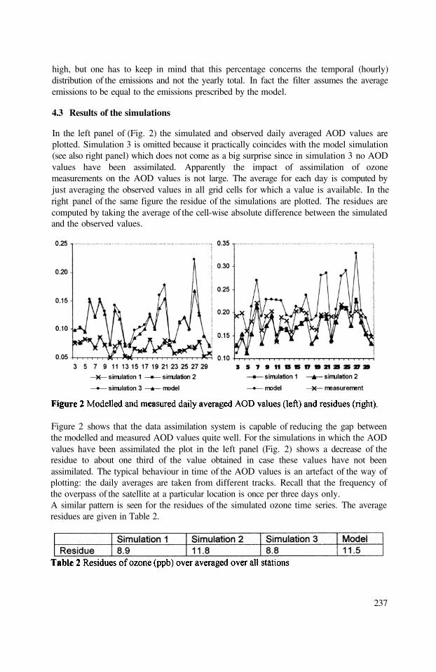
high, but one has to keep in mind that this percentage concerns the temporal (hourly)distribution of the emissions and not the yearly total. In fact the filter assumes the averageemissions to be equal to the emissions prescribed by the model.
4.3 Results of the simulations
In the left panel of (Fig. 2) the simulated and observed daily averaged AOD values areplotted. Simulation 3 is omitted because it practically coincides with the model simulation(see also right panel) which does not come as a big surprise since in simulation 3 no AODvalues have been assimilated. Apparently the impact of assimilation of ozonemeasurements on the AOD values is not large. The average for each day is computed byjust averaging the observed values in all grid cells for which a value is available. In theright panel of the same figure the residue of the simulations are plotted. The residues arecomputed by taking the average of the cell-wise absolute difference between the simulatedand the observed values.
Figure 2 shows that the data assimilation system is capable of reducing the gap betweenthe modelled and measured AOD values quite well. For the simulations in which the AODvalues have been assimilated the plot in the left panel (Fig. 2) shows a decrease of theresidue to about one third of the value obtained in case these values have not beenassimilated. The typical behaviour in time of the AOD values is an artefact of the way ofplotting: the daily averages are taken from different tracks. Recall that the frequency ofthe overpass of the satellite at a particular location is once per three days only.A similar pattern is seen for the residues of the simulated ozone time series. The averageresidues are given in Table 2.
237

Again we see that the residues from simulations in which ozone measurements areassimilated, are very close to each other. The same holds for the simulations in which theyhave not been assimilated.
The final product of the preceding chapter is the total hour-by-hour AOD-field over Europe ongrids of 0.5x1.0 lat-lon based on satellite observations and model results.The aim of the project is to derive air quality relevant information from the satellite data.There is a clear relation of AOD with fine particles, as The satellite sees in fact alarge part of theUsing data-assimilation, the original sulphate and nitrate AOD from LOTOS (already firstmultiplied with the described factor 2) have been corrected by the noise factors based onthe satellite AOD. These corrected sulphate+nitrate values in the mixing layer can be seenas the best estimate of concentrations which can be made using the satellite data asstarting point. In Figure 3 the averaged concentrations of for August 1997 aregiven that are determined in this way.
The assessment of the overall quality and accuracy of this result is difficult to give. Thisproject has led to a method by which can be determined from satellites in principle,however the current method contains many assumptions and weaknesses. They can be listed asfollows:
1. The current version of the LOTOS-model contains only sulphate and nitrate aerosol,
238
5. CONCLUSIONS AND OUTLOOK
which is only a part of the total The model should be extended to includeorganic aerosols and anthropogenic and natural primary emissions, and the chemicalcomposition of these to be able to determine extinction-coefficients. When theLOTOS-model is ‘ complete’, the current factor 2 can be abandoned. Although thismight not be so serious for the month of August 1997, the impact of cloud chemistrywill be more important for other months.The LOTOS model should be extended to incorporate cloud chemistry. Although thecurrent underestimation of sulphate and nitrate will be compensated by applyingdata-assimilation, the resulting noise factors for emissions are unrealistic because theunderestimation is due to the missing cloud chemistryThe assumption is that all aerosols contributing to the AOD-values are in the lower,say 3 km, of the atmosphere. When this is not the case, the current method will leadto an overestimation ofThe current method uses only the AOD-values from ATSR-2 for inclusion in thedata-assimilation procedure. Although very valuable, the amount of observations isrelatively scarce, a maximum of 11 observations per month per pixel, which meanson a total of 744 hours per month only in about 1.5 % of the cases (in fact thesatellite observation is not an hourly averaged value, but much shorter). The use of ageo-stationary satellite would be a great improvement in this respect. In the data-assimilation also ground-level observations of sulphate could be included to improvethe output of the system. The same holds for other observations, like nitrate, or
if they are of good quality.The Angstrom coefficient which is also determined from ATSR gives an indicationof the size distribution of the aerosols. This information could be used, incombination with the LOTOS-model, to improve the accuracy of the currentestimatesCalculations can be performed on fine scales by using UAM+aerosols (a nestedversion of LOTOS with grid sizes that can be as fine as These resultscould also be assimilated with the fine-scale AOD-values from ATSR to obtaindetailed information for selected areas, for example a specific city. This mightimprove the current concentrations, and could help to determine whether thefound large spatial gradients in observed AOD-values are a result of local primaryemissions of
239
In principle, all the above given 6 points can be improved upon.
The method described here is in principle working, taking all the uncertainties which could beimproved upon, for granted. It should be noted that at the moment the retrieval of AOD israther time consuming because there is no operational and automated method yet to determinewhether a pixel is cloud free or not.The method would gain in accuracy in case reliable ground level observations would beavailable. Lidar observations are useful to determine whether indeed all aerosols are below 3km, but they seem not to be strictly needed for an operational method.In conclusion, a method has been developed by which concentrations can be determinedat fine spatial scales, down to in principle 1x1 km2, using satellite observations. The currentmethod might have an accuracy of only a factor 2-3. Most of the current weaknesses of the
2.
3.
4.
5.
6.
method can be improved upon, as is indicated in the 6 points mentioned.So, in conclusion, using satellite data in combination with a validated model with dataassimilation, a method has been developed by which estimates of at ground level can bedetermined.The recommendation is that, referring to the points mentioned above, the method should beimproved and applied to a finer grid scale. Also, a more automated method should bedeveloped for the determination of a pixel being could-free or not.
The project was funded by the Netherlands Remote Sensing Board (BCRS) and by theTNO internal project ‘Dedicated Aerosol Retrievals using Earth Observation (DARE)’.
Ackermann I. J., H. Hass, M. Memmesheimer, C. Ziegenbein, A. Ebel, 1995, Theparametrization of the sulphate-nitrate-ammonia aerosol system in the long rangetransport model EURAD, Meteorol. Atmos. Phys., 57: 101.
Brink, H.M. ten, J. P. Veefkind, A. Waijers-IJpelaan, and J. C. van der Hage, 1996,Aerosol light-scattering in The Netherlands, Atmospheric Environment, 30:251.
Builtjes, P.J.H. et al., 2001 (in press), Aerosol Air Quality Satellite Data, Final Report ofBCRS project 4.1/AP-06.
Flowerdew R. J., and J. D. Haigh, 1995, An approximation to improve accuracy in thederivation of surface reflectances from multi-look satellite radiometers, Geophysicalresearch letters, 23: 1693.
Loon, M. van, P.J.H. Builtjes, and M.G.M. Roemer, 1999, Reactive trace gas dataassimilation – Final Report. BCRS publication USP-2 99-12.
Loon, M. van, I. J. Ackermann, M. Schaap, and P. J. H. Builtjes, 2000, Primary andsecondary aerosol simulation using LOTOS, J. Aerosol Sci., 31(Suppl. 1): S52.
Robles Gonzalez C., J. P. Veefkind, and G. de Leeuw, 2000, Aerosol optical depth overEurope in August 1997 derived from ATSR-2 data, Geophysical Research Letters,27 (No 7):955.
Veefkind J. P., G. de Leeuw, P. A. Durkee, 1998, Retrieval of Aerosol Optical Depthover Land using two angle view Satellite Radiometry during TARFOX, GeophysicalResearch Letters, 25: 3135.
Veefkind J. P., G. de Leeuw, P. A. Durkee, P. B. Russell, P. V. Hobbs, and J. M.Livingston, 1999a, Aerosol optical depth retrieval using ATSR-2 data and AVHRRdata during TARFOX, J. Geophys. Res., 104 (D2):2253.
Veefkind J. P., G. de Leeuw, P. Stammes, R. B. A. Koelemeijer, 1999b, RegionalDistribution of Aerosol over land derived from ATSR-2 and GOME, Accepted forpublication in Rem. Sens. of the Env.
240
6. ACKNOWLEDGEMENT
7. REFERENCES

DISCUSSION
What is the reason for the large discrepancies you observedbetween modelling results and measurements ?
M. VAN LOON The particular station shown in the presentation (Vredepeel, NL,EMEP station NL10) is known to be a difficult one. In general theagreement of LOTOS results with measurements is much better.At the same time, it was shown that with small adaptations (onaverage) to the model input the (assimilated) concentrations asproduced by LOTOS are in much better agreement with themeasurements.
A. HANSEN Have you considered varying other parameters than emissionsplus PM and deposition as part of your assimilation andoptimization scheme ?
M. VAN LOON Yes. But we have not done this yet, because of the increasingcomputational burden. In principle, all uncertainties that arepresent in the model and are likely to have impacts on thequantities to be assimilated, should be taken into account. Thepresent study therefore only shows that non-linear dataassimilation of ozone and aerosols can be a powerful tool. Thevalues of the “noise” factors should not be taken for “real”estimates of emissions and deposition velocities.
Following the previous question concerning discrepanciesbetween model and observation, which type of cloud chemistrydescription is used in the model ?
M. VAN LOON A simple parameterisation considering mainly sulphate andammonium chemistry, i.e. oxidation of to aerosols by
and/or ozone and conversion into aerosols.
A. EBEL Is an improvement of simulated concentrations through theassimilation of observed ozone data also noticed for otherchemical species, e.g. (or which have not beenassimilated ?
241
S. VARDOULAKIS
N. FOURNIER

M. VAN LOON In principle this should be the case. However, the model used(LOTOS) is not suited for modelling of primary species (e.g.
VOC) and is known to underestimate by a factor of 2 to3. This is due to the mixing layer concept used in LOTOS.
242
SIMULATING SOIL-DUST, SEA-SALT AND SULFATEAEROSOLS IN EAST ASIA USING RAMS-ONLINE
CHEMICAL TRANSPORT MODEL COUPLED WITHCAM (CANADIAN AEROSOL MODULE)
Zifa Wang, Itsushi Uno, Sunling Gong, Meigen Zhang, and Hajime Akimoto*
1. INTRODUCTION
Aerosols are currently the focus of many studies due to the large uncertainties intheir indirect radiative forcing, particle pollution, and to the adverse health effectsassociated with them (Penner, 1993). Aerosol processes in the East Asia region are ofparticular interest because anthropogenic emissions in this region are increasing rapidlyand supplement the natural production of mineral dust, which together play an importantrole in tropospheric chemistry and regional and global climate change. The particles inthe continental flow over East Asia consist of a complex, partially externally mixedcombination of sea-salt aerosol, combustion-derived particles, including organic and sootcomponents, mineral dust, and biogenic non-sea-salt sulfate and organic particles (Songand Carmichael, 2001; Uno et al., 2001a;b; Wang et al., 1996; 2000). The outflow ofAsian aerosols may affect the chemistry and radiation budgets over a large area of theNorth Pacific(Qian, et al., 2001). However, tropospheric aerosols are poorlycharacterized in global and regional climate models, and thus introduce a substantialuncertainty into predictions of climate change.
To improve this situation, both intensive measurements and comprehensive physicaland chemical modeling on global and regional scales are required. Since the radiativeproperties of an aerosol population depend on the chemical composition, size distribution,and mixing state, models that resolve these characteristics are required. In this paper, weapply an online chemistry transport model system (OCTMs) coupled with RAMS(Regional Atmospheric Modeling System) to study the evolution of aerosol particles andtheir physical and chemical properties in the Asian Pacific region. The model system,
Zifa Wang, Itsushi Uno, Meigen Zhang, Hajime Akimoto, Frontier Research System for Global Change,IGCR-Yokohama, 3173-25 Showa-machi, Yokohama 236-0001, Japan. Sunling Gong, AtmosphericEnvironment Service, 4905 Dufferin Street, Downsview, Ontario M3H 5T4 Canada.
Air Pollution Modeling and Its Application XV, Edited byBorrego and Schayes, Kluwer Academic/Plenum Publishers, New York, 2002 243
*

which has also been coupled with the Canadian Aerosol Module (CAM), is capable ofresolving the size and composition of aerosols of multiple types and providing theregional distribution of size-segregated sulfate, black carbon, soil dust, and sea-saltaerosols over the East Asia. Simulated total aerosol concentrations were evaluated withobservations from an aircraft campaign along the coast of China in May 1993. Details ofthe regional soil dust, sea-salt and sulfur distribution are also addressed from thesimulation as a function of particle size.
2. MODEL DESCRIPTION
An on-line chemical transport model system has been developed and applied tosimulate the trans-Pacific transport of yellow sand and sulfur (Uno et al. 2001a, 2001b).In the system, the parallel version (4.3) of RAMS is used to simulate the meteorologicalfields including boundary turbulence, clouds and precipitation. A general description ofRAMS and its capabilities are given by Pielke et al. (1992). RAMS includes the Kuo-type cumulus parameterization to represent sub-grid convective cumulus and a Kessler-type microphysical model (Walko et al., 1995). The surface flux calculation module inRAMS was improved on the basis of the results of Uno et al. (1995).
A tracer transport model and the Canadian Aerosol Module (CAM) are fully coupledwith RAMS with various options for representing the physical and chemical processesdescribing regional- and urban-scale atmospheric pollution. This is a unique approach toprovide on-line the regional meteorological conditions, such as precipitation, cloudmicrophysics, the turbulence in the boundary layer, and vertical diffusion, which play asignificant role in the evolution of the tracers. The on-line tracer model runs with thesame time step as RAMS, so all the meteorological information is directly used by thetracer transport model at every time step.
The gas-phase chemical reaction scheme used in the present work is a slightlymodified version of the CBM-IV (Gery et al., 1989). Values of the reaction ratecoefficient are updated with recent kinetic data and a more detailed chemistry of SOx isincorporated (Wang et al., 1996). The modified mechanism includes 34 species and 86photochemical, inorganic and organic reactions. The removal term is usually separatedinto dry removal due to sedimentation and deposition at the surface and wet removal dueto precipitation.
CAM is a size-segregated multi-component aerosol algorithm which includes majoraerosol processes in the atmosphere: production, growth, coagulation, nucleation,condensation, dry deposition, below-cloud scavenging, and activation, and includes anexplicit micro-physical cloud module to treat the aerosol-cloud interactions and chemicaltransformation of sulfur species in clear air and in clouds [Gong et al., 2001]. In CAM,the mass conservation equations are written for dry aerosol mass mixing ratio while theremoval rates such as dry deposition and coagulation are calculated based on wet aerosolsize. At the beginning of each time step, the ambient radius of aerosols in each bin iscomputed according to the relative humidity and composition. Nine bins are selected forthe simulation with mid-radius of 0.03, 0.06, 0.12, 0.24, 0.48, 0.96, 1.92, 3.84, and
244
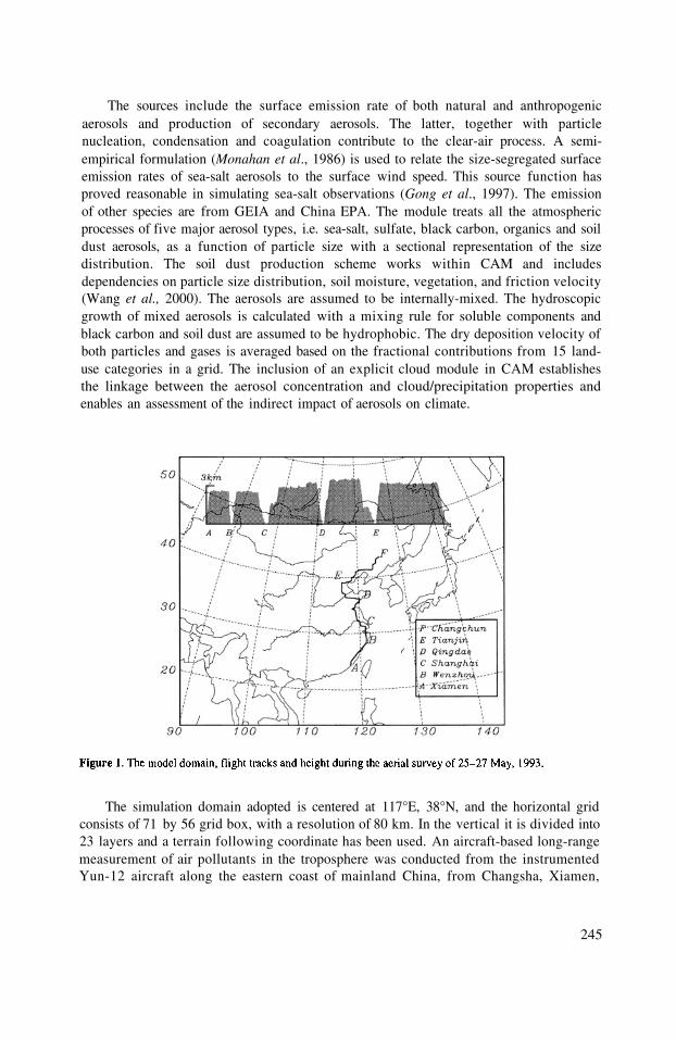
The sources include the surface emission rate of both natural and anthropogenicaerosols and production of secondary aerosols. The latter, together with particlenucleation, condensation and coagulation contribute to the clear-air process. A semi-empirical formulation (Monahan et al., 1986) is used to relate the size-segregated surfaceemission rates of sea-salt aerosols to the surface wind speed. This source function hasproved reasonable in simulating sea-salt observations (Gong et al., 1997). The emissionof other species are from GEIA and China EPA. The module treats all the atmosphericprocesses of five major aerosol types, i.e. sea-salt, sulfate, black carbon, organics and soildust aerosols, as a function of particle size with a sectional representation of the sizedistribution. The soil dust production scheme works within CAM and includesdependencies on particle size distribution, soil moisture, vegetation, and friction velocity(Wang et al., 2000). The aerosols are assumed to be internally-mixed. The hydroscopicgrowth of mixed aerosols is calculated with a mixing rule for soluble components andblack carbon and soil dust are assumed to be hydrophobic. The dry deposition velocity ofboth particles and gases is averaged based on the fractional contributions from 15 land-use categories in a grid. The inclusion of an explicit cloud module in CAM establishesthe linkage between the aerosol concentration and cloud/precipitation properties andenables an assessment of the indirect impact of aerosols on climate.
The simulation domain adopted is centered at 117°E, 38°N, and the horizontal gridconsists of 71 by 56 grid box, with a resolution of 80 km. In the vertical it is divided into23 layers and a terrain following coordinate has been used. An aircraft-based long-rangemeasurement of air pollutants in the troposphere was conducted from the instrumentedYun-12 aircraft along the eastern coast of mainland China, from Changsha, Xiamen,
245
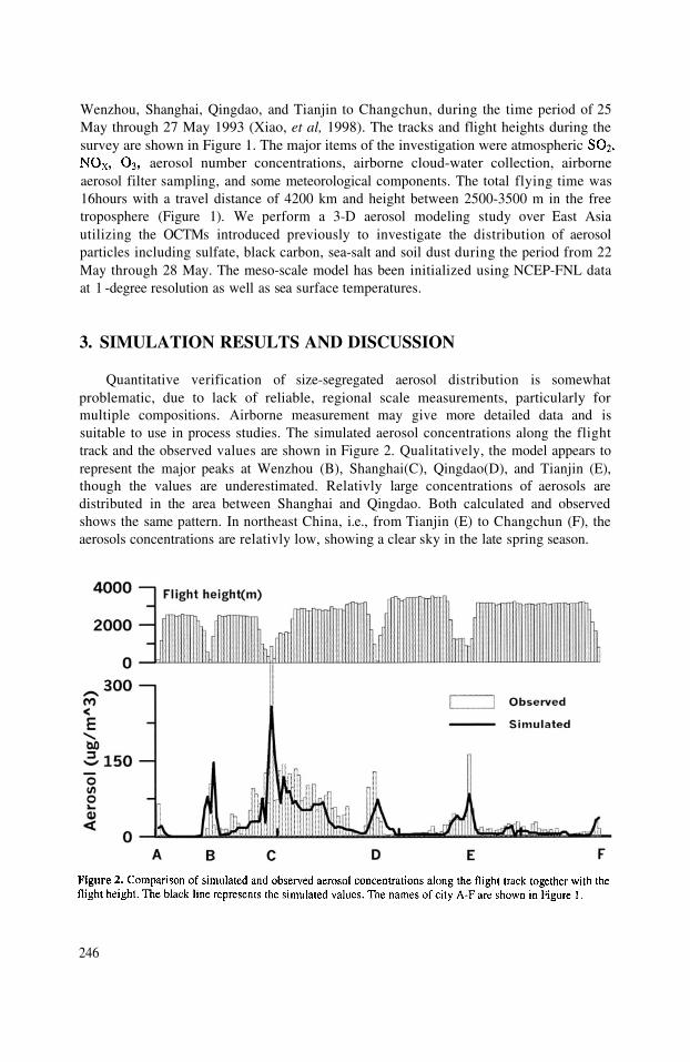
Wenzhou, Shanghai, Qingdao, and Tianjin to Changchun, during the time period of 25May through 27 May 1993 (Xiao, et al, 1998). The tracks and flight heights during thesurvey are shown in Figure 1. The major items of the investigation were atmospheric
aerosol number concentrations, airborne cloud-water collection, airborneaerosol filter sampling, and some meteorological components. The total flying time was16hours with a travel distance of 4200 km and height between 2500-3500 m in the freetroposphere (Figure 1). We perform a 3-D aerosol modeling study over East Asiautilizing the OCTMs introduced previously to investigate the distribution of aerosolparticles including sulfate, black carbon, sea-salt and soil dust during the period from 22May through 28 May. The meso-scale model has been initialized using NCEP-FNL dataat 1 -degree resolution as well as sea surface temperatures.
3. SIMULATION RESULTS AND DISCUSSION
Quantitative verification of size-segregated aerosol distribution is somewhatproblematic, due to lack of reliable, regional scale measurements, particularly formultiple compositions. Airborne measurement may give more detailed data and issuitable to use in process studies. The simulated aerosol concentrations along the flighttrack and the observed values are shown in Figure 2. Qualitatively, the model appears torepresent the major peaks at Wenzhou (B), Shanghai(C), Qingdao(D), and Tianjin (E),though the values are underestimated. Relativly large concentrations of aerosols aredistributed in the area between Shanghai and Qingdao. Both calculated and observedshows the same pattern. In northeast China, i.e., from Tianjin (E) to Changchun (F), theaerosols concentrations are relativly low, showing a clear sky in the late spring season.
246

The evolution and fate of atmospheric aerosols are influenced by various dynamicaerosol processes, which cannot be constrained by measurements alone. Figure 3 showsthe simulated and observed size distribution of aerosol particles over Shanghai at 100meters above the surface. The two peaks are simulated well compared with theobservations; one peak is mainly composed of sulfate and black carbon, and the other ismainly from sea-salt particles. The simulation results show that when the size is less than
the main components of the particles are black carbon and sulfate, and for sizeslarger than nearly all the particles are sea-salt over Shanghai.
The distribution of sulfate, sea-salt, black carbon and soil dust particles in theboundary layer on May 22 are presented in Figure 4. The sulfate distribution showsclearly the high concentration regions in East China including Shanghai and the Qingdaoarea. The observations also show a similar pattern along the flight tracks. The sea-saltparticles are mainly distributed in the Japan Sea and the area east towards Taiwan. Thereis also a small area with high sea-salt concentrations near Shanghai, which accounts for
247
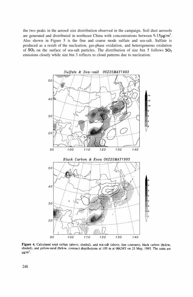
the two peaks in the aerosol size distribution observed in the campaign. Soil dust aerosolsare generated and distributed in northeast China with concentrations betweenAlso shown in Figure 5 is the fine and coarse mode sulfate and sea-salt. Sulfate isproduced as a result of the nucleation, gas-phase oxidation, and heterogeneous oxidationof on the surface of sea-salt particles. The distribution of size bin 5 followsemissions closely while size bin 3 reflects to cloud patterns due to nucleation.
248
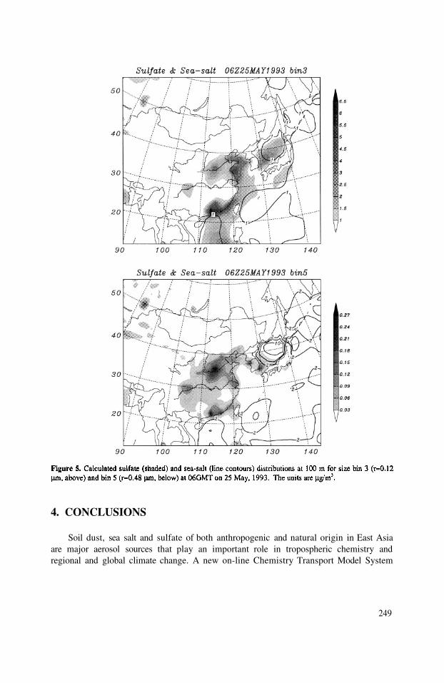
4. CONCLUSIONS
Soil dust, sea salt and sulfate of both anthropogenic and natural origin in East Asiaare major aerosol sources that play an important role in tropospheric chemistry andregional and global climate change. A new on-line Chemistry Transport Model System
249

(OCTMs) is developed to simulate the regional distribution of size-segregated soil-dust,sea-salt, black carbon and sulfate aerosols in the atmosphere in East Asia. It considersadvection, diffusion, chemistry, and deposition processes and is fully coupled with theCanadian Aerosol Module (CAM) and CSU-RAMS (Regional Atmospheric ModelingSystem. The CAM is a size-segregated multi-component aerosol algorithm whichincludes major aerosol processes such as production, coagulation, nucleation,condensation, dry deposition, below-cloud scavenging, and activation, and includes anexplicit micro-physical cloud module to treat the aerosol-cloud interactions and chemicaltransformations. The soil dust production scheme works within the CAM and includesdependencies on particle size distribution, soil moisture, vegetation, and friction velocity.Simulated aerosol concentrations are evaluated against observations from an aircraftcampaign along the coast of China in May 1993 and reasonable agreement is reached.
REFERENCES
Gery, M. W., Whitten, G.Z., Killus, J.P., and Dodge, M.C. 1989, A photochemical kinetics mechanism forurban and regional scale computer modeling. J. Geophys. Res. 94: 12,925-12,956.
Gong, S.L., L.A., Barrie, and J.-P., Blanchet, 1997, Modeling sea-salt aerosols in the atmosphere, Part 1: Modeldevelopment, J. Geophys. Res., 102: 3805-3818.
Gong, S.L., L.A., Barrie, et. al, 2001, CAM: Treatment of the size segregated atmospheric aerosols for climateand air quality models: 1. Module Development, J. Geophys. Res.(submitted).
Monahan, E.C., D.E., Spiel, and K.L., Davidson, 1986, A model of marine aerosol generation via whitecaps andwave disruption, in Oceanic Whitecaps, Monnhan, D., and G.M. Niocaill, ed., Redeil Publishing,Dordrecht, Holland, pp. 167-174.
Penner, J., 1993, Quantifying and minimizing uncertainty of climate forcing by anthropogenic aerosols,technical report, U.S. Dep. of Energy, Washington, D.C., pp.53.
Pielke, R.A., W.R. Cotton, R.L. Walko, C.J. Tremback, W.A. Lyons, L.D. Grasso, M.E. Nicholls, M.D. Moran,D.A. Wesly, T.J. Lee, and J.H. Copeland, 1992, A comprehensive meteorological modeling system-RAMS, Meteorol. Almos. Phys., 49:69-91.
Qian, Y., F. Giorgi, Y. Huang, W. Chameides and C. Luo, Regional simulation of anthropogenic sulfur overEast Asia and its sensitivity to model parameters, Tellus, 53B:171-191.
Song, C.-H., and G.R., Carmichael, 2001, A three-dimensional modeling investigation of the evolutionprocesses of dust and sea-salt particles in east Asia, J. Geophy. Res., 106: 18,131-18,154.
Uno, I., S. Emori, and M. Baldi, 2001a, Chemical transport model on-line coupled with RAMS for regionalchemical climate, in Air Pollution Modeling and its Application XIV, Grying and Schiermeier, Ed.,Kluwer Academic/Plenum Publishers, New York, pp.75-85.
Uno, I., H., Amano, S., Emori, K., Kinoshita, I., Matsui, and N., Sugimoto, 2001b, Trans-Pacific yellow sandtransport observed in April 1998: A numerical simulation, J. Geophy. Res., 106:18,331-18,344.
Walko, R.L., W.R. Cotton, M.P. Meyers, and J.Y. Harrington, 1995, New RAMS cloud microphysicsparameterization, Part I, The single-moment scheme, Atmos. Res., 38:29-62.
Wang, Z., Huang, M., He, D., Xu, H., and Zhou, L., 1996, Sulfur distribution and transport studies in East Asiausing Eulerian model, Advances in Atmospheric Sciences 13:399-409.
Wang, Z., H. Ueda and M. Huang, 2000, A deflation module for use in modeling long-range transport of yellowsand over East Asia, J. Geophy. Res., 105:26,947 -26,960.
Xiao, H., Y. Wu, Z. Shen, Z. Wang, H. Lei, and L. Zhou, 1998, Aircraft-based measurements of atmosphericpollutants in the troposphere over the eastern coast of China, in Air Quality and Atmospheric Science,Proceedings of the 6thinternational conference on atmospheric science and its applications to air quality,Chen, Ed., China Ocean Press, pp. 398-406.
250

DISCUSSION
P. SUPPAN
Z. WANG
A. HANSEN
Z. WANG
E. GENIKHOVICH
Z. WANG
How many size segments have you used ?
Nine bins are used in the model, they are of mid-radius 0.03, 0.06,0.12, 0.48, 0.96, 1.92, 3.84 and
It appears that your model may be over-estimating nucleation inthe nano-particle size range. It seems to me that in these areas ofhigh particle loadings, you would not expect nucleation, but rathercondensation on existing particles. Do you agree ?
Thank you for your comments. Comparing with observations, itappears the model over-estimated nucleation in the particle sizerange. We need better quality observation data to evaluate themodel results, especially for the size distribution and detailedchecking of the micro-physical process in the CAM.
What were temporal and spatial averaging scales for measuredand computed quantities ? How did you handle the fact thatmeasurements were carried out from the moving platform andcomputations were not ?
This is a good question. The temporal and spatial resolutions ofmeasured data is about 5-minute and about 70 km. For the modelcomputation, the temporal resolution is the same as in theobservations, but for the spatial resolution (80 km), someinterpolation errors can occur. We need to improve this as thefuture by using a higher resolution model or nested model.
251

This page intentionally left blank

NEW DEVELOPMENTS
Chairpersons :
Rapporteurs :
E. BatchvarovaC. BorregoS.E. GryningR. San Jose
K. De RidderJ. FerreiraC. HogrefeA. Keiko

This page intentionally left blank

DATA ASSIMILATION FOR CT-MODELLING BASEDON OPTIMUM INTERPOLATION
Johannes Flemming, Eberhard Reimer, and Rainer Stern*
1 INTRODUCTION
Several studies to apply data assimilation to Chemical Transport Models (CTM)have been carried out in recent years (e.g. Elbern 1997, Loon 1997). There arecomprehensive time dependent schemes such as 4D-VAR or Kalman-Bucy-Filters ormore simpler 3/2D-schemes such as Optimum Interpolation and 3D-VAR. Providinginitial fields for numerical weather forecasting which obey the physical laws andbalance relationships has been the main motive for the development of dataassimilation. The use of the techniques from numerical weather forecasting in chemistrytransport modelling requires the adaptation to the special properties of the chemicalconcentration measurements and the CTMs.
The content of this paper is data assimilation for the Eulerian chemical transportmodel REM3 by means of Optimum Interpolation (OI). The focus is put on theimplementation of OI for the inhomogeneous air quality data in section 4. Dataassimilation with REM3 has been used for the diagnostic assessment of air qualitystandards according to the air quality framework directive (96/62/EC) of the EuropeanCouncil. An example of this work (NO2 concentrations in Germany) will be presentedin section 5. Moreover, OI is employed for initialising the operational ozone forecastscarried out at the FU-Berlin.
The main result of data assimilation for Eulerian type models is an analysis of theconcentrations field. The analysis is a representation of the concentration field in acertain resolution which is determined by the underlying model. It combines the fieldsof the model with observations. Both sources of information are blended according totheir error statistics. This is a feature of all statistical based data assimilation techniques.
Optimum Interpolation (Gandin 1962) is an interpolation technique and can becompared to other spatial interpolation methods either based on statistics such asKriging or on “purely mathematical” methods such as spline interpolation and distancedensity interpolation (Egmond Van 1981). The differences of the methods concern three
* Institut für Meteorologie, Freie Universität Berlin, 12165 Berlin, Germany
Air Pollution Modeling and Its Application XV, Edited byBorrego and Schayes, Kluwer Academic/Plenum Publishers, New York, 2002 255

points: 1.) How are the measurement values weighted to form the value at analysispoint. 2.) Whether and how the observation error is taken into account. 3.) Whether theimpact of an inhomogeneous measurement network (declustering, Falke 1998) iscompensated. A brief discussion of the properties and the equations of OptimumInterpolation is the content of section 3.
The performance of Optimum Interpolation depends on the efforts to determineerror statistics. The proper determination of the error statistics, .i.e. the observation errorvariance and the background error covariance matrix, is essential for the success of theanalysis scheme.
However, the application of those methods for ground based measurement of airquality data is not straight forward. One has to consider the inhomogeneous character ofthe concentration field due to the inhomogeneous emission patterns and the more densenet work in the urban environment. Section 4.2 deals with the determination of the errorstatistics for concentration data which discriminates different air pollution regimes inthe measurements and in the calculated fields.
2 DESCRIPTION OF THE MODEL AND THE AIR QUALITY DATA BASE
REM3 (Stern 1994) is a transport model for the Planetary boundary layer thatcovers the area of Central Europe with a horizontal resolution of about 25x25 km. Thevertical resolution of the model is based on three dynamically changing layers. CBM4and SAPRC are the alternative chemistry schemes used in the model. Recently REM3has been merged with the model CALGRID to form REM3/CALGRID - a model whichoffers a flexible way to treat different horizontal and vertical coordinate systems andincludes aerosol modeling. Meteorological input is derived from synoptic meteorolo-gical surface data, upper air data and climatological information (Reimer and Scherer1992). REM3 has been employed successfully for episodic applications (Hass 1997)and emission scenario calculations (http://www.umweltbundesamt.de/ozon-e). Currentapplications include the calculation of air quality standards for O3, NO2, SO2 andPM10 on a yearly basis according to the European Council Directive 96/62/EC. REM3also runs operationally to forecast the ozone concentration in Central Europe since 1997(Flemming 2001, http://trumf.fu-berlin.de/ozonprognose/).
The air quality data base has been obtained from the networks of the German states(Laender). It includes about 250 measurement sites for O3, NO2 and NO. Lessmeasurement (about 150) are available for SO2 and TSP (total suspended matter).Additionally, measurements from other European countries have been acquired from theEMEP and the EEA data base. The data quality assurance (EU-directive) demands 90%completeness for the yearly time series. To meet this requirement about 15% (Ozone) to50% (NO) of the data had to be rejected.
By means of a hierarchical clustering the measurement sites were classified in airquality regimes (Flemming 2001). The parameters for distinguishing the regimes are themedian of the daily mean and the median of the daily variability of the time series forthe years 1995-99. For each species separately regimes such as “mountain”, “rural”,“suburban”, “urban”, “urban-traffic” and “traffic” were identified.
The air quality regimes are a comprehensive climatological measure. It is fruitful toapply this concept also to modelled concentration time series. The centres of the clustersfrom the observed data in the parameter space were used to assign an air quality regimeto every grid point of the REM3/CALGRID modelling area. The parameters for everymodel grid point were determined from a model run for the whole year 1999.
256
3 OPTIMUM INTERPOLATION
Optimum Interpolation (OI) was introduced in meteorology by Gandin (1962). Itproduces an analysis by correcting a first guess field that is called background. Thebackground can be a calculated field, as in this application, a field derived from clima-tology or simply the mean of the measurements. An example of the application of OI forSO2 with the measured mean as background can be found in Egmond (1981).
In OI the value of the analysis xIa at grid point I is the sum of the background valuexIb and the weighted mean of measurements increments from N nearby measurementsites (Eq. 1). The measurement increments at the measurement locations i=1...N are thedifferences between the measured value yi and the respective background value xib.
The vector of analysis weights a are found from minimising the variance of theanalysis error with the additional constraint that the measurements and the backgroundfield have no mutual bias. This yields the following matrix equation:
B is the N x N covariance matrix of the background error at the measurementlocations. R is a diagonal matrix containing the error variances for each observation inthe diagonal line and zero elsewhere with the assumption that the observation error isnot mutually correlated. b is a vector of the N covariance values of the background errorbetween the measurement location and the analysis point I. Equation 2 leads to thefollowing features of OI:
The analysis weights ai are mainly determined by the covariances (vector b) ofthe background error between the measurement sites and the interpolationpoint.A low error variance of an observation enhances its influences in the analysis(diagonal elements of matrix R).High covariances between the background errors at two measurements sites(off diagonal elements of B) reduces the individual weight of theseobservations.
The observation error includes the instrument error and errors due the fact that ameasurement is not representative for the respective grid point value of the background(model field). The variance of the model error is a measure for the accuracy of modelfield at a certain point.
The covariance of the background describes the spatial relationship of the modelerror. Therefore it controls how far the influence of the measurement can be spread inthe spatial domain.
257
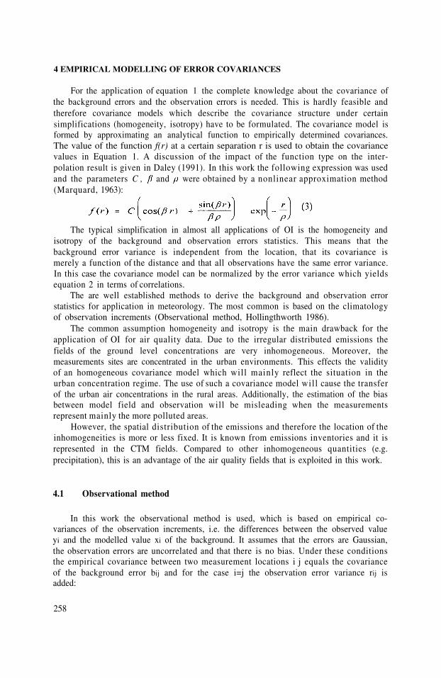
4 EMPIRICAL MODELLING OF ERROR COVARIANCES
For the application of equation 1 the complete knowledge about the covariance ofthe background errors and the observation errors is needed. This is hardly feasible andtherefore covariance models which describe the covariance structure under certainsimplifications (homogeneity, isotropy) have to be formulated. The covariance model isformed by approximating an analytical function to empirically determined covariances.The value of the function f(r) at a certain separation r is used to obtain the covariancevalues in Equation 1. A discussion of the impact of the function type on the inter-polation result is given in Daley (1991). In this work the following expression was usedand the parameters C , and were obtained by a nonlinear approximation method(Marquard, 1963):
The typical simplification in almost all applications of OI is the homogeneity andisotropy of the background and observation errors statistics. This means that thebackground error variance is independent from the location, that its covariance ismerely a function of the distance and that all observations have the same error variance.In this case the covariance model can be normalized by the error variance which yieldsequation 2 in terms of correlations.
The are well established methods to derive the background and observation errorstatistics for application in meteorology. The most common is based on the climatologyof observation increments (Observational method, Hollingthworth 1986).
The common assumption homogeneity and isotropy is the main drawback for theapplication of OI for air quality data. Due to the irregular distributed emissions thefields of the ground level concentrations are very inhomogeneous. Moreover, themeasurements sites are concentrated in the urban environments. This effects the validityof an homogeneous covariance model which will mainly reflect the situation in theurban concentration regime. The use of such a covariance model will cause the transferof the urban air concentrations in the rural areas. Additionally, the estimation of the biasbetween model field and observation will be misleading when the measurementsrepresent mainly the more polluted areas.
However, the spatial distribution of the emissions and therefore the location of theinhomogeneities is more or less fixed. It is known from emissions inventories and it isrepresented in the CTM fields. Compared to other inhomogeneous quantities (e.g.precipitation), this is an advantage of the air quality fields that is exploited in this work.
4.1 Observational method
In this work the observational method is used, which is based on empirical co-variances of the observation increments, i.e. the differences between the observed valueyi and the modelled value xi of the background. It assumes that the errors are Gaussian,the observation errors are uncorrelated and that there is no bias. Under these conditionsthe empirical covariance between two measurement locations i j equals the covarianceof the background error bij and for the case i=j the observation error variance rij isadded:
258

The value of the observation error can be estimated by extrapolating a covariancemodel to zero separation which yields bii. The difference to the variance of the in-crements equals the variance of the observation error rii.
The ensemble to calculate the empirical expectation value (Eq. 4) has to be chosenaccording to the minimising condition of equation 1 (Egmond Van 1981). Twoapproaches have been used for the OI of air quality data. One relies on the instant set ofmeasurements and the other is based on time series of the observation increments
A comparison of the different approaches for NO2 is given in section 5.Under homogeneous and isotropic conditions a covariance model can be fitted
by the data available at the time considered. The increments of the measurements withina an interval of separation are used to calculate the empirical spatial covariance directly.The covariance model is obtained from these covariance coefficients. The advantage ofthis approach is that no previous data are needed. The covariance model which iscalculated for each analysis date reflects the change in the mean spatial variability dueto temporal variations in the weather situations and the emissions. However, spatialpatterns (inhomogeneity) can not be distinguished.
The use of time series to calculate a empirical covariance of the backgrounderror is a common approach (Daley 1992). It leads to a large number of covariances foreach pair of stations which are the base for the approximation of the spatial covariancemodel (Eq. 3). This type of covariance reflects more the climatological situation. Thesize of the ensemble allows the discrimination of different classes of covariance models(see section 4.2.)
However, the temporal covariance may lead to an overestimation of the spatialcovariance due to temporal variations as the annual and diurnal cycle which have noequivalent in the spatial domain. If the increments show these variations they have to beremoved by filtering.
4.2 Inhomogeneous covariance models for air quality data
The base for the development of an inhomogeneous covariance structure is theclassification of the air quality regimes for both the measurements and the grid points ofthe model field which serves as the background for OI (see section 2). The knowledgeof the air quality regime of the whole background (i.e. the modelled field) is an im-provement for the interpolation performance because the covariance of the backgrounderror (B and b in Eq. 1) controls to a large extend the analysis weights. The observationerror is mainly an error of representativity. In this context it quantifies how good theregime of the measurement coincides with that of corresponding background point.
The objective was to build a set of covariance models, one for each possiblecombination of air quality regimes in the background field. The covariance model for agiven combination of regimes are supposed to have a simple distance dependency as inthe homogeneous and isotropic case. The inhomogeneous character of the OI comesfrom the selection of the covariance model according to the combination of the regimesat the points I and i or i and j. For this reason, it reflects the inhomogeneous distributionof the air quality as it was derived from the model results.
The observational method based on times series covariances (approach is appliedto obtain the covariance models. In order to avoid the influence of the diurnal cycle, the
259
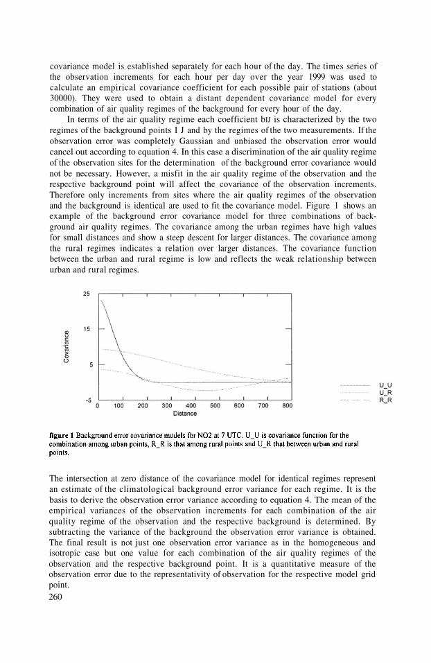
covariance model is established separately for each hour of the day. The times series ofthe observation increments for each hour per day over the year 1999 was used tocalculate an empirical covariance coefficient for each possible pair of stations (about30000). They were used to obtain a distant dependent covariance model for everycombination of air quality regimes of the background for every hour of the day.
In terms of the air quality regime each coefficient bIJ is characterized by the tworegimes of the background points I J and by the regimes of the two measurements. If theobservation error was completely Gaussian and unbiased the observation error wouldcancel out according to equation 4. In this case a discrimination of the air quality regimeof the observation sites for the determination of the background error covariance wouldnot be necessary. However, a misfit in the air quality regime of the observation and therespective background point will affect the covariance of the observation increments.Therefore only increments from sites where the air quality regimes of the observationand the background is identical are used to fit the covariance model. Figure 1 shows anexample of the background error covariance model for three combinations of back-ground air quality regimes. The covariance among the urban regimes have high valuesfor small distances and show a steep descent for larger distances. The covariance amongthe rural regimes indicates a relation over larger distances. The covariance functionbetween the urban and rural regime is low and reflects the weak relationship betweenurban and rural regimes.
The intersection at zero distance of the covariance model for identical regimes representan estimate of the climatological background error variance for each regime. It is thebasis to derive the observation error variance according to equation 4. The mean of theempirical variances of the observation increments for each combination of the airquality regime of the observation and the respective background is determined. Bysubtracting the variance of the background the observation error variance is obtained.The final result is not just one observation error variance as in the homogeneous andisotropic case but one value for each combination of the air quality regimes of theobservation and the respective background point. It is a quantitative measure of theobservation error due to the representativity of observation for the respective model gridpoint.260
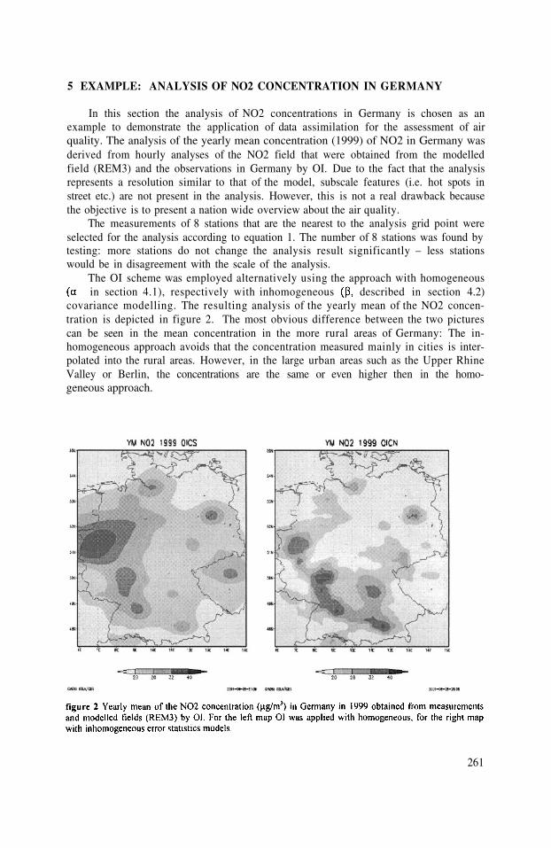
5 EXAMPLE: ANALYSIS OF NO2 CONCENTRATION IN GERMANY
In this section the analysis of NO2 concentrations in Germany is chosen as anexample to demonstrate the application of data assimilation for the assessment of airquality. The analysis of the yearly mean concentration (1999) of NO2 in Germany wasderived from hourly analyses of the NO2 field that were obtained from the modelledfield (REM3) and the observations in Germany by OI. Due to the fact that the analysisrepresents a resolution similar to that of the model, subscale features (i.e. hot spots instreet etc.) are not present in the analysis. However, this is not a real drawback becausethe objective is to present a nation wide overview about the air quality.
The measurements of 8 stations that are the nearest to the analysis grid point wereselected for the analysis according to equation 1. The number of 8 stations was found bytesting: more stations do not change the analysis result significantly – less stationswould be in disagreement with the scale of the analysis.
The OI scheme was employed alternatively using the approach with homogeneousin section 4.1), respectively with inhomogeneous described in section 4.2)
covariance modelling. The resulting analysis of the yearly mean of the NO2 concen-tration is depicted in figure 2. The most obvious difference between the two picturescan be seen in the mean concentration in the more rural areas of Germany: The in-homogeneous approach avoids that the concentration measured mainly in cities is inter-polated into the rural areas. However, in the large urban areas such as the Upper RhineValley or Berlin, the concentrations are the same or even higher then in the homo-geneous approach.
261

6 SUMMARY
In this work data assimilation of ground based concentration measurements into thefields of the Eulerian transport model REM3 was presented. The assimilation is basedon the theoretical framework of Optimum Interpolation. Special emphasis was given tothe modelling of the covariance of the background error and the variance of theobservation error. An new scheme which accounts for the inhomogeneity of theconcentration fields and their measurements was developed. It relies on thediscrimination of air quality regimes in both the observations and the calculated fieldsof the model REM3. The performance of the new approach was compared with that ofthe “standard” homogeneous and isotropic covariance modelling. The new approachleads to more pronounced gradients in the NO2 concentrations, especially to lowerconcentration in rural areas, which seem to be more realistic.
The work should be considered as example to assess air quality by using allavailable information, i.e. observations, model results and climatological studies. Thetechniques of data assimilation are sophisticated tools to combine these informationsources in an objective way. In order to apply these techniques, which were mainlydeveloped for numerical weather forecasting, one has to adapt them to the specificproblems of the air quality measurements as is was done in this work.
7 ACKNOWLEDGEMENTS
This work has been initiated and funded by the German Federal EnvironmentalAgency (Umweltbundesamt) within the project “F+E-Vorhaben 299 43 246”.
8 REFERENCES
Daley, R., 1991, Atmospheric Data Analysis, Cambridge University Press, Cambridge.Egmond Van, N.D. and Onderdelinden, D., 1981, Objective analysis of air pollution monitoring network
data; spatial interpolation and network density, Atmospheric Environment., 15, 1035-1046.Elbern, H., Schmidt H., and A. Ebel, 1997, Variational data assimilation for tropospheric chemisty modeling.
J. Geophys. Res., 102:15967–15985.Falke, S.R. and Husar, R.B., 1998, Declustering in the spatial interpolation of air quality data, in:
Preceedings of the Air & Waist Management Association Annual Meeting, San Diego.Flemming, J., Reimer, E. and Stern, R, 2001, Long Term Evaluation of the Ozone forecast by an Eulerian
Model, Physics and Chemistry of the Earth, to appear.Flemming, J., 2001, Charakterisierung der Messstationen nach dem Immissionsregime, Zwischenbericht zum
UBA FE-Vorhaben 299 43 246, Institut für Meteorologie, Freie Universität Berlin.Gandin, J. L., 1963, The Objective Analysis of Meteorological Fields, Israel Program for Scientific
Translations, Jerusalem.Hass, H., Builtjes, P. J. H., Simpson, D., and Stern, R., 1997: Comparison of model results obtained with
several European regional air quality models, Atmospheric Environment., 31, 3259-3279.Hollingsworth, A. and Lönnberg, P., 1986, The statistical structure of short-range forecast errors as
determined from radiosonde data, Part I: The wind field, Tellus, 38:A, 111-136.Loon van, M. and Heemink, 1997, A.W., Kalman Filtering for non linear atmopsheric chemistry models:
First experiences, Technical Report MAS-R9711, CWI, Amsterdam..Marquardt, D.W. 1963, Journal of the Society for Industrial and Applied Mathematics, vol. 11,pp. 431–441Reimer, E. and Scherer, B., 1992, An operational meteorological diagnostic system for regional air pollution
analysis and long-term modelling, in: Air Pollution Modelling and its Applications IX., van Doop, H..,ed.., Plenum Press.
Stern R, 1994, Entwicklung und Anwendung eines dreidimensionalen photochemischen Ausbreitungsmodells,Meteorologische Abhandlungen Serie A, Band 8, Institut für Meteorologie der FU-Berlin.
262

DISCUSSION
A. HANSEN
J. FLEMMING
E. GENIKHOVICH
J. FLEMMING
P. BUILTJES
J. FLEMMING
In order to avoid imposition of assumptions of isotropy andhomogeneity in your covariance models you might want to lookinto the methodology of Guttorp, Sampson, and Meiering inwhich pollutant fields are mapped into variance space, kriggedand the unmapped back into geographic space. This interpolationis thus done on an isotropic field.
Thank you for your comment.
Using the distance-dependent covariance function, one shouldassume that the field in question is isotropic. Did you test thishypothesis ?
The covariance model presented here is not homogeneous and notisotropic.In the case of the mixing of various covariance functions, theconcepts of isotropy and homogeneity are linked together. This isdue to the fact that the choice of the covariance function (CF)depends on the air quality regime of both grid points. The regimesare distributed according to a long term model calculation.Each single CF represents the hypothetical situation, that onepoint has a certain AQ regime, say urban, and the rest of the fieldhas a different one, say rural. In this sense the CF is isotropic.I do not know how to test the hypothesis of isotropy in this case.
You selected 5 air quality regimes. Are your results sensitive toyour choice, especially for the rural regime ?
We tried to make the classification of air quality parameters asobjective as possible. The classification (hierarchical clustering)ensured stability and homogeneity of the obtained regimes.Although we did not test it systematically – several classificationsgave slightly different results but not in the conclusion that theinhomogeneous covariance model improves the performance ofthe scheme. The rural regime benifited the most. In thehomogeneous case the urban stations “export” their propertiesinto the rural areas.
263

This page intentionally left blank
INCLUSION OF AN IMPROVED PARAMETERISATION
OF THE WET DEPOSITION PROCESS IN AN
ATMOSPHERIC TRANSPORT MODEL
N. Fournier, K.J. Weston, M.A. Sutton, and A.J. Dore *
1. INTRODUCTION
Current pollution models describe the wet deposition of chemical species fromthe atmosphere using the concentration of the species, its scavenging coefficient andthe rainfall rate. However, over the British Isles (BI), the spatial pattern of rainfallintensity often varies on a scale smaller than the spacing between rainfall stations,especially in mountainous areas. Indeed, it is well known that the rainfall rates oc-curing over mountainous and hilly regions are significantly greater than those overthe surrounding low level ground. For the BI conditions, we must take into accountthe orographic enhancement of precipitation and hence wet deposition from theseeder-feeder effect, whereby orographically induced or enhanced clouds over highground (feeder clouds) allow precipitation falling from higher-level clouds (seederclouds) to grow rapidly, giving greater precipitation amounts than over neighbouringlow ground (Bergeron, 1965). The quantitative effects of orographic enhancementover the BI are very dependent on flow direction.
A model of directional orographic enhancement of precipitation is developedwhich incorporates cloudwater generation by orographic and synoptic-scale liftingand the conversion of cloudwater to rainwater (Weston and Roy, 1994). The di-rectional orographic precipitation given by this model is normalised to the BI oro-graphic observed precipitation and incorporated in FRAME through a new param-eterisation of the scavenging coefficients.
*N. Fournier, K.J. Weston, Department of Meteorology, University of Edinburgh, EH9 3JZ,UK. M.A. Sutton, A.J. Dore, Centre for Ecology and Hydrology, Edinburgh Research Station,EH26, UK.
Air Pollution Modeling and Its Application XV, Edited byBorrego and Schayes, Kluwer Academic/Plenum Publishers, New York, 2002 265

Moreover, a more realistic description of the scavenging coefficients is under-taken. Instead of using a fixed value of the height of the atmospheric boundarylayer, a calculated value is considered in the parameterisation. In this paper, wefocus particularly on the United Kingdom (UK) wet reduced-N deposition as allthe UK models underestimate it with respect to available measurements (RGAR,1997).
2. WET DEPOSITION PARAMETERISATION
An atmospheric transport model, FRAME (Fine Resolution AMmonia Ex-change), is used to assess the long-term annual mean surface concentrationand and wet deposition over UK (Singles et al., 1998). Furtherdevelopments extended the domain of the model to the British Isles and improvedits execution time to make more accurate and faster UK estimates (Fournier etal., 2001). FRAME describes the main atmospheric processes (emission, diffusion,chemistry and deposition) taking place in a column of air moving along straight-linetrajectories following specified wind directions.
Wet deposition is the removal of chemical species from the atmosphere throughprecipitation, and is dependent on scavenging, concentration and rainfall rate. Thetwo major mechanisms are in-cloud and below-cloud scavenging. These processescan be modelled using scavenging coefficients, which describe the fraction of theairborne concentration removed per unit time. The amount of material removedin a time period is given by
where is the decrease in concentration of species “i” due to removal by precipi-tation, and is its scavenging coefficient. Most models make no differentiation be-tween in-cloud and below-cloud processes and use an averaged value of the washoutcoefficient to represent the overall effect. Washout coefficients, consistent withthose used in the EMEP model (Tarrason and Schaug, 1999), are combined withrainfall rate to produce appropriate scavenging coefficients. The rainfall data usedare averages for the period 1989-1992 and are in the form of an annual rainfall fieldfor British Isles on a 5km x 5km grid. These data are converted into constant drizzlevalues
A parameterisation of the “seeder-feeder” effect had been previously includedin the model by application of the method proposed by Dore et al. (1992). Forlocations with rainfall less than an assumed sea-level value of
the scavenging coefficient for the species is where is thewashout coefficient for species “i”, P is the precipitation rate Over areaswhere rainfall exceeds it is assumed that this excess rainfall is dueto altitudinal effects, and thus a fraction of the chemical species is removed by theseeder-feeder mechanism. In this case, is calculated by assuming that this excessrainfall will remove twice as much material as normal (enhancement of scavenging
266

coefficients by a factor 2 above the threshold rainfall amount of andthus :
Table 1 shows the United Kingdom 1996 reduced-N deposition budgets obtainedwith this version of FRAME (Run 1). The first column indicates the 1996 estima-tions derived from measurements (NEGTAP, 2001). The model underestimates wetreduced nitrogen deposition, but the dry deposition budget is broadly consistentwith measurements (Fowler et al., 1998). Moreover, the performance of the modelpredictions for wet deposition is illustrated for locations in UK included in theUK National Precipitation Composition Monitoring Network. The model shows areasonable agreement with the 1995 – 97 measurements, but with the model givingsmaller values (slope=0.69 and In this respect, the results of FRAMEare similar to those of other models for the United Kingdom, which all underesti-mate total deposition (RGAR, 1997).
The constant drizzle approach, suitably weighted at each grid square by thefrequency with which each wind direction occurs (British Isles wind rose), does notrepresent the directional-dependence of the enhancement of rainfall over complexorography. Although the seeder-feeder effect is not the only process to produceorographic precipitation in the British Isles (broad-scale up-slope rain, orographicconvective showers and lee-waves (Lee et al., 2000)), it is reasonnable to assumethat the majority of annual rainfall falls as frontal precipitation, in conditions whenthe seeder-feeder effect occurs (Dore et al., 1990; Dore et al., 1992). Therefore, amore physical description of the precipitation over the British Isles is introducedwith the development of a precipitation model.
3. PRECIPITATION MODEL
A model is developed to represent the change of cloud water content in a columnin response to both synoptically and orographically-induced vertical motion (Westonand Roy, 1994). The cloudwater is converted into rainwater by autoconversion. Itcan be summarised by the equations :
267
where is the liquid water content of an air column, its change in moving ahorizontal distance is a threshold value below which no rain occurs, therate of increase of with lifting of the cloud column. is the ground altitudechange over a distance the horizontal speed, the inverse of the time con-stant for conversion of cloudwater to rainwater. P is the precipitation rate andthe non-orographic component of precipitation.
The first term, represents the change in cloudwater due to orographiclifting of the cloud column. Any increase will lead to an increase in precipitationrate and a subsequent depletion of cloudwater content. Therefore, a range of hillswill experience high precipitation, drying out the air stream, so that there is re-duced orographic enhancement over succeeding high ground, or a rain shadow. Thesecond term represents the increase in cloudwater due to large-scale vertical motion.This is related to the rainfall rate upwind of the high ground, The final termrepresents the decrease of cloudwater due to removal as rain. This is assumed tobe proportional to the liquid water content of the cloud column above a thresholdvalue, which converts to rainwater with a time constant of In the model, ifc becomes zero, then any further drying of the air column leaves it under-saturated,so that some further ascent is required before condensation of cloudwater will againtake place. The Weston and Roy (1994) model was applied along straight-line tra-jectories from 24 wind directions in a similar way to those used in FRAME. Theresults are combined statistically, depending on the frequency with which each winddirection occurs and on the percentage of rainfall from each wind direction in rela-tion with the total mean annual rainfall. These latter weighting factors have beendeduced from an analyse of 1985 wind data (K. Weston unpublished data) but arefairly representative of other years. To initialise the precipitation model, severalparameters need to be assigned a value. The values are those used by Weston andRoy (1994) for and Thetrajectories are initialised with an uniform rainfall rate of
The modelled directional orographic precipitation is normalised to the observedorographic precipitation to preserve the total amount of the BI observed long-termaverage precipitation. The observed orographic component is the difference betweenthe total precipitation and its non-orographic component. This non-orographiccomponent is deduced from the observations and the application of a west to eastgradient of 1000 to This new normalised field of precipitation is usedin FRAME where wet and dry periods are combined to quantify the wet reduced-Ndeposition over UK. According to the long-term (1961 – 1990) UK MeteorologicalOffice’s mapped averages, it is assumed that the wet periods represent one third ofthe time of the year.
268

4. SCAVENGING COEFFICIENTS PARAMETERISATION
Parameterisation of scavenging coefficients is the key to the description of thewet deposition process. As a result, particular attention is focused on this parame-terisation. Firstly, the seeder-feeder effect previously developed, is uncorporated inthe model (Run 2, section 4.1). Secondly, the basic parameterisation described insection 2 is improved (Run 3, section 4.2).
4.1 Seeder-Feeder Effect
The seeder-feeder process modifies the local concentrations of ions in precipi-tation because the feeder cloud water, scavenged by falling precipitation, containslarger average concentrations of the major pollutant ions than seeder rain. Thelarger concentrations in hill cloud result from the activation of aerosols contain-ing the pollutants sulphate, nitrate and ammonium into cloud droplets as the airis cooled and force to rise. Thus, the seeder-feeder process leads to a larger in-crease in wet deposition of the major ions with altitude than that of precipitation(RGAR, 1997). A “seeder-feeder” enhancement factor must therefore be appliedto the scavenging coefficients of these ions on the orographic component of precip-itation. A factor of 2 is applied in FRAME following the studies of Fowler et al.(1988), Dore et al. (1992), Inglis et al. (1995) and Fowler et al. (1995). Hence, theparameterisation of the scavenging coefficients becomes :
where is the non-orographic component of the rainfall, is the directionalorographic component of the rainfall (assessed in the previous section). is theenhancement factor, equal to 2 for the ions sulphate, nitrate, ammonium and to 1otherwise.
4.2 Mixing Layer Depth Effect
In the two previous parameterisations of the scavenging coefficients (Eq. (2)and (4)), a fixed depth of the mixing layer was considered. The washout coefficientsin FRAME were consistent with those used in the EMEP model (see section 2)where an air column with a constant depth of 1000 m was assumed. In contrast,in FRAME, the diurnally varying mixing layers profile is calculted depending oninsolation and cloud cover, wind speed and underlying surface. At nighttime, mixinglayer depths are assigned according to Pasquill category and wind speed (Pasquill,1961; ApSimon et al., 1994). The vertical mixing in this mixing layer is thendetermined by the diffusion equation. To improve the physical description of thescavenging coefficients and to be consistent with the diffusion parameterisation, a
269

variable depth of the mixing layer is considered. Eq. (2) can be rewritten :
where is the calculated depth of the mixing layer.
5. RESULTS AND DISCUSSION
The 1996 UK deposition budgets from the different runs with FRAME aregiven in Table 1. There is only a small difference for dry deposited reduced-N be-tween the new parameterisation of the seeder-feeder process in FRAME (Run 2)and the constant drizzle approach (Run 1). In contrast, the different simulationsindicate markedly different UK reduced-N wet deposition.
Run 2, with directional orographic precipitation and an enhancement factorof 2, underestimates the wet deposition from the measurements and from the basicmodel (Run 1) by 59 % and 44 %, respectively. However, with the exception of Scot-land, the general pattern is respected with the highest wet deposition in hill areasof central northern England and Wales. The performance of the model predictionsis illustrated for locations in United Kingdom and the comparison of the modelled
wet deposition from Run 1 with the 1995-97 measurements (RGAR, 1997)shows a correct correlation coefficient but the model is underestimatingthe measurements (slope=0.69). The main discrepancies between the measurementsand Run 1 appear in Scotland; in Wales; in the Pennines; in Yorkshire Moors andin the East of Northern Ireland. The same scatter plot with the modelled wetdeposition obtained from Run 2 gives a similar correlation coefficientbut with a smaller slope (0.30 against 0.69). It is mainly due to a drastic decreaseof wet deposition, in relation with Run 1, in the mountainous areas of thewest coast of the Great Britain facing heavy orographic rainfalls but the air arrivingfrom this direction is relatively clean, in contrast with the east polluted air whichis washed out over England. This pattern of rainfall is more representative of theBritish Isles meteorological conditions than the constant drizzle approach but itsuffers from a limitation of the model which uses straight-line trajectories. Indeed,this approach does not allow air from emission sources to be trapped in cyclonicconditions and so, to come back to a precipitating part of the depression. A betterapproach would be to consider curved trajectories by defining the intensity and thedirection of the wind at each grid point.
Run 3 combines the constant drizzle approach and the use of a variable depthof the mixing layer in the parameterisation of the scavenging coefficients. This ap-proach succeeds to simulate the UK reduced-N wet deposition budget with 106 kt
(Table 1). This close agreement with the estimations derived from measure-ments (110 kt) is confirmed in the comparison of the modelled wet depositionwith the 1995-97 measurements. A slope of 0.83 is obtained with a good correlationcoefficient of 0.64. However, there is still some differences with measurements inScotland, in Wales and in Northern Ireland. The increase of the reduced-N wet
270
deposition budget leads to a decrease of the UK aerosol surface concentra-tion improving the comparison with measurements. Whereas for Run 1 a slope of1.19 was obtained, in Run 3 an improvement is seen with a slope of 1.08
6. CONCLUSIONS
Most precipitation in the BI falls in westerly or southwesterly airflow, as frontalprecipitation, in conditions when the seeder-feeder effect occurs. A model of oro-graphic enhancement of rainfall over the British Isles has been presented. Theprecipitation model can reproduce the main features of the seeder-feeder process,allowing rain-shadows to occur downwind of mountainous areas. Directional oro-graphic precipitation was obtained from this model on a finer spatial scale thanobservations. A seeder-feeder enhancement factor of 2 was applied on this direc-tional orographic precipitation which was then combined with the non-orographiccomponent of the precipitation in FRAME.
The results from FRAME with the new parameterisation were compared with1995-97 measurements. The modelled UK wet deposition underestimates the UKreduced-N wet deposition budget and does not reproduce the peaks present in themountainous regions of Scotland, Wales, Cornwall and the Pennines. These regionsface heavy orographic rainfalls from the west but the air arriving from this directionis relatively clean, in contrast with the east polluted air which is washed out overEngland. Thus, although this parameterisation is more realistic than the previ-ous constant drizzle approach, it suffers from the limitations of the FRAME modelwhich considers straight-line trajectories. This weakness needs to be tackled beforeincorporating such detailed description of the seeder-feeder process.
Nevertheless, the FRAME UK reduced-N wet deposition budget had been im-proved by developing a more realistic description of the scavenging coefficients.The parameterisation combines now the constant drizzle approach with the use ofa variable mixing layer depth leading to a better agreement with measurements.
7. Acknowledgments
Financial support for this work is gratefully acknowledged from the UK NaturalEnvironment Research Council (NERC) and the Department of the Environment,Transport and the Regions, and the Ministry for Agriculture Fisheries and Food.
8.
ApSimon H.M., Barker B.M. and Kayin S. (1994) Modelling studies of the atmospheric releaseand transport of ammonia - applications of the TERN model to an EMEP site in eastern
271
REFERENCES

England in anticyclonic episodes. Atmos. Environ. 28, 665-678.Bergeron T. (1965) On the low-level redistribution of atmospheric water caused by orography. In
Suppl. Proc. Int. Conf. Cloud Physics Tokyo, May 1965, 96-100.Dore A.J., Choularton T.W., Fowler D. and Storton-West R. (1990) Field measurements of wet
deposition in an extended region of complex topography. Q. J. R. Met. Soc. 116, 1193-1212.
Dore A.J., Choularton T.W. and Fowler D. (1992) An improved wet deposition map of the UnitedKingdom incorporating the seeder-feeder effect over mountainous terrain. Atmos. Environ.26A, 1375-1381.
Dore A.J., Choularton T.W., Fowler D. and Crossley A. (1992) Orographic enhancement of snow-fall. Environmental Pollution 75, 175-179.
Fournier N., Pais V.A., Sutton M.A., Weston K.J., Dragosits U., Tang S.Y. and Aherne J. (2001)Parallelisation and application of an atmospheric transport model simulating dispersionand deposition of ammonia over the British Isles. Environmental Pollution (accepted the12 April 2001).
Fowler D., Cape J.N., Leith I.D., Choularton T.W., Gay M.J. and Jones A. (1988) The influenceof altitude on rainfall composition at Great Dun Fell. Atmos. Environ. 22, 1355-1362.
Fowler D., Leith I.D., Binnie J., Crossley A., Inglis D.W.F., Choularton T.W., Gay M., LonghurstJ.W.S. and Conland D.E. (1995) Orographic enhancement of wet deposition in the UnitedKingdom: continuous monitoring. Water, Air and Soil Pollution 85, 2107-2112.
Fowler D., Sutton M.A., Smith R.I., Pitcairn C.E.R., Coyle M., (Campbell G. and Stedman J.)(1998) Regional mass budgets of oxidized and reduced nitrogen and their relative contribu-tion to the N inputs of sensitive ecosystems. Environ. Pollut. (Nitrogen Conference SpecialIssue) 102, S1, 337-342.
Inglis D.W.F., Choularton T.W. and Wicks A.J. (1995) The effect of orography on wet depositionin an industrial area. Q. J. R. Met. Soc. 121, 1575-1588.
Lee D.S., Kingdon R.D., Garland J.A. and Jones M.R. (2000) Parameterisation of the Orographicenhancement of precipitation and deposition in a long-term, long range transport model.Annales Geophysicae 18, 1447-1466.
NEGTAP (2001) Transboundary Air Pollution : Acidification, Eutrophication and Ground-levelOzone in the UK. (First report of the National Expert Group on Transboundary Air Pol-lution), Department of the Environment, Transport and the Regions (DETR), London.
Pasquill F. (1961) The estimation of the dispersion of windborne material. Meteorological magazine90, 33-49.
RGAR (1997) Acid deposition in the United Kingdom 1992-1994. (Fourth report of the UnitedKingdom Review Group on Acid Rain), Department of the Environment, London.
Singles R.J., Sutton M.A. and Weston K.J. (1998) A multi-layer model to describe the atmospherictransport and deposition of ammonia in Great Britain. Atmos. Environ. 32 (3) (AmmoniaSpecial Issue), 393-399.
Tarrason L. and Schaug J. (1999) Transboundary acid deposition in Europe. EMEP report 1/99(July 1999). EMEP- CCC/MSC-W. Norwegian Meteorological Institute, Blindern.
Weston K. J. and Roy M. G. (1994) The directionnal dependence of the enhancement of rainfallover complex orography. Meteorol. Appl, 1, 267-275.
272

DISCUSSIONB. FISHER The changes introduced improve agreement between the
calculated and measured ammonia budget. Measurements of thewet deposition of ammonia tend to be in areas remote from S and
sources but not necessarily ammonia sources. It would beuseful to compare measurements and calculations for sites indifferent regimes e.g. rural sites (near ammonia sources), remotesites (distant from all sources) etc.
N. FOURNIER Two points must be addressed. Firstly, concerning theimprovement in the comparison with measurements, the resultsdiffer depending on the species you consider. and S performwell in contrast with Secondly, following the distribution ofthe sources and measurement sites, the scatter plots betweenmodel and measurements should involve more specifically thedifference between regions of UK.
273

This page intentionally left blank
MODELING OF URBAN AIR POLLUTION:PRINCIPLES AND PROBLEMS
Eugene Genikhovich, Irene Gracheva, and Elena Filatova
1. INTRODUCTION
Urban dispersion modeling (UDM) is usually based on applications of eithernumerical grid models or source-receptor type dispersion models. Numerical dispersionmodels are usually supplemented with numerical “sub-models” simulating the urbanatmospheric boundary layer (UABL). Both types of the models are used to predict thefields of ground-level concentrations (GLC) inside the urban canopy. When analyzingnumerous publications in UDM, one can notice that many of the models have similardeficiencies. In particular, numerical ones frequently do not account for the effect ofblocking up by buildings the volume inside the canopy, which is available for dilution ofpollutants. Corresponding UABL sub-models do not account for the fact that the windspeed, air temperature and other meteorological characteristics should be used only forthe part of this volume, which is free of buildings.
Numerical models, used to simulate the urban air pollution, generate a set ofvalues of concentrations averaged over the grid cells and attributed to some “receptorpoints” located inside these cells, e.g., at their centers. Source-receptor type urbandispersion models also generate a set of concentrations attributed to the receptor point,but they usually do not include any spatial averaging. Actually, these concentrations alsocharacterize a grid cell the size of which is defined by the spacing of the receptorpoints. In both cases one should have certain information about characteristic features ofthe filed to be computed, in particular, the scale of its inhomogeneity, in order tounderstand whether the computed value of concentration can be considered as a good“representative” of all concentrations in the cell. For the most important urban airpollutants, like hydrocarbons and others, is around 20 m, i.e., a characteristicwidth of an urban street (it is known that concentrations at two sidewalks of the samestreet could differ as much as in three times). When mapping the air pollution in the bigcity with a source-receptor type dispersion model and using one can loseimportant features of concentration fields, which simply “fall through” the grid mesh. Asa result, these fields could be grossly misrepresented. Corresponding problems are
Main Geophysical Observatory, 194021, St. Petersburg, Russia
Air Pollution Modeling and Its Application XV, Edited byBorrego and Schayes, Kluwer Academic/Plenum Publishers, New York, 2002 275
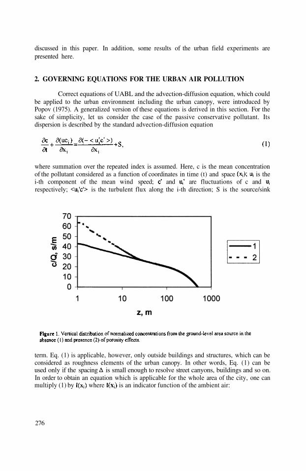
discussed in this paper. In addition, some results of the urban field experiments arepresented here.
2. GOVERNING EQUATIONS FOR THE URBAN AIR POLLUTION
Correct equations of UABL and the advection-diffusion equation, which couldbe applied to the urban environment including the urban canopy, were introduced byPopov (1975). A generalized version of these equations is derived in this section. For thesake of simplicity, let us consider the case of the passive conservative pollutant. Itsdispersion is described by the standard advection-diffusion equation
where summation over the repeated index is assumed. Here, c is the mean concentrationof the pollutant considered as a function of coordinates in time (t) and space is thei-th component of the mean wind speed; and are fluctuations of c andrespectively; is the turbulent flux along the i-th direction; S is the source/sink
term. Eq. (1) is applicable, however, only outside buildings and structures, which can beconsidered as roughness elements of the urban canopy. In other words, Eq. (1) can beused only if the spacing is small enough to resolve street canyons, buildings and so on.In order to obtain an equation which is applicable for the whole area of the city, one canmultiply (1) by where is an indicator function of the ambient air:
276

After averaging, it results in the following equation:
where P is the porosity of the urban canopy which could be defined as a depending onprobability for the receptor point to lie outside the buildings. Accordingly to Popov(1975), P is a result of the averaging over the ensemble of similar cities withidentical buildings stochastically re-distributed inside these cities. Therefore, P dependsonly on the vertical coordinate Such an approach, however, makes impossible anynumerical simulations for a specific city. That is why we assume in this paper that P isdetermined as the moving average of over the area determined by the spacingThus, if P is a smooth function of coordinates. If however, P coincideswith and Eq. (3) is transformed into (1). One should note that in this case P is afunction of all three spatial coordinates and that S is not multiplied by P (because thesources, for example, are located at given point outside buildings).
Similar transformations could be applied, for example, to the first equations ofmotion in UABL:
where is a horizontal component of the drag force due to the interaction of the windflow with obstacles, and the last term in the right-hand side represents the Coriolis force.Other equations of motion are transformed in the same manner. The continuity equationis re-written in the following form:
The same approach can be used to re-formulate the heat transfer-, TKE- and otherequations. It should be stressed out, however, that Eq. (4) and (5) are different from thoseapplied by Popov (he used here).
In the case of the spatially homogeneous city, P depends only on Anexample of the vertical distribution of the normalized concentration, c/Q, from theinfinite area source is given in Fig. 1. Here Q is the specific emission rate from onesquare meter of the source area. It is compared there with a similar distribution in theabsence of porosity effects. The following approximation of function P(z) was used here:
277

where It is seen on Fig. 1 that, due to porosity effects,ground-level concentrations from low sources can be higher than those in the absence ofporosity.
3. MISREPRESENTATION, FILTERING AND REFINEMENT OF URBANCONCENTRATION FIELDS CALCULATED WITH SOURCE-RECEPTORDISPERSION MODELS
When using source-receptor dispersion models, the city area is usually covered with aregular grid mesh so that the concentration fields are “sampled” at regular receptorpoints. Such a sampling at the points that are arbitrarily located relative to the main roadsand other sources resembles the sampling of stochastic time series. In particular, theeffect of alaising (i.e., confounding of frequencies), which is well known in the theory oftime series, is responsible for significant fraction of the errors in computed fields. Here,the wave number corresponding to the grid step plays the role of the Nyquistfrequency. Wave numbers larger than cannot be correctly resolved on the grid. They,however, generate artificial oscillations on this grid with wave numbers less than
278

which, actually, are nothing else but errors. The existing technologies of dispersioncalculations in urban areas usually neglect these features of the concentration fields and,in particular, do not account for the “sampling effects”. As a result, the concentrationscomputed at the regularly spaced grid points do not represent the air pollution incorresponding grid cells. Consequently, the errors in isolines drawn with the use of thecomputed values could be significant.
The effect of misrepresentation of the urban concentration fields with source-receptor type dispersion models could be understood better from calculations for a modelcity. These calculations were carried out with the Russian national regulatory modelOND-86 (see Berlyand et al, 1987; Genikhovich, 1995), which directly generates upper-limit or majorant (actually, percentile) concentration fields. Similar results, however,could be obtained with any other source-receptor dispersion model.
Let us consider four long evenly spaced identical parallel roads, the distancebetween the roads being 2910 m. The origin of the rectangular computational domain islocated on the “left-hand” road, and is the angle between the y-axis of the domain andthe roads. For the sake of simplicity the roads are represented here as the line sources,and concentrations are calculated numerically as integrals along these straight lines fromcorresponding concentrations from the point sources. The majorant concentration fieldfor such a layout calculated with and the grid step m along both, x- and y-
279

directions is shown on Fig. 2. Here, four “ridges” correspond to locations of the roads.Small fluctuations in the values of concentrations along these ridges can be attributed toerrors in the numerical integration. Corresponding isolines are practically parallel to theroads. Numerical tests have confirmed that the same pattern of isolines is generatedwhen doubling the resolution (i.e., when m; in this case the ridges have thesame height but their width is decreased). It should be noted here that this and all othermaps and graphs are mapped with the use of kriging; additional tests were used to provethat the results are not sensitive to interpolation techniques.
One could expect that the pattern of the majorant concentration field should notdepend on orientation of the computational domain. These expectations are not supportedby the results of computations with shown on Fig. 3 (the field there wascomputed with Instead of the ridges, one can see here a kind of a harrowturned upside down. The spikes are attributed to the receptor points located on the roads;they are separated one from another by the areas of low concentrations corresponding toreceptor points off the roads. When doubling the resolution, the number of the spikesincreases twofold but the pattern of the field does not improved but the number of thespikes increases.
The alaising effect is usually eliminated by filtering the oscillations with wavenumbers larger than The simplest way to do it in our case is to average the initial
source-receptor relationships over the length scale In this work, crosswind and along-wind distributions from OND-86 were averaged separately over the same (assuming,therefore, equal steps along x- and y-directions). To avoid writing corresponding bulky280
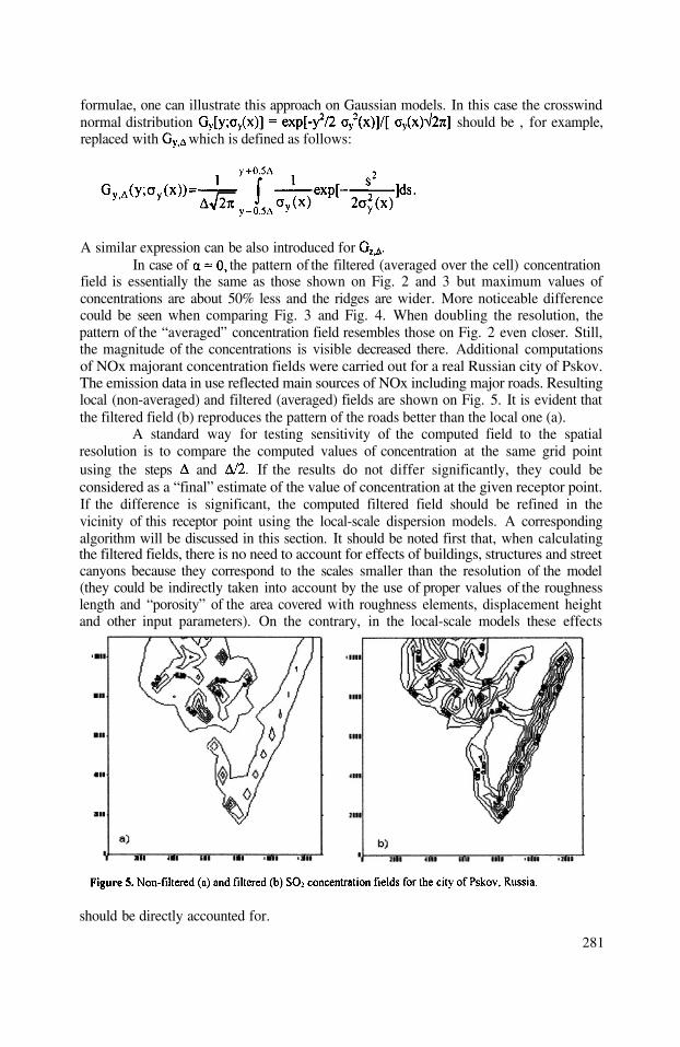
formulae, one can illustrate this approach on Gaussian models. In this case the crosswindnormal distribution should be , for example,replaced with which is defined as follows:
A similar expression can be also introduced forIn case of the pattern of the filtered (averaged over the cell) concentration
field is essentially the same as those shown on Fig. 2 and 3 but maximum values ofconcentrations are about 50% less and the ridges are wider. More noticeable differencecould be seen when comparing Fig. 3 and Fig. 4. When doubling the resolution, thepattern of the “averaged” concentration field resembles those on Fig. 2 even closer. Still,the magnitude of the concentrations is visible decreased there. Additional computationsof NOx majorant concentration fields were carried out for a real Russian city of Pskov.The emission data in use reflected main sources of NOx including major roads. Resultinglocal (non-averaged) and filtered (averaged) fields are shown on Fig. 5. It is evident thatthe filtered field (b) reproduces the pattern of the roads better than the local one (a).
A standard way for testing sensitivity of the computed field to the spatialresolution is to compare the computed values of concentration at the same grid pointusing the steps and If the results do not differ significantly, they could beconsidered as a “final” estimate of the value of concentration at the given receptor point.If the difference is significant, the computed filtered field should be refined in thevicinity of this receptor point using the local-scale dispersion models. A correspondingalgorithm will be discussed in this section. It should be noted first that, when calculatingthe filtered fields, there is no need to account for effects of buildings, structures and streetcanyons because they correspond to the scales smaller than the resolution of the model(they could be indirectly taken into account by the use of proper values of the roughnesslength and “porosity” of the area covered with roughness elements, displacement heightand other input parameters). On the contrary, in the local-scale models these effects
should be directly accounted for.
281
An algorithm of calculation of the refined concentration field could be describedas follows:
1.2.
3.
4.
5.
Run calculations of the filtered concentration with grid steps andFind the receptor points where concentrations are sensitive to variations of thegrid step (i.e., the differences are significant).Find the sources that are responsible for major input into concentration at such areceptor point and sensitive to these variations (“sensitive sources”).Run the local-scale dispersion model for a cell surrounding the given receptorpoint, which is considered as a computation domain, with account for terrainand building effects on dispersion from the sensitive sources.Repeat such a procedure for all receptor points where concentrations aresensitive to variations of the grid step
A computer program based on this algorithm is now under development.
4. CONCLUSION
Results presented in this paper indicate that the technology of urban dispersionmodelling should be corrected in order to account for specific features of the urban airpollution. In particular, the effect of blocking up by buildings the volume inside theurban canopy should be explicitly included in the urban-scale numerical grid models. It isalso important to remember that both numerical and source-receptor type dispersionmodels, when applied in the urban scale, generate values of concentrations which cannotbe considered as “good representatives” of the concentrations in the computational cell.That is why the results of validation of those models upon data of monitoring in the citiesshould be taken with caution.
5. REFERENCES
Berlyand, M.E., Gasilina, N.K., Genikhovich, E.L., Onikul, R.I. and Glukharev V.A. (1987) Method forCalculation of Concentrations of Air Pollutants the Industrial Emissions Contain. National RegulatoryDocument OND- 86. Hydrometeorological Publishers, Leningrad. 92 p.(in Russian)
Genikhovich, E.L. (1995) Practical applications of regulatory diffusion models in Russia.International Journal of Environment and Pollution, vol. 4-5, No 4-6, 530 – 537
Popov, A.M., 1975, On dispersion of pollutants in the urban atmosphere, Meteorology and Hydrology, No 11,p. 48 – 54 (in Russian)
282

DISCUSSION
D. STEYN Can you relate “porosity” to the practical volume of air availablefor pollutant dilution ; and how does porosity depend on depth ofthe urban canopy layer ?
E. GENIKHOVICH The “porosity” could be defined as a fraction of the volume of thegrid cell which is available for dilution. It is, generally speaking,less than 1 inside the urban canopy and equal to 1 outside thecanopy.
A. EBEL The paper is focusing on grid point methods. Would finiteelement methods with better representation of city surface be ableto circumvent the problems of grid point methods ?
E. GENIKHOVICH The proposed approach is used to re-formulate the governingequations. Then they can be solved using different numericaltechniques, finite elements included. I do not think, however, thatfinite elements alone (i.e. “without porosity”) could “reflect” allthe information about the structure and distribution of buildingsinside the urban canopy.
283

This page intentionally left blank
MODELLING CLOUD CHEMISTRY IN A REGIONALAEROSOL MODEL: BULK VS. SIZE RESOLVED
REPRESENTATION
Wanmin Gong*
1. INTRODUCTION
Cloud and aqueous-phase chemistry plays an important role in the production andtransformation of atmospheric aerosol. It is believed that a majority of sulphate aerosolproduction occurs in cloud via aqueous-phase reactions. Historically, cloud processing ofaerosols is considered in the air quality models that deal with acid deposition issues, but isoften represented in a highly simplified and parameterized fashion as most of the modelsonly include gas and bulk aqueous phase and may have some representation of bulkaerosols. With atmospheric particulate matters emerging as a significant human healthhazard in recent years, there is an increased interest to understand not only the bulk massconcentration but also chemical composition and size distribution of the atmosphericaerosols. Air quality models are also beginning to include size- and composition-resolvedaerosols and the various processes affecting their formation and transformation in theatmosphere. However, most of the current regional PM models still adopt a bulkrepresentation for the aqueous-phase chemistry, i.e., assuming that cloud droplets aremonodisperse and homogeneous in chemical composition, for the sake of simplicity andthe consideration of computational burden. On the other hand, there is observationalevidence (e.g. Noone et al., 1988) that the solute concentration in cloud droplets is sizedependent, and studies have shown (e.g. Hegg and Larson, 1990; Roelofs, 1993; Gong,2000) that bulk aqueous-phase chemistry does not resolve the inhomogeneity in chemicalcomposition and pH amongst cloud droplets, which impact on both mass and sizedistribution of cloud processing of aerosols.
A new multiple pollutants (unified) regional air quality modelling system, AURAMS,with size and chemical composition resolved aerosols is being developed (Moran et al.,1998). In the current version of AURAMS a bulk representation of the aqueous-phasechemistry is implemented, as a first step, and is coupled with the size resolved aerosol
* Wanmin Gong, Meteorological Service of Canada, 4905 Dufferin Street, Downsview, Ontario, M3H 5T4,Canada
Air Pollution Modeling and Its Application XV, Edited byBorrego and Schayes, Kluwer Academic/Plenum Publishers, New York, 2002 285

dynamics. One of the objectives of the current study is to assess the impact of bulk versussize-resolved representation of aqueous-phase chemistry on modelled aerosols at aregional scale. In what follows, we will first briefly describe the aqueous-phase chemistrymodule and its implementation in AURAMS; we will present a preliminary examinationof the impact of aqueous-phase chemistry on the modelled regional atmospheric aerosols,based on a simulation of the regional oxidants and aerosols in eastern Canada and the USnorth-east; we will then discuss some results from a test conducted with a stand-aloneversion of the aqueous-phase chemistry module to shed some light on the potential impactof size-resolved versus bulk representation of cloud/aqueous-phase chemistry on aerosolmass production and size distribution.
2. THE CLOUD CHEMISTRY MODULE AND ITS COUPLING WITH SIZE-RESOLVED AEROSOLS
Cloud/aqueous-phase chemistry usually refers to several processes including masstransfer between gas and aqueous-phase (cloud droplets), dissociation/ionisation ofcertain dissolved species and chemical reactions amongst various species in aqueoussolution contained in cloud droplets. The aqueous-phase chemistry mechanism in thepresent study is adapted from ADOM (Acid Deposition and Oxidant Model, Venkatramet al., 1988; Fung et al., 1991). It includes mass transfer of ROOH,
and and oxidation of S(IV) to S(VI) by dissolved ozone, hydrogen peroxide,organic peroxides and oxygen (in the presence of trace metals, e.g. iron and manganese).Mass transfer between gaseous and aqueous phases is treated as a diffusion process, andis written as a set of forward and backward reactions and integrated with the aqueous-phase oxidation reactions. The diffusion coefficients for the mass transfer process aredetermined from Fuchs and Sutugin (1971). The time integration of the chemistry systemis done using a vectorized version of the Young and Boris predictor-corrector solver(Young and Boris, 1977).
The aqueous-phase chemistry is coupled with the explicit aerosol components inAURAMS, namely sulphate, nitrate and ammonium, which are represented by 12 sizebins equally spaced on a logarithmic scale ranging from 0.01 to (Note that aerosolcomponents in the current AURAMS also include organic aerosols and sea-salt aerosols,but they are not directly involved in aqueous-phase chemistry). The nucleationscavenging, which initialises the aqueous phase system, is done through aerosol activationin AURAMS. The aerosol activation is based on an empirical relationship between theaerosol number density and the number density of cloud droplet formed onthe activated aerosols (CCN) described in Jones et al. (1994):
The bulk cloud water content from the meteorological driver model is then distributedevenly amongst the activated aerosols, resulting in a relatively narrow cloud dropletspectrum. The ratios of liquid water content in each activated (or partially activated) sizebins to the total (bulk) cloud water content are used to distribute the bulk mass incrementof the various aerosol components, resulting from the aqueous-phase chemistry, into size
286
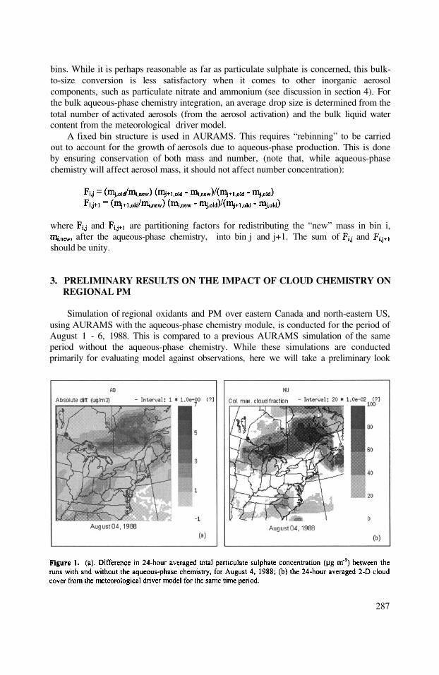
bins. While it is perhaps reasonable as far as particulate sulphate is concerned, this bulk-to-size conversion is less satisfactory when it comes to other inorganic aerosolcomponents, such as particulate nitrate and ammonium (see discussion in section 4). Forthe bulk aqueous-phase chemistry integration, an average drop size is determined from thetotal number of activated aerosols (from the aerosol activation) and the bulk liquid watercontent from the meteorological driver model.
A fixed bin structure is used in AURAMS. This requires “rebinning” to be carriedout to account for the growth of aerosols due to aqueous-phase production. This is doneby ensuring conservation of both mass and number, (note that, while aqueous-phasechemistry will affect aerosol mass, it should not affect number concentration):
where and are partitioning factors for redistributing the “new” mass in bin i,after the aqueous-phase chemistry, into bin j and j+1. The sum of and
should be unity.
3. PRELIMINARY RESULTS ON THE IMPACT OF CLOUD CHEMISTRY ONREGIONAL PM
Simulation of regional oxidants and PM over eastern Canada and north-eastern US,using AURAMS with the aqueous-phase chemistry module, is conducted for the period ofAugust 1 - 6, 1988. This is compared to a previous AURAMS simulation of the sameperiod without the aqueous-phase chemistry. While these simulations are conductedprimarily for evaluating model against observations, here we will take a preliminary look
287

at the impact of aqueous-phase chemistry on modelled regional aerosols (primarilysulphate aerosols). Note that wet removal processes, i.e. cloud-to-rain conversion andscavenging of aerosol particles and soluble gas by falling hydrometeors, are not includedin either of the runs. Therefore this represents somewhat a upper bound as far as the cloudimpact on modelled regional aerosols is concerned. Other processes involving aerosolincluded in the model are nucleation and condensation of sulphuric acid, condensation ofsecondary organic aerosols, coagulation, sedimentation and gravitational removal. (SeeMoran et al., 1998 for a detailed description on the conceptual design of AURAMS).
Figure 1 (a) shows the difference between the two runs in terms of 24-hour averagedtotal particulate sulphate concentration for August 4, 1988 at the ground level.To help with the understanding of the comparison, a 2-D cloud cover (fraction) fieldderived from the 3-D cloud fraction field from the meteorological driver model is shownin Figure 1 (b) for the same 24-hour period. It is seen that there is an increase in totalsulphate aerosol mass concentration as a result of the inclusion of the aqueous-phasechemistry, and, as expected, that the areas with most significant increase in aerosolsulphate closely relate to the areas with most clouds. The enhancement in the modelled24-hour averaged total sulphate aerosol is found up to for this particular day atthis model level. Given that the averaged concentration of the total particulate sulphatefrom the dry run at this level is with maximum concentration of theincrease in sulphate aerosol mass owing to the inclusion of the cloud chemistry issignificant. Overall, the modelled sulphate aerosol mass concentration averaged over thehorizontal domain is increased by about 15% to 50% due to cloud chemistry below 2000m for this one week period. However, the impact of aqueous-phase chemistry on themodelled aerosol will very much depend on the amount of cloud (liquid water) presentand the location of the clouds as well as other atmospheric conditions.
For illustration purpose, Figure 2 shows an example of size distribution of modelledparticulate sulphate from the two runs taken at one grid point at 20 Z August 4, 1988. Itis seen that the main enhancement in particulate sulphate in the run with cloud chemistry
288
is in the 0.3 to range (or bin # 6 - 8 in the model), and that there is a reduction insmaller size bins (bin # 4 and 5). This could be attributed to the growth of smaller aerosolparticles into larger ones due to aqueous phase production. However one should bear inmind that this reflects not only the direct impact of aqueous-phase production but also theindirect interactions between aqueous-phase chemistry and other processes in the model,such as coagulation, sedimentation and gravitational removal.
4. STAND-ALONE TEST ON BULK VS. SIZE-RESOLVED REPRESENTATION
Although a final assessment of the impact of size-resolved vs. bulk representation ofaqueous-phase chemistry on the modelled regional aerosols has to be carried out with a 3-D model, a great deal can be learned from a stand-alone test on the mechanismsresponsible for such impact. In this section we will present some results from an aerosolparcel modelling study (Barth et al., 2001) where a stand-alone version of the currentAURAMS aqueous-phase module was adapted to carry out both bulk and size-resolvedaqueous-phase chemistry simulations.
The simulation is for sulphur oxidation (by dissolved and only) in an airparcel containing initially pure ammonium bisulphate aerosols with a mass concentrationof of and of A log-normal size distribution is specifiedfor the initial aerosols. The parcel is lifted adiabatically with an updraft velocity of 50 cm
Cloud base temperature and pressure are 284.2 K and 939 mb, respectively, and thesimulation is carried out for 40 min, or until the air parcel reaches 1200 m above cloudbase. The initial gas-phase species concentrations are as follows: 200 pptv;100pptv; 500 pptv; 100 pptv, 50 ppbv; 360 ppmv.
Two sets of results will be presented here: one from a size resolved simulation with20 bins covering the range between 0.0014 and (diameter, dry), and the otherfrom a bulk simulation. The time series of temperature, pressure and liquid water contentare obtained from a bulk adiabatic calculation. The empirical aerosol activationformulation (Jones et al., 1994) as in the current AURAMS is used for both simulations,and the bulk simulation is coupled with the initial size distributed aerosols in the samemanner as implemented in AURAMS described in section 2 above.
The final aerosol mass at the end of the 40 minute simulation is compared in Table 1between the two runs. The major difference is in sulphate production - the binned runproduces about 30% more sulphate mass over the 40 minute integration compared to thebulk run. There is no appreciable difference in the production of particulate nitrate andammonium (due to mass transfer, or condensation of and between the tworuns. This is probably due to the way in which bulk water is distributed (equally) amongst
289

the activated aerosols in the binned case, which led to similar drop size and drop number,and therefore the total surface area in the two cases.
Table 2 shows the reduction in and as a direct result of S(IV)-to-S(VI)oxidation in aqueous phase, at the end of the 40-minute integration. The sum of thereductions in and should, in theory, equal that in while the relative size ofthe reductions in vs. indicates the relative importance of the two oxidationpathways. The pH value at the end of the simulation is also shown in Table 2. In the“binned” case, this is an “overall” (or bulk-equivalent) pH weighted by the liquid watercontent in each of the bins. It is seen that, as well as more S(IV) is oxidized to S(VI) inthe “binned” case, the O3 oxidation pathway plays a much more important role in thiscase than the bulk run (i.e. 42% in the binned run as opposed to 21% in the bulk run).Nonetheless the pH values from the two cases are quite similar! However, by looking atthe results from the binned run a little more closely, we quickly realise that the “overall”pH does not represent well what happens in each individual bins. Figure 3 is a plot of afew pH time series for the 40-minute simulation. The pH from the bulk run, the overallpH, and the pH for bin #10 and #11 from the binned run are shown. These two bins are atthe smaller end of the size spectrum which are activated. As seen, while the overall pHfrom the binned run compares closely with the one from the bulk run, the pH values forthe activated bins that contain originally smaller particles are significantly higher, whichwould enable to play a much more important role in the aqueous-phase S(IV)oxidation. The lower acidity in these bins in the simulation is due to the fact that an equalamount of liquid water is distributed to all the activated aerosol particles in the model.However this may not be unexpected in the real world as it is known that the condensationof water vapour on smaller particles/drops is much faster than to the larger ones.
290

Therefore droplets grown from originally smaller particles can be much more dilute thanthose grown from the larger ones. However, this needs to be investigated further, ideallywith a size-resolved aerosol model with fully coupled cloud microphysics and chemistry.
Another issue of interest is the impact of bulk vs. size resolved aqueous-phaserepresentation on modelled aerosol size distribution. Figure 4 shows the size distributionof sulphate and ammonium aerosols at the end of the 40-minute integration from the tworuns. In the case of the bulk run, the bulk-to-size conversion is done in the same way asin current AURAMS (see section 2). It is seen that for sulphate the distributions from thetwo runs are not too different particularly after rebinning. The binned run is seen toproduce a double peak distribution (over bins) before rebinning, with a first peak centredat bin 11, while the bulk run does not show the same feature. This is a result of theenhanced sulphur oxidation in the smaller activated bins due to the enhanced role of O3 inthe oxidation in the case of the binned run. The difference between the two runs is moresignificant in the distribution of ammonium aerosols. “Off-gassing” from larger size binsis clearly seen from the binned run, while it is not reflected in the bulk run since the bulk-to-size conversion is done using liquid water distribution. The difference is lesssignificant after the rebinning.
5. CONCLUSIONS
A number of points can be made from the current study. Firstly, aqueous-phasechemistry is shown to have a significant impact on the modelled regional aerosols. It notonly enhances aerosol production but also alters aerosol size distribution, which willfurther affect other aerosol processes (e.g. coagulation, sedimentation and gravitationalremoval etc.). The degree of this impact depends strongly on the presence of cloud, theamount of cloud water, its geophysical distribution and other atmospheric conditions.
291
It is seen, from the stand-alone test, that a size-resolved representation in aqueousphase oxidizes more sulphur than a bulk representation. This is in agreement withprevious findings. The present study seems to indicate that the enhancement is a result ofinhomogeneity in acidity (or solute concentration) amongst activated aerosols (drops).The drops originated/activated from the initially smaller aerosol particles are more dilutewith lower acidity which are responsible for the enhanced S(IV) oxidation by aqueous-phase The bulk representation has another problem of regenerating the sizedistribution when coupled with size-resolved aerosols. Although it seems to workreasonably well for the sulphate aerosol component, the current scheme for bulk-to-sizeconversion does not work as well for other aerosol components, such as nitrate andammonium, where “off-gassing” from larger size bins (or drops with higher soluteconcentration) will be difficult to represent with a bulk formulation.
Finally, a few things need to be pointed out as a caution. Particularly, the test on bulkvs. size-resolved chemistry presented here mainly addresses the issue of chemicalinhomogenneity amongst cloud drops, and is influenced by the rather crude activationscheme and the distribution of bulk cloud water to activated aerosol particles used in thestudy. It would be more desirable to integrate the size-resolved chemistry with size-resolved cloud microphysics. However, this is still rather formidable to realise in 3-Dregional scale models.
ACKNOWLEDGEMENT
Dr. V. Bouchet of MSC provided the results from the simulation with the “dry version” ofAURAMS. Mr. S. Menard (now at CMC/MSC) provided programming support for theimplementation of the cloud chemistry module in AURAMS.
REFERENCE
Barth, M.C., S.M. Keidenweis and R. Hudman, 2001. Comparison of cloud chemistry and aerosol parcelmodel simulations. To appear in WMO report on the International Cloud Modelling Workshop, Aug 7- 11, 2000, Glenwood Springs, Colorado.
Fuchs, N.A. and A.G. Sutugin, 1971. Highly dispersed aerosols. In Topics in Current Aerosol Research, Vol.2, G.M. Hidy and J.R. Brock, Editors, Pergamon Press,, New York, 1-60.
Fung, C.S., P.K. Misra, R. Bloxam and S. Wong, 1991. A numerical experiment on the relative importance ofH2O2 and O3 in aqueous conversion of SO2 to SO42-, Atmos. Environ., Vol. 25A, No. 2, 411-423.
Gong, W., 2000. Bulk vs. size-resolved representations in modelling mass transfer and aqueous-phasechemistry in cloud droplets in regional models. Preprint volume of the 11th Joint Conference on theApplication of Air Pollution Meteorology with the A&WMA, 376-378.
Hegg D. A. and T. V. Larsen, 1990. The effects of micro-physical parameterization on model predictions ofsulphate production in cloud. Tellus, 42B, 272-284, 1990.
Jones, A., D.L. Roberts, and J. Slingo, 1994: A climate model study of indirect radiative forcing byanthropogenic sulphate aerosols, Nature, 370, 450-453.
Moran, M. D., A. P. Dastoor, S.-L. Gong, W. Gong and P. A. Makar, 1998. Conceptual design for the AESunified regional air quality modelling system. Air Quality Research Branch, Meteorological Service ofCanada, Downsview, Ontario M3H 5T4, Canada.
Noone, K. J., R. J. Charlson, D. S. Covert, J. A. Ogren and J. Heintzenberg, 1988. Cloud droplets soluteconcentration is size dependent. J. Geophys. Res., 93, 9477-9482.
Roelofs, G.J.H., 1993. A cloud chemistry sensitivity study and comparison of explicit and bulk cloud modelperformance. Atmos. Environ. 27A, 2255-2264.
292

Venkatram, A., P.K. Karamchandani and P.K. Misra, 1988. Testing a comprehensive acid deposition model.Atmos. Environ., 22, 737-747.
Young T.R. and Boris J. P., 1977. A numerical technique for solving stiff ordinary differential equationsassociated with the chemical kinetics of reactive-flow problems. J. Phys. Chem. 81, 2424-2427.
293

This page intentionally left blank
PARAMETERIZATION OF TURBULENCE–ENHANCEDNUCLEATION IN LARGE SCALE MODELS:
CONCEPTUAL STUDY
Olaf Hellmuth and Jürgen Helmert1
1. INTRODUCTION
Binary homogeneous nucleation of sulfuric acid and water vapor has longbeen suspected to be an important mechanism for new particle formationin the atmosphere (e. g., Stauffer, 1976). Nucleation is a highly nonlinearprocess, which is very sensitive to spatial and temporal variability. Owing tothe coarse vertical and horizontal resolution, and rather long integration timesteps in large scale models, unresolved subgrid-scale processes must be pa-rameterized. Easter and Peters (1994) evaluated the effect of turbulent-scalevariations on the binary nucleation rate. They found an enhancement factor,that is, the ratio of the nucleation rate in the presence of turbulence-scalefluctuations to that at mean-state conditions, of up to for anticorrelatedtemperature and humidity fluctuations.
1 Olaf Hellmuth and Jürgen Helmert, Institute for Tropospheric Research Leipzig, Per-moserstr. 15, Leipzig, D–04303, Germany
Air Pollution Modeling and Its Application XV, Edited byBorrego and Schayes, Kluwer Academic/Plenum Publishers, New York, 2002 295
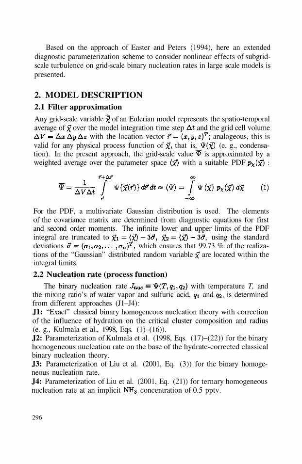
Based on the approach of Easter and Peters (1994), here an extendeddiagnostic parameterization scheme to consider nonlinear effects of subgrid-scale turbulence on grid-scale binary nucleation rates in large scale models ispresented.
2. MODEL DESCRIPTION2.1 Filter approximation
Any grid-scale variable of an Eulerian model represents the spatio-temporalaverage of over the model integration time step and the grid cell volume
with the location vector analogeous, this isvalid for any physical process function of that is, (e. g., condensa-tion). In the present approach, the grid-scale value is approximated by aweighted average over the parameter space with a suitable PDF
For the PDF, a multivariate Gaussian distribution is used. The elementsof the covariance matrix are determined from diagnostic equations for firstand second order moments. The infinite lower and upper limits of the PDFintegral are truncated to using the standarddeviations which ensures that 99.73 % of the realiza-tions of the “Gaussian” distributed random variable are located within theintegral limits.
2.2 Nucleation rate (process function)
The binary nucleation rate with temperature T, andthe mixing ratio’s of water vapor and sulfuric acid, and is determinedfrom different approaches (J1–J4):J1: “Exact” classical binary homogeneous nucleation theory with correctionof the influence of hydration on the critical cluster composition and radius(e. g., Kulmala et al., 1998, Eqs. (1)–(16)).J2: Parameterization of Kulmala et al. (1998, Eqs. (17)–(22)) for the binaryhomogeneous nucleation rate on the base of the hydrate-corrected classicalbinary nucleation theory.J3: Parameterization of Liu et al. (2001, Eq. (3)) for the binary homoge-neous nucleation rate.J4: Parameterization of Liu et al. (2001, Eq. (21)) for ternary homogeneousnucleation rate at an implicit concentration of 0.5 pptv.
296

2.3 First order moments
The grid-scale profiles of are usually available from the large scalemodel. For the conceptual study presented here, these profiles are deriveddiagnostically from similarity theory of the convective boundary layer (CBL)(Stull 1997, p. 368–374).
Temperature: The vertical gradient of the temperature and potentialtemperature reads as:
In (2), is the surface layer (SL) similarity function for nonzero surfacestress, and the mixed layer profile function. The temperature gradientat the CBL top is and and are the kinematic and convectivetemperature scale related to the SL heat fluxwith the kinematic and convective velocity scalesFurthermore, L is the Monin-Obukhov length, the dimensionlessheight, the standard deviation of the vertical velocity, andthe dry adiabatic temperature lapse rate.
Humidity, acidity: The vertical gradient of the water vapor mixing ratioreads as:
Here, and are the kinematic and convective water vapor mixingratio scales, related to the SL humidity flux Itis determined from the Bowen ratio for given SL heat flux. The water vaporpartial pressure results from The sulfuric acid vapor pressure
is assumed to be in constant ratio to the water vapor pressure, preset inthe surface layer, that is, with = const..
Wind: Rotating the coordinate system to align the wind direction with thethe vertical gradient of wind velocity is given as:
Here, is the vertical wind gradient at the CBL top.
297

2.4 Second order moments
Heat flux: The heat flux results from the heat flux equation under hor-izontally homogeneous and quasi-steady state conditions with Boussinesqapproximation (Holtslag and Moeng, 1991, Eqs. (1)–(8)):
Here, is the eddy diffusivity for heat, an empirical parameters forCBL turbulence.
Turbulent kinetic energy (TKE): The prognostic equation for the TKEof a horizontally homogeneous Boussinesq fluid (Therry and Lacarrère, 1983)reads as:
Here, and are the density and potential temperature of air at the refer-ence state, and is the buoyancy parameter. The terms on the r.h.s.describe respectively vertical diffusion, shear production, buoyancy produc-tion and viscous dissipation. The vertical turbulent fluxes of momentum andheat and the TKE diffusivity term are parameterized as
with the countergra-dient term and the eddy diffusivities for momentum, heat and TKE
Here, (recip-rocal of the turbulent Prandtl number), and The dissipation rateis parameterized as with the dissipation length scale andthe dissipation parameter Inserting the previous parameterizations into(6), we obtain for the quasi-steady state, the following diagnosticequation:
Temperature and humidity variance: The variance equation for thetemperature and water vapor mixing ratio with of ahorizontally homogeneous Boussinesq fluid (André et al., 1978) reads as:
298

Inserting the parameterizations of the turbulent fluxesonly for the turbulent transport terms
and the dissipation terms withand into (8), we obtain the following diagnostic
equation for steady-state conditions,
The standard deviation of the temperature and the sulfuric acid mixing ratioreads as and
2.5 Miscellaneous
Boundary conditions: At the lower boundary with SLheight the TKE is determined usingempirical variances of wind velocity. The temperature variance
results from and the humidityvariance from
At the upper boundary the TKE reads as
resulting from CBL top heat flux with heatflux ratio andThe gradient of the temperature variance
is derived from CBL measurements, that is,(198… 330) (Caughey and Palmer, 1979, Fig. 5),
and that of the humidity variancefrom humidity variances for Day 33, Wangara (Stull 1997, p. 129,
Fig. 4.7) , that is,
Length scales: The characteristic turbulence length scale is parameterizedas derived from LES of aCBL (Hellmuth and Helmert, 2001, subm.). For peak wavelength of thevertical velocity spectrum in the CBL is used,
which is related to the dissipation rate, with(Caughey and Palmer, 1979). With
and we have
Velocity variances: In (2), (3), (5), and to determine and parame-terized velocity variances are used (Kerschgens et al., 2000, Eq. (4.1)).
299
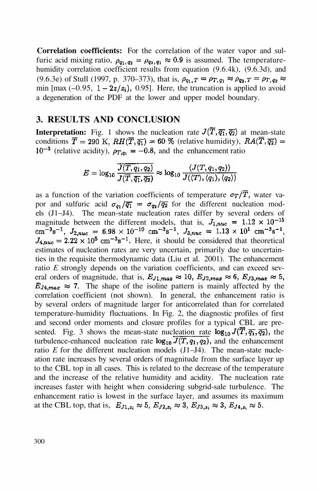
Correlation coefficients: For the correlation of the water vapor and sul-furic acid mixing ratio, is assumed. The temperature-humidity correlation coefficient results from equation (9.6.4k), (9.6.3d), and(9.6.3e) of Stull (1997, p. 370–373), that is,min [max (–0.95, 0.95]. Here, the truncation is applied to avoida degeneration of the PDF at the lower and upper model boundary.
3. RESULTS AND CONCLUSIONInterpretation: Fig. 1 shows the nucleation rate at mean-stateconditions (relative humidity),
(relative acidity), and the enhancement ratio
as a function of the variation coefficients of temperature water va-por and sulfuric acid for the different nucleation mod-els (J1–J4). The mean-state nucleation rates differ by several orders ofmagnitude between the different models, that is,
Here, it should be considered that theoreticalestimates of nucleation rates are very uncertain, primarily due to uncertain-ties in the requisite thermodynamic data (Liu et al. 2001). The enhancementratio E strongly depends on the variation coefficients, and can exceed sev-eral orders of magnitude, that is,
The shape of the isoline pattern is mainly affected by thecorrelation coefficient (not shown). In general, the enhancement ratio isby several orders of magnitude larger for anticorrelated than for correlatedtemperature-humidity fluctuations. In Fig. 2, the diagnostic profiles of firstand second order moments and closure profiles for a typical CBL are pre-sented. Fig. 3 shows the mean-state nucleation rate theturbulence-enhanced nucleation rate and the enhancementratio E for the different nucleation models (J1–J4). The mean-state nucle-ation rate increases by several orders of magnitude from the surface layer upto the CBL top in all cases. This is related to the decrease of the temperatureand the increase of the relative humidity and acidity. The nucleation rateincreases faster with height when considering subgrid-sale turbulence. Theenhancement ratio is lowest in the surface layer, and assumes its maximumat the CBL top, that is,
300
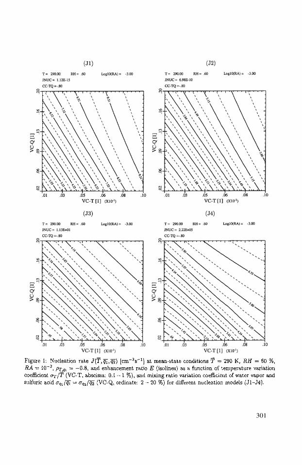
301

302

303

Conclusion: Second order statistics provide useful information for the pa-rameterization of the influence of subgrid-scale variations on the spatio-temporal average of the nucleation rate. In large scale models, the nucleationenhancement due to subgrid-scale turbulence can lead to nucleation events ingrid cells with weak mean-state preconditioning for new particle formation.The effect is comparable to the effect of hydration of sulfuric acid as well asto the contribution of ammoniac in nucleation (Korhonen et al., 1999, Fig. 2).The results also show, that the upper part of the CBL is a favoured place ofnew particle formation. Considering the growth time of the critical nucleusto a detectable size, which is in the order of the large eddy turn over time,observed nucleation events in the surface layer are easily possible to resultfrom top-down diffusion of faster formed new particles at the CBL top.
REFERENCESAndré, J. C., G. De Moor, P. Lacarrère, G. Therry, and R. Du Vachat, 1978: Modeling
the 24-hour evolution of the mean and turbulent structures of the planetary boundarylayer. J. Atmos. Sci., 35, 1861–1883.
Caughey, S. J., and S. G. Palmer, 1979: Some aspects of turbulence structure through thedepth of the convective boundary layer. Quart. J. Roy. Meteor. Soc., 105, 811–827.
Easter, R. C., and L. K. Peters, 1994: Binary homogeneous nucleation: Temperature andrelative humidity fluctuations, nonlinearity, and aspects of new particle production inthe atmosphere. J. Appl. Meteor., 33, 775–784.
Hellmuth, O., and J. Helmert, 2001: Length scale determination using large-eddy simula-tion of the convective boundary layer. Meteorol. Z., Subm.
Holtslag, A. A. M., and C.-H. Moeng, 1991: Eddy diffusivity and countergradient transportin the convective atmospheric boundary layer. J. Atmos. Sci., 48, 1690–1698.
Kerschgens, M., C. Nölle, and R. Martens, 2000: Comments on turbulence parametersfor the calculation of dispersion in the atmospheric boundary layer. Meteorol. Z., 9,155–163.
Korhonen, P., M. Kulmala, A. Laaksonen, Y. Viisanen, R. McGraw, and J. Seinfeld, 1999:Ternary nucleation of and in the atmosphere. J. Geophys. Res.,104, 26,349–26,353.
Kulmala, M., A. Laaksonen, and L. Pirjola, 1998: Parameterizations for sulfuric acid/water nucleation rates. J. Geophys. Res., 103, 8301–8307.
Liu, X., D. A. Hegg, and M. T. Stoelinga, 2001: Numerical simulation of new particleformation over northwest Atlantic using MM5 mesoscale model coupled with sulfurchemistry. J. Geophys. Res., 106, 9697–9715.
Stauffer, D., 1976: Kinetic theory of two-component (“heteromolecular”) nucleation andcondensation. J. Aerosol Sci., 7, 319–333.
Stull, R. B., 1997: An Introduction to Boundary Layer Meteorology. Kluwer AcademicPublishers, Dordrecht/ Boston/ London.
Therry, G., and P. Lacarrère, 1983: Improving the eddy kinetic energy model for planetaryboundary layer description. Boundary-Layer Meteor., 25, 63–88.
304

DISCUSSION
P. BUILTJES
O. HELLEMUTH
Many parameters and correlation coefficients are needed to performyour correlation. Is it possible to determine them experimentally, forexample the correlation between water vapour and temperature ?
In principle, all elements of the PDF covariance matrix could be
obtained by using additional forecast equations, i.e. for
etc. For practical reasons, the present approach has
been limited to the determination of the variances only, that is
The cross-correlation coefficients of temperature
and water vapor mixing ratio can be obtained from measurements,even they are scarce and highly uncertain. The most importantproblem is the determination of water vapor – sulfuric acid crosscorrelation due to the problem of getting highly time resolvedsulfuric-acid measurements. The same is true for temperature –sulfuric acid cross correlation. A suitable way to overcome allsampling problems might be the use of LES to parameterize allcross-correlation terms as function of scaling properties (mixinglayer height, Monin-Obukhov length and convective temperature,velocity, humidity, and concentration scales …).Before such an approach is performed, the sensitivity of the aerosolevolution on the turbulence-enhanced nucleation rate should beinvestigated in a large and/or mesoscale model.
305

This page intentionally left blank

MODELS-3/COMMUNITY MULTISCALE AIRQUALITY (CMAQ) MODELING SYSTEM
2001 Java-based release
Sharon LeDuc and Steven Fine*
1. INTRODUCTION
The U.S.E.P.A. has developed the Models-3/CMAQ (Community Multiscale AirQuality) modeling system, with the initial release occurring during 1998. EPA/NOAAscientists and their colleagues are continuously striving to improve and to evaluate thescientific basis and the scientific algorithms in CMAQ. In addition, they are working toprovide and improve the Models-3 framework to provide a user-friendly interface for airquality modeling. The application and functionality of an earlier version (version 3) ofModels-3/CMAQ was presented at the Millennium NATO/CCMS InternationalTechnical Meeting on Air Pollution Modelling and Its Application (LeDuc et al., 2000).This paper briefly describes Version 4.1, released during early 2001, and Version 5,scheduled for a November 2001 release. The November 2001 release will have an entirelynew framework which has been designed to be extensible for cross-media modeling (air,water, soil, vegetation, exposure and risk) of pollutants. This is part of a new modeling effortis known as MIMS, Multimedia Integrated Modeling System, which is a multi-year effort byU.S.E.P.A. Air quality modeling is the first Amedium@ to be modeled in MIMS. Thescience used for that modeling has evolved from the Models-3/CMAQ modeling system. TheNovember 2001 release will incorporate the Modified Euler Backward Iterative (MEBI)solver for selected gas-phase chemical mechanisms. The solver is considerably faster thanthe Quasi-Steady State Approximation Method and the Sparse-Matrix Vectorized Gearsolver. Previous changes to Models-3/CMAQ will be presented along with the expectedcapability of the MIMS framework which will contain the latest version of Models-3/CMAQmodeling system.
* Atmospheric Sciences Modeling Division, Air Resources Laboratory, National Oceanic and AtmosphericAdministration, on assignment to National Exposure Research Laboratory, U.S. Environmental ProtectionAgency, MD-80, Research Triangle Park, North Carolina 27711, U.S.A.
Air Pollution Modeling and Its Application XV, Edited byBorrego and Schayes, Kluwer Academic/Plenum Publishers, New York, 2002 307

2. MODELS-3/CMAQ VERSION 4.1
The Models-3/CMAQ version 4.1 was released during the period February thru August2001. A description of that system (Byun et al., 2001) indicates the status of the science,including the emissions processor the Sparse Matrix Operator Kernel Emissions (SMOKE)modeling system from MCNC, North Carolina Supercomputing Center’s EnvironmentalPrograms (MCNC, 2001). Both SMOKE and SMOKE Tool (Atmospheric ModelingDivision et al., 2001) are integrated into version 4.1 of the framework. The latest version ofSMOKE has new features for enhancing the quality assurance capability (Houyoux andAdelman, 2001). Science codes and scripts to execute all processing, referred to as aAstandalone@ version, are available for downloading from the Models-3 website (EPA,2001b) for three computing platforms: Sun, SGI and Windows NT. Users have adapted thesefor other computing platforms, e.g. DEC Alpha and Linux. This standalone version is codedto execute a tutorial situation. Users will need to do additional processing for executinganother geographic domain, using an alternate chemical mechanism, or simulating anothertime period. All components including SMOKE and SMOKE Tool will execute without theframework.
The framework assists users in setting up the domain and executables for simulating acase beyond the tutorial. The framework has been released for the Sun workstation and forthe Windows NT computing platforms. The framework requires users to purchase severalproprietary software packages (SAS and ARC/INFO) for the emissions processing, and aruntime license for the object-oriented communications software. For the Windows NTgraphics, the user must also purchase and install software for PC X connectivity, e.g.Hummingbird Exceed, and the unix emulation software Interix. One graphic package thatis in Version 4.1 and that will be integrated into the framework is PAVE (Thorpe et al.,1996), which may be downloaded (MCNC, 2001).
3. PLANS FOR NOVEMBER 2001 RELEASE
The November 2001 release will include a new framework being developed forU.S.E.P.A.=s Multimedia Integrated Modeling System (MIMS). Design details of theframework are available at the MIMS website (EPA, 2001a). This release will replace theold Models-3 framework. The Amultimedia@ to be modeled in the MIMS system are themultiple physical media, such as air, water, and soil. The new MIMS framework will makeit easier to configure and execute complex modeling studies. For instance, the newframework will provide facilities for easily re-executing model configurations with differentdata sets. This is a commonly needed capability, especially to simulate multiple episodes.
The MIMS framework has been designed to be portable across platforms and to requireno software that will incur a cost for the end user. The model communication paradigm inMIMS is based on the Dynamic Information Architecture System (DIAS), a flexible object-based software framework that provides the structure and flexibility required to successfullyinterchange models of very diverse processes (Christiansen, 2000). The MIMS frameworkis being developed in Java, which provides portability across platforms. None of the third-
308

party libraries that are used have a distribution fee. Documentation for the MIMS frameworkwill be in the form of both JavaHelp (a cross-platform hypertext help system) and hardcopy.As a result of all of these charateristics, the MIMS framework will be much easier for a user
to obtain, install, and use than the Models-3 framework through Version 4.1.The development and testing of the new framework has been accomplished with
cooperation between the air quality modeling scientists and the software developers. Theaddition of features and functionality has been directed by a voting process followingprinciples of Extreme Programming (Beck, 2000), which recommends a softwaredevelopment approach with a high degree of input and feedback from users. Additionalfeatures will be included in the November release, but because the last round of voting hadnot occurred at the time this paper was prepared, those high priority features were not known.
Major advancements in the models= functionality and capability in the November 2001release are made possible by the use of Fortran 90 and dynamic allocation. This will enableusers to change options, such as the geographic domain and the number of vertical layers,without recompiling. A windowing capability will allow extraction of subareas from largerdomains. Users will have the ability to edit the chemical mechanism in the framework,although this should be used cautiously by knowledgeable users. SMOKE will be integratedinto the framework which will be released in November, however, users will be expected todownload it separately (MCNC, 2001).
Modular spatial allocation routines written in Fortran 90 will replace much, if not all, ofthe ARC/INFO functionality. It is questionable, however, whether or not the requirement forARC/INFO can be dropped. As mentioned before, PAVE will be also included in theNovember release.
The November release will have new science features. The Biogenic EmissionsInventory System version 3 (BEIS3) will be included for simulating biogenic emissions inSMOKE. [It is unlikely that Mobile6 will be available in time to include in the Novemberrelease.] The State Air Pollution Research Center (SAPRC) chemical mechanism will beincluded and the Modified Euler Backward Iterative (MEBI) solver will be expanded toprocess the Regional Acid Deposition Model version 2 (RADM2) chemical mechanism.Emissions will be processed in the vertical diffusion processing instead of in the chemistryprocessing as was done in earlier versions. The Plume-IN-Grid (PING) will be extended toinclude an aerosol processing capability. Atrazine emissions will be processed in CMAQ.MM5 version 3 output will be able to be processed by the meteorology chemistry interface
processor (mcip). The emissions chemistry interface processor (ecip) is no longer neededwith SMOKE.
The air quality modeling community recognizes the need to continue to improve thescience and understanding used by models. The modeling results are used to make decisionsthat will influence future air quality. The science must be as correct and complete aspossible. A modeling user-friendly modeling framework that will execute on a widespectrum of computing platforms, and that does not require extensive, continuing softwarecosts will make the air quality modeling available to a broad population of users. The Java-based release of Models-3/CMAQ intends to provide these capabilities in November2001.
309

4. DISCLAIMER
This paper has been reviewed in accordance with the U.S. Environmental ProtectionAgency=s peer and administrative review policies and approved for presentation andpublication. Mention of trade names or commercial products does not constituteendorsement or recommendation for use.
5. REFERENCES
Atmospheric Modeling Division, National Exposure Research Laboratory and EPA Systems Development Center,2001, SMOKE Tool for Models-3 version 4.1: structure and operation documentation, EPA-600/R-01/04.
Beck, K., 2000, Extreme Programming Explained, Addison-Wesley, Reading, Massachusetts.Byun, D., Benjey, W., Binkowski, F., Ching, J., Dennis, R., Eder, B., Gipson, G., Godowich, J., Lacser, A., LeDuc,
S., Novak, J., Otte, T., Pierce, T., Pleim, J., Roselle, S., Schere, K., Young, J., Jang, C., Gillani, N., Biazar, A.,Hanna, A., Coats, C., McHenry, J., Mathur, R., Shankar, U., Xiu, X., Odman, T., Tang, R., Wong, D. andBourgeois, A., 2001, Description of Models-3/Community Multiscale Air Quality (CMAQ) model: systemoverview, governing equations, and science algorithms, EPA internal report.
Christiansen, J.H., 2000, A flexible object-based software framework for modeling complex systems with interactingnatural and societal processes, in: International Conference on Integrating GIS and Environmental Modeling(GIS/EM4): Problems, Prospects and Research Needs, Banff, Alberta, Canada, September 2-8, 2000.
EPA, 2001a, North Carolina,http://www.epa.gov/asmdnerl/mims/index.html.EPA, 2001b,North Carolina, http://www.epa.gov/asmdnerl/models3/announce. html.Houyoux, M. R. and Adelman, Z, 2001, Quality Assurance Enhancements to the SMOKE Modeling System, in: The
Emission Inventory Conference: One Atmostphere, One Inventory, Many Challenges, 1-3 May, Denver, CO,U.S.Environmental Protection Agency.
LeDuc, S.K., Schere, K.L., Godowich, J.M. and Gipson G.L., 2001, Models-3/CMAQ Applications Which IllustrateCapability and Functionality, in: Air Pollution Modeling and Its Application XIV, S.-E. Gryning and F.A.Schiermeier., ed., Kulwer Academic/Plenum Publishers, New York, pp.737-738.
MCNC, 2001, North Carolina, http://envpro.ncsc.org/products/.Thorpe, S., Ambrosiano, J., Coats, C., Eyth, A., Fine, S., Hils, D., Smith, T., Trayanov, A., Balay, R, Vouk, M.,
Turner, T., 1996, The Package for Analysis and Visualization of Environmental Data. Proc., Computing inEnvironmental Resource Management, 2-4 December, Research Triangle Park, NC, Air & Waste ManagementAssoc., 241-249.
310
FUZZY SETS APPLICATIONFOR ESTIMATION OF AIR POLLUTED ZONE
Andry A. Dudatiev, Yuliya Y. Podobna, Pavlo A. Molchanov and Tatyana G.Holyeva*
1. INTRODUCTION
When the forecast of scales of pollution is realized directly after failure the concrete dataabout the amount of ejected SAPS (strongly affecting poisonous substances) and actualmeteorological conditions are accepted (Ukraine Stuff of Civil Defense, 1999).
Generally, the area covered by a pollution zone consists of two parts:The equivalent amounts of poisonous substances in the primary and the secondary cloudsare determined.
The special table determines radiuses of pollution zones by the primary and the secondaryclouds, accordingly and The full depth of a pollution zone, is stipulated by influenceof the primary and the secondary SAPS clouds determined as follows:
where G is the full depth of a pollution zone, G ” is the largest radius of pollution, G ’ is thesmallest radius of pollution.
In case of absence of accurate basic data about the influencing factors, the forecast of possibleconsequences is carried out using given parameters of meteorological data and the maximumpossible SAPS ejection in a concrete situation. The given approach is not always optimum. It canbe explained from the point of view both of the forecast accuracy, and the estimation of risk andunjustified costs for liquidation of consequences of an emergency.
The proposed technique allows to forecast a consequence of an emergency with a SAPSejection when accurate basic data are absent. The purpose of the given technique is theminimization of the social and economic costs for liquidation of consequences of a failure on thebasis of the Fuzzy Sets Theory (Zadeh, 1966).
*Andry A. Dudatiev, Yuliya Y. Podobna ([email protected]), Pavlo A. Molchanov and Tatyana G.Holyeva, Department of Environmental/Industrial Safety, Vinnytsia State Technical University, 95Khmelnytske Shosse, Vinnytsia 21010 Ukraine
Air Pollution Modeling and Its Application XV, Edited byBorrego and Schayes, Kluwer Academic/Plenum Publishers, New York, 2002 311

2. DEVELOPMENT OF MATHEMATICAL MODEL FOR THE FUZZY INFERENCE OFFORECASTING CONSEQUENCES OF FAILURE WITH SAPS EJECTION
2.1. Representation of influencing factors in the form of linguistic variables
During the description of the influencing factors as linguistic variables the five-mark scale wasoffered and tested. The offered scale is intended for the estimation of consequences (losses) in caseof a failure on the chemically dangerous object. The interrelation between the offered scale anddetermination of the influencing factors as linguistic variables is suggested to be estimated as afunctional dependence:
where Yi is the possible consequences of failures; are the appropriate set of the
influencing factors.The main parameter that characterizes the consequence of an emergency is the radius of a
pollution zone. This distance, on which the dangerous for life concentration of poisonoussubstance is distributed during any period of time.
We shall introduce the following denotations: is the wind speed, is the SAPS volume ofSAPS ejected into the atmosphere, is the environment temperature, Y is the depth of pollutionzone. Thus, the solution of a problem of forecasting consequences of a failure on chemicallydangerous object lies in the corresponding a possible combination of the factors to thedetermined value Y:
where is the radius of a pollution zone expressed as linguistic variable; is the
influencing factors expressed as linguistic variables.
The base terms corresponding to linguistic variables describing the influencing factors
were determined by the experienced experts. We shall evaluate the lower and upper values of base
terms corresponding to the values of linguistic variables and using the five-mark scale:
low {small}, below the average, average, above the average, high {large} (Filinyuk et al, 1998).Each value of a linguistic variable represents fuzzy set which is defined with the help of theappropriate membership function (Rotshtayn, 1999). The following ranges of values withappropriate linguistic estimations represented in Table 1 were determined for the introducedlinguistic variables and
The typical situations which take place when forecasting are offered to be classified on threegroups. Each group describes typical situations which take place in case of certain possible state ofatmosphere: isothermition, convection, and inversion. The structure of creation of the rules for thefuzzy inference is represented in Figure1.
In order to avoid difficulties in calculations of radius of pollution zones all possible situations,which can take place when forecasting, are offered to be reduced to a typical situation. And it isnecessary to take into account linguistic terms and ranges, appropriate to them, which arerepresented in Table1.
312
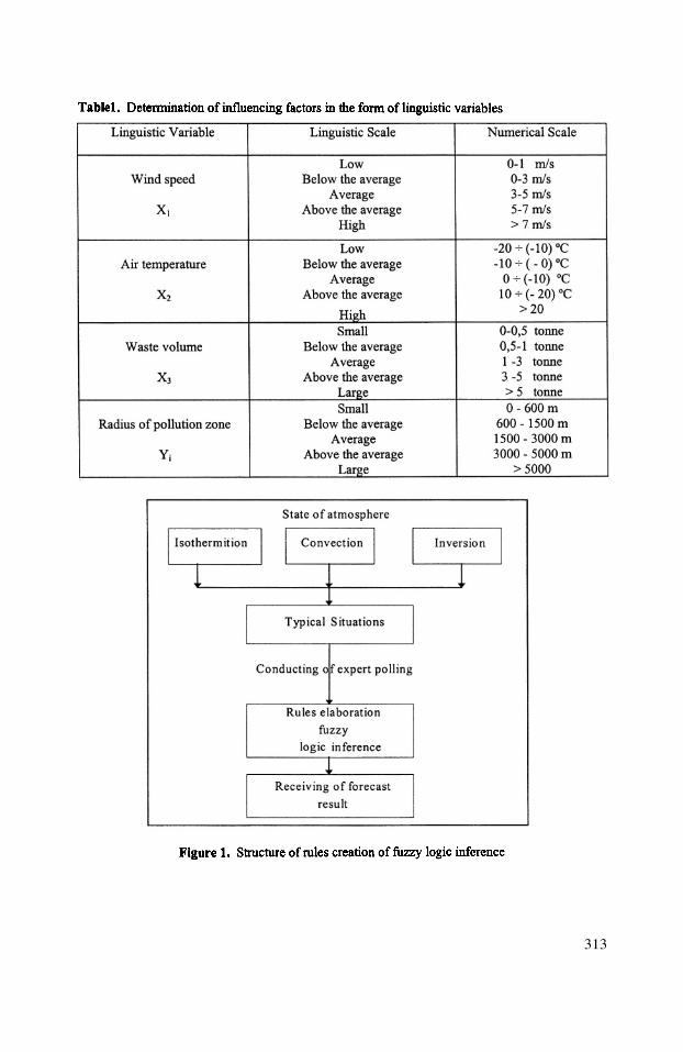
313
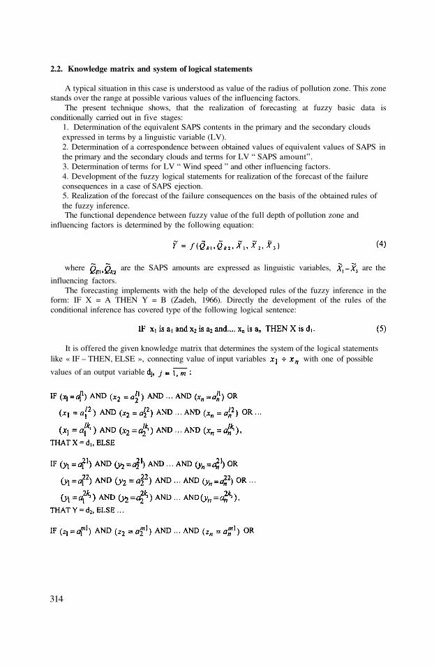
2.2. Knowledge matrix and system of logical statements
A typical situation in this case is understood as value of the radius of pollution zone. This zonestands over the range at possible various values of the influencing factors.
The present technique shows, that the realization of forecasting at fuzzy basic data isconditionally carried out in five stages:
1. Determination of the equivalent SAPS contents in the primary and the secondary cloudsexpressed in terms by a linguistic variable (LV).2. Determination of a correspondence between obtained values of equivalent values of SAPS inthe primary and the secondary clouds and terms for LV “ SAPS amount”.3. Determination of terms for LV “ Wind speed ” and other influencing factors.4. Development of the fuzzy logical statements for realization of the forecast of the failureconsequences in a case of SAPS ejection.5. Realization of the forecast of the failure consequences on the basis of the obtained rules ofthe fuzzy inference.The functional dependence between fuzzy value of the full depth of pollution zone and
influencing factors is determined by the following equation:
where are the SAPS amounts are expressed as linguistic variables, are the
influencing factors.The forecasting implements with the help of the developed rules of the fuzzy inference in the
form: IF X = A THEN Y = B (Zadeh, 1966). Directly the development of the rules of theconditional inference has covered type of the following logical sentence:
It is offered the given knowledge matrix that determines the system of the logical statementslike « IF – THEN, ELSE », connecting value of input variables with one of possible
values of an output variable
314
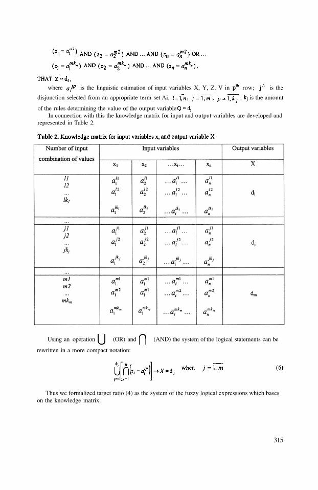
where is the linguistic estimation of input variables X, Y, Z, V in row; is the
disjunction selected from an appropriate term set Ai, is the amount
of the rules determining the value of the output variableIn connection with this the knowledge matrix for input and output variables are developed and
represented in Table 2.
Using an operation (OR) and (AND) the system of the logical statements can be
rewritten in a more compact notation:
Thus we formalized target ratio (4) as the system of the fuzzy logical expressions which baseson the knowledge matrix.
315

3. RESEARCH RESULT
The research of possible depths of pollution zones allows making a conclusion, that it isnecessary to accept inversion from the three possible states of the atmosphere during consequencesof failure at fuzzy initial data. Inversion is considered as a state which lead to maximum depth of apollution zone.
Therefore in case of equal conditions, the solution is accepted proceeding from a condition:
where is the forecast depth or the radius of pollution zone; is the forecast depth of a
pollution zone in case of isothermition; is the forecast depth of a pollution zone in case of
convection; is the forecast depth of a pollution zone in case of inversions.
Thus when forecasting consequences of failure with SAPS ejection, in case of absence ofaccurate initial data the rule of inference are applied to a state of atmosphere - inversion. It isproved from the point of view of minimization of the risk of the population losses in a pollutionzone. Nevertheless, economic costs will be always maximum and not always justified. Forexample, in daytime the atmospheric state can be only isothermition or convection. Therefore indaytime the forecast of consequences is expedient to conduct taking into account isothermition, asstates of atmosphere leading to the large radius of pollution. Proceeding from it, the determinationof depth of a pollution zone at fuzzy initial data is offered to present as:
where ( - for night, - for day)
As a result of researches the values of radius of pollution zone during isothermition areobtained and are represented in Table 3.
316
4. CONCLUSION
Divergence of calculation results of radius and area of polluted zone during certain period oftime do not exceed:
On the accurate input data for radius of polluted zone - 3 %; for pollution area - 20 %.On the recommended traditional technique with use of maximum volume of an ejection,inversion and wind speed (1 m\s) for radius of polluted zone - to 10 %; for pollution area -50-150%.On the model use on the expert evaluations basis for radius of polluted zone -4 %; forpollution area 0-30%.
The offered engineering approach allows effectively conducting the first forecast in case ofabsence of the initial data. The advantage of the given technique is that its use allows savingsignificant costs at the expense of more actual forecasting.
5. REFERENCES
Filinyuk N., Molchanov P., Dudatiev A., 1998, A Comprehensive Evaluation of Industrial Vehicle Safety , AVCS ’ 98:International Conference on Advances in Vehicle Control and Safety to Publication Chair HEUDIASYC/UTS-Compiegne, France, pp.105-107.
Rotshtayn A.P., 1999, Intellectual Technologies of Identification: Fuzzy Sets, Genetic Algorithm, Universum-Vinnitsa,Vinnytsia, P 320.
Ukraine Stuff of Civil Defense, 1999, Technique of forecasting of scopes of infection toxic substances for failures onchemical dangerous objects and transport, Kiev, p. 42.
Zadeh L.A., 1966, Fuzzy Sets, Inf.Control, vol. 18, pp. 338-353.
317

DISCUSSION
M. KAASIK
Y. PODOBNA
A. HANSEN
Y. PODOBNA
Did you use the degrees centigrade (°C) to calibrate the linguistictemperature scale ? If yes, then the scale seems to fit to arcticregions.
Yes, we used the (°C) for the calculation and appropriatedetermination of this influencing factor (air temperature) as alinguistic variable and numerical scale.This was shown for typical example (chemically dangerous object,Vinnytsia).
Do you plan to extend your estimation methodology to includepollutant concentrations as well as pollutant zone ?
We will plan to extend the evaluation of concentrations. (as soon aspossible). But now we have a work about assessment of primaryforecast, and primary calculation for cases when the exact initial dataare absent.
318

INITIAL APPLICATION OF THE ADAPTIVEGRID AIR QUALITY MODEL
M. Talat Odman, Maudood Khan, Ravi Srivastava, and D. Scott McRae*
1. INTRODUCTION
Grid size (or resolution), when inadequate, can be an important source of uncertaintyfor air quality model (AQM) simulations. Coarse grids used because of computationallimitations may artificially diffuse the emissions, leading to significant errors in theconcentrations of pollutant species, especially those that are formed via non-linearchemical reactions. Further, coarse grids may result in large numerical errors. To addressthis issue, multi-scale modeling and grid nesting techniques have been developed(Odman and Russell, 1991; Odman et al., 1997). These techniques use finer grids in areasthat are presumed to be of interest (e.g., cities) and coarser grids elsewhere (e.g., rurallocations). Limitations include loss in accuracy due to grid interface problems andinability to adjust to dynamic changes in resolution requirements. Adaptive grids are notsubject to such limitations and do not require a priori knowledge of where to place finergrids. Using grid clustering or grid enrichment techniques, they automatically allocatefine resolution to areas of interest. They are thus able to capture the physical andchemical processes that occur in the atmosphere much more efficiently than their fixedgrid counterparts.
The adaptive grid methodology used here is based on the Dynamic SolutionAdaptive Grid Algorithm (DSAGA) of Benson and McRae (1991). It employs astructured grid with a constant number of grid nodes. The modeling domain is partitionedinto N×M quadrilateral grid cells. The grid nodes are re-positioned in a twodimensional space throughout the simulation according to a weight function whichrepresents the resolution requirements. The area of the grid cells change due to grid nodemovements but the connectivity of the grid nodes remains the same. Further, since thenumber of grid nodes is fixed, refinement of grid scales in some regions is accompaniedby coarsening in other regions where the weight function has smaller values. This resultsin optimal use of computational resources and yields a continuous multiscale grid where
Talat Odman, Georgia Institute of Technology, Atlanta, Georgia, 30332-0512, [email protected],Telephone: 770-754-4971, Fax: 770-754-8266. Maudood Khan, Georgia Institute of Technology, Atlanta,Georgia, 30332-0512. Ravi Srivastava, U.S. Environmental Protection Agency, Research Triangle Park,North Carolina, 27711. Scott McRae, North Carolina State University, Raleigh, North Carolina, 27695-7910.
Air Pollution Modeling and Its Application XV, Edited byBorrego and Schayes, Kluwer Academic/Plenum Publishers, New York, 2002 319
*
the scales change gradually. Unlike nested grids there are no grid interfaces therefore,numerical problems related to the discontinuity of grid scales are avoided.
The adaptive grid algorithm was applied to problems with increasing complexity andrelevance to air quality modeling. Starting with pure advection tests (Srivastava et al.,2000), it was applied to reactive flows (Srivastava et al., 2001 a) and to the simulation of apower-plant plume (Srivastava et al., 2001b). In all these applications, the adaptive gridsolution was more accurate than a fixed, uniform grid solution obtained by using thesame number of grid nodes. To achieve the same level of accuracy with the fixed uniformgrid required significantly more computational resources than the adaptive grid solution.In this paper, we describe how the adaptive grid algorithm was implemented in an urban-to-regional scale AQM. After a brief discussion of model components, we reportpreliminary results from the first application of the adaptive grid AQM.
2. METHODOLOGY
An adaptive grid AQM simulation has two fundamental steps: a grid adaptation step,that is responsible for repositioning of grid nodes according to the grid resolutionrequirements, and a solution step, that simulates the physical and chemical processes thatoccur in the atmosphere. The solution (i.e., concentration fields) remains unchangedduring the adaptation step and the weight function clusters the grid nodes in regionswhere finer resolution grids are required. In preparation for the solution step, the fields ofmeteorological inputs and emissions must be mapped onto the new grid locations. Thistask is also considered part of the adaptation step and is undertaken by efficient searchand intersection algorithms. During the solution step, the grid nodes remain fixed whilethe solution is advanced in time. Ideally, the adaptation step should be repeated after eachsolution step owing to the change in resolution requirements. However, since themapping of meteorological and emissions data is computationally expensive, we havechosen to apply the adaptation step less frequently. Whereas, the solution is advanced intime by one hour in several time steps, the adaptation step is performed once every hour.In order to ensure numerical stability, we require that the Courant number be smaller thanunity as we determine the time step of the solution. The rest of this section consists of amore detailed description of the adaptation and solution steps.
2.1. Adaptation Step
The key to adaptation is a weight function that determines where grid nodes need tobe clustered for a more accurate solution. Such a weight function, w, can be built from alinear combination of the errors in the concentrations of various chemical species:
where the Laplacian, represents the error in the computed value of the
concentration of species n. The chemical mechanisms used in AQMs usually have a largenumber of species. Due to non-homogeneous distribution of emissions and disparateresidence times, each species may have very different resolution requirements.
320
Determining such that pollutant concentrations (e.g., ozone) can be estimated most
accurately is a current research topic. Here, all are set to zero, except the one for NO.Further, the grid adaptation is restricted to the horizontal plane and the same gridstructure, which is determined by the surface layer NO concentrations, is used for allvertical layers. This combined with the requirement that the Courant number should beless than unity may result in very small solution time steps because of high wind speedsaloft. Adaptation in the vertical direction is possible but significantly more complicated.
Repositioning of the grid nodes is accomplished by using the weight function. The
new position of the grid node i, is calculated as,
where are the original positions of the centroids of the four cells that
share the grid node i and are the associated weight function values.
Once the grid nodes are repositioned, cell-averaged species concentrations must berecomputed for the adapted grid cells. Holding the concentration field fixed and movingthe grid is numerically equivalent to simulating the advection process on a fixed grid.Therefore, we use a high-order accurate and monotonic advection scheme known as thepiecewise parabolic method (Collela and Woodward, 1984) to interpolate concentrationsfrom the old to the new grid locations.
The calculation of the weight function, the movement of the grid nodes and theinterpolation of species concentration from the old to the new grid locations are threedistinct tasks of an iterative process. The process continues until the maximum grid nodemovement is less than a preset tolerance. A very small tolerance may lead to a largenumber of iterations. On the other hand, a large tolerance may not assure adequateresolution of the solution field. Currently, we stop iterating when, for any grid node, themovement is less than 5% of the minimum distance between the node in question and thefour nodes that it is connected to.
After the grid nodes are repositioned, emissions and meteorological data must beprocessed to generate the necessary inputs for the solution step. Note that, unlike thepractice with fixed grid AQMs, this processing could not be performed prior to thesimulation because there is no a priori knowledge of where the nodes would be located atany given time. In case of meteorological data, an ideal solution would be to run ameteorological model (MM), which can operate on the same adaptive grid, in parallel,with the AQM. This would assure dynamic consistency of meteorological inputs but sucha MM is currently nonexistent. Therefore, hourly meteorological data is obtained from ahigh-resolution, fixed grid MM simulation and interpolated onto the adaptive grid. Formass conservation, as a minimum requirement, the vertical wind components arereadjusted later during the solution step as described in Odman and Russell (2000).
The processing of emission data is computationally an expensive task that requiresidentification of various emission sources falling into the adapted grid cells. Here, wetreat all emissions in two categories: point and area source emissions. For simplicity, themobile sources have been included in the area-source category, but treating them as linesources would yield better resolution. For the point sources, the grid cell containing the
321
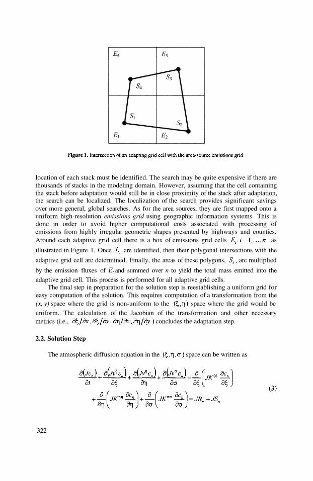
location of each stack must be identified. The search may be quite expensive if there arethousands of stacks in the modeling domain. However, assuming that the cell containingthe stack before adaptation would still be in close proximity of the stack after adaptation,the search can be localized. The localization of the search provides significant savingsover more general, global searches. As for the area sources, they are first mapped onto auniform high-resolution emissions grid using geographic information systems. This isdone in order to avoid higher computational costs associated with processing ofemissions from highly irregular geometric shapes presented by highways and counties.Around each adaptive grid cell there is a box of emissions grid cells as
illustrated in Figure 1. Once are identified, then their polygonal intersections with the
adaptive grid cell are determined. Finally, the areas of these polygons, are multiplied
by the emission fluxes of and summed over n to yield the total mass emitted into theadaptive grid cell. This process is performed for all adaptive grid cells.
The final step in preparation for the solution step is reestablishing a uniform grid foreasy computation of the solution. This requires computation of a transformation from the(x, y) space where the grid is non-uniform to the space where the grid would beuniform. The calculation of the Jacobian of the transformation and other necessarymetrics (i.e., concludes the adaptation step.
2.2. Solution Step
The atmospheric diffusion equation in the space can be written as
322
where and are the concentration, chemical reaction and emission terms ofspecies n, respectively, and is a terrain-following vertical coordinate. J is the Jacobianof the coordinate transformation:
where m is the scale factor of a conformal map projection in the horizontal. The
components of the wind vector in and directions are and
where U and V are real horizontal wind velocities rotated in the map’s coordinatedirections. The turbulent diffusivity tensor is assumed to be diagonal and its elements are
and . The last element can be expressed in terms of the verticaldiffusivity as
The expressions for the wind component in the direction, as well as
and are omitted here due to space limitations. Since the grid is uniform in thespace, solution algorithms can be taken directly from existing AQMs. We use
those described by Odman and Ingram (1996).
3. MODEL VERIFICATION
The adaptive grid AQM is being verified by simulating ozone air quality in theTennessee Valley region for the July 7-17, 1995 period. Meteorological data from a4 × 4 km resolution simulation with the Regional Atmospheric Modeling System(RAMS) is being used. The emissions inputs for the region were developed from theSouthern Appalachian Mountains Initiative (SAMI) inventory. There are over 9000 pointsources in this domain including some of the largest power plants in the U.S.A. The areasources were mapped onto a 4 × 4 km emissions grid. The AQM grid consists of 112 by64 cells, initially at 8 × 8 km resolution. In the vertical, there are 20 unequally spacedlayers extending from the surface to 5340 m. Starting with 32 m, the thickness of eachlayer increases with altitude.
Figure 2 shows the grid at 7:00 EST on July 7. Since the adaptation step is performedonce an hour, the grid shown will not change until 8:00 EST. Note that the grid size
323
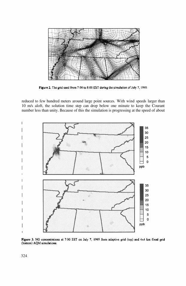
reduced to few hundred meters around large point sources. With wind speeds larger than10 m/s aloft, the solution time step can drop below one minute to keep the Courantnumber less than unity. Because of this the simulation is progressing at the speed of about
324
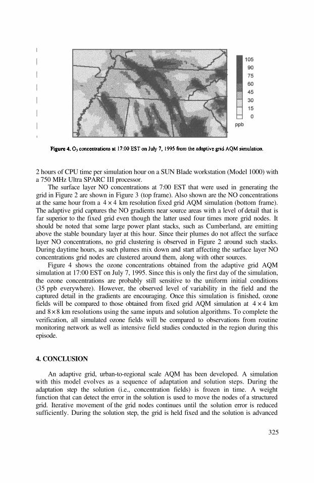
2 hours of CPU time per simulation hour on a SUN Blade workstation (Model 1000) witha 750 MHz Ultra SPARC III processor.
The surface layer NO concentrations at 7:00 EST that were used in generating thegrid in Figure 2 are shown in Figure 3 (top frame). Also shown are the NO concentrationsat the same hour from a 4 × 4 km resolution fixed grid AQM simulation (bottom frame).The adaptive grid captures the NO gradients near source areas with a level of detail that isfar superior to the fixed grid even though the latter used four times more grid nodes. Itshould be noted that some large power plant stacks, such as Cumberland, are emittingabove the stable boundary layer at this hour. Since their plumes do not affect the surfacelayer NO concentrations, no grid clustering is observed in Figure 2 around such stacks.During daytime hours, as such plumes mix down and start affecting the surface layer NOconcentrations grid nodes are clustered around them, along with other sources.
Figure 4 shows the ozone concentrations obtained from the adaptive grid AQMsimulation at 17:00 EST on July 7, 1995. Since this is only the first day of the simulation,the ozone concentrations are probably still sensitive to the uniform initial conditions(35 ppb everywhere). However, the observed level of variability in the field and thecaptured detail in the gradients are encouraging. Once this simulation is finished, ozonefields will be compared to those obtained from fixed grid AQM simulation at 4 × 4 kmand 8 × 8 km resolutions using the same inputs and solution algorithms. To complete theverification, all simulated ozone fields will be compared to observations from routinemonitoring network as well as intensive field studies conducted in the region during thisepisode.
4. CONCLUSION
An adaptive grid, urban-to-regional scale AQM has been developed. A simulationwith this model evolves as a sequence of adaptation and solution steps. During theadaptation step the solution (i.e., concentration fields) is frozen in time. A weightfunction that can detect the error in the solution is used to move the nodes of a structuredgrid. Iterative movement of the grid nodes continues until the solution error is reducedsufficiently. During the solution step, the grid is held fixed and the solution is advanced
325

in time. However, before this can be done, the meteorological and emissions inputs mustbe mapped onto the adapted grid. For meteorological inputs, data are interpolated from avery high-resolution mesoscale model simulation. For emissions, efficient search andintersection algorithms were developed to assure proper allocation of point and areasources to the cells of the adapted grid. Using coordinate transformations, the non-uniform grid can be mapped into a space where it becomes uniform. The atmosphericdiffusion equation in this new space has been derived. Since the form of the equation isvery similar to forms in existing AQMs and the grid is uniform, numerical algorithmsdeveloped for fixed uniform grid AQMs can be used to advance the solution.
To verify the model, the July 7-17, 1995 ozone episode in the Tennessee Valley isbeing simulated. So far, the grid is adapting to dynamic changes in the NO fields asexpected. Nodes are clustered around major emission sources with grid resolutionsaround 200 m. The NO and fields show gradients with a level of detail that is likelyunprecedented for a regional simulation of this scale. However, the simulation isprogressing slowly due to very short solution time steps. This will probably necessitatechanges in solution algorithms such as using an implicit advection scheme that is notsubject to the Courant stability limit. Adaptation criteria are also being developed thatwould consider the errors not only in NO but in other species as well, especially thoseinvolved in important ozone formation reactions.
5. ACKNOWLEDGEMENTS
This research is supported by the U.S. Environmental Protection Agency under GrantAgreement No. R 827028-01-0. We thank Dr. Steve Mueller of the Tennessee ValleyAuthority for providing the meteorological data.
6. REFERENCES
Benson, R. A., and McRae, D. S., 1991, A Solution adaptive mesh algorithm for dynamic/static refinement oftwo and three-dimensional grids, in: Proceedings of the Third International Conference on NumericalGrid Generation in Computational Field Simulations, Barcelona, Spain, p. 185.
Collela, P., and Woodward, P. R., 1984, The piecewise parabolic method (PPM) for gas-dynamical simulations,J. Comput. Phys. 54:174.
Odman, M. T., and Russell, A.G., 1991, A multiscale finite element pollutant transport scheme for urban andregional modeling, Atmos. Environ. 25A: 2385.
Odman, M. T., and Ingram, C., 1996, Multiscale Air Quality Simulation Platform (MAQSIP): Source CodeDocumentation and Validation, MCNC Technical Report ENV-96TR002, Research Triangle Park, NorthCarolina, pp. 11-32.
Odman, M. T., Mathur, R., Alapaty, K., Srivastava, R. K., McRae, D. S., and Yamartino, R. J., 1997, Nestedand adaptive grids for multiscale air quality modeling, in: Next Generation Environmental Models andComputational Methods, G. Delic, and M. F. Wheeler, eds., SIAM, Philadelphia, pp. 59-68.
Odman, M. T, Russell, A. G., 2000. Mass conservative coupling of non-hydrostatic meteorological models withair quality models, in: Air Pollution Modeling and its Application XIII, S.-E.Gryning, and E. Batchvarova,eds., Kluwer Academic/Plenum Publishers, New York, pp. 651-660.
Srivastava, R. K., McRae, D. S., and Odman, M. T., 2000, An adaptive grid algorithm for air quality modeling;J. Comput. Phys. 165: 437.
Srivastava, R. K., McRae, D. S., and Odman, M. T., 2001(a), Simulation of a reacting pollutant puff using anadaptive grid algorithm, J. Geophys. Res., in press.
Srivastava, R. K., McRae, D. S., Odman, M. T., 2001(b), Simulation of dispersion of a power plant plume usingan adaptive grid algorithm, Atmos. Environ., in press.
326

DISCUSSION
C. MENSINK
M. KHAN
O. HELLMUTH
M. KHAN
A. HANSEN
M. KHAN
Your adaptive grid method is applied in two dimensions, using aLaplacian weighting function. Assuming that vertical diffusionprocesses are more important than horizontal diffusion processes itmight be interesting to use grid refinement in the vertical direction.Do you think it is possible to extend the method to 3 dimensions ?
Although it would be possible to perform grid adaptions in a 3-dimensional space, the additional computational costs are likely tobe high and improvement in results might not to significant enoughto justify these costs.
The scale dependency of the physical parameterizations becomesmore important in adaptive grid air quality models compared tomodels using a static grid. This might be true especially for thedesign of the eddy diffusivity. How you are going to deal with that ?(maybe the concept of cut-off-wave length (grid size dependent) inconnection with the evaluation of empirical or synthetical turbulencespectra to determine the eddy diffusivity might be worth to beconsidered). It would be nice to see, that your grid approach givearguments for turbulence modellers to deal further on with scale-dependent turbulence parameterizations.
We are aware of these issues and plan to look at otherparameterization techniques that might be more appropriate foradaptive grid air quality models.
Is your adaptive grid methodology mass conservative ?What is the magnitude of numerical diffusion associated with yourscheme ?
We are conserving mass and using the same numerical algorithms asare used by the static grid to advance the solution in time.
327

C.FUNG
M. KHAN
It seems that the adaptive grid also balances the chemistry solverload. Has the run time increased or decreased ?
Run time has increased but the improvement in air quality modelingresults more than justifies these additional computational costs.
328
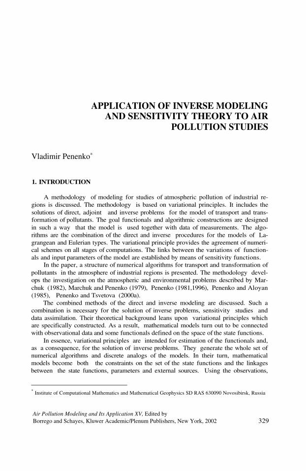
APPLICATION OF INVERSE MODELINGAND SENSITIVITY THEORY TO AIR
POLLUTION STUDIES
Vladimir Penenko*
A methodology of modeling for studies of atmospheric pollution of industrial re-gions is discussed. The methodology is based on variational principles. It includes thesolutions of direct, adjoint and inverse problems for the model of transport and trans-formation of pollutants. The goal functionals and algorithmic constructions are designedin such a way that the model is used together with data of measurements. The algo-rithms are the combination of the direct and inverse procedures for the models of La-grangean and Eulerian types. The variational principle provides the agreement of numeri-cal schemes on all stages of computations. The links between the variations of function-als and input parameters of the model are established by means of sensitivity functions.
In the paper, a structure of numerical algorithms for transport and transformation ofpollutants in the atmosphere of industrial regions is presented. The methodology devel-ops the investigation on the atmospheric and environmental problems described by Mar-chuk (1982), Marchuk and Penenko (1979), Penenko (1981,1996), Penenko and Aloyan(1985), Penenko and Tsvetova (2000a).
The combined methods of the direct and inverse modeling are discussed. Such acombination is necessary for the solution of inverse problems, sensitivity studies anddata assimilation. Their theoretical background leans upon variational principles whichare specifically constructed. As a result, mathematical models turn out to be connectedwith observational data and some functionals defined on the space of the state functions.
In essence, variational principles are intended for estimation of the functionals and,as a consequence, for the solution of inverse problems. They generate the whole set ofnumerical algorithms and discrete analogs of the models. In their turn, mathematicalmodels become both the constraints on the set of the state functions and the linkagesbetween the state functions, parameters and external sources. Using the observations,
* Institute of Computational Mathematics and Mathematical Geophysics SD RAS 630090 Novosibirsk, Russia
Air Pollution Modeling and Its Application XV, Edited byBorrego and Schayes, Kluwer Academic/Plenum Publishers, New York, 2002
1. INTRODUCTION
329

mathematical models are applied for estimation of initial fields, for reconstruction ofthe time and space structure of the state functions and for more precise definition ofmodel parameters. The proposed algorithms allow the estimation of model quality anddata assimilation to be made simultaneously. To this purpose the optimization methodscombined with the methods of model sensitivity evaluation are used. Adjoint problemsplay an essential role in the realization of this approach.
The basic elements of four types should be defined to represent the methodology(Penenko, 1996). They are:
mathematical models of investigated processes,mathematical “models of observations” and the functions of environment quality,set of functionals on the space of the state functions,criteria for the model quality , design of observation and management planning.
The term “ model of observations” describes the transformation of the state function tothe observed process characteristics. Observations can be of contact, indirect and remotetypes. They determine the structure of the corresponding models.
The following notations are used here: is a state vector, is a parameter vector, B is
a diagonal matrix, some diagonal elements of which can be zero, is a non-linear
space operator , is a function of sources, D is a domain of spatial
variables is the time interval, is the space of state functions satisfying
the boundary conditions, is the range of admissible parameter values. For the
considered class of problems the operator is defined by the hydrodynamicequations of the “atmosphere-water-earth” system, transport and transformation ofpollutants, and by the relations at the interface boundaries. It includes all the termsof equations except the time derivatives.
The initial conditions at t = 0 and the model parameters can be written in the form
2. MODELS OF THE PROCESSES
The advantage of operator notations is used to describe a general structure of algo-rithms . The model is written in the form
Here, and are the given a priori estimates of the initial fields and the pa-
rameters’ vector The boundary conditions for the closure of the model are the con-sequences of the physical content of the problem under investigation. To include obser-vational data into the model processing, it is necessary to formulate the functionalrelationship between the measurements themselves and the state functions. Let thisrelation take the form
330
Here is the set of observed values; is the set of measurement models. The
values of are defined on the set of points The terms
and in (1)-(3) take into account the errors and uncertainties of the mod-els, initial state, parameters and measurement models respectively. If the model andinput data are exact, then the error terms should be omitted.
3. VARIATIONAL DESCRIPTION OF THE MODEL
To construct the direct and inverse modeling algorithms, it is necessary to haveboth the differential and variational formulations of the models. Let us give the varia-tional form of the model (1)-(3) by means of the integral identity (Penenko, 1996)
Here is an arbitrary sufficiently smooth co-state function, is the space of
sufficiently smooth functions defined in that is conjugated to The functional
in (4) is formed so that all the equations of model (1), initial and boundary
conditions, conditions at the interface boundaries and external sources are includedin it simultaneously. The form of the functional and inner scalar product in (4) are gener-ated from the form of the total energy balance equation for model (1).
For example, the identity (4) for the model of transport and transformation of pollut-ants in the atmosphere has the form
where are the state function, adjoint or
co-state function and parameter vector, are the concentrations of pollutants, n is thenumber of substances, is the transport operator, H is pollutants’ transformation op-erator L is the boundary conditions operator, and are the boundaries of the do-
mains D and (Penenko and Aloyan, 1985, Penenko, Skubnevskaya et al., 1997 ,
Penenko and Tsvetova, 1999a).
331

Here are some functions of of the given form and are non-negative
weight functions; are the corresponding Radon’s or Dirac’s measures
(Schwartz, 1967). In particular, the functions can have a finite support in A
low limit case occurs when one point acts as a support. Then the Dirac delta-function isthe weight function for this case. In the finite dimensional formulation, it is
replaced by the Kronecker delta-function.The functionals of five main types should be outlined: functionals of generalized de-
scription of the system behavior; quality functionals which evaluate deviations betweenmeasured and calculated values, measurement functional; restriction functionals, objec-tive or cost functionals for control and design. The restriction functionals are introducedto take into account both the local and global constrains to the atmospheric quality in theproblems of ecological management and design.
Let us use the ideas of optimization theory and variational technique for the state-ment of inverse problems and for the construction of methods for their solution. In thiscase, all approximations are defined by the structure of the quality functional and by theway of its minimization on the set of values of the state functions, parameters and errorsof the discrete formulation of the model. The basic functional is formulated so that all theavailable data, errors of the numerical model and input parameters are taken into account(Penenko, 1996):
332
4. FUNCTIONALS AS GENERALIZED CHARACTERISTICS OF THEPROCESSES
From the point of view of computational technology, the methods of inverse model-ing are more suited to the work with global (integral) characteristics of the models andprocesses than to the work with the local ones. That is why we determine the set of suchobjects in the form
5. GENERAL FUNCTIONAL FOR INVERSE MODELING ALGORITHMS
where are weight matrices. Here the first term is given by (6), the second termtakes into account the model errors, the third term describes errors in the initial data, thefourth term is responsible for the errors of the parameters, the fifth term is evaluation ofmeasured data errors , and the last one is a numerical model of the processes in a varia-tional form, indexes h and T denote discrete analog and operation of transposition ofcorresponding objects .To continue, a minimization functional problems with respect to
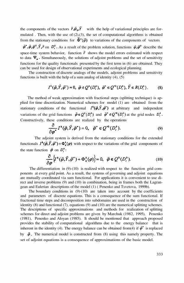
The differentiation in (9)-(10) is realized with respect to the function grid com-ponents at every grid point. As a result, the systems of governing and adjoint equationsare mutually coordinated via sum functional. For applications it is convenient to use di-rect and inverse problems (9) and (10) in combination, being in frames both the Lagran-gean and Eulerian descriptions of the model (1) ( Penenko and Tsvetova, 1999b).
The boundary conditions in (9)-(10) are taken into account by the coefficientsand parameters of discrete equations. This is a consequence of the sum functional. Iffractional time steps and decomposition into subdomains are used in the construction ofidentity (8) and functional (7), equations (9) and (10) are the numerical splitting schemes.The descriptions of specific approximations and methods for realization of splittingschemes for direct and adjoint problems are given by Marchuk (1982, 1995), Penenko(1981), Penenko and Aloyan (1985). It should be mentioned that approach proposedprovides the stability of computational algorithms due to the energy balance that isinherent in the identity (4). The energy balance can be obtained from(4) if is replaced
by The numerical model is constructed from (8) using this namely property. The
set of adjoint equations is a consequence of approximations of the basic model.
333
the components of the vectors with the help of variational principles are for-
mulated . Then, with the use of (2),(3), the set of computational algorithms is obtained
from the stationary conditions for to variations of the components of vectors
on As a result of the problem solution, functions describe the
space-time system behavior, function shows the model errors estimated with respectto data Simultaneously, the solutions of adjoint problems and the set of sensitivity
functions for the quality functionals presented by the first term in (6) are obtained. Theycan be used for design of observational experiments and ecological planning.
The construction of discrete analogs of the models, adjoint problems and sensitivityfunctions is built with the help of a sum analog of identity (4), (5)
The method of weak approximation with fractional steps (splitting technique) is ap-plied for time discretization. Numerical schemes for model (1) are obtained from the
stationary conditions of the functional at arbitrary and independent
variations of the grid functions and at the grid nodes
Constructively, these conditions are realized by the operations
The adjoint system is derived from the stationary conditions for the extended
functionals with respect to the variations of the grid components of
the state function on

334
6. ALGORITHMS FOR SENSITIVITY STUDIES
The analysis of the model sensitivity to the variations of input parameters is an es-sential step in the solution of the numerical simulation problems. Especially, this is nec-essary to be done when studying the real physical system behavior with the help of nu-merical models. In this case, sensitivity functions play a substantial role .If the model isconsidered together with observational data, the sensitivity functions make it possibleto realize interrelations between observations and models. Algorithmically, the sen-sitivity analysis gives numerical values of the gradients of the functional (6) with respectto model parameters that are required for realizing optimization methods. By the way,we pose the problem of data assimilation in the models as a problem of optimization.
The construction of the main sensitivity relation is made according to algorithm
where is the variation of evaluated functional, are the solution of the (10)
and (11) with the unperturbed values of is real parameter, are
the variations ofThe calculation of the sensitivity function is made by the formula
The sensitivity relations for the model of transport and transformation of pollutants(5) have the form
Here symbol denotes variations of corresponding elements. The variations of theoperators in (13) are calculated with the use of the variation of their parameters.
Multipliers at variations are the sensitivity functions of to the correspondingvariations. The definition of sensitivity functions allows the equations of feedback be-tween parameters and functionals (6) to be introduced into the model set:

where are the proportional coefficients that are calculated during the functional estima-
tion procedure. The methods of direct modeling are based on the solution of the problem(9). The field of application of inverse modeling is wider than that of direct one. In ourcase the structure of inverse modeling algorithms are defined by the relations (10)-(14).
Depending on the statements of the problems and the purposes of investigation, thedifferent applications of the modeling technology can be realized. Here we list the mosttypical cases oriented to the problems of forecasting, monitoring and ecological design.In addition to the problems that are usually solved in the frameworks of direct modelingprocedure, the following problems are connected with the combination of the direct andinverse modeling: calculation of sensitivity functions and variations of functionals; in-verse problems for diagnosis and identification of parameters and sources of the model;data assimilation; comparison of the models and fitting the models of different scales;zoning the domains in accordance with the man-induced load levels; ecological designand risk evaluation; detection of the sources of pollution; atmospheric quality control;estimation of the informative content of monitoring systems; planning observations. Al-gorithms to the solution of the above listed problems are obtained as modifications of thegeneral inverse modeling algorithm. The different aspects of methodology presentedare described in the papers of the author and co-authors. The calculations are made onthe base of the global model of pollutant transport. The atmospheric circulation for sce-narios are reconstructed from Reanalysis data (Kalnay et al., 1996) in assimilation modewith the help of the system described by Penenko and Tsvetova (1999c). The “direct”problems of the “source-receptor” type and inverse problems of the “receptor-source”type are of great interest for the environmental quality studies. They allow ecologicallydangerous regions for surroundings to be revealed and high risk vulnerability territoriesto be detected. Some examples of such problems are given by Penenko, Aloyan et al.,(1989), Penenko and Tsvetova ( 1999b, 2000a, 2000b), Penenko (2001).
Penenko and Tsvetova (1999b) study the scales of interconnections in the climaticsystem. The two scenarios agreed with respect to the time interval are considered. Thefirst one is the “direct” scenario on transport of pollutants while the Chernobyl accident.The second one is the inverse modeling scenario on estimation of danger for Lake Baikalto be polluted within the above mentioned time interval.
The inverse scenarios in Lagrangean and Eulerian statements are presented byPenenko and Tsvetova ( 2000a). The problem on identification of the sources thatspread the bio-aerosols in the Western Siberian region is considered. Besides, estimationof the sources observability areas is made for the measuring site. The scenario on esti-mation of the domains in the Northern Hemisphere that could be polluted as the conse-quence of the release from aggregated sources in Central Europe is described byPenenko and Tsvetova (2000b). The technique for estimation of ecological risk is doneby Penenko (2001). Japan, and the Russian Far East are revealed as examples of thedomains of high ecological risk.
335
7. APPLIED PROBLEMS

The problems under discussion are very complicated. In this connection some waysof increasing the efficiency of the algorithms should be mentioned. The general func-tional (7) is constructed so that all the models and functionals are additively includedin it. As a consequence of the fact, we are able to generate multilevel parallel schemesby means of variational principles. This is one more evidence that the proposed approachappears to have considerable promise.
The work is supported by the RFBR under the Grants 99-07-90422, 00-15-98543,01-05-65313, the Russian Ministry of Industry and Science (0201.06.269/349), andEuropean Commission (ICA2-CT-2000-10024).
Kalnay, E., Kanamitsu, M., Kistler, R., et al.,1996, The NCEP/NCAR 40-year reanalysis project. Bull. Amer.Meteorol. Soc. 77, 437-471.
Marchuk, G. I.,1982,Mathematical Modeling in the Environmental Problem, [ in Russian], Nauka, Moscow,320 p.
Marchuk, G. I. ,1995, Adjoint Equations and Analysis of Complex Systems Kluwer Academic Publication.Marchuk, G. I., Penenko, V.V.,1979, Application of optimization methods to the problem of mathematical
simulation of atmospheric processes and environment. Proc. IFIP-TC7 Conf., N.Y. Springer., 240-252.Penenko, V.V.,1981, Methods of Numerical Modeling of the Atmospheric Processes, [ in Russian], Lenin-
grad, Gidrometeoizdat, p. 352.Penenko, V.V., 1996, Some aspects of mathematical modeling using the models together with observational
data. Bull. Nov. Comp. Center, Num. model. in atmosph., N 4, 31-52.Penenko, V.V., 2001, Revealing the areas of high ecological vulnerability: the concept and approach to reali-
zation. Atmos. Oceanic. Opt., 14, 596-601.Penenko, V.V., Aloyan, A.E., 1985, Models and Methods for Environment Protection Problems, [ in Russian],
Nauka, Novosibirsk, 256 p.Penenko, V.V., Aloyan, A.E., Tsvetova, E.A. et al.,1989, Numerical estimation of anthropogenic loads on Lake
Baikal , Soviet Meteor. and Hydrol. No 7, 76-84.Penenko, V.V., Skubnevskaya.G.I., Tsvetova, E.A. et at., 1997, Numerical simulation of chemical kinetics and
transfer of pollutants in the atmosphere of industrial regions. Chemistry for sustainable development, 5,505-510.
Penenko, V.V., Tsvetova, E.A., 1999a, Mathematical models for the study of interactions in the system LakeBaikal-atmosphere of the region. J. of Applied Mechanics and Technical Physics, 40, 308-316.
Penenko, V.V., Tsvetova,E.A., 1999b, Modeling of pollutant transport in direct and inverse problems of cli-matic-ecological monitoring and prediction, Atmos. Oceanic Opt., 12, 462-467.
Penenko, V.V., Tsvetova, E.A., 2000a, Some aspects of solving interrelated problems of ecology and climate.J. of Applied Mechanics and Technical Physics, 41, 907-914.
Penenko, V.V., Tsvetova, E.A., 1999c, Preparation of data for ecological studies with the use of Reanalysis.Atmos. Oceanic Opt., 12, 447-449.
Penenko, V.V., Tsvetova, E.A., 2000b, A scale analysis of anthropogenic impact in the atmosphere. Atmos.Oceanic Opt., 13, 392- 396.
Schwartz, L ., 1967 Analise Matematique, Hermann.
336
8. CONCLUSION
The proposed approach extends the capabilities of the models for diagnosing andpredicting the processes in the climatic system and for planning and evaluating the in-formation quality of observations.
ACKNOWLEDGEMENTS
REFERENCES
SENSITIVITY ANALYSIS OF NESTEDPHOTOCHEMICAL SIMULATIONS
Ioannis A. Kioutsioukis and Andreas N. Skouloudis*
Photochemical models predict species concentrations based on a series of physicalprocesses and data describing the status of the domain like, the boundary conditions andthe emissions. The outcome of recent studies, regarding photochemical formation in largeurban environments demonstrated that among the subtle issues to be fully explored(Peters et al. 1995; Pielke, 1998) is an evaluation of the sensitivity of an atmosphericchemical model due to perturbations. The magnitude of the perturbations should reflectthe inherent inaccuracies in the observed data.
One of the first studies that utilised photochemical models for examining theimportance of boundary conditions in emission control strategies was that of Winner etal. (1995). Specifically, they used the 3D photochemical model CIT (Harley et al., 1993)for the Los Angeles area (250 km x 150 km) in order to construct the isopleths of for64 different scenarios of and VOC emission reductions. The runs of the model wereexecuted in a supercomputer with 64 processors, which allowed them to produce twoisopleth diagrams. In the first, they used clean (future) boundary conditions while in thesecond observed (present) boundary concentrations. Their results indicate that only withclean boundary conditions, the emission reduction scenario can lead to a harmonisationof the maximum concentration of with the existing limits. In the other case, willnever be in line with the desired limits, for all emission reduction scenarios.
In another study, Hanna et al. (1998) studied the sensitivity of UAM-IV for variousuncertainty parameters including the boundary conditions of and VOC. Themodel was executed for the New York domain (230 km x 290 km) and the sensitivitymethod employed was Monte Carlo. Having 109 uncertain parameters, they performedonly 50 runs, where the uncertain parameters were selected randomly. The result of thispreliminary study is that the maximum concentration of is affected mainly by theVOC emissions followed by the boundary concentrations.
* Ioannis A. Kioutsioukis (TP.361) and Andreas N. Skouloudis (TP.280), EuropeanCommission, Joint Research Centre, Environment Institute, Ispra, 21020, Italy.
Air Pollution Modeling and Its Application XV, Edited byBorrego and Schayes, Kluwer Academic/Plenum Publishers, New York, 2002
1 INTRODUCTION
337
A study of the impact of boundary conditions in real time simulations was conductedby Vautard (2000). The author used the results of the simplified synoptic scalephotochemical model CHIMERE (operationally executed for Paris domain:http://callas.ens.fr) for the summer of 1999 and checked diagnostically the effect ofboundary conditions by comparing the forecasted and observed concentrations. ALagrangian back-trajectory model calculates the boundary conditions in CHIMERE whilethe meteorological data used were from ECMWF forecasts (http:/ /www.ecmwf.int) . Theresult of the study is that about 50% of the prognostic error in the forecastedconcentrations is due to bad prediction of the boundary conditions.
In another study, Ziomas et al. (1998) studied the effect of alternative emissionscenarios for the Athens domain, using data from the MEDCAPHOT-TRACE (Ziomas,1998) campaign. The UAM-IV model was utilised in this work and the results indicatethat the strategies should be focusing on VOC emission reductions.
In this work, are presented an outline of the research funded by EuropeanCommission, Directorate General of Research under the grant ENV4-CT97-5080. In thefollowing sections are examined the effects in the modelled concentrations throughvariations of the boundary conditions and of emissions. This study was carried out withthe Tangent Linear Model (TLM) of the 3D Air Quality model CAMx (ComprehensiveAir-Quality Model with eXtensions). The TLM of CAMx is obtained by utilising theautomatic differentiation tool ADIFOR (Automatic Differentiation in FORtran). TheTLM has been extensively used for sensitivity studies in Meteorology (Errico et al.,1993; Vukicevic 1991, 1993).
Whether presented as a table of results from a set of exploratory runs, or formallyencapsulated as a sensitivity coefficient, most parametric sensitivity studies either areequivalent or can be embedded in a problem of estimating derivatives. By differentiatingthe output of a model with respect to its parameters, one can quantify how sensitive orrobust are the predictions of a model, relative to variations of that parameter, as well asgain insight into how to adjust parameters that are poorly known.
Automatic differentiation techniques augment, in a completely mechanical fashion,an existing code such that it also simultaneously and efficiently computes derivatives.The technique (Rall, 1981; Griewank, 1989) rely on the fact that every function, nomatter how complicated, is executed on a computer as a sequence of elementaryoperations, such as addition or multiplication, and elementary functions, such as squareroot or log. By applying the chain rule of differential calculus to each stage in thissequence, one can compute derivatives of a function exactly (Bischof et al., 1992, 1994,1996, 1998), in a completely mechanical fashion and efficient time saving (Horwedel,1992; Hwang et al., 1997; Carmichael et al., 1997).
A large number of packages for automatic differentiation of model codes written invarious programming languages are currently available. These tools mechanicallygenerate from an existing code an augmented code that in addition computes derivatives.For these sensitivity studies, we used the ADIFOR package. The principal merit of usingADIFOR is that, for just one model run, we can assess the sensitivities of all modeloutputs with respect to all input parameters. Other advantages of the method include the
338
2 SENSITIVITY ANALYSIS USING COMPUTATIONAL DIFFERENTIATION

can be interpreted as the sensitivity of to a uniform relative change in the boundaryconcentrations of specie j. On the other hand, the global effect of perturbing a variable isstudied in terms of a control function of the form:
where, is the perturbed concentration and the unperturbed one. The symboldenotes the inner product of matrices A and B. The sensitivity of the control function canbe calculated by the LSC as (global sensitivities):
3 RESULTS AND DISCUSSION
The domains for this sensitivity analysis were three cities with fundamentaldifferences in the topography and the emissions. Namely, Athens (Ziomas, 1998; Ziomaset al., 1998), Milan (Volta et al., 1997; Silibello, 1998) and London (Derwent, 1993).These cities represent a typical subset out of eleven cities studied in the Auto-Oil IIprogram (Skouloudis et al., 2001). Also, the CAMx model (Environ, 1998), which is a
339
superb computational precision, ease of creature, as well as the less computationaldemands.
2.1. Methodology
Consider for example the boundary concentration of the pollutant j. If we perturb itby a factor (Park et al., 2000):
Then, any concentration field that is influenced by the boundary concentration of jimplicitly depends upon Expanding in a Taylor series about the referencesolution and retaining only the first-order term, we obtain an approximation ofthe sensitivity of with respect to
The interpretation of sensitivity information will be performed in two different ways:(a) the effect in the system of perturbing a variable and (b) the effect in a variable ofperturbing another variable. The linear estimation of the change in concentration thatoriginates from a unitary perturbation in variable is evaluated by means of the localsensitivity coefficient (LSC) (Saltelli et al., 2000):

Eulerian photochemical grid model that allows for integrated assessment of gaseous andpaniculate air-pollution over many scales, was selected for the air-quality simulations.This model was utilised in a two-way nested formation with an outer-grid resolution of0.06 degrees and with an inner-grid resolution of 0.02 degrees. The exact position ofthese grids is given in Table 1. The simulation period was an ozone episode lasting forseveral days and included the 98%tile concentration for 1995 (base year for AutoOil-II).
3.1. Sensitivity of the System
Figure 1a shows the time evolution of the control function J, which indicates theeffect of each perturbation (boundary conditions) in the system. It is interesting toobserve that the sensitivity of the system is formed into clusters. The highest sensitivityto the whole system arises from perturbations at the boundary conditions of followedby the perturbations at VOC and This hierarchical sequence was reproduced for allthe cities. This implies that these results have a general character. The relative importanceof perturbations at the boundary conditions of VOC, and CO to the system is 1:0.2: 0.09: 0.04 (at the time of observed maximum
The investigated species are shown in Table 1. Among the many available results(Kioutsioukis, 2001), we will concentrate in the effects to the system and to O3.
Similarly, in Figure 1b is shown the effect of perturbations at “area emissions”. Inthis case also, the results for each city are sorted, but not for pollutants. In other words,the highest overall sensitivities are found in Milan and the lowest in London. Thisfollows in analogy with the ratio of among the cities (maximum in Milan,minimum in London). However, we should not forget that the high values of the controlfunction for perturbations in and VOC are related to the sensitivity of and VOC totheir own conditions (net transport of and VOC inside the domain).
340

341
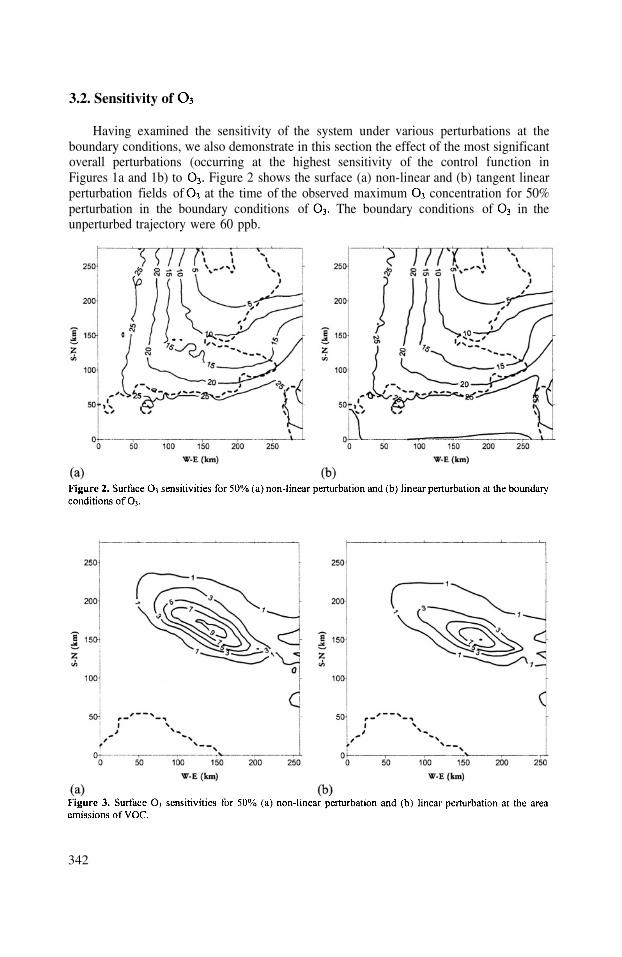
Having examined the sensitivity of the system under various perturbations at theboundary conditions, we also demonstrate in this section the effect of the most significantoverall perturbations (occurring at the highest sensitivity of the control function inFigures 1a and 1b) to Figure 2 shows the surface (a) non-linear and (b) tangent linearperturbation fields of at the time of the observed maximum concentration for 50%perturbation in the boundary conditions of The boundary conditions of in theunperturbed trajectory were 60 ppb.
342
3.2. Sensitivity of
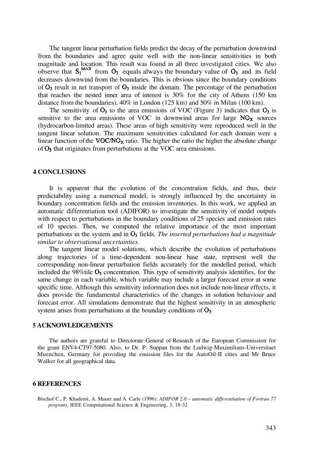
The tangent linear perturbation fields predict the decay of the perturbation downwindfrom the boundaries and agree quite well with the non-linear sensitivities in bothmagnitude and location. This result was found in all three investigated cities. We alsoobserve that from equals always the boundary value of and its fielddecreases downwind from the boundaries. This is obvious since the boundary conditionsof result in net transport of inside the domain. The percentage of the perturbationthat reaches the nested inner area of interest is 30% for the city of Athens (150 kmdistance from the boundaries), 40% in London (125 km) and 50% in Milan (100 km).
The sensitivity of to the area emissions of VOC (Figure 3) indicates that issensitive to the area emissions of VOC in downwind areas for large sources(hydrocarbon-limited areas). These areas of high sensitivity were reproduced well in thetangent linear solution. The maximum sensitivities calculated for each domain were alinear function of the ratio. The higher the ratio the higher the absolute changeof that originates from perturbations at the VOC area emissions.
It is apparent that the evolution of the concentration fields, and thus, theirpredictability using a numerical model, is strongly influenced by the uncertainty inboundary concentration fields and the emission inventories. In this work, we applied anautomatic differentiation tool (ADIFOR) to investigate the sensitivity of model outputswith respect to perturbations in the boundary conditions of 25 species and emission ratesof 10 species. Then, we computed the relative importance of the most importantperturbations in the system and in fields. The inserted perturbations had a magnitudesimilar to observational uncertainties.
The tangent linear model solutions, which describe the evolution of perturbationsalong trajectories of a time-dependent non-linear base state, represent well thecorresponding non-linear perturbation fields accurately for the modelled period, whichincluded the 98%tile concentration. This type of sensitivity analysis identifies, for thesame change in each variable, which variable may include a larger forecast error at somespecific time. Although this sensitivity information does not include non-linear effects, itdoes provide the fundamental characteristics of the changes in solution behaviour andforecast error. All simulations demonstrate that the highest sensitivity in an atmosphericsystem arises from perturbations at the boundary conditions of
Bischof C., P. Khademi, A. Mauer and A. Carle (1996): ADIFOR 2.0 – automatic differentiation of Fortran 77programs, IEEE Computational Science & Engineering, 3, 18-32
343
4 CONCLUSIONS
5 ACKNOWLEDGEMENTS
The authors are grateful to Directorate General of Research of the European Commission forthe grant ENV4-CT97-5080. Also, to Dr. P. Suppan from the Ludwig-Maximilians-UniversitaetMuenchen, Germany for providing the emission files for the AutoOil-II cities and Mr BruceWalker for all geographical data.
6 REFERENCES
Bischof C. (1994): Automatic differentiation, tangent linear models and pseudo-adjoints, High-PerformanceComputing in the Geosciences, Kluwer Academic Publishers, 462, 59-80.
Bischof C., A. Carle, G. Corliss, A. Griewank and P. Hovland (1992): ADIFOR - Generating derivative codesfrom Fortran programs, Scientific Programming, 1, 11-29.
Bischof C., A. Carle, P. Hovland, P. Khademi and A. Mauer (1998): ADIFOR 2.0 User’s Guide, Mathematicsand Computer Science Division, Argonne National Laboratory, Technical Memorandum 192.
Carmichael G.R., A. Sandu and F.A. Potra (1997): Sensitivity analysis for atmospheric chemistry models viaautomatic differentiation, Atmospheric Environment, 31, 475-489.
Derwent R.G. (1993): United Kingdom Photochemical Oxidants Review Group, Ozone in the United Kingdom,prepared at the request of the Air Quality Division, Department of the Environment, London.
Environ (1998): User’s Guide for Comprehensive Air Quality Model With Extensions (CAMx) 2.0, 123p.Errico R., T. Vukicevic and K. Raeder (1993): Examination of the accuracy of a tangent linear model, Tellus,
45A, 462-477 and , 45A, 539-557.Griewank A. (1989): On Automatic Differentiation, Mathematical Programming: Recent Developments and
Applications, Kluwer Academic Press, 83-108.Hanna S., J. Chang and M. Fernau (1998): Monte Carlo estimates of uncertainties in predictions by a
photochemical grid model (UAM-IV) due to uncertainties in input variables, Atmospheric Environment,32, 21, 3619-3628.
Horwedel J., R. Raridon and R. Wright (1992): Automated Sensitivity Analysis of an Atmospheric DispersionModel, Atmospheric Environment, 26A, 1643-1649.
Hwang D., D.W. Byun and M.T. Odman (1997): An automatic differentiation technique for sensitivity analysisof numerical advection schemes in air quality models, Atm. Envir., 31, 879-888.
Kioutsioukis I., A. (2001): Sensitivity Analysis of 3D Air Quality Models, PhD thesis, University ofThessaloniki, Greece.
Park S.K. and K.K. Droegemeier (1999): Sensitivity analysis of a moist 1D Eulerian cloud model usingautomatic differentiation, Monthly Weather Review, 127, 2180-2196.
Park S.K. and K.K. Droegemeier (2000): Sensitivity analysis of a 3D convective storm - Implications forvariational data assimilation and forecast error, Monthy Weather Review, 128, 140-159.
Park S.K. and K.K. Droemegeier (1997): Validity of the tangent linear approximation in a moist convectivecloud model, Monthly Weather Review, 125, 3320-3340.
Peters L., C. Berkowitz, G. Carmichael, R. Easter, G. Fairweather, S. Ghan, J. Hales, R. Leung, W. Pennell, F.Potra, R. Saylor and T. Tsang (1995): The current state and future direction of direction models insimulating the tropospheric chemistry and transport of trace species – A review, AtmosphericEnvironment, 29, 2, 189-222.
Pielke R. (1998): The need to assess uncertainty in Air Quality Evaluations, Atmospheric Environment, 32,1467-1468.
Rall L. (1981): Automatic Differentiation - Techniques and Applications, Lectrure Notes in Computer Science,Vol. 120, Springer-Verlag, Berlin.
Saltelli A., K. Chan and E. Scott (2000): Sensitivity Analysis, John Wiley & Sons, 475p.Silibello C., G. Calori, G. Brusasca, G. Catenacci and G. Finzi (1998): Application of a photochemical grid
model to Milan metropolitan area, Atmospheric Environment, 32, 2025-2038.Skouloudis A.N. (2001): The Auto-Oil II Programme – Air Quality Report, Version 7.2, 31 March, EUR Report
19725 EN.Vautard R. (2000): Real-Time validation of a forecasting chemistry transport model, Proc. of the EUMENET
Workshop on Ground-Level Ozone Forecasting, Langen, Germany.Volta M. and G. Finzi (1997): Photochemical pollution in Northern Italy. Emission inventory analysis and
processing. Environmental Research Forum, 7-8, 416-419.Vukicevic T. (1991): Nonlinear and linear evolution of initial forecast errors, Monthly Weather Review, 119,
1602-1611.Vukicevic T. and R.M. Errico (1993): Linearization and adjoint of parameterized moist adiabatic processes,
Tellus, 45A, 493-510.Winner D.M., G.R. Cass and R.A. Harley (1995): Effect of alternative boundary conditions on predicted ozone
control strategy performance: A case study in Los Angeles area, Atmospheric Environment 29, 3451-3464.
Ziomas I. (1998): The Mediterranean Campaign of Photochemical Tracers-Transport and Chemical Evolution(MEDCAPHOT-TRACE): An Outline, Atmospheric Environment, 32, 2045-2053.
Ziomas I., P. Tzoumaka, D. Balis, D. Melas, C. Zerefos and O. Klemm (1998): Ozone episodes in Athens,Greece. A modelling approach using data from the MEDCAPHOT-TRACE, Atmospheric Environment,32, 2313-2321.
344

DISCUSSION
Please clarify the objectives of your sensitivity analyses. Are theresults intended to have policy relevance ?
The main objective is to develop and validate a computationallyefficient technique for the sensitivity analysis of complex 3Dmodels. The technique can provide, in only one simulation, thesensitivities of all output variables with respect to all inputparameters. However, since it is based on linear perturbationtheory, it is valid for finite (realistic) perturbations in the inputvariables.The relevance with policy is the following: We employ thistechnique first, to identify in one simulation, the influential andnon-influential factors. After this screening, where we havereduced dramatically the uncertain parameters, we can employ aMonte Carlo analysis with e.g. FAST sampling (requires about1000 simulations for 5 uncertain parameters) in order to explorethe entire input phase space.
345
A. HANSEN
I. KIOUTSIOUKIS

This page intentionally left blank
REVISITING OZONE-PRECURSOR RELATIONSHIPS
Bruce Ainslie and D.G. Steyn1
1. INTRODUCTION
The most widely accepted approach to investigating the sensitivity of ozone toprecursor emissions is through the use of grid based Eulerian photochemical models.Unfortunately, these models are cumbersome; requiring immense input data (which maynot always be available or of suspect quality) and involving considerable computingpower all the while proving difficult to validate. The complexity of these models leads tothem being treated as ‘black boxes’. As a result, observation-driven methods (ODM)have been developed which provide a qualitative understanding of ozone sensitivitywhile corroborating the complex Eulerian models.
Observation-driven methods make use of ambient measurements and as such providea more fundamental approach to assessing ozone sensitivities. One such model, theIntegrated Empirical Rate (IER) model, derived from environmental chamberexperiments (Johnson, 1984), consists of a simple set of functional relationshipsdescribing the formation of photochemical oxidant termed ‘Smog Potential’ (SP) definedas the concentration of NO consumed by photochemical reactions plus the amount ofozone produced. Observations show that SP evolves by a two stage process: ‘lightlimited’ and ‘NOx limited’. Initially, photochemical oxidant production is linearlydependant on the cumulative light flux while in the ‘NOx limited’ stage, smog productionceases and maximum SP is proportional to initial NOx concentration only:
While the IER model provides an analytic form of ozone dependence to precursorconcentrations, concerns have been raised about its validity. Equation (1) implies ozoneproduction efficiency, defined as ozone produced for each NOx consumed, isindependent of NOx, contrary to modeling studies (Liu et al., 1987). Blanchard et al.(1999), based on further chamber studies, showed that Eq. (1) should be replaced by:
1 Atmospheric Science Programme, University of British Columbia, Vancouver, Canada.
Air Pollution Modeling and Its Application XV, Edited byBorrego and Schayes, Kluwer Academic/Plenum Publishers, New York, 2002 347

The purpose of this paper is to highlight a new approach for developing thesemodels. This approach is based on the structure of a NOx/VOC ozone isopleth diagramand provides an analytic basis for Chang and Rudy (1993), encompasses Blanchard(2000) and Johnson (1984) while extending the models to analyze VOC reactivities.
where is the unit normal along the path R = constant with slope (whereFor (i.e. away from region), so and
Substitution into Eq. (4) gives:
348
calling their result the SP model with a equal to 2/3. Further analysis of outdoorchamber experiments by Chang and Rudy (1993) show that ozone concentrations, in theNOx-limited region, can be described by:
2. DEVELOPMENT OF THE OZONE-PRECURSOR RELATIONSHIP
In order to develop a framework for the ozone-precursor relationship, consider anisopleth diagram with ozone concentration of zero at the origin. Consider any point A onthe diagram with coordinates and ozone concentration (seeFigure 1 A). Let the ratio of VOC to NOx be given by R. The change in ozone, goingfrom the origin to A, along the path R = constant, is given by the directional derivative:
Equation (5) can be further simplified by expressing the partial derivative, with respect toVOC, along the path R = constant, as a partial with respect to NOx. This then gives:
Finally, the change in ozone concentration from the origin to point A can be expressed as:
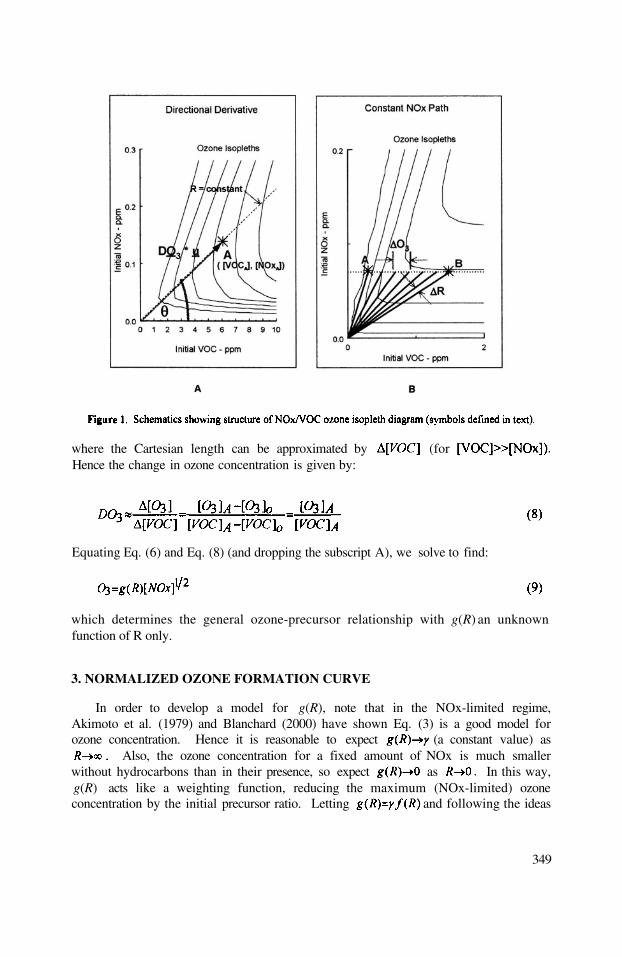
where the Cartesian length can be approximated by (forHence the change in ozone concentration is given by:
In order to develop a model for g(R), note that in the NOx-limited regime,Akimoto et al. (1979) and Blanchard (2000) have shown Eq. (3) is a good model forozone concentration. Hence it is reasonable to expect (a constant value) as
Also, the ozone concentration for a fixed amount of NOx is much smallerwithout hydrocarbons than in their presence, so expect as In this way,g(R) acts like a weighting function, reducing the maximum (NOx-limited) ozoneconcentration by the initial precursor ratio. Letting and following the ideas
349
Equating Eq. (6) and Eq. (8) (and dropping the subscript A), we solve to find:
3. NORMALIZED OZONE FORMATION CURVE
which determines the general ozone-precursor relationship with g(R) an unknownfunction of R only.
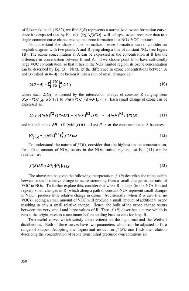
350
of Sakamaki et al. (1982), we find f (R) represents a normalized ozone formation curve,since it is expected that by Eq. (9), will collapse ozone-precursor data to asingle common curve characterizing the ozone formation of a NOx-VOC mixture.
To understand the shape of the normalized ozone formation curve, consider anisopleth diagram with two points A and B lying along a line of constant NOx (see Figure1B). The ozone concentration at A can be expressed as the concentration at B less thedifference in concentration between B and A. If we choose point B to have sufficientlylarge VOC concentration, so that it lies in the NOx limited region, its ozone concentrationcan be described by Eq. (3). Next, let the difference in ozone concentrations between Aand B (called ) be broken it into a sum of small changes i.e.:
where each is formed by the intersection of rays of constant R ranging fromto Each small change of ozone can be
expressed as:
and in the limit as (with as) the concentration at A becomes:
To understand the nature of f '(R), consider that the highest ozone concentration,for a fixed amount of NOx, occurs in the NOx-limited region, so Eq. (11) can berewritten as:
The above can be given the following interpretation: f ' (R) describes the relationshipbetween a small relative change in ozone stemming from a small change in the ratio ofVOC to NOx. To further explore this, consider that when R is large (in the NOx-limitedregion), small changes in R (which along a path of constant NOx represent small changesin VOC), produce little relative change in ozone. Additionally, when R is zero (i.e. noVOCs), adding a small amount of VOC will produce a small amount of additional ozoneresulting in only a small relative change. Hence, the bulk of the ozone change occursbetween the very small and large values of R. Thus, f ' (R) describes a curve which iszero at the origin, rises to a maximum before tending back to zero for large R.
Two useful curves which satisfy above criteria are the lognormal and the Weibulldistributions. Both of these curves have two parameters which can be adjusted to fit arange of shapes. Adopting the lognormal model for f ' (R), one finds the relationdescribing the concentration of ozone from initial precursor concentrations is:

For the Weibull, one obtains.
which is exactly the form suggested by Chang and Rudy (1993) (using the substitutionand developed through a semi-empirical analysis of smog chamber data.
Both curves have 2 unknown parameters which are dependent on the VOC mixture.
4. AGREEMENT WITH MODEL OUTPUT
An example of the Weibull and Lognormal models are shown in Figure 2 A. Modeloutput was obtained from an OZIPR simulation using the CAL mechanism with VOCspeciation given by Chang and Rudy (1990) and no dilution. The two parameters in eachmodel were determined by a non-linear optimisation. Figure 2B shows how thelognormal model characterises ozone formation. The solid lines represent isopleths fromthe OZIPR simulation, the dashed lines are isopleths based on Eq. (14). The correlationcoefficient between the two sets of isopleths is
5. HYDROCARBON REACTIVITIES
Another motivation for ozone-precursor research involves determining whichcompounds have a greater propensity for ozone formation. To measure the ozoneforming capability of VOCs, numerous reactivity scales have been developed (Carter,1994) and having an analytic model for ozone formation allows one to derive functionalforms for these scales.
5.1 Maximum Ozone Reactivity (MOR)
The MOR refers to the situation where initial concentrations produce themaximum ozone levels for an initial VOC mixture. The resulting ratiocorresponds to the ridgeline as defined by The lognormal modelgives the following expression for this ridgeline
351
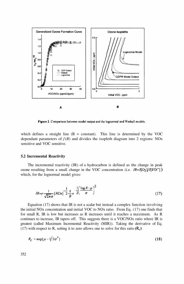
The incremental reactivity (IR) of a hydrocarbon is defined as the change in peakozone resulting from a small change in the VOC concentration (i.e.which, for the lognormal model gives:
Equation (17) shows that IR is not a scalar but instead a complex function involvingthe initial NOx concentration and initial VOC to NOx ratio. From Eq. (17) one finds thatfor small R, IR is low but increases as R increases until it reaches a maximum. As Rcontinues to increase, IR tapers off. This suggests there is a VOC/NOx ratio where IR isgreatest (called Maximum Incremental Reactivity (MIR)). Taking the derivative of Eq.(17) with respect to R, setting it to zero allows one to solve for this ratio
352
which defines a straight line (R = constant). This line is determined by the VOCdependant parameters of f (R) and divides the isopleth diagram into 2 regions: NOxsensitive and VOC sensitive.
5.2 Incremental Reactivity

The EBIR refers to the condition where the initial NOx concentrations are adjustedso that the change in ozone due to a small change in VOC equals the change in ozone to asmall change in NOx. Taking the derivative of Eq. (14) with respect to both NOx andVOC and equating the two gives the following expression:
Which again defines a straight line determined by the ratio and is uniquely determinedby the two parameters. A sketch of changing reactivities against changing NOxconcentrations was produced by Carter in his paper (1994) and is reproduced in Figure 3.A graph of the change in ozone with respect to VOC and generated using thelognormal model is shown in Figure 4. The three ratios (MOR, MIR, EBIR) are markedon the graph. The data are not plotted against the initial ratio of butagainst ‘scaled’ - defined as the ratio of initial to the amount of requiredto produce the maximum ozone concentration (for a fixed amount of VOC). Thesecurves clearly capture the ozone dependence sketched by Carter (1994) and have theadvantage of being generated by an objective, theoretically developed model.
353
This shows the critical ratio is dependent, again, on only the two parameters of f (R).Further analysis using the lognormal model, reveals that must always be less than(independent of VOC) consistent with modelling by Carter and Atkinson (1989).
5.3. Equal Benefit Incremental Reactivity (EBIR)
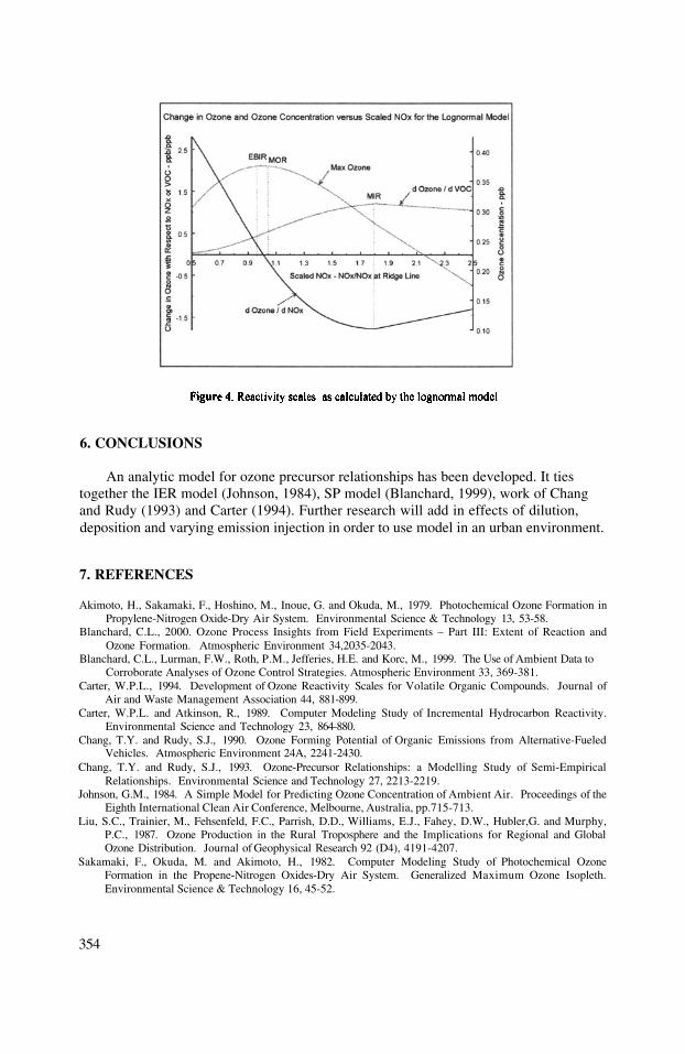
An analytic model for ozone precursor relationships has been developed. It tiestogether the IER model (Johnson, 1984), SP model (Blanchard, 1999), work of Changand Rudy (1993) and Carter (1994). Further research will add in effects of dilution,deposition and varying emission injection in order to use model in an urban environment.
Akimoto, H., Sakamaki, F., Hoshino, M., Inoue, G. and Okuda, M., 1979. Photochemical Ozone Formation inPropylene-Nitrogen Oxide-Dry Air System. Environmental Science & Technology 13, 53-58.
Blanchard, C.L., 2000. Ozone Process Insights from Field Experiments – Part III: Extent of Reaction andOzone Formation. Atmospheric Environment 34,2035-2043.
Blanchard, C.L., Lurman, F.W., Roth, P.M., Jefferies, H.E. and Korc, M., 1999. The Use of Ambient Data toCorroborate Analyses of Ozone Control Strategies. Atmospheric Environment 33, 369-381.
Carter, W.P.L., 1994. Development of Ozone Reactivity Scales for Volatile Organic Compounds. Journal ofAir and Waste Management Association 44, 881-899.
Carter, W.P.L. and Atkinson, R., 1989. Computer Modeling Study of Incremental Hydrocarbon Reactivity.Environmental Science and Technology 23, 864-880.
Chang, T.Y. and Rudy, S.J., 1990. Ozone Forming Potential of Organic Emissions from Alternative-FueledVehicles. Atmospheric Environment 24A, 2241-2430.
Chang, T.Y. and Rudy, S.J., 1993. Ozone-Precursor Relationships: a Modelling Study of Semi-EmpiricalRelationships. Environmental Science and Technology 27, 2213-2219.
Johnson, G.M., 1984. A Simple Model for Predicting Ozone Concentration of Ambient Air. Proceedings of theEighth International Clean Air Conference, Melbourne, Australia, pp.715-713.
Liu, S.C., Trainier, M., Fehsenfeld, F.C., Parrish, D.D., Williams, E.J., Fahey, D.W., Hubler,G. and Murphy,P.C., 1987. Ozone Production in the Rural Troposphere and the Implications for Regional and GlobalOzone Distribution. Journal of Geophysical Research 92 (D4), 4191-4207.
Sakamaki, F., Okuda, M. and Akimoto, H., 1982. Computer Modeling Study of Photochemical OzoneFormation in the Propene-Nitrogen Oxides-Dry Air System. Generalized Maximum Ozone Isopleth.Environmental Science & Technology 16, 45-52.
354
6. CONCLUSIONS
7. REFERENCES

How do you derive the isopleths used in your simplified model ?
Isopleths are developed from plotting the ozone-precursorrelationship. The unknown parameters in the model are found fromregression to the model output. This then allows the ozone-precursorrelationship to be fully defined and isopleths created.
355
A. HANSEN
DISCUSSION
B. AINSLIE

This page intentionally left blank

ON THE RELATIONSHIP BETWEEN THELAGRANGIAN AND EULERIAN TIME SCALE: APRELIMINARY EVALUATION WITH LES DATA
U. Rizza1, D. Anfossi2, C.Mangia1, G. A.Degrazia3
1.INTRODUCTION
In the Planetary Boundary Layer (PBL), Eulerian (i.e, fixed point) wind measurementis the only type of measurement which is generally feasible on a routinely way. However,when studying the atmospheric diffusion, interest focuses on the variation of velocity withtime which would be observed following the air motion (Lagrangian description). Thusthe basic problem of relating Eulerian and Lagrangian statistics (autocorrelationfunctions, structure functions, spectra and, in particular, time scales arises. Despiteof substantial experimental and theoretical efforts (see, for instance: Gifford, 1955; Hayand Pasquill, 1959; Wandel and Kofoed, 1962; Corrsin, 1963; Saffman, 1963; Smith,1967; Angell et1 al., 1971; Hanna, 1981; Li and Meroney, 1985; Squires and Eaton, 1991;Wang et al., 1995; Querzoli, 1996; Koeltzsch, 1999; Phillips, 2000), a complete
theoretical derivation of the ratio in the PBL is not yet available. At present,
most workers use the relationship
1Consiglio Nazionale delle Ricerche, Istituto ISIATA, Lecce, Italy, Consiglio
Nazionale delle Ricerche, Istituto di Cosmogeofisica, Turin, Italy, UniversidadeFederal de Santa Maria, Departamento de Física, Santa Maria, RS, Brazil
Air Pollution Modeling and Its Application XV, Edited byBorrego and Schayes, Kluwer Academic/Plenum Publishers, New York, 2002 357
2
3
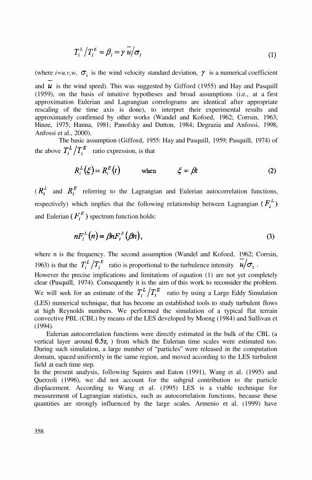
(where i=u,v,w, is the wind velocity standard deviation, is a numerical coefficient
and is the wind speed). This was suggested by Gifford (1955) and Hay and Pasquill(1959), on the basis of intuitive hypotheses and broad assumptions (i.e., at a firstapproximation Eulerian and Lagrangian correlograms are identical after appropriaterescaling of the time axis is done), to interpret their experimental results andapproximately confirmed by other works (Wandel and Kofoed, 1962; Corrsin, 1963;Hinze, 1975; Hanna, 1981; Panofsky and Dutton, 1984; Degrazia and Anfossi, 1998,Anfossi et al., 2000).
The basic assumption (Gifford, 1955: Hay and Pasquill, 1959; Pasquill, 1974) of
the above ratio expression, is that
358
( and referring to the Lagrangian and Eulerian autocorrelation functions,
respectively) which implies that the following relationship between Lagrangian
and Eulerian spectrum function holds:
where n is the frequency. The second assumption (Wandel and Kofoed, 1962; Corrsin,
1963) is that the ratio is proportional to the turbulence intensity
However the precise implications and limitations of equation (1) are not yet completelyclear (Pasquill, 1974). Consequently it is the aim of this work to reconsider the problem.
We will seek for an estimate of the ratio by using a Large Eddy Simulation
(LES) numerical technique, that has become an established tools to study turbulent flowsat high Reynolds numbers. We performed the simulation of a typical flat terrainconvective PBL (CBL) by means of the LES developed by Moeng (1984) and Sullivan et(1994).
Eulerian autocorrelation functions were directly estimated in the bulk of the CBL (avertical layer around ) from which the Eulerian time scales were estimated too.During such simulation, a large number of “particles” were released in the computationdomain, spaced uniformly in the same region, and moved according to the LES turbulentfield at each time step.In the present analysis, following Squires and Eaton (1991), Wang et al. (1995) andQuerzoli (1996), we did not account for the subgrid contribution to the particledisplacement. According to Wang et al. (1995) LES is a viable technique formeasurement of Lagrangian statistics, such as autocorrelation functions, because thesequantities are strongly influenced by the large scales. Armenio et al. (1999) have

discussed the effects of the subgrid velocity fluctuations on particle motion finding that itcan generally be disregarded. Nieuwstadt and Meeder (1997) included in their LES thesubgrid contribution to the Lagrangian particle motion. This aspect will be closelyconsidered in the future development of the present analysis. From the ensemble ofcomputed trajectories the Lagrangian autocorrelation function and time scale werederived. In the present paper the first results of this work are presented.
2. AN OVERVIEW OF SIMULATION PERFORMED
The LES model used in the present study was developed by C.H. Moeng at NCARand described in detail by Moeng (1984) and Sullivan et al (1994). The numerical schemeis pseudo-spectral in the horizontal, and second-order centered finite difference in thevertical direction. The grid resolution is in a (10x10x2) km domain. With suchresolution the sub-grid eddies are of such small size that they receive their own energyfrom the energy cascade, thus being less sensitive to flow geometry. The eddy viscositymodel is the new formulation proposed by Sullivan et al (1994). This in particular allowsbetter matching with surface layer similarity theory as showed by the authors.Turbulent regimes are generated by varying geostrophic wind and surface vertical heatflux. Moeng and Sullivan (1994) made a sensitivity analysis over such forcing parametersgenerating different turbulent regimes. We utilized data from their named experiment B toinitialize our simulation. The initial and calculated CBL parameters are depicted in thefollowing Table 1.:
Where is the initial inversion height, are the components of geostrophic
wind, is the surface temperature flux, the friction velocity and finally
is the large-eddy turnover time. Our simulation lasted around 15 turnover time to reach anearly statistically stationary CBL. In such turbulent field the particles will be injectedfrom uniformly distributed grid points in the mid-CBL.
359
2.1 Les Model
2.2 Eulerian statistics
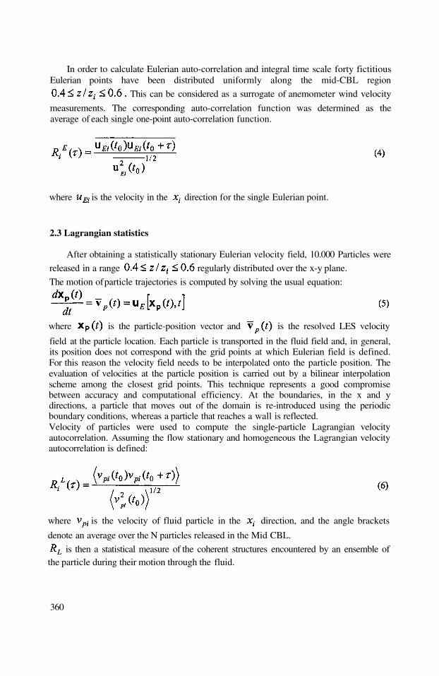
In order to calculate Eulerian auto-correlation and integral time scale forty fictitiousEulerian points have been distributed uniformly along the mid-CBL region
This can be considered as a surrogate of anemometer wind velocity
measurements. The corresponding auto-correlation function was determined as theaverage of each single one-point auto-correlation function.
where is the velocity in the direction for the single Eulerian point.
where is the velocity of fluid particle in the direction, and the angle brackets
denote an average over the N particles released in the Mid CBL.
is then a statistical measure of the coherent structures encountered by an ensemble ofthe particle during their motion through the fluid.
360
After obtaining a statistically stationary Eulerian velocity field, 10.000 Particles were
released in a range regularly distributed over the x-y plane.
The motion of particle trajectories is computed by solving the usual equation:
where is the particle-position vector and is the resolved LES velocity
field at the particle location. Each particle is transported in the fluid field and, in general,its position does not correspond with the grid points at which Eulerian field is defined.For this reason the velocity field needs to be interpolated onto the particle position. Theevaluation of velocities at the particle position is carried out by a bilinear interpolationscheme among the closest grid points. This technique represents a good compromisebetween accuracy and computational efficiency. At the boundaries, in the x and ydirections, a particle that moves out of the domain is re-introduced using the periodicboundary conditions, whereas a particle that reaches a wall is reflected.Velocity of particles were used to compute the single-particle Lagrangian velocityautocorrelation. Assuming the flow stationary and homogeneous the Lagrangian velocityautocorrelation is defined:
2.3 Lagrangian statistics

3. PRELIMINARY RESULTS
Figura 1 shows the Eulerian and Lagrangian autocorrelation functions for eachcomponent. It is evident that Eulerian velocity correlations are always smaller than theLagrangian ones for small time separations. Concerning the estimation of time scales,both Eulerian and Lagrangian, three methods are generally used in the literature: best fitof autocorrelogram, integration of autocorrelogram and determination of the time atwhich the autocorrelogram decreases to 1/e. In the first and third method, an exponentialdecay for is assumed. Hanna (1981) discussed the second and third method only.
Since the second method was found to be less reliable, because the observedautocorrelogram does not generally approach zero at the largest time lags, Hanna chosethe 1/e method. Moore et al. (1985) tested all the three methods and found that the firstone (best fit) was the more accurate. Anfossi et al. (2000) choose the first one. Therefore,
in the present analysis we evaluated and from the best fit of autocorrelation
functions, assumed exponential (Figure 2).
In Table 2 there are summarised the numerical values of Lagrangian/Eulerian time scaleand the value of the ratio TL/TE. Results obtained are in the range of values found inliterature. However they have to be considered preliminary. Further investigations andsimulations have been planed in order to analyse the dependence on stability for the threecomponents and the subgrid contributions.
361
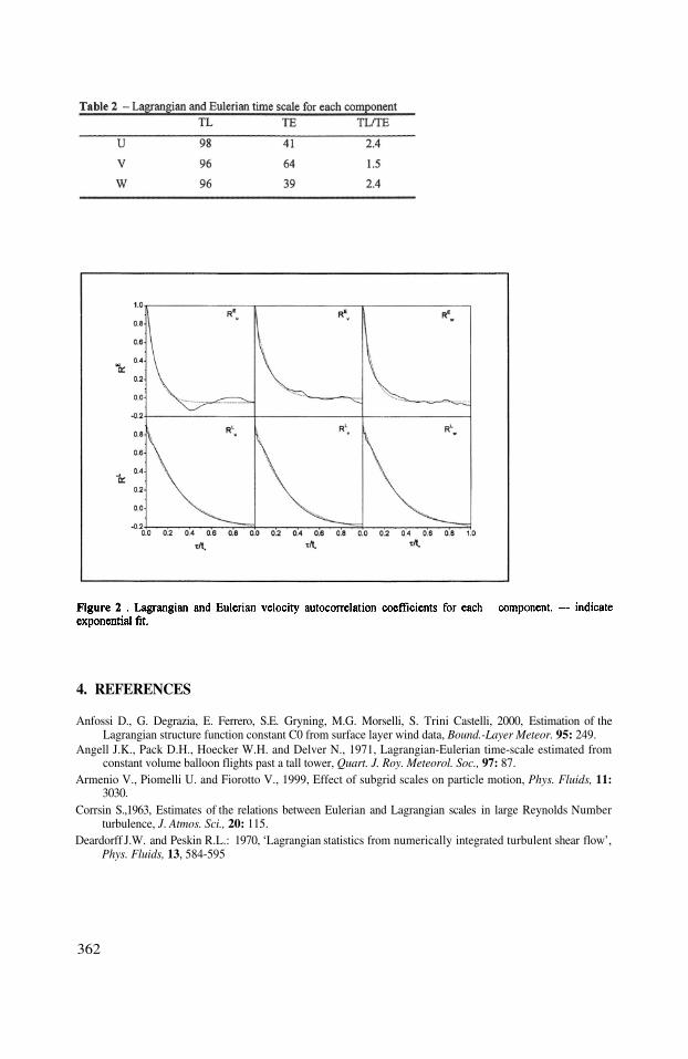
Anfossi D., G. Degrazia, E. Ferrero, S.E. Gryning, M.G. Morselli, S. Trini Castelli, 2000, Estimation of theLagrangian structure function constant C0 from surface layer wind data, Bound.-Layer Meteor. 95: 249.
Angell J.K., Pack D.H., Hoecker W.H. and Delver N., 1971, Lagrangian-Eulerian time-scale estimated fromconstant volume balloon flights past a tall tower, Quart. J. Roy. Meteorol. Soc., 97: 87.
Armenio V., Piomelli U. and Fiorotto V., 1999, Effect of subgrid scales on particle motion, Phys. Fluids, 11:3030.
Corrsin S.,1963, Estimates of the relations between Eulerian and Lagrangian scales in large Reynolds Numberturbulence, J. Atmos. Sci., 20: 115.
Deardorff J.W. and Peskin R.L.: 1970, ‘Lagrangian statistics from numerically integrated turbulent shear flow’,Phys. Fluids, 13, 584-595
362
4. REFERENCES

Degrazia G.A. and Anfossi D., 1998, Estimation of the Kolmogorov constant from classical statistical
diffusion theory, Atmos. Environ., 32: 3611.Gifford F.A., 1955, A simultaneous Lagrangian-Eulerian turbulence experiment, Monthly Weather Rev., 83:
293.Hanna S.R.: 1981, Lagrangian and Eulerian time-scale in the daytime boundary layer. J. Appl. Meteorol.,
20:242.Hay J.S. and Pasquill F.:1959, ‘Diffusion from a continuous source in relation to the spectrum and scale of
turbulence’. Atmospheric Diffusion and Air Pollution, F.N. Frenkiel and P.A. Sheppard eds., Advances inGeophysics, 6, 345, Academic Press
Hinze J.O., 1975, Turbulence, Mc Graw Hill, 790 ppKoeltzsch K, 1999, On the relationship between the Lagrangian and Eulerian time scale, Atmos. Environ. 33:
117.Li W.W. and Meroney R.N., 1985, Re-examination of Eulerian-Lagrangian turbulence relationships, Atmos.
Environ., 19: 853.Moeng C.H., 1984, A Large Eddy Simulation Model for the Study of Planetary Boundary Layer Turbulence, J.
of Atmos. Sci., 41, 13: 2052.Moeng C.H. and Sullivan, P.P, 1994, A comparison of shear and buoyancy driven Planetary Boundary Layer
flows, J. of Atmos. Sci. 51, 7: 999.Nieuwstadt F.T.M. and Meeder J.P., 1997, Large-Eddy simulation of air pollution dispersion: a review, in New
tools in turbulence modelling, O. Metais and J. Ferziger editors, Lecture 13, 265-280Panofsky H.A. and Dutton J.A., 1984, Atmospheric Turbulence - Model and methods for Engineering
applications, John Wiley and Sons, New York, 397 ppPasquill F., 1974: ‘Atmospheric diffusion’, Wiley & Sons, 429 ppPhillips W.R.C., 2000, Eulerian space-time correlations in turbulent shear flows, Phys. Fluids, 12: 205.Querzoli G.: 1996, ‘A Lagrangian study of particle dispersion in the unstable boundary layer’, Atmos. Environ.
30: 2821.Saffman P.O.,: 1963, An approximate calculation of the Lagrangian autocorrelationcoefficient for stationary
homogeneous turbulence, Applied Science Res., 11, 245Smith F.B., 1967, Eulerian and Lagrangian time-scale relationship in one-dimensional turbulence, USAEC
Meteorological Information Meeting, Chalk River, Canada (AECL-2787), 476-483Squires K.D. and Eaton J.K., 1991, Lagrangian and Eulerian statitistics obtained from direct numerical
simulations of homogeneous turbulence, Phys. Fluids, A3: 130.Sullivan, P.P., Mc Williams, J.C., Moeng , C.H. 1994, A subgrid-scale model for large-eddy simulation of
planetary boundary layer flows’, Bound.- Layer Meteor., 71, 247.Wandel C.F. and Kofoed-Hansen O.,1962, On the Eulerian-Lagrangian transform in the statistical theory of
turbulence, J. Geophys. Res., 76: 3089.Wang Q., Squires K.D. and Wu X., 1995, Lagrangian statistics in turbulent channel flow, Atmos. Environ. 29:
2417.
363

DISCUSSION
As in the case of the autocorrelation length sales these should be astrong height dependency of the Eulerian time scale. Which resultshereon you have found ? To which height your presented findingsare related to ?
As I mentioned in my presentation, Eulerian measurements werecarried out in the layer and the Lagrangian trajectoriesstarted in the same layer.
A. BAKLANOV Why did you study the CBL cases only ? I think, the SBL case ismore interesting and important) for the relationship study (as 1remember, the LES datasets of Mocny and Sullivan include someSBL cases as well). The most interesting case would be the SBLcapped by free-flow stability with possible penetration of the internalgravity waves in the SBL.
We considered CBL cases only till now but we will consider stablecases also in the near future. We agree that stable cases are importantfor the reasons you mention.
364
O. HELLMUTH
D. ANFOSSI
D. ANFOSSI

CALMET (Scire et al., 1999) is a diagnostic meteorological model that parametrisesslope flows, kinematic terrain effects, terrain blocking effects, and includes a divergenceminimisation procedure. CALMET contains also a micrometeorological model for thecalculation of the planetary boundary layer parameters both overland and overwater.Since 1999 CALMET is the diagnostic meteorological model suggested by the US-EPA.
This work presents new algorithms thought to overcome some limitations currentlypresent into the model. The modifications concern the energy balance equation, thetemperature interpolation and the PBL height calculation. The original version ofCALMET considers only the direct radiation impinging over the ground and does notinclude shadowing effects. New routines were added in order to take into accounttopography induced shadows and to calculate direct, diffuse and reflected radiation.Moreover CALMET determines ground temperature at grid points doing a pure spatialinterpolation of measurements that does not consider the different heights above the sealevel of the points themselves. New routines were added to take into account the verticaltemperature gradient, topography properties such as slope and aspect and the vegetationcover. Finally the algorithm originally present in CALMET to calculate the planetaryboundary layer height were substituted with those described by Batcharova and Gryning(1991) for daytime conditions and by Zilitinkevich (1989) for nighttime conditions. Thealgorithms for the calculation of the PBL parameters will be not described in thefollowing of this paper. A comprehensive description of these algorithms can be foundfor example in Seibert et al. (2000).
* Maffeis G., TerrAria srl - via Zarotto 6 - 20124 Milano – Italy. Bellasio R. Enviroware srl - CentroDirezionale Colleoni, Andromeda 1 - 20041 Agrate Brianza (MI) – Italy. Scire J.S. Earth Tech, Inc. - 196Baker Avenue – Concord, MA 01742 – USA. Longoni M.G. TerrAria srl - via Zarotto 6 - 20124 Milano –Italy. Bianconi R. Enviroware srl - Centro Direzionale Colleoni, Andromeda 1 - 20041 Agrate Brianza (MI)– Italy. Quaranta N. Office for Risk Prevention, Civil Protection, Lombardy Region - Via Fara, 26 - 20124Milano – Italy.
Air Pollution Modeling and Its Application XV, Edited byBorrego and Schayes, Kluwer Academic/Plenum Publishers, New York, 2002
NEW ALGORITHMS FOR THE DETERMINATION OFSOLAR RADIATION, SURFACE TEMPERATURE AND
PBL HEIGHT IN CALMET
Maffeis G., Bellasio R., Scire J.S., Longoni M.G., Bianconi R., Quaranta N.*
1. INTRODUCTION
365

The effect of the new algorithms introduced in CALMET is particularly significantfor model applications over complex topography. The results of a simulation in thenorthern part of Italy, where the presence of the Alpes draws a very complex terrain, arepresented.
A schematic representation of the modifications introduced in CALMET is presentedin Figure 1.
During the setup process some properties of the topography, such as slope (S), aspect(A), horizon angle and view factor are calculated as explained for example in Dozier etal. (1981), Dozier and Frew (1990) and Gallant and Wilson (1996). For each hour ofsimulation and for each grid cell, the position of the sun is calculated. In order todetermine if a given grid cell is shadowed by other topography, the horizon angle alongthe direction of the solar azimut is compared with the solar zenith. If the horizon angleexceeds the solar zenith, the cell is shadowed by the surrounding topography. In that casethe direct component of the short wave radiation is null. The radiation balance is obtainedconsidering both short wave and long wave ratiation. The latter is obtained using theatmospheric temperature calculated with the new interpolation algorithms that consideralso terrain elevation and topography properties. Finally, solving the energy balanceequation it is possible to obtain the scale parameters of the planetary boundary layer.
366
2. BRIEF DESCRIPTION OF THE MODIFICATIONS

367
3. RADIATION BALANCE
The radiation balance over any surface, with arbitrary orientation in the space, can bewritten as (Moore et al., 1993):
Where is the net radiation is the albedo, is the direct short waveradiation is the diffuse short wave radiation is the reflectedshort wave radiation is the emissivity of the ground, is the long waveincoming radiation and is the long wave outcoming radiation
The outcoming long wave radiation is given by the well known Stefan Boltzmannrelation:
where is the stefan Boltzman constant and is the groundtemperature (K). The incoming long wave radiation is given by:
where is the atmospheric emissivity, is the atmospheric temperature and is theview factor. The atmospheric emissivity is a function of atmospheric temperature, vapourpressure of atmospheric water and cloud cover. The view factor indicates the fraction ofsky visible from a specific point; it depends from surface slope, and topography aroundthe point. A fast algorithm for the calculation of the view factor was presented by Dozierand Frew (1990).
Since ground temperature is not always available, and since it is not available inCALMET, the fourth power of that variable can be substituted by the fourth power of theatmospheric temperature plus the correction term as done in Holtslag and vanUlden (1983). With this assumption the net radiation over a surface is written as:
In order to evaluate the net radiation, expressions for the short wave radiationcomponents are needed. These expressions require the knowledge of properties of theactual topography such as slope and aspect that can be calculated as illustrated by Gallantand Wilson (1996).
Entering into the atmosphere the short wave radiation is attenuated along its opticalpath. An equation for the attenuation factor is (Thornton and Running, 1998):
368
where is the attenuation factor at nadir (typically 0.6), is the solar zenith, isthe non dimensional optical path and p and are the atmospheric pressures at currentheight and at sea level respectively. More complete formulation should consider alsosome pollutants (e.g. particulate matter) and water vapour.
The direct short wave radiation impinging on a sloping surface is written as:
where is the atmospheric transmission coefficient for the diffuse radiation (Liu andJordan, 1960), is the circumsolar coefficient (typically 0.25), Z is the local zenith withrespect to the sloping surface (Gallant and Wilson, 1996), is the solar constantcorrected by the orbital vector (i.e. the ratio between the actual sun-earth distance andtheir average distance) and is an attenuation factor due to cloud cover. This equation isvalid if current topography is not shadowed by the surrounding topography, otherwise
Finally the diffuse and reflected components of the short wave radiationare respectively given by
4. TEMPERATURE INTERPOLATION
Present version of CALMET mainly calculates surface temperature field with aspatially weighted average of surface station temperature observations, where thedimensionless weighting factors are based on the distance r from the (i,j)th grid cell to thevarious surface meteorological stations (1/r or function could be used). Thisprocedure is correct on an almost homogenous terrain, but begins to fail, for istance, in acomplex terrain (close grid points along the horizontal direction could have differenttemperature if they have different altitudes).
The newly developed algorithms try to overcome these limitations taking intoaccount the following parameters:
different altitude respect to reference monitoring station;temperature vertical gradient;geometric characteristics (slope, aspect ..) of each grid cell;vegetation coverage.
Moore et al. (1993) present a specific algorithm to calculate temperature at adifferent altitude within a valley, where only one measure point is present. The followingsimple equation is proposed:

369
where is the unknown atmospheric temperature (K) at a altitude (m), is themeasured atmospheric temperature (K) at a altitude (m), is the verticaltemperature gradient (K/km), C is a constant usually equal to one, and are,respectively, maximum Leaf Area Index and its value at is the ratio between netshort radiation on the real surface (with its slope and aspect) and on an horizontal freesurface. Temperature, following these two equations, increases for South orientedsurfaces greater than one). Moreover the correction is a function of the leaf coverage(Running et al., 1987): surfaces poor of vegetation respect to used, equalto 10) obtain the maximum temperature increase or decrease. Net short radiation takesinto account the surface albedo, the reflected and diffuse radiation term. The difference inaltitude is transformed in difference in temperature through the vertical temperaturegradient.
To eliminate the discontinuity between the two previous equations when anew formulation has been introduced:
It should be noted that all these formulations do not apply to night-time conditions,when equal zero. During night a simplified formulation derived from the previous oneis used: the second term of the sum is set equal to zero.
New CALMET temperature computation methodology includes the following steps:all temperature measurements are carried back to a reference altitude (zero meters)and to a reference vegetation coverage equal to zero), through the last equationwhere the vertical temperature gradient used in the equation is calculated byCALMET for each hour from the measured vertical profiles;the original CALMET interpolation scheme is now used for the “referenced”temperature (a virtual homogeneous terrain has been built);at the end of the interpolation, temperatures are recomputed correcting for actualcondition of altidude, slope, aspect and vegetation of the specific grid cell (inversetransformation of step 1).
5. FIRST APPLICATION TO A COMPLEX TERRAIN DOMAIN
Figure 2 represents topography of the domain used for the test of the new CALMETparametrization. The domain is positioned in the Northern part of Italy, centered onLombardy Region. The 46x41 cells of range from zero to more than 3000 metersof altitudes, passing through a plain rural landuse in the South -Pianura Padana, a verydense metropolitan area in the middle -Milan, ending with mountain and valleys in the
1
2
3

North -the Alps. Simulation day is the of July 1994 during a photochemical smogepisode studied by De Martini et al. (1998).
Figure 3 and Figure 4 show direct and diffuse radiation computed with the newalgorithms during the of July. Some interesting phenomena should be remarked:
during the first hours of the day (6 a.m.) the diffuse radiation is an important partof the total short radiation (diffuse contribution is almost equal to direct onewhere the land is flat); the situation is very different in the afternoon (2 p.m.)when direct radiation prevails;diffuse radiation has a very different spatial pattern respect to the direct one: thefirst is almost spatially homogeneous with a longitudinal effect due to sunaltitude; the second gives prominence to surfaces with favourable slope andaspect respect to the sun angle.
370

Figure 5 shows the surface temperature computed by CALMET. The orographiceffect is evident since mountains are the coldest part of the domain. A smoothing effect,respect to stations influence, is another point in favour of this new interpolation scheme.
371
6. ACKNOWLEDGMENTS
The authors wish to thank Dr. S. W. Running and Dr. J. Dozier for the useful materialreceived.
5. REFERENCES
Batcharova E. and Gryning S.-E. (1991) Applied model for the growth of the daytime mixed layer. BoundaryLayer Meteorology, 56, 261-274.
De Martini A., Pasi F., Maffeis G., Longoni M.G., Tamponi M., Graziani G., Lanzani G. (1998) Modellingphotochemical smog episodes in Lombardy Region. 23rd NATO/CCMS International Technical Meetingon Air Pollution Modeling and Its Application Varna – Bulgaria.
Dozier J., Bruno J. and Downey P. (1981) A faster solution of the horizon problem. Comput. Geosci., 7, 145-151
Dozier J. and Frew J. (1990) Rapid calculation of terrain parameters for radiation modeling from digitalelevation model data. IEEE Transactions on Geoscience and Remote Sensing, 28, 963-969.
Gallant, J.C. and Wilson, J.P. (1996) TAPES-G: A grid-based terrain analysis program for the environmentalsciences. Computers and Geosciences vol. 22 no. 7 pp 713-722
Holtslag A.A.M. and van Ulden A.P. (1983) A simple scheme for daytime estimates of the surface fluxes fromroutine weather data. J. Of Climate and Applied Meteorology, Vol. 22, N. 4, 517-529.
Liu, B. Y. H. and Jordan, R. C. (1960) The interrelationship and characteristic distribution of direct, diffuse, andtotal solar radiation. Solar Energy 4:1-19.
Moore I.D., Norton T.W. and Williams J.E. (1993) Modeling environmental heterogeneity in forestedlandscapes. Journal of Hydrology, 150, 717-747
Running S.W., Nemani R.R. and Hungerford R.D. (1987) Extrapolation of synoptic meteorological data inmountainous terrain and its use for simulating forest evapotranspiration and photosynthesis. Can. J. For.Res., 17, 472-483.
Scire J.S., Robe F.R., Fernau M.E. and Yamartino R.J. (1999) A user’s guide for the CALMET meteorologicalmodel (Version 5.0). Earth Tech Inc., September 1999.
Seibert P., Beyrich F., Gryning S.-E. Joffre S., Rasmussen A. and Tercier P. (2000) Review andintercomparison of operational methods for the determination of the mixing height. AtmosphericEnvironment, 34, 7, 1001-1027.
Zilitinkevich S.S. (1989) Velocity profile, the resistance law and the dissipation rate of mean flow kineticenergy in a neutrally and stably stratified planetary boundary layer. Boundary Layer Meteorology, 46,367-387.
372

DISCUSSION
O. HELLMUTH
J.S. SCIRE
To my understanding your refined radiation approach has beenapplied to the grid-resolved part of the model topography (azimuth,inclination, slope of terrain). What do you think about theimportance to apply your approach also to the subgrid-scaletopography in a sense comparable to the blending height concept for“flux averaging” ? (averaging of subgridscale, terrain corrected netradiation values in very complex regions ?)
The approach in CALMET is applied to the grid resolvedtopography. However, with a diagnostic model it is possible toincrease the grid resolution down to 50-100 m cells in order toexplicitly evaluate small scale effects. This is usually not a practicalway for prognostic models.We apply a simple approach to determine mixing heights, whichrespond to the heat flux across many grid cells, if the grid spacing issmall. The mixing heights is first computed at each grid cell usingthe local heat flux. An upwind-looking, spatially averaged mixingheight is then computed to “blend” the effects of upwind grid cellswith different heat flux characteristics.
373

This page intentionally left blank
USE OF NEURAL NETWORKS IN THE FIELD OF AIRPOLLUTION MODELLING
Marija Zlata Boznar and Primoz Mlakar*
1. ABSTRACT
Different possibilities of using artificial neural networks are described. There are twodifferent types of neural networks that are suitable for the use in the field of air pollutionmodelling. The first is the multi-layer Perceptron neural network and similar structures.The second is the Kohonen neural network. Both structures are briefly described. Severalexamples using both tools are demonstrated.
In the case of prediction of sulphur dioxide concentrations over complex terrain wedeveloped a complete method of using a multi-layer Perceptron neural network includingfeature determination and pattern selection techniques that enhance the method’sefficiency. In past years other research groups obtained good results in similarapplications. Most of them dealt with ozone pollution over urban areas.
Multi-layer Perceptron neural networks can also be used in other applications. Twoapplications are explained: as a wind speed and direction forecasting tool in local scaleapplications over complex terrain, and as a SODAR measurements reconstruction tool.SODAR measurements on different layers above a basin were reconstructed from groundlevel wind measurements in the basin and on the hills.
The second tool described in this paper is the Kohonen neural network. This neuralnetwork is a self-organising classificator especially useful for cluster analysis.
Firstly it is explained how the Kohonen neural network was used to find significantwind fields over complex terrain on a small scale area. The wind field over the basin wasrepresented by six ground level wind measurements on the plain of the basin and on thehills. A very large set of measurements was examined in the study. The Kohonen neuralnetwork classified the data set into around thirty groups. To judge the quality of theclassification, wind roses were plotted for each measuring point using patterns from eachgroup. The graphical representation of selected groups proved the extreme efficiency ofthe classification.
The second efficient use of the Kohonen neural network was in the preparation phaseof multi-layer Perceptron neural network air pollution forecasting model construction.We developed a pattern selection technique based on the Kohonen neural network. In thepaper main guidelines for its use are given.
* Jozef Stefan Institute, Jamova 39, SI-1000 Ljubljana, Slovenia
Air Pollution Modeling and Its Application XV, Edited byBorrego and Schayes, Kluwer Academic/Plenum Publishers, New York, 2002 375
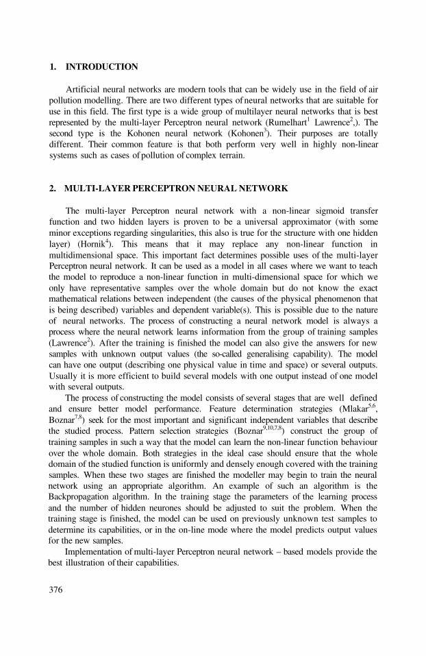
1. INTRODUCTION
Artificial neural networks are modern tools that can be widely use in the field of airpollution modelling. There are two different types of neural networks that are suitable foruse in this field. The first type is a wide group of multilayer neural networks that is bestrepresented by the multi-layer Perceptron neural network (Rumelhart1 Lawrence2,). Thesecond type is the Kohonen neural network (Kohonen3). Their purposes are totallydifferent. Their common feature is that both perform very well in highly non-linearsystems such as cases of pollution of complex terrain.
2. MULTI-LAYER PERCEPTRON NEURAL NETWORK
The multi-layer Perceptron neural network with a non-linear sigmoid transferfunction and two hidden layers is proven to be a universal approximator (with someminor exceptions regarding singularities, this also is true for the structure with one hiddenlayer) (Hornik4). This means that it may replace any non-linear function inmultidimensional space. This important fact determines possible uses of the multi-layerPerceptron neural network. It can be used as a model in all cases where we want to teachthe model to reproduce a non-linear function in multi-dimensional space for which weonly have representative samples over the whole domain but do not know the exactmathematical relations between independent (the causes of the physical phenomenon thatis being described) variables and dependent variable(s). This is possible due to the natureof neural networks. The process of constructing a neural network model is always aprocess where the neural network learns information from the group of training samples(Lawrence2). After the training is finished the model can also give the answers for newsamples with unknown output values (the so-called generalising capability). The modelcan have one output (describing one physical value in time and space) or several outputs.Usually it is more efficient to build several models with one output instead of one modelwith several outputs.
The process of constructing the model consists of several stages that are well definedand ensure better model performance. Feature determination strategies (Mlakar5,6,Boznar7,8) seek for the most important and significant independent variables that describethe studied process. Pattern selection strategies (Boznar9,10,7,8) construct the group oftraining samples in such a way that the model can learn the non-linear function behaviourover the whole domain. Both strategies in the ideal case should ensure that the wholedomain of the studied function is uniformly and densely enough covered with the trainingsamples. When these two stages are finished the modeller may begin to train the neuralnetwork using an appropriate algorithm. An example of such an algorithm is theBackpropagation algorithm. In the training stage the parameters of the learning processand the number of hidden neurones should be adjusted to suit the problem. When thetraining stage is finished, the model can be used on previously unknown test samples todetermine its capabilities, or in the on-line mode where the model predicts output valuesfor the new samples.
Implementation of multi-layer Perceptron neural network – based models provide thebest illustration of their capabilities.
376

2.1. Forecasting Air Pollutant Concentrations
The first detailed development of methodology was done for prediction of sulphurdioxide concentrations using multi-layer Perceptron neural networks (Boznar12). It wasapplied on air pollution measuring sites around a thermal power plant in very complexterrain. In this application, which was studied further in detail, measurements ofmeteorological parameters and pollutant concentrations at several automatic stations wereused to predict the pollutant concentration for one measuring interval in advance at onestation. For different stations different models were built (Boznar7,8 Mlakar12-14).
Similar applications are ones for prediction of ozone concentrations over urban areas(Yi15). Ozone seems to be a very good example, because its relations with other pollutantsand with meteorological parameters are highly non-linear and not all the coefficients arewell determined. A neural network-based model can overcome this problem by learningthe necessary information directly from the training samples.
Multi-layer Perceptron neural network-based models can also be applied to test caseslike Kincaid and others that are used for model verification. In such applications themodel should be constructed to reproduce the concentration at one or several samplingpoints (always one output per one sampling point). The inputs may be any of theavailable meteorological measurements and emission rates. The available data set shouldbe strictly divided into a training set (which also includes the optimising set) and a testingset. The results on the testing set given by the neural network-based model can becompared with the results of other models on the same data set. The problem is thatneural network-based model constructed in this way is only useful for the particularapplication and “palette” of meteorological situations that it has been trained with. It
377
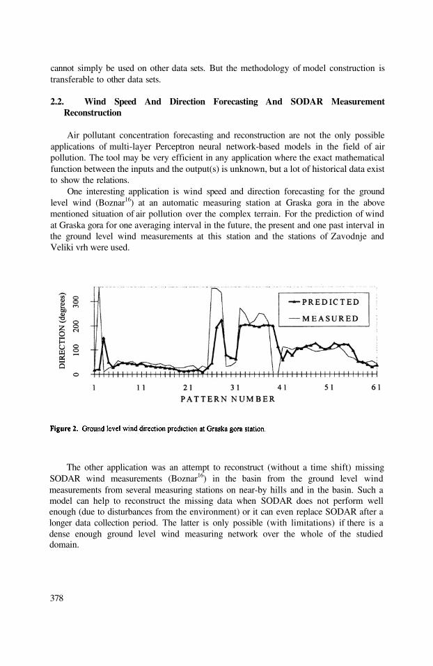
cannot simply be used on other data sets. But the methodology of model construction istransferable to other data sets.
2.2. Wind Speed And Direction Forecasting And SODAR MeasurementReconstruction
Air pollutant concentration forecasting and reconstruction are not the only possibleapplications of multi-layer Perceptron neural network-based models in the field of airpollution. The tool may be very efficient in any application where the exact mathematicalfunction between the inputs and the output(s) is unknown, but a lot of historical data existto show the relations.
One interesting application is wind speed and direction forecasting for the groundlevel wind (Boznar16) at an automatic measuring station at Graska gora in the abovementioned situation of air pollution over the complex terrain. For the prediction of windat Graska gora for one averaging interval in the future, the present and one past interval inthe ground level wind measurements at this station and the stations of Zavodnje andVeliki vrh were used.
The other application was an attempt to reconstruct (without a time shift) missingSODAR wind measurements (Boznar16) in the basin from the ground level windmeasurements from several measuring stations on near-by hills and in the basin. Such amodel can help to reconstruct the missing data when SODAR does not perform wellenough (due to disturbances from the environment) or it can even replace SODAR after alonger data collection period. The latter is only possible (with limitations) if there is adense enough ground level wind measuring network over the whole of the studieddomain.
378

3. KOHONEN NEURAL NETWORK
The second widely used tool, but one totally different from the multi-layerPerceptron neural network, is the Kohonen neural network (Kohonen3). This is a self –organising classificator. It is capable of finding groups of similar patterns (represented asmulti-dimensional vectors) in huge data sets. It is very important that the most suitablenumber of groups need not be known in advance. Therefore the tool can also be used inthe cases without a priori knowledge of the group distribution.
3.1. Classification Of The Wind Fields Over Complex Terrain
In many cases, especially for accident air pollution modelling, determination of themost similar “typical wind field” would enable the use of preprepared scenarios. But incases of complex terrain the determination of typical wind fields is not a simple task atall.
We studied the problem in the case of the Sostanj basin where the wind field wasrepresented by ground level measurements at five stations in the basin and on thesurrounding hills (Mlakar17). Low winds are typical of the area. Thousands of half houraveraged wind measurements were examined in the study. One pattern was a vector ofwind speed and direction measurements for one particular time interval. All the patternsfrom the training set of data were classified into several groups using the Kohonen neuralnetwork. The process was repeated for several numbers of groups from 10 to 60. For eachclassification the cost function – a weighted sum of the average standard deviation ofwind speed and the average standard deviation of wind direction in the clusters - was
379
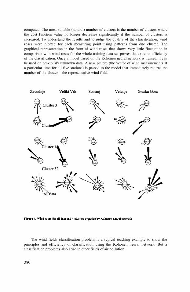
computed. The most suitable (natural) number of clusters is the number of clusters wherethe cost function value no longer decreases significantly if the number of clusters isincreased. To understand the results and to judge the quality of the classification, windroses were plotted for each measuring point using patterns from one cluster. Thegraphical representation in the form of wind roses that shows very little fluctuation incomparison with wind roses for the whole training data set proves the extreme efficiencyof the classification. Once a model based on the Kohonen neural network is trained, it canbe used on previously unknown data. A new pattern (the vector of wind measurements ata particular time for all five stations) is passed to the model that immediately returns thenumber of the cluster – the representative wind field.
The wind fields classification problem is a typical teaching example to show theprinciples and efficiency of classification using the Kohonen neural network. But aclassification problems also arise in other fields of air pollution.
380

3.2. Pattern Selection Strategies Based On The Kohonen Neural Network
Our second application of the Kohonen neural network was classification of trainingpatterns (Boznar9,8,7,10) in the process of constructing a sulphur dioxide air pollutionforecasting model. The available data base for the Sostanj basin was huge and thereforethe use of all training patterns would cause slow learning and poor results on the test dataset. The idea of the Kohonen neural network-based pattern selection strategy is to findclusters of similar training patterns and to take only representative patterns from eachcluster for the network training process. In this way the predicting neural network canlearn rare pollution events as well as frequent cases. A similar selection of patterns canalso be made manually on the basis of expert knowledge about air pollution in the studieddomain. But this “manual” method requires enormously more time and effort incomparison to the method based on the Kohonen neural network.
When using the Kohonen neural network for classification of air pollution patterns itis no longer simple to judge the quality of the classification. When the pattern – vectorconsists of ten to twenty dimensions that vary from wind to vertical temperaturedifference and concentr, it is not possible to represent the clusters graphically. Costfunctions based on standard deviations for each component can be useful. To avoid thisproblem, we simply construct the air pollution prediction model (based on the multi-layerPerceptron neural network) on the selected data from the clusters and compare thismodel’s results to the results of a model constructed with unselected data. Both patternselection strategies – the Kohonen neural network based one and the expert knowledgebased one - show significant improvement in comparison to the model trained withunselected patterns. Pattern selection strategies are also important when only mediumsized training sets (and not huge ones as in our case) are available because there is alwaysthe problem of frequent data prevailing over rare cases.
4. CONCLUSIONS
This paper is intended to show how to use efficient modern tools called artificialneural networks in the field of air pollution modelling. In our opinion these tools can beof great help in solving not only the tasks described in this paper, but also several others.We hope that the detailed explanation of cases given in the citied papers will inspire moreideas for using these tools.
5. REFERENCES
1. Rumelhart, D. E., McClelland, J. L., 1986, Parallel distributed processing 1,2, MIT Press, Cambridge, MA
2. Lawrence, J., 1991, Introduction to Neural Networks, California Scientific Software, Grass Valley
3. Kohonen, T., 1995, Self-organising maps, Springer - Verlag, Berlin
4. Hornik, K., 1991, Approximation capabilities of multilayer feedforward networks, Neural Networks,
vol.4, 251-257
5. Mlakar, P., 1997, Determination of features for air pollution forecasting models, V: ADELI, H. , ed.,
Intelligent Information Systems IIS’97, Grand Bahama Island, Bahamas, December 8-10, Proceedings.
Los Alamitos, California: IEEE Computer Society, 350-354.
381

6.
7.
8.
9.
10.
11.
12.
13.
14.
15.
16.
17.
Mlakar, P., Boznar, M., 1997, Feature determination for air pollution forecasting models. V: POWER, H.
ed., Tirabassi, T. (Ur.), Brebbia, C. A. , ed., Air pollution V: [modelling, monitoring and management].
Southampton; Boston: Computational Mechanics Publications, 577-586.
Boznar, M. Z., Mlakar, P., 2001, Artificial neural network-based environmental models, Air Pollution
Modeling and its Application XIV, ed. by Gryning and Schiermeier, Kluwer Academic / Plenum
Publishers, New York
Boznar, M., Mlakar, P., 1998, Improvement of air pollution forecasting models using feature
determination and pattern selection strategies. V: Gryning, Sven-Erik ed., Chaumerliac, Nadine. Air
pollution modeling and its application XII, (NATO challenges of modern society, vol. 22). New York;
London: Plenum Press, 725-726.
Boznar, M., 1997, Pattern selection strategies for a neural network - based short term air pollution
prediction model. V: ADELI, H. , ed., Intelligent Information Systems IIS’97, Grand Bahama Island,
Bahamas, December 8-10, 1997. Proceedings. Los Alamitos, California: IEEE Computer Society, 340-
344
Boznar, M., Mlakar, P., 1997, Pattern selection strategies for SO2 forecasting models. V: Power, H. (Ur.),
Tirabassi, T. ed., Brebbia, C. A. , Ed., Air pollution V : [modelling, monitoring and management].
Southampton; Boston: Computational Mechanics Publications, 547-556.
Boznar, M., Lesjak, M., Mlakar, P., 1993, A neural network-based method for short-term predictions of
ambient SO2 concentrations in highly polluted industrial areas of complex terrain. Atmos. environ., B
Urban atmos., vol. 27, 221-230.
Mlakar, P., Boznar, M., 1997, Perceptron neural network - based model predicts air pollution. V: ADELI,
H. , ed., Intelligent Information Systems IIS’97, Grand Bahama Island, Bahamas, December 8-10,
Proceedings. Los Alamitos, California: IEEE Computer Society, 345-349.
Mlakar, P., Boznar, M., Lesjak, M., 1994, Neural networks predict pollution. V: GRYNING, Swen-Erik
ed., MILLÁN, Millán M. , ed., Air pollution modeling and its applications (NATO challenges of modern
society, 18). New York; London: Plenum Press, 531-532
Mlakar, P., Boznar, M., 1994, Short-term air pollution prediction on the basis of artificial neural networks.
V: Baldasano, J. M. , ed., Air Pollution II. Volume 1, Computer simulation. Southampton; Boston:
Computational Mechanics Publications, 545-552.
Yi, J., Prybutok, R., 1996, A neural network model forecasting for prediction of daily maximum ozone
concentration in an industrialised urban area, Environmental Pollution 92 (3), 349-357
Boznar, M., Mlakar, P., 1995, Neural networks - a new mathematical tool for air pollution modelling. V:
Power, H. ed., Moussiopoulos, N. ed., Brebbia, C. A. , ed., Air pollution III. Volume 1, Air pollution
theory and simulation. Southampton; Boston: Computational Publications, 259-266.
Mlakar, P., Boznar, M., 1996, Analysis of winds and SO2 concentrations in complex terrain. V: Caussade,
B. ed., Power, H. ed., Brebbia, C. A. , ed., Air pollution IV : monitoring, simulation and control.
Southampton; Boston: Computational Mechanics Publications, 455-464.
382

DISCUSSION
G. COSEMANS
M. BOZNAR
You said it is difficult to predict the wind direction. Yet you are ableto predict the time series of at a monitoring site near the powerplant, while this depends mainly on the wind direction. Can youexplain this ?
Wind direction certainly is important for prediction model. Wewere not unsuccessful in wind direction forecasting, I just wanted tosay, that we had more problems with wind direction. On the otherhand the models for wind forecasting were only preliminary, but for
prediction we have done extended research. I am sure thatfurther research should bring better results also for wind directionforecasting.
383

This page intentionally left blank
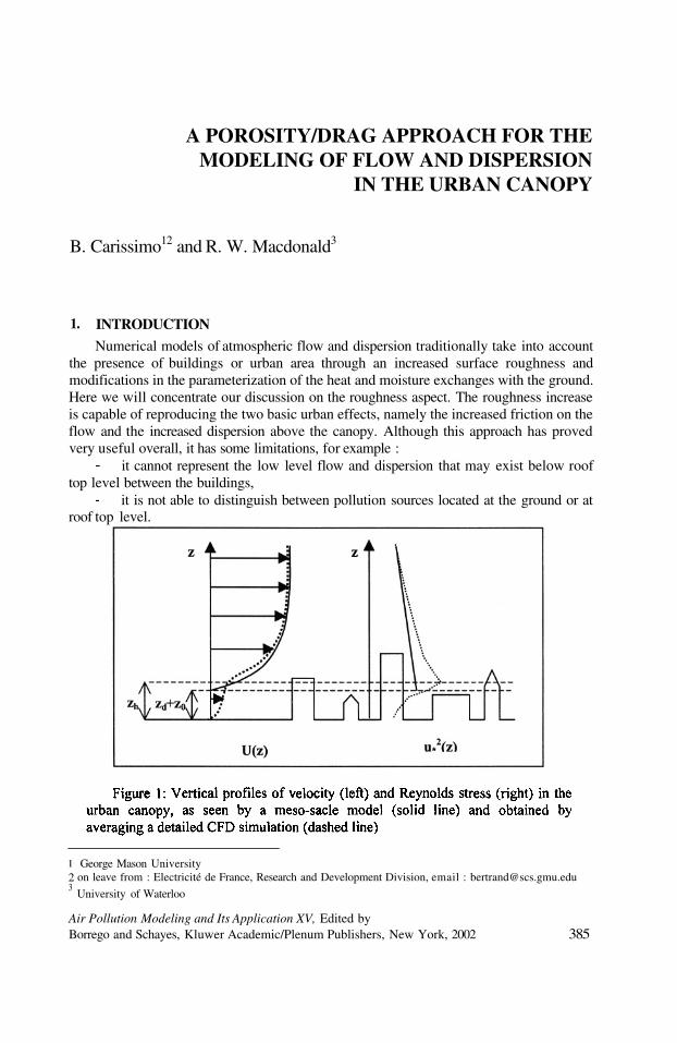
A POROSITY/DRAG APPROACH FOR THEMODELING OF FLOW AND DISPERSION
IN THE URBAN CANOPY
B. Carissimo12 and R. W. Macdonald3
1. INTRODUCTION
Numerical models of atmospheric flow and dispersion traditionally take into accountthe presence of buildings or urban area through an increased surface roughness andmodifications in the parameterization of the heat and moisture exchanges with the ground.Here we will concentrate our discussion on the roughness aspect. The roughness increaseis capable of reproducing the two basic urban effects, namely the increased friction on theflow and the increased dispersion above the canopy. Although this approach has provedvery useful overall, it has some limitations, for example :
it cannot represent the low level flow and dispersion that may exist below rooftop level between the buildings,
it is not able to distinguish between pollution sources located at the ground or atroof top level.
l
23
George Mason Universityon leave from : Electricité de France, Research and Development Division, email : [email protected]
University of Waterloo
Air Pollution Modeling and Its Application XV, Edited byBorrego and Schayes, Kluwer Academic/Plenum Publishers, New York, 2002 385

At the opposite scale, Computational Fluid Dynamics (CFD) models, have been usedto simulate the flow and dispersion around a limited number of building. Due to computerlimitations however, this simulations cannot be extended to a whole city in the nearfuture.
We are therefore in need of an intermediate approach, that can take into account theentire urban canopy but without the computer requirements of the detailed CFD, while atthe same time being compatible with the full physics of the mesoscale model.
The recent review by Brown (2000), describes the different attempts at developingsuch parameterization. The principle is to account for the area-average effect of the dragand turbulence production as additional terms in the equations of motion and theturbulence closure equations. Simpler parameterizations can be found in Hanna et al.(2001).
These new parameterizations however need to be calibrated and validated. So far,this has mainly been done crudely with available urban measurements.
In this paper we present an extended drag and porosity model, capable ofrepresenting the anisotropic effects of elongated buildings. In addition, we address theissue of calibration and validation by means of a series of high resolution, CFD, threedimensional (3D) simulations and also with physical modeling results obtained in thewater flume. Both techniques have been used to study the same geometricalconfigurations of various idealized building setup.
2. DRAG AND POROSITY MODEL DESCRIPTIONThe porosity/drag approach has been used more recently in several numerical models
(Brown, 2000, Lacser, 2001) although often in incomplete form. In our approach, thebuilding effects are taken into account by means of the following additional terms in themodel (fig. 2):
the drag force created by the buildings (modified momentum equations),the fraction of volume V occupied by solids within the flow (modified continuity
equation),the increased turbulence level (modified turbulence equations).
With thisapproach, themodel groundremains at thelevel of thetrue groundand there is noneed to takeinto account adisplacementheight due to the buildings.
Compared to earlier approaches, the drag term is formed by the product of a tensorand the velocity vector. This allows the possibility of an additional force (lift),perpendicular to the mean flow to act when the buildings are elongated (figure 3).
386

387

In figure 4, we have an example of a plume dispersing inside an idealized canopy formedby elongated buildings. This figure is a result of a high resolution numerical simulation,performed with a turbulence closure, of the geometry that will be used for the MockUrban Setting Test (MUST, Biltoft, 2001), that will be carried out in the field inSeptember 2001. The obstacle are transport containers that will be laid out in the regularpattern shown in black in the figure. In this figure, the big arrow indicates the main winddirection outside the canopy, which is at 30° off the x axis. The dashed line indicates the45° line and is much closer to the real plume axis in the canopy. In fact in this case theplume is entirely located to one side of the wind axis, a rather peculiar situation not takeninto account by simpler “urban” models. This effect cannot be reproduced by a dragmodel, in which the drag force in only proportional to the velocity vector.
The additional term in the continuity equation (fig. 2) represents the volume fractionof the canopy that is occupied by the air and not the building. This term has beenconsidered here but its relative importance on the resulting flow would require furtherstudy. Finally,, additional source terms have been implemented in the turbulenceequations. As these are even more difficult to determine than the drag values, as a firstapproach, we have taken them as zero.
3. HIGH RESOLUTION SIMULATIONS AND WATER FLUME RESULTS
As mentioned in the introduction, our objective is to use an ensemble of high-resolution numerical simulations and additional experimental results, obtained in thewater flume, to calibrate our parameterization. This section includes a description of both.
The water flume experiments are described in details in Macdonald et al. 2000 and2001. Velocities were measured using an acoustic Doppler velocimeter (SonTekMicroADV™), providing high frequency measurements of all velocity components. Thehigh frequency time series at different profile locations and different heights were thenprocessed to extract themean and turbulentvalues. Five verticalprofiles were averagedto obtain the “canopyprofile” (fig. 5).
The high-resolution numericalsimulations aredescribed in moredetails in Carissimo(2001) and Carissimoand Tehranian (2001).These simuations havebeen performed withthe MERCUREatmospheric model,developed byElectricité de Francefor atmospheric dispersion studies. It is based on a CFD code (ESTET), used for other
388
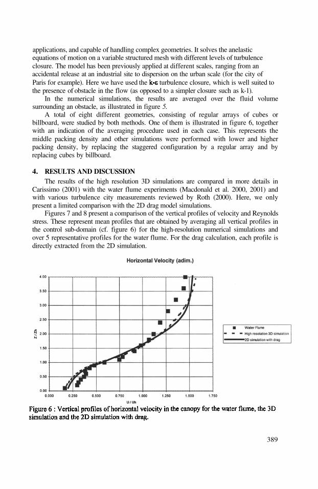
applications, and capable of handling complex geometries. It solves the anelasticequations of motion on a variable structured mesh with different levels of turbulenceclosure. The model has been previously applied at different scales, ranging from anaccidental release at an industrial site to dispersion on the urban scale (for the city ofParis for example). Here we have used the turbulence closure, which is well suited tothe presence of obstacle in the flow (as opposed to a simpler closure such as k-1).
In the numerical simulations, the results are averaged over the fluid volumesurrounding an obstacle, as illustrated in figure 5.
A total of eight different geometries, consisting of regular arrays of cubes orbillboard, were studied by both methods. One of them is illustrated in figure 6, togetherwith an indication of the averaging procedure used in each case. This represents themiddle packing density and other simulations were performed with lower and higherpacking density, by replacing the staggered configuration by a regular array and byreplacing cubes by billboard.
4. RESULTS AND DISCUSSIONThe results of the high resolution 3D simulations are compared in more details in
Carissimo (2001) with the water flume experiments (Macdonald et al. 2000, 2001) andwith various turbulence city measurements reviewed by Roth (2000). Here, we onlypresent a limited comparison with the 2D drag model simulations.
Figures 7 and 8 present a comparison of the vertical profiles of velocity and Reynoldsstress. These represent mean profiles that are obtained by averaging all vertical profiles inthe control sub-domain (cf. figure 6) for the high-resolution numerical simulations andover 5 representative profiles for the water flume. For the drag calculation, each profile isdirectly extracted from the 2D simulation.
389

The drag parameters have been optimized to obtain a velocity profile as close aspossible to that of the 3D simulations, which are also close to the profile measured in thewater flume. The value adopted for the drag coefficient is constant in height and confinedto the region z < H. Other authors have adopted a value based on the obstacle area densityA(z), which is observed to vary in height. However in our case with obstacle of the sameheight, this value is constant. This is a current limitation of our analysis that will beaddressed in future work.
The Reynolds stress profiles, which also represent the square of the friction velocityu*, are presented in figure 8. In all cases a strong maximum is found about the canopytop, with rapidly decreasing values below and more slowly decreasing values above. Inthe water flume and in the 3D simulations, the maximum is slightly above the canopy top,while it is slightly below in the drag calculation. This is a small difference that might notbe significant and the general shape of the three profiles is very similar.
The maximum value is lowest for the water flume and highest for the drag simulation.We have shown elsewhere (Carissimo, 2001) that the 3D, high resolution simulations givevalues of u* that are in line with the city observations reviewed by Roth (2000). Thisconfirms a known tendency for the laboratory scale experiments to underestimate the fullscale turbulence.
The higher values of Reynolds stress found for the drag calculation were somewhatunexpected, given that the source terms in the turbulence equations were taken as zero (cf.section 3). To explain this, we have to recall that the turbulence is produced by thevelocity shear (and other buoyancy producing terms that do not play a role here). Our
390
result therefore indicates that the shear production is overestimated by using the averagedvelocity profile, as compared to the real shear production that occurs in a fully 3D flow.We will therefore need to add “sink” terms in the turbulence equations to compensate forthis increased production. This phenomenon clearly deserves further study with morevaried geometrical configurations.
5. REFERENCES
Biltoft C., 2001 : Abbreviated test plan for Mock Urban Setting Test. DPG DocumentWDTC-TP-01-028. U.S. Army Dugway proving ground. Dugway, UT 84022-5000
Brown M.J., 2000 : Urban parameterizations for mesoscale meteorological models, inMesoscale Atmospheric Dispersion (ed. Z. Boybeyi)
Carissimo B., 2001 : Numerical simulation of flow and turbulence in simple obstaclearrays. CHARM Report, George Mason University, July 2001
Carissimo B. and S. Tehranian, 2001 : Numerical Simulations of Flow and Turbulence inSimple Obstacle Arrays. GMU Transport and dispersion modeling workshop,Fairfax VA, July 18-19, 2001
Hanna S.R., R.B. Britter, 2001 : Wind flow and vapour cloud dispersion at industrial andurban sites. to be published by AICHE,3 Park Ave, New York, NY 10016-5901
Lacser A. and T. L. Otte, 2001: Implementation of Urban Canopy Parameterization in aMesoscale Model. GMU Transport and dispersion modeling workshop, FairfaxVA, July 18-19, 2001
Macdonald R.W., S. Carter and P.R. Slawson, 2000 : Measurement of mean velocity andturbulence statistics in simple obstacle arrays at 1:200 scale. University of Waterloo.Thermal Fluids Report 2000-1, November 2000.
Macdonald R.W., S. Carter and P.R. Slawson, 2001 : Physical modeling of UrbanRoughness using arrays of regular roughness elements. (Submitted to Water, Air andSoil Pollution Focus)
Roth M., 2000 : Review of atmospheric turbulence over cities. Q.J.R. Met. Soc., 126,941-990
391

DISCUSSION
S. VARDOULAKIS
B. CARISSIMO
D. STEYN
B. CARISSIMO
S. RAFAILIDIS
B. CARISSIMO
How the shape of the velocity and Reynold stress vertical profilesmight influence the dispersion of pollutants within the Canopy(e.g. in a street canyon) ?
In our results we have considered spatially averaged profiles inthe canopy which do not show the details within a street canyon.Nevertheless, the mean concentrations in the canopy are linked tothe mean velocity profile (dilution) and to the Reynolds stressthrough the turbulent kinetic energy (diffusion).
You identify the urban canopy layer height with the maximum inReynolds stress. This is probably reasonable for a definition of thedynamical weight, but can you say something about the pollutanturban canopy layer height ?
First let me repeat that these simulations are performed in neutralconditions. Therefore we do not consider the case where unstablemotions contribute to the additional mixing of pollutants.My point here is that the maximum in Reynolds stresscorresponds to the height of the canopy, which is well defined inthis idealised case. This is found both in the laboratory and thenumerical experiments. This is also in contrast with previousauthors who found a maximum higher than the mean canopyheight in more realistic situations.
As experiment shows in the urban setting the “vertical” main
stress differs from the “horizontal” one (similar
differences exist for the component). How can theseeffects be handled in a “wall function” 2-D numerical modelwhich does not account for different parameterizations of thesedifferences in the physical features of the flow ?
The fluxes we have presented are spatial averages. Boththe numerical simulations and the laboratory experiments arebounded by vertical walls in the v direction and we have no meanmotion in that direction. On average, we therefore also expect
to be negligible although it could be locally significant.
392

H. APSIMON
B. CARISSIMO
You have illustrated the sensitivity of alignment of streets/blocksrelative to the wind direction, and diversion non of the plumewithin the canopy. How important are other effects such aschanging heights of alternate rows of blocks/buildings, inducingmore vertical fluctuations and exchange ?
This is a first step to fully understand the mean and turbulentprofiles in an idealised canopy. The next step could be, as yousay, to include for example variability in obstacle height andgeometry. We have already looked somewhat at this type ofvariability by comparing cubes and bilboard which have differenteffects on mixing in the canopy.
393

This page intentionally left blank
IMPROVED ALGORITHMS FOR ADVECTION ANDVERTICAL DIFFUSION IN AURORA
Koen De Ridder and Clemens Mensink*
1. INTRODUCTION
AURORA is an urban- to regional-scale air quality model currently underdevelopment at Vito, containing terrain, emission, chemistry, and advection-diffusionmodules. A first version, without chemistry and using simplified emissions, was brieflydescribed and used in De Ridder (2000). A recent major overhaul of AURORA’scomputer code was seized to completely re-write the advection and diffusion routines, tooptimise their functioning, and to carry out comparisons with analytical solutions. Thedescription and testing of the new advection-diffusion module, which will further bereferred to as the Eulerian Dispersion Model (EDM), constitute the focus of this paper.
The schemes dealt with here resolve (see, e.g., Jacobson, 1999)
The symbols are defined as follows: Q is the tracer mixing ratio is the airdensity is the wind vector K is the turbulent diffusion coefficient
and V is a source term The first term at the right-hand side representsadvection, and the second vertical diffusion. Horizontal diffusion is not accounted for,since it is generally small compared to artificial diffusion generated by the numericaladvection scheme.
The model grid is staggered, with scalar quantities positioned at the cell centres, andvector components at the interfaces. This corresponds to the grid structure of themesoscale model ARPS (Xue et al., 2000), which we use as meteorological driver forEDM. In the remainder of this paper, advection and diffusion are treated separately asthey are implemented using operator splitting. Both schemes are briefly described, andresults of comparisons with other schemes and with analytical solutions are shown.
* Koen De Ridder, Flemish Institute for Technological Research (Vito), Boeretang 200, B-2400 Mol, Belgium.
Air Pollution Modeling and Its Application XV, Edited byBorrego and Schayes, Kluwer Academic/Plenum Publishers, New York, 2002 395

2. ADVECTION
Among the many existing advection algorithms we selected the recent scheme byWalcek (2000). This scheme guarantees mass-conservation and monotonicity (and hencepositivity), and combines a relatively straightforward implementation with a very goodperformance, both in terms of accuracy and computational speed. In this section,Walcek’s scheme is briefly described and compared with other schemes.
The advective part of Eq. (1), in one dimension (x-direction), is given by thefollowing equation:
where u is the wind component in the x-direction. Multi-dimensional advection iscalculated by sequentially applying the one-dimensional algorithm.
Equation (2) is discretized as
where the superscript t denotes the time level, and the subscript i refers to grid position.Temporal and spatial increments are given by, respectively, and The quantitiesare used to correct density perturbations that follow from the sequential application of aone-dimensional advection algorithm in case the wind fields are not mono-dimensionallydivergence free, which would otherwise lead to spurious gradients in initially uniformconcentration fields (Clappier, 1998).
The advective fluxes at the cell interfaces are estimated using the second-order VanLeer (1977) scheme
The variable c is the Courant number (which is kept below unity tomaintain stability), and is a so-called ‘sharpening factor’, which is used to maintainconcentration gradients to the best possible extent during advection. In order to guaranteemonotonicity, is put through a number of tests and, if required, adapted. It is alsotested whether the algorithm produces new extrema in Q at in which case correctivemeasures are equally taken. For more details regarding this algorithm, including anextensive set of testing exercises, the reader is referred to the paper by Walcek (2000).
Walcek’s scheme was subjected to a one-dimensional comparative test with thefollowing advection schemes:
396
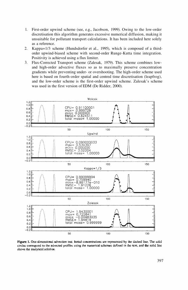
1.
2.
3.
First-order upwind scheme (see, e.g., Jacobson, 1999). Owing to the low-orderdiscretisation this algorithm generates excessive numerical diffusion, making itunsuitable for pollutant transport calculations. It has been included here solelyas a reference.Kappa=1/3 scheme (Hundsdorfer et al., 1995), which is composed of a third-order upwind-biased scheme with second-order Runge-Kutta time integration.Positivity is achieved using a flux limiter.Flux-Corrected Transport scheme (Zalesak, 1979). This scheme combines low-and high-order advective fluxes so as to maximally preserve concentrationgradients while preventing under- or overshooting. The high-order scheme usedhere is based on fourth-order spatial and centred time discretisation (leapfrog),and the low-order scheme is the first-order upwind scheme. Zalesak’s schemewas used in the first version of EDM (De Ridder, 2000).
397

The comparative test consisted of the one-dimensional advection of a parabolicinitial concentration profile with a 10 grid point-wide base, combined with a 2 point-wide hat function (Fig. 1). Advection occurs over 120 time steps with a Courant numberof c=0.8. The results, shown in Fig. 2, clearly demonstrate the excellent performance ofthe Walcek scheme. The parabolic shape is very well preserved during transport, and thesmall peak is distorted less than in the other schemes. Total mass and positivity are fullyrespected. CPU time is the lower of the schemes with exception of the first-order upwindscheme, which is no real competitor, though. Furthermore, it should be noted that theWalcek scheme requires storage of mixing ratios at one time level (at time t) only, asopposed to the Zalesak scheme using a leapfrog discretisation, which relies on two timelevels (t and meaning that the Walcek algorithm has a favourable influence oncomputer memory resources.
3. VERTICAL DIFFUSION
The diffusive part of Eq. (1) is written as
where V represents a volume source term (units of Surface and point sources canbe dealt with simply by dividing the corresponding emissions by, respectively, thevertical grid increment and the grid volume of the cell where the emission occurs. Linesources (e.g., from road traffic) are not mentioned as AURORA’s emission moduletransforms these to surface sources.
For the discretisation of Eq. (5) we partly follow Jacobson (1999), the onlydifference being that emissions are dealt with by a source term rather than by specifyingthem in the boundary conditions, yielding
indicating vertical level positions. Fluxes at the vertical cell interfaces are defined by
with the interface diffusivity taken as the average of the adjoining cells.Mixing ratios at the right-hand side of Eq. (7) are specified as a weighted average of
the mixing ratios at time levels t and using weighting factors andrespectively. In practice we use which results in the unconditionally stableCrank-Nicholson scheme. Regrouping terms results in a tridiagonal system of linearequations, which is resolved for using decomposition and forward substitution,followed by a backward substitution step (Press et al., 1992).
398

In order to test the numerical diffusion scheme, a comparison was made with ananalytical solution of Eq. (5). This was done for a one-dimensional vertical domainextending from the ground up to a mixing level height of The initialconcentration was zero everywhere, and the vertical turbulent diffusivity profile wastaken as a parabolic shape defined by
with k=0.4 von Kármán’s constant and the friction velocity, fixed at At timet=0, a surface source is activated with a strength of The numericalsimulation was performed using a time increment of 1800 s, during 20 subsequent steps.Use was made of 15 vertical levels, with depths varying from 30 m near the ground andincreasing to approximately 300 m near the domain top at 1500 m.
The analytical solution is given by
399

with t=36,000 s. The functions are Legendre polynomials, which were obtained bymeans of a recurrence relation. Equation (9) was obtained by integration of Arya’s(1999) Eq. (6.122) over the interval [0,t] and replacing the instantaneous surface sourceby a continuous one (S, units of
The result of the comparison between numerical and analytical solutions aredisplayed in Fig. 2, showing an excellent agreement. Note that the value of this exerciseis limited, since the parameterisation of turbulent transport as a diffusion process is onlya poor approximation of reality. Nonetheless, it has the merit of being a thorough checkof the validity of the numerical implementation of Eq. (5).
4. CONCLUSIONS
Modules for advection and diffusion in AURORA were re-designed, resulting in amore accurate and faster version of the Eulerian Dispersion Model (EDM). In this newversion, advection is treated by means of the recently developed algorithm by Walcek(2000), which is positive definite, mass conservative, accurate, and fast. The superiorcapacity of this scheme to preserve sharp concentration gradients was demonstrated.Vertical diffusion is treated with the well-established Crank-Nicholson scheme. Thecomparison of simulated concentration profiles with an analytical solution demonstratedthe correct functioning of those schemes.
5. REFERENCES
Arya, S.P. (1999), Air Pollution Meteorology and Dispersion. Oxford University Press, Oxford.Clappier, A. (1998), A correction method for use in multidimensional time-splitting advection algorithms:
application to two- and three-dimensional transport, Monthly Weather Review, 126, 232-242.De Ridder, K., 2000, Modelling the impact of urban/regional scale land-use patterns on atmospheric flow and
pollutant dispersion, Proceedings of the SIMPAQ-2000 Symposium, eds. Mensink et al., Vito report2000/TAP/55 (available from the author).
Hundsdorfer, W., B. Koren, M. van Loon, and J.G. Verwer (1995), A positive finite-difference advectionscheme, Journal of Computational Physics, 117, 35-46.
Jacobson, M.Z. (1999), Fundamentals of Atmospheric Modeling. Cambridge University Press, Cambridge.Press, W.H., S.A.Teukolsky, W.T. Vetterling, and B.P. Flannery (1992), Numerical Recipes in Fortran 77,
Cambridge University Press, Cambridge.Van Leer, B. (1977), Towards the ultimate conservative difference scheme. IV: a new approach to numerical
convection, Journal of Computational Physics, 23, 276-299.Walcek, C.J. (2000), Minor flux adjustment near mixing ratio extremes for simplified yet highly accurate
monotonic calculation of tracer advection, Journal of Geophysical Research, 105, 9335-9348.Xue, M., K. K. Droegemeier, and V. Wong, 2000, The Advanced Regional Prediction System (ARPS) - A
multi-scale nonhydrostatic atmospheric simulation and prediction model. Part I: Model dynamics andverification, Meteorology and Atmospheric Physics, 75, 161.
Zalesak, S.T. (1979), Fully multidimensional flux-corrected transport algorithms for fluids, Journal ofComputational Physics, 31, 335-362.
400

DISCUSSION
J. CHENEVEZ
K. DE RIDDER
A. BAKLANOV
K. DE RIDDER
A. HANSEN
K. DE RIDDER
You have compared four different advection schemes outcomes, butthe Bott advection scheme, which is one of the most used scheme inair-pollution modelling, was not included. Have you considered tocompare your results with the use of the Bott advection scheme ?
We did not ourselves include the Bott scheme in the comparisonexercise, as Walcek (2000) already describes tests comparing hisalgorithm to Bott’s and others.
You do not include the horizontal turbulent diffusion term in yourmodel and mention that it is small compared to artificial numericaldiffusion. However, for the urban scale and high-resolutionsimulations it can be not so. In this case it is necessary to control thelevel of the numerical diffusion (e.g. by horizontal grid size) toproduce realistic fields of concentrations. Did you do it ?
With the increasing accuracy of numerical advection algorithms,there is indeed concern regarding whether horizontal diffusion maybe ignored. We are currently analysing levels of physical andartificially generated diffusivities, and depending on the outcome theinclusion of horizontal diffusion in the transport equations will beconsidered.
Based on the 1-D test of the advection schemes the Walcek schemeappeared to have essentially no numerical diffusion, so that if youwant to include horizontal diffusion you must explicitly add it sincethe numerical diffusion is negligible with the Walcek-scheme.
I refer to the previous answer.
401

This page intentionally left blank

MODEL ASSESSMENT AND VERIFICATION
Chairpersons : H. ApsimonA. EbelS. Incecik
Rapporteurs : G. CosemansPh. Thunis

This page intentionally left blank
COMPARISON OF RESULTS FROM A HIGHERORDER CLOSURE DISPERSION MODEL WITH
MEASUREMENTS IN A COMPLEX TERRAIN
Babatunde J. Abiodunand Leif Enger*
1. INTRODUCTION
Air quality models are used as the most powerful and the only scientificallyrelevant tools for identifying effective strategies to improving air quality. They are veryuseful in getting air-quality data, particularly in the areas lacking observational data.Higher order closure dispersion models have been successfully used to simulate pollutantdynamics over many urban area and complex terrain (e.g. Enger and Koracin,1995Abiodun et.al., 2001).
This paper presents a higher-order closure dispersion (HOCD) model, suitable fordispersion in urban area and complex terrain. The model is used to reproduced a tracerdispersion experiment in a complex terrain that was performed during an extensive fieldprogram, MOHAVE (Measurements Of Haze And Visibility Experiment) (see Green,1999; Pitchford et al., 1999). A brief description of the model is presented in the nextsection. Section 3 discusses the project MOHAVE and the model initialization. Modelresults, in comparison to measurement, are discussed in section 4.
2. MODEL DESCRIPTION
The present model is an Eulerian diffusion model, which starts from the masscontinuity equation
* Babatunde J. Abiodun, Department of Meteorology, Federal University of Technology, P.M.B.704, Akure, Nigeria. Leif Enger, Department of Earth Sciences, Uppsala University, Villavägen16, 752 36 Uppsala, Sweden
Air Pollution Modeling and Its Application XV, Edited byBorrego and Schayes, Kluwer Academic/Plenum Publishers, New York, 2002 405

The corresponding equations for the turbulence fluxes, if we neglect molecularterms and the effect of Coriolis force on the covariance, are
The equation for the covariance, is
The pressure covariance terms in equation (2) are parameterised according toEnger (1986) as
where is a constant, and is a master turbulent length scale.The vertical transport term is parameterized using a gradient diffusion
approximation according to Donalson (1973) and Mellor (1973). The moleculardestruction term D is parameterized according to Lumely (1975) as
The values for the constants, and are 0.3465 and 0.144 respectively. Theformulations of the master length scale, can be obtained in Enger (1990). A finite-difference numerical method is used to solve the set of the model equations. The modeluses an expanding telescoping grid mesh with its origin at the source. This means that weget more dense grid mesh near the source where the plume is narrower than furtherdownstream. The prognostic equations in the dispersion model are solved by using a thirdorder advection scheme described in Enger and Grisogono (1997). The diffusion issolved with a semi-implicit scheme with weight 0.75 on the future time step. TheArakawa staggered C-grid is used for the model structure. The following boundaryconditions are applied at the top of the model
406

and the following at the surface
3. MOHAVE PROJECT AND MODEL INITIALIZATION
MOHAVE project was conducted in the southwestern United States (see Figure 1)and included meteorological, chemical and visibility measurements at several stations.Upper-air observations were made at several sites using radiosondes, wind profilers and aradio acoustic sounding system (RASS). The main goal of the project was to assess theeffects of the Mohave Power Plant (MOPP), a large coal-fired power plant in ColoradoRiver Valley in southern Nevada, circa 120 km to the south-southeast of Las Vegas, uponvisibility in the southwestern United States, in particular at Grand Canyon national park(Green, 1999). During the experiment, PTF ortho-perfluodimethylcyclohexane (oPDCH)was released continuously for 50 days in summer from the MPP. Forty-five percent of theoPDCH consists of the isomer ortho-cis (oc)PDCH, which was measured at the receptorsites. The tracers are inert, non-depositing, and non-toxic chemicals. The stack height ofthe power plant is 150m. The effective source height is calculated to be about 300m, andfor the present study we use 300m in dispersion model. The average release rate ofoPDCH for the period is about 0.042g/s. Details of the experiment and measurement canbe obtained in Green (1999) and Isakov (1998). The measurement used for modelcomparison in the present study is obtained from Isakov (1998), but converted fromfemtoliters per liter (fl/L) to microgram per unit volume
407

Dynamic flow fields and the turbulence over the study area for the period (5/8/92– 14/8/92) have been simulated with the MIUU (Meteorological Institute UppsalaUniversity) mesoscale model and reported in Morh. et.al 2001. The study shows that thesimulated fields compare fairly well with the observations. For the present study, thesimulated results for the first four days, which are stored at 1-hour interval, wereinterpolated to five minutes interval and used in the dispersion model. Figure 2(a) and2(b) show the interpolated horizontal wind vector at 100m AGL from MIUU modeldomain to the dispersion model grid point at 1200 MST (5/8/92) and 1700 MST (6/8/92).Note that the wind vectors at every fifth grid point are plotted. The domain terrain and thereceptor sites are shown in the background. The results generally show southerly andsouthwesterly flows over the area. The southerly flow is stronger along the Coloradovalley and follows the bending shape of the valley. Effects of the anabatic and katabaticwinds along the mountain slope, due to horizontal pressure gradient created by thetemperature differences, are visible on the simulated flow at 1200 and 7000 MSTrespectively, especially around SPMO and the adjacent mountains.
408
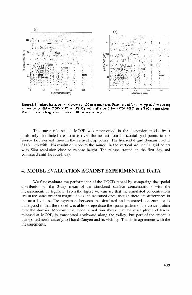
The tracer released at MOPP was represented in the dispersion model by auniformly distributed area source over the nearest four horizontal grid points to thesource location and three in the vertical grip points. The horizontal grid domain used is81x81 km with 1km resolution close to the source. In the vertical we use 31 grid pointswith 50m resolution close to release height. The release started on the first day andcontinued until the fourth day.
4. MODEL EVALUATION AGAINST EXPERIMENTAL DATA
We first evaluate the performance of the HOCD model by comparing the spatialdistribution of the 3-day mean of the simulated surface concentrations with themeasurements in figure 3. From the figure we can see that the simulated concentrationsare in the same order of magnitude as the measured ones, though there are differences inthe actual values. The agreement between the simulated and measured concentration isquite good in that the model was able to reproduce the spatial pattern of the concentrationover the domain. Moreover the model simulation shows that the main plume of tracer,released at MOPP, is transported northward along the valley, but part of the tracer istransported north-easterly to Grand Canyon and its vicinity. This is in agreement with themeasurements.
409
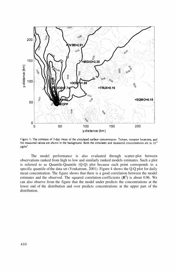
The model performance is also evaluated through scatter-plot betweenobservations ranked from high to low and similarly ranked models estimates. Such a plotis referred to as Quantile-Quantile (Q-Q) plot because each point corresponds to aspecific quantile of the data set (Venkatram, 2001). Figure 4 shows the Q-Q plot for dailymean concentration. The figure shows that there is a good correlation between the modelestimates and the observed. The squared correlation coefficients is about 0.96. Wecan also observe from the figure that the model under predicts the concentrations at thelower end of the distribution and over predicts concentrations at the upper part of thedistribution.
410
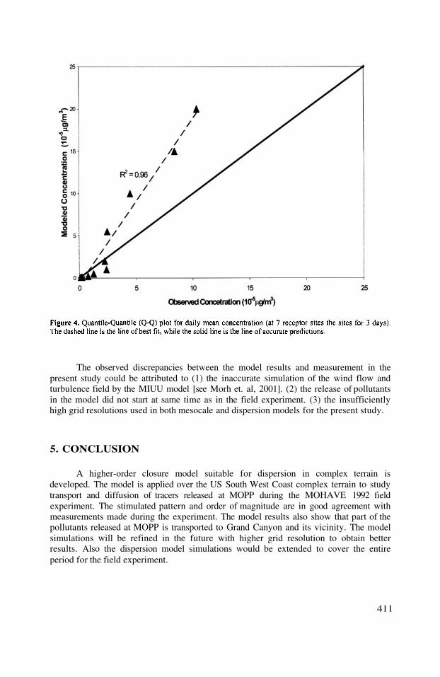
The observed discrepancies between the model results and measurement in thepresent study could be attributed to (1) the inaccurate simulation of the wind flow andturbulence field by the MIUU model [see Morh et. al, 2001]. (2) the release of pollutantsin the model did not start at same time as in the field experiment. (3) the insufficientlyhigh grid resolutions used in both mesocale and dispersion models for the present study.
5. CONCLUSION
A higher-order closure model suitable for dispersion in complex terrain isdeveloped. The model is applied over the US South West Coast complex terrain to studytransport and diffusion of tracers released at MOPP during the MOHAVE 1992 fieldexperiment. The stimulated pattern and order of magnitude are in good agreement withmeasurements made during the experiment. The model results also show that part of thepollutants released at MOPP is transported to Grand Canyon and its vicinity. The modelsimulations will be refined in the future with higher grid resolution to obtain betterresults. Also the dispersion model simulations would be extended to cover the entireperiod for the field experiment.
411
6. ACKNOWLEDGEMENTS
This study was sponsored by the Office of Naval Research (contract N00014-98-1-0557), by the Swedish National Research Council (contract G-AA/GU 12471-300), andby the International Science Program, Uppsala University (project NIG02).
7. REFERENCES
Abiodun B.J., L. Enger and M. Morh (2001) ‘Modelling of atmospheric pollutants dispersion in complexterrain – part II: Development and validation of a Higher-Order Closure Dispersion model’, Proceedingsof Int. Conference on Hamonisation within Atmospheric Dispersion Modelling for RegulatoryPurposes, Belgirate, Italy. 355-359.
Donaldson, C. du P. (1973), ‘Construction of a dynamic model of the production of atmosphere turbulence andthe dispersal of atmospheric pollutants’, In Workshop on Micrometeorology (edited by Haugen D.A.),American Meteorological Society publication, pp. 392.
Enger, L. (1986), ‘A higher order closure model applied to dispersion in a convective PBL’, Atmos. Environ.,Vol. 20, pp. 879-894.
Enger, L. (1990), ‘Simulation of dispersion in moderately complex terrain-Part B. The higher order closuredispersion model’, Atmos. Environ., Vol. 24, pp. 2447-2455.
Enger, L. and B. Grisogono (1997), ‘The response of bora-type flow to sea surface temperature’, Q. J. R.Meteorol. Soc., Vol. 124, pp. 1227-1244.
Enger, L. and D. Koracin (1995), ‘Simulations of dispersion in complex terrain using a Higher-Order ClosureModel’, Atmos. Environ., Vol. 29, No. 18, pp. 2449-2465.
Green, M.C., (1999), ‘The Project MOHAVE tracer study: Study design, data quality, and overview of results’,Atmos. Environ., Vol. 33, pp. 1955-1968.
Isakov, V. (1998), ‘Evaluation of Atmospheric and Dispersion models in complex terrain by using tracermeasurements’, Ph.D. Thesis, 119 pp. [Available from Division of Atmospheric Sciences, DesertResearch Institute, 2215 Raggio Parkway , Reno, NV 89512]
Lumley, J.L. (1975), Prediction methods for turbulent flows, VKI-LS 76, Rhode-St-Genese, Belgium.Mellor, G. (1973), ‘Analytical prediction of the properties of stratified planetary surface layers’, J. Atmos. Sci.,
Vol. 30, pp. 1061-1069.Morh M, L. Enger and B.J. Abiodun (2001): ‘Modelling of atmospheric pollutant dispersion in complex terrain
– Part I: Development validation and comparison of Higher Order Closure Mesoscale models’,Proceedings of Int. Conference on Hamonisation within Atmospheric Dispersion Modelling forRegulatory Purposes, Belgirate, Italy. 350-354.
Venkatram, A. (2001 ) ‘An Approach to developing air quality models for regulatory applications’, Proceedingsof Int. Conference on Hamonisation within Atmospheric Dispersion Modelling for RegulatoryPurposes, Belgirate, Italy. 37-41
Yamada, T. (1985), ‘Numerical simulations of valley ventilation and pollutant transport. Proc. Symposium onTurbulence and Diffusion with Boulder, Colorado. Amer. Meteor. Soc. 312-314.
412

DISCUSSION
A. HANSEN
B.J. ABIODUN
Because of the overprediction of tracer concentrations in the farfield, it appears that your model is creating mass. Is this possible ?
A closer look at figure 4 actually suggests that the modeloverpredicts trace concentration close to the source, rather than inthe far field as you said. The reason for this is that the MOHAVEpoint source is introduced in the model as an area source, due to thenature of the model.Moreover we cannot also conclude that the model underpredictstracer concentration in the far field, because a look at figure 3reveals that downwind, the model underpredicts to the eastern sideand overpredicts to the western side. This suggests a drift of themodel plume more to the west than the measurements.Lastly the mass conservation of the model had been tested in theprevious experiments. We found that the model neither create nordestroy mass.
H. APSIMON How sensitive are your model estimates in the MOHAVEexperiment to the initial dispersion ? If this was slightly enhanced itwould probably extend the spread of the plume and improveagreement with observations ?
B.J. ABIODUN We did not investigate the sensitivity of the model estimates in theMOHAVE experiment to the initial dispersion. We will do this inour next validation experiment.
413

This page intentionally left blank

PARAMETERISATION OF SBL HEIGHT INATMOSPHERIC POLLUTION MODELS
Alexander Baklanov*
1. INTRODUCTION
Models of atmospheric transport of pollutants demand knowledge of the structure of theatmospheric boundary layer (ABL). A very important characteristic for such models,especially for stably stratified boundary layers (SBL), is the height of the atmosphericboundary layer, h. The upper boundary of the SBL often plays a role of a lid preventingpollutants to escape the SBL, so it is commonly called a mixing height (MH). The mixingheight in the dispersion models can practically be determined by two basic ways. It can beobtained from profile measurements, either in-situ or by remote sounding. The otherpossibility is to use parameterisations with only a few measured parameters as input or tosubstitute output from numerical weather prediction models for observed parameters.
The working group 2 ‘Mixing Height Determination for Dispersion Modelling’ ofthe EU COST Action 710 in the final project report (Seibert et al., 1998) has presented avery detailed analysis of the existing methods and approaches for the MH determinationand, as a recommendation for future research, has stated that there is a general need formore research on SBL. Formulae for the mechanical mixing height, especially those basedon Richardson numbers, should be tested on a number of data sets. The validity of the MHconcepts originating from boundary layer studies to describe the pollutant dispersionshould be studied, especially with respect to the effects of intermittent turbulence and ofwaves in outer SBL. Especially critical are the cases with long lived and very shallowSBLs of northern or coastal regions (Zilitinkevich et al., 2001a). In the thoroughly stablestratification (without the residual layer), typical for high latitudes and also for coastalzones, the vertical wave propagation is not blocked. As a result, the stable-boundary-layerturbulence becomes essentially non-local, and the traditional local theory predicts aninsufficient turbulence mixing.
* Alexander Baklanov, Danish Meteorological Institute (DMI), Lyngbyvej 100 DK-2100 Copenhagen Denmark
Air Pollution Modeling and Its Application XV, Edited byBorrego and Schayes, Kluwer Academic/Plenum Publishers, New York, 2002 415
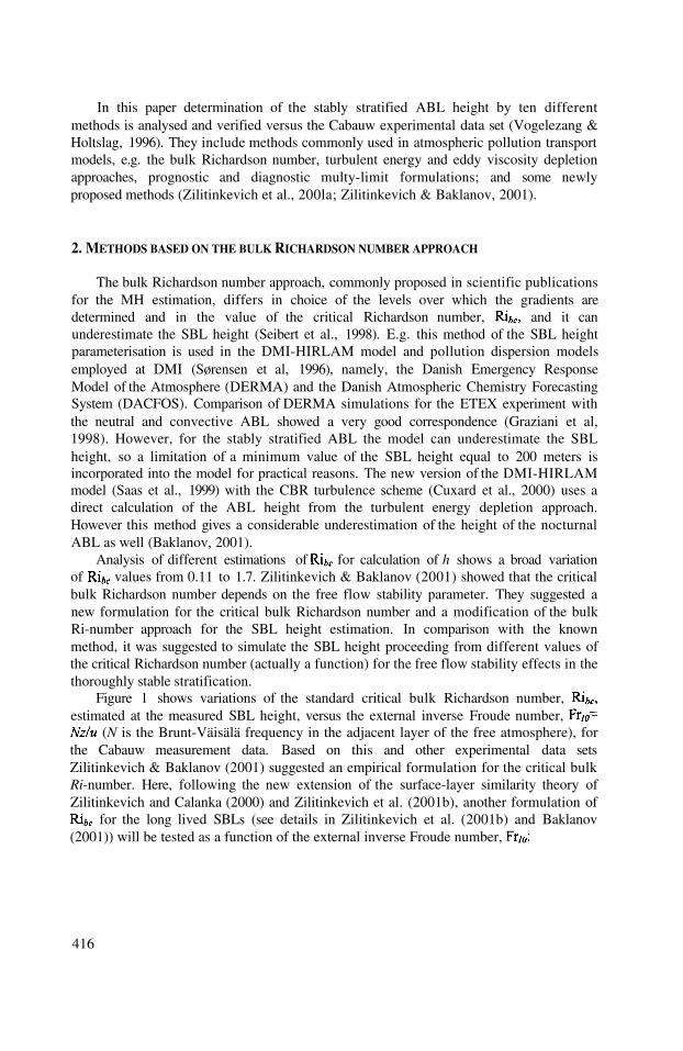
In this paper determination of the stably stratified ABL height by ten differentmethods is analysed and verified versus the Cabauw experimental data set (Vogelezang &Holtslag, 1996). They include methods commonly used in atmospheric pollution transportmodels, e.g. the bulk Richardson number, turbulent energy and eddy viscosity depletionapproaches, prognostic and diagnostic multy-limit formulations; and some newlyproposed methods (Zilitinkevich et al., 200la; Zilitinkevich & Baklanov, 2001).
2. METHODS BASED ON THE BULK RICHARDSON NUMBER APPROACH
The bulk Richardson number approach, commonly proposed in scientific publicationsfor the MH estimation, differs in choice of the levels over which the gradients aredetermined and in the value of the critical Richardson number, and it canunderestimate the SBL height (Seibert et al., 1998). E.g. this method of the SBL heightparameterisation is used in the DMI-HIRLAM model and pollution dispersion modelsemployed at DMI (Sørensen et al, 1996), namely, the Danish Emergency ResponseModel of the Atmosphere (DERMA) and the Danish Atmospheric Chemistry ForecastingSystem (DACFOS). Comparison of DERMA simulations for the ETEX experiment withthe neutral and convective ABL showed a very good correspondence (Graziani et al,1998). However, for the stably stratified ABL the model can underestimate the SBLheight, so a limitation of a minimum value of the SBL height equal to 200 meters isincorporated into the model for practical reasons. The new version of the DMI-HIRLAMmodel (Saas et al., 1999) with the CBR turbulence scheme (Cuxard et al., 2000) uses adirect calculation of the ABL height from the turbulent energy depletion approach.However this method gives a considerable underestimation of the height of the nocturnalABL as well (Baklanov, 2001).
Analysis of different estimations of for calculation of h shows a broad variationof values from 0.11 to 1.7. Zilitinkevich & Baklanov (2001) showed that the criticalbulk Richardson number depends on the free flow stability parameter. They suggested anew formulation for the critical bulk Richardson number and a modification of the bulkRi-number approach for the SBL height estimation. In comparison with the knownmethod, it was suggested to simulate the SBL height proceeding from different values ofthe critical Richardson number (actually a function) for the free flow stability effects in thethoroughly stable stratification.
Figure 1 shows variations of the standard critical bulk Richardson number,estimated at the measured SBL height, versus the external inverse Froude number,
(N is the Brunt-Väisälä frequency in the adjacent layer of the free atmosphere), forthe Cabauw measurement data. Based on this and other experimental data setsZilitinkevich & Baklanov (2001) suggested an empirical formulation for the critical bulkRi-number. Here, following the new extension of the surface-layer similarity theory ofZilitinkevich and Calanka (2000) and Zilitinkevich et al. (2001b), another formulation of
for the long lived SBLs (see details in Zilitinkevich et al. (2001b) and Baklanov(2001)) will be tested as a function of the external inverse Froude number,
416
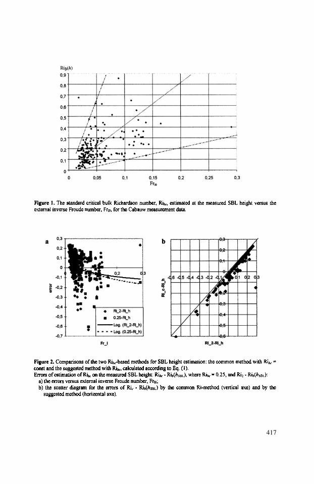
417
where: are the von Karman constants for momentum and heat,
correspondingly; and are two parameters dependent on
the height and roughness lengths; are empirical constants (according toZilitinkevich et al. (2001a)
Let’s compare two -based methods for the SBL height estimation: the commonmethod (e.g., Mahrt, 1981) with and the suggested method withcalculated according to Eq. (1). Figure 2 shows errors of estimation on the measuredSBL height: where and In Figure 2a, the errorsare presented vs. external inverse Froude number, for the Cabauw data. Figure 2bpresents a scatter diagram for the errors of by the common Ri-method(vertical axis) and errors by the suggested method (horizontal axis). As seen, both graphsin Figure 2 show that the proposed approach, Eq. (1), considerably improves the methodof the SBL height estimation. The bias of the estimated critical value of on the top ofthe SBL height is 0.054 and 0.006 for the standard approach and thesuggested modified method, Eq. (1), respectively.
However, it is necessary to note, that the discussed approach needs an additionalimprovement and verification vs. measurement data and testing with different models.
3. FORMULATIONS BASED ON EQUATION OF TKE BUDGET
Many different methods, commonly used in dispersion models for the MH estimation,are based on analysis of the turbulent kinetic energy budget and different length scales(e.g., Rossby & Montgomery, 1935; Zilitinkevich, 1972; Pollard et al., 1973; Arya, 1981;Mahrt et al., 1982; Nieuwstadt, 1984). Zilitinkevich and Mironov (1996) (henceforth ZM)summarised the SBL height parameterisation results from a number of earlier studies. Themulti-limit diagnostic formulation of ZM became widespread among air pollutionmodellers (see e.g. Robertson et al., 1996; Brandt, 1998; Linqvist, 1998; Anquetin et al.,1999; Baklanov, 1999; Langer et al. 1999) during the last years. However, some authors(e.g. Zilitinkevich & Baklanov, 2001) pointed out an underestimation of SBL height bythe formulation and, the constants had to be verified vs. experimental data. It was shownthere that re-estimation of the constants and modification by incorporating the meanvertical velocity at the SBL top gave a better correlation with the measurements.However, further analysis given by Zilitinkevich et al. (2001a) shows that two limits in theZM formulation: for the SBL dominantly affected by the surface buoyancy flux(Kitaigorodskii, 1960), and for the SBL dominantly affected by the free-flow
static stability (Kitaigorodskii and Joffre, 1988), are inappropriate for the Ekman layer.Recent theoretical studies of non-local turbulence in the thoroughly stable stratification(Zilitinkevich & Calanca, 2000; Zilitinkevich, 2001; Zilitinkevich et al., 2001a) deepenunderstanding of its nature and provide an improved parameterisation of turbulence fluxesand PBL structure, which will be useful for parameterisation of the long-lived SBL height.
418

So, an alternative for ZM formulation for SBL height of the Ekman layer, includingthe effects of the free flow stability was proposed in Zilitinkevich et al. (2001a).According to that, extended surface-layer similarity theory taking into account possibledistant interactions in the thoroughly stable stratification and interpolating with the knownformulation of the neutrally stratified ABL yields new diagnostic (see below Eq. [8]) andprognostic formulations. The proposed method covers a broad spectrum of cases: both thenocturnal SBLs, typical for the middle latitudes, and the strongly stratified long-livedSBLs.
4. COMPARATIVE ANALYSIS OF DIFFERENT FORMULATIONS FOR SBL HEIGHT
Zilitinkevich et al. (2001a) and Zilitinkevich & Baklanov (2001) showed that the newmodified formulation, Eq. [8], is in a reasonably good agreement with the experimentaldata and is better than the ZM multi-limit formulation, Eq. [7]. However, it is alsonecessary to give a comparative analysis of the discussed formulations with other differentformulations for SBL height. Let’s consider the comparative analysis with the Cabauwdata set. The following eight formulations, commonly cited in the scientific literature (seee.g. Lena & Desiato (1999); Zilitinkevich & Baklanov (2001)), were used for theverification:
[1] after Zilitinkevich (1972) 1:
[2] Nieuwstadt (1984):
[3] Arya (1981):
[4] Mahrt et al. (1982):
[5] Benkley & Schulman (1979):
[6] Nieuwstadt (1984):
[7] Zilitinkevich and Mironov (1996):
[8] Zilitinkevich et al. (2001a):
1Version modified by Aria (1981) with re-estimated constants.
419

The bulk Richardson number approach was not used in the simulations, because it wasalready analysed for different variants of the approach (Vogelezang & Holtslag, 1996) forthe same data set. However, as it was shown in Chapt. 2, the modified bulk Richardsonnumber method, Eq. (1), gives better results than the common bulk Richardson numberapproach.
420
Results of the simulations and verification of the SBL height parameterisations [1] -[8] versus the Cabauw data are presented in Figure 3 and analysed in Zilitinkevich &Baklanov (2001). As it is seen, the new formulation of Zilitinkevich et al. (2001a), Eq.[8], is best supported by measurement data compared to the other seven formulations.
5. DISCUSSION AND CONCLUSION
Determination of the stably stratified ABL height by ten different methods is analysedand verified versus the Cabauw experimental data set (Vogelezang & Holtslag, 1996). Theverified metods include methods commonly used in atmospheric pollution transportmodels, e.g. the bulk Richardson number, turbulent energy and eddy viscosity depletionapproaches, the multy-limit formulations; and some newly proposed methods(Zilitinkevich et al., 2001a; Zilitinkevich & Baklanov, 2001).
It was shown that the critical bulk Richardson number, is not a constant anddepends on the free flow stability, including the external inverse Froude number,
Following Zilitinkevich et al. (2001b) and Zilitinkevich & Baklanov (2001) the newformulation (1) for the critical bulk Richardson number, and a modification of thebulk Ri-number approach for the SBL height estimation are discussed and verified. Incomparison with the known method, it is suggested to simulate the SBL height proceedingfrom different values of the critical Richardson number (actually a function (1)) for thefree flow stability effects in the thoroughly stable stratification. Comparison withmeasurement data showed that the proposed approach, Eq. (1), considerably improves theRi-method of the SBL height estimation. However, it is necessary to note, that thediscussed approach needs an additional improvement, verification and testing withdifferent models.
It is shown that the last formulation for the SBL height, Eq. [8] (Zilitinkevich et al.(2001a), gives a better correspondence with the experimental data. The suggestedparameterisations the SBL height will be tested in the DMI-HIRLAM model and pollutiondispersion models employed at DMI, namely, the DERMA and DACFOS.
ACKNOWLEDGEMENTS
The author is extremely grateful to Sergej Zilitinkevich (Uppsala University) whohave initiated this study and suggested many perfect ideas. Thanks to Bert Holtslag andDaan Vogelezang (KNMI) for providing the Cabauw data, Alix Rasmussen, Jens HavskovSørensen and Niels Woetmann Nielsen (DMI) for their helpful advices and AlexanderMahura for comments on the manuscript. This work was partly supported by the DanishForskningsstyrelsen – START-project No. 44.2207.4422.
REFERENCES
Anquetin, S., Chollet, J. P., Coppalle, A., Mestayer, P. G., Sini, J. F., 1999, The Urban Atmosphere Model:SUBMESO, Proceedings of EUROTRAC Symposium ‘98, P.M Sorrel & P. Borrel, Edits., WITpress.
421
Arya, S.P.S., 1981, Parameterizing the height of the stable atmospheric boundary layer, J. Appl. Meteorol. 20,1192-1202.
Baklanov, A., 1999, Modelling of episodes of atmospheric transport and deposition: Hypothetical nuclearaccidents in North-West Russia, in: Nuclear Risks, Environmental and Development Cooperation in theNorth of Europe. CERUM, University of Umea, Sweden, pp. 65-80.
Baklanov, A., 2001, Parameterisation of the SBL height in atmospheric models. Presentation on the Workshop onStable Boundary Layers, Uppsala University, Sweden, 12-14 September 2000 (as DMI Report).
Benkley, C.W. and Schulman, L.L., 1979, Estimating mixing depths from historical meteorological data, J. Appl.Meteorol. 18, 772-780.
Brant, J., 1998, Modelling transport, dispersion and deposition of passive tracers from accidental releases. PhDthesis. RISO-NERI, Denmark, August 1998.
Cuxard, J., Bougeault, P. and Redelsperger, J.-R., 2000, A turbulence scheme allowing for mesoscale and large-eddy simulations. Quart. J. Roy. Meteor. Soc., 126, 1-30.
Graziani, G., Klug, W., and Mosca, S., 1998, Real-Time Long-Range Dispersion Model Evaluation of the ETEXfirst Release, Office for Official Pub. of the European Communities, Luxembourg, EUR 17754 EN.
Kitaigorodskii, S. A., 1960, On the computation of the thickness of the wind-mixing layer in the ocean, Izvestiya, Ser.Geophys., 3, 425-431.
Kitaigorodskii, S. A., and Joffre, S. M., 1988, In search of simple scaling for the heights of the stratifiedatmospheric boundary layer, Tellus, 40A, 419-43.
Lena, F. and Desiato, F., 1999, Intercomparison of nocturnal mixing height estimate methods for urban airpollution modelling. Atmospheric Environment, 33(15): 2385-2393.
Linqvist, J., 1999, En stokastik partikelmodell i ett icke-metriskt koordinatsystem. FOA report. FOA NBC-defence, Umeå, Sweden. 46 p. (in Swedish).
Mahrt, L., 1981, Modelling the depth of the stable boundary layer, Boundary-Layer Meteoriol., 21, 3-19.Mahrt, L., Andre, J.C., Heald, R.C., 1982, On the depth of the nocturnal boundary layer. J. Appl. Meteorol. 21,
90-92.Nieuwstadt, F.T.M., 1984, The turbulent structure of the stable, nocturnal boundary layer, J. Atmos. Sci. 41, 2202-
2216.Pollard, R. T., Rhines, P. B., and Thompson, R. O. R. Y., 1973, The deepening of the wind-mixed layer, Geophys.
Fluid Dyn., 3, 381-404Robertson, L., Langner, J. and Engardt, M., 1996, MATCH - Meso-scale Atmospheric Transport and Chemistry
modelling system. Basic transport model description and control experiments with SMHI RMK No70, Norrkoping, Sweden
Rossby, C. G., and Montgomery, R. B., 1935, The layer of frictional influence in wind and ocean currents, Pap.Phys. Oceanogr. Meteorol., 3, No.3, 1-101
Saas, B.H., Nielsen, N.W., Jørgensen, J.U. and Amstrup, B., 1999, The operational DMI-HIRLAM system. DMItechnical report #99-21.
Seibert, P., Beyrich, F., Gryning, S.-E., Joffre, S., Rasmussen, A. and Tercier, Ph., 1998, Mixing HeightDetermination for Dispersion Modelling. Report of Working group 2, in: COST Action 710. Preprocessing ofMeteorological Data for Dispersion Modelling. May 1997.
Sørensen, J.H., Rasmussen, A. and Svensmark, H., 1996, Forecast of Atmospheric Boundary-Layer Height forETEX Real-time Dispersion Modelling, Phys. Chem. Earth, 21, No. 5-6, pp. 435-439.
Vogelezang, D.H.P. and Holtslag, A.A.M., 1996, Evolution and model impacts of the alternative boundary layerformulations. Boundary-Layer Meteor., 81, 245-269.
Zilitinkevich, S. S., 1972, On the determination of the height of the Ekman boundary layer, Boundary-LayerMeteorol., 3, 141-145.
Zilitinkevich, S. S., 2001, Third-order transport due to internal waves and non-local turbulence in the stablystratified surface layer. Submitted to Quart. J. Roy. Meteorol. Soc.
Zilitinkevich, S. and Baklanov, A., 2001, Calculation of the height of stable boundary layers in operational models.Submitted to Boundary-Layer Meteorology.
Zilitinkevich, S., Baklanov, A., Rost, J., Smedman, A.-S., Lykosov, V. and Calanca, P., 2001a, Diagnostic andprognostic equations for the depth of the stably stratified Ekman boundary layer. Accepted to Quart. J. Roy.Meteorol. Soc.
Zilitinkevich, S., and Calanca, P., 2000, An extended similarity-theory formulation for the stably stratifiedatmospheric surface layer. Quart. J. Roy. Meteorol. Soc., 126, no. 566, pp. 1970-85.
Zilitinkevich, S., and Mironov, D. V., 1996, A multi-limit formulation for the equilibrium depth of a stablystratified boundary layer, Boundary-Layer Meteorol., 81, 325-351.
422

Zilitinkevich, S. S., Perov, V. and King, J., 2001b, Near-surface turbulent fluxes in stable stratification: calculationtechniques for use in general circulation models, Submitted to Quart. J. Roy. Meteorol. Soc.
423

DISCUSSION
S.E. GRYNING Over the last 20 years, more than 15 parameterizations of the heightof the SBL has been suggested, all based on the four parameters
N and f. Comparison with data is generally poor. Do you
consider that a general parameterization of the height of the SBL ispossible ? I suggest to consider for future parameterization of theSBL height, a partitioning of the SBL into a weakly stable part
(where increases with stability, and M-O theory is
applicable), and a very stable part (where decreases with
stability) where new scaling parameters has to be used likelyincluding the effect of breaking waves.
A. BAKLANOV Actually, most of the parameterisations used only three of theparameters mentioned above. The first attempt to include all fourparameters was done by Zilitinkevich and Mironov (1996).However, it was done by asymptotic incorporation of all knownlimits, and two of them were not valid for the Ekman layer.Your suggestion is correct. Actually, this principle to distinguish intotwo regimes of SBL was realised in the newest parameterisations ofthe height of the SBL, suggested by Zilitinkevich, Baklanov, Rost,Smedman, Lykosov and Calanca, (Quarterly Journal of the RoyalMeteorological Society, 2001, Vol. 127, No. 578) and byZilitinkevich and Baklanov (2001, Boundary-Layer Meteorology,accepted). The formula [8], which shows the relatively bestcorrespondence with the measurements, includes the non-local effectof breaking waves for the very stable (long-lived) SBL and reducesto the well known formulation of Zilitinkevich (1972) for the weaklystable (flux-dominated) SBL, when .M-O theory is valid.
424
EVALUATION OF MIXING HEIGHTPARAMETERIZATIONS FOR AIR
POLLUTION MODELS
Laurent Delobbe, Olivier Brasseur, Jan Matthijsen, Clemens Mensink,Ferd J. Sauter, Guy Schayes, and Daan P.J. Swart*
1. INTRODUCTION
The mixing height (MH) is a fundamental parameter in many air pollution models.Its practical determination is often based on simple parameterizations, which only need afew input meteorological parameters. For validation purpose, it is useful to compare theresults of these parameterizations with more sophisticated methods and withmeasurements
In this study, we evaluate the mixing height parameterization used in thephotochemical transport model EUROS, developed at RIVM (van Loon, 1996). The MHevolution at Bilthoven (The Netherlands) for August 1997 calculated by EUROS hasbeen compared with three other estimates: (1) from the ECMWF vertical profiles using aRichardson number method, (2) from the LIDAR measurements at RIVM (Bilthoven),(3) from a more sophisticated MH parameterization implemented in the EUROS model.
2. MIXING HEIGHT DETERMINATION
2.1 Standard Euros Formulation
In EUROS, the MH (H) is calculated from the friction velocity (u*), the Monin-Obukhov length (L) and the surface sensible heat flux using simpleparameterizations found in the literature (Nieuwstadt, 1981; Holtslag andWestrhenen,1989; Tennekes, 1973). Three stability cases are considered. In stable,
* Laurent Delobbe and Clemens Mensink, Flemish Institute for Technological Research (Vito), Boeretang 200,B-2400 Mol, Belgium. Olivier Brasseur and Guy Schayes, UCL, Institut d’Astronomie et de Géophysique G.Lemaître, Chemin du Cyclotron 2, B-1348 Louvain-la-Neuve, Belgium. Jan Matthijsen, Ferd Sauter, and DaanSwart, RIVM, Air Research Laboratory, PB1, 3720 BA Bilthoven, The Netherlands.
Air Pollution Modeling and Its Application XV, Edited byBorrego and Schayes, Kluwer Academic/Plenum Publishers, New York, 2002 425

neutral and unstable conditions, the MH is formulated following (1), (2) and (3),respectively.
In these expressions is the potential temperature gradient above the convectiveboundary layer and f is the coriolis parameter. The surface meteorological parameters u*,L, and are calculated using a software library developed at KNMI (Beljaars andHoltslag, 1990). Input parameters are wind velocity (at 10 m for example), surface airtemperature (at 2 m), aerodynamic roughness length and cloud cover from synopticalobservations. These data are taken from the gridded NCAR synop observations.
The expression (3) used in convective case describes the growth of the convectivemixing layer through a prognostic equation. The parameter expresses the stability of thelayer above the convective layer. Its value is fixed to 0.005 K/m. This formulationconsiders the surface heating flux as the only relevant driving force, neglecting othercontributions like the mechanical turbulence production due to surface friction.
2.2. New Formulation in Euros
The MH formulation in convective cases can be improved by taking into account theadditional turbulence production due to surface friction as well as the entrainment heatflux at the top of the boundary layer. The entrainment flux can be parameterized in termof the surface heat flux. For example, the following expression proposed by Batchvarovaand Gryning (1991) can be used:
where is the buoyancy parameter The parameters a and b given in theliterature differ considerably ranging between 0 and 1 for a (a = 0 correspond to noentrainment flux) and between 0 and > 10 for b (b = 0 corresponds to no mechanicalproduction of turbulence). A discussion about these parameters can be found in Seibert etal. (2000). The parameters a and b have been first set to 0.2 and 2.5, respectively.Following Seibert et al. (2000), two other sets of parameters have been also tested: (1)a=0.4, b=5 and (2) a=0.4, b=2.5.
426
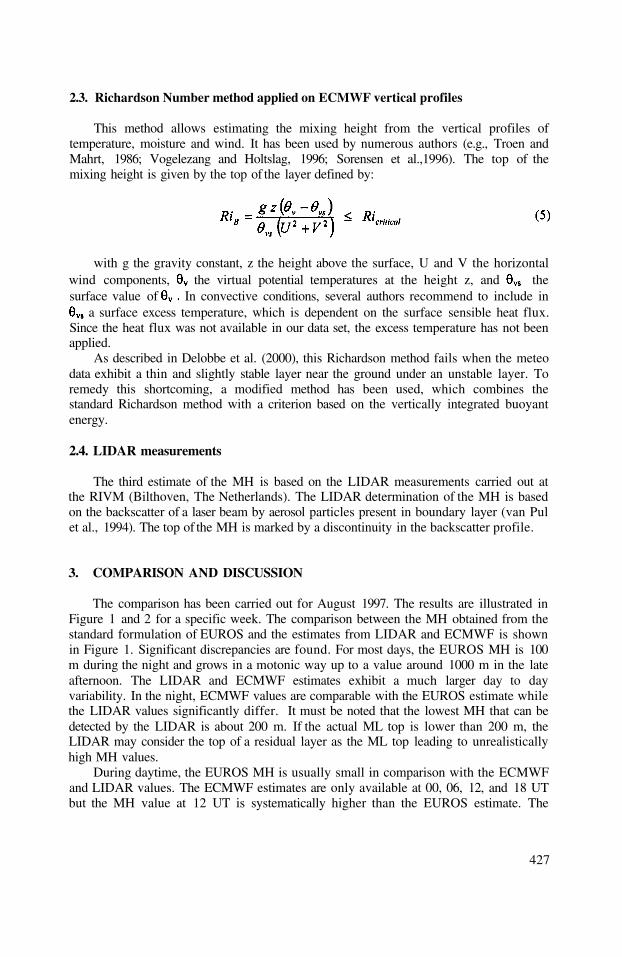
2.3. Richardson Number method applied on ECMWF vertical profiles
This method allows estimating the mixing height from the vertical profiles oftemperature, moisture and wind. It has been used by numerous authors (e.g., Troen andMahrt, 1986; Vogelezang and Holtslag, 1996; Sorensen et al.,1996). The top of themixing height is given by the top of the layer defined by:
with g the gravity constant, z the height above the surface, U and V the horizontalwind components, the virtual potential temperatures at the height z, and thesurface value of In convective conditions, several authors recommend to include in
a surface excess temperature, which is dependent on the surface sensible heat flux.Since the heat flux was not available in our data set, the excess temperature has not beenapplied.
As described in Delobbe et al. (2000), this Richardson method fails when the meteodata exhibit a thin and slightly stable layer near the ground under an unstable layer. Toremedy this shortcoming, a modified method has been used, which combines thestandard Richardson method with a criterion based on the vertically integrated buoyantenergy.
2.4. LIDAR measurements
The third estimate of the MH is based on the LIDAR measurements carried out atthe RIVM (Bilthoven, The Netherlands). The LIDAR determination of the MH is basedon the backscatter of a laser beam by aerosol particles present in boundary layer (van Pulet al., 1994). The top of the MH is marked by a discontinuity in the backscatter profile.
3. COMPARISON AND DISCUSSION
The comparison has been carried out for August 1997. The results are illustrated inFigure 1 and 2 for a specific week. The comparison between the MH obtained from thestandard formulation of EUROS and the estimates from LIDAR and ECMWF is shownin Figure 1. Significant discrepancies are found. For most days, the EUROS MH is 100m during the night and grows in a motonic way up to a value around 1000 m in the lateafternoon. The LIDAR and ECMWF estimates exhibit a much larger day to dayvariability. In the night, ECMWF values are comparable with the EUROS estimate whilethe LIDAR values significantly differ. It must be noted that the lowest MH that can bedetected by the LIDAR is about 200 m. If the actual ML top is lower than 200 m, theLIDAR may consider the top of a residual layer as the ML top leading to unrealisticallyhigh MH values.
During daytime, the EUROS MH is usually small in comparison with the ECMWFand LIDAR values. The ECMWF estimates are only available at 00, 06, 12, and 18 UTbut the MH value at 12 UT is systematically higher than the EUROS estimate. The
427

LIDAR provides hourly estimates of the MH. Large variations between two successivehours are regularly found.
Several causes of discrepancies between the three MH estimates can be mentioned.First of all, the method used in EUROS for the calculation of the MH has its ownlimitations. Errors may arise from the calculation of the surface meteorologicalparameters (Obukhov length, friction velocity and heat flux) but also from thedetermination of the MH from these parameters using expressions (1), (2) or (3). Themeteo input used for the calculation of the surface meteo variables, for example the 2m-temperature and the 10-m wind, also induce some errors. The meteo input used inEUROS results from a spatial interpolation from synoptic observations and a timeinterpolation from the 4 input times of these synoptical observations (00, 06, 12, 18 UT).This interpolation partly explains the fact that the MH diurnal cycles simulated byEUROS are much smoother than the observed diurnal cycles from the LIDAR. Anotherpossible cause of discrepancies arises from the fact that the LIDAR observations arelocal while, for ECMWF and EUROS, the estimate is an average over a grid cell, whosesize is about (for both models). The LIDAR measurements are much moresensitive to local conditions such as updraft or downdraft in convective conditions.
Concerning the estimates from ECMWF using a Richardson number method, a firstsource of error results from the relatively coarse vertical resolution of the ECMWF data:around 400m in the boundary layer. The Richardson method exhibits also someshortcomings (e.g., Seibert et al., 2000). In this study, the surface excess temperature hasnot been applied which may induce significant underestimation of the MH in convectivesituations. A previous study has shown the high sensitivity of the MH estimate to thesurface temperature used in Eq. (5) (Delobbe et al., 2000).
The determination of the MH from LIDAR measurements has also its limitations.We have already mentioned the minimal detectable value of 200 m, which may results inlarge errors for the night estimates. Another shortcoming is the large inaccuracies in caseof rain or if the amount of aerosol or trace gas in the boundary layer is too low.
Even if large discrepancies are found between LIDAR and ECMWF estimates, bothMH estimates are significantly higher than the results obtained with the standardformulation of EUROS. This formulation tends to underestimate the growth of themixing layer during the convective hours of the day. The new formulation (Eq. 4) takesinto account turbulence production due to surface friction and the entrainment heat fluxat the top of the convective layer as well. As shown in Fig. 2, this formulation results in adeeper growth of the mixing layer. Using the first set of parameters (a=0.2, b=2.5), theMH maximum at the end of the afternoon is about 200 m higher. As mentioned earlier,the values of the parameters a and b found in the literature vary within a large range. Inorder the get a first idea of the sensitivity to these parameters, two others parameter setshave been tested (a=0.4, b=5 and a=0.4, b=2.5). These values are recommended by someauthors as discussed in Seibert et al. (2000). The results are shown in Fig. 2. The MHmaximum at the end of the afternoon is now about 400 m higher than with the standardformulation. For the two parameter sets, the results are almost identical. It means that thevalue of the parameter a is more critical than the value of the parameter b. The parametera represents the ratio between the entrainment-layer and the surface-layer heat fluxes.
428
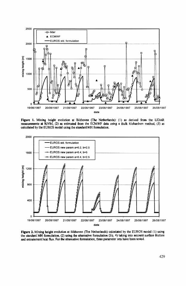
429

The entrainment effect appears to be predominant with respect to the surface frictioneffect. The highest MH values are obtained with a=0.4 and b=5. For this set ofparameters, Fig. 3 shows the comparison between the MH obtained at 17 UT with thenew formulation of EUROS and the LIDAR values averaged over two hours from 16 to18 UT. All the days of August 1997 for which LIDAR measurements are available areconsidered. The same Figure shows the results obtained with the standard formulation ofEUROS. The agreement between the EUROS results and the LIDAR measurements isbetter using the new formulation. However, the variation range of the EUROS MHvalues remains quite small compared with MH values derived from the LIDARmeasurements.
In this study, the sensitivity to the parameter has not been investigated. A fixedvalue has been used. This stability parameter plays however a key role in the descriptionof the mixing layer growth. It is related to the vertical gradient of potential temperaturejust above the mixing layer and could be in principle be determined from meteorologicalvertical profiles. However, this would require a significant extension of the amount ofmeteorological input data.
The intercomparison of MH estimates presented here concerns the month August1997. A deeper investigation would require to compare longer time series and ondifferent locations where observational data are available. Besides, the comparison waslimited here to the MH values. It would be useful to extend this comparison to somecrucial input variables used in the MH formulations, e.g. the surface sensible heat flux
430

and the friction velocity. This would allow to distinguish between the errors related thedeficiencies of the formulation itself and the errors due the inaccuracies in the inputmeteorological variables.
4. CONCLUSION
This study brings a contribution to the validation of MH parameterizations used inair quality models. The MH at Bilthoven (NL) simulated by EUROS has been comparedwith MH estimates from ECMWF meteorological vertical profiles and LIDARmeasurements for the month August 1997. It has been found that the EUROS standardformulation tends to underestimate the MH values and the day to day variability.Besides, the estimate based on a Richardson number method applied on ECMWF verticalprofiles is generally lower than the LIDAR estimate. A new MH formulation taking intoaccount the turbulence production due to surface friction and the entrainment heat flux atthe top of the convective layer has been implemented in EUROS. Our results show thatthis formulation allows a better representation of the mixing layer growth duringdaytime. However a deeper evaluation would require the intercomparison of various MHestimates on longer time periods and on different locations.
5. ACKNOWLEDGMENTS
This work is a contribution to EUROTRAC-2 subproject GLOREAM. It has beencarried out in the framework of the BelEUROS project (Implementation and extension ofthe EUROS model for policy support in Belgium) funded by the Belgian Federal Officefor Scientific Technical and Cultural Affairs.
6. REFERENCES
Batchvarova, E., and Gryning, S.E., 1991, Applied model for the growth of the daytime mixed layer,Boundary-Layer Meteorology, 56: 261-274.
Beljaars, A.C.M., and Holtslag, A.A.M., 1990, A software library for the calculation of surface fluxes over landsea, Environmental software, 5: 60-68.
Delobbe, L., O. Brasseur, and Mensink, C, 2000. Determination of the Mixing Height from ECMWF Data forUse in the Regional Photo-chemical Smog Model EUROS. To appear in Proceedings of EUROTRACSymposium, 2000.
Holtslag, A.A.M., and van Westrhenen, R.M., 1989. Diagnostic derivation of boundary layer parameters fromthe outputs of atmospheric models. Sci. Rep. KNMI WR 89-04.
Loon, M. van, 1996, Numerical methods in smog prediction, PhD thesis. University of Amsterdam, 148 pp.
Nieuwstadt, F.T.M., 1981, The steady-state height and resistance laws of the nocturnal boundary-layer: Theorycompared with Cabauw observations, Boundary-Layer Meteorology, 20: 3-17.
Seibert P., Beyrich, F., Gryning, S.-E., Joffre, S., Ramussen, A., and Tercier, P., 2000, Review andintercomparison of operational methods for the determination of the mixing height, Atmos. Environment,34: 1001-1027.
Sorensen, J.H., Rasmussen, A., and Svensmark, H., 1996, Forecast of atmospheric boundary layer heightutilised for ETEX real-time dispersion modelling, Physics and Chemistry of the Earth, 21: 435-439.
Tennekes, H., 1973, A Model for the Dynamics of the Inversion Above a Convective Boundary layer, J. Atmos.Science, 30: 558-567.
431

Troen, I. and Mahrt; L., 1986. A simple model of the planetary boundary layer. Sensitivity to surfaceevaporation. Boundary-Layer Meteorology, 37, 129-148.
van Pul, W.A.J., and Holtslag, A.A.M., and Swart, D.P.J.,1996, A comparison of ABL-heights inferredroutinely from lidar and radiosonde at noontime, Boundary-Layer Meteorology, 68, 173-191.
Vogelezang, D.H.P., and Holtslag, A.A.M., 1996, Evolution and model impacts of alternative boundary layerformulations. Boundary-Layer Meteorology, 81, 245-269.
432

DISCUSSION
A. BAKLANOV Your improvements and conclusions cover the Mixing height (MH)for unstable conditions only. For the nocturnal MH I do not see anyimprovement. Following your figures 1 and 2, it looks as if yourmodel puts a constant value of MH for night time (~ 100m),probably due to the fact that the usual parameterization does notwork satisfactory. Do you think it is a suitable method for calculationof the nocturnal MH ?
F. LEFEBRE The EUROS parameterisation for the MH takes a minimum MH of100 m. If during the night, the formulations give a MH below 100 m,it is corrected to 100m.In this presentation we have mainly been focusing on the mixingheight formulations during unstable and neutral conditions. We didnot analyze in detail the performance of the nocturnal MHparameterizations.
433

This page intentionally left blank
USING FUZZY NUMBERS TO TREAT PREDICTIONSFROM MORE THAN ONE MODEL
Bernard Fisher and Matt Ireland*
1. INTRODUCTION
The usual approach to the comparison of models is to compare the models’performance against some data sets and then to choose the model, which performs bestaccording to some criteria. In practice insufficient data usually exists to make a clearpreferred selection but for operational reasons one model is adopted. The selected modelis then used to make decisions about the appropriate regulation of new and existingsources. In this paper an alternative approach is proposed for situations when results fromseveral models are available assuming that each model has an acceptable level ofperformance. The basic assumption is that accepting the inevitable inaccuracies in eachmodel it is better to try to obtain a combined estimate based on all the informationavailable.
This may seem sensible qualitatively, but a decision maker has to make use of theextra information in a quantitative way. This can be illustrated by an example. Supposingthat one has the results of two models. If the results are presented as just two numbers,one does not have much extra information on which to base a decision. The twopredictions could be regarded as the either end of a range, so that the predictions providean indication, perhaps, of the likely range of predictions. The air quality objective mightlie above, below or within the range. Only in the case of the objective lying above therange would one be able to feel that there was no need for further investigation. A simplecase is one in which one has predictions from one or more dispersion models.
*Bernard Fisher, Environment Agency, National Centre for Risk Assessment and OptionsAppraisal, Steel House 11 Tothill Street London SW1H 9NF U.K. Matt Ireland, MottMacDonald, Victory House, Trafalgar Place, Brighton BN1 4FY U.K.
Air Pollution Modeling and Its Application XV, Edited byBorrego and Schayes, Kluwer Academic/Plenum Publishers, New York, 2002 435
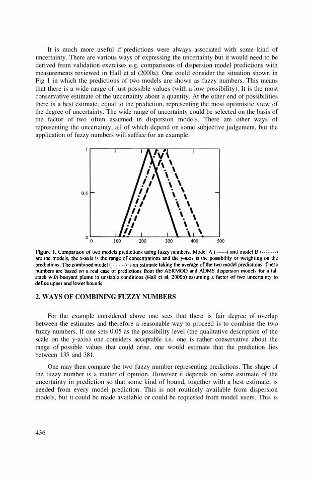
It is much more useful if predictions were always associated with some kind ofuncertainty. There are various ways of expressing the uncertainty but it would need to bederived from validation exercises e.g. comparisons of dispersion model predictions withmeasurements reviewed in Hall et al (2000a). One could consider the situation shown inFig 1 in which the predictions of two models are shown as fuzzy numbers. This meansthat there is a wide range of just possible values (with a low possibility). It is the mostconservative estimate of the uncertainty about a quantity. At the other end of possibilitiesthere is a best estimate, equal to the prediction, representing the most optimistic view ofthe degree of uncertainty. The wide range of uncertainty could be selected on the basis ofthe factor of two often assumed in dispersion models. There are other ways ofrepresenting the uncertainty, all of which depend on some subjective judgement, but theapplication of fuzzy numbers will suffice for an example.
2. WAYS OF COMBINING FUZZY NUMBERS
For the example considered above one sees that there is fair degree of overlapbetween the estimates and therefore a reasonable way to proceed is to combine the twofuzzy numbers. If one sets 0.05 as the possibility level (the qualitative description of thescale on the y-axis) one considers acceptable i.e. one is rather conservative about therange of possible values that could arise, one would estimate that the prediction liesbetween 135 and 381.
One may then compare the two fuzzy number representing predictions. The shape ofthe fuzzy number is a matter of opinion. However it depends on some estimate of theuncertainty in prediction so that some kind of bound, together with a best estimate, isneeded from every model prediction. This is not routinely available from dispersionmodels, but it could be made available or could be requested from model users. This is
436
the situation assuming that the model is being applied in the usual way, in order to obtainthe best estimate of the maximum ground-level concentration.
In contrast a screening model would be used in another way. A screening modelwould have a much wider range of possible predictions, without necessarily weightingthe maximum possibility (best estimate) towards the upper bound of the range. Thescreening model is used to incorporate all, or as many results, as possible. It is anticipatedthat normally the predictions of a screening model would have to be refined using a moreaccurate model, in order to reduce the range of possible predictions.
Fuzzy numbers can be manipulated in a consistent manner. They arise as arefinement of intervals which are rather crude encapsulations of uncertainty (Ferson,Root and Kuhn, 1999). For instance, intervals imply that although we cannot give aquantity’s value exactly, we can give exact bounds on the quantity. Fuzzy numbersgeneralise intervals. A fuzzy number can be thought of as a nested stack of intervalscontaining many levels of confidence about uncertainty. These levels of confidence rangebetween 0 (corresponding to the most conservative, widest interval) and 1 (the narrowestinterval, which assumes we are really good at making predictions). By definition, allfuzzy numbers must reach one and must be convex (single humped). The scale between0 and 1 is said to measure the possibility that a number is within the interval at aparticular level. This introduces the notion that possibilities can be graded. Fuzzynumbers and their arithmetic provide a simple and workable methodology that is valid forhandling non-statistical uncertainty in calculations.
In the application under consideration one might wish to take the average of the twoestimates and this leads to the combined estimate shown in the figure. As long as twofuzzy predictions contain a significant amount of overlap this seems a sensible way toproceed. However in situations where the fuzzy numbers are in ranges which do notoverlap one would conclude that the predictions are significantly different. Model A ispredicting values definitely lower than model B and taking some average would not beappropriate.
The reasons for a significant difference between model predictions are varied. Theycould arise because of an input error in one of the models. The models may be usingdifferent algorithms. For example the models may differ in the way they treat a plumenear the top of the boundary layer or what happens to a plume near the top of the hill.One model may predict zero concentration at the ground, while the other model maypredict substantial ground-level concentrations. The only way to deal with this situationis to consider the full specification of the model. This is the reason for the need fortransparency in the descriptions of models. Of particular interest are the algorithms forwhich a small variation in parameter values leads to a large change in concentration.
An alternative approach is combining two estimates is to consider that predictionsare uniformly distributed between the upper and lower bounds with equal probabilities.One can then obtain an average estimate by sampling each distribution at random. Thisassumes that one chooses values from the two distributions in an independent way to
437
obtain a combined distribution. If one chooses the 5 and 95 percentile points in thecombined distribution as bounds on the estimate, one obtains the range 167 to 344.
The conventional, simple approach is just to quote a range with the upper and lowerbounds chosen from the results from the best estimates of the two models e.g. between226 and 290. This is a start to defining uncertainty, but the measure of uncertainty isarbitrary depending on predictions of models in specific situations without regard tomodel performance. The range can appear unrealistically small. An alternative, simpleapproach is to take the range from the higher of the upper bound of the two predictionsand the lesser of the lower bounds of the two predictions, namely a range 113 to 425 inthis case. The fuzzy number approach gives a more bounded range, 135 to 381, while theassumption that there are random independent errors associated with each model givesthe smaller range, 167 to 344.
Thus taking ranges directly from models’ best predictions does not appear to give arealistic estimate of uncertainty. Taking the maximum range has the advantage ofsimplicity but may be regarded as encompassing too broad a range of possibilities. Theother two approaches are to some extent qualitative. Taking the mean of fuzzy numbers isrelated to taking the mean end points of intervals.
3. COMBINING TWO DIFFERENT MODELS
A similar idea can be adopted when one has separate models describing differentparts of an overall system. An example described previously is of the within anurban area, such as London. Fig 2 shows the from all road transport sources. Thisdoes not show the impact from the roads. One needs different models to treat pollutiondispersion on the local and regional scales. If one treats the urban area in an ideal way thelocal impact of emissions from major roads is not apparent. In an earlier paper methodsfor estimating roadside and background concentrations were described (Fisher and Sokhi,2000). These have been applied to an idealised, version of London in which three majorcircular roads are imagined to surround areas of the city: an inner ring road, an outer ringroad and an orbital road on the outskirts of the city. A cross-section of the annual average
concentration across the city is shown in Figure 3. The air quality standard of21ppb is exceeded within a central zone by the background concentration. However theexceedence around the outer ring road arises from the combined contributions of thebackground and the roadside concentrations. One precautionary way of estimating areasof exceedence taking account of uncertainty would be adopt an air quality standard of19ppb. This would have the effect of greatly enlarging the size of the central air qualitymanagement area. The gradient in the background concentration as a function of distanceis small so that small changes in the air quality standard produce large changes in the sizeof the air quality management area. In contrast the gradient in concentration close to theroad is large, so that small changes in the air quality standard applied have a smallereffect on the size of the air quality management area. Thus applying a discrete criterion todefine an air quality management area might be regarded as a far from ideal way oftaking account of uncertainty. The estimates of the air quality management area are notrobust and are very sensitive to qualitative estimates of the uncertainty.
438

An alternative approach is to assume that all estimates have some fuzziness oruncertainty associated with them, which will tend to smooth out the boundaries of anyarea to which a discrete, crisp criterion is applied. This approach can be applied to theexample of a road within a city using the measure of fuzziness applied in an earlier paper(Fisher and Newlands, 2000). In this paper a simple form for the multiplicative errorassociated with estimates of concentration C(x) at a point x of the formwas adopted where is the air quality standard. This had the advantage that functionscould be easily manipulated. The membership function of an air quality managementtakes the simple form where higher values of the membership functiondenote greater certainty that the point x lies within the air quality management area andvice versa. (This choice is preferable to a step function for which impliesexceedence and implies no exceedence.) It was possible to obtain an analyticalformula for the membership of an air quality management area based on the aggregate ofthe membership functions of background and roadside air quality management areasconsidered separately.
If this approach is applied to the air quality management area around the outer ringroad about 10km from the city centre, one obtains a membership function which lookslike that in Fig 4. The membership function or weighting is shown on the y-axis and thedistance from the city centre is shown on the x-axis in kilometres. Hence only distancesof a few hundred metres from the road are being considered. High values represent morecertainty that the point lies within an air quality management area and low values orweightings represent less certainty that the point lies within an air quality managementarea.
The result is dependent on choosing a form for the membership function and that theerrors in the roadside concentration are independent of the errors in the backgroundconcentration. The result also depends on the assumption that an aggregation function
439
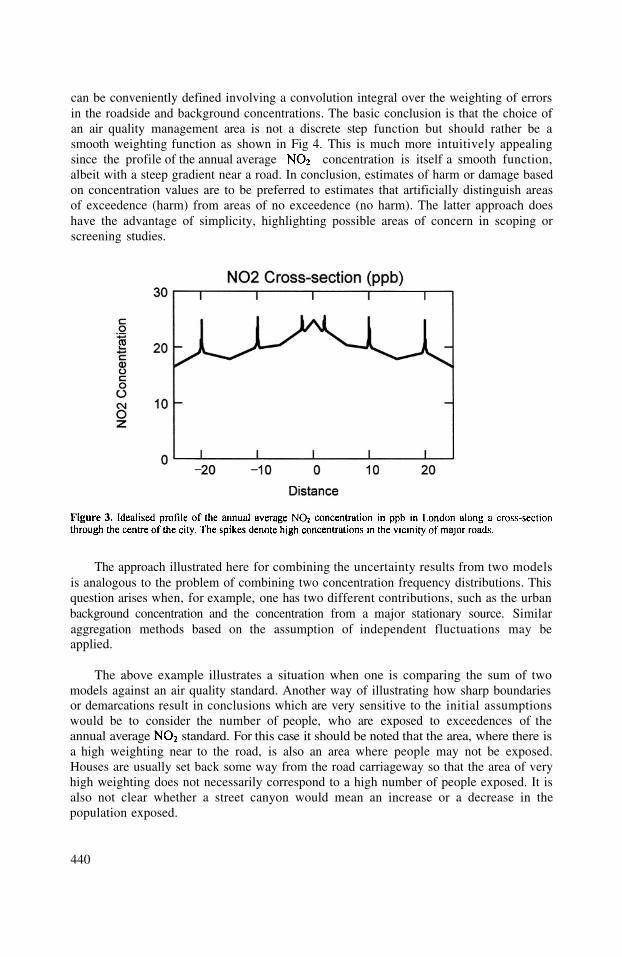
can be conveniently defined involving a convolution integral over the weighting of errorsin the roadside and background concentrations. The basic conclusion is that the choice ofan air quality management area is not a discrete step function but should rather be asmooth weighting function as shown in Fig 4. This is much more intuitively appealingsince the profile of the annual average concentration is itself a smooth function,albeit with a steep gradient near a road. In conclusion, estimates of harm or damage basedon concentration values are to be preferred to estimates that artificially distinguish areasof exceedence (harm) from areas of no exceedence (no harm). The latter approach doeshave the advantage of simplicity, highlighting possible areas of concern in scoping orscreening studies.
The approach illustrated here for combining the uncertainty results from two modelsis analogous to the problem of combining two concentration frequency distributions. Thisquestion arises when, for example, one has two different contributions, such as the urbanbackground concentration and the concentration from a major stationary source. Similaraggregation methods based on the assumption of independent fluctuations may beapplied.
The above example illustrates a situation when one is comparing the sum of twomodels against an air quality standard. Another way of illustrating how sharp boundariesor demarcations result in conclusions which are very sensitive to the initial assumptionswould be to consider the number of people, who are exposed to exceedences of theannual average standard. For this case it should be noted that the area, where there isa high weighting near to the road, is also an area where people may not be exposed.Houses are usually set back some way from the road carriageway so that the area of veryhigh weighting does not necessarily correspond to a high number of people exposed. It isalso not clear whether a street canyon would mean an increase or a decrease in thepopulation exposed.
440
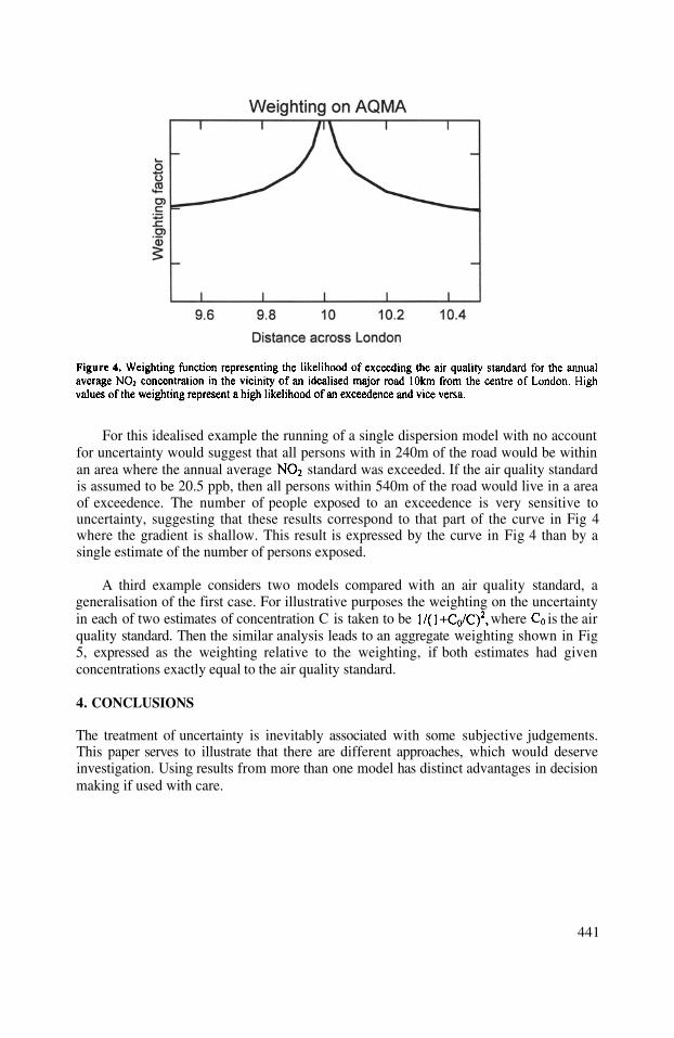
For this idealised example the running of a single dispersion model with no accountfor uncertainty would suggest that all persons with in 240m of the road would be withinan area where the annual average standard was exceeded. If the air quality standardis assumed to be 20.5 ppb, then all persons within 540m of the road would live in a areaof exceedence. The number of people exposed to an exceedence is very sensitive touncertainty, suggesting that these results correspond to that part of the curve in Fig 4where the gradient is shallow. This result is expressed by the curve in Fig 4 than by asingle estimate of the number of persons exposed.
A third example considers two models compared with an air quality standard, ageneralisation of the first case. For illustrative purposes the weighting on the uncertaintyin each of two estimates of concentration C is taken to be where is the airquality standard. Then the similar analysis leads to an aggregate weighting shown in Fig5, expressed as the weighting relative to the weighting, if both estimates had givenconcentrations exactly equal to the air quality standard.
4. CONCLUSIONS
The treatment of uncertainty is inevitably associated with some subjective judgements.This paper serves to illustrate that there are different approaches, which would deserveinvestigation. Using results from more than one model has distinct advantages in decisionmaking if used with care.
441
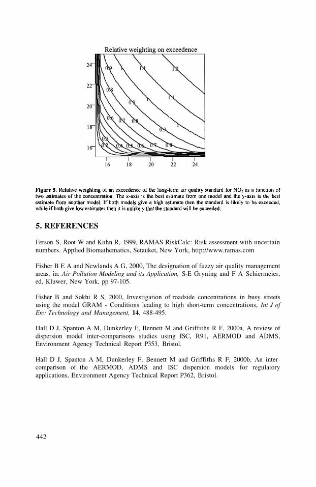
5. REFERENCES
Ferson S, Root W and Kuhn R, 1999, RAMAS RiskCalc: Risk assessment with uncertainnumbers. Applied Biomathematics, Setauket, New York, http://www.ramas.com
Fisher B E A and Newlands A G, 2000, The designation of fuzzy air quality managementareas, in: Air Pollution Modeling and its Application, S-E Gryning and F A Schiermeier,ed, Kluwer, New York, pp 97-105.
Fisher B and Sokhi R S, 2000, Investigation of roadside concentrations in busy streetsusing the model GRAM - Conditions leading to high short-term concentrations, Int J ofEnv Technology and Management, 14, 488-495.
Hall D J, Spanton A M, Dunkerley F, Bennett M and Griffiths R F, 2000a, A review ofdispersion model inter-comparisons studies using ISC, R91, AERMOD and ADMS,Environment Agency Technical Report P353, Bristol.
Hall D J, Spanton A M, Dunkerley F, Bennett M and Griffiths R F, 2000b, An inter-comparison of the AERMOD, ADMS and ISC dispersion models for regulatoryapplications, Environment Agency Technical Report P362, Bristol.
442

DISCUSSION
S. RAFAILIDIS
B. FISHER
In the presentation you tackle with the uncertainty in theconcentrations. If on top of this you add the uncertainty in the healtheffects of the concentrations, does your final result become more“focused” or widens out ?
Taking into account the uncertainty in the health effect would notwiden the overall uncertainty, as the health effect is usuallyinterpreted as a threshold air quality standard. In reality theepidemiological data which is used to derive the air quality standardis uncertain. Hence if our assessment includes there, then the overalluncertainty is increased.
443

This page intentionally left blank

NARSTO MODEL COMPARISON AND EVALUATIONSTUDY (NMCES)
A major study comparing regional air quality modeling systems used for regulatorypurposes in the USA and Canada is being conducted under the auspices of NARSTO.Groups from the Meteorological Service of Canada, US Environmental Protection Agency,New York State Department of Environmental Conservation, North CarolinaSupercomputing Center, Environ International, and ICF Consulting are participating. Thesegroups, their sponsors, the models they used and the gridding schemes employed are shownin Table 1.
*D. Alan Hansen, EPRI, P.O. Box 10412, Palo Alto, CA 94303, USA
Air Pollution Modeling and Its Application XV, Edited byBorrego and Schayes, Kluwer Academic/Plenum Publishers, New York, 2002 445
D. Alan Hansen*
1. INTRODUCTION
The opportunity for such a study presented itself when, stimulated by the need to meetregulatory milestones for attainment of national standards and objectives for ozone in thetwo countries, many public and private groups modeled time periods in July 1995 inoverlapping domains covering most of eastern North America. By taking advantage of thisrare opportunity, the comparability of modeling results between Canadian and Americanenvironmental agencies and among public and private groups could be established withoutundertaking an effort of much larger proportions.
To guide the study, a Working Group was organized and comparison protocols weredeveloped by sub-working groups for emissions, meteorological and air quality modeling.EPRI was selected to coordinate the study and produce the comparison tables and graphics.Each of the protocols has been implemented to a greater or lesser degree, depending onresources and priorities, with the higher priority given to the air quality model comparison.
The study was conceived to take place in two phases. In the first phase the models wereto be compared in their “native” mode, i.e., using the same input files and modelconfigurations that each group used in their individual assessments, based on modeling a 9to 14-day period in July 1995. The planners believed that, with a minimal amount of extraeffort, existing model output files could readily be used for the comparison and valuableinformation would be gained on the relative performance of these disparate models, each ofwhich has been used in exercises having significant policy implications. As the study hasunfolded, the first phase has not been as straightforward as initially anticipated. Firstly,modeling errors were discovered that motivated some participants to withdraw theirmodeling files for replacement with new corrected files. Secondly, the Working Groupasked two participants that had used two-way nested grids to run additional simulations withthe entire domain coarsely gridded so that coarse and fine results over the same geographicalareas could be compared. Thirdly, one participant decided to rerun its models at a finer gridover the entire domain. And finally all participants were asked to rerun their models withseparate across-the-board 50% reductions in anthropogenic NOx and volatile organiccompound emissions. As a result, completion of Phase 1 has been delayed by at least twoyears from the originally planned date, with an expected completion in late 2001.
The idea of a second phase was based on the realization that comparing models run intheir native mode would provide insufficient information to diagnose why models mightyield different results. A more comprehensive approach would need to be taken. Further, itwould recognize the anticipated widespread desire to compare models with an aerosolsimulation capability. Thus, in Phase 2 regional tropospheric aerosol models would becompared using harmonized model inputs. “Harmonization” means that models would beexercised, for example, on identical domains, employing the same horizontal gridding,topography, land use, vegetation distributions and emissions inputs. Meteorological inputswould be as similar as possible, consistent with maintaining mass conservation.Additionally, participating models would be expected to have a process analysis capabilityto facilitate diagnostic analyses. Whether or not there will be a send phase remains to bedetermined.
This paper describes Phase 1. The next section enumerates the modeling domains andsub-domains selected for comparison to determine if model performance variedgeographically. That is followed by descriptions first of how the emissions files used asinputs to the air quality models and then how the meteorological files used to drive the airquality models were compared. Then the approach to comparing the air quality models is
446
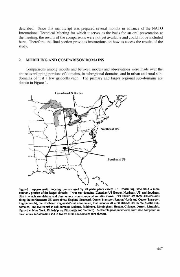
described. Since this manuscript was prepared several months in advance of the NATOInternational Technical Meeting for which it serves as the basis for an oral presentation atthe meeting, the results of the comparisons were not yet available and could not be includedhere. Therefore, the final section provides instructions on how to access the results of thestudy.
Comparisons among models and between models and observations were made over theentire overlapping portions of domains, in subregional domains, and in urban and rural sub-domains of just a few gridcells each. The primary and larger regional sub-domains areshown in Figure 1.
447
2. MODELING AND COMPARISON DOMAINS

Resource constraints forced an abbreviated version of the emissions comparisonprotocol to be conducted. It was comprised of each participant responding to thequestionnaire shown in Table 2 and providing aggregated emissions totals for NOx andselected VOCs for the period 7-15 July 1995 for the states of MI, TN, MA, MD and NJ.This information would at least document details of how the emissions files were generatedand allow a spot check for comparability among emissions files to be performed.
448
3. EMISSIONS COMPARISON
Initial comparisons found large apparent differences between NOx and some VOCemissions totals reported by three participants. After diagnosing the factors contributing tothese differences, corrections were made and the models rerun. It is the corrected files thatare included in the study archives.
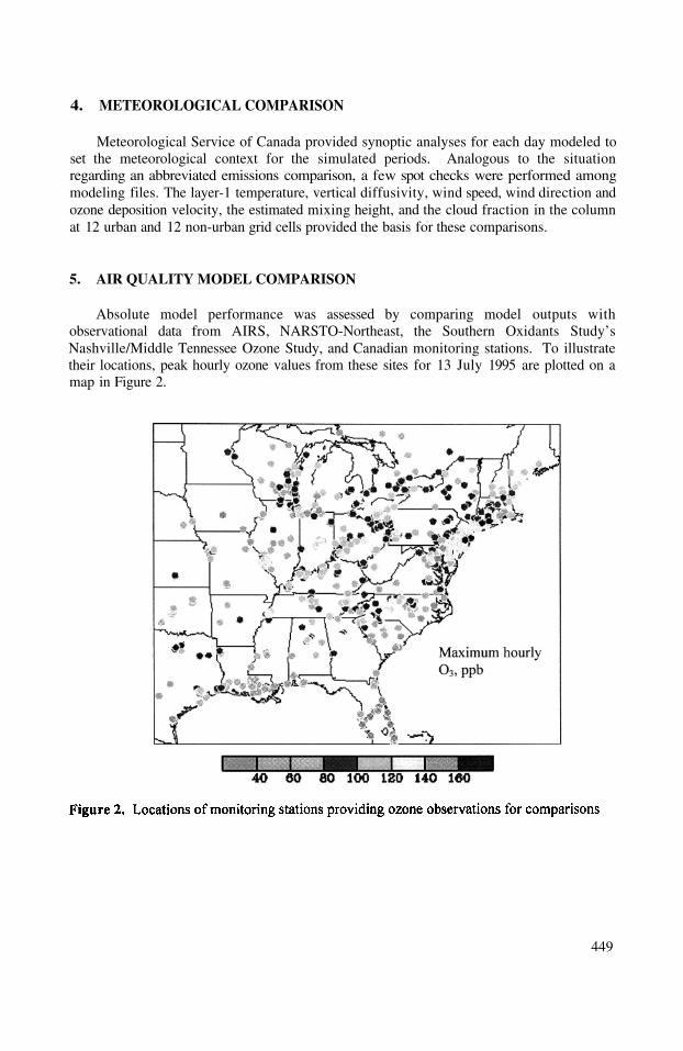
Meteorological Service of Canada provided synoptic analyses for each day modeled toset the meteorological context for the simulated periods. Analogous to the situationregarding an abbreviated emissions comparison, a few spot checks were performed amongmodeling files. The layer-1 temperature, vertical diffusivity, wind speed, wind direction andozone deposition velocity, the estimated mixing height, and the cloud fraction in the columnat 12 urban and 12 non-urban grid cells provided the basis for these comparisons.
Absolute model performance was assessed by comparing model outputs withobservational data from AIRS, NARSTO-Northeast, the Southern Oxidants Study’sNashville/Middle Tennessee Ozone Study, and Canadian monitoring stations. To illustratetheir locations, peak hourly ozone values from these sites for 13 July 1995 are plotted on amap in Figure 2.
449
4. METEOROLOGICAL COMPARISON
5. AIR QUALITY MODEL COMPARISON

In Section 2, the modeling sub-domains selected for comparing the models’performance were described. The basis for these selections was the desire to explore thepossibility that, as configured, model performance might differ as a function of averagingtime or time of day, between urban and rural areas, between coastal and inland areas and inwidely separated geographic areas having distinct emissions distributions, topography ormeteorological regimes. A number of metrics were selected as indicators of modelperformance. These are listed for ozone comparisons in Table 3.
Two types of statistical tables are planned. The regulatory statistics are thoserecommended as performance measures for hourly peak predictions by the US EPA(1991), with the addition of 8-hour averages and of concentrations thresholds of 20, 40, and60 ppb The statistics for scientific analyses, will be calculated without applyingthresholds, over different time windows to investigate the models’ ability to simulate notonly peak concentrations but also those at night and in the early morning before theboundary layer is well mixed. Graphics will include contour map plots of observed andsimulated concentrations, color-coded map plots of biases, time series plots of simulated andobserved values averaged over the various sub-domains for ozone and representing the grid
450

cells having observations for NOx and selected VOCs., and scatter plots of simulated versusobserved air quality variables and of one model’s simulated values versus those of othermodels.
By the time this paper is presented at the NATO International Technical Meeting,comparison results should be available and included in the presentation. Ultimately thecomparison data and other documentation of methods and models will be archived in theNARSTO data archive (http://eosweb.larc.nasa.gov/project/narsto/table_narsto.html). Dataused for air quality comparisons and the comparison products expected to be available arelisted in Tables 4 and 5. In the interim, information can be obtained from the author (Seesection 9.)
451
6. DATA AVAILABLE

US EPA, 1991. Guidance for Regulatory Application of the Urban Airshed Model. Office of Air Quality Planningand Standards, Research Triangle Park, NC 27711. July 1991.
The author expresses his appreciation to EPRI, Meteorological Service of Canada,Tennessee Valley Authority, Texas Natural Resources Conservation Commission, andOntario Ministry of the Environment for direct financial support of the project and to theCoordinating Research Council, the Southeast States Air Resource Managers,Meteorological Service of Canada, the US Environmental Protection Agency, the New YorkState Department of Environmental Conservation, and Southern Company for sponsoringinitial modeling from which model comparison files were derived. In addition, theparticipating organizations provided substantial in-kind support in staff and resources. Theassistance of Naresh Kumar of EPRI in co-managing the project is gratefully acknowledged,as is the processing of modeling data files into statistical tables and graphics provided bySonoma Technology, Inc., led by Neil Wheeler. Other EPRI staff who contributedsubstantially to the effort include Mohan Gupta, George Bonne, and Randall Takemoto-Hambleton. Special recognition is given to Maris Lusis and S. Venkatesh of MSC forsuggesting the study and to their colleagues, Mike Moran and Janusz Pudykiewicz formanaging the emissions comparisons and CHRONOS modeling, respectively; and to JeffArnold and Robin Dennis of NOAA/USEPA, Rohit Mathur of NCSC, Gopal Sistla ofNYDEC, Ralph Morris of Environ and Sharon Douglas of ICF Consulting for managingtheir organization’s participation in the study.
Contact Alan Hansen, EPRI, P.O. Box 10412, Palo Alto CA, 94303, USA. Telephone:650.855.2738, fax: 650.855.2950, email: [email protected].
452
7. REFERENCES
8. ACKNOWLEDGEMENTS
9. FURTHER DETAILS

Was an attempt made to make an evaluation of the observationsbefore they were used in the model evaluation ?
Not explicitly. However, we understand that the observationsthemselves have uncertainties associated with measurement error andvariability within grid cells. Therefore we are generally usingstatistics based on averaging over many grid cell-site combinationsand interpreting the results in a relative rather than absolute sense.
453
DISCUSSION
P. BUILTJES
A. HANSEN

This page intentionally left blank
The surface roughness length is one of a few most important parameters determiningthe deposition velocity of airborne particles. In this context the mid-latitude flat ruralareas could be divided into two substantially different categories: (1) forest and (2) openareas. The roughness difference is most dramatic, if the snow cover is thick enough tocover the grass and other small roughness elements at open sites. The typical roughnesslength of boreal and sub-boreal forest is 0.5 – 1 m, whereas the roughness length of snowsurface does not usually exceed 0.001 m (except due to snow blown up by the strongwind). Consequently, the atmospheric resistance to the deposition is much larger over theopen areas and therefore lower dry deposition velocities are expected.
The early experimental studies (see McMahon and Denison, 1979) support the aboveconsiderations despite the large scatter of results. Several model runs (Ruijgrok et al.,1995) show, that the deposition velocity of particles over the forested land can be tens oftimes higher than over the open one. The difference depends on particle size, beingclearly larger for particles sized several micrometers than for the sub-micron ones. Donatand Ruck (1999) provided the wind tunnel simulations of deposition of sub-micronparticles onto the ground below the trees and found the deposition fluxes 20 – 60 %(depending on tree crown shape) larger than onto the open surface in similar conditions.Although several field and wind tunnel experiments have been carried out recently, themain attention is paid to the deposition of small particles in the nearly neutralstratification.
The present study is focused to the deposition of mineral particles sized aboutas average. Such particles occur typically in the fly ashes of thermal power plants and cancontain remarkable amounts of sulphates, alkaline oxides and radionucleides. A natural
* Marko Kaasik, Tartu Observatory, Tõravere, Tartumaa, 61602 Estonia.
Air Pollution Modeling and Its Application XV, Edited byBorrego and Schayes, Kluwer Academic/Plenum Publishers, New York, 2002
INFLUENCE OF UNDERLYING SURFACEROUGHNESS TO THE DEPOSITION OF AIRBORNEPARTICLES IN NORTHERN WINTER CONDITIONS
Marko Kaasik*
1. INTRODUCTION
455

medium-term collector – snow cover – is used to trace the deposition fluxes. The role ofdry and wet deposition is discussed.
A case study was carried out in 1996 to clarify the effect of forest-induced roughnessto the deposition flux of airborne fly ash particles (Kaasik et al, 2000). The research siteswere chosen in the north-eastern part of Estonia, at distances of 1 – 130 km from twolarge thermal power plants (total maximum capacity 3 GW), consuming Kukersite oilshale. The Kukersite oil shale fly ash has rather specific elemental composition (Häsänenet al. 1995): 15 – 22% Ca, 6 – 10 % K, several trace metals, 5 – 6% S. As most of metalsin the fly ash are in carbonaceous form, the reaction of fly ash solution is stronglyalkaline.
The measurement was based on snow samples taken from 15 sites (6 from forested, 7from open and 2 from mixed landscape) and representing 3 snow accumulation episodes(72 days in total) during one winter and analysed for main anions, cations and tracemetals. The most remote sites (one forested and one open) were considered asbackground ones. Knowing the chemical composition of oil-shale fly ash, the depositionfluxes of fly ash particles were reconstructed.
The wind during the snow accumulation was blowing predominantly from southerndirections, which is typical for the research area and season. The average waterequivalents of all three snow layers matched well with meteorological observations ofprecipitation amounts (Figure 1), which indicates, that no snow was lost due to melting.The average temperatures of the snow accumulation episodes were –8.9, –8.0 and
456
2. METHODS

–11.8 °C, no substantial thawing was registered. No systematic or considerablediscrepancies between snow accumulation at forested and open sites was found.
The deposition measurements were accompanied by the runs of air pollutiondispersion and deposition model AEROPOL for the same episodes. The AEROPOLmodel (Kaasik, 1996) is a Gaussian plume model developed at Tartu Observatory,Estonia. The simple bulk deposition scheme includes only gravitational settling andprecipitation scavenging for large particles, no landscape-dependent effects are included.The boundary-layer parameterisation is based on the Pasquill stability classes, which,although coarse, enables us to manage with routine (ground-based) meteorologicalobservations only. A highly uncertain initial parameter for model calculation was theaerodynamic diameter of a ash particle. Earlier measurements (Aunela et al., 1995)suggest the particle sizes in the order of but due to high humidity of the flue gasesconsiderably larger particles are expected after condensation and subsequent freezing ofwater. The effective particle size is applied in this study, the sensitivity analysis isperformed.
The results of the case study show that the deposition fluxes of fly ash particles overthe forested areas are systematically higher than over nearby open (bog) areas (Figure 2),although the precipitation amounts were found nearly equal for both landscape types (seeSection 2).
Considerable differences appear during each of three time episodes. Most likely thedifferences appear due to different dry deposition velocities. In the beginning of winter,when the nearly neutral thermal stratification prevailed due to mainly cyclonal weather,the deposition difference between the open and forest sites is small. During the midwinterthe cyclonal weather gradually changed to more anticyclonal, with multiple rapid changesof air temperature and stratification. The corresponding deposition curve for forest is wellabove the one for open landscape. The total deposition is larger than for first episode dueto larger share of northern and northeastern winds. During the late winter the weather wasthe most anticyclonal of these three episodes. Moderate snowfalls occurred between coldand calm days. The wind was blowing quite frequently from the direction of power plant,but less than 4 mm of precipitations occurred during such events. The deposition at forestsites is 1.5 – 2 times larger than in the open ones.
457
3. RESULTS
3.1. Deposition measurements
3.2. Model estimations
The modelled and measured deposition fluxes at the measurement sites are comparedin Figure 3. For comparison the mixed sites (complicated pattern of woodland and openland) near power plants are added. The north-eastern direction should be understoodunder the negative distance. Another (called Baltic) power plant is located nearly at 17km northeast (i.e. near the leftmost snow site) from the Estonian one.

The model predicts dominating wet deposition during the early winter, both dry andwet deposition in midwinter and highly dominating dry deposition during late winter.These results match well with the interpretation given in previous subsection. The totaldeposition near the sources is more or less matched despite large scatter of bothmodelling and measurement results. Away from the sources, the model tends tounderestimate the deposition. A part of this underestimation could be explainedwith the nearly similar emissions from local sources. The measured deposition fluxesin background sites (far right in Figure 3), however, are less than the typical differencebetween measured and modelled deposition at moderate distances.
The mismatch of modelled and measured fluxes was exceptionally high during thesecond episode, for which the model failed to reproduce the main direction of fly ashtransport. The probable reason is the overestimation of boundary-layer wind shear by 10– 20 degrees for certain dispersion events.
458

459
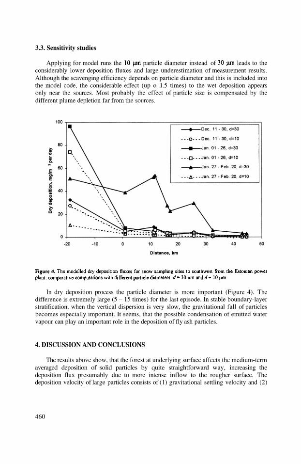
Applying for model runs the particle diameter instead of leads to theconsiderably lower deposition fluxes and large underestimation of measurement results.Although the scavenging efficiency depends on particle diameter and this is included intothe model code, the considerable effect (up o 1.5 times) to the wet deposition appearsonly near the sources. Most probably the effect of particle size is compensated by thedifferent plume depletion far from the sources.
In dry deposition process the particle diameter is more important (Figure 4). Thedifference is extremely large (5 – 15 times) for the last episode. In stable boundary-layerstratification, when the vertical dispersion is very slow, the gravitational fall of particlesbecomes especially important. It seems, that the possible condensation of emitted watervapour can play an important role in the deposition of fly ash particles.
The results above show, that the forest at underlying surface affects the medium-termaveraged deposition of solid particles by quite straightforward way, increasing thedeposition flux presumably due to more intense inflow to the rougher surface. Thedeposition velocity of large particles consists of (1) gravitational settling velocity and (2)
460
3.3. Sensitivity studies
4. DISCUSSION AND CONCLUSIONS

turbulent part. For smooth surfaces (like open snow surface) the deposition velocitiesclose to the settling velocity are suggested for particles considerably larger than(see e.g. McMahon and Denison, 1979), i.e. the turbulent part is small compared to thegravitational one. The detail deposition models give controversy results for deposition oflarge particles to the forest: from nearly settling velocity to 10 – 20 times larger values by
km from the Estonian power plant was about per day or about a half of totaldeposition flux (assuming it negligible for the open snow surface, but not for forest).Consequently, the deposition velocity is at least twice larger than the settling velocity, butcan be much larger, if the share of wet deposition is considerable. The model runsuggests, that wet deposition consists 20 – 35 % of total one. Therefore the ratio ofdeposition velocity to the settling velocity can be in the range of 2.5 – 4. For other twoepisodes the turbulence-dependent part of dry flux is less, but the model-suggested shareof dry deposition is considerably less as well. Therefore, the above ratio can be in thesame range. This result is in agreement with Bache’s one (Bache, 1979, referred byRuijgrok et al., 1995).
The forest and open land pattern can affect the meso-scale and large-scale admixturetransport processes through the friction at the underlying surface. It was shown (Kaasik,2001), that large uncertainties of the underlying surface forest fraction affect seriously theturbulent dispersion calculation results through entire boundary layer and even in thelower troposphere above it. The effects of (1) deposition efficiency and (2) wind drag athigher altitudes are summarised in large scale. Therefore the land use data sets forregularly used atmospheric models, however, have to be critically reviewed andimproved (Kaasik and Roosaare, 2000).
461
ACKNOWLEDGEMENTS
The results are based to the field work and theoretical studies granted by the EstonianScience Foundation (research grant No. 186). Author is grateful to the NorwegianInstitute for Air Research for chemical analyses.
REFERENCES
L. Aunela, E. Häsänen, V. Kinnunen, K. Larjava, A. Mehtonen, T. Salmikangas. Emissions from Estonian oilshale power plant. Oil Shale, 12, 2, pp. 165 – 177 (1995).
D. H. Bache, Particulate transport within plant canopies (II). Prediction of deposition velocities. Atm. Environ.,13, pp. 1681 – 1687(1979).
J. Donat, B. Ruck. Simulated ground deposition of fine airborne particles in an array of idealized tree crowns.Water, Air and Soil Pollution 93, pp. 469 – 492 (1999).
E. Häsänen, L. Aunela., V. Kinnunen, K. Larjava, A. Mehtonen, T. Salmikangas, J. Leskelä and J. Loosaar. In:World Clean Air Congress. Vol. 1, edited by M. Tolvanen, P. Anttila and J. Kämäri (The Finnish Air
Pollution Prevention Society, Espoo, 1995), pp. 057– 060.
different models for particles (overview by Ruijgrok et al., 1995). The depositionvelocity is positively related to the friction velocity.
The results above (Figure 2) enable us to estimate approximately the turbulent part ofdeposition flux, leaving the share of gravitational settling and wet deposition quiteuncertain. For the late winter episode the turbulence-dependent deposition flux at 10 – 12

M. Kaasik. Influence of underlying surface forest fraction to the meso-scale wind fields and dispersionconditions. In: Air Pollution Modelling and Simulation, edited by B. Sportisse, Springer (2001, in print).
M. Kaasik. Atmospheric dispersion and deposition of technogenic calcium: model estimation and fieldmeasurement, Proc. Estonian Acad. Sci. Ecol., 1/2, 41 – 51 (1996).
M. Kaasik, J. Roosaare. New Estonian and Eastern Baltic region land use database for HIRLAM. HIRLAMNewsletter 35, pp. 157-162 (2000).
M. Kaasik, R. Rõõm, O. Røyset, M. Vadset, Ü. Sõukand, K. Tõugu and H. Kaasik. Elemental and base anionsdeposition in the snow cover of north-eastern Estonia. The impact of industrial emissions, Water, Air, andSoil Pollution 121, 324-366 (2000).
T. A. McMahon, P. J. Denison. Empirical atmospheric deposition parameters – a survey. Atm. Environ., 13, pp.571–585 (1979).
W. Ruijgrok, C. I. Davidson, K. W. Nicholson. Dry deposition of particles. Implications and recommendationsfor mapping of deposition over Europe. Tellus 47B, pp. 587 – 601 (1995).
462

Can you explain the increased modeled oscillations and stnadarddeviation with distance of the deposition when you increased theparticle size from to
Modelling results are oscillating due to interference of another powerplant: a transect from one power plant crosses the plumes of theother (there were not many plumes modelled).The deposition fluxes were unrealistically low, but therelative oscillations were in the same range than for case.
463
DISCUSSION
D. HANSEN
M. KAASIK

This page intentionally left blank

A STUDY OF SO2 DISPERSION AROUND ATHERMOELECTRIC POWER PLANT
IN THE SOUTH OF BRAZIL
Osvaldo L. L. Moraes, Rita C. M. Alves, Rodrigo Silva, Adriano C.Siqueira, Patrícia D. Borges, Tiziano Tirabassi, Umberto Rizza1
1.
As part of the Presidente Medici Thermoelectric Power Plant plume modelvalidation study, a major field measurements program was carried out at Candiota town,south of Brazil. Project Candiota was a cooperative field study leaded by theMicrometeorological Laboratory from the Physics Department of the Federal Universityof Santa Maria (UFSM - Brazil) with groups of scientists from Universidade de SãoPaulo (Brazil), Instituto di Scienze dell´Atmosfera e dell´Oceano and Instituto per loStudio dell' Inquinamento Atmosferico e l'Agrometeorologia both from Italy. The projecthad support of the Companhia Estadual de Energia Elétrica (CEEE) and Companhia deGeração Térmica de Energia Elétrica (CGTEE), owners of the thermoelectric, and fromthree differentes research foundations of Brazil (FAPERGS, FAPESP and CNPq) andfrom the Consiglio Nazionale delle Ricerche (Itália). The objective was to collect acomprehensive, meteorological diffusion and dispersion database to be used to evaluateand improve selected diffusion, and dispersion models. Candiota consists of an ideallaboratory to test and to validate dispersion models for a series of reasons, among whichwe can point: the thermoelectric is the only source of some pollutants in the whole area,e.g. SO2; the source is punctual and emits continually with a very known rate; thetopography of the area is essentially homogeneous. The pollutant is emitted withbuoyancy from a tower at a height of 150 m.
Over 1,000 hr of intensive observations were made during five field campaigns(winter 1994, summer 1995, autumn 1995, spring 1995 and winter 1999). Each fieldexperiment was made during two weeks. Meteorological data was collected over a 2-
1 Osvaldo L. L. Moraes, Rodrigo Silva, Adriano C. Siqueira, Patrícia D. Borges,Universidade Federal de Santa Maria. Departamento de Física, 97119.900 Santa Maria,Brazil, Rita C. M. Alves, Universidade Federal do Rio Grande do Sul, CEPSRM, PortoAlegre, BrazilTiziano Tirabassi, ISAO, Bologna, Italy, Umberto Rizza, ISIATA, Lecce,Italy.
Air Pollution Modeling and Its Application XV, Edited byBorrego and Schayes, Kluwer Academic/Plenum Publishers, New York, 2002 465
INTRODUCTION

week time resulting in a full set of daytime period and the database comprisesmeasurements of wind speed, wind direction, turbulence, temperature, humidity,pressure, solar radiation, the boundary layer structure and upper-air-soundings. Thecampaign site (31.40S, 53.70W, 250 m above sea level) has previously been used for anumber of experiments related to research on atmospheric boundary layer (Moraes et al1998, Moraes 2000a). The base is located in a region known as the South AmericaPampa. The Pampa is the part of SA that covers all Uruguay territory, the south of Braziland northwest of Argentina. The area around the experimental site is flat for over 10 Kmin every direction.
In this paper we study the environmental impact in the region due to thethermoelectric emissions with a numerical 3D model and with a non-gaussian puffmodel. The performances of the models are evaluated with boundary layerparameterization derived from the fields campaigns.
2. THE MODELS
2.1 The Puff Model
The puff model is described in a series of papers (Tirabassi and Rizza, 1997a,Tirabassi and Rizza 1997b) and here we only outline its principal characteristics.
The advection diffusion equation describing the time evolution of the crosswind-integrated concentration due to an instantaneous release at time t = 0 by an elevated
source placed at (0,0,1), in a horizontally homogeneous atmospheric boundary layer is
Considering that is exponentially small at asymptotic distances from thesource the moments of its distribution on any horizontal plane may be defined as
we obtain the following set of equations for the time evolution of the moments
with the following initial and boundary conditions
466
where is a non-negative integer. Multiplying equation (1) by and integrating it in

Tirabassi and Rizza (1997) solved this set of equations using the Gram-Charlierexpansion of type A truncated to the fourth order and recovered the concentration field.They obtained
In this paper the lateral diffusion was parameterized by means of a Gaussian-type factor and the concentration at any point was calculated as
where represents the mean square particle displacement along the y – axis with the
condition
2.2 The Numerical Model
The numerical model use a solution of the advection diffusion equation of airpollution in the atmosphere, that is essentially a statement of conservation of thesuspended material and can be written:
The equation is solved using a finite-difference scheme. A forward-in-time,upstream-in-space scheme is used for the advection terms. For diffusion terms, a semi-implicit centered scheme with weight 0.75 on a future time step is used. The lower and
467
where and and are theskewness and kurtosis defined as

top boundary conditions was the same as used in the first model. For the results presentedin this paper the vertical resolution of the grid was defined as where H is theboundary layer height and N = 30 for all simulations. The horizontal grid has 100 x 100points linearly spaced with 100 m of distance between them. The time step is 3 s.
3. THE BOUNDARY LAYER PARAMETERIZATIONS
In order to evaluate the diffusion coefficients that are in eqs (4) and (6), we haveused the boundary layer parameterization proposed by Moraes (2000b). Thisparameterization is based on Hanna (1968) assumption that the mixing efficiency of theair is completely determined by the properties of the vertical velocity spectrum, and that
the parameters and are sufficient to describe the vertical velocity spectrum.
Then it follows from dimensional reasoning that the vertical eddy diffusivity coefficientmay be written as
where is a constant equal to 0.09.From the measurements done in the surface layer and using local scalings
assumptions we obtained for the vertical turbulent diffusion coefficient in the wholeboundary layer the following expressions for stable and convective regimes
The lateral diffusion, for the puff model, is obtained through values
proposed by Briggs (1973) for open country and given by
where is a constante equal to (0.22, 0.16, 0.11, 0.08, 0.06, 0.04) if the Pasquillstability is (A, B, C, D, E, F) respectively. For the numerical simulations the lateral eddydiffusion coefficient is estimated as in unstable conditions and as in
neutral-stable conditions, where is the maximum of
468
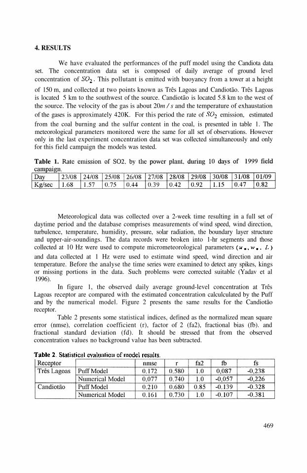
4. RESULTS
We have evaluated the performances of the puff model using the Candiota dataset. The concentration data set is composed of daily average of ground levelconcentration of This pollutant is emitted with buoyancy from a tower at a height
of 150 m, and collected at two points known as Três Lagoas and Candiotão. Três Lagoasis located 5 km to the southwest of the source. Candiotão is located 5.8 km to the west ofthe source. The velocity of the gas is about 20m / s and the temperature of exhaustationof the gases is approximately 420K. For this period the rate of emission, estimatedfrom the coal burning and the sulfur content in the coal, is presented in table 1. Themeteorological parameters monitored were the same for all set of observations. Howeveronly in the last experiment concentration data set was collected simultaneously and onlyfor this field campaign the models was tested.
Meteorological data was collected over a 2-week time resulting in a full set ofdaytime period and the database comprises measurements of wind speed, wind direction,turbulence, temperature, humidity, pressure, solar radiation, the boundary layer structureand upper-air-soundings. The data records were broken into 1-hr segments and thosecollected at 10 Hz were used to compute micrometeorological parametersand data collected at 1 Hz were used to estimate wind speed, wind direction and airtemperature. Before the analyse the time series were examined to detect any spikes, kingsor missing portions in the data. Such problems were corrected suitable (Yadav et al1996).
In figure 1, the observed daily average ground-level concentration at TrêsLagoas receptor are compared with the estimated concentration calculculated by the Puffand by the numerical model. Figure 2 presents the same results for the Candiotãoreceptor.
Table 2 presents some statistical indices, defined as the normalized mean squareerror (nmse), correlation coefficient (r), factor of 2 (fa2), fractional bias (fb). andfractional standard deviation (fd). It should be stressed that from the observedconcentration values no background value has been subtracted.
469

470

5. CONCLUSIONS
This paper is a summary of the experimental design, observational domain,sampling strategy of the Candiota field experiments. A suite of five meteorologicalexperiments of increasing complexity and realism was conducted during different seasonsThe philosophy followed in these experiments was to describe the structure of thePlanetary Boundary Layer in the south of Brazil and its implication to study thedispersion of pollutants emitted by the Thermoelectric Power Plant located in the region.For the purpose of models evaluation it was presented and compared results obtainedwith an analytical and with a numerical dispersion models. The disagreement betweenexperimental and modeled results is due to models assumptions and simplifications.However, for best evaluations it is necessary to have more comprehensive data sets andlonger time series of pollutant concentrations with higher time and space resolution.Finally it should be stressed that the Candiota site consists of an ideal local to validatemodels through simultaneously meteorological and concentrations measurements.
Acknowledgements
This work was supported by the Brazilian agencies FAPERGS, FAPESP,the Italian agency CNR and by the Brazilian Electric Companies CEEE and CGTEE.
REFERENCES
Hanna, S.R., 1968. A method of estimating vertical eddy transport in the planetaryboundary layer using characteristics of the vertical velocity spectrum, J. Atmos. Sci.25, 1026.
Moraes, O. L. L, Alves, R. C. M., Tirabassi, T., and Ferro, M., 1998, Estimating eddydiffusivities coefficients from spectra of turbulence, Air Pollution Theory andSimulation, 6, 57-65.
Moraes, O. L. L., 2000a, Turbulence characteristics in the surface boundary layer overthe South America Pampa, Bound.-Layer Meteorol. 96, 317-335.
Moraes, O.L.L., 2000b, A model for the turbulent coefficient exchange fromexperimental spectra, Hybrids Met. Engin., 3, 345-357.
Tirabassi, T. and Rizza, U., 1997a, A non-Gaussian puff model, Nuovo Cimento, 20C,453-460.
Tirabassi, T. and Rizza, U., 1997b, Boundary layer parameterization for a non-gaussianpuff model, 36, 1031-1037.
Yadav, A.K., Raman, S., and Sarna, M., 1996, Surface layer turbulence spectra anddissipation rates during low winds in tropics, Bound.-Layer Meteorol., 79, 205-223.
471

DISCUSSION
S.E. GRYNING The simulated plumes with the puff-model looks to be straight. Wasthe wind direction constant ?
O. MORAES The simulations showed in the presentation are with the numericalmodel. They show hourly average of ground level concentration. Ineach hour we consider the wind direction as a constant.
D. ANFOSSI Did you consider the plume rize in your simulations ?
O. MORAES We compare two models with no plume rise. As the puff model hasno plume rise in the original version, we chose not to include plumerise in the numerical model in order to compare them.
B.J. ABIODUN Can you explain how you treat the boundary conditions in yourmodel, because the results from the model simulations show a wall ?at the boundary ?
O. MORAES The lateral boundary condition is open.
472

A GLOBAL-THROUGH URBAN SCALE NESTED AIRPOLLUTION MODELLING SYSTEM (MM5-CMAQ):
APPLICATION TO MADRID AREA
R. San José, J. L. Pérez, J.I. Peña, I. Salas* and R.M. González**
1. INTRODUCTION
The research in the last decades on air pollution modelling systems has grownextraordinary in parallel with the important advances on computer power capabilities andINTERNET development. During 90’s the mesoscale meteorological modules and the airquality transport models developed over limited domains and with simulations of thebasic chemical reactions in the atmosphere. During the second generations ofatmospheric air pollution models (Venkatram et al. (1989); Carmichael et al. (1991);McRae and Seinfeld (1983); San José et al. (1994)) a considerable attention was given tothe 3d Eulerian simulations and the operational basis. A clear limitation of these modelswas found in several areas: the limited information provided by the boundary conditionsso that long range transport was almost not present. Simplified aqueous and cloudprocesses were present and poor attention was given to biogenic emissions and theimpact on the chemical reactions and subsequent products. This contribution focuses onresults from simulations over short – medium range by covering al, the spatial domainsaffected by the temporal simulation. The so-called Third Generation of Air PollutionModels (Peters L.K. et al. (1995)) is present by using the MM5-CMAQ modelling systemand comparing the results at high resolution level (almost street level) with the OPANAmodel (San José et al. 1999) – representative of the Second Generation of Air PollutionModels but with full on-line linkage between meteorology and chemistry -. The resultsshow an important variability which represent the air pollution concentrations from the
* Environmental Software and modelling Group, Computer Science School, TechnicalUniversity of Madrid (UPM) (Spain), Campus de Montegancedo, Boadilla del Monte28660 Madrid (Spain) http://artico.lma.fi.upm.es.** Department of Geophysics and Meteorology, Faculty of Physics, UniversidadComplutense de Madrid (Spain).
Air Pollution Modeling and Its Application XV, Edited byBorrego and Schayes, Kluwer Academic/Plenum Publishers, New York, 2002 473

air pollution monitoring stations in a much more realistic way. The preliminary results –due to the limited period of time of study – illustrate the importance of nesting theadequate number of levels to catch all the necessary information coming from thesurrounding areas which will affect the local environment in an important manner.
2. THE MM5-CMAQ MODELLING SYSTEM
In this contribution we have used the MM5 model and the Community Muiltiscale AirQuality Modelling System (CMAQ) as representative of the third generation of AirQuality Modelling Tools to simulate the air quality concentrations over a selected periodin April, 2001 over the Iberian Peninsula to understand the impact of traffic emissionsover the ozone concentrations.
A scheme of the MM5 model can be seen in Figure 1. The PSU/NCAR mesoscale modelis a limited-area, nonhydrostatic or hydrostatic (Version 2 only), terrain-following sigma-coordinate model designed to simulate or predict mesoscale and regional-scaleatmospheric circulation (Chen F. and J. Dudhia (2001); Warner T.T. and H.M. Hsu(2000); Stensrud D. J. et al. (2000); Ge et al. (1997)). It has been developed at Penn Stateand NCAR as a community mesoscale model and is continuously being improved bycontributions from users at several universities and government laboratories.
The Community Multiscale Air Quality Modelling System (CMAQ) and the peripheralmodules are illustrated in Figure 2. We have selected for this simulation the pieceparabolic method (PPM) Colella and Woodward (1984). The updated version of theCBM-IV mechanism (36 species, 94 reactions including 11 photolytic reactions) with theisoprene chemistry mechanism and the Arrhenius type rate constant expressions. Wehave also used aerosol formation processes and aqueous chemistry. Finally we have usedthe Modified Euler Backward Iterative (MEBI) Solver which is mechanism dependentbut it is at least as precise as the QSSA but the computing time required is much lower.
3. THE OPANA MODELLING SYSTEM
The OPANA modelling system stands for Operational ANA model which meansAtmospheric mesoscale Numerical pollution model for regional and urban Areas. Thesystem is composed by a REgional MESoscale Transport model (REMEST) based on theMEMO model (Flassak and Moussiopoulos (1989)) and a CHEmical Model forAtmospheric processes (CHEMA) based on the SMVGEAR numerical technique(Jacobson M.Z. and Turco R.P. (1994)). The model essentially solves the chemistry everygrid cell every 30 minutes and the advection and diffusion is solved by themeteorological model so that the chemistry is a subroutine of the meteorological module.This approach guarantees an excellent consistency for transporting the atmosphericconstituents. The system includes a model called EMIMA (EMIssion model for MadridArea) for anthropogenic and biogenic (BIOEMI model) emissions over the Madriddomain. Figure 3 shows the different modules of OPANA Modelling Systems and thelinkage between them. OPANA model is currently used as operational tool for airpollution forecasts over the cities of Madrid (Spain), Bilbao (Spain) and Leicester(United Kingdom) (http://artico.lma.fi.upm.es).
474
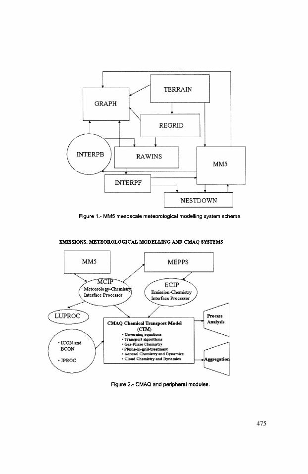
475

4. MODELLING DOMAIN DESIGN
Consequently of providing full boundary conditions in a consistent manner for the lengthof the simulation and the spatial scales we have defined an experiment as follows. Amother domain centered in 40.00°N and 3.5°W (approximately Madrid City) and 108 kmgrid cell resolution with 75 columns and 60 rows. This domain covers an important partof North of Africa reaching the North of Scandinavian Peninsula. Figure 4 shows themother and nesting domains in Lambert Conformal projection. This domain is used forMM5. The land use file is dimensioned as follows: 72 columns and 57 rows. The land usedata set is obtained from the USGS EROS Data Center from Eurasia and Africa datasetsLambert Azimuthal Equal Area Projection (optimised for Europe) with 1 km spatialresolution. This information is extracted separately and the unified file is obtained byusing ARC/INFO Geographic Information System. The resulted land use file is averagedfor 4 km spatial resolution which is the highest resolution used in nesting level 3 in thisspecific application with CMAQ. This data set is having 2000 x 1600 4 km grid cells.The final CMAQ moth domain is 68 columns and 53 rows.
The nesting level 1 for CMAQ is 42 columns and 39 rows with 36 km grid cell spatialresolution, nesting level 2 is 30 columns and 36 rows with 12 km spatial resolution andfinal nesting level 3 is located over the Madrid Community and is having 21 columns and
476
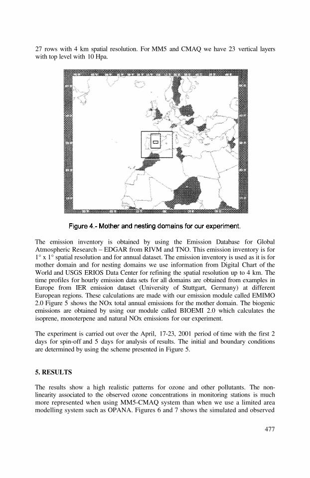
27 rows with 4 km spatial resolution. For MM5 and CMAQ we have 23 vertical layerswith top level with 10 Hpa.
The emission inventory is obtained by using the Emission Database for GlobalAtmospheric Research – EDGAR from RIVM and TNO. This emission inventory is for1° x 1° spatial resolution and for annual dataset. The emission inventory is used as it is formother domain and for nesting domains we use information from Digital Chart of theWorld and USGS ERIOS Data Center for refining the spatial resolution up to 4 km. Thetime profiles for hourly emission data sets for all domains are obtained from examples inEurope from IER emission dataset (University of Stuttgart, Germany) at differentEuropean regions. These calculations are made with our emission module called EMIMO2.0 Figure 5 shows the NOx total annual emissions for the mother domain. The biogenicemissions are obtained by using our module called BIOEMI 2.0 which calculates theisoprene, monoterpene and natural NOx emissions for our experiment.
The experiment is carried out over the April, 17-23, 2001 period of time with the first 2days for spin-off and 5 days for analysis of results. The initial and boundary conditionsare determined by using the scheme presented in Figure 5.
5. RESULTS
The results show a high realistic patterns for ozone and other pollutants. The non-linearity associated to the observed ozone concentrations in monitoring stations is muchmore represented when using MM5-CMAQ system than when we use a limited areamodelling system such as OPANA. Figures 6 and 7 shows the simulated and observed
477
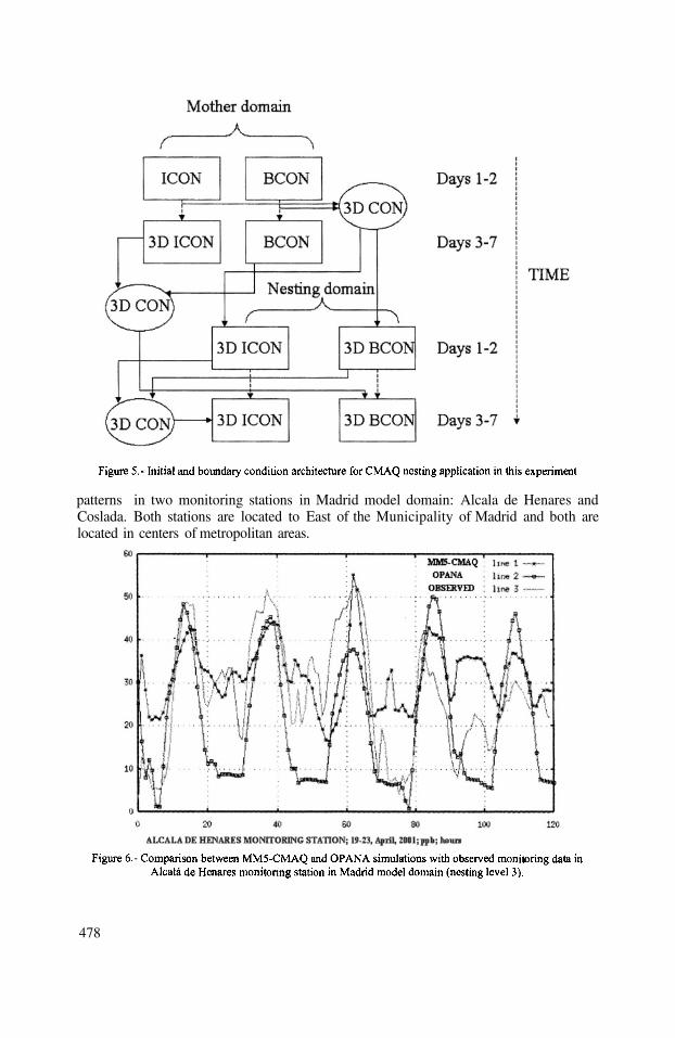
patterns in two monitoring stations in Madrid model domain: Alcala de Henares andCoslada. Both stations are located to East of the Municipality of Madrid and both arelocated in centers of metropolitan areas.
478
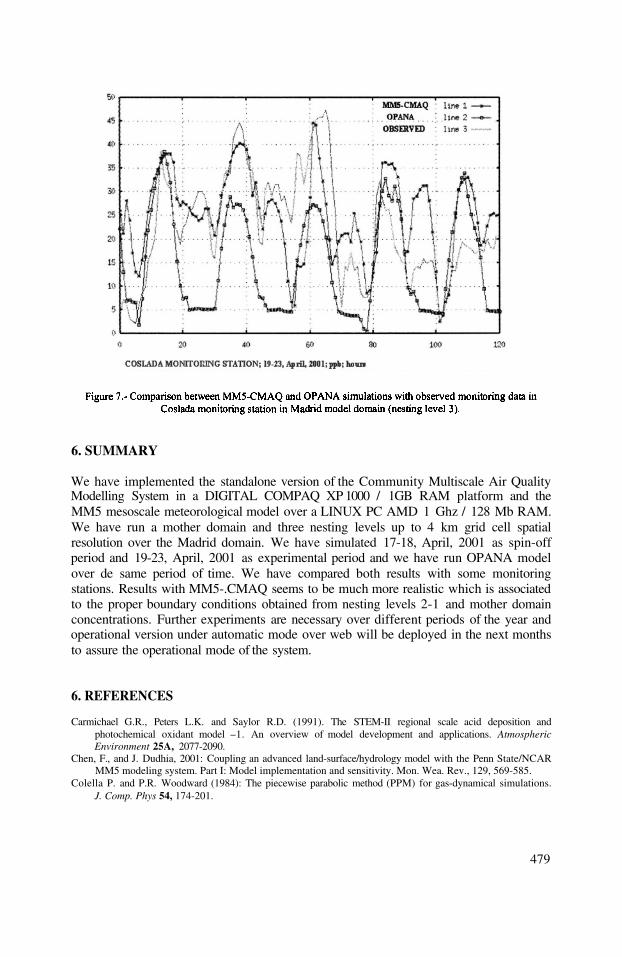
6. SUMMARY
We have implemented the standalone version of the Community Multiscale Air QualityModelling System in a DIGITAL COMPAQ XP 1000 / 1GB RAM platform and theMM5 mesoscale meteorological model over a LINUX PC AMD 1 Ghz / 128 Mb RAM.We have run a mother domain and three nesting levels up to 4 km grid cell spatialresolution over the Madrid domain. We have simulated 17-18, April, 2001 as spin-offperiod and 19-23, April, 2001 as experimental period and we have run OPANA modelover de same period of time. We have compared both results with some monitoringstations. Results with MM5-.CMAQ seems to be much more realistic which is associatedto the proper boundary conditions obtained from nesting levels 2-1 and mother domainconcentrations. Further experiments are necessary over different periods of the year andoperational version under automatic mode over web will be deployed in the next monthsto assure the operational mode of the system.
6. REFERENCES
Carmichael G.R., Peters L.K. and Saylor R.D. (1991). The STEM-II regional scale acid deposition andphotochemical oxidant model –1. An overview of model development and applications. AtmosphericEnvironment 25A, 2077-2090.
Chen, F., and J. Dudhia, 2001: Coupling an advanced land-surface/hydrology model with the Penn State/NCARMM5 modeling system. Part I: Model implementation and sensitivity. Mon. Wea. Rev., 129, 569-585.
Colella P. and P.R. Woodward (1984): The piecewise parabolic method (PPM) for gas-dynamical simulations.J. Comp. Phys 54, 174-201.
479

Flassak T. and Moussiopoulos N. (1989) Simulation of the sea breeze in Athens with an efficient non-hydrostatic mesoscale model. In: Man and his ecosystem., Vol. 3, Eds. L.J. Brasser and W.C. Mulder.Elsevier. Amsterdam. 189-195.
Ge, Xiaozhen, Li, Feng, and Ge, Ming, 1997: Numerical analysis and case experiment for forecasting capabilityby using high accuracy moisture advectional algorithm. Meteorology and Atmospheric Physics, Vienna,Austria, 63(3-4), 131-148.
Jacobson M.Z. and Turco R.P. (1994) SMVGEAR: A sparse-matrix vectorized gear code for atmosphericmodels. Atmospheric Environment, 28, 273-284.
McRae G. J. And Seinfeld J.H. (1983) Development of a second generation mathematical model for urban airpollution. II. Evaluation of model performance. Atmospheric Environment, 17, 501-522.
Peters L.K., Berkowitz C.M., Carmichael G.R., Easter R.C., Fairweather G., Ghan S.J., Hales J.M., Leung L.R.,Pennell W.R., Potra F.A., Saylor R.D. and Tsang T.T. (1995) The current state and future direction ofEulerian models in simulating the tropospheric chemistry and transport of chemical species: A review.Atmospheric Environment, 29, 2, 189-222.
San José R., Rodríguez L. And Moreno J. (1994). An application of the “Big Leaf” deposition approach to themesoscale meteorological transport and chemical modelling in a three dimensional context. Proceedingsof the EUROTRAC Symposium. Eds. Borrel P.M., Borrell P., Cvitas T. and Seiler W. 620.
San José R., Rodríguez M.A., Pelechano A. And González R.M. (1999) Sensitivity studies of dry depositionfluxes. In Measuring and Modelling Investigation of Environmental Proceses. WITpress ComputationalMechanics Publications. ISBN: 1-853125660. Ed. R. San José. 205-246.
Stensrud, D. J., J. -W. Bao, and T. T. Warner, 2000: Using initial condition and model physics perturbations inshort-range ensemble simulations of mesoscale convective systems. Mon. Wea. Rev., 128, 2077-2107.
Venkatram A. and Karamachandani P. K. (1989). The ADOM II scavenging module: incorporation of improvedcumulus cloud module. ENSR Doc. No. 0780-004-205.
Warner, T. T. and H. M. Hsu, 2000: Nested-model simulation of moist convection: The impact of coarse-gridparameterized convection on fine-grid resolved convection through lateral-boundary-condition effects.Mon. Wea. Rev., 128, 2211-2231.
480

DISCUSSION
M. ZHANG
R. SAN JOSE
D. STEYN Does your modelling system incorporate stratospheric intrusions ofozone ?
R. SAN JOSE No. It is planned to do it in the future because of the considerableimportance that that process is having in predicting ozoneconcentrations.
481
1)
2)
Do you use the same emissions inventory for different modeldomains ? If so, how do you keep emission flux conservativefor each domain ?How did you specify emission rate for the lowest model layer, asthe height of the layer in your model system changes with time ?
1)
2)
We use EDGAR emission inventory with 1x1 degree resolutionannual total data set. We use USG5 1 x 1 km land use files(AVHRR/NOAA), DCW information and world population database to assure inhomogeneity distribution of emissions by usingour EMIMO model.In this version, emissions are located at the surface since noinformation has been found related to the height of industrialchimmeneys in the original and other data bases.

This page intentionally left blank

ESTIMATES OF UNCERTAINTY IN URBAN AIRQUALITY MODEL PREDICTIONS
Sotiris Vardoulakis, Bernard Fisher, Norbert Gonzalez-Flesca, and KoulisPericleous*
The deterministic approach of running a single dispersion model using a specificinput data set of fixed values has been traditionally adopted in air quality management. Insome cases more than one model has been involved in inter-comparison studies anddifferent emissions scenarios have been taken into account in order to assess future airquality trends. However, most of the modelling work has been so far oriented towardsdeterministic simulations of ambient air pollution. This approach does not reflect theuncertainties attached to the input data, model formulation and stochastic variability ofthe atmosphere. Given the complexities of urban environments and the inherentlimitations of mathematical modelling, it is unlikely that a single model based onroutinely available meteorological and emission data will give satisfactory short-termpredictions. Moreover, deterministic air quality modelling might lead in same cases toerroneous decisions with serious financial and social implications when used forregulatory and planning purposes.
In this study, a method involving the use of more than one urban dispersion models,in association with different emission simulation methodologies and meteorological inputdata from different sources, is proposed for predicting best CO and benzene estimates,and related confidence bounds. This method was tested using experimental data obtainedduring intensive monitoring campaigns in busy street canyons in Paris, France. Threerelatively simple dispersion models (OSPM, AEOLIUS and STREET) which are likely tobe used for regulatory purposes were selected for this application. The comparisonbetween simulated and observed concentrations demonstrated the advantages andlimitations of this approach. Without resorting to sophisticated statistical techniques, this
* Sotiris Vardoulakis, Institut National de l’Environnement Industriel et des Risques (INERIS), and School ofComputing and Mathematical Science, University of Greenwich. Bernard Fisher, National Centre for RiskAnalysis & Options Appraisal, Environment Agency, 11 Tothill Street, London SW1H 9NF, UK. NorbertGonzalez-Flesca, INERIS, Parc Technologique ALATA, B.P. 2, 60550 Verneuil-en-Halatte, France. KoulisPericleous, School of Computing and Mathematical Science, University of Greenwich, Maritime GreenwichUniversity Campus, 30 Park Row, London SE10 9LS, UK.
1. INTRODUCTION
Air Pollution Modeling and Its Application XV, Edited byBorrego and Schayes, Kluwer Academic/Plenum Publishers, New York, 2002 483
study explores practical methods for quantifying and presenting model uncertainties in away that can be easily understood by local authority officers and general public.
Two comprehensive data sets were created from field experiments conducted atrepresentative street canyon sites in Paris during winter (Bd. Voltaire, December 1998)and summer (Rue de Rennes, July 1999). The two sites are busy four lane streets withlarge pavements and uniform buildings lining up continuously on both sides. The height-to-width (H/W) ratios for Bd. Voltaire and Rue de Rennes were approximately equal to0.8 and 1.1, respectively.
Traffic-related atmospheric pollutants were sampled during five and eight days inBd. Voltaire and Rue de Rennes, respectively. Continuous CO monitoring and diffusivebenzene sampling was carried out in both the canyons throughout the respectivecampaigns. The relative street and background contributions to the pollution levelsobserved on the roadside were derived from benzene measurements. The experimentallay out and monitoring results from these campaigns were presented elsewhere(Vardoulakis et al., 2001).
Synoptic wind data and other meteorological information were obtained from threepermanent monitoring stations operated by Meteo France. Two of them were located inurban settings within Paris: (a) park Montsouris, and (b) St. Jacques tower. The thirdstation was located at (c) Orly airport, in approximately 12 km distance from centralParis.
The average traffic volumes in Bd. Voltaire and Rue de Rennes duringmeasurements were 30,000 and 23,000 veh/day, respectively. Hourly traffic data wereobtained from automatic counters permanently operating in both the streets. The vehiclefleet composition was estimated from on site spot measurements during the campaigns.
The rate of release of emissions in the street was derived from traffic volumes andcomposite emission factors. Two different methods were applied for calculating COemission factors: (a) The protocol used by Buckland and Middleton (1999), and (b) theIMPACT road traffic emission model commercialised by ADEME (1998). This modeluses COPERT II methodology (Ntziachristos and Samaras, 1997) to quantify fuelconsumption and atmospheric releases of a specified vehicle fleet in a given year inFrance. The required input information includes traffic volume and composition, averagevehicle speed, and length and slope of the road segment of interest. In addition, the monthof the year is used to estimate average ambient temperatures, which are further used forcalculating evaporative and cold running emissions. The model provides default valuesfor the average travelling distance and the fraction of this distance run with a cold enginein France.
The estimated values from both the methods, were compared for consistency withCO emission factors specific to the French vehicle fleet reported in other recent studies(Touaty and Bonsang, 2000; Jones et al., 2000). All values are summarised in Table 1.
484
2. INPUT DATA

In this study, three parameterised dispersion models (STREET, OSPM, andAEOLIUS) were used to simulate pollutant dispersion within canyons. These relativelysimple codes (or variations of them) have been widely used by local authorities and airquality networks in Europe. They are likely to be involved in a variety of applicationsincluding air quality and traffic management, urban planning, population exposurestudies, etc.
Like most empirical street canyons models, they are based on the assumption that awind recirculation zone is formed within the canyon when the roof-top wind blowsperpendicularly or near-perpendicularly to the street axis (Berkowicz et al., 1997). Thisair vortex causes a downward flow of relatively clean air on the windward side of thecanyon and an upward flow of air mixed with exhaust gases on the leeward side. Thisflow gives rise to high cross-road and vertical pollution gradients in the street.
Empirical models have been proved to describe quite efficiently concentrationgradients in regular canyons, especially for the perpendicular wind situation.Nevertheless, more sophisticated modelling techniques might be needed to simulatedispersion under low wind conditions or in more complex urban environments (e.g.asymmetric and deep canyons, intersections, etc.). In these cases, the single vortexassumption does not appear realistic.
STREET and OSPM have been parameterised according to different fieldexperiments and used successfully in many scientific and engineering applications(Johnson et al., 1973; Qin and Kot, 1993; Kukkonen et al., 2001). AEOLIUS is a morerecent model based on the same formulation as OSPM and mainly used in the U.K.(Buckland, 1998).
The total uncertainty involved in modelling simulations can be considered as the sumof three components(Hanna, 1988): (a) The uncertainty due to errors in the modelphysics, (b) the uncertainty due to input data errors, (c) the uncertainty due to stochasticprocesses (e.g. turbulence) in the atmosphere.
STREET, OSPM and AEOLIUS were initially used in a traditional manner toproduce estimates of roadside CO concentrations in Bd. Voltaire and Rue de Rennes.Three independent meteorological data sets and three different emission factors (asdescribed in paragraphs 2) were used for each canyon, so as to create an ensemble set of
485
3. STREET CANYON MODELS
4. QUANTIFYING UNCERTAINTY

27 simulations for each case. It was considered that the use of different models enabledus to account, to a certain extent, for the uncertainty in model formulation. Furthermore,the use of independent wind and emission data sets was thought to represent theuncertainties due to errors in model inputs. This approach might be more realistic thandefining a priori uncertainty ranges in different input variables.
The same methodology was followed for creating ensemble sets of weekly benzeneaverages corresponding to different receptor locations in both the canyons.
For quantifying the total uncertainty in model predictions, medians together withmaximum and minimum concentrations were calculated for each set of 27 model outputscorresponding to a specific receptor location and time. The extreme concentrations werethought to bound the likely ranges of total uncertainty in the predictions. As it can beseen in Fig. 1 and 2, approximately 95% and 92% of CO observations in Rue de Rennesand Bd. Voltaire, respectively, fell within the predicted concentration ranges. In the caseof benzene, all predicted values were within the estimated error bounds (Fig. 3 and 4).
In the previous examples, the observed concentrations fell in most cases within theestimated error (or “confidence”) bounds. Nevertheless, it might be argued that theseerror limits were so large that they did not really provide any useful information. The factis that, although large uncertainties do exist, dispersion models are still used in atraditional “deterministic” way, often returning results with several significant digits. Itis, therefore, preferable to include error bounds (however large they may be) in thepredictions in order avoid inappropriate reliance on modelling results.
A more rigorous approach would require that probability functions be developed forinput and internal model parameter, and these be randomly sampled to obtain improvedensemble sets (Dabberdt and Miller, 2000). This, however, would risk to geometricallyincrease the time and consequently the cost of the simulations. It is believed thatensembles of less than 30 simulations, as shown in this study, can provide satisfactory airquality predictions and error bounds.
Model users some times assume that the total uncertainty in predictions decreases asthe complexity of the model increases. This is true only for the uncertainty attributed toerrors in the physical description of the model domain (e.g. incorrect assumptions,oversimplifications, etc.). On the other hand, sophisticated models require a largeramount of input information, which inevitably introduce a larger data uncertaintycomponent in their calculations. It is, therefore, very important to define the appropriatedegree of sophistication for a specific application, so as to achieve the lowest possiblelevel of uncertainty in modelling results.
486
5. DISCUSSION
5.1. Uncertainty in emissions
It has been suggested by other authors (Kühlwein and Friedrich, 2000) that emissionfactors represent one of the most important source of uncertainty in modelling trafficpollution. That was confirmed in the present study. CO emission factors calculated withIMPACT were 25% and 180% higher than those calculated following Buckland andMiddleton’s methodology for Rue de Rennes and Bd. Voltaire, respectively (Table 1).
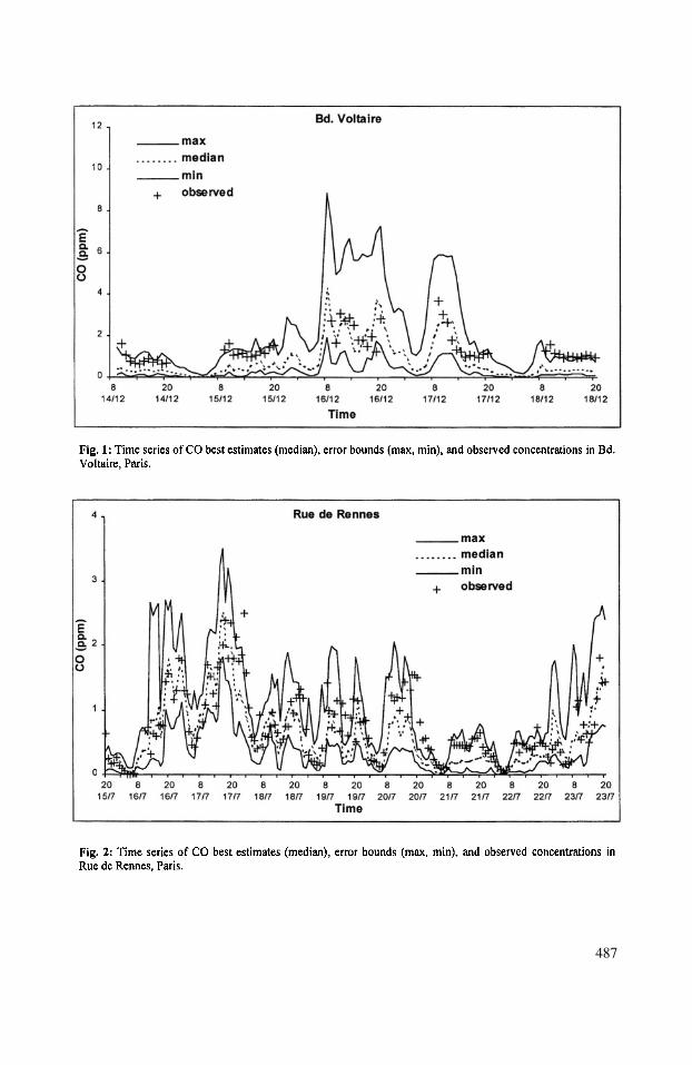
487
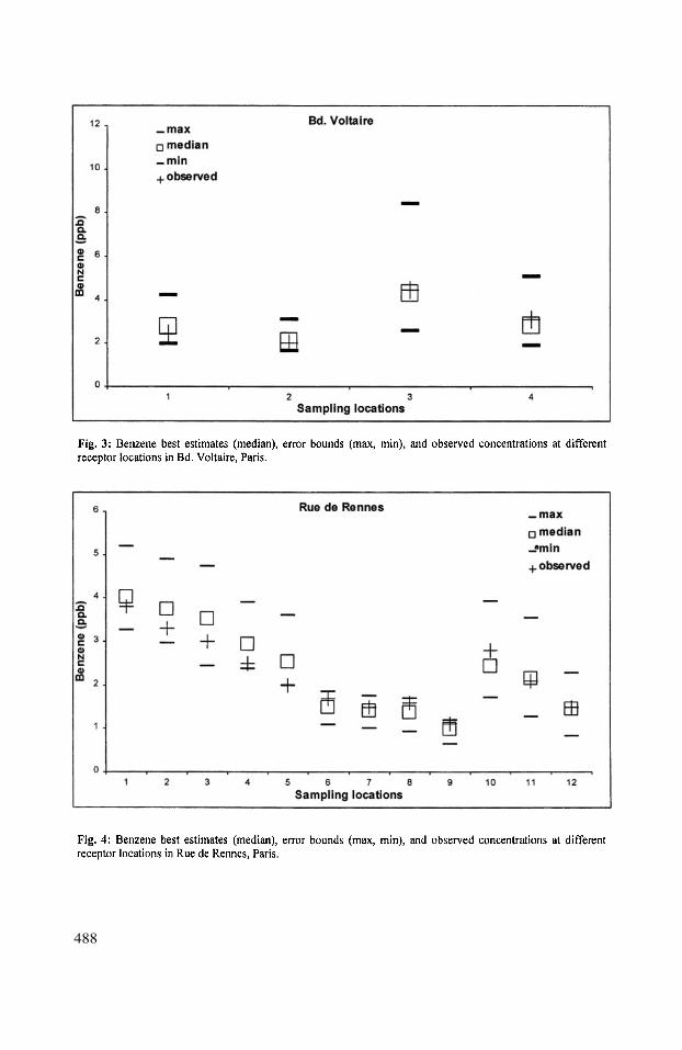
488
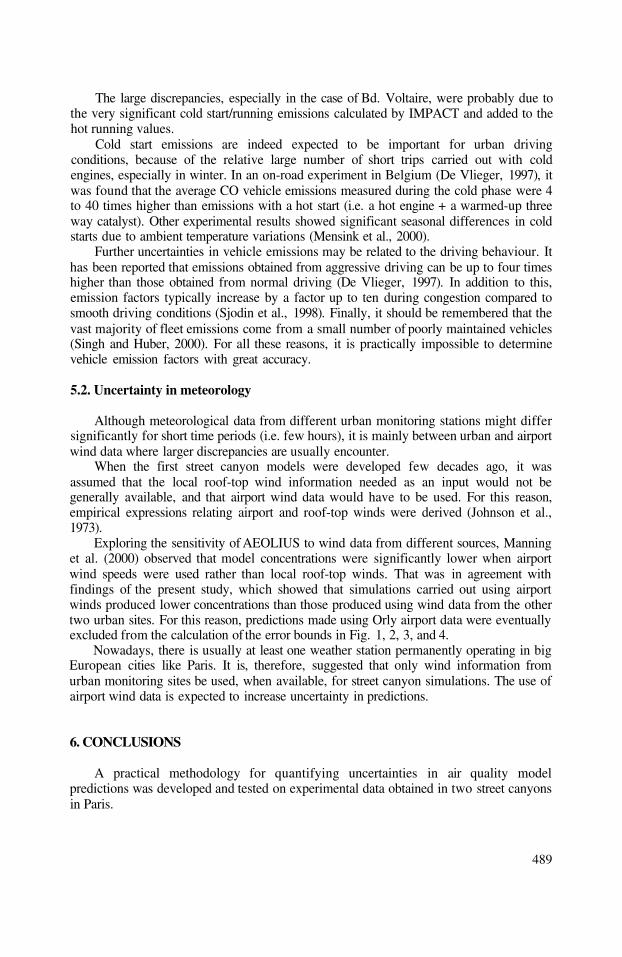
The large discrepancies, especially in the case of Bd. Voltaire, were probably due tothe very significant cold start/running emissions calculated by IMPACT and added to thehot running values.
Cold start emissions are indeed expected to be important for urban drivingconditions, because of the relative large number of short trips carried out with coldengines, especially in winter. In an on-road experiment in Belgium (De Vlieger, 1997), itwas found that the average CO vehicle emissions measured during the cold phase were 4to 40 times higher than emissions with a hot start (i.e. a hot engine + a warmed-up threeway catalyst). Other experimental results showed significant seasonal differences in coldstarts due to ambient temperature variations (Mensink et al., 2000).
Further uncertainties in vehicle emissions may be related to the driving behaviour. Ithas been reported that emissions obtained from aggressive driving can be up to four timeshigher than those obtained from normal driving (De Vlieger, 1997). In addition to this,emission factors typically increase by a factor up to ten during congestion compared tosmooth driving conditions (Sjodin et al., 1998). Finally, it should be remembered that thevast majority of fleet emissions come from a small number of poorly maintained vehicles(Singh and Huber, 2000). For all these reasons, it is practically impossible to determinevehicle emission factors with great accuracy.
A practical methodology for quantifying uncertainties in air quality modelpredictions was developed and tested on experimental data obtained in two street canyonsin Paris.
489
5.2. Uncertainty in meteorology
Although meteorological data from different urban monitoring stations might differsignificantly for short time periods (i.e. few hours), it is mainly between urban and airportwind data where larger discrepancies are usually encounter.
When the first street canyon models were developed few decades ago, it wasassumed that the local roof-top wind information needed as an input would not begenerally available, and that airport wind data would have to be used. For this reason,empirical expressions relating airport and roof-top winds were derived (Johnson et al.,1973).
Exploring the sensitivity of AEOLIUS to wind data from different sources, Manninget al. (2000) observed that model concentrations were significantly lower when airportwind speeds were used rather than local roof-top winds. That was in agreement withfindings of the present study, which showed that simulations carried out using airportwinds produced lower concentrations than those produced using wind data from the othertwo urban sites. For this reason, predictions made using Orly airport data were eventuallyexcluded from the calculation of the error bounds in Fig. 1, 2, 3, and 4.
Nowadays, there is usually at least one weather station permanently operating in bigEuropean cities like Paris. It is, therefore, suggested that only wind information fromurban monitoring sites be used, when available, for street canyon simulations. The use ofairport wind data is expected to increase uncertainty in predictions.
6. CONCLUSIONS

This method was based on the use of three different models, independentmeteorological data sets and different emission factors, for creating ensemble sets ofstreet canyon simulations. That enabled us to calculate best estimates of CO and benzeneconcentrations, and related error bounds.
It was not the intention of the authors to simulate all possible sources of uncertaintyin urban dispersion modelling. Uncertainties due to stochastic atmospheric processes ordue to errors in some of the input parameters (e.g. dimensions of the street, trafficvolumes, etc.) were not here taken into consideration. However, it is believed that theabove presented methodology strikes a reasonable balance between simplicity andreliability on urban dispersion models.
ADEME, 1998, Emissions de polluants et consommations liées à la circulacion routière, ADEME, Paris.Berkowicz R., Hertel O., Larsen S.E., Sorensen N.N., Nielsen M., 1997, Modelling traffic pollution in streets,
NERI, Roskilde, Denmark.Buckland A. T., 1998, Validation of a street canyon model in two cities, Env. Monitor. & Assess. 52: 255-267.Buckland A. T., Middleton D. R., 1999, Nomograms for calculating pollution within street canyons,
Atmospheric Environment 33: 1017-1036.Dabberdt W. F., Miller E., 2000, Uncertainty, ensembles and air quality dispersion modeling: applications and
challenges, Atmospheric Environment 34: 4667-4673.De Vlieger I., 1997, On-board emission and fuel consumption measurement campaign on petrol-driven
passenger cars, Atmospheric Environment 31: 3753-3761.Hanna S. R., 1988, Air Quality Model Evaluation and Uncertainty, J. Air Pollution Control Assoc. 38: 406-412.Johnson W. B., Ludwig F. L., Dabberdt W. F., Allen R. J., 1973, An urban diffusion simulation model for
carbon monoxide, J. Air Pollution Control Association 23: 490-498.Jones S. G., Fisher B. E. A., Gonzalez-Flesca N., Sokhi R., 2000, The use of measurement programmes and
models to assess concentrations next to major roads in urban areas, Env. Monitor. & Assess. 64: 531-547.Kühlwein J., Friedrich R., 2000, Uncertainties of modelling emissions from road transport, Atmospheric
Environment 34: 4603-4610.Kukkonen J., Valkonen E., Walden J., Koskentalo T., Aarnio P., Karppinen A., Berkowicz R., Kartastenpää R.,
2001, A measurement campaign in a street canyon in Helsinki and comparison of results with predictionsof the OSPM model, Atmospheric Environment 35: 231-243.
Manning A. J., Nicholson K. J., Middleton D. R., Rafferty S. C., 2000, Field study of wind and traffic to test astreet canyon pollution model, Env. Monitor. & Assess. 60: 283-313.
Mensink C., De Vlieger I., Nys J., 2000, An urban transport emission model for the Antwerp area, AtmosphericEnvironment 34: 4595-4602.
Ntziachristos L., Samaras Z., 1997, COPERT II: Computer programme to calculate emissions from roadtransport - User’s manual, European Environment Agency, Copenhagen.
Qin Y., Kot S. C., 1993, Dispersion of vehicular emission in street canyons, Guangzhou city, South China(P.R.C.), Atmospheric Environment 27B: 283-291.
Singh R. B., Huber A. H., 2000, Development of a microscale emission factor model for CO for predicting real-time motor vehicle emissions, J. Air Waste Manage. Assoc. 50: 1980-1991.
Sjodin A., Person K., Andreasson K., Arlander B., Galle B., 1998, On-road emission factors derived frommeasurements in a traffic tunnel, Int. J. Vehicle Design 20: 147-158.
Touaty M., Bonsang B., 2000, Hydrocarbon emissions in a highway tunnel in the Paris area, AtmosphericEnvironment 34: 985-996.
Vardoulakis S., Gonzalez-Flesca N., Fisher B. E. A., 2001, Assessment of traffic-related air pollution in twostreet canyons in Paris: implications for exposure studies, Atmospheric Environment (in the press).
490
ACKNOWLEDGEMENTS
The authors would like to thank J-C. Pinard and A. Frezier (INERIS) for theirtechnical assistance, and Dr. R. Berkowicz (NERI) for providing and discussing OSPM.
REFERENCES

In comparing the sensitivity of the different models againstobservations you do not include the experimental error bands.How would the conclusions have changed (e.g. ranges ofvariability in the input parameters) if you had included also thisexperimental variability in the comparison ?
I agree that uncertainties in measurements should be eventuallytaken into account. Nevertheless, measurement uncertainties aregenerally expected to be smaller than modelling uncertainties andfor this reason we believe that our preliminary conclusions arevalid.
491
DISCUSSION
S. RAFAILIDIS
S. VARDOULAKIS

This page intentionally left blank
Nowadays, air quality modeling has become an essential tool for determiningcompliance with regulations. Predictions made by any air quality model used in scientificstudies or in regulatory applications should be sufficiently reliable, and quality assuranceof a specific model is a pre-requisite to be able to use it with sufficient confidence.
The past ten years, model formulation has improved significantly, diminishing inthis way the influence of inherent model formulation errors (Venkatram, 1999).However, differences between model predictions and observations have not disappearedwith the diminishing of inherent model errors, which makes clear that also attentionshould be paid to the existence of data errors and their propagation through the model.Data errors often seem to be forgotten in the common belief that monitoring data are “thereal world”. As models rely upon emissions and meteorological inputs, an importantfeature for any model is accessibility to reliable input data. Often the error in thedetermination of these inputs fully justify the disagreements between predictions andobservations (Irwin, et al., 1987).
To quantify differences between model output and observations, different standardevaluation techniques have being developed the past years, as for example the ModelValidation Kit (Olesen, 1995) or the ASTM procedure (Cooper, 1999); being the first ofthese still the most widely used evaluation technique. The Model Validation Kit (MVK)is a collection of three experimental data sets accompanied by software for modelevaluation. It is a practical tool, meant to serve as a common frame of reference formodelers, although it does have well recognized limitations. In this study, the statisticalindices included in the model validation kit were analyzed in terms of error propagation.
* Ann Wellens, DEPFI-UNAM, P.O. Box 70-256, Mexico, D.F., 04510,[email protected]
EFFECTS OF INPUT DATA ERRORS ON SOMEINDICES FOR STATISTICAL MODEL EVALUATION
Ann Wellens*
1.
Air Pollution Modeling and Its Application XV, Edited byBorrego and Schayes, Kluwer Academic/Plenum Publishers, New York, 2002 493
INTRODUCTION

Relative errors are calculated in an exact way, without ignoring second order errorterms, as these can become significant when individual relative data errors are important.
Note that:
The model validation kit (MVK) uses a basic set of statistical indices that can beused to evaluate air pollution dispersion models. The included indices are the mean andstandard deviation of observed and simulated concentration values, bias and fractionalbias of the simulated concentrations, fractional standard deviation, normalized meansquare error, correlation coefficient and proportion of values that lies between a factor of2 (see for example Canepa and Builtjes, 1999).
494
2. ERROR PROPAGATION
Defining the absolute error as the difference between the exact value and itsapproximation and the relative error as the quotient of the absolute error and the truevalue, the global data error due to propagation of the individual data errors can becalculated.
Consider two numbers and where and represent theabsolute errors of numbers a and b respectively. The asterisk in a* and b* indicate thatboth numbers include an exact part (a or b) and an inherent data error and Theirrelative errors and can be found dividing the respective absolute error by the realquantity a or b, where absolute errors have the same dimension as their correspondingvariables and relative errors are expressed in percent.
The propagation of the relative numerical errors in arithmetic operations as sums,multiplications and divisions, due to errors on the operands, are found in table 1:
Propagated relative errors in addition and subtraction operations are a weightedaverage of the individual relative errors in a and b.Propagated relative errors in multiplications and divisions do not depend on thevalues of a and b, only on their individual relative errors.
3. STATISTICAL INDICES

These indices are resumed in table 2, where n is the total number of the receptors andand are respectively the observed and predicted concentration at the i-th receptor.
Their significance is explained in numerous papers and will not be repeated here.
The error propagated when calculating the average value of the observed andpredicted values equals a weighted average of the relative errors associated to theobserved or predicted concentrations at the i-th receptor.
Note that if all observations or all predicted values have respectively the same dataerror in each data point or the error propagated in the average valuewould be constant and equal:
495
4. ERROR PROPAGATION THROUGH STATISTICAL INDICES
The previously presented error propagation formulas were applied to find the relativeerror made in each of the presented statistical indices, when model results andobservations present data errors. In the following formulas, corresponds to the dataerror of observation i, while corresponds to the data error of the predicted value i.
4.1. Average Value of Observed and Predicted Concentrations, and

The errors propagated when calculating the standard deviation of the observed andpredicted values equal:
Note that when all observed or predicted values have the same error in each datapoint, Eqs. (5) and (6) reduce to:
Propagated error when calculating the bias, equals Theerror propagated when calculating the bias, is the weighted average of the propagatederrors in the mean value of observed and predicted values. Note that when the propagatederror in the mean of the observed and predicted values equal each other, the bias wouldpropagate this same error. When this is not so, and the difference between and issmall, the error propagated in the bias can become quite high.
496
4.2. Standard Deviation of Observed and Predicted Concentrations, and
and
4.3. Bias, B
4.4. Fractional Bias, FB
When calculating fractional bias, data errors propagate in the following way:
When the propagated errors in the mean of the observed and predicted values are thesame the propagated error for the fractional bias would be zero.
4.5. Fractional Standard Deviation, FS
For the fractional standard deviation, data errors propagate in the following way:

The formulas presented in the previous section are useful in sensitivity analysis,where the influence of input data errors on model evaluation results is studied. Whenerrors are propagated through statistical indices, the calculated quantity for each of them
497
When all observed and predicted values have the same error in each data point, andat the same time it would follow that and Eq. (9) reduces to zero.
4.6. Normalized Mean Squared Error, NMSE
Error propagation in the normalized mean square error equals:
When all observed and predicted values have the same error in each data point, butnot necessarily Eq. (10) reduces to zero.
4.7. Linear Correlation Coefficient, r
The error propagated when calculating the linear correlation coefficient is:
Again, when all observed and predicted values have the same error, the previousequation would reduce to 0% and the correlation coefficient would not propagate anydata error. In case the error propagated in the correlation coefficient doesonly depend on the error of and something similar would happen for propagatederrors in predicted values.
4.8. Fraction of Two, FA2
When data errors exist in observed and predicted values, factor of two will considerthe fraction of observations for which
and not the fraction for which the relationship has a value between 0.5 and 2.
5. APPLICATION OF ERROR PROPAGATION THROUGH STATISTICALINDICES

can vary significantly. This will be demonstrated by calculating the presented statisticalindices for the modeling results from the Belgian IFDM and the Rumanian Inpuffmodels, for the Copenhagen data set available through the Model Validation Kit (Olesen,1995).
Different error scenarios were studied, taking into account over- and/orunderestimation of the variable in study. For the observed values, a constant data error of10% was considered, which is consistent with data presented for concentrationmeasurements (see for example Moussiopoulos, 1999). For the predicted values, ahypothetical propagated data error of 35% was considered.
Determination of the way in which data errors propagate through mathematicalmodels was not the goal of this investigation, however, it can be stated that the relativepropagated error changes with the position vector (X, Y, Z) and depends on the modelformulation, including for example for Gaussian models (Wellens, 1999) the usedstability scheme and plume rise formulas, consideration of reflection at ground level ormixing height, wind speed determination at emission height and so on.
In this study the hypothetical value of 35% was used, although real propagated dataerror can become a lot bigger if adverse conditions are present. This error cannot beconsidered constant, exactly because it depends even on the distance from the source; forsimplification, the same quantity of 35% for all predicted values is used, but some valuesare overestimated while others are underestimated.
The used error scenarios are:
For both scenarios, all described indices were calculated; results were compared withthe indices calculated in absence of data errors. Tables 3 and 4 resume the results of thesecalculations, indicating also the relative error made for each statistical index and errorscenario, for the·IFDM and Inpuff models respectively.
Tables 3 and 4 prove numerically that data errors can propagate through statisticalindices, presenting higher or lower values than the “correct” ones, depending on the useddata set.
498
The following results are notorious:
For scenario 1, the “correct” negative biases of –80.8 (IFDM model) and –72.10(Inpuff model) convert into positive biases of 35.88 and 29.39 respectively,which corresponds to respective errors of –144.4% and –140.8% with respect tothe “correct” values. As negative values correspond to underestimation andpositive values to overestimation, this result indicates that presence of input dataerrors can change the judgment according to over- or underestimation of themodel.

For scenario 2, the negative bias values increment in respectively 144.4 and140.8 percent to –197.45 (IFDM model) and –173.59 (Inpuff model). In otherwords, considering the error propagated in this scenario, the underestimationwould be judged to me more than 2 times the “correct” value.No other scenarios are presented, but some error combinations can provide anerroneous bias value very close to zero, although the model indicates a clearunder- or overestimation when no data errors are present.In general, overestimation of the model output and/or observations does nothave the same effect on the final value of the statistical indices asunderestimation. This would only be so for so called linear indices as averagevalues and bias. In tables 3 and 4 it can be seen that the error propagated in biasand mean values is exactly the same in magnitude for both scenarios, butopposite in sign. For all other presented indices, the effect can be a lot bigger incase of overestimation that in case of underestimation, or vice versa. For
499
example, in scenario 2 the correlation coefficient was underestimated in 19.2%(IFDM) and 35.4% (Inpuff) respectively, while for scenario 1 the errorpropagated in the correlation coefficient was only 8% (IFDM) and 2.1% (Inpuff)respectively.
This paper studies the propagation of data errors in observations and model results,through statistical indices used to evaluate air dispersion models. Presented results fortwo models evaluated previously with the model evaluation kit, the Belgian IFDM modeland the Rumanian Inpuff model, indicate that statistical indices are influenced by existingdata errors. This has been corroborated for the indices proposed in the Model ValidationKit, but in fact it is valid for whatever index that can be used for the statistical evaluationfor dispersion models.
A constant error of 10% for observations was considered; for predictions, aconservative value of 35% was used, although model propagation through the differentmodels was not studied. If data errors in each of the input variables are considered,propagation through different models can also be found.
Overestimation does generally not have the same effect as underestimation.Generally one of them produces much worse results than the other one. Althoughsometimes errors are cancelled, generally the propagation is worse when individual dataerrors in observations and predicted values increase. In occasions, propagation of dataerrors can change the judgment about the performance of the model of interest. Asdifferent models propagate data errors in a different way, a model can be classified as the“worst performing” without deserving it, or the other way around.
In this paper only some results were presented, and some may seem to be onlyslightly significant. However, different data sets, models and statistical indices should bestudied to understand to which extend data errors can influence model results and evenperformance evaluation judgments.
Canepa, E. and Builtjes, P. J. H., 1999, Methodology of model testing and application to dispersionsimulation above complex terrain, International Conference on Harmonisation within AtmosphericDispersion Modelling for Regulatory Purposes, Rouen, France.
Irwin, J. S., Rao, S. T., Peterson, W. B. and Turner, D. B., 1987, Relating error bounds for maximumconcentration estimates to diffusion meteorology uncertainty, Atmos. Environment, 21 (9): 1927-1937
Moussiopoulos, N., Sahm, P., Münchow, S., Tonnesen, D. F., de Leeuw, F. and Tarrasón L., 1999,Uncertainty analysis of modeling studies included in air quality assessments. International Conference onHarmonisation within Atmospheric Dispersion Modelling for Regulatory Purposes, Rouen, France.
Olesen, H. R., 1995, Datasets and protocol for model validation kit for the workshop on operational shortrange atmospheric dispersion models for environmental impact assessments in Europe'. J. of Environment andPollution, 5(4-6): 693-701.
Venkatram, A., 1999, Applying a framework for evaluating the performance of air quality models,International Conference on Harmonisation within Atmospheric Dispersion Modelling for RegulatoryPurposes, Rouen, France.
Wellens, A., 2001, Comparison of the inherent data error in plume rise models, Int. J. Environment andPollution, in Press.
500
6. CONCLUSIONS
7. REFERENCES
DISCUSSION
1) Perhaps assuming constant relative error in observations is aninappropriate model since relative error normally increases rapidlyas one approaches the limit of detection.2) How can you identify the most sensitive variables (input) byexamining the statistically indices you displayed ?
1) In effect, relative errors in observations are not necessarilyconstant. Analysis of the measurement errors (for example increaseclose to the detection limit) was not the aim of this paper. However,it should definitely be studied, as relative errors in measurements canprovoke a in some cases quite important differences betweenpredictions and observations.
501
D. HANSEN
A. WELLENS
2) Some variables or approximations (for example: plume rise,whether or not reflection is included, etc.), may not cause bigdifferences in the predicted concentration values, and willconsequently not have a big influence on a specific statistical indexused to evaluate a certain model. On the contrary, this specific indexcould be affected very much by the existence of a relative error insome other variable (for example the gas exit temperature), whichwould produce a concentration result differing very much from the“real” estimated value that would have been calculated if the error inthis input variable would have been absent.In this case, the value of the statistical index is not reflectingdifferences between models, but sensitivity of the model and/orstatistical index to errors in the input data. As analytical propagationformulas are available, the proposed procedure can be used to learnwhich variables provoke the biggest differences in the statisticalindices used.

This page intentionally left blank

POSTER SESSION

This page intentionally left blank
ASSESSMENT OF POLLUTION IMPACT OVER TURINSUBURBAN AREA USING INTEGRATED METHODS
G. Tinarelli, S. Alessandrini, D. Anfossi, F. Pavone, S. Cuffini*
1. INTRODUCTION
Urban and suburban areas are often characterized by the presence of industrialfacilities, goods distribution systems and major roads networks. In this respect, the airpollution control over these areas is an important activity for the protection of both theenvironment and the population health. Control strategies involve the integration amongdifferent methodologies, the management and use of air quality networks, theconstruction of emission inventories, and the use of atmospheric dispersion modelingtechniques. The last two items allow to extend the information available from a localnetwork to areas not covered by the stations and to build possible future impact scenarioscaused by new installations or by alternative pollution reduction strategies
2. GENERAL DESCRIPTION OF THE ACTIVITIES
Close to the southern boundary of the city of Turin, in Northern Italy, the Province ofTurin, one of the local authorities involved in the air pollution management, has startedactivities including the development of emission inventories and the use of dispersionmodels. The overall scope of this project is to cross check the emission inventory anddispersion model reliability, comparing model simulation results with availablemeasurements. The work described here involves the verification of a modeling system inmanaging both severe pollution episodes and future emission scenarios. In this respect,two preliminary test cases have been carried out over a target area of south ofthe city of Turin. The first one is centered on the impact verification of a single industrialsource present in that area, considering in particular its odorous emissions. The secondand more complex one, is the simulation of the possible impact generated by the newwholesale agricultural market (CAAT), starting to operate on that site. This second taskinvolves the reconstruction of both the road traffic modifications and the impact of these
* G. Tinarelli, ARIANET S.r.l., viale Elvezia 42, 20052 Monza (Milano), Italy. S. Alessandrini, CESI S.p.a.,Via Reggio Emilia 39, 20039 Segrate (Milano), Italy. D. Anfossi, CNR, Istituto di Cosmogeofisica, CorsoFiume 4, 10133 Torino, Italy. F. Pavone and S. Cuffini, Provincia di Torino, Area Ambiente, Via Valeggio 5,10128 Torino, Italy
Air Pollution Modeling and Its Application XV, Edited byBorrego and Schayes, Kluwer Academic/Plenum Publishers, New York, 2002 505

modifications on the pollution levels over the whole area. The entire set of simulationshave been made by using a three dimensional modeling approach over complex terrain,that uses a diagnostic mass-consistent wind reconstruction model MINERVE coupledwith the Lagrangian particle dispersion model SPRAY version 2 (Tinarelli et al. 2000).To estimate the emission factors from road sources for the dispersion model, a programimplementing the COPERT methodology over a complex grafo has been used.
3. SUMMARY OF MAIN RESULTS
Two simulation periods, each lasting two complete days, have been chosen asrepresentative of typical meteorological conditions, potentially critical for pollutantdispersion. The first one is a summer period representing convective conditions with lightwinds blowing in a breeze regime, the second one is a winter period characterized by alow windspeed, stable condition. This choice has been made analyzing the time seriesavailable from the local anemometers of the monitoring network. Simulations of theodorous emission from the industrial source have shown a satisfactory spatialcorrespondence with the available data representing the area of the impact episodes.Dilution factors at different distances from the source have been estimated fromconcentration levels, allowing the definition of the area of potential impact around theemission point and the amount of population involved. Results from the simulation of theroad traffic impact involved the reconstruction of hourly and daily averaged CO andconcentration fields, generated by the normal traffic levels before the installation ofCAAT. These results represent the background concentration levels. A future scenarioproviding new emission factors, obtained taking into account the road traffic due to theCAAT only, has been simulated and systematic comparison with the background levelsperformed. As regards CO, the new emissions due to the presence of CAAT do notdetermine a significant impact both for hourly peak and daily average concentrationlevels. This is due to the kind of vehicles involved by CAAT, typically having Dieselengines. Concerning hourly concentration levels due to CAAT are insteadcomparable with those of the background traffic, whereas, on the contrary, dailyaverages are still substantially lower of background levels, due to the limited number ofhours involved by the traffic related to the market.
4. REFERENCES
Tinarelli G., D.Anfossi, M. Bider, E.Ferrero, S. Trini Castelli, A new high performance version of theLagrangian particle dispersion model SPRAY, some case studies, Air Pollution Modelling and itsApplications XIII, S.E. Gryning and E. Batchvarova eds., pp 499-507 (Kluwer Academic / Plenum Press,New York, 2000).
506

ASSESSING UNCONTROLLED EMISSIONS NEAR ALEAD WORKS
Guido Cosemans and Edward Roekens*
1. INTRODUCTION
The directive 96/62/EC allows, under certain conditions, for the use of airquality models for the assessment of ambient air quality. In eight monitoring sites locatednear a lead works (Figure 1) near Antwerp, Belgium, daily mean concentrations ofairborne lead are measured. This modelling study was set up in order to investigatewhether this monitoring network can be replaced in all or in part by air quality modelling.
2. THE MODELLING
Modelling is done for the two year period 1996-1997. During this period, 12metric tons of lead per year are emitted through 29 stacks of the lead works. Theseemissions, together with the heat content of the stack gasses and the stack height, areused to calculate the concentrations of lead in ambient air near the factory, using theIFDM-model1. According to these calculations, the emissions through the stackscontribute for only 6 % to the concentrations measured near the fence of the lead worksyard and for about 20 % to the concentrations measured at 4 km from the plant. The factthat emissions through the stacks contribute little to the concentrations of heavy metals inairborne dust in the neighbourhood of a non-ferrous industry, was known from an in-depth investigation near an antimony plant, conducted in 1978-1991.
It is very difficult to measure the diffuse emissions of a non-ferrous metal plant.In order to proceed with the study, reverse modelling was used to estimate the diffuselead emissions. The diffuse emissions were found to be 6 tons of lead per year. Takinginto account these diffuse emissions, the agreement between measured and IFDM-calculated two year average concentrations is good. For monitoring sites under thedominating wind direction, we find at 10 m from the fence measured and
modelled; at 250 m measured and calculated; at 600 m:measured and modelled; at 4 km : measured and
* Guido Cosemans, Flemish institute for technological research Vito, Remote Sensingand Atmospheric Processes, Boeretang 200, B 2400 Mol, Belgium.Edward Roekens, Flemish Environmental Agency (VMM), Department Networks andResearch, A. Van de Maelestraat 96, B 9320 Aalst, Belgium.
Air Pollution Modeling and Its Application XV, Edited byBorrego and Schayes, Kluwer Academic/Plenum Publishers, New York, 2002 507

modelled. At the latter site, lead emissions by traffic (not included in the calculations)were still important in 1996-1997.
A further analysis of measured and calculated daily mean concentrations(Figure 2) revealed that about 50% of the diffuse emissions are varying in timeproportional to the third power of the wind speed.
3. CONCLUSIONS
The study revealed the impact of the fugitive emissions at the lead works. Theexisting monitoring network can not be replaced by modelling only. Some monitoringsites will be needed to assess the evolution in time and space of the diffuse emissions ofairborne lead in the vicinity of the lead works.
REFERENCES
1.
2.
H. Bultynck and L. Malet, Evaluation of atmospheric dilution factors for effluents diffused from an elevatedcontinuous point source', Tellus, No. 24, pp. 445-472 (1972).
Air pollution near a non-ferrous metal industry, a comprehensive study, Volume 20 of the Final ScientificReport, National R&D Program on Environment-Air, Services of the Prime Minister, Brussels,/1982/1191/5/20 , 376 pages.
508
DESIGN FOR METEOROLOGICAL MONITORINGFOR AIR POLLUTION MODELING IN INDUSTRIAL
ZONE OF PANCEVO, BASED ON EXPERIENCESDURING BOMBING
Zoran Grsic, Predrag Milutinovic, Milena Jovasevic-Stojanovic, MarkoPopovic*
1. INTRODUCTION
Before conflict, no one environmental black spot in FRY had any appropriate airpollution monitoring system, not any local meteorological measurements. A consequencewas that local media informations about degree of dangers were confused at thebeginning of the bombing. The same situation was in Pancevo, a large industrial center ofoil, chemical and petrochemical industry. It is only 20 km away from the center ofBelgrade, the capital of FR Yugoslavia. In the industrial zone of Pancevo, only 3.5 kmfrom the center of the city, about 7000 workers are employed.When appearing of tremendous clouds over sky began every day event, municipalPancevo three weeks after starting of bombing moved action of a meteorologicalmeasured system establishing.With very limited funds, this system was realized. System was semi-automated, sopresence of an operator was necessary. This concept was effective in calm situations, butduring air-raid alarm this was not effective because everybody had to be in shelters,meteorological operator too.On the opposite side of Danube, about ten kilometers away, institute of nuclear sciences“Vinca “ is located. At the NATO/CCMS meeting in Varna, automatedmeteorological station stationed in the institute was presented. This station was aconstitutive part of defense of the institute if it would be bombed. All measured data wereon-line delivered to the civil information center of Belgrade, where set of atmospheric
*Zoran Grsic, Milena Jovasevic-Stojanovic, Institute of the Nuclear Sciences Vinca, POB522, YU-11001 Belgrade. Predrag Milutinovic, Marko Popovic, Institute of Physics,Pregrevica 118, YU-11000 Belgrade.
Air Pollution Modeling and Its Application XV, Edited byBorrego and Schayes, Kluwer Academic/Plenum Publishers, New York, 2002 509

dispersion codes was installed. Fortunately, institute was not bombed. Due to the vicinityof the institute to the industrial zone ‘Pancevo’, we were in opportunity to model airpollution distribution from the bombed industrial zone ‘Pancevo’.
2. BIG CHEMICAL ACCIDENTS IN INDUSTRIAL ZONE OF PANCEVO ONAPRIL 1999
On April 1999 at GET, Pancevos industrial zone was hardly bombed. Thatwasn’t the first bombing of the industrial area of Pancevo, but it was the most severe airstrike. That night factories in Pancevos industrial zone were hit by six missiles, whichdestroyed The Oil Refinery (petrol and diesel), The Petrochemical Complex (chlorine,vinyl-chloride-monomer, ethylene and HIP Azotara Fertilizer Co., (ammonia, NPK,fertilizer tanks). The bombing caused explosions and fires, as well as a release of hugequantities of hazardous substances in the surrounding area and emissions of toxic gases inthe air.It was reported that during bombing of the petrochemical complex in Pancevo about 20tones of chlorine was released from damaged tank (250 tons capacity) and 440 tons ofvinyl chloride monomer (VCM) burned out from spherical VCM tanks (1500 tonscapacity) and rail loading ramp of VCM with six train-cisterns. At the same time storagetanks were damaged in neighbor fertilizer factory and in oil refinery.A direct hit on the ethylene dichloride (EDC) storage’s of 1800 tons and a loss of 1400tons of liquid. Damage of the ammonia storage of the capacity of 15000 tons. Damage ofthe tank of hydrochloric acid (33%) and the loss of 800 tons of liquid. The storage ofnatrium-hidroxide, of the capacity of 12000 tons was hit. About 3000 tons of liquidpoured out into the Danube, A direct shot on the factory of chloralcalic electrolysis, withabout 100 tons of mercury, which contaminated the soil.Detailed meteorological situation, recorded with automated meteorological station in theinstitute “Vinca”, shaw that, from the point of view of air pollution transport, situationwas very complicated in the first 30 minutes after industrial zone Pancevo was bombedon that April 18, i.e. average 10 minutes wind direction three times was dramaticallychanged. In the moment of attack wind direction was WNW, after 10 minutes WSW andthan ENE. For the local conditions it was of the mostly importance, especially becauseonly few minutes after bombing fire companies and engines and the other persons were inthe middle of the tremendous air pollution plumes. It was very important for themodeling of transboundary transport of air pollution too, because input parameters, whichrelate to the source characteristics, are strongly determined with local meteorologicalconditions.The movement of polluted air in the area between Pancevo and Belgrade threatened toprovoke the poisoning of inhabitants of Pancevo, Belgrade, and particularly it’s northeastsuburbs, and villages. About 40000 inhabitants of Pancevo were evacuated from city.
3. AD HOC METEOROLOGICAL STATION
Solitaire of the municipal Pancevo, in the center of the city Pancevo, was promoted inmeteorological tower! Wind speed and direction sensors were mounted on tenth floor.Air temperature and humidity sensors were mounted on some the other floors. And that
510

was all of local meteorology during these the biggest chemical accidents. Relationbetween dimension of the accident and meteorological measurement obviously wasdeeply unequal.
4. EXPERIENCES AFTER BOMBING
Our assessments were that any war activities in the vicinity of the institute could causepanic if there would be lack of information. So one of the first thing we had to do was tosupply civil information center of Belgrade with prompt information about level ofcontamination and moving of the radioactive clouds if they would be formed.Meteorological monitoring based on the concept presented at the NATO/CCMSmeeting in Varna, could solve some possible problems about air pollution transport anddiffusion if the institute would be hit, but war conditions with electric power plantstemporary disabled, forced additional requirements special about continuous powersupply and on-line transfer data to the civil information center of Belgrade.In peaceful times all levels of thinking are at least one order lower than in war times, sosome solutions we had make in the past, before bombing, we had to adapt to the wardemands. To illustrate this, during bombing appeared problem what will we do if ourmeteorological tower or meteorological room would be hit. We had to make reservesolution, and it was classical meteorological station with appropriate crew, dislocatedfrom the institute location, but relatively close to the institute location.After 77 days bombing, resume is that automated station had only several interruptions,when interruption of the power supply was 30 hours longer, and once duringthunderstorm. Institute was not bombed, but the nearest distance where dropped bombwas 200-300m far from the fence of the institute, i.e. about one kilometer far from thereactor.
5. CONCLUSION
All characteristics of Vincas meteorological monitoring concept we checked in the worstpossible situations while bombs dropped, and tremendous polluted clouds covered thewhole sky, but it is an extraordinary experience.On these experiences we proposed project of automated meteorological station located atthe representative location in industrial zone Pancevo, similar to the automatedmeteorological station of the nuclear institute “Vinca”. The project is in progress.
ReferenceGrsic Z., Milutinovic P.: Automated meteorological station and appropriate software forair pollution distribution assessment, Air pollution Modeling and Its Application XIII,edited by S.-E. Gryning and E.Batchvarova, Kluwer Academic/Plenum Publishers, 2000,pp.781-782.Grsic Z., Milutinovic P., Jovasevic-Stojanovic M.: Some results of the meteorologicalmonitoring and modeling activities, in the nuclear institute “Vinca”, during the recentNATO bombing. V Intern. Symp. and Exib. on Environm. Contam. in Central andEastern Europe. Prague 2000. In press.
511

This page intentionally left blank
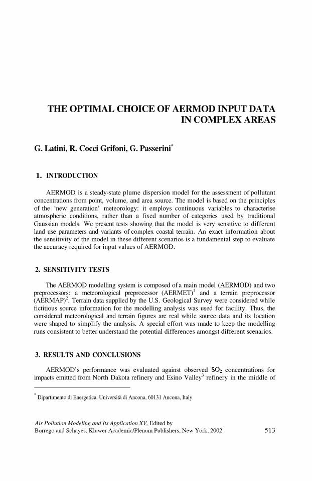
THE OPTIMAL CHOICE OF AERMOD INPUT DATAIN COMPLEX AREAS
G. Latini, R. Cocci Grifoni, G. Passerini*
1. INTRODUCTION
AERMOD is a steady-state plume dispersion model for the assessment of pollutantconcentrations from point, volume, and area source. The model is based on the principlesof the ‘new generation’ meteorology: it employs continuous variables to characteriseatmospheric conditions, rather than a fixed number of categories used by traditionalGaussian models. We present tests showing that the model is very sensitive to differentland use parameters and variants of complex coastal terrain. An exact information aboutthe sensitivity of the model in these different scenarios is a fundamental step to evaluatethe accuracy required for input values of AERMOD.
2. SENSITIVITY TESTS
The AERMOD modelling system is composed of a main model (AERMOD) and twopreprocessors: a meteorological preprocessor (AERMET)1 and a terrain preprocessor(AERMAP)2. Terrain data supplied by the U.S. Geological Survey were considered whilefictitious source information for the modelling analysis was used for facility. Thus, theconsidered meteorological and terrain figures are real while source data and its locationwere shaped to simplify the analysis. A special effort was made to keep the modellingruns consistent to better understand the potential differences amongst different scenarios.
3. RESULTS AND CONCLUSIONS
AERMOD’s performance was evaluated against observed concentrations forimpacts emitted from North Dakota refinery and Esino Valley3 refinery in the middle of
* Dipartimento di Energetica, Università di Ancona, 60131 Ancona, Italy
Air Pollution Modeling and Its Application XV, Edited byBorrego and Schayes, Kluwer Academic/Plenum Publishers, New York, 2002 513
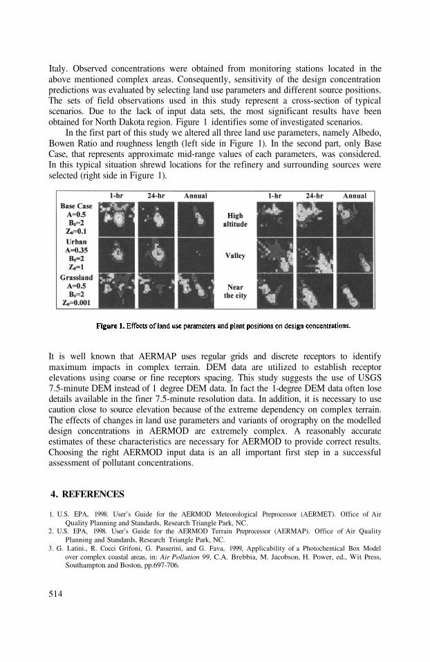
Italy. Observed concentrations were obtained from monitoring stations located in theabove mentioned complex areas. Consequently, sensitivity of the design concentrationpredictions was evaluated by selecting land use parameters and different source positions.The sets of field observations used in this study represent a cross-section of typicalscenarios. Due to the lack of input data sets, the most significant results have beenobtained for North Dakota region. Figure 1 identifies some of investigated scenarios.
In the first part of this study we altered all three land use parameters, namely Albedo,Bowen Ratio and roughness length (left side in Figure 1). In the second part, only BaseCase, that represents approximate mid-range values of each parameters, was considered.In this typical situation shrewd locations for the refinery and surrounding sources wereselected (right side in Figure 1).
It is well known that AERMAP uses regular grids and discrete receptors to identifymaximum impacts in complex terrain. DEM data are utilized to establish receptorelevations using coarse or fine receptors spacing. This study suggests the use of USGS7.5-minute DEM instead of 1 degree DEM data. In fact the 1-degree DEM data often losedetails available in the finer 7.5-minute resolution data. In addition, it is necessary to usecaution close to source elevation because of the extreme dependency on complex terrain.The effects of changes in land use parameters and variants of orography on the modelleddesign concentrations in AERMOD are extremely complex. A reasonably accurateestimates of these characteristics are necessary for AERMOD to provide correct results.Choosing the right AERMOD input data is an all important first step in a successfulassessment of pollutant concentrations.
4.
1.
2.
3.
U.S. EPA, 1998. User’s Guide for the AERMOD Meteorological Preprocessor (AERMET). Office of AirQuality Planning and Standards, Research Triangle Park, NC.
U.S. EPA, 1998. User’s Guide for the AERMOD Terrain Preprocessor (AERMAP). Office of Air QualityPlanning and Standards, Research Triangle Park, NC.
G. Latini., R. Cocci Grifoni, G. Passerini, and G. Fava, 1999, Applicability of a Photochemical Box Modelover complex coastal areas, in: Air Pollution 99, C.A. Brebbia, M. Jacobson, H. Power, ed., Wit Press,Southampton and Boston, pp.697-706.
514
REFERENCES

THE BLACK TRIANGLE AREA – FIT FOR EUROPE?
Numerical Air Quality Studies for the Black Triangle Area
Eberhard Renner, Wolfgang Schröder, Detlef Theiss and Ralf WolkeInstitute for Tropospheric Research, Leipzig, Germany
1. INTRODUCTION
The ”Black Triangle” area (covering Northern Bohemia, Southern Saxony and part ofLower Silesia) has been one of the most polluted areas in Central Europe. The mainsources of air pollution in the Black Triangle region were the emissions of sulfur and dustby power plants, industrial facilities, residential houses heating units, which were usinglignite as fuel, and road traffic. After the political changes at the end of the eighties theregion was financially supported by the European Commission to reduce the amount ofair pollution. Owing to a substantial effort of the governments of Czech Republic,Germany and Poland as well as of industry a significant improvement of air quality hasbeen achieved up to day. This has resulted mainly in a dramatic reduction of sulfur anddust emissions in this region. Unfortunately, this declining trend can not be seenconcerning the nitrogen emissions. The nitrogen emissions are increasing mainly as aresult of increasing traffic. Nitrogen oxide plays an important role in atmosphericchemistry. It produces tropospheric ozone by photochemical reactions in the presence ofvolatile organic compounds (VOC).
As a consequence, most likely we will not have a ”sulfur problem” in the future, but
we will have to demand our attention to the photooxidants, especially ozone. Thesechanges in air pollution have been investigated. With special focus on the situation inSaxony, the species sulfur dioxide, ozone, and aerosol particles have been studied. Themodel results have been evaluated for the general pollutant situation for past (1996; Thewinter 95/96 was the last ”London smog” episode in this region.), present (1998) andfuture (2005) emission scenarios. Relevant limit values for protection of human healthdefined or suggested in directives by the European Commission were checked in worstcase scenarios for the year 2005. A summary of the results of the modelling work withinthe research program OMKAS (Optimization of Emission Reduction and Control of AirPollution for the Border-Region of Saxony), funded by the Ministry of Environment ofSaxony and the European Commission, is given.
Air Pollution Modeling and Its Application XV, Edited byBorrego and Schayes, Kluwer Academic/Plenum Publishers, New York, 2002 515

2. MODEL SYSTEM AND SIMULATION SETUP
The studies are performed by utilizing the coupled mesoscale model systemMETRAS-MUSCAT. METRAS is a three-dimensional nonhydrostatic meteorologicalmodel. MUSCAT is a multiscale three-dimensional chemistry transport model, which wasdeveloped by Knoth and Wolke. It has an online coupling to METRAS. For the estimationof ozone concentrations the gas phase mechanism Euro-RADM is used. For simulation ofaerosol dynamical processes the modal model MADMAcS I has been included inMUSCAT. For the application presented on the poster two modes of particles with meanradii of for the PM 2.5 fraction and for the PM 10 fraction are considered.Only transport of primary emitted
”inert” particulate matter has been simulated as well as
coagulation, deposition and sedimentation of these particles. Formation of secondaryparticles are not considered.
High values of and particle concentrations typically occur in the model domainby winter high pressure conditions with a strong inversion and moderate winds from theeast. Summer smog with high ozone concentrations can be expected during high pressureconditions on hot summer days. Typical realistic meteorological conditions for such caseswere introduced in a conceptual way, to simulate ”worst case scenarios” for summer andwinter. In this manner the results of the second day of two days simulations can bechecked against short-time (8-hour resp. 24-hour mean) limit values for the protection ofhuman health given by relevant EU-guidelines. The simulations are not qualified toestimated annual limit values for the protection of ecosystems.
3. RESULTS
One can sum up the results as follows:
The reduction of sulfur dioxide emissions was up to now and will be mosteffective on the improvement of air quality. The concentrations of sulfur dioxidewill not exceed the relevant EU-limit values for human health.From predictions of the concentration of aerosol particles for 2005 it can beconcluded that the relevant EU-limit value for PM 10 mass concentrations will befulfilled at this time. However, these results are a preliminary estimate. There arestill a lot of subjects to be discussed in the future, like the uncertainties of particleemissions (amount and size distribution), the influence of the chemicalcomposition of the particles and the formation of secondary organic andinorganic aerosol particles by nucleation and condensation.The present and future reduction of local emissions in the modelling area itselfhas only a small effect on lowering ozone concentrations. Assuming thebackground concentrations of ozone are on the present european levelfurthermore, the simulations for the emission scenario 2005 in the model domainshow nearly the same exceedances of the suggested EU-limit values for ozone aspresent. The EU-guideline will probably be met only for lower backgroundvalues. This leads to the - well known - conclusion that emission reductionstrategies have to be performed on a larger, at least the European scale.The answer on the question ”The Black Triangle Area – Fit for Europe?“ is YES!The remaining air pollution problems are more or less the same like in the otherEU-countries and can be solved only by their joint efforts!
516
SURFACE LAYER TURBULENCE DURING THETOTAL SOLAR ECLIPSE OF 11 AUGUST 1999
Guy Schayes+, Jean-Luc Mélice* and Valérie Dulière+
1. INTRODUCTION
Total solar eclipses are not frequent events although they are not rare. Clearly no effecton air pollution is expected but we expect that the sudden reduction of solar radiation willinfluence on the atmospheric boundary layer. The decay of radiative forcing during theocculting phase of an eclipse is about 4 to 5 times more rapid than during a normalsunset. It is thus interesting to look at the atmospheric reactions in this unusualcircumstance.
Frequently, standard meteorological observations are made during these events like airtemperature, humidity or wind speed. However to our knowledge, an experimentmeasuring the air turbulence was never conducted during a total eclipse, maybe for thesimple reason that such an event rarely traverses a region where these measurements areeasily available without moving adequate equipment for long distances.
2. THE DATA
The total eclipse of 11 August 1999 traversed a line through Northern France andSouthern Belgium. Unfortunately the weather was not optimum for this observation butthe effects are still clearly visible. About five hours of measurements (resolved at onesecond) are available for the 3 wind components, the temperature and a few otheradditional measurements.
The effect of the eclipse is clearly visible on* the temperature record. Despite the fact ofthe variable cloudiness, the first temperature maximum (before totality) of 16.6°C falls to13.8 some 20 minutes after totality, and a second maximum of 17.3 around the time ofthe last contact (a thick cloud cover came then and the temperature started to drop again
+Institut d’Astronomie et de Géophysique G. Lemaître, UCL, B-1348 Louvain-la-Neuve, Belgium*IRD, Laboratoire d’Océanographie Dynamique et de Climatologie, UPMC, F-75005 Paris, France
Air Pollution Modeling and Its Application XV, Edited byBorrego and Schayes, Kluwer Academic/Plenum Publishers, New York, 2002 517
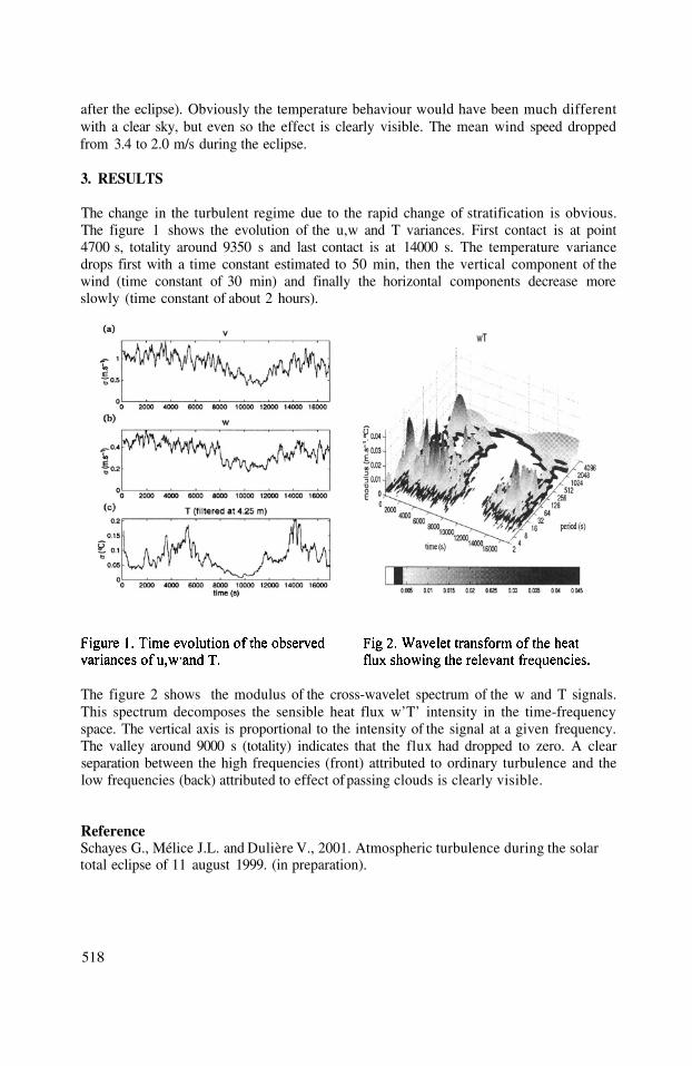
after the eclipse). Obviously the temperature behaviour would have been much differentwith a clear sky, but even so the effect is clearly visible. The mean wind speed droppedfrom 3.4 to 2.0 m/s during the eclipse.
3. RESULTS
The change in the turbulent regime due to the rapid change of stratification is obvious.The figure 1 shows the evolution of the u,w and T variances. First contact is at point4700 s, totality around 9350 s and last contact is at 14000 s. The temperature variancedrops first with a time constant estimated to 50 min, then the vertical component of thewind (time constant of 30 min) and finally the horizontal components decrease moreslowly (time constant of about 2 hours).
The figure 2 shows the modulus of the cross-wavelet spectrum of the w and T signals.This spectrum decomposes the sensible heat flux w’T’ intensity in the time-frequencyspace. The vertical axis is proportional to the intensity of the signal at a given frequency.The valley around 9000 s (totality) indicates that the flux had dropped to zero. A clearseparation between the high frequencies (front) attributed to ordinary turbulence and thelow frequencies (back) attributed to effect of passing clouds is clearly visible.
ReferenceSchayes G., Mélice J.L. and Dulière V., 2001. Atmospheric turbulence during the solartotal eclipse of 11 august 1999. (in preparation).
518

SEASONAL SIMULATION OF THE AIR QUALITY IN EAST ASIAUSING CMAQ
Seiji Sugata*
1. INTRODUCTION
Importance of long-term air quality simulation has grown to understand long-termchange of the air quality, such as, the impact of climate change. This study attempts toaddress a challenge for improvement of capability of an air quality modeling system,CMAQ (Community Multiscale Air Quality) modeling system with RAMS (RegionalAtmospheric Modeling system) to achieve long-term simulation. Results will be evaluatedby comparing with observations.
2. CONFIGURATION
A modeling system used in this study is the CMAQ modeling system modified forlinkage with RAMS meteorological data (Sugata et al., 2001, hereafter SBU2001, Byun andChing, 1999). Except for a minor change in the CTM code to update gas-phasereaction, same options and configurations as SBU2001 were used for running RAMS andCMAQ. The modeling system was run for half year from 27 December 1996 to 31 June1997. RAMS was run by continuous six times one month run with historical restart andCMAQ was run by continuous twelve times half month run with historical restart. ECMWFdata was used for RAMS assimilation.
Emission data for the simulation has been updated from the one in SBU2001 withZhang (2001), which archives sophisticatedly emission data from some projects, such asGEIA, EDGAR, and ACE-Asia/TRACE-P.
3. RESULTS
Time series of meteorological fields simulated by RAMS are compared withobservational ones at two site in Japan, where RAMS data is at the first layer of the model,about 50m, and observational data are hourly ones at the surface. One site is Osaka, whichis the second largest city in Japan, and the other is Matsue, which is along the coast to
*Seiji Sugata, National Institute for Environmental Studies, Tsukuba, Ibaraki 305-0053,
Japan
Air Pollution Modeling and Its Application XV, Edited byBorrego and Schayes, Kluwer Academic/Plenum Publishers, New York, 2002 519

Japan Sea and is supposed as an semi-urban-rural area. Long-term variations (week-to-week, seasonal) of temperature are essentially well reproduced at both sites (Figure 1.,Osaka), while shorter-term variations show some small differences. Variations of windspeed are also compared with observations and they are generally well simulated althoughthe speed is underestimated at Osaka. With considering RAMS data are come from 80kmmesh data and observational data are come from hourly surface observations independentfrom the ECMWF data used for assimilation, we can say meteorological fields are wellreproduced for long period by RAMS.CMAQ results are also compared with observational ones at the two sites. Most specieshave tendency to be underestimated compared to observation. One possible reason isemission problem.
4. SUMMARY
We have presented simulation results of RAMS/CMAQ system applied to East Asiafor half year. The meteorological results were reasonable for whole the period comparedwith observations. Further evaluation is needed for air quality modeling results.
REFERENCE
Byun, D.W. and J.K.S. Ching, ed., 1999, Science Algorithms of the EPA Models-3 Community Multi-scale AirQuality (CMAQ) Modeling System, NERL, Research Triangle Park, NC. [Available from NationalExposure Research Laboratory, U.S. Environmental Protection Agency, Research Triangle park, NC27711]
Sugata, S., D. Byun, I. Uno, Simulation of sulfate aerosol in East Asia using Models-3/CMAQ with RAMSmeteorological data, Air Pollution Modeling and its Application XIV, Gryning and Schiermeier eds.,267-275,. 2001
Zhang, M, 2001, (private communication)
520

THE ROLE OF ENERGY SOURCES OF DIFFERENTTYPES IN ATMOSPHERIC POLLUTION AND HEAT
SUPPLY OPTIONS IN IRKUTSK CITY
The structure of energy (heat) sources making up the heating system of Irkutsk cityis typical of old Siberian cities, which became industrial centres in the XX century. Thehigh fraction of small-capacity sources, including large number of household stoves ispeculiar for such cities. The installed capacity of stoves is 30% of the overall, while theirfuel consumption is 8.5% only. 76% of boiler houses have unit capacity less than 5 MW;they use mostly fixed-bed combustion. One more feature of Irkutsk heating system is thelarge fraction of coal in the fuel balance: in Irkutsk it comprises 80%, while in theEuropean Russia natural gas constitutes the major fraction.
According to the existing practice the emission factors of heat sources aredetermined mostly using computational technique and for the small sources they are oftenconsiderably underestimated. In order to reveal the actual emission factors of small heatsources we performed a series of measurements at operated boilers and stoves (Table 1).In order to disclose the most important factors causing the deviation of actual emissionfactors from the designed values we carried out a series of comparative combustion of anumber of Siberian coals under a wide range of combustion conditions (Filippov S.P. etal, 1999). It was shown that the proper operation of boilers and stoves can result in anappreciable decrease in emissions of products of incomplete burning like CO, soot, andPAH. The study of sulphurous substances emission is complicated by high variability oftheir composition. The fraction of initial coal sulphur emitted in the form of variesfrom 30 to 85% depending on the quality of burning operation.
The atmospheric dispersion of emissions over the city has been studied using thestandard model ISC3 developed by US EPA. The requirements to a model for analysis ofheating systems and the applicability of ISC3 for such studies in Siberia are discussed byKeiko et al (1999) and Keiko et al (2000). The considered emission sources includeNovo-Irkutsk CHP plant (2 point sources), organic fuel-fired boiler houses (250 pointsources), areas of residential combustion (11 area sources), and 5 CHP-plants outsideIrkutsk (12 point sources). These sources are broken into five groups according to thecombustion technology and capacity (Table 2). Some results of model study are
*Energy Systems Institute, Russian Academy of Sciences. 130, Lermontov Rd., Irkutsk 664033 Russia
Sergei P. Filippov and Alexandra V. Keiko*
Air Pollution Modeling and Its Application XV, Edited byBorrego and Schayes, Kluwer Academic/Plenum Publishers, New York, 2002 521
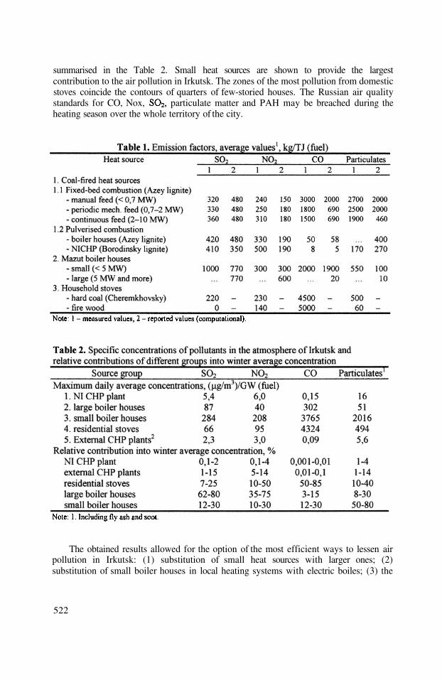
summarised in the Table 2. Small heat sources are shown to provide the largestcontribution to the air pollution in Irkutsk. The zones of the most pollution from domesticstoves coincide the contours of quarters of few-storied houses. The Russian air qualitystandards for CO, Nox, particulate matter and PAH may be breached during theheating season over the whole territory of the city.
The obtained results allowed for the option of the most efficient ways to lessen airpollution in Irkutsk: (1) substitution of small heat sources with larger ones; (2)substitution of small boiler houses in local heating systems with electric boiles; (3) the
522
change of individual houses from residential burning to electric heating; and (4) betteringthe structure of fuel consumption.
On the base of the above analyses there have been formulated and studied fifteenscenarios of the development of heating system in Irkutsk. They represent hypotheticalmarginal variants and allow the limits of air quality control to be revealed. Beside theenvironmental consideration the actual scenario of the heating system development willaccount for economical and resource factors and will be an intermediate scenario withrespect to those considered. It is shown that a change in the fuel consumption structuremay result in two-fold decrease in concentrations of sulphur dioxide and particulatematter compared with the modern case. The priority is to be given to Tugnuy andBorodinsky coals while the use of Mugun and Cheremkhovsky coals causes a rise ofconcentrations. The change of large heat sources from coal to gas does not lead to aconsiderable improvement in air quality because the largest contribution into atmosphericpollution is made by those of small capacity.
Filippov S.P., Pavlov P.P., Keiko A.V., 1999, Environmental characteristics of small-capacity heat sources.Energy Systems Institute, RAS, Irkutsk. 46 p. (In Russian)
Keiko A.V., Kuchmenko E.V., Filippov S.P., Pavlov P.P., 1999, Modelling the air quality impact of energyproduction. Energy Systems Institute, RAS, Irkutsk. 44 p. (In Russian)
Keiko A.V., Filippov S.P., Pavlov P.P., 2000, On the methods of the evaluation of air quality impact of energyproduction. Geogr. Naural. Resources, 1, pp.127-132. (In Russian)
523
REFERENCES

This page intentionally left blank
TRANSPORT SENSITIVITY ANALYSIS ON OZONECONCENTRATIONS IN IBERIAN PENINSULA BY
USING MM5-CMAQ MODELLING SYSTEM
R. San José, J. L. Pérez, I. Salas* and R.M. González**
In the last decades the interest for investigating the ozone concentrations in theatmosphere in the tropospheric layer has increased extraordinary. The ozone species isrecognized as one of the most important oxidants in the atmosphere and also as a toxicpollutant since the health consequences in human beings when high concentrations arepresent are important. It is also a greenhouse gas so that important climatic consequencesare also derived from those high concentrations. Tropospheric ozone is formed by thechemical reactions in the atmosphere when NOx and VOC’s are present and activateddepending the pressure, temperature and solar radiation. Vehicle traffic in urban and ruralareas is important. In Spain more than 25000000 and in the Iberian Peninsula is morethan 32000000. The local impact of the NOx and VOC’s emissions on ozone productionare being investigated intensively in the last decades. Little attention has been put onlarger domains and the possible impact of the total ozone tropospheric budget. Thiscontribution shows the impact on ozone total budgets of traffic emissions over the IberianPeninsula. Results show that for the first day of simulation an increase up to 25% ofozone is found and for the rest of the days of simulation increase values ranging between2 – 5 % are found. Although the 25 % increase cannot be neglected as a whole the impactover the total tropospheric ozone budget is limited. Additional experiments over severalmore different periods over the year are necessary for more conclusive results.
* Environmental Software and modelling Group, Computer Science School, TechnicalUniversity of Madrid (UPM) (Spain), Campus de Montegancedo, Boadilla del Monte28660 Madrid (Spain) http://artico.lma.fi.upm.es.** Department of Geophysics and Meteorology, Faculty of Physics, UniversidadComplutense de Madrid (Spain).
1. INTRODUCTION
Air Pollution Modeling and Its Application XV, Edited byBorrego and Schayes, Kluwer Academic/Plenum Publishers, New York, 2002 525

In this contribution we have used the MM5 model and the CommunityMuiltiscale Air Quality Modelling System (CMAQ) as representative of the thirdgeneration of Air Quality Modelling Tools to simulate the air quality concentrations overa selected period in April, 2001 over the Iberian Peninsula to understand the impact oftraffic emissions over the ozone concentrations.
The PSU/NCAR mesoscale model is a limited-area, nonhydrostatic orhydrostatic (Version 2 only),terrain-following sigma-coordinate model designed tosimulate or predict mesoscale and regional-scale atmospheric circulation. It has beendeveloped at Penn State and NCAR as a community mesoscale model and iscontinuously being improved by contributions from users at several universities andgovernment laboratories.
The Community Multiscale Air Quality Modelling System (CMAQ) and theperipheral modules are illustrated in Figure 2. We have selected for this simulation thepiece parabolic method (PPM) Colella and Woodward (1984). The updated version of theCBM-IV mechanism (36 species, 94 reactions including 11 photolytic reactions) with theisoprene chemistry mechanism and the Arrhenius type rate constant expressions. Wehave also used aerosol formation processes and aqueous chemistry. Finally we have usedthe Modified Euler Backward Iterative (MEBI) Solver which is mechanism dependentbut it isat least as precise as the QSSA but the computing time required is much lower.
We have used a mother domain of about 8100 km x 6480 km with 108 km gridcell resolution centered over the Iberian Peninsula and three different nesting levels up to4 km grid cell resolution with a domain of 108 km x 84 km over the Madrid City. Nestinglevel 2 is the Iberian Peninsula domain with 32 km grid cell resolution. For nestinglevels 1 and 2 the impact on the first day is about 25 % on the maximum levels and thisimpact is increased for nesting level 3 (since the urban emission becomes more importantin relation to the total of the model domain). The consequence of these results is that thebiogenic emissions (NOx from agricultural areas and VOC’s from forest areas) play acrucial role on the total budget of tropospheric ozone formation particularly when largeareas are considered.
526
2. THE MM5-CMAQ SYSTEM
3. APPROACH AND RESULTS

DEVELOPMENT OF THE EMISSION INVENTORYSYSTEM FOR SUPPORTING TRACE-P AND ACE-ASIA
FIELD EXPERIMENTS
New emission inventories were developed in support of the Aerosol CharacterizationExperiments(ACE)-Asia and Transport and Chemical Evolution over the Pacific(TRACE-P) experiments work on. We combine our inventories into the ACCESS(Ace-Asia and Trace-P Modeling and Emission Support System) for more integrated supportfor these two field studies. To support field experiments and complex atmosphericmodels such as STEM-II, highly resolved level of spatial, temporal, and species-component detail are needed in emission inventories.
To satisfy these requirements we include not only the gaseous pollutantsCO, and NMVOC, but particulate pollutants such as Black Carbon, Organic Carbon,
and for the study domain of Asia. Our domain was designed to cover –13°~53° in latitude and 60°~157° in longitude. It includes 22 Asian countries, 60 sub-regions. 115 active LPSs and 22 volcanos are also included as point sources.
The data system includes information on various emission sources, compiled byfuels and by economic sector activities, and natural emission sources such as volcano andforest fires. So, the methodologies for estimating emission are different betweenanthropogenic and biomass burning from fires.
For anthropogenic emission, we use year 2000 emission database from ArgonneNational Laboratory. The data themselves are administrative–level estimates recentlycompiled from official national statistics and projections. For spatial allocation ofregional emission, we use geographical data from The International Institute for AppliedSystems Analysis (IIASA), Global Emissions Inventory Activity (GEIA), Central
* Jung-Hun Woo, Center for Global and Regional Environmental Research(CGRER), University of Iowa, IowaCity, IA52242, USA. David G. Streets, Argonne National Laboratory, 9700 South Cass Avenue Argonne, IL60439, USA. Gregory R. Carmichael, James Dorwart, Narisara Thongboonchoo, Sarath Guttikunda, andYouHua Tang, CGRER, University of Iowa, Iowa City, IA52242, USA.
Jung-Hun Woo, David G. Streets, Gregory R. Carmichael, James Dorwart,
Narisara Thongboonchoo, Sarath Guttikunda, Youhua Tang*
Air Pollution Modeling and Its Application XV, Edited byBorrego and Schayes, Kluwer Academic/Plenum Publishers, New York, 2002 527
Research Institute of the Electric Power Industry (CRIEPI), Digital Chart of theWorld(DCW.), and LandScan Global Population database from Oak Ridge NationalLaboratory(ORNL). The combined use of RS and GIS data enhances the spatialallocation capability. The system produces gridded emission datasets from 1 degree by1 degree down to 30second by 30second.
For biomass burning emission from fires, we use different approach of what we didon anthropogenic emission. Total emission from fire was estimated from previousresearch. For more realistic temporal variability, we spatially allocate fire emission usingon-line information, i.e., we use Advanced Very High Resolution Radiometer (AVHRR)data to “spot” fires and then distribute the emissions from that. We also included TotalOzone Mapping Spectrometer (TOMS) aerosol index (AI), satellite coverage, cloudcoverage, and precipitation data to reduce noise of AVHRR data.
For anthropogenic more than 60% of total anthropogenic emission comes fromChina. But, for CO, and VOC, emission contribution from China is decreased to48~ 34%. For these species, portion of India, Japan, South Korea, Indonesia, andThailand are increased. Power generation and Industrial sector are dominant for andtransportation sector is dominant for emission. For CO emission, domestic biofuel isgreatest contributor. For VOC, transport and domestic sectors are the significantcontributors. For emission distribution, Sichuan, Yunnan, Jiangsu, Shandong, Hebei,Shanxi and Henan are large in China. Emission from Thailand and Indonesia are alsolarge. Emission with finer grid may useful for more detail analysis for smaller domain.We selected 4° × 4° domain near Shanghai to see how emission distributions are differentalong to the spatial resolution. From this test, we found effect of certain emission area isstrongly depends on it’s geographical feature – e.g. shape, length, and area etc. Forexample, Lake Tai (about 20% of a 1deg by 1 deg grid cell)’s effect can be seen at 30' ×30' resolution, but Yangtze River’s effect cannot clearly seen even in 5' × 5' resolution.So, we must use more than 5' × 5' grid resolution when we want to see the effect ofYangtze River in Nanjing area, otherwise it should be neglected.
For biomass burning emission from fires, high emission grid cells are located mainlyin the part of Indian sub-continent and west part of Southeast Asia, during experimentperiod. After applying our noise reduction procedure, south and southeast part of Chinaalso have high emission grids. We hope, therefore, it may help to explain high COconcentration in southern China. Temporal variation of fire emission is usually large dayby day, not only due to the variation of fire event but noise of AVHRR data. Thisvariability also reduced by noise reduction procedure.
At present we are working on the evaluation procedure of out emission inventorythrough flight operation data from these two field campaigns. Amount and distribution ofconcentration field calculated from our chemical model are fairly well matched withobservation data, at large. In the presentation more evaluation features can be includedaccording to the new findings.
528

PARTICIPANTS
The NATO/CMS International Technical Meeting on Air Pollution Modelling and ItsApplication, Louvain-la-Neuve, Belgium, October 15-19, 2001
AUSTRALIA
Lee S. Commonwealth Scientific and Industrial ResearchOrganisation, Atmospheric Research107-121 Station Street, Aspendale3195 MelbourneE-mail: [email protected]
BELGIUM
Berger A. Université catholique de LouvainInstitut d’Astronomie et de Géophysique G. Lemaître2, Chemin du Cyclotron1348 Louvain-la-NeuveE-mail: [email protected]
Beten D. NATO - CCMSCCMS Progr. NATO1110 BruxellesE-mail: [email protected]
Cosemans G. Vlaamse Instelling voor Technologisch OnderzoekBoeretang 200B-2400 MOLE-mail: [email protected]
529
De Ridder K. Vlaamse Instelling voor Technologisch OnderzoekVito-TAPBoeretang 200B-2400 MolE-mail: [email protected]
Fettweis X. Université catholique de LouvainInstitut d’Astronomie et de Géophysique G. Lemaître2, Chemin du Cyclotron1348 Louvain-La-NeuveE-mail: [email protected]
Hamdi R. Université catholique de LouvainInstitut d’Astronomie et de Géophysique G. Lemaître2, Chemin du Cyclotron1348 Louvain-La-NeuveE-mail: [email protected]
Lefebre F. VITO-TAPCentre for Remote Sensing and Atmospheric ProcessesBoeretang 2002400 MolE-mail: [email protected]
Mensink C. VitoBoeretang 2002400 MolE-mail: [email protected]
Nihoul J. Université catholique de LouvainInstitut d’Astronomie et de Géophysique G. Lemaître2, Chemin du Cyclotron1348 Louvain-la-NeuveE-mail: [email protected]
Person A. Université catholique de LouvainInstitut d’Astronomie et de Géophysique G. Lemaître2, Chemin du Cyclotron1348 Louvain-La-NeuveE-mail: [email protected]
Schayes G. Université catholique de LouvainInstitut d’Astronomie et de Géophysique G. Lemaître2, Chemin du Cyclotron1348 Louvain-La-NeuveE-mail: [email protected]
530

BRAZIL
Moraes Osvaldo L.L UFSMCampus UniversitarioE-mail: [email protected]
BULGARIA
Batchvarova E. National Institute of MeteorologyAnd Hydrology66 Tzarigradsko chaussee1784 SofiaE-mail: [email protected]
CANADA
Ainslie B. Atmospheric Sciences ProgrammeUniversity of Bristish ColumbiaDepartment of Earth and Ocean Sciences6339 Stores RoadV6T 1Z4 Vancouver, B.C.E-mail: [email protected]
Gong W. Meteorological Service of Canada4905 Dufferin Street, Downsview.OntarioM3H 5T4 TorontoE-mail: [email protected]
Steyn D. The University of British ColumbiaRoom 464, 6356 Agriculture RoadV6T 1Z2 VancouverE-mail: [email protected]
Tang A. Ministry of Environment, Ontario, Canada125 Resources RoadM9P 3V6 EtobicokeE-mail: [email protected]
CHINA
Fung C. Hong Kong Environmental Protection Department33/f, Revenue Tower5 Gloucester Road, WanChaiHong Kong Special Administrative RegionE-mail: [email protected]
531
CZECH REPUBLIC
Brechler J. Charles University in Prague, Fac. of Mathem. and PhysicsDept. of Meteorology and Environment ProtectionV Holesovickach 2180 00 PragueE-mail: [email protected]
Halenka T. Charles University in Prague, Fac. of Mathem. and PhysicsDept. of Meteorology and Environment ProtectionV Holesovickach 2180 00 Prague 8E-mail: [email protected]
DENMARK
Baklanov A. Danish Meteorological InstituteLyngbyvej 100DK-2100 CopenhagenE-mail: [email protected]
Chenevez J. Danish Meteorological InstituteLyngbyvej 100DK-2100 CopenhagenE-mail: [email protected]
Gryning S.- E. Riso National LaboratoryWind Energy DepartmentRiso National LaboratoryDK-4000 RoskildeE-mail: [email protected]
ESTONIA
Kaasik M. Tartu ObservatoryToravere61602 TartumaaE-mail: [email protected]
532
FRANCE
Brasseur O. Laboratoire d’étude des Transferts en Hydrologie etEnvironnementInstitut National Polytechnique de GrenobleDomaine UniversitaireRue de la piscine, 1023-1025 BP 5338041 GrenobleE-mail: [email protected]
Carissimo B. Electricité de FranceRecherche et Developpement6 Quai Watier78400 ChatouE-mail: [email protected]
Poisson N. Agence de l’environnement et de la maîtrise de l’énergie27 rue Louis VicatF-75015 ParisE-mail: [email protected]
Vardoulakis S. Institut National de l’Environnement industriel et des risquesParc Technologique ALATA, B.P.260550 Vernieul-en-HalatteE-mail: [email protected]
Wroblewski A. Ecole des Mines de Douai941 rue Charles Bourseul59508 DouaiE-mail: [email protected]
GERMANY
Ebel A. University of Cologne, Institute for Geophysics andMeteorology, EURAD ProjectAachener Str. 201 - 20950931 CologneE-mail: [email protected]
Flemming J. Freie Universität BerlinInstitut für MeteorologieCarl-Heinrich-Becker Weg 6-1012165 BerlinE-mail: [email protected]
533

Hellmuth O. Institute for Tropospheric ResearchPermoser Strasse 1504318 LeipzigE-mail: [email protected]
Reimer E. Institute for MeteorologyFreie Universität BerlinCarl-Heinrich-Becker-Weg 6-10D-12165 BerlinE-mail: [email protected]
Renner E. Institute for Tropospheric ResearchPermoser Strasse 1504318 LeipzigE-mail: [email protected]
Suppan P. Fraunhofer Institute for Environmental Atmospheric ResearchKreuzeckbahnstrasse 1982467 Garmisch-PartenkirchenE-mail: [email protected]
GREECE
Rafailidis S. EREL – NRCPS “Demokritos”GR-15031 Aghia Peraskevi AthikisE-mail: [email protected]
Varinou M. University of AthensPanepistimioupolis, Phys. Bld V157 84 AthensE-mail: [email protected]
Voudouri A. University of AthensPanepistimioupolis, Phys. Bld V157 84 AthensE-mail: [email protected]
ITALY
Alessandrini S. CESI S.p.AVia Rubattino, 5420100 MilanoE-mail: [email protected]
534

Anfossi D. Istituto di Cosmogeofisica del CNRCorso Fiume 410133 TorinoE-mail: [email protected]
Cocci Grifoni R.. Roberta Dipartimento di EnergeticaUniversità di AnconaBrecce Bianche60100 AnconaE-mail: [email protected]
Kioutsioukis I. Joint Research CenterVia Fermi 121020 IspraE-mail: [email protected]
Skouloudis A. N. European CommissionJoint Research Centre IspraInstitute for Environment and Sustainability, TP. 280I-21020 IspraE-mail: [email protected]
Thunis P. Joint Research CentreVia Fermi21020 IspraE-mail: [email protected]
Tinarelli G. Arianet srlViale Elvezia 4220052 MonzaE-mail: [email protected]
JAPAN
Sugata S. National Institute for Environmental Studies16-2 Onogawa305-8506 Tsukuba, IbarakiE-mail: [email protected]
Wang Z. Frontier Research System for Global ChangeIGCR Yokohama3173-25 Showa-machi, Kanazawa-ku236-0001 YokohamaE-mail: [email protected]
535

Zhang M. Frontier Research System for Global ChangeIGCR Yokohama3173-25 Showa-machi, Kanazawa-ku236-0001 YokohamaE-mail: [email protected]
MEXICO
Wellens A. National Autonomous University of MexicoDEPFI-UNAM, Sección Ingeniería AmbientalApdo. Postal 70-256, Cd. Universitaria4510 Mexico DFE-mail: [email protected]
NETHERLANDS
Builtjes P. P.O Box 3427300 AH ApeldoornE-mail: [email protected]
Van Loon M. TNO Energy,Environment and Process InnovationP.O. BOX 3427300 AH ApeldoornE-mail: [email protected]
NIGERIA
Abiodun B. J. Federal University of TechnologyDepartment of Meteorology,P.M.B. 704 AkureE-mail: [email protected]
PORTUGAL
Borrego C. Departement of Environment and PlanningUniversity of AveiroCampus Universitario de Santiago, 3810-193 AveiroAveiroE-mail: [email protected]
536

Carvalho A. Departement of Environment and PlanningUniversity of AveiroCampus Universitario de Santiago, 3810-193 AveiroAveiroE-mail: [email protected]
Ferreira J. Departement of Environment and PlanningUniversity of AveiroCampus Universitario de Santiago, 3810-193 AveiroAveiroE-mail: [email protected]
Martins H. Departement of Environement and PlanningUnivesity of AveiroCampus Universitario de Santiago 3810-193AveiroE-mail: [email protected]
Miranda A. I.l Departement of Environement and PlanningUnivesity of AveiroCampus Universitario de Santiago 3810-193AveiroE-mail: [email protected]
Monteiro A. Departement of Environement and PlanningUnivesity of AveiroCampus Universitario de Santiago 3810-193AveiroE-mail: [email protected]
RUSSIA
Genikhovitch E. Main Geophysical Observatory194021 St. PetersburgE-mail: [email protected]
Keiko A. Energy Systems Institute130, Lermontov Rd.664033 IrkutskE-mail: [email protected]
Penenko V. Institute of Computational Mathematics and MathematicalGeophysics SD RASpr. acad. Lavrent’eva,6630090 NovosibirskE-mail: [email protected]
537

SLOVENIA
Boznar M. Z. Jozef Stefan InstituteJamova 39SI-1000 LjubljanaE-mail: [email protected]
SPAIN
Baldasano J. M.. Universidad Politecnica de CatalunyaAvda. Diagonal 647, planta 1008028 BarcelonaE-mail: [email protected]
Gelpi I. Group of nonlinear physicsUniversity of Santiago de CompostelaFaculty of Physics. Campus Sur15706 Santiago de CompostelaE-mail: [email protected]
Lumbreras J. Univeridad Politénica de MadridJosé Gutiérrez Abascal, 228006 MadridE-mail: [email protected]
San Jose R. Technical University of MadridCampus de Montegancedo BoadillaMadridE-mail: [email protected]
TURKEY
Incecik S. Istanbul Technical University, Departement of MeteorologyMaslak80626 IstanbulE-mail: [email protected]
UKRAINE
Podobna Y. Vinnytsia State Technical UniversityDepartmental Chair for Environmental/Industrial Safety39 Keletskaya st,apt 17821036 Vinny163.68 pttsiaE-mail: [email protected]
538
UNITED KINGDOM
Apsimon H. Imperia College of Science, Technologgy + MedecineDept of Environmental Science + TechnologyRSM 4.28,Prince Consort RoadSW7 2BP LondonE-mail: [email protected]
Fisher B. Environment AgencySteel House, 11 Tothill StreetSW1H 9NF LondonE-mail: [email protected]
Fournier N. University of Edinburgh, Department of meteorologyCentre for Ecology and Hydrology, Edinburgh, ScotlandUniversity of Edinburgh, JCMB - KB, Mayfield RoadEH9 3JZ EdinburghE-mail: [email protected]
UNITED STATES
Khan M. Georgia Institute of Technology330537 Georgia Tech Station30332 AtlantaE-mail: [email protected]
Guttikunda S. The University of IowaCenter for Global and Regional Environmental Research204 IATL The University of Iowa52242 Iowa CityE-mail: [email protected]
Hansen A. D. EPRIP.O. Box 10412CA 94303-0813 Palo AltoE-mail: [email protected]
Hogrefe C. Department of Earth and Atmospheric SciencesState University of New York at Albany1400 Washington AvNY-12222 AlbanyE-mail: [email protected]
Scire J. Earth Tech, Inc.196 Baker Avenue01742 Concord, MAE-mail: [email protected]
539

YUGOSLAVIA
Grsic Z. Institute of Nuclear Sciences-“Vinca”P.O.Box 52211001 BelgradeE-mail: [email protected]
540
AUTHOR INDEX
Abiodun B.J., 405Ainslie B., 347Akimoto H., 147, 243Alessandrini S., 505Aloyan A., 45Alves R. C. M., 465Anfossi D., 357, 505Anteplio lu U., 167ApSimon H.M., 189
Baklanov A., 45, 201,415
Baldasano J.M., 177Baldi M., 125Batchvarova E., 107Bednar J., 79Bellasio R., 365Bianconi R., 365Borges P.D., 465Borrego C., 59Boznar M.Z., 375Brasseur O., 425Brechler J., 79Builtjes P., 233
Carissimo B., 385Carmichael G.R., 125,
211, 527Carvalho Ana C., 59Carvalho Anabela, 59Chang A., 157Chenevez J., 201Colles A., 3Cope M., 95Cosemans G., 507
Cuffini S., 505
Daggupaty S.M., 69de Leeuw G., 233De Ridder K., 395Degrazia G.A., 357Delobbe L., 3, 425Dore A.J., 265Dorwart J., 527Dudatiev A., 311Dulière V., 517
Ebel A., 25Enger L., 405
Filatova E., 275Filippov S.P., 521Fine S., 307Fisher B., 435, 483Flemming J., 255Fournier N., 265Fung Ch., 157
Gelpi I.R., 59Genikhovich E., 275Gofa F., 137Gong S., 243, 285Gonzalez R.M., 473,
525Gonzalez-Flesca N.,
483Gracheva I., 275Grifoni R.C., 513
Grsic Z., 509Gryning S.E., 105Guttikunda S., 211, 527
Halenka T., 79Hansen D.A., 445Helmert J., 295Hellmuth O., 295Hess D., 95Hogrefe Ch., 13Holyeva T., 311
Incecik S., 167Ireland M., 435Ishihara K., 125
Jorba O., 177Jovasevic-Stojanovic
M., 509
Kaasik M., 455Kakaliagou O., 87Kallos G., 87, 137Keiko A.V., 521Khan M., 319Kioutsioukis I., 337
Latini G., 513Lau H-Ch., 157LeDuc S.K., 307Lee S., 95Leung K., 157
541

Levy II H., 211Longoni M.G., 365
Ma J., 69Macdonald R.W., 385Maffeis G., 365Mangia C., 357Matthijsen J., 425McRae D.S., 319Mediavilla-Sahagun A.,
189Mélice J.L., 517Méndez M.R., 59Mensink Cl., 3, 395,
425Milutinovic P., 509Miranda A.I., 59Misra P.K., 37Mlakar P., 375Molchanov P., 311Monteiro A., 59Moraes O. L. L., 465
Ng Y.L., 95
O’Connor M., 137Odman M.T., 319
Passerini G., 513Pavone F., 505Pena J.I., 473Penenko V., 329Pérez J.L., 473, 525Pérez-Munuzuri V., 59
Pericleous K., 483Podobna Y., 311Popovic M., 509Prodanova M., 221Pytharoulis I., 87
Quaranta N., 365
Rao S.T., 13Reid N., 37Reimer E., 255Renner E., 515Rizza U., 357, 465Roekens E., 507
Salas I., 473, 525San José R., 473, 525Sauter F.J., 425Schayes G., 425, 517Schröder W., 515Scire J.S., 365Silva R., 465Siqueira A. C., 465Skouloudis A.N., 115,
337Sorensen J.H., 201Soriano C., 177Souto J.A., 59Srivastava R., 319Stern R., 255Steyn D.G., 347Streets D.G., 211, 527Sugata S., 519Suppan P., 115Sutton M.A., 265
Swart D. P. J., 425Syrakov D., 221
Tang A., 37Tang Y., 527Theiss D., 515Thongboonchoo N.,
211,527Tinarelli G., 505Tirabassi T., 465Topcu S., 167Tory K., 95Tsiligiridis G., 137
Uno I., 125, 147, 243
van Loon M., 233Vardoulakis S., 483Varinou M., 137Voudouri A., 87
Wang Z., 125, 147, 243Warren R.F., 189Wellens A., 493Weston K.J., 265Wolke R., 515Woo J.-H., 527
Yienger J., 211Yu L., 157
Zhang M., 147, 243
542

SUBJECT INDEX
AAQFS, 95Abatement strategy, 189ACE experiment, 527Acid deposition, 37Acidification, 37Adaptative grid, 319Adaptive dispersion modelling, 319Adjoint model, 329Advection algorithm, 395AERMOD model, 513Aerosols, 45, 243, 285Ammonia, 265Aqueous-phase chemistry, 285ASAM, 191Asia, 147, 211, 243, 527AURORA model, 395Australia, 95Auto-oil, 115
Barcelona area, 177Balkan region, 221, 509Black triangle, 515Bott advection scheme, 205, 221Brazil, 465Building effect, 275, 385Bulk Richardson number, 415
CALGRID, 256CALMET model, 365CAM, 243CBM-IV model, 234, 243CFORS model, 125Chemical forecasting, 125Clouds, 285
CMAQ model, 148, 307, 519, 525Complex terrain, 405, 513Convective boundary layer, 425CTM, 255
Data assimilation, 28, 235, 255Data errors, 493Deposition, 49, 455
East Asia, 147, 243, 519EMAP model, 221EMEP model, 221Emission control, 3, 13, 507Emission inventory, 527ETEX, 201EURAD model, 25EUROS model, 4, 425European cities, 115European scale, 233
FRAME model, 265Fuzzy numbers, 435Fuzzy sets, 311, 435
GCTM model, 215Great Lakes, 69
Higher order closure, 405HIRLAM model, 201
Iberian peninsula, 59, 525Inhomogeneous terrain, 105Integrated models, 505Inverse modelling, 329
543

Irkutsk, 521Istanbul, 167
Large scale model, 295Lead pollution, 69, 507LES model, 357Lisbon area, 59London area, 189LOTOS model, 3, 233
MARS model, 59Mediterranean basin, 87, 137Megacity, 211MERCURE model, 388Mercury pollution, 87Meteorological monitoring, 509Met-preprocessor, 107METRAS model, 515MINERVE model, 505Mixing height, 107, 415, 425MM5 meteorological model, 59, 177,
473Model comparison, 445Model network, 307, 473Mohave experiment, 405Multiscale model, 307, 473
Nested models, 139, 177, 337Neural network, 375Nucleation, 295NWP models, 79, 69, 95
Optimum interpolation, 257Ozone, 3, 13, 37, 59, 80, 147, 167, 445,
525Ozone precursor , 347
PBL height, 365Photochemical model, 167, 340Photo-oxidant model, 137
23399
Policy oriented model, 3, 13Porosity, 275, 385Portugal coast, 59Preprocessor, 105
Probabilistic data, 14Power plant, 465
RADM model, 37Radionuclides, 45RAINS model, 191RAMS model, 14, 126, 138, 148, 243Regional scale, 25, 37, 105, 473REM3 model, 255Richardson method, 425Risk assessment, 189Roughness, 455
Satellite data, 233SBL height, 415Sea-salt, 243Seasonal simulation, 519SE Europe, 221Sensitivity study, 337Smog indices, 157SMOG model, 80Smoke, 95Soil dust, 243Solar radiation, 365Spain, 473SPRAY model, 505Statistical evaluation, 493Street canyon, 485Sulfate, 243Sulfur, 221Surface layer turbulence, 517Surface roughness, 455
Time scales, 357Trace-P experiment, 527Turbulence parameterization, 295, 405
UAM-V model, 170Uncertainty, 435, 483, 493Urban scale modelling, 115, 167, 275,
385, 473, 483, 505
Vertical diffusion, 395
Wet deposition, 265
544