Air Pollution and Climate Håkan Pleijel Biological and Environmental Sciences.

Air Pollution and Climate

Håkan PleijelBiological and EnvironmentalSciences

What is air?

• Nitrogen gas N2 – 78%

• Oxygen gas O2 - 21%• Argon Ar – 1%• In additions grace gases – many, but far from all,

occur naturally• Some of the naturally occurring are strongly

elevated as a result of anthropogenic emissions• Quantitatively most important: carbon dioxide

(~390 ppm) and water vapour (very variable)

Examples of trace gases

• Low concentrations of 1. Carbon monoxide (CO) – < ca 0,2 ppm2. Methane (CH4) – 1,9 ppm

3. Nitrous oxide (N2O) – 0,3 ppm

• Very low concentrations of e.g.1. Sulphur dioxide (SO2) ~1-100 ppb

2. Nitrogen oxides (NOx = NO + NO2) ~1-1000 ppb

3. Ozone (O3) ~10-200 ppb

• Despite low levels large effects may occur

Geographical scales on enviromental problems

For air pollutants the typical lifetime in the atmosphere is critical

More on scales• Global air pollution

– Mostly caused by compunds with long of very long lifetimes in the atmsophere

– The concentration of many of these cojmpunds vary rather little geographically

• Regional air pollution– Moslty by compunds with lifetimes in the range days-

weeks– The load at a certaibn mlocation is the sum of a very large

number of small contriobutions from many sources

• Local air pollution– The linkt beteen source an load is clear– Your tasks will moslty be on local pollution

The life history of an air pollutant

EmissionSources

ConversionChemical & Physical

DispersalTransport + Deposition

Wet/DryGas/Particle

EffectsPlants, Humans,

Materials

Decomposition

Important sources to air pollution

• Traffic – dominating source to local pollution in many cities of e.g. NOx, VOC (volatile organic compounds), particles, CO

• Small scale combustion – locally very important for e.g. particles and VOC

• Shipping and harbour activity – increasingly important

• Industry – locally very important for a wide range of compounds – increasing in developing countries decreasing in rich countries

• Energy production – similar to industry• Agriculture – mostly ammonia (NH3)

Dispersal and transport

• Two (partly interrelated) key factors for dispersal– Wind speed– Temperature stratification

• High local air pollution levels: low wind speed, clear sky, night-time or low elevation of the sun

• Winter, anticyclonic conditions, winds from east-north result in promote high local air pollution levels in Northern Europe

Two emissions from one point source!?

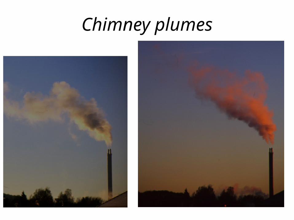
Chimney plumes

One more

• Why do the plumes look different on in different situations?

• Why do they rise to different extents?

• Are there other types of emissions that do not rise to the same extent?

• What does this mean for risks with air pollution?

Inversion

• Temperaturen increases with height

• Reduces air mixing (strongly)

• Ground inversion is most common

• Height inversion – may (more rarely) be important for air pollution levels

• Let us do in on the black/whiteboard …

Unstable

Neutral

Stable

Extremely stable

The gaussian plume model

What is the implication of emission height? Emission temperature? Day/night Summer/winter?

Inversion and traffic sources

In the winter inversions somtimes last over sevelr days? Role of topography?

Now a number of examples of the air pollution situation in Göteborg

January 2005

Nitrogen oxides (NOx = NO + NO2)Femman January 2005

0

200

400

600

800

1000

1200

1400

1600

01/01/2005

03/01/2005

05/01/2005

07/01/2005

09/01/2005

11/01/2005

13/01/2005

15/01/2005

17/01/2005

19/01/2005

21/01/2005

23/01/2005

25/01/2005

27/01/2005

29/01/2005

31/01/2005

Time

NO

x (µ

g/m

3)

NO2 – considered the more toxicFemman January 2005

0

50

100

150

200

250

2005-01-01

2005-01-03

2005-01-05

2005-01-07

2005-01-09

2005-01-11

2005-01-13

2005-01-15

2005-01-17

2005-01-19

2005-01-21

2005-01-23

2005-01-25

2005-01-27

2005-01-29

2005-01-31

Time

NO

2 (µ

g/m

3)

Air q

ualit

y st

anda

rds

Wind speed – very dynamicFemman January 2005

0

2

4

6

8

10

12

14

16

18

01/01/2005

03/01/2005

05/01/2005

07/01/2005

09/01/2005

11/01/2005

13/01/2005

15/01/2005

17/01/2005

19/01/2005

21/01/2005

23/01/2005

25/01/2005

27/01/2005

29/01/2005

31/01/2005

Time

Win

dsp

eed

(m

/s)

Particles – PM10mass of particles < 10 micrometer per cubic metre air

Femman January 2005

0

20

40

60

80

100

120

140

160

01/01/2005 00:00

03/01/2005 00:00

05/01/2005 00:00

07/01/2005 00:00

09/01/2005 00:00

11/01/2005 00:00

13/01/2005 00:00

15/01/2005 00:00

17/01/2005 00:00

19/01/2005 00:00

21/01/2005 00:00

23/01/2005 00:00

25/01/2005 00:00

27/01/2005 00:00

29/01/2005 00:00

31/01/2005 00:00

Time

PM

10 (

µg

/m3)

Relation PM10 with wind speedFemman January 2005

y = 5.1687x - 23.841

R2 = 0.7496

y = -7.6509x + 64.891

R2 = 0.0406

0

20

40

60

80

100

120

140

160

0 2 4 6 8 10 12 14 16 18

Windspeed (m/s)

PM

10 (

ug

/m3)

January

8 January

14 January

Linjär (8 January)

Linjär (14 January)

Femman January 2005

0

0,2

0,4

0,6

0,8

1

1,2

1,4

1,6

1,8

2

2005-01-01

2005-01-03

2005-01-05

2005-01-07

2005-01-09

2005-01-11

2005-01-13

2005-01-15

2005-01-17

2005-01-19

2005-01-21

2005-01-23

2005-01-25

2005-01-27

2005-01-29

2005-01-31

Time

CO

(m

g/m

3)

Carbon monoxide, CO

Chemical and physical conversion

• Oxidation – e.g. of NO2 to HNO3 and of SO2 to H2SO4

• Decomposition (oxidation) of VOC to CO2 and H2O

• Formation of ozone from NO2 and VOC

• Particle formation and growth

Processes in particle formation and conversion

Ozone formation in the troposphere

VOC chemistry

sunlight NO2-NO-O3 cycle

Step by step

Leyton´s formlula The photostationary state

NO

NO

k

JO 2

3

J is the constant of photolysis of NO2:k is the rate constant for the reaction

ONOhNO nmJ 410,2

223 ONOONO k

1 Rodes and Holland

2 Rodes och Holland

3 Rodes och Holland

4 Rodes och Holland

Less ozone injury close to the road

Variation in ozone concentrations

Influence of NO titration on [O3]

00 02 04 06 08 10 12 14 16 18 20 2210

15

20

25

30

35

40

45

Ozo

ne (

nmol

mol

-1)

Time of day

ÖstadRåöFemman

a

00 02 04 06 08 10 12 14 16 18 20 220

5

10

15

20

25

30

35

40

45

Mix

ing

ratio

(nm

ol m

ol -1

)

Time of day

O3

NO

NO2

b

Östad – rural, inlandRåö – rural, coastal

Femman – urban, coastal

Femman - urban

Primary NO2 fraction - increasing

0 100 200 300 400 500 600 700 800 9000.00

0.20

0.40

0.60

0.80

1.00

1.20

Gårda

[NOx], ppb

[NO

2]/[

NO

x], p

pb

Deposition

• Wet deposition – with precipitation

• Dry deposition – as gas or with particles

• For gases – reactivity with surfaces important

• Uptake in organisms – e.g. plant and humans – represent deposition

Effects

• Reduced growth, yield, quality etc of plants

• Health effect – morbidity, mortality

• Effects on materials

• Climate effects

• Effects on the ozone layer in the stratosphere

The urban landscape

• 2

• 3• 4

• 5

• 6 • 7

1 2 3 4 5 6 7 80

20

40

60

80

100

120Passive samplers

Site

Co

nce

ntr

atio

n (

µg

/m3)

NO2NOO3

0

5

10

15

20

25

30

35

1 2 3 4 5 Totalt

Mätperiod

NO

2 (p

pb)

SlottsskogenFemmanFrölundaBjörkekärrOlskroken

NO2 summer 2007

Five periods, one week each

Urban background vs. traffic route

0

20

40

60

80

100

120

140

160

180

06-02-0600:00

06-02-0612:00

06-02-0700:00

06-02-0712:00

06-02-0800:00

06-02-0812:00

06-02-0900:00

tid

[NO

2],

μg

m-3

Femman

Gårda

Example of an urban model

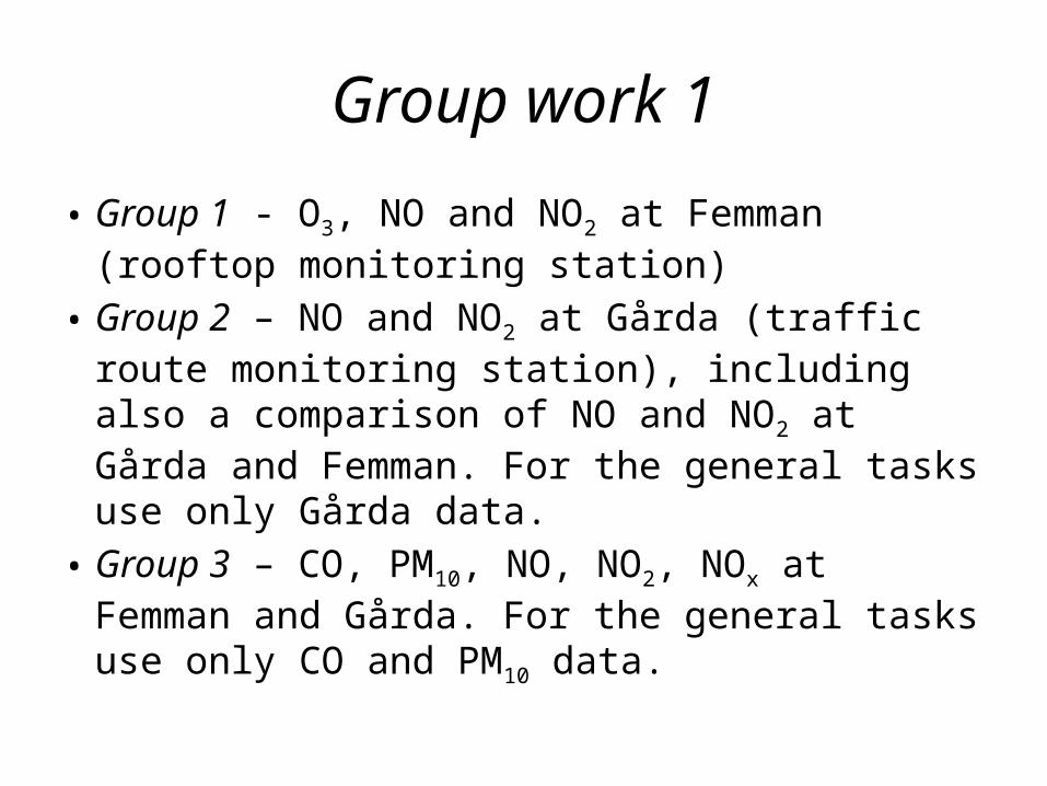
Group work 1

• Group 1 - O3, NO and NO2 at Femman (rooftop monitoring station)

• Group 2 – NO and NO2 at Gårda (traffic route monitoring station), including also a comparison of NO and NO2 at Gårda and Femman. For the general tasks use only Gårda data.

• Group 3 – CO, PM10, NO, NO2, NOx at Femman and Gårda. For the general tasks use only CO and PM10 data.

General tasks

• Plot the average diurnal variation of the pollutants for the whole year! What time of the day do the pollutants typically peak and when is the minimum? What might be the reasons the pollutants peaking at this particular time of the day. Note that the answer may not be one single factor.

• Which season of the year (Spring = March-May, Summer = June-August, Autumn = September-November, Winter = December-February) has the highest and lowest average levels of the different pollutants, respectively. Try this for average values and for the 98-percentile of the different pollutants in the different seasons. Please explain the observed pattern.

Specific tasks Group 1

• Calculate the relationship (photostationary state, explained in lecture) [NO][O3]/[NO2]. How is it related to global radiation (Rad)? You can for example calculate the average of the relationship for the following global radiation intervals: 5-100, 100-200, 200-300, 300-400, 400-500 W m-2. Try to explain the observed pattern.

• Study the limited number of situations (hours) with high ozone concentrations (> 100 µg m-3). What are the characteristics of these situations with respect to season, time of the day and meteorology? Explain your observations.


• Compare the ratio [NO]:[NO2] at Femman and Gårda. In which of the sites is the ratio higher? Why? Also study the [NO]:[NO2] ratio with respect to its relationship with meteorological variables.

• How large is the difference (absolute and relative) in [NOx], [NO] and [NO2] concentration between Femman and Gårda (average and 98-percentile). How are these differences related to weather conditions, especially wind speed and temperature inversion?


• Plot the relationship between the four pollutants and wind speed. Do this for all hourly values and for daily average values. What is the relationship between the concentrations of the different pollutants and wind speed? How much does it differ between different pollutants and why does it differ?

• Calculate [NO2]/[NOx] and plot it vs. [NOx] (molar units, hourly values). What does the plot tell us about the primary NO2 fraction of the vehicle exhausts?

Why percentiles?• The 98-precentile is the concentration which is

exceeded 2% of the time• The 50-percentile is also called the median• To represent the high end of the exposure

without being very sensitive to single values• Very common in setting air quality standards –

AQS• What is the 10-percentile of: 5, 8, 10, 11, 2,

22, 30, 14, 7, 18, 3, 10, 9, 9, 4, 5, 13, 17, 11, 1?

Converion between mass and molar unitsStarting point: the ideal gas law:

eq 1

In this equation p is pressure (unit Pa (Pascal) or N/m2), V is volume (m3), n is amount of substance of gas (moles), R is the universal gas constant (8,31 J mol-1 K-1) and T is the absolute temperature (K).

The amount of substance n can also be expressed as:

eq 2

where m is massa (g) and M is the molar mass (g mol-1). By combining eqs 1 and 2 we get:

eq 3

These principlses apply to each gas (i) in a mixture. Applying this and rearranging eq 3 results in: skrivas som:

eq 4

Why use molar units?

• AQS often use mass units – simple to understand and explain to policy makers etc

• If you wish to compare different gases, sum or subtract them you need to use molar units (e.g. ppb or ppm) – e.g. if you wish to sum NO and NO2 to NOx

• Such as for Leyton´s formula• ppb and ppm is like percent, but where % is pars of

hundred, ppb is part per billion and ppm is parts per million

Data baseFEMMAN GÅRDA LEJONET

Datum timmeCO (µg m-3)

NO (µg m-3)

NO2 (µg m-3)

O3 (µg m-3)

PM10 (µg m-3)

Lufttryck (hPa)

Rel. Fukt (%)

Temp (°C)

V-hast (m s-1)

V-rikt (°) Rad (W m-2)

NO (µg m-3)

NO2 (µg m-3) V-hast (m s-1)Diff T (°C) V-hast (m s.1)

2010-01-01 00:00 0 133 54.0 62.8 8.5 57.6 1001.2 86.5 -7.3 0.8 88 0.0 74.73 108.3 0.7 -0.1 0.52010-01-01 01:00 1 135 18.2 44.7 14.2 62.0 1001.1 87.0 -7.4 1.7 348 0.0 46.37 101.3 1.8 -0.1 1.22010-01-01 02:00 2 144 7.4 29.1 36.0 30.7 1000.9 87.2 -7.4 1.5 336 0.0 35.49 81.3 1.0 -0.1 0.72010-01-01 03:00 3 152 7.4 36.4 32.6 32.6 1000.6 87.6 -6.9 1.2 15 0.0 18.7 61.4 0.9 -0.1 0.82010-01-01 04:00 4 148 6.0 32.2 38.4 21.5 1000.5 89.0 -6.8 1.9 4 0.0 10.9 61.2 1.2 -0.1 1.22010-01-01 05:00 5 150 13.2 35.6 36.2 17.6 1000.6 88.4 -6.9 2.0 8 0.0 23.05 51.9 1.4 -0.1 1.32010-01-01 06:00 6 148 8.9 24.2 40.1 15.0 1000.6 89.5 -6.8 2.0 10 0.0 17.74 46.9 1.2 -0.1 1.52010-01-01 07:00 7 128 10.6 21.8 42.0 10.3 1000.9 89.6 -6.9 3.1 18 0.0 12.78 22.6 1.5 0.0 2.12010-01-01 08:00 8 118 12.0 30.8 37.0 8.2 1001.3 87.5 -6.6 3.3 40 1.0 11 9.7 1.4 0.1 2.32010-01-01 09:00 9 107 13.5 24.6 36.4 7.9 1001.7 87.3 -6.9 3.4 29 19.6 3.08 4.3 1.8 0.0 2.12010-01-01 10:00 10 89 10.8 14.3 37.0 7.1 1002.1 86.5 -6.8 3.8 27 40.0 13.8 9.6 1.7 -0.1 2.32010-01-01 11:00 11 78 20.6 20.9 25.9 7.1 1002.4 84.9 -6.8 2.9 36 47.3 4.51 8.7 1.6 -0.1 2.12010-01-01 12:00 12 64 16.3 15.4 25.7 6.9 1002.5 85.1 -6.6 3.2 32 44.7 14.48 20.2 1.5 -0.1 2.42010-01-01 13:00 13 65 15.2 15.3 26.1 7.5 1002.7 84.2 -6.5 3.5 29 66.6 21.18 23.8 1.8 -0.1 2.32010-01-01 14:00 14 55 16.3 16.5 23.8 7.1 1003.2 83.7 -6.4 3.7 26 33.7 29.6 33.7 1.7 0.0 2.02010-01-01 15:00 15 52 18.8 18.2 21.7 8.3 1003.6 84.6 -6.4 4.0 30 4.9 17.1 30.6 1.9 -0.1 2.52010-01-01 16:00 16 45 19.0 17.5 20.3 7.5 1004.2 85.7 -6.6 4.1 32 0.0 33.65 35.1 2.0 0.0 2.22010-01-01 17:00 17 38 16.0 18.2 20.7 7.5 1004.6 85.1 -6.8 3.6 33 0.0 33.38 37.3 1.6 0.1 2.42010-01-01 18:00 18 110 16.7 19.5 18.4 7.4 1005.1 84.8 -6.7 3.5 33 0.0 20 36.4 1.6 0.1 2.02010-01-01 19:00 19 78 17.1 22.1 20.2 8.2 1005.8 84.9 -6.8 4.0 31 0.0 36.27 40.7 1.7 0.0 2.12010-01-01 20:00 20 85 14.0 17.6 20.1 9.0 1006.4 84.6 -6.6 4.0 32 0.0 18.5 19.3 2.0 0.0 2.22010-01-01 21:00 21 38 13.8 14.7 20.1 10.4 1007.1 86.6 -6.5 4.5 32 0.0 8.63 17.4 1.9 0.0 2.62010-01-01 22:00 22 33 8.9 12.4 23.3 9.5 1007.6 87.7 -6.2 5.2 31 0.0 15.4 13.3 2.4 0.0 3.32010-01-01 23:00 23 71 12.6 12.3 24.0 8.1 1008.1 87.2 -6.0 5.2 33 0.0 6.78 11.9 2.4 0.0 3.4

• Questions: [email protected]

• Supervision of all groups: 18 December 13:00 – 15:00

mailto:[email protected]

Air Pollution and Climate Håkan Pleijel Biological and Environmental Sciences.

Documents

Transcript of Air Pollution and Climate Håkan Pleijel Biological and Environmental Sciences.