Air Pathway Analysis

Mustafa M. Aral

MESL @CEE,GThttp://mesl.ce.gatech.edu/

maral@ce.gatech.edu

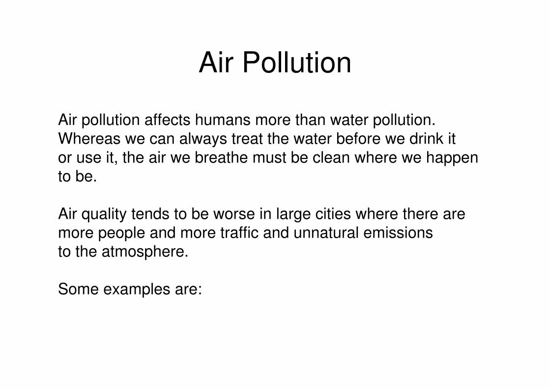
Air Pollution

Air pollution affects humans more than water pollution.

Whereas we can always treat the water before we drink it

or use it, the air we breathe must be clean where we happen to be.

Air quality tends to be worse in large cities where there are

more people and more traffic and unnatural emissions to the atmosphere.

Some examples are:

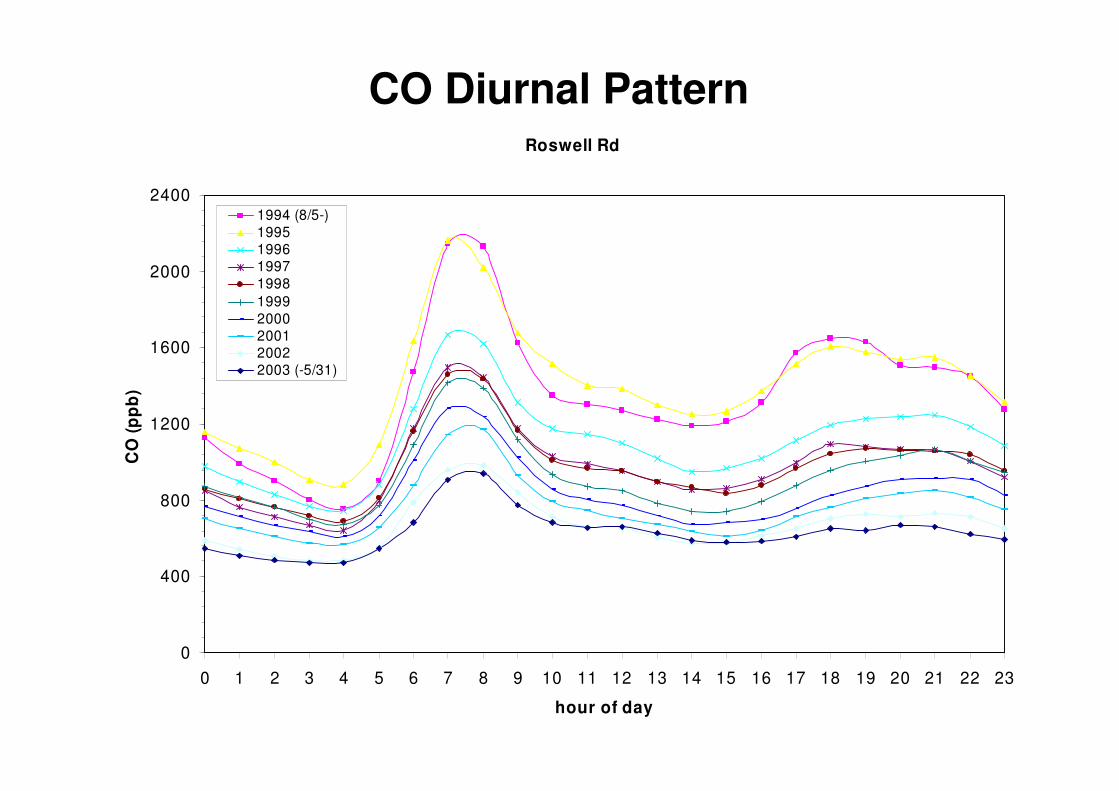
CO Diurnal PatternRoswell Rd

0

400

800

1200

1600

2000

2400

0 1 2 3 4 5 6 7 8 9 10 11 12 13 14 15 16 17 18 19 20 21 22 23

hour of day

CO

(p

pb

)

1994 (8/5-)1995199619971998

19992000200120022003 (-5/31)

SO2 Diurnal Pattern

Georgia Tech

0

2

4

6

8

10

0 1 2 3 4 5 6 7 8 9 10 11 12 13 14 15 16 17 18 19 20 21 22 23

hour of day

SO

2 (

pp

b)

19931994199519961997

19981999200020012002

O3 Diurnal Pattern

Confederate Ave.

0

20

40

60

80

0 1 2 3 4 5 6 7 8 9 10 11 12 13 14 15 16 17 18 19 20 21 22 23

hour of day

O3

(p

pb

)

19931994199519961997

19981999200020012002

Concern: Fine Particulate Matter

Nearly all of southeast is above 15 µg/m3 fine PM

Regulations

CLEAN AIR ACT with amendments:

1955,……, 1963, 1966, 1970 and 1990

NATIONAL AMBIENT AIR QUALITY STANDARDS:

1980 →→ 1988

Ambient Air Pollution

NOx + HC

PM CO + PM

uv

PM SO2

Stationary Sources Mobile Sources

O3

Standards for 6 Chemicals

Pollutant Exposure

Duration

NAAQS Health and Environmental

Outcome

CO 1 hour

8 hours

35 ppm

9 ppm

Headaches, asphyxiation

Angina, pectoris

NO2 1 year 0.053 ppm Respiratory disease

SO2 3 hours

1 day

1 year

0.50 ppm

0.14 ppm

0.03 ppm

Shortness of breath,

Odor, acid precipitation

O3 1 hour

8 hours

0.12 ppm

0.075 ppm

Eye irritation, breathing damage,

bronchitis, heart attack.

Pb 3 months 1.5 µg/m3 Blood poisoning

PM2.5 24 hours

1 year

35 µg/m3

15 µg/m3

Lung damage

PM10 24 hours 150 µg/m3 Respiratory disease, Visibility

Computational Sequence

Source Emissions

Domain Idealization

Atmospheric Conditions

Selection of the Model

Solution and Analysis Uncertainty Analysis

Source EmissionsEmission from water surfacesEmission from Land disposal

Landfills

Source Emissions

Highways

Source Emissions

Stacks

Indoor Air Pollution

Gaussian model

2

2

2

2

x

x

C C Cv R

t x xD

DC C

v Rx x

∂ ∂ ∂+ = +

∂ ∂ ∂

∂ ∂= +

∂ ∂

Key parameter is the Diffusion Coefficient in this calculations

And it depends on the atmospheric stability conditions.

Atmospheric Stability• Thermal stratification is often observed in the atmosphere,

especially over diurnal cycle.

• When it occurs stratification is characterized by colder denser air sinking below lighter and warmer air.

• This stratification creates an obstacle to turbulence and dispersion of contaminants.

• If the air stays stationary in stratified layers instead of mixing vertically, than contaminant concentration will not diminish.

• Thus understanding of stratification and defining a measure of stratification is important.

Atmospheric Stability is Defined in

terms of Lapse Rates• Lapse rate is defined as the manner in which the temperature in an

air packet changes with altitude or elevation.

• A positive lapse rate implies a decrease in temperature with elevation.

• Environmental Lapse Rate(ELR) refers to the variation ofthe temperature with altitude ata certain place and time. (Function of space and time)

Z

T

ELR

θ1

Lapse Rates

• Adiabatic Lapse Rate (ALR) (heat exchange is

not considered).

• Diabatic process in which heat is added or

subtracted from the system, (solar heating,

radiation cooling).

• Dry Adiabatic Lapse Rate (DALR) and the

Saturated Adiabatic lapse Rate (SALR).

Moisture contents controls the heat transfer.

Lapse Rates

• Dry adiabatic lapse rate is the rate at which non-saturated air parcel cools as it rises. This rate is 9.8oC/km or ~ 1oC/100m

• The SALR is variable since it depends on how much the latent heat is made available as the condensation occurs for a saturated air parcel.

Rate Comparisons

Z

TT

Z

ALR > ELR

θ2 > θ1

ALR < ELR

θ1 > θ2

ALR

θ2

ELR

θ1

ELR

θ1

ALR

θ2

∆T ∆T

ALR > ELR ALR < ELR

a. Three mechanical stability conditions [displacement ; tendency]

T

Z P

ALR

ELR

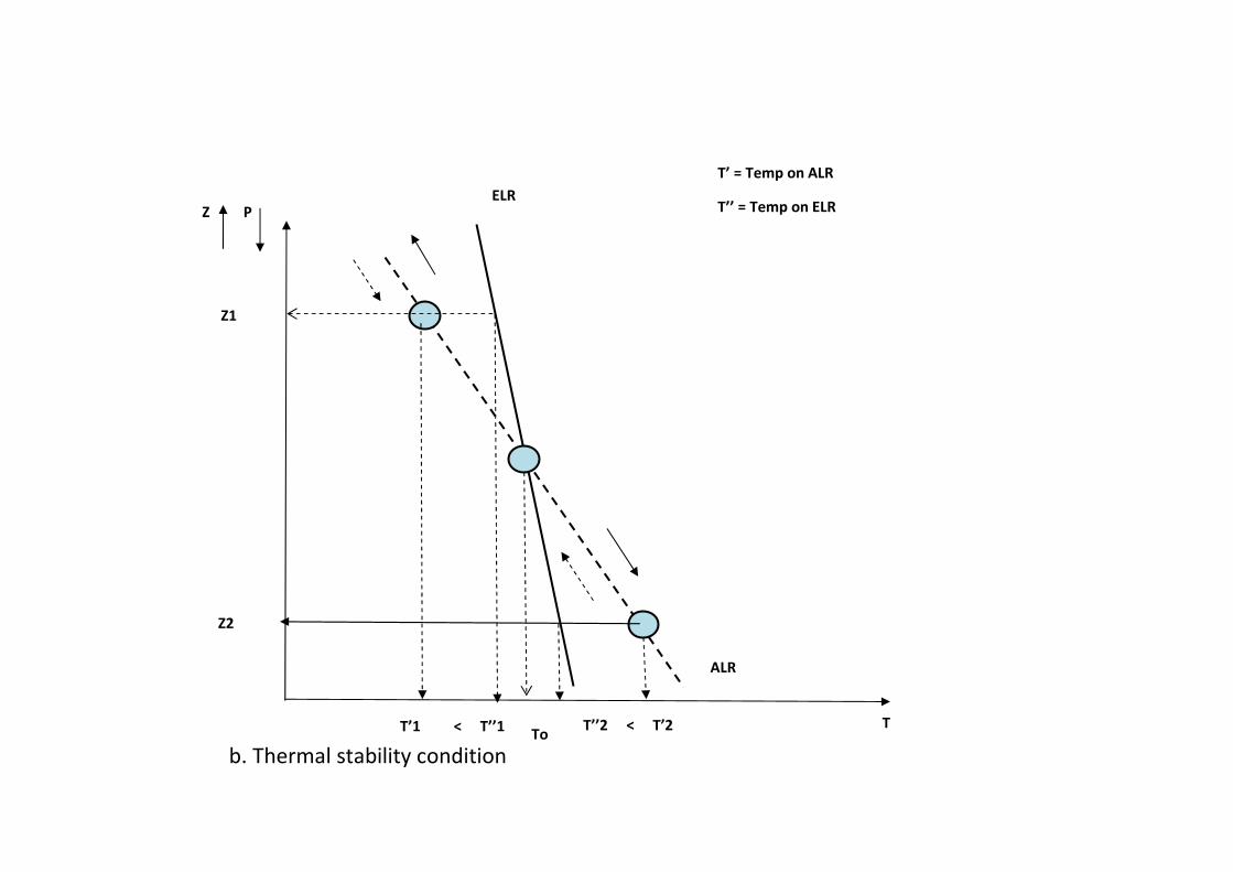
b. Thermal stability condition c. Thermal instability condition

ALR

ELR

Z P

T

NeutralStable Unstable

T

Z P

ALR

ELR

b. Thermal stability condition

Z1

T’1 < T’’1To

Z2

T’’2 < T’2

T’ = Temp on ALR

T’’ = Temp on ELR

T

Z P ALRELR

c. Thermal instability condition

Z1

T’1 > T’’1To

Z2

T’2 < T’’2

T’ = Temp on ALR

T’’ = Temp on ELR

Stability Conditions

• Absolute instability occurs when ELR is greater than DALR. As we know that DALR is 9.8oC/km, than we can conclude that absolute instability exists when ELR is equal or greater than 9.8oC/km. This condition is sometimes identified as “super-adiabatic lapse rate” since the heat loss is very rapid.

• Natural instability occurs when the ELR and DALR are equal. In this term the word “natural” refers to the fact that thermal momentum is not going to be accelerated or decelerated.

• Conditional instability occurs when ELR is less than DALR but more than SALR. SALR is usually considered to be in the range 3.9oC/km - 7.2oC/km. The use of the word “condition” is associated with the condition that instability will only occur when the thermal becomes saturated and before.

• Absolute stability occurs when ELR is less than SALR.

• Potential instability occurs when air at lover elevations is moist but it is dryer at higher elevations. The potential for instability is only realized when the thermal ascends and reaches saturation.

Stability Analysis

W

dx

dz

P1P2

P3

P4

Z

X

Air

Pocket

3 4 0P P W− − =

( ) ( )p z dz p z gdzρ+ − = −

dpg

dzρ γ= − = −

Hydrostatic conditions

unknowns: ; ;dP d dT

dz dz dz

ρ

Pressure vs Elevation:

Equation of state:

• The atmosphere is a mixture of gases (78% Nitrogen, 21% Oxygen, 1% other gases) collectively it as called air.

• Mixture is not so important for this analysis. Let’s consider air to be ideal gas, with a molecular weight between oxygen and nitrogen.

• For an ideal gas Equation of state links pressure, density and temperature as follows:

P R Tρ=T = absolute Temperature degrees Kelvin (= deg Centigrade + 273.15)R=287 J/kg-K 287 m2/s2 -K for air

Equation of state:

P R T

dP d dTR T R

dz dz dz

ρ

ρρ

=

= +

Given the definition of hydrostatic eqn. if a parcel of air rises than its pressure drops.

Given above relation, accordingly its density or temperature or

both should drop as well

But as pressure drops the air parcel expands making its pressure do work against surrounding air parcels.

This work → is associated with internal energy loss = mCvdT

Cv = Heat capacity

Thus internal energy of the parcel drops according to:

vmC dT Pd V= −

2

1v

v

or

C dT Pd

dT P dC

dz dz

ρ

ρ

ρ

= −

=

2

2

1 0

u vu uvd

v v

dd

ρ

ρ ρ

′ ′− =

−=

Pd V

Energy state:

Thus we have three independent equations for three derivatives:

2v

dP

dz

dP d dTR T R

dz dz dz

dT P dC

dz dz

γ

ρρ

ρ

ρ

= −

= +

=

Which can be solved for each derivative

Pressure state

Ideal Gas

Energy state

Solve “say” for temperature gradient:

( )

23

2 2

9.81 /9.76 10 /

1005 /

v

v p

dTC R g

dz

dT g g

dz C R C

dT m sK m

dz m s K

−

+ = −

= − = −+

= − = − ×−

Thus as air pressure decreases as z increases the air

temperature also decreases according to the equation above.

Meteorologists call this ADIABATIC LAPSE.

About 1 deg. drop/100m (that is why it is cold up there)

= Γ

• All this is for natural conditions.

• However, when the air parcel rises and does work to adjust its temperature according to these principles, it finds an another ambient temperature at the new elevation which it needs to adjust as well.

• Ta = ambient temperature is not equal to Tp = natural temperature

• This temperature difference creates buoyancy forces

( ) ( )a p

p

a p

p

gT T T z dz T z dz

C

dT gT T dz

dz C

− = + − +

− +

�

Net upward force

net

net a

F buoyancy force weight

F Vρ

= −

= pg Vρ− ( )a pg Vρ ρ= −

net

a p

g

P PF V

RT RT

= −

( )net p a

a p

g

PF T T V

RT T= −

p a

net p

a

g

T TF V

Tρ

− =

g

Fb

W

Newton’s law

2

2

( )net

p a

p

a

d dzF m

dt

T TV

Tρ

=

−

2

2

( )p

d dzg m V

dtρ= =

2

2

2

2

2

2

( )

( )

( )

p a

a

p a

a a p

d dz

dt

T T d dzg

T dt

T Td dz g dT gg dz

dt T T dz C

− =

− = = +

p a

net p

a

T TF V

Tρ

− =

g

a p

p

dT gT T dz

dz C

− +

�

earlier

earlier

2

2

( )

a p

p

p

p

d dz g dT gdz

dt T dz C

dT gneutural atmosphere

dz C

dT gunstable atmosphere

dz C

dT gstable atmosphere

dz C

= +

= −

< −

> −

Stability conditions:

GRAPHICALLY

T

Z

Z1

Z2

1oC

100m

oC

Unstable

StableInversionΓΓΓΓ

TaTa

Ta

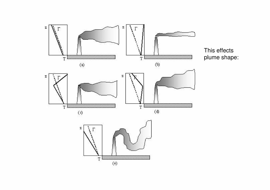
This effects

plume shape:

Gaussian model

2

2

2

2

x

x

C C Cv R

t x xD

DC C

v Rx x

∂ ∂ ∂+ = +

∂ ∂ ∂

∂ ∂= +

∂ ∂

Key parameter is the Diffusion Coefficient in this calculations

And it depends on the stability conditions.

Dispersion coefficients is a function of

Stability Classes

T

Z

A

B

C

D

EF

Inversion

Stable

Unstable

Air Pollution Models

• Atmospheric Stability Analysis– Necessary for Stack height calculations

– Necessary for dispersion constant estimates.

• Air Emission Models– This is mostly for input to air dispersion models except for INDOOR AIR models

– Requires chemical database

– Based on Fickian Diffusion Analysis

– Requires numerous background models

• Air Dispersion Models– Requires chemical database

– Requires Stack height corrections for air dispersion models

– Requires dispersion constants and several other background models

Background correction models are for temperature and density corrections

for different chemicals are based on Henry constant for chemicals in use.

EMISSIONS

Farmer’s Model The Farmer’s model can be used to estimate volatile emissions of a buried

contaminant source below the soil surface.

d1Clean Soil

Contaminated Soil

Emissions V ( ) ( )2

1

10vs a

e

C CE AD

d

−=

E: steady state emission rate of the gases (g/s)

A: surface area of the contamination source (m2)

De: Effective diffusion coefficient of the

contaminant for air (cm2/s)

Cvs: vapor phase concentration of the

contaminant (g/cm3),

Ca: air concentration of the contaminant at soil

surface (g/cm3) (usually assumed to be equal to zero)

d1: the depth of soil cover (m)

And 102 is the conversion factor

Farmer’s ModelThe user should also note that the emission rate output is presented in the units of

(kg/yr) in the output window. The conversion from (g/s) to (kg/yr) is carried out

internally in the ACTS model.

There are several internal computations done in ACTS in this case as will be the

case for all models:

In this model, the soil vapor concentration, Cvs (g/cm3) is given by,

C H Cvs w′=

H’ is the dimensionless Henry’s constant (mg/L)/(mg/L) and is defined as, H

HRT

′ =

H is the Henry’s law constant (atm-m3/mole), R is the universal gas constant

(8.21E-5 atm-m3/K) and T is the absolute temperature (oK).

Farmer’s Model

CT is the contaminant concentration in the soil (g-contaminant/g-wet soil),

θT: soil porosity (dimensionless),

ρb: soil bulk density (g-dry soil/cm3-wet soil),

ρw: density of water (g/cm3), Θw: volumetric water content (dimensionless) and

Kd: soil-water partition coefficient, which is a chemical and soil property

dependent parameter ((g/g)/(g/cm3)),

d oc ocK K f=

The aqueous phase concentration, Cw (g/cm3), is calculated by,

( )( )

T b w w

w

T w w b d

CC

H K

ρ θ ρ

θ θ θ ρ

+=

′− + +

Koc : organic carbon partition coefficient ((g/g)/(g/cm3))

foc : fractional organic carbon content of the soil.

Note that the soil porosity value entered should not be less than the volumetric

water content, .

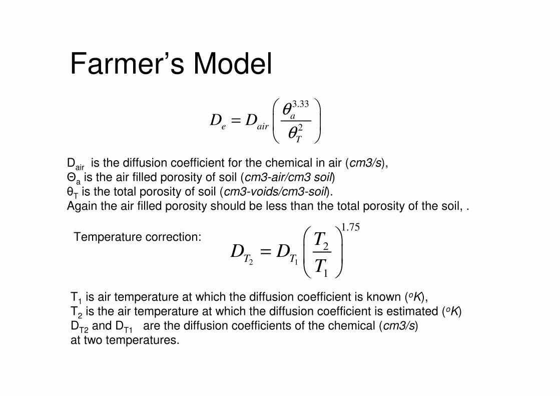
Farmer’s Model3.33

2

ae air

T

D Dθ

θ

=

Dair is the diffusion coefficient for the chemical in air (cm3/s),

Θa is the air filled porosity of soil (cm3-air/cm3 soil)

θT is the total porosity of soil (cm3-voids/cm3-soil).

Again the air filled porosity should be less than the total porosity of the soil, .

2 1

1.75

2

1

T T

TD D

T

=

Temperature correction:

T1 is air temperature at which the diffusion coefficient is known (oK),

T2 is the air temperature at which the diffusion coefficient is estimated (oK)

DT2 and DT1 are the diffusion coefficients of the chemical (cm3/s)

at two temperatures.

Farmer’s Model: Example -1

d1Clean Soil

Contaminated Soil

Emissions

Data:

Clean soil thickness d1 = 400 m

Contaminated soil area A = 200 m2

Background air concentration C = 0 g/m3

Total Soil Contamination Cs = 100 mg/kg

Soil Density = 1.9 g/cm3

Soil porosity n = 0.4 cm3/cm3

Moisture content = 0.15 cm3/cm3

Soil carbon content % = 0.1

Air Temperature = 298 oK

Air Diffusion coeff. = ???

Farmer’s Model

Farmer’s Model MC

Farmer’s Model MC

Farmer’s Model MC

Farmer’s Model MC

Farmer’s Model MC

Linking Farmer’s Model to Box ModelThe Farmer’s model can be used to estimate volatile emissions of a buried

contaminant source below the soil surface.

d1Clean Soil

Contaminated Soil

Emissions V ( ) ( )2

1

10vs a

e

C CE AD

d

−=

E: steady state emission rate of the gases (g/s)

A: surface area of the contamination source (m2)

De: Effective diffusion coefficient of the

contaminant for air (cm2/s)

Cvs: vapor phase concentration of the

contaminant (g/cm3),

Ca: air concentration of the contaminant at soil

surface (g/cm3) (usually assumed to be equal to zero)

D1: the depth of soil cover (m)

And 102 is the conversion factor

Linking Farmer’s Model to Box Model

Linking Farmer’s Model to Box Model

Linking Farmer’s Model to Box Model

Linking Farmer’s Model to Box Model

Farmer’s Model: Assumptions

1. In Farmer’s model it is assumed that the source concentration of contaminants

does not decrease as the emissions occur.

2. Also decay of the contaminant source is not considered.

This implies that the amount of contaminant mass in the soil is infinite;

3. The location of the contaminant source is fixed at a depth below the surface

of the soil;

4. Emissions from the soil originating from the contaminant source are in steady state;

5. The concentration of the chemical in air at the soil surface is negligible as compared

to the vapor concentration within the soil.

Thibadeaux-Hwang Model

d1Clean Soil

Contaminated Soil

Emissions

d2

V

( )2 2 11

2 ( )

e vs

e vs

o

D CE t

D At d d Cd

m

=−

+

2 1( )o b

m d d AC= −

( )b T b w w

C C ρ ρ θ= +

0

1'( ) ( )

t

E t E t dtt

∆

∆ =∆ ∫

Thibadeaux-Hwang Model

ERROR: stackunderflow

OFFENDING COMMAND: ~

STACK: