AIR FORCE INSTITUTE OF TECHNOLOGY · an analysis of construction cost and schedule performance...

AN ANALYSIS OF CONSTRUCTION COST AND SCHEDULE

PERFORMANCE

THESIS

Michael J. Beach, Major, USAF

AFIT/GEM/ENV/08-M02

DEPARTMENT OF THE AIR FORCE AIR UNIVERSITY

AIR FORCE INSTITUTE OF TECHNOLOGY

Wright-Patterson Air Force Base, Ohio

APPROVED FOR PUBLIC RELEASE; DISTRIBUTION UNLIMITED

The views expressed in this thesis are those of the author and do not reflect the official

policy or position of the United States Air Force, Department of Defense, or the U.S.

Government.

AFIT/GEM/ENV/08-M02


PERFORMANCE

THESIS

Presented to the Faculty

Department of Engineering Management

Graduate School of Engineering and Management

Air Force Institute of Technology

Air University

Air Education and Training Command

In Partial Fulfillment of the Requirements for the

Degree of Master of Science in Engineering Management

Michael J. Beach, BS

Major, USAF

March 2008

APPROVED FOR PUBLIC RELEASE; DISTRIBUTION UNLIMITED

AFIT/GEM/ENV/08-M02


PERFORMANCE

Michael J. Beach, BS

Major, USAF

Approved: ________--signed--____________________ 18 Mar 08 Sonia E. Leach, Maj, USAF (Chairman) Date ________--signed--____________________ _18 Mar 08 Alfred E. Thal, Jr., Ph D (Member) Date

AFIT/GEM/ENV/08-M02

Abstract

Cost and schedule performance are widely accepted in the literature and in industry as

effective measures of the success of the project management effort. Earned Value

Analysis (EVA) is one method to objectively measure project cost and schedule. This

research evaluates the cost and schedule performance of 1,322 completed United States

Air Force (AF) Military Construction (MILCON) projects, executed from 1990 to 2005.

The impact of Major Command (MAJCOM), Construction Agent (CA), facility type

(CATCODE), individually and in combination, on the EVA metrics of Cost Performance

Index (CPI), Time Performance Index (TPI), and CPI*TPI were evaluated. The results

indicate that AF MILCON projects are typically executed either on or below their

respective budgets, but typically take more time than expected for construction. This

outcome implies that AF MILCON projects trade time performance in an effort to control

costs. When cost and performance are given equal weight, the sacrifice made in time

performance is greater than the benefit gained in cost performance.

v

Table of Contents

Page

Abstract .............................................................................................................................. iv

Table of Contents.................................................................................................................v

List of Figures .................................................................................................................. viii

List of Tables ..................................................................................................................... ix

AN ANALYSIS OF CONSTRUCTION COST AND SCHEDULE PERFORMANCE....1

I – Introduction ....................................................................................................................1

Planning and Programming ..........................................................................................1

Design and Construction ..............................................................................................2

MILCON Execution Agencies. ....................................................................................3

Motivation ....................................................................................................................4

Problem Statement........................................................................................................5

Research Questions ......................................................................................................5

Data and Analysis Methodology ..................................................................................6

Thesis Overview...........................................................................................................8

II. Literature Review............................................................................................................9

Development of the Project Management Discipline...................................................9

Facility Project Critical Success Factor Development ...............................................11

Evolution of Facility Project Success Criteria............................................................14

III. Methodology................................................................................................................19

Introduction ................................................................................................................19

Source Data ................................................................................................................19

Analysis Metrics.........................................................................................................21

vi

Page

Hypotheses, and Analysis of Variance (ANOVA) tests.............................................23

Interpretation of Results .............................................................................................26

IV. Analysis and Results....................................................................................................27

Distribution of Analysis Metrics ................................................................................27

Research Question 1 ...................................................................................................29

MAJCOM CPI Performance ......................................................................................30

MAJCOM TPI Performance.......................................................................................33

MAJCOM CPI*TPI Performance ..............................................................................35

Research Question 2 – ................................................................................................37

MAJCOM-CA CPI Performance ...............................................................................37

MAJCOM-CA TPI Performance................................................................................40

MAJCOM-CA CPI*TPI Performance .......................................................................43

CA CPI Performance..................................................................................................47

CA TPI Performance ..................................................................................................49

CA CPI*TPI Performance..........................................................................................51

Research Question 3 ...................................................................................................55

CATCODE CPI Performance.....................................................................................56

CATCODE TPI Performance.....................................................................................58

CATCODE CPI*TPI Performance.............................................................................60

MAJCOM-CATCODE CPI Performance ..................................................................62

MAJCOM-CATCODE TPI Performance ..................................................................64

vii

Page

MAJCOM-CATCODE CPI*TPI Performance ..........................................................65

CA-CATCODE CPI Performance..............................................................................67

CA-CATCODE TPI Performance..............................................................................69

CA-CATCODE CPI*TPI Performance......................................................................72

MAJCOM-CA-CATCODE CPI Performance ...........................................................74

MAJCOM-CA-CATCODE TPI Performance ...........................................................76

MAJCOM-CA-CATCODE CPI*TPI Performance ...................................................78

V. Conclusions and Recommendations ............................................................................81

Conclusions ................................................................................................................81

Limitations..................................................................................................................85

Contributions ..............................................................................................................86

Opportunities for Future Research .............................................................................87

Bibliography ......................................................................................................................88

viii

List of Figures

Page

Figure 1 Research Flow Chart ............................................................................................ 7

Figure 2 EVA Metric Notional Data................................................................................. 23

Figure 3 AF CPI, TPI, and CPI*TPI Distribution, N=1322 ............................................. 29

ix

List of Tables

Page

Table 1 DoD MILCON and Total Budget and its Percentage in FYs 2004-7.....................4

Table 2 Description of Data Fields Utilized in this Research............................................20

Table 3 Explanation of EVA Variables and Metrics .........................................................21

Table 4 ANOVA Hypothesis Tests for Performance Metrics ...........................................24

Table 5 Categories, Minimum Sample Size, and Number of Items in Each Category......28

Table 6 MAJCOM Names and CPI Descriptive Statistics N = 1266 ................................31

Table 7 MAJCOM CPI One-Way ANOVA Results .........................................................33

Table 8 MAJCOM TPI Descriptive Statistics N = 1266 ...................................................34

Table 9 MAJCOM TPI One-Way ANOVA Results..........................................................35

Table 10 MAJCOM CPI*TPI ANOVA Descriptive Statistics..........................................36

Table 11 MAJCOM CPI*TPI One-Way ANOVA Results ...............................................37

Table 12 MAJCOM-CA Names and CPI Descriptive Statistics .......................................39

Table 13 MAJCOM-CA CPI One-Way ANOVA Results ................................................40

Table 14 MAJCOM-CA TPI Descriptive Statistics N = 514 ............................................41

Table 15 MAJCOM-CA TPI One-Way ANOVA Results.................................................42

Table 16 MAJCOM-CA CPI*TPI ANOVA Descriptive Statistics N = 514.....................44

Table 17 MAJCOM CPI*TPI One-Way ANOVA Results ...............................................45

Table 18 CA Names and CPI Descriptive Statistics N = 1,004.........................................48

Table 19 CA CPI One-Way ANOVA Results...................................................................49

Table 20 CA TPI Descriptive Statistics .............................................................................50

x

Page

Table 21 CA TPI One-way ANOVA Results ....................................................................51

Table 22 CA CPI*TPI ANOVA Descriptive Statistics .....................................................52

Table 23 CA CPI*TPI One-Way ANOVA Results...........................................................53

Table 24 CATCODE with names and CPI Descriptive Statistics N = 1,095 ....................56

Table 25 CATCODE CPI One-Way ANOVA Results......................................................58

Table 26 CATCODE TPI Descriptive Statistics N = 1095 ...............................................59

Table 27 CATCODE TPI One-Way ANOVA Results......................................................60

Table 28 CATCODE CPI*TPI ANOVA Descriptive Statistics N – 514 ..........................61

Table 29 CATCODE CPI*TPI One-Way ANOVA Results..............................................62

Table 30 MAJCOM-CATCODE CPI Descriptive Statistics N = 290...............................63

Table 31 MAJCOM-CATCODE CPI One-Way ANOVA Results ...................................63

Table 32 MAJCOM-CATCODE TPI Descriptive Statistics N = 290 ...............................64

Table 33 MAJCOM-CATCODE TPI One-Way ANOVA Results ...................................65

Table 34 MAJCOM-CATCODE CPI*TPI Descriptive Statistics N = 290.......................66

Table 35 MAJCOM-CATCODE CPI*TPI One-Way ANOVA Results ...........................66

Table 36 CA-CATCODE and CPI Descriptive Statistics N = 408....................................68

Table 37 CA-CATCODE CPI One-Way ANOVA Results...............................................69

Table 38 CA-CATCODE TPI Descriptive Statistics N = 408...........................................70

Table 39 CA-CATCODE TPI One-Way ANOVA Results...............................................71

Table 40 CA-CATCODE CPI*TPI Descriptive Statistics N = 408 ..................................73

Table 41 CA-CATCODE CPI*TPI One-Way ANOVA Results.......................................74

xi

Page

Table 42 MAJCOM-CA-CATCODE CPI Descriptive Statistics N = 131........................75

Table 43 MAJCOM-CA-CATCODE CPI One-Way ANOVA Results ............................76

Table 44 MAJCOM-CA-CATCODE TPI Descriptive Statistics N = 131 ........................77

Table 45 MAJCOM-CA-CATCODE TPI One-Way ANOVA Results ............................78

Table 46 MAJCOM-CA-CATCODE CPI*TPI Descriptive Statistics N = 131................79

Table 47 MAJCOM-CA-CATCODE CPI*TPI One-Way ANOVA Results ....................80

Table 48 Summary of SSH and SSL performers ...............................................................83

Table 49 Summary of SSH and SSL performers ...............................................................85

1


PERFORMANCE

I – Introduction

The management of project cost, schedule, and quality has a long history in the

construction industry. These three project parameters are frequently at odds with one

another; project managers must actively manage tradeoffs among them until the project is

complete. Air Force Instruction (AFI) 32-1021 defines MILCON as “any construction,

development, conversion, or extension of any kind carried out with respect to a military

installation. MILCON includes construction projects for all types of buildings, roads,

airfield pavements, and utility systems costing $750,000 or more,” (Department of the

Air Force, 2003; p.21) though prior to 2003, projects costing more than $500,000 were

considered as MILCON projects. Funds for MILCON projects are approved bi-annually

by Congress through the Military Construction Appropriations Act, and approved

MILCON projects have five years to be completed before the appropriation expires

(Department of the Air Force, 2003). Given this, the total time needed for a MILCON

project to go from planning to a completed facility usually ranges from three to five years

(Department of the Air Force, 2000). The MILCON cycle consists of four elements:

planning, programming, design, and construction.

Planning and Programming

The planning and programming phases of the MILCON project lifecycle take

place at the base or wing level. The planning and programming processes identify

2

estimated costs and scope of the project, typically including the mission impact of the

new facility, the proposed project location, required utility runs, and any information

regarding environmental impacts associated with the new facility. Installations “identify,

develop, and validate MILCON projects.” Major commands (MAJCOMs) “compile,

validate, and submit” their AF MILCON programs to headquarters (HQ) AF (AFI 32-

1021, 21). The output of the MILCON planning and programming process is the

Department of Defense form 1391 (DD 1391) Military Construction Project Data. “The

DD 1391, by itself, shall explain and justify the project to all levels of the AF, Office of

the Secretary of Defense, Office of Management and Budget, and Congress.”

(Department of the Air Force, 2003: 21) Once the program is approved by the AF

corporate structure, it is submitted to congress, and then signed into law in the president’s

budget; the programmed amounts (PAs) in the law become the projects’ budgets

(Department of the Air Force, 2003: 24).

Design and Construction

Projects that have been approved by congress and the president are able to move

into the design and construction phases. While installations have a large role to play in

the planning and programming of AF MILCON projects, the MAJCOMs retain budget

and scope control in the design and construction phases. For the period included in this

study, execution of approved AF MILCON projects has been delegated to the MAJCOM

level. During the design phase, the basic requirements identified by the planning and

programming process are developed into an actual facility design suitable for

construction contractors to bid on. The design process is when the primary stakeholders

3

in the project are identified and their requirements are documented in the project’s

drawings and specifications. Typically, the stakeholders include the MAJCOM project

manager, the Construction Agent (CA) project manager, and representatives from the

using organization and local civil engineer unit, as a minimum.

The construction phase of the AF MILCON process is when the actual facility

gets built. The construction phase begins when the bidding documents are advertised and

ends when all construction work is complete and has been accepted by the government.

It is common for the government to accept beneficial occupancy when the facility is

substantially complete. The contractor will typically have a punch list of small items

remaining to be corrected before the contract is considered complete, but the facility is

complete enough for the using agency to occupy and operate the facility.

MILCON Execution Agencies.

The MAJCOMs each have their own branches responsible for the design and

construction of their AF MILCON projects. The MAJCOM MILCON management

offices can choose between three agencies to execute their programs: the US Army Corps

of Engineers (USACE), the US Naval Facilities Engineering Command (NAVFAC), and

the Air Force Center for Engineering and the Environment (AFCEE). USACE,

NAVFAC, and AFCEE are referred to as design and construction agents (CA) (AFI 32-

1023, Ch 5-6). The size of the program that can be executed by AFCEE is limited by the

AF MILCON Program Management Plan to five percent of the amount executed by

USACE.

4

Motivation

Today’s AF budget resources are being stretched ever thinner in support of the

global war on terrorism and fleet modernization requirements (Moseley, 2006).

Increasing construction budgets and aging infrastructure means that the AF must apply its

limited capital investment dollars in the most effective manner possible to ensure

adequate support of the mission (America’s aging infrastructure, 2007). Table 1, DoD

MILCON Budget and its Percentage of the Total Budget for FYs 2004-2007, shows how

the MILCON budget as a percentage of the total defense budget has been increasing over

the last four years (Department of Defense, 2007). To ensure optimum mission support,

the efficacy of the AF MILCON program needs to be optimized to the maximum extent

possible.

Table 1 – DoD MILCON and Total Budget and its Percentage FYs 2004-2007

FY MILCON Total MILCON percentage

2004

2005

2006

2007

$6,137

$7,260

$8,938

$12,614

$490,621

$505,796

$491,815

$463,205

1.25 %

1.44 %

1.8 %

2.7 %

Note. Housing MILCON not included

All dollar amounts in millions

5

Problem Statement

The AF needs to allocate scarce MILCON resources for maximum positive

impact on the mission. This research intends to determine if there is statistically

significant variation in the cost and schedule performance of projects based on

MAJCOM, CA, facility type, or any combination of these three factors. This research

investigated if any MAJCOM or MAJCOMs achieve higher levels of cost and schedule

performance than any other MAJCOMs, as well as if there are certain MAJCOM and CA

combinations that achieve higher levels of cost and schedule performance than other

combinations. In addition, this research investigated if there are variations in MAJCOM

or CA performance with respect to the constructed facility type. These differences,

should they exist, will be used to inform AF leaders about the cost and schedule

performance of the agencies associated with AF MILCON project delivery. This

information can then be shared with all AF MILCON project managers to ensure the

program delivers the maximum possible benefit to the AF.

Research Questions

1. Is there a statistically significant difference in the ability of MAJCOMs to

successfully accomplish projects with respect to cost and schedule performance

measures as compared to the other MAJCOMs?

2. Is there a statistically significant difference in the ability of CAs to successfully

accomplish projects for each MAJCOM with respect to cost and schedule

performance measures as compared to other MAJCOM and CA combinations?

6

3. Is there a statistically significant difference in the ability of construction agents to

successfully accomplish projects for each MAJCOM with respect to cost and

schedule performance measures for different types of facilities as compared to

other types of facilities?

4. Can the differences in success between construction agents as determined through

research questions one, two and three, if any, be attributed to pre-project planning

processes?

Data and Analysis Methodology

Analysis will be performed on projects with the following selection criteria:

1. All project locations across the AF.

2. Minimum project value at the MILCON spending level. This level was $500,000

for FY95 to FY02 and $750,000 for FY03 to FY06.

3. All projects will be more than 95% complete between FY90 and FY05.

4. Due to differences in funding and contracting policies, no military family housing

projects or Non-Appropriated Funds (NAF) will be included in this study.

7

Analysis of project success criteria withrespect to MAJCOM, CA, CATCODE,

and combinations of these

Apply SuccessCriteria

Project Data

Compileresults

Compare with expectations

Figure 1 Research Flow Chart

The methodology flow chart in Figure 1 was used to conduct the research process.

The data for this effort was collected from the AF Automated Civil Engineer System –

Project Management (ACES-PM) information system. ACES-PM is the system of record

for all Air Force construction projects. The report from ACES-PM contains data from

1,659 AF MILCON projects from 1990 to 2005 that are at least 95 percent complete.

The ACES-PM data was analyzed using Analysis of Variance (ANOVA) techniques to

objectively measure the differences between each CA’s ability to complete projects that

address the cost and schedule performance measures.

8

Thesis Overview

The remainder of this thesis is organized into four chapters. Chapter Two will

present a review of the previous research conducted in the areas of project success

factors, project success criteria, and the impact of pre-project planning on project success.

Chapter Three will present the data analysis and exploratory research methodology.

Chapter Four presents the results of the data analysis, and Chapter Five presents the

conclusions limitations and contributions of the research, and areas for future research.

9

II. Literature Review

The project management literature has developed critical success factors (CSFs)

and criteria for measuring project success. However, the literature shows limited

consensus regarding a comprehensive list of CSFs. Although, there is also a lack of

consensus regarding an all-encompassing suite of success criteria that delivers consistent

results for all project stakeholders, there is a growing consensus regarding particular

CSFs and success criteria that are applicable to all facility construction projects.

Therefore, this chapter covers the development of the project management field and the

techniques used by academics and practitioners in this field to complete projects

successfully. The emerging CSFs and success criteria with the most concurrence in the

literature will be used in this research in Chapters 3 and 4 to analyze Air Force Military

Construction (AF MILCON) program project data.

Development of the Project Management Discipline

Network Techniques were first applied to project management in the 1950s and

1960s. Network techniques are characterized by separating a project into a series of

inter-connected subtasks known as the work breakdown structure (WBS). The tasks

within the WBS have cost and time allocated to their accomplishment. Two models are

widely used to analyze and monitor the accomplishment of tasks within the WBS: the

program evaluation and review technique (PERT) and critical path method (CPM). The

PERT was developed by the United States (US) Navy in cooperation with Booz-Allen

Hamilton and the Lockheed Corporation to manage the Polaris submarine and missile

program in 1958. Dupont developed the CPM during the same period. The PERT has

10

wide application in research and development projects, while the CPM has garnered

acceptance in the construction industry. The two methods are quite similar; the academic

community frequently combines them for educational presentation. While the PERT was

strictly focused on managing project timelines using probabilistic techniques, the CPM

used deterministic time estimates. CPM was designed to help manage time and cost

trade-offs. Network techniques like the PERT and CPM allow managers to discern a

critical path whose activities cannot be delayed without adversely affecting the project’s

timeline. The PERT and the CPM also identify activities that can be delayed for a certain

amount of time without delaying the project as a whole; these items are said to have slack

or float (Meredith and Mantel, 2000, 307). By monitoring the critical path throughout the

project, managers can apply resources where they will provide the greatest benefit to the

overall project.

The application of PERT and CPM reinforced the importance of schedule and

cost performance in project management; managers were trained to focus on how to

improve project cost, schedule, and quality performance (Dvir & Lechler, 2003:1).

Additionally, the use of earned value analysis or management (EVA or EVM,

respectively) supports project manager’s ability to control project cost and schedule.

EVA facilitates cost and schedule control because its performance indices are calculated

from cost and schedule variances; these are used to forecast project cost and schedule

performance at completion. Because EVA gives indications early in the project’s life-

cycle about the cost and schedule performance of the project at completion, managers can

take corrective actions to ensure timely, on-budget delivery (Anbari, 2003,12). Cost, -

11

schedule, and quality performance have come to be known as the “iron triangle” of

project management (Jha and Iyer, 2007)

Facility Project Critical Success Factor Development

In 1982, Rockart introduced the concept of critical success factors (CSFs) and defined

them as “those few key areas of activity in which favorable results are absolutely

necessary for a particular manager to reach his or her goals.” Although Rockart’s CSFs

were originally introduced in the context of information systems, they have since been

applied to projects in other disciplines.

Ashley, Lurie, and Jaselskis (1987) found that projects benefited from emphasis

in “planning effort (construction and design), project manager goal commitment, project

team motivation, project manager technical capabilities, scope and work definition, and

control systems.” Their study focused on the difference between average and outstanding

projects; it generated an initial list of approximately 2,000 factors. The list was derived

from literature review and construction project personnel interviews. Similar factors

were then combined, resulting in 46 factors that were subjectively grouped into five

major categories: 1) management, organization and communication, 2) scope and

planning, 3) controls, 4) environmental, economic, political, and social, and 5) technical.

Input from several construction project personnel representing both owners and

contractors was obtained; 11 of the 46 factors from the list of 2,000 were selected for

further analysis. A survey and structured interview of construction personnel from eight

companies was then conducted. The purpose of the second survey and construction

12

interview was to determine if the factors derived from the first set of interviews could be

statistically correlated to project success.

The results of the objective and subjective data from the study were statistically

analyzed using several different techniques. Two-sample hypothesis tests were

accomplished to determine whether the differences in average percentages found were

statistically significant. Correlation analysis was then done to determine if the factors

had a causal effect on construction project success. The analysis found 6 of the 11

factors, planning effort (construction and design), project manager goal commitment,

project team motivation, Project Manager (PM) technical capabilities, scope and work

definition, and control systems achieved statistically significant differences between the

mean values of the average and outstanding projects (Ashley, Lurie, and Jaselskis,

1987:72).

Sanvido, Grobler, Parfitt, Guvenis, and Coyle (1992) were the first to apply

Rockart’s (1982) CSFs specifically to construction. Even though their investigation

uncovered many definitions of success, common success criteria began to emerge.

Designers, owners, and contractors all recognized the financial needs of the other parties;

owners need projects completed on time and on budget while designers and contractors

need profits. Additionally, all three parties agree that projects free from litigation are

more likely to be considered successful (Sanvido et al., 1992:96-97). After analysis of 16

projects, Sanvido et al (1992) recommended four CSFs for construction projects in order

of priority: the facility team; contracts, changes, and obligations; facility experience; and

optimization information. Interestingly, poor quality design documents were found in

13

both successful and unsuccessful projects, but projects with functional facility teams were

able to work around this deficiency (Sanvido et al., 1992: 110).

According to Gibson and Hamilton (1994:10) pre-project planning for a capital

facility is defined “as the process of developing sufficient strategic information for

owners to address risk and decide to commit resources to maximize the chance for a

successful project”. Since Rockart’s (1982) CSFs were applied to project management

many researchers have found CSFs that are related to the pre-project planning stages.

Gibson and Hamilton (1994) divided pre-project planning into four subprocesses:

organize for pre-project planning; select alternatives; develop project definition package;

and make decision. Gibson and Hamilton (1994) found a “positive, quantifiable,

relationship” (p. x) between effort expended during the pre-project planning phase and

the ultimate success of the project. The effort expended during pre-planning “directly

affects the cost and schedule predictability of the project” (p. x). Survey and interview

instruments were used extensively by Gibson and Hamilton (1994) to determine the

impact of pre-project planning on project success.

In 1999, Chua, Kog, and Loh’s article “Critical Success Factors for Different

Project Objectives” investigated whether the CSFs related to achieving cost, schedule, or

quality performance objectives were independent; for example, are the CSFs related to

cost performance the same as the CSFs for schedule performance? The study found that

each project objective produced a different set of CSFs; however, adequacy of plans and

specifications and constructability emerged as the two most CSFs for all three project

14

objectives. PM competency and PM commitment and involvement were also common to

all three objectives at differing levels of significance (Chua, Kog, and Loh, 1999: 147).

Evolution of Facility Project Success Criteria

Concurrent with the development of CSFs through the 1980s, researchers were

also investigating project success criteria. Researchers began to recognize that

construction projects have many stakeholders with different objectives depending on the

phase of the project (de Wit, 1986: 13).

Even as project management was emerging as a formal discipline in the 1950s

managers recognized that project success primarily involves meeting cost, schedule, and

budget goals (Dvir and Lechler, 2003:1, Freeman and Beale, 1988:68). Gaddis (1954)

discussed the importance of the project manager’s skill to balance emphasis between

performance, budget, and time requirements and the constant conflict between them.

Baker, Murphy, and Fisher (1980) conducted a study of 650 completed National

Aeronautics and Space Administration projects and found that cost and schedule

performance were correlated with project success, but were not found to be linearly

related to perceived success or failure. Additionally, cost and schedule performance were

not part of 29 perceived management characteristics significantly related to perceived

project success or failure. The latter result was attributed to the fact that the projects

studied were already completed, and that the importance of cost and schedule

performance can diminish as time passes and managers forget how critical the budget and

timeline were during a project’s execution phase. By the mid-1980s, researchers began

15

to differentiate between the success of the project itself and the success of the project

management effort. Success criteria that focus solely on cost, schedule, and quality

primarily measure the efficacy of the project management effort (de Wit, 1986: 13).

Pinto and Slevin (1988) found that the concept of project success was

ambiguously understood by project managers and loosely defined in the literature.

Additionally, some projects can initially be perceived as failures but then be viewed as

major successes as time passes, or vice versa (Pinto and Slevin, 1988: 67). One study

found that the most frequently used success criteria in the literature were budget

performance, schedule performance, client satisfaction, and project manager/team

satisfaction (Ashley, Lurie, and Jaselskis, 1988: 69). Pinto and Slevin (1988) introduced

the project implementation success criteria of technical validity, organizational validity,

and organizational effectiveness. A project is technically valid if it works as intended. A

project is organizationally valid if it is “right” for the client and contributes to improved

organizational effectiveness. Lastly, organizational effectiveness “is concerned with

determining whether…it is contributing to an improved level of organizational

effectiveness in the client’s organization” (Pinto and Slevin, 1988: 68-69). Pinto and

Slevin (1988) hypothesized that cost and schedule performance were important success

criteria, but not the only success criteria.

A seemingly straightforward way to measure the success of a project is to

compare the results of the project to the objectives laid out for the project before it was

undertaken. However, problems arise when some objectives are in conflict with others;

this becomes readily apparent when the objectives of different stakeholders are

16

considered. Objectives can change with each major phase of the project over its life-

cycle; this further complicates the measurement of project success. Lastly, there is a

hierarchical dimension to project success as each level of management of an organization

can have different, sometimes conflicting, objectives (de Wit, 1986: 13).

In 1992 Freeman and Beale introduced a technique to objectively measure the

criteria of scope, quality, cost, and duration using discounted cash flow methods like Net

Present Value (NPV). DCF-based project success criteria utilize concepts from

engineering economics to determine if a project was a success. Freeman and Beale

(1992) hypothesized that from the viewpoint of any stakeholder, if the PV of the revenues

is greater than the PV of the costs, then the project can be considered successful. This

study analyzed the DCFs associated with a commercial high-rise building in Sydney,

Australia. The DCFs were analyzed from several points of view to determine if there are

success criteria common to both points of view. The conclusion was that “scope, quality,

cost, and duration” (p 16) could be utilized in a DCF paradigm to develop project success

measures.

Griffith, Gibson, Hamilton, Tortora, and Wilson (1999 categorized projects by

their cost, schedule, and quality performance. Objective values for project quality were

calculated by comparing the project’s design capacity with its actual output. The project

success index is calculated from a formula that assigns values to budget achievement,

schedule performance, percent capacity attained six months after completion, and plant

utilization attained six months after completion. A limitation of the Griffith et al. (1999)

study is that the project must produce measurable outputs; therefore, it is limited to

17

facilities with quantifiable outputs, such as factories, refineries, power plants, and

communications facilities. Projects whose outputs are not directly quantifiable are not

well suited to the project success index. For instance, the increase in an organization’s

effectiveness after the construction of a new corporate headquarters would be very

difficult to objectively measure.

Chan, Scott, and Lam (2002) analyzed 20 studies published from 1990 through

2000 and found that 13 different success criteria were advocated by these studies.

However, 18 of the 20 studies used time, cost, and quality as components of success.

Furthermore, three studies published in the late 1990s used the iron triangle as the sole

means of measuring success (Chan, Scott, Lam, 2002:122).

By the year 2000, researchers were beginning to include subjective measurements

of project success criteria in addition to the well-established objective criteria. Items

such as project management team teamwork in addition to the traditional iron triangle

criteria were evaluated using survey and interview techniques to capture the viewpoints

of different project stakeholders (Hughes, Tippett, and Thomas, 2004).

Anbari (2003) introduced simplified and extended EVA metrics to facilitate

implementing EVA on real-world projects. EVA supports the simultaneous management

of “project scope, time, and cost” (Anbari, 2003:12). EVA uses four key parameters to

evaluate performance: Planned Value (PV); Budget at Completion (BAC); Actual Cost

(AC); and Earned Value (EV). The Cost Performance Index (CPI) is calculated as the

ratio of the budgeted of work performed over the actual cost of work performed. The

Schedule Performance Index is calculated as the ratio of actual costs of work performed

18

over the budgeted cost of the work scheduled. The Time Performance Index (TPI) is

analogous to the CPI; it is calculated using fields from the earned value parameter.

However, the TPI is calculated with units of time instead of currency; it is the ratio of

budgeted amount of time for work performed over the actual amount of time used for

work performed (Meredith and Mantel, 2000). EVA metrics are widely understood and

EVM is used throughout the project management industry for all types of projects. The

US Federal Government has used EVA and EVM on large acquisition programs for

decades (Anbari, 2003).

19

III. Methodology

Introduction

This research seeks to uncover if there are differences in the cost and schedule

performance of the Military Construction (MILCON) projects with respect to different

Major Commands (MAJCOMs), construction agents (CAs), facility category code

(CATCODE), or some combination of these three characteristics. The Earned Value

Analysis (EVA) metrics of Cost Performance Index (CPI), Time Performance Index

(TPI), and the product of these two, CPI*TPI, were used as indicators of a MILCON

project’s cost and schedule performance. These metrics were then analyzed using

analysis of variance statistical techniques.

Source Data

The data for this study were taken from the Automated Civil Engineer System—

Project Management (ACES-PM) module. ACES-PM is the system of record the Air

Force (AF) uses to track construction project data from the planning phase through to the

completion of construction. The system tracks a number of descriptors and metrics

related to the construction process; of interest for this research effort are the milestone

schedule dates and cost data. Specific fields from ACES-PM used in this research are

summarized and described in Table 2.

20

Table 2

Description of Data Fields Utilized in this Research

Field Definition Description

Cost Fields

CMAT Contract Modification Amount Total The total change to the original contract price

OCA Original Contract Amount The contracted price for the project; it is the

quantity of the winning contractor’s bid.

PA Programmed Amount The approved budget for the project

SIOH Supervision, Inspection, Over Head Management fee charged by CAs to the Air

Force (AF) to manage project execution

Schedule Fields

BOD Beneficial Occupancy Date The date that the contractor has completed

enough of the work for the using agency to

move in and begin operating.

ECD Estimated Completion Date The completion date specified in the original

contract.

NTP Notice to Proceed The notice to proceed is issued by the

government after contract award; it notifies the

contractor that work can begin on the site.

21

Analysis Metrics

The ACES-PM data was evaluated using the principles of earned value analysis

(EVA) as discussed in Chapter 2. EVA uses ratios of budgeted (planned) versus actual

performance as metrics. While there are numerous EVA metrics available, this research

focuses on the CPI, TPI, and the product of these two metrics, CPI*TPI. Table 3

provides the EVA variables and metrics along with the equations needed to calculate

them (Meredith and Mantel 2000: 430-431).

Table 3

Explanation of EVA Variables and Metrics

Acronym Description ACES-PM Fields Utilized

Variables

BCWP Budgeted Cost of Work Performed PA

ACWP Actual Cost of Work Performed OCA + CMAT + SIOH

STWP Scheduled Time of Work Performed ECD - NTP

ATWP Actual Time of Work Performed BOD - NTP

Metrics

CPI Cost Performance Index BCWP / ACWP

TPI Time Performance Index STWP / ATWP

The dynamics of the EVA metrics are best explained using an example. Figure 3

shows the CPI, TPI, and CPI*TPI data for three notional projects. The performance

22

categories, shown as colored rectangles in Figure 3, are taken from Anbari’s (2003)

article on EVA methods and extensions. Project A depicts CPI and TPI scores of 0.85

and a CPI*TPI score of 0.7225. The CPI and TPI metrics alone only indicate that the

project completed late and over budget. By analyzing the CPI*TPI metric it becomes

clear that this project performed very poorly overall. Project B represents a project that

exceeded its budget, but was completed earlier than anticipated; the CPI, TPI, and

CPI*TPI values are 0.9, 1.1, and 0.99 respectively. For project B, analyzing CPI and TPI

metrics alone would indicate contradictory results. The CPI*TPI metric in this case

shows that the project can be considered borderline successful because the additional cost

was offset by a sufficiently early completion. Lastly, project C shows how a project with

good performance in CPI and TPI can achieve excellent overall performance when both

metrics are considered together. These notional projects demonstrate how the CPI*TPI

metric allows us to systematically identify projects that achieved truly exceptional cost

and schedule performance and projects that have had cost exchanged for time, or vice

versa.

23

0.850.9

1.1

0.85

1.1 1.1

0.7225

0.99

1.21

0

0.2

0.4

0.6

0.8

1

1.2

1.4

Project A Project B Project C

CPI

, TPI

, and

CPI

*TPI

CPITPICPI*TPIPoor

Needs Improvement

Exceptional

Good

Figure 2 EVA Metric Notional Data

Hypotheses, and Analysis of Variance (ANOVA) tests

The independent variables (IVs) used in this research MAJCOM, MAJCOM-CA,

MAJCOM-CA-CATCODE, CA, CA-CATCODE, CATCODE, and MAJCOM-

CATCODE-CA. The dependent variables in this research are Construction Performance

Index (CPI), Time Performance Index (TPI), and CPI*TPI. Recall from the research

questions in Chapter 1 that the first research question seeks to uncover if there are

differences in the cost and schedule performance of the IVs.

24

The hypotheses in this research involve the cost and schedule performance

associated with each MILCON project in the dataset, categorized by MAJCOM, CA, and

CATCODE. The first hypothesis is that the cost performance of the projects conducted

by each IV cannot be statistically differentiated from each other. To test this hypothesis,

the dataset is analyzed by IV. Table 4 presents the null and alternate hypothesis of the

one-way ANOVA used to test this hypothesis.

If a statistically significant result is returned by the ANOVA, exhaustive ANOVA

testing was conducted to determine which IVs exhibit statistically significant variation;

this procedure is accomplished for all of the DVs.

Table 4

ANOVA Hypothesis Tests for Performance Metrics

Hypotheses Description Hypotheses

Null Hypothesis

H0: μ1=μ2=μ3… μn= 0 Null hypothesis that there is no difference in the metric

performance between each MAJCOM, where n is the number of

MAJCOMs evaluated.

Alternative Hypothesis

Ha : at least one μ is

not equal to the others

Alternative hypothesis that at least one metric’s results is different

that the other MAJCOMs.

McClave, Benson, and Sincich (2005:567)

25

Additional hypotheses tests were conducted to answer research questions two and

three from Chapter 1. Specifically, the hypothesis above was tested for CA, CATCODE,

MAJCOM-CA, MAJCOM-CATCODE, CA-CATCODE and MAJCOM-CA-

CATCODE. The dataset for each IV is organized by identifying which specific IV

values are associated with each project. Every project in the dataset is associated with a

MAJCOM, CA, and CATCODE. Grouping projects by like IVs enables the comparison

of the variation of the IVs using ANOVA tests. For example, if in Air Combat Command

(ACC) tasks the Omaha district of the Corps of Engineers (NWO) to build a new runway

(CATCODE 11), the project will have a MAJCOM value of ACC, a CA value of NWO,

and a CATCODE of 11. In the MAJCOM analysis it will be grouped with other ACC

projects, in the CA analysis, it will be grouped with other NWO projects, and in the

CATCODE analysis it will be grouped with other airfield pavements projects. The

project will also have an IV of ACC-NWO for the MAJCOM-CA analysis, an IV of

ACC-NWO-11 for the MAJCOM-CA-CATCODE analysis, and so on until all of the IVs

are exhausted.

The IVs are separated into groups that cannot be statistically distinguished from

each other through exhaustive ANOVA tests where IVs are exhaustively removed from

the dataset until the ANOVA fails to reject the null hypothesis. The IVs that were

removed in the previous step are then subject to additional ANOVA testing to determine

if there is significant variation between the groups identified in the first round of tests.

The process continues until all of the significant variation for each IV is identified.

26

Interpretation of Results

The ANOVA tests separate the IVs into groups that have performance metric

values that cannot be statistically differentiated from each other. By using the mean

values associated with each IV, the results are categorized into three groups: Statistically

Significant Low (SSL), Statistically Significant Medium (SSM), and Statistically

Significant High (SSH) metric categories.

The SSH category will consist of IVs that have the highest metric mean values for

that particular test. The SSL metric category will consist of IVs that have the lowest

mean metric values. Lastly, the SSM metric category consists of IVs that have mean

metric values that are between the high and low metric categories.

27

IV. Analysis and Results

Distribution of Analysis Metrics

The Cost Performance Index (CPI), Time Performance Index (TPI), and CPI*TPI

metric distributions for the Major Commands (MAJCOMs), Construction Agents (CAs),

category code (CATCODE), MAJCOM-CA, and MAJCOM-CA- CATCODE were

evaluated. A minimum sample size of 30 projects was established for the MAJCOMs,

CAs, MAJCOM-CAs and CATCODEs to minimize the effect of small sample size on the

results. The minimum sample for the MAJCOM-CA-CATCODE analysis was reduced

to 10 because there were no MAJCOM-CA-CATODE combinations that could be

associated with 30 projects. Table 5 shows the categories and quantities of Independent

Variables (IVs) analyzed in this research.

28

Table 5

Categories, Minimum Sample, and Number of Items in each Category

IV Category Quantity of IVs

MAJCOM (N ≥ 30 projects) 8

CA (N ≥ 30 projects) 14

CATCODE (N ≥ 30projects) 11

MAJCOM-CATCODE (N ≥ 30 projects) 8

CA-CATCODE (N ≥ 10 projects) 29

MAJCOM-CA (N ≥ 30 projects) 11

MAJCOM-CA-CATCODE (N ≥ 10 projects) 10

As discussed in Chapter 3, the CPI, TPI, and CPI*TPI metrics for each

MAJCOM, MAJCOM-CA, CA, CA-CATCODE, and MAJCOM-CA-CATCODE were

compiled; one-way ANOVAs were then used to test the hypotheses identified in Table 4.

The upcoming sections in this chapter identify the hypothesis tests associated with each

research question put forth in Chapter 1. The data for each hypothesis test is presented in

tabular form.

The distribution of all projects included in the dataset is shown in Figure 3; there

are 1,322 projects represented in this histogram. Figure 3 shows that the data are

approximately normal: mound shaped and approximately symmetrical about the mean.

29

Histograms of the distributions of each MAJCOMs’ CPI, TPI, and CPI*TPI results can

be found in Appendix A. The key assumptions for ANOVAs are that the distribution is

approximately normal, that the sample is randomly selected, and that the population

variances are equal.

AF MILCON Project Metric Distribution by 1/2 SD Interval

0

100

200

300

400

500

600

<=-3 S

tDev

-3< x<

= -2.5

St Dev

-2.5< x

<= -2

.0 St D

ev

-2.0< x

<= -1

.5 St D

ev

-1.5< x

<= -1

.0 St D

ev

-1.0< x

<= -0

.5 St D

ev

-0.5< x

<= 0

St Dev

0.0< x<

= 0.5

St Dev

0.5< x<

= 1.0

St Dev

1< x<

= 1.5 S

t Dev

1.5< x<

= 2.0

St Dev

2.0< x<

= 2.5

St Dev

2.5< x<

= 3.0

St Dev

>3 St D

ev

Freq

uenc

y

CPITPICPI*TPI

Figure 3 AF CPI, TPI, and CPI*TPI Distribution, N=1322

Research Question 1

Is there a statistically significant difference in the ability of MAJCOMs to

successfully accomplish projects with respect to cost and schedule performance measures

as compared to all other AF MILCON projects?

30

MAJCOM CPI Performance

The CPI descriptive statistics for the MAJCOMs are shown in Table 6. Recall

from Table 3 that the CPI is calculated as the ratio of the project’s budgeted costs over its

actual cost, and CPI values greater than one indicate a project that has been completed for

less than the amount budgeted for it, projects with a CPI equal to one have been delivered

exactly on their budget, and projects with a CPI less than one have exceeded their budget.

Table 6 includes: the abbreviation used for the MAJCOM; the MAJCOM’s full name; the

column labeled “count” indicates how many projects in the dataset were executed by that

MAJCOM; the “sum” column is the sum of the metrics for the respective MAJCOM; the

“average” column represents the arithmetic mean of the metric; and the “variance”

column is self-explanatory. Note that the average CPI value for each MAJCOM is

greater than one; this indicates that, on average, all of the MAJCOMs are able to

accomplish their projects for less than their respective budgets. USAFE and PAF have

achieved the greatest average CPI metrics in this dataset; although the higher variance for

PAF indicates that they are not as consistent as USAFE in CPI performance.

31

Table 6

MAJCOM Names and CPI Descriptive Statistics N = 1266

MAJCOM Full Name Count Sum Average Variance

ACC Air Combat Command 233 245.28204 1.0527126 0.0403624

AETC Air Education and Training Command

160 168.21663 1.0513539 0.0449447

AFMC Air Force Materiél Command

156 171.30893 1.0981342 0.0791698

AFRC Air Force Reserve Command

119 129.64733 1.0894734 0.0479776

AFSOC Air Force Special Operations Command

44 48.458225 1.1013233 0.0690533

AFSPC Air Force Space Command

84 90.951134 1.0827516 0.053906

AMC Air Mobility Command 167 178.80492 1.0706882 0.0659235

PAF Pacific Air Forces 174 199.85886 1.1486141 0.110321

USAFE United States Air Forces in Europe

129 155.34605 1.2042329 0.0820641

Note. Bold and Italics indicate SSH peformance; Bold indicates SSL performance

Table 7 is the standard ANOVA results table used in this research. The “SS”

column represents the “Sum of Squares” terms, the “df” column represents the degrees of

freedom, and the “MS” column represents the “Mean Square” terms, used to calculate the

test statistic for the ANOVA test. The “F” column is the test statistic calculated from the

32

aforementioned values. The “p-value” is the probability that the null hypothesis is true,

and the “Fcrit” column is the critical value of the F-test statistic at the 0.05 level of

significance.

The one-way ANOVA results in Table 7 show that there is significant variation in

the CPI metrics for the MAJCOMs. MAJCOMs were then systematically removed from

the dataset and ANOVAs were accomplished on those remaining. Systematically

removing MAJCOMs from the dataset until the p-value exceeds 0.05 illuminates which

MAJCOMs are the source of the variation that drives the p-value to the level that the null

hypothesis can be rejected. In this case, removing USAFE and PAF from the analysis

resulted in a p-value large enough to fail to reject the null hypothesis. Further analysis of

USAFE and PAF did not reveal differences significant enough to reject the null

hypothesis; therefore, USAFE and PAF average CPI performance cannot be

distinguished from each other. Table 7 summarizes the results of the ANOVA tests.

PAF and USAFE have achieved Statistically Significant High (SSH) CPI performance

with mean metric values of 1.15 and 1.20 respectively. The remaining MAJCOMs all

exhibit Statistically Significant Medium (SSM) CPI performance with mean values from

1.05 to 1.10. The data does not support the conclusion that any MAJCOM has

statistically significant low (SSL) CPI performance.

33

Table 7

MAJCOM CPI One-Way ANOVA Results

Source of Variation SS df MS F P-value F crit

Between Groups 2.8770 8 0.3596 5.4848 7.9424E-07 1.9458

Within Groups 82.4195 1257 0.0656

Total 85.2965 1265

Between Groups 0.3455 6 0.0576 1.0419 0.3964 2.1080

Within Groups 52.8298 956 0.0553

Total 53.1752 962

Between Groups 0.22916 1 0.2292 2 0.1279 3.8725

Within Groups 29.58974 301 0.0983

Total 29.8189 302

USAFE and PAF Only

All MAJCOMs

All MAJCOMs except USAFE and PAF

MAJCOM TPI Performance

The MAJCOM TPI descriptive statistics are shown in Table 8. Recall from

Chapter 3 that the TPI is calculated as the ratio of the estimated scheduled time of work

performed over the actual time of work performed. Therefore, projects with TPI values

that are greater than one were completed ahead of schedule, those with a TPI equal to one

were on schedule, and projects with a TPI less than one were behind schedule. In

contrast with the CPI performance in the previous section, only two MAJCOMs managed

34

to achieve average TPI values that were greater than one: ACC and PAF. Systematically

removing MAJCOMs from the dataset as discussed in the previous section about CPI

performance produced the results shown in Table 9.

Table 8

MAJCOM TPI Descriptive Statistics N=1266

Groups Count Sum Average Variance

ACC 233 245.7191 1.0546 0.1106

AETC 160 155.6502 0.9728 0.1651

AFMC 156 149.1658 0.9562 0.1446

AFRC 119 110.1880 0.9259 0.3858

AFSOC 44 34.8823 0.7928 0.0998

AFSPC 84 81.3369 0.9683 0.1141

AMC 167 152.1073 0.9108 0.1344

PAF 174 177.4403 1.0198 0.3315

USAFE 129 113.8751 0.8828 0.2035Note. Bold and Italics indicate SSH peformance; Bold indicates SSL performance

The one-way ANOVA results shown in Table 9 show that there is variation

between the MAJCOMs’ average TPI performance and that the null hypothesis is

rejected. Removing ACC from the dataset eliminates enough variation to fail to reject

the null hypothesis at the 0.05 level of significance. Other MAJCOMs were removed

from the dataset to determine if alternative MAJCOM removal schemes would have a

similar affect on the p-value without success. ACC is the only MAJCOM in the SSH TPI

35

category with an average value of 1.05. The remaining MAJCOMs are all in the SSM

TPI performance category with average TPI values that range from 0.79 to 1.01. The

data does not support the conclusion that any MAJCOM demonstrates SSL TPI

performance.

Table 9

MAJCOM TPI One-way ANOVA Results


Between Groups 5.2628 8 0.6578 3.4554 0.0006 1.9458

Within Groups 239.3134 1257 0.1904

Total 244.5762 1265

Between Groups 2.91703 7 0.4167 1.9991 0.0524 2.0185

Within Groups 213.6597 1025 0.2084

Total 216.5767 1032

All MAJCOMs except ACC

All MAJCOMs

MAJCOM CPI*TPI Performance

Recall from Figure 3, Chapter 3 that the CPI*TPI metric allows projects to be

compared to each other based on cost and schedule performance, with equal weight given

to each. Table 10 summarizes the descriptive statistics for the CPI*TPI metric for this

dataset. Two of the average values for the CPI*TPI metric are less than one, indicating

that most of the MAJCOMs are capable of achieving good cost and schedule

36

performance on average. Only AMC and AFSOC failed to achieve an average CPI*TPI

score that was greater than or equal to one.

Table 10

MAJCOM CPI*TPI ANOVA Descriptive Statistics


ACC 233 258.9516 1.1114 0.1682

AETC 160 165.6678 1.0354 0.2793

AFMC 156 165.3614 1.0600 0.3312

AFRC 119 126.0657 1.0594 1.6142

AFSOC 44 38.6932 0.8794 0.1737

AFSPC 84 88.0035 1.0477 0.1835

AMC 167 165.1664 0.9890 0.3142

PAF 174 202.3238 1.1628 0.5070

USAFE 129 133.1804 1.0324 0.2509

Even though two MAJCOMs had average CPI*TPI values lower than one, the

ANOVA results shown in Table 11 reveal that the differences in MAJCOM CPI*TPI

performance is not statistically significant. No further ANOVAs were conducted for this

metric because this test indicates that the means of the CPI*TPI metric are not

statistically distinguishable from each other.

37

Table 11

MAJCOM CPI*TPI One-Way ANOVA Results


Between Groups 4.9359 8 0.6170 1.4917 0.1555 1.9458

Within Groups 519.8980 1257 0.4136

Total 524.8339 1265

Research Question 2 –

Is there a statistically significant difference in the ability of construction agents to

successfully accomplish projects for each MAJCOM with respect to cost and schedule

performance measures as compared to all other AF MILCON projects?

MAJCOM-CA CPI Performance

The IV used to investigate the ability of construction agents to successfully

accomplish projects for each MAJCOM with respect to cost and schedule performance

was MAJCOM-CA. As discussed earlier in this paper, the MAJCOMs are responsible

for all phases of the MILCON program, but they must choose a CA to execute the design

and construction phases of the MILCON process on their behalf. The IVs used to

investigate the performance of the MAJCOMs and their CAs are given by the MAJCOM

responsible for the project, then the CA that executed the design and construction phases.

For example, the MAJCOM-CA of PAF-POA represents the pairing of Pacific Air Forces

with the Alaska district of the US Army Corps of Engineers (USACE). The data to

38

answer research question two was analyzed in the same way as in the previous section.

Recall from Table 5 that there are 11 MAJCOM-CAs with a sample size of 30 or more.

Similar to the tables in the previous section, Table 12 shows each MAJCOM-CA’s

abbreviation, full name, number of projects executed, sum of project metrics, arithmetic

mean, and variance respectively. The ANOVA table follows the same format as the

previous section.

Table 12 shows that the MAJCOM-CAs on average are able to execute their

projects for less than their budgets. AETC-SWF is the only exception. Table 13 shows

the ANOVA results for the all the MAJCOM-CAs. MAJCOM-CAs were then

systematically removed to determine the source of the variation that prevents acceptance

of the null hypothesis.

39

Table 12

MAJCOM-CA Names and CPI Descriptive Statistics N = 514

MAJCOM-CA Full Name Count Sum Mean VarianceACC-SPL Air Combat Command - Los

Angeles District32 32.450812 1.0140879 0.0247639

AETC-SAM Air Education and Training Command - Mobile District

34 36.621854 1.0771133 0.0295169

AETC-SWF Air Education and Training Command - Fort Worth District

50 49.984017 0.9996803 0.0417906

AFMC-SPK Air Force Materiaél Command - Sacramento District

36 43.621322 1.2117034 0.2605415

AFRC-LRL Air Force Reserve Command - Louisville District

46 50.480784 1.0974083 0.0317695

AFSOC-SAM Air Force Special Operations Command - Mobile District

33 35.660816 1.0806308 0.053858

AFSPC-NWO Air Force Space Command - Omaha District

45 47.112964 1.0469548 0.041297

AMC-NWS Air Mobility Command - Seattle District

37 42.438489 1.1469862 0.1604724

PAF-POA Pacific Air Forces - Alaska District

99 111.07402 1.1219598 0.0992014

USAFE-AF US Air Forces in Europe - Air Force

38 44.680523 1.1758032 0.0630678

USAFE-NAU US Air Forces in Europe - European District

64 75.093357 1.1733337 0.0604494


Table 13 shows the results of the ANOVA when AETC-SWF is removed from

the dataset; it indicates a failure to reject the null hypothesis. Other MAJCOM-CAs were

investigated; none produced a similar change in p-value. The ANOVA results indicate

that AETC-SWF has SSL CPI performance. The data does not support any conclusions

about MAJCOM-CAs achieving SSH CPI performance. However, given the fact that the

MAJCOM-CAs are achieving average CPI performance that is greater than one, a lack of

SSH performers does not necessarily imply mediocre CPI performance for the AF

MILCON program when considered in its entirety.

40

Table 13

MAJCOM-CA CPI One-Way ANOVA Results


Between Groups 2.0093 10 0.2009 2.5574 5.0818E-03 1.8495

Within Groups 39.5191 503 0.0786

Total 41.5284 513

Between Groups 1.3662 9 0.1518 1.8392 0.0593 1.9005

Within Groups 37.4714 454 0.0825

Total 38.8376 463

All MAJCOM-CAs

All MAJCOM-CAs except AETC-SWF

MAJCOM-CA TPI Performance

The time performance descriptive statistics of the MAJCOM-CAs are shown in

Table 14. In contrast with the CPI results from the previous section, there are only four

MAJCOM-CAs with average TPI values that are greater than one. This indicates that the

majority of the MAJCOM-CAs have trouble delivering their projects within the time

allotted for their completion. AFSOC-SAM has the lowest average TPI score of 0.7568.

41

Table 14

MAJCOM-CA TPI Descriptive Statistics N = 514


ACC-SPL 32 34.7136 1.0848 0.0260

AETC-SAM 34 35.7718 1.0521 0.1749

AETC-SWF 50 47.4638 0.9493 0.2074

AFMC-SPK 36 36.6202 1.0172 0.1411

AFRC-LRL 46 35.7569 0.7773 0.0634

AFSOC-SAM 33 24.9738 0.7568 0.0734

AFSPC-NWO 45 42.1831 0.9374 0.0727

AMC-NWS 37 34.4408 0.9308 0.1209

PAF-POA 99 112.8121 1.1395 0.4532

USAFE-AF 38 31.8694 0.8387 0.0897

USAFE-NAU 64 54.4726 0.8511 0.1801Note. Bold and Italics indicate SSH peformance; Bold indicates SSL performance

Table 15 summarizes the results of the ANOVA tests that were accomplished for

TPI results of the MAJCOM CAs. The p-value from the ANOVA that included all of the

MAJCOM-CAs causes the rejection of the null hypothesis. MAJCOM-CAs were then

systematically removed from the dataset and ANOVA tests re-accomplished until the p-

value exceeded the significance level of 0.05. Unlike the ANOVAs conducted up to this

point in the research, five IVs had to be removed from the analysis before the null

hypothesis could be accepted. A third ANOVA was accomplished on the five IVs that

were separated from the original sample to determine if there was variation between these

42

IVs. Table 15 shows that the null hypothesis for the five MAJCOM-CAs was rejected.

MAJCOM-CAs were then removed from the dataset to find the source of the variation

between these groups; PAF-POA proved to be the source of the variation. The

previously described sequence of ANOVA tests revealed that PAF-POA is the only

MAJCOM-CA that demonstrates SSH TPI performance.

Table 15

MAJCOM-CA TPI One-way ANOVA Results


Between Groups 8.3603 10 0.8360 4.4973 4.1929E-06 1.8495

Within Groups 93.5057 503 0.1859

Total 101.8660 513

Between Groups 0.68608 4 0.1715 1.6102 0.1736 2.4221

Within Groups 19.0673 179 0.1065

Total 19.75336 183

Between Groups 7.1412 5 1.4282 6.2165 1.6025E-05 2.2419

Within Groups 74.4384 324 0.2297

Total 81.5796 329

Between Groups 1.013231 4 0.2533077 1.906602 0.1102378 2.4115902

Within Groups 30.02595 226 0.1328582

Total 31.03918 230

PAF-POA, AFSOC-SAM, AFRC-LRL, USAFE-NAU and USAFE-AF only

AFSOC-SAM, AFRC-LRL, USAFE-NAU and USAFE only

PAF-POA, AFSOC-SAM, AFRC-LRL, USAFE-NAU, and USAFE-AF Removed

All MAJCOM-CAs

43

MAJCOM-CA CPI*TPI Performance

Table 16 shows the descriptive statistics for the MAJCOM-CA CPI*TPI metric in

a manner identical to the previous presentation of this material. For CPI*TPI there are

five IVs with average performance that is greater than one, and six with average

performance that is less than one. This result is expected because so many MAJCOM-

CAs had average CPI performance that was greater than one and average TPI

performance that was less than one. Once again, ANOVAs were conducted to discern the

source of variation in the dataset.

44

Table 16

MAJCOM-CA CPI*TPI ANOVA Descriptive Statistics N = 514


ACC-SPL 32 35.0591 1.0956 0.0427

AETC-SAM 34 38.5710 1.1344 0.2359

USAFE-NAU 64 61.8469 0.9664 0.2215

USAFE-AF 38 37.9228 0.9980 0.2125

PAF-POA 99 125.0828 1.2635 0.6502

AMC-NWS 37 39.1640 1.0585 0.2461

AFSPC-NWO 45 44.0293 0.9784 0.1084

AFSOC-SAM 33 27.3693 0.8294 0.1449

AFRC-LRL 46 39.1811 0.8518 0.1056

AFMC-SPK 36 45.8659 1.2741 0.7902

AETC-SWF 50 48.9458 0.9789 0.4200Note. Bold and Italics indicate SSH peformance; Bold indicates SSL performance

The results of the ANOVAs are shown in Table 17; they indicate the null

hypothesis when all MAJCOM-CA combinations are included must be rejected.

Systematically removing MAJCOM-CAs from the analysis revealed that PAF-POA,

AFSOC-SAM, and AFRC-LRL were the source of the variation. Performing an ANOVA

on the previously mentioned MAJCOM-CAs reveals that among these groups there is

still significant variation; IVs were removed from this dataset until the null hypothesis

could be accepted at the 0.05 significance level. Removing PAF-POA fails to reject the

45

null. The analysis shows that PAF-POA has achieved SSH CPI*TPI performance, while

AFSOC-SAM and AFRC-LRL have achieved SSL CPI*TPI performance.

Table 17

MAJCOM CPI*TPI One-Way ANOVA Results


Between Groups 11.0559 10 1.1056 3.3520 0.0003 1.8495

Within Groups 165.9071 503 0.3298

Total 176.9630 513

Between Groups 3.1468 7 0.4495 1.5889 0.1377 2.0375

Within Groups 92.7968 328 0.2829

Total 95.9436 335

Between Groups 7.7992 2 3.8996 9.3342 0.0001 3.0476

Within Groups 73.1103 175 0.4178

Total 80.9095 177

Between Groups 0.0096 1 0.0096 0.0790 0.7794 3.9651

Within Groups 9.3889 77 0.1219

Total 9.3985 78

AFSOC-SAM and AFRC-LRL only

PAF-POA, AFSOC-SAM, AFRC-LRL removed

PAF-POA, AFSOC-SAM, AFRC-LRL only

All MAJCOM-CAs

The MAJCOM-CA CPI*TPI analysis reveals that TPI performance is

outweighing CPI performance in this dataset. Recall from the CPI portion of the

MAJCOM-CA analysis that the data did not support the conclusion that anyone was

46

achieving SSH CPI performance and that AETC-SWF was the only MAJCOM-CA

achieving SSL CPI performance. The TPI portion of the MAJCOM-CA analysis showed

that PAF-POA was the only MAJCOM-CA combination to achieve SSH TPI

performance while AETC-SWF, AFRC-LRL, AFSOC-SAM, USAFE-NAU, and

USAFE-AF achieved SSL performance. Even though PAF-POA did not achieve SSH

CPI performance, it still achieved SSH CPI*TPI performance. Similarly, AFSOC-SAM

and AFRC-LRL were not identified as SSL CPI performers, but were identified as SSL

performers by the CPI*TPI analysis. Another interesting point is that AETC-SWF was

listed as a SSL CPI and TPI performer, but was not found to be SSL in the CPI*TPI

analysis.

Combining the CAs with the MAJCOMs has produced unexpected results

because the MAJCOMs with statistically significant variation in their performance

identified in the analysis for research question one do not appear in the results of research

question two. Recall from research question one that PAF and USAFE displayed SSH

CPI performance, and that ACC displayed SSH TPI performance; these were the only

statistically significant findings for the MAJCOMs. In the results just discussed for

research question two, there is no relationship between superior performance by a

MAJCOM in one category and superior performance by the corresponding MAJCOM-

CA in the same category. For example, ACC had superior TPI performance among the

MAJCOMs, but PAF-POA was the only MAJCOM-CA with SSH TPI performance.

The CAs were analyzed on their own to investigate if there was a relationship

between how CAs scored on their own versus when they are paired with a MAJCOM.

47

The same techniques used to analyze the MAJCOMs and MAJCOM-CAs were used

analyze the CAs.

CA CPI Performance

The CAs’ abbreviations, district names, and CPI descriptive statistics are shown in Table

18, and the CPI ANOVA results are shown in Table 19. Similar to the MAJCOMs, all of

the CAs are able to achieve average CPI values that exceed one; this indicates that on

average their projects are delivered below their budgets.

48

Table 18

CA Names and CPI Descriptive Statistics N = 1,004

MAJCOM-CA Full Name Count Sum Mean Variance

AF Air Force 49 56.8404 1.1600 0.0562

LRL Louisville District 74 80.6759 1.0902 0.0340

NAU European District 65 76.2732 1.1734 0.0595

NWK Kansas City District 31 33.0594 1.0664 0.0460

NWO Omaha District 95 98.9493 1.0416 0.0267

NWS Seattle District 84 94.5195 1.1252 0.0973

POA Alaska District 105 117.8510 1.1224 0.0950

SAM Mobile District 130 139.8474 1.0757 0.0477

SAS Savannah District 66 69.1314 1.0474 0.0286

SOU South Division (Navy) 66 68.7287 1.0413 0.0211

SPK Sacramento District 69 78.7467 1.1413 0.1724

SPL Los Angeles District 46 47.9292 1.0419 0.0479

SWF Fort Worth District 74 74.4721 1.0064 0.0335

SWT Tulsa District 50 54.8453 1.0969 0.0581


The removal of SWF, NAU, and AF allows the null hypothesis to not be rejected

at the 0.05 level of significance as shown in Table 19. SWF, NAU, and AF were then

analyzed on their own to determine the amount of variation between these groups. The

analysis reveals that NAU and AF have achieved SSH CPI performance while SWF has

achieved SSL CPI performance.

49

Table 19

CA CPI One-Way ANOVA Results


Between Groups 2.2504 13 0.1731 2.8858 4.1045E-04 1.7300

Within Groups 59.3868 990 0.0600

Total 61.63724 1003

Between Groups 1.0140 10 0.1014 1.6185 0.0967 1.8424

Within Groups 50.4324 805 0.0626

Total 51.44633 815

Between Groups 1.1723 2 0.5861 12 0.0000 3.0448

Within Groups 8.9544 185 0.0484

Total 10.1267 187

Between Groups 0.0050 1 0.0050 0.0867 0.7690 3.9258

Within Groups 6.5068 112 0.0581

Total 6.511844 113

All CAs

SWF, NAU, and AF removed

SWF, NAU, and AF only

NAU and AF only

CA TPI Performance

Table 20 shows the descriptive statistics associated with the CAs TPI

performance; the CAs demonstrate a mix of average TPI values that indicate a mixed

50

record of delivering projects either before or on their estimated completion dates. Table

21 shows the results of the ANOVA tests that were run on the CA TPI data.

Table 20

CA TPI Descriptive Statistics


AF 49 41.5288 0.8475 0.0847

LRL 74 61.3440 0.8290 0.0842

NAU 65 55.6047 0.8555 0.1785

NWK 31 39.7782 1.2832 1.1712

NWO 95 96.8137 1.0191 0.0820

NWS 84 81.8564 0.9745 0.1435

POA 105 118.4521 1.1281 0.4341

SAM 130 118.4070 0.9108 0.1231

SAS 66 65.4323 0.9914 0.0809

SOU 66 73.3881 1.1119 0.1818

SPK 69 71.9423 1.0426 0.1694

SPL 46 48.7709 1.0602 0.0548

SWF 74 73.6757 0.9956 0.1899

SWT 50 41.7309 0.8346 0.0925Note. Bold and Italics indicate SSH peformance; Bold indicates SSL performance

The ANOVA results reveal that the null hypothesis cannot be accepted with all of

the CAs included. CAs were systematically removed from the dataset until the p-value

was large enough to fail to reject the null hypothesis; in this case AF, LRL, NAU, SAM,

51

and SWT had to be removed. Another ANOVA test was accomplished on the previously

mentioned five CAs; this test revealed that there is not enough variation in these CAs to

reject the null. AF, LRL, SAM, and SWT all have SSL TPI metrics; therefore they

exhibit SSL TPI performance when compared to the rest of the sample.

Table 21

CA TPI One-way ANOVA Results


Between Groups 12.2549 13 0.9427 4.9940 0.0000 1.7300

Within Groups 186.8759 990 0.1888

Total 199.1308 1003

Between Groups 3.5948 8 0.4494 1.9454 0.0510 1.9532

Within Groups 144.8260 627 0.2310

Total 148.4208 635

Between Groups 0.43581 4 0.1090 0.9405 0.4405 2.3965

Within Groups 42.0500 363 0.1158

Total 42.48578 367

All CAs

AF, LRL, NAU, SAM, and SWT removed

AF, LRL, NAU, SAM, and SWT only

CA CPI*TPI Performance

Table 22 shows the descriptive statistics for the CPI*TPI metric. There are fewer

CAs with average CPI*TPI performance that is less than one than TPI alone; this is

52

expected since all of the CAs had CPI performance that was greater than one. The

ANOVA test results are shown in Table 23.

Table 22

CA CPI*TPI ANOVA Descriptive Statistics


AF 49 48.8292 0.9965 0.1996

LRL 74 66.8969 0.9040 0.1294

NAU 65 63.1826 0.9720 0.2202

NWK 31 48.3588 1.5600 5.6515

NWO 95 100.7350 1.0604 0.1203

NWS 84 91.8299 1.0932 0.2396

POA 105 131.5419 1.2528 0.6233

SAM 130 127.9492 0.9842 0.1954

SAS 66 68.6446 1.0401 0.1131

SOU 66 76.73823 1.1627005 0.236797

SPK 69 83.83953 1.2150657 0.556913

SPL 46 50.43073 1.0963202 0.086258

SWF 74 75.55522 1.0210164 0.333554

SWT 50 45.74324 0.9148649 0.152918Note. Bold and Italics indicate SSH peformance; Bold indicates SSL performance

The initial ANOVA test indicates that the null must be rejected. CAs were

systematically removed until the p-value was large enough to fail to reject the null

hypothesis; this resulted in the removal of LRL, NAU, NWO, POA, SAM, and SAS from

53

the data. A new ANOVA test was run on the seven previously mentioned CAs; this test

revealed that the removal of POA allowed the null hypothesis to be accepted for the set of

seven CAs. The analysis indicates that POA has SSH CPI*TPI performance while LRL,

NAU, NWO, SAM, and SAS have SSL CPI*TPI performance.

Table 23

CA CPI*TPI One-Way ANOVA Results


Between Groups 18.3428 13 1.4110 3.3242 0.0001 1.7300

Within Groups 420.2166 990 0.4245

Total 438.5595 1003

Between Groups 3.1468 7 0.4495 1.5889 0.1377 2.0375

Within Groups 92.7968 328 0.2829

Total 95.9436 335

Between Groups 7.6258 6 1.2710 5.2581 0.0000 2.1142

Within Groups 139.7127 578 0.2417

Total 147.3385 584

Between Groups 1.4818 5 0.2964 1.8758 0.0971 2.2330

Within Groups 74.8917 474 0.1580

Total 76.37358 479

SAS, NAU, SWT, SAM, LRL, and NWO only

SAS, NAU, POA, SWT, SAM, LRL, and NWO removed

All CAs

SAS, NAU, POA, SWT, SAM, LRL, and NWO only

54

After analyzing the CAs’ CPI, TPI, and CPI*TPI performance a trend begins to

emerge. As previously discussed, the CPI, TPI, and CPI*TPI performance of the

MAJCOMs does not appear related to MAJCOM-CA performance. No MAJCOM

identified as SSH or SSL in any metric is in the same category for the same metric in the

MAJCOM-CA analysis; the same is not true for the CAs. In this research, if a CA

appears in a particular performance category for a specific metric for CAs alone, it is

much more likely to appear in the same category for the MAJCOM-CA results. Table 4U

summarizes these results. The bulk of the commonality between CA and MAJCOM-CA

performance appears in the poor TPI category. There is only one such relationship in the

CPI category, and two in the CPI*TPI category. This seems to indicate that the CAs have

a consistently more dominant affect on the projects’ TPI performance compared to the

MAJCOMs.

One explanation of the comparatively large impact of CA on cost and schedule

performance might be in the way that the metrics are calculated. The focus of this

research is on the cost and schedule performance of construction projects; the metrics are

all calculated with data from the construction phase of the project. The CAs have the

greatest control over the activities that are ongoing during the construction phase;

therefore, it appears logical that the presence of a CA in one category would be an

indicator that the MAJCOM-CA with the same CA would appear in another category.

Another explanation might be that the dynamics of the working relationship between

particular MAJCOMs and a CA can have a negative impact on the TPI metric.

55

Research Question 3

Is there a statistically significant difference in the ability of MAJCOM-CAs to

successfully accomplish projects with respect to cost and schedule performance measures

for different types of facilities as compared to each other?

The ability of MAJCOM-CAs to accomplish projects with respect to cost and

schedule performance was analyzed by integrating the category code (CATCODE) into

the calculations. The CATCODE in ACES-PM is a five digit number; however, for this

research it was truncated to two digits so that facility family group was analyzed, instead

of specific facility. Analysis by facility family group allows for similar facilities to be

aggregated into larger samples for analysis without comparing dissimilar facility types.

For example, the difference between an aircraft parking apron and a taxiway is not

important to this research; the difference between an airfield pavement and a dormitory

is. Even with using the two-digit category code, the minimum sample size of 30 had to

be relaxed to 10; there were no CAs or MAJCOM-CAs that had built 30 of any particular

facility family group. Table 24 provides the CATCODEs and the corresponding

description of the facility type.

The research into the effect of facility type on cost and schedule performance led

to analysis of the CATCODE, MAJCOM-CATCODE, CA-CATCODE, and MAJCOM-

CA-CATCODE data. The effect of CATCODE on cost and schedule performance was

56

analyzed on its own to determine if facility type on its own would be a predictor of cost

and schedule performance independent of the other IVs.

CATCODE CPI Performance

Table 24 shows the descriptive statistics associated with each CATCODEs’ CPI

results; the CATCODEs all have average CPI values that are greater than one. This result

is consistent with other portions of this research. Similar to the previous sections of this

research, the minimum sample size for the CATCODE analysis is 30 projects to

minimize the effect of small sample size on the cost and schedule performance metrics.

Table 24

CATCODE with Names and CPI Descriptive Statistics N = 1,095

CATCODE Description Count Sum Mean Variance11 Airfield Pavements 79 93.774247 1.1870158 0.0753587

13 Communication, Navigational Aids, and Airfield Lighting

37 42.444825 1.1471574 0.0690635

14 Local Area Network Operations Facilities

148 155.73568 1.0522681 0.0256009

17 Training Facilities 120 129.62211 1.0801843 0.0490122

21 Maintenance Facilities 222 240.49266 1.0833003 0.0700785

31 Research, Development, Test and Evaluation Laboratories

34 38.009649 1.1179309 0.0450128

44 Storage Facilities 39 42.983771 1.102148 0.0338089

61 Administration Facilities 68 75.895855 1.1161155 0.1454916

72 Dorms, Officers Quarters, and Dining Halls

191 199.43613 1.0441682 0.0266105

73 Personnel Support Facilities 78 80.254912 1.0289091 0.032106

74 Indoor Morale, Welfare, and Recreation Facilities

79 81.465355 1.031207 0.0332661


57

Table 25 shows the results of the ANOVA tests that were run on the CATCODE

CPI data. The p-value for the first ANOVA indicates that there is significant variation

present between the analysis groups; enough variation to reject the null hypothesis.

CATCODEs were then systematically removed until the p-value raised enough to fail to

reject the null; CATCODEs 11, 73, and 74 were removed. A third ANOVA was

conducted on the CATCODEs that were removed which indicated that there was

significant variation between the three remaining groups. The last ANOVA test was

conducted on CATCODEs 73 and 74; this ANOVA indicates that CATCODE 11 has

SSH performance while CATCODEs 73 and 74 have SSL performance.

58

Table 25

CATCODE CPI One-Way ANOVA Results


Between Groups 1.9759 10 0.1976 3.8187 4.3354E-05 1.8394

Within Groups 56.0884 1084 0.0517

Total 58.0643 1094

Between Groups 0.6739 7 0.0963 1.8148 0.0812 2.0203

Within Groups 45.1435 851 0.0530

Total 45.8174 858

Between Groups 1.2948 2 0.6474 13.7824 0.0000 3.0346

Within Groups 10.9449 233 0.0470

Total 12.2397 235

Between Groups 0.0002 1 0.0002 0.0063 0.9366 3.9022

Within Groups 5.0669 155 0.0327

Total 5.0671 156

All CATCODEs

All CATCODEs except 11, 73, and 74

11, 73, and 74 only

11 removed

CATCODE TPI Performance

Table 26 shows the descriptive statistics for each CATCODE’s TPI performance.

Consistent with previous TPI analyses in this research, there is only one CATCODE with

59

an average TPI value that exceeds one; this indicates that all facilities except airfields are

usually delivered after their estimated completion date.

Table 26

CATCODE TPI Descriptive Statistics N = 1,095


11 79 81.3435 1.0297 0.5520

13 37 35.7788 0.9670 0.2312

14 148 141.3239 0.9549 0.1168

17 120 114.0974 0.9508 0.3627

21 222 217.7522 0.9809 0.1582

31 34 32.5501 0.9574 0.2114

44 39 38.5882 0.9894 0.1373

61 68 67.0879 0.9866 0.1147

72 191 185.9028 0.9733 0.1469

73 78 69.6850 0.8934 0.2056

74 79 70.9345 0.8979 0.0892Note. Bold and Italics indicate SSH peformance; Bold indicates SSL performance

Table 27 shows the results of the ANOVA tests that were run on the CATCODE

TPI data. The p-value for the first ANOVA indicates that there is not significant enough

variation present between the analysis groups to reject the null hypothesis; therefore the

CATCODEs’ TPI performance cannot be distinguished from each other in a statistically

significant way.

60

Table 27

CATCODE TPI One-way ANOVA Results


Between Groups 1.2489 10 0.1249 0.6232 0.7950 1.8394

Within Groups 217.2553 1084 0.2004

Total 218.5042 1094

All CATCODEs

CATCODE CPI*TPI Performance

Table 28 summarized the descriptive statistics for the CATCODE CPI*TPI

performance. All but two of the CATCODEs have average values that are greater than

one; this indicates that the AF MILCON program is able to effectively exchange budget

resources for time resources on most types of facilities and achieve average CPI*TPI

values that are greater than one. The only exceptions are CATCODEs 73 and 74; recall

that these two CATCODEs were identified as having SSL CPI performance in Table 24.

It is not surprising that CATCODE 73 and would have the lowest average CPI*TPI

scores.

61

Table 28

CATCODE CPI*TPI ANOVA Descriptive Statistics N = 514


11 79 95.3957 1.2075 0.5539

13 37 40.4378 1.0929 0.3098

14 148 148.9917 1.0067 0.1717

17 120 130.5913 1.0883 1.6092

21 222 236.6996 1.0662 0.2513

31 34 36.6650 1.0784 0.3076

44 39 42.2462 1.0832 0.2018

61 68 77.2700 1.1363 0.6002

72 191 192.3254 1.0069 0.1651

73 78 71.0222 0.9105 0.2230

74 79 72.5661 0.9186 0.0921Note. Bold and Italics indicate SSH peformance; Bold indicates SSL performance

The results of the ANOVA test are shown in Table 29; the p-value is not small

enough to reject the null. Therefore, the average CPI*TPI scores do not exhibit

statistically significant variance. Even though CATCODE 11 achieved the highest

averages for CPI, TPI, and CPI*TPI performance, the metrics were not large enough to

be statistically significant in TPI or CPI*TPI.

62

Table 29

CATCODE CPI*TPI One-Way ANOVA Results


Between Groups 6.3255 10 0.6326 1.5571 0.1143 1.8394

Within Groups 440.3726 1084 0.4062

Total 446.6981 1094

All CATCODEs

MAJCOM-CATCODE CPI Performance

Table 30 summarizes the MAJCOM-CATCODE CPI descriptive statistics.

Consistent with other parts of this research, the average CPI value for each MAJCOM-

CATCODE is greater than one; this indicates that the MAJCOM-CATCODE

combinations with N ≥ 30 deliver projects for less than their respective budgets on

average.

63

Table 30

MAJCOM-CATCODE CPI Descriptive Statistics N = 290


ACC-14 36 37.4904 1.0414 0.0226

ACC-21 54 55.9925 1.0369 0.0575

AETC-17 31 34.5214 1.1136 0.0493

AETC-72 36 38.2469 1.0624 0.0281

AFRC-21 38 40.6629 1.0701 0.0333

AMC-14 32 35.8893 1.1215 0.0196

AMC-21 32 34.6317 1.0822 0.1508

PAF-72 31 32.3932 1.0449 0.0181Note. Bold and Italics indicate SSH peformance; Bold indicates SSL performance

Table 31 shows the results of the ANOVA test conducted on the data summarized

in Table 30. The p-value is not small enough to reject the null hypothesis; therefore,

these MAJCOM-CATCODEs have CPI performance that cannot be statistically

distinguished from each other.

Table 31

MAJCOM-CATCODE CPI One-Way ANOVA Results


Between Groups 0.2581 7 0.0369 0.7783 0.6060 2.0421

Within Groups 13.3598 282 0.0474

Total 13.6179 289

All MAJCOM-CATCODEs

64

MAJCOM-CATCODE TPI Performance

The average TPI performance of the MAJCOM-CATCODEs is shown in Table

32. The average TPI values are evenly mixed between values that are greater or less than

one. This indicates that half of the MAJCOM-CATCODEs finish early, and half finish

after their estimated completion dates.

Table 32

MAJCOM-CATCODE TPI Descriptive Statistics N = 290


ACC-14 36 40.1119 1.1142 0.1435

ACC-21 54 55.9925 1.0369 0.0575

AETC-17 31 31.1620 1.0052 0.0852

AETC-72 36 34.8968 0.9694 0.1969

AFRC-21 38 35.3026 0.9290 0.1563

AMC-14 32 29.5389 0.9231 0.1336

AMC-21 32 26.5052 0.8283 0.0807


Table 33 shows the results of the ANOVA tests on the MAJCOM-CATCODE

data. The ANOVA test on all of the MAJCOM-CATCODEs in Table 32 shows that the

null hypothesis is rejected. MAJCOM-CATCODEs were then systematically removed

from the data to until the p-value was large enough to fail to reject the null hypothesis.

Removing the AMC-21 data from the ANOVA resulted in a failure to reject the null

hypothesis that the average TPI performances of the remaining MAJCOM-CATCODEs

65

were not statistically significantly different from each other. The ANOVA test revealed

that AMC-21 displayed SSL TPI performance.

Table 33

MAJCOM-CATCODE TPI One-way ANOVA Results


Between Groups 2.0047 7 0.2864 2.1994 0.0345 2.0421

Within Groups 36.7205 282 0.1302

Total 38.7252 289

Between Groups 1.0837 6 0.1806 1.3248 0.2464 2.1348

Within Groups 34.2185 251 0.1363

Total 35.30214 257

AMC-21 removed

All MAJCOM-CATCODEs

MAJCOM-CATCODE CPI*TPI Performance

Table 34 summarizes the descriptive statistics for the MAJCOM-CATCODE

CPI*TPI data. Six of the eight MAJCOM-CATCODEs have average CPI*TPI

performance that is greater than one; indicating that these combinations deliver projects

with good cost and schedule performance.

66

Table 34

MAJCOM-CATCODE CPI*TPI ANOVA Descriptive Statistics N = 290


ACC-14 36 42.1468 1.1707 0.2208

ACC-21 54 59.7201 1.1059 0.1531

AETC-17 31 35.2058 1.1357 0.2108

AETC-72 36 36.8827 1.0245 0.2054

AFRC-21 38 37.6438 0.9906 0.1818

AMC-14 32 33.4092 1.0440 0.2327

AMC-21 32 28.8278 0.9009 0.1834


The results of the ANOVA test on the MAJCOM-CATCODE CPI*TPI data are

shown in Table 35. The data does not have enough variation to reject the null hypothesis;

therefore we cannot draw any conclusions about the average CPI*TPI performance of the

MAJCOM-CATCODEs shown in Table 34.

Table 35

MAJCOM-CATCODE CPI*TPI One-Way ANOVA Results


Between Groups 1.8426 7 0.2632 1.3232 0.2390 2.0421

Within Groups 56.0995 282 0.1989

Total 57.9420 289

All MAJCOM-CATCODEs

67

CA-CATCODE CPI Performance

The analysis up to this point has focused on IVs that have at least 30 projects in

the sample. The data does not contain any CAs that have executed at least 30 projects of

any particular CATCODE. A sample size of 10 was selected for this portion of the

research to enable analysis of the CAs with respect to CATCODE. Table 36 shows the

descriptive statistics for each CA-CATCODE combination tested in this research. There

are 25 CA-CATCODEs with an average CPI value that is greater than one; there are four

with average values that are less than one. These average CPI values indicate that the

CA-CATCODEs usually deliver projects under or very close to, their allotted budgets.

68

Table 36

CA-CATCODE and CPI Descriptive Statistics N = 408

CA-CATCODE Count Sum Mean VarianceLRL-17 11 12.3458 1.1223 0.0582

LRL-21 14 14.8403 1.0600 0.0192

NAU-14 12 12.9959 1.0830 0.0939

NAU-72 12 14.0469 1.1706 0.0557

NWO-17 11 11.5341 1.0486 0.0144

NWO-61 13 13.2541 1.0195 0.0105

NWO-72 11 10.6175 0.9652 0.0132

NWO-74 11 10.8824 0.9893 0.0034

NWS-14 17 20.0172 1.1775 0.0395

NWS-17 11 11.4774 1.0434 0.0220

NWS-21 22 24.8598 1.1300 0.2189

POA-21 19 20.3367 1.0704 0.0238

POA-72 17 17.6473 1.0381 0.0102

POF-72 13 13.6741 1.0519 0.0311

SAM-14 13 13.1717 1.0132 0.0198

SAM-17 17 18.5114 1.0889 0.0368

SAM-21 21 23.6319 1.1253 0.1308

SAM-72 20 21.4662 1.0733 0.0227

SAS-21 15 16.1044 1.0736 0.0383

SOU-21 12 12.0964 1.0080 0.0106

SOU-72 14 13.6753 0.9768 0.0085

SPK-21 18 18.5561 1.0309 0.0631

SPL-21 10 9.8098 0.9810 0.0231

SWF-17 11 11.3019 1.0274 0.0228

SWF-61 11 11.1367 1.0124 0.0200

SWF-72 17 17.2905 1.0171 0.0187

SWT-21 13 13.2319 1.0178 0.0108

SWT-72 12 12.8515 1.0710 0.0405

TAC-11 10 11.2412 1.1241 0.0472


69

Table 37 shows the results of the ANOVA test conducted on the CA-CATCODE

combinations in Table 36; the data does not support any statistically significant

differences between the CPI performances of these IVs.

Table 37

CA-CATCODE CPI One-Way ANOVA Results


Between Groups 1.2079 28 0.0431 0.9633 0.5215 1.5061

Within Groups 16.9716 379 0.0448

Total 18.1795 407

All CA-CATCODEs

CA-CATCODE TPI Performance

Table 38 summarizes the descriptive statistics for the TPI performance of the CA-

CATCODE data analyzed in this research. Consistent with other TPI results in this

research, the average TPI values are both above and below one; this indicates that

consistent delivery of projects by their estimated completion date is not achieved for most

CAs, regardless of facility type.

70

Table 38

CA-CATCODE TPI Descriptive Statistics N = 408

CA-CATCODE Count Sum Mean Variance

LRL-17 11 9.1721563 0.8338324 0.0357366

LRL-21 14 11.229731 0.8021236 0.1513553

NAU-14 12 9.5417978 0.7951498 0.0683521

NAU-72 12 10.253203 0.8544336 0.1004858

NWO-17 11 11.508694 1.0462449 0.0787665

NWO-61 13 10.657267 0.8197898 0.0357178

NWO-72 11 12.589695 1.1445177 0.1062976

NWO-74 11 10.953972 0.9958156 0.0298678

NWS-14 17 17.000216 1.0000127 0.1007893

NWS-17 11 9.5607656 0.8691605 0.0244947

NWS-21 22 20.92494 0.9511336 0.1078519

POA-21 19 22.115834 1.1639913 0.8412744

POA-72 17 21.14214 1.243655 0.2734643

POF-72 13 10.714656 0.8242043 0.0857793

SAM-14 13 11.902372 0.9155671 0.0888704

SAM-17 17 15.374546 0.9043851 0.1019795

SAM-21 21 21.678879 1.0323276 0.1462136

SAM-72 20 17.423576 0.8711788 0.0465052

SAS-21 15 15.933981 1.0622654 0.1150167

SOU-21 12 12.41942 1.0349516 0.0767756

SOU-72 14 16.698239 1.1927314 0.1896116

SPK-21 18 15.841074 0.8800597 0.0533654

SPL-21 10 9.951388 0.9951388 0.0075044

SWF-17 11 10.690572 0.9718702 0.1406937

SWF-61 11 11.778176 1.0707432 0.175839

SWF-72 17 16.09434 0.9467259 0.0411854

SWT-21 13 11.337493 0.8721149 0.09158

SWT-72 12 7.5547867 0.6295656 0.0318622TAC-11 10 15.604222 1.5604222 3.3020974Note. Bold and Italics indicate SSH peformance; Bold indicates SSL performance

71

Table 39 shows the results of the ANOVA tests carried out on the data

represented in Table 38. The TPI data has enough variation to reject the null hypothesis.

CA-CATCODEs were systematically removed until the p-value from the ANOVA was

large enough to reject the null hypothesis. Another ANOVA test was accomplished on

the POA-72 and SWT-72 data to determine if they were statistically different from each

other; the low p-value from that test shows that their average TPI values are statistically

different from each other. POA-72 exhibits SSH performance, while SWT-72 exhibits

SSL performance.

Table 39

CA-CATCODE TPI One-way ANOVA Results


Between Groups 10.7515 28 0.3840 1.8463 6.3115E-03 1.5061

Within Groups 78.8234 379 0.2080

Total 89.5749 407

Between Groups 8.09182 26 0.3112 1.4785 0.0645 1.5272

Within Groups 74.0975 352 0.2105

Total 82.18929913 378

Between Groups 2.6527 1 2.6527 15.1556 5.8695E-04 4.2100

Within Groups 4.7259 27 0.1750

Total 7.3787 28

POA-72 and SWT-72 only

POA-72 and SWT-72 removed

All CA-CATCODEs

72

CA-CATCODE CPI*TPI Performance

Table 40 shows the descriptive statistics for the CA-CATCODE CPI*TPI data. In

line with other portions of this research, average CPI*TPI values are above and below

one.

73

Table 40

CA-CATCODE CPI*TPI Descriptive Statistics N = 408

CA-CATCODE Count Sum Mean Variance

LRL-17 11 10.35034 0.94094 0.1013316

LRL-21 14 11.889502 0.84925 0.1779696

NAU-14 12 9.772671 0.814389 0.0309677

NAU-72 12 11.831048 0.985921 0.1440794

NWO-17 11 12.083476 1.098498 0.106674

NWO-61 13 10.868902 0.836069 0.0467042

NWO-72 11 12.223973 1.11127 0.1470922

NWO-74 11 10.868594 0.988054 0.0362225

NWS-14 17 20.205607 1.188565 0.2238923

NWS-17 11 9.8868977 0.898809 0.0273352

NWS-21 22 23.962156 1.089189 0.2996769

POA-21 19 24.293208 1.27859 1.1608866

POA-72 17 21.858986 1.285823 0.2854931

POF-72 13 11.105994 0.854307 0.094108

SAM-14 13 11.821553 0.90935 0.0808122

SAM-17 17 17.143558 1.008445 0.2441361

SAM-21 21 24.191229 1.151963 0.2722585

SAM-72 20 18.587383 0.929369 0.0579553

SAS-21 15 16.704824 1.113655 0.0880451

SOU-21 12 12.55407 1.046173 0.0931774

SOU-72 14 16.457406 1.175529 0.213454

SPK-21 18 16.493172 0.916287 0.1185521

SPL-21 10 9.7425356 0.974254 0.0262087

SWF-17 11 11.089336 1.008121 0.1668794

SWF-61 11 11.640218 1.058202 0.1198952

SWF-72 17 16.216503 0.953912 0.0430626

SWT-21 13 11.486474 0.883575 0.0906278

SWT-72 12 8.2377939 0.686483 0.0675508TAC-11 10 15.894977 1.589498 2.4260906Note. Bold and Italics indicate SSH peformance; Bold indicates SSL performance

74

Table 41 shows the results of the ANOVA tests conducted on the CA-CATCODE

CPI*TPI data. The first ANOVA test on all of the IVs in Table 38 reveals that there is

statistically significant variation in the data. CA-CATCODEs were then systematically

removed until the null hypothesis for the ANOVA test failed to be rejected. Although

several candidate CA-CATCODEs were removed, SWT-72 was the only one that

resulted in the rejection of the null hypothesis. SWT-72 has SSL variation from the rest

of the CA-CATCODEs.

Table 41

CA-CATCODE CPI*TPI One-Way ANOVA Results


Between Groups 11.4567 28 0.4092 1.6970 0.0163 1.5061

Within Groups 91.3829 379 0.2411

Total 102.8397 407

Between Groups 10.0139 27 0.3709 1.5058 0.0529 1.5161

Within Groups 90.6399 368 0.2463

Total 100.6538 395

All CA-CATCODEs

SWT-72 removed

MAJCOM-CA-CATCODE CPI Performance

Similar to the CA-CATCODE data, zero MAJCOM-CA-CATCODE

combinations have accomplished 30 or more projects; therefore, the minimum number of

75

projects executed was reduced to 10. Table 42 summarizes the descriptive statistics for

each MAJCOM-CA-CATCODE.

Table 42

MAJCOM-CA-CATCODE CPI Descriptive Statistics N = 131


AETC-SWF-72 14 14.4786 1.0342 0.0212

AFMC-SPK-21 10 10.6034 1.0603 0.1116

AFRC-LRL-21 13 13.7736 1.0595 0.0208

AFSPC-NWO-61 12 12.1159 1.0097 0.0101

AMC-NWS-21 12 13.8938 1.1578 0.3878

PAF-POA-21 17 17.8526 1.0502 0.0167

PAF-POA-72 16 16.6083 1.0380 0.0109

PAF-POF-72 13 13.6741 1.0519 0.0311

USAFE-NAU-14 12 12.9959 1.0830 0.0939

USAFE-NAU-72 12 14.0469 1.1706 0.0557Note. Bold and Italics indicate SSH peformance; Bold indicates SSL performance

Table 43 shows the results of the ANOVA test accomplished on the MAJCOM-

CA-CATCODE data. The data fails to reject the hypothesis that all of the average values

are not statistically different from each other.

76

Table 43

MAJCOM-CA-CATCODE CPI One-Way ANOVA Results


Between Groups 0.3072 9 0.0341 0.4942 0.8761 1.9581

Within Groups 8.3562 121 0.0691

Total 8.6634 130

All MAJCOM-CA-CATCODEs

MAJCOM-CA-CATCODE TPI Performance

The descriptive statistics for MAJCOM-CA-CATCODE TPI performance are

shown in Table 44. Consistent with other TPI results in this research, 8 of the 10 IVs do

not demonstrate average TPI performance that is greater than one. This indicates that 80

percent of the MAJCOM-CA construction teams evaluated do not deliver projects before

their estimated completion dates for the CATCODEs tested in this research.

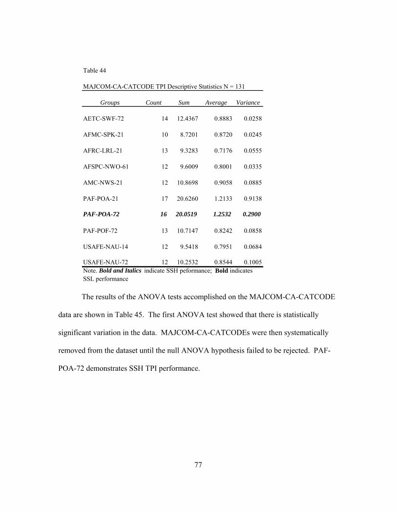
77

Table 44

MAJCOM-CA-CATCODE TPI Descriptive Statistics N = 131


AETC-SWF-72 14 12.4367 0.8883 0.0258

AFMC-SPK-21 10 8.7201 0.8720 0.0245

AFRC-LRL-21 13 9.3283 0.7176 0.0555

AFSPC-NWO-61 12 9.6009 0.8001 0.0335

AMC-NWS-21 12 10.8698 0.9058 0.0885

PAF-POA-21 17 20.6260 1.2133 0.9138

PAF-POA-72 16 20.0519 1.2532 0.2900

PAF-POF-72 13 10.7147 0.8242 0.0858

USAFE-NAU-14 12 9.5418 0.7951 0.0684


The results of the ANOVA tests accomplished on the MAJCOM-CA-CATCODE

data are shown in Table 45. The first ANOVA test showed that there is statistically

significant variation in the data. MAJCOM-CA-CATCODEs were then systematically

removed from the dataset until the null ANOVA hypothesis failed to be rejected. PAF-

POA-72 demonstrates SSH TPI performance.

78

Table 45

MAJCOM-CA-CATCODE TPI One-way ANOVA Results


Between Groups 4.3218 9 0.4802 2.3792 0.0163 1.9581

Within Groups 24.4221 121 0.2018

Total 28.7439 130

Between Groups 2.4455 8 0.3056911 1.614379 0.1292404 2.0269155

Within Groups 20.0717 106 0.1893552

Total 22.51719 114

PAF-POA-72 removed


MAJCOM-CA-CATCODE CPI*TPI Performance

Table 46 shows the descriptive statistics for the CPI*TPI data evaluated for this

research. Consistent with other areas in this research, the CPI*TPI values are above and

below one. This indicates that overall cost and schedule performance are mixed for the

MAJCOM-CA-CATCODEs evaluated in this research.

79

Table 46

MAJCOM-CA-CATCODE CPI*TPI Descriptive Statistics N = 131


AETC-SWF-72 14 12.7916 0.9137 0.0401

AFMC-SPK-21 10 9.4389 0.9439 0.1433

AFRC-LRL-21 13 9.8613 0.7586 0.0681

AFSPC-NWO-61 12 9.6665 0.8055 0.0377

AMC-NWS-21 12 12.6309 1.0526 0.3355

PAF-POA-21 17 22.3315 1.3136 1.2649

PAF-POA-72 16 20.7262 1.2954 0.3029

PAF-POF-72 13 11.1060 0.8543 0.0941

USAFE-NAU-14 12 9.7727 0.8144 0.0310


Table 47 shows the ANOVA test on all of the MAJCOM-CA-CATCODE data

represented in Table 46 resulted in the rejection of the null hypothesis; there is

statistically significant variation present in the data. MAJCOM-CA-CATCODEs were

systematically removed from the data until the null ANOVA hypothesis failed to be

rejected. When AFRC-LRL-21 was removed from the data, the null failed to be rejected;

therefore AFRC-LRL-21 exhibits statistically significant variation from the rest of the

sample.

80

Table 47

MAJCOM-CA-CATCODE CPI*TPI One-Way ANOVA Results


Between Groups 3.1338 8 0.3917 2.8700 0.0063 2.0278

Within Groups 14.3317 105 0.1365

Total 17.46554 113

Between Groups 4.3379 8 0.5422 1.7511 0.0947 2.0244

Within Groups 33.7534 109 0.3097

Total 38.0913 117


AFRC-LRL-21 removed

81

V. Conclusions and Recommendations

Conclusions

The results show that there is statistically significant variation in the cost and

schedule performance of Major Commands (MAJCOMs) and Construction Agents

(CAs). Overall, the AF MILCON program consistently delivers projects that are under

budget; the vast majority of IVs had average Cost Performance Index (CPI) values that

were greater than one. In contrast with the cost performance, most of the IVs were not

able to deliver projects in their allotted time; the vast majority of IVs had average TPI

values that were less than one. The average CPI*TPI values were typically evenly mixed

between above and below one. This indicates that most IVs were exchanging cost

performance for time performance, with varying degrees of success. The results from

this research are summarized in Tables 6A and 6B. Table 48 summarizes the results

associated with research questions one and two; Table 49 summarizes the results for

research question three.

The MAJCOM, CA, and MAJCOM-CA that demonstrates the greatest degree of

cost and schedule success in this research are Pacific Air Forces (PAF), the Alaska

district (POA) of the United States Army Corps of Engineers (USACE), and PAF-POA.

Table 48 shows that either PAF or POA appear as SSH in every category. The team of

PAF and POA are able to consistently deliver projects that are below their respective

budgets and before their respective estimated completion dates. No other MAJCOM,

CA, or MAJCOM-CA combination considered from this dataset has produced similar

results.

82

United States Air Forces in Europe (USAFE) and its primary CAs, the Air Force

Center for Engineering and the Environment (AF) and the European district (NAU) of the

USACE, have produced mixed results. USAFE, AF, and NAU all produced Statistically

Significant High (SSH) CPI performance. However, the CAs NAU and AF, and the

MAJCOM-CAs USAFE-NAU and USAFE-AF, all exhibit Statistically Significant Low

(SSL) TPI performance in the data. Additionally, NAU’s CPI*TPI metrics were also

SSL. In contrast with the PAF and POA results, USAFE, AF, and NAU were not able to

deliver both cost and schedule performance; they were only able to deliver cost

performance.

The SSL TPI performance of some CAs appears to be a major factor in CPI*TPI

performance; the Louisville district (LRL), Mobile district (SAM), and Tulsa district

(SWT) all appear SSL in TPI and CPI*TPI even though they are absent from the SSL

CPI category. Also, Air Force Special Operations Command (AFSOC) SAM and Air

Education and Training Command (AETC) LRL both have SSL TPI and CPI*TPI

metrics. Since the same CAs and MAJCOM-CAs do not display SSL CPI performance,

one explanation might be that time performance is not being traded equally for cost

performance. The Omaha district (NWO) appears in the SSL CPI*TPI metric; this may

indicate that while its CPI and TPI performance individually are not much less than one,

both are likely less than one simultaneously; this effect was demonstrated in Chapter 3,

Figure 3.

83

Table 48

Summary of SSH and SSL performers

MAJCOM CA MAJCOM-CA

SSH CPI performers

PAF

USAFE

AF

NAU

None

SSL CPI performers

None SWF AETC-SWF

SSH TPI performers

ACC None PAF-POA

SSL TPI performers

None AF

LRL

NAU

SAM

SWT

USAFE-AF

AFRC-LRL

USAFE-NAU

AFSOC-SAM

AETC-SWF

SSH CPI*TPI performers

None POA PAF-POA

SSL CPI*TPI performers

None LRL

NAU

NWO

SAM

SAS

SWT

AFRC-LRL

AFSOC-SAM

84

The analysis of MAJCOMs, CAs, and CATCODEs reveals that there is not much

variation in cost and schedule performance due to CATCODE. PAF-POA appears in the

CATCODE data with SSH TPI performance in dormitories, officer quarters, and dining

halls (CATCODE 72). Similarly, AFRC-LRL and SWT re-emerge with SSL CPI*TPI

performance for maintenance facilities (CATCODE 21) and dormitories, officer quarters,

and dining halls (CATCODE 72) respectively. Air Mobility Command makes its only

appearance in these results for SSL TPI performance for maintenance facilities.

85

Table 49

Summary of SSH and SSL performers

CATCODE MAJCOM-

CATCODE

CA-CATCODE MAJCOM-CA-

CATCODE

SSH CPI performers

11 None None None

SSL CPI performers

73

74

None None None

SSH TPI performers

None None POA-72 PAF-POA-72

SSL TPI performers

None AMC-21 SWT-72 None

SSH CPI*TPI performers

None None None None

SSL CPI*TPI performers

None None SWT-72 AFRC-LRL-21

Limitations

One limitation of this research lies in the analysis technique chosen. The

ANOVA test is based on the assumption that the variances of all of the IVs are equal.

The data was not tested to determine if the equal variance assumption was satisfied, nor

86

were any control mechanisms implemented to compensate for unequal variances, if they

exist.

The second limitation of this research is that it measures the efficacy of the

project management effort, not the effectiveness of the projects in satisfying the needs of

their intended customers. This research does not address why the variation that was

discovered exists. The above or SSL performance of the IVs does not indicate why the

particular metric becomes a certain value. Also, even though time performance is

calculated, the metric does not indicate if the project was delivered fast enough to support

the mission for which it was intended. For example, a new runway project is completed

on time according to the project documents; it achieved a TPI score of one.

Unfortunately, the aircraft the runway was designed to support arrived one year before

the runway project was completed; this result degraded the mission but is not captured by

the TPI metric as calculated in this research.

The third limitation of this research is that the cost and schedule metrics were

relative in nature. The CPI measured how closely projects came to meeting their budgets

and schedules, but the budgets and schedules are set by the MAJCOMs and CAs. There

are no references to how much facilities should cost or how long they should take to

construct compared to industry standards for similar activities.

Contributions

This research sought to find statistically significant variation in cost and schedule

performance of AF Military Construction (MILCON) projects. Historical records of cost

and schedule performance were analyzed using the analysis of variance (ANOVA) test to

87

determine if statistically significant variation existed among MAJCOMs, CAs,

CATCODES, or combination of these three IVs.

This research makes a contribution to the AF by objectively and systematically

analyzing the cost and schedule performance of the AF MILCON program. This research

can be used by AF project managers to investigate statistically significant variation in

performance, share best practices and lessons learned across the AF. The academic

contribution of this research lies in applying Earned Value Analysis techniques to actual

project data.

Opportunities for Future Research

Future research could be accomplished to answer the “why” questions generated

by this research. Case study research could investigate why PAF-POA consistently

generates SSH CPI and TPI metric performance. Case study research could also be done

to examine why USAFE consistently generates SSH CPI performance, but SSL TPI

performance with two different construction agents. Lastly, further quantitative research

could be done on this dataset to compare other measures of cost and schedule

performance that take into account industry standards for construction costs and

timelines.

88

Bibliography

America's aging infrastructure is not a joke (2007). Engineering News Record, 259(5),

68.

Anbari, F., T., (2003). Earned Value Project Management Method and Extensions.

Project Management Journal, 34(4), 12.

Arellano, Hector A. (1995). Analysis of Contract Modifications on Military Construction

(MILCON) Projects Administered by the U.S. Naval Facilities Engineering

Command. (MS, The University of Texas at Austin).

Ashley, D. B., Lurie, C. S., & Jaselskis, E. J. (1987). Determinants of construction project

success. Project Management Journal, 18(2), 69.

Baker, D., C., Murphy, D., C., & Fisher D., (1988) Factors Affecting Project Success.

Project Management Handbook, New York, Van Nostrand Reinhold.

Chan, Albert P. C. (Dept. of Building, Hong Kong Polytechnic Univ.). (2002).

Framework of success criteria for design/build projects. Journal of Management in

Engineering, 18(3), 120.

Dvir, D., Raz, T., & Shenhar, A., J. (2003). An empirical analysis of the relationship

between project planning and project success. International Journal of Project

Management, 21(2), 89-96.

Department of the Air Force. Planning and Programming Military Construction

(MILCON) Projects. AFI32-1021. Washington: HQ USAF, October 2003.

Department of the Air Force. The United States Air Force Project Manager’s Guide for

Design and Construction. Washington: HQ AFCEE, June 2000.

89

Department of the Air Force. Design And Construction Standards And Execution Of

Facility Construction Projects. AFI32-1023. Washington: HQ USAF, July 1994.

de Wit, A. (1986). Measuring project success: an illusion. 1986 Proceedings Of The

Project Management Institute, Drexel Hill, Pa., 13-21.

Freeman, M., & Beale, P. (1992). Measuring project success. Project Management

Journal, 23(1), 8.

Gaddis, P., O. (1959) The Project Manager. Harvard Business Review, 37(3), 89.

Gibson, G. E. Jr., (1994) “Analysis of Pre-Project Planning Effort and Success Variables

for Capital Facility Projects” Austin, TX: Construction Industry Institute.

Griffith, A. F., Gibson, G. E., Hamilton, M. R., Tortora, A. L., & Wilson, C. T. (1999).

Project success index for capital facility construction projects. Journal of

Performance of Constructed Facilities, 13(1), 39.

Jha, K., N., Iyer, K., C. (2007). Commitment, Coordination, Competence, and the Iron

Triangle. International Journal of Project Management, 25, 527-540.

Hughes, S. W., Tippett, D. D., & Thomas, W. K. (2004). Measuring project success in

the construction industry. Engineering Management Journal, 16(3), 31-37.

McClave, J., T., Benson, P., G., & Sincich, T., (2005) Statistics for Business and

Economics (9th ed.): Upper Saddle River, NJ. Pearson Prentice Hall.

Meredith, J. R., & Mantel, S., J., (2000) Project Management A Managerial Approach

(4th ed.): New York: John Wiley & Sons.

Slevin, D. P., & Pinto, J. K. (1986). The project implementation profile: New tool for

project managers. Project Management Journal, 17(4), 57.

REPORT DOCUMENTATION PAGE Form Approved OMB No. 074-0188

The public reporting burden for this collection of information is estimated to average 1 hour per response, including the time for reviewing instructions, searching existing data sources, gathering and maintaining the data needed, and completing and reviewing the collection of information. Send comments regarding this burden estimate or any other aspect of the collection of information, including suggestions for reducing this burden to Department of Defense, Washington Headquarters Services, Directorate for Information Operations and Reports (0704-0188), 1215 Jefferson Davis Highway, Suite 1204, Arlington, VA 22202-4302. Respondents should be aware that notwithstanding any other provision of law, no person shall be subject to an penalty for failing to comply with a collection of information if it does not display a currently valid OMB control number. PLEASE DO NOT RETURN YOUR FORM TO THE ABOVE ADDRESS. 1. REPORT DATE (DD-MM-YYYY)

27-03-2008 2. REPORT TYPE

Master’s Thesis 3. DATES COVERED (From – To)

March 2007 – March 2008 5a. CONTRACT NUMBER

5b. GRANT NUMBER

4. TITLE AND SUBTITLE An Analysis Of Construction Cost And Schedule Performance

5c. PROGRAM ELEMENT NUMBER

5d. PROJECT NUMBER 5e. TASK NUMBER

6. AUTHOR(S) Beach, Michael J., Major, USAF

5f. WORK UNIT NUMBER

7. PERFORMING ORGANIZATION NAMES(S) AND ADDRESS(S) Air Force Institute of Technology Graduate School of Engineering and Management (AFIT/EN) 2950 Hobson Way, Building 640 WPAFB OH 45433-8865

8. PERFORMING ORGANIZATION REPORT NUMBER AFIT/GEM/ENV/08-M02

10. SPONSOR/MONITOR’S ACRONYM(S)

9. SPONSORING/MONITORING AGENCY NAME(S) AND ADDRESS(ES) This space intentionally left blank

11. SPONSOR/MONITOR’S REPORT NUMBER(S)

12. DISTRIBUTION/AVAILABILITY STATEMENT APPROVED FOR PUBLIC RELEASE; DISTRIBUTION UNLIMITED.

13. SUPPLEMENTARY NOTES 14. ABSTRACT Cost and schedule performance are widely accepted in the literature and in industry as effective measures of the success of the project management effort expended. Earned Value Analysis (EVA) offers many metrics to objectively measure cost and schedule performance of many different types of projects. The author utilized EVA to objectively measure the cost and schedule performance of completed United States Air Force (AF) Military Construction (MILCON projects from 1990 to 2005. The impact of Major Command (MAJCOM), Construction Agent (CA), and facility type (CATCODE) and the combination of these variables on the EVA metrics of Cost Performance Index (CPI), Time Performance Index (TPI), and CPI*TPI were evaluated. The CPI results indicate that AF MILCON projects are typically executed either on or below their respective budgets. Conversely, the TPI results indicate that AF MILCON projects typically take more time than expected for construction. The CPI*TPI results indicate that the AF MILCON projects in this study typically exchange higher cost performance for lower time performance. However, when CPI and TPI are given equal weight, the sacrifice made in time performance is greater than the benefit gained in cost performance.

15. SUBJECT TERMS Cost, Schedule, Earned Value Analysis, Iron Triangle, Project Management, Construction Management, MILCON 16. SECURITY CLASSIFICATION OF:

19a. NAME OF RESPONSIBLE PERSON Sonia E. Leach, Maj, USAF

a. REPORT

U

b. ABSTRACT

U

c. THIS PAGE

U

17. LIMITATION OF ABSTRACT

UU

18. NUMBER OF PAGES

104

19b. TELEPHONE NUMBER (Include area code) (937) 255-6565, ext 7390 ([email protected])

Standard Form 298 (Rev. 8-98) Prescribed by ANSI Std. Z39-18

AIR FORCE INSTITUTE OF TECHNOLOGY · an analysis of construction cost and schedule performance...

Documents

Transcript of AIR FORCE INSTITUTE OF TECHNOLOGY · an analysis of construction cost and schedule performance...