sensors

Article

Air-Coupled and Resonant Pulse-EchoUltrasonic Technique

Tomás Gómez Álvarez-Arenas * and Jorge Camacho

Instituto de Tecnologías Físicas y de la Información (ITEFI), Spanish National Research Council (CSIC),

28006 Madrid, Spain; j.camacho@csic.es

* Correspondence: t.gomez@csic.es

Received: 15 April 2019; Accepted: 9 May 2019; Published: 14 May 2019�����������������

Abstract: An ultrasonic, resonant, pulse-echo, and air-coupled nondestructive testing (NDT) technique

is presented. It is intended for components, with regular geometries where it is possible to excite

resonant modes, made of materials that have a high acoustic impedance (Z) and low attenuation

coefficient (α). Under these conditions, these resonances will present a very large quality factor

(Q) and decay time (τ). This feature is used to avoid the dead zone, produced by the echo coming

from the first wall, by receiving the resonant echo from the whole specimen over a longer period

of time. This echo is analyzed in the frequency domain to determine specimen resonant frequency,

which can be further used to determine either velocity or thickness. Using wideband air-coupled

transducers, we tested the technique on plates (steel, aluminum, and silicone rubber) by exciting

the mode of the first thickness. As expected, the higher the Z and the lower the α, the better the

technique performed. Sensitivity to deviations of the angle of incidence away from normal (±2◦) and

the possibility to generate shear waves were also studied. Then, it was tested on steel cylindrical

pipes that had different wall thicknesses and diameters. Finally, the use of this technique to generate

C-Scan images of steel plates with different thicknesses was demonstrated.

Keywords: air-coupled ultrasound; ultrasonic NDT; air-coupled transducers; air-coupled pulse-echo;

pipe NDT; pipe wall gauge

1. Introduction

Air-coupled ultrasound is a convenient method for material characterization and nondestructive

testing (NDT) when conventional techniques based on water immersion, local immersion, gel coupling,

or dry coupling cannot be used. There can be different reasons for the need to use air-coupled techniques.

In the case of material characterization, examples are commonly found in the determination of elastic

and viscoelastic constants. Examples are also found in determining the microstructural properties of

porous, open-pore materials or soluble materials, where the use of coupling fluids must be avoided.

In other cases, coupling fluids cannot be used because they can potentially contaminate or modify

the material. Examples commonly appear in the food industry and in the study of biological tissues,

synthetic membranes, and porous solids. Similarly, air-coupled ultrasound can be a very interesting

solution for NDT (see [1] for an early review in this field). Examples correspond to cases where the

potential penetration of fluids within the testing piece is to be avoided. In other cases, air-coupled

techniques can be used to replace water-jet or water immersion systems when saving water, time,

and/or energy consumption is advantageous. Finally, air-coupled techniques can be thoroughly used

to generate and receive guided waves in solid structures. This may present some advantages in order

to test large specimens or those that present difficult access points. Use of air-coupled ultrasound for

Lamb waves in metal plates was first demonstrated in 1973 [2]. Since then, Lamb waves have been

extensively used for different materials, including fiber-reinforced polymer composites [3].

Sensors 2019, 19, 2221; doi:10.3390/s19102221 www.mdpi.com/journal/sensors

Mor

e in

fo a

bout

this

art

icle

: ht

tp://

ww

w.n

dt.n

et/?

id=

2448

1

Sensors 2019, 19, 2221 2 of 18

The main problem of air-coupled ultrasound is the huge impedance mismatch between air and

any solid material. This impedance mismatch gives rise to a very high reflection coefficient (R) at

any air/solid interface (R ≈ 1). Thus, only a very small portion of incident energy is transmitted

(T ≈ 0, where T is the transmission coefficient), which leads to very low-amplitude transmitted signals

and poor signal-to-noise ratio (SNR) values. This same problem also affects piezoelectric air-coupled

transducers, which make the situation even more difficult. In most cases, there is also a significant

difference between the ultrasonic velocity in the air and in the solid material, which produces a strong

refraction at the interfaces; consequently, the limit angle will appear at quite low values.

Despite all these problems, and because of the continuous improvement in air-coupled

transducers [4], electronics, signal-processing-like coded excitation [5,6], and inspection techniques,

there are good records of successful applications in different fields and by different groups [7].

One of the consequences of having R ≈ 1 is that energy will be strongly confined within both air

cavities and solid pieces. Depending on the air cavity, solid piece, and ultrasonic field geometry this can

lead to the appearance of strong resonances. Thickness resonances in plates at normal incidence can be

used as a way to boost the level of transmitted energy through the plate, especially for high-impedance

materials [8]. Later, use of these resonances was proposed by Hutchins and coworkers as a means

to determine velocity in the material if thickness was known [9,10] and, alternatively, to determine

the thickness of metal plates [11]. Later advances in this sense included the use of oblique incidence

to obtain information about shear properties [12,13], the use of both magnitude and phase spectra to

obtain simultaneous information on thickness and velocity [14], and the analysis of layered composites

using resonance imaging [15].

Given that R ≈ 1, air-coupled ultrasound can be well-used in pulse-echo mode to study the

roughness of surfaces, to produce an image of the surface profile [16,17], and as a scanner for Braille [18].

One of the main limitations of air-coupled ultrasound in studying the inner volume of a solid is that it

is impossible, in most practical situations, to operate in pulse-echo mode, although this possibility has

been considered since the early developments of this technique [19]. This is because the echo coming

from the back surface is very small and appears buried within the echo reflected from the front surface.

The only chance to detect this low-amplitude, back wall echo is to avoid the dead zone produced

by the front wall echo. This implies that we must wait until its influence disappears, a time we call

tDZ. Considering that, in most air-coupled applications, low frequencies (<0.5 MHz) and relatively

narrowband transducers are commonly used, tDZ can be quite large; this limits the applicability of

the technique to quite thick plates. Unfortunately, this imposes another restriction, as the attenuation

coefficient in the material must be low enough. In addition, distance between the transducer and

the front plate surface must be large enough so that the reverberations within the air column do not

overlap with the back wall echo. This normally implies a long propagation path in the air, which

introduces some extra losses from attenuation in the air and beam diffraction. Exceptions appear when

tDZ is relatively shorter; this is the case in low-impedance solids (porous or soft solids) or when the

pressure in the air is elevated (pressurized pipes) [20,21].

An alternative can be the use of two different transducers in pitch–catch mode, but the dead zone

does not disappear completely, and the technique becomes more difficult to implement since two

different transducers are involved [22]. If oblique incidence is considered, accuracy in the control of

angle and location is critical in order to separate specular reflection from the front surface and back

wall echoes originating from longitudinal and shear waves, which also requires accurate knowledge of

the longitudinal and shear wave velocities in the material.

For plates made of high-impedance (Z) and low-attenuation coefficient (α) materials (like most

metals, glass, and some ceramics) the Q-factor of the thickness resonance can be very large, which

means that the time the signal keeps reverberating within the material can be very large as well. The

proposed idea in this paper is to launch a wideband, airborne, ultrasonic pulse towards a solid material

(with high Z and low α and at normal incidence) in order to excite a high-Q resonance of the solid

piece. Then, the same transducer is used to receive the resonant echo generated by the solid. Because

Sensors 2019, 19, 2221 3 of 18

of the high Q-factor of the resonance in the test object, this can be done after a long enough time so that

the front wall echo and its reverberations within the air gap have disappeared. Clearly, the transducer

frequency band must encompass at least one of the resonant frequencies of the solid specimen so that

the pulse is able to generate resonances in it.

The objective of this paper is twofold: (i) to test the feasibility of this approach in plates (normal

incidence) and cylindrical pipes (quasi-normal incidence) made of different materials, and (ii) to test the

possibilities of this technique to generate a C-Scan image, based on the value of the resonant frequency

of the plate/pipe, so that the thinning of plate or pipe walls can be determined for NDT applications.

2. Materials and Methods

2.1. Methods

The proposed methodology consisted of selecting a set of plates and pipes made of different

materials and with different thicknesses. First, they were measured using a conventional air-coupled

through-transmission (TT) configuration using normal incidence, wideband transducers, and spectral

analysis of the transmission coefficient with the purpose to determine the frequency location of the

first thickness resonance (fres). For plates at normal incidence, fres is derived directly from the plate

thickness (t) and the phase velocity of ultrasound longitudinal waves in the material (v) by:

fres =v

2t. (1)

Other parameters of interest for this study included the duration of the reverberations within the

material, as this provided an initial estimation of the feasibility of the proposed resonant pulse-echo

procedure. This was related with the quality factor of the resonance (Q-factor or Q), which was

determined by Z of the solid specimen and the air, α of the solid, and other factors like the plate

surface roughness, the presence of plate imperfections (lack of homogeneity of the solid or lack of

parallelism between both plate surfaces), and any deviation of the beam away from normal incidence.

It is defined by:

Q =fres

∆ f∣

∣

∣

6dB

, (2)

where ∆ f∣

∣

∣

6dBis the width of the resonance peak at 6 dB below the maximum value. The Q factor is

related to the decay time (τ) by:

τ =Q

π fres. (3)

After the measurement in TT mode, we switched to the pulse-echo (PE) configuration, and we

took the Fast Fourier Transform (FFT) of the signal for a temporal window located at t0 > tDZ to verify

if there was still some measurable contribution of the reverberations in the plate from the thickness

resonances. This was done by comparing the frequency components of the FFT with that measured

in the TT configuration. In some cases, we took different windows at different t0 values to check the

integrity of the results. This process was repeated for samples having different thicknesses, made of

different materials, and with different values of the Q factor, τ, and fres.

Then, the influence of the angle of incidence was tested using steel plates with the purpose to

estimate how critical the transducer–plate alignment was and if it was possible to generate and observe

shear waves. This was done by measuring variations in the amplitude of the thickness resonance peak,

measured in pulse-echo mode, when the angle of incidence varied from −2 to 2 degrees.

Once the feasibility, the robustness, and the limits of the technique were tested with plates, we

followed the same procedure with two different cylindrical pipes made of two different steels and with

different thicknesses.

Finally, we performed a C-Scan image using the proposed PE-resonant technique of steel plates

with different thicknesses and used the value of the resonant frequency to generate a C-Scan image.

Sensors 2019, 19, 2221 4 of 18

2.2. Experimental Methods and Setups

All the results presented in this work were obtained using wideband, high-sensitivity air-coupled

transducers with a center frequency of 0.25 MHz, a −20 dB bandwidth (60%), a circular aperture

(diameter = 25 mm), and a flat radiating surface that was designed and built in our research group [23].

These transducers could be used both in TT or PE configurations. Signals in the time domain and

sensitivity (SNS) in the PE mode are shown in Figure 1. For the reflector we used a brass block, and

distance to reflector was 45 mm. SNS is obtained by:

SNS(dB) = 20log10

∣

∣

∣FFT(VRx)∣

∣

∣

∣

∣

∣FFT(VTx)∣

∣

∣

, (4)

where V is the electrical voltage measured at transducers terminals, and FFT denotes the fast Fourier

transform. The temporal window for the FFT was square, with a duration (∆t) 200 µs, and was located

at t0 = 0 µs and t0 = 200 µs for FFT(VTx) and FFT(VRx), respectively.

‒

𝑆𝑁𝑆 𝑑𝐵 = 20𝑙𝑜𝑔 | || |FFT 𝑉 FFT 𝑉

(a) (b)

Figure 1. Transducer impulse response in the time domain VRX (a) and sensitivity frequency band SNS

(b) in pulse-echo (PE) mode. The FFT was obtained from VRX in a temporal window between 250 and

450 µs.

The response shown in Figure 1 was obtained by driving Tx (VTX) with a negative semicycle

of square pulses, amplitude of 100 V, and a frequency of 250 kHz, provided by an Olympus 5077PR

pulser-receiver (Tokyo, Japan). Signals generated at Rx (VRX) were sent to the receiver stage of the

5077PR. The gain was set to 0 dB with no filtering, and the signal was transferred to a digital oscilloscope

(Tektronix 5072, Beaverton, OR, USA) to digitize the signal, display it, store it, and extract it to the FFT.

2.2.1. Through-Transmission (TT)

Transducers and sample configurations for both plates and pipes are shown in Figure 2.

An Olympus 5077 (Tokyo, Japan) pulser-receiver was used to drive Tx with a square semicycle

(pulse amplitude: 400 V, pulse center frequency: 250 kHz, and pulse repetition frequency (PRF): 100 Hz)

and to amplify and filter the signal provided by Rx (gain: +59 dB, low-pass filter: 10 MHz). It was

then transferred to the digital scope (Tektronix 5072, Beaverton, USA, bandwidth limit set to 20 MHz),

which was triggered by the synchronism signal provided by the 5077PR. The scope digitized the signal

and then was loaded into MATLAB (Mathworks, Natick, MA, USA) for further processing. Tx – Rx

separation was typically 120 mm. Normal incidence was used for plates, while for cylindrical pipes,

transducers were aligned along the radial direction (see Figure 2).

Sensors 2019, 19, 2221 5 of 18

Figure 2. Transducers and sample configurations in through transmission measurements: (a) plate and

(b) cylindrical pipe.

2.2.2. Pulse-Echo (PE)

Transducers and sample configurations are shown in Figure 3. The same configuration as before

was employed, with the exceptions that now we operated in PE mode and that a lower pulse repetition

frequency (PRF) was used (25 Hz). The trigger signal was provided by an Agilent 3320A (Santa Clara,

CA, USA) arbitrary waveform generator; this trigger signal was employed to trigger both the 5077

pulser-receiver and the oscilloscope.

Figure 3. Transducers and sample configurations in pulse measurements: (a) plate, (b) cylindrical pipe,

(c) C-Scan of three different steel disks, and (d) cylindrical pipe with stepped pipe wall thickness.

2.2.3. Resonant PE C-Scan Images

The configuration of Figure 3c was used to scan three stainless steel disks of different thicknesses

(10.0 mm, 11.0 mm, and 12.0 mm) placed on a planar surface. A DIS-300 automated scanner and an

Air-Scope ultrasound system, both from Dasel S.L. (Madrid, Spain), were used to acquire reflection

signals from a single transducer located at a distance of 40 mm. A grid of 50 mm × 125 mm was

scanned in 1 mm steps (X and Y directions). The encoders of the scanning system were used to

trigger pulse-echo acquisitions of 7 ms windows, which were delayed 4 ms from the excitation signal.

Sensors 2019, 19, 2221 6 of 18

Acquired data were loaded in Matlab, and the center frequency of each signal was estimated by FFT in

a temporal window at t0 > tDZ. Finally, a C-Scan was generated by color coding the resonant frequency

in Hz.

2.3. Materials

Descriptions of the main properties of the samples employed for the study are shown in Tables 1

and 2. The diameters of the steel pipes were selected to be much larger than the transducer’s diameter

(25 mm) so that we were close to quasi-normal incidence. The wall of the 305 mm diameter steel pipe

was initially uniform and equal to 12.59 ± 0.4 mm; it was reduced along three 40 mm-wide bands

using a lathe (see Figure 3d and Table 2) to generate four sections with different thicknesses. In these

cases, the lathed surfaces presented a larger roughness that certainly affected the amplitude of the

resonant mode of the pipe wall in these sections. Finally, three steel discs of 36 mm diameter (same

steel as in Table 1) and different heights (10.0 mm, 11.0 mm, and 12.0 mm) were used for the C-Scan

(see Figure 3c).

Table 1. Circular plates used for the study: materials and thicknesses.

Material Thickness (mm) Diameter (mm)

Stainless steel

10.0 ± 0.05 36

11.0 ± 0.05 36

12.0 ± 0.05 36

Aluminum 13.5 ± 0.05 55

Silicone rubber 2.0 ± 0.02 40

Table 2. Pipes used for the study: material pipe diameters and wall thicknesses.

Material Diameter/Wall Thickness (mm)

Steel (1)

305/10.30 ± 0.2

305/11.16 ± 0.3

305/11.86 ± 0.4

305/12.59 ± 0.4

Steel (2) 324/13.10 ± 0.2

3. Results

3.1. Through-Transmission

For the steel plates in Table 1, and because of the very large Z mismatch between the air (~420 Rayl)

and the steel as well as the expected low α in the steel plate at the resonant frequency, we expected R ≈ 1

and very large values for both Q-factor and τ. As an example, transmitted signal and FFT measured in

the 11 mm steel plate are shown in Figure 4. The transmitted signal in the time domain was much

larger than the incident one (Figure 1). This was because the reverberations within the plate were

almost free of damping and gave rise to a strong and sharp thickness resonance. FFT of the signal

revealed that fres = 247.06 kHz, Q > 6200, and τ > 8 ms. Then, according to Equation (1), v = 5435 m/s;

considering ρ = 7800 kg/m3, then Z = 42.4 MRayl, and T = 3.72 × 10−5. Actually, the decay time of

the reverberations in the plate was so long that it was possible to place a 5 ms temporal rectangular

window, at a time called t0, where t0 = 42 ms, and get the same frequency content of the signal when a

similar window was located at t0 = 0.02 ms (see Figure 4) with a 19 dB loss in the peak amplitude of

the FFT. Similar results were obtained for the other stainless steel plates. Table 3 shows the measured

thickness resonant frequencies for all cases. From Equation (1) we knew that the ratio of the resonant

Sensors 2019, 19, 2221 7 of 18

frequencies (f 1 and f 2) of two plates of the same material, but with different thicknesses (t1 and t2),

was: f 1/f 2 = t2/t1. In this case, this relationship was upheld, as we had t2/t1 = 1.09, 1.1, and 1.2, and the

measured ratios of the resonant frequencies were f 1/f 2 = 1.088, 1.101, and 1.198, respectively.

α𝑓−

α𝑓−

α

Figure 4. Through-transmission in the 11 mm-thick stainless steel plate. Top: signal in the time domain.

Center: FFT modulus of the signal within window (1). Bottom: FFT modulus of the signal within

window (2).

Table 3. Through-transmission resonant frequency.

Sample Material Thickness (mm) Resonant Frequency (kHz)

PlateStainless Steel

10.0 ± 0.05 272.0

11.0 ± 0.05 247.0

12.0 ± 0.05 227.1

Aluminum 12.5 ± 0.05 231.0

Silicone rubber 2.0 ± 0.02 241.0

Steel Pipe(1)

10.3 ± 0.2 1 276

11.16 ± 0.3 1 257

11.86 ± 0.4 1 243

12.59 ± 0.4 227.5

(2) 13.1 ± 0.2 221.5

1 Lathed inner surface.

Compared with stainless steel plates, a lower Q value for the first thickness resonance was

expected in aluminum plates because of the lower value of Z and a larger α. Results for a 13.5 mm-thick

plate are shown in Figure 5. fres = 231 kHz, Q > 900, and τ > 1.2 ms. According to Equation (1) and

considering ρ = 2700 kg/m3, then v = 6237 m/s, and Z = 16.7 MRayl; hence, T = 9.8 × 10−5. That is, a

much more attenuated resonance (compared with the previous case) was obtained. In spite of lower Q

Sensors 2019, 19, 2221 8 of 18

and τ values, it was still possible to take a delayed (t0 = 7 ms) 1 ms-long temporal window and obtain

the same frequency content of the signal as when a nondelayed window was used. The amplitude

reduction in the FFT peak produced by delaying the window was now larger than in the case of steel

plates (even considering that now t0 was also much smaller) at 25 dB.

Figure 5. Through-transmission in the 13.5 mm-thick aluminum plate. Top: signal in the time domain.

Center: FFT modulus of the signal within window (1). Bottom: FFT modulus of the signal within

window (2).

For a silicone rubber plate, and because of the even lower Z and larger α of this material, the Q

factor and the decay time of the thickness resonance were expected to be much lower. These features

are shown in Figure 6: fres = 241.7 kHz, Q ≈ 198, and τ ≈ 0.26 ms. Hence, v = 967 m/s, and considering

ρ = 900 kg/m3, then Z = 0.87 MRayl, R = 0.9981, and T = 1.89 × 10−3. However, even in this case it was

possible to place a 1 ms window (delayed 3 ms) and get the same frequency components of the signal,

although the signal amplitude decay (46 dB) was much larger than in the previous cases.

Finally, for a steel pipe, and in spite of the high Z and low α of the material, a much more damped

resonance than in the plate specimens was expected. This was because a mode conversion (longitudinal

to shear) produced by the non-normal incidence was present. And as the acoustic field reverberated

within the pipe wall, the propagation direction was modified, and a reduced portion of the acoustic

beam went back into the transducer. One example is shown in Figure 7, where Q = 228, while for a

steel plate Q > 6200. In spite of this larger damping, it was still possible to place a 1 ms window at

t0 = 3.5 ms and obtain the same signal frequency content as for a window located at t0 = 0.1 ms; the loss

in the peak amplitude of the FFT was much lower than in the case of the silicone rubber plate at 13 dB.

Sensors 2019, 19, 2221 9 of 18

Figure 6. Through-transmission in the 2 mm-thick rubber plate. Top: signal in the time domain. Center:

FFT modulus of the signal within window (1). Bottom: FFT modulus of the signal within window (2).

Figure 7. Through-transmission for the 324 mm diameter and 13.1 mm-thick steel pipe. Top: signal in

the time domain. Center: FFT modulus of the signal within window (1). Bottom: FFT modulus of the

signal within window (2).

Sensors 2019, 19, 2221 10 of 18

Results (materials, sample geometry, thickness, and resonant frequency) for through-transmission

are summarized in Table 3.

3.2. Pulse-Echo

3.2.1. Plates

As an example of the received signal in PE configuration, Figure 8 shows the result for the 11 mm

steel plate (same plate as in Figure 4) using a PRF = 50 Hz (a weakly damped monochromatic signal

produced by the high-Q thickness resonance in the steel plate). tDZ expanded up to tDZ ≈ 5 ms.

As amplitude scale was set to measure the signal after tDZ, the echo from the front face and the

reverberations in the air cavity between transducers appeared saturated. Placing a 2 ms temporal

window at t0 > tDZ and extracting the FFT, the obtained resonant frequency was the same as that

obtained using the TT configuration (Figure 4). Moreover, it was possible to delay this temporal

window up to t0 = 17 ms and obtain the same frequency, with a reduced loss in the peak amplitude of

only 4 dB (Figure 8).

𝑓 𝑓 𝑓

Figure 8. Pulse-echo; 11 mm-thick stainless steel plate. Top: signal in the time domain. Center: FFT

modulus of the signal within window (1). Bottom: FFT modulus of the signal within window (2).

Using this same procedure, we measured resonant frequency and amplitude of the FFT peak

for the rest of the samples in Tables 1 and 2. Figure 9 compares the FFT of the signal received in PE

configuration from the three stainless steel plates (10, 11, and 12 mm) using a square temporal window

for the FFT located at t0 = 10 ms and a length ∆t = 7 ms. Table 4 shows all measurements using a

square temporal window for the FFT of the same length or duration, given by ∆t, where: ∆t = 2 ms,

is located just after tDZ (which varied for different samples).

Sensors 2019, 19, 2221 11 of 18

𝑓 𝑓 𝑓Figure 9. FFT modulus of the signal received from the three stainless steel plates in pulse-echo.

Red ( fres = 227.5 kHz): 12 mm-thick plate, Green ( fres = 247.0 kHz): 11 mm-thick plate, and Blue

( fres = 272.0 kHz): 10 mm-thick plate. FFT window: t0 = 10 ms, ∆t = 7 ms.

Table 4. Pulse-echo resonant frequency and peak amplitude.

Sample Material Thickness (mm)Resonant

Frequency 2 (kHz)Peak Value of the

Modulus of the FFT 2

PlateStainless Steel

10.0 ± 0.05 272.0 1197

11.0 ± 0.05 247.0 1830

12.0 ± 0.05 227.1 910

Aluminum 12.5 ± 0.05 231.0 56.1

Silicone rubber 2.0 ± 0.02 241.5 53.2

PipeSteel (1)

10.3 ± 0.2 1 – –

11.16± 0.3 1 257.1 17.0

11.86 ± 0.4 1 242.3 16.0

12.59 ± 0.4 227.5 40.5

Steel (2) 13.1 ± 0.2 221.7 14.0

1 Lathed inner surface; 2 using a 2 ms rectangular window located after tDZ.

Resonant frequencies of the different samples obtained in PE mode (Table 4) agreed well with

resonant frequencies measured in TT mode (Table 3). As expected from TT results, the largest signal

amplitudes were obtained for the steel plates, while peak amplitudes in aluminum and silicone rubber

plates were much smaller. Although peak amplitudes were similar in these two cases, there were

some significant differences that were appreciated in Figures 10 and 11. In the case of the silicone

rubber plate (Figure 11), and because of the shorter τ (τ = 0.26 ms), the only way to measure the

resonant frequency was to locate the temporal window for the FFT as close to tDZ (3 ms) as possible,

otherwise the reverberations in the plate disappeared. Unfortunately, as we got closer to tDZ, the noise

level increased, and some other frequencies appeared (resulting from the transducer band and the

reverberations within the air cavity). On the contrary, for the aluminum plate (Figure 10) τ = 1.2 ms.

We could further delay the temporal window (to = 8 ms) and still have a relatively larger amplitude of

the resonance peak. Only for the steel (1) pipe with a thickness 10.3 mm was no thickness resonance

observed (Table 4). This was attributed to the larger roughness of the lathed wall in this section and to

the fact that the expected resonant frequency was 276 kHz; at this frequency, the transducer sensitivity

was slightly smaller (Figure 1).

Sensors 2019, 19, 2221 12 of 18

Figure 10. Pulse-echo; 13.5 mm-thick aluminum plate: signal in the time domain (top) and FFT

modulus of the signal within the indicated window (bottom).

α

𝑓 𝑣2𝑡 𝑛

Figure 11. Pulse-echo; 2 mm-thick silicone rubber plate: signal in the time domain (top) and FFT

modulus of the signal within the indicated window (bottom).

3.2.2. Pipes

For the steel pipes, and because of the geometrical reasons previously mentioned, the amplitude

of the resonance peak was much smaller than in the case of plates. The larger amplitude corresponded

to the steel (1) pipe in the section that was not lathed. This could be explained by the larger surface

roughness present in the lathed sections and the negative influence of this roughness on the resonance

condition. Figure 12 shows the measured response of the 305 mm diameter and 12.59 mm-thick steel

(1) pipe. As in Figure 11, Figure 12 shows that selecting t0 close to tDZ resulted in an increase of the

background noise in the FFT. However, and thanks to the larger value of Z and lower value of α, τ

was larger. It was possible to use larger values of t0 with a moderate decrease in the amplitude of the

resonance peak while eliminating most of the noise from other frequency components. In addition,

Sensors 2019, 19, 2221 13 of 18

Figure 12 revealed the presence of a much smaller peak that did not seem to be affected by the location

of the FFT window, which appeared at 254 kHz. If we assume that this peak corresponds to the

second-order thickness resonance of the shear wave, the velocity of this wave can be obtained from [24]:

f nres ≈

v

2tn (5)

where n = 1, 2, . . . is the order of the resonance, which gives vt = 3200 m/s for n = 2, and it is consistent

with known values for steel and with the previously measured longitudinal velocity.

Figure 12. Pulse-echo; 12.59 mm-thick stainless steel pipe. Top: signal in the time domain. Center: FFT

of the signal within window (1). Bottom: FFT of the signal within window (2).

3.2.3. Influence of the Angle of Incidence

Finally, we investigated the influence of possible misalignments between the transducer and

plate on the amplitude of the resonance peak. To have an initial estimation of how significant this

effect can be, we used the 10 mm-thick steel plate and deviated the angle of incidence from 0◦ (which

corresponds to normal incidence) up to ±2◦ in steps of 0.5◦. The variation in peak amplitude relative

to the peak amplitude at normal incidence is shown in Figure 13. Differences at constant angles were

due to the measurement noise.

When incidence deviated from normal incidence, the amplitude of the resonance peak was

expected to decrease. This was produced by the deviation of the ultrasonic beam from the transducer

aperture as well as by the mode conversion and generation of shear waves in the plate surfaces.

Appearance of shear waves was suggested to explain the additional peak observed in stainless steel

pipes (Figure 12). This was better observed in this case thanks to the flat surfaces of the plate samples.

Figure 14 shows the amplitude of the FFT in PE mode for the 11 mm-thick steel plate using a square

temporal window, where t0 = 20 ms, ∆t = 19 ms, and for two different values of the deviation of the

angle of incidence away from normal incidence (θ): 0◦ and 1◦. The additional peak at 252.78 kHz for

θ = 1◦ was due to the second-order resonance of the shear wave (vs. ≈ 2780 m/s).

Sensors 2019, 19, 2221 14 of 18

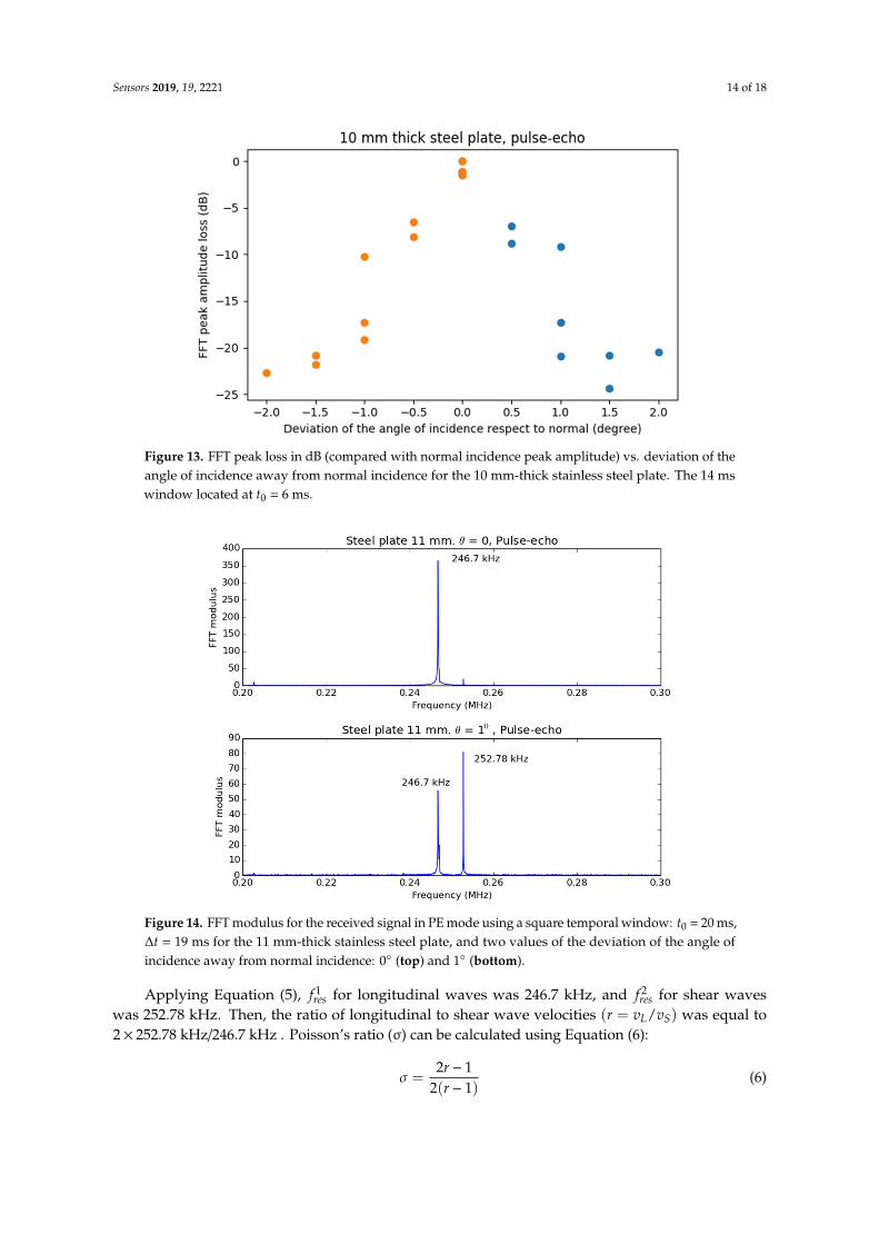
Figure 13. FFT peak loss in dB (compared with normal incidence peak amplitude) vs. deviation of the

angle of incidence away from normal incidence for the 10 mm-thick stainless steel plate. The 14 ms

window located at t0 = 6 ms.

θθ

𝑓 𝑓𝑟 = 𝑣 𝑣⁄2 252.78 𝑘𝐻𝑧 246.7 𝑘𝐻𝑧⁄ σ𝜎 = 2𝑟 12 𝑟 1σ

σσ σ

Figure 14. FFT modulus for the received signal in PE mode using a square temporal window: t0 = 20 ms,

∆t = 19 ms for the 11 mm-thick stainless steel plate, and two values of the deviation of the angle of

incidence away from normal incidence: 0◦ (top) and 1◦ (bottom).

Applying Equation (5), f 1res for longitudinal waves was 246.7 kHz, and f 2

res for shear waves

was 252.78 kHz. Then, the ratio of longitudinal to shear wave velocities (r = vL/vS) was equal to

2× 252.78 kHz/246.7 kHz . Poisson’s ratio (σ) can be calculated using Equation (6):

σ =2r− 1

2(r− 1)(6)

Sensors 2019, 19, 2221 15 of 18

The obtained result for the stainless steel plate was σ = 0.32. If we applied the same procedure to

the two resonant frequencies observed in the steel pipe (Figure 12), we obtained σ = 0.275. Reported

data in the literature were σ = 0.3–0.31 for stainless steel [25,26] and σ = 0.27–0.30 for steel [26,27].

More accurate results could be obtained by replacing Equation (5) with the exact calculation of the

location of the resonant frequencies for non-normal incidence.

3.3. Pulse-Echo C-Scan

Figure 15a shows the normalized amplitude C-Scan of the acquired data, and the approximate

locations of the discs are overlaid in white. Maximum resonance amplitude was given at the center,

where the behavior was more like that of an infinite plate when compared with the transducer diameter.

When moving to the disc edges, nonsymmetry and border effects reduced the resonance amplitude.

Amplitude differences between discs were explained by transducer response variations with frequency.

Furthermore, Figure 15b shows an increase in resonant frequency near the disc edges when compared

to the center region, which could be produced by the influence of the sample edge. Table 5 shows the

average frequency values of the whole discs and in the central region only, where similar values to

those in plates were obtained (Table 5).

kHz

(a) (b) Figure 15. (a) C-Scan-normalized amplitude image of the three steel discs and (b) C-Scan image of the

FFT center frequency. The colored bar in the second case represents the frequency in kHz.

Table 5. Pulse-echo resonant frequencies at three discs in Figure 15.

Disc Thickness (mm)Average Resonant Frequency

(kHz)Average Resonant Frequency at

Center (r < 9 mm) (kHz)

10.0 ± 0.05 277.6 ± 6.9 272.9 ± 2.5

11.0 ± 0.05 249.9 ± 3.5 248.5 ± 2.4

12.0 ± 0.05 233.8 ± 6.1 229.2 ± 3.5

Sensors 2019, 19, 2221 16 of 18

4. Discussion and Conclusions

A resonant pulse-echo and air-coupled technique for high-impedance and low-attenuating

materials as well as for specimens with regular geometry has been presented. The main output of this

technique is the resonant frequency of the specimen that can be used to determine specimen dimensions

(if the material or the ultrasound velocity is known) or to determine velocities (both longitudinal and

shear waves) if the dimensions are known. This can be used for material characterization (to determine

elastic moduli and Poisson’s ratio) or for NDT (to determine wall thickness and presence of pipe wall

thinning or fouling).

The technique was applied to plates at normal incidence to generate resonances of the longitudinal

wave in the plate thickness in the frequency range 0.2–0.3 MHz, which allowed thicknesses to be

measured from approximately 9 to 15 mm in aluminum, steel, and stainless steel, and 1.6 to 2.4 mm

in rubber. Results were confirmed by comparing measured resonant frequency values with those

obtained using a conventional through-transmission technique. The best results were obtained for

stainless steel plates. As impedance of the material decreased, or the ultrasound attenuation coefficient

increased, the performance of the technique decreased, which was exemplified by a decrease in the

amplitude of the resonance peak and a decrease in the signal-to-noise ratio. Silicone rubber plates

represented the limit of this technique’s applicability, where the resonance peak was barely above the

noise level.

Influence of the angle of incidence was investigated. A decrease of 20 dB in resonance peak

amplitude, for variations of the angle of incidence of ±2◦ away from the normal, was observed in

stainless steel plates. This reduction was produced by deviation of the ultrasonic beam away from the

transducer aperture and by the generation of shear waves. Oblique incidence was used to observe

thickness resonances of both longitudinal waves (first-order thickness resonance) and shear waves

(second-order thickness resonance) that could be used to determine the value of both longitudinal and

shear wave velocities if thickness was known. If thickness was not known, then it was still possible to

obtain Poisson’s ratio; values of 0.32 and 0.275 were obtained for stainless steel and steel, respectively.

The technique was also applied to cylindrical pipes with a diameter much larger than the

transducer’s aperture. In this case, damping of the resonance was larger than in plates at normal

incidence because of mode conversion and deviation of the beam away from the transducer’s aperture.

In spite of these problems, it was possible to detect the pipe wall thickness resonance using this

pulse-echo resonant technique in 305 and 324 mm diameter cylindrical steel pipes with wall thickness

between 10 and 13 mm. In these cases, the shear wave resonance was always present because we did

not have normal incidence over the whole beam aperture.

The technique could be used to obtain a C-Scan-type image of a component thickness by color

coding the resonant frequency of the signal spectrum.

Author Contributions: Conceptualization, T.G.A.-A.; methodology, T.G.A.-A. and J.C.; validation, T.G.A.-A. andJ.C.; resources, T.G.A.-A.; writing—original draft preparation, T.G.A.-A. and J.C.; writing—review and editing, J.C.and T.G.A.-A.; visualization, J.C.; funding acquisition, T.G.A.-A.

Funding: This research was funded by grant (DPI2016-78876-R-AEI/FEDER, UE) from the Spanish State ResearchAgency (AEI) and the European Regional Development Fund (ERDF/FEDER).

Conflicts of Interest: The authors declare no conflict of interest.

Sensors 2019, 19, 2221 17 of 18

References

1. Grandia, W.A.; Fortunko, C.M. NDE applications of air-coupled ultrasonic transducers. In Proceedings of

the 1995 IEEE International Ultrasonics Symposium, Seattle, WA, USA, 7–10 November 1995; pp. 697–709.

2. Luukkala, M.; Meriläinen, P. Metal plate testing using airborne ultrasound. Ultrasonics 1973, 11, 218–221.

[CrossRef]

3. Castaings, M.; Cawley, P. The generation, propagation, and detection of Lamb waves in plates using

air-coupled ultrasonic transducers. J. Acoust. Soc. Am. 1996, 100, 3070–3077. [CrossRef]

4. Álvarez-Arenas, T.E.G. Air-coupled ultrasonic transducers. In Ultrasound in Food Processing: Recent Advances;

Villamiel, M., García-Pérez, V.J., Montilla, M., Cárcel, A., Benedito, J., Eds.; Wiley & Sons: Chichester, UK, 2016.

5. Hutchins, D.; Burrascano, P.; Davis, L.; Laureti, S.; Ricci, M. Coded waveforms for optimised air-coupled

ultrasonic nondestructive evaluation. Ultrasonics 2014, 54, 1745–1759. [CrossRef] [PubMed]

6. Svilainis, L.; Aleksandrovas, A. Application of arbitrary pulse width and position trains for the correlation

sidelobes reduction for narrowband transducers. Ultrasonics 2013, 53, 1344–1348. [CrossRef] [PubMed]

7. Chimenti, D.E. Review of air-coupled ultrasonic materials characterization. Ultrasonics 2014, 54, 1804–1816.

[CrossRef] [PubMed]

8. Schindel, D.W. Air-coupled generation and detection of ultrasonic bulk waves in metals using micromachined

capacitance transducers. Ultrasonics 1997, 35, 179–181. [CrossRef]

9. Hutchins, D.A.; Wright, W.M.D. Ultrasonic measurements in polymeric materials using air-coupled

capacitance transducers. J. Acoust. Soc. Am. 1994, 96, 1634–1642. [CrossRef]

10. Schindel, D.W.; Hutchins, D.A. Through-thickness characterization of solids by wideband air-coupled

ultrasound. Ultrasonics 1995, 33, 11–17. [CrossRef]

11. Waag, G.; Hoff, L.; Norli, P. Air-coupled thickness measurements of stainless steel. arXiv 2012, arXiv:1210.0428.

12. Álvarez-Arenas, T.E.G.; Montero, F.; Moner-Girona, M.; Rodríguez, E.; Roig, A.; Molins, E. Viscoelasticity of

silica aerogels at ultrasonic frequencies. Appl. Phys. Lett. 2002, 81, 1198. [CrossRef]

13. Fariñas, M.D.; Sancho-Knapik, D.; Peguero-Pina, J.J.; Gil-Pelegrín, E.; Álvarez-Arenas, T.E.G. Shear waves in

vegetal tissues at ultrasonic frequencies. Appl. Phys. Lett. 2013, 102, 103702. [CrossRef]

14. Álvarez-Arenas, T.E.G. Simultaneous determination of the ultrasound velocity and the thickness of solid

plates from the analysis of thickness resonances using air-coupled ultrasound. Ultrasonics 2010, 50, 104–109.

[CrossRef] [PubMed]

15. Livings, R. Flaw detection in Multi-layer, Multi-material Composites by Resonance Imaging: Utilizing

Air-coupled Ultrasonics and Finite Element Modeling. Master Thesis, Iowa State University, Ames, IA,

USA, 2011.

16. Yano, T.; Tone, M.; Fukumoto, A. Range finding and surface characterization using high-frequency air

transducers. IEEE Trans. Ultrason. Ferroelectr. Freq. Control. 1987, 34, 232–236. [CrossRef] [PubMed]

17. Schindel, D.W. Ultrasonic imaging of solid surfaces using a focused air-coupled capacitance transducer.

Ultrasonics 1998, 35, 587–594. [CrossRef]

18. Álvarez-Arenas, T.E.G.; Montero, F.; Pozas, A.P. Air-coupled ultrasonic scanner for Braille. In Proceedings of

the IEEE Ultrasonics Symposium, Atlanta, GA, USA, 7–10 October 2001; pp. 591–594.

19. Bantz, W.J. Inspection of the internal portion of objects using ultrasonics. US Patent No. 4594879, 17 June 1986.

20. Fortunko, C.M.; Schramm, R.E.; Teller, C.M.; Light, G.M.; McColskey, J.D.; Dube, W.P.; Renken, M.C. Gas

coupled, pulse-echo ultrasonic crack detection and thickness gaging. In Review of Progress in Quantitative

Nondestructive Evaluation; Thompson, D.O., Chimenti, D.E., Eds.; Plenum Press: New York, NY, USA, 1995;

pp. 951–958.

21. Kommareddy, V.K. Air-coupled ultrasonic measurements in composites. PhD Thesis, Iowa State University,

Ames, IA, USA, 2003.

22. Waag, G.; Hoff, L.; Norli, P. Feasibility of pulse-echo thickness measurements in air with a laterally displaced

receiver. In Proceedings of the International Ultrasonics Symposium, Chicago, IL, USA, 3–6 September 2014;

pp. 1029–1032.

23. Álvarez-Arenas, T.E.G. Acoustic impedance matching of piezoelectric transducers to the air. IEEE Trans.

Ultrason. Ferroelectr. Freq. Control. 2004, 51, 624–633. [CrossRef]

24. Brekhovskikh, L. Waves in Layered Media; Academis Press: New York, NY, USA, 1960.

Sensors 2019, 19, 2221 18 of 18

25. Rack, H.J. Physical and Mechanical Properties of Cast 17-4 PH Stainless Steel; Energy Report, Ref: SANDS0-2302,

TTC-0161; Sandia National Laboratories: Albuquerque, NM, USA, 1981.

26. Poisson’s Ratio. Available online: Wikipedia:https://en.wikipedia.org/wiki/Poisson%27s_ratio (accessed on

20 March 2019).

27. Gao, Z.; Zhang, X.; Wang, Y.; Yang, R.; Wang, G.; Wang, Z. Measurements of the Poisson’s ratio of materials

based on the bending mode of the cantilever plate. Bioresources 2016, 11, 5703–5721. [CrossRef]

© 2019 by the authors. Licensee MDPI, Basel, Switzerland. This article is an open access

article distributed under the terms and conditions of the Creative Commons Attribution

(CC BY) license (http://creativecommons.org/licenses/by/4.0/).