AI & ML in warehousing and milk-run

DF

AI & ML in warehousing and milk-runproblemImplementation of reinforcement learning and supervised learn-ing

Systems, Control and Mechatronics

Huanyu YuYanda Shen

Electrical EngineeringCHALMERS UNIVERSITY OF TECHNOLOGYGothenburg, Sweden 2019

Master’s thesis 2019:NN

AI and ML in logistics

Implementation in warehousing and milk-run problem

Huanyu Yu, Yanda Shen

DF

Electrical EngineeringChalmers University of Technology

Gothenburg, Sweden 2019

AI and ML in logisticsImplementation in warehousing and milk-run problemHuanyu YuYanda Shen

© Huanyu Yu, Yanda Shen, 2019.

Supervisor: Ericsson Niclas, M&L department, Volvo CarsExaminer: Balázs Adam Kulcsár, Chalmers Technology University

Master’s Thesis Electrical EngineeringChalmers University of TechnologySE-412 96 GothenburgTelephone +46 31 772 1000

Printed by Chalmers ReproserviceGothenburg, Sweden 2019

iv

AI & ML in logisticsImplementation in warehousing and milk-run problemHuanyu Yu, Yanda ShenElectrical EngineeringChalmers University of Technology

AbstractNowadays, Artificial Intelligence(AI) and Machine Learning(ML) is a growing tech-nique in lots of areas, which are simplifying and shaping the way we live. At themeantime, a fast-increasing product ordering and subscription needs to be securedin logistics. However, there is few studies and literature on implementation of AIand ML in the field of logistics management. It is possible and has potential to im-prove the performance in this field by applying AI and ML. For example, they canbe implemented in forecasting and balancing warehousing problems, optimizing thetransport routes or handling supplier selection scenarios. All of them can improvethe performance in fast-increasing product ordering and subscriptions.The main goal of this thesis work is to investigate the possibility and implement AIand ML approaches in automotive logistics. A model of logistical system was builtfor further investigation. In our logistics model, two factories were receiving ordersand processing products by using the supplies both from the Cross dock(X-doc)and from suppliers directly. The X-doc was replenished by a truck running aroundand collecting supplies from several different suppliers. Data prediction, which issupplies consumption and replenishment in warehousing problem, was solved byapplying Recurrent Neural Network(RNN) and regression analysis methods. Thestorage optimization in factories was solved by implementing an approach calledReinforcement Learning(RL). The selection of suppliers and path optimisation weresolved with the help of RL as well, which was compared with several stochastic opti-misation algorithms. It is figured out there is potential to using ML in logistics. AlsoML gave acceptable and reasonable results, but its performance can be improvedsurely. Although the stochastic methods gave a better results in some occasions,compared with ML approaches, and ML cost more time to find the optimal, MLwas very useful to handle with high volume, unstructured and complex data.This thesis work has been an basic idea and inspiration of investigation and imple-mentation on AI and ML at M&L department at Volvo Cars. In order to solve thisproject more efficient, it has been divided into two parts. The first part was to han-dle the balance in warehousing management and prediction the shipment of X-doc.Recurrent Neural Network(RNN), a supervised learning method, has been used forsolving the prediction problem in factories shipment. And a RL, similar to Jack’sCar Rental(JCR) case, has been applied to solve the warehousing management. Theother was to select suppliers according to the parts reserves in the X-doc. Then theoptimal route among them was found and generated by implementing optimizationmethods and ML.Keywords: Logistics, machine learning, artificial intelligence, Travelling SalesmanProblem (TSP), Loading Problem, Reinforcement Learning (RL), Markov DecisionProcess (MDP), Dynamic Programming (DP) and Jack’s Car Rental (JCR) problem.

v

AcknowledgementsI would like to express my very great appreciation to Volvo Cars and Niclas Ericsson,one of the managers in M&L department at Volvo Cars, for giving this opportunityto work with his team. And I also am appreciate the help, valuable information,the Volvo Cars has shared. The IT department are very kind to give us supports onboth hardware and software as well. I would also like to extend my thanks to BalazsAdam Kulcsár who has acted as our supervisor, as well as our examiner, at CTH.He provided important suggestions and advices when we met difficult problems.Finally I would like to thank our family and friecnds for their support during thethesis work.

Huanyu Yu and Yanda Shen, Gothenburg, February 2019

vii

Contents

List of Figures xi

List of Tables xiii

1 Introduction 11.1 Background . . . . . . . . . . . . . . . . . . . . . . . . . . . . . . . . 11.2 Aim and Purpose . . . . . . . . . . . . . . . . . . . . . . . . . . . . . 21.3 Problem Description . . . . . . . . . . . . . . . . . . . . . . . . . . . 2

1.3.1 Management in factories . . . . . . . . . . . . . . . . . . . . . 31.3.2 Milk-run problem . . . . . . . . . . . . . . . . . . . . . . . . . 3

1.4 Limitations . . . . . . . . . . . . . . . . . . . . . . . . . . . . . . . . 31.5 Research Questions . . . . . . . . . . . . . . . . . . . . . . . . . . . . 31.6 Thesis Setup . . . . . . . . . . . . . . . . . . . . . . . . . . . . . . . . 4

2 Literature Study 52.1 Introduction to Logistics . . . . . . . . . . . . . . . . . . . . . . . . . 52.2 AI and ML in logistics . . . . . . . . . . . . . . . . . . . . . . . . . . 6

2.2.1 Optimisation methods . . . . . . . . . . . . . . . . . . . . . . 62.2.2 Reinforcement Learning(RL) . . . . . . . . . . . . . . . . . . . 62.2.3 Supervised Learning . . . . . . . . . . . . . . . . . . . . . . . 7

3 Methods 93.1 Development Process for Management in factories . . . . . . . . . . . 9

3.1.1 Preparation . . . . . . . . . . . . . . . . . . . . . . . . . . . . 93.1.2 Data acquisition . . . . . . . . . . . . . . . . . . . . . . . . . . 103.1.3 Machine learning library . . . . . . . . . . . . . . . . . . . . . 10

3.2 Milk-run system . . . . . . . . . . . . . . . . . . . . . . . . . . . . . . 103.2.1 Data acquisition . . . . . . . . . . . . . . . . . . . . . . . . . . 103.2.2 the use of order form . . . . . . . . . . . . . . . . . . . . . . . 113.2.3 Supplies’ volume list . . . . . . . . . . . . . . . . . . . . . . . 11

4 Pre-knowledge for machine learning in logistic area 134.1 Reinforcement learning(RL) . . . . . . . . . . . . . . . . . . . . . . . 13

4.1.1 Dynamic programming-Grid world problem . . . . . . . . . . 144.1.2 Jacks’ car rental problem . . . . . . . . . . . . . . . . . . . . . 15

4.2 Ant Colony Optimization(ACO)-TSP . . . . . . . . . . . . . . . . . . 164.3 Long-short Term Memory Recurrent Neural Network . . . . . . . . . 17

ix

Contents

4.4 Regression . . . . . . . . . . . . . . . . . . . . . . . . . . . . . . . . . 184.5 Poisson Distribution . . . . . . . . . . . . . . . . . . . . . . . . . . . 19

5 Milk run problem 215.1 Loading problem . . . . . . . . . . . . . . . . . . . . . . . . . . . . . 21

5.1.1 Dynamic Programming (DP) . . . . . . . . . . . . . . . . . . 215.1.2 Priority first policy proposal . . . . . . . . . . . . . . . . . . . 235.1.3 Stochastic method with ’Priority first’ policy proposal . . . . . 24

5.2 Travelling Salesman Problem(TSP) . . . . . . . . . . . . . . . . . . . 245.2.1 Dynamic programming . . . . . . . . . . . . . . . . . . . . . . 265.2.2 Ant-Q in milk run problem . . . . . . . . . . . . . . . . . . . . 26

6 Management in factories 316.1 Implementation tools . . . . . . . . . . . . . . . . . . . . . . . . . . . 316.2 The prediction of demand and consumption . . . . . . . . . . . . . . 31

6.2.1 Recurrent Neural Network . . . . . . . . . . . . . . . . . . . . 316.2.2 Regression . . . . . . . . . . . . . . . . . . . . . . . . . . . . . 33

6.3 Optimizing storage in factories . . . . . . . . . . . . . . . . . . . . . . 356.3.1 Initialization . . . . . . . . . . . . . . . . . . . . . . . . . . . . 366.3.2 Expected Return . . . . . . . . . . . . . . . . . . . . . . . . . 366.3.3 Policy Iteration . . . . . . . . . . . . . . . . . . . . . . . . . . 38

6.3.3.1 Policy Evaluation . . . . . . . . . . . . . . . . . . . . 386.3.3.2 Policy Improvement . . . . . . . . . . . . . . . . . . 38

7 Results 417.1 Management in factories . . . . . . . . . . . . . . . . . . . . . . . . . 41

7.1.1 The prediction of demand and consumption . . . . . . . . . . 427.1.2 Optimization of storage in factories . . . . . . . . . . . . . . . 47

7.2 Milk-run . . . . . . . . . . . . . . . . . . . . . . . . . . . . . . . . . . 487.2.1 Selected Suppliers . . . . . . . . . . . . . . . . . . . . . . . . . 487.2.2 Optimal path . . . . . . . . . . . . . . . . . . . . . . . . . . . 50

8 Discussion and future work 538.1 Management in factories . . . . . . . . . . . . . . . . . . . . . . . . . 53

8.1.1 Prediction method . . . . . . . . . . . . . . . . . . . . . . . . 538.1.2 Optimization method . . . . . . . . . . . . . . . . . . . . . . . 54

8.2 Milk-run Problem . . . . . . . . . . . . . . . . . . . . . . . . . . . . . 548.2.1 Loading problem . . . . . . . . . . . . . . . . . . . . . . . . . 548.2.2 Traveling Salesman Problem . . . . . . . . . . . . . . . . . . . 55

9 Conclusion 57

Bibliography 59

A Appendix 1 IA.1 Tables . . . . . . . . . . . . . . . . . . . . . . . . . . . . . . . . . . . I

x

List of Figures

1.1 Planned ’milkrun’ setup . . . . . . . . . . . . . . . . . . . . . . . . . 2

4.1 Reinforcement learning . . . . . . . . . . . . . . . . . . . . . . . . . . 134.2 Grid World . . . . . . . . . . . . . . . . . . . . . . . . . . . . . . . . 144.3 Result of Jacks’ car rental problem . . . . . . . . . . . . . . . . . . . 164.4 Optimal route found in each iteration . . . . . . . . . . . . . . . . . . 174.5 Structure of LSTM Recurrent Neural Network, where Xt is input and

ht is output. . . . . . . . . . . . . . . . . . . . . . . . . . . . . . . . . 184.6 An example of Poisson distribution . . . . . . . . . . . . . . . . . . . 19

7.1 An example of presented data of consumption . . . . . . . . . . . . . 437.2 Prediction by Linear regression . . . . . . . . . . . . . . . . . . . . . 437.3 Prediction by Random Forest regression . . . . . . . . . . . . . . . . 447.4 Prediction by Gradient Boost Regression Tress . . . . . . . . . . . . . 447.5 Prediction by LSTM Recurrent Neural Networks . . . . . . . . . . . . 457.6 An example of prediction for the call-off of part 31377912 . . . . . . . 467.7 An example of prediction for the call-off of part 31377912 . . . . . . . 467.8 Optimal route of Ant-Q algorithm . . . . . . . . . . . . . . . . . . . . 507.9 Optimal route of Reinforcement learning . . . . . . . . . . . . . . . . 51

xi

List of Figures

xii

List of Tables

3.1 PLUS data . . . . . . . . . . . . . . . . . . . . . . . . . . . . . . . . 103.2 Order Form . . . . . . . . . . . . . . . . . . . . . . . . . . . . . . . . 113.3 Supplies volume list . . . . . . . . . . . . . . . . . . . . . . . . . . . . 12

6.1 An example for time shifting features . . . . . . . . . . . . . . . . . . 346.2 Parameters for optimizing storage in factories . . . . . . . . . . . . . 36

7.1 Specifications of computer . . . . . . . . . . . . . . . . . . . . . . . . 417.2 Suppliers and corresponded parts . . . . . . . . . . . . . . . . . . . . 427.3 An example of prediction result . . . . . . . . . . . . . . . . . . . . . 467.4 The values set for parameters in maximum storage in factories problem 477.5 An example of result of storage optimization problem . . . . . . . . . 487.6 An example of order form . . . . . . . . . . . . . . . . . . . . . . . . 497.7 Results of Stochastic with priority greedy method in loading problem 497.8 Result of reinforcement learning in loading problem . . . . . . . . . . 50

A.1 Suppliers list . . . . . . . . . . . . . . . . . . . . . . . . . . . . . . . IA.2 Shortest Distance among suppliers corresponding to the supplier code(units:

km) part 1 . . . . . . . . . . . . . . . . . . . . . . . . . . . . . . . . . IIA.3 Shortest Distance among suppliers corresponding to the supplier code(units:

km) part 2 . . . . . . . . . . . . . . . . . . . . . . . . . . . . . . . . . II

xiii

List of Tables

xiv

1Introduction

This master thesis is carried out at Volvo Cars Corporation to figure out if it is pos-sible to apply Artificial Intelligence(AI) & Machine Learning(ML) in logistics. Thischapter begins with the background information of Volvo Cars company and litera-ture studies about logistics and ML, followed by aim and purpose. In order to getmain and sub research questions, the problems and limitations of warehousing man-agement and milk-run system are described and analyzed. After that, ML methodsand optimisation approaches for solving the problems above were presented. Finally,the thesis ended with a brief conclusion of comparison between basic optimisationmethods and ML approaches. And future work for further studies was stated aswell.

1.1 BackgroundVolvo Cars is a global car manufacture, they have different kinds of factories inSweden, China, Belgium and USA. So they have to face to the transportation oflarge quantities of raw materials, half-finished products, parts and complete carseveryday which could spend a lot of time and cost huge money. How to improve theautomotive production and logistics to make sure the transportation in Volvo Carscould handle the increased orders in the future is already a challenge for them.

The Manufacturing and Logistics department (M&L) is responsible to solve theproblems caused by the fast-increasing product orderings· They are dedicated toimprove and digitalize the current Manufacturing and Logistics processes. Theirgoals are aligned at highest management level and the “beating heart” of M&L isseen as one of the most important foundations to secure the fast-increasing productordering and subscriptions.

In the M&L department, they have a new idea about the connecting of the suppliersand factories is called Milk-run. The main idea of the Milk-run is replacing thetraditional warehouse by the the containers with wheels, so the idea could also becalled as "Warehouse onWheels". The trucks will travel between the several suppliersand a X-doc (Cross Dock), consolidator stations, for collecting supplies. Then theparts needed by the factories will be transited both from X-doc and suppliers. Themode that parts transported directly from suppliers is called Full Truck load (FTL),the quantities of parts for FTL will normally less than the consumption in factories.Then the remaining parts needed for the factories will be transported from X-doc.

1

1. Introduction

So there are several types of parts will be transited from X-doc to the factories atonce to reduce the cost. The idea of Milk-run is shown in figure 1.1 as below.

Figure 1.1: Planned ’milkrun’ setup

1.2 Aim and Purpose

The initial aim of this thesis work is to find how could AI and ML be used in thefield of logistics. In order to make this thesis work more specific, but could bewidely referred for the ML department, the problem is related to the Milk-run andseparated into two parts. The first problem focuses on warehousing managementin factories which includes: prediction problem of parts consumption and replenish-ment, and optimization problem of transit between the X-doc and factories. Thesecond problem focus on the optimization problem of loading parts for a truck androute planning problem among suppliers and X-doc.

1.3 Problem Description

Volvo Cars company has two factories, one is located in Torslanda, Sweden, and theother one is in Ghent, Belgium. A consolidator, it is called Cross-dock(X-doc), islocated in East Europe. Both of the factories have their ’warehouse on wheels’ intheir yard. It found that it is better if they can use the storage in X-doc more thanthe warehouse in factories. The factories send Call-off contracts to their supplierswhich is a purchase order that enables bulk orders last for months.

Trucks tavel among suppliers in order to pick up supplies for factories. If the ship-ment of one supplier takes up an entire truck by itself, it is called Full Truck-Load(FTL), the truck goes and delivers the supplies to the factory directly. At thesame time, some vehicles go to suppliers one by one and collect supplies, then theyreturn supplies to the X-doc. Finally, the X-doc decides which type of suppliesshould deliver to which factory, here to recall the ’Milk-run’ process.

2

1. Introduction

1.3.1 Management in factoriesThe problem for management in factories can also be separated into two areas whichare prediction problem and optimization problem. The prediction problem includesusing previous data to predict the future consumption and replenishment in facto-ries. Time series prediction has been a significant problem in the machine learningfield, because it is always related with big data and machine learning has been provedto have great advantage to deal with large quantity of data. So in this report, sev-eral machine learning methods will be used to predict the future consumption andreplenishment in factories and compare between each other.

How many quantities of parts should be stored in the factories is always a problemfor companies, since if there are too many or lack of parts stored in the factoriescould both be a problem. Too many parts might cost a lot of money for a company,however, lack of parts could effect the capacity of factories. So the second purpose formanagement in factories is to use machine learning method to optimize the quantityof parts in factories and how many parts should be transported from X-doc basedon the result of the prediction problem.

1.3.2 Milk-run problemThe X-doc needs to be replenished, since supplies stored in it were sent to thefactories, However, it can’t be all filled due to the limitation of time, and the capacityof transport trucks. An assumption was made that only one truck is travellingaround collecting parts from suppliers, hence only a few suppliers would be selectedto be visited. The final goal for Milk-run problem is to optimal the path among thechosen suppliers. A Traveling Salesman Problem(TSP) is formed, since the truckwith a limited capacity is required to collect supplies from several suppliers thendeliver them to the other warehouse. The optimal solution of the path selectionneeds to be carried out by using existing optimal methods and machine learning.The pros and cons of these methods will be discussed.

1.4 Limitations• Each supplier will only provide one type of part.• There is only one truck traveling among suppliers collecting supplies.• The thesis work is carried out by two students within 20 weeks.

1.5 Research QuestionsHow AI and available data set can be used to optimize the logistic process

• How many supplies should be hold in the factories?• Which is the best method for solving route planning in Traveling Salesman

Problem?

3

1. Introduction

Comparing with the other deterministic optimization approaches, how the perfor-mance of reinforcement learning in TSP?

1.6 Thesis SetupThis thesis was carried out at the Manufacture and Logistics Digital departmentin Volvo Cars. Two students Huanyu Yu and Yanda Shen are paired to finishthis thesis together. Yanda was mainly researching the implementation of machinelearning on prediction, and application of reinforcement learning on warehouse man-agement. The selection of suppliers and the travelling salesman problem was studiedby Huanyu Yu.

4

2Literature Study

In this chapter, the books, articles and papers used for this thesis project are brieflydescribed and introduced. Starting with a basic introduction of logistics, followedby optimisation methods from previous study. In the end, different literature andpapers about implementation of machine learning algorithms in logistics problemshas been presented.

2.1 Introduction to Logistics

Logistics activity management, or supply chain management, can be a whole pro-cess that managing the flow of products from suppliers to final customers. Thecompanies in supply chain act as the suppliers as well as the customers. Nowa-days, a efficient and effective logistics management playing an important role incompanies’ future success and competitive advantages. There are different kinds ofproblems in logistics management, such as, Facility locations, Distribution systems(inventory distribution), Lot size (optimal replenishment strategy), Bin packing andVehicle routing problems.[10] The logistics problems in our thesis are included inthose problems, like products predicting, inventory management and optimizing thejourney length. It is easy to figure it out that if any part in the process of logisticsmanagement is broken, the entire supply chain will stop. In order to avoid that sit-uation, a warehouse, as a buffer, is needed to make the process smoother. However,the size of the buffer is a question mark. It can’t be too large since it will cost alot, and it won’t play its role when the warehouse is too small. One problem in ourthesis is to balance the storage of warehousing in order to minimize the cost. Theother one is to optimize the journey routes, as known as Traveling Salesman Prob-lem(TSP). A Bin packing-like problem is considered in order to load products in alimited space more efficiently. Besides that, time and path length are the key fac-tors of an efficiency logistics during the transportation process. To meet customers’needs, the process of transportation service should not take too long. Normally,the path optimization problem can be solved by using optimization methods. Butone goal of our thesis is to make attempts to solve these optimization problemsby implementing machine learning algorithms instead of solving it by optimizationapproaches manually.

5

2. Literature Study

2.2 AI and ML in logisticsIn recent years, more and more companies seize and are positioning to embrace AIin different aspects of supply chain. One of the reason is the growing unstructureddata and complexity which is larger than ever. People can’t handle these harmoniousproblems amid sensitive deadlines, high volumes and asset allocation. AI and MLcan help logistics industries to predict and process autonomously.[16] There are fewliterature had done researches about the implementation of AI and ML in logistics.However, there are plenty of literature and studies on solving logistics problemsby using optimization approaches. Several literature and papers of optimisationmethods and machine learning in logistics have been presented below.

2.2.1 Optimisation methodsIn fact, almost all machine learning algorithm, no matter supervised learning, un-supervised learning or reinforcement learning, will lead to a type of optimisationproblem finally. There are lots of optimisation methods like, Gradient Descent(GD),Newton’s Method are often used in machine learning. And there are also heuris-tic algorithms can be found in ML methods, for example, Genetic Algorithm(GA),Ant Colony Optimization(ACO) and Particle Swarm Optimization(PSO). In ’Sup-ply chain inventory optimisation with multiple objectives: an industrial case study’,they implemented a model of GA together with Petri net in an inventory optimisa-tion problem, and obtained less inventory cost and improved service in practice.[14]The ACO algorithm has also been implemented in solving a vehicle routing problemof hospital blood delivery in the literature ’stochastic local search procedures for theprobabilistic two-day vehicle routing problem’. Their approaches performed verywell which reduced the cost of delivery significantly by up to 4% of total drivingtime.[15] In the second part of the thesis ’Solving strategic and tactical optimisationproblems in city logistics’, Mixed Integer Linear Programming(MILP), Branch &Cut and Branch & Price, has been applied to solve Vehicle Routing optimisationproblem.[17]According to these researches, it can be seen that the field of using optimisationmethods to solve logistics problems has been well-studied. And this is one thereason that we believe it is possible to implement machine learning in the field oflogistics since machine learning has very close connection with optimisation methodsand it can handle more complex situation and solve problems with high volume data.

2.2.2 Reinforcement Learning(RL)The book ’Reinforcement Learning An Introduction’[8] were also referred in theproject. The book introduces how to build a model for reinforcement learning, forinstance, Markov decision process is one of the most widely used models for re-inforcement learning. The book describe the elements, principle and structure ofMarkov decision process in detail. Then several solutions are used to compute op-timal policies of a Markov decision process model such as dynamic programming,Monte Carlo methods, Temporal-Difference learning, and etc. But in this project,

6

2. Literature Study

the dynamic programming introduced in the book is used to solve specific prob-lems. In addition, one of the examples of dynamic programming explained in thebook which is ’Jack Cars’ Rental Problem’ is similar to the problem managementin factories in this thesis project, so ’Jack Cars’ Rental Problem’ will explain andimplement in detail in the chapter 4.1.2.

The other article that we’ve considered is ’Reinforcement Learning for Solving theVehicle Routing Problem’[3]. They have developed a framework with Reinforce-ment Learning(RL) and implemented it in the Vehicle Routing Problems(VRP).This VRP problem is delivering items to multiple customers and picking up addi-tional items when it runs out. In order to find the best route of a set of routes,the objective is to attain the maximum reward. With the implementation of RL,they considered this optimisation problem as a sequence of decisions, Markov Deci-sion Process(MDP). Comparison with exist optimisation algorithms, the advantageof their method is that once the trained model is available, it can be used manytime for the new problems. In addition, RL doesn’t need any matrix calculationwhich would be computationally difficult. Similarly, there is also an article aboutusing Reinforcement learning to solve the travelling salesman problem(TSP) called’Ant-Q: A Reinforcement Learning approach to the traveling salesman problem’[6].In this report, they’ve developed Ant-Q algorithm which strengthen the connectionbetween Reinforcement Learning, in particular Q-learning and Ant algorithm.

2.2.3 Supervised LearningForecasting for the demand of product has been one of the hottest topics in recentyears because of the development of Machine learning. In logistic area, the de-mands are normally related with the seasons, month, or even hours. So the demandforecasting in logistic is specific called time series forecasting. There are two mainmethods for time series forecasting, which are regression methods and Long-shortTerm Memory(LSTM) based on Recurrent Neural Network(RNN). One article called’Predicting Logistics Delivery Demand with Deep Neural Networks’[1] which is rele-vant to the thesis project and used LSTM method. In this article, they developed amethod to predict delivery demand based on machine-learning in order to improvethe performance of their logistics in e-commerce service. The method is first toform an input matrix with required data information, then go though a Long-ShortTerm Memory(LSTM), a special kind of Recurrent Neural Network(RNN), in orderto achieve a good prediction of the delivery demand.

In addition to the LSTM Recurrent Neural Network method for time series forecast-ing, the other method is regression. Based on different principles, many methodshave been developed for regression analytic, such as linear regression, random for-est, gradient boost regression tree, and so on. In order to study linear regressionand implement linear regression for solving time series problem, a paper "forecast:Forecasting functions for time series and linear models"[12] was referred. One ofthe most used nonlinear regression methods is Random Forest. Article "Classifica-

7

2. Literature Study

tion and Regression by Random Forest"[11] is studied to understand the principleof Random Forest Regression. However, in order to implement the code of Ran-dom Forest, another article "Comparison of ARIMA and Random Forest time seriesmodels for prediction of avian influenza H5N1 outbreaks"[9] was also studied. Whatis more, one more paper "Comparison of stochastic and machine learning methodsfor multi-step ahead forecasting of hydro-logical processes"[13] implements the com-parison between 11 stochastic and 9 machine learning methods. The performanceof 9 machine learning methods solving time series forecasting problem were used torefer for this thesis project.

8

3Methods

In order to be more efficient and clear, this thesis project has been divided into twomain sections. One is focusing on managing the storage of two factories, at the meantime, arrange the supplementation from the X-doc to the factories. It will send outan order of the insufficient parts type. The other one is solving the milk run problem.According to the order sent by the X-doc, the suppliers on the list will be filtered,because the limitations of both the time and truck capacity. A stochastic methodhas been used to solve this problem. After the valid suppliers have been selected,an optimal route among them needs to be generated. Reinforcement learning, asimple stochastic method and Ant-Q system has been implemented in order to findthe best route.

3.1 Development Process for Management in fac-tories

This segment focuses on introducing the methods are used to development the al-gorithm for solving two problems in management in factories field.

3.1.1 Preparation

Before actually starting specific works, desk research method is used to map howthe current artificial intelligent worked in logistic area. After having some abstractideas for this thesis work, interviews were carried out with professors from ChalmersTechnology University and managers, experts in logistic area from Volvo Cars. Withthe help of interviews, two specific research directions in management in factorieswere decided for this thesis work, which are: forecasting the consumption and de-mands in the factories, and optimization the storage in factories.

Then requirements were carried out to determine the specific needs between thecurrent knowledge and expected result for the Manufacture and Logistic DigitalDepartment. The desired purpose was to use previous ’Call-off’ and ’Requirements’data to predict future consumption and demands. Then using the predicted data tooptimize the quantity of parts in factories and how many parts should be transportedfrom X-doc.

9

3. Methods

3.1.2 Data acquisitionIn order to implementing optimization and prediction methods, a large number ofreal data need to be collected. After negotiating with managers in Volvo Cars,Volvo Cars will provide required data from their PLUS system. Data kept updatingeveryday so the number of data was increased continuously, finally the data includes‘Call-off‘ and ‘Requirements’ of each day for nearly a year. The content in provideddata includes: supplier, part number, call time, quantity, last arrival time andcreated time. The actual form of PLUS data is shown in table 3.1 as below.

Table 3.1: PLUS data

Planning Supplier Part Number Call Time Quantity Last Arrival Time Create Time1003 C7CUL 6906543 2019/5/9 6:30 42 2019/5/9 11:30 2019/5/8 2:251003 AEGFW 31690924 2019/5/9 8:00 4224 2019/5/23 6:30 2019/5/8 0:00

3.1.3 Machine learning libraryThere are a lot of machine learning libraries for python language. With the help ofthese libraries, some algorithms are already implemented and they just need to becalled when it is necessary to use them.

In this thesis work, Panda, Numpy, Keras, Scikit-learn and SciPy are also usedto simplify the programming work. For example, Panda is used to read psv filesfrom the path. Instead of programming all the regression algorithms, they can becalled from Sikit-learn library. What is more, using SciPy can calculate the Poissondistribution by calling its Poisson model.

3.2 Milk-run systemA truck starts from the X-doc, which is assigned to collect supplies from the sup-pliers. In order to make this process efficient, limited number of suppliers will bechosen instead of visiting them all. The truck has to be loaded as much parts aspossible when it returns to the Cross dock. Also, the shortest route needs to befound for the efficiency. The order list from the previous step will be used for de-termining how many suppliers and which supplier needs to be visited. After that,the suppliers’ access sequence of the optimal route will be generated, with the helpof optimization algorithm and machine learning. Some useful techniques are statedas below, like data management and analysis.

3.2.1 Data acquisitionBefore implementing optimization method, more data information needs to be gath-ered for our model, for example, the distance between each suppliers. There are total15 suppliers are used in this project. The supplier code and suppliers’ address are

10

3. Methods

given by the Volvo Cars company, as shown in table A.1 with their new numericalorder. With the help of Google maps, the information about the shortest distanceamong these fifteen suppliers can be obtained, and they are recorded and formedwell in an Excel table, as shown in table A.2 and table A.3, for easy of use in thefuture.

3.2.2 the use of order form

An order form has been decided and generated from the X-doc. The order formlooks like table 3.2. In the first column of the order list, it is showing the desiredtype of supplies. It is assumed that each supplier only provide their one unique typeof parts. Hence, the type of supplies is corresponding to the suppliers’ numericalorder which is shown in table A.1, for example, In the first row, the number ’3’means the supplies from supplier 3, which is ’WITTE NejDeck(D0RYB)’ accordingto the supplier list. In the second column of the order list, it shows the demandedamount of that type of supplies from the Cross dock. This quantity combine withtheir volume will be used later to identify that whether they can be loaded intothe truck. If none of some type of supplies can’t be loaded, that supplier will beremoved from suppliers’ visit list. This process will be introduced more in detail atsection ’loading problem’ of chapter ’Milk run’.In the third column of table 3.2, priority is used for selecting suppliers that need tobe visited. That priority list is generated due to the amount of parts in the inventoryof the Cross dock. That is, the less amount of one type of supplies is, the higherits priority is. Hence, the supplies type with high priority won’t fail to be electednormally.

Table 3.2: Order Form

type amount priority3 5 15 10 28 2 3

3.2.3 Supplies’ volume list

The volume of supplies plays an important role in loading problem when calculatingthe reward. The maximum amount of each type of supplies the truck can load, listedin column 2 of table 3.3, has been used in this method. With a default capacity ofthe truck, the volume list can be generated easily, as shown in column 3 of table 3.3.The default capacity of the truck is 1. The first row is information data about theX-doc which we don’t care in here. Also the supplier 6, 7, 9 and 16 are abandonedfor some reason.

11

3. Methods

numerical order supplies amount in FTL Supplies volume1 N/A N/A2 200 1/2003 2000 1/20004 2000 1/20005 200 1/2006 N/A N/A7 N/A N/A8 200 1/2009 N/A N/A10 2000 1/200011 20 1/2012 200 1/20013 200 1/20014 2000 1/200015 200 1/20016 N/A N/A

Table 3.3: Supplies volume list

12

4Pre-knowledge for machinelearning in logistic area

In this chapter, the knowledge acquired in preparation for this thesis work is intro-duced. The investigated pre-knowledge of machine learning is more relevant to theforecasting problem or optimization problem which could be used to solve the prob-lem in this thesis work. The knowledge includes reinforcement learning, recurrentneural network, stochastic optimization and regression analysis.

4.1 Reinforcement learning(RL)Reinforcement learning is one of the three area in machine learning. It differs fromsupervised learning in that input and output need not to be presented and paired.Instead it focus on taking actions in an environment so as to maximize reward forthe actions.

Reinforcement learning is learning what to do—how to map situations to actions—soas to maximize a numerical reward signal. The learner is not told which actions totake, but instead must discover which actions yield the most reward in the environ-ment by trying them. In the most interesting and challenging cases, actions mayaffect not only the immediate reward but also the next situation and, through that,all subsequent rewards. The structure of reinforcement learning is shown in figure4.1.

learning.png

Figure 4.1: Reinforcement learning

The environment is typically formulated as a Markov decision process (MDP), and as

13

4. Pre-knowledge for machine learning in logistic area

many reinforcement learning algorithms for solving MDP use Dynamic programmingmethod. The detail concept of Markov decision process and Dynamic programmingis explained together with two examples: Grid world problem and Jacks’ car rentalproblem in the next two subsections below.

4.1.1 Dynamic programming-Grid world problemGrid world is an implementation example of reinforcement learning. This problemis solved by using Dynamic Programming(DP) according to the Bellman equation,as shown in equation 4.1.

vπ(s) = Eπ(Rt+1 + γvπ(St+1)|St = s) (4.1)

Where γ is the discount factor between 0 and 1, St+1 is the state at next time stepafter the agent took an action, and Rt+1 is the next time step reward. This Bellmanequation is derived from Markov value function as shown in 4.2, which is an Markovassumption illustrated that the probability of an action at state s only depends onthe current state.

vπ(s) = Eπ(Gt|St = s) = Eπ(Rt+1 + γRt+2 + γ2Rt+3 + . . . |St = s) (4.2)

From Bellman equation 4.1, it can be found that this is a recurrence equation, whichmeans current state value function can be updated by using the state value functionfrom previous iteration. Hence, it is quite nature to implement DP to solve rein-forcement learning problem.

The grid world is a 4-by-4 world, 16 grids, as shown in figure 4.2.

Figure 4.2: Grid World

The grids on the top-left and bottom-right are the terminal grid, which is if anyagents arrive these grids, they will stop moving and gain zero reward. Every time,

14


when an agent moves, it obtained ’-1’ reward. The actions each agent can take area = [′up′,′ down′,′ left′,′ right′]. If one agent moves outside the boundary, it willreturn to the previous grid. The discount factor γ in bellman equation is set toγ = 1. The agent takes action randomly, which is, the probability for agent choos-ing different actions is one quarter since there are 4 kinds of actions.

The state value function will be iterated again and again until the error betweeneach iterations is converged, less than a small positive number. This process is called’policy evaluation’.

The next step is to improve the policy to find a better policy using greedy algorithm.Agent selects the action which gives the highest reward. After the policy is improved,go back to the first step and the optimal policy(π∗) and state value function(v∗) willbe obtained.

4.1.2 Jacks’ car rental problemThe purpose of Jacks’ car rental problem[8] is to decide a particular number of carsat each parking lot to maximize profit return. There problem setting is that thereare two rental car locations. Two locations have varying levels of demand and re-turn rate. Since one of locations has more demand than return rates, some cars areexpected to move from one location to the other in the night to make sure there areenough cars at each parking lot to maximize return.

The solution of Jacks’ car rental problem is quite similar to the Grid world problemwhich also uses dynamic programming, where the problem break up into smallersubsets and iteratively solve them. The reason of using dynamic programming isbecause it has a perfect model of the environment in the form of an Markov DecisionProcess. Then the goal of Jacks’ car rental problem is to setup the environment ofthe Markov decision process, namely defining our states, actions, probabilities, andrewards. And then use Policy Iteration to solve for the problems.

The difference between the Jacks’ car rental problem and Grid world problem isstates, actions and rewards. The states are listed in a list which contains a pairedvalues. Each of these paired values correspond to the number of cars in each location.For example, [4, 5] means the state where there are 4 cars at lot 1 and 5 cars at lot2. Next, the actions are the number of moving cars:

action =[−5 −4 −3 ... 4 5

]Where positive numbers indicate moving cars from lot 1 to lot 2, and negative num-bers indicate moving cars from lot 2 to lot 1. Finally the rewards are depends oncosting of moving cars and profit from renting cars.

After determining the states, actions and rewards, the process is the same as Gridworld problem which uses policy iteration method: keep updating the state valuefunction by using bellman equation and improve policy until achieve maximum

15


returns. The result of Jacks’ car rental problem is shown in figure 4.3, where x andy label are number of cars in the first and second location, different colors indicatehow many cars should be moved at corresponded states. The first five figures areresults after each iteration and the last figure shows the optimal value.

Figure 4.3: Result of Jacks’ car rental problem

4.2 Ant Colony Optimization(ACO)-TSP

Traveling Salesman problem(TSP) is an optimal problem that can be solved bymany optimal method, like Genetic Algorithm(GA), Particle Swarm Optimizationand Ant System. An instance of Ant Colony Optimization(ACO) method is statedin this section.

The TSP states like that, given n cities, a salesman will travel all of them and backto the city where he starts, the question is to find the shortest route among them.

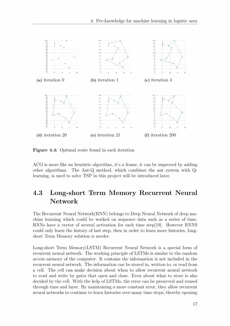
ACO is inspired by the behavior of that ants selecting paths when they search food.The paths selection that ants made are depending on the pheromones generated byprevious ants. The stronger the pheromones are, the higher probability is. Hence,ants communicate in this method to find the best way to their food. According tothis feature, although the algorithm may start with making many wrong selections,it will converge to the optimal one after several iterations. An instance of ACO onTSP has been shown in figure 4.4.

16


(a) iteration 0 (b) iteration 1 (c) iteration 4

(d) iteration 20 (e) iteration 21 (f) iteration 200

Figure 4.4: Optimal route found in each iteration

ACO is more like an heuristic algorithm, it’s a frame, it can be improved by addingother algorithms. The Ant-Q method, which combines the ant system with Q-learning, is used to solve TSP in this project will be introduced later.

4.3 Long-short Term Memory Recurrent NeuralNetwork

The Recurrent Neural Network(RNN) belongs to Deep Neural Network of deep ma-chine learning which could be worked on sequence data such as a series of time.RNNs have a vector of several activation for each time step[19]. However RNNScould only learn the history of last step, then in order to learn more histories, long-short Term Memory solution is needer.

Long-short Term Memory(LSTM) Recurrent Neural Network is a special form ofrecurrent neural network. The working principle of LSTMs is similar to the randomaccess memory of the computer. It contains the information is not included in therecurrent neural network. The information can be stored in, written to, or read froma cell. The cell can make decision about when to allow recurrent neural networkto read and write by gates that open and close. Even about what to store is alsodecided by the cell. With the help of LSTMs, the error can be preserved and reusedthrough time and layer. By maintaining a more constant error, they allow recurrentneural networks to continue to learn histories over many time steps, thereby opening

17


a channel to link causes and effects remotely[18]. The structure of LSTM RecurrentNeural Network is shown in figure 4.5.

Figure 4.5: Structure of LSTM Recurrent Neural Network, where Xt is input andht is output.

4.4 RegressionRegression analysis method is a set of statistical processes for estimating and mod-elling the continuous variables. Regression analysis is one of supervised machinelearning methods, and is widely used for prediction and forecasting, for instance,forecasting the tendency of stock, future temperature, housing price and so on. Sinceregression analysis belongs to supervised machine learning, it has to have outputswhich normally are dependent variables Y. And corresponded independent variablesX are also needed. Besides the independent and dependent variables, there arealways unknown parameters, denoted as β, which may represent as a scalar or avector. So a regression model relates Y to a function of X and β normally representsas[12]:

Y ≈ f(X, β)The approximation is usually formalized as:

E(Y |X) = f(X, β)

In order to find out the model function f, many methods have been developed,such as linear regression and regression tree. Linear regression is a most simpleand common method. A linear regression model assumes that the relationship be-tween dependent variables Y and corresponded independent variables X is linear,the model will also be added with disturbance or error.

18


Except linear regression, regression tree which could also called decision tree modelis also a widely used regression model. Differ from linear regression, regression treecan fit nonlinear characters in the data set. The main idea of regression tress is toseparate a model function into several small functions. Adding all small functionstogether, the model will be acquired. And the implementation of regression tree isshown in chapter 6.2.2.

4.5 Poisson DistributionPoisson distribution is a discrete probability distribution that express the probabilityof a given number of events occurring in a fixed interval time. The stochasticvariables fit Poisson distribution only if they are independent positive and appearrandomly. Poisson distribution is normally used to describe the probability of anumber occurs in real world, such as the number of people at bus station, the numberof consumption part in a factory. The probability function of Poisson distributionis normally described as:

P (k) = e−λλk

k!Where k is the number of occurrences and λ is the expected number of occurrenceswhich could be the average number among all k. The function is defined only atinteger values of k. Figure 4.6 is an example of Poisson distribution.

Figure 4.6: An example of Poisson distribution

Notice that the horizontal axis is the index k which is the number of temperaturein the figure, and the vertical axis is the probability of temperature k occurrencesgiven average temperature λ = 20.

19


20

5Milk run problem

Despite the Full Truckload, Volvo Cars used another logistics technique called milk-run or milk-round. Instead of letting suppliers sending their products to warehouse,Volvo decided to pick up supplies by itself. The advantage of this transportationis to maximum the load of the truck. In addition, it does not only reduce thecost of transportation expense, but also enables the delivery scheduled and efficient.In this chapter, it is presented solving a Travelling Salesman Problem(TSP) byimplementing several algorithms.Besides, because of the limitation of time and truck’s capacity, some of the supplierswon’t be visited in that tour. In the section of ’loading problem’, it is presentedhow suppliers are selected.

5.1 Loading problemThis is a process of selecting which supplier needs to be visited. It also ensures allthe supplies from selected suppliers can be loaded. The problem states like, a truckfrom X-doc will collect supplies from the suppliers after the order list, shown intable 3.2, from the X-doc is received. However, if there are too many suppliers onthat order list to travel, it is not possible for the truck to visit all of them, due tothe time and capacity limitations. In that case, some of the suppliers on that orderlist will be selected. According to the priority on the order form, supplier with highpriority will be selected to visit, if the total volume of the supplies is not exceed themaximum capacity of the truck. In order to be more efficiency, the truck shouldbe loaded as much as possible, so the proportion of truck’s inventory will also beconsidered as a factor. Supplies can’t be loaded this time will be assigned in thenext turn. One limitation of this loading problem is each supplier provide their ownspecific supplies, which means supply type is corresponding to their suppliers.

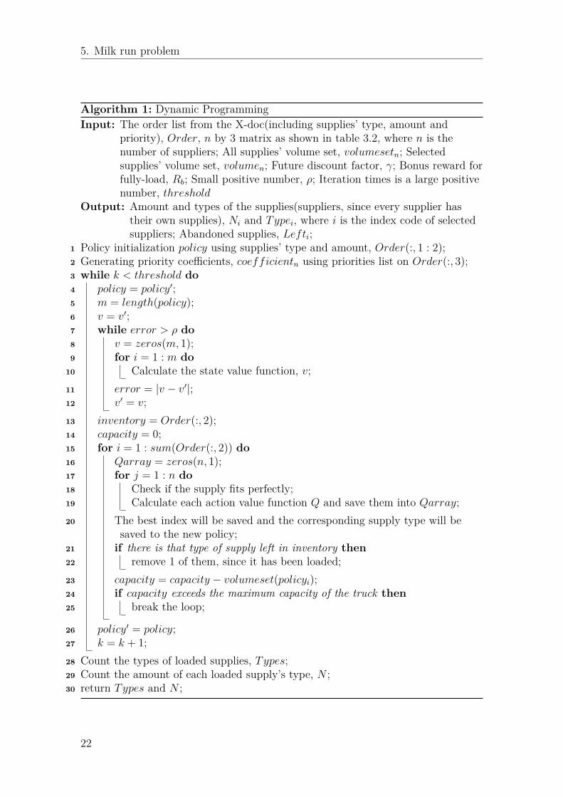
5.1.1 Dynamic Programming (DP)It is easy to implement reinforcement learning instead of other supervised learning,since the Markov Decision Process(MDP) model is easy to build in this loadingproblem, and no need to input previous data information for training process. Thepseudo-code is shown as algorithm 1.In order to form a MDP model, the first step is to find states, actions, rewards andstate value function. The states are chosen as the loading sequence of the supplies.And the actions are choices of the types of supplies. For example, an agent starts at

21

5. Milk run problem

Algorithm 1: Dynamic ProgrammingInput: The order list from the X-doc(including supplies’ type, amount and

priority), Order, n by 3 matrix as shown in table 3.2, where n is thenumber of suppliers; All supplies’ volume set, volumesetn; Selectedsupplies’ volume set, volumen; Future discount factor, γ; Bonus reward forfully-load, Rb; Small positive number, ρ; Iteration times is a large positivenumber, threshold

Output: Amount and types of the supplies(suppliers, since every supplier hastheir own supplies), Ni and Typei, where i is the index code of selectedsuppliers; Abandoned supplies, Lefti;

1 Policy initialization policy using supplies’ type and amount, Order(:, 1 : 2);2 Generating priority coefficients, coefficientn using priorities list on Order(:, 3);3 while k < threshold do4 policy = policy′;5 m = length(policy);6 v = v′;7 while error > ρ do8 v = zeros(m, 1);9 for i = 1 : m do

10 Calculate the state value function, v;11 error = |v − v′|;12 v′ = v;13 inventory = Order(:, 2);14 capacity = 0;15 for i = 1 : sum(Order(:, 2)) do16 Qarray = zeros(n, 1);17 for j = 1 : n do18 Check if the supply fits perfectly;19 Calculate each action value function Q and save them into Qarray;20 The best index will be saved and the corresponding supply type will be

saved to the new policy;21 if there is that type of supply left in inventory then22 remove 1 of them, since it has been loaded;23 capacity = capacity − volumeset(policyi);24 if capacity exceeds the maximum capacity of the truck then25 break the loop;

26 policy′ = policy;27 k = k + 1;28 Count the types of loaded supplies, Types;29 Count the amount of each loaded supply’s type, N ;30 return Types and N ;

22

5. Milk run problem

the initial state, after selecting which supply to be loaded first, the agent comes tothe second state and needs to decide which supply will be loaded next. Each actiongives a reward ’-1’. When an ’agent’ arrives that state it gains state reward, whichcan be calculated by supplies’ volume and priority. Only when the truck is fullyloaded, the action reward is zero.The state value function is the sum of action reward, following an initial policy,and product of chosen supply’s volume and priority coefficient. The initial policy isgenerated randomly corresponding to supplies’ type and amount on the order list.The limitation of truck capacity is considered, which means the truck might notload all the supplies.In the policy evaluation step, state value function will be updated using Bellmanequation shown in 5.1.

vπ(s) =∑a∈A

π(a|s)(Ras + γ

∑s′∈S

P ass′vπ(s′)) (5.1)

Where s is current state, s′ is next state, π is the policy, the discount factor isset to γ = 0.9, Ra

s is the reward at state s after taking action a, and P ass′ is state

transition probability which is the probability of taking action a at current state stransfer to the next state s′. In this case, the probability is related to the numberof left supplies’ types. More specifically, if there are three types of supplies left tobe loaded at current state, the transition probability is one third since every timethe agent can only choose one supply, to load it to the truck. As the remainingsupplies are running out, transition probability is increasing. For example, if thereis only one type left to be loaded, the agent has to choose that one, which meansthat transition probability is 100%.After assigning the rewards and actions in this equation, the state value functionwill keep updating until it is converged. The iteration stop condition is when theerror ∆, between the current and previous value function, less than a small positivenumber, which means the value function is stable and can’t be updated any more.In policy improvement step, greedy algorithm is used for proposing a new policy.The left room of the truck is calculated and applied to check whether there is anysupplies is able to fit in the left space perfectly. If there is one, a bonus reward Rb

will be added to the action value function. After the total action reward at eachstate is computed, policy will be updated by the action with the highest reward.The action value function is given by 5.2.

Qπ(s, a) = Ras + γ

∑s′∈S

P ass′vπ(s′) (5.2)

In which it is shown the action value function Q is based on the state value functionv. The new policy will then be brought back to policy evaluation to be updated.After that, another new policy will be proposed in policy improvement step. Thestop condition is a counter k larger than a pre-set positive large number. Thisiteration process is called policy iteration in order to obtain an optimal policy v∗.

5.1.2 Priority first policy proposalComparing with the dynamic programming method, this one is easier to understand.The idea is to load the supplies with high priority first. The pseudo-code is as shown

23

5. Milk run problem

in algorithm 2. This method is only considering supplies’ priority given by the order

Algorithm 2: Priority firstInput: The order list from the X-doc(including supplies’ type, amount and

priority), Order, n by 3 matrix as shown in table 3.2, where n is thenumber of suppliers; All supplies’ volume set, volumesetn; The remainingspace in the truck, storage;

Output: Loading sequence of desired supplies, policy′1 Policy initialization policy using Order;2 Split the initial policy by different types of supplies, rank1, rank2, ..., and rankn;3 for i = 1 : length(policy) do4 These sets of supply type are listed as a new policy, policy′, ordered by priority

Order(:, 3);5 storage = storage− volumeset(policy(i));6 if storage < 0 then7 policy′(i : end) = []

8 return policy′;

list from X-doc. Higher priority supplies come first, and will keep loading until thetotal volume meets truck’s maximum capacity. The remaining space, leftState, inthe truck will be watched. And if there is no room left, no more supplies can beloaded and the policy′ will also stop updating. This algorithm is simple and fast,however, the truck’s inventory might not be used efficiently.

5.1.3 Stochastic method with ’Priority first’ policy proposal’Stochastic’ means policies are proposed randomly, which is aimed for propose dif-ferent policies, as well as for avoiding the stuck in a local optimal solution, whichalways happens in heuristic optimization algorithm. It will increase the speed offinding optimal that combining priority first algorithm with stochastic method. It’spseudo code is as algorithm 3.In this loading case, desired supplies are loaded randomly to the truck until it isfull. Supplies that can’t be loaded will be saved and wait for the next truck. Thetotal rewards based on supplies’ volume and priorities will be computed. The actionwith the best reward will be saved for policy updates. However, it is an inefficientand time-consuming process if the algorithm is only based on that random method.Hence, the priority greedy method is inserted into this algorithm in order to increasethe searching speed. As it is mentioned in last section, the priority greedy is amethod which is finding an action given the highest reward on each state.

5.2 Travelling Salesman Problem(TSP)TSP has been stated in section ’ACO-TSP’ of chapter ’pre-knowledge’. In our milk-run model, the salesman who is traveling around becomes a truck from X-doc. Itneeds to travel among several specific suppliers in order to collect demanded supplies.

24

5. Milk run problem

Algorithm 3: Stochastic algorithm with Priority first methodInput: The order list from the X-doc(including supplies’ type, amount and

priority), Order, n by 3 matrix as shown in table 3.2, where n is thenumber of suppliers; All supplies’ volume set, volumesetn; Probability ofselecting priority first method, ρ; the remaining space in the truck,storage; iteration times, threshold;

Output: Loading sequence of desired supplies, policy′1 Policy initialization policy using Order;2 Split the initial policy by different types of supplies, rank1, rank2, ..., and rankn;3 Generate random parameter, p = rand;4 while iteration < threshold do5 if p < ρ then6 policy′ = policy(randperm(length(policy)));7 else8 for i = 1 : length(policy) do9 These sets of supply type are listed as a new policy, policy′, ordered

by priority, Order(:, 3);

10 for i = 1 : length(policy′) do11 storage = storage− volumeset(policy(i));12 if storage < 0 then13 policy′(i : end) = [ ];

14 Calculate the total reward, R. Find the best and save the corresponding policy′;15 iteration = iteration+ 1;

16 return policy′;

25

5. Milk run problem

The main problem is to obtain the best visiting sequence of the suppliers, whichwill be the shortest path among them. The truck starts from the X-doc and getsback to it after taken the delivery of supplies. The truck will only visit the chosensuppliers, since this is a process after the suppliers selection of loading problem. Oneassumption is made that there is only one truck can travel at a time.

5.2.1 Dynamic programmingDynamic Programming has been used again to solve another Reinforcement learningproblem on TSP. In the MDP model, it is considered the suppliers that need to bevisited are the states. And the actions are to select one of the remaining suppliers.The reward is inversely proportional to the distance between each two locationsincluding suppliers and X-doc. In state value function, the transition probabilityP ass′ depends on the number of remaining suppliers. As a reciprocal of remaining

suppliers, P ass′ will increase as the iteration goes. And it will become one in the end,

since the truck will visit each suppliers only once. The pseudo code is as shown inalgorithm 4. All the suppliers are represented as numerical order according to theA.1, for example, the X-doc is number 1. In policy initialization, the sequence ofsuppliers are generated randomly. However, the first and last one is the X-doc, sincethe truck starts from X-doc and it needs to get back to the X-doc as well after itfinishes the tour. The distance matrix is shown as A.2 and A.3, the reward matrixis their transposition with an negative sign which is used for computing the statevalue function. In policy evaluation, state value keeps updating until the error, ∆,between v and v′ is almost zero. The greedy algorithm has been implemented againin policy improvement step, in order to find the shortest path between each twolocations. In every step, action value function Q is calculated for every taken actionusing state value function v, and its value is saved to a list Qarray. The actionwith the highest Q is added to a new policy, policy′. This policy′ is brought backto policy evaluation step and generate another converged state value function. Thepolicy iteration loops a large number of times in order to find the optimal result.

5.2.2 Ant-Q in milk run problemStochastic optimization algorithm, like ant system is suitable for solving TSP prob-lem. Luca Gambardella and Marco Dorigo has proposed an algorithm called Ant-Qin 1995 [6], which combine ant system with Q-learning. Q-learning has been imple-mented to update pheromones in ant system. The pseudo code is shown as algo-rithm 5. Ant system has been introduced in ’Ant Colony Optimization(ACO)-TSP’of chapter 4, which the implementation is similar to this problem. It is consideredthe salesman is a truck, and the cities are suppliers.Starting from the Cross dock, the next state is selected by using an action choicerule according to [6] as shown in equation 5.3.

argmax{[AQ(r, u)]δ · [HE(r, u)]β}, u ∈ Jk(r) (5.3)

However, in order to be stochastic, there is a probability ρ = 1 − q0 to select thenext supplier randomly from the remaining suppliers. From the equation 5.3, it

26

5. Milk run problem

Algorithm 4: Dynamic Programming in TSPInput: List of suppliers to visit, Sn; The distance reward matrix, R; Future

discount factor, γ;Output: suppliers visit order, policy;

1 Policy initialization, policy;2 policy′ = ones(length(policy));3 while policy 6=policy’ do4 policy = policy′;5 ∆ = 1;6 while max(∆) > 10−6 do7 v′ = v;8 v = zeros(n, 1);9 leftState, which is the remaining suppliers;

10 for i = 1 : (n− 1) do11 Remove one supplier from leftState according to the policy(i);12 for j = 1 : length(leftState) do13 v(i) = v(i) + (1/length(leftState))× (R(policy(i), leftState(j)) +

γ ∗ v′(i+ 1));14 if leftState < 1 then15 break;

16 v(n) = R(policy(n), 1) + γ × v′(1);17 for i = 1 : n do18 ∆(i) = |v′(i)− v(i)|;

19 Initialize policy′;20 Reset leftState;21 for i = 1 : n− 1 do22 Qarray = zeros(m, 1);23 for j = 1 : m do24 Q(i) = R(policy′(i), leftSuppliers(j))+...gamma∗valueFunction(i+1);25 Qarray(j) = Q(i)26 BestIndex = find(Qarray == max(Qarray));27 Q(i) = Qarray(BestIndex);28 bestAction = leftState(BestIndex);29 leftState(BestIndex) = [];30 policy′(i+ 1) = bestAction;

31 return policy′;

27

5. Milk run problem

Algorithm 5: Ant-Q algorithmInput: supplies and X-doc, allstates; distance matrix, costmatrix; selecting

optimal path stability, q0; learning step, α; discount factor, γ; the relativeweight of importance of the learned AQ-values AQ and the heuristic valuesHE, δ and β; iteration times, iterationnumber; number of agents, m;

Output: Optimal visiting order of suppliers, Bestpolicy1 n = length(allstates);2 Initialization of HE = -R′, AQ = zeros(n, n), J(:, n) = allState which is the

memory matrix of remaining suppliers; the current supplier r = zeros(n+ 1,m);3 the initial supplier is X-doc, r(1, :) = 1;4 iter = 0;5 while iter < iterationnumber do6 tour = zeros(n, 2m);7 for j = 1 : m do8 Jk = J(:, j);9 for i =1:n do

10 Select the next supplier s(i, j);11 Calculate the cost between current supplier r(i, j) to every remaining

supplier;12 Save the order of them to tour(i, 2 ∗ j − 1 : 2 ∗ j) = [r(i, j), s(i, j)];13 AQarray = zeros(length(Jk), 1);14 for k = 1 : length(Jk) do15 AQarray(k) = AQ(s(i, j), Jk(k));16 AQ(r(i, j), s(i, j)) =

(1− alpha)× AQ(r(i, j), s(i, j)) + α× γ ∗ ×max(AQarray);17 r(i+ 1, j) = s(i, j);

18 for k = 1 : m do19 for i = 1 : size(tour, 1) do20 L(k) = L(k) + costmatrix(tour(i, 2 ∗ k − 1), tour(i, 2 ∗ k));

21 ∆AQ = W/min(L);22 Update AQ value using ∆AQ,

AQ(r, s)←− (1−α) ·AQ(r, s) +α · (∆AQ(r, s) +γ ·Max(AQ(s, z))), z ∈ Jk(s);23 Save the best visit order and save it to Bestpolicy;24 iter = iter + 1;25 return Bestpolicy;

28

5. Milk run problem

is found the selection depending on two matrix AQ and HE. HE here is the costmatrix, and AQ is the Ant-Q value keeps updating during the iteration. The updateequation of AQ is shown on line 22 in algorithm 5.

29

5. Milk run problem

30

6Management in factories

In this chapter, the theory and knowledge introduced in chapter 4 are implemented.The implementation of the algorithms will be used to solve specific problem in VolvoCars. The implementation tools are introduced in section 6.1. Then the predictionproblem is shown in section 6.2 and the optimization the storage can be found insection 6.3.

6.1 Implementation toolsThere are many programming language could be chosen for machine learning, butsince Python has more useful libraries, such as Scikit-learn, Keras, SciPy, all ofthem were used in this thesis work. So the programming language Python waschosen. Spyder in Anaconda was chosen as integrated development environmentfor programming because it is a open source cross-platform integrated developmentenvironment for scientific programming in the Python language. What is more,visible consoles and variable explorer, excellent debugging function is also the goodreason for choosing Spyder. In addition, in order to build neural network and makesure algorithms could work, Tensorflow is added in python environment. Excepttensorflow, several machine learning libraries such as Panda, Numpy, Keras, Scikit-learn and SciPy are also used to simplify the programming work.

6.2 The prediction of demand and consumptionAccording to the table 3.1, the information about consumption and call off datafrom PLUS system of Volvo cars is about date and quantities of each part. So theprediction problem is defined as a time series problem. And the most popular so-lution for time series prediction problem is using regression analysis methods andRecurrent Neural Network with Long Short Term Memory (LSTM). In this section,the implementations of regression analysis methods and Recurrent Neural Networkare presented base on the data provided by PLUS system.

6.2.1 Recurrent Neural NetworkIn this section, Recurrent Neural Network is introduced and implemented in Pythonusing the Keras machine learning library to address a demonstration time-series pre-

31

6. Management in factories

diction problem.

The most important process in solving time series prediction problem by LSTM Re-current Neural Network is to build features for input data as training set to fit themodel. The solution is to look back of previous information, which is the numberof previous time steps to use as input variables to predict the next time period. Forexample, if the value of look back is 5, which means the quantities of part for 5days before will all become features for current date. The Algorithm 6 presents thecomplete persuade code for creating features for training sets.

Algorithm 6: Building features for data setInput: dataset, look backOutput: featureX, labelY

1 featureX = [ ];2 labelY = [ ];3 for i in range (length of dataset - look back -1) do4 temporary value = dataset[i:(i+look back),0];5 featureX.append(temporary value);6 labelY.append(dataset[i+look back,0]);7 return featureX, labelY

After building features for the data, it is necessary to split data into train and testdata sets. The train data sets is used to fit model, and test data sets is to test themodel to check how the model fit new unseen data. The Algorithm 7 presents thecomplete persuade code for splitting data sets into test and train sets.

Algorithm 7: Splitting data set into test and train setInput: dataset, train size, look backOutput: TrainX, TrainY, TestX, TestY

1 Train set = dataset[0:train size, :];2 Test set = dataset[train size:, :];3 TrainX, TrainY = create feature(Train set, look back);4 TestX, TestY = create feature(Test set, look back);5 TrainX = np.reshape(TrainX, (TrainX.shape[0], 1, TrainX.shape[1]));6 TestX = np.reshape(TestX, (TestX.shape[0], 1, TestX.shape[1]));7 return TrainX, TrainY, TestX, TestY

Notice that the create feature in Algorithm 7 is function of the Algorithm 6.

The data sets for training the model is done, LSTM network is ready to be designedand fitted for the problem. It’s simple to build a LSTM Recurrent Neural Networkwith the help of Keras library. The Algorithm 8 presents the complete persuade codefor building LSTMmodel, fitting the data sets and predicting the future information.

32


Algorithm 8: Train model and predict dataInput: TrainX, TrainY, TestX, TestYOutput: Model

1 model = Sequential();2 model.add(LSTM(64, input shape=(1, look back)));3 model.add(Dense(32));4 model.add(Dense(16));5 model.add(Dense(8));6 model.add(Dense(1));7 model.compile(loss=’mean squared error’, optimizer=’adam’);8 model.fit(trainx, trainy, epochs=500, batch size=1, verbose=2);9 trainPredict = model.predict(trainx);

10 testPredict = model.predict(testx);11 trainPredict = scaler.inverse transform(trainPredict);12 trainy = scaler.inverse transform([trainy]);13 testPredict = scaler.inverse transform(testPredict);14 testy = scaler.inverse transform([testy]);

Notice that since LSTM are sensitive to the scale of the input data, the data setsare normalized using the MinMaxScarler preprocessing class from the Scikit-learnlibrary. So the predictions should do inverse normalize to revert back to quantityunit.

6.2.2 Regression

In this section, regression analysis methods are introduced and implemented inPython using the SciKit-learn machine learning library to address a demonstra-tion time-series prediction problem.

Similar to the create feature function of Algorithm 6 for LSTM Recurrent NeuralNetwork (RNN), features of data sets are also needed for training regression mod-els. The same idea as using look back method for building features for RNN, it iscalled shift feature for regression analysis. However, differ from look back method,regression analysis shift all the data at the same time. As an example in table 6.1,lag 1 means move all data one grid down and lag 4 means move all data four griddown. If there is no data, it will replace by Not a Number (NaN). And when lagstart from 2 and end at 4, the features for 2019/3/25 will be [720, 1080, 1080].The benefit for using lag start and lag end than look back method is the createdfeatures are more feasible.

33


Time Quantity Lag 1 Lag 2 ... Lag 42019/3/19 1080 NaN NaN ... NaN2019/3/20 1080 1080 NaN ... NaN2019/3/21 720 1080 1080 ... NaN2019/3/22 2520 720 1080 ... 10802019/3/25 1080 2520 720 ... 1080

... ... ... ... ... ...

Table 6.1: An example for time shifting features

Except shift features for regression method, there is also time features for regressionmethod. The time features could be weekday, holiday and season. For instant, whenthe date is 2019/3/19, the feature ’Tuesday’ could be added. Algorithm 9 presentsthe complete code for building time and shift features.

Algorithm 9: Building features for data setInput: dataset, lag start, lag end, target encodingOutput: featureX, labelY

1 last date = data["timestamp"].max();2 dataset.set index("timestamp",drop = True, inplace = True);3 for i in range (lag start, lag end) do4 dataset["lag[ ]".format(i)] = dataset.y.shift(i);5 dataset["month"] = dataset.index.month;6 dataset["weekday"] = dataset.index.weekday;7 dataset["weekend"] = dataset.weekday.isin([5, 6]) * 1;8 dataset["quarter"] = dataset.index.quarter;9 if target encoding then

10 dataset["weekday avg"] = calculate the average quantities of all weekday;11 dataset["month avg"] = calculate the average quantities in the same month;12 dataset["weekend avg"] = calculate the average quantities of all weekend;13 dataset["quarter avg"] = calculate the average quantities in the same quarter;14 dataset = dataset.drop(["month","weekday", "weekend","quarter"], axis = 1);15 laberlY = dataset.dropna().y;16 featureX = dataset.dropna().drop("y", axis=1);17 return featureX, labelY;

Notice that if target encoding is true, the time features will be replaced the averagequantities of corresponded feature.

There is one more function needed, which is predict function. The predict functionis to build features for future date. So with the help of future features, future in-formation could be predicted by fitted model. Algorithm 10 presents the completecode for building features for future date.

34


Algorithm 10: Predict future informationInput: model, predictX, lag start, lag end, predictYOutput: PredictY

1 predictY[0:lag start] = model.predict(scaler.transform(predictX[0:lag start]));2 for i in range(lag start, length(predictX)) do3 lastline = predictX.iloc[i-1];4 index = predictX.index[i];5 predictX.at[index, "lag".format(lag start)] = predictY[i-1];6 for j in range(lag start + 1, lag end) do7 predictX.at[index, "lag[ ]".format(j)] = lastline["lag[ ]".format(j-1)];8 predictY[i] = model.predict(scaler.transform([predictX.iloc[i]]))[0];9 return predictYFinally, it is able to use created features to fit the model, and then using fitted modelto predict future information by using prediction function. The regression model iseasy to be called by using SciKit-learn library. Algorithm 11 presents the completecode for fitting regression models and predicting future information.

Algorithm 11: Train model and predict dataInput: TrainX, TrainY, TestX, TestYOutput: Model

1 scaler = StandardScaler();2 x train scaled = scaler.fit transform(x train);3 x test scaled = scaler.transform(x test);4 lr = GradientBoostingRegressor(n estimators=100);5 lr.fit(x train scaled, y train);6 yfuture = predict future(lr, scaler, xpred, ypred, lag start, lag end);7 yfit = lr.predict(np.concatenate((x train scaled, x test scaled)));Notice that the regression model showed in Algorithm 11 is only Gradient BoostingRegressor, but there are more regressors could be called by SciKit-learn library, suchas Linear Regressor, Adamtree Regressor, and etc.

6.3 Optimizing storage in factoriesIn this section, the solution for optimizing the quantity of parts in factories is pre-sented. At last the pseudo code for the algorithm is also presented.

This optimization problem is derived from Jacks’ car rental problem which hasdescribed in section 4.1.2. Two parking lots took place by two factories of VolvoCars, at the mean time the transportation goods will be the consumed parts infactories. The rental and return cars are replaced by Consumption parts in factoriesand corresponded Call-off parts from suppliers. In Jacks’ car rental problem, thenumber of cars will be transferred between each parking lots to satisfy the rentalrequirements of each lot for maximum returns. How ever in this problem, there is no

35


transit between each factory, instead the X-doc will supply factories for insufficientparts because of the parts from Call-off will normally less than consumption infactories. But if storing too many parts in factories and transferring too many partscould cost too much money, so the problem will be to find the best quantities ofparts should store in factories and the best quantities should be transferred fromX-doc to factories, and finally the result will have maximum returns.

6.3.1 InitializationThere are some parameters need to be defined for particular problem. Table 6.2shows the parameters are used in the algorithm.

1 Number of Factory2 Max storage in Factory3 Max move parts4 Capacity in X-doc5 Discount rate6 Factory profit7 Supplier cost6 X-doc cost

Table 6.2: Parameters for optimizing storage in factories

Since the number of states are related with the quantity of each part could be storedin the factories, states can be defined with help of Max storage in factory in table6.2. The same to the initial policy, initial state value and action can be defined withMax move parts and number of factory in table 6.2. The algorithm 12 presents thedefinition of policy, state values and actions.

Algorithm 12: Algorithm define action, policy and state valueInput: Number of Factory, Max storage in Factory, Max move partsOutput: State value, Policy, Actions

1 Policy = np.zeros((Number of Factory, Max storage in Factory + 1));2 State value = np.zeros((Number of Factory, Max storage in Factory + 1));3 Actions = np.arrange(0, Max move parts + 1);Notice that the max range of Actions should be increased by 1, because in np.arrange,the end of interval is not included. The Policy and State value should include thestate when there is no part left in factory, so the range of Policy and State valuealso add one more.

6.3.2 Expected ReturnThe expected return actually is the result of Bellman equation which can also besummarized as the probability of being in some subsequent state given a particulateaction, multiplied by the reward for being in this position plus the discounted valueof being some subsequent state. The state here is related with the quantities of

36


consumed and replenished parts. And the total rewards includes the profit fromfactory and also should minus the cost from suppliers and X-doc. Since the problemuses dynamic programming as a solution, the bellman equation is used to updatestate value function. So the expected return will update the state value function, italso can help to find best policy.

In order to find the maximum returns, it’s necessary to look through all the states,then add all the values of every states together to get total return. So two loops areneeded for look through all the possibility of both consumption and replenishmentin the factory. Since the probability of being in some quantities of parts is different,a model for probability distribution is needed. And for the quantities of parts isan independent, positive and stochastic number in real life, Poisson Distributionfits the probability model in this problem perfectly. The detailed introduction ofPoisson Distribution is described in section 4.6. Then the total probability shouldmultiply the probability of number of parts of consumption and replenishment. Thealgorithm 13 presents the completed persuade code of expected return.

Algorithm 13: Expected returnInput: Number of part in factory, Number of transported part, state valueOutput: Returns

1 Returns -= X-doc cost * Number of transported part;2 for consumption in factory from Poisson lower bound to Poisson upper bound do3 Number of parts in factory = min(Initial number of part in factory, number of

transported part);4 Real Consumption in factory = min(Number of parts in factory, Consumption

in factory);5 reward = Real Consumption in factory * Factory profit;6 Number of parts in factory -= Number of parts in factory - Real Consumption

in factory;7 for replenishment in factory from Poisson lower bound to Poisson upper bound

do8 Current Number of parts in factory = min(Number of parts in factory +

replenishment in factory, Max storage in factory);9 Returns -= replenishment in factory * Supplier cost;

10 Probability = Poisson(consumption in factory, Predicted consumption infactory) * Poisson(replenishment in factory, Predicted replenishment infactory);

11 returns += Probability * (reward + Discount rate * state value[CurrentNumber of parts in factory]);

Notice that the reason for states are only looked through from Poisson lower boundto Poisson upper bound is if the number of state is not in the range of Poisson bound,the probability will be zero. So the number of quantities for both consumption andreplenishment outside the Poisson bound is not necessary to be concerned. What ismore, the Poisson function is called from SciPy libraries. The first variable as inputfor Poisson function is the variable waited to calculate probability. The second input

37


is the average number of the variable, so in this case, the value is the predicted dataof consumption or replenishment in factories.

6.3.3 Policy IterationPolicy in this problem is the quantities of each part moving from X-doc to factories.So the problem now becomes to find best policy in order to maximize returns. Sincedynamic programming is used, policy and state value will be updated step by steptogether with Bellman equation in Expected returns. The process of updating policyand state value is called policy iteration. Policy iteration can be separated into twoparts depends on updating the policy or state value, which is policy evaluation andpolicy improvement. Policy iteration will keep running until there is no change inpolicy.

6.3.3.1 Policy Evaluation

Policy evaluation is the process for updating the state value according to currentpolicy. State value is calculated by algorithm 13 Expected return. Since the policyof every state need to be updated, the for loop is needed to look through all thestates in two factories. In this problem states are the number of quantities of part infactory. Policy evaluation will keep running until the change of state value less than1× 10−4. The algorithm 14 presents complete persuade code of policy evaluation.

Algorithm 14: Algorithm for evaluating policyInput: Number of factory, Max storage in factory, state value, policyOutput: New state value

1 for State value change > 1 ∗ 10−4 do2 New state value = np.copy(state value);3 for j in range of Number of factory do4 for i in range of Max storage in factory + 1 do5 New state value = Expected return(i, policy[j,i], New state value[j, :]);

6 State value change = np.abs((New state value - state value)).sum();7 State value = New state value;

6.3.3.2 Policy Improvement

After finishing the process of policy evaluation, the new state value is ready forupdating policy. Policy improvement is the act of looking at all actions could takefrom a given state, acting greedily by choosing the action that gives the highestreturn with respect to new state value. Then the action which gives the highestreturn will be replace old action in the policy. In this problem, actions are the allpossible number of quantities of parts moving from X-doc to factories, and the initialactions are all zero for the corresponded states. The algorithm 15 presents completepersuade code of policy improvement.

38


Algorithm 15: Algorithm for improving policyInput: Number of factory, Max storage in factory, State value, Policy, ActionsOutput: New policy

1 for policy change 6= 0 do2 New policy = np.copy(Policy);3 for j in range of Number of factory do4 for i in range of Max storage in factory + 1 do5 action returns = [ ];6 for action in range of Actions do7 action returns.append(Expected return(i, action, State value[j, :]));8 New policy = Actions[j,np.argmax(action returns)];

9 Policy change = (New policy 6= Policy).sum();10 Policy = New policy;

39


40

7Results

This section states the valid results of the solutions of the loading and TSP problemin milk-run, also the demand prediction and storage optimization of managementin factories, which can be found in chapter 5 and 6 respectively.

7.1 Management in factories

There are mainly two important aspects to check the quality of machine learningalgorithms, which are time and accuracy. The results of two problems will be dis-cussed more under these two aspects. Section 7.1.1 presents the results of predictionproblem and results of optimization of storage in factories are introduced.

Normally, machine learning is used to deal with huge number of data, so running timeis an important fact. Besides, the running time also depends on the performanceof computer. The algorithms implemented in this thesis work were tested on anDell XPS 15 laptop with specification shown in Table 7.1. The other aspect isthe accuracy, especially for prediction problem. So mean square error was used topresent the error between predicted data and original data.

Component SpecificationProcessor i7-7700HQ, up to 2.8[GHz]RAM 8[GB],2400[HZ]GPU GTX1050 4[GB]

Hard Drive NVMe 250[GB] SSD

Table 7.1: Specifications of computer

The requirements and consumption data of 11 parts from 11 corresponded suppli-ers are selected for presenting the algorithms more specifically and the performanceof algorithms more intuitively. All 11 parts will be firstly predicted for future in-formation by forecasting algorithms and then be optimized their best quantities infactories to achieve maximum profit for factories. In table 7.2 presents the suppliers’code and parts number of selected 11 parts.

41

7. Results

Supplier Part number0347A 31694057A426K 32130197AD9P4 31386348AD883 31699307AEA3C 31377912AEGFW 31690924AEHPD 31658471BA7ZA 31362330CK06U 31386236D0RYB 31349975DXQLA 31455915

Table 7.2: Suppliers and corresponded parts

Notice that the name and location of suppliers’ code are mentioned in Table 7.6 insection 7.2.1.

7.1.1 The prediction of demand and consumption

In this section, the results of Recurrent Neural Networks algorithm and regressionanalysis algorithms are presented and compared. The first step is to compare theresults between Recurrent Neural Networks and all Regressors. Then the best algo-rithm will be used for prediction based on real data.

The data of part 31353931 randomly selected from PLUS system is used for compar-ing all algorithms. Figure 7.1 shows the quantity tendency of part 3135391, wherethe horizontal axis is the Call-off date of part, and vertical axis is the amount ofpart for Call-off. The implementation of regression method and Recurrent NeuralNetwork will both use this data for comparison. Running time and mean absoluteerror were used to judge the performance of algorithms.

42

7. Results

Figure 7.1: An example of presented data of consumption

Firstly, linear regression was used. Linear regression needs fitted data has linearfeature, but from figure 7.1, the data set does not show any linear feature, so theresult is quite bad. The mean absolute error for train set is 45%, and test set has15.54 % mean absolute error. What is more, the running time of linear regressionwas 0.298 seconds. The result of linear regression is presented in figure 7.2.

Figure 7.2: Prediction by Linear regression

The next is Random Forest regression. Random Forest regression is able to fitnonlinear data so the result is much better than linear regression. For RandomForest regression, the mean absolute error for train set is 15.56%, and test set has4.86 % mean absolute error. What is more, it costed 0.382 seconds to finish runningthe code. The result of Random Forest regression is presented in figure 7.3.

43

7. Results

Figure 7.3: Prediction by Random Forest regression

What is more, Gradient Boost Regression Tree is also used for prediction. GradientBoost Regression Tree is similar to Random Forest regression, both of them can fitnonlinear data set. The mean absolute error for train set is only 7.14%, and testset has 3.70 % mean absolute error. The running time is still a little shorter thanRandom Forest which is only 0.346 seconds, so Gradient Boost Regression Tressis better than Random Forest regression. The result of Gradient Boost RegressionTree is presented in figure 7.4.

Figure 7.4: Prediction by Gradient Boost Regression Tress

Finally, LSTM Recurrent Neural Networks was implemented for predicting testingdata. LSTM Recurrent Neural Networks belongs to supervised learnign which isdifferent with regression analysis algorithms. But in this problem, the performance

44

7. Results

of LSTM Recurrent Neural Networks is not good. The mean absolute error for trainset is 30.06%, and test set has 9.50 % mean absolute error. The mean error fortest set is not higher, this is because the model is over fitting. From figure 7.5, itcan be easily seen that there is lag for test sets compared with original data. Thereason for this situation is the model directly use current value as prediction datawhich is also caused by over fitting. Except accuracy, the running time was also notsatisfied. It took 198.98s to finish running complete algorithm which is much longerthan regression analysis algorithms.

Figure 7.5: Prediction by LSTM Recurrent Neural Networks

All in all, Gradient Boost Regression Trees is selected for predicting selected 11parts of 11 different suppliers. The figure 7.6 and figure 7.7 shows the result of onepart 31377912 from supplier AEA3C as an example. The rest results are shown inAppendix.

45

7. Results

Figure 7.6: An example of prediction for the call-off of part 31377912

Figure 7.7: An example of prediction for the call-off of part 31377912

The algorithm also predicted the next 3 days’ consumption and requirements in thefactory which is listed in the table 7.3. The rest predicted results of the rest 10 partsare also listed in the Appendix.

Future date Predicted Call-off Predicted requirements Inventory2020/3/27 8:00 260.12 303.65 1642020/3/27 8:00 251.38 301.482020/3/27 8:00 251.68 309.61

Table 7.3: An example of prediction result

46

7. Results

The results will keep using for optimization problem as an example for the nextsection 7.1.2, and the value of results will round up to the closest multiple.

7.1.2 Optimization of storage in factoriesAccording to the predicted data in table 7.3, parameters are specific defined in thisparticular problem. Volvo Cars has two factories and a X-doc, one is in Torslandaand the other is in Ghent, the X-doc locate at Czech. One of suppliers for ’Full TruckLoad’ (FTL) is also locate in east Europe. Base on the distance between supplierand X-doc to two factories, the cost for transporting from suppliers to factories is 5credits and the transportation from X-doc to factories will cost 3 credits. Since theconsumed parts are used for assembling cars, it should be concerned as profits forthe factories, and defined as 10 credits.

Discount rate γ is also an important parameters in Markov Decision Process whichpresents value of future rewards. When γ close to zero, it leads to "myopic" evalu-ation. And when γ close to one, it leads to "far-sighted" evaluation. The discountrate in this problem was defined as 0.9, because the future best rewards could effectcurrent returns were wanted. In this case, the result can be converged to the bestrewards much faster.

What is more, based on the data predicted by regression and Recurrent NeuralNetwork method, the quantities of eleven parts are arrange from two digits to fourdigits. Since states mean can present how many parts are left in factories and thenumber of state based on the maximum storage of parts in factories, during thetest, the maximum storage was set to 700, there will be 701 states altogether. Therunning time for 701 states was 6.5 hours which was unworthy. So if the quantities ofparts are larger than 1000, the quantities would be counted every 100 parts. In thisway, the states will reduce to 11 states. Doing the same process to the quantities ofparts larger than 100, but the quantities would be counted every 10 parts. Finally,the states, maximum storage in factories, maximum moving parts from X-doc tosupplier can be united in two digits. The maximum storage of parts in factories are90 unit and maximum moving parts are 20 unit. For example, 20 unit for quantitiesof moving parts larger than 100 means the maximum moving parts is 200 parts, forquantities of parts larger than 1000 means the maximum moving parts are 2000.With this operation, the running time can be reduced to 0.5 hours, but still bereasonable and accurate.

Parameters ValueMax storage in Factory 90/900/9000

Max move parts 20/200/2000Discount rate 0.9Factory profit 10Supplier cost 5X-doc cost 3

Table 7.4: The values set for parameters in maximum storage in factories problem

47

7. Results

After the parameters for code were defined, the results were finally get. The totaltime for running the code is 5000s which is quite satisfied. One of 11 parts 31377912are selected as as an example. The parts are from supplier AEA3C. The table 7.5presents the optimal policy for parts 31377912. The left column of the table is thenumber of parts in factory which is also the states for dynamic programming. Theright column is the number of parts should be transported from X-doc to the factorywhich is also the actions in dynamic programming. For example, the table showsthat if there are only 10 parts left in the factory, 200 parts should be transportedsince the maximum transported parts is 200. And it is easy to find that when thereare 390 parts left in the factory, no parts need to be transported, so the best quan-tity of part 31377912 should be stored in the factory is 390, which could achievemaximum rewards for the factory.

Noticed that the rest results of 10 parts from 10 suppliers are listed in Appendix.With all the results for transporting, the order will be listed for the Milk-run prob-lem.

Number of parts left in factory Number of parts need to be transited from X-doc0 20010 200... ...190 200200 190... ...380 10390 0400 0... ...900 0

Table 7.5: An example of result of storage optimization problem

7.2 Milk-run

The results of this section will be divided in two parts. The first one is the typeand amount of the supplies that need to be collected, which can represent whichsuppliers need to be visited. The other is the optimal visiting sequence of the chosensuppliers. The best path can be found easily with the help of Google Maps.

7.2.1 Selected Suppliers

According to the order form from the X-doc, shown as table 7.6, the result of loadingproblem has been computed using both reinforcement learning, stochastic methodand priority greedy method.

48

7. Results

order Supplier Quantity Priority12 Hanon System Autopal(0347A) 200 114 Continental Automotive Czech Republic(A426K) 500 84 Benteler SK Automotive Ltd(AD9P4) 1300 913 MAHLE Behr Mnichovo Hradiste(AD883) 200 35 YanFeng Slovakia Automotive Interior Systems(AEA3C) 200 610 Brose Prievidaza, spol. Ltd(AEGFW) 700 1011 BWI Czech Repblic(AEHPD) 20 48 Cooper-standard Automotive Ceska republika(BA7ZA) 190 715 Benteler automotive rumburk s.r.o(CK06U) 200 23 WITTE NejDeck(D0RYB) 2000 112 Autoneum CZ(DXQLA) 90 5

Table 7.6: An example of order form

In stochastic method combine with priority greedy, the selected suppliers and amountof supplies need to be collected are shown as table 7.7. From the output of our MAT-LAB code, it is found supplier 2, 5, 11, 12, 13 and 15 are selected to be visit andsupplier 14, 4, 10, 8 and 3 are abandoned due to the limitations. The truck’s capac-ity is set to 5.0005 units here. Where the 0.0005 is volume of the smallest supplies.The purpose of adding that is to figure out if the algorithm is able to fill the freespace of the truck with small size supplies. The probability of proposing priorityfirst policy is set to 0.2 and the iteration time is 100 to make sure the generation ofdifferent kinds of policy combinations and the priority first proposal has been active.The code runtime is about 2.8.

Table 7.7: Results of Stochastic with priority greedy method in loading problem

supplier order amount of supplies visit or not12 200 X14 0 ×4 0 ×13 200 X5 110 X10 0 ×11 20 X8 0 ×15 200 X3 0 ×2 90 X

The result of reinforcement learning method has been listed in the table 7.8. As itis shown, supplier 2, 5, 11, 12, 13, 14 and 15 has been selected. The discount factorγ has been set to γ = 0.9 here. Maximum capacity of the truck is 5.0005 units. Andthe bonus discount for fully loading is 0.3. Iteration time is set to 100 as the one instochastic method in order to do the comparison.

49

7. Results

Table 7.8: Result of reinforcement learning in loading problem

supplier order amount of supplies visit or not12 200 X14 1 ×4 0 ×13 200 X5 110 X10 0 ×11 20 X8 0 ×15 200 X3 0 ×2 90 X

7.2.2 Optimal pathSince the suppliers has been selected, the optimal path among them will be generatedusing Ant-Q, reinforcement learning and stochastic method.The result of Ant-Q is shown in a visit sequence of suppliers. After that, bringthem into the Google Maps and obtain the overview of the optimal route. Usingthe selected supplier list from stochastic method, which is supplier 2, 5, 11, 12, 13and 15. Bring them into our Ant system, we obtain the optimal visit sequence(innumerical order): 1, 11, 15, 13, 2, 14, 12, 5 and 1, where 1 is the X-doc. The optimalroute overview is shown as figure 7.8. The total path length is 1383km according toit. The runtime of Ant-Q in MATLAB is about 0.1 second.

Figure 7.8: Optimal route of Ant-Q algorithm

In ant-Q, the number of agents has been set to 7, which is the amount sum of

50

7. Results

suppliers and the X-doc. The learning step α = 0.1, optimal path stability q0 is0.9, two weight factors δ = 1 and β = 2, the parameter W , that used to calculatethe ∆AQ, is 10. Iteration number has been set to 300 to make sure that the Ant-Qobtain the best result.According to the reinforcement learning method, the sequence is: 1, 13, 15, 2, 12,14, 5, 11 and 1. The route in Google Maps is shown as figure 7.9. The discountfactor is γ = 0.9.

Figure 7.9: Optimal route of Reinforcement learning

As it is shown, the total path length here is 1444km. RL took 11.899 seconds to getthe best result when the iteration number is set to 300, as the same as the one inAnt-Q learning. However, RL do not need many iterations, it converged very fast.The best result can be obtained within 0.048 second.

51

7. Results

52

8Discussion and future work

This chapter discussed the differences among the methods used for solving X-docwarehousing and milk-run problems. Pros and cons of AI and ML have been dis-cussed compared with traditional optimization methods.

8.1 Management in factoriesAs results shown in section 7.1, the outcome of algorithms for two problems satisfythe expectations, but there are still some insufficient area need to be improved. Soin this section, the results of algorithms will be analyzed firstly, and then futurework will be discussed.

8.1.1 Prediction methodIn prediction problem for warehouse management, the purpose was to use a timeseries data set to predict the output value for future date. Normally, the outputis just a numerical variable like quantity, temperature, population and so on, sothe difficulty for time series prediction problem is to build features as input to findconnection between the output. In a word, the performance of predicted result ishighly depending on the data sets.

In this thesis work, the information in data sets that can be used is only a series ofdate and the corresponded value of quantities of parts in factories. So the featuresbuilt for fitting models are only previous quantities of parts, and regression analysismethods can fit simple, periodic numerical variable perfectly, this is the reason whyregression analysis algorithms are much better than LSTM Recurrent Neural Net-works. However if the data set has large concussion or does not show any periodicfeature, the prediction with regression analysis will occur errors. Especially whenthe test set has different tendency with training set, it will occur very large error.

However, compared with regression analysis methods in this thesis project, the re-sults of LSTM Recurrent Neural Networks are worse. The reason for this situationstill might because the simple data sets with single feature. From figure 7.5, itcould be easy to find that the predicted amounts of test set is lag than the originalamounts, which means the predicted amounts are over relying on the amounts oneday before, that equal to the previous day. The solution for the lag is to add morefeatures in the feature, for instance, the colour of interior according to the seasons.

53

8. Discussion and future work

The gender of customers could also be a feature for training. In one word, addingmore features could increase the accuracy of the model. Differing from regressionanalysis methods, LSTM Recurrent Neural Network can recognize not only the nu-merical variable as features but also the characteristic like gender, colour, commentsfor cutomers and so on. Then in the future, the results of LSTM Recurrent NeuralNetwork could be much better and more accuracy.

8.1.2 Optimization methodIn optimization problem, the solution for finding the best amounts of parts shouldstored in the factories is to solve Markov decision process as model by dynamicprogramming based on reinforcement learning. The results of this solution is goodenough, but as normal problem for reinforcement learning is that the time for run-ning code is quite long when there are huge states and actions. There are a fewmethods for reducing the running time in the future. Firstly, the initial value forthe actions were set to all zero in this thesis project, this could increase steps for it-eration process. So the initial value for the actions could be changed to the amountsof parts related with the predicted value which might closer to the best value forthe actions. What is more, except the dynamic programming to solve Markov deci-sion process, there are still some more solutions for dynamic programming such asMonte-Carlo methods, Temporal-Difference Learning methods, and so on. All thesemethods can be tried to reduce the running time of code and compare accuracybetween each other in the future.

8.2 Milk-run ProblemFrom the result in the last chapter, it was found that both optimization methodand machine learning method can both solve the loading and Travelling Salesmanproblems. In this section, the differences between them were analyzed.

8.2.1 Loading problemIn loading problem, the aim was to select suppliers which is most wanted. Themethod depended on the amount, volume of supplies and the maximum capacity ofthe truck which was used to transport. As shown in table 7.7 and table 7.8, it isfound that the reinforcement learning method can use small supplies to fill the freespace in the truck while the stochastic method can not. In reinforcement learningmethod, there was a bonus, which was activated when the truck is loaded withoutany free space. Once the bonus was active, the reward was remembered in state valuefunction which was able to have effect on the next iteration. That was a learningprocess. However, the bonus point was not considered in stochastic method, becausethe policy was generated randomly every time instead of depending on previousfactors. Due to the priority first and random proposed policy, supplies were loadedtype by type, until the truck can’t load any more. After all, the reinforcementlearning method made the truck more efficiency. If the ρ, which weigh the relative

54


probability of random proposed policy and priority greedy policy, was very large,it needed time to make lots of attempts on the different combinations of policies.While ρ was small, the order of suppliers was mainly based on the priority from theorder form.Instead of adjusting manually, reinforcement learning made the machine learneditself, which was the advantage of machine learning in this problem. The futurework will be that more suppliers will be considered in this loading problem. Otheroptimization methods can be implemented in this problem and to see if they canobtain a better result.

8.2.2 Traveling Salesman ProblemAfter selecting suppliers, the next task is to optimize the route among them. Ac-cording to the results in the last chapter, both RL and Ant-Q algorithm were ableto generate optimal visiting sequence among the selected suppliers. As it is shownin the 7.8 and 7.9, Ant-Q learning approach gave a better result than the rein-forcement learning, since this is the first attempt of implementing RL in TSP, asAnt-Q has been studied before. However, as it is mentioned before, RL methoddidn’t need many iterations to get the optimal result. This is because in the step ofpolicy improvement of RL, the action value function, Q, which is just to computethe total distance among the selected suppliers. It is proved that there is potentialto implement RL to solve this kind of problems and functions, like value functions,can be improved for a better result.

55


56

9Conclusion

The work of this thesis project has covered implementation and discussion of theAI and ML in field of logistics. Forecasting and optimizing problems of a supplychain system have been modeled, and solved with different optimization methodsand ML approaches. The results proved that it is possible to implemented AI andmachine learning in the field of logistics. It has been shown that the potential of im-plementing reinforcement learning in loading problem, travelling salesman problemand warehouse optimization. The implementation of supervised learning in inven-tory prediction of factories. Thesis work also resulted in comparison of stochasticmethod and machine learning on optimization problem.

Especially for the time prediction problem. Time series forecasting problem are adifficult type of predictive modeling problem. It is already a popular research di-rection in economy, warehouse management, weather forecasting, and so on. In thisthesis project, a regression analysis method which belongs to supervised learningapproach was chosen because the data sets for learning are simple and only timeseries sets with corresponded value of parts’ amount. However, forecasting by deepneural network is still at a very beginning phase, it should have a huge prospect inthe future.

In a conclusion that this thesis project proved that AI and machine learning couldbe a good tool for solving problems in logistic, so it is necessary to have more futurework to dig deeper in this area. It could bring a lot of profits for the company.

57

9. Conclusion

58

Bibliography

[1] "Predicting Logistics Delivery Demand with Deep Neural Networks", Yao-sanLin, Yaofeng Zhang, I-Ching Lin, Che-Jung Chang, International Conferenceon Industrial Technology and Management, 2018

[2] "Can Deep Reinforcement Learning Improve Inventory Management? Per-formance and Implementation of Dual Sourcing-Mode Problems", Joren Gijs-brechts, Robert N. Boute, Jan A. Van Mieghem, Dennis J. Zhang, KU Leuven,Northwestern University, Washington University in St. Louis, December 17,2018

[3] "Reinforcement Learning for Solving the Vehicle Routing Problem", Moham-madreza Nazari, Afshin Oroojlooy, Martin Takac, Lawrence, Lehigh University,21 May, 2018

[4] "Vehicle Routing Problem: Simultaneous Deliveries and Pickups with SplitLoads and Time Windows", Yong Wang, Xiaolei Ma, Yunteng Lao, YinhaiWang, Haijun Mao, University of Washington, 1st November, 2012

[5] "Mastering the game of Go with deep neural networks and tree search", GoogleDeepMind, 2016

[6] “Ant-Q: A Reinforcement Learning approach to the traveling salesman prob-lem”, Luca M. Gambardella, Marco Dorigo, Proceedings of the Twelfth Inter-national Conference on Machine Learning, Tahoe City, California, July 9–12,1995

[7] “Logistics management and strategy competing through the supply chain, fifthedition”, Alan Harrison, Remko van hoek, Heather Skipworth, Pearson Educa-tion Limited 2002, Saffron house 6-10, Kirby street, London, 2014

[8] "Reinforcement Learning: An Introduction", Richard S.Sutton, AndrewG.Barto, Second edition, The MIT Press, Cambridge, England, 2018

[9] "Comparison of ARIMA and Random Forest time series models for predictionof avian influenza H5N1 outbreaks", Michael J Kane, Natalie Price, MatthewScotch, Peter Rabinowitz, BMC Bioinformatics 15, 2014

[10] "Simplified Modeling and Solving of Logistics Optimization Problems", HannoFriedrich, Jonathan Gumpp, Technical university of Darmstadt, 2014

[11] "Classification and Regression by Random Forest", Andy Liaw, MatthewWiener, R News, 2012, [http://CRAN.R-project.org/doc/Rnews/]

[12] "Forecasting functions for time series and linear models", Rob J. Hyndman,George Athanasopoulos, Christoph Bergmeir, Gabriel Caceres, Leanne Chhay,Mitchell O’Hara-Wild, Fotios Petropoulos, Slava Razbash, Earo Wang, FarahYasmeen, R package, April 2018

59

Bibliography

[13] "Comparison of stochastic and machine learning methods for multi-step aheadforecasting of hydrological processes", Georgia Papacharalampous, HristosTyralis, Demetris Koutsoyiannis, Stochastic Environmental Research and RiskAssessment, 2019

[14] "Supply chain inventory optimisation with multiple objectives: an industrialcase study", Lionel Amodeo, Haoxun Chen, Aboubacar El Hadji, university oftechnology of Troyes, France, 2008

[15] "Stochastic local search procedures for the probabilistic two-day vehicle routingproblem", Karl F.Doerner, Walter J.Gutjahr, Richard F.Hartl and GuglielmoLulli, university of Vienna, University of Milano Bicocca, Austria, 2008

[16] "Artifical intelligence in logistics", DHL Custuomer Solutions & Innovation,Represented by Matthias Heutger, DHL CSI, Germany, 2018

[17] "Solving strategic and tactical optimisation problems in city logistics", PaoloGianessi, University of Paris 13 Nord, Paris, 2014

[18] "Long Short-Term Memory Recurrent Neural Network Architectures for LargeScale Acoustic Modeling", Hasim Sak, Andrew Senior, Francoise Beaufays,Google, USA, 2014

[19] "An Empirical Exploration of Recurrent Network Architectures", Rafal Joze-fowicz, Wojciech Zaremba, Ilya Sutskever, Google, USA, 2015

60

AAppendix 1

A.1 Tables

Table A.1: Suppliers list

X-doc: P3 Logistic Park 1Autoneum CZ(DXQLA) 2

WITTE NejDeck(D0RYB) 3Benteler SK Automotive Ltd(AD9P4) 4

YanFeng Slovakia Automotive Interior Systems(AEA3C) 5Hella Slovakia Signal - Lighting(AD0UM) 6

Volvo Car Corporation Engine Skovde(C7CUL) 7Cooper-standard Automotive Ceska republika(BA7ZA) 8

Promens, Inc (AEJFK) 9Brose Prievidaza, spol. Ltd(AEGFW) 10

BWI Czech Republic(AEHPD) 11Hanon System Autopal(0347A) 12

MAHLE Behr Mnichovo Hradiste(AD883) 13Continental Automotive Czech Republic(A426K) 14

Benteler automotive rumburk s.r.o.(CK06U) 15Rochling Automotive Koprivnice S.r.(AECQX) 16

I

A. Appendix 1

Table A.2: Shortest Distance among suppliers corresponding to the suppliercode(units: km) part 1

X-doc DXQLA D0RYB AD9P4 AEA3C AD0UM C7CUL BA7ZAX-doc 0 141 161 308 342 343 1195 146DXQLA 138 0 299 212 246 236 1285 75.9D0RYB 162 304 0 444 478 478 1163 303AD9P4 308 212 442 0 39 125 1487 166AEA3C 343 246 477 38.2 0 123 1523 202AD0UM 344 246 478 125 121 0 1446 202C7CUL 1195 1331 1160 1488 1523 1447 0 1348BA7ZA 146 76.1 303 167 201 202 1348 0AEJFK 315 178 449 132 180 68.1 1392 174AEGFW 406 309 540 177 165 66.3 1428 264AEHPD 185 328 46.4 467 502 502 1191 327AB6RA 355 175 489 224 222 105 1332 213AD883 54.4 124 215 325 359 359 1210 160A426K 378 199 512 254 242 111 1332 237CK06U 120 193 190 388 464 422 1081 223AECQX 320 189 503 244 283 115 1330 205

Table A.3: Shortest Distance among suppliers corresponding to the suppliercode(units: km) part 2

AEJFK AEGFW AEHPD AB6RA AD883 A426K CK06U AECQXX-doc 312 404 184 354 56.9 329 123 325DXQLA 170 298 322 175 128 195 198 191D0RYB 450 540 46.5 490 217 509 182 505AD9P4 132 176 465 224 321 206 388 246AEA3C 170 181 501 270 357 230 465 280AD0UM 68.1 65.7 501 105 357 112 423 115C7CUL 1397 1431 1189 1332 1203 1333 1077 1331BA7ZA 173 263 326 191 157 210 223 199AEJFK 0 120 472 61.2 329 71.3 395 69.2AEGFW 120 0 563 155 419 144 485 154AEHPD 473 564 0 513 241 533 226 529AB6RA 62.1 155 512 0 296 21.2 485 15.5AD883 294 421 243 292 0 311 71.9 307A426K 71.4 144 535 21.2 320 0 485 10.8CK06U 363 484 224 361 69.2 487 0 376AECQX 75 153 526 15.6 310 10.9 380 0

II

AI & ML in warehousing and milk-run

Documents

Transcript of AI & ML in warehousing and milk-run