1

Ahmed Abed1, Nick Thom1, and Luis Neves1

1Nottingham Transportation Engineering Centre, the University of Nottingham, Nottingham, UK.

Corresponding author: Ahmed Abed

Email address: ahmed.abed@nottingham.ac.uk

Nick Thom

nicholas.thom@nottingham.ac.uk

Luis Neves

Luis.Neves@nottingham.ac.uk

Abstract

Variability of pavement design parameters has always been a concern to pavement designers

and highway agencies. A robust pavement design should take into account the variability of

the design inputs and its impact on the reliability of the design. In this study, the variability

effect of thickness and stiffness of pavement layers was investigated. The variability of these

parameters was described by their mean values, standard deviations and probability

distribution functions. Monte Carlo Simulation method was utilised to incorporate variability

of the design parameters and to construct the probability distribution function of the outputs.

KENLAYER software was used to calculate pavement response at predetermined critical

locations; pavement reponse was then used to predict pavement performance regarding

permanent deformation, bottom-up and top-down fatigue cracking by using the mechanistic

empirical pavement design guide (MEPDG) models. A Matlab code was developed to run that

analysis and obtain the probability distribution function of pavement performance indicators

over time. It was found that the variability of pavement layer thickness and stiffness has a

significant impact on pavement performance. Also, it was found that not only the mean of the

predicted performance indicators is increasing over time, but the variance of these indicators is

also increasing. This means that pavement condition cannot be described by the mean values

of the indicators but by the probability distribution function which can describe pavement

condition at any reliability level.

2

Introduction

The concept of incorporating variability of pavement design variables in pavement analysis and

design was first introduced by Darter and Hudson (1973). They stated that due to the stochastic

nature of pavement design parameters, a probabilistic design approach that takes into account the

inherent variability and uncertainty of those parameters must be implemented in order to improve

the reliability of the pavement design process. They also developed a design model that calculates

the reliability of the design as the probability that the number of load application that the pavement

can sustain is larger than the expected number of load application. Despite that their work was

limited to the effect of variability of pavement design parameters on pavement serviceability loss

due to traffic loading, it can be considered as the basis for the probabilistic pavement design

because it became possible for pavement engineers to design the pavement based on a certain level

of reliability. Later, the reliability principle was included as a part of AASHTO (1986) and

AASHTO (1993) design guides; it was defined as the degree of certainty that a pavement designer

adds to assure that the designed pavement maintains a certain level of serviceability over the design

period. Such as ESALR=ESAL50%+SE×ZR where ESAL50% is the predicted number of load

application at 50% reliability, SE is the standard error, ZR is the standard normal deviate, and

ESALR is the predicted number of load application based on the desired reliability level. Therefore,

a reliability factor that can be selected based on the road type was developed which merely meant to

assure that the designed Equivalent Single Axle Load (ESAL) exceeds the expected ESAL.

In a similar reliability analysis approach, the Mechanistic-Empirical Pavement Design Guide

(MEPDG) (NCHRP, 2004a) included the effect of variability of pavement design parameters on the

design process; but this time the variability was considered by its impact on the predicted pavement

distresses rather than the expected ESAL. The variability effect was evaluated by calculating the

standard error between the predicted distresses via MEPDG models and the observed distress from

3

real pavement sections, and calibration factors were suggested to minimise the perdition error. The

benefit of this approach is that pavement designers can evaluate the variability impact on every

pavement distress, which can be quite useful in understanding the sensitivity of the distress against

the variability of the design inputs. Hence identifying the critical design parameters to design

against certain dominant distress types.

Generally, pavement performance prediction can be either deterministic or probabilistic (Amador-

Jiménez and Mrawira, 2011; Wang, Zaniewski, & Way, 1994). The deterministic prediction can be

divided into three models, mechanistic, empirical, or mechanistic-empirical (M-E). A detailed

discussion regarding these models can be found elsewhere (K. A. Abaza, 2004; Collop and Cebon,

1995; George, Rajagopal, & Lim, 1989). The main drawback with these models is the incapability

of these models to address input dispersions thus only the mean value of the studied indicator is

obtained after the analysis (Valle, 2015). Furthermore, to improve the reliability of the deterministic

methods, the designers apply safety factors based on engineering judgment which may result in

either “overdesign” or “underdesign” problems (Huang, 2004). On the other hand, the probabilistic

prediction requires previous knowledge of the design input distributions to obtain a distribution

rather than a definite value of the analysed indicator. This approach has been suggested to include

uncertainty associated with the design inputs to improve design reliability (K. A. Abaza, 2014; Butt,

Shahin, Feighan, & Carpenter, 1987; Hassan, Lin, & Thananjeyan, 2015; Li, Haas, & Xie, 1996;

Wang, et al., 1994). Most of these studies, however, have implemented Markov Chain to predict the

future condition of the pavement based on the previous conditions. The application of Markov chain

requires historical quality data regarding pavement condition such as assessment of distress at least

two different times in order to calculate Markov Chain transition matrix which is the central

element to predict the future state of the pavement. However, these data may not always be

available. Moreover, pavement condition prediction is performed purely based on surface distress

4

assessment. Thus the underlying mechanism that causing pavement deterioration is not included in

this analysis. In other words, pavement mechanical properties which are the main factors in

predicting the distress, are not involved in the prediction process. Furthermore, using the same

transition matrix to predict pavement future condition may not be realistic since pavement

deterioration rate may not be constant. Accordingly, some researchers suggested using a non-

homogeneous Markov Chain to address this issue (K. Abaza and Murad, 2007; K. A. Abaza, 2015).

In contrast, a different transition matrix has to be used to predict future pavement condition for

every period of performance. However, at the end of every analysis period, the transition matrix has

to be calibrated based on the difference between the predicted and the actual pavement condition.

One of the interesting techniques in risk analysis studies is Monte Carlo (MC) simulation method.

The concept of this method is to probabilistically predict the performance of a system by randomly

generating a set of inputs according to their probability distribution functions, then using analytical

models that link the inputs with the outputs to predict the system behaviour; running the model for

many simulations results in several predictions of the system performance, the predictions can then

be used to establish the probability distribution of the output (Ayyub and Klir, 2006). In pavement

engineering applications, Xiao (2012) applied MC method to analysing and improving the

reliability of the MEPDG model. He developed a probabilistic design tool that was able to evaluate

the reliability of pavement design process. However, based on approximation techniques such as the

equivalent thickness and surface response methods, he developed a surrogate model to predict

pavement response and smoothness. This means that pavement stress and strain were calculated

based on an approximate solution rather than the exact solution of the multilayer elastic system

which may affect the accuracy of the simulation process. Wu, Yang, & Sun (2017) applied MC

filtration method to run a sensitivity analysis to the MEPDG. They demonstrated that this method

could be a valuable tool to identify the significant pavement design parameters, they also observed

5

that 350 simulations were required to rank the critical and important parameters. The simulation

time, however, was relatively high, it took about fifty hours to simulate fifteen years five hundred

times.

Despite the approach that is implemented to address the reliability of pavement design, we have to

consider that there is significant variability in pavement design parameters that have to be taken into

account in the design process. Table 1 (Valle, 2015) presents a summary of the variability

associated with the design primary input parameters expressed by the Coefficient of Variations

(CoV) and the probability distribution function of those parameters. This table provides an obvious

idea of the level of variability exists in the thickness and stiffness of pavement layers which are the

main pavement design input parameters. The thickness of the bituminous layers can vary 7-10%,

whereas it can vary 12-15% for the granular layers, whereas the stiffness can vary 10-20% for the

bituminous layers and 10-30% for the unbound pavement layers. This level of variability can

significantly affect the accuracy and reliability of the predicted pavement performance.

Accordingly, this study aims to develop a probabilistic performance prediction tool that considers

the variability of the design parameters in the prediction process by the application of MC method.

6

Table 1. Pavement layer thickness and stiffness variations and their suggested probability

distributions (Valle, 2015)

Property Description

Range

CoV %

Typical

CoV%

Type of

distribution

Reference

Lay

er t

hic

kn

ess

Bituminous

surface

3-12 7 Normal

Timm et al. (2000),

Noureldin et al. (1994)

3.2-18.4 7.2 Normal Aguiar-Moya et al. (2009)

Bituminous binder

course

11.7-16 13.8 Normal Aguiar-Moya et al. (2009)

5-15 10 Normal Noureldin et al. (1994)

Granular base

10-15 12 Normal Noureldin et al. (1994)

6-17.2 10.3 Normal Noureldin et al. (1994)

Granular subbase 10-20 15 Normal Noureldin et al. (1994)

Ela

stic

modulu

s

Bituminous layers

10-20 15 Normal Noureldin et al. (1994)

10-40 Lognormal Timm et al. (2000)

Granular base

10-30 20 Normal Noureldin et al. (1994)

5-60 Lognormal Timm et al. (2000)

Granular subbase

10-30 20 Normal Noureldin et al. (1994)

5-60 Lognormal Timm et al. (2000)

Granular subgrade

10-30 20 Normal Noureldin et al. (1994)

20-45 Lognormal Timm et al. (2000)

Model Development

The model developed in this study is graphically represented in Figure 1. Firstly, the model

generates random design variables based on their mean values and their probability distribution

functions. Secondly, it sends the generated values to Kenlayer software to calculate pavement

7

response (strains) at predefined critical locations. Finally, it uses M-E models to predict pavement

distress, which were: bottom-up fatigue cracking, top-down fatigue cracking, and permanent

deformation. The critical strains considered in this study were: the horizontal tensile strain at the

bottom of the base layer to predict bottom-up fatigue cracking, the horizontal tensile strain at the

pavement surface to predict top-down fatigue cracking, and the vertical compressive strain at the

middle of each of pavement layers to predict the permanent deformation. To demonstrate the

application of the suggested model, a typical pavement structure as shown in Figure 2 has been

considered in this study. The following sections explain the details of the developed model.

Thickness of Pavement Layers

To introduce variability effect of this parameter, the recommended thickness coefficients of

variation reported in Table 1 were implemented. The thickness of pavement layers was assumed to

be normally distributed. The mean thickness values are as shown in Figure 2, whereas the standard

deviation can be calculated by multiplying the CoV by the mean values. After determining the mean

and the standard deviation of the layer thickness, random thickness values of each layer were

generated by MC method. Figure 3 presents the distributions of the generated values.

8

Figure 1. Flowchart of the simulation model

9

Figure 2. Four-layer pavement Figure 3. Thickness of pavement layers

Pavement Temperature

Pavement temperature is one of the significant inputs to calculate the dynamic modulus of the

asphaltic materials (Y. R. Kim, Underwood, Far, Jackson, & Puccinelli, 2011). To accurately

compute pavement response, it is necessary that pavement temperature at the time of the analysis be

defined so that the dynamic modulus can be calculated accordingly. Pavement temperature is

usually determined from air temperature data which can be collected from weather stations, and

several available regression models to calculate pavement temperature can be found in the

literature. The model implemented in this study is the one that was reported by Mohseni (1998) as

follows:

Temppav−low = −1.56 + 0.72 × 𝑇𝑎𝑖𝑟 − 0.004 × 𝐿𝑎𝑡2 + 6.26 log10(𝐻 + 25) Equation 1

Temppav−high = 54.32 + 0.78 × 𝑇𝑎𝑖𝑟 − 0.0025 × 𝐿𝑎𝑡2 − 15.14 log10(𝐻 + 25) Equation 2

where Temppav−low is the low pavement temperature °C, Temppav−high is the high pavement

temperature, 𝑇𝑎𝑖𝑟 air temperature °C, 𝐿𝑎𝑡 is the latitude of the section degrees, and 𝐻 is the depth to

10

pavement surface mm. These models result in two pavement temperatures; one is lower, and one is

higher than the air temperature. If the air temperature is rising, then the pavement is absorbing

energy and pavement temperature is lower than the air temperature; if the air temperature is

dropping, then the pavement is emitting energy and the pavement temperature is higher than the air

temperature. Accordingly, for the same air temperature there are different possible pavement

temperatures, one is lower, one is higher than the air temperature, and the third one is an average of

the low and high pavement temperatures.

Furthermore, these models require only air temperature data and the latitude of the analysed section

to calculate pavement temperature. However, to calculate the air temperature at any time, it is

necessary to model the air temperature as a function of time. Since the air temperature periodically

changes over time, then it is logical to assume that the air temperature can be modelled as a sine

wave of time. To prove this assumption, local weather data of Nottingham city for the past forty

years was downloaded from UK Forecast (2019) website and implemented in this study. The

average monthly temperature was then predicted using the following trigonometric function:

Temptime = AMT +MaxT−MinT

2× sin(2π ×

𝑇𝑚

12+ θ) Equation 3

where Temptime is the predicted temperature as a function of time, AMT is the average monthly

temperature, MaxT is the maximum temperature, MinT is the minimum temperature, 𝑇𝑚 is the

time in months, and θ is a shit angle to fit the sine wave with temperature data. The optimisation

function “SOLVER” embedded in Excel software was used to calculate model parameters; a

sample of the real data and the predicted air temperatures and pavement temperatures as well are

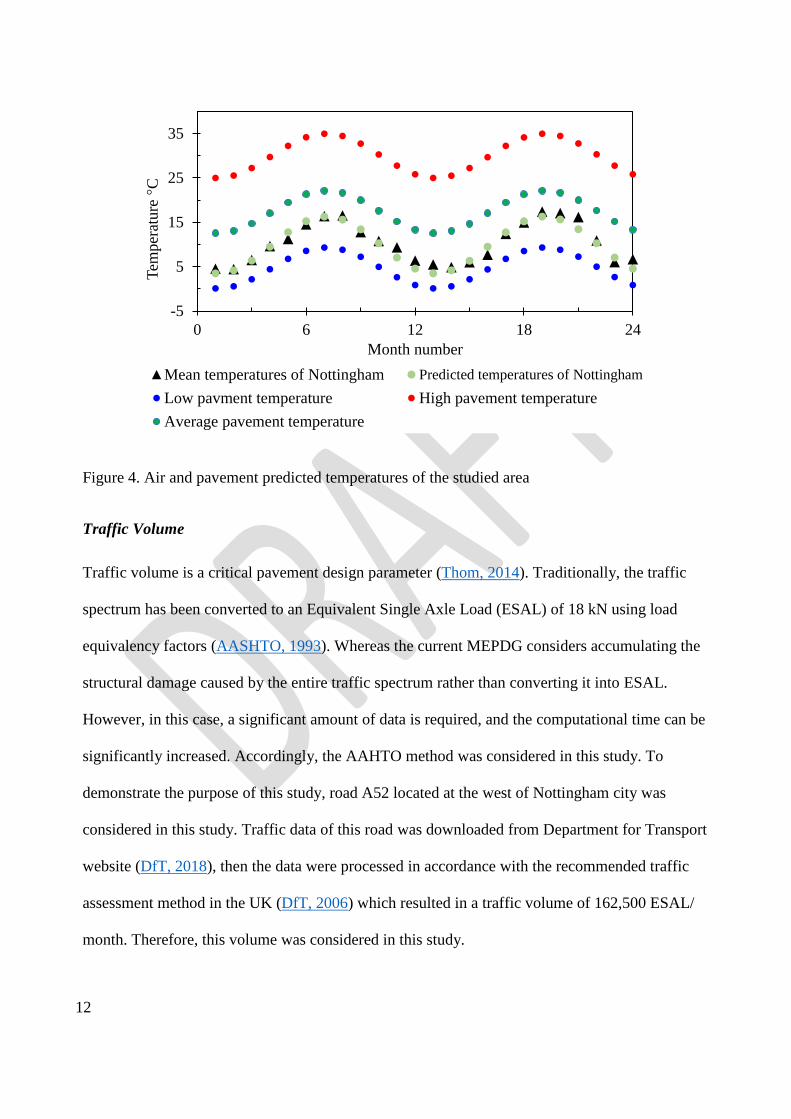
presented in Figure 4. This figure shows that the predicted average monthly temperature fits very

well with the measured average monthly temperatures. It also shows that monthly air

11

temperatures can result in three pavement temperatures; low and high pavement temperatures that

are calculated based on Equation 1 and Equation 2, and an average of these temperatures. The

low pavement temperature represents pavement temperatures at night and early morning times;

the high pavement temperature represents pavement temperatures at the noon and afternoon

times; whereas the average pavement temperature represents pavement temperatures between

early morning and noon times. Based on this assumption, the entire spectrum of pavement

temperatures can be represented, and the pavement damage at each of these temperatures can be

predicted and accumulated in the analysis. Traffic volume of every month was then divided into

three parts, 10% at the low pavement temperature, 70% at average pavement temperature, and

20% at the high pavement temperature. This assumption may approximately match traffic hourly

distribution with temperature hourly distribution, but it is necessary to account for pavement

damage that is accumulated at different temperatures and traffic volumes. Furthermore, this

procedure should improve the damage prediction process because the damage in this case is

calculated based on traffic damage and pavement temperatures when the traffic is passing.

Certainly, pavement temperatures can be divided more finely and different traffic volumes can be

assigned to each part, but this can be a time-consuming process.

12

Figure 4. Air and pavement predicted temperatures of the studied area

Traffic Volume

Traffic volume is a critical pavement design parameter (Thom, 2014). Traditionally, the traffic

spectrum has been converted to an Equivalent Single Axle Load (ESAL) of 18 kN using load

equivalency factors (AASHTO, 1993). Whereas the current MEPDG considers accumulating the

structural damage caused by the entire traffic spectrum rather than converting it into ESAL.

However, in this case, a significant amount of data is required, and the computational time can be

significantly increased. Accordingly, the AAHTO method was considered in this study. To

demonstrate the purpose of this study, road A52 located at the west of Nottingham city was

considered in this study. Traffic data of this road was downloaded from Department for Transport

website (DfT, 2018), then the data were processed in accordance with the recommended traffic

assessment method in the UK (DfT, 2006) which resulted in a traffic volume of 162,500 ESAL/

month. Therefore, this volume was considered in this study.

-5

5

15

25

35

0 6 12 18 24

Tem

per

ature

°C

Month number

Mean temperatures of Nottingham Predicted temperatures of Nottingham

Low pavment temperature High pavement temperature

Average pavement temperature

13

Dynamic Modulus of the Asphaltic Layers

The dynamic modulus is one of the essential fundamental properties of asphaltic materials that is

used in the MEPDG to calculate pavement response (Y. R. Kim, et al., 2011). This property can be

directly measured by performing dynamic modulus testing. Otherwise, it can be predicted from the

mix design and binder properties. In this study, the latter method was adopted. The dynamic

modulus was predicted at different temperature and frequencies using the following model

(NCHRP, 2004b):

log 𝐸∗

= 0.00689 × [3.750063 + 0.02932 × 𝜌200 − 0.001767 × (𝜌200)2 − 0.002841 × 𝜌4

− 0.058097 × 𝑉𝑎 − 0.802208 × (𝑉𝑏𝑒𝑓𝑓

𝑉𝑏𝑒𝑓𝑓 + 𝑉𝑎)

+3.871977 − 0.0021 × 𝜌4 + 0.003958 × 𝜌38 − 0.000017 × (𝜌38)

2 + 0.005470 × 𝜌34

1 + 𝑒(−0.603313−0.313351×log(𝑓)−0.393532×log(𝜂))]

Equation 4

where E* is dynamic modulus MPa, η bitumen viscosity 106 Poise, f loading frequency Hz, Va air

void content %, Vbeff effective bitumen content %, ρ38 cumulative retained on the sieve 19 mm, ρ34

cumulative retained on the sieve 9.5mm, ρ4 cumulative retained on the No. 4 sieve, and ρ200 is

cumulative retained on the No. 200 sieve. After determining the dynamic modulus at different

temperatures and frequencies, a master curve was constructed by the application of the time-

temperature superposition principle; then the following generalised logistic function was fitted to

the test data since this function was reported to give a proper fitting (M. Kim, Mohammad, &

Elseifi, 2015):

14

log(|E∗|) = δ +α

(1 + λ × eβ+γ×log fr)^(1λ) Equation 5

where |E*| is the dynamic modulus, δ is the minimum value of the complex modulus, α is the

difference between the minimum and maximum values of the dynamic modulus, and λ, β, and γ are

shape parameters. Further details regarding the application of the time-temperature superposition

principle and the construction of dynamic modulus master curves can be found elsewhere (Airey,

1997; M. Kim, et al., 2015). The developed master curves for the surface and base layers based on

this model are presented in Figure 5. This figure indicates that the base layer has a higher dynamic

modulus than the surface layer. This is because a binder grade of 15-25 dmm has been considered

for the base layer, and a binder grade of 40-60 dmm has been considered for the surface layer in

accordance with British standard BS EN 13108-1 (BSI, 2006).

However, the derived dynamic modulus master curves of the surface and base layers do not take

into account the variability associated with this parameter. Because so far, the modulus is calculated

as a function of temperature and frequency. But Table 1 indicates that the coefficient of variation of

the bituminous layers is 10-20%, which means that the variability associated with this parameter

has not yet included in the analysis because the dynamic modulus calculated by equations 3 or 4 is a

deterministic value at a specific temperature and frequency. To overcome this issue and to include

the variability of the dynamic modulus in the simulation, the calculated modulus at every

temperature and frequency was assumed to be the mean value at these conditions, and the standard

deviation was calculated accordingly. Then the dynamic modulus that includes the variability was

calculated using the following equation:

15

𝐸(𝑇,𝑓)𝑣𝑎𝑟∗ = 𝐸(𝑇,𝑓)𝑑𝑒𝑡𝑒𝑟

∗ × (1 +𝐶𝑜𝑉

100× 𝑅𝐺𝑉) Equation 6

where 𝐸(𝑇,𝑓)𝑣𝑎𝑟∗ is the dynamic modulus at a certain temperature and frequency that is randomly

generated based on its level of variability, 𝐸(𝑇,𝑓)𝑑𝑒𝑡𝑒𝑟∗ is the deterministic dynamic modulus

determined from the master curves, CoV the coefficient of variance, and RGV is a randomly

generated value from the standard Gaussian distribution (mean= 0 and standard deviation=1).

Basically, this equation adds the variability associated with the dynamic modulus to the

deterministic dynamic modulus calculated from the master curves. Figure 6 shows the dynamic

modulus of the surface layer that was developed based on the prescribed method. It can be seen that

the modulus varies significantly from one case to another due to the variability associated with this

parameter.

Stiffness Modulus of the Unbound Pavement Layers

The stiffness modulus of the sub-base and sub-grade layers were calculated using the following

correlation between California Bering Ratio (CBR) and the resilient modulus (NCHRP, 2004c):

Er = 17.6142 × (CBR)0.64 Equation 7

where Er is the resilient modulus of unbound pavement layers MPa. The CBR values used in this

study were assumed to be 35% and 15% for the sub-base and sub-grade layers respectively.

Equation 7 does not take into account the variability associated with the sub-base and sub-grade

materials. Table 1 shows that the average CoV of the stiffness of these layers is 20%. By using the

recommended CoV and assuming that the calculated modulus in Equation 7 is the mean value and

by the application of the same concept of Equation 6, Figure 7 and Figure 8 were developed. The

16

figures show that the modulus of the unbound pavement layers can vary significantly, which can

have a significant impact on the prediction of pavement performance.

Figure 5. Surface and base layer dynamic modulus

master curves

Figure 6. Variations of the dynamic modulus

Figure 7. Sub-base layer stiffness modulus Figure 8. Sub-grade layer stiffness modulus

Pavement Response

Pavement performance depends to a significant extent on the way that the pavement responses to

17

the applied stress. Traditionally, pavement response has been calculated based on Burmister’s

multilayer elastic theory (Huang, 2004). There are several available programmes that can calculate

pavement response. Such as KENLAYER, JULEA, and MICHPAVE. These programmes can

calculate stresses and strains for multilayer systems. However, to run the simulation, it is required to

repeatedly calculate pavement response for thousands of times to obtain an output with a particular

distribution which may take a long time to solve one problem. To overcome this issue,

KENLAYER was utilised in a novel way to calculate pavement response; it was linked to Matlab

software as a subroutine to calculate pavement strain at predefined locations. The Matlab code

performs the following procedure to determine pavement response:

(1) It generates random input variables based on each variable’s probability distribution.

(2) It determines the average monthly air temperatures then it calculates three pavement

temperatures for each month, low and high temperatures, and the average of these.

(3) It calculates the dynamic modulus for the asphaltic layers based on the predetermined

temperatures and frequencies. Then it uses Equation 6 to add variability to the calculated

modulus based the on recommended CoV in the literature.

(4) Then it sends the generated inputs to KENLAYER programme to calculate pavement

response.

(5) Finally, it automatically extracts the analysis results (strains) from KENLAYER at

predetermined critical locations to use them in predicting pavement performance.

For bottom-up fatigue cracking, the horizontal critical tensile strain the bottom of the base layer is

used to predict the cracking damage. For the rutting, the vertical compressive strain at the middle of

each layer is used to predict this distress. For top-down fatigue cracking which initiates at pavement

surface, the horizontal tensile strain at pavement surface is in the prediction process. However, most

18

of the available pavement analysis programmes cannot accurately calculate pavement stress and

strain near the pavement surface. Huang (2004) demonstrated that KENLAYER resulted in a

difference in the calculated tensile strain at analysis depth less than 51 mm in comparison with other

software. In other words, KENLAYER was not capable of correctly calculating pavement strains at

depths less than 51 mm. JULEA software can calculate pavement response at a minimum depth of

20% of the load contact radius (Khazanovich and Wang, 2007), which means that this software may

not accurately calculate pavement response less than that depth. To overcome this issue, an

alternative method was followed, the tensile strain at the pavement surface was estimated using the

following equation (Thom, 2014):

𝜀𝑠𝑢𝑟𝑓𝑎𝑐𝑒 =𝑃

𝐸× √6 × (1 + 𝜐) Equation 8

where 𝜀𝑠𝑢𝑟𝑓𝑎𝑐𝑒 is the shear strain at the edge of the applied load, 𝑃 is traffic load, E is the stiffness

of asphalt layer, and 𝜐 is Poisson’s ratio. This equation can give a reasonable approximation to the

surface tensile strains in an easy computational effort, which makes it suitable for implementation

in pavement analysis software.

Fatigue Cracking Performance Prediction

To predict fatigue cracking performance, the MEPDG models (NCHRP, 2004c) were implemented

in this study, as follows:

FCbottom =1

60×

6000

1+e(−2c2′ +c2

′ ×log(D∗100)) Equation 9

FCtop = 10.56 ×1000

1 + e(7.0−3.5×log(D∗100))

Equation 10

19

where FCbottom is the bottom up cracking (%), FCtop is the length of top-down fatigue cracking,

c2′=-2.40874-39.748×(1+hac)^-2.856, and D is the fatigue damage of either bottom up or top down

cracking. The primary input to these models is D which was calculated in this study based on

Miner’s law (Huang, 2004) as follows:

D =∑∑ni,j

Ni,j

m

j=1

p

i=1

Equation 11

where D is the damage, p is a number of periods, m is number of load groups which equals one in

this study since only ESAL was considered in the analysis, ni,j is the predicted load applications,

and Ni,j is the allowable load application which was calculated based on the Asphalt Institute fatigue

life model, as follows (The Asphalt Institute, 1981):

FL = C × K1 × (1

E)𝐾2 × (

1

εt)𝑘3

Equation 12

where FL is the fatigue life as a number of load applications, K1, K2, andK3 are laboratory

regression coefficients, C is a fatigue life laboratory to field shift factor, E is asphalt stiffness, and εt

is the horizontal strain at the bottom (for bottom-up cracking) or surface (for top-down cracking) of

asphalt layer. To sum up, fatigue cracking can be predicted by calculating pavement response

(strains) at critical locations under specific loading and environmental conditions, using Equation

12 to calculate fatigue life, determining fatigue damage using Equation 11, then predicting the

bottom-up and top-down fatigue cracking using equations Equation 9 or Equation 10 based on the

damage location.

20

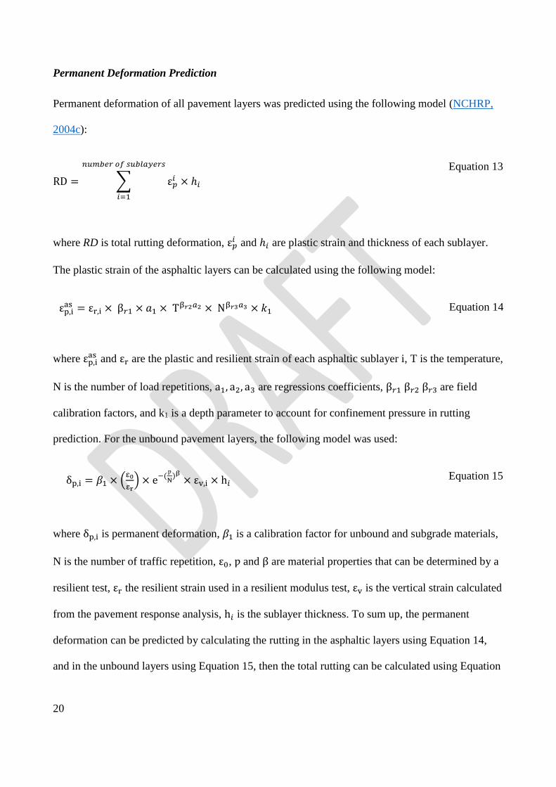
Permanent Deformation Prediction

Permanent deformation of all pavement layers was predicted using the following model (NCHRP,

2004c):

RD = ∑ ε𝑝𝑖

𝑛𝑢𝑚𝑏𝑒𝑟𝑜𝑓𝑠𝑢𝑏𝑙𝑎𝑦𝑒𝑟𝑠

𝑖=1

× ℎ𝑖

Equation 13

where RD is total rutting deformation, ε𝑝𝑖 and ℎ𝑖 are plastic strain and thickness of each sublayer.

The plastic strain of the asphaltic layers can be calculated using the following model:

εp,ias = εr,i ×β𝑟1 × 𝑎1 ×T

β𝑟2𝑎2 ×Nβ𝑟3𝑎3 × 𝑘1 Equation 14

where εp,ias and εr are the plastic and resilient strain of each asphaltic sublayer i, T is the temperature,

N is the number of load repetitions, a1, a2, a3 are regressions coefficients, β𝑟1β𝑟2β𝑟3 are field

calibration factors, and k1 is a depth parameter to account for confinement pressure in rutting

prediction. For the unbound pavement layers, the following model was used:

δp,i = 𝛽1 × (ε0

εr) × e−(

ƿ

N)β × εv,i × h𝑖 Equation 15

where δp,i is permanent deformation, 𝛽1 is a calibration factor for unbound and subgrade materials,

N is the number of traffic repetition, ε0, ƿ and β are material properties that can be determined by a

resilient test, εr the resilient strain used in a resilient modulus test, εv is the vertical strain calculated

from the pavement response analysis, h𝑖 is the sublayer thickness. To sum up, the permanent

deformation can be predicted by calculating the rutting in the asphaltic layers using Equation 14,

and in the unbound layers using Equation 15, then the total rutting can be calculated using Equation

21

13.

Results and Discussion

By applying the derived model, the performance of the studied pavement was simulated for thirty

years. To analyse the simulation results, it is critical to fit a distribution that best fits the data so that

the reliability of the system can be accurately determined. Therefore, four of the commonly used

distributions, Normal, Lognormal, Weibull, and Burr were fitted to the data as shown in Figure 9.

Then the distribution that gives the maximum log likelihood was selected, in this case, it was Burr

distribution. This distribution has a probability distribution function as follows (MathWorks®,

2015):

𝑓(𝑥|𝛼, 𝑐, 𝑘) =

𝑘 × 𝑐𝛼 × (

𝑥𝛼)

(𝑐−1)

(1 + (𝑥𝛼)

𝑐)(𝑘+1), 𝑥 > 0, 𝛼 > 0, 𝑐 > 0, 𝑘 > 0

Equation 16

where c and k are the shape parameters, 𝛼 is the scale parameter, and x is a variable. The shape and

scale parameters make this distribution flexible to fit very well different data distributions.

Accordingly, this distribution was fitted to the simulation data and utilised to calculate the

probability of the simulated stresses. Figure 10, Figure 11, and Figure 12 present the simulation

results of the bottom-up fatigue cracking (denoted by FCB_age in years), top-down fatigue cracking

(denoted by FCS_age in years), and the total permanent deformation (denoted by PD_age in years)

respectively. The results revealed that not only the means of the performance indicators are

increasing over time, but the standard deviations are also significantly increasing. This means that

the mean distress values are not useful in describing the pavement condition. The probability

distribution, however, is a reasonable way to describe the pavement condition due to its capability

of predicting the distress at any reliability level. Moreover, the results show that the pavement may

22

fail due to the top down cracking before other distress types appear. This result generally agrees

with the common structural performance of the thick pavements in the UK (Thom, Choi, & Collop,

2002).

To further implement the analysis results and to expand the application of the developed simulation

tool, the predicted measures were utilised in predicting maintenance time. The MEPDG threshold

levels (AASHTO, 2008) (bottom-up fatigue cracking <20% lane area, top-down fatigue cracking

<132.6 m/km, Rutting in HMA layers <16.5 mm) for primary highways were applied, and the

probability of an output being less than the designated threshold value was calculated from the

fitted distributions and presented against the pavement service time, as shown in Figure 13. The

results indicate that the pavement will start to exhibit severe top-down cracking between 12-15

years since during this period the probability of being less than the threshold of this distress is

dropping. The bottom-up cracking, on the other hand, will never appear even after 30 years of

service, since the percentage of the cracking at 30 years is about 2% which is much lower the

threshold value of this distress. Regarding permanent deformation, the figure shows that this

distress will appear gradually between 15-20 years and after that all simulated cases will exhibit

rutting more than 16.5mm. Accordingly, these results can be used in predicting the time to provide

maintenance by simply deciding at which probability the maintenance should be provided. For

example, if one considers a probability of 0.5 for the top-down cracking as a limit to provide

maintenance, then the analysed pavement will need maintenance after 13 years of service.

23

Figure 9. Examining different distributions to best fit simulation data

Figure 10. Predicted bottom-up fatigue cracking, % of lane area

24

Figure 11. Predicted top-down fatigue cracking, m/km

Figure 12. Predicted rutting, cm

25

Figure 13. The probability of the outputs being less than the threshold values

Number of Simulations

One last critical point to consider is the simulation time. The simulation time depends on two

factors, the simulation period and the number of simulations. The former is a user input; it is the

aim of the analysis to predict pavement performance after a specified time. Therefore, this factor

cannot be used to reduce simulation time. The latter, however, can significantly increase simulation

time if it is overestimated, and it may reduce the simulation result if it is underestimated because

increasing the number of simulations is expected to improve the efficiency of the simulation process

(Ayyub and Klir, 2006). So, this factor must be investigated in order to obtain sufficient simulation

results within a reasonable simulation time.

The effect of the number of simulations was studied by running the simulation for different times,

such as 50, 75, 100, 125, 150, 250 runs. The statistical significance of each number was then tested

against the highest number of runs assuming that this number is sufficient to construct the

probability distribution function of the outputs. A two-sample Kolmogorov-Smirnov test was

utilised to test the significance. The null hypotheses H0 of this test is that both samples are from the

26

same distribution; the alternative hypothesis H1 is that the samples are from different distributions.

Following this method, the results of all predicted distress types at a simulation period of 20 years

were tested. Interestingly, all the results were insignificantly different from the 250 case, even when

a low number of runs such as 50 simulations was considered. This means that this analysis can be

successfully performed using only 50 simulations which takes about 3.5 hours to simulate pavement

performance for twenty years.

Summary and Conclusions

Variability associated with pavement design parameters has always been a concern to pavement

designers and highway agencies. This point becomes even more critical when too many design

parameters are involved in the design process, because every parameter may add additional

uncertainty to the predicted performance. Therefore, this study aims to address this issue and

suggests a framework to probabilistically predict pavement performance and takes into account the

variability associated with the design parameters. This aim has been addressed by performing MC

simulation. The input parameters were the mean and the standard deviation of the primary

pavement design input parameters. KENLAYER was utilised in a novel way to calculate pavement

response; it was used as a subroutine with Matlab to determine pavement strains based on the

generated inputs by the code. The outputs were the probability distribution functions of the top-

down cracking, bottom-up cracking, and permanent deformation. These indicators were calculated

by implementing the MEPDG models.

The developed simulation tool was applied to simulate and predict the performance of a typical

four-layer asphalt pavement. The pavement was simulated for 30 years, the probability distribution

function of the outputs was captured every five years. The simulation results showed that the

variability of pavement design inputs has a critical effect on the simulation results. The results also

27

revealed that the probability distribution function of the outputs is expanding, and not only the mean

but also the standard deviation is increasing over time. In other words, the mean cannot successfully

describe pavement condition, but the probability distribution function which can represent

pavement status at any reliability level. Also, it was found that the Burr distribution best fits the

predicted distress types and can be used to represent the probability distribution function of these

indicators. Furthermore, tracking the probability of distress being less than threshold values over

time can be a valuable option to predict pavement maintenance time and the type of the required

maintenance. However, the question that remains open in this study is to what probability should

roads be maintained?

Limitation: Because the simulation results depend to a significant extent on the models used in the

analysis and since these models, unfortunately, were not calibrated to UK weather and material

properties, this analysis cannot yet be applied directly to UK roads. The results in the current study

are based on specific calibration factors suggested based on the experience of the authors with the

analysed pavement system and local material properties. Therefore these factors were not

mentioned in the paper to avoid misleading the readers.

Acknowledgements

The authors would like to acknowledge professor Gordon Airey and Dr Davide Lo Presti from Nottingham

Transportation Engineering Centre\ the University of Nottingham for their scientific support and valuable

comments during the development of this study.

Disclosure statement

No potential conflict of interest was reported by the authors.

References

1. AASHTO. (1986). AASHTO Guide for Design of Pavement Structures. Washington, D.C., US:

American Association of State Highway and Transportation Officials.

28

2. AASHTO. (1993). AASHTO Guide for Design of Pavement Structures. Washington, D.C., US:

American Association of State Highway and Transportation Officials.

3. AASHTO. (2008). American Association of State Highway and Transportation Officials.

Mechanistic-Empirical Pavement Design Guide: A Manual of Practice: AASHTO

Designation: MEPDG-1. Washington, DC.

4. Abaza, K., & Murad, M. (2007). Dynamic Probabilistic Approach for Long-Term Pavement

Restoration Program with Added User Cost. Transportation Research Record: Journal of

the Transportation Research Board, 1990, pp. 48-56. doi:10.3141/1990-06

5. Abaza, K. A. (2004). Deterministic Performance Prediction Model for Rehabilitation and

Management of Flexible Pavement. International Journal of Pavement Engineering, 5(2),

pp. 111-121. doi:10.1080/10298430412331286977

6. Abaza, K. A. (2014). Back-calculation of transition probabilities for Markovian-based pavement

performance prediction models. International Journal of Pavement Engineering, 17(3), pp.

253-264. doi:10.1080/10298436.2014.993185

7. Abaza, K. A. (2015). Empirical Approach for Estimating the Pavement Transition Probabilities

Used in Non-Homogenous Markov Chains. International Journal of Pavement Engineering,

18(2), pp. 128-137. doi:10.1080/10298436.2015.1039006

8. Airey, G. D. (1997). Rheological characteristics of Polymer Modified and Aged Bitumens

(Doctor of Philosophy PhD). The University of Nottingham.

9. Amador-Jiménez, L. E., & Mrawira, D. (2011). Reliability-Based Initial Pavement Performance

Deterioration Modelling. International Journal of Pavement Engineering, 12(2), pp. 177-

186. doi:10.1080/10298436.2010.535538

10. Ayyub, B. M., & Klir, G. J. (2006). Uncertainty Modeling and Analysis in Engineering and the

Sciences: Boca Raton, FL, Chapman & Hall/CRC.

11. BSI. (2006). BS EN 13108-1:2006, Bituminous Mixtures - Material Specifications - Part One:

Asphalt Concrete. The United Kingdom: British Standards Institution.

12. Butt, A., Shahin, M., Feighan, K., & Carpenter, S. (1987). Pavement Performance Predíction

Model Using the Markov Process. Transportation Research Record 1123

13. Collop, A., & Cebon, D. (1995) Modelling Whole-Life Pavement Performance. Paper presented

at the Fourth International Symposium on Heavy Vehicle Weights and Dimensions, Ann,

Arbor, USA.

14. Darter, M. I., & Hudson, W. R. (1973). Probabilistic Design Concepts Applied to Flexible

Pavement System Design CFHR 1-8-69-123-18). Center for Highway Research, The

University of Texas at Austin

15. DfT. (2006). Design Manual for Roads and Bridges, Volume 7: Traffic Assessment.

16. DfT. (2018). Traffic Counts. Retrieved Date Accessed, 2018 from

https://www.dft.gov.uk/traffic-counts/index.php.

17. George, K. P., Rajagopal, A. S., & Lim, L. K. (1989). Models for Predicting Pavement.

Transportation Research Record 1215

18. Hassan, R., Lin, O., & Thananjeyan, A. (2015). Probabilistic Modelling of Flexible Pavement

Distresses for Network Management. International Journal of Pavement Engineering, 18(3),

pp. 216-227. doi:10.1080/10298436.2015.1065989

19. Huang, Y. H. (2004). Pavement Analysis and Design United States of America: Pearson

Prentice Hall.

20. Khazanovich, L., & Wang, Q. (2007). MnLayer: High-Performance Layered Elastic Analysis

Program. Transportation Research Record: Journal of the Transportation Research

Board(2037), pp. 63-75.

29

21. Kim, M., Mohammad, L., & Elseifi, M. (2015). Effects of Various Extrapolation Techniques for

Abbreviated Dynamic Modulus Test Data on the MEPDG Rutting Predictions. Journal of

Marine Science and Technology, Vol. 23, No. 3, pp. 353-363 (2015)doi:10.6119/JMST-014-

0327-7

22. Kim, Y. R., Underwood, B., Far, M. S., Jackson, N., & Puccinelli, J. (2011). LTPP Computed

Parameter: Dynamic Modulus FHWA-HRT-10-035).

23. Li, N., Haas, R., & Xie, W.-C. (1996). Development of a New Asphalt Pavement Performance

Prediction Model. Canadian Journal of civil Engineering, 24, pp. 547–559

24. MathWorks®. (2015). User's Guide: Burr Type XII Distribution.

25. Mohseni, A. (1998). LTPP Seasonal Asphalt Concrete (AC) Pavement Temperature Models.

26. NCHRP. (2004a). Guide for Mechanistic-Empirical Design of New and Rehabilitated Pavement

Structures 1-37A).

27. NCHRP. (2004b). Guide for Mechanistic Empirical Design of New and Rehabilitated Pavement

Structures: Part 2 Chapter 2: Material Characterisation Final Report 1-37A). Washington

D.C.

28. NCHRP. (2004c). Guide for Mechanistic Empirical Design of New and Rehabilitated Pavement

Structures: Part 3 Chapter 3, Design of New and Reconstructed flexible Pavements Final

Report 1-37A). Washington D.C.

29. The Asphalt Institute. (1981). Thickness Design Manual (MS-1) (9th ed.) College Park,

Maryland.

30. Thom, N. (2014). Principles of Pavement Engineering (Second edition ed.) United Kingdom:

ICE Publishing.

31. Thom, N., Choi, Y.-K., & Collop, A. (2002) Top-down cracking, damage and hardening in

practical flexible pavement design. Paper presented at the Proc 9th International Conference

on Asphalt Pavements, Copenhagen.

32. UK Forecast. (2019). UK Weather Services. Retrieved Date Accessed, 2019 from

https://www.metoffice.gov.uk/pub/data/weather/uk/climate/stationdata/sheffielddata.txt.

33. Valle, P. D. (2015). Reliability in Pavement Design (Doctor of Philosophy. University of

Nottingham, United Kingdom.

34. Wang, K., Zaniewski, J., & Way, G. (1994). Probabilistic Behavior of Pavement. Journal of

Transportation Engineering, 120(3), pp. 358-375.

35. Wu, Z., Yang, X., & Sun, X. (2017). Application of Monte Carlo filtering method in regional

sensitivity analysis of AASHTOWare Pavement ME design. Journal of Traffic and

Transportation Engineering (English Edition), 4(2), pp. 185-197.

doi:10.1016/j.jtte.2017.03.006

36. Xiao, X. D. (2012). Risk Analysis and Reliability Improvement of Mechanistic-Empirical

Pavement Design (Doctor of Philosophy. University of Arkansas, Fayetteville.