Agricultural Subsidies in Mexico - Wilson Center · The distributive incidence of agricultural...
52
3 67 3 Agricultural Subsidies in Mexico: Who Gets What? John Scott 1 Centro de Investigación y Docencia Económicas 1 This is an abridged version of Scott (2010).
Transcript of Agricultural Subsidies in Mexico - Wilson Center · The distributive incidence of agricultural...
3
67
3
AgriculturalSubsidiesin Mexico:Who Gets What?
John Scott1
Centro de Investigación y Docencia Económicas
1 This is an abridged version of Scott (2010).


3
Agricultural Subsidies in Mexico
69
IntroductIonThis study presents a detailed and comprehensive incidence analysis of the principal agricul-tural and rural development programs (ARD) introduced in Mexico in the context of the open-ing up of agricultural markets through the North American Free Trade Agreement in 1994-2008. These programs have been the subject of various evaluations in recent years.2 The OECD and World Bank reports incorporate quantitative estimates of the incidence of agricultural subsidies at the household/producer level, as well as geographically, based on Scott (2006, 2008). The present study builds upon and extends the latter results in several respects, includ-ing an extended discussion of the relevance of distributive analysis in the evaluation of agri-cultural subsidies, a distributive analysis of the income sources and employment conditions of rural and agricultural households, an expansion in the coverage programs analyzed, and the use of more accurate measures of producer wealth to estimate the distribution of agricultural subsidies at the household/producer level.
The poverty-reduction potential of agriculture is a principal theme of the World Development Report 2008, though the report also emphasizes the growing importance of non-farm rural activities. None of the noted evaluations of agricultural policies in Mexico includes an analysis of rural/agricultural labor markets. This remains one of the least studied aspects of the rural economy in Mexico (see Esquivel 2009 for a recent research outline of this area), and has im-portant policy implications in the present context, as the regressive concentration of subsidies in the richer, northern state producers has often been rationalized by the claim that these subsidies “trickle down” to the poor through agricultural labor markets. However, given the compensatory rather than productive objectives in the design and allocation of most of these subsidies, these have tended to favor established large-scale, capital-intensive grain produc-tion, rather than the development of more labor-intensive fruit and vegetable production. There is no evidence of positive employment effects of agricultural subsidies at the state level. Over the last decade agricultural employment has declined significantly in most states, but disproportionately so in those receiving the larger subsidy shares (see section 5, below).
The study refines the benefit incidence analysis of agricultural subsidies by controlling for variations in the quality and productivity of land, as well as producer prices, at the state level, thus obtaining a better proxy of the wealth/income of beneficiaries than simple (undifferenti-ated) land holdings. This reveals that the preliminary assessments of previous studies overes-timated the degree of regressivity (concentration on wealthier producers) in the case of the delinked Procampo transfers, but underestimated the concentration in the case of Ingreso Ob-jetivo, as of most of the other subsidies concentrated on larger commercial producers. Not surprisingly, the analysis also reveals that land assets, thus adjusted, are far more unequally distributed than suggested by the unadjusted land data commonly used to measure land in-equality in Mexico and internationally (Deininger and Olinto 2002).
The study is structured as follows. Section 1 considers the relevance of distributive analysis in the present context in the light of the multiple (and often conflictive) objectives of agricul-tural subsidies. In particular, the section responds to a well-established view (among policy-makers in the sector) that dismisses such analysis as imposing equity objectives on instru-ments concerned purely with efficiency objectives. Section 2 describes and quantifies the evolution of the principal agricultural adjustment/compensatory programs in Mexico in the post-NAFTA era. Section 3 reviews the evolution of agricultural growth, productivity and em-ployment and wages, considering the possible effects of agricultural subsidies on these trends. Section 4 reviews recent data on rural poverty and human development deprivation, and ana-lyzes the income sources and labor market profile of the rural poor. Section 5 analyzes the distribution of agricultural subsidies at the state and municipal level, and its incidence on growth, productivity and employment. Section 6 presents a benefit incidence analysis of agri-cultural subsidies at the producer and household level, and estimates the (first-order) impact of ARD expenditures on rural income inequality in Mexico. Section 7 derives policy recommen-dations.
2 Recent comprehensive evaluations of agricultural and rural policies in Mexico have been produced by the OECD (2006), IADB (2007) and World Bank (2008), though only the OECD report has been published to this date (September 2009). Evaluations of Procampo have been undertaken by GEA, Auditoría Superior de la Federación (2006), and an advisory group on Procampo’s reform set up in 2008 by Sagarpa and IADB (unpublished). Alianza para el Campo has been evaluated by FAO (2005).
Subsidios para la desigualdad
70
1. Is equIty relevant? ProductIve,comPensatory and dIstrIbutIveobjectIves In agrIcultural PolIcyThe distributive incidence of agricultural subsidies in Mexico has received growing attention not only in the cited international reports, but also in a number of governmental and non-governmental initiatives, as well as in the media.3 Policy-makers within the agricultural sector, however, have traditionally been more skeptical about the relevance of equity con-siderations for the design and appraisal of agricultural policies. To motivate the distributive analysis to be presented below, it is therefore important to clarify this issue at the outset.
The design and evaluation of Mexico’s agricultural policies has often been plagued by a problem which is common in complex policy areas: the imposition of multiple, often con-flictive objectives on single policy instruments. This is often aggravated when the objec-tives are confused and implicit, rather than clearly defined. A notable example of this is the case of Procampo, as will be seen below.
At the same time, the overall conception, design and evaluation of rural development and agricultural policies has traditionally been marked by a sharp division in objectives be-tween “productive” and “social” programs, with the former concerned exclusively with in-creasing the productivity of the agricultural sector, and the latter focused on alleviating rural poverty. This division has been historically ingrained at the federal and local admin-istrations, with a strict division between the ministries responsible for “productive” pro-grams (mainly Sagarpa), and those concerned with “social” programs (mainly Sedesol). This division has been preserved in the Ley de Desarrollo Rural Sustentable and its associated budgetary instrument, the Programa Especial Concurrente para el Desarrollo Sustentable (PEC). Despite its intended function as an integrating and coordinating institutional frame-work for rural development policy, in practice the PEC has served as little more than a classification system that groups the large set of agricultural and rural development pro-grams by common functions, at the broadest level in terms of productive vs. social.
This division is consistent with a general result from modern welfare economics about the independence of efficiency from equity interventions, 4 which may be interpreted as imply-ing that “productive” programs should focus exclusively on correcting market failures to push GDP towards the economy’s productive potential (the production possibility frontier), delegating to “social” (redistributive) instruments the task of attaining a particular social optimum within this frontier. An obvious implication of this interpretation is that produc-tive instruments should be evaluated by their success in increasing productivity, not by their distributive incidence (and vice versa for social programs).
This may seem to provide a rigorous foundation for the rejection of distributive concerns in the case of agricultural subsidies. Such skepticism is of course often a thinly veiled and self-serving rationalization on behalf of established interests, 5 but it may also be a legiti-mate concern of agricultural policy-makers, especially given Mexico’s agrarian history. For example, Rosenzweig (2008) presents this concern in a recent analysis of agricultural pol-icy produced for a panel of independent experts on Procampo reform set up by Sagarpa and the IDB: “One of the reasons why agricultural policy has lost effectiveness is because of poorly-understood equity considerations… By basing transfers on the factors of production, one is necessarily seeking a productive rather than a social equity outcome. …” (pp.5-6).
Given the prevalence and basic economic logic of this claim, it is important to be as clear as possible in explaining why this is in fact an argument for considering the distributive impact of agricultural subsidies in their overall assessment, rather than ignoring it.
3 These include various forums on the reform of agricultural subsidies in Presidencia de la República, Congress (Cen-tro de Estudios para el Desarrollo Rural Sustentable y la Soberanía Alimentaria, CEDRSSA), and the excellent data base that includes Procampo and other agricultural subsidies published by FUNDAR (www.subsidiosalcampo.org.mx). The incidence of agricultural subsidies has also been reported by CONEVAL in their Informe de Evaluación de la Política de Desarrollo Social en México 2008 (graph 16. P.80), and appears to have been used in the definition of priorities in the 2010 proposed federal budget. 4 This follows from the so-called “fundamental theorems of welfare economics” which prove that every competitive market in general equilibrium is Pareto efficient, and conversely, every Pareto efficient point can be achieved through a general equilibrium (per appropriate allocation of assets).5 For example, a presentación at Sagarpa by the Asociacion Mexicana de Secretarios de Desarrollo Agropecuario (AMSDA, Sept. 2008; presented to the Secretary of Agriculture and addressed to the President of Mexico) reacting to recent reform proposals, dismissed distributive concerns as “populist”, with a sombre threat: “Unfortunately some have proposed the goal of changing PROCAMPO and Ingreso Objetivo to take away from large producers to give the small ones... It’s the Rich vs. the Poor. That sounds like demagoguery and anachronistic populism and will provoke disturbances that will undermine the stability of the country.” The presentation was delivered by Jorge Kondo, President of AMSDA, Secretary of Agriculture of Sinaloa (one of the states with the largest shares of agricultural subsidies), and apparently personally a major beneficiary of these subsidies (Merino, 2009, based on www.subsidiosalcampo.or.mx).
3
Agricultural Subsidies in Mexico
71
1 Note first that even if the conditions of the welfare theorems did apply, allowing a strict separation in the implementation of efficiency and equity policies, this would still not make the distributive effects of the efficiency instruments irrelevant. On the contrary, designing and implementing the equity instruments to achieve the social optimum would of course require precise understanding of the (collateral) distributive effects of the efficiency instru-ments. These effects could be neutral or even progressive, thus facilitating the task of the equity instruments. As we will see, agricultural subsidies in Mexico (as in most countries) are actually highly regressive, most of them even more regressive than the distribution of private incomes in the rural sector. Considering their weight in the agricultural/rural economy, this means that they are actually a significant determinant of rural inequality in Mexico. This implies that to achieve the social optimum (assuming this gives some positive weight to equity), the redistributive instruments would have to be designed to compensate for the effect of the productive instruments as well as for the other (market) determinants of inequality.
2 In fact, of course, the idealized assumptions of the welfare theorems are highly unrealistic, and especially so in the context of rural and agricultural markets and institutions. The theorems assume the existence of complete and perfectly competitive markets for all goods and factors of production, perfectly informed economic agents, and costless (perfectly in-formed) redistributive instruments. In addition to assuming no market failures, the welfare theorems assume no failures in non-market (political, government and non-government) institutions required to identify and implement a socially optimum distribution. The failure of these conditions to apply does not mean that the welfare theorems are of no practical interest, but their guiding power is “negative” or indirect rather than direct: it lies in the capacity to identify precisely and exhaustively the falsifying conditions to be addressed by public policy.
3 In the present context, this means that the efficiency and equity considerations are not eas-ily separable in the design and evaluation of agricultural subsidies and agricultural/rural development policies more generally. Given the market-failures prevalent in the rural/agri-cultural sector, large inequalities between producers in the access to inputs and markets represent a major restriction to productivity and growth. The close interdependence be-tween efficiency and equity conditions in economic growth has received much attention in recent years, as reviewed in the World Development Report 2006: Equity and Development, the WDR 2008 in the context of agriculture, and World Bank (2004, 2006) and Levy and Walton (2009) for the case of the Latin American region and Mexico, respectively. This in-terdependence may be illustrated with many specific examples, and even with the broad history of agrarian reform and agricultural support policies in Mexico over the last century. At the risk of gross simplification, this history may be summarized as follows:
a) The agrarian reform produced atomized agricultural land holdings and drastically con-strained land markets under the ejido system,
b) The principal agricultural support policies applied in this period—price-based subsidies and irrigation and other input subsidies—benefited mostly large-scale and capital (irrigation)-intensive grain producers in the North, but failed to reach the bulk of small-scale and subsistence producers created by the Reform, constraining them to low-quali-ty, low-investment, technologically primitive production units. It was only by the end of the century that a major transfer program was introduced capable of reaching the bulk of these producers (Procampo 1994), even if their share of the transfer was limited to their share in land-holdings.
c) In addition to the historical bias against small-holders, subsistence farmers and landless agricultural workers in the allocation of agricultural subsidies, poor rural households were also excluded from most social and anti-poverty programs, again until the end of the century. These were allocated with a strong urban bias which was only reversed with efforts to expand the coverage of basic education and health services to rural areas in the 1990’s, including especially the creation of the innovative Progresa CCT program in 1997 (renamed Oportunidades in 2001).
4 To recap the separation of equity and efficiency instruments: land reform and (belatedly) social programs were used to address rural inequality, while agricultural subsidies were concentrated on the larger producers on purely efficiency considerations. The outcome of these policies, as we will see bellow, is an agricultural sector which is both highly unequal and relatively inefficient, as well as resilient to reform (section 3). At the centenary of the Mexican Revolution, two decades after the “second agrarian reform”, the rural economy is still trapped in a low growth, high inequality equilibrium, barely sustaining the poorest of the poor while supporting some of the richest and most generously subsidized individuals in Mexico. This outcome reflects many failures of design and implementation within the two major policy categories (distributive and productive), but is also explained by the his-torical separation of these instruments, leading respectively (at one extreme) to a populous, commercially unviable small-holder and subsistence sector, which has survived as a form of minimal social insurance, and (at the other end) large-scale northern grain producers re-ceiving the bulk of subsidies without much evidence of significant impacts in productivity
Subsidios para la desigualdad
72
or employment (see sections 3 and 5). In the middle, are the small to middle-sized (5-20+ has) producers with undeveloped potential, constrained in their access to credit, insurance, technology, marketing and other critical inputs. These are generally not poor enough to benefit from Oportunidades or other social programs and not large enough to attract sig-nificant agricultural subsidies under present allocation criteria, but may well be the poten-tial beneficiaries with the highest impact: such support would be both more equitable and more productive, relaxing significant binding constraints on agricultural production (in contrast to large producers which are already close to their production-possibility frontiers, partly as a consequence of the cumulative effect of past historical investments in their fa-vor). A similar argument was made fifteen years ago by De Janvry et al. (1995), who showed that the strata of middle-sized producers had the most potential to benefit from support to facilitate crop reconversion and modernization under NAFTA. Unfortunately, while Pro-campo did succeed in allocating resources to these producers at least proportional to their share in cultivated land (41%, see graph 30, below), the required complementary inputs failed to reach this strata (both because the input support programs were significantly curtailed, and those which do exist are concentrated on the larger producers, see section 6, below).
2. agrIcultural trade adjustment and comPensatory Programs aFter naFtaThe principal ARD policies currently implemented in Mexico originated in the context of a broad, market-orientated reform effort to modernize the agricultural sector in the early and middle nineties, in the context of both, the opening up of agricultural commodity markets under the North American Free Trade Agreement (NAFTA) in 1994 with a 15 year transitional period, and the constitutional reform of the ejido land tenure system in 1992.
Mexico’s “second agrarian reform”, as this ambitious reform effort has rightly been labeled (by one of its principal architects, see Gordillo et al. 1999), was accompanied by extensive reforms in ARD policies, introducing more efficient (less distortionary), as well as more equitable policy instruments. The long, drawn-out “first” agrarian reform, following the Mexican Revolution, was accompanied from the Cárdenas administration in the 1930s until its formal termination in 1992, by two principal forms of agricultural support: input support (irrigation, fertilizers) and market price support (MPS). By design, these support policies where both highly distortionary and inequitable, failing to reach the small and subsistence farmers created by the agrarian reform.
Farmers were partly compensated for the gradual reduction of MPS under NAFTA through three principal support programs: a) the Programa de Apoyos a la Comercialización 6, an out-put-based subsidy program introduced in 1991, b) the Programa de Apoyos Directos al Campo (PROCAMPO), a per hectare direct transfer program decoupled from production and commer-cialization, introduced in 1994, and c) Alianza para el Campo, an investment support program (or family of programs) offering matching grants and support services, introduced in 1996. The expectation was that these programs would not only play a compensatory role in the face of growing external competition but, in the case of Procampo and Alianza, would also provide the necessary support for farmers to modernize production and switch to higher value crops in the context of the newly liberalized land and product markets.
In the context of Mexico´s dual agricultural sector and previous agricultural support policies, the decoupled design of Procampo was revolutionary in terms of efficiency as well as equity. By decoupling transfers from production/commercialization, the program was expected to minimize distortions in productive decisions and to transfer resources directly to subsistence farmers, for the first time in Mexico’s post-revolutionary history. The original decree for the creation of Procampo lists an extended list of objectives, including prominently as “one of its main objectives”, increasing the income of “2.2 million rural subsistence producers which were excluded from the support system”. 7
6 The Programa de Apoyos a la Comercialización and PROCAMPO are both managed by Apoyos y Servicios a la Comer-cialización Agraria (ASERCA).7 Decree that Regulates the Rural Direct Support Program, Procampo, DOF, July 25, 1994. The list of objectives includes (emphasis added): 1) greater participation of the rural private and social sectors to improve domestic and international competitive-ness; 2) raise the living standards of rural families; 3) modernization of the marketing system, 4) increase the capacity of capitalization of rural production units; 5) facilitate the conversion of those lands in which it is possible to establish more profitable activities, giving economic certainty to rural producers and increased capacity to adapt to change, as required by the new agricultural policy under way, and the implementation of the agrarian policy contained in the amendment to Art. 27 of the Constitution 6) promote new alliances between the social and private sectors, through joint ventures, organizations and enterprises capable of facing the challenges of competitiveness, 7) adoption of more advanced technologies and the expan-sion of production strategies based on principles of efficiency and productivity; 8) because more than 2.2 million rural produc-ers, whose harvests are used for household consumption, are excluded from the support programs, and as a result face unequal terms compared to those producers who market their crops, this system is designed to have as one of its main goals the increase in those producers’ income levels, 9) contribute to the recovery and conservation of forests and jungles, and to reduce soil erosion and water pollution, thereby encouraging a culture of rural resource conservation....

3
Agricultural Subsidies in Mexico
73
The reform in agricultural support policies was accompanied by a reform in rural development and anti-poverty policies, involving the following inter-linked elements: a) the introduction of innovative and effectively targeted rural programs, b) a reallocation of social spending to-wards the rural sector, reversing the marked urban bias of social spending in previous decades (in anti-poverty programs, food subsidies, basic education and health services for the unin-sured), and c) an increase in the relative share of rural development (social) over agricultural support (productive) programs in overall ARD spending. The principal program introduced to implement these reforms was the Programa de Educación, Salud y Alimentación (Progresa, in 1997; renamed Oportunidades in 2001), offering direct cash transfers to poor rural households conditional on human capital investment (attending basic education and using health ser-vices). 8 Three important targeted rural development programs introduced in this period are: a) the Fondo de Aportaciones para Infraestructura Social (FAIS, in 1996), a large decentralized fund for basic infrastructural investment replacing the Programa Nacional de Solidaridad (PRONASOL) of the Salinas administration (1988-1994); b) the Programa de Empleo Temporal (PET, in 1995), a multi-agency, self-targeted temporary employment program; 9 and c) the Rural Development Program (1996), the principal Alianza program formally targeted to poor producers.
The principal instruments emerging from these reforms have been retained with some minor changes after 2000, though the pace and depth of the previous reform effort has not been sus-tained in the present decade. A potentially important institutional innovation was the passing of an umbrella law for rural development, the Ley de Desarrollo Social Sustentable (2001), which included an effort to create a coordinating framework for ARD expenditures, the Pro-grama Especial Concurrente para el Desarrollo Rural Sustentable (PEC). However, beyond offer-ing a budgetary classification scheme to order ARD expenditures, the PEC has not had much impact on the allocation of ARD resources.
Since 2000, ARD spending has almost doubled in real terms, reaching a federal ARD budget of 204 billion pesos for 2008. This expansion happened in the context of the liberalization of most agricultural products in 2003 and the liberalization of the “sensitive” products (maize, beans, sugar and milk powder) in 2008. The successful political mobilization by farmer orga-nizations led to the negotiation of the Acuerdo Nacional para el Campo (2003). As will be shown below, the consequent expansion of APE was allocated to the more distortionary in-struments (and some new, like agricultural diesel subsidies), a partial retrenchment of the previous reform effort. 10
3. subsIdIes, groWtH, ProductIvItyand emPloyment In agrIculture3.1.GrowthandProductivity(LandandTotalFactorProductivity)
Between 1980 and 2007 agricultural GDP has grown by an average yearly rate of 1.6%, while total GDP has grown by 2.7%, so AGDP/GDP has contracted from 7% to 5.4% over this period. However, the gap between the national and agricultural growth rates has narrowed in more recent years: agriculture GDP lagged in the first years of the liberalization reforms, but the gap has narrowed after 2000. In 2001 and 2003, when total GDP growth stagnated (0.2% and 1.3%, respectively), agriculture GDP grew by 3.5% and 3.1%. The latter trend, together with the sta-bility of basic food prices and Oportunidades transfers is widely credited for the unexpected reduction in rural poverty during the stagnant 2000-2002 period (Székely and Rascon 2005), as described below.
Immediately after 1994 we observe a significant increase in the production of fruits and veg-etables, but only a modest expansion in grains consistent with the pre-1994 trend. The former was associated with an expansion in cultivated land in the case of vegetables, and an increase in the productivity of land in the case of fruits. By contrast, after 2000, the growth of vegetable production slows down, and in the case of fruits declines, while grains grow at an average 7.5% annually, entirely through increasing land productivity. The 1988-1994 and 2000-2004 periods present similar trends in the relative behavior of grain vs. fruits & vegetable produc-tion and cultivated land, in favor of the former. This coincides with the surge of MPS and output-based support for grains, as well as the expansion of variable input-based support, which is also mostly linked to the latter.
8 In 2001 the program was extended to urban areas and upper-secondary education and renamed Oportunidades.9 Originally the PET involved the participation of Sedesol, Semarnat, SCT, and Sagarpa, but the Sagarpa component has been recently discontinued.10 For further discussion and extensive data to support the previous summary, see Scott (2010).
Subsidios para la desigualdad
74
These trends may indicate a conflict between the market liberalization process, initiated in the early 1990s and culminating in 2008, and agricultural support policies. Both MPS and output-linked ASERCA payments have targeted mostly traditional crops, particularly maize and other grains, as well as raw sugar and some animal products like milk and poultry meat. Fruits and vegetables, on the other hand, have not received significant support, but have ben-efited from the liberalization of agricultural markets. Far from being resolved, this conflict has been revived in the present decade, with the gradual shift back towards more distortionary support policies. Subsidies have been biased towards traditional crops (grains), thus hamper-ing rather than supporting the comparative advantages towards fruits & vegetables under market liberalization.
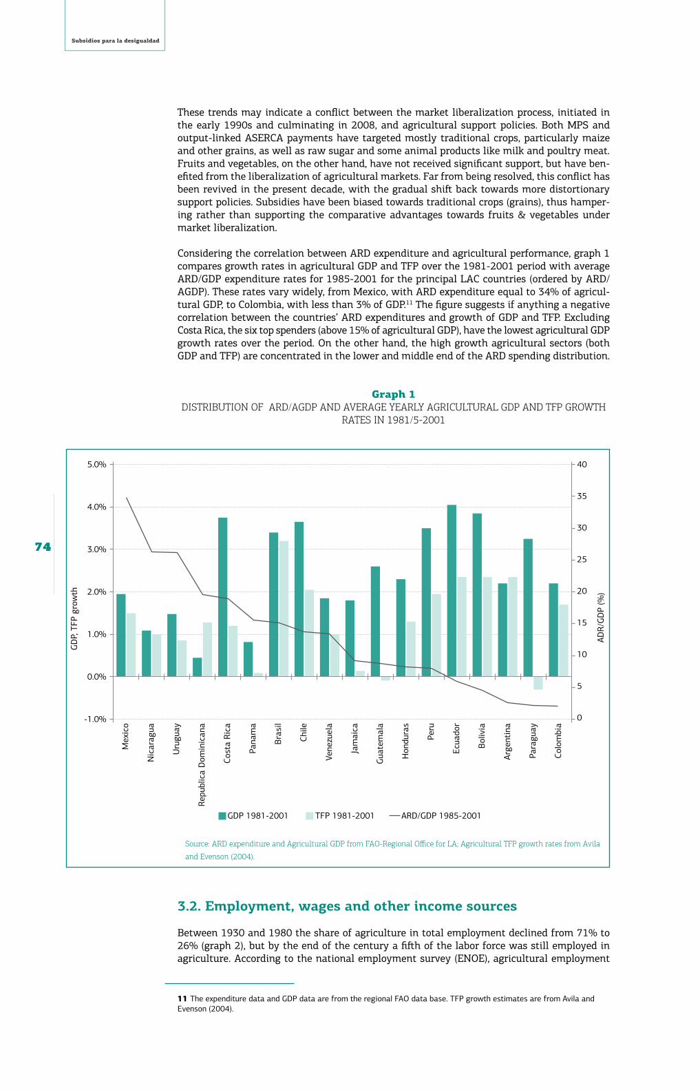
Considering the correlation between ARD expenditure and agricultural performance, graph 1 compares growth rates in agricultural GDP and TFP over the 1981-2001 period with average ARD/GDP expenditure rates for 1985-2001 for the principal LAC countries (ordered by ARD/AGDP). These rates vary widely, from Mexico, with ARD expenditure equal to 34% of agricul-tural GDP, to Colombia, with less than 3% of GDP.11 The figure suggests if anything a negative correlation between the countries’ ARD expenditures and growth of GDP and TFP. Excluding Costa Rica, the six top spenders (above 15% of agricultural GDP), have the lowest agricultural GDP growth rates over the period. On the other hand, the high growth agricultural sectors (both GDP and TFP) are concentrated in the lower and middle end of the ARD spending distribution.
Graph 1Distribution of ArD/AGDP AnD AverAGe yeArly AGriculturAl GDP AnD tfP Growth
rAtes in 1981/5-2001
source: ArD expenditure and Agricultural GDP from fAo-regional office for lA; Agricultural tfP growth rates from Avila
and evenson (2004).
3.2.Employment,wagesandotherincomesources
Between 1930 and 1980 the share of agriculture in total employment declined from 71% to 26% (graph 2), but by the end of the century a fifth of the labor force was still employed in agriculture. According to the national employment survey (ENOE), agricultural employment
11 The expenditure data and GDP data are from the regional FAO data base. TFP growth estimates are from Avila and Evenson (2004).
-1.0%
0.0%
1.0%
2.0%
3.0%
4.0%
5.0%
Mex
ico
Nic
arag
ua
Uru
guay
Repu
blic
a D
omin
ican
a
Cost
a Ri
ca
Pana
ma
Bra
sil
Chile
Vene
zuel
a
Jam
aica
Gua
tem
ala
Hon
dura
s
Peru
Ecua
dor
Bol
ivia
Arge
ntin
a
Para
guay
Colo
mbi
a
40
35
30
25
20
15
10
5
0
GD
P, T
FP g
row
th
ADR/
GD
P (%
)
GDP 1981-2001 TFP 1981-2001 ARD/GDP 1985-2001

3
Agricultural Subsidies in Mexico
75
has declined to 13% in 2008, representing 5.7 million workers, but is still very significant in the poor southern states: 40% in Chiapas, and close to 30% in Oaxaca and Guerrero.
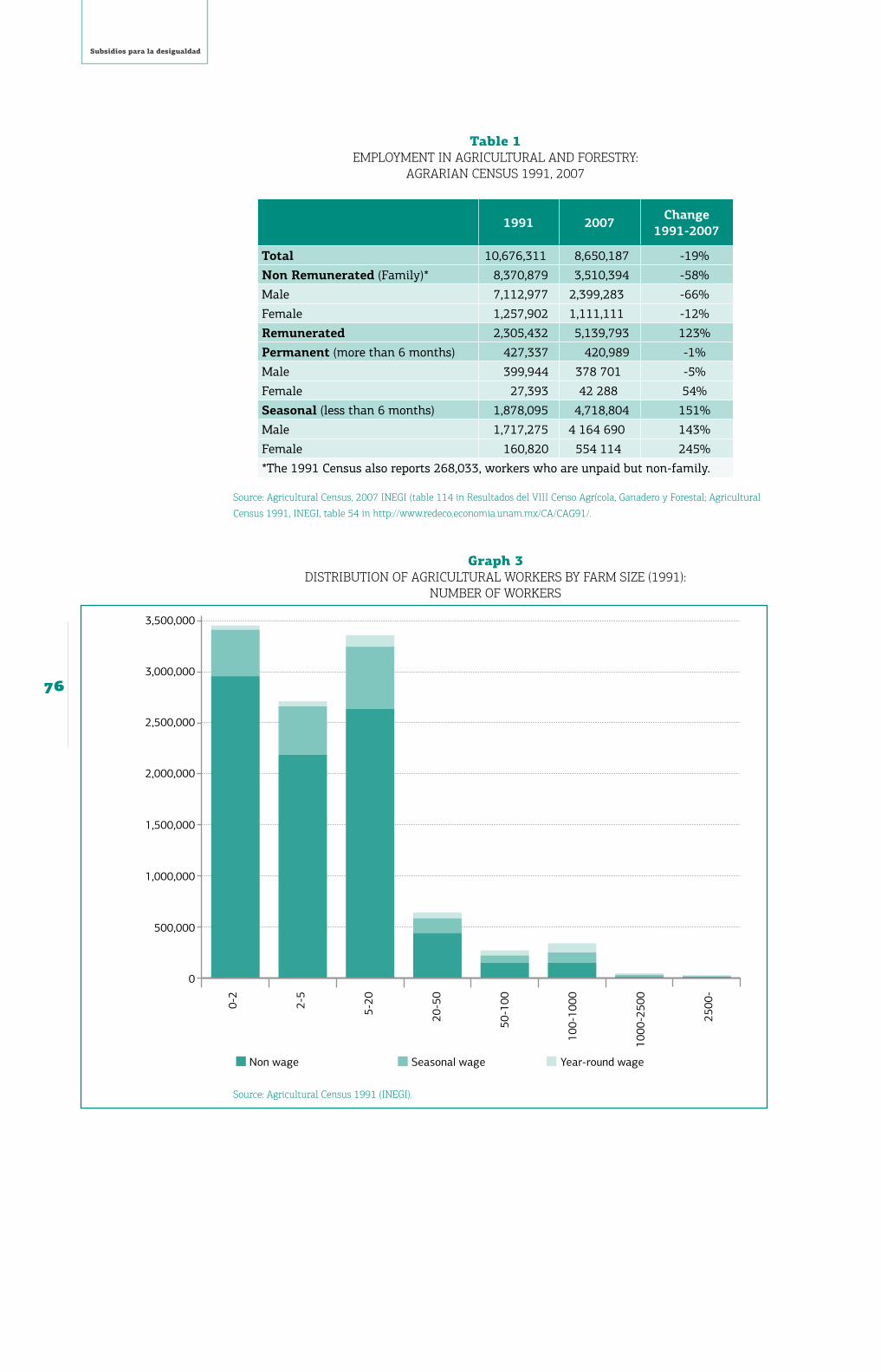
Despite these employment data, the economic weight and labor income from agriculture has fallen drastically in recent decades. The 2007 Agricultural Census shows that most workers in the sector are unpaid family members, and of those who receive payment the majority are eventual workers (Table 1): of the 8.6 million persons reported working in agriculture in the 2007 Census, only 421,000 are permanent paid workers. This number has practically remained the same since the 1991 Census, while the total number of workers has declined from 10.6 to 8.6 million, and unpaid family workers have declined from 8.3 to 3.5 million, with seasonal paid workers increasing from 1.8 to 4.7 million. This substitution of unpaid family workers for paid seasonal workers is striking and suggests agricultural labor markets have developed sig-nificantly in the NAFTA years, liberating family members for more productive rural and non-rural employment (migration) opportunities. This hypothesis is also consistent with the evolu-tion of rural income sources, described in the next section (see graph 10, 11).
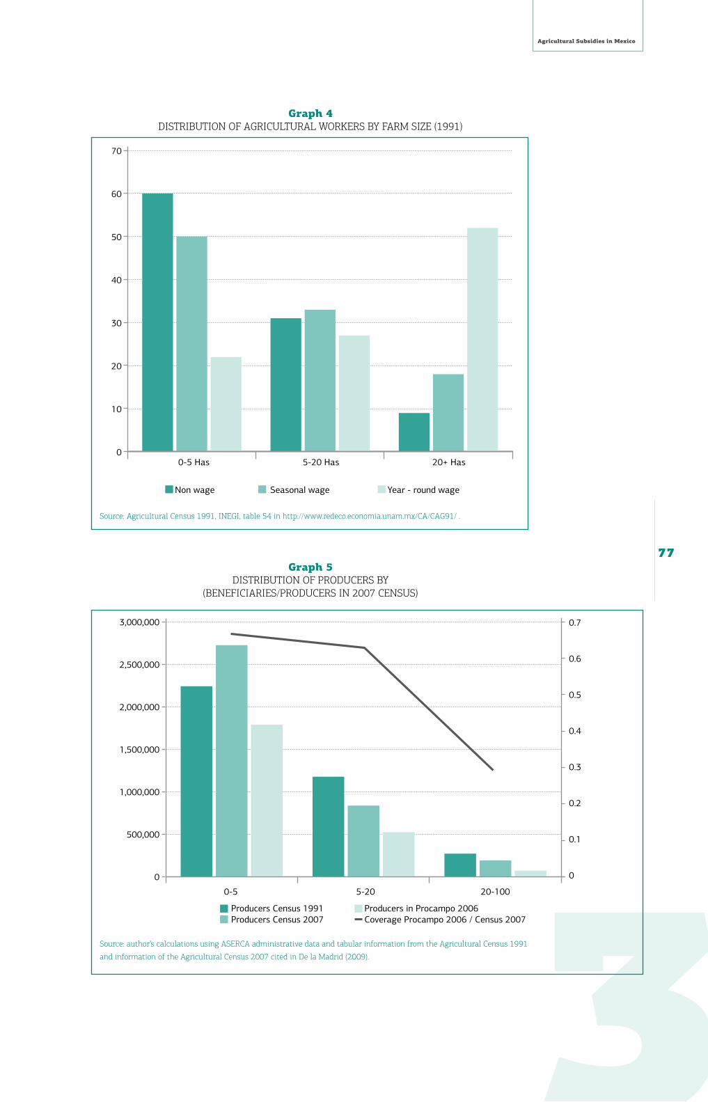
Unfortunately, at the time of writing the tables from the 2007 Agricultural Census published by INEGI do not report employment by farm size. However, the data from the 1991 Census (graphs 3, 4) shows that both unpaid family workers and paid seasonal workers are concen-trated in small to medium farms, while paid workers are concentrated in medium to large farms. Comparing the number of producers in each strata (graph 5), it is interesting to note that between 1991 and 2007 small producers have increased from 2.24 to 2.75 million, while the number of both middle-sized and larger producers have declined by almost 30%.
Wages in the primary sector have also fallen significantly in relation to the rest of the econo-my and even in absolute terms (table 2, graph 6), declining by 2.2% annually in 1989-1994 while average wages for the economy overall increased 6% annually, and increasing 1.4% an-nually in the last decade (vs. 2.9% overall). The decline in primary sector employment deceler-ated in 2007-2008, and wages actually increased more than in the rest of the economy in this year. The primary sector only accounted for 6% of the total wage mass of the economy in 2008.
Graph 2emPloyment in AGriculture As A shAre of totAl emPloyment in mexico:
nAtionAl AnD selecteD stAtes
source: ineGi; Population census: 1930-1990; enoe; 1996-2008.
0
10
20
30
40
50
60
70
80
90
100
1930
1940
1950
1960
1970
1980
1990
1996
1998
1999
2000
2001
2002
2003
2004
2005
2006
2007
2008
Nacional Chiapas Oaxaca Guerrero Sonora Chihuahua Sinaloa Tamaulipas México
Subsidios para la desigualdad
76
Table 1emPloyment in AGriculturAl AnD forestry:
AGrAriAn census 1991, 2007
1991 2007Change1991-2007
Total 10,676,311 8,650,187 -19%
NonRemunerated (Family)* 8,370,879 3,510,394 -58%
Male 7,112,977 2,399,283 -66%
Female 1,257,902 1,111,111 -12%
Remunerated 2,305,432 5,139,793 123%
Permanent (more than 6 months) 427,337 420,989 -1%
Male 399,944 378 701 -5%
Female 27,393 42 288 54%
Seasonal (less than 6 months) 1,878,095 4,718,804 151%
Male 1,717,275 4 164 690 143%
Female 160,820 554 114 245%
*The 1991 Census also reports 268,033, workers who are unpaid but non-family.
source: Agricultural census, 2007 ineGi (table 114 in resultados del viii censo Agrícola, Ganadero y forestal; Agricultural
census 1991, ineGi, table 54 in http://www.redeco.economia.unam.mx/cA/cAG91/.
Graph 3Distribution of AGriculturAl workers by fArm size (1991):
number of workers
source: Agricultural census 1991 (ineGi).
0
500,000
1,000,000
1,500,000
2,000,000
2,500,000
3,000,000
3,500,000
Non wage Seasonal wage Year-round wage
0-2
2-5
5-20
20-5
0
50-1
00
100-
1000
1000
-250
0
2500
-
3
Agricultural Subsidies in Mexico
77
Graph 4Distribution of AGriculturAl workers by fArm size (1991)
source: Agricultural census 1991, ineGi, table 54 in http://www.redeco.economia.unam.mx/cA/cAG91/ .
Graph 5Distribution of ProDucers by
(beneficiAries/ProDucers in 2007 census)
source: author’s calculations using AsercA administrative data and tabular information from the Agricultural census 1991
and information of the Agricultural census 2007 cited in De la madrid (2009).
0
10
20
30
40
50
60
70
0-5 Has 5-20 Has 20+ Has
Non wage Seasonal wage Year - round wage
0-5 5-20 20-100
0
500,000
1,000,000
1,500,000
2,000,000
2,500,000
3,000,000 0.7
0.6
0.5
0.4
0.3
0.2
0.1
0
Producers Census 1991 Producers in Procampo 2006Producers Census 2007 Coverage Procampo 2006 / Census 2007

Subsidios para la desigualdad
78
Table 2emPloyment AnD wAGes in PrimAry sector:
2005-2008 (first quArter)
Primary Sector Other sectors
Employed pop
2005 6,047,361 34,528,5132006 5,875,619 35,845,4962007 5,734,735 36,665,727
2008 5,676,086 37,644,591
Wage (MP/month)
2005 2,605 10,1472006 2,393 10,5952007 2,293 10,8652008 2,382 11,121
Annual growth rates
Employed Pop2005-2006 -2.8% 3.8%2006-2007 -2.4% 2.3%2007-2008 -1.0% 2.7%
Wage2005-2006 -8.1% 4.4%2006-2007 -4.2% 2.6%2007-2008 3.9% 2.4%
Wage Mass2005-2006 -10.7% 8.4%2006-2007 -6.5% 4.9%2007-2008 2.8% 5.1%
source: enoe 2005-2008, ineGi.
Graph 6AnnuAl chAnGe in wAGes: 1988-2008
source: ene, enoe.
4. rural Poverty and InequalIty;agrIculture In rural IncomesMeasuring rural development in terms of monetary poverty and basic human development in dicators, large gaps persist between the rural and urban sector, but also within the rural sector. Extreme poverty (alimentaria) declined from 53% to 24% between 1996 and 2006, but most of this decline represents a recovery from the dramatic increase in poverty following the 1995 “tequila” crisis: the 1992-2002 decade was fully “lost” in terms of rural poverty-reduc-
Agriculture Total
- 2.2 %
6.0 %
-12.2 % -11.3 %
1.4 %
2.5 %
1989-1994 1995-1996 1997-2008-15
-10
-5
0
5
10
3
Agricultural Subsidies in Mexico
79
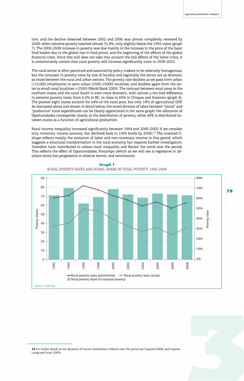
tion, and the decline observed between 2002 and 2006 was almost completely reversed by 2008, when extreme poverty reached almost 31.8%, only slightly below the 1992 value (graph 7). The 2006-2008 increase in poverty was due mainly to the increase in the price of the basic food basket due to the global rise in food prices, and the beginning of the effects of the global financial crisis. Since this still does not take into account the full effects of the latter crisis, it is unfortunately certain that rural poverty will increase significantly more in 2009-2010.
The rural sector is often perceived and assumed by policy makers to be relatively homogenous, but the contrasts in poverty rates by size of locality and regionally the sector are as dramatic as those between the rural and urban sectors. The poverty rate doubles as we pass from urban (>15,000 inhabitants) to semi-urban (2500-15000) localities, and doubles again from the lat-ter to small rural localities (<2500) (World Bank 2005). The contrast between rural areas in the northern states and the rural South is even more dramatic, with almost a ten-fold difference in extreme poverty rates: from 6.5% in BC, to close to 60% in Chiapas and Guerrero (graph 8). The poorest eight states account for 64% of the rural poor, but only 18% of agricultural GDP. As discussed above and shown in detail below, the noted division of labor between “social” and “productive” rural expenditures can be clearly appreciated in the same graph: the allocation of Oportunidades corresponds closely to the distribution of poverty, while APE is distributed be-tween states as a function of agricultural production.
Rural income inequality increased significantly between 1994 and 2000 (2002 if we consider only monetary income sources), but declined back to 1994 levels by 2006).12 The inverted U-shape reflects mostly the evolution of labor and non-monetary income in this period, which suggests a structural transformation in the rural economy but requires further investigation. Transfers have contributed to reduce rural inequality and flatten the trend over the period. This reflects the effect of Oportunidades, Procampo (which as we will see is regressive in ab-solute terms but progressive in relative terms), and remittances.
Graph 7rurAl Poverty rAtes AnD rurAl shAre in totAl Poverty: 1992-2006
source: conevAl.
12 For further details on the dynamics of income distribution in Mexico over this period see Esquivel (2008), and Esquivel, Lustig and Scott (2009).
Rural poverty rates (patrimonial) Rural poverty rates (acute)Rural poverty share (in national poverty)
80%
70%
60%
50%
40%
30%
20%
10%
0%
1992
1994
1996
1998
2000
2002
2004
2005
2006
2008
Pove
rty
shar
es
Pove
rty
rate
s
0
10
20
30
40
50
60
70
80
90

Subsidios para la desigualdad
80
Graph 8extreme rurAl Poverty (PobrezA AlimentAriA), AGDP AnD Public ArD
exPenDiture: 2005/2006(stAtes orDereD by extreme rurAl Poverty rAte)
source: conevAl (rural poverty); ineGi (Agricultural GDP); oliver and santillanes (2008): (ArD expenditure.
Extreme inequalities in rural living standards persist even in the basic human development (health, education) indicators targeted by the principal social spending programs. In the 2000 census, illiteracy in rural areas was 21%, twice the national average and seven times the aver-age for Mexico City, and average schooling was less than 5 years, half the average for Mexico City. Almost three-quarters of the population in Mexico City (half of the national population) had completed post-primary education, but only a quarter of the population in the rural sec-tor. In 2005, infant mortality rates (IMR) varied widely by municipality ordered by the CO-NAPO marginality index, a multi-dimensional poverty indicator closely correlated with degree of “ruralness”: from 3-8 per thousand (live births) in richer urban delegaciones, to 30-80 per thousand in the poorest municipalities, comparable to the gap observed between low and high income countries in the world (graph 9).
To assess the extent to which agriculture offers income and employment opportunities for the rural poor in Mexico, we use ENIGH income-expenditure surveys, the ENOE (2008) employ-ment survey, and ENCASEH (2004), a large and detailed survey covering households in Opor-tunidades localities. Though the latter is not nationally representative, it is representative of producers in poor rural localities.
There has been a dramatic transformation in the income sources for the average rural house-hold over the last decade. Independent (non-wage) farm income has collapsed from 28.7% to 9.1% of total household income between 1992 and 2004, while total (independent and wage) farm income has contracted from close to 38% to just 17% of household income (graph 10).
The extreme rural poor have a larger participation in agricultural activities, but they also de-rive a relatively small share of their income from the sector (graphs 11 and 12, tables 3 and 4). The poorest quintile accounts for more than half of all agricultural workers and 60% of house-
0
10
20
30
40
50
60
Rural poverty rate
Cumulative poverty shares Cumulative Agric. GDP
Cumulative Oportunidades shares Cumulative APE shares
Chia
pas
Gue
rrer
o
Oax
aca
San
Luis
Pot
osí
Pueb
la
Vera
cruz
Taba
sco
Mic
hoac
án
Cam
pech
e
Dur
ango
Gua
naju
ato
Hid
algo
Qui
ntan
a Ro
o
Yuca
tán
Méx
ico
Nay
arit
Zaca
teca
s
Tam
aulip
as
Sina
loa
Que
réta
ro
Chih
uahu
a
Jalis
co
Sono
ra
Tlax
cala
Coah
uila
Agua
scal
ient
es
Nue
vo L
eón
Mor
elos
Colim
a
Baj
a Ca
lifor
nia
Sur
Dis
trit
o Fe
dera
l
Baj
a Ca
lifor
nia
Pove
rty
rate
Cum
mul
ativ
e sh
ares

3
Agricultural Subsidies in Mexico
81
holds in the poorest decile have agricultural workers, though only 26.6% of these households report generating independent farming income. However, the poorest 30% of households ob-tain on average less than a third of their income from agriculture. In particular, subsistence farming has become irrelevant source of income for rural households: 27% of HHs report ob-taining non-monetary income from self-production/consumption, but this represents less than 2% of their total current income, and only 7% for the poorest decile. Non-farming wages represents the principal single income source for all but the poorest decile, whose largest in-come source are public transfers.
In comparison to urban households, rural households obtain a smaller share of their income from the labor market (41%) and are more dependent on transfers (18%) and self-employment (18%).
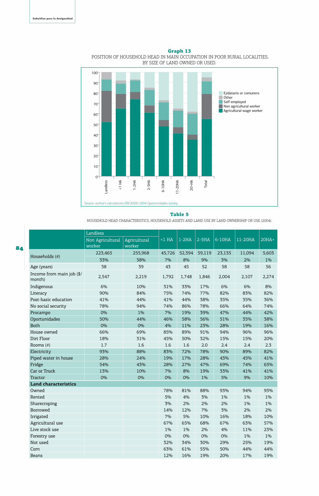
Considering the characteristics of rural households in poor localities were Oportunidades op-erates, table 4 divides these by land-holdings. It is notable first that 71% of these households are landless. Though these households tend to be younger and have less assets generally (housing, appliances and cars), they also report higher labor income and education indicators than land owners.
Among the latter non-agricultural workers are better off than agricultural workers, which also report the lowest coverage of social security of all household groups (5%).
By far the poorest households in these localities are not the landless, but small-holders, espe-cially households with less than 2 hectares. These also tend to have a higher proportion of indigenous population and agricultural workers (more than 70% of these household report the main occupation of the household head as agricultural workers), but lowest proportion of eji-datarios or comuneros.
The great majority of land-holders own their land, though this proportion is lower for small holders. Most of the land is rainfed, though the proportion of irrigated land increases in the 6-20 ha range. Corn is the principal crop, especially among small-holders, followed by beans.
The data on the coverage of public programs will be taken up in section 6.
Graph 9infAnt mortAlity rAtes (imr) by municiPAlities orDereD by imr AnD conAPo
mArGinAlity inDex: 2005
source: conAPo.
80
70
60
50
40
30
20
10
0
Ordered by Conapo Marginality Index Ordered by IMR (2005)
Urban, low marginalityRural, high marginality

Subsidios para la desigualdad
82
Graph 10income sources of rurAl householDs: 1992-2004
source: ruiz castillo (2005). total does not add up to 100% because smaller or unspecified income sources were excluded.
Graph 11income sources of rurAl AnD AGriculturAl householDs: 2006
(income Por cAPitA Per month)
source: author’s calculations based on eniGh 2006 (ineGi).
Independent FarmingAgricultural Wage LaborIndep. Non-Farm Activs. Non-Farm Wage LaborPensionsInternational transfers Oportunidades and Procampo transfers Domestic inter-household transfers
0
10
20
30
40
50
60
70
80
90
100
1992 2004
28.7
9.0
15.5
22.8
0.11.62.0
8.6
9.1
8.2
18.5
36.3
3.74.14.24.6
Farmincome
Non farmincome
Transfers
0
10
20
30
40
50
60
70
80
90
100
OtherAutoconsumoIn kind payments and gistsPublic transfers Private transfers Independent Income Non FarmingWages Non FarmingIndependent Income FarmingWages Farming
1 2 3 4 5 6 7 8 9 10

3
Agricultural Subsidies in Mexico
83
Table 3AGriculturAl Activities by rurAl householD Deciles orDereD by income Per cAPitA (2006)
Hh with agricultural workers Hh with independent farming income
HH Deciles Households % DecileHouse-holds
% DecileAnnual farming income
million MP MP/hh
1 3,222,510 60% 705,977 26.6% 2,705 3,8312 1,492,371 32% 249,587 9.4% 1,830 7,3313 946,424 24% 190,263 7.2% 1,253 6,5864 625,353 15% 119,835 4.5% 1,038 8,6645 578,002 13% 103,074 3.9% 1,853 17,9776 340,805 9% 86,394 3.3% 982 11,3627 390,019 9% 68,100 2.6% 977 14,3498 233,630 7% 63,465 2.4% 917 14,4569 144,672 5% 30,022 1.1% 878 29,24910 152,976 4% 39,521 1.5% 3,521 89,093Total 8,126,762 18% 1,656,238 6.2% 15,954 9,633
source: author’s estimations based on eniGh (2006).
Table 4monetAry AnD non-monetAry (nm) income sources: rurAl AnD urbAn hh:
% of totAl current income (2006)
Urban Rural
HH Income HH IncomeLabor income 79% 52% 67% 41%Independent income 38% 15% 53% 18%Transfers 38% 9% 70% 18%Presents (NM) 70% 8% 71% 11%Implicit housing rent (NM) 80% 12% 95% 9%Self-production/consumption (NM) 12% 0.7% 27% 1.8%Payments in kind (NM) 18% 1.6% 6.6% 0.9%Rent 6.0% 3.4% 3.2% 0.9%
source: eniGh 2006
Graph 12Public AnD PrivAte trAnsfers Per cAPitA Per month receiveD
by rurAl householDs: 2006 (by Decile)
source: author’s calculations based on eniGh 2006 (ineGi).
1 2 3 4 5 6 7 8 9 100
100
200
300
400
500
600
PROCAMPOOportunidadesInternational private transfers Domestic private transfersOther public transfersOld Age Pensions
Subsidios para la desigualdad
84
Graph 13 Position of householD heAD in mAin occuPAtion in Poor rurAl locAlities,
by size of lAnD owneD or useD.
source: author’s calculations encAseh 2004 oportunidades survey.
Table 5householD heAD chArActeristics, householD Assets AnD lAnD use by lAnD ownershiP or use (2004).
Landless<1 HA 1-2HA 2-5HA 6-10HA 11-20HA 20HA+Non Agricultural
workerAgriculturalworker
Households (#)223,465 255,968 45,726 52,394 59,119 23,135 11,094 5,603
33% 38% 7% 8% 9% 3% 2% 1%Age (years) 38 39 43 45 52 58 58 56
Income from main job ($/month) 2,547 2,219 1,792 1,748 1,846 2,004 2,107 2,274
Indigenous 6% 10% 31% 33% 17% 6% 6% 8%Literacy 90% 84% 75% 74% 77% 82% 83% 82%Post-basic education 41% 44% 41% 44% 38% 35% 35% 36%No social security 78% 94% 74% 86% 78% 66% 64% 74%Procampo 0% 1% 7% 19% 39% 47% 44% 42%Oportunidades 50% 44% 46% 58% 56% 51% 35% 38%Both 0% 0% 4% 11% 23% 28% 19% 16%House owned 66% 69% 85% 89% 91% 94% 96% 96%Dirt Floor 18% 31% 45% 50% 32% 15% 15% 20%Rooms (#) 1.7 1.6 1.6 1.6 2.0 2.4 2.4 2.3Electricity 93% 88% 83% 72% 78% 90% 89% 82%Piped water in house 28% 24% 19% 17% 28% 43% 45% 41%Fridge 54% 43% 28% 27% 47% 69% 74% 65%Car or Truck 13% 10% 7% 8% 19% 33% 41% 41%Tractor 0% 0% 0% 0% 1% 5% 9% 10%LandcharacteristicsOwned 78% 81% 88% 93% 94% 95%Rented 5% 4% 3% 1% 1% 1%Sharecroping 3% 2% 2% 2% 1% 1%Borrowed 14% 12% 7% 3% 2% 2%Irrigated 7% 5% 10% 16% 18% 10%Agricultural use 67% 65% 68% 67% 63% 57%Live stock use 1% 1% 2% 4% 11% 23%Forestry use 0% 0% 0% 0% 1% 1%Not used 32% 34% 30% 29% 25% 19%Corn 63% 61% 55% 50% 44% 44%Beans 12% 16% 19% 20% 17% 19%
0
10
20
30
40
50
60
70
80
90
100
Ejidatario or comuneroOtherSelf-employedNon agricultural workerAgricultural wage worker
Land
less
<1 H
A
1-2H
A
2-5H
A
6-10
HA
11-2
0HA
20+H
A
Tota
l

3
Agricultural Subsidies in Mexico
85
5. geograPHIc dIstrIbutIon oFagrIcultural subsIdIes 5.1Distributionofagriculturalpublicexpendituresacrossstates
The geographic analysis agricultural public expenditures (APE) is presented at the state level for most programs, but extended to the municipality level where information is available (Pro-campo, Ingreso Objetivo). In this case the distribution of APE is analyzed ordering states (and municipalities) by their rural poverty rates, using the official measures of pobreza alimentaria estimated by CONEVAL for 2005 (see graph 8 above), except for graph 14 which uses the mul-tivariate CONAPO marginality index. The two state rankings are closely correlated.
The division of labor between social and productive programs noted above (section 2) is illus-trated clearly by the overall allocation of these programs at the state level. Graph 8 (section 4 above) compares the cumulative distribution of APE and of Oportunidades, the largest rural social program. This reveals that the distribution of APE follows closely the distribution agri-cultural GDP (AGDP), while the distribution of Oportunidades follows closely the distribution of extreme rural poverty.
The correlation of APE with agricultural economic activity is weaker if we consider agricul-tural employment (PO Agr in graph 14). As we have seen before, the largest beneficiaries, the richer agricultural states of Sinaloa, Tamaulipas, Chihuahua and Jalisco, account for a rela-tively small proportion of agricultural employment. By contrast, the poorer states of Veracruz, Chiapas, Oaxaca, Puebla and Guerrero, account for a large part of employment but receive a much smaller share of these resources.
The distribution of APE per rural capita for the principal programs is concentrated in the richer half of the poverty-ordered state distribution, with the highest benefits allocated to Tamaulipas, Sinaloa, Chihuahua, and Sonora (graph 15, using data presented in World Bank 2004). These four states are among the principal beneficiaries of Procampo (in per capita terms), reflecting their agricultural land assets, but their disproportionate participation in APE is also explained by Apoyos, Diesel and the electricity/water subsidies (Tarifa 9). At the other extreme of the state distribution, the poorest states obtain support mostly from Procampo and Alianza, but overall obtain barely a tenth of the support benefiting the former states (in rural per capita terms).
Graph 14AGriculturAl Public exPenDiture (APe), AGriculturAl GDP (AGDP) AnD
AGriculturAl emPloyment (Po AGr)
source: author’s calculations based on Agricultural census 1991 (ineGi).
0
2
4
6
8
10
12
14
Sina
loa
Tam
aulip
asCh
ihua
hua
Jalis
coSo
nora
Vera
cruz
Zaca
teca
sCh
iapa
sG
uana
juat
oM
icho
acán
Dur
ango
Oax
aca
Pueb
laM
éxic
oSa
n Lu
is P
otos
íG
uerr
ero
Baj
a Ca
lifor
nia
Hid
algo
Coah
uila
Taba
sco
Nue
vo L
eón
Nay
arit
Cam
pech
eYu
catá
nTl
axca
laQ
ueré
taro
Mor
elos
Colim
aAg
uasc
alie
ntes
Baj
a Ca
lifor
nia
Sur
Qui
ntan
a Ro
oD
istr
ito
Fede
ral
APE AGDP PO Ag

Subsidios para la desigualdad
86
Graph 15AnnuAl sPenDinG Per rurAl cAPitA (mP) by PrinciPAl APe ProGrAms:
2006 (2002) (stAtes orDereD by extreme Poverty rAte)
source: oliver and santillanes (2008
The electricity subsidy for agriculture is mostly used for water-pumping for irrigation in the northern states and represented 10,672 million pesos in 2008 (Tercer Informe de Gobierno, 2009). This is the most heavily subsidized use of electricity in Mexico, with price equal to just 28% of cost (vs. 90-100% in industry). In addition to its regressive allocation, which is a con-sequence of the distribution of hydrological resources in Mexico, this subsidy has contributed to a significant and unsustainable increase in the over-exploitation of aquifers in Mexico (Mu-ñoz et al. 2005, Guevara et al. 2007, Kessler et al 2007).
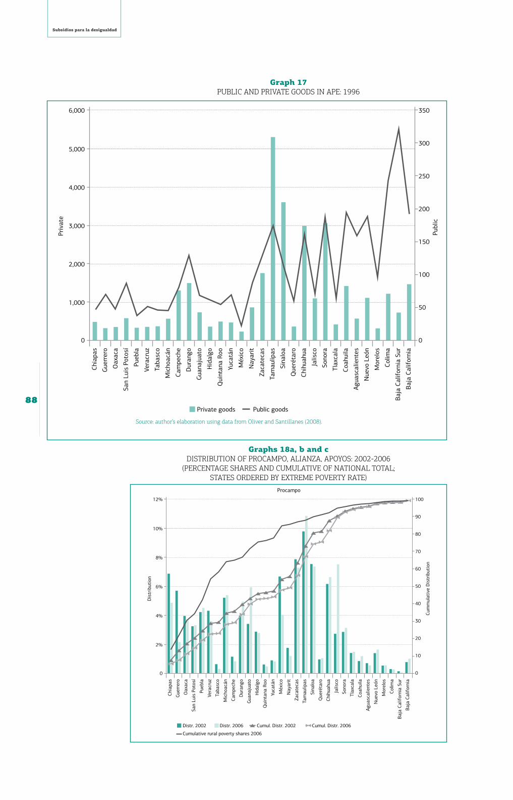
Taking the broadest division between public goods, representing less than 10% of total agri-cultural public spending (see graph 17), and private transfers, it is notable that the former are even more regressively distributed than the latter, with per capita benefits rising significantly in the upper half of the state distribution.
Considering the distribution of the three principal support programs, Procampo, Alianza and Apoyos (graph 18, the cumulative distribution of extreme poverty is included as a benchmark to judge the degree of progressivity of the programs), Alianza is the most progressive at the state level, with 28% of transfers going to the poorest five states, followed by Procampo, with 22%. The degree of progressivity has been slightly reduced for both programs between 2002 and 2006. Apoyos is highly concentrated in just four states, Sinaloa, Sonora, Tamaulipas en Chihuahua receiving 80% of its resources in 2002, with the poorest half of the states receiving just 5% of resources in 2002, and less than 10% in 2006.
Considering the case of Procampo in particular, we use the 1991 and 2007 Agricultural Census to evaluate coverage at the state level (graphs 20-22a), in the PV cycle. This analysis must be interpreted with some care, as producers may be counted more than once in the Procampo data base, which may explain the coverage rates above 100% in smaller states. With this ca-veat, the analysis reveals a large variations in coverage between states, from full coverage in Durango and Coahuila, to less than 15% in BCS and Tabasco.
0
1,000
2,000
3,000
4,000
5,000
6,000
Alianza para el campo Diesel
Apoyos a la comercialización PROGAN PROCAMPO (Traditional)
Chia
pas
Gue
rrer
o
Oax
aca
San
Luis
Pot
osí
Pueb
la
Vera
cruz
Taba
sco
Mic
hoac
án
Cam
pech
e
Dur
ango
Gua
naju
ato
Hid
algo
Qui
ntan
a Ro
o
Yuca
tán
Méx
ico
Nay
arit
Zaca
teca
s
Tam
aulip
as
Sina
loa
Que
réta
ro
Chih
uahu
a
Jalis
co
Sono
ra
Tlax
cala
Coah
uila
Agua
scal
ient
es
Nue
vo L
eón
Mor
elos
Colim
a
Baj
a Ca
lifor
nia
Sur
Baj
a Ca
lifor
nia
Anua
l spe
ndin
g pe
r ru
ral c
apit
a

3
Agricultural Subsidies in Mexico
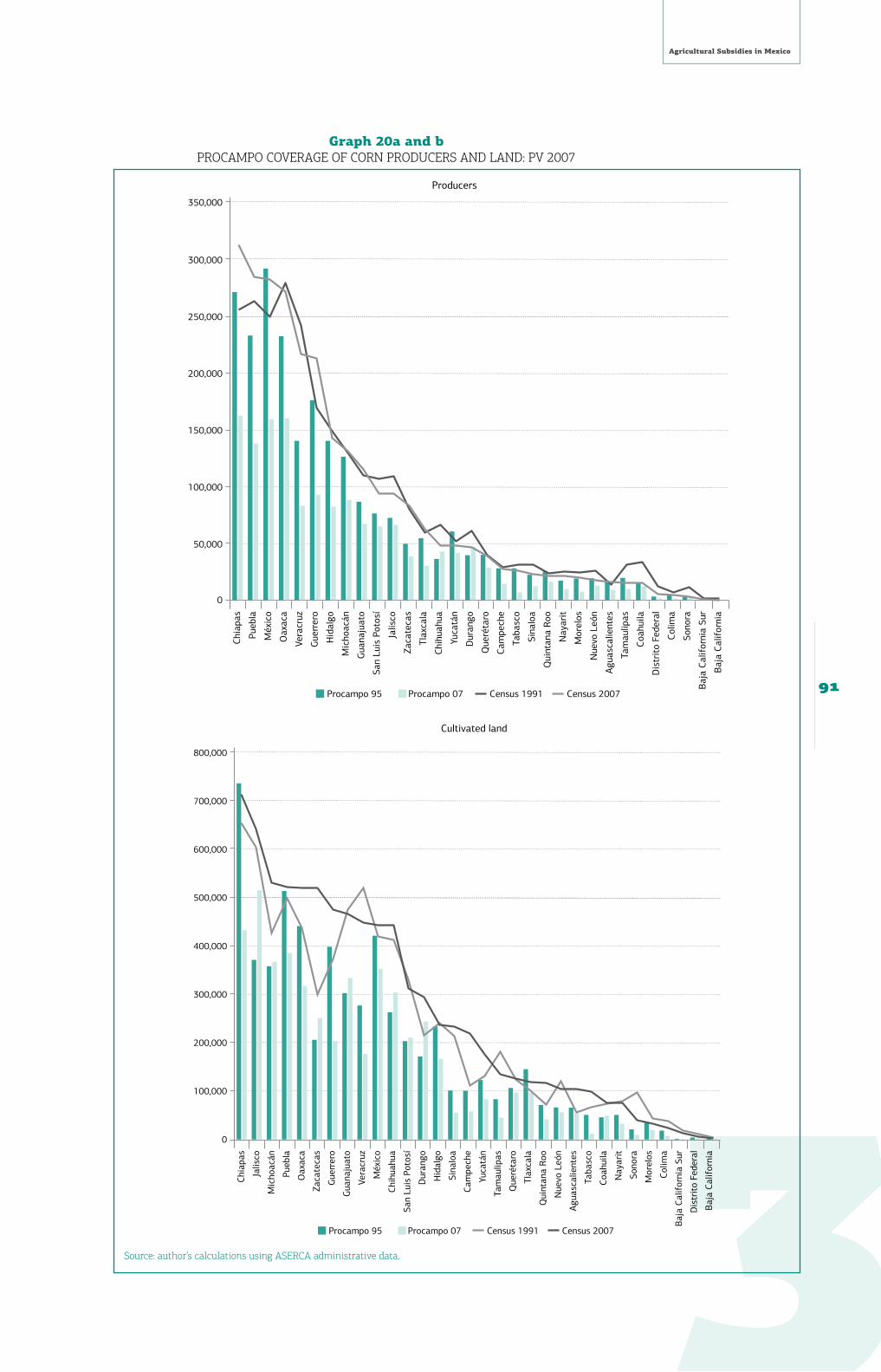
87
Considering the case of maize and comparing from the beginning to the present of the pro-gram (graph 20a), the number of producers has increased some states, including Chiapas, Puebla and México, but the total number of producers has decreased slightly (2.68 million in 1991, 2.66 million in 2007), while cultivated land has increased from 7.3 to 8.1 million hect-ares. Procampo’s coverage has decreased significantly in all states except Chihuahua, and Jalisco (in terms of land).
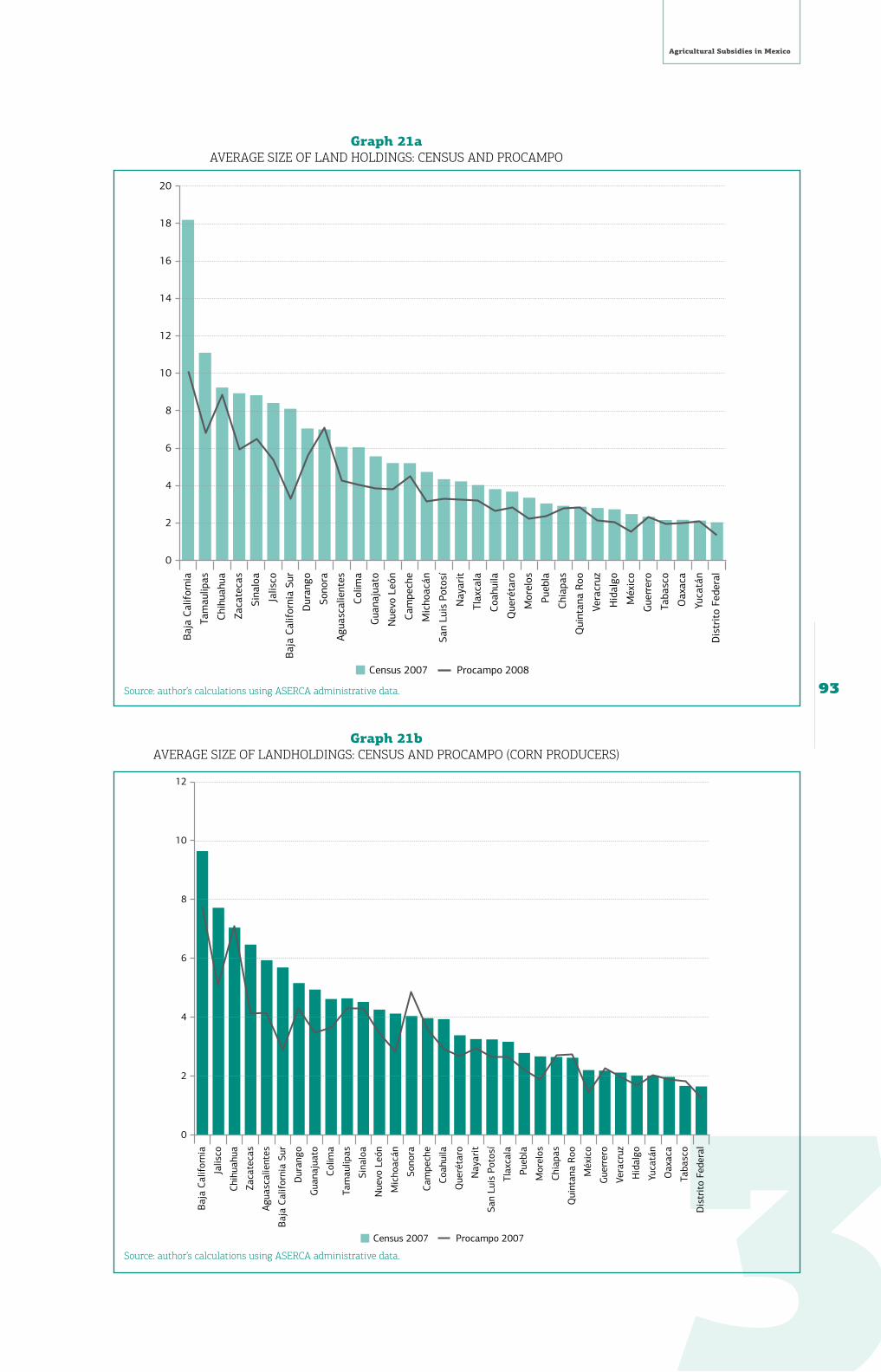
Procampo coverage is below 50% in the poorer states (Veracruz, Guerrero, Chiapas), and just above 50% in Oaxaca. Some of the large agricultural states have high coverage rates (Chihua-hua, Jalisco), but this is not so for Tamaulipas and Sinaloa. There appears to be no clear rela-tion with average size of land holdings (graph 21a).
Graph 16irriGAtion subsiDies
source: world bank (2004)
0
500
1,000
1,500
2,000
2,500
Agricultural electric subsidy Hydrological infrastructure Hydroagricultural infrastructure
Chia
pas
Gue
rrer
o
Oax
aca
San
Luis
Pot
osí
Pueb
la
Vera
cruz
Taba
sco
Mic
hoac
án
Cam
pech
e
Dur
ango
Gua
naju
ato
Hid
algo
Qui
ntan
a Ro
o
Yuca
tán
Méx
ico
Nay
arit
Zaca
teca
s
Tam
aulip
as
Sina
loa
Que
réta
ro
Chih
uahu
a
Jalis
co
Sono
ra
Tlax
cala
Coah
uila
Agua
scal
ient
es
Nue
vo L
eón
Mor
elos
Colim
a
Baj
a Ca
lifor
nia
Sur
Baj
a Ca
lifor
nia
Anua
l spe
ndin
g pe
r ru
ral c
apit
a
Subsidios para la desigualdad
88
Graph 17Public AnD PrivAte GooDs in APe: 1996
source: author’s elaboration using data from oliver and santillanes (2008).
Graphs 18a, b and cDistribution of ProcAmPo, AliAnzA, APoyos: 2002-2006
(PercentAGe shAres AnD cumulAtive of nAtionAl totAl;stAtes orDereD by extreme Poverty rAte)
0
1,000
2,000
3,000
4,000
5,000
Private goods Public goods
Chia
pas
Gue
rrer
o
Oax
aca
San
Luis
Pot
osí
Pueb
la
Vera
cruz
Taba
sco
Mic
hoac
án
Cam
pech
e
Dur
ango
Gua
naju
ato
Hid
algo
Qui
ntan
a Ro
o
Yuca
tán
Méx
ico
Nay
arit
Zaca
teca
s
Tam
aulip
as
Sina
loa
Que
réta
ro
Chih
uahu
a
Jalis
co
Sono
ra
Tlax
cala
Coah
uila
Agua
scal
ient
es
Nue
vo L
eón
Mor
elos
Colim
a
Baj
a Ca
lifor
nia
Sur
Baj
a Ca
lifor
nia
Priv
ate
Publ
ic
6,000
0
50
100
150
200
250
300
350
0
2%
4%
6%
8%
10%
Distr. 2002 Distr. 2006 Cumul. Distr. 2002 Cumul. Distr. 2006
Cumulative rural poverty shares 2006
Chia
pas
Gue
rrer
o
Oax
aca
San
Luis
Pot
osí
Pueb
la
Vera
cruz
Taba
sco
Mic
hoac
án
Cam
pech
e
Dur
ango
Gua
naju
ato
Hid
algo
Qui
ntan
a Ro
o
Yuca
tán
Méx
ico
Nay
arit
Zaca
teca
s
Tam
aulip
as
Sina
loa
Que
réta
ro
Chih
uahu
a
Jalis
co
Sono
ra
Tlax
cala
Coah
uila
Agua
scal
ient
es
Nue
vo L
eón
Mor
elos
Colim
a
Baj
a Ca
lifor
nia
Sur
Baj
a Ca
lifor
nia
Dis
trib
utio
n
Cum
mul
ativ
e D
istr
ibut
ion
12% 100
90
80
70
60
50
40
30
20
10
0
Procampo

3
Agricultural Subsidies in Mexico
89
source: author’s elaboration using data from oliver and santillanes (2008); world bank (2004).
0
20%
25%
10%
5%
15%
30%
35%
40%
Distr. 2002 Distr. 2006 Cumul. Distr. 2002 Cumul. Distr. 2006
Cumulative rural poverty shares 2006
Chia
pas
Gue
rrer
o
Oax
aca
San
Luis
Pot
osí
Pueb
la
Vera
cruz
Taba
sco
Mic
hoac
án
Cam
pech
e
Dur
ango
Gua
naju
ato
Hid
algo
Qui
ntan
a Ro
o
Yuca
tán
Méx
ico
Nay
arit
Zaca
teca
s
Tam
aulip
as
Sina
loa
Que
réta
ro
Chih
uahu
a
Jalis
co
Sono
ra
Tlax
cala
Coah
uila
Agua
scal
ient
es
Nue
vo L
eón
Mor
elos
Colim
a
Baj
a Ca
lifor
nia
Sur
Baj
a Ca
lifor
nia
Dis
trib
utio
n
Cum
mul
ativ
e D
istr
ibut
ion
45% 100
90
80
70
60
50
40
30
20
10
0
Apoyos
Chia
pas
Gue
rrer
o
Oax
aca
San
Luis
Pot
osí
Pueb
la
Vera
cruz
Taba
sco
Mic
hoac
án
Cam
pech
e
Dur
ango
Gua
naju
ato
Hid
algo
Qui
ntan
a Ro
o
Yuca
tán
Méx
ico
Nay
arit
Zaca
teca
s
Tam
aulip
as
Sina
loa
Que
réta
ro
Chih
uahu
a
Jalis
co
Sono
ra
Tlax
cala
Coah
uila
Agua
scal
ient
es
Nue
vo L
eón
Mor
elos
Colim
a
Baj
a Ca
lifor
nia
Sur
Baj
a Ca
lifor
nia
Dis
trib
utio
n
Cum
mul
ativ
e D
istr
ibut
ion
0
4%
5%
2%
1%
3%
6%
7%
8% 100
90
80
70
60
50
40
30
20
10
0
Distr. 2002 Distr. 2006 Cumul. Distr. 2002 Cumul. Distr. 2006
Cumulative rural poverty shares 2006
Alianza

Subsidios para la desigualdad
90
Graph 19ProcAmPo coverAGe of All AnD corn ProDucers Pv 2007
(beneficiAries/ProDucers in 2007 census)
source: author’s calculations using AsercA administrative data and 2007 Agricultural census, ineGi.
0
20%
40%
60%
80%
100%
120%
Dur
ango
Coah
uila
Chih
uahu
a
Jalis
co
Gua
naju
ato
Que
réta
ro
Yuca
tán
Zaca
teca
s
Qui
ntan
a Ro
o
Mic
hoac
án
Nue
vo L
eón
Tam
aulip
as
Agua
scal
ient
es
Hid
algo
Tlax
cala
San
Luis
Pot
osí
Méx
ico
Sina
loa
Oax
aca
Cam
pech
e
Sono
ra
Pueb
la
Chia
pas
Mor
elos
Colim
a
Gue
rrer
o
Nay
arit
Vera
cruz
Baj
a Ca
lifor
nia
Dis
trit
o Fe
dera
l
Baj
a Ca
lifor
nia
Sur
Taba
sco
140%
Total Corn
3
Agricultural Subsidies in Mexico
91
Graph 20a and bProcAmPo coverAGe of corn ProDucers AnD lAnD: Pv 2007
source: author’s calculations using AsercA administrative data.
0
50,000
100,000
150,000
200,000
250,000
300,000
Chia
pas
Pueb
la
Méx
ico
Oax
aca
Vera
cruz
Gue
rrer
o
Hid
algo
Mic
hoac
án
Gua
naju
ato
San
Luis
Pot
osí
Jalis
co
Zaca
teca
s
Tlax
cala
Chih
uahu
a
Yuca
tán
Dur
ango
Que
réta
ro
Cam
pech
e
Taba
sco
Sina
loa
Qui
ntan
a Ro
o
Nay
arit
Mor
elos
Nue
vo L
eón
Agua
scal
ient
es
Tam
aulip
as
Coah
uila
Dis
trit
o Fe
dera
l
Colim
a
Sono
ra
Baj
a Ca
lifor
nia
Sur
Baj
a Ca
lifor
nia
350,000
Procampo 95 Procampo 07 Census 1991 Census 2007
Producers
Chia
pas
Jalis
co
Mic
hoac
án
Pueb
la
Oax
aca
Zaca
teca
s
Gue
rrer
o
Gua
naju
ato
Vera
cruz
Méx
ico
Chih
uahu
a
San
Luis
Pot
osí
Dur
ango
Hid
algo
Sina
loa
Cam
pech
e
Yuca
tán
Tam
aulip
as
Que
réta
ro
Tlax
cala
Qui
ntan
a Ro
o
Nue
vo L
eón
Agua
scal
ient
es
Taba
sco
Coah
uila
Nay
arit
Sono
ra
Mor
elos
Colim
a
Baj
a Ca
lifor
nia
Sur
Dis
trit
o Fe
dera
l
Baj
a Ca
lifor
nia
600,000
500,000
800,000
700,000
400,000
300,000
200,000
100,000
0
Procampo 95 Procampo 07 Census 1991 Census 2007
Cultivated land

Subsidios para la desigualdad
92
5.2.Distributionofagriculturalpublicexpendituresacrossmunicipalities
We present an analysis of the distribution of transfers at the municipality level using admin-istrative ASERCA data for Procampo and Ingreso Objetivo (the principal instrument of Apoyos a la Comercialización), and data on the municipal allocation of most of the other ARD pro-grams included in PEC compiled by CEDRSSA (2009). Municipalities are ordered by acute rural poverty rates (pobreza alimentaria) estimated by CONEVAL.
Both Procampo and Ingreso Objetivo are regressively distributed, but the latter extremely so, with high per capita payments for a small fraction of municipalities, and no payments for most of the rest (graph 22a). In comparison, the Procampo benefits are densely distributed throughout. The poorest 50% of municipalities receive 40% of Procampo transfers, but less than 6% of Ingreso Objetivo, and in the latter case these resources are concentrated in a few municipalities so the great majority of the poorest half of municipalities (and all those in the poorest third) receive no transfers from Ingreso Objetivo at all.
The CEDRSSA (2009) data base allows for the first time an analysis of the distribution of a majority of the PEC programs, representing the bulk of federal ARD spending implemented in Mexico today. The data is for 2007 and covers 59 PEC programs with a combined budget of $104 billion pesos, representing close to 60% of PEC.
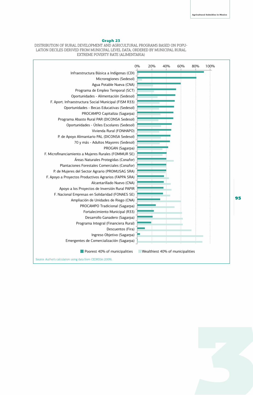
We analyze this data by ordering municipalities by rural poverty rates, partitioning municipal-ity sets thus ordered to obtain rural population deciles, so that each decile represents 10% of the rural population (not 10% of municipalities). Excluding some small programs and redun-dancies, graph 23 presents the distributions of 32 individual programs, and graph 24 presents the distribution of the programs grouped according to the principal functional categories.
Two important caveats in interpreting the following results must be mentioned. First, the quality of the data may vary significantly between programs, as they originate in administrative records. Secondly, the analysis ignores intra-municipal inequalities so the results may differ from the analysis based on individual producer or household data presented below (section 6).
Considering the programs individually, we find a wide range between the most progressive, Infraestructura Básica Indígena, with more than 90% allocated to the poorest 40%, and the most regressive, with 90% of resources allocated to the richest 40%. As expected, Sedesol pro-grams dominate among the more progressive, but we also find here indigenous (CDI), water (CAN), and transport (SCT) programs, as well as federalized funds (FAIIS) and Procampo Capi-taliza. The regressive end is dominated by Sagarpa Apoyos and Alianza programs, as well as financing programs (FIRA, Financiera Rural), FORTAMUN, and Procampo Tradicional. The contrast between Procampo Tradicional and Capitaliza is surprising and requires further investigation.
The distribution by functional categories (graph 24) confirms these results: social and infra-structure spending are progressive overall, environmental programs are broadly neutral, while financial and “competitiveness” programs (as these are classified in the PEC), are highly regres-sive. There is an interesting contrast between the two federalized municipal funds (Ramo 33): the FISM, allocated in part through a poverty-based formula, is progressive, while FORTAMUN is regressive. The overall distribution of all the PEC programs analyzed here is broadly neutral.13
13 See additional data in the full working paper version of this study.
3
Agricultural Subsidies in Mexico
93
Graph 21aAverAGe size of lAnD holDinGs: census AnD ProcAmPo
source: author’s calculations using AsercA administrative data.
Graph 21bAverAGe size of lAnDholDinGs: census AnD ProcAmPo (corn ProDucers)
source: author’s calculations using AsercA administrative data.
Census 2007 Procampo 2008
Baj
a Ca
lifor
nia
Tam
aulip
as
Chih
uahu
a
Zaca
teca
s
Sina
loa
Jalis
co
Baj
a Ca
lifor
nia
Sur
Dur
ango
Sono
ra
Agua
scal
ient
es
Colim
a
Gua
naju
ato
Nue
vo L
eón
Cam
pech
e
Mic
hoac
án
San
Luis
Pot
osí
Nay
arit
Tlax
cala
Coah
uila
Que
réta
ro
Mor
elos
Pueb
la
Chia
pas
Qui
ntan
a Ro
o
Vera
cruz
Hid
algo
Méx
ico
Gue
rrer
o
Taba
sco
Oax
aca
Yuca
tán
Dis
trit
o Fe
dera
l
0
20
18
14
10
6
16
12
8
4
2
Census 2007 Procampo 2007
Baj
a Ca
lifor
nia
Jalis
co
Chih
uahu
a
Zaca
teca
s
Agua
scal
ient
es
Baj
a Ca
lifor
nia
Sur
Dur
ango
Gua
naju
ato
Colim
a
Tam
aulip
as
Sina
loa
Nue
vo L
eón
Mic
hoac
án
Sono
ra
Cam
pech
e
Coah
uila
Que
réta
ro
Nay
arit
San
Luis
Pot
osí
Tlax
cala
Pueb
la
Mor
elos
Chia
pas
Qui
ntan
a Ro
o
Méx
ico
Gue
rrer
o
Vera
cruz
Hid
algo
Yuca
tán
Oax
aca
Taba
sco
Dis
trit
o Fe
dera
l
0
12
10
6
8
4
2

Subsidios para la desigualdad
94
Graphs 22a and bProcAmPo AnD inGreso objetivo trAnsfers in oi-2005 & Pv-2006 by municiPAlities
orDereD by rurAl extreme Poverty rAte (PobrezA AlimentAriA)
source: AsercA administrative data bases; conevAl municipal poverty measures.
5 80 155
230
305
380
455
530
605
680
755
830
905
980
1055
1130
1205
1280
1355
1430
1505
1580
1655
1730
1805
1880
1955
2030
2105
2180
2255
2330
2405
70%
100%
90%
80%
50%
60%
40%
30%
20%
10%
16,000
14,000
12,000
10,000
8,000
6,000
4,000
2,000
0
Procampo Pesos/cap Procampo cumulative distribution Cumulative rural poverty distribution
0
Procampo
5 80 155
230
305
380
455
530
605
680
755
830
905
980
1055
1130
1205
1280
1355
1430
1505
1580
1655
1730
1805
1880
1955
2030
2105
2180
2255
2330
2405
70%
90%
80%
50%
60%
40%
30%
20%
10%
4,500
4,000
3,500
3,000
2,500
2,000
1,500
1,000
500
0
100%
IO Pesos/cap IO cumulative distribution Cumulative rural poverty distribution
0
Ingreso - Objetivo
3
Agricultural Subsidies in Mexico
95
Graph 23Distribution of rurAl DeveloPment AnD AGriculturAl ProGrAms bAseD on PoPu-lAtion Deciles DeriveD from municiPAl level DAtA, orDereD by municiPAl rurAl
extreme Poverty rAte (AlimentAriA)
source: Author’s calculation using data from ceDrssA (2009).
Poorest 40% of municipalities Wealthiest 40% of municipalities
Infraestructura Básica a Indígenas (CDI)
Microregiones (Sedesol)
Agua Potable Nueva (CNA)
Programa de Empleo Temporal (SCT)
Oportunidades - Alimentación (Sedesol)
F. Aport. Infraestructura Social Municipal (FISM R33)
Oportunidades - Becas Educativas (Sedesol)
PROCAMPO Capitaliza (Sagarpa)
Programa Abasto Rural PAR (DICONSA Sedesol)
Oportunidades - Útiles Escolares (Sedesol)
Vivienda Rural (FONHAPO)
P. de Apoyo Alimantario PAL (DICONSA Sedesol)
70 y más - Adultos Mayores (Sedesol)
PROGAN (Sagarpa)
F. Microfinanciamiento a Mujeres Rurales (FOMMUR SE)
Áreas Naturales Protegidas (Conafor)
Plantaciones Forestales Comerciales (Conafor)
P. de Mujeres del Sector Agrario (PROMUSAG SRA)
F. Apoyo a Proyectos Productivos Agrarios (FAPPA SRA)
Alcantarillado Nuevo (CNA)
Apoyo a los Proyectos de Inversión Rural PAPIR
F. Nacional Empresas en Solidaridad (FONAES SE)
Ampliación de Unidades de Riego (CNA)
PROCAMPO Tradicional (Sagarpa)
Fortalecimiento Municipal (R33)
Desarrollo Ganadero (Sagarpa)
Programa Integral (Financiera Rural)
Descuentos (Fira)
Ingreso Objetivo (Sagarpa)
Emergentes de Comercialización (Sagarpa)
0% 20% 40% 60% 80% 100%

Subsidios para la desigualdad
96
Graph 24Distribution by broAD functionAl GrouPs of rurAl DeveloPment AnD AGricul-
turAl ProGrAms bAseD on PoPulAtion Deciles DeriveD from municiPAl level DAtA, orDereD by municiPAl rurAl extreme Poverty rAte
source: Author’s calculation using data from ceDrssA (2009).
5.3.Effectsoffarmsubsidiesongrowth,productivity,employmentandmigration
The geographic concentration of APE in Mexico constitutes a unique natural experiment to test the impact of APE on agricultural growth. This analysis is of some policy relevance because the noted strategic allocation of agricultural subsidies to the largest agricultural states (see graphs 8, 15) is motivated on two assumptions: a) that the overall impact of APE is maximized by concentrating resources in the most productive states, and b) that the most productive states are the big northern agricultural states, accounting for the largest shares in national AGDP.
Though consistent data on the evolution of all APE at the state level is limited, what is avail-able suggests that there is much historical inertia and little inter-temporal variation in the distribution of federal resources between states. This is obviously true in the case of Procam-po, which established its historical entitlements in 1993 and has undergone only marginal changes in its rules since then, but also appears to be the case of the other mayor programs (graph 25). We therefore use the 2006 distribution of APE as an approximation to the distribu-tion of APE over the last decade.
As documented above (graph 15), the distribution of APE is closely correlated with the distri-bution of AGDP. The largest recipients (Sinaloa, Tamaulipas, Chihuahua) are favored dispropor-tionately even in relation to the size of their AGDP. The agricultural sector in the main benefi-ciary states might thus be expected to perform better than the rest. Graphs 27, 28 present annual growth rates for AGDP (1994-2004) and for land and labor productivity (2000-2004). As with the international data, there is no apparent correlation between APE and growth in AGDP. If anything, the relationship appears to be negative: except for Zacatecas, the states with growth levels significantly above the national average (Mexico, Durango, Queretaro, Nue-vo Leon, Jalisco, Aguascalientes, BCS) are all in the lower half of the APE/GDP distribution (>10%), while the three top recipients of APE had below-average growth.
Fina
nce,
Tot
al
0
8,000,000,000
6,000,000,000
7,000,000,000
5,000,000,000
4,000,000,000
3,000,000,000
2,000,000,000
1,000,000,000
1 2 3 4 5 6 7 8 9 10
35,000,000,000
30,000,000,000
25,000,000,000
20,000,000,000
15,000,000,000
10,000,000,000
5,000,000,000
0
Finance (right scale) Total excl. finance (right scale)
Social Environment Fortamun (R33) Infraestructure (including FISM) Competitiveness
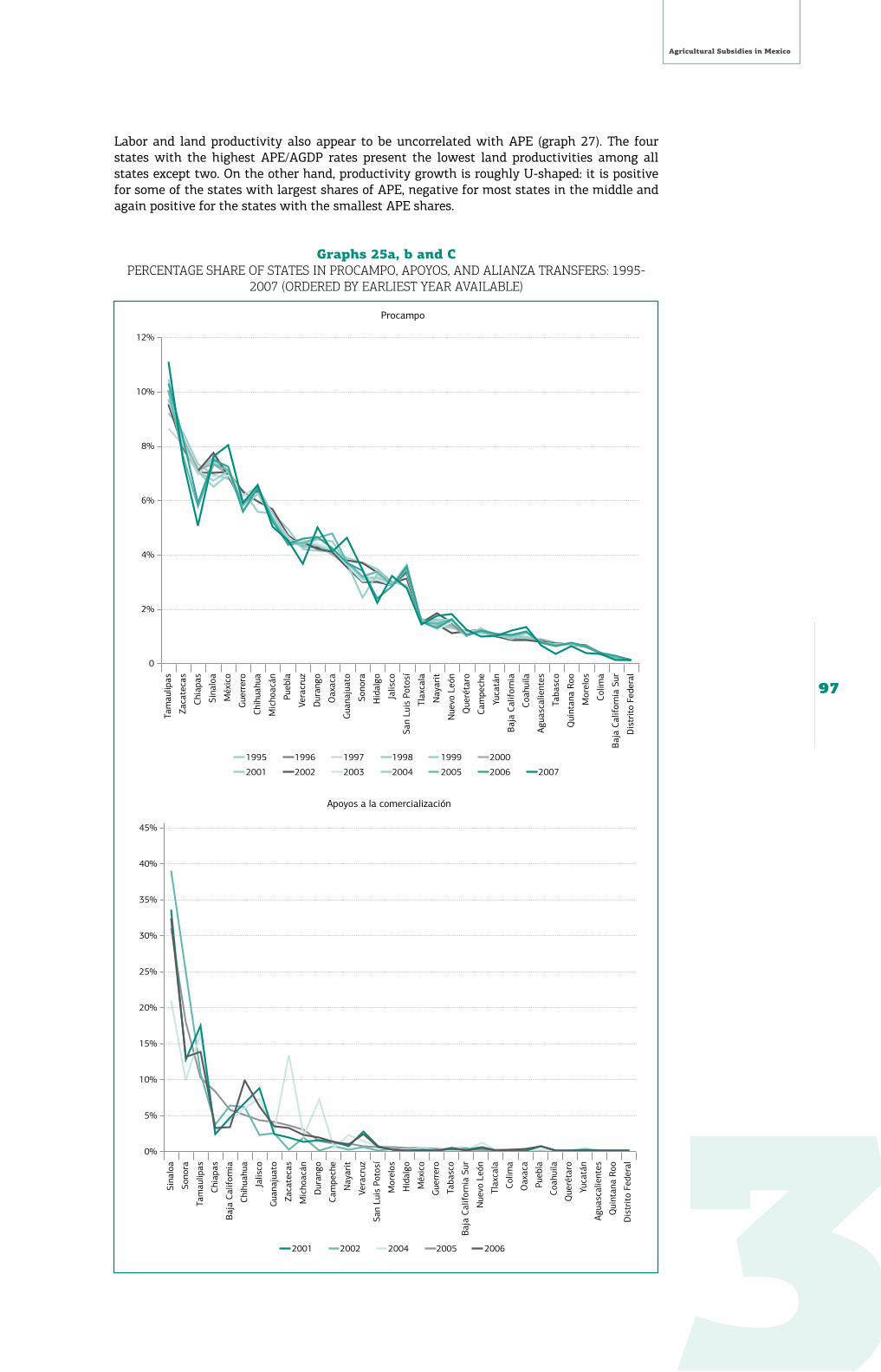
3
Agricultural Subsidies in Mexico
97
Labor and land productivity also appear to be uncorrelated with APE (graph 27). The four states with the highest APE/AGDP rates present the lowest land productivities among all states except two. On the other hand, productivity growth is roughly U-shaped: it is positive for some of the states with largest shares of APE, negative for most states in the middle and again positive for the states with the smallest APE shares.
Graphs 25a, b and CPercentAGe shAre of stAtes in ProcAmPo, APoyos, AnD AliAnzA trAnsfers: 1995-
2007 (orDereD by eArliest yeAr AvAilAble)
1995 1996 1997 1998 1999 2000
2001 2002 2003 2004 2005 2006 2007
Tam
aulip
as
Zaca
teca
s
Chia
pas
Sina
loa
Méx
ico
Gue
rrer
o
Chih
uahu
a
Mic
hoac
án
Pueb
la
Vera
cruz
Dur
ango
Oax
aca
Gua
naju
ato
Sono
ra
Hid
algo
Jalis
co
San
Luis
Pot
osí
Tlax
cala
Nay
arit
Nue
vo L
eón
Que
réta
ro
Cam
pech
e
Yuca
tán
Baj
a Ca
lifor
nia
Coah
uila
Agua
scal
ient
es
Taba
sco
Qui
ntan
a Ro
o
Mor
elos
Colim
a
Baj
a Ca
lifor
nia
Sur
Dis
trit
o Fe
dera
l
0
2%
4%
6%
8%
10%
12%
Procampo
2001 2002 2004 2005 2006
Sina
loa
Sono
ra
Tam
aulip
as
Chia
pas
Baj
a Ca
lifor
nia
Chih
uahu
a
Jalis
co
Gua
naju
ato
Zaca
teca
s
Mic
hoac
án
Dur
ango
Cam
pech
e
Nay
arit
Vera
cruz
San
Luis
Pot
osí
Mor
elos
Hid
algo
Méx
ico
Gue
rrer
o
Taba
sco
Baj
a Ca
lifor
nia
Sur
Nue
vo L
eón
Tlax
cala
Colim
a
Oax
aca
Pueb
la
Coah
uila
Que
réta
ro
Yuca
tán
Agua
scal
ient
es
Qui
ntan
a Ro
o
Dis
trit
o Fe
dera
l
0%
45%
35%
30%
40%
25%
20%
15%
10%
5%
Apoyos a la comercialización
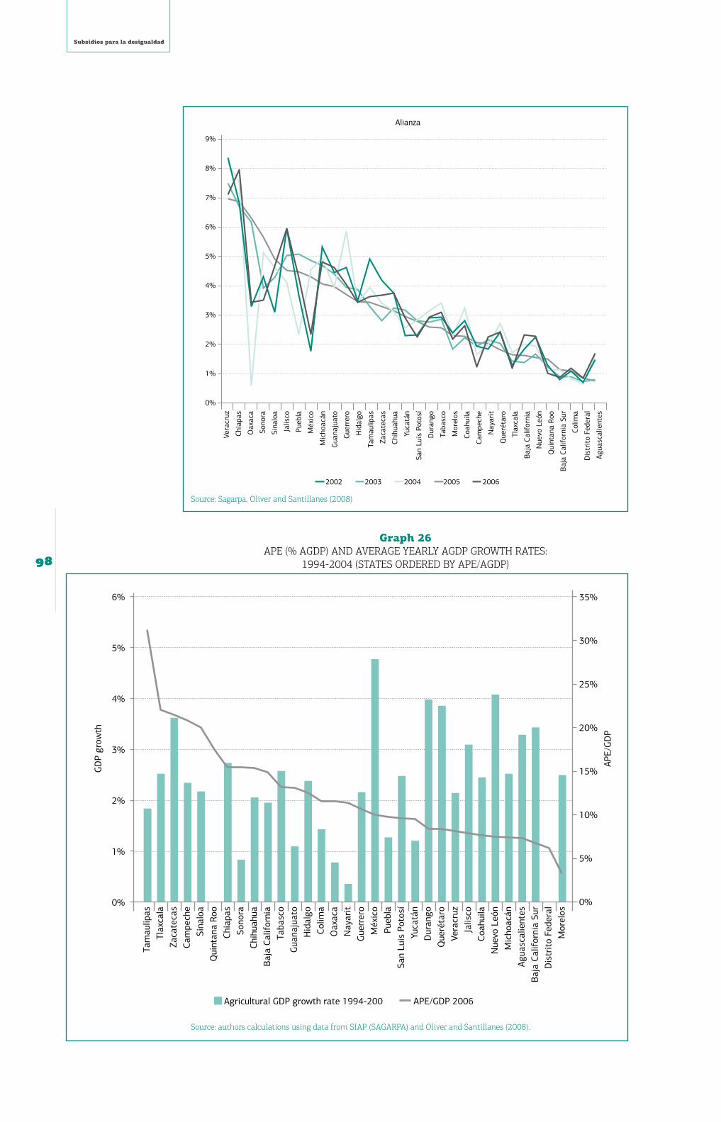
Subsidios para la desigualdad
98
source: sagarpa, oliver and santillanes (2008)
Graph 26APe (% AGDP) AnD AverAGe yeArly AGDP Growth rAtes:
1994-2004 (stAtes orDereD by APe/AGDP)
source: authors calculations using data from siAP (sAGArPA) and oliver and santillanes (2008).
2002 2003 2004 2005 2006
Vera
cruz
Chia
pas
Oax
aca
Sono
ra
Sina
loa
Jalis
co
Pueb
la
Méx
ico
Mic
hoac
án
Gua
naju
ato
Gue
rrer
o
Hid
algo
Tam
aulip
as
Zaca
teca
s
Chih
uahu
a
Yuca
tán
San
Luis
Pot
osí
Dur
ango
Taba
sco
Mor
elos
Coah
uila
Cam
pech
e
Nay
arit
Que
réta
ro
Tlax
cala
Baj
a Ca
lifor
nia
Nue
vo L
eón
Qui
ntan
a Ro
o
Baj
a Ca
lifor
nia
Sur
Colim
a
Dis
trit
o Fe
dera
l
Agua
scal
ient
es
0%
9%
7%
6%
8%
5%
4%
3%
2%
1%
Alianza
35%
30%
25%
20%
15%
10%
5%
0%0%
1%
2%
3%
4%
5%
6%
Tam
aulip
asTl
axca
laZa
cate
cas
Cam
pech
eSi
nalo
aQ
uint
ana
Roo
Chia
pas
Sono
raCh
ihua
hua
Baj
a Ca
lifor
nia
Taba
sco
Gua
naju
ato
Hid
algo
Colim
aO
axac
aN
ayar
itG
uerr
ero
Méx
ico
Pueb
laSa
n Lu
is P
otos
íYu
catá
nD
uran
goQ
ueré
taro
Vera
cruz
Jalis
coCo
ahui
laN
uevo
Leó
nM
icho
acán
Agua
scal
ient
esB
aja
Calif
orni
a Su
rD
istr
ito
Fede
ral
Mor
elos
Agricultural GDP growth rate 1994-200 APE/GDP 2006
GD
P gr
owth
APE/
GD
P
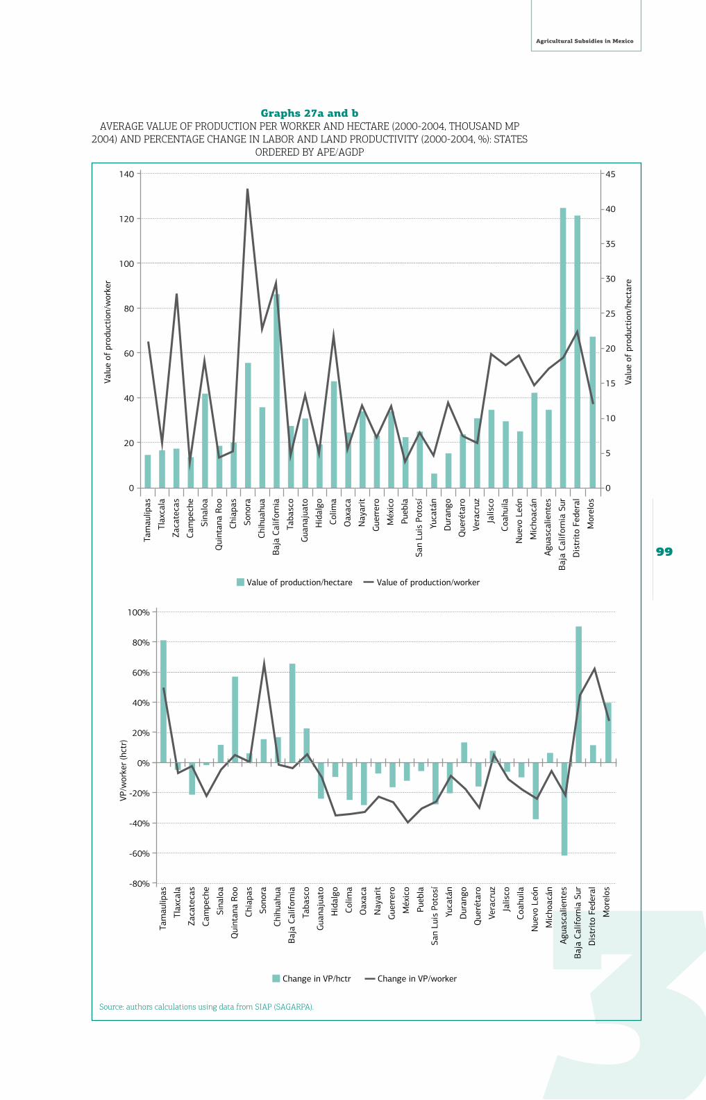
3
Agricultural Subsidies in Mexico
99
Graphs 27a and bAverAGe vAlue of ProDuction Per worker AnD hectAre (2000-2004, thousAnD mP
2004) AnD PercentAGe chAnGe in lAbor AnD lAnD ProDuctivity (2000-2004, %): stAtes orDereD by APe/AGDP
source: authors calculations using data from siAP (sAGArPA).
Value of production/hectare Value of production/worker
Tam
aulip
as
Tlax
cala
Zaca
teca
s
Cam
pech
e
Sina
loa
Qui
ntan
a Ro
o
Chia
pas
Sono
ra
Chih
uahu
a
Baj
a Ca
lifor
nia
Taba
sco
Gua
naju
ato
Hid
algo
Colim
a
Oax
aca
Nay
arit
Gue
rrer
o
Méx
ico
Pueb
la
San
Luis
Pot
osí
Yuca
tán
Dur
ango
Que
réta
ro
Vera
cruz
Jalis
co
Coah
uila
Nue
vo L
eón
Mic
hoac
án
Agua
scal
ient
es
Baj
a Ca
lifor
nia
Sur
Dis
trit
o Fe
dera
l
Mor
elos
Valu
e of
pro
duct
ion/
wor
ker
Valu
e of
pro
duct
ion/
hect
are
100
140
120
80
60
40
20
30
25
45
40
35
20
15
10
5
0 0
Change in VP/hctr Change in VP/worker
Tam
aulip
as
Tlax
cala
Zaca
teca
s
Cam
pech
e
Sina
loa
Qui
ntan
a Ro
o
Chia
pas
Sono
ra
Chih
uahu
a
Baj
a Ca
lifor
nia
Taba
sco
Gua
naju
ato
Hid
algo
Colim
a
Oax
aca
Nay
arit
Gue
rrer
o
Méx
ico
Pueb
la
San
Luis
Pot
osí
Yuca
tán
Dur
ango
Que
réta
ro
Vera
cruz
Jalis
co
Coah
uila
Nue
vo L
eón
Mic
hoac
án
Agua
scal
ient
es
Baj
a Ca
lifor
nia
Sur
Dis
trit
o Fe
dera
l
Mor
elos
VP/w
orke
r (h
ctr)
60%
100%
80%
40%
20%
0%
-40%
-60%
-20%
-80%

Subsidios para la desigualdad
100
Finally, graph 28 compares the distribution of employment loss in agriculture over the last decade (1996-2008) with the distribution of the principal support programs, ordering states by their share in the total employment loss over the period. Again, we observe a negative cor-relation: the states with the steepest agricultural employment losses receive on average more support.
These results may seem counterintuitive, but can be explained by several factors. First, APE and infrastructural investments have been concentrated historically in the largest and most developed agricultural states, where additional growth potential and productivity gains may thus be smaller than in the less developed states where public investment has been scarcer. Secondly, as noted before, a large proportion of agricultural subsidies is directed at large-scale and capital-intensive maize and other grain production, with limited direct employment po-tential. Finally, the results may also reflect a limited productive impact of most agricultural subsidies at the farm level. Many of these subsidies represent compensatory transfers rather than productivity-increasing investments, and for the latter impact evaluations are available for any of these programs.
Finally, to obtain a preliminary sense of the correlation between Procampo transfers and mi-gration decisions, we compare the distribution of Procampo beneficiaries at the municipality level with various census-based migration measures, including households receiving remit-tances (2000), households with migrants (2000), international migrants in 1995 and 2000, and the change in migrants between these two years (graph 35). This reveals a weak relation-ship between the distribution of Procampo and migration at the municipal level, at least in the case of poorer municipalities, as Procampo beneficiaries (in contrast to its transfers) are con-centrated disproportionately in the poorer municipalities, while migrants come disproportion-ately from municipalities with lower poverty levels. This is consistent with the results of a careful econometric analysis on this issue in a companion paper to the present study (Cuecue-cha and Scott 2010).
Graph 28AGriculturAl emPloyment AnD AGriculturAl subsiDies
source: author’s calculations based on data from enoe and oliver and santillanes (2008).
Share in national employment loss Agricultural employment loss 1996-2008
Procampo share (1995-2007) Other ASERCA share (2001-2006)
Alianza share (2002-2006)
Méx
ico
Jalis
co
Mic
hoac
án
Oax
aca
Vera
cruz
Gue
rrer
o
Chia
pas
Gua
naju
ato
Hid
algo
Sono
ra
Taba
sco
Nue
vo L
eón
Chih
uahu
a
Tam
aulip
as
Zaca
teca
s
Sina
loa
Que
réta
ro
Coah
uila
Dur
ango
Agua
scal
ient
es
Tlax
cala
Nay
arit
Cam
pech
e
Pueb
la
Baj
a Ca
lifor
nia
Sur
Yuca
tán
San
Luis
Pot
osí
Colim
a
Qui
ntan
a Ro
o
Baj
a Ca
lifor
nia
Mor
elos
Shar
e, c
hang
e in
agr
icul
tura
l em
ploy
men
t 0%
20%
10%
-10%
-20%
-30%
-50%
-60%
-40%
-70%
Proc
ampo
, ASE
RCA,
Alia
nza
35%
30%
25%
20%
15%
10%
5%
0%

3
Agricultural Subsidies in Mexico
101
Box7:does ProcamPo lImIt mIgratIon to tHe us?AlfredoCuechuechaandJohnScott(CIDE)
While rural citizens’ decisions to leave the countryside are influenced by many factors, the availability of agricultural employment is certainly one of them. In principle, farm subsidies that are large enough to make agricultural production by small and medium-sized farmers economically viable should have the effect of discouraging migration, not only by the producers themselves, but also by those who they might employ locally. Re-search strategies included both analysis of the impact on local labor markets (at the municipal level), as well as household and individual level impacts, based on National Employment Survey 2005-2006 data (ENOE).
The study of local labor market impacts found that the increase in migration levels was highest where Procampo payments were lowest. At higher levels of Procampo payments, in contrast, there is a positive relationship with increases in municipal migration levels, which suggests the need for additional research. The study of individual and household responses allows for greater precision, and the econometric analysis focused on the effect of each additional peso of Procampo payments on migration flows at the family level (while holding many relevant variables constant). This analysis found that Procampo payments were associated with statistically significant, though modest reductions in migration levels. Procampo was also associated with retaining employment in the corn and bean sectors, and negatively associated with employment in fruits and vegetables.
Note: This box summaries the extensive findings presented in Alfredo Cuecuecha and John Scott, “The effect of agricultural subsidies on migration and agricultural employ-ment,” Woodrow Wilson Center, Mexico Institute, Rural Development Research Report, No. 3., January, 2010
Graph 29municiPAl ProcAmPo AnD miGrAtion concentrAtion curves: 1995-2000
source: author’s calculations using AsercA administrative data, conevAl municipal poverty measures, and 1995 conteo
and 2000 censo de Población y vivienda (ineGi).
0
0.1
0.2
0.3
0.4
0.5
0.6
0.7
0.8
0.9
1
0.04
0.07
0.09
0.12
0.14
0.16 0.2
0.23
0.25
0.29
0.32
0.35
0.38
0.41
0.43
0.46
0.49
0.52
0.55
0.57 0.6
0.63
0.67 0.7
0.73
0.75
0.78
0.81
0.83
0.86
0.89
0.92
0.94
0.97
Rural poverty (alimentaria) Procampo beneficiaries 2000 Procampo transfers 2000
Households with migrants 2000 Households receiving remittances 2000 Migrants 1995-2000
Migrants 2000 Migrants 1995
Subsidios para la desigualdad
102
6. dIstrIbutIon oF agrIcultural andrural develoPment Programs among HouseHolds and ProducersIn this section the distribution of benefits is analyzed at the level of individual producers and households. The availability of household and producer data bases reporting both agricultural support programs and a relevant measure of household/producer wellbeing or wealth is lim-ited. This study uses three kinds of data sources, which are complementary but not strictly comparable: a) national household surveys including coverage of ARD programs (ENIGH 2006 and 2008, and ENIGH-Modulo Social 2006), b) evaluation surveys for specific programs (Alian-za, Oportunidades), and c) administrative data of the programs (Procampo, Ingreso Objetivo). The national household surveys have the important advantages of being nationally represen-tative and including high-quality data on income and other measures of welfare, but their sample size is not designed to capture specific transfer programs accurately, especially when these have limited coverage or concentrate a large share of their benefits in a relatively small proportion households. The other two sources are designed to capture the program beneficia-ries and transfers accurately, but are not nationally representative and generally contain lim-ited or no income data. The analysis obtained from the three sources must therefore be inter-preted carefully and complementarily.
The distribution of benefits is analyzed using two different ordering criteria corresponding to the alternative data sources. In the case of administrative data, producers are ordered by land holdings, which is the only proxy of wealth/welfare available in this data. In the case of the national household surveys, benefits received are analyzed by population deciles ordered by total current income per capita.
DataSourcesData Source Program
ENIGH 2006, 2008 Procampo, Oportunidades
ENIGH-Modulo Social 2006 Social and rural development programs
Oportunidades recertification and identification data base (ENCASEH 2004)
Oportunidades, Procampo
ASERCA beneficiary data base (2005, 2006) Procampo, Ingreso Objetivo
Alianza evaluation data base – Evalianza (2005, 2006), FAO-Sagarpa
Alianza para el Campo
The household and producer data available allows coverage of the principal ARD programs, including the principal agricultural support programs (Procampo, Ingreso Objetivo, and Alian-za), as well as the principal rural social programs, including Oportunidades, Adultos Mayores 70 y más, and Programa de Empleo Temporal. We also estimate the distribution of hydro-agri-cultural and agricultural electricity subsidies (Tarifa 9) using the distribution of irrigated land as a (rough) proxy. The agricultural support programs covered in this incidence analysis repre-sent approximately 75% of total APE in Mexico.
6.1Resourcedistributionpatternsamongproducers,bydecile,orderedbyland-holdings
Before analyzing the distribution of agricultural subsidies by producer deciles (ranked by land-hold-ings), we consider the distribution of producers grouped by average size of land-holdings. Us-ing administrative data, producers with less than 5 has represent 75% of Procampo´s beneficiaries, but receive 37% of the program’s transfers, reflecting their share in covered land (graph 30). Producers with 5-20 has represent 22% of beneficiaries and receive 41% of the benefits, while pro-ducers with more than 20 has represent 3% of the beneficiaries and obtain 23% of the transfers.
Is all the regressivity of Procampo explained by the distribution of land in Mexico, or is the program’s coverage of producers also biased against smaller producers? Comparison between the Procampo data and the 2007 Agricultural Census in the aggregate suggest no such bias, neither at the state level (see graph 21a) nor at the national level (graph 5, above): coverage is highest among small 0-5 (66%) and medium (63%) producers. However, the evidence from poor rural localities presents a somewhat different picture (graph 31), with coverage declining with land size, to just 19% for 1-2 has and 7% for less than 1 ha. This issue requires further investigation. One possible explanation for the difference between the two sources might be that the Census might under-report smaller producer units.

3
Agricultural Subsidies in Mexico
103
Graph 30Distribution of ProDucers AnD trAnsfers from ProcAmPo AnD inGreso objetivo
between ProcAmPo beneficiAries (2006)
source: author’s calculations using AsercA administrative data.
Graph 31coverAGe of oPortuniDADes AnD ProcAmPo AmonG householDs in Poor rurAl
locAlities, by size of lAnD owneD or useD (2004).
source: author’s calculations encAseh 2004 oportunidades survey.
0
10
20
30
40
50
60
0-2 2-5 5-10 10-20 20-100
Producers Procampo transfers Ingreso Objetivo transfers
32%
43%
28%
8%
16%
24%
13%
6%
17%
22%
3%
23%
57%
9%
1%
0
10
20
30
40
50
60
Procampo Oportunidades Both Neither
Land
less
, non
agri
cultu
ral
<1 H
A
1-2H
A
2-5H
A
6-10
HA
11-2
0HA
20+H
A
Land
less
, ag
ricu
ltura
l
50%
0% 0% 0%
44%
7%
46%
4%
19%
58%
39%
56%
23%
47%
51%
44%
35%
19%
42%
38%
16%
28%
11%
1%
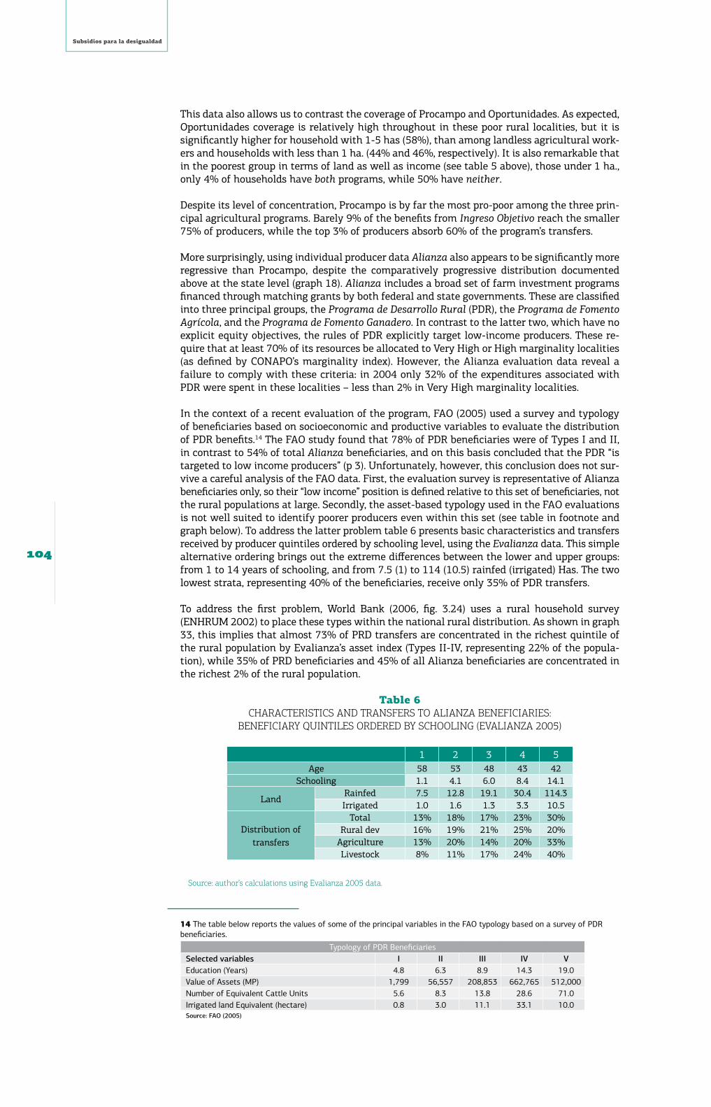
Subsidios para la desigualdad
104
This data also allows us to contrast the coverage of Procampo and Oportunidades. As expected, Oportunidades coverage is relatively high throughout in these poor rural localities, but it is significantly higher for household with 1-5 has (58%), than among landless agricultural work-ers and households with less than 1 ha. (44% and 46%, respectively). It is also remarkable that in the poorest group in terms of land as well as income (see table 5 above), those under 1 ha., only 4% of households have both programs, while 50% have neither.
Despite its level of concentration, Procampo is by far the most pro-poor among the three prin-cipal agricultural programs. Barely 9% of the benefits from Ingreso Objetivo reach the smaller 75% of producers, while the top 3% of producers absorb 60% of the program’s transfers.
More surprisingly, using individual producer data Alianza also appears to be significantly more regressive than Procampo, despite the comparatively progressive distribution documented above at the state level (graph 18). Alianza includes a broad set of farm investment programs financed through matching grants by both federal and state governments. These are classified into three principal groups, the Programa de Desarrollo Rural (PDR), the Programa de Fomento Agrícola, and the Programa de Fomento Ganadero. In contrast to the latter two, which have no explicit equity objectives, the rules of PDR explicitly target low-income producers. These re-quire that at least 70% of its resources be allocated to Very High or High marginality localities (as defined by CONAPO’s marginality index). However, the Alianza evaluation data reveal a failure to comply with these criteria: in 2004 only 32% of the expenditures associated with PDR were spent in these localities – less than 2% in Very High marginality localities.
In the context of a recent evaluation of the program, FAO (2005) used a survey and typology of beneficiaries based on socioeconomic and productive variables to evaluate the distribution of PDR benefits.14 The FAO study found that 78% of PDR beneficiaries were of Types I and II, in contrast to 54% of total Alianza beneficiaries, and on this basis concluded that the PDR “is targeted to low income producers” (p 3). Unfortunately, however, this conclusion does not sur-vive a careful analysis of the FAO data. First, the evaluation survey is representative of Alianza beneficiaries only, so their “low income” position is defined relative to this set of beneficiaries, not the rural populations at large. Secondly, the asset-based typology used in the FAO evaluations is not well suited to identify poorer producers even within this set (see table in foo tnote and graph below). To address the latter problem table 6 presents basic characteristics and transfers received by producer quintiles ordered by schooling level, using the Evalianza data. This simple alternative ordering brings out the extreme differences between the lower and upper groups: from 1 to 14 years of schooling, and from 7.5 (1) to 114 (10.5) rainfed (irrigated) Has. The two lowest strata, representing 40% of the beneficiaries, receive only 35% of PDR transfers.
To address the first problem, World Bank (2006, fig. 3.24) uses a rural household survey (ENHRUM 2002) to place these types within the national rural distribution. As shown in graph 33, this implies that almost 73% of PRD transfers are concentrated in the richest quintile of the rural population by Evalianza’s asset index (Types II-IV, representing 22% of the popula-tion), while 35% of PRD beneficiaries and 45% of all Alianza beneficiaries are concentrated in the richest 2% of the rural population.
Table 6chArActeristics AnD trAnsfers to AliAnzA beneficiAries:
beneficiAry quintiles orDereD by schoolinG (evAliAnzA 2005)
1 2 3 4 5Age 58 53 48 43 42
Schooling 1.1 4.1 6.0 8.4 14.1
LandRainfed 7.5 12.8 19.1 30.4 114.3Irrigated 1.0 1.6 1.3 3.3 10.5
Distribution of transfers
Total 13% 18% 17% 23% 30%Rural dev 16% 19% 21% 25% 20%
Agriculture 13% 20% 14% 20% 33%Livestock 8% 11% 17% 24% 40%
source: author’s calculations using evalianza 2005 data.
14 The table below reports the values of some of the principal variables in the FAO typology based on a survey of PDR beneficiaries.
Typology of PDR BeneficiariesSelected variables I II III IV VEducation (Years) 4.8 6.3 8.9 14.3 19.0Value of Assets (MP) 1,799 56,557 208,853 662,765 512,000Number of Equivalent Cattle Units 5.6 8.3 13.8 28.6 71.0Irrigated land Equivalent (hectare) 0.8 3.0 11.1 33.1 10.0Source: FAO (2005)
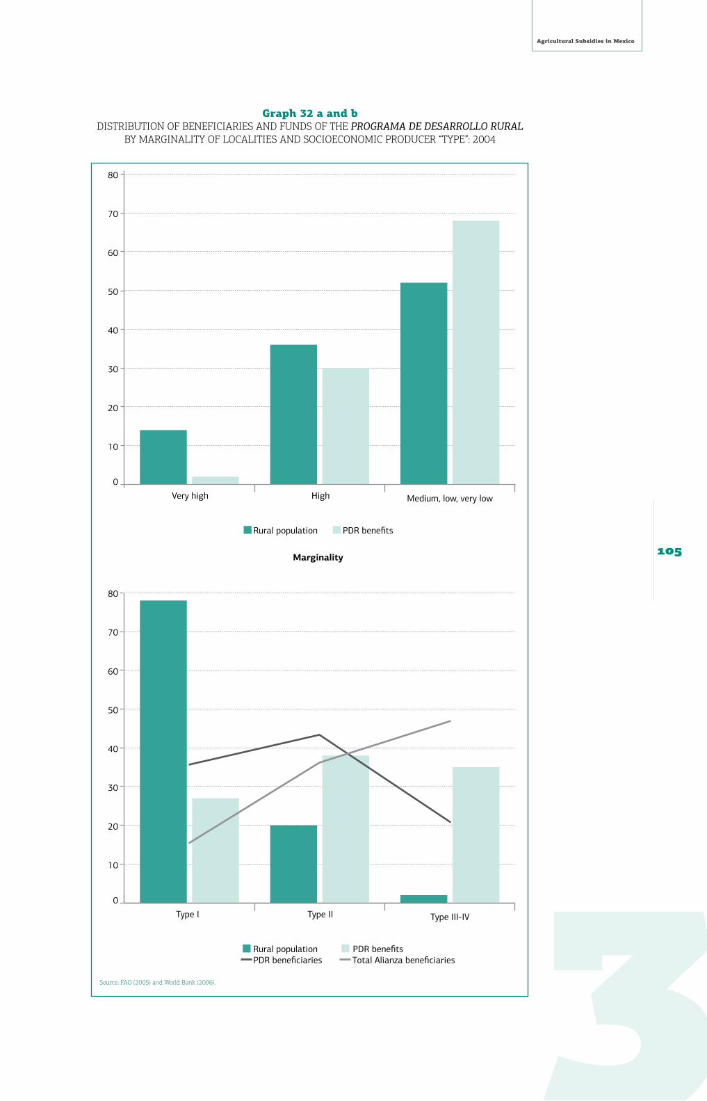
3
Agricultural Subsidies in Mexico
105
Graph 32 a and bDistribution of beneficiAries AnD funDs of the PROGRAMA DE DESARROLLO RuRAL
by mArGinAlity of locAlities AnD socioeconomic ProDucer “tyPe”: 2004
source: fAo (2005) and world bank (2006).
0
10
20
30
40
50
60
70
80
Rural population PDR benefits
Medium, low, very lowVery high High
Marginality
0
10
20
30
40
50
60
70
80
Rural population PDR benefitsPDR beneficiaries Total Alianza beneficiaries
Type III-IVType I Type II

Subsidios para la desigualdad
106
To compare the distribution of the principal APE programs on a common basis we present the distribution of benefits by producer deciles, and concentration curves based on producer per-centiles, ranking producers by two alternative land measures:
(1) size of land holdings as reported in the administrative or evaluation data, and (2) quality-adjusted land assets: as a more accurate proxy for producer income and wealth an approximation to the value of land assets obtained from the estimated value of production in each productive unit taking into account a) whether it is rainfed or irrigated, b) crop type, c) size of cultivated land, and d) average productivity and prices by State (using Sagarpa data).
Table 7 presents the distribution of Procampo and Ingreso Objetivo using the two concepts, and graphs 34-36 present concentration curves for these programs, for Alianza (fitted from the observations available from the FAO data presented above) and for energy and hydro-agricul-tural subsidies (proxied by the distribution of irrigated land). This analysis reveals extreme concentrations of benefits for all programs, except for Procampo in the quality-adjusted rank-ings. The poorest producer decile (in terms of both rankings) receives a tenth of a percentage point of Ingreso Objetivo, similarly insignificant fractions of energy/irrigation subsidies, and only 2-3% of Procampo. At the other extreme, the producers in the top decile receive transfer shares in the order of:
42% (33%) of Procampo (adjusted) 55% of the Alianza PDR, 60% of energy and hydrological subsidies, 85% (90%) of Ingreso Objetivo.
These distributions are of course mutually reinforcing. In addition to the large subsidies as-sociated with irrigation, as graph 43 shows, the distribution of Procampo and Ingreso Objetivo are more regressive for irrigated than for rain-fed land.
It is interesting that the more accurate measure of producer wealth reduces the degree of re-gressivity in the case of Procampo but it increases it in Ingreso Objetivo. This suggests that many of the larger beneficiaries from Procampo given the size of their lands may be poorer once the land is adjusted for quality (and viceversa for smaller ones), while Ingreso Objetivo is not only concentrated on larger land-holdings but also on those with the more productive ones.
Table 7Distribution of ProcAmPo AnD inGreso objetivo trAnsfers by ProDucer Deciles
rAnkeD by (1) lAnD holDinGs AnD (2) quAlity-ADjusteD lAnD holDinGs(sPrinG-summer 2006)
Producer Deciles
Land (Has) Distribution of transfers
AverageRange Procampo Ingreso Objetivo
Min Max (1) (2) (1) (2)
1 0.93 0.01 1.00 2.2% 2.9% 0.1% 0.1%
2 1.00 1.00 1.00 2.3% 3.4% 0.1% 0.3%
3 1.39 1.00 1.75 3.2% 3.9% 0.3% 0.0%
4 1.98 1.75 2.00 4.6% 5.1% 1.0% 0.2%
5 2.12 2.00 2.50 4.9% 6.4% 2.6% 0.2%
6 2.90 2.50 3.00 6.7% 7.6% 1.4% 0.9%
7 3.62 3.00 4.00 8.3% 9.9% 2.0% 0.8%
8 4.75 4.00 5.79 10.8% 12.1% 2.6% 1.3%
9 6.99 5.79 9.00 15.2% 15.8% 5.0% 6.8%
10 20.48 9.00 1957.5 41.8% 33.0% 85.0% 89.6%
Percentiles
90-97 9 20 17% 23%
98-100 20 1957.5 25% 62%
source: author’s calculations using AsercA administrative data.

3
Agricultural Subsidies in Mexico
107
Graph 33 ProcAmPo, inGreso objetivo, AliAnzA (DesArrollo rurAl), AnD lAnD
concentrAtion curves: orDereD by Plot size
source: author’s calculations using AsercA administrative data, fAo (2005) and world bank (2006).
Graph 34ProcAmPo AnD inGreso objetivo concentrAtion curves:
rAinfeD AnD irriGAteD lAnD
source: author’s calculations using AsercA administrative data.
Procampo Ingreso Objetivo Alianza-Desarrollo rural Irrigated Land Rainfed Land
0
10%
20%
30%
40%
50%
60%
70%
80%
90%
100%
10% 20% 30% 40% 50% 60% 70% 80% 90% 100%
0
10%
20%
30%
40%
50%
60%
70%
80%
90%
100%
10% 20% 30% 40% 50% 60% 70% 80% 90% 100%
Irrigated Land Rainfed Land Procampo (irrigated) Ingreso Objetivo (irrigated)
Procampo (rainfed) Ingreso Objetivo (rainfed)

Subsidios para la desigualdad
108
Graph 35ProcAmPo, inGreso objetivo AnD lAnD:
orDereD by estimAteD lAnD vAlue/ProDucer income
source: author’s calculations using AsercA administrative data, fAo (2005) and world bank (2006).
6.2.Resourcedistributionamonghouseholds,bydecilesorderedbyincomepercapita
To put these distributions in the context of public rural spending on social programs as well as the national and rural income distribution, and to estimate the distributive impact of these resources, in this section we analyze the distribution of Procampo and the principal social programs using the ENIGH 2006 survey (and its associated “Modulo de Programas Sociales”). In the case of Procampo, the only agricultural program reported in this survey, these results must be interpreted with some care, as the survey is not designed to be representative of in-dividual transfers, especially when a large proportion of their resources is concentrated on a small fraction of the population in the top decile, as we have just seen is the case of Procam-po.15 Despite this, the ENIGH data confirm a concentration of benefits in the top decile (graph 36), where 4.5% of Procampo’s beneficiaries receive 27% of the program’s transfers, while the poorest income decile accounts for 20% of beneficiaries but 8.7% of benefits.
The contrast between the principal social and agricultural programs, Oportunidades and Pro-campo, is evident from their concentration curves in income space, both nationally and with-in the rural sector (graph 37).
A critical issue in this analysis is the position of the APE concentration curves with respect to the (pre-transfer) income Lorenz curve, as this determines whether these programs are simply ineffective as redistributive instruments, or actually contribute to increase income inequality (below the Lorenz curve). The noted data limitations in both the ENIGH and the administrative data preclude a direct and unambiguous settlement of the issue. It seems reasonable to con-
15 The analysis above based on administrative data has shown that a quarter of the program transfers are received by the top 3% of producers. As is well known the ENIGH survey does not capture HH incomes at the upper extreme of the income distribution very well, for three principal reasons: a) the low statistical probability of selecting this small set of HHs in the sample, b) these HHs are less likely to participate once selected, an c) even if they are selected and agree to participate, they are more likely to underreport their income. The sizable measured underreporting of aggregate incomes and spending in the ENIGH in relation to the National Accounts is attributed in part to this truncation, and is the principal reason why the official methodology to measure poverty in Mexico does not adjust income to National Accounts. See Leyva-Parra (2005) and Scott (2005). This seems to be the main explanation for the large difference in the degree of estimated regressivity for Procampo using ENIGH (0.12) vs. administrative data (0.50).
Income (Enigh 2008) Procampo adjusted PV Land Land, adjusted Ingreso Objetivo, adjusted PV
0
10%
20%
30%
40%
50%
60%
70%
80%
90%
100%
10% 20% 30% 40% 50% 60% 70% 80% 90% 100%

3
Agricultural Subsidies in Mexico
109
clude that Procampo (and perhaps Alianza’s PDR) is probably progressive in relative terms: its concentration curve is well above the income Lorenz curve generated by the ENIGH data (graph 37), but similar to the latter when using administrative data (graph 35, 38).
Graph 36Distribution of ProcAmPo beneficiAries AnD trAnsfers by nAtionAl PoPulAtion
Deciles (orDereD by Pre-trAnsfer income Per cAPitA): 2006
source: author’s calculations using eniGh 2006.
But Procampo is probably the exception among (non-targeted) agricultural subsides. The con-centration curve for agricultural land and perhaps even quality-adjusted land may reasonably be interpreted as an upper bound for the concentration curves of non-targeted, input- or out-put-linked transfers and subsidies, generally: a large part of the rural population (at least the poorest 50%) is excluded from such programs simply because they are either landless or have plots which are too small to be reached by such programs (except for a decoupled program like Procampo), and in the upper half of the land distribution there are probably strong economies of scale (and land quality) in the capacity to attract agricultural support resources (unless some explicit targeting is applied, as in the case of the PDR). This applies clearly to the case of input support programs like the energy subsidies (diesel agropecuario and tarifa 9). This im-plies that the majority of agricultural support programs, and APE overall, are regressive in relative terms, and thus a contributing cause of rural income inequality.
These estimates of course only consider the direct, first-order incidence of the benefits from APE. In a general equilibrium setting, agricultural workers and small land owners may share some of the benefits from the agricultural support transfers obtained by large commercial producers, through higher wages and land prices. However, there are at least two reasons to doubt that such “trickle-down” effects would be sufficient to reverse the first-order effect. First, as we have seen, the large, grain-producing commercial farms in the northern states benefit-ing from these transfers tend to be capital- rather than labor-intensive. Secondly, by further increasing the cost-advantage of large-scale producers, these transfers undermine the capac-ity of small (potentially) commercial producers to compete in these markets. Note that the argument to support these smaller but viable farmers is exactly analogous to the argument often used in favor of supporting the larger commercial producers to compensate them for unfair competition due to international subsidies.
To compare the equity of APE more systematically in the context of RD expenditures, and as-sess the global impact of ARD expenditures on rural income inequality, we can compare the APE programs analyzed above with the social and rural development programs reported in the ENIGH 2006 and a special “Social Program Module” commissioned by Sedesol with the ENIGH 2006. The following graphs compare two synthetic indicators: concentration coefficients (CC) and the shares of transfers received by the poorest/richest quintile.
1 2 3 4 5 6 7 8 9 10
0%
5%
10%
15%
20%
25%
30%
Beneficiaries Tranfers
20.4%
8.7%
14.8%
8.7%
11.4%
7.1%
11.8%
7.1%
11.2%
8.2%8.9% 8.7%
5.3%
8.8%
5.6%
6.9%6.2%
8.9%
4.5%
27%
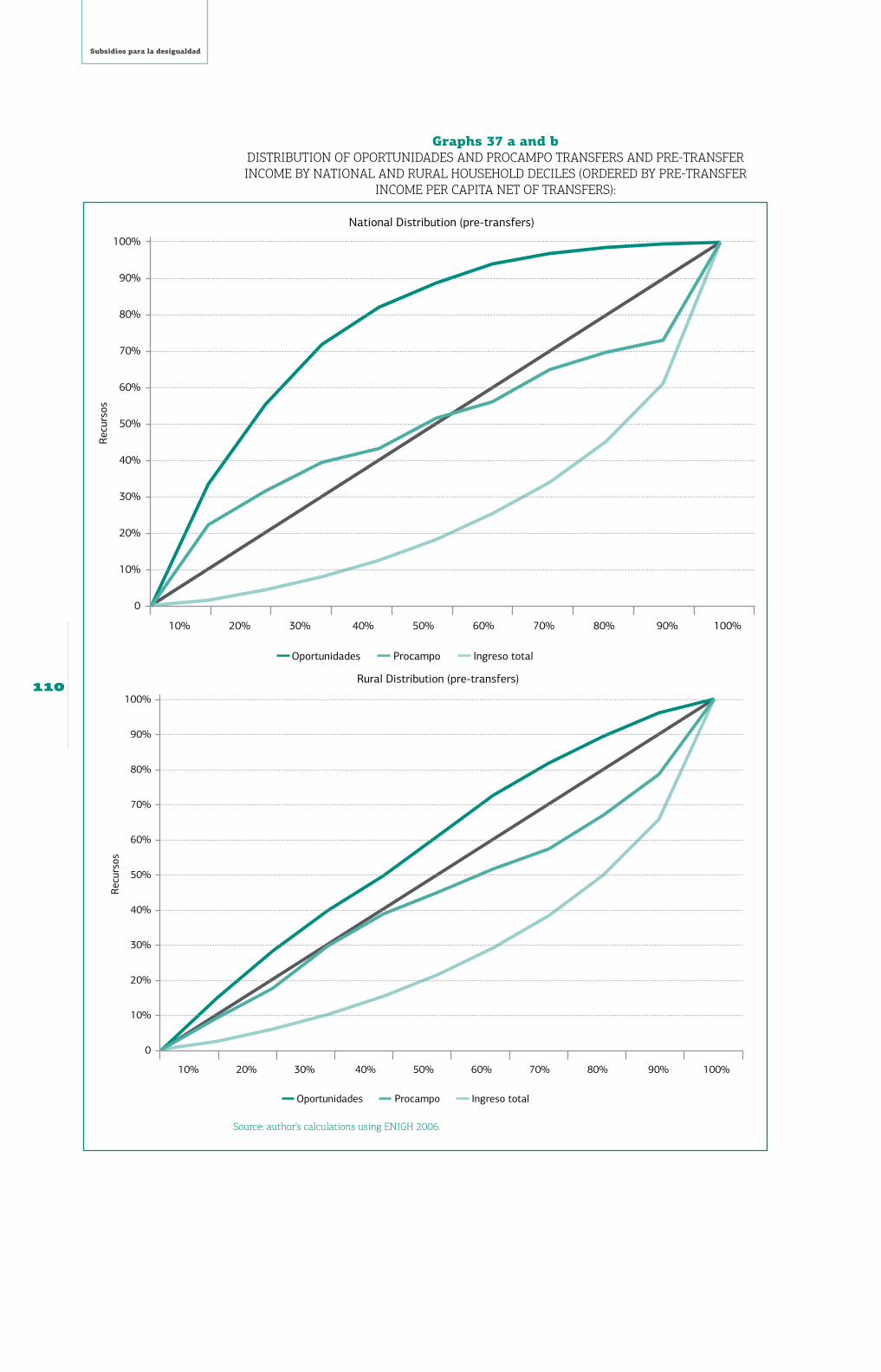
Subsidios para la desigualdad
110
Graphs 37 a and bDistribution of oPortuniDADes AnD ProcAmPo trAnsfers AnD Pre-trAnsferincome by nAtionAl AnD rurAl householD Deciles (orDereD by Pre-trAnsfer
income Per cAPitA net of trAnsfers):
source: author’s calculations using eniGh 2006.
Oportunidades Procampo Ingreso total
Recu
rsos
0
10%
20%
30%
40%
50%
60%
70%
80%
90%
100%
10% 20% 30% 40% 50% 60% 70% 80% 90% 100%
National Distribution (pre-transfers)
Oportunidades Procampo Ingreso total
Recu
rsos
0
10%
20%
30%
40%
50%
60%
70%
80%
90%
100%
10% 20% 30% 40% 50% 60% 70% 80% 90% 100%
Rural Distribution (pre-transfers)
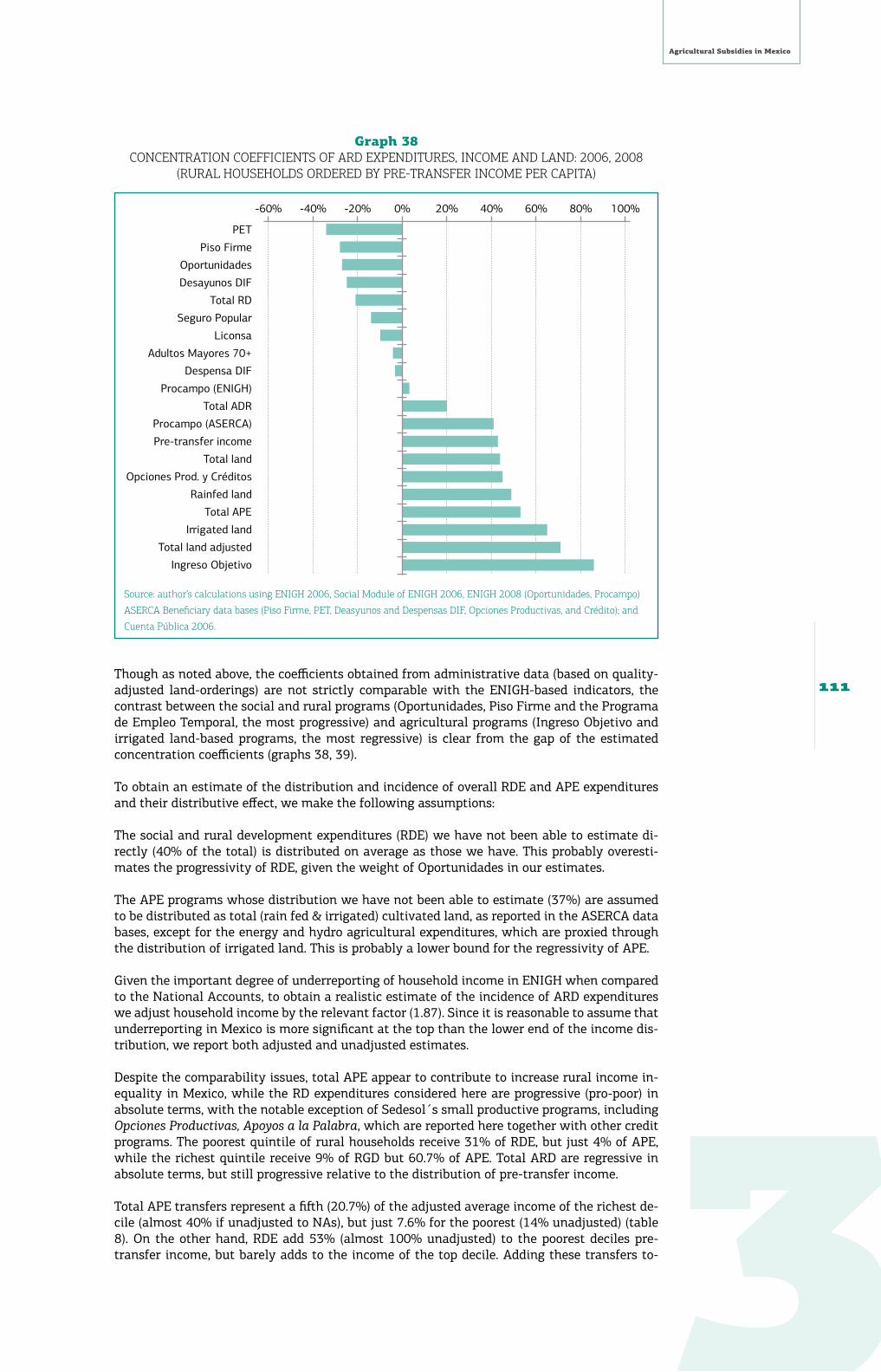
3
Agricultural Subsidies in Mexico
111
Graph 38concentrAtion coefficients of ArD exPenDitures, income AnD lAnD: 2006, 2008
(rurAl householDs orDereD by Pre-trAnsfer income Per cAPitA)
source: author’s calculations using eniGh 2006, social module of eniGh 2006, eniGh 2008 (oportunidades, Procampo)
AsercA beneficiary data bases (Piso firme, Pet, Deasyunos and Despensas Dif, opciones Productivas, and crédito); and
cuenta Pública 2006.
Though as noted above, the coefficients obtained from administrative data (based on quality-adjusted land-orderings) are not strictly comparable with the ENIGH-based indicators, the contrast between the social and rural programs (Oportunidades, Piso Firme and the Programa de Empleo Temporal, the most progressive) and agricultural programs (Ingreso Objetivo and irrigated land-based programs, the most regressive) is clear from the gap of the estimated concentration coefficients (graphs 38, 39).
To obtain an estimate of the distribution and incidence of overall RDE and APE expenditures and their distributive effect, we make the following assumptions:
The social and rural development expenditures (RDE) we have not been able to estimate di-rectly (40% of the total) is distributed on average as those we have. This probably overesti-mates the progressivity of RDE, given the weight of Oportunidades in our estimates.
The APE programs whose distribution we have not been able to estimate (37%) are assumed to be distributed as total (rain fed & irrigated) cultivated land, as reported in the ASERCA data bases, except for the energy and hydro agricultural expenditures, which are proxied through the distribution of irrigated land. This is probably a lower bound for the regressivity of APE.
Given the important degree of underreporting of household income in ENIGH when compared to the National Accounts, to obtain a realistic estimate of the incidence of ARD expenditures we adjust household income by the relevant factor (1.87). Since it is reasonable to assume that underreporting in Mexico is more significant at the top than the lower end of the income dis-tribution, we report both adjusted and unadjusted estimates.
Despite the comparability issues, total APE appear to contribute to increase rural income in-equality in Mexico, while the RD expenditures considered here are progressive (pro-poor) in absolute terms, with the notable exception of Sedesol´s small productive programs, including Opciones Productivas, Apoyos a la Palabra, which are reported here together with other credit programs. The poorest quintile of rural households receive 31% of RDE, but just 4% of APE, while the richest quintile receive 9% of RGD but 60.7% of APE. Total ARD are regressive in absolute terms, but still progressive relative to the distribution of pre-transfer income.
Total APE transfers represent a fifth (20.7%) of the adjusted average income of the richest de-cile (almost 40% if unadjusted to NAs), but just 7.6% for the poorest (14% unadjusted) (table 8). On the other hand, RDE add 53% (almost 100% unadjusted) to the poorest deciles pre-transfer income, but barely adds to the income of the top decile. Adding these transfers to-
PET
Piso Firme
Oportunidades
Desayunos DIF
Total RD
Seguro Popular
Liconsa
Adultos Mayores 70+
Despensa DIF
Procampo (ENIGH)
Total ADR
Procampo (ASERCA)
Pre-transfer income
Total land
Opciones Prod. y Créditos
Rainfed land
Total APE
Irrigated land
Total land adjusted
Ingreso Objetivo
0% 20% 40% 60%-60% -40% -20% 80% 100%

Subsidios para la desigualdad
112
gether, the distribution of public ARD expenditures is flat for the poorest 40%, at close to $400 pesos per capita per month, but increases sharply in the tenth decile, where rural households obtain on average more than $3000 pesos monthly per capita.
In purely accounting terms, APE increases the rural Gini coefficient by 6.7% (11.5% unadjust-ed), while RDE decreases it by 14% (24.8% unadjusted), with a net reduction of 6.5% associ-ated with total ARD. In other words, APE appears to cancel more than half of the redistribu-tive impact of RDE on relative inequality, measured through the Gini coefficient (though not, of course, on poverty reduction).
While the recognition and concern for the inequity of APE in Mexico has grown in recent years, partly as a result of the increasing availability of the type of evidence reviewed in this study, reform efforts to address these inequities have so far been timid and have clearly been effectively blocked by large producer interest groups and agricultural states. For example, fol-lowing the recommendations of a number of special advisory groups on Procampo reform set up by Sagarpa and the President’s Office, as well a the numerous national and international reports cited before, there was apparently a genuine intention on the part of the federal gov-ernment to limit Procampo transfers to small and medium-sized farmers, but this was effec-tively blocked by the noted interest groups. The result was a marginal reform of the Procampo rules which increased transfers to small (rainfed) farmers, while limiting maximum benefits per producer per cycle to 100,000 pesos. Graph 43 shows the results of a simulation of this reform applied to the ASERCA data base, revealing a negligible distributive impact.
A more recent reform effort is contained in the federal budget proposal for 2010, which pro-poses mayor cuts in perhaps the most regressive APE instrument of all, Ingreso Objetivo. It will be interesting to see if this proposal survives the legislative negotiation.
Graph 39relAtive shAre of Poorest 20% of rurAl householDs in of ArD exPenDitures,
income AnD lAnD: 2006, 2008 (rurAl householDs orDereDby Pre-trAnsfer income Per cAPitA)
source: author’s calculations using eniGh 2006, social module of eniGh 2006, eniGh 2008 (oportunidades, Procampo)
AsercA beneficiary data bases (Piso firme, Pet, Deasyunos and Despensas Dif, opciones Productivas, and crédito)..
Poorest 20% Richest 20%
0% 20% 40% 60% 80% 100%
PET
Piso Firme
Desayunos DIF
Oportunidades
Total RD
Adultos Mayores 70+
Procampo (ENIGH)
Seguro Popular
Despensa DIF
Total ADR
Liconsa
Opciones Prod. y Créditos
Procampo (ASERCA adjusted land)
Total land
Pre-transfer income
Rainfed land
Total APE
Irrigated land
Total land adjusted
Ingreso Objetivo

3
Agricultural Subsidies in Mexico
113
Graph 40Distribution of APe AnD rDe
(rurAl householD Deciles orDereD by income Per cAPitA before trAnsfers)
source: author’s calculations using eniGh 2006, social module of eniGh 2006, eniGh 2008 (oportunidades, Procampo)
AsercA beneficiary data bases (Piso firme, Pet, Deasyunos and Despensas Dif, opciones Productivas, and crédito); and
cuenta Pública 2006.
Graph 41inciDence of APe AnD rDe in rurAl householD income: trAnsfers
As % of Pre-trAnsfer income(householD Deciles orDereD by income Per cAPitA before trAnsfers)
source: author’s calculations using eniGh 2006, social module of eniGh 2006, eniGh 2008 (oportunidades, Procampo)
AsercA beneficiary data bases (Piso firme, Pet, Deasyunos and Despensas Dif, opciones Productivas, and crédito); and
cuenta Pública 2006.
0%
60%
50%
40%
30%
20%
10%
1 2 3 4 5 6 7 8 9 10
APE RDE
1.6%
17.2%
1.6%
15.8%
2.5%
13.2%
3.4%
12%
4%
12.1%
5.2%
9.4%
6.9% 7.1%9.2%
6.6%
13.4%
4.8%
1.8%
52.3%
0%
60%
50%
40%
30%
20%
10%
APE RDE
1 2 3 4 5 6 7 8 9 10
7.6%
52.9%
5.1%
30.9%
6%
20.5%
7.1%
16.3%
7.4%
15.2%
8.1%9.8% 9%
6.3%
10.2%
4.9%
12.6%
3.1%
20.7%
0.5%
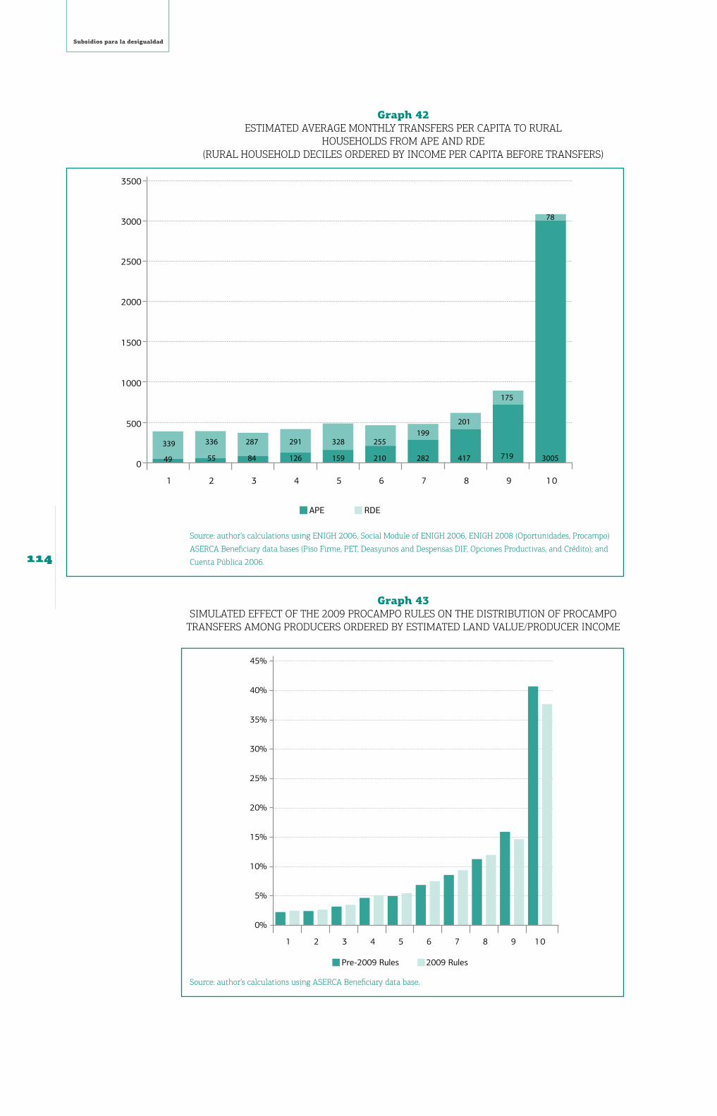
Subsidios para la desigualdad
114
Graph 42estimAteD AverAGe monthly trAnsfers Per cAPitA to rurAl
householDs from APe AnD rDe(rurAl householD Deciles orDereD by income Per cAPitA before trAnsfers)
source: author’s calculations using eniGh 2006, social module of eniGh 2006, eniGh 2008 (oportunidades, Procampo)
AsercA beneficiary data bases (Piso firme, Pet, Deasyunos and Despensas Dif, opciones Productivas, and crédito); and
cuenta Pública 2006.
Graph 43simulAteD effect of the 2009 ProcAmPo rules on the Distribution of ProcAmPo
trAnsfers AmonG ProDucers orDereD by estimAteD lAnD vAlue/ProDucer income
source: author’s calculations using AsercA beneficiary data base.
40%
35%
45%
30%
25%
20%
15%
10%
5%
Pre-2009 Rules 2009 Rules
1 2 3 4 5 6 7 8 9 10
0%
0
500
1000
1500
2000
2500
3000
3500
APE RDE
1 2 3 4 5 6 7 8 9 10
339
49
336
55
287
84
291
126
328
159
255
210
199
282
201
417
175
719
78
3005

3
Agricultural Subsidies in Mexico
115
Table 8reDistributive effects of AGriculturAl AnD rurAl exPenDitures
HH Deciles
DistributionTransfer Incidence
TransfersPre-transferincome
Post-transfer income
APE RDE + APE + RDE+ APE& RDE
APE RDE Total
Income:Unadjusted(Million MP)
108,572 76,925 467,957
1 1.6% 17.2% 2.9% 2.7% 4.9% 4.4% 14.2% 99.0% 113.2%
2 1.6% 15.8% 4.4% 3.9% 6.0% 5.3% 9.5% 57.9% 67.4%
3 2.5% 13.2% 5.5% 5.0% 6.6% 5.9% 11.2% 38.3% 49.5%
4 3.4% 12.0% 6.5% 6.0% 7.3% 6.7% 13.2% 30.4% 43.7%
5 4.0% 12.1% 7.1% 6.6% 7.8% 7.2% 13.8% 28.4% 42.2%
6 5.2% 9.4% 8.5% 8.0% 8.7% 8.2% 15.1% 18.4% 33.5%
7 6.9% 7.1% 10.0% 9.5% 9.6% 9.2% 16.8% 11.8% 28.6%
8 9.2% 6.6% 11.6% 11.2% 10.9% 10.6% 19.1% 9.2% 28.3%
9 13.4% 4.8% 13.7% 13.8% 12.5% 12.7% 23.6% 5.8% 29.3%
10 52.3% 1.8% 29.7% 33.5% 25.8% 29.7% 38.7% 1.0% 39.7%
Total 100.0% 100.0% 100.0% 100.0% 100.0% 100.0% 23.2% 16.4% 39.6%
G/CC 0.5839 -0.2652 0.3486 0.3887 0.2620 0.3118
Change in G 11.5% -24.8% -10.6%
Income: Ad-justed
(Million MP)875,291
1 2.9% 2.7% 4.0% 3.8% 7.6% 52.9% 60.5%
2 4.4% 4.1% 5.3% 5.0% 5.1% 30.9% 36.0%
3 5.5% 5.2% 6.1% 5.8% 6.0% 20.5% 26.5%
4 6.5% 6.2% 7.0% 6.6% 7.1% 16.3% 23.3%
5 7.1% 6.8% 7.5% 7.2% 7.4% 15.2% 22.6%
6 8.5% 8.2% 8.6% 8.3% 8.1% 9.8% 17.9%
7 10.0% 9.7% 9.8% 9.5% 9.0% 6.3% 15.3%
8 11.6% 11.4% 11.2% 11.0% 10.2% 4.9% 15.1%
9 13.7% 13.7% 13.0% 13.1% 12.6% 3.1% 15.7%
10 29.7% 31.9% 27.5% 29.7% 20.7% 0.5% 21.2%
Total 12.4% 8.8% 21.2%
G/CC 0.3486 0.3721 0.2990 0.3259
Change in G 6.7% -14.2% -6.5%
7. conclusIons and PolIcyrecommendatIonsThis report has analyzed the distributive incidence of the principal agricultural and rural de-velopment programs implemented in Mexico in over the last two decades, in the context of an ambitious effort to modernize the agricultural sector and address rural poverty. This “second agrarian reform” included the 1992 Ejido reform, the opening of agricultural markets through the North American Free Trade Agreement (1994-2008), the shift to more efficient and equitable agricultural support instruments, especially the delinked Procampo transfers. A similarly am-bitious and complementary reform effort in rural social policies included the introduction of effectively targeted rural programs, notably Progresa/Oportunidades, and a more general pro-rural reallocation of social spending, reversing a strong historic urban bias in the allocation of anti-poverty programs, food subsidies, basic education and health services for the uninsured.
While an evaluation of the impact of these reforms on agriculture and rural poverty in Mexico is impossible in the absence of the relevant counterfactual, especially given the broader eco-nomic context of instability and stagnation characterizing this period, the evidence on the instruments and outcomes of these policies reviewed in this report suggests that the principal challenges motivating the reforms remain in place. We will not attempt to summarize this extensive evidence here, beyond emphasizing a few basic observations:

Subsidios para la desigualdad
116
a)Today as two decades ago, a third of the rural population live in extreme poverty (pobreza alimentaria) and despite a gradual urbanization process the rural sector still accounts for a majority of the extreme poor.
b)While there is some evidence of the incipient development of rural labor and land markets, these are still hampered by structural restrictions and the lack of adequate access to other productive inputs, including credit, human capital, technology, transport and other infra-structure.
c)Despite some evidence of growth in productivity and crop diversification in line with Mex-ico’s geographic and factor comparative advantages (labor-intensive fruits and vegetables), the grain-based dual structure of agriculture has survived practically unchanged.
d)Perhaps the most dramatic transformation of the rural economy over this period is the de-cline of agriculture as a significant source of income and labor opportunities for most rural households, with public transfers, remittances, and non-farming rural activities filling the void.
Looking into the policy implications of the above analysis, it is important to note that despite its ambitious agenda the “second agrarian reform” may not have been ambitious enough in its implementation, failing to support agricultural development were it was most needed, by pro-viding critical inputs to middle-sized farmers with significant but constrained productive (and employment-generation) potential. We may identify some basic components of a “third agrar-ian reform”, directed at the three principal producer strata:
a)Considering middle-sized producers, in addition to the noted “efficiency vs. equity” concep-tual framework, an important practical restriction explaining the lack of significant produc-tive support programs reaching small to medium producers is the large heterogeneity of such producers, making the identification, implementation and monitoring of specific support “packages” difficult. This will require the development of innovative and flexible support ins-truments as well as the development of a detailed producer data base (an effort of the latter kind is currently under way at Sagarpa in collaboration with the IADB and World Bank).
b)In the case of the precarious social insurance function of subsistence farming, this should give way through the construction of effective and universal non-contributive social insur-ance schemes in the rural sector, liberating land resources to their most productive use.
c) In the case of the larger commercial producers, a case is often made in favor of maintaining or increasing support as a response to international support for competing producers and the idea of food security (“soberanía alimentaria”). But this must be carefully and explicitly weighted against competing considerations, including i) the high opportunity cost of fiscal resources in a country with low fiscal capacity, high inequality and historically low public investment, and ii) the availability of better (less distorting and inequitable) instruments to ensure domestic stability in food prices and supply while exploiting the very considerable benefits to domestic consumers from international productivity gains and subsidies. On the other hand, a case may be made for shifting support resources targeted at this producer group from private transfers to public goods, though as has been documented here such investments are already heavily concentrated on these producers.
bIblIograPHy:ASF (2006). Informe del Resultado de la Revisión y Fiscalización Superior de la Cuenta Pública
2006. Mexico: Auditoría Superior de la Federación.Avila, Antonio Flavio and Robert E. Evenson (2004). “Total Factor Productivity Growth in Agri-
culture: The Role of Technological Capital,” in Robert E. Evenson, Prahbu Pingali, and T. Paul Schultz (eds.) Handbook of Agricultural Economics. Amsterdam: Elsevier.
CEDRSSA (2009). “Apuntes sobre ejercicio del presupuesto 2007 para el sector rural,” Héctor Robles, principal investigator, Mexico: Centro de Estudios para el Desarrollo Rural Sustent-able y la Soberanía Alimentaria/DESANR/INV/009/09
CONEVAL (2008). Informe de Evaluación de la Política de Desarrollo Social en México 2008. Mexico: Consejo Nacional de Evaluación de la Política de Desarrollo Social.
Cortés, Fernando. Felipe López Calva and Rodolfo de la Torre (2005). “Evaluación de la pobreza en México”, Seminario Universitario de la Cuestión Social, Instituto de Investigaciones So-ciales, UNAM. August 24.
Cuecuecha, Alfredo and John Scott (2010). “The Effect of Agricultural Subsidies on Migration and Agricultural Employment,” Mexican Rural Development Research Report, No. 3, Wood-row Wilson International Center for Scholars, Mexico Institute, www.wilsoncenter.org/De-sarrolloRuralMexicano.
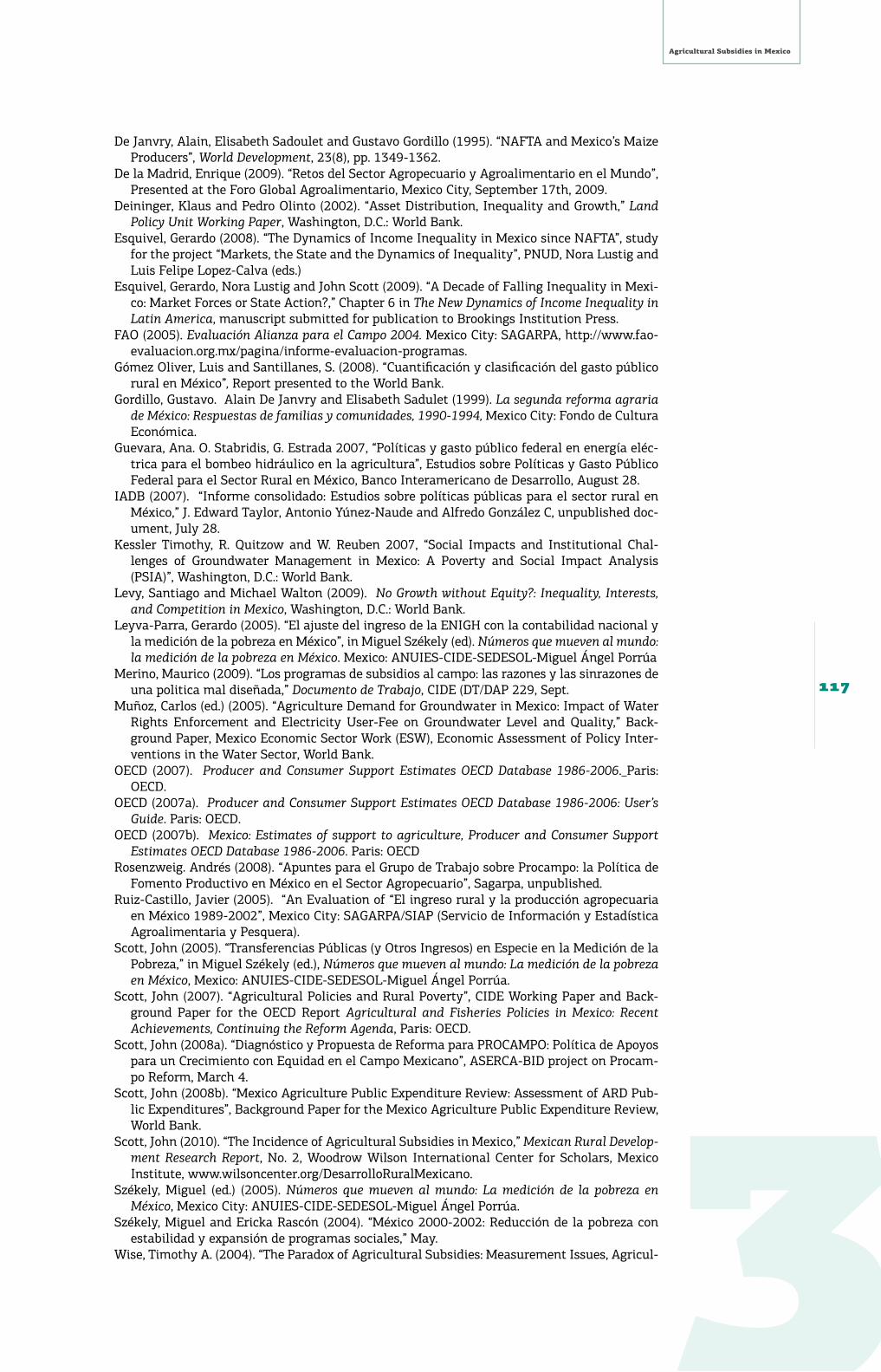
3
Agricultural Subsidies in Mexico
117
De Janvry, Alain, Elisabeth Sadoulet and Gustavo Gordillo (1995). “NAFTA and Mexico’s Maize Producers”, World Development, 23(8), pp. 1349-1362.
De la Madrid, Enrique (2009). “Retos del Sector Agropecuario y Agroalimentario en el Mundo”, Presented at the Foro Global Agroalimentario, Mexico City, September 17th, 2009.
Deininger, Klaus and Pedro Olinto (2002). “Asset Distribution, Inequality and Growth,” Land Policy unit Working Paper, Washington, D.C.: World Bank.
Esquivel, Gerardo (2008). “The Dynamics of Income Inequality in Mexico since NAFTA”, study for the project “Markets, the State and the Dynamics of Inequality”, PNUD, Nora Lustig and Luis Felipe Lopez-Calva (eds.)
Esquivel, Gerardo, Nora Lustig and John Scott (2009). “A Decade of Falling Inequality in Mexi-co: Market Forces or State Action?,” Chapter 6 in The New Dynamics of Income Inequality in Latin America, manuscript submitted for publication to Brookings Institution Press.
FAO (2005). Evaluación Alianza para el Campo 2004. Mexico City: SAGARPA, http://www.fao-evaluacion.org.mx/pagina/informe-evaluacion-programas.
Gómez Oliver, Luis and Santillanes, S. (2008). “Cuantificación y clasificación del gasto público rural en México”, Report presented to the World Bank.
Gordillo, Gustavo. Alain De Janvry and Elisabeth Sadulet (1999). La segunda reforma agraria de México: Respuestas de familias y comunidades, 1990-1994, Mexico City: Fondo de Cultura Económica.
Guevara, Ana. O. Stabridis, G. Estrada 2007, “Políticas y gasto público federal en energía eléc-trica para el bombeo hidráulico en la agricultura”, Estudios sobre Políticas y Gasto Público Federal para el Sector Rural en México, Banco Interamericano de Desarrollo, August 28.
IADB (2007). “Informe consolidado: Estudios sobre políticas públicas para el sector rural en México,” J. Edward Taylor, Antonio Yúnez-Naude and Alfredo González C, unpublished doc-ument, July 28.
Kessler Timothy, R. Quitzow and W. Reuben 2007, “Social Impacts and Institutional Chal-lenges of Groundwater Management in Mexico: A Poverty and Social Impact Analysis (PSIA)”, Washington, D.C.: World Bank.
Levy, Santiago and Michael Walton (2009). No Growth without Equity?: Inequality, Interests, and Competition in Mexico, Washington, D.C.: World Bank.
Leyva-Parra, Gerardo (2005). “El ajuste del ingreso de la ENIGH con la contabilidad nacional y la medición de la pobreza en México”, in Miguel Székely (ed). Números que mueven al mundo: la medición de la pobreza en México. Mexico: ANUIES-CIDE-SEDESOL-Miguel Ángel Porrúa
Merino, Maurico (2009). “Los programas de subsidios al campo: las razones y las sinrazones de una politica mal diseñada,” Documento de Trabajo, CIDE (DT/DAP 229, Sept.
Muñoz, Carlos (ed.) (2005). “Agriculture Demand for Groundwater in Mexico: Impact of Water Rights Enforcement and Electricity User-Fee on Groundwater Level and Quality,” Back-ground Paper, Mexico Economic Sector Work (ESW), Economic Assessment of Policy Inter-ventions in the Water Sector, World Bank.
OECD (2007). Producer and Consumer Support Estimates OECD Database 1986-2006. Paris: OECD.
OECD (2007a). Producer and Consumer Support Estimates OECD Database 1986-2006: user’s Guide. Paris: OECD.
OECD (2007b). Mexico: Estimates of support to agriculture, Producer and Consumer Support Estimates OECD Database 1986-2006. Paris: OECD
Rosenzweig. Andrés (2008). “Apuntes para el Grupo de Trabajo sobre Procampo: la Política de Fomento Productivo en México en el Sector Agropecuario”, Sagarpa, unpublished.
Ruiz-Castillo, Javier (2005). “An Evaluation of “El ingreso rural y la producción agropecuaria en México 1989-2002”, Mexico City: SAGARPA/SIAP (Servicio de Información y Estadística Agroalimentaria y Pesquera).
Scott, John (2005). “Transferencias Públicas (y Otros Ingresos) en Especie en la Medición de la Pobreza,” in Miguel Székely (ed.), Números que mueven al mundo: La medición de la pobreza en México, Mexico: ANUIES-CIDE-SEDESOL-Miguel Ángel Porrúa.
Scott, John (2007). “Agricultural Policies and Rural Poverty”, CIDE Working Paper and Back-ground Paper for the OECD Report Agricultural and Fisheries Policies in Mexico: Recent Achievements, Continuing the Reform Agenda, Paris: OECD.
Scott, John (2008a). “Diagnóstico y Propuesta de Reforma para PROCAMPO: Política de Apoyos para un Crecimiento con Equidad en el Campo Mexicano”, ASERCA-BID project on Procam-po Reform, March 4.
Scott, John (2008b). “Mexico Agriculture Public Expenditure Review: Assessment of ARD Pub-lic Expenditures”, Background Paper for the Mexico Agriculture Public Expenditure Review, World Bank.
Scott, John (2010). “The Incidence of Agricultural Subsidies in Mexico,” Mexican Rural Develop-ment Research Report, No. 2, Woodrow Wilson International Center for Scholars, Mexico Institute, www.wilsoncenter.org/DesarrolloRuralMexicano.
Székely, Miguel (ed.) (2005). Números que mueven al mundo: La medición de la pobreza en México, Mexico City: ANUIES-CIDE-SEDESOL-Miguel Ángel Porrúa.
Székely, Miguel and Ericka Rascón (2004). “México 2000-2002: Reducción de la pobreza con estabilidad y expansión de programas sociales,” May.
Wise, Timothy A. (2004). “The Paradox of Agricultural Subsidies: Measurement Issues, Agricul-

Subsidios para la desigualdad
118
tural Dumping, and Policy Reform,” Global Development and Environment Institute Working Paper 04-02, Medford, Mass: Tufts University, Global Development and Environment Insti-tute, http://www.ase.tufts.edu/gdae/policy_research/USAgPolicy.html.
World Bank (2004a). Mexico: Public Expenditure Review. Washington D.C.: World Bank.World Bank (2004b). Poverty in Mexico: An Assessment of Conditions, Trends and Government
Strategy, Washington D.C.: World Bank.World Bank (2005). Desigualdad en America Latina y el Caribe: Rompiendo con la Historia?.
Washington, D.C.: World Bank.World Bank (2006a). Poverty Reduction and Growth: Virtuous and Vicious Circles.Washington D.C.: World Bank.World Bank (2006b). Decentralization, Poverty, and Development in Mexico. Washington D.C.:
World Bank.