
Agricultural Price Transmission Across Space and...
53
XLVII Convegno SIDEA Campobasso 22-25 Settembre 2010 DRAFT 1 Agricultural Price Transmission Across Space and Commodities The Case of the 2007-2008 Price Bubble Draft Version – 15th September 2010 Roberto Esposti Department of Economics – Università Politecnica delle Marche Piazzale Martelli 8 – 60121 Ancona (Italy) e-mail: r.esposti at univpm.it; phone: +39 071 2207119 Giulia Listorti : Federal Department of Economics Affairs - Federal Office for Agriculture (FOAG) Mattenhofstrasse 5 – CH-3003 Berne (Switzerland) e-mail: giulia.listorti at blw.admin.ch Abstract This paper analyses the horizontal transmission of cereal price shocks both across different market places and across different commodities. The analysis is carried out using Italian and international weekly spot (cash) price data and concentrating the attention on years 2006-2010, a period of generalized exceptional exuberance and consequent rapid drop of agricultural prices. The work aims at investigating, on the on hand, how price transmission may be affected during price bubbles and, at the same time, how the bubble is transmitted across markets. The properties of price time series are firstly explored in depth to assess which data generation process may have eventually produced the observed patterns. Secondly, the interdependence across prices is specified and estimated adopting appropriate cointegration techniques. Key-words: Price Transmission, Price Bubbles, Time Series Properties, Cointegration JEL Classification: Q110, C320 1. Introduction: objectives and data description The main motivation of this study is to understand the properties of agricultural price series over the 2007-2008 price rally (Ec, 2008; Irwin and Good, 2009) 1 to better analyse how the prices transmitted horizontally, i.e., across market places and commodities, during the bubble and how the bubble itself has been generated and transmitted. This analysis of the horizontal price transmission during price exuberance concerns agricultural weekly spot prices and is limited to the abovementioned four years. We opt for this restriction of the time coverage for three major reasons. First of all, this period fully contains the bubble as the last observed weekly price levels (last week of April 2010) are almost equal to the first observed week (last week of April 2006). Over this period, therefore, the bubble firstly inflated and then completely deflated (Figure 1). Secondly, we can assume an almost-constant policy regime in the EU over this period. In 2006, the 2003 CAP Reform was entirely in force, included its : The views expressed in this article are the sole responsibility of the authors and do not reflect, in any way, the position of the FOAG. Authorship may be attributed as follows: sections 3.2, 3.3, 3.4, 4 and 5 to Listorti; sections 1, 2 and 3.1 to Esposti. 1 Henceforth, the “agricultural price bubble”. Heuristically, and generically, the bubble clearly appear in Figure 1. From a more rigorous point of view, however, we will formally define and test the presence of a bubble in price series in section 2.5.
Transcript of Agricultural Price Transmission Across Space and...

XLVII Convegno SIDEA Campobasso 22-25 Settembre 2010 DRAFT
1
Agricultural Price Transmission Across Space and Commodities
The Case of the 2007-2008 Price Bubble Draft Version – 15th September 2010
Roberto Esposti
Department of Economics – Università Politecnica delle Marche Piazzale Martelli 8 – 60121 Ancona (Italy)
e-mail: r.esposti at univpm.it; phone: +39 071 2207119
Giulia Listorti♣ Federal Department of Economics Affairs - Federal Office for Agriculture (FOAG)
Mattenhofstrasse 5 – CH-3003 Berne (Switzerland) e-mail: giulia.listorti at blw.admin.ch
Abstract
This paper analyses the horizontal transmission of cereal price shocks both across different market places and across different commodities. The analysis is carried out using Italian and international weekly spot (cash) price data and concentrating the attention on years 2006-2010, a period of generalized exceptional exuberance and consequent rapid drop of agricultural prices. The work aims at investigating, on the on hand, how price transmission may be affected during price bubbles and, at the same time, how the bubble is transmitted across markets. The properties of price time series are firstly explored in depth to assess which data generation process may have eventually produced the observed patterns. Secondly, the interdependence across prices is specified and estimated adopting appropriate cointegration techniques.
Key-words: Price Transmission, Price Bubbles, Time Series Properties, Cointegration JEL Classification: Q110, C320
1. Introduction: objectives and data description
The main motivation of this study is to understand the properties of agricultural price series over the
2007-2008 price rally (Ec, 2008; Irwin and Good, 2009)1 to better analyse how the prices transmitted
horizontally, i.e., across market places and commodities, during the bubble and how the bubble itself
has been generated and transmitted. This analysis of the horizontal price transmission during price
exuberance concerns agricultural weekly spot prices and is limited to the abovementioned four years.
We opt for this restriction of the time coverage for three major reasons. First of all, this period fully
contains the bubble as the last observed weekly price levels (last week of April 2010) are almost equal
to the first observed week (last week of April 2006). Over this period, therefore, the bubble firstly
inflated and then completely deflated (Figure 1). Secondly, we can assume an almost-constant policy
regime in the EU over this period. In 2006, the 2003 CAP Reform was entirely in force, included its
♣ The views expressed in this article are the sole responsibility of the authors and do not reflect, in any way, the position of the FOAG. Authorship may be attributed as follows: sections 3.2, 3.3, 3.4, 4 and 5 to Listorti; sections 1, 2 and 3.1 to Esposti. 1 Henceforth, the “agricultural price bubble”. Heuristically, and generically, the bubble clearly appear in Figure 1. From a more rigorous point of view, however, we will formally define and test the presence of a bubble in price series in section 2.5.

XLVII Convegno SIDEA Campobasso 22-25 Settembre 2010 DRAFT
2
limited implications in terms of price policy and market intervention; the regime then remained
constant over the whole 2006-2010 period. The only relevant policy regime change over the period
under consideration has been the temporary suspension of EU import duties on cereals from January
2008 to October 2008. This change, in fact, was justified by price movements themselves (the bubble).
Therefore, in investigating price transmission during the bubble it is also possible to assess the role
played by this single policy measure whose application is confined into a limited number of months.
Finally, concentrating on this period facilitates international price comparison as the cumulative
inflation rate has been quite limited and relatively similar in Italy and in North-America (the two areas
under study here). Therefore, comparison of agricultural prices across different countries does not
require the deflation of nominal prices into a common real base.
The dataset here adopted is made of cereal weekly spot price series observed in different Italian
locations (from North to South) (source: ISMEA) and in international (North-American) markets
(source: International Grain Council, IGC). Commodities under consideration are soft wheat, durum
wheat, barley and corn (with soft and durum wheat possibly distinguished in different quality grades).
Therefore the dataset dimensions are: T = 210 weeks (from last week of April 2006 to last week of
April 2010); K commodities; N market places, that is North-Italy (Milan), Centre-North Italy
(Bologna), Centre-South Italy (Rome), South-Italy (Catania, Foggia, Naples), US and Canada (or
Rotterdam; see below). In practice, the dataset has a Tx(NxK) size. Table A1 (Appendix) details the
NxK = 28 price series under investigation and their respective acronyms.
To facilitate comparisons and analysis of transmission, international and national prices have to be
expressed in a common currency. Therefore, US and Canadian prices have been converted from US
dollars to Euros by taking the weekly official $/€ exchange rate provided by Eurostat-ECB.2 These
North-American prices actually are FOB prices. For agricultural commodities, the ratio of freight rates
on FOB prices is quite high and it also considerably oscillated during the commodity price bubble
(especially due to volatility in energy, namely oil, prices). According to this, freight rates (source:
IGC) were added to US and Canadian prices in order to obtain the respective CIF prices. The freight
rates used in this study are those from US Gulf (or Canada, where applicable) to ARAH (i.e,
Amsterdam/Rotterdam/Antwerp/Hamburg destinations). In practice, in our analysis the North-
American prices actually serve as international price taken at Rotterdam, thus as EU-reference prices.
Henceforth, we will refer to international prices as Rotterdam prices (see Table A.1).
Figure 1 reports the 28 price series over the period under investigation here. Simple inspection clearly
reveals the price bubble and that the price exuberance concerned almost all markets but with a
remarkable different intensity. A proper empirical analysis of price transmission over this period,
therefore, requires two steps. First of all, the time-series properties of these agricultural prices have to
be carefully investigated to understand which process can have eventually generated the explosive
2 It implies that adjustments to the exchange rate are considered instantaneous.
XLVII Convegno SIDEA Campobasso 22-25 Settembre 2010 DRAFT
3
pattern and the consequent drop, and for which prices we can look for a common behaviour and,
therefore, for interdependence (section 2). Then, such interdependence across markets (commodities
and places) is specified (section 3) and estimated (section 4) within a proper cointegration framework.
Section 5 concludes.
2. Some basic evidence on agricultural price behaviour
High frequency (daily or weekly) agricultural price series combine the properties of lower-frequency
(monthly or annual) agricultural price series with the typical properties of financial series (Wei and
Leuthold, 1998). In short, agricultural price series often maintain characteristics that are naturally
attributed to agricultural products and markets (Wright, 2001), namely, seasonality and long memory
(i.e, high persistence of shocks over time, but no evident short-run cycles) and, sometimes, even
chaotic behaviour in the longer run (Wei and Leuthold, 1998). At the same time, other features,
usually attributed to the specific nature of financial markets, may be detected as well: changing
volatility (i.e., changing price variance), non-stationarity (i.e., prices following random walk
behaviour) and temporary (and even periodic) exuberance or explosive behaviour (the bubbles).
The combination of these properties may generate very peculiar patterns and, in particular, nonlinear
dynamics. In practice, they can be often hardly distinguishable and separated especially whenever they
partially overlap. As these features may characterize most agricultural commodities and markets, they
also make the identification of market interdependence (i.e., how they affect each other) particularly
difficult as a given price movement can be attributed to either own price dynamics or to response to
other markets’ variations. This is even more true over period of price bubbles, that is, of strongly
nonlinear dynamics with rapid (and apparently unexpected) price increase soon followed by a period
of as much intense price drop. More specifically, during such periods of exuberance, the identification
issues becomes whether the typical abovementioned behaviour of high-frequency agricultural price
series experiences a structural change or, on the contrary, bubbles are nothing but “normal” outcomes
of the interactions among these typical characters.
Therefore, before entering the analysis of how market prices interact, thus reciprocally transmitting
price shocks, it seems rational to firstly assess the time series properties of the prices under study. This
analysis not only allows identifying those prices showing common features but it is also needed to
achieve a proper specification of price transmission/interdependence relations.
Let consider agricultural prices observed over these three different dimensions: space, commodity and
time. The generic price is, therefore, tkip ,, where i=1,…,j,…,N is the (local) market (spatial
dimension); k=1,…,h,…,K is the commodity; t=1,…,s,…,T is the period of observation (time
dimension). By more conventionally distinguishing between a cross-sectional dimension, given by the
combination of the dimensions ik, and a time dimension t, we can identify any generic price
observation as tikp , (scalar) and any generic price series (vector) as ikp . Through a sequence of

XLVII Convegno SIDEA Campobasso 22-25 Settembre 2010 DRAFT
4
testing procedures, this section aims at detecting the abovementioned properties of time series ikp .
Both price levels ( ikp ) and logarithmic transformations (iklp ) are considered and in both cases, if
needed, tests are repeated on the respective first-order differences ( ikp∆1 and iklp∆1 ) to observe
whether the abovementioned features remain or vanish after differentiation.
The analysis of price patterns, and of their nonlinear dynamics, is performed by testing, in sequence,
their distributional properties (normality), seasonality, volatility (ARCH effects), stationarity,
persistence (long memory or fractional integration) and explosiveness. All these features may be
responsible for nonlinear dynamics and, therefore, may be invoked as possible causes of the observed
exuberance. At the same time, they also imply different stochastic processes and price
interdependence.
2.1. Normality, seasonality and structure of autocorrelation
Some of the typical properties of high-frequency agricultural price series may imply nonlinear
dynamics that, in turn, induces non normal unconditional distributions usually showing strong
skewness and fat tails (Wei and Leuthold, 1998). Therefore, testing for unconditional normality of
price series is a basic and simple way to detect the presence of such nonlinearities. Table 1 reports
normality tests on price series (in both levels and logarithms) suggesting that in all cases we can reject
the hypothesis of underlying normal unconditional distribution. Test also confirm the presence of
skewness and fat tails as could be easily expected over a period of price exuberance and rapid drop
(the bubble).
A period of relatively long exuberance not only affect the distributional properties of agricultural price
series, but also influences another of their typical characters, namely, the presence of short-run (within
year) cycles or recurrence. Previous studies on similar markets and data frequency (weekly or even
monthly prices) (Verga and Zuppiroli, 2003, and Listorti, 2007, 2009, respectively) show that cereal
markets are often characterised by a significant seasonality. The presence of these seasonal (or other
short-run) cycles is not surprising considering that, especially in national markets, production is
concentrated in a specific part (just few weeks) of the year while prevalent uses are homogeneously
distributed over the year. This inevitably generates, even for highly storable commodities like cereals,
a cyclical seasonal behaviour of prices. Seasonality in series ikp would imply that an observation at a
given time t, tikp , , shows a significant partial autocorrelation not only with closer observations
( 1, −tikp , 2, −tikp , etc.) but also with observations far-away in time, stikp −, , with s usually taking values
close to 45-50 expressing the seasonal recurrence.
Table 2 reports selected results emerging from the estimation of the Partial AutoCorrelogram (PAC) of
prices under study. Series behaviour is pretty similar across all prices. In all cases, partial
autocorrelation coefficients are significant within few lags (2 or 3 in most cases) and particularly high

XLVII Convegno SIDEA Campobasso 22-25 Settembre 2010 DRAFT
5
(close to 1) for lag t-1, but no clear short-run (within year) cycles comes out, though in few cases we
can observe significant partial correlation coefficients for lags between 45 and 50 weeks. Therefore,
seasonal recurrence does neither clearly nor homogeneously emerge and, when and if present (mostly
in international prices), only weakly influences the price pattern over the period. This conclusion is
also easily detectable by taking, for any week, the average price over observed years. Figure 2 displays
these 52 average prices for the whole period and for the two sub-periods (April 2006- April 2008;
April 2008-2010), that is, for the ascending and the descending parts of the price bubble. Price
averages does not significantly change over the year. No sharp drop or rise is observed in
correspondence to seasonal recurrences.
This evidence is at odds with previous results on weekly data of national and international cereal
markets (Verga and Zuppiroli, 2003) but should not surprise for two basic reasons. First of all, the
period under consideration covers just four years, thus four possible seasonal recurrences. Even from a
strictly statistical point of view, seasonal patterns can be hardly detected with such limited number of
events. A secondly, and more important, reason is that the bubble itself, and the nonlinearities
associated to this, may hide a slight seasonality. This is illustrated in the lower part of Figure 2. In the
two sub-periods, average prices actually change over the year and, in particular, regularly increases in
the first two years and then regularly declines in the second sub-period. No clear discontinuity is
observed. This is perfectly consistent with the formation of the bubble and has almost nothing to do
with real seasonal patterns.
Therefore, considering the limited number of years under investigation and that, even when present, it
only marginally affects the observed price patterns, seasonality will be ignored henceforth.3
2.2. Stationarity
Regardless the presence of seasonal or other short-term cycles, what really matters in understanding
the behaviour of price series especially in a period of such dramatic exuberance and drop, is the
presence of unit and/or explosive roots. Stationary (i.e. I(0)) series can be hardly reconciled with the
formation of the bubble. Even stationarity around a drift (a constant term) and/or a deterministic trend
is not evidently helpful in this respect. Figure 1 shows, in particular, how the presence of a
deterministic trend can be easily excluded by a simple visual inspection of the series themselves. As
will be clarified below, testing for the presence of a temporary explosive pattern can not be simply
achieved through conventional unit-root tests. Nonetheless, albeit not sufficient, these latter tests still
3 The exception are unit-root tests (Table 3) in which we still include seasonal dummies as their exclusion, in those cases where they are significant, may affect test validity. In general terms, though not presented here (they are available upon requests), all tests and estimates reported in the present paper have been also obtained by introducing seasonal dummies. This additional evidence suggests that all results are robust with respect to seasonality: the coefficients associated to dummies are always hardly significant and, in any case, results do not change significantly.

XLVII Convegno SIDEA Campobasso 22-25 Settembre 2010 DRAFT
6
allow assessing a necessary outcome of nonlinearities within price series: series turn out to be I(1) and
not I(0) (Diba and Grossman, 1988; Evans, 1991; Phillips and Magdalinos, 2009; Philips et al., 2009;
Phillips and Yu, 2009; Gutierrez, 2010).
Table 3 thus reports unit root tests on ikp , iklp , ikp∆1 and iklp∆1 . Two different tests are run, the
ADF and the PP tests (Enders, 1995), as the latter is expected to be more robust under
heteroskedasticity which may, in fact, occur (see below the test on ARCH effects). In general terms, it
looks like that, once the proper specification has been selected (in terms of admitted lags and of
presence of drift and deterministic trend), all ikp and iklp
series show a unit root. On the contrary, all
ikp∆1 and iklp∆1
series are stationary. The conclusion would be that all price series can be
considered I(1) but not I(2).
I(1) series (random walks possibly with a drift and/or a deterministic trend), however, are apparently
at odds with the evidence of a price bubble, as they can hardly generate temporary explosive
behaviour. More generally, it remains to explain how such I(1) ikp series may have eventually
generated the observed price pattern in all markets (Figure 1). Three possible explanations can be
considered in this respect. The first is that I(1) series generate the observed pattern due to a sudden and
temporary increase in volatility, namely, of price variance. The second explanation is that ikp∆1 and
iklp∆1 are, in fact, neither I(0) nor I(1) series (therefore ikp is neither I(1) nor I(2)). They could rather
show fractional integration (or long-memory), that would make sudden exogenous price shocks
persistent over long time (i.e, many weeks). A final explanation is that, as conventional unit-root tests
can not really assess (or exclude) the presence of temporary explosive roots (the bubble), more
appropriate ad hoc tests should be adopted.
2.3. Increasing volatility
One possible reconciliation of I(1) series with nonlinearities implied by bubbles can be found in the
presence of ARCH effects (Hamilton, 1994; Enders, 1995). The observed behaviour of price series
could be attributed to I(1) series showing a dramatic increase in volatility during the bubble. ARCH
theory admits the nonormality of the unconditional distribution of the data emerging in Table 1 (Wei
and Leuthold, 1998, p. 15) and the presence of ARCH effects does not prevent the use of ADF test to
assess nonstationarity. Therefore, series could be correctly assumed I(1) still in the presence of ARCH
effects. One way to assess the hypothesis that series ikp ( iklp ) originate from a combination of
random walk and autoregressive conditional heteroskedasticity consists in testing the presence of such
ARCH effects in ADF regressions (Table 3).
For the generic price tikp , , the ADF regression, possibly with drift ikµ and deterministic trend t, is
specified as usual:

XLVII Convegno SIDEA Campobasso 22-25 Settembre 2010 DRAFT
7
(1) tikik
S
sstikistikikiktik etppp ,
21,1,, ++∆++=∆ ∑
=+−− βπρµ
where 0=ikρ under the null of unit-root process, while it is expected to be <0 for stationary process
and >0 under explosive roots. If an ARCH is admitted, however, the distribution of usual error term
tike , instead of being assumed i.i.d N(0,σ2), behaves according to an ARCH(m) process:
(2) tike , ∼ N(0, hik) where ∑=
−+=m
sstiksik eh
1
2,0 θθ with mss ,...,10,00 =∀≥> θθ
Testing for the presence of an ARCH effect thus means to perform an LM test on this heteroskedastic
structure of the error term. Table 4 reports these ARCH tests on ADF regressions for both ikp and
iklp . Results are mixed but, particularly in the logarithmic transformation, there is a clear prevalence
of series for which the ARCH effect can be rejected. In practice, only for corn and for international
prices we observe a generalised evidence of an ARCH effect. For all other series, changing volatility
in I(1) series does not provide, in any case, an explanation of the observed behaviour of prices over the
period. On the contrary, in principle, in those series for which ARCH effects are present, the
combination of I(1) series with varying volatility may remains a plausible justification. Nonetheless,
though to a different extent, the price exuberance and fall during years 2007-2008 is generalised across
almost all cereal markets under investigations here. It clearly emerge also for prices for which an
ARCH effect is excluded (durum wheat, for instance, shows the largest bubble among all cereals). We
could admit that exuberance was originally generated in markets with the ARCH effects and then
transmitted to other markets. It is not clear, however, why such transmission did not imply even the
change in volatility.
Analysing this latter aspect goes beyond the scopes of the present analysis. Benavides (2004) provides
an example of a Multiple GARCH approach to agricultural commodity markets to analyse price
interdependence even in terms of changing volatility. It must be noted, however, that such kind of
analysis, is much more frequent and suitable for higher-frequency price series whose patterns (and
underlying mechanisms) are very close to purely financial markets. This is clearly the case of future
prices of agricultural commodities (see Wei and Leuthold, 1998; future prices rather spot prices are, in
fact, investigated by Benavides, 2004) while it seems less suited for monthly or weekly agricultural
spot prices under study here.
2.4. Long memory (fractional integration)
As emphasized by Wei and Leuthold (1998), agricultural prices (and, in particular, future prices) are
often characterised by long memory that may also generate non-linear patterns quite close to chaotic
processes. In such cases, strictly speaking, price series are neither I(0) nor I(1) as they are rather I(d)
processes, with 0<d<1 (fractional integration). Conventional unit-root tests may fail in assessing

XLVII Convegno SIDEA Campobasso 22-25 Settembre 2010 DRAFT
8
whether price series are I(0) or I(1) while, in fact, they are I(d) The presence of fractional integration
thus may be not excluded in allegedly I(0) series with long persistence of shocks. Originally proposed
by Granger and Joyeux (1980), the idea of fractional integration implies that, though not behaving as
random walk (where shocks never vanish over time), price series keep the memory of a given shock
for a long period. Roughly speaking, the importance of market information (price shocks) does not
decay (or very slowly decay) over time.
This kind of stochastic process assumes specific interest here as it may be consistent with evident
nonlinearities and time-varying variances within price series. In particular, I(1) price series with or
without ARCH effects can generate the nonlinearities observed during the bubble when fractional
integration occurs in the first differences. In such case, though an unit root in first-differenced series
can not be detected, a long-memory process would still imply strong persistence of momentary shocks.
The presence of such long memory within the price series can be tested following the approach
originally proposed by Geweke and Porter-Hudak (1983) and then modified by Phillips (1999a,b).
Such test is based on a particular representation of the stochastic process generating the generic price
series ikp or its first differences ikp1∆ . This representation is called ARFIMA(p,d,q) (Autoregressive
Fractionally Integrated Moving Average) model. In the case of ikp1∆ the AFIMA(p,d,q) model is
specified as follows:
(3) ( ) tik
q
s
sstik
dp
s
ss LpLL ,
1,
1
111 εθα
−=∆−
− ∑∑
==
where L is the usual lag operator. αs are the parameters of the autoregressive part of the model, θs the
parameters of the moving average part. tik ,ε is a conventional normally distributed spherical
disturbance. If a series exhibits long memory, it is neither a I(0) nor a I(1) process; it is an I(d) process.
By testing for the value of parameter d, the test proposed by Phillips (1999a,b), and here adopted, can
distinguish among stationary, unit-root and fractionally integrated processes. The procedure produces
two test statistics, one for the null d=0 and one for d=1. If d=0 is accepted the series is stationary; if
d=1 is accepted the series has an unit root. If both are rejected (namely, if 0<d<1), then fractional
integration (long memory) is accepted.
Results of these tests are reported in Table 5. Test results confirm that, when applied to original series,
unit root is evidently observed. When applied to first differences (either in the levels or in the
logarithmic transformations), the presence of unit root is always rejected but in few cases (and in all
international prices) the presence of fractional integration cannot be excluded. This would suggest
that, although no evidence emerge in favour of ikp (or iklp ) as I(2) series, at least some prices are
“something more” than I(1) series as their first differences show long memory, therefore long
persistence of shocks. Long-memory (fractionally integrated) processes are expected to show
relatively low but constant and long-lasting autocorrelations (Wei and Leuthold, 1998, p. 14). If

XLVII Convegno SIDEA Campobasso 22-25 Settembre 2010 DRAFT
9
observed in the first difference ( ikp∆1 ), this property may generate the temporarily non-linear pattern
observed in the recent years in cereal markets. Once more, however, as the support to such behaviour
is not generalized (that is, is only observed in few prices), it remains hard to explain why, on the
contrary, the exuberance is, in fact, generalized across the markets. Even assuming that shocks are
transmitted across markets, the long memory character should itself be transmitted to all markets.4
2.5. Testing explosiveness: recursive unit root tests
The analysis carried out so far attempted to identify those possible common stochastic processes that
may have generated the price patterns observed in the recent years. Although, given test results, we
may be confident on the fact that ikp (or iklp ) behave as I(1) processes. It is also clear that there must
be “something more” beyond unit roots in price series to explain the exuberance and rapid drop (thus
temporary nonlinear dynamics) recorded during the so-called price bubble. Possible explanations
(ARCH effects in price levels of long memory in price first differences) may provide a possible
explanation only in some cases while, in fact, the temporary nonlinear dynamics we are trying to
explain is generalized across all observed cereal markets.
A final and, in fact, more intuitive explanation could simply be that the observed dynamics is
generated by unit root processes in which an explosive root temporarily overlaps. A more formal and
rigorous definition of a temporary (or periodically collapsing) bubble in price or financial series
consists in the presence of temporary explosive roots. Such temporary explosive patterns present a
problem to standard time series analysis. In time-series econometrics, non-stationary variables are
usually assumed to be either first-order integrated, I(1), or second-order integrated, I(2), or perhaps
fractionally integrated processes (Engsted, 2006). Nonlinear patterns, in fact, could more naturally
emerge from I(2) processes. Nonetheless, a price series showing a period of explosive behaviour (a
temporary bubble) is not necessarily an I(2) series. On the contrary, a I(2) process would imply a
permanent exuberance of prices while, in fact, the observed bubble inflates and deflates within a
relatively limited period of time.
Bubbles induce a temporary explosive root in price series in addition to a unit root. The problem, once
more, is that price series containing a temporary exuberance do behave neither as I(1) processes nor as
I(2) processes and, therefore, if this additional root is not appropriately considered, conventional
testing may fail in detecting the real underlying stochastic process (Evans, 1991).
Recent works by Phillips and Magdalinos (2009), Philips et al. (2009) and Phillips and Yu, 2009 (see
also Gutierrez, 2010) have provided an appropriate framework for assessing the presence of an
explosive root (a bubble) within processes that would be otherwise ruled as I(1). They propose a test
4 As for the ARCH effect, even the presence of long memory in agricultural price series is more often mentioned in the case of future prices rather than spot prices (Wei and Leuthold, 1998).
XLVII Convegno SIDEA Campobasso 22-25 Settembre 2010 DRAFT
10
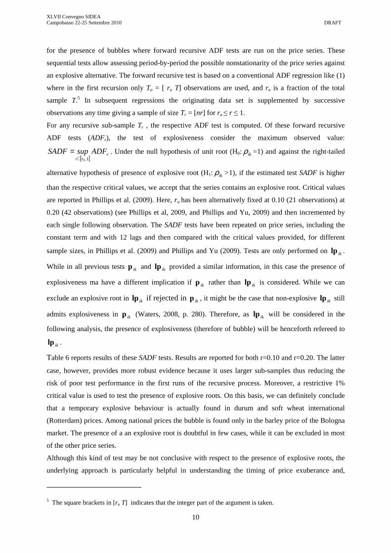
for the presence of bubbles where forward recursive ADF tests are run on the price series. These
sequential tests allow assessing period-by-period the possible nonstationarity of the price series against
an explosive alternative. The forward recursive test is based on a conventional ADF regression like (1)
where in the first recursion only To = [ ro T] observations are used, and ro is a fraction of the total
sample T.5 In subsequent regressions the originating data set is supplemented by successive
observations any time giving a sample of size Tr = [nr] for ro ≤ r ≤ 1.
For any recursive sub-sample Tr , the respective ADF test is computed. Of these forward recursive
ADF tests (ADFr), the test of explosiveness consider the maximum observed value:
[ ]r
rr
ADFsupSADF1,0∈
= . Under the null hypothesis of unit root (H0: ikρ =1) and against the right-tailed
alternative hypothesis of presence of explosive root (H1: ikρ >1), if the estimated test SADF is higher
than the respective critical values, we accept that the series contains an explosive root. Critical values
are reported in Phillips et al. (2009). Here, ro has been alternatively fixed at 0.10 (21 observations) at
0.20 (42 observations) (see Phillips et al, 2009, and Phillips and Yu, 2009) and then incremented by
each single following observation. The SADF tests have been repeated on price series, including the
constant term and with 12 lags and then compared with the critical values provided, for different
sample sizes, in Phillips et al. (2009) and Phillips and Yu (2009). Tests are only performed on iklp .
While in all previous tests ikp and iklp
provided a similar information, in this case the presence of
explosiveness ma have a different implication if ikp rather than iklp
is considered. While we can
exclude an explosive root in iklp if rejected in ikp , it might be the case that non-explosive iklp still
admits explosiveness in ikp (Waters, 2008, p. 280). Therefore, as iklp will be considered in the
following analysis, the presence of explosiveness (therefore of bubble) will be henceforth refereed to
iklp .
Table 6 reports results of these SADF tests. Results are reported for both r=0.10 and r=0.20. The latter
case, however, provides more robust evidence because it uses larger sub-samples thus reducing the
risk of poor test performance in the first runs of the recursive process. Moreover, a restrictive 1%
critical value is used to test the presence of explosive roots. On this basis, we can definitely conclude
that a temporary explosive behaviour is actually found in durum and soft wheat international
(Rotterdam) prices. Among national prices the bubble is found only in the barley price of the Bologna
market. The presence of a an explosive root is doubtful in few cases, while it can be excluded in most
of the other price series.
Although this kind of test may be not conclusive with respect to the presence of explosive roots, the
underlying approach is particularly helpful in understanding the timing of price exuberance and,
5 The square brackets in [ro T] indicates that the integer part of the argument is taken.

XLVII Convegno SIDEA Campobasso 22-25 Settembre 2010 DRAFT
11
therefore, to eventually date the beginning and the end of the price bubble. To locate the origin and the
conclusion of the exuberance, one can display the series of the abovementioned forward recursive
ADFr test and check if, when and how long ADFr exceeds the right-tailed critical values of the
asymptotic distribution of the standard Dickey–Fuller t-statistic (Phillips et al. 2009). Still adopting a
restrictive 1% critical value, Figure 3 reports this evidence and clearly shows that the price bubble in
national markets is limited to very few cases and lasts for a very short period not overlapping with the
period of suspension of the EU import duties on cereals. In international markets, the price bubble
involves more commodities and its duration is much longer clearly overlapping with the period of
suspension of the EU import duties on cereals.
According to these results, and following restrictive criteria as explosiveness may be easily confused
with different processes generating similar patterns (as in the case of possible fraction integration of
iklp∆1 for international prices), we will henceforth consider that only prices l_or_bo, l_cwad_can,
l_cwrs_can and l_dns_us (see Table A1; l_ indicates that they are logarithms) clearly contain an
explosive root. Of these, however, l_cwrs_can and l_dns_us will be not used in the following analysis
(see Table A.2). The period of the bubble is assumed to start in the first week of July 2007 and finish
in the last week of March 2008. In all other price series, the observed nonlinear dynamics should be
attributed to the other kinds of stochastic processes that have been tested in this section (or to a
combination of them).
[Table 6 here]
[Figure 3 here]
3. Modelling price interdependence as price transmission mechanisms
In the previous section, a large number of different cereal price series have been investigated at the
research of a stochastic process that may have generated their relatively homogenous behaviour over
the last years. Some evidence emerged in favour of the presence of “something more” than a simple
I(1) process, but this evidence is not concordant across all prices. The paradox, therefore, is that
although cereal prices clearly moved together, despite differences, over time (see Figure 1), the price-
by-price analysis performed so far did not find any clear common feature for ikp (or iklp ) except the
fact that they all seems to be I(1) series.
One possible way to deal with this apparent paradox, however, is to directly look for linkage
(interdependence) across prices rather than examining their individual properties then looking for
some common properties. After all, beyond visual inspection, there is very clear evidence of a strong
interdependence across markets of both different commodities (same place) and difference places
(same commodity). Table 7 reports the (NKxNK) correlation matrix across prices (ikp ). Price
correlation is evidently high not only within the same commodity but also across different

XLVII Convegno SIDEA Campobasso 22-25 Settembre 2010 DRAFT
12
commodities in the same market place. This is not in any conclusive as this strong correlation among
I(1) series can be, in fact, spurious. Nonetheless, a generalized correlation across prices is confirmed
by the fact that the error terms of the ADF regressions (1) themselves show a very strong cross-
sectional correlation. Performing the Pesaran (2004) test for cross-sectional correlation (CD test; H0:
no cross-sectional correlation) on error terms of the ADF equations of Table 3, we obtain the
following results: 45,98 and 47,56 (with the constant term), 46,07 and 47,99 (without the constant
term) for ikp and iklp , respectively. All these test values are largely statistical significant at the 1%
confidence level.
More generally, there is a diffuse evidence of a strong linkage across price series. Asking whether this
linkage is just a spurious evidence or can be interpreted as a real interdependence across cereal
markets in both the space and commodity dimensions, inevitably leads to specify which form this
interdependence is expected to take and, then, to test and estimate it.
3.1. A general model of price transmission
Let us consider the generic agricultural price tkip ,, . The behaviour of tkip ,, over its three dimensions
might be evidently represented within appropriate structural models as the combination of market
fundamentals such as supply, demand and stock formation. But such models are inherently very
complex and hardly tractable in the empirical analysis, whereas the analysis of price evolution and
linkage is more frequently afforded within reduced-form model. For example, Fackler and Goodwin
(2001) provide a common template embracing all dynamic regression models, based on linear excess
demand functions, from which an estimable reduced-form model (in their case, a VAR in prices) can
be eventually derived within this framework. Reduced-form models are actually and by far more
feasible and of immediate use to generate price predictions on the basis of the available observations
and when the three dimensions are explicitly considered, i.e., to estimate
( )stkisthistkjtki ppppE −−− ,,,,,,,, ,, .
A generic reduced-form model of price formation and transmission over the three dimensions can be
represented as follows:
(4a) tki
TSs
ssthjkh
skh
TSs
sstkjij
sij
TSs
sstkiskitki pppp ,,
0,,
0,,
1,,,,, εϖωρα ++++= ∑∑∑∑∑
<=
=−≠
<=
=−≠
<=
=−
where tki ,,ε ∼ ( )2,,,0 tkiN σ . Equation (4a) can be rewritten, as mentioned, in a more conventional form
by distinguishing a cross-sectional dimension (given by the combination of the dimensions ik) and a
time dimension, t. Therefore, we are interested in a reduced-form model predicting the expected value
of the generic price ( )stikstjhtik pppE −− ,,, , and (4a) becomes:

XLVII Convegno SIDEA Campobasso 22-25 Settembre 2010 DRAFT
13
(4b) tik
TSs
sstjhikjh
sjhik
TSs
sstiksiktik ppp ,
0,,
1,, εωρα +++= ∑∑∑
<=
=−≠
<=
=−
where tik ,ε ∼ ( )2,,0 tikN σ . Equation (4b) can be written in a more compact matrix form:
(4c) t
TSs
sss εWPαP ++= ∑
<=
=0
where P , sP and tε are (Tx(NxK)) matrices, s expresses the time lag, α is a (Tx(NxK)) matrix of
time invariant parameters, that is, sjiααα ikstiktik ,,,,, ∀== − (any column of α contains T elements
with constant value ikα ) and tε ∼ ( )tN Ω0, . sW is a ((NxK)x(NxK)) matrix of unknown parameters
incorporating the correlation across prices within both the time and space-commodity dimensions. The
diagonal elements, sikik ,ω , actually represent the auto-correlation over time, with the exclusion of the
matrix 0W , where diagonal elements are evidently ikikik ∀= ,00,ω . The off-diagonal elements, s jhik ,ω ,
represent the cross-sectional dependence of prices; in other words, they express the degree of common
movement shown by different prices and, therefore, the degree and the direction at which price shocks
are transmitted.6
In particular:
- if h=k but i≠j, we are considering the spatial price transmission for the same commodity across
different market places. In this case, under perfect spatial arbitrage, the Law of One Price (LOP)
holds and we may expect jkik ,ω =1 ;
- if i=j but h≠k, we are considering the price transmission between different commodities in the
same market. In this case, elements ihik ,ω indicate the degree of substitutability between the
different goods (Dawson et al., 2006). ihik ,ω will be close to 1 under perfect substitutability
between h and k, while it will be close to 0 under low substitutability.
If model (4a-c) is specified in tlP (the matrix of price logarithms), elements of sW indicate the price
transmission elasticities that is, how much of a percentage variation in stikp −, is transmitted to tjhp , .
Within logarithmic form, the implicit assumption is that all factors possibly contributing to price
differentials but not explicitly taken into account in the model (for example, transportation and
transaction costs) are a constant proportion of prices. Elements of α indicate these constant
multiplicative terms (that can be naturally intended as percentages) applied to price stikp −, to obtain
tjhp , .
6 See Fackler and Goodwin (2001), for a comprehensive description. Indeed, the study of price transmission mechanisms implies referring to a number of economic concepts for which no common definitions exist in literature.

XLVII Convegno SIDEA Campobasso 22-25 Settembre 2010 DRAFT
14
If matrix of unknown parameters, sW , contains all information about price linkages over the three
dimensions, we can expect that (4a-c) gets rid of autocorrelation and heteroskedasticity across both the
time and cross-sectional dimensions, that is, it restores spherical error terms: tε ∼ ( )I0 σ,N and
( ) 0, =−sttE εε . The proper specification of (4a-c), therefore, should aim at restoring such conditions.
3.2. Model specification
The first specification issue concerning model (4a-c) has to do with its size. With 28 price series, the
size of sW becomes particularly large especially whenever several lags (due to weekly data) had to be
admitted. To reduce the size of the problem (and the number of parameters to be estimated),
assumption can be made about the relevant interactions to be considered. Therefore, also to facilitate
the economic interpretation of the results, the analysis of the price interdependence have to be
“confined” and “segmented”. In particular, we may firstly assume that price transmission only occurs
within the same commodity (that is, ikp and jkp are interdependent) and within the same market
place (that is, ikp and ihp are interdependent). The consequent assumption is that ikp and jhp have
no direct linkage. This implies fixing at 0 some of the elements of the 0W matrix. Secondly, the
relation across prices can be separately studied by group of commodities segmenting the analysis
within the fixed-commodity/cross-space(market) dimension ( ikp , jkp ) from the analysis within the
fixed-space(market)/cross-commodity dimension (ikp , ihp ). Table A.2 in the Appendix details the
groups of prices whose interdependence has been considered.7
The conclusion achieved in the testing section, that all series iklp can be considered I(1) processes
with some of them also showing a temporary bubble, must be appropriately taken into account when
developing, specifying and estimating model (4a-c). Actually, agricultural commodity price series are
often found to be I(1); for this reason, since the seminal work of Ardeni (1989), cointegration
techniques have been extensively used for the study of price transmission mechanisms. Cointegration
models presuppose that variables exhibiting nonstationary behaviour will nonetheless be linked by a
long run relation, whose residuals are stationary. When fixed-commodity and cross-market price
relations are considered, under perfect spatial arbitrage, this relation is the LOP, which is expected to
hold in the long-run (LR) despite in short-run (SR) prices are allowed to deviate from it.
In the cointegration context, it is possible to take care of both issues raised by the presence of the
bubble. On the one hand, separating the LR and SR price interdependence allows identifying what
links prices outside and beyond the bubble from the temporary linkages caused by the bubble. On the
7 Some of the 28 price series here available (see Table A.1) are not used in the empirical analysis as they are highly redundant (in particular prices of different qualities of soft and durum wheat are almost coincident)

XLVII Convegno SIDEA Campobasso 22-25 Settembre 2010 DRAFT
15
other hand, we may ask to what extent the bubble itself affected the structural (LR) linkages across
prices. This can be achieved by firstly testing for the presence of cointegration and, then, estimating
appropriate Vector Error Correction Models (VECM). The standard VECM equation can be written as
(5) t
k
iiti1tt εlp∆lpαβlp∆
' +Γ+= ∑−
=−−
1
111
where lpt now is the (Vx1) vector containing the logarithms of the V prices at time over the selected
dimension (space ij , commodity kh).8 β is the cointegration matrix which contains the long-run
coefficients (the degree of price transmission). α is the loading matrix which contains the adjustments
parameters (a measure of the speed of price transmission,). Γi are matrixes containing coefficients that
account for short-run relations, and εt are white-noise error terms. The rank of αβ′ gives information
about the presence of cointegration amongst the variables. The fundamental assumptions underlying
(5) is that, the model expressed in logarithms, price spreads (and also, all components which account
for price spreads) are a stationary proportion of prices9.
As already mentioned, we cannot exclude the presence of explosive behavior in some of the price
series. However, Engsted (2006) and Nielsen (2010) have shown that the use of the Johansen (1995)
approach to test and estimate cointegration relationships is still admitted. The cointegrated VAR
model developed by Johansen turns out to be an “ideal framework” for analyzing the linkage between
variables that have a common stochastic trend (they are cointegrated), but in which one of the series
also has an explosive root: the Johansen method makes it possible to estimate the cointegrating
relationship even though the relationship contains this explosive component. Under these
circumstances, it is possible to rewrite equation (5) in a form that admits two structural relations. The
first contains the usual cointegrating parameters (their linear combination that is not I(1)); the second
the co-explosive ones (their linear combination that is not explosive) (Engested, 2006, p. 2006):
(6) t
k
iiti1t1tt εlp∆∆lp∆βαlp∆βαlp∆∆
'' +Γ++= ∑−
=−−−
2
111111 ρρρρρ
where ( )Lρρ −= 1∆ and ρ is the explosive (ρ>1) root. The conventional cointegration vector is 1β as
it can be demonstrated that ββ =1 (Nilelsen, 2010), while ρβ contains the co-explosive parameters.
All other parameter matrices can be interpreted accordingly. The interesting thing, here, is that if our
interest prevalently is in the usual cointegrating relationship between prices (and/or we have not a
reliable estimate of ρ), the standard Johansen estimation procedure holds its validity and we may
simply proceed estimating (5).
8 As evident in Table A.2, V always ranges between 3 and 4. 9 For a general review of the implications of the use of cointegration techniques in price transmission analyses see Listorti, (2009).

XLVII Convegno SIDEA Campobasso 22-25 Settembre 2010 DRAFT
16
This approach seems appropriate in the present case. We are looking for horizontal price transmission,
therefore for what links together prices across different markets, but we also need to take into account
that, over the investigation period, some prices showed an explosive root. If we were also interested in
investigating the price relationships within the (co)explosive period, however, we should firstly find
out the value of ρ>1 and, then, estimate (6) to obtain an estimate of ρβ . In considering the bubble in
our analysis of price linkages, however, we can even go further by admitting that the period of
exuberance (or the shock that generated it) influenced the cointegration relationship, ββ =1 , itself. In
particular, we may be interested in taking into account the presence of structural breaks within the
cointegration relationship. In this respect, Johansen et al. (2000) generalized the standard Johansen
cointegration test by admitting up to two predetermined breaks in the cointegration space, and
proposed a model where breaks in the deterministic terms are allowed at known points in time.10 The
sample is divided in q periods, separated by the occurrence of the structural breaks, where j denotes
each period. The general VECM becomes:
(7) t
d
mtm,m
k
iiktj,
q
jji,
k
iitit
1t
1tt t
εwΘDklp∆ΓγEE
lp'
µ
βαlp∆ +++++
= ∑∑∑∑
==−+
=
−
=−
−
−
11 2
1
111
where k is the lag length of the underlying VAR. Et is a vector of q dummy variables that take the
value 1, i.e. 1=jtE , if the observation belongs to the j th period (j = 1, …, q), and 0 otherwise; that is,
[ ] '
21 ... qtttt EEE=E .11 Dt is an impulse dummy (with its lagged values) that equals unity if
the observation t is the ith of the jth period, and is included to allow the conditional likelihood function
to be derived given the initial values in each period (for example, if k = 3, impulse dummies will
thereby have the value 1 at t+2, t+1, t, where t is the first observation of each period). wt are the
intervention dummies (up to d) included to obtain well-behaving residuals. The short run parameters
are included in matrices γ (2 x q), Γ (2 x 2), k (2 x 1) for each j and i, and Θ (2 x 2). εt are assumed to
be i.i.d. with zero mean and symmetric and positive definite variance, Ω. [ ] '
21 ... qttt µµµ=µ
is the vector containing the long run drift parameters and β contains the usual the long run coefficients
in the cointegrating vector.
The cointegration hypothesis is formulated by testing the rank of '
=
µ
βαπ ; its asymptotic
distribution can not be generalized as it depends on the number of non-stationary relations, on the
10 See Dawson et al. (2006) and Dawson and Sanjuan (2006) for an application to agricultural future and export prices. 11 For example, if q = 3, i.e. there are two structural breaks, we have [ ] [ ]001,3,2,1 == ttt EEEt
'E if the
observations of time t belong to the first period, [ ]010=t'E if they belong to the second one,
and [ ]100=t'E otherwise.

XLVII Convegno SIDEA Campobasso 22-25 Settembre 2010 DRAFT
17
location of breakpoints and on the trend specification. The Johansen et al. (2000) procedure directly
stems from the Johansen framework. For this reason, and given the non appropriateness of the
conventional Engle and Granger (1987) cointegration test when evidence of explosive behaviour is
found (Engsted, 2006), we ignore here possible alternative procedures admitting breaks in the long-run
relationship (Carraro and Stefani, 2010).
3.3. Structural breaks: the bubble and the policy regime switching
Two structural breaks are taken into account in the present study as both might have influenced the LR
price transmission relations. For this reason, a “bubble” and a “policy” dummy has been included in
the cointegration space as exogenous variables following (7). Based on the results obtained from tests
on presence and timing of the explosive behaviour (Figure 3), the former dummy has been given the
value 1 for all weekly observations situated between the first week of July 2007 and the last week of
March 2008, and zero otherwise. The second dummy mimics the suspension of the EU import duties
on cereals (Figure 3).
It is well known that agricultural markets are often subject to considerable policy intervention (Listorti
2007, 2009). Especially when international markets are considered, the evaluation of price
transmission mechanisms must take into account the policy regimes that is in place. In our case, this
means considering that the relation between US (or Canadian) and EU prices may be affected by
domestic and border policies of the EU. The European Common Agricultural Policy (CAP) evolved
considerably during the past 20 years, moving from market regulation policies to the use of less
distortive instruments. With the MacSharry Reform in 1992 substantial cuts in cereal intervention
prices were implemented (-30%), the influence of the intervention price on EU markets being
henceforth considerably reduced. The intervention prices for cereals were further reduced with the
Agenda 2000 reform (-15%), and, in particular, they didn’t change over the few years here considered.
For this reason, we do not include them in the estimated models as there is no argument to argue that
they may influence cereal price linkages.
On the contrary, the trade policy regime may have had a role because border policy for cereals
changed during the years of observation. It must be recalled that the EU protection mechanism for
cereals, even after the URAA converted all border measures into import duties, for a long period
resulted in a wide gap between entry (border) and intervention (domestic) prices and, consequently,
high duties. During the 2007-2008 price bubble, however, as a reaction to the exceptionally tight
situation on the world cereals markets, the European Union suspended import duties for cereals
though, in fact, they were already set at very low levels due to the high world prices. The suspension
began in January 2008, it was originally meant to last until the end of the campaign and then
prolonged until June 2009; finally, the reintroduction of duties was anticipated at the end of October

XLVII Convegno SIDEA Campobasso 22-25 Settembre 2010 DRAFT
18
2008.12 This temporary measure might have altered the price transmission mechanisms between
international (Rotterdam) and national (Italian) prices.13 To take into account this aspect within the
adopted model, the policy dummy takes the value 1 for all weekly observations between January 2008
and October 2008, and 0 otherwise.
3.4. Econometric procedure
For every group of fixed-market/cross-commodity or fixed-commodity/cross-market prices (see Table
A.2), price linkages are assessed according to the following estimation strategy. Following from the
considerations presented in the previous paragraph, an appropriate econometric procedure has been
put in place. This methodology has been repeated, or fixed commodity- cross market prices (in this
case, both with and without the international prices). First of all, cointegration among prices within the
group is assessed using the conventional Johansen (trace) test. If cointegration is found, then the
respective VECM of the prices is estimated.14 If cointegration is not found, and no explosive root is
present within the price group, a first-difference VAR is estimated. Finally, if an explosive root is
present, without cointegration, no model specification can be adopted as first order differentiation
itself can not ensure the removal of the explosive pattern.15
In all the cointegration tests and VECM estimates, the “restricted constant case” of the Johansen
procedure has been considered. The series don’t show any linear trend in levels, but both theory and
visual inspection of the data imply the presence of a constant in the long-run relationship, accounting
for all elements contributing to price differentials not explicitly modelled in the price transmission
equation. This means that, even if there are no linear deterministic trends in the level of the data, the
cointegrating relation has a constant mean.16
Each model is estimated with and without the bubble and policy structural breaks. In VECM models,
following Johansen et al. (2000), these dummies are assumed to have an impact on the constant term
only inside the cointegrating space. Therefore, in equation (7), t has been fixed =1 and γ=0, a constant
term included with the corresponding elimination of one of the q dummy variables. This means that
the coefficients of the structural break dummies have to be interpreted as relative to the constant valid
over the overall period.
12 See Reg. CE 1/2008, Reg. CE 608/ 2008 and Reg. CE 1039/2008. 13 The conversion of the North-American prices into Rotterdam prices with the addition of the freight rates (see section 1) does not consider the import duty. Therefore, while the Rotterdam price may be not directly affected by this policy measure its relation with the Italian actually is. 14 The lag length is selected according to the conventional information criteria (HQIN, SBIC, AIC). In all models, autocorrelation has been tested with a LM test up to the fourth lag. 15 As evident in Table A.2, however, this circumstance never occurs in the present study. 16 It is worth reminding that a constant (additive) term in tlp corresponds to a multiplicative term in price level
( tp ).

XLVII Convegno SIDEA Campobasso 22-25 Settembre 2010 DRAFT
19
For these VECM estimates, the underlying assumption is that the rank of the cointegration matrix
remains the same with or without the two structural breaks. As a matter of fact, the Johansen, et al.
(2000) procedure doesn’t allow testing for the cointegration rank with the number of breaks here
considered. For this reason, unit root tests are run on the residuals of the cointegration relation to
check if the rank selected without the breaks can be confirmed ex post after their introduction.17
The introduction of the bubble and policy dummies is straightforward when prices are not
cointegrated. Within the standard first-difference VAR to be estimated in this case, structural breaks
simply enter as exogenous dummy variables in the VAR, thus allowing for a shift in the constant term
of the VAR equations. In such case, however, the response to a price shock can not be interpreted as a
reversion to some LR relationship because no evidence support the existence of such LR pattern.
Weak exogeneity tests (i.e., convention t-tests on coefficients of vector αααα) for the estimated VECM
and Granger causality tests for the VAR, are eventually performed to assess how price horizontally
transmits from ikp to jkp or ikp to ihp . Through these tests, for any group of prices we can identify
which causal relationships emerge, that is, which are the “central” (leader in price formation) and
“satellite” (follower) markets (Verga and Zuppiroli, 2003). Finally, the size and the direction of these
significant causal relationships are analysed by estimating the respective Impulse Response Functions
(IRF).18
4. Results
4.1. Cross-market transmission
The results for the models estimated in the fixed-commodity/cross-market case are reported in Tables
8A-N. According to the groupings reported in Table A.2, six commodities have been analysed: durum
wheat; high quality soft wheat; medium quality soft wheat; low quality soft wheat; corn; barley. Any
model has been estimated both with and without the Rotterdam price in order to separately analyse the
relationship occurring among national prices and between them and the international one.
For durum wheat the cointegration rank turns out to be 1. In the cointegration vector the coefficient of
the Foggia price is higher and more significant than Rome (-0.811 vs -0.235)19 and is the only price for
which we can reject weak exogeneity (the adjustment coefficient is 0.2). Including the bubble and
policy dummies doesn’t alter these results significantly. The coefficients of the two dummies are very
similar and not significant but have the same sign of the constant term (0.025, 0.026 and 0.507 for the
bubble, policy dummy and the constant term, respectively), which means that there is an increase of
17According the discussion above, however, due the presence of an explosive ρ>1 we can not exclude that the
linear combination 1t' lpβ − contains an explosive component.
18 IRF computes the response of price ikp (or jhp ) to a one-time unit shock on price jkp . 19 Statistical significance of the coefficients of the cointegrating vector is obtained by testing the respective exclusion restrictions.

XLVII Convegno SIDEA Campobasso 22-25 Settembre 2010 DRAFT
20
the distance among the prices during the structural breaks. When the international price is included,
the rank of the cointegration matrix remains equal to one. Though the Rotterdam price presents strong
evidence of explosive behaviour (Table 6), the residuals from the cointegration relation remain
stationary. All coefficients within the cointegration space are now significant (-0.472 for the Rome
price, -0.648 for the Foggia price, and 0.069 for the Rotterdam price), although in the case of the
Rotterdam price is much lower than the others and has not the expected sign. Both the Rome and the
Foggia price adjustment coefficients are significant (they are, respectively, 0.134 and 0.256), whereas
the Bologna and Rotterdam prices are weakly exogenous. Even in this case, the bubble and the policy
dummies do not substantially affect the findings. Their coefficients are once again positive in sign
(0.014 for the bubble dummy and 0.007 for the policy dummy, with a constant of 0.407), but not
significant.
The estimated IRFs of the endogenous prices in the model with the international price and the policy
dummies, that is the Rome and Foggia prices, are reported in Figure 4. We can notice that all response
are positive and do not die out (as implied by the existence of a cointegrating vector between the
prices), the only exception being the response of Foggia on a shock in the Rome price, the two
evidently behaving as “satellite” markets. In general, the responses to shocks in the international prices
are lower than the ones to shocks on the domestic ones. In this respect, Bologna seems to behave as
the leading market.
For all soft wheat qualities (high, medium and low quality), prices are never cointegrated (regardless
the inclusion of the international price).20 The respective VAR models in the first differences have
been thus estimated. For high and medium-quality soft wheat, when only national prices are
considered, we may notice that the Bologna price Granger causes (GC) the Milan one. For low-quality
soft wheat, the Rome price GC the Milan one. In general, when only national prices are considered,
the structural breaks tend to have low impact and statistical significance. For all qualities the bubble
dummy has a positive sign, whereas the policy dummy has a negative sign (with the only exception of
the Milan price equation in the case of medium-quality soft wheat).
When also the Rotterdam price is included in the VAR system, estimates show that, for high-quality
soft wheat the Rotterdam price GC the Bologna and Milan prices (and Bologna GC Milan), while for
medium-quality soft wheat it GC the Bologna price only (and Bologna GC Milan and US), and for
low-quality only the Rome price (and Rome GC Milan, and Milan GC Rome). A rather clear pattern
of causality would thus emerge: with the exception of high-quality soft wheat, for which the
Rotterdam price affect both the Milan and the Bologna prices, Rotterdam price shocks are first
transmitted to a “central” Italian market (Bologna or Rome, according to quality), and then to the
20 In all cases, the Rotterdam price correspondent to US HRW has been used as international reference. This price, therefore, is not among those clearly showing an explosive behaviour (Tables 6 and A.2)

XLVII Convegno SIDEA Campobasso 22-25 Settembre 2010 DRAFT
21
“satellite” ones. For high and medium-quality soft wheat, the centrality of the Bologna market with
respect to the Milan is confirmed. This pivotal role could be interpreted arguing that Bologna is a
closer market to the largest production area of soft wheat in Italy (see also Verga and Zuppiroli, 2003).
The Bologna market transfers the Rotterdam price shocks to the Milan one. As far as the structural
breaks are concerned, their behaviour is in line with what observed in the case of the national-market
specification. Their coefficients are rather low (between -0.013 and 0.015) and hardly significant
(with the exception of the equation of the Milan price for low-quality soft wheat)
The significant (according to Granger causality) IRF are reported in Figures 5-7. The pattern of the
response over time generally indicates a rapid decay of the response in few years. In the case of the
VAR model here estimated this can be considered as an evidence of the fact that a shock in iklp∆1
(that is, in growth rate of prices) only temporarily affects the growth rates of the other prices that
eventually came back to the initial growth rates. It is worth noticing that the lack of a cointegration
relationship prevents from interpreting this response in terms of reversion to a LR relationship among
prices. In general terms, the IRF suggest that the response to a shock in a national price is higher than
to a shock in Rotterdam price. For high-quality soft wheat, the response of Milan on Bologna is rather
high, and tends to die out after the 4th lag, whereas the response of Milan and Bologna on Rotterdam
are lower and decay after 2 lags. Although the Bologna price GC the Milan one, both prices respond to
a shock in the Rotterdam prices, and this response is higher in Milan, that evidently behaves as a final
(or destination) market (Verga and Zuppiroli, 2003). For medium-quality soft wheat, the response of
Milan to a shock in the Bologna price is rather high, and tends to die out after the 4th lag, whereas the
response of Bologna on Rotterdam is much lower, reaches a peak after 2 lags, and then decays. The
Rotterdam response on a Bologna shock reaches a peak after 1 lag, and then decays. For low-quality
soft wheat, the response of Milan to a shock in the Rome price is rather high, and has an oscillating
behaviour. The response of Rome to a shock in the Rotterdam price is higher than the one to a shock
in the Milan price. Both die out after the 4th lag.
In the case of corn, the cointegration rank among national prices is one. No conclusive evidence of
explosive behaviour among these prices emerges (Tables 6 and A.2). As expected, therefore, the
residuals from the cointegration relation are stationary. The elasticity of price transmission in the
cointegration vector between the Milan and the Bologna price is very close to one (-1.087) and
significant, whereas the coefficient of the Rome price is not statistically significant and has not the
correct sign (0.085). None of the adjustment coefficients, however, is significant at the 5% level.
When the structural break dummies are included in the cointegration space, the coefficient of the
Bologna price remains very close to one (-0.936), and the coefficient of the Rome price becomes
negative (-0.088), although none of them is significant. The coefficient of the bubble dummy is
positive in sign (0.008), whereas the policy dummy has a negative coefficient (-0.014) but both are not
statistically significant. Considering the sign of the constant term, this would mean that during the

XLVII Convegno SIDEA Campobasso 22-25 Settembre 2010 DRAFT
22
bubble the distance between the prices widened, while it diminished during the suspension of the EU
import duties. Only the Bologna price can be considered endogenous as it significantly responds to the
disequilibria with respect to the LR relation. When the Rotterdam price is included, two cointegration
vectors emerge. In estimating the VECM, however, we imposed only one cointegration vector.
Although the Rotterdam price is suspected to have an explosive behaviour, the residuals form the
cointegrating relations still are stationary. In the VECM without the bubble and policy dummies, the
estimates are very similar to the model with only national prices: the coefficient of the Bologna price
is very close to one, and significant (-1.146). The coefficient of the Rome and Rotterdam prices are
positive and not significant (0.129 and 0.035, respectively). When the structural breaks are included,
the estimates remarkably change: all national price series adjustment coefficients become positive and
significant (namely, they are endogenous), and the coefficients of the long run relation become very
high.
The IRF for corn (Figure 8) show that the response of Milan to a shock in Bologna is higher than to a
shock in Rotterdam, whereas the response of Milan to a shock in Rome is negative. Even in this case,
even if the Rotterdam price behaves as an international leading price, at the national level the
prevailing leading role is of the Bologna market, while both Milano and Rome behave as destination
markets.
Finally, in the case of barley, no cointegration emerges both with and without the international price.
For this commodity, the Bologna price presents evidence of explosive behaviour albeit even for the
Rotterdam price there may be support in this direction. The respective VAR estimates suggest that
Bologna price GC the Foggia one. Once again, the bubble dummy has a positive sign (0.004 and
0.002, respectively, in the Bologna and Foggia equations), whereas the policy dummy has a negative
sign (-0.011 and -0.002, respectively). After the inclusion of the Rotterdam price in the VAR system,
all GC relations become not statistically significant. The structural breaks behave very similarly,
though in the Rotterdam price equation, the bubble and the policy dummies are both negative (and
equal to -0.003 and -0.007, respectively). Only the policy dummy in the Bologna price, however, is
statistically significant.
The IRF (Figure 9) for barley are reported only under the case with the bubble and policy dummies but
without the international prices (as no significant Granger causality emerge in this latter case). We can
notice that the response of Foggia to a shock in the Bologna price is much higher than the other way
round. It has an oscillating behaviour and dies out only after the 10th lag. Even in this case, Bologna
seems to emerge as the leading market even Foggia can be considered closer to vast productions areas.
Summing up, as far as structural breaks are concerned, we can notice that in all estimated VAR
models (all qualities of soft wheat and barley), both with and without the international prices, the sign
of the bubble dummy is positive, whereas the sign of the policy dummy tends to be negative. This
would confirm that, whereas, as obvious, prices did increase their upward response to shocks during
the inflation of the price bubble (as expressed by an upward shift of constant term of all VAR

XLVII Convegno SIDEA Campobasso 22-25 Settembre 2010 DRAFT
23
equations), the suspension of the EU import duties on cereals is associated to a reduction of this
upward push. The same holds also in the VECM for corn: the bubble dummy shows the same sign of
the constant term in the cointegration space, which means that there is an increase in the gap between
prices. This gap is then partially compensated in correspondence of the suspension of the EU import
duties. On the contrary, for durum wheat VECM both the bubble and the policy dummies show the
same sign of the constant term in the cointegration space, thus contributing to increase the gap
between prices within the system. In most cases the policy dummy is more significant than the bubble
one and, interestingly, their coefficients tend to be rather close in magnitude. In other words, when
they show opposite signs (as in all commodities, durum wheat excluded), it would mean that the
policy intervention (that came after the bubble inflation) partially neutralized the impact of the bubble
on price gaps.
As far as the IRF are concerned, the responses to price shocks in the domestic markets are generally
higher than those to price shocks in the international ones. While, as obvious, the response never goes
to zero in the VECM cases, the impact on price growth rates tends to die out after the 4th lag, for
durum, high and medium-quality soft wheat, while it is more persistent (cancelled out after 8th lags) in
low-quality soft wheat (cancelled out after 8th lags) and even more in barley (cancelled out after 12nd
lags). In the latter two cases, however, the responses to the impulse are also less stable as they oscillate
between positive and negative values over time.
4.2. Cross-commodity transmission
The results of models concerning the fixed-market/cross-commodity groups are reported in Tables 9
A-D. Four “local” markets have been analysed: Northern Italy (Milan), Central Northern Italy
(Bologna), Central-Southern Italy (Rome), and International (Rotterdam).
In the Milan market, the price series turn out to be not cointegrated. In the consequent VAR
estimation, results indicate that high-quality soft wheat price GC the soft wheat (other qualities) and
corn ones, while the soft wheat (other qualities) price GC the high-quality soft wheat one. Once the
structural breaks are included in the system, the only GC effect that remains is of high-quality soft
wheat on soft wheat (other qualities). The bubble dummy has a positive sign (0.009, 0.001 and 0.004,
for high-quality soft wheat, soft wheat (other qualities) and corn, respectively), whereas the policy
dummy mostly has a negative sign (-0.013, 0.003 and -0.009). The only significant coefficients,
however, are those of the high-quality soft wheat equation, for both dummies, and that of the policy
dummy in the corn equation.
In the Bologna market, the four cereals here considered turn out to be cointegrated of order 1. In the
cointegrating vector all coefficients are significant (-0.145 for durum wheat, 0.876 for corn, -1.401 for
barley and a constant term of -1.401), although that of corn has a positive sign. Such result would
imply that in the LR equilibrium the corn price moves in the opposite direction with respect to other
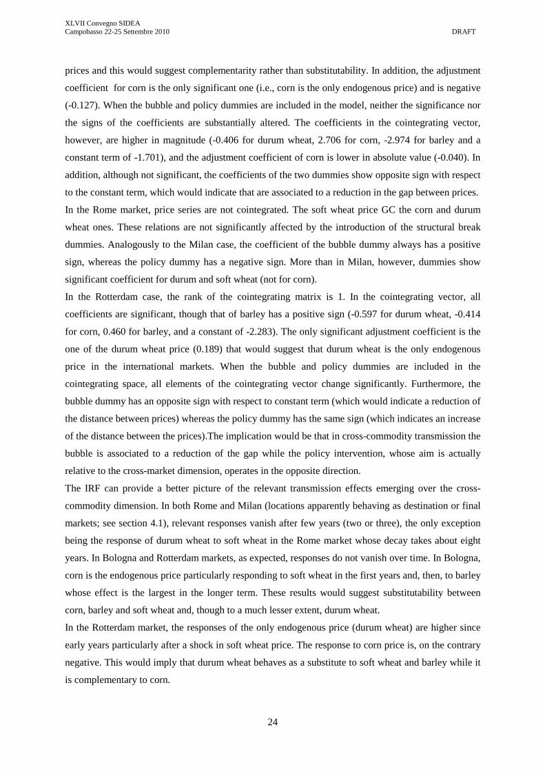
XLVII Convegno SIDEA Campobasso 22-25 Settembre 2010 DRAFT
24
prices and this would suggest complementarity rather than substitutability. In addition, the adjustment
coefficient for corn is the only significant one (i.e., corn is the only endogenous price) and is negative
(-0.127). When the bubble and policy dummies are included in the model, neither the significance nor
the signs of the coefficients are substantially altered. The coefficients in the cointegrating vector,
however, are higher in magnitude (-0.406 for durum wheat, 2.706 for corn, -2.974 for barley and a
constant term of -1.701), and the adjustment coefficient of corn is lower in absolute value (-0.040). In
addition, although not significant, the coefficients of the two dummies show opposite sign with respect
to the constant term, which would indicate that are associated to a reduction in the gap between prices.
In the Rome market, price series are not cointegrated. The soft wheat price GC the corn and durum
wheat ones. These relations are not significantly affected by the introduction of the structural break
dummies. Analogously to the Milan case, the coefficient of the bubble dummy always has a positive
sign, whereas the policy dummy has a negative sign. More than in Milan, however, dummies show
significant coefficient for durum and soft wheat (not for corn).
In the Rotterdam case, the rank of the cointegrating matrix is 1. In the cointegrating vector, all
coefficients are significant, though that of barley has a positive sign (-0.597 for durum wheat, -0.414
for corn, 0.460 for barley, and a constant of -2.283). The only significant adjustment coefficient is the
one of the durum wheat price (0.189) that would suggest that durum wheat is the only endogenous
price in the international markets. When the bubble and policy dummies are included in the
cointegrating space, all elements of the cointegrating vector change significantly. Furthermore, the
bubble dummy has an opposite sign with respect to constant term (which would indicate a reduction of
the distance between prices) whereas the policy dummy has the same sign (which indicates an increase
of the distance between the prices).The implication would be that in cross-commodity transmission the
bubble is associated to a reduction of the gap while the policy intervention, whose aim is actually
relative to the cross-market dimension, operates in the opposite direction.
The IRF can provide a better picture of the relevant transmission effects emerging over the cross-
commodity dimension. In both Rome and Milan (locations apparently behaving as destination or final
markets; see section 4.1), relevant responses vanish after few years (two or three), the only exception
being the response of durum wheat to soft wheat in the Rome market whose decay takes about eight
years. In Bologna and Rotterdam markets, as expected, responses do not vanish over time. In Bologna,
corn is the endogenous price particularly responding to soft wheat in the first years and, then, to barley
whose effect is the largest in the longer term. These results would suggest substitutability between
corn, barley and soft wheat and, though to a much lesser extent, durum wheat.
In the Rotterdam market, the responses of the only endogenous price (durum wheat) are higher since
early years particularly after a shock in soft wheat price. The response to corn price is, on the contrary
negative. This would imply that durum wheat behaves as a substitute to soft wheat and barley while it
is complementary to corn.

XLVII Convegno SIDEA Campobasso 22-25 Settembre 2010 DRAFT
25
5. Concluding remarks
This paper aims at analysing the horizontal transmission (across space and commodities) of
agricultural prices during a period of extreme market turbulence, namely, years 2007-2008. The
proposed methodological approach try to make two different streams of literature converge. On the
one hand, the robust empirical literature on agricultural price linkages based on cointegration analysis
(Listorti, 2009; Carraro and Stefani, 2010). On the other hand, the increasing amount of studies
dealing with explosive behaviour (or bubbles) of financial series or macroeconomic variables
(Nielsen, 2010; Gutierrez, 2010). The novelty of the approach, in fact, consists in analysing the
structural relationships occurring across prices while admitting periods of exuberance during which
such relationships may be affected or a co-explosive relation may overlaps to the conventional
cointegration equation.
The emphasis on the methodological challenges partially left the economic interpretation of results on
the background. In this respect, the empirical evidence here presented has to be regarded as
preliminary and requires a deeper evaluation of implications even from a policy perspective (see
Verga and Zuppiroli, 2003). Nonetheless, even from a strictly methodological point of view some
improvements could be put forward especially trying to emphasize the potential of this kind of
approach and the specific features of agricultural prices and markets.
Methodological developments could start with the estimation of the modified VECM specification
under explosive roots reported in equation (6) (Engsted, 2006; Nielsen, 2010). This would not only
complete the picture by adding also the analysis of the co-explosive relationships; it would also
empirical assess whether estimating the cointegrating relationship within equation (5) or (6) really
provides, in statistical terms, the same outcome. From a different perspective, an improvement in the
investigation of structural price linkages could be achieved by modifying specification (7) by
admitting that structural breaks operate within the cointegration space also affecting price transmission
elasticities (namely, the parameters of the cointegrating vector).
Finally, within the stochastic process describing the cointegrating relationship some further effects
could be included to better mimic the real behavior of agricultural prices especially in periods of
exuberance. On the one hand, co-volatile processes could be included within the price system in the
form of Multiple GARCH models (Yang and Allen, 2005; Tsai and Chen, 2010). On the other hand,
more complex movements within the cointegration space could be introduced, for instance admitting
fractional cointegration (Mohanty et al., 1998) or non-linear cointegration in the form, for instance, of
threshold cointegration or smooth transition cointegration (Mainardi, 2001). All these possible
methodological developments could allow a substantial improvement in the representation of price
linkages over a period of major market exuberance and instability.

XLVII Convegno SIDEA Campobasso 22-25 Settembre 2010 DRAFT
26
References
Ardeni, P.G., 1989. Does the Law of One Price really hold for commodity prices? American
Journal of Agricultural Economics, 71, 661-669.
Benavides, G., 2004. The Theory of Storage and Price Dynamics of Agricultural Commodity Futures:
the Case of Corn and Wheat. Ensayos, XXIX (1), 1-22.
Carraro, A., Stefani, G., 2010. Vertical price transmission in Italian agri-food chains: does the
transmission elasticities change always or sometimes? Paper presented at the XLVII Annual
Conference of the Italian Society of Agricultural Economics (SIDEA), 22-25 September,
Campobasso.
Dawson, P.J., Sanjuan, A., 2006. Structural breaks, the Export Enhancement Program and the
relationship between Canadian and US Hard Wheat prices. Journal of Agricultural Economics, 57
(1), 101-116.
Dawson, P.J., Sanjuan, A.I., White, B., 2006. Structural breaks and the relationship between barley
and wheat future prices on the London international financial futures exchange. Review of
Agricultural Economics, 28 (4), 585-594.
Diba, B., Grossman, H., 1988. Explosive rational bubbles in stock prices. American Economic Review,
78, 520–530.
Ec, 2008. High prices on agricultural commodity markets: situation and prospects. A review of causes
of high prices and outlook for world agricultural markets. European Commission, Directorate
General for Agriculture and Rural Development, Brussels, July.
Enders, W., 1995. Applied Econometric Time Series. New York: John Wiley & Sons.
Engle, R. F., Granger, C. W. J., 1987. Cointegration and error correction: representation, estimation
and testing. Econometrica, 55 (1), 251-276.
Engsted, T., 2006. Explosive bubbles in the cointegrated VAR model. Finance Research Letters, 3 (2),
154-162.
Evans, G.W., 1991. Pitfalls in testing for explosive bubbles in asset prices. American Economic
Review, 81, 922–930.
Fackler, P. L., Goodwin, B. K., 2001. Spatial price analysis. In: B.L. Gardner, G.C. Rausser,
Handbook of Agricultural Economics. Volume 1B. Chapter 17, Amsterdam: Elsevier Science,
972-1025.
Geweke, J., Porter-Hudak, S., 1983. The Estimation and Application of Long Memory Time Series
Models. Journal of Time Series Analysis, 221-238.
Granger, C., Joyeux, R., 1980. An introduction to long memory time series models and fractional
di_erencing. Journal of Time Series Analysis, 1 (1), 15-29.

XLVII Convegno SIDEA Campobasso 22-25 Settembre 2010 DRAFT
27
Gutierrez, L., 2010. Looking for Rational Bubbles in Agricultural Commodity Markets. Paper
presented at the XLVII Annual Conference of the Italian Society of Agricultural Economics
(SIDEA), 22-25 September, Campobasso.
Hamilton, J.D., 1994. Time Series Analysis. 2nd ed. Cambridge, MA: MIT Press.
Irwin S.H., Good D.L., 2009. Market Instability in a New Era of Corn, Soybean, and Wheat Prices.
Choices, 24 (1), pp. 6-11.
Johansen, S., 1991. Cointegration and Hypothesis Testing of Cointegration Vectors in Gaussian
Vector Autoregressive Models. Econometrica, 59 (6), 1551–1580.
Johansen, S., 1995. Maximum Likelihood Inference in Co-Integrated Vector Autoregressive Processes.
Oxford: Oxford University Press.
Johansen, S., Mosconi, R., Nielsen, B., 2000. Cointegration Analysis in the Presence of Structural
Breaks in the Deterministic Trend. The Econometrics Journal, 3, 216–249.
Listorti, G., 2007. Il ruolo delle politiche di mercato dell'UE nei meccanismi internazionali di
trasmissione dei prezzi agricoli: il caso del frumento tenero. Rivista di Economia Agraria, LXII (2),
229-251.
Listorti, G., 2009. Testing International Price Transmission under Policy Intervention. An Application
to the Soft Wheat Market. Associazione Alessandro Bartola. PhD Studies Series, Volume 6.
Mainardi, S. 2001. Limited arbitrage in international wheat markets: threshold and smooth transition
cointegration. Australian Journal of Agricultural and Resource Economics, 45, 335–360.
Mohanty, S. Peterson, E.W.F., Smith, D.B., 1998. Fractional Cointegration and the False Rejection of
the Law of One Price in International Commodity Markets. Journal of Agricultural and Applied
Economics, 30 (2), 267-276.
Nielsen, B., 2010. Analysis of co-explosive processes. Econometric Theory, 26 (3), 882-915.
Pesaran, M.H., 2004. General diagnostic tests for cross section dependence in panels. Cambridge
Working Papers in Economics No. 0435, Faculty of Economics, University of Cambridge.
Phillips, P. C.B., 1999a. Discrete Fourier Transforms of Fractional Processes. Cowles Foundation for
Research in Economics, Discussion Paper No. 1243, Yale University.
Phillips, P.C.B., 1999b. Unit Root Log Periodogram Regression. Cowles Foundation for Research in
Economics, Discussion Paper No. 1244, Yale University.
Phillips, P., Magdalinos, T., 2009. Unit root and cointegrating limit theory when initialization is in the
infinite past. Econometric Theory, 25, 1682–1715.
Phillips, P., Wu, Y., Yu, J., 2009. Explosive behavior in the 1990s Nasdaq: When did exuberance
escalate asset values? Cowles Foundation for Research in Economics, Discussion Paper No. 1699,
Yale University.
Phillips, P., Yu, J., 2009. Dating the timeline of financial bubbles during the subprime crisis. SMU
Economics and Statistics WP series No. 18-2009, Singapore.

XLVII Convegno SIDEA Campobasso 22-25 Settembre 2010 DRAFT
28
Tsai, H-S., Chen, M-C., 2010. The impact of extreme events of dynamics interactions on interest rate,
real house price and stock markets”. International Research Journal of Finance and Economics,
35, 187-201.
Verga, G., Zuppiroli, M., 2003. Integrazione e causalità nel mercato europeo del frumento tenero.
Rivista di Economia Agraria, LVIII (3), 323-364.
Wei A., Leuthold, R.M., 1998. Long Agricultural Future Prices: ARCH, Long Memory or Chaos
Processes? OFOR Paper n. 98-03, Department of Agricultural Economics, University of Illinois at
Urbana-Champaign.
Wright, B., 2001. Storage and Price Stabilization. In: B.L. Gardner, G.C. Rausser, Handbook of
Agricultural Economics. Volume 1B. Chapter 14, Amsterdam: Elsevier Science, 817-861.
Yang, W., Allen, D. E., 2005. Multivariate GARCH hedge ratios and hedging effectiveness in
Australian futures markets. Accounting & Finance, 45, 301–321.
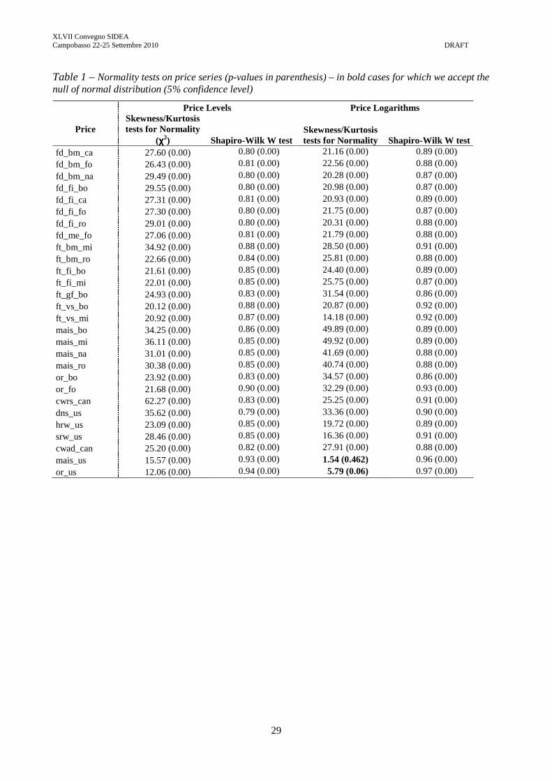
XLVII Convegno SIDEA Campobasso 22-25 Settembre 2010 DRAFT
29
Table 1 – Normality tests on price series (p-values in parenthesis) – in bold cases for which we accept the null of normal distribution (5% confidence level)
Price Levels Price Logarithms
Price Skewness/Kurtosis tests for Normality
(χχχχ2) Shapiro-Wilk W test Skewness/Kurtosis tests for Normality Shapiro-Wilk W test
fd_bm_ca 27.60 (0.00) 0.80 (0.00) 21.16 (0.00) 0.89 (0.00)
fd_bm_fo 26.43 (0.00) 0.81 (0.00) 22.56 (0.00) 0.88 (0.00)
fd_bm_na 29.49 (0.00) 0.80 (0.00) 20.28 (0.00) 0.87 (0.00)
fd_fi_bo 29.55 (0.00) 0.80 (0.00) 20.98 (0.00) 0.87 (0.00)
fd_fi_ca 27.31 (0.00) 0.81 (0.00) 20.93 (0.00) 0.89 (0.00)
fd_fi_fo 27.30 (0.00) 0.80 (0.00) 21.75 (0.00) 0.87 (0.00)
fd_fi_ro 29.01 (0.00) 0.80 (0.00) 20.31 (0.00) 0.88 (0.00)
fd_me_fo 27.06 (0.00) 0.81 (0.00) 21.79 (0.00) 0.88 (0.00)
ft_bm_mi 34.92 (0.00) 0.88 (0.00) 28.50 (0.00) 0.91 (0.00)
ft_bm_ro 22.66 (0.00) 0.84 (0.00) 25.81 (0.00) 0.88 (0.00)
ft_fi_bo 21.61 (0.00) 0.85 (0.00) 24.40 (0.00) 0.89 (0.00)
ft_fi_mi 22.01 (0.00) 0.85 (0.00) 25.75 (0.00) 0.87 (0.00)
ft_gf_bo 24.93 (0.00) 0.83 (0.00) 31.54 (0.00) 0.86 (0.00)
ft_vs_bo 20.12 (0.00) 0.88 (0.00) 20.87 (0.00) 0.92 (0.00)
ft_vs_mi 20.92 (0.00) 0.87 (0.00) 14.18 (0.00) 0.92 (0.00)
mais_bo 34.25 (0.00) 0.86 (0.00) 49.89 (0.00) 0.89 (0.00)
mais_mi 36.11 (0.00) 0.85 (0.00) 49.92 (0.00) 0.89 (0.00)
mais_na 31.01 (0.00) 0.85 (0.00) 41.69 (0.00) 0.88 (0.00)
mais_ro 30.38 (0.00) 0.85 (0.00) 40.74 (0.00) 0.88 (0.00)
or_bo 23.92 (0.00) 0.83 (0.00) 34.57 (0.00) 0.86 (0.00)
or_fo 21.68 (0.00) 0.90 (0.00) 32.29 (0.00) 0.93 (0.00)
cwrs_can 62.27 (0.00) 0.83 (0.00) 25.25 (0.00) 0.91 (0.00)
dns_us 35.62 (0.00) 0.79 (0.00) 33.36 (0.00) 0.90 (0.00)
hrw_us 23.09 (0.00) 0.85 (0.00) 19.72 (0.00) 0.89 (0.00)
srw_us 28.46 (0.00) 0.85 (0.00) 16.36 (0.00) 0.91 (0.00)
cwad_can 25.20 (0.00) 0.82 (0.00) 27.91 (0.00) 0.88 (0.00)
mais_us 15.57 (0.00) 0.93 (0.00) 1.54 (0.462) 0.96 (0.00)
or_us 12.06 (0.00) 0.94 (0.00) 5.79 (0.06) 0.97 (0.00)

XLVII Convegno SIDEA Campobasso 22-25 Settembre 2010 DRAFT
30
Table 2 – Structure of autocorrelations: evidence from partial autocorrelogram (PAC)
Price Levels Price Logarithms
Price Highest PAC term
At lag
Latest consecutive
lag with significant
PCa
Other significant
lagsa,b
Highest PAC term
At lag
Latest consecutive
lag with significant
PCa
Other significant
lagsa,b
fd_bm_ca 0.996 1 4 6, 9, 12, 17, 31,
34 (+), 35 (+), 46, 49
0.996 1 4 17, 35 (+)
fd_bm_fo 0.997 1 3 6, 16, 29, 39 (+), 47, 50 0.997 1 3 6, 16, 47
fd_bm_na 0.997 1 2 5, 10, 34 (+), 49, 50 (-) 0.997 1 2 5, 10, 12, 49, 50 (-
)
fd_fi_bo 0.998 1 4 19, 33 (+), 34 0.998 1 4 19, 33 (+), 34, 51
fd_fi_ca 0.996 1 4 6, 9, 12, 17, 34 (+), 35 (+), 46 0.996 1 4 4, 17, 35 (+)
fd_fi_fo 0.997 1 2 6, 11, 16 0.997 1 2 6, 11, 12, 19, 26, 36, 47
fd_fi_ro 0.998 1 4 8, 11, 15, 49 0.998 1 4 11, 46
fd_me_fo 0.997 1 3 6, 28 (+), 29 (+), 50 0.997 1 3 6, 16, 26, 34, 47
ft_bm_mi 0.993 1 3 48 0.992 1 3 48
ft_bm_ro 0.997 1 2 11, 16 (+), 18, 22, 48, 50(+) 0.997 1 2 8 (+), 11, 16 (+),
18, 48, 50(+)
ft_fi_bo 0.995 1 3 11, 17 (+), 20, 32 0.995 1 3 8 (+), 11, 20, 32
ft_fi_mi 0.992 1 2 - 0.989 1 2 -
ft_gf_bo 0.996 1 2 18, 19 (+), 20, 25, 32, 48 0.996 1 2 19 (+), 20, 37, 48
ft_vs_bo 0.994 1 2 11, 18, 19 (+), 20, 48 0.993 1 2 20, 48
ft_vs_mi 0.991 1 2 5, 29, 47 0.989 1 2 29, 47
mais_bo 0.991 1 2 4, 8 (+), 9 (+), 42, 43 0.991 1 2 4, 8 (+), 9 (+), 19,
42, 43
mais_mi 0.992 1 2 4, 8 (+), 12, 42, 47 0.992 1 2 4, 5, 8 (+), 42, 47
mais_na 0.988 1 2 6, 9 (+), 25, 29, 35 (+), 42, 46, 47 0.988 1 2
6, 9 (+), 25, 26, 35 (+), 36 (+), 42,
46, 47, 48
mais_ro 0.983 1 2 4, 8 (+), 26, 43, 44, 49 0.984 1 2 4, 6, 8 (+), 43, 49
or_bo 0.998 1 2 4, 7, 8 (+), 20, 22, 36 (+), 40, 49 0.997 1 2 7, 8 (+), 20, 22,
36 (+), 40
or_fo 0.995 1 2 4, 14, 15, 27, 29, 40 0.994 1 2 4, 15, 27, 29, 40
cwrs_can 0.977 1 1 3, 5(+), 9, 10 (+), 13, 22 (+), 23, 29, 31 (+), 41, 46 (+)
0.982 1 1 3, 5(+), 9, 10 (+), 13, 23, 29, 41
dns_us 0.978 1 2 5, 8 (+), 14 (+) 0.978 1 2 8, 35 (+), 48
hrw_us 0.982 1 1 3, 7 (+), 9, 28, 29 0.983 1 1 3, 9, 49
srw_us 0.981 1 1 3, 9, 25, 28, 32 (+) 0.979 1 1 3, 32 (+), 35 (+),
43, 48, 49, 50 (+)
cwad_can 0.993 1 2 10, 12, 15, 17, 18, 29 (+), 48 0.993 1 1
3, 4, 5, 15, 20, 27 (+), 35, 39(+) , 44, 46 (+), 48, 49, 50
mais_us 0.970 1 1 3, 6 (+), 11, 22, 33, 34, 51 0.967 1 1 3, 34, 40, 46 (+),
47 (+), 49, 52
or_us 0.984 1 2 4, 12, 45, 48 0.979 1 2 4, 12, 45, 47 a 95% confidence bands b In parenthesis the sign of the significant partial correlation term

XLVII Convegno SIDEA Campobasso 22-25 Settembre 2010 DRAFT
31
Table 3 – Adjusted Dickey-Fuller (ADF) and Phillips-Perron (PP) unit root tests on price series (H0: unit root; p-values in parenthesis)a – in bold cases for which the null is rejected (5% confidence level)
Price Levels Price Logarithms ∆ Price Levels ∆ Price Logarithms Price
ADF PP ADF PP ADF PP ADF PP
fd_bm_ca -1.647 (0.458)
-1.364 (0.599)
-1.646 (0.459)
-1.345 (0.608)
-2.501 (0.115)
-6.492 (0.000)
-2.497 (0.116)
-6.553 (0.000)
fd_bm_fo -1.321 (0.622)
-1.287 (0.635)
-1.424 (0.572)
-1.235 (0.658)
-3.840 (0.002)
-7.296 (0.000)
-3.114 (0.026)
-7.440 (0.000)
fd_bm_na -1.639 (0.462)
-1.274 (0.641)
-1.585 (0.49)
-1.160 (0.690)
-3.270 (0.016)
-6.157 (0.000)
-3.423 (0.010)
-6.730 (0.000)
fd_fi_bo 1.796 (0.383)
-1.251 (0.651)
-1.075 (0.728)
-1.112 (0.710)
-4.619 (0.000)
-5.773 (0.000)
-5.428 (0.000)
-6.501 (0.000)
fd_fi_ca -1.646 (0.459)
-1.371 (0.596)
-1.640 (0.462)
-1.353 (0.604)
-2.532 (0.108)
-6.538 (0.000)
-3.808 (0.003)
-6.615 (0.000)
fd_fi_fo -1.902 (0.331)
-1.292 (0.633)
-1.887 (0.339)
-1.226 (0.662)
-2.096 (0.246)
-5.465 (0.000)
-2.128 (0.234)
-6.616 (0.000)
fd_fi_ro -2.026 (0.276)
-1.264 (0.646)
-1.909 (0.328)
-1.124 (0.705)
-1.914 (0.326)
-5.810 (0.000)
-2.005 (0.285)
-6.218 (0.000)
fd_me_fo -1.501 (0.533)
-1.298 (0.630)
-1.448 (0.560)
-1.238 (0.657)
-3.986 (0.001)
-6.570 (0.000)
-3.094 (0.027)
-7.160 (0.000)
ft_bm_mi -1.157 (0.695)
-1.405 (0.580)
-1.172 (0.689)
-1.471 (0.548)
-5.426 (0.000)
-10.079 (0.000)
-5.895 (0.000)
-10.678 (0.000)
ft_bm_ro -1.366 (0.600)
-1.261 (0.647)
-1.638 (0.463)
-1.254 (0.650)
-3.400 (0.011)
-6.088 (0.000)
-2.944 (0.040)
-6.014 (0.000)
ft_fi_bo -1.640 (0.461)
-1.323 (0.619)
-1.312 (0.626)
-1.335 (0.613)
-2.423 (0.135)
-7.837 (0.000)
-3.664 (0.005)
-7.670 (0.000)
ft_fi_mi -1.022 (0.748)
-1.396 (0.584)
-1.006 (0.753)
-1.464 (0.551)
-6.730 (0.000)
-12.649 (0.000)
-10.727 (0.000)
-13.004 (0.000)
ft_gf_bo -1.382 (0.593)
-1.273 (0.641)
-1.401 (0.583)
-1.253 (0.650)
-5.771 (0.000)
-6.661 (0.000)
-3.413 (0.010)
-6.675 (0.000)
ft_vs_bo -1.610 (0.477)
-1.450 (0.558)
-1.463 (0.553)
-1.511 (0.528)
-5.832 (0.000)
6.861 (0.000)
-3.422 (0.010)
-6.884 (0.000)
ft_vs_mi -1.315 (0.625)
-1.529 (0.519)
-1.224 (0.666)
-1.621 (0.472)
-8.812 (0.000)
-11.463 (0.000)
-9.072 (0.000)
-11.560 (0.000)
mais_bo -1.498 (0.535)
-1.612 (0.477)
-1.534 (0.516)
-1.656 (0.454)
-4.442 (0001)
-7.746 (0.000)
-2.595 (0.094)
-7.619 (0.000)
mais_mi -1.433 (0.568)
-1.571 (0.498)
-1.534 (0.516)
-1.615 (0.475)
-3.030 (0.032)
-9.131 (0.000)
-3.545 (0.007)
-8.694 (0.000)
mais_na -1.364 (0.601)
-1.664 (0.450)
-1.437 (0.565)
-1.726 (0.418)
-3.953 (0.012)
-10.134 (0.000)
-3.784 (0.003)
-10.362 (0.000)
mais_ro -1.586 (0.490)
-1.749 (0.406)
-1.616 (0.474)
-1.815 (0.373)
-2.754 (0.065)
-11.786 (0.000)
-2.704 (0.073)
-11.388 (0.000)
or_bo -1.659 (0.452)
-1.164 (0.689)
-1.618 (0.473)
-1.142 (0.698)
-2.328 (0.163)
-7.034 (0.000)
-2.603 (0.092)
-7.149 (0.000)
or_fo -1.208 (0.673)
-1.300 (0.629)
-1.201 (0.677)
-1.320 (0.620)
-4.090 (0.001)
-9.911 (0.000)
-4.198 (0.001)
-11.003 (0.000)
cwrs_can -1.323 (0.621)
-1.831 (0.365)
-1.317 (0.624)
-1.699 (0.432)
-3.443 (0.010)
-13.301 (0.000)
-3.315 (0.014)
-13.945 (0.000)
dns_us -1.496 (0.536)
-1.960 (0.304)
-1.499 (0.534)
-1.794 (0.384)
-3.635 (0.005)
-8.169 (0.000)
-9.065 (0.000)
-10.815 (0.000)
hrw_us -1.189 (0.682)
-1.539 (0.514)
-1.099 (0.719)
-1.556 (0.505)
3.740 (0.004)
-15.105 (0.000)
-7.319 (0.000)
-15.177 (0.000)
srw_us -1.443 (0.563)
-1.754 (0.403)
-1.304 (0.630)
-1.869 (0.346)
-5.517 (0.000)
-15.003 (0.000)
-7.529 (0.000)
-15.265 (0.000)
cwad_can -1.639 (0.462)
-1.376 (0.594)
-1.067 (0.731)
-1.374 (0.595)
-2.193 (0.209)
-10.484 (0.000)
-4.794 (0.000)
-14.008 (0.000)
mais_us -2.165 (0.219)
-2.167 (0.218)
-2.234 (0.194)
-2.399 (0.142)
-2.881 (0.047)
-13.819 (0.000)
-2.487 (0.118)
-15.302 (0.000)
or_us -1.864 (0.350)
-2.007 (0.283)
-1.952 (0.308)
-2.198 (0.207)
-2.790 (0.060)
-11.451 (0.000)
-2.902 (0.045)
-12.076 (0.000)
a The ADF test specification includes a constant term, all significant lags “testing down” up to a maximum of 12, and seasonal dummies. The ADF tests have been repeated also without the inclusion of a constant term, and, both with and without the constant term, without seasonal dummies. Phillips-Perron tests have been repeated with 4 lags (number determined with the Newey-West procedure) and 12 lags, in both cases with and without the inclusion of a constant term. The table shows the results of the specification with 12 lags and a constant term. Results do not substantially differ between the various test specifications.

XLVII Convegno SIDEA Campobasso 22-25 Settembre 2010 DRAFT
32
Table 4 – ARCH(p) tests on ADF unit-root test equations (Table 3) (H0: no ARCH effects; ; p-values in parenthesis) a – in bold cases for which the null is rejected (5% confidence level)
Price Price Levels Price Logarithms
fd_bm_ca 2.608 (0.998) 1.197 (0.000) fd_bm_fo 19.948 (0.068) 9.634 (0.648) fd_bm_na 20.158 (0.064) 28.039 (0.006) fd_fi_bo 2.221 (0.999) 10.926 (0.535) fd_fi_ca 2.921 (0.996) 1.342 (0.999) fd_fi_fo 33.927 (0.000) 18.447 (0.103) fd_fi_ro 4.547 (0.971) 14.217 (0.287) fd_me_fo 13.816 (0.313) 8.946 (0.708) ft_bm_mi 2.767 (0.997) 1.317 (0.999) ft_bm_ro 27.788 (0.006) 15.153 (0.233) ft_fi_bo 29.041 (0.004) 16.882 (0.154) ft_fi_mi 0.338 (1.000) 0.179 (1.000) ft_gf_bo 10.149 (0.603) 12.071 (0.440) ft_vs_bo 13.252 (0.351) 11.223 (0.509) ft_vs_mi 0.465 (1.000) 0.226 (1.000) mais_bo 28.373 (0.005) 28.679 (0.004) mais_mi 17.056 (0.148) 17.996 (0.116) mais_na 27.526 (0.006) 22.184 (0.036) mais_ro 11.845 (0.458) 10.808 (0.546) or_bo 7.771 (0.803) 7.820 (0.799) or_fo 19.289 (0.082) 19.825 (0.071) cwrs_can 5.468 (0.940) 15.092 (0.236) dns_us 17.211 (0.142) 13.111 (0.361) hrw_us 38.874 (0.000) 22.648 (0.031) srw_us 38.180 (0.000) 12.490 (0.442) cwad_can 36.585 (0.000) 39.491 (0.000) mais_us 42.016 (0.000) 21.949 (0.038) or_us 7.603 (0.815) 7.620 (0.814)
a The ARCH test is an LM test, thus is distributed as a χ2(p). The adopted specification includes 12 lags (p=12)

XLVII Convegno SIDEA Campobasso 22-25 Settembre 2010 DRAFT
33
Table 5 – Long-memory tests p-values: test of fractional integration of the price series according to Phillips (1999a,b). If d=0 the series is I(1); if d=1 the series is I(1); if 0<d<1, the series is I(d)(long memory process) a – in bold cases for which the null is accepted (5% confidence level)
Price Levels Price Logarithms ∆ Price Levels ∆ Price Logarithms
Price t (H0: d=0) z (H0: d=1) t (H0: d=0) z (H0: d=1) t (H0: d=0) z (H0: d=1) t (H0: d=0) z (H0: d=1)
fd_bm_ca 0.000 0.110 0.000 0.098 0.186 0.000 0.028 0.000 fd_bm_fo 0.000 0.061 0.000 0.119 0.264 0.000 0.146 0.000 fd_bm_na 0.000 0.087 0.000 0.140 0.039 0.000 0.078 0.000 fd_fi_bo 0.000 0.047 0.000 0.117 0.031 0.000 0.029 0.000 fd_fi_ca 0.000 0.108 0.000 0.098 0.227 0.000 0.040 0.000 fd_fi_fo 0.000 0.068 0.000 0.118 0.140 0.000 0.134 0.000 fd_fi_ro 0.000 0.046 0.000 0.092 0.001 0.000 0.014 0.000 fd_me_fo 0.000 0.066 0.000 0.124 0.323 0.000 0.274 0.000 ft_bm_mi 0.000 0.085 0.000 0.068 0.049 0.000 0.144 0.000 ft_bm_ro 0.000 0.004 0.000 0.000 0.054 0.000 0.015 0.000 ft_fi_bo 0.000 0.249 0.000 0.115 0.204 0.000 0.077 0.000 ft_fi_mi 0.000 0.204 0.000 0.148 0.231 0.000 0.423 0.000 ft_gf_bo 0.000 0.341 0.000 0.194 0.219 0.000 0.121 0.000 ft_vs_bo 0.000 0.377 0.000 0.193 0.224 0.000 0.101 0.000 ft_vs_mi 0.000 0.067 0.000 0.007 0.059 0.000 0.016 0.000 mais_bo 0.000 0.056 0.000 0.017 0.100 0.000 0.089 0.000 mais_mi 0.000 0.022 0.000 0.082 0.029 0.000 0.020 0.000 mais_na 0.002 0.875 0.000 0.689 0.244 0.000 0.155 0.000 mais_ro 0.000 0.688 0.000 0.389 0.137 0.000 0.100 0.000 or_bo 0.000 0.002 0.000 0.010 0.000 0.006 0.003 0.000 or_fo 0.000 0.652 0.000 0.134 0.137 0.000 0.130 0.000 cwrs_can 0.000 0.833 0.000 0.105 0.636 0.000 0.629 0.000 dns_us 0.000 0.300 0.000 0.490 0.023 0.000 0.919 0.000 hrw_us 0.000 0.604 0.000 0.331 0.835 0.000 0.536 0.000 srw_us 0.000 0.167 0.000 0.162 0.266 0.000 0.103 0.000 cwad_can 0.000 0.035 0.000 0.022 0.095 0.000 0.052 0.000 mais_us 0.000 0.995 0.000 0.749 0.900 0.000 0.510 0.000 or_us 0.001 0.895 0.000 0.482 0.936 0.000 0.836 0.000
a As a deterministic trend has been excluded the original test has not been detrended. The test run under alternative possible values of the arbitrary power parameter here assumed equal to 0.5521
21 Test robustness is often assessed using a set of values of the power parameter (see Phillips, 1999a,b) ranging from 0.4 to 0.75. Here, a value in the middle of this range has been adopted. Nonetheless, test results for alternative values of the power parameter have been also obtained and are available on request. They do not significantly differ, however, from those here presented.
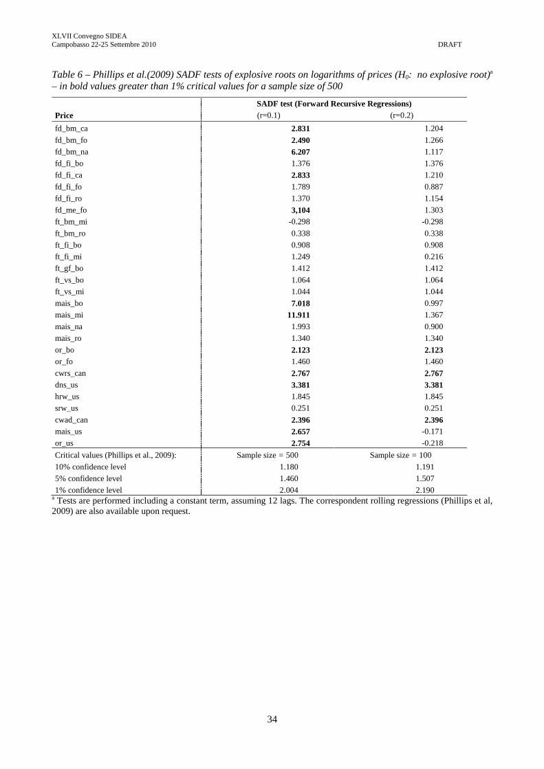
XLVII Convegno SIDEA Campobasso 22-25 Settembre 2010 DRAFT
34
Table 6 – Phillips et al.(2009) SADF tests of explosive roots on logarithms of prices (H0: no explosive root)a
– in bold values greater than 1% critical values for a sample size of 500
SADF test (Forward Recursive Regressions) Price (r=0.1) (r=0.2)
fd_bm_ca 2.831 1.204
fd_bm_fo 2.490 1.266 fd_bm_na 6.207 1.117 fd_fi_bo 1.376 1.376 fd_fi_ca 2.833 1.210
fd_fi_fo 1.789 0.887
fd_fi_ro 1.370 1.154
fd_me_fo 3,104 1.303
ft_bm_mi -0.298 -0.298 ft_bm_ro 0.338 0.338 ft_fi_bo 0.908 0.908 ft_fi_mi 1.249 0.216 ft_gf_bo 1.412 1.412 ft_vs_bo 1.064 1.064 ft_vs_mi 1.044 1.044 mais_bo 7.018 0.997
mais_mi 11.911 1.367 mais_na 1.993 0.900 mais_ro 1.340 1.340 or_bo 2.123 2.123 or_fo 1.460 1.460
cwrs_can 2.767 2.767 dns_us 3.381 3.381 hrw_us 1.845 1.845
srw_us 0.251 0.251
cwad_can 2.396 2.396 mais_us 2.657 -0.171
or_us 2.754 -0.218
Critical values (Phillips et al., 2009): Sample size = 500 Sample size = 100 10% confidence level 1.180 1.191
5% confidence level 1.460 1.507
1% confidence level 2.004 2.190 a Tests are performed including a constant term, assuming 12 lags. The correspondent rolling regressions (Phillips et al, 2009) are also available upon request.

XLVII Convegno SIDEA Campobasso 22-25 Settembre 2010 DRAFT
35
Table 7 – Matrix of correlation coefficients across price series
fd_bm_ca fd_bm_fo fd_bm_na fd_fi_bo fd_fi_ca fd_fi_fo fd_fi_ro fd_me_fo ft_bm_mi ft_bm_ro ft_fi_bo ft_fi_mi ft_gf_bo ft_vs_bo ft_vs_mi mais_bo mais_mi mais_na mais_ro or_bo or_fo cwrs_can dns_us hrw_us srw_us cwad_can mais_us or_usfd_bm_ca 1 0.9938 0.9947 0.9925 0.9999 0.9948 0.9949 0.9937 0.9103 0.9359 0.9089 0.8915 0.938 0.9225 0.94 0.8166 0.8366 0.8489 0.8434 0.8764 0.9161 0.9054 0.8704 0.9376 0.9036 0.9738 0.7727 0.8347fd_bm_fo 1 0.9949 0.9952 0.994 0.9988 0.9961 0.9997 0.9095 0.9396 0.9114 0.8901 0.9374 0.9187 0.936 0.8396 0.8584 0.8666 0.8651 0.8814 0.9089 0.8981 0.8683 0.9414 0.9024 0.9673 0.7812 0.8288fd_bm_na 1 0.9967 0.9946 0.9968 0.9977 0.9947 0.9161 0.9421 0.9153 0.8975 0.9407 0.9266 0.9449 0.8241 0.8421 0.8516 0.8458 0.8848 0.918 0.9123 0.8788 0.9422 0.912 0.9723 0.7586 0.8235fd_fi_bo 1 0.9925 0.9975 0.9981 0.9949 0.9133 0.9475 0.9227 0.8881 0.9441 0.9276 0.9467 0.8401 0.8564 0.864 0.8606 0.8962 0.9128 0.8994 0.8661 0.939 0.9163 0.964 0.7475 0.8295fd_fi_ca 1 0.9949 0.995 0.9939 0.9074 0.9337 0.9063 0.8883 0.9356 0.9201 0.9391 0.8135 0.8334 0.8461 0.8413 0.8729 0.9114 0.9052 0.8703 0.9366 0.9015 0.9732 0.7714 0.8327fd_fi_fo 1 0.9972 0.9983 0.9148 0.9458 0.9189 0.8931 0.9435 0.9263 0.9425 0.8395 0.8577 0.8673 0.8653 0.8901 0.9134 0.897 0.8644 0.9406 0.9113 0.9665 0.7682 0.8352fd_fi_ro 1 0.9958 0.9129 0.9414 0.9154 0.8916 0.9386 0.9242 0.945 0.8285 0.8454 0.8543 0.8491 0.8848 0.9148 0.9066 0.8731 0.9388 0.9066 0.9674 0.7558 0.8214fd_me_fo 1 0.9057 0.9359 0.9073 0.886 0.9327 0.9141 0.9323 0.8355 0.8543 0.8627 0.8608 0.8781 0.9045 0.8974 0.8675 0.9383 0.8986 0.9667 0.7803 0.8235ft_bm_mi 1 0.9685 0.9625 0.9876 0.9753 0.9828 0.9185 0.8606 0.8739 0.8755 0.8778 0.9232 0.9428 0.8089 0.7639 0.9037 0.9033 0.9052 0.753 0.8889ft_bm_ro 1 0.9932 0.9322 0.9874 0.9859 0.969 0.9239 0.9336 0.938 0.9371 0.9694 0.9393 0.8277 0.7849 0.9371 0.9501 0.9133 0.749 0.9209ft_fi_bo 1 0.9183 0.9802 0.9855 0.962 0.9349 0.9399 0.9438 0.9383 0.98 0.932 0.7997 0.7573 0.9192 0.9495 0.8828 0.7288 0.9256ft_fi_mi 1 0.9518 0.9563 0.8758 0.8034 0.8215 0.8219 0.8278 0.8646 0.9358 0.8075 0.7611 0.891 0.8615 0.906 0.7628 0.8501ft_gf_bo 1 0.9923 0.9571 0.8904 0.9042 0.9069 0.9088 0.9417 0.9505 0.8363 0.796 0.9406 0.9465 0.9275 0.7666 0.9237ft_vs_bo 1 0.9616 0.8843 0.8933 0.9002 0.899 0.9427 0.9431 0.8273 0.7825 0.9268 0.9449 0.9133 0.7576 0.9294ft_vs_mi 1 0.8831 0.8885 0.9011 0.8885 0.9348 0.9152 0.8725 0.8376 0.9295 0.9498 0.9169 0.7573 0.9014mais_bo 1 0.9963 0.9874 0.9783 0.9526 0.8537 0.7087 0.6886 0.8508 0.8823 0.7781 0.7257 0.8705mais_mi 1 0.9913 0.9838 0.9563 0.873 0.7255 0.7044 0.8658 0.8891 0.7997 0.7405 0.8796mais_na 1 0.9895 0.957 0.8743 0.7383 0.7092 0.8696 0.9017 0.8087 0.7344 0.8913mais_ro 1 0.9435 0.8556 0.7129 0.6811 0.8642 0.8879 0.8036 0.722 0.8913or_bo 1 0.9158 0.7581 0.7178 0.8728 0.9255 0.8312 0.6805 0.8889or_fo 1 0.8486 0.806 0.9084 0.9003 0.9117 0.7512 0.8578cwrs_can 1 0.9809 0.9225 0.8758 0.9394 0.7538 0.7159dns_us 1 0.8956 0.8445 0.9118 0.7479 0.6737hrw_us 1 0.9515 0.9606 0.8013 0.8635srw_us 1 0.9068 0.7308 0.9062cwad_can 1 0.7909 0.828mais_us 1 0.7811or_us 1

XLVII Convegno SIDEA Campobasso 22-25 Settembre 2010 DRAFT
36
Table 8A – Cross-market commodity price linkage: VECM estimates (standard errors in parenthesis) – durum wheat, national prices a Trace (Johansen) test
Rank = 0 43.36
Rank = 1 13.23†
Rank = 2 1.52
Rank = 3 -
Cointegrating vector (β) Without breaks With breaks Bologna 1.000 1.000 Rome -0.235 (0.126) -0.211 (0.132)
Foggia -0.811* (0.127) -0.882* (0.139)
bubble dummy 0.0247 (0.020)
policy dummy 0.026 (0.017)
Constant 0.254* (0.056) 0.507* (0.142)
Adjustment vector (α) Bologna -0.037 (0.073) -0.002 (0.073)
Rome 0.059 (0.058) 0.091 (0.058)
Foggia 0.211* (0.060) 0.222* (0.059)
ADF test on long-run residualsb -2.882* -5.20* a Estimated coefficients of the adjustment vectors (α) and of the first-difference terms are available upon request. The optimal lag of the VECM has been selected according to the conventional information criteria. Whereas the HQIC and SBIC indicated 2 lags, 3 lags, as indicated by the AIC, were necessary in order to remove autocorrelation in the residuals of the VECM (LM test up to the 4th lag). b ADF test specification includes 12 lags †Accepted rank: lowest rank whose test result is lower than 5% critical values *Statistically significant at 5% confidence level Table 8B – Cross-market commodity price linkage: VECM estimates (standard errors in parenthesis) – durum wheat, national and international prices a Trace (Johansen) test
Rank = 0 57.58
Rank = 1 22.35†
Rank = 2 7.29
Rank = 3 1.89
Rank = 4 -
Cointegrating vector (β) Without breaks With breaks Bologna 1.000 1.000
Rome -0.472* (0.110) -0.468* (0.120)
Foggia -0.648* (0.103) -0.697* (0.115)
Rotterdam 0.069* (0.026) 0.086* (0.029)
bubble dummy 0.014 (0.016)
policy dummy 0.007 (0.014)
Constant 0.264* (0.046) 0.407* (0.117)
Adjustment vector (α) Bologna -0.003 (0.083) 0.0299 (0.083)
Rome 0.134* (0.066) 0.1509* (0.065)
Foggia 0.256* (0.069) 0.273* (0.067)
Rotterdam 0.081 (0.156) 0.064 (0.1557)
ADF test on long-run residualsb 2.863* -3.64* a Estimated coefficients of the adjustment vectors (α) and of the first-difference terms are available upon request. The optimal lag of the VECM has been selected according to the conventional information criteria. Whereas the HQIC and SBIC indicated 2 lags, 3 lags, as indicated by the AIC, were necessary in order to remove autocorrelation in the residuals of the VECM (LM test up to the 4th lag). b The ADF test specification includes 12 lags †Accepted rank: lowest rank whose test result is lower than 5% critical values *Statistically significant at 5% confidence level

XLVII Convegno SIDEA Campobasso 22-25 Settembre 2010 DRAFT
37
Table 8C – Cross-market commodity price linkage: first-difference VAR estimates – High quality soft wheat, national prices a Trace (Johansen) test
Rank = 0 8.54†
Rank = 1 2.43
Rank = 2 -
Short-run Granger Causality tests (χ2) Without breaks With breaks Bologna on Milan 33.24* 26.89*
Milan on Bologna 2.78 1.61
VAR coefficients
Milan: bubble dummy - 0.007
policy dummy - -0.011*
Bologna: bubble dummy - 0.003
policy dummy - -0.004
ADF test on residualsb
Milan -3.68* -4.39*
Bologna -3.50* -3.91* a The other estimated coefficients of the VAR are available upon request. The optimal lag of the VECM has been selected according to the conventional information criteria. 2 lags in the levels of the variables and 1 in their differences, as indicated by HQIC, SBIC and AIC, were sufficient in order to remove autocorrelation in the residuals of the VAR (LM test up to the 4th lag). A constant terms is included in VAR equations b The ADF test specification includes 12 lags †Accepted rank: lowest rank whose test result is lower than 5% critical values *Statistically significant at 5% confidence level Table 8D – Cross-market commodity price linkage: first-difference VAR estimates – High quality soft wheat, national and international prices a Trace (Johansen) test
Rank = 0 21.93†
Rank = 1 10.12
Rank = 2 2.13
Rank = 3 -
Short-run Granger Causality tests (χ2) Without breaks With breaks Bologna on Milan 22.88* 18.92*
US on Milan 16.07* 14.52*
Milan on Bologna 3.04 1.88
US on Bologna 4.61* 3.93*
Milan on US 5.06* 3.20
Bologna on US 0.03 0.05
VAR coefficients
Milan: bubble dummy - 0.006
policy dummy - -0.009*
Bologna: bubble dummy - 0.003
policy dummy - -0.004
US: bubble dummy - 0.012
policy dummy - -0.012
ADF test on residualsb
Milan -3.64* -4.22*
Bologna -3.68* -4.02*
US -3.25* -3.87* a The other estimated coefficients of the VAR are available upon request. The optimal lag of the VECM has been selected according to the conventional information criteria. 2 lags in the levels of the variables and 1 in their differences, as indicated by HQIC, SBIC and AIC, were sufficient in order to remove autocorrelation in the residuals of the VAR (LM test up to the 4th lag). A constant terms in included in VAR equations b The ADF test specification includes 12 lags †Accepted rank: lowest rank whose test result is lower than 5% critical values *Statistically significant at 5% confidence level

XLVII Convegno SIDEA Campobasso 22-25 Settembre 2010 DRAFT
38
Table 8E – Cross-market commodity price linkage: first-difference VAR estimates – Medium quality soft wheat, national prices a Trace (Johansen) test
Rank = 0 16.35†
Rank = 1 2.44
Rank = 2 -
Short-run Granger Causality tests (χ2) Without breaks With breaks Bologna on Milan 20.31* 17.61*
Milan on Bologna 2.70 2.68
VAR coefficients
Milan: bubble dummy - 0.005
policy dummy - 0.003
Bologna: bubble dummy - 0.004
policy dummy - -0.007*
ADF test on residualsb
Milan -3.93* -3.90*
Bologna -3.18* -3.75* a The other estimated coefficients of the VAR are available upon request. The optimal lag of the VECM has been selected according to the conventional information criteria. 2 lags in the levels of the variables and 1 in their differences were indicated by HQIC and SBIC; 3 lags in the levels and 2 in the differences, as indicated by the AIC, were preferred as they allow to remove autocorrelation in the residuals (LM test up to the 4th lag). A constant terms in included in VAR equations. b The ADF test specification includes 12 lags †Accepted rank: lowest rank whose test result is lower than 5% critical values *Statistically significant at 5% confidence level Table 8F – Cross-market commodity price linkage: first-difference VAR estimates – Medium quality soft wheat, national and international prices a Trace (Johansen) test
Rank = 0 28.04†
Rank = 1 12.79
Rank = 2 3.23
Rank = 3 -
Short-run Granger Causality tests (χ2) Without breaks With breaks Bologna on Milan 20.05* 17.46*
US on Milan 0.01 0.01
Milan on Bologna 1.04 1.15
US on Bologna 9.94* 8.90*
Milan on US 2.51 2.71
Bologna on US 10.03* 4.91*
VAR coefficients
Milan: bubble dummy - 0.005
policy dummy - 0.003
Bologna: bubble dummy - 0.004
policy dummy - -0.008*
US: bubble dummy - 0.012
policy dummy - -0.011
ADF test on residualsb
Milan -3.92* -3.89*
Bologna -3.25* -3.98*
US -3.20* -3.82* a The other estimated coefficients of the VAR are available upon request. 2 lags in the levels of the variables and 1 in their differences, as indicated by HQIC, SBIC and AIC, were sufficient in order to remove autocorrelation in the residuals of the VAR (LM test up to the 4th lag). A constant terms in included in VAR equations b The ADF test specification includes 12 lags †Accepted rank: lowest rank whose test result is lower than 5% critical values *Statistically significant at 5% confidence level
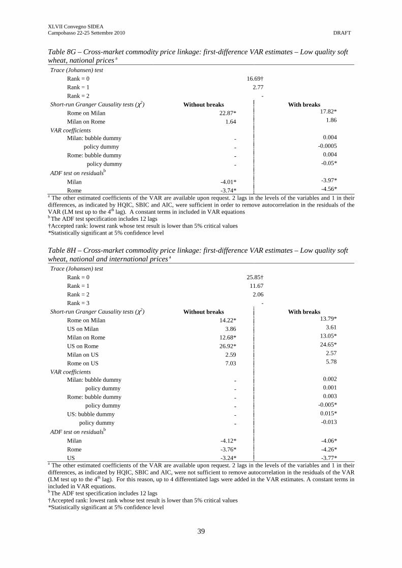
XLVII Convegno SIDEA Campobasso 22-25 Settembre 2010 DRAFT
39
Table 8G – Cross-market commodity price linkage: first-difference VAR estimates – Low quality soft wheat, national prices a Trace (Johansen) test
Rank = 0 16.69†
Rank = 1 2.77
Rank = 2 -
Short-run Granger Causality tests (χ2) Without breaks With breaks Rome on Milan 22.87* 17.82*
Milan on Rome 1.64 1.86
VAR coefficients
Milan: bubble dummy - 0.004
policy dummy - -0.0005
Rome: bubble dummy - 0.004
policy dummy - -0.05*
ADF test on residualsb
Milan -4.01* -3.97*
Rome -3.74* -4.56* a The other estimated coefficients of the VAR are available upon request. 2 lags in the levels of the variables and 1 in their differences, as indicated by HQIC, SBIC and AIC, were sufficient in order to remove autocorrelation in the residuals of the VAR (LM test up to the 4th lag). A constant terms in included in VAR equations b The ADF test specification includes 12 lags †Accepted rank: lowest rank whose test result is lower than 5% critical values *Statistically significant at 5% confidence level Table 8H – Cross-market commodity price linkage: first-difference VAR estimates – Low quality soft wheat, national and international prices a
Trace (Johansen) test
Rank = 0 25.85†
Rank = 1 11.67
Rank = 2 2.06
Rank = 3 -
Short-run Granger Causality tests (χ2) Without breaks With breaks Rome on Milan 14.22* 13.79*
US on Milan 3.86 3.61
Milan on Rome 12.68* 13.05*
US on Rome 26.92* 24.65*
Milan on US 2.59 2.57
Rome on US 7.03 5.78
VAR coefficients
Milan: bubble dummy - 0.002
policy dummy - 0.001
Rome: bubble dummy - 0.003
policy dummy - -0.005*
US: bubble dummy - 0.015*
policy dummy - -0.013
ADF test on residualsb
Milan -4.12* -4.06*
Rome -3.76* -4.26*
US -3.24* -3.77* a The other estimated coefficients of the VAR are available upon request. 2 lags in the levels of the variables and 1 in their differences, as indicated by HQIC, SBIC and AIC, were not sufficient to remove autocorrelation in the residuals of the VAR (LM test up to the 4th lag). For this reason, up to 4 differentiated lags were added in the VAR estimates. A constant terms in included in VAR equations. b The ADF test specification includes 12 lags †Accepted rank: lowest rank whose test result is lower than 5% critical values *Statistically significant at 5% confidence level
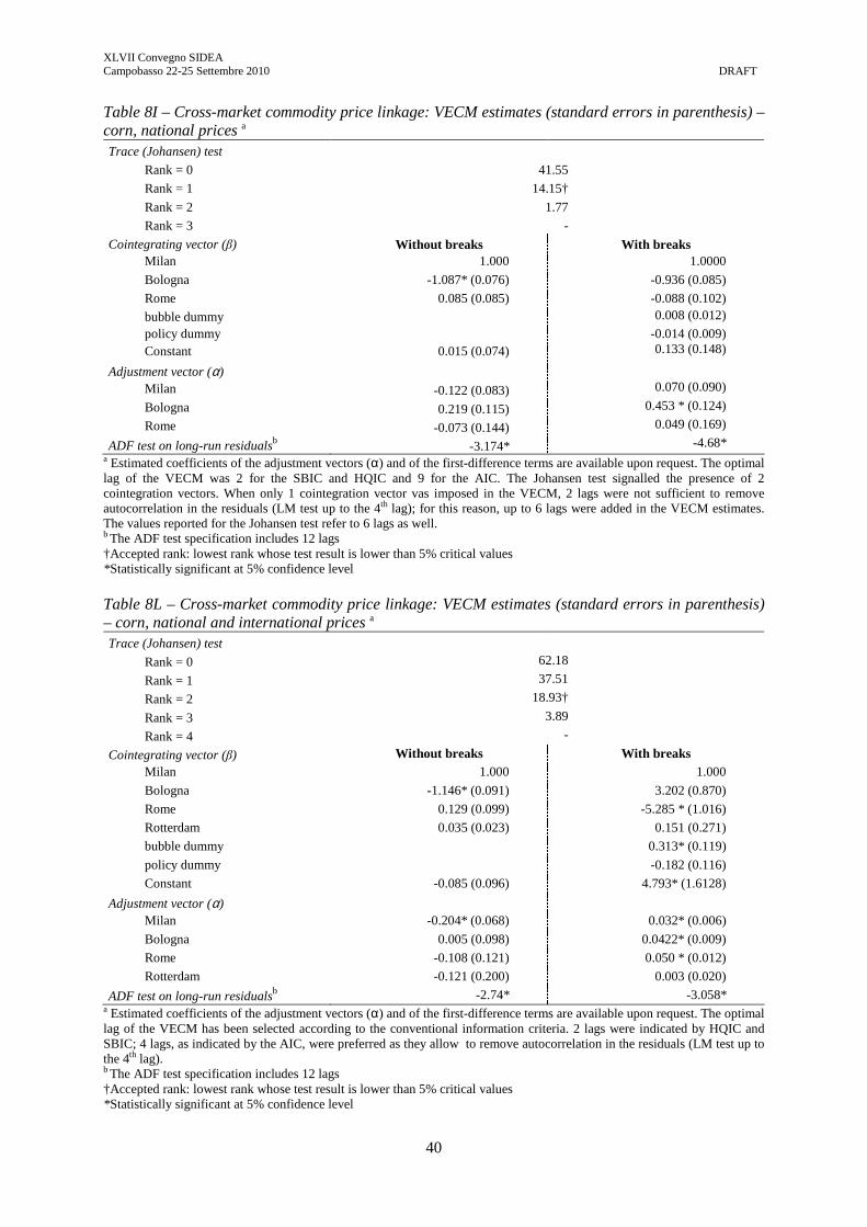
XLVII Convegno SIDEA Campobasso 22-25 Settembre 2010 DRAFT
40
Table 8I – Cross-market commodity price linkage: VECM estimates (standard errors in parenthesis) – corn, national prices a Trace (Johansen) test
Rank = 0 41.55
Rank = 1 14.15†
Rank = 2 1.77
Rank = 3 -
Cointegrating vector (β) Without breaks With breaks Milan 1.000 1.0000
Bologna -1.087* (0.076) -0.936 (0.085)
Rome 0.085 (0.085) -0.088 (0.102)
bubble dummy 0.008 (0.012)
policy dummy -0.014 (0.009) Constant 0.015 (0.074) 0.133 (0.148)
Adjustment vector (α) Milan -0.122 (0.083) 0.070 (0.090)
Bologna 0.219 (0.115) 0.453 * (0.124)
Rome -0.073 (0.144) 0.049 (0.169)
ADF test on long-run residualsb -3.174* -4.68* a Estimated coefficients of the adjustment vectors (α) and of the first-difference terms are available upon request. The optimal lag of the VECM was 2 for the SBIC and HQIC and 9 for the AIC. The Johansen test signalled the presence of 2 cointegration vectors. When only 1 cointegration vector vas imposed in the VECM, 2 lags were not sufficient to remove autocorrelation in the residuals (LM test up to the 4th lag); for this reason, up to 6 lags were added in the VECM estimates. The values reported for the Johansen test refer to 6 lags as well. b The ADF test specification includes 12 lags †Accepted rank: lowest rank whose test result is lower than 5% critical values *Statistically significant at 5% confidence level Table 8L – Cross-market commodity price linkage: VECM estimates (standard errors in parenthesis) – corn, national and international prices a Trace (Johansen) test
Rank = 0 62.18
Rank = 1 37.51
Rank = 2 18.93†
Rank = 3 3.89
Rank = 4 -
Cointegrating vector (β) Without breaks With breaks
Milan 1.000 1.000
Bologna -1.146* (0.091) 3.202 (0.870)
Rome 0.129 (0.099) -5.285 * (1.016)
Rotterdam 0.035 (0.023) 0.151 (0.271)
bubble dummy 0.313* (0.119)
policy dummy -0.182 (0.116)
Constant -0.085 (0.096) 4.793* (1.6128)
Adjustment vector (α)
Milan -0.204* (0.068) 0.032* (0.006)
Bologna 0.005 (0.098) 0.0422* (0.009)
Rome -0.108 (0.121) 0.050 * (0.012)
Rotterdam -0.121 (0.200) 0.003 (0.020)
ADF test on long-run residualsb -2.74* -3.058* a Estimated coefficients of the adjustment vectors (α) and of the first-difference terms are available upon request. The optimal lag of the VECM has been selected according to the conventional information criteria. 2 lags were indicated by HQIC and SBIC; 4 lags, as indicated by the AIC, were preferred as they allow to remove autocorrelation in the residuals (LM test up to the 4th lag). b The ADF test specification includes 12 lags †Accepted rank: lowest rank whose test result is lower than 5% critical values *Statistically significant at 5% confidence level

XLVII Convegno SIDEA Campobasso 22-25 Settembre 2010 DRAFT
41
Table 8M – Cross-market commodity price linkage: first-difference VAR estimates – barley, national prices a Trace (Johansen) test
Rank = 0 17.15†
Rank = 1 5.31
Rank = 2 -
Short-run Granger Causality tests (χ2) Without breaks With breaks Foggia on Bologna 15.60* 15.60*
Bologna on Foggia 34.37* 30.25*
VAR coefficients
Bologna: bubble dummy - 0.004
policy dummy - -0.011*
Foggia: bubble dummy - 0.002
policy dummy - -0.002
ADF test on residualsb
Bologna -3.38* -3.91*
Foggia -3.74* -3.76* a The other estimated coefficients of the VAR are available upon request. The optimal lag of the VECM has been selected according to the conventional information criteria. 2 lags in the levels of the variables and 1 in their differences were indicated by HQIC and SBIC; 9 lags in the levels and 8 in the differences, as indicated by the AIC, were preferred as they allow to remove autocorrelation in the residuals (LM test up to the 4th lag). A constant terms in included in VAR equations b The ADF test specification includes 12 lags †Accepted rank: lowest rank whose test result is lower than 5% critical values *Statistically significant at 5% confidence level Table 8N – Cross-market commodity price linkage: first-difference VAR estimates – barley, national and international prices a Trace (Johansen) test
Rank = 0 29.18†
Rank = 1 12.40
Rank = 2 2.54
Rank = 3 -
Short-run Granger Causality tests (χ2) Without breaks With breaks Foggia on Bologna 7.64 7.37
US on Bologna 1.94 2.25
Bologna on Foggia 10.18* 6.89
US on Foggia 2.99 3.05
Bologna on US 5.40 3.21
Foggia on US 4.21 4.56
VAR coefficients
Bologna: bubble dummy - 0.004
policy dummy - -0.009*
Foggia: bubble dummy - 0.002
policy dummy - -0.001
US: bubble dummy - -0.003
policy dummy - -0.007
ADF test on residualsb
Bologna -3.72* -4.74*
Foggia -3.81* -3.89*
US -3.91* -3.84* a The other estimated coefficients of the VAR are available upon request. 2 lags in the levels of the variables and 1 in their differences, as indicated by HQIC, SBIC and AIC, were not sufficient to remove autocorrelation in the residuals of the VAR (LM test up to the 4th lag). For this reason, up to 3 differentiated lags were added in the VAR estimates. A constant terms in included in VAR equations b The ADF test specification includes 12 lags †Accepted rank: lowest rank whose test result is lower than 5% critical values *Statistically significant at 5% confidence level

XLVII Convegno SIDEA Campobasso 22-25 Settembre 2010 DRAFT
42
Table 9A – Cross-commodity market price linkage: first-difference VAR estimates – Northern Italy (Milan) a,c Trace (Johansen) test
Rank = 0 29.54† Rank = 1 13.17 Rank = 2 2.62 Rank = 3 -
Short-run Granger Causality tests (χ2) Without breaks With breaks Soft Wheat (high quality) on Soft Wheat 27.07* 24.94* Soft Wheat (high quality) on Corn 7.68* 4.32 Soft Wheat on Soft Wheat (high quality) 6.32* 4.75 Soft Wheat on Corn 0.88 1.19 Corn on Soft Wheat (high quality) 0.54 0.23 Corn on Soft Wheat 1.69 1.47
VAR coefficients Soft Wheat (high quality): bubble dummy - 0.009*
policy dummy - -0.013* Soft Wheat: bubble dummy - 0.001
policy dummy - 0.004 Corn: bubble dummy - 0.004
policy dummy - -0.009* ADF test on residualsb
Soft Wheat (high quality) -3,87* -4.67* Soft Wheat -3.50* -3.71* Corn -4.04* -4.66*
a The other estimated coefficients of the VAR are available upon request. The optimal lag (s=2) has been selected according to the conventional information criteria. . A constant terms in included in VAR equations b The ADF test specification includes 12 lags c Only in this table “Soft Wheat” indicates low and medium quality †Accepted rank: lowest rank whose test result is lower than 5% critical values *Statistically significant at 5% confidence level
Table 9B – Cross-commodity market price linkage: VECM estimates (standard errors in parenthesis) – Central-Northern Italy (Bologna) a Trace (Johansen) test
Rank = 0 59.55 Rank = 1 24.62† Rank = 2 12.14 Rank = 3 3.88 Rank = 4 -
Cointegrating vector (β) Without breaks With breaks Soft Wheat 1.000 1.000 Durum Wheat -0.145* (0.058) -0.406 (0.252) Corn 0.876* (0.162) 2.706* (0.577) Barley -1.401* (0.161) -2.974* (0.568) bubble dummy - 0.238 (0.194) policy dummy - 0.312 (0.151) Constant -1.721* (0.316) -1.729 (1.537)
Adjustment vector (α) Soft Wheat -0.032 (0.019) -0.001 (0.006) Durum Wheat 0.019 (0.026) 0.001 (0.008) Corn -0.127* (0.024) -0.040* (0.008) Barley -0.012 (0.018) -0.007 (0.005)
ADF test on long-run residualsb -3.86* -3.25* a Estimated coefficients of the first-difference terms are available upon request. The optimal lag (s=5) of the VECM has been selected according to the conventional information criteria b The ADF test specification includes 12 lags †Accepted rank: lowest rank whose test result is lower than 5% critical values *Statistically significant at 5% confidence level

XLVII Convegno SIDEA Campobasso 22-25 Settembre 2010 DRAFT
43
Table 9C – Cross-commodity market price linkage: first-difference VAR estimates – Central-Southern Italy (Rome) a Trace (Johansen) test
Rank = 0 28.79† Rank = 1 15.72 Rank = 2 4.21 Rank = 3 -
Short-run Granger Causality tests (χ2) Without breaks With breaks Durum Wheat on Soft Wheat 0.187 0.720 Durum Wheat on Corn 0.392 0.475 Soft Wheat on Durum Wheat 21.81* 18.732* Soft Wheat on Corn 15.24* 13.586* Corn on Durum Wheat 0.480 0.486 Corn on Soft Wheat 2.970 2.704
VAR coefficients Durum Wheat: bubble dummy - 0.012*
policy dummy - -0.007* Soft Wheat: bubble dummy - 0.003*
policy dummy - -0.006* Corn: bubble dummy - 0.004
policy dummy - -0.009 ADF test on residualsb
Durum Wheat -3.123* -4.06* Soft Wheat -3.773* -4.26* Corn -4.069* -4.27*
a The other estimated coefficients of the VAR are available upon request. The optimal lag (s=3) has been selected according to the conventional information criteria. A constant terms in included in VAR equations b The ADF test specification includes 12 lags †Accepted rank: lowest rank whose test result is lower than 5% critical values *Statistically significant at 5% confidence level
Table 9D – Cross-commodity market price linkage: VECM estimates (standard errors in parenthesis) – International (Rotterdam) a Trace (Johansen) test
Rank = 0 73.73 Rank = 1 34.66† Rank = 2 10.55 Rank = 3 2.54
Cointegrating vector (β) Without breaks With breaks Soft Wheat 1.000 1.000 Durum Wheat -0.597* (0.065) -0.588 (0.271) Corn -0.414* (0.145) 4.037* (0.795) Barley 0.460* (0.130) -3.836* (0.660) bubble dummy - 0,799 (0,242) policy dummy - -0,347 (0,198) Constant -2.283* (0.405) -2.440 (1.804)
Adjustment vector (α) Soft Wheat -0.052 (0.034) 0.001 (0.016) Durum Wheat 0.189* (0.033) 0.028* (0.015) Corn 0.011 (0.036) -0.025 (0.016) Barley 0.042 (0.032) 0.039* (0.014)
ADF test on long-run residualsb -3,86* -3,39* a Estimated coefficients of the first-difference terms are available upon request. The optimal lag (s=3) of the VECM has been selected according to the conventional information criteria b The ADF test specification includes 12 lags †Accepted rank: lowest rank whose test result is lower than 5% critical values *Statistically significant at 5% confidence level

XLVII Convegno SIDEA Campobasso 22-25 Settembre 2010 DRAFT
44
Figure 1 – The price bubble: cereal price series over the four years between April 2006 and April 2010 (see Appendix for price codes)
0,0
100,0
200,0
300,0
400,0
500,0
600,0
700,0
800,0
ap
r-0
6
lug
-06
ott
-06
ge
n-0
7
ap
r-0
7
lug
-07
ott
-07
ge
n-0
8
ap
r-0
8
lug
-08
ott
-08
ge
n-0
9
ap
r-0
9
lug
-09
ott
-09
ge
n-1
0
ap
r-1
0
fd_bm_ca
fd_bm_fo
fd_bm_na
fd_fi_bo
fd_fi_ca
fd_fi_fo
fd_fi_rofd_me_fo
ft_bm_mi
ft_bm_ro
ft_fi_bo
ft_fi_mi
ft_gf_bo
ft_vs_bo
ft_vs_mi
mais_bo
mais_mi
mais_na
mais_ro
or_bo
or_focwrs_can
dns_us
hrw_us
srw_us
cwad_can
mais_us
or_us
€/ton

XLVII Convegno SIDEA Campobasso 22-25 Settembre 2010 DRAFT
45
Figure 2 – Seasonality: weekly averages of prices over the whole period and the ascending and descending part of the bubble (see Appendix for price codes)
Weekly averages: April 2006 - April 2010
0
50
100
150
200
250
300
350
400
1 2 3 4 5 6 7 8 9 10 11 12 13 14 15 16 17 18 19 20 21 22 23 24 25 26 27 28 29 3031 32 33 34 35 36 37 38 39 40 41 42 43 44 45 46 47 48 49 50 51 52
fd_bm_fofd_bm_nafd_fi_bofd_fi_cafd_fi_fofd_fi_rofd_me_foft_bm_mift_bm_roft_fi_boft_fi_mift_gf_boft_vs_boft_vs_mimais_bomais_mimais_namais_roor_boor_focwrs_candns_ushrw_ussrw_uscwad_canmais_usor_us
€/ton
Weekly averages: April 2008 - April 2010
0
50
100
150
200
250
300
350
400
450
1 2 3 4 5 6 7 8 9 10 11 12 13 14 15 16 17 18 19 20 21 22 23 24 25 26 27 28 29 3031 32 33 34 35 36 37 38 39 40 41 42 43 44 45 46 47 48 49 50 51 52
fd_bm_fofd_bm_nafd_fi_bofd_fi_cafd_fi_fofd_fi_rofd_me_foft_bm_mift_bm_roft_fi_boft_fi_mift_gf_boft_vs_boft_vs_mimais_bomais_mimais_namais_roor_boor_focwrs_candns_ushrw_ussrw_uscwad_canmais_usor_us
€/ton
Weekly averages: April 2006 - April 2008
0
50
100
150
200
250
300
350
400
450
500
1 2 3 4 5 6 7 8 9 10 11 12 13 14 15 16 17 18 19 20 21 22 23 24 25 26 27 28 29 3031 32 33 34 35 36 37 38 39 40 41 42 43 44 45 46 47 48 49 50 51 52
fd_bm_cafd_bm_fofd_bm_nafd_fi_bofd_fi_cafd_fi_fofd_fi_rofd_me_foft_bm_mift_bm_roft_fi_boft_fi_mift_gf_boft_vs_boft_vs_mimais_bomais_mimais_namais_roor_boor_focwrs_candns_ushrw_ussrw_uscwad_canmais_usor_us
€/ton
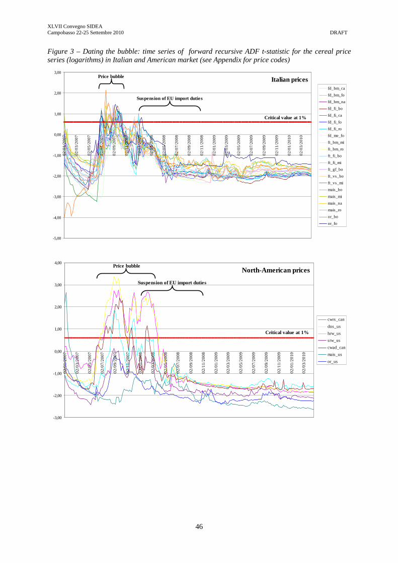
XLVII Convegno SIDEA Campobasso 22-25 Settembre 2010 DRAFT
46
Figure 3 – Dating the bubble: time series of forward recursive ADF t-statistic for the cereal price series (logarithms) in Italian and American market (see Appendix for price codes)
-5,00
-4,00
-3,00
-2,00
-1,00
0,00
1,00
2,00
3,00
02
/01
/20
07
02
/03
/20
07
02
/05
/20
07
02
/07
/20
07
02
/09
/20
07
02
/11
/20
07
02
/01
/20
08
02
/03
/20
08
02
/05
/20
08
02
/07
/20
08
02
/09
/20
08
02
/11
/20
08
02
/01
/20
09
02
/03
/20
09
02
/05
/20
09
02
/07
/20
09
02
/09
/20
09
02
/11
/20
09
02
/01
/20
10
02
/03
/20
10
fd_bm_ca
fd_bm_fo
fd_bm_na
fd_fi_bo
fd_fi_ca
fd_fi_fo
fd_fi_ro
fd_me_fo
ft_bm_mi
ft_bm_ro
ft_fi_bo
ft_fi_mi
ft_gf_bo
ft_vs_bo
ft_vs_mi
mais_bo
mais_mi
mais_na
mais_ro
or_bo
or_fo
Suspension of EU import duties
Price bubble
Critical value at 1%
Italian prices
-3,00
-2,00
-1,00
0,00
1,00
2,00
3,00
4,00
02
/01
/20
07
02
/03
/20
07
02
/05
/20
07
02
/07
/20
07
02
/09
/20
07
02
/11
/20
07
02
/01
/20
08
02
/03
/20
08
02
/05
/20
08
02
/07
/20
08
02
/09
/20
08
02
/11
/20
08
02
/01
/20
09
02
/03
/20
09
02
/05
/20
09
02
/07
/20
09
02
/09
/20
09
02
/11
/20
09
02
/01
/20
10
02
/03
/20
10
cwrs_can
dns_us
hrw_us
srw_us
cwad_can
mais_us
or_us
Critical value at 1%
North-American pricesPrice bubble
Suspension of EU import duties

XLVII Convegno SIDEA Campobasso 22-25 Settembre 2010 DRAFT
47
Figure 4 – Impulse Response Functions of the endogenous prices (Rome and Foggia) in Durum Wheat markets (ordering: Bologna, Rome, Foggia, Rotterdam; model with bubble and policy dummies)
-2,0
-1,0
0,0
1,0
2,0
3,0
4,0
0 1 2 3 4 5 6 7 8 9 10 11 12
Bologna on Roma Foggia on Roma Rotterdam on Roma
Bologna on Foggia Roma on Foggia Rotterdam on Foggia
Figure 5 – Significant (according to Granger Causality tests) Impulse Response Functions in Soft Wheat (high quality) markets (ordering: Bologna, Milan, Rotterdam; model with bubble and policy dummies)
0
0,1
0,2
0,3
0,4
0,5
0 1 2 3 4 5 6 7 8 9 10 11 12
Bologna on Milano Rotterdam on Milano Rotterdam on Bologna

XLVII Convegno SIDEA Campobasso 22-25 Settembre 2010 DRAFT
48
Figure 6 – Significant (according to Granger Causality tests) Impulse Response Functions in Soft Wheat (medium quality) markets (ordering: Bologna, Milan, Rotterdam; model with bubble and policy dummies)
0
0,1
0,2
0,3
0,4
0,5
0,6
0,7
0 1 2 3 4 5 6 7 8 9 10 11 12
Bologna on Milano Bologna on Rotterdam Rotterdam on Bologna
Figure 7 – Significant (according to Granger Causality tests) Impulse Response Functions in Soft Wheat (low quality) markets (ordering: Milan, Rome, Rotterdam; model with bubble and policy dummies)
-0,1
0
0,1
0,2
0,3
0,4
0,5
0,6
0,7
0 1 2 3 4 5 6 7 8 9 10 11 12
Roma on Milano Milano on Roma Rotterdam on Roma

XLVII Convegno SIDEA Campobasso 22-25 Settembre 2010 DRAFT
49
Figure 8 – Impulse Response Functions of the endogenous price (Milan) in Corn markets (ordering: Milan, Bologna, Rome, Rotterdam; model witht bubble and policy dummies)
-0,04
-0,03
-0,02
-0,01
0
0,01
0,02
0,03
0 1 2 3 4 5 6 7 8 9 10 11 12
Milano on Bologna Milano on Roma Bologna on Milano
Bologna on Roma Roma on Milano Roma on Bologna
Rotterdam on Milano Rotterdam on Bologna Rotterdam on Roma
Figure 9 – Significant (according to Granger Causality tests) Impulse Response Functions in Barley markets (ordering: Bologna, Foggia; model with bubble and policy dummies, only national prices)
-0,2
-0,1
0
0,1
0,2
0,3
0,4
0 1 2 3 4 5 6 7 8 9 10 11 12
Bologna on Foggia Foggia on Bologna

XLVII Convegno SIDEA Campobasso 22-25 Settembre 2010 DRAFT
50
Figure 10 – Significant (according to Granger Causality tests) Impulse Response Functions in Milan and Rome markets (ordering: Soft Wheat, Durum Wheat, Corn, Barley; model with bubble and policy dummies)
-0,2
0
0,2
0,4
0,6
0,8
0 1 2 3 4 5 6 7 8 9 10 11 12
Milano: Soft Wheat (high quality) on Soft Wheat (low and medium quality)
Roma: Soft Wheat on Durum Wheat
Roma: Soft Wheat on Corn
Figure 11– Impulse Response Functions of the endogenous price (Corn) in Bologna markets (ordering: Softt Wheat, Durum Wheat, Corn, Barley; model with bubble and policy dummies)
-0,5
0
0,5
1
1,5
2
2,5
0 1 2 3 4 5 6 7 8 9 10 11 12
Soft Wheat on Corn Durum Wheat on Corn Barley on Corn

XLVII Convegno SIDEA Campobasso 22-25 Settembre 2010 DRAFT
51
Figure 12 – Impulse Response Functions of the endogenous price (Durum Wheat) in Rotterdam markets (ordering: Soft Wheat, Durum Wheat, Corn, Barley; model with bubble and policy dummies)
-1,5
-1,0
-0,5
0,0
0,5
1,0
1,5
2,0
0 1 2 3 4 5 6 7 8 9 10 11 12
Soft Wheat on Durum Wheat Corn on Durum Wheat Barley on Durum Wheat

XLVII Convegno SIDEA Campobasso 22-25 Settembre 2010 DRAFT
52
APPENDIX
Table A.1 – Codification and description of the prices adopted in the analysis
Price Code Product Description Market Place fd_bm_ca Durum Wheat, Buono Mercantile Catania
fd_bm_fo Durum Wheat, Buono Mercantile Foggia
fd_bm_na Durum Wheat, Buono Mercantile Naples
fd_fi_bo Durum Wheat, Fino Bologna
fd_fi_ca Durum Wheat, Fino Catania
fd_fi_fo Durum Wheat, Fino Foggia
fd_fi_ro Durum Wheat, Fino Rome
fd_me_fo Durum Wheat, Mercantile Foggia
ft_bm_mi Soft Wheat, Buono Mercantile Milan
ft_bm_ro Soft Wheat, Buono Mercantile Rome
ft_fi_bo Soft Wheat, Fino Bologna
ft_fi_mi Soft Wheat, Fino Milan
ft_gf_bo Soft Wheat, Grani di Forza Bologna
ft_vs_bo Soft Wheat, Varietà Speciali Bologna
ft_vs_mi Soft Wheat, Varietà Speciali Milan
mais_bo Maize, Ibrido Nazionale Bologna
mais_mi Maize, Ibrido Nazionale Milan
mais_na Maize, Ibrido Nazionale Naples
mais_ro Maize, Ibrido Nazionale Rome
or_bo Barley, Nazionale Bologna
or_fo Barley, Nazionale Foggia
cwrs_cana Wheat, Canada Western Red Spring (CWRS) Canada, St Lawrence
dns_usa Wheat, Dark Northern Spring (DNS) US, Gulf
hrw_usa Wheat, Hard Red Winter (HRW) US, Gulf
srw_usa Wheat, Soft Red Winter (HRW) US, Gulf
cwad_cana Wheat, Canada Western Amber Durum (CWAD) Canada, St Lawrence
mais_usa Maize, #3 Yellow Corn (3YC) US, Gulf
or_usa Barley, Pacific NorthWestern (PNW) US, West a CIF price - Rotterdam

XLVII Convegno SIDEA Campobasso 22-25 Settembre 2010 DRAFT
53
Table A.2 – Price groups for the analysis of price linkages (VECM of first-difference VAR models)
Group of Interdependent Commodities/Markets Property of the Series Estimated Model Fixed Commodity-Cross Space
DURUM WHEAT VECM
fd_fi_bo I(1)
fd_fi_ro I(1)
fd_fi_fo I(1)
cwrs_cana I(1) + explosive root
SOFT WHEAT (High Quality) First-difference VAR
ft_vs_mi I(1)
ft_vs_bo I(1)
hrw_usa I(1)
SOFT WHEAT (Medium Quality) First-difference VAR
ft_fi_mi I(1)
ft_fi_bo I(1)
hrw_usa I(1)
SOFT WHEAT (Low Quality) First-difference VAR
ft_bm_mi I(1)
ft_bm_ro I(1)
hrw_usa I(1)
CORN VECM
mais_mi I(1)
mais_bo I(1)
mais_ro I(1)
mais_usa I(1)
BARLEY First-difference VAR
or_bo I(1) + explosive root
or_ro I(1)
ors_usa I(1)
Fixed Space-Cross Commodity NORTHERN ITALY (Milan) First-difference VAR
ft_vs_mi I(1)
ft_fi_mi I(1)
mais_mi I(1)
CENTRAL-NORTHERN ITALY (Bologna) VECM
ft_fi_bo I(1)
fd_fi_bo I(1)
mais_bo I(1)
or_bo I(1) + explosive root
CENTRAL-SOUTHERN ITALY (Rome) First-difference VAR
ft_bm_ro I(1)
fd_fi_ro I(1)
mais_ro I(1)
INTERNATIONAL (Rotterdam) VECM
hrw_usa I(1)
cwad_cana I(1) + explosive root
mais_usa I(1)
or_usa I(1) a CIF price - Rotterdam