Agricultural diversification and specialisation: the...
147
Agricultural diversification and specialisation: the impact on smallholders’ farm efficiency in China By LIHUA LI THESIS Submitted in partial fulfilment of the requirements for the degree of DOCTOR OF PHILOSOPHY School of Science and Health Western Sydney University Penrith, NSW, 2751
Transcript of Agricultural diversification and specialisation: the...
Agricultural diversification and specialisation: the impact on
smallholders’ farm efficiency in China
By
LIHUA LI
THESIS
Submitted in partial fulfilment of the requirements for the degree of
DOCTOR OF PHILOSOPHY
School of Science and Health
Western Sydney University
Penrith, NSW, 2751
i
Statement of authentication
Author: Lihua Li
Degree: Doctor of Philosophy
Date: 31st January 2016
I certify that the work presented in this thesis in fulfilment of the requirement for the
degree of Doctor of Philosophy is, to the best of my knowledge, original, except for those
parts as acknowledged in the text by reference, and that the material has not been
submitted, either in full or in part, for any degree enrolled at this or any other institution.
I certify that I have complied in all other respects with the rules, requirements, procedures
and policy relating to the award of this degree at the Western Sydney University.
Lihua Li
ii
Acknowledgements
I wish to express my gratitude to the ACIAR John Allwright Fellowship (Australian
Centre of International Agricultural Research) for sponsoring my study at Western
Sydney University.
I thank my principal supervisor, Professor Bill Bellotti, for nominating me for the
fellowship, and I am especially grateful for his generous help, encouragement and
understanding throughout my study. Sincere thanks also to my co-supervisors Dr Adam
Komarek, Dr Sriram Shankar, and Dr Maria Estela Varua, for their guidance and shared
knowledge relating to farming systems, efficiency analysis and econometrics of this
thesis. Copyediting of the thesis was performed by Jera Editing Services.

iii
Table of Contents
Chapter 1 Introduction ................................................................................................ 1
1.1 Structural change and the notion of agriculture for development ................................... 1
1.2 The role of agriculture in China’s transformation ............................................................. 3
1.3 Problems and the research rationale ................................................................................ 4
1.4 Hypotheses and objectives ................................................................................................ 5
1.5 Methodology and data ...................................................................................................... 8
1.7 Thesis organisation .......................................................................................................... 11
Chapter 2 Agricultural diversification and regional development in China ................. 13
2.1 Agricultural diversification in relation to regional variations—the hypothesis .............. 13
2.2 Structural change and agricultural diversification – the conceptual framework ............ 15
2.2.3 The challenges of structural change and agricultural diversification ................... 20
2.3 Structural change and agricultural transformation in China – an overview ................... 22
2.3.1 Distinctive economic features, consistent transformation patterns ................... 22
2.3.2 Transformation in agriculture, stages and policies .............................................. 28
2.4. Quantifying agricultural diversification in China ............................................................ 30
2.4.1 Methods ............................................................................................................... 30
2.4.2 Data ...................................................................................................................... 31
2.5 Results ............................................................................................................................. 32
2.5.1 Agricultural diversification in relation to growth – regional comparison ............ 32
2.5.2 Agricultural transformation and its interdependence with non-agricultural sector
in underdeveloped regions – the case of Gansu province ............................................ 34
Chapter 3 The farm level production specialisation and commercialisation ................ 39
3.1 Introduction ..................................................................................................................... 39
3.2 Theoretical foundations .................................................................................................. 40
3.3 The trend of the farm level specialisation ....................................................................... 42
iv
3.3.1 Measuring smallholders’ production specialisation ............................................. 42
3.3.2 Study area ............................................................................................................. 42
3.3.3 Household survey ................................................................................................. 44
3.4 Farm specialisation and commercialisation .................................................................... 49
3.4.1 Definition and measure of commercialisation ..................................................... 49
3.4.2 The econometric model ....................................................................................... 50
3.4.3 Specification and variables affecting commercialisation ..................................... 50
3.4.5 Estimation of the Simultaneous-Equations Model ............................................... 53
3.5 Results and discussion ..................................................................................................... 56
Chapter 4 The impact of farm specialisation on efficienc ........................................... 67
4.1 Introduction ..................................................................................................................... 67
4.2 Conceptual framework .................................................................................................... 71
4.2.1 Trade-off between diversification and specialisation .......................................... 71
4.2.2 Specialisation, efficiency, and economies of scale – definitions and correlations72
4.3 Studies of Farm Efficiency ............................................................................................... 73
4.3.1 Are larger farms more efficient? -- The relationship between farm size and
efficiency in developed countries .................................................................................. 74
4.3.2 Small but efficient – subsistence farms in developing countries ......................... 75
4.3.3 Previous efficiency studies of China ..................................................................... 76
4.4 Methods .......................................................................................................................... 78
4.4.1 Production efficiency: concept and measurement .............................................. 78
4.4.2 Impacts of specialisation on efficiency ................................................................. 87
4.5 Results and Discussion ..................................................................................................... 89
4.5.1 Efficiency estimates .............................................................................................. 89
4.5.2 Factors explaining efficiencies .............................................................................. 93
Chapter 5 Conclusion and policy implication............................................................ 101
v
5.1 Conclusion ..................................................................................................................... 101
5.1.1 China’s structural change and agricultural diversification ................................. 101
5.1.2 Smallholder specialisation and commercialisation: an interplay ....................... 102
5.1.3 Specialisation of small farms: the gain in production efficiency ........................ 103
5.2 Policy implications ......................................................................................................... 104
5.3 Limitations of the study ................................................................................................. 106
References .............................................................................................................. 108
Appendix ................................................................................................................ 122

vi
List of Tables
Table 3.1 Farm income composition and growth of selected commodities in Qingyang,
1995–2010 ························································································································ 43
Table 3.2 Environmental and geographical data for the three study areas ····················· 44
Table 3.3 Durbin-Wu-Hausman simultaneity test ···························································· 47
Table 3.4 Relationship between crop commercialisation and crop specialisation ·········· 61
Table 3.5 Relationship between Farm commercialisation and Farm specialisation ········ 62
Table 3.6 Relationship between livestock commercialisation and livestock specialisation
··········································································································································· 63
Table 3.7 Regression on crop specialisation ………………………………………………………………..65
Table 3.8 Robustness Check of the effect of Asset Vs Total Income/Income per capita
··········································································································································· 66
Table 4.1 Summary statistics of inputs outputs ······························································· 86
Table 4.2 Summary Statistics and Frequency Distribution of Efficiency Measures ········· 89
Table 4.3 Radial and slack analysis of inputs ···································································· 90
Table 4.4 Share of farms operating under CRS, IRS, and DRS ·········································· 92
vii
List of Figures
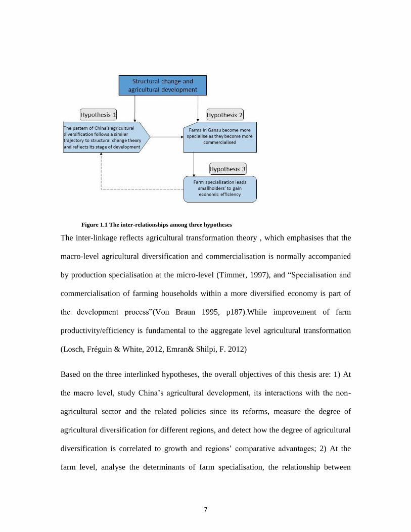
Figure 1.1 The inter-relationships among three hypotheses ··········································· 7
Figure 2.1 The Relationship between Diversification and Agricultural Transformation ·· 20
Figure 2.2 Comparison of structural change and growth among China and selected
countries ··························································································································· 25
Figure 2.3 Diversification level and GDP per capita for national average and six regions,
1978-2012 ························································································································· 32
Figure 2.4 Sectoral shares in GDP and employment, Gansu province and national
average ······························································································································ 36
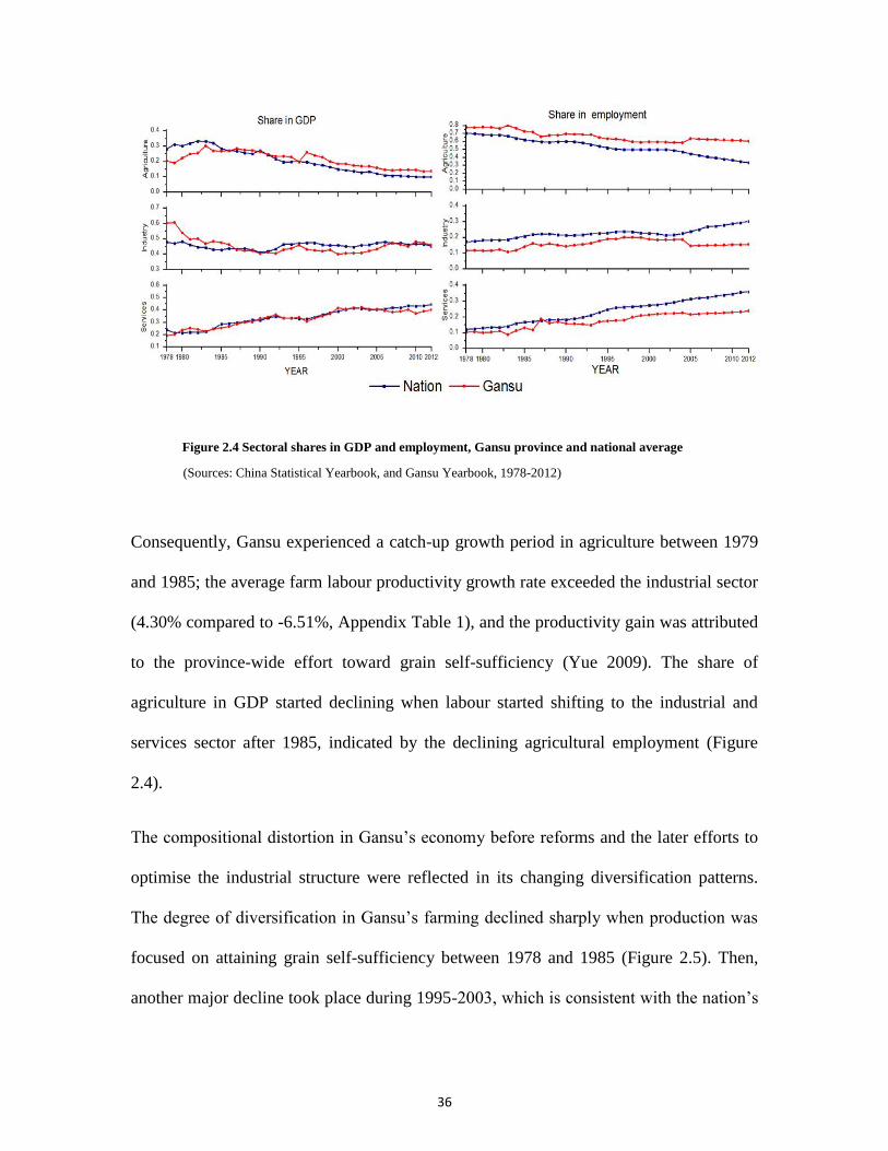
Figure 2.5 Changing of agricultural diversification, China and Gansu province ··············· 36
Figure 3.1 Locations of the Three Case Study Areas ························································ 46
Figure 3.2 Specialisation versus income per capita for surveyed farms in Qingyang ······ 47
Figure 3.3 Distribution of specialisation cross three locations ········································· 48
Figure 4.1 Input-Oriented Measure for Technical, Allocative and Cost Efficiency ··········· 80
Figure 4.2 Constant, Increasing and Decreasing Returns to Scale ··································· 83
viii
Abstract
Structural change is a major engine in fostering a country’s growth. In the agricultural
sector, diversification is the commonly used development strategy to increase the rural
sector’s flexibility, to respond to improving technologies and market conditions. From an
agricultural transformation perspective, this thesis consists of three interrelated studies.
The first study examines agricultural development and transformation during China’s
socio-economic reforms. In particular, it empirically tests the question of whether
economic development results in agricultural diversification at the national and regional
level in the Chinese context, given its fast growth and special paths of transition and
development. The degree of agricultural diversification was quantitatively measured at a
regional scale using the Herfindahl index. An underdeveloped region, Gansu province in
Northwest China, was studied to provide insights into the interaction among structural
change, agricultural diversification, and implemented development policies. Aggregate-
level analyses suggest that, although economic growth in China is unique, its pattern of
agricultural transformation is consistent with those of other developing countries. China’s
agricultural sector became more diversified as the economy grew. Agricultural
diversification appears to relate to a region’s comparative advantage and the relative
importance of agriculture in the region.
The second study explores the interrelationship between smallholders’ production
specialisation and commercialisation.This study first ascertains whether China’s macro-
level agricultural diversification is accompanied by farm specialisation. It then explores
earlier studies,that were at a more conceptual level, that propose a relationship between
ix
commericalisation and specialisation by providing modest insights into farm-level
commericalisation and specialisation.Using a set of simultaneousequations,a two-way
interrelationship between specialisation and commercialisation were confirmed,
suggesting that farmers’ decisions on farm commercialisation and production
specialisation are actually separate and interacting. The results further suggest that higher
asset endowments indeed enable small farmers to specialise in production where they
have a comparative advantage, while assets, especially capital, actually reduce farmers’
incentives to sell their surplus to get cash.
The third study examines the impact of specialisation on farm efficiencies. Farms’
technical, allocative, and scale efficiencies were measured by non-parametric frontier
analysis. Then the impact of specialisation on efficiency and the determinants of
inefficiency were investigated using a Tobit model. The results reveal that specialisation
increases households’ technical efficiency and cost efficiency, confirming that specialised
farms benefit from saving inputs or improving outputs. It was found that economic losses
are commonly generated by allocative and scale inefficiency among the studied farms.
1
Chapter 1
Introduction
1.1 Structural change and the notion of agriculture for development
The role of agriculture as a key source of labour, growth, and comparative advantage is
unique and essential, although its contribution declines as countries develop(World Bank
2007). The process of economic development is associated with growing industrial and
service sectors, and a decline of the share of agriculture in domestic output and
employment, along with sustainable movement of labour from low to high productivity
sectors(United Nations 2006). Historically, developed countries have witnessed these
structural changes in association with a nation’s growth (Syrquin 1988). Consistently, the
rapid growth in China, Southeast and South Asia over the past decades has been
accompanied by a related decline in the contribution of agriculture to both the economy
and the overall labour force (United Nations 2006).
Literature on development economics shows that there is a substantial gap between
agriculture’s share of Gross Domestic Product (GDP) and its share of employment during
the course of a nation’s growth. This gap indicates the differences in the productivity
factor between agricultural and non-agricultural sectors, reflected in the concentration of
poverty in agricultural and rural areas (Timmer and Akkus 2008). Therefore, narrowing
this gap is critical in fostering growth and alleviating poverty for developing countries,
especially when they are facing globalised market competition, together with the pressure
of rapidly growing urban populations and non-agricultural sectors contending for already
scarce land and water resources (Timmer 2007, World Bank 2007).
2
However, agriculture alone cannot improve economy-wide productivity. Productivity
growth involves a reciprocal interplay between the agricultural and non-agricultural
sectors, and the sectoral exchange fundamentally mirrors the equilibrium between rising
income and changing proportions of demand and supply, while development in
agriculture enhances growth in other sectors through links between consumption and
production (Chenery 1988). At different development stages, countries face different
growth problems; thus, agriculture is required to respond differently. Transforming
economies like China have recently moved from relying on agriculture for growth and
employment (agriculture-based countries), to the stage of facing rising rural-urban
income disparities and persistent rural poverty1. The recommended strategy to reduce the
disparities for those countries is to diversify into high-value horticulture and livestock in
response to rapidly growing domestic and international demand (World Bank 2007).This
agricultural diversification process involves integrating output into markets, substituting
traded inputs for non-traded inputs, and shifting mixed production to monoculture
farming to capture economies of scale (Pingali and Rosegrant 1995, Chavas 2008). From
the production perspective, agricultural diversification is viewed as a transformation of
food production from subsistence to commercial systems, a course of agricultural sector
diversification and commercialisation accompanied by farm-level production
specialisation (Pingali 1997, Timmer 1997).
The patterns of structural change and the trend of agricultural diversification are proposed
to be predictable and uniform, and have been witnessed in most industrialised countries
1Based on the share of aggregate growth originating in agriculture and the share of aggregate poverty in the
rural sector, developing countries are classified as agriculture-based, transforming, and urbanized. World
development report 2007: agriculture for development (World Bank, 2007). Transforming economies are
mostly in Asia, North Africa and the Middle East.

3
(Timmer 1997,World Bank 1992, 2007). Compared with developed countries, the current
developing nations have been transforming in different historical, demographic,
economic, and agro-climatic contexts, in addition to the variation in natural resource
endowment, opportunities, and constraints across countries and regions (Losch, Fréguin-
Gresh, and White 2012). Given the different circumstances and challenges those
economies face, an important question is whether or not, and to what extent, the historical
patterns are viable for the current transforming countries.
1.2 The role of agriculture in China’s transformation
China is a noteworthy case for investigating whether the historical patterns observed for
developed nations are applied to those of transforming economies. Over the past three
decades, China has undergone an impressive and rapid structural change; its agricultural
sector has achieved significant progress in increasing productivity, diversifying products,
and alleviating poverty. It is widely accepted that China’s overall transformation has
followed a traditional line of growth, with the agricultural growth as the precursor to the
economic development (United Nations 2006,World Bank 2007). Agriculture has
significantly contributed to the nation’s growth; however, its relative contribution to GDP
continues to decline. A large part of the labour force has been reallocated from
agricultural to non-agricultural sectors, and the share of agricultural employment
decreased from 68.7% in 1980to 34.8% in 2011. Agricultural value calculated in GDP
declined from 30% to 10% in the same period (World Bank 2015). More importantly,
households’ consumption patterns have changed; demand has increased for meats, fruits
and vegetables. The share of staple crops in total agricultural output dropped from 82% in
4
1970 to less than 50% of GDP in 2008 (Huang et al. 2010). Impressively, 58% of the
world’s horticulture, and 67% of the world’s aquaculture production increases were
generated by China since the mid-1980s (World Bank 2007).
1.3 Problems and the research rationale
Although China has experienced rapid growth and deep structural change, the gap
between agriculture’s share of both GDP and employment remains substantial (around
10% vs. 35% in 2013). As noted above, this share differential indicates a remarkable
income inequality between China’s rural and urban populations, showing that
marginalisation of the rural economy is worsening. According to World Bank estimates,
China’s Gini index rose from 0.27 in 1984 to a peak of 0.43 in 2008, and then dropped to
about 0.37 recently.2This uneven growth and widening gap are attributed to restrictions
on internal labour migration, industrial policies, and service delivery biases towards
coastal areas over the poorer inland regions (United Nations 2006). Consequently, the
regional divide has widened with the deteriorating intra-region and/or rural-urban
inequality. For example, 58.6% of China’s poor lived in 12 Western regions in 2005, and
the disposable income for rural households in Gansu, one of the poorest Western
provinces, was 27% of their urban counterparts’ in this province (US$832 vs. US$3,090),
and only 12% of the highest urban annual disposable income (residents of Shanghai,
US$7,146, World Bank 2013).
2No official Gini coefficient is available for China since 2005 after it reached 0.41. Estimations thus differ
between studies; for example, Xie and Zhou (2014) estimate that China's income inequality was above 0.50
around 2010.
5
The significant development gaps between regions suggest that those areas have faced
different market and infrastructure conditions, as well as agro-ecological conditions like
climate, water availability, and land quality opportunities for structural change are
uneven; accordingly, agriculture might have played different roles and reacted differently
with other sectors across regions. In the less-favoured regions, where farmers face higher-
level risks in adapting to difficult agro-climatic conditions and inadequate infrastructure,
options for diversifying subsistent production into high-value cash crops and livestock
can be constrained. Together with the imperfect land and labour markets, those farmers
are further disadvantaged in being too small (0.078 hectares per person, World Bank
Indicator2012), probably not profitable, and less competitive when they get their products
to market. This situation raises several questions: is the agricultural sector diversifying in
the less-favoured regions? Are the disadvantaged farmers able to participate in markets?
Does commercialisation lead farms to become more specialised? Are specialised
smallholders economically efficient, compared to diversified small farmers?
1.4 Hypotheses and objectives
Consideration of the above issues shaped the rationale of this research and its three
hypotheses. The first hypothesis (H1) refers to the link between structural change and
agricultural development. It proposes that the pattern of China’s agricultural
diversification follows a similar trajectory to structural change theory and reflects its
stage of development (United Nations 2006, World Bank 2007),
H1 is based on structural change literature emphasizing that a nation’s pathway of
agricultural transformation may be consistent with the classical patterns observed in
6
developed countries. Regional variation, however, could exist due to the country’s
specific macroeconomic and sectoral policies (Chenery 1988; Syrquin 1988; Syrquin
2006), in particular the variation in natural resource endowment, opportunities, and
constraints across countries and regions (Losch, Fréguin-Gresh, and White 2012).
China’s distinct labour issue namely, relatively large rural population (World Bank 2015),
large backlog of underemployed labour in farming(Oi, 1999),along with disparity in the
level of development across regions imply that the processes of agricultural
diversification may vary.
The second hypothesis (H2) relates to farm-level specialisation and market participation.
It proposes that farms in Gansu become more specialise as they become more
commercialised. H2 is supported by the theories suggesting that the macro level
agricultural diversification is normally accompanied by production specialisation at the
micro level ( Timmer 1997, Pingali 1997,Von Braun 1995). While the degree of
households’ production specialisation is interacted with market participation
(Wickramasinghe and Weinberger,2013).
Hypothesis three (H3) states that farm specialisation leads smallholders’ to gain
economic efficiency. This hypothesis is based on the debate that shifting away from the
long established integrated farming systems, which are believed to be efficient in
resource allocation (Schultz 1964), could lead smallholders to lose their efficiency
advantage(Coelli and Fleming (2004).
The three hypotheses are interlinked as Figure1.1.
7
Figure 1.1 The inter-relationships among three hypotheses
The inter-linkage reflects agricultural transformation theory , which emphasises that the
macro-level agricultural diversification and commercialisation is normally accompanied
by production specialisation at the micro-level (Timmer, 1997), and “Specialisation and
commercialisation of farming households within a more diversified economy is part of
the development process”(Von Braun 1995, p187).While improvement of farm
productivity/efficiency is fundamental to the aggregate level agricultural transformation
(Losch, Fréguin & White, 2012, Emran& Shilpi, F. 2012)
Based on the three interlinked hypotheses, the overall objectives of this thesis are: 1) At
the macro level, study China’s agricultural development, its interactions with the non-
agricultural sector and the related policies since its reforms, measure the degree of
agricultural diversification for different regions, and detect how the degree of agricultural
diversification is correlated to growth and regions’ comparative advantages; 2) At the
farm level, analyse the determinants of farm specialisation, the relationship between
8
households’ degree of specialisation and market participation, and the impact of
specialisation on smallholder economic efficiency.
1.5 Methodology and data
Methodologies used in this study differ in response to the three interrelated yet different
hypotheses. H1 was addressed by using the Herfindahl index to represent agricultural
diversification and/or specialisation. Herfindahl index was originated in the marketing
industry to measure the extent of dispersion and concentration of activities in a given
time. It has been also widely employed in the literature of agricultural
diversification(Rahman, S. 2009, Benni and Mann, 2012,Ogundari,2013, Dube, 2016).
The association between agricultural diversification and GDP per capita for the national
average and the six aggregated regions for the period 1978-2012 was studied.
H2 was tested by econometrically estimating the relationship between farm specialisation
and market participation. A two-way correlation was empirically estimated in a
simultaneous-equations system using the three-stage least squares (3SLS) method. This
was compared with ordinary least squares (OLS) and two-stage least squares (2SLS)
estimates.
To test H3, the impact of specialisation on farm efficiency was ascertained by a two-step
method, which combines efficiency analysis with the econometric modelling. The Data
Envelopment Analysis (DEA) was used in the first step to measure the efficiency scores
for individual farms, and then the scores were included in the Tobit model to investigate
the impact of specialisation and the determinants of inefficiency.
9
Various data sources were used in this research. Secondary data such as China’s
Statistical Yearbook (NBSC 1978-2012), the China compendium of statistics (between
1949 and 2008,NBSC 2010), and the China Yearbook of Agricultural Price Survey
(NBSC 2004-2012) were used to investigate the long-term and sectoral transformation
patterns. In addition, provincial and county level historical data were analysed to
investigate the diversification and income relationship. For the farm-level investigations,
a household survey was designed and implemented. The survey face-to-face interviewed
317 farmers, and detailed information on households’ production and socioeconomic
characteristics was collected. The farm level data cover almost all-farming activities,
including cropping and livestock, and contain detailed information on both outputs and
inputs for all households’ farm activities, specific sold and purchased prices for
households’ crop and livestock. This comprehensive and high-quality data the current
study employed and collected were adequate to quantify agricultural diversification at
various levels, and to modelling the two-way relationship between farm specialisation
and market participation, as well as to conduct the DEA analysis to examine the impacts
of specialisation on farm efficiency.
Gansu province was case studied to provide insights of agricultural transformation and its
interdependence with non-agricultural sector in underdeveloped regions. Gansu is one of
the most economically disadvantaged and ecologically fragile regions in China. Its poor
endowment of natural resources, severe erosion and high population pressure, combined
with unsustainable agricultural practices (Bellotti, 2006), have resulted in very slow and
erratic growth in agricultural output. In the early1980s, when China’s reforms initiated
in agricultural sector, 41% of Gansu's population lived in poverty, compared to 13%

10
nationally, and rural per capita incomes were the lowest nationwide (World
Bank,1983,1997).Together with some special growth in industrial sector in the 1950s,
when substantial government investments were shifted from coastal cities into interior
regions for security considerations (Brandt and Rawski 2008), the characteristics make
Gansu province a unique case to study the trend and process of agricultural
diversification, and to provide insights of how agricultural interacts with non-agricultural
sector.1.6 Potential contribution and policy implications.
Literature on agricultural transformation mostly focused on understanding how the whole
economy is affected by the diversification process. However, limited research has been
undertaken at the microeconomic level on production diversification and specialisation.
This study will address this gap.
Specifically, this study contributes to the existing body of knowledge in several ways.
First, it integrates production specialisation analysis with structural change analysis.
Second, the methods developed for this research have not been previously applied in
China. For example, different farm perspective such as the diversification issue was built
into the questionnaire. Approaches to identify the distinguishing features of agricultural
growth and the extent of disparity between rural and regional development are developed
for other researchers to replicate. Third, unlike previous studies, this study presents a
macro-micro links of agricultural transformation, verifies the relationship between farm
specialisation and commercialization, and determines the efficiency gains and losses
during this process.
A closer look at these issues will deepen the understanding of the importance of the
11
transformation dynamics. It will also contribute to the debate on smallholders’ livelihood
strategies with emphasis on farm structural change.
It is hoped that the results of the research will inform policy at different levels.
Particularly, it will help policymakers, especially those in underdeveloped western
regions, to better understand the important role that agricultural diversification plays in
alleviating poverty and narrowing income disparity. In addition by demonstrating that a
virtuous cycle exists between agricultural commercialisation and on-farm specialization,
policies can be formulated to complement these two effects that may help increase small
holders’ income. Furthermore, the study will help validate whether an increase in the size
of operation is necessary and important for Chinese small farms to achieve economies of
scale.
1.7 Thesis organisation
Chapter 2 of this thesis tests H1 by quantitatively studying China’s regional agricultural
diversification under the framework of structural change. In particular, it investigates
whether the structural change in China is consistent with the conceptual pathway and
observed outcomes from other countries. This chapter also attempts to quantify
agricultural diversification according to regions’ farm products using the Herfindahl
Index, then analyses the association between diversification and GDP per capita for six
categorised regions. Based on H2, Chapter 3 models an interrelationship between
smallholders’ production specialisation and commercialisation using simultaneous
equations. A two-step approach is applied in Chapter 4 to address H3, with investigation
into farm economic efficiencies in relation to household-specific social-economic

12
characteristics. Then, major findings and policy implications of this study are
summarised in Chapter 5.
13
Chapter 2
Agricultural diversification and regional development in China
2.1 Agricultural diversification in relation to regional variations—the hypothesis
The purpose of this chapter is to test H1which proposes that variations in resource
endowments, opportunities and constraints are likely to lead the agricultural sector to
develop differently among regions. Diversification of agriculture requires developments
in technology, provision of better infrastructure, and well-functioning agricultural
markets to support more diversified production. This poses challenges to countries with
limited technologies, inefficient agricultural support systems and unfavourable
government policies(Losch, Freguin-Gresh, & White 2012). Therefore, different
countries have differing capacities to diversify their agricultural sector. As a result, the
extent and patterns of agricultural diversification may differ among countries(United
Nations 2006).
Although structural transformation is heavily affected by a country’s specific
macroeconomic and sectoral policies (Chenery 1988; Syrquin 1988; Syrquin 2006),
historical experience indicates that consistent patterns exist. These are a declining share
of agriculture in GDP and employment, followed by the rise in industrial and service
sectors, and a continuous urbanisation which is induced by rural-to-urban migration
(Chenery 1988; Timmer 2007; Chenery 1988). Theoretically, the decline in share of
agricultural employment and output raises productivity in agriculture. This change is
14
viewed as the major driver for economic growth for countries at the early stage of
development (Kuznets 1956-1967; Timmer 1988; World Bank 1990).
China’s fast growth and special paths of transition and development have puzzled
scholars about the contradictions between expectations shaped by theory and the
observed outcomes (Jefferson 2008). It is believed that China had a relatively large rural
population (World Bank 2015), and a large backlog of underemployed labour in farming
caused by strict regulation on labour migration prior to economic reforms (Oi, 1999).
This distinct labour issue could have affected China’s agricultural transformation
pathway. In addition, the large variations in agricultural endowments, along with
disparity in the level of development across regions within China, imply that the
processes of agricultural diversification may vary.
It is widely accepted that China’s overall transformation has followed a traditional line of
growth, with the agricultural growth as the precursor to the economic development
(United Nations 2006, World Bank 2007). However, compared to other developing
countries, China had, and to some extent still has, some distinctiveness prior to its
reforms. The most distinguishing characteristic is its planned governance system, namely,
central control over prices allocation of inputs and outputs and financial flows. This
centrally controlled system, along with pursuing “a capital intensive heavy industry-
oriented-development-strategy in a capital-scarce agrarian economy” (Lin, Cai, and Li
1996) resulted in imbalanced economic structure, frail institutions, and weak incentives
(Brandt and Rawski 2008). These negative consequences have in turn caused inefficiency
in performance and productivity. Research indicates that technical efficiency in state-
owned enterprises was relatively low as a result of overstaffing and underutilisation of
15
capital resources (Lin, Cai, and Li 1996). It is also suggested that Chinese socialism,
especially the planned system, detained the economy inferior to its production frontier
(Brandt and Rawski 2008).
Few researchers have attempted to examine agricultural diversification in the process of
structural change. In addition, little effort has been made to quantitatively measure and
compare the degree of diversification across regions and time(Timmer 1997). The trend
of the Chinese production diversification has been described by several descriptive
studies (Huang, Bi, and Rozelle 2004; Huang, Wang, and Qiu 2012; Carter, Zhong, and
Zhu 2012; Fan, Zhang, and Robinson 2003; Young 2000). To the author’s knowledge, no
measurement of the degree of diversification has been used in a study of China’s
structural change and development. By testing H1, this chapter attempts to quantify
agricultural diversification at the national level, to compare the degree of diversification
across regions and time, and to investigate agricultural diversification in relation to a
region’s growth and agro-economic conditions.
2.2 Structural change and agricultural diversification – the conceptual framework
2.2.1 Economic development and patterns of structural change
Moving agricultural labour and resources into non-agricultural sectors is considered
fundamental to economic growth (Syrquin 1988). Empirical studies have showed this
structural transformation is an economy-wide phenomenon, characterised by a decreasing
proportion of agricultural output and employment, along with rapid progress of
industrialisation and urbanisation (Timmer 2007). During this transition, industrialisation
and urbanisation create employment opportunities and absorb the displaced rural labour
16
force thus increasing labour productivity, while technological advancement and
infrastructure improvement enable agriculture to grow, together with the industrial and
service sectors. Meanwhile, the agricultural sector is expected to be more responsive to
markets with a diversity of farm products to meet the increasing demand for food variety
and quantity, which is stimulated by higher income and growth of the urban population
(Pingali and Rosegrant 1995, Timmer 2009). Consequently, traditional food grain-
dominated subsistence production is shifted towards products with a higher income
elasticity of demand, for example, livestock, fruits and vegetables(World Bank 1992).
The phenomenon of shifting labour and resources out of the agricultural sector is
explained by two mechanisms: a decreasing share of consumer expenditure devoted to
food and agricultural products as income grows (Engel’s Law of demand) and the rising
productivity in agriculture which generates the resources and then stimulates the
expansion of industry and services (Timmer 1988; World Bank 1990). The ultimate
outcome of structural change is that agriculture becomes homogenous to other sectors as
an economic activity, when incomes are high enough and different economic sectors are
integrated by well-functioning labour and capital markets. This is emerging in some
developed economies (Timmer 2007).
Literature on development economics also shows that there is a substantial gap between
agriculture’s share of GDP and its share of employment during the course of a nation’s
growth. This gap indicates the differences in the productivity factor between agricultural
and non-agricultural sectors, reflected in the concentration of poverty in agricultural and
rural areas (Timmer and Akkus 2008). Therefore, narrowing this gap is critical in
fostering growth and alleviating poverty for developing countries, especially when they
17
are facing globalised market competition, together with the pressure of rapidly growing
urban populations and non-agricultural sectors contending for already scarce land and
water resources (Timmer 2007, World Bank 2007).
However, agriculture alone cannot improve economy-wide productivity. Productivity
growth involves a reciprocal interplay between the agricultural and non-agricultural
sectors, and the sectoral exchange fundamentally mirrors the equilibrium between rising
income and changing proportions of demand and supply, while development in
agriculture enhances growth in other sectors through links between consumption and
production (Chenery 1988). At different development stages, countries face different
growth problems; thus, agriculture is required to respond differently. Transforming
economies like China have recently moved from relying on agriculture for growth and
employment (agriculture-based countries, World Bank, 2007), to the stage of facing
rising rural-urban income disparities and persistent rural poverty. The recommended
strategy to reduce the disparities for those countries is to diversify into high-value
horticulture and livestock in response to rapidly growing domestic and international
demand (World Bank 2007). This agricultural diversification process involves integrating
output into markets, substituting traded inputs for non-traded inputs, and shifting mixed
production to monoculture farming to capture economies of scale (Pingali and Rosegrant
1995, Chavas 2008). From the production perspective, agricultural diversification is
viewed as a transformation of food production from subsistence to commercial systems, a
course of agricultural sector diversification and commercialisation accompanied by farm-
level production specialisation (Pingali 1997, Timmer 1997).
2.2.2 Agricultural transformation leads to production diversification
18
Developing countries are at an early stage of structural change. Agriculture accounts for
the largest sector in most emerging economies. A successful structural change within the
agricultural sector, and its interaction with the industrial and service sectors, are both
conceptually and practically emphasised to promote “balanced growth” (United Nations
2006, Syrquin 1988). At this early stage of development, the major purpose of
transformation is to diversify production and the rural economy (World Bank 1990). As
an economy grows, industrialisation and urbanisation create employment opportunities,
encourage rural-urban migration and increase labour productivity. Concurrently,
economic development shifts consumer demand towards consuming higher-value and
richer-variety food such as meat, dairy, and fruit and vegetables. This demand causes the
agricultural sector to diversify away from subsistence production and to be more
responsive to market signals (Timmer 2009).
Timmer (1988, 1997) suggests that agricultural transformation inevitably experiences
four critical phases. In the first phase, increasing agricultural productivity generates a
surplus of farm production. During the second phase, the farm surplus stimulates the non-
agricultural sectors to expand. In the third stage, the improved infrastructure and markets
further support resources and outcomes to flow out of the farm sector. Finally, at the end
of the agricultural transforming stage, agriculture integrates into the whole economy and
its role in an economy is no different from industry and service sectors. Those four
diversification phases are part of the overall transformation process. Based on historical
transformation experiences in Asian countries, Timmer (1997) illustrates that trends of
the diversification process can differ at the economy, the agricultural sector, and the
individual farm level. Demonstrated in Figure2.1, the vertical axis indicates the degree of
19
diversification, and the horizontal axis shows the course of transformation3. Both the
entire economy, measured by the diversity of food consumption, and the agricultural
sector become more diversified when resources are being shifted out of agriculture. At
the farm level (individual fields within a single farm, and/or single farms within a region)
the degree of diversification declines, while agricultural productivity increases, measured
by rising value added per agricultural worker. Decreasing diversification and associated
increasing specialisation are facilitated by the improvement of credit and labour markets
during structural change; this enables farmers to capture the economies of scale by
specialising their production (Coelli and Fleming 2004, Pingali 1997, Timmer 1997).
From a policy perspective, agricultural diversification is regarded as a crucial strategy to
increase the flexibility of the rural sector and to respond to improving technologies and
market conditions. Macro-level agricultural diversification is also considered as a cushion
against the adjustment costs caused by transforming resources to protect farmers against
price fluctuations when the economy is being integrated into the world market (Timmer
1988, 1997, World Bank 1988, 1990).
Meanwhile, the diversified agricultural sector potentially expands rural small and
medium-scale industry (processing, marketing, and other labour-intensive services), and
in turn absorbs the displaced labour force from agriculture. The advantages of
diversifying traditional grain-dominated production into higher income demand elasticity
products, are that countries increase the flexibility of their faming systems, more
3Timmer’s (1997) study is conceptual; no attempts are made to quantitatively measure the degree of
diversification. However, an approach such as concentration ratio or the Herfindahl index is suggested for
empirical studies.

20
efficiently allocate resources, reduce rural poverty and sustain productivity (World Bank
1990, 1992).
Figure 2.1 The Relationship between Diversification and Agricultural Transformation
(Source: Timmer, 1997)
2.2.3 The challenges of structural change and agricultural diversification
Agricultural diversification has been a policy objective of most developing countries
during their structural change process (Timmer 1997), and some Asian nations such as
Japan, Thailand, and South Korea have also been successful in diversifying their
agricultural sectors(World Bank 1990).However, to most developing countries, such
demand-led and income-maximising strategies of diversifying production out of
traditional staple grains comes with challenges. Most developing countries experience the
trade-off between maintaining national food security and ensuring short-run price
stability for basic food commodities in urban markets. Meanwhile, diversification of
agriculture requires developments in technology, provision of better infrastructure, and
21
well-functioning agricultural markets to support more diversified production. This poses
challenges to countries with limited technologies, inefficient agricultural support systems
and unfavourable government policies.
Furthermore, diversification at different stages and different economic levels reflects both
long-run and short-run agricultural development issues, calling for different policy
priorities. In the short-run, problems are narrowed to the micro-level response to price
changes, and require producers to rapidly adjust production with alternative crops and
activities (World Bank 1988). However, producers’ ability to respond to market signals
can be influenced by technologies, market conditions, and households’ characteristics
such as education and risk aversion. Thus, appropriate policies are vital to facilitate
changes in crop patterns and activities, and to deal with unstable food prices and concern
over food security. The short-run policy priorities are to increase the flexibility of
production systems, and to guide farmers towards activities that are more responsive to
market demand and prices. Outcomes from those policies would be poverty reduction and
improvement of income distribution (World Bank 1988, 1990, 1992).
The short-run diversification objectives could conflict with the long-run policy design.
For example, governments in most developing countries face the dilemma of establishing
an efficient agricultural structure to respond to changing technologies and world market
commodity prices, while simultaneously stabilising staple cereal prices to ensure national
food security. Moreover, price-stabilisation programs normally come with expensive
budgetary costs. One example of this dilemma is deciding whether to maintain low grain
prices to support low food prices for consumers, farmers a fair price to cover increasing
input costs. The heavy subsidisation required may cause resources to remain in
22
agriculture, potentially slowing the progress of structural change (World Bank 1988,
1990, Timmer 1997). Indeed, diversification of agriculture is a challenging strategy to
implement. Coordination of the long-run and short-run development objectives is
required to stimulate agricultural diversification, along with consideration of a nation’s
agricultural, technical and economic conditions.
2.3 Structural change and agricultural transformation in China – an overview
Over the past three decades, China has undergone an impressive and rapid structural
change; its agricultural sector has achieved significant progress in increasing productivity,
diversifying products, and alleviating poverty. Agriculture has significantly contributed
to the nation’s growth; however, its relative contribution to GDP continues to decline. A
large part of the labour force has been reallocated from agricultural to non-agricultural
sectors, and the share of agricultural employment decreased from 68.7% in 1980 to
34.8% in 2011. Agricultural value calculated in GDP declined from 30% to 10% in the
same period (World Bank 2015). More importantly, households’ consumption patterns
have changed; demand has increased for meats, fruits and vegetables. The share of staple
crops in total agricultural output dropped from 82% in 1970 to less than 50% of GDP in
2008 (Huang et al. 2010). Impressively, 58% of the world’s horticulture, and 67% of the
world’s aquaculture production increases were generated by China since the mid-1980s
(World Bank 2007).
2.3.1 Distinctive economic features, consistent transformation patterns

23
Compared to other developing countries, China had, and to some extent still has, some
distinctiveness prior to its reforms. The most distinguishing characteristic is its planned
governance system; namely, central control over prices, allocation of inputs and outputs,
and financial flows. This centrally controlled system, along with pursuing “a capital
intensive heavy industry-oriented-development-strategy in a capital-scarce agrarian
economy” (Lin, Cai, and Li 1996) resulted in an imbalanced economic structure, frail
institutions, and weak incentives (Brandt and Rawski 2008). These negative
consequences have, in turn, caused inefficiencies in performance and productivity.
Research indicates that technical efficiency in state-owned enterprises was relatively low
as a result of overstaffing and underutilisation of capital resources (Lin, Cai, and Li 1996).
It is also suggested that Chinese socialism, especially the planned system, precluded the
economy from reaching its potential(Brandt and Rawski 2008).
Moreover, the low efficiency of China’s economy was a consequence of the government-
controlled monopoly of the finance, telecommunications, and steel sectors. This large
proportion of state-run enterprises was an outcome of the preferentially promoted large
industry during the Maoist era. The large manufacturing sector aimed at building the
state’s ability to produce capital goods and military supplies for the considerations of
self-sufficiency and national security (Brandt and Rawski 2008, Lin, Cai, and Li 1996).
This distinctive institutional feature potentially affected China’s reform path. In 1980,
when the reform was initiated, China’s share of manufacturing in total economic activity
was larger than most low-income and middle-income countries. Along with the heavily
discounted service sector, China’s distorted economic composition is presumed to have
24
affected its growth pathway and the progress of structural change (Heston and Sicular
2008).
The third feature of China’s economy prior to reforms was its long isolation from deep
engagement with the global economy. Combined with the Communist Party’s self-
sufficient tendencies and the partial trade embargo led by the USA, China was restricted
in its global market participation (China joined the WTO in 2001). This limited
participation in the world markets deprived Chinese producers of global opportunities,
especially trade. Under the central plan and control system, neither imports nor exports
were sensitive to exchange rates or relative prices. The composition of Chinese trade was
consequently not linked to its comparative advantage (Branstetter and Lardy 2006). This
isolation from the international economy enlarged the gap between China’s achievements
and potential, and also prevented world market prices from stimulating domestic
production (Brandt and Rawski 2008).
Aside from features of the planned system, dominance of the state sector, and its isolation
from world markets, a rural-urban gap, in both economic and institutional terms, was
another feature unique to China’s initial condition. The “dual track” structure, which was
formed to ensure collectivised agricultural production in rural areas and a concentration
on heavy industry in urban areas, resulted in segmentation between the rural and urban
sectors. In addition, the strict residency system (Hukou system), and a heavy urban bias
on education, health care, housing, and pensions, have contributed to the disparity
between rural and urban development. It is well recognised that restrictions on rural
resource mobility (mainly labour migration) have constrained structural change and
caused stagnation in agriculture (Benjamin and Brandt 2002).

25
Figure 2.2 Comparison of structural level and stage of growth in 2008 among China and selected countries
(Sources: World Development Indicators for 2008, World Bank, 2011).
It appears that China has several fundamentally distinct institutional, political and
economic policy settings compared to other economies. This begs the question of
whether this uniqueness has made China a special case regarding economic composition,
and whether China’s overall structural constitution is consistent with its development
stage. Figure 2.2 compares China with countries at different growth levels (USA,
Australia, Brazil and India), using the World Development Indicators to measure
agricultural development in relation to gross national income (GNI) across countries4. In
2008, agriculture’s share of China’s employment and GDP were higher than each of USA,
Australia and Brazil. By contrast, its agricultural productivity is higher than India’s,
4GNI per capita (formerly GNP per capita) is the gross national income, converted to US dollars using the
World Bank Atlas method, divided by the mid-year population. Agriculture value added per worker is a
measure of agricultural productivity. Value added in agriculture measures the output of the agricultural
sector (ISIC divisions 1-5) less the value of intermediate inputs. Agriculture comprises value added from
forestry, hunting, and fishing, as well as cultivation of crops and livestock production. Data are in constant
2000 US dollars.
26
indicating China’s development of the agricultural sector is consistent with its overall
economic level.
A number of comparative investigations have drawn similar conclusions. For example,
focusing on both distinctive and common features, Heston and Sicular (2008) examine
the post-1978 Chinese economy in comparison to averages for low, middle and high-
income countries. The results show that China’s structural change has followed the
general international pattern since 1980. Its development has been associated with a
decline in agriculture’s relative importance in the economy, a rising industry sector, and
expansion of the service sector. Timmer (2007)compares the general growth pattern of
fifteen countries, suggesting that “China is unique in its rapid growth and in the structural
patterns that growth has induced in employment and GDP. But China is not unique in the
distributional consequences of its growth”.5
From different perspectives, several other studies have concluded consistently that
China’s structural change has fitted surprisingly well into the conventional views of
development economics. Herrmann-Pillath (1994) stated “China is an enfant terrible of
the mainstream theory of transformation”, and “it was the way in which China went
about reforming its system that makes the country’s reform experience unique” (Hofman
and Wu 2009). The reforms during China’s transition period have followed logical
prescriptions that mainstream economics would recommend; that is, the development of
incentives, mobility, price flexibility, competition and openness (Lin, Cai, and Li 1996,
Brandt and Rawski 2008).
5The fifteen countries are Bangladesh, Brazil, China, India, Indonesia, Japan, Korea, Malaysia, Nepal,
Nigeria, Pakistan, Papua New Guinea, Philippines, Sri Lanka, and Thailand.
27
Coexisting with uniqueness and consistency, the transformation in the agricultural sector
has significantly contributed to China’s growth. Large-scale movements of labour from
the agricultural to non-agricultural sectors reduced employment in agriculture from 69%
of the workforce in 1978 to 35% in 2011 (World Bank 2013), This occurred despite the
growth of productivity in agriculture being the major driver of labour reallocation.
Agricultural value added per worker increased from 224 to 785 (constant 2005 US$)
between 1980 and 2013 (World Bank 2013). During the same period, agricultural value
added to GDP declined from 30% to 10%. These figures show that while the relative
importance of agriculture has continued to decline, it has been the major contributor to
structural change in China’s economy. Especially after China’s accession to WTO in
2001, agriculture has entered a stage of all-round reform and opening-up. China has
abolished non-tariff border measures, converted non-tariff measures into tariffs and
adopted tariff cuts and “binding” to accommodate further reform and opening-up and
participate in international market competition(MOA, 2015). Consequently, price
changes and farmers’ incentives have been directly affected by world markets (Huang,
Otsuka, and Rozelle 2008). World market prices became an active stimulus for China’s
agricultural diversification, for instance, the large-scale reallocation of cultivated acreage
from staple crops to vegetables, horticulture and other labour-intensive alternatives
occurred only after the government ended its policy of setting domestic grain prices
above world market level (Brandt and Rawski 2008). These developments also attributed
to Chinese government’s pro-farm policies to enhance small farmers’ marketing alibility
and competitiveness. For example, the Vegetable Basket Program (VBP) has
28
significantly boosted production of vegetables, meat, dairy products, and aquatic products
(MOA, 2012).
2.3.2 Transformation in agriculture, stages and policies
China initiated rural reforms in 1978. A series of strategies and policies were
implemented to improve farmers’ incentives to develop the rural economy. Among others,
de-collectivisation was a major driver to improving Total Factor Productivity in the early
stages of reform (Lin 1992); the effort to restructure the rural economy through
institutional change created strong incentives for Chinese small famers to use inputs more
intelligently, including human capital (Ash 1988). It is estimated that the change in
incentive structure increased agricultural output by 20% to 30% without any claim on
additional resources from the rest of the economy (Lin 1988, McMillan, Whalley, and
Zhu 1989).
The well-studied policy implemented in this period was the Household Responsibility
System (HRS), a bottom-up initiated plan which shifted production from a collective
system to family-based management, and enhanced farmers’ motivations to adopt new
technology and thus speed the diffusion of new technology (Lin 1992). As a result, grain
output increased by 4.7% per year during the period 1978 to 1984, and the real value of
gross output in the farm sector doubled between 1978 and 1989. This production growth
was accompanied by a significant diversification of China’s agricultural production and
food consumption patterns. Cash crop production for cotton and oilseeds, along with
meat production, increased quickly. For instance, annual growth of cotton production was
19.3% between 1978 and 1984 (Huang, Otsuka, and Rozelle 2008, Hofman and Wu
29
2009). During the same period, the share of grain consumption in households diets for
both rural and urban households reduced dramatically due to rising incomes and falling
grain prices (Huang, Otsuka, and Rozelle 2008).
Commencing in 1985, further reforms focused on market liberalisation and price
regulation. The intention to initiate commercial exchange and agricultural investment
was realised by replacing the state monopoly on purchase and supply with a part-
contractual, part free market exchange system (Ash 1988). After a long period of
restrictions (controlled prices) in agricultural prices, those reforms enabled market prices
to become the basis of farmer production and marketing decisions (Rozelle et al. 2006).
The development of domestic markets and the agricultural trade liberalisation (especially
the accession to the World Trade Organisation) have considerably narrowed the
differences between international and domestic market prices for many commodities.
Consequently, price changes and farmers’ incentives have been directly affected by
world markets (Huang, Otsuka, and Rozelle 2008). World market prices became an
active stimulus for China’s agricultural diversification; for instance, the large-scale
reallocation of cultivated acreage from staple crops to vegetables, horticulture and other
labour-intensive alternatives, occurred only after the government ended its policy of
setting domestic grain prices above world market prices (Brandt and Rawski 2008).
Diversification in farm production has been significant, stimulated by price policy, market
liberalisation, and technological improvements. Between 1978 and 2002, the percentage
of grain crops in total sown area reduced from 80% to 65%, and has remained above 68%
since then. Absolute grain production even decreased by 16% from 1998 to 2003 (Carter,
Zhong, and Zhu 2012). By contrast, vegetable sown area increased 5.7% annually; the
30
output of fruits increased thirty-fold between 1978 and 2002. The livestock and fishery
sector rose from 14% and 2%,respectively, to 31% and 10% over the same period(NBSC
1978-2012).
2.4. Quantifying agricultural diversification in China
2.4.1 Methods
Various existing methods can be used to measure degree of diversification in agriculture.
For example, number of crops planted and proportion of area cultivated for different
crops are simply indicator of crop diversity. A few indices, such as Herfindahl Index (HI),
Ogive Index (OI), Entropy Index (EI), Simpson Index(SI), are chose in different studies
with respective strengths and weaknesses (Bharati, De, & Pal ,2015). This study employs
Herfindahl index of diversification to quantify the degree of diversification at the various
levels.
The Herfindahl index is widely used to measure the extent of dispersion and
concentration of activities in a given time(Pope and Prescott 1980, Culas 2006a).
Following Kimenju, & Tschirley (2009), it is defined as:
2
k ,1D 1 ( )
N
i kiS
2.1
Where Si refers to share and ,1
N
i kiS
=1. To computer the diversity level of a region (or
household) across all economic activities, K referes to region (or household) and i
referes to the N different crop and livestock which take place in the region (or the
household is involved). Dk ranges from 0(complete economic specialisation in one

31
activity) to 1 (for perfect diversification).It should be noted that the Herfindahl index has
potential limitations due to being based on the share of each category. If arbitrary weights
are used to the respective items, an economy shifts its structure from one product to a
group of products with similar shares, the Herfindahl index, however, would be the same
score (Bharati, De, & Pal ,2015).To address this possible limitation, this study uses farm
value to compute Dk in order to provide sensitive weights for different products, therefore
the change of diversification level can be reflected if when production structure is
changed.
2.4.2 Data
To calculate diversification at the national level, six categories of farm products were
included in the index computation: grain, cotton, rapeseed, vegetables, fruits, and
livestock.6 Farm output data were extracted from China’s Statistical Yearbook (NBSC
1978-2012), price information was from the China compendium of statistics between
1949 and 2008 (NBSC 2010) and China Yearbook of Agricultural Price Survey (NBSC
2004-2012). Farm values were calculated as outputs multiplied by output prices (in real
term), and then applied into equations (2.1) to compute diversification indices for
individual provinces. Indices were further used to aggregate regional and national
diversification. Six regions were grouped based on similarities in agricultural
endowments and their level of economic development, following the classification by
Carter and Lohmar 2002. The specific categorisation was: 1) North (Beijing, Tianjin,
6Fishery and forestry products were not included due to data being incomplete for some provinces.
Considering crop and livestock production account for 86% (in 2010) to 95% (in 1978) of output-value
share in China’s agricultural economy, the exclusion of fishery and forestry production in the computation
would have very little impact on formulating the diversification indices.
32
Hebei, Shanxi, Inner Mongolia, Henna, and Shandong); 2) Northeast (Heilongjiang, Jilin,
and Liaoning); 3) Central (Anhui, Jiangxi, Hubei, and Hunan); 4) Coastal (Shanghai,
Jiangsu, Zhejiang, Fujian, Guangdong, and Hainan); 5) Southwest (Chongqing, Sichuan,
Guizhou, Yunnan, and Guangxi); 6) Northwest(Tibet, Shaanxi, Gansu, Qinghai, Ningxia,
and Xinjiang).
2.5 Results
2.5.1 Agricultural diversification in relation to growth – regional comparison
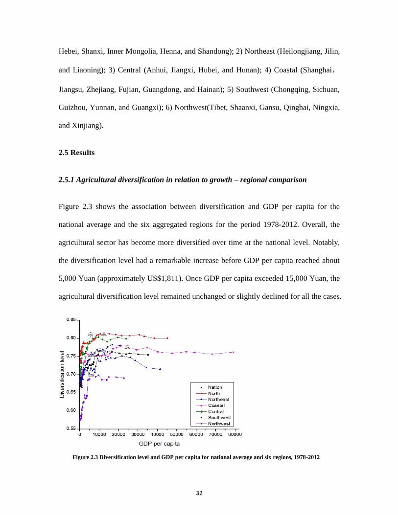
Figure 2.3 shows the association between diversification and GDP per capita for the
national average and the six aggregated regions for the period 1978-2012. Overall, the
agricultural sector has become more diversified over time at the national level. Notably,
the diversification level had a remarkable increase before GDP per capita reached about
5,000 Yuan (approximately US$1,811). Once GDP per capita exceeded 15,000 Yuan, the
agricultural diversification level remained unchanged or slightly declined for all the cases.
Figure 2.3 Diversification level and GDP per capita for national average and six regions, 1978-2012
33
Moreover, the diversification level decreased during 2003-2007 in most regions. This
decline could be partially explained by the nationwide policy effort to increase grain
production at the time. A series of policies were implemented to stimulate farmers’ grain
production and the relative profitability of grain production, when grain production
decreased by 16% between 1998 and 2003. These policies included ending agricultural
taxes; directing subsidy payments to grain producers; grain crop support price; input
subsidies for fertiliser and farm equipment; and increased investment in infrastructure
(Carter, Zhong, and Zhu 2012).
The above pro-grain government policies effectively encouraged grain production so that
the area planted with grain recovered to 1997 levels, and the share of grain’s output to the
agricultural sector rose (Liu et al. 2008). The decline of production diversification
between 2002 and 2007 was attributed to this grain production rise/concentration, as
grains (rice, wheat, and maize) account for more than 50% of crop production.
The patterns of China’s agricultural diversification support the view of Timmer (1997)
that agriculture tends to be more diversified at macro levels in the early stage of
development. China’s practice further suggests that government policy, in particular that
encouraging grain production, was effective in changing the degree of diversification at
the national and regional levels. Moreover, the degree of diversification varies among
regions at the same growth level/GDP per capita. Studies in other developing countries
indicate that besides the growth of GDP, agricultural diversification is closely related to
the degree of market development, especially the level of growth prior to agricultural
transformation, and the relative importance of agriculture in the region (Dorsey, Jarjoura,
and Rutecki 2005). This is true in the Chinese case; for example, the Northwest and
34
Southwest regions were at similar growth levels between 1978 and 2002, but the
Southwest region had a higher level of agricultural diversification owing to its
comparatively developed markets and infrastructure, and the intensification of the
piggery and feedstuff industries (Carter, Zhong, and Zhu 2012). By contrast, the
Northwest region has low agro-ecological potential (rainfall, soils, topography),
underdeveloped markets and infrastructure (isolated from demand centres and coastal
areas for exporting), and a higher share of agriculture in the region’s GDP. Consequently,
agriculture in this area is the least diversified among the six regions.
The comparisons above suggest that the rate of agricultural diversification is related to
comparative advantage (natural resources, access to markets), development levels
(education, access to information, markets) and the relative importance of agriculture in
the regions. For instance, the coastal region is the most developed area in China, with the
highest average GDP per capita (Figure 2.3). Production diversification levels in this
zone, however, are relatively low among the six regions. This can be explained by the
fact that the rapid urbanisation and industrialisation in this region has led to grain
production decline which, in turn, led to the importance of agriculture in the economy
diminishing relatively faster.
2.5.2 Agricultural transformation and its interdependence with non-agricultural sector
in underdeveloped regions – the case of Gansu province
Gansu Province is one of the poorest regions in China. In 2012, average rural per capita
income was 4,507 Yuan (the lowest in China), accounting for only 57% of the national
average 7,917 Yuan (NBSC 2013). In terms of agricultural conditions, Gansu is poorly
35
endowed with natural resources, one-fifth of the cultivated land is terraced, and annual
average rainfall ranges from 50 mm in the West to550 mm in the East (Gansu Yearbook
Editorial Board 2007-2011). Growth in Gansu’s agricultural sector has been not ably
slow, with low productivity. It accounts for 2.3% of China’s rural employment, but
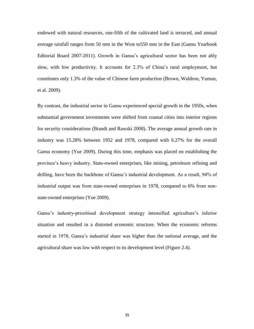
constitutes only 1.3% of the value of Chinese farm production (Brown, Waldron, Yuman,
et al. 2009).
By contrast, the industrial sector in Gansu experienced special growth in the 1950s, when
substantial government investments were shifted from coastal cities into interior regions
for security considerations (Brandt and Rawski 2008). The average annual growth rate in
industry was 15.28% between 1952 and 1978, compared with 6.27% for the overall
Gansu economy (Yue 2009). During this time, emphasis was placed on establishing the
province’s heavy industry. State-owned enterprises, like mining, petroleum refining and
drilling, have been the backbone of Gansu’s industrial development. As a result, 94% of
industrial output was from state-owned enterprises in 1978, compared to 6% from non-
state-owned enterprises (Yue 2009).
Gansu’s industry-prioritised development strategy intensified agriculture’s inferior
situation and resulted in a distorted economic structure. When the economic reforms
started in 1978, Gansu’s industrial share was higher than the national average, and the
agricultural share was low with respect to its development level (Figure 2.4).
36
Figure 2.4 Sectoral shares in GDP and employment, Gansu province and national average
(Sources: China Statistical Yearbook, and Gansu Yearbook, 1978-2012)
Consequently, Gansu experienced a catch-up growth period in agriculture between 1979
and 1985; the average farm labour productivity growth rate exceeded the industrial sector
(4.30% compared to -6.51%, Appendix Table 1), and the productivity gain was attributed
to the province-wide effort toward grain self-sufficiency (Yue 2009). The share of
agriculture in GDP started declining when labour started shifting to the industrial and
services sector after 1985, indicated by the declining agricultural employment (Figure
2.4).
The compositional distortion in Gansu’s economy before reforms and the later efforts to
optimise the industrial structure were reflected in its changing diversification patterns.
The degree of diversification in Gansu’s farming declined sharply when production was
focused on attaining grain self-sufficiency between 1978 and 1985 (Figure 2.5). Then,
another major decline took place during 1995-2003, which is consistent with the nation’s
37
overall change, explained by the widespread increase of grain production, as discussed
earlier.
Figure 2.5 Changing of agricultural diversification, China and Gansu province
The process of diversification in Gansu’s agricultural sector indicates that agricultural
diversification is affected by the non-agricultural sector and the process and progress of
structural change. The growth pathway provides some insights into how sectoral
composition in the early stage of transformation affects diversification in the rural
economy. Diversification in the agricultural sector may be constrained if farms cannot
move to higher productivity sectors, and agriculture’s share in employment stagnates.
This is supported by findings from Brandt, Hsieh, and Zhu (2008), suggesting that
provinces with a relatively large state sector at the start of reforms are likely to
experience slower growth. The present study shows that the capital intensive and low-

38
labour-absorbing state sector indeed posed higher initial barriers to Gansu’s rural labour
mobility, and subsequently delayed the pace of structural transfer and economic growth.
39
Chapter 3
The farm level production specialisation and commercialisation
3.1 Introduction
Chapter 2 reviewed China’s regional agricultural diversification under the framework of
structural change. The results show that the transformation of China’s agriculture is
similar to the stages of development from other countries; that is, China’s agricultural
sector becomes more diversified as the economy grows. The current chapter aims to
address the second hypothesis (H2) of this study, which is to ascertain the extent to which
farmers specialise in more profitable products in response to market demand.
The existing research has studied commercialisation and specialisation either as
interchangeable concepts for market participation, or separately whereby one factor
determines another. For example, Dorsey (1999) used commercialisation as an
explanatory variable in determining the pattern and extent of specialisation. A few other
studies treat specialisation as a factor affecting market participation (Gebreselassie and
Ludi 2007, Gebreselassie and Sharp 2008). Only a limited scope of research has
suggested, yet explicitly demonstrated, the interaction between householders’ market
participation and production specialisation. For instance, Wickramasinghe and
Weinberger(2013) stated that productivity changes stimulated by structural
transformation from subsistence to specialised production enable greater
commercialisation, while commercialisation encourages better use of comparatively
advantaged resources(apparently production specialisation is one of the cases).
40
The purpose of this study is to examine smallholders’ market participation in relation to
farm specialisation. It is proposed that macro-level agricultural transformation is
accompanied by farm specialisation, and that farm-level decisions on production
specialisation/diversification are conditioned to the degree of market participation. An in-
depth empirical study of the relationship between China’s small farmers’ market
participation and production specialisation explores factors which may determine how
specialisation and productivity growth can raise household incomes through greater
market participation. The findings of this research will advance our understanding of
issues pertaining to the structural change from subsistence to the more specialised and
market-oriented systems, and provide policy guidance on promoting smallholders’
market participation.
3.2 Theoretical foundations
The idea that there is a two-way relationship between specialisation and
commercialisation dates back to the classic Smithian account. It is noted that “the greatest
improvements in the productive powers of labour…seem to have been the effects of the
division of labour” (Smith, A, 1776, Book 1, Chapter1), and “it is the power of
exchanging that gives rise to the division of labour” (Book 1, Chapter 3). Yong (1928)
further explicitly states that division of labour depends on the extent of the market, but
the extent of market also depends upon the extent of the division of labour.
Theoretically, the link between market and specialisation can be explained as:
specialisation over tasks and products improves productivity, increases production and
supply, and in turn stimulates market participation (Wickramasinghe and Weinberger
41
2013, Emran and Shilpi 2012). Meanwhile larger markets ensure adequate demand for
large-scale production and higher profit for non-staple crops. Well-functioning markets
reduce transaction costs and provide traded inputs and promote sales of farm products.
The increasing opportunity costs of family labour, however, induce farmers to reduce
farm activities and concentrate production on a few enterprises to increase profitability
per unit (Timmer 1997, von Braun 1995, Pingali and Rosegrant 1995).
At the farm level, the link between householders’ market participation and specialisation
of production can be explained by transaction cost economics theory within the
agricultural household framework: as production specialises, unit costs of market
participation such as transportation and communication decline, while organizing
production associated costs rise because the increasing volume and consistency for
supply. In order to maximise household utility, farmers are assumed to makes optimal
decisions on how much to produce, consume, buy and sell, subject to income constraint,
production technology, resource constraints and non-tradable availability constraint
(Wickramasinghe and Weinberger ,2013).
Smallholders in developing countries are typically both producer and consumer, and
normally face missing or incomplete markets for inputs and output, including labour and
capital. As a result, their decisions on production, resource especially labour allocation
and consumption may be interdependent upon one another (Taylor and Adelman, 2002).
This classic household-farm-model provides an explanatory framework for an
interdependent relationship between smallholders’ market participation and production
specialisation.
42
3.3 The trend of the farm level specialisation
The concept of specialisation comes together with diversification. Farms are rarely
completely specialised, therefore, specialisation is often a matter of degree relative to
diversification. In more general terms, specialisation implies a limited scope of farm
production. Farmers specialise in the products they produce, or in the processes
performed to reduce the number of activities.
3.3.1 Measuring smallholders’ production specialisation
The Herfindahl index of product concentration was used to compute the farm level
specialisation index, the same calculation and interpretation as discussed in method 2.4.1
of Chapter 2.A total 14 categories of crops were included in the formulation: wheat,
maize, forage, buckwheat, millet, beans, potato, rapeseed, fruits, vegetables, melons,
seedlings, sunflower, Chinese herbs for different farms the number of crops produced
varies.
On average, farms were engaged in six different cropping activities across the study areas.
Both the commercialisation and specialisation indices are a continuum rather than binary
structures, therefore no absolute distinctions between “commercialised/specialised” and
“non-commercialised/specialised” farms are made in this study.
3.3.2 Study area
The study areas are located in Qingyang Prefecture, Gansu Province, in the Northwest of
China. Qingyang Prefecture is in eastern Gansu and accounts for approximately 10% of
the value of Gansu’s agricultural production and farm employment (Brown, Waldron, Liu,

43
et al. 2009). Farming systems in this region are mainly integrated crop-livestock systems
(Nolan et al. 2008, Hou et al. 2008). Farmers in the higher rainfall areas of the south
predominately grow wheat and maize, where farmers in the more arid northern areas
focus mainly on small ruminant livestock production (Nolan et al. 2008). In the central
part of the prefecture, mixed farming systems are more prevalent.
Table 3.1 shows the structural changes in Qingyang’s agricultural sector between 1995
and 2010.Overall, agriculture is no longer the dominant income source, as non-farm
earnings have become increasingly important to household livelihoods. Like elsewhere in
China, the relative importance of staple grain production has declined. Production of cash
crops and livestock has become more prevalent, but these are also more volatile.
Secondary data show that household income from farming decreased from about 66% in
1995 to 40% in 2010, with the exception of the increase in 2005(Qingyang Yearbook
1994-2011)7.
Table 3.1 Farm income composition and growth of selected commodities in Qingyang, 1995–2010
1995 2000 2005 2010
Farm income share:
Income from farm (%) 66.37 40.78 61.00 39.51
Wage-earning (%) 12.43 30.32 22.85 37.52
Other income (%) 21.20 28.90 16.15 22.97
Production, sown area, and yield:
Wheat:
Production (kt) 173.39 170.50 376.00 342.40
Area (kha) 196.51 205.25 162.92 130.12
Maize:
Production (kt) 142.40 159.00 294.10 604.60
Area (kha) 39.92 42.37 56.26 150.46
7This increase was due to a series of policies that were implemented to stimulate farmers’ grain production incentives
and the relative profitability of grain production, when grain production decreased by 16% between 1998 and 2003.
These policies included ending agricultural taxes, direct subsidy payments to grain producers, grain crop support price,
input subsidies for fertiliser and farm equipment, and increased investment in infrastructure (Carter, Zhong, and Zhu
2012).
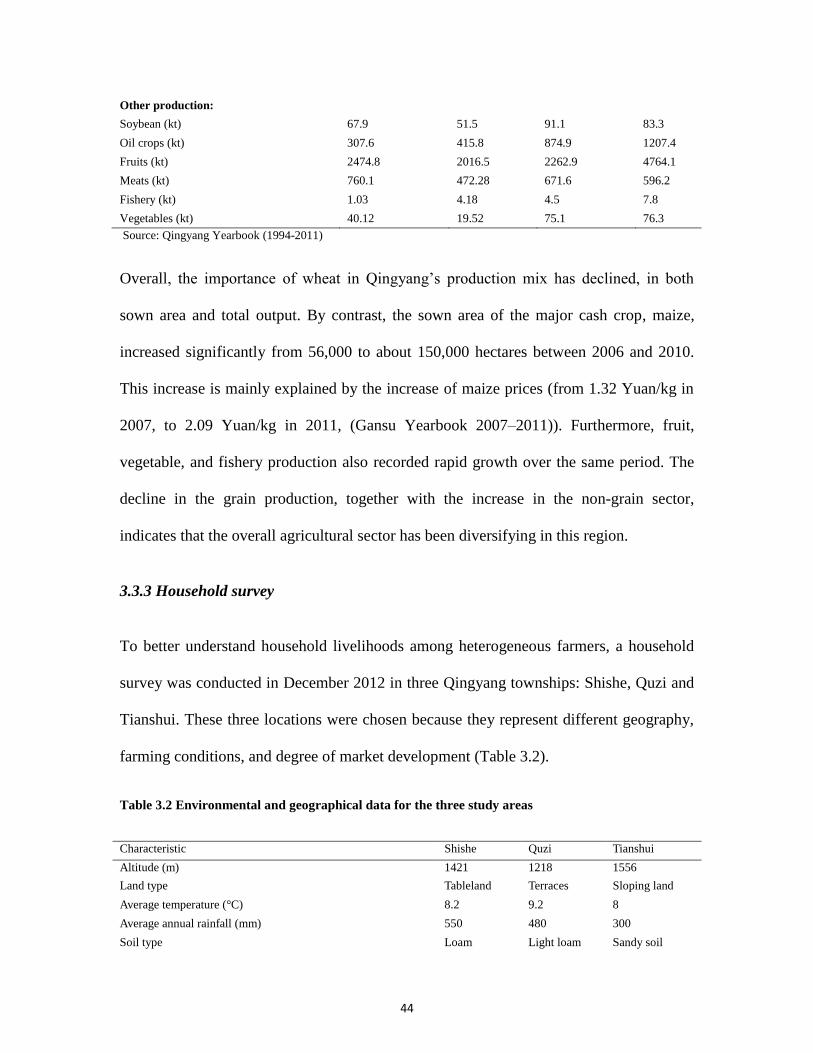
44
Other production:
Soybean (kt) 67.9 51.5 91.1 83.3
Oil crops (kt) 307.6 415.8 874.9 1207.4
Fruits (kt) 2474.8 2016.5 2262.9 4764.1
Meats (kt) 760.1 472.28 671.6 596.2
Fishery (kt) 1.03 4.18 4.5 7.8
Vegetables (kt) 40.12 19.52 75.1 76.3
Source: Qingyang Yearbook (1994-2011)
Overall, the importance of wheat in Qingyang’s production mix has declined, in both
sown area and total output. By contrast, the sown area of the major cash crop, maize,
increased significantly from 56,000 to about 150,000 hectares between 2006 and 2010.
This increase is mainly explained by the increase of maize prices (from 1.32 Yuan/kg in
2007, to 2.09 Yuan/kg in 2011, (Gansu Yearbook 2007–2011)). Furthermore, fruit,
vegetable, and fishery production also recorded rapid growth over the same period. The
decline in the grain production, together with the increase in the non-grain sector,
indicates that the overall agricultural sector has been diversifying in this region.
3.3.3 Household survey
To better understand household livelihoods among heterogeneous farmers, a household
survey was conducted in December 2012 in three Qingyang townships: Shishe, Quzi and
Tianshui. These three locations were chosen because they represent different geography,
farming conditions, and degree of market development (Table 3.2).
Table 3.2 Environmental and geographical data for the three study areas
Characteristic Shishe Quzi Tianshui
Altitude (m) 1421 1218 1556
Land type Tableland Terraces Sloping land
Average temperature (°C) 8.2 9.2 8
Average annual rainfall (mm) 550 480 300
Soil type Loam Light loam Sandy soil
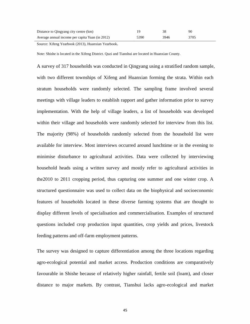
45
Distance to Qingyang city centre (km) 19 38 90
Average annual income per capita Yuan (in 2012) 5390 3946 3705
Source: Xifeng Yearbook (2013), Huanxian Yearbook.
Note: Shishe is located in the Xifeng District. Quzi and Tianshui are located in Huanxian County.
A survey of 317 households was conducted in Qingyang using a stratified random sample,
with two different townships of Xifeng and Huanxian forming the strata. Within each
stratum households were randomly selected. The sampling frame involved several
meetings with village leaders to establish rapport and gather information prior to survey
implementation. With the help of village leaders, a list of households was developed
within their village and households were randomly selected for interview from this list.
The majority (98%) of households randomly selected from the household list were
available for interview. Most interviews occurred around lunchtime or in the evening to
minimise disturbance to agricultural activities. Data were collected by interviewing
household heads using a written survey and mostly refer to agricultural activities in
the2010 to 2011 cropping period, thus capturing one summer and one winter crop. A
structured questionnaire was used to collect data on the biophysical and socioeconomic
features of households located in these diverse farming systems that are thought to
display different levels of specialisation and commercialisation. Examples of structured
questions included crop production input quantities, crop yields and prices, livestock
feeding patterns and off-farm employment patterns.
The survey was designed to capture differentiation among the three locations regarding
agro-ecological potential and market access. Production conditions are comparatively
favourable in Shishe because of relatively higher rainfall, fertile soil (loam), and closer
distance to major markets. By contrast, Tianshui lacks agro-ecological and market

46
potential, while Quzi is geographically and economically between the other two locations,
as shown in Figure 3.1.
Figure3.1 LocationsoftheThreeCaseStudyAreas
Table3.3 summarises the farm characteristics of the surveyed farms in the three study
areas. The results show that farms in Shishe have the lowest average land-labour ratios
(0.11, compared to 0.17 and 0.68 for Quzi and Tianshui, respectively) and cropped areas
(0.50, over 0.85 and 3.44 for Quzi and Tianshui, respectively). Shishe households are the
least active in crop and livestock production, engaging in the smallest number of
livestock and crop enterprises. However, farmland is more consolidated and divided into
fewer plots in this district (number of plots are 2.8, 5.2, and 5.5 for Shishe, Quzi and
Tianshui, respectively). Furthermore, Shishe incomes (on-farm, off-farm, and total
income per capita) and yield for both grain (wheat) and cash crops are highest among the
three locations. Additionally, although it is not statistically significant, Shishe farms tend
to have relatively higher fertiliser input and hire more farm labour.

47
Quzi has both productive river valleys that are suitable for cropping production and
terraced slopes for livestock grazing, perennial crops, and trees. Thus, farmers in Quzi
tend to integrate with crop-livestock production, and farm productivity is higher than in
Tianshui.
Table 3.3 Farm characteristics of the surveyed farms in the three study areas
Items Shishe
(N=120)
Quzi
(N=94)
Tianshui
(N=103)
F statistic Land-labour ratio (people/ha) 0.11(0.01) 0.17(0.12) 0.68(0.347) 225.9**
Cultivated area (ha) 0.50(4.33) 0.85(9.6) 3.44(27.5) 225.2**
Wheat yield (Kg/ha) 4341(2176) 3467(1905) 1126(964) 73.57**
Number of plots 2.8(1.6) 5.2(3.1) 5.6(3.4) 35.8**
Number of livestock (Type) 0.25(1.26) 0.94(2.23) 1.35(0.88) 14.8**
Number of crops grown 2.4(2.13) 2.7 (3.1) 3.9 (2.74) 57.194**
Off-farm income (Yuan) 24513(24706) 16701(20416) 17804(23938) 3.648*
Total income (Yuan) 46525(37987) 29273(23343) 30228(29260) 10.63**
Income per capita( Yuan/person) 9368(7166) 5810(5422) 5680(5306) 13.143**
Migrants(Persons) 1.23(1.18) 0.93(0.9) 0.87(0.77) 4.4*
Total labour input (man-days/farm) 169.6(237) 199.9(135) 258.4(166) 6.16**
Hired labour (man-days/farm) 11.8(114) 3.0(9.2) 1.5(9.2) 0.49
Machinery cost (Yuan/farm) 504(385) 538(499) 249(566) 10.88**
Fertiliser applied (Yuan/farm) 1591(1877) 1327(995) 1450(974) 0.95
Land productivity (Yuan/ha) 21000(2025) 16785(2109) 4920(754) 10.91**
Note: 6.285 Yuan = 1 US$ at the survey time; *and ** indicate significance at 1% and 5% respectively; figures in
parentheses are standard errors.
By contrast, Tianshui farmers use more labour in farm activities, with a relative focus on
livestock production. Productivity in Tianshui is particularly low compared to the other
two. For example, wheat yields were 1,126 kg/ha (compared with 4,341 kg/ha and 3,467
kg/ha in Shishe and Quzi, respectively), and its overall land productivity is only about a
quarter of that for Shishe and Quzi (4,920 Yuan/ha, compared to 21,000 and 16,785
Yuan/ha, respectively).
Figure 3.2 below shows the relationship between specialisation and income per capita for
all surveyed farms across the three study areas. Overall, the level of specialisation is
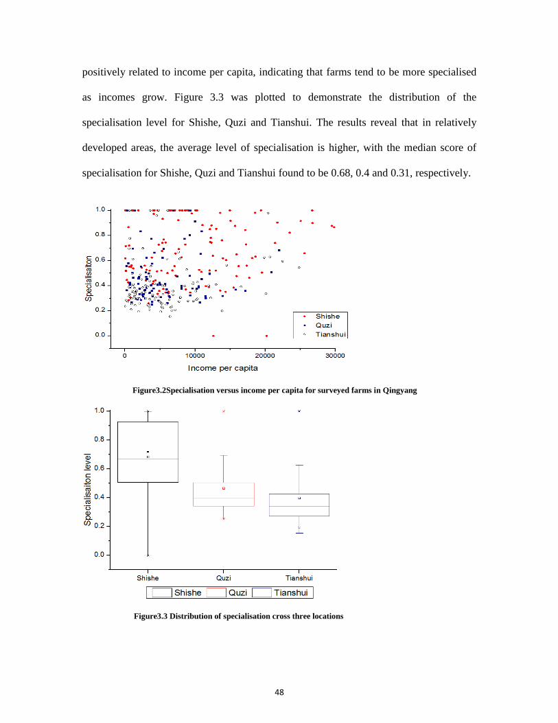
48
positively related to income per capita, indicating that farms tend to be more specialised
as incomes grow. Figure 3.3 was plotted to demonstrate the distribution of the
specialisation level for Shishe, Quzi and Tianshui. The results reveal that in relatively
developed areas, the average level of specialisation is higher, with the median score of
specialisation for Shishe, Quzi and Tianshui found to be 0.68, 0.4 and 0.31, respectively.
Figure3.2Specialisation versus income per capita for surveyed farms in Qingyang
Figure3.3 Distribution of specialisation cross three locations
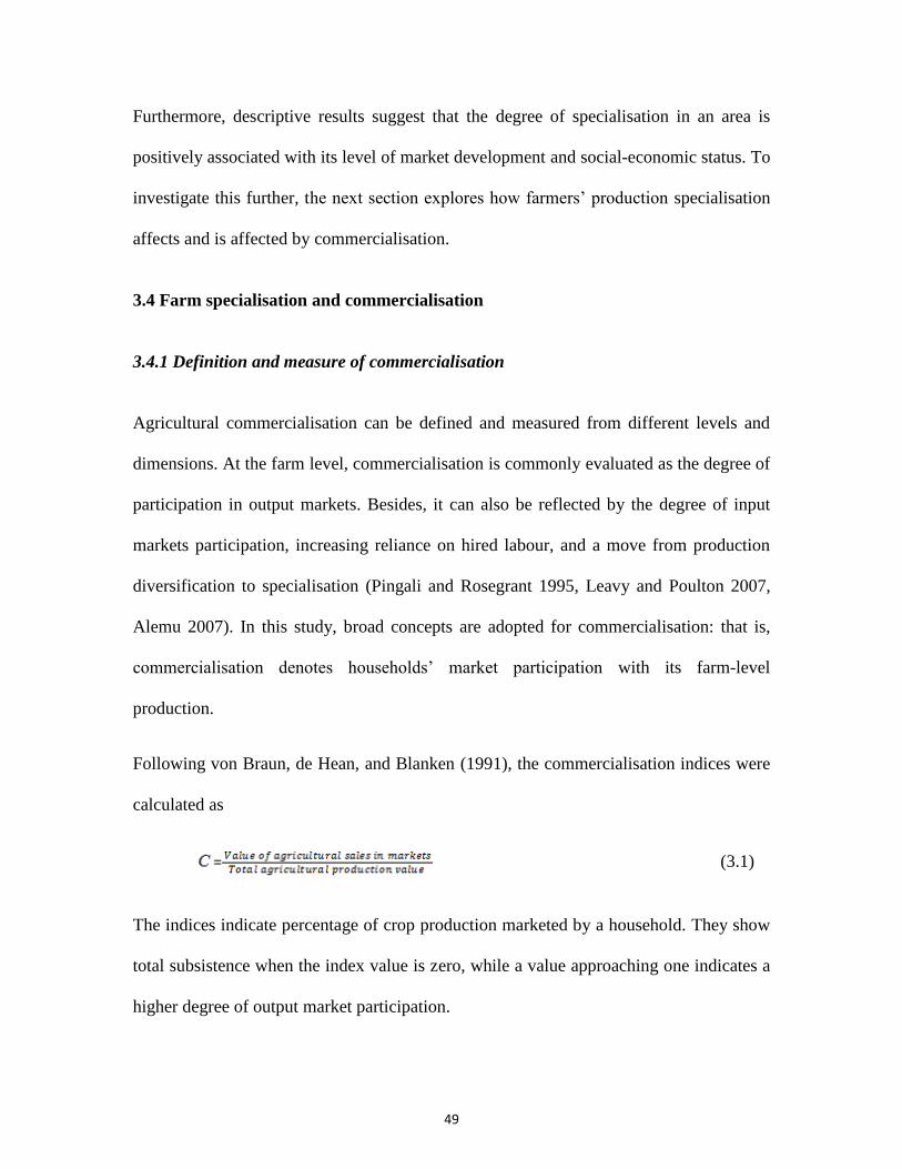
49
Furthermore, descriptive results suggest that the degree of specialisation in an area is
positively associated with its level of market development and social-economic status. To
investigate this further, the next section explores how farmers’ production specialisation
affects and is affected by commercialisation.
3.4 Farm specialisation and commercialisation
3.4.1 Definition and measure of commercialisation
Agricultural commercialisation can be defined and measured from different levels and
dimensions. At the farm level, commercialisation is commonly evaluated as the degree of
participation in output markets. Besides, it can also be reflected by the degree of input
markets participation, increasing reliance on hired labour, and a move from production
diversification to specialisation (Pingali and Rosegrant 1995, Leavy and Poulton 2007,
Alemu 2007). In this study, broad concepts are adopted for commercialisation: that is,
commercialisation denotes households’ market participation with its farm-level
production.
Following von Braun, de Hean, and Blanken (1991), the commercialisation indices were
calculated as
(3.1)
The indices indicate percentage of crop production marketed by a household. They show
total subsistence when the index value is zero, while a value approaching one indicates a
higher degree of output market participation.
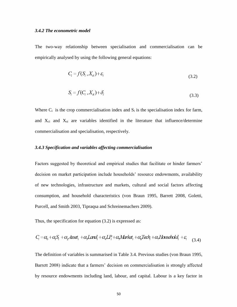
50
3.4.2 The econometric model
The two-way relationship between specialisation and commercialisation can be
empirically analysed by using the following general equations:
(3.2)
(3.3)
Where Ci is the crop commercialisation index and Si is the specialisation index for farm,
and Xci and Xsi are variables identified in the literature that influence/determine
commercialisation and specialisation, respectively.
3.4.3 Specification and variables affecting commercialisation
Factors suggested by theoretical and empirical studies that facilitate or hinder farmers’
decision on market participation include households’ resource endowments, availability
of new technologies, infrastructure and markets, cultural and social factors affecting
consumption, and household characteristics (von Braun 1995, Barrett 2008, Goletti,
Purcell, and Smith 2003, Tipraqsa and Schreinemachers 2009).
Thus, the specification for equation (3.2) is expressed as:
(3.4)
The definition of variables is summarised in Table 3.4. Previous studies (von Braun 1995,
Barrett 2008) indicate that a farmers’ decision on commercialisation is strongly affected
by resource endowments including land, labour, and capital. Labour is a key factor in
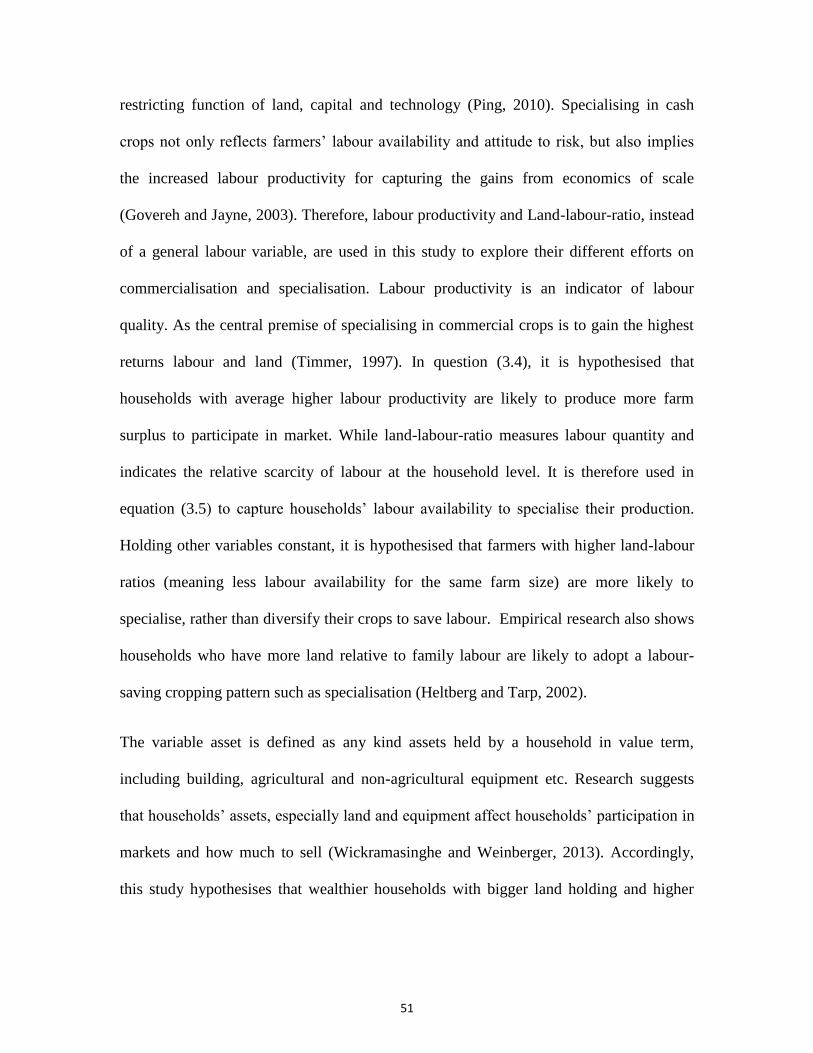
51
restricting function of land, capital and technology (Ping, 2010). Specialising in cash
crops not only reflects farmers’ labour availability and attitude to risk, but also implies
the increased labour productivity for capturing the gains from economics of scale
(Govereh and Jayne, 2003). Therefore, labour productivity and Land-labour-ratio, instead
of a general labour variable, are used in this study to explore their different efforts on
commercialisation and specialisation. Labour productivity is an indicator of labour
quality. As the central premise of specialising in commercial crops is to gain the highest
returns labour and land (Timmer, 1997). In question (3.4), it is hypothesised that
households with average higher labour productivity are likely to produce more farm
surplus to participate in market. While land-labour-ratio measures labour quantity and
indicates the relative scarcity of labour at the household level. It is therefore used in
equation (3.5) to capture households’ labour availability to specialise their production.
Holding other variables constant, it is hypothesised that farmers with higher land-labour
ratios (meaning less labour availability for the same farm size) are more likely to
specialise, rather than diversify their crops to save labour. Empirical research also shows
households who have more land relative to family labour are likely to adopt a labour-
saving cropping pattern such as specialisation (Heltberg and Tarp, 2002).
The variable asset is defined as any kind assets held by a household in value term,
including building, agricultural and non-agricultural equipment etc. Research suggests
that households’ assets, especially land and equipment affect households’ participation in
markets and how much to sell (Wickramasinghe and Weinberger, 2013). Accordingly,
this study hypothesises that wealthier households with bigger land holding and higher
52
average labour productivity have declining demand for subsistence production, and are
more likely to sell their surplus into markets.
The development level of technologies and markets, captured by Tech (fertiliser) and
location dummy variables, respectively, are expected to affect households’ decisions on
commercialisation. Adoption of new production technologies can increase agricultural
productivity because of the reduction of per unit costs. Households are therefore in a
better position of net marketable surplus; this, in turn, affects their market participation
choices. Besides, research has proven there are strong associations between households’
market access and the level of commercialisation (von Braun 1995, Barrett 2008). Poor
market and infrastructure conditions raise transaction costs that substantially hinder
production and market participation decisions. In the current research, the market access
is indicated by the two dummy variables of Dummy-Shishe and Dummy-Tianshui.
Shishe is closer to the central market and has better biophysical potential and marketing
options compared to Quzi. On the other hand, both production conditions and access to
markets in Tianshui are less favoured compared with Quzi.
The vector i is to capture the influence of household characteristics on
commercialisation, including data on head gender, household head’s schooling (years)
and farm experience (years). Those households’ characteristics are considered
endogenous when related to decision-making regarding production, consumption, and
resource allocation. For example, different gender and age groups have different
preferences in income and time allocation, which may affect households’ level of market
participation.
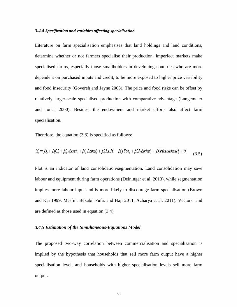
53
3.4.4 Specification and variables affecting specialisation
Literature on farm specialisation emphasises that land holdings and land conditions,
determine whether or not farmers specialise their production. Imperfect markets make
specialised farms, especially those smallholders in developing countries who are more
dependent on purchased inputs and credit, to be more exposed to higher price variability
and food insecurity (Govereh and Jayne 2003). The price and food risks can be offset by
relatively larger-scale specialised production with comparative advantage (Langemeier
and Jones 2000). Besides, the endowment and market efforts also affect farm
specialisation.
Therefore, the equation (3.3) is specified as follows:
(3.5)
Plot is an indicator of land consolidation/segmentation. Land consolidation may save
labour and equipment during farm operations (Deininger et al. 2013), while segmentation
implies more labour input and is more likely to discourage farm specialisation (Brown
and Kai 1999, Mesfin, Bekabil Fufa, and Haji 2011, Acharya et al. 2011). Vectors and
are defined as those used in equation (3.4).
3.4.5 Estimation of the Simultaneous-Equations Model
The proposed two-way correlation between commercialisation and specialisation is
implied by the hypothesis that households that sell more farm output have a higher
specialisation level, and households with higher specialisation levels sell more farm
output.
54
The simultaneity problem arises because the values of these two endogenous variables
are jointly determined in a simultaneous-equations system. In this case, ordinary least
squares (OLS) estimators would be inefficient and inconsistent (Lin and Shao 2000). In
addition, the application of the order condition to the simultaneous equations (3.4) and
(3.5) reveals that both equations are over-identified, implying that the simultaneous
model as a whole is over-identified, which further suggests that the OLS method is not
the appropriate method to use(Gujarati 2008).
Both simultaneity and over-identification problems suggest that the methods to use are
either the two-stage least squares (2SLS) or three-stage least squares (3SLS). It is more
likely in the cases used that some unconsidered factors influencing commercialisation
could also affect specialisation, that is, the error terms i and i may be correlated. If
this is true, then the single equation estimation of 2SLS could also be inappropriate and
inefficient. The system estimates made by 3SLS is supposed to produce more efficient
estimates than 2SLS. This is because by using Generalised Least Squares (GLS) methods,
3SLSentails simultaneous solution of all equations and incorporates the additional
correction for heteroscedasticity to 2SLS.However, as a norm and as a comparison of
some of the approaches, the three methods of OLS, 2SLS and 3SLS are presented in this
study.
In specifying the2SLS and 3SLS estimators, it is critical to obtain valid instruments for
the endogenous variables. The valid instruments should be relevant, uncorrelated with the
error term and correctly excluded from the estimated equations(Rios et al. 2009). The
possible instruments in this study are land productivity and elderly (number of elderly
people in the household).Literature on small farm commercialisation suggests there is a
55
strong association between households’ farm productivity and market participation
(Barrett, 2008).The rationale for choosing the variable elderly to serve as an instrument
for crop specialisation is that most of the specialised farm production, such as orchard,
tends to be run or supervised by elderly people with hired labour (Li et al. 2013).
Therefore, the availability of elderly family labour is assumed to be related to the
specialisation decision, but not with other exogenous variables and the error term.
The validity, relevance, and strength of the two instruments identified, as well as the
endogeneity of the commercialisation and specialisation variables, are tested using a
serial diagnostics approach. The results of the Sargan statistic for over-identifying
restrictions, the Stock-Yogo weak instrument test, and the Durbin-Wu-Hausman test are
reported as part of post estimation tests (Tables 3.6 and 3.7).First, the endogeneity of
commercialisation and specialisation is confirmed by the Durbin-Wu-Hausman test (both
P<0.01), showing an instrumental-variables estimator is necessary. Second, in the first-
stage 2SLS regression, the statistically significant coefficients of land-productivity on
commercialisation ( =0.00003, P<0.01) and elderly on specialisation ( =-0.03,
P < 0.001)have reasonable explanatory power over the relevance of those two
instruments (second section of Tables 3.6 and 3.7).Third, the validity of the instruments
is confirmed by the over-identification tests: the J-statistics is 0.86 with a p-value of 0.64
in the commercialisation regression, and J-statistics of1.104 (p=0.5769) in the
specialisation regression. This result indicates that the error terms are uncorrelated with
the instruments, implying that the instruments are valid. Fifth, land-productivity and
elderly are verified to be reasonably strong instruments, as the F statistic for the joint
significance of the instruments excluded from the structural model are 38.49 and 15.94,
56
respectively, which are much larger than the rule of thumb value of 10.The strength of
the instruments can be further verified by the reported minimum eigen value statistics
exceeding the Stock-Yogo critical values for 10% maximal size and 5% maximal bias.
The descriptive statistics of the variables included in the study, and the corresponding
correlation matrix of the variables, are shown in Tables 3.4 and Table 3.5.All the
correlation coefficients are smaller than 0.5 (commonly accepted level is 0.7 in social
sciences studies), suggesting that the individual coefficient estimates of the remaining
exogenous variables are not affected by the multicollinearity problem8.
3.5 Results and discussion
The estimation results using the OLS, 2SLS and 3SLS methods are summarised in Tables
3.6 and 3.7. Compared to 2SLS and 3SLS techniques, the OLS estimation yields either
insignificance correlation between the hypothesised specialisation and commercialisation,
or produces signs that are contrary to what is expected for control variables such as Land,
Head-schooling, Dummy-Shishe and Head-gender. These unexpected signs and less
significance of coefficients may be attributed to the simultaneous-equation bias,
indicating the inappropriateness of the OLS method in the system equations.
By contrast, all 3SLS and 2SLS estimates correspond to the theoretical expectations or
turn out sensible results. In particular, both of the estimators confirm a strong two-way
correlation between specialisation and commercialisation. Overall, there is little
difference in the estimates of the two methods. The closeness of the value of the
82SLS and 3SLS methods reduce the endogenous variables’ collinearity with the remaining independent variables, but
do not preclude the possibility of collinearity between the exogenous variables.

57
parameter estimates implies that i and i in equations 3.4 and 3.5 might be uncorrelated.
Since 3SLS is generally consistent and more efficient than 2SLS asymptotically
(Cameron and Trivedi, 2010), the following discussion of results is based on3SLS
estimates.
The strong interrelationship between specialisation and commercialisation supports the
main hypothesis of this study; that is, the specialisation affect, and is also affected by
commercialisation. Specifically, the results imply that households that sell more farm
output have a higher specialisation level, and households with higher specialisation levels
sell more farm output. For the studied smallholders, this jointly-determined correlation
between commercialisation and specialisation denotes that farm production is
concentrated towards market-oriented activities, rather than on the production of a larger
range of farm products for subsistence purposes.
Households’ capital asset is negatively associated with crop commercialisation, but
positively related to specialisation. This means that households in a relatively advantaged
financial position are more likely to specialise in crop production, but sell less of their
output. The result, however, does not hold true when using total income and/or income
per capita as dependent variables, with insignificant effect as well as opposite sign (see
Table 3.8). The puzzle and inconsistency of the influence of income and asset holding on
commercialisation, however, is in line with a study by Muriithi and Matz( 2015), which
find that households’ income and asset holdings have different impact on
commercialisation.Investigating effects of vegetable commercialisation on Kenyan
smallholders’ welfare, their results show commercialisation is positively associated with
income per capita, but no evidence for a positive association with asset holdings. They
58
speculate that households’ income is not necessarily used for farm investment or asset
accumulation. In fact, studies on this issue are controversial and the results are
inconclusive (Muriithi and Matz, 2015). A possible reason is that the definition/concept
of household assets is often vaguely defined and the scope of asset holdings varies in
different research settings. For example, productive assets, household income and wealth
are all used but not distinguished from one of each other, but vaguely indicated to be
associated with smallholders’ market participation (Michelson, 2013, Von Braun, 1995).
The literature on small farm market participation, however, suggests that households’
asset holdings have a positive effort on commercialisation, and that wealthier households
appear more likely to sell to the market than are other households (Barrett, 2008). This
existing literature is based on a broad context, in which market
participation/commercialisation is conceptually considered either equivalent or
exchangeable to specialisation. The current study, however, argues that farmers’
decisions on farm commercialisation and production specialisation are actually separate
and interacting. The empirical analyses distinguish and confirm that commercialisation
and specialisation are two different decisions; thus providing insights on how these two
activities react to each other, and how these processes respond differently to other
exogenous factors.
This research further suggests that capital asset holdings have different influences over
farmers’ market participation and decisions to specialise. The findings cast light on the
farm market participation theory by emphasising that higher asset endowments indeed
enable small farmers, who possess higher value of assets such as building and equipment
seem to lack the incentives to sell farm surplus. The possible reason could be that asset
59
holdings are more likely to relax credit constraints (such as equipment can service as
collateral in some cases) for households’ relatively long-term investment, rather than
generating cash by selling farm products (Goetz and Stephen, 1993). As von Braun (2008,
p189) points out, “some factors have more immediate effects on farmers’ decisions to
become more integrated in the market, whereas others may only have long-term effects”.
Indeed, it is intuitive that farmers with higher liquid assets are more likely to lack the
incentives to sell farm surplus. These farmers are more inclined to consider some longer-
term investments and technology adoption, such as embarking on production
specialisation, since wealthier farms are considered to be less risk-averse (Mesfin et al.
2011b), or are capable of taking more risks.
In terms of other factors affecting farmers’ decisions on commercialisation and
specialisation, most of the results are consistent with the theoretical assumptions and
previous empirical studies. For example, the finding that higher farm productivity and
new technologies significantly promote market participation, are similar to the findings of
Barrett (2008) and von Braun (2008).They found that the interaction between technology
adoption and increasing farm productivity directly increases the marketable surplus,
which is followed by the expansion of commercialisation.
Land-holding is found to be significantly negatively associated with specialisation, but an
insignificant factor to commercialisation. Previous empirical studies show that smaller
farmers are more likely to adopt new crops or technologies (von Braun,
2008).Furthermore, farmers’ decisions to specialise is hindered by land segmentation as
indicated by the negative and significant coefficient of plot against specialisation. This
outcome is consistent with the finding of Mesfin, Fufa, and Haji (2011),that a negative
60
relationship exists between the number of operational plots and crop specialisation.
Location dummies and household characteristics (head’s gender, schooling and farm
experience) are found to have no correlation with the farmers’ decisions on specialisation
and commercialisation. The insignificant result of market on commercialisation and
specialisation is unexpected, perhaps indicating that the location dummies used in the
model were unable to capture the variations of households’ access to market.
Unfortunately, the information regarding the distance of each individual household to
markets was not available in this study. If available, the difference in transaction cost
amongst households could be captured, allowing the influence of market and
specialisation to be ascertained.
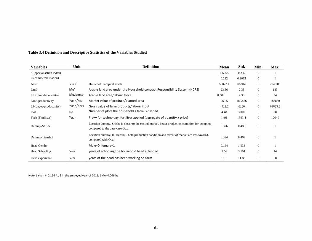
61
Table 3.4 Definition and Descriptive Statistics of the Variables Studied
Note:1 Yuan 0.156 AU$ in the surveyed year of 2011; 1Mu=0.066 ha
Variables Unit Definition Mean Std.
deviati
on
Min. Max.
Si (specialisation index) 0.6055 0.239 0 1
Ci(commercialisation)
index)
0.232 0.3015 0 1
Asset Yuan* Household’s capital assets 55872.4 182462 0 2.6e+06
Land Mu* Arable land area under the Household contract Responsibility System (HCRS) 23.86 2.38 0 143
LLR(land-labor-ratio) Mu/perso
n
Arable land area/labour force 0.503 2.38 0 34
Land-productivity Yuan/Mu Market value of produce/planted area 969.5 1802.56 0 188850
LP(Labor-productivity) Yuan/pers
on
Gross value of farm products/labour input 4411.2 6160 0 62833.3
Plot No. Number of plots the household’s farm is divided
4.48 3.007 0 28
Tech (Fertiliser) Yuan Proxy for technology, fertiliser applied (aggregate of quantity x price) 1491 1393.4 0 12040
Dummy-Shishe Location dummy. Shishe is closer to the central market, better production condition for cropping,
compared to the base case Quzi 0.376 0.486 0 1
Dummy-Tianshui Location dummy. In Tianshui, both production condition and extent of market are less favored,
compared with Quzi 0.324 0.469 0 1
Head Gender Male=0, female=1 0.154 1.533 0 1
Head Schooling Year years of schooling the household head attended 5.66 3.104 0 14
Farm experience Year years of the head has been working on farm 31.51 11.88 0 68
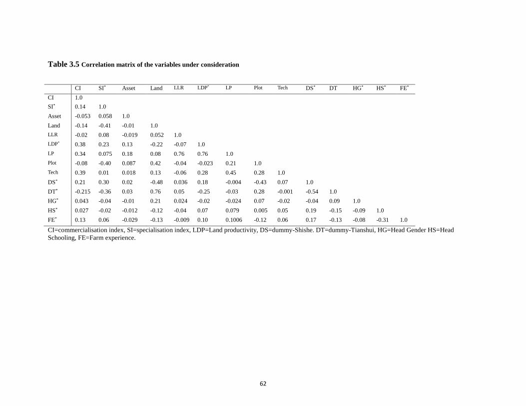
62
Table 3.5 Correlation matrix of the variables under consideration
CI SI* Asset Land LLR LDP* LP Plot Tech DS* DT HG* HS* FE*
CI 1.0
SI* 0.14 1.0
Asset -0.053 0.058 1.0
Land -0.14 -0.41 -0.01 1.0
LLR -0.02 0.08 -0.019 0.052 1.0
LDP* 0.38 0.23 0.13 -0.22 -0.07 1.0
LP 0.34 0.075 0.18 0.08 0.76 0.76 1.0
Plot -0.08 -0.40 0.087 0.42 -0.04 -0.023 0.21 1.0
Tech 0.39 0.01 0.018 0.13 -0.06 0.28 0.45 0.28 1.0
DS* 0.21 0.30 0.02 -0.48 0.036 0.18 -0.004 -0.43 0.07 1.0
DT* -0.215 -0.36 0.03 0.76 0.05 -0.25 -0.03 0.28 -0.001 -0.54 1.0
HG* 0.043 -0.04 -0.01 0.21 0.024 -0.02 -0.024 0.07 -0.02 -0.04 0.09 1.0
HS* 0.027 -0.02 -0.012 -0.12 -0.04 0.07 0.079 0.005 0.05 0.19 -0.15 -0.09 1.0
FE* 0.13 0.06 -0.029 -0.13 -0.009 0.10 0.1006 -0.12 0.06 0.17 -0.13 -0.08 -0.31 1.0
CI=commercialisation index, SI=specialisation index, LDP=Land productivity, DS=dummy-Shishe. DT=dummy-Tianshui, HG=Head Gender HS=Head
Schooling, FE=Farm experience.
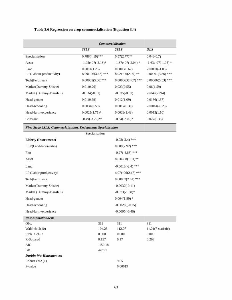
63
Table 3.6 Regression on crop commercialisation (Equation 3.4)
Commercialisation
3SLS 2SLS OLS
Specialisation 0.788(4.19)*** 0.57(2.77)** 0.048(0.7)
Asset -1.95e-07(-2.18)* -1.87e-07(-2.04) *
***
-1.63e-07(-1.95) *
Land 0.0014(1.25) 0.0006(0.62) -0.0001(-1.05)
LP (Labour productivity) 8.09e-06(3.62) ***
*** ***
8.92e-06(2.90) ** 0.00001(3.86) ***
Tech(Fertiliser) 0.00005(5.00)*** 0.000063(4.67) *** 0.00006(5.33) ***
Market(Dummy-Shishe) 0.01(0.26) 0.023(0.55) 0.06(1.59)
Market (Dummy-Tianshui) -0.034(-0.61) -0.035(-0.61) -0.049(-0.94)
Head-gender 0.01(0.99) 0.012(1.09) 0.0136(1.37)
Head-schooling 0.0034(0.59) 0.0017(0.30) -0.0014(-0.28)
Head-farm-experience 0.0025(1.71)* 0.0022(1.43) 0.0015(1.10)
Constant -0.49(-3.22)** -0.34(-2.09)* 0.027(0.33)
First Stage 2SLS: Commercialisation, Endogenous Specialisation
Specialisation
Elderly (Instrument) -0.03(-2.4) ***
LLR(Land-labor-ratio) 0.009(7.92) ***
Plot -0.27(-4.68) ***
Asset 8.83e-08(1.81)**
Land -0.0018(-2.4) ***
LP (Labor productivity) 4.07e-06(2.47) ***
Tech(Fertiliser) 0.00002(2.61) ***
Market(Dummy-Shishe) -0.0037(-0.11)
Market (Dummy-Tianshui) -0.073(-1.88)*
Head-gender 0.004(1.89) *
Head-schooling -0.0028((-0.75)
Head-farm-experience -0.0005(-0.46)
Post-estimation/tests
Obs. 311 311 311
Wald chi 2(10) 104.28 112.07 11.01(F statistic)
Prob. > chi 2 0.000 0.000 0.000
R-Squared 0.157 0.17 0.268
AIC -150.18
BIC -67.91
Durbin-Wu-Hausman test
Robust chi2 (1) 9.65
P-value 0.00019
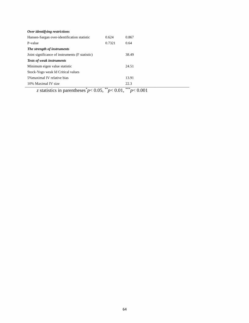
64
Over identifying restrictions
Hansen-Sargan over-identification statistic 0.624 0.867
P-value 0.7321 0.64
The strength of instruments
Joint significance of instruments (F statistic)
statistic)
38.49
Tests of weak instruments
Minimum eigen value statistic 24.51
Stock-Yogo weak Id Critical values
5%maximal IV relative bias 13.91
10% Maximal IV size 22.3
z statistics in parentheses*p< 0.05, **p< 0.01, ***p< 0.001
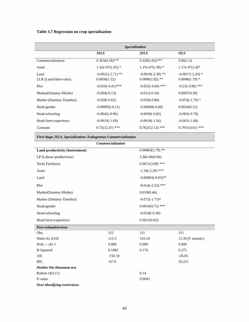
65
Table 3.7 Regression on crop specialisation
Specialisation
3SLS 2SLS OLS
Commercialisation 0.363(4.18)*** 0.328(3.65)*** 0.06(1.5)
Asset 1.32e-07(1.92) * 1.37e-07(1.96) * 1.17e-07(1.8)*
Land -0.0021(-2.71) ** -0.0019(-2.39) ** -0.0017(-2.24) *
LLR (Land-labor-ratio) 0.0056(1.52) 0.0096(1.82) ** 0.0088(1.79) *
Plot -0.019(-4.41)*** -0.022(-4.60) *** -0.23(-4.98) ***
Market(Dummy-Shishe) -0.004(-0.13) -0.011(-0.34) 0.0097(0.30)
Market (Dummy-Tianshui) -0.028(-0.62) -0.039(-0.86) -0.074(-1.76) *
Head-gender -0.00095(-0.11) -0.00068(-0.08) 0.0024(0.31)
Head-schooling -0.0042(-0.96) -0.0036(-0.82) -0.003(-0.78)
Head-farm-experience -0.0019(-1.69) -0.0018(-1.56) -0.001(-1.08)
Constant 0.75(12.47) *** 0.762(12.53) *** 0.797(14.01) ***
First Stage 2SLS, Specialisation: Endogenous Commercialisation
Commercialisation
Land-productivity (Instrument) 0.00003(1.79) **
LP (Labour productivity) 3.36e-06(0.66)
Tech( Fertiliser) 0.0075(3.89) ***
Asset -1.34(-2.29) ***
Land -0.00003(-0.05)**
Plot -0.014(-3.32) ***
Market(Dummy-Shishe) 0.019(0.44)
Market (Dummy-Tianshui) -0.072(-1.75)*
Head-gender 0.0014(4.75) ***
Head-schooling -0.014((-0.30)
Head-farm-experience 0.0011(0.82)
Post-estimation/tests
Obs. 311 311 311
Wald chi 2(10) 115.3 310.24 11.39 (F statistic)
Prob. > chi 2 0.000 0.000 0.000
R-Squared 0.1882 0.176 0.275
AIC -150.18 -26.05
BIC -67.9 56.221
Durbin-Wu-Hausman test
Robust chi2 (1) 8.14
P-value 0.0043
Over identifying restrictions

66
Hansen-Sargan over-identification statistic 0.624 1.104
0.1365 0.5769
The strength of instruments
Shea’s partial R2
Joint significance of instruments (F statistic) 15.91
Tests of weak instruments
Minimum eigen value statistic 30.34
Stock-Yogo weak ID test
5%maximal IV relative bias 13.91
10% Maximal IV size 22.3
z statistics in parentheses*p< 0.05, **p< 0.01, ***p< 0.001
Table 3.8 Robustness Check of the effect of Asset Vs Total Income/Income per capita
Specialisation
Commercialisation 0.36(4.13) ***
36
Commercialisation 0.36(4.03) ***
36 Total income 1.46e-07(0.35) Income per capita 8.41e-07(0.69)
Land -0.02(-2.89) ** Land -0.02(-2.86) **
LLR (Land-labor-ratio) 0.054(1.48) LLR (Land-labor-ratio) 0.055(1.50)
Plot -0.185(-4.21) *** Plot -0.186(-4.21) ***
Market (Dummy-Shishe) -0.050(-0.14) Market (Dummy-Shishe) -0.055(-0.16)
Market (Dummy-Tianshui) -0.21(-0.46) Market (Dummy-Tianshui) -0.23(-0.50)
Head-gender -0.0085(-0.10) Head-gender -0.0085(-0.10)
Head-schooling -0.0063(-1.42) Head-schooling -0.0062(-1.42)
Head-farm-experience -0.002(-1.74) ** Head-farm-experience -0.002(-1.70) **
Constant 0.76(12.67) *** Constant 0.76(12.56) ***
Commercialisation
Specialisation 0.8112(4.13) *** Specialisation 0.8009(4.05) ***
Total income 6.52e-08(0.12) Income per capita 1.42e-06(0.52)
LP (Labour productivity) 7.39e-06 (3.34) *** LP (Labour productivity) 7.09e-06 (3.20) ***
****** *** Tech (Fertilizer) 0.00005(4.97) *** Tech (Fertilizer) 0.000055(5.04) ***
Land 0.0.0017(1.42) Land 0.0.00165(1.38)
Market (Dummy-Shishe) 0.028(0.07) Market (Dummy-Shishe) -0.0009(-0.02)
Market (Dummy-Tianshui) -0.01(0.99) Market (Dummy-Tianshui) -0.41(-0.72)
Head-gender 0.01(0.92) Head-gender 0.0108(1.00)
Head-schooling 0.0026(1.77) Head-schooling 0.0052(0.88)
Head-farm-experience 0.0026(0.07) * Head-farm-experience 0.0026(1.78) *
67
Chapter 4
The impact of farm specialisation on efficiency
4.1 Introduction
As a country’s GDP grows, its agricultural sector tends to be more diversified while its
farm production becomes more specialised (Timmer 1997,2002, Pingali 1997).The World
Bank (1992) believes that this trend is inevitable, and it is especially beneficial for
countries in the early stage of agricultural transformation. Chinese farms are no exception,
and have over time shifted agriculture from self-sufficient diversified production to
market-oriented specialised production (Huang et al. 2004). However, whether
specialised production is favourable for Chinese smallholders is still open to debate. The
question of whether the trend toward greater specialisation means greater efficiency gains
in the Chinese context needs answering.
The analysis of this chapter is based on hypothesis H3,which specifies that specialised
small farms might be profitable but not necessarily gain efficiency benefit from
production specialisation. As Coelli and Fleming (2004)argue that the shifting of the
long-established, integrated subsistence farming systems into the less well-understood
specialised, commercial farming could be challenging for those smallholders, further
suggesting that the impact of this shift on efficiency remains context-specific to the
empirical data and case study being considered.
Historically, farm households in developed nations used to be small, diversified and self-
68
sufficient. The diversified small-scale production was gradually changed by the growth of
agricultural market and the development of production specialisation. Specialisation has
been considered one of the drivers to increasing the need for market exchange, and the
improvement of farm productivity(Chavas 2008). In China, this specialised, market-
oriented commercial farming is regarded as both “modern” and “efficient”, and has been
encouraged by both central and local governments as one of policies for rural
development and institutional reforms over the past three decades(Wiens 1987). For
example, the China’s No.1 document of 2013 calls for promotion of rural land transfer, in
order to facilitate specialised households, together with other large-scale farming of
family farms, rural cooperatives and enterprises (Zuo et al., 2015).
The promotion of specialised commercial farming, however, remains controversial(Zuo
et al., 2015).The mainstream principle believes that commercial farming can be both
beneficial or detrimental to smallholders(Baumgartner et al, 2015). Some scholars point
out that the imperfections in the factor markets, together with the lack of mechanisms for
credit and risk management, expose specialised farms to higher price fluctuations, as they
are relatively more dependent on markets for inputs, outputs and credit(Wiens 1987).
Others argue that the imperfect markets impede the transfer of surplus agricultural labour
to non-farm activities, slowing down the growth of agricultural productivity and incomes,
and in turn extending the disparity between rural and urban areas. These development
problems potentially hinder farm specialisation and the exploitation of returns to scale
(Lin et al. 2006, Fleisher and Liu 1992, Wiens 1987).An empirical study claims that large
scale farming reduces local communities’ food-security status and results in a loss of
income among Ethiopian people (Shete and Rutten, 2015).
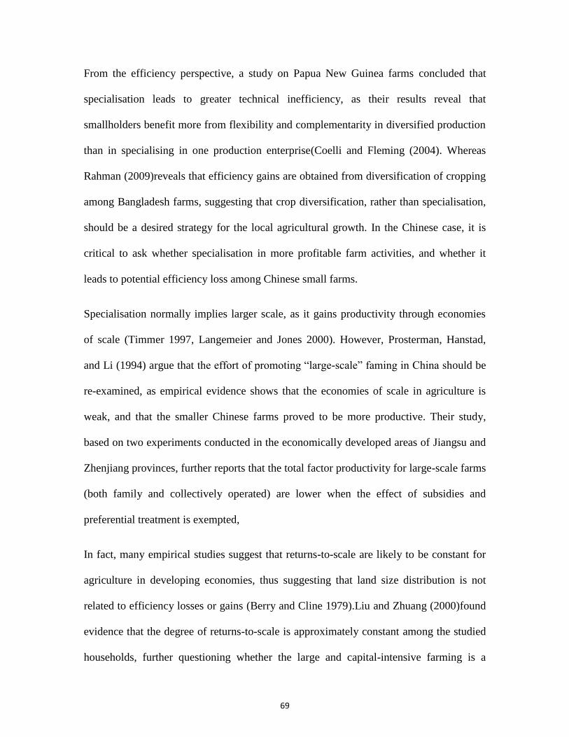
69
From the efficiency perspective, a study on Papua New Guinea farms concluded that
specialisation leads to greater technical inefficiency, as their results reveal that
smallholders benefit more from flexibility and complementarity in diversified production
than in specialising in one production enterprise(Coelli and Fleming (2004). Whereas
Rahman (2009)reveals that efficiency gains are obtained from diversification of cropping
among Bangladesh farms, suggesting that crop diversification, rather than specialisation,
should be a desired strategy for the local agricultural growth. In the Chinese case, it is
critical to ask whether specialisation in more profitable farm activities, and whether it
leads to potential efficiency loss among Chinese small farms.
Specialisation normally implies larger scale, as it gains productivity through economies
of scale (Timmer 1997, Langemeier and Jones 2000). However, Prosterman, Hanstad,
and Li (1994) argue that the effort of promoting “large-scale” faming in China should be
re-examined, as empirical evidence shows that the economies of scale in agriculture is
weak, and that the smaller Chinese farms proved to be more productive. Their study,
based on two experiments conducted in the economically developed areas of Jiangsu and
Zhenjiang provinces, further reports that the total factor productivity for large-scale farms
(both family and collectively operated) are lower when the effect of subsidies and
preferential treatment is exempted,
In fact, many empirical studies suggest that returns-to-scale are likely to be constant for
agriculture in developing economies, thus suggesting that land size distribution is not
related to efficiency losses or gains (Berry and Cline 1979).Liu and Zhuang (2000)found
evidence that the degree of returns-to-scale is approximately constant among the studied
households, further questioning whether the large and capital-intensive farming is a
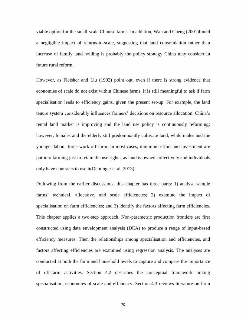
70
viable option for the small-scale Chinese farms. In addition, Wan and Cheng (2001)found
a negligible impact of returns-to-scale, suggesting that land consolidation rather than
increase of family land-holding is probably the policy strategy China may consider in
future rural reform.
However, as Fleisher and Liu (1992) point out, even if there is strong evidence that
economies of scale do not exist within Chinese farms, it is still meaningful to ask if farm
specialisation leads to efficiency gains, given the present set-up. For example, the land
tenure system considerably influences farmers’ decisions on resource allocation. China’s
rental land market is improving and the land use policy is continuously reforming;
however, females and the elderly still predominantly cultivate land, while males and the
younger labour force work off-farm. In most cases, minimum effort and investment are
put into farming just to retain the use rights, as land is owned collectively and individuals
only have contracts to use it(Deininger et al. 2013).
Following from the earlier discussions, this chapter has three parts: 1) analyse sample
farms’ technical, allocative, and scale efficiencies; 2) examine the impact of
specialisation on farm efficiencies; and 3) identify the factors affecting farm efficiencies.
This chapter applies a two-step approach. Non-parametric production frontiers are first
constructed using data envelopment analysis (DEA) to produce a range of input-based
efficiency measures. Then the relationships among specialisation and efficiencies, and
factors affecting efficiencies are examined using regression analysis. The analyses are
conducted at both the farm and household levels to capture and compare the importance
of off-farm activities. Section 4.2 describes the conceptual framework linking
specialisation, economies of scale and efficiency. Section 4.3 reviews literature on farm
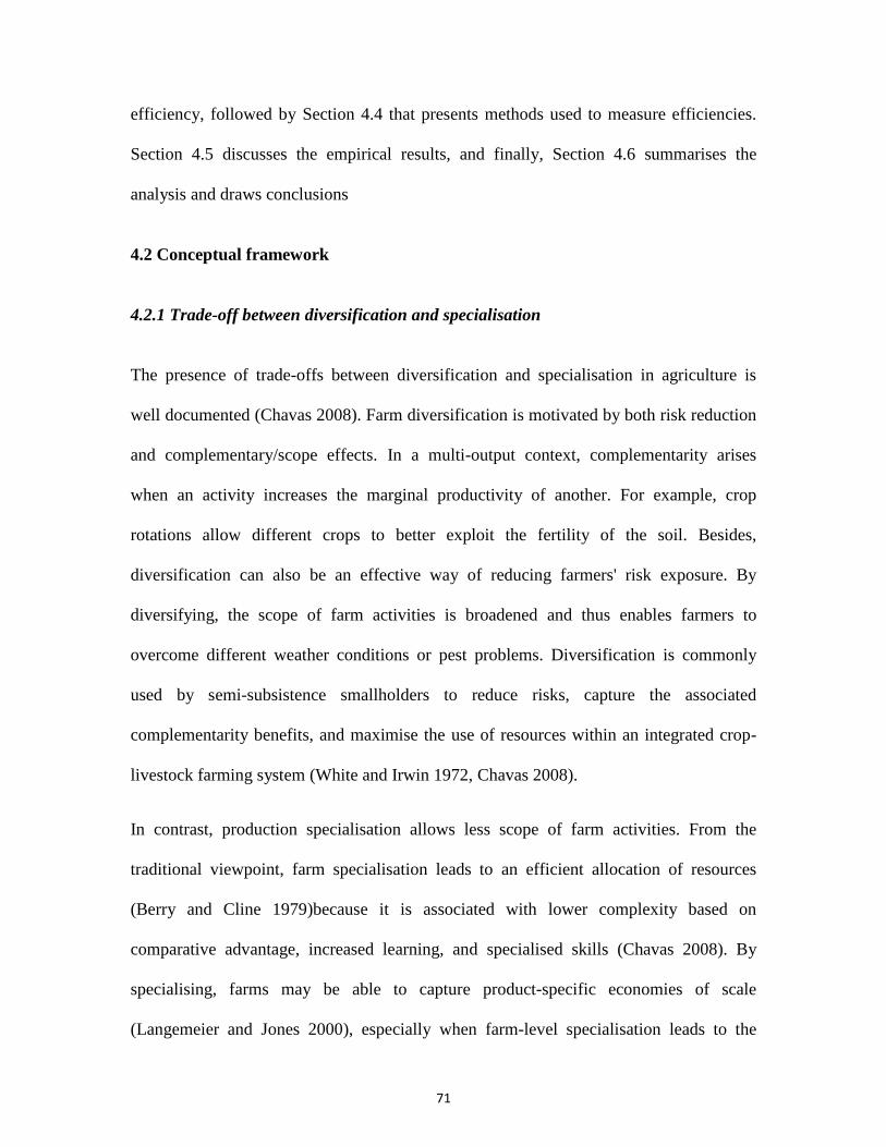
71
efficiency, followed by Section 4.4 that presents methods used to measure efficiencies.
Section 4.5 discusses the empirical results, and finally, Section 4.6 summarises the
analysis and draws conclusions
4.2 Conceptual framework
4.2.1 Trade-off between diversification and specialisation
The presence of trade-offs between diversification and specialisation in agriculture is
well documented (Chavas 2008). Farm diversification is motivated by both risk reduction
and complementary/scope effects. In a multi-output context, complementarity arises
when an activity increases the marginal productivity of another. For example, crop
rotations allow different crops to better exploit the fertility of the soil. Besides,
diversification can also be an effective way of reducing farmers' risk exposure. By
diversifying, the scope of farm activities is broadened and thus enables farmers to
overcome different weather conditions or pest problems. Diversification is commonly
used by semi-subsistence smallholders to reduce risks, capture the associated
complementarity benefits, and maximise the use of resources within an integrated crop-
livestock farming system (White and Irwin 1972, Chavas 2008).
In contrast, production specialisation allows less scope of farm activities. From the
traditional viewpoint, farm specialisation leads to an efficient allocation of resources
(Berry and Cline 1979)because it is associated with lower complexity based on
comparative advantage, increased learning, and specialised skills (Chavas 2008). By
specialising, farms may be able to capture product-specific economies of scale
(Langemeier and Jones 2000), especially when farm-level specialisation leads to the

72
adoption of new technologies. Often, it is associated with efficiency and productivity
increases (Lipton and Longhurst 1989), but in the process may also reduce famers’ ability
to manage risk (Langemeier and Jones 2000). The optimum degree of specialisation is to
a large extent dependent on the technical relationships between inputs and outputs for
each farm product(Heady 1952), being the reason why the efficiency and productivity
benefits are identified as an explanation of the historical trend toward more specialised
farms (Chavas 2008).
4.2.2 Specialisation, efficiency, and economies of scale – definitions and correlations
In economic theory, the concepts of efficiency, economies of scale (returns-to-scale), and
specialisation are closely related. Efficiency measures the performance of farms, and it is
usually used interchangeably with the term “productivity”9. In specific efficiency studies,
however, the concept of efficiency is more definite and strict, and is referred to as
economic efficiency. Economic efficiency measures the overall efficiency of technical
efficiency and allocative efficiency. A farm is technically efficient if it produces the
maximum output for a given amount of inputs, given the production technology available
to it. Allocative efficiency measures the extent to which the farm applies its inputs in the
optimal mix of outputs, taking input prices into consideration(Coelli and Rao 2005).
The effort of specialisation is usually explained by economies of scale and learning by
doing, excluding comparative advantage10. From a broad view, economies of scale refer
to the situation in which costs per unit of output fall as output increases(Colander,2013).
9According to Coelli et al. ( 2005), productivity is defined as the ratio of the output(s) that a farm produces
to the input(s) that it uses: productivity= outputs/inputs. 10Learning by doing can be simply described as becoming better at a task the more often a farmer performs
it (Colander, 2013).
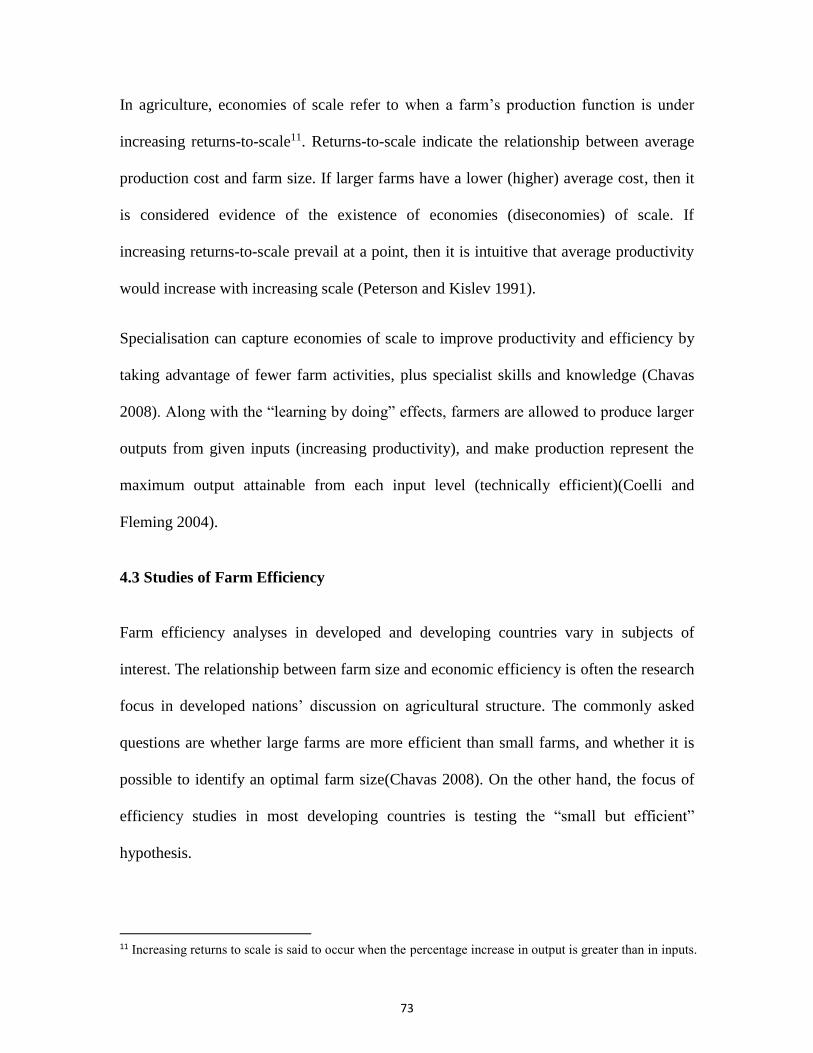
73
In agriculture, economies of scale refer to when a farm’s production function is under
increasing returns-to-scale11. Returns-to-scale indicate the relationship between average
production cost and farm size. If larger farms have a lower (higher) average cost, then it
is considered evidence of the existence of economies (diseconomies) of scale. If
increasing returns-to-scale prevail at a point, then it is intuitive that average productivity
would increase with increasing scale (Peterson and Kislev 1991).
Specialisation can capture economies of scale to improve productivity and efficiency by
taking advantage of fewer farm activities, plus specialist skills and knowledge (Chavas
2008). Along with the “learning by doing” effects, farmers are allowed to produce larger
outputs from given inputs (increasing productivity), and make production represent the
maximum output attainable from each input level (technically efficient)(Coelli and
Fleming 2004).
4.3 Studies of Farm Efficiency
Farm efficiency analyses in developed and developing countries vary in subjects of
interest. The relationship between farm size and economic efficiency is often the research
focus in developed nations’ discussion on agricultural structure. The commonly asked
questions are whether large farms are more efficient than small farms, and whether it is
possible to identify an optimal farm size(Chavas 2008). On the other hand, the focus of
efficiency studies in most developing countries is testing the “small but efficient”
hypothesis.
11 Increasing returns to scale is said to occur when the percentage increase in output is greater than in inputs.

74
4.3.1 Are larger farms more efficient? -- The relationship between farm size and
efficiency in developed countries
Farm size is a major concern in developed countries’ agriculture(Hansson 2008). The
past decades saw rapid structural changes with labour continuously leaving the
agricultural sector, farm enterprises increasing in size, and increasing concentration of
highly specialised farm businesses(OECD 2001). The fundamental reasons for the
structural changes are to increase productivity and farm return (land, labour and capital)
by either realising increasing returns to scale or by attaining larger production
volumes(Hansson 2008). However, the changing structure potentially affects the equity
within the agricultural sector, farm productivity and efficiency, and the demand for
government services and infrastructures (Tweeten 1984). A larger body of research
attempted to monitor this process and tried to understand the economic performance of
farms, in order for policies to be more responsive to the changing structure of agriculture.
In agricultural economics literature, the evidence of significant size-effects is used to
explain the decreasing number of small farms in developed economies. Large farms are
considered to be more economically efficient, as they are able to reduce their costs by
spreading fixed machinery and labour costs over more land and output, thus capturing
economies of scale (Hall and LeVeen 1978).However, empirical studies show mixed
results regarding this issue. For example, Aly et al. (1987) declared that larger farms were
more technically efficient than smaller farms, while Byrnes et al. (1987)found that their
sampled smaller farms are more technically efficient than larger farms. In addition, the
study by Garcia, Offutt, and Sonka (1987)shows that small farms were as economically
efficient as larger farms.
75
From the specialisation perspectives, Bagi (1982) reports that average technical
efficiency is higher for specialised crop farms than for mixed crop and livestock farms in
Tennessee (USA). Likewise, Heston and Sicular (2008) explore how efficiencies in
specialised Swedish dairy farms are affected by differences in farm size. The relationship
between farm size and efficiency is found to be non-linear in their study. While results
from Kansas (USA) farms indicate that technical efficiency varies by farm size, their
specialisation has no impact on productive efficiency (Mugera and Langemeier 2011).
The study on farms in Poland reveals that specialising in livestock production can lead to
technical and scale efficiencies, unlike the outcomes for crop farms (Latruffe et al. 2005)
Apparently, research results are contradictory with regard to the relationship between
farm size and economic efficiency. Kalaitzandonakes, Wu, and Ma (1992)argued that the
mixed empirical results could be partly due to the estimation procedures employed. It is
also proposed that this contradiction can be explained by the fact that the average cost
function in Western agriculture is L-shaped, meaning that the average cost declines as
farms are small to medium, but then plateaus as the farm becomes larger (Gorton and
Davidova 2004, Chavas 2008).
4.3.2 Small but efficient – subsistence farms in developing countries
A major rationale for examining efficiency in developing countries’ agriculture has been
to test the “small but efficient” hypothesis. Schultz’s (1964)work found that smallholder
farmers allocate their resources efficiently and rationally, as they rely heavily on their
own resources and have been attuned to their environment for many years. This
observation stimulates a large number of studies that test the efficiency of small farmers

76
in terms of technology application and resource allocation.
Empirical studies, however, demonstrate a substantial efficiency differential among small
farmers (Kalirajan 1981, Kalirajan 1990, Kalirajan and Shand 1985, Taylor and Wyatt
1996, Ali and Chaudhry 1990, Bravo-Ureta and Evenson 1994, Bagi 1982). The results
from those studies suggest that traditional agriculture is actually not economically
rational, nor price responsive. The significant efficiency differential among small farmers
motivated researchers to carry out research that enables them to identify factors that lead
some farmer to produce more than others with a given technology, inputs, and output
prices.
The earliest study to explore the determinants of efficiency is that of Shapiro and Müller
(1977). Their study found that technical efficiency has a high positive association with
general modernisation. Belbase and Grabowski (1985)pointed out that efficiency gains
could be obtained by getting extension and education. The adoption of new technologies
plays a key role in improving productivity in Nepalese agriculture.
Following the above pioneering work, a number of similar studies examined the
connection between efficiency and socioeconomic factors (income, education, experience,
extension), but the results were inconsistent. The majority of these studies found
education, experience, extension, and off-farm income are positively related to farm
efficiency (Kalirajan and Shand 1985, Bagi 1982, Kalirajan 1984, Kalirajan and Flinn
1983, Phillips and Marble 1986),however, Bravo-Ureta and Evenson (1994)found only a
weak correlation between efficiency and socioeconomic characteristics.
4.3.3 Previous efficiency studies of China
77
Most previous efficiency analyses undertaken in China focused on the macro-level,
especially in the efficiency improvement that resulted from institutional changes (i.e.
introduction of system and market liberalisation). For example, Fan (2000)reports that
technical efficiency increased by8.5% annually, while allocative efficiency had no
improvement (more than 87% of labour was overused) during China’s first phase of rural
reforms (1979-84) that focused on the decentralisation of the production system. The
second phase of reform (1985-93) focused on rural market liberalisation, and a slight
allocative and technical efficiency increase was achieved. This particular research also
points out the existence of regional variation in efficiency. A more detailed study by Jin,
Huang, and Rozelle (2010), that estimated the rate of changes in TFP for China’s main
farm commodities, concludes that China’s TFP growth rate was the world’s fastest
between 1978 and 2004. They attributed this to the development of technologies during
the same period.
At the provincial level, Mao and Koo (1997) estimated changes of technology and
efficiency in Chinese agricultural production for 29 provinces between 1984 and 1993.
The results show that farmers in coastal areas benefited from the rapid economic growth
and fewer market distortions, and obtained relatively high technical efficiency by
accessing new technology and market information. Chen, Huffman, and Rozelle
(2009)conducted a study on a large number of Chinese counties’ technical efficiency, and
found that cash crop production improves technical efficiency.
A few other micro-level studies investigated farm efficiency from various perspectives.
For example, Wang, Wailes, and Cramer (1996) examined the cause of inefficiency
among Chinese farm households. The study shows that both technical and allocative
78
efficiencies are restricted by market distortions and the absence of land use rights. Zhang
et al. (2011) explored the impact of land reallocation on technical efficiency for rural
households. Their results indicate that land reallocation affects technical efficiency
differently for farmers in different institutional and economic settings. Xu and Jeffrey
(1998)estimated the technical, allocative and economic efficiency of Chinese
conventional rice and hybrid rice producers in Jiangsu province. The results reveal
significant differences in technical and allocative efficiency between conventional and
hybrid rice production. Examining the effects of land rental market participation and off-
farm employment on technical efficiency, Feng (2008)reports that surveyed households
that rented land achieved higher technical efficiency, and further reported that the mean
technical efficiency is not affected by off-farm employment.
4.4 Methods
4.4.1 Production efficiency: concept and measurement
There are two approaches to efficiency analysis: Farrell (1957) established the frontier
approach, using the isoquant curve to measure economic efficiency. On the other
hand,Lau and Yotopoulos (1971) developed a dual profit function model to measure both
allocative and technical efficiency. Farrell’s frontier model is often applied in both
methodological and empirical studies due to its ability to provide farm-specific efficiency
measures, and it is consistent with the notion of maximum production, profit, and costs.
This method has been further developed into two major groups: non-parametric
production frontiers, and stochastic production frontiers(Bravo-Ureta and Pinheiro 1993).
Data Envelopment Analysis (DEA) is a non-parametric frontier analysis. It has been
79
demonstrated to be an effective method for measuring the relative efficiency of a set of
farms that utilise the same types of inputs to produce the same types of outputs. DEA
uses linear programming techniques to construct a piece-wise linear frontier that
“envelopes” the observed input and output data. It estimates the efficiency of the farm by
comparing its performance with the best practice farms chosen from its peers, and the
efficient frontier represents the sample farms’ production technology. Therefore, the
scores obtained are only relative to the best farm in the sample, and the mean efficiency
scores from different studies reflect only the dispersion of efficiencies within each sample,
and are not indicative of the efficiency level of one sample relative to another (Coelli and
Rao 2005).
4.4.1.1 Technical, allocative and cost efficiency
Conceptually, technical efficiency (TE) measures the degree of maximum feasible
output a farm can produce with its given amount of inputs, or the minimum feasible
inputs that can be used to produce a given level of output. Allocative efficiency (AE)
measures whether a technically efficient farm uses the optimal mix of inputs, given
the input prices; in other words, allocatively efficient farms minimise the production
costs. Cost efficiency (CE) is defined as the ratio of minimum (optimum) cost to the
observed cost for producing a given level of output by a farm. A measure of output
produced leads to the output-oriented efficiency analysis, while the input measure
approaches the input-oriented efficiency (Coelli and Rao 2005).
Figure 4.1 illustrates the concept of input-oriented measures of efficiency of a farm.
Assume that only two inputs 1x and 2x are used to produce a single output q, under the
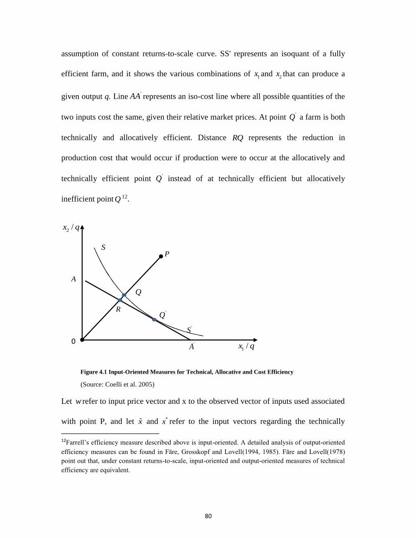
80
assumption of constant returns-to-scale curve. SS' represents an isoquant of a fully
efficient farm, and it shows the various combinations of 1x and 2x that can produce a
given output q. Line'AA represents an iso-cost line where all possible quantities of the
two inputs cost the same, given their relative market prices. At point 'Q a farm is both
technically and allocatively efficient. Distance RQ represents the reduction in
production cost that would occur if production were to occur at the allocatively and
technically efficient point 'Q instead of at technically efficient but allocatively
inefficient point Q 12.
Figure 4.1 Input-Oriented Measures for Technical, Allocative and Cost Efficiency
(Source: Coelli et al. 2005)
Let w refer to input price vector and x to the observed vector of inputs used associated
with point P, and let x̂ and *x refer to the input vectors regarding the technically
12Farrell’s efficiency measure described above is input-oriented. A detailed analysis of output-oriented
efficiency measures can be found in Färe, Grosskopf and Lovell(1994, 1985). Färe and Lovell(1978)
point out that, under constant returns-to-scale, input-oriented and output-oriented measures of technical
efficiency are equivalent.
2 /x q
1 /x q
A
0
S P
Q
'Q
'S
'A
R
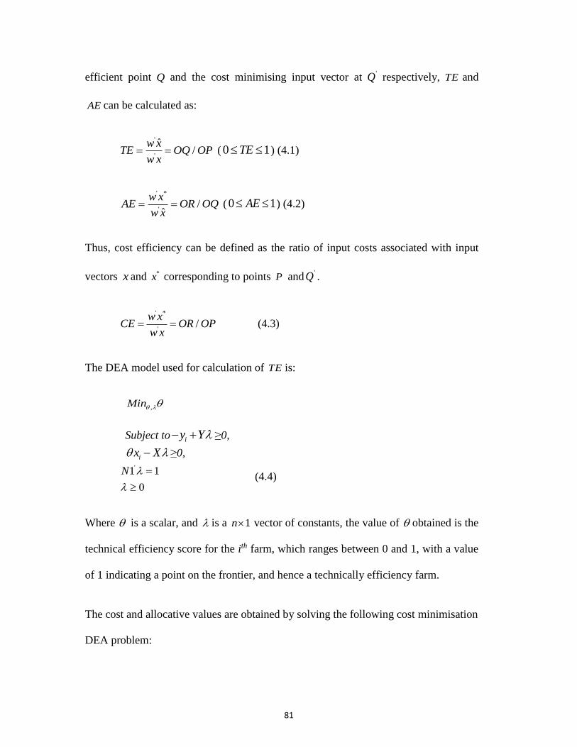
81
efficient point Q and the cost minimising input vector at 'Q respectively, TE and
AE can be calculated as:
'
'
ˆ/
w xTE OQ OP
w x ( 0 1TE ) (4.1)
' *
'/
ˆ
w xAE OR OQ
w x ( 0 1AE ) (4.2)
Thus, cost efficiency can be defined as the ratio of input costs associated with input
vectors x and *x corresponding to points P and'Q .
' *
'/
w xCE OR OP
w x (4.3)
The DEA model used for calculation of TE is:
,Min
Subject to iy Y ≥0,
ix X ≥0,
'1 1
0
N
(4.4)
Where is a scalar, and is a 1n vector of constants, the value of obtained is the
technical efficiency score for the ith farm, which ranges between 0 and 1, with a value
of 1 indicating a point on the frontier, and hence a technically efficiency farm.
The cost and allocative values are obtained by solving the following cost minimisation
DEA problem:
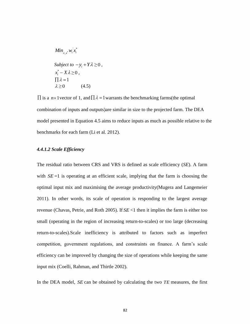
82
*
' *
, i ixMin w x
Subject to iy Y ≥ 0 ,
*
ix X ≥ 0 ,
1
≥0 (4.5)
is a 1n vector of 1, and 1 warrants the benchmarking farms(the optimal
combination of inputs and outputs)are similar in size to the projected farm. The DEA
model presented in Equation 4.5 aims to reduce inputs as much as possible relative to the
benchmarks for each farm (Li et al. 2012).
4.4.1.2 Scale Efficiency
The residual ratio between CRS and VRS is defined as scale efficiency (SE). A farm
with SE =1 is operating at an efficient scale, implying that the farm is choosing the
optimal input mix and maximising the average productivity(Mugera and Langemeier
2011). In other words, its scale of operation is responding to the largest average
revenue (Chavas, Petrie, and Roth 2005). If SE <1 then it implies the farm is either too
small (operating in the region of increasing return-to-scales) or too large (decreasing
return-to-scales).Scale inefficiency is attributed to factors such as imperfect
competition, government regulations, and constraints on finance. A farm’s scale
efficiency can be improved by changing the size of operations while keeping the same
input mix (Coelli, Rahman, and Thirtle 2002).
In the DEA model, SE can be obtained by calculating the two TE measures, the first
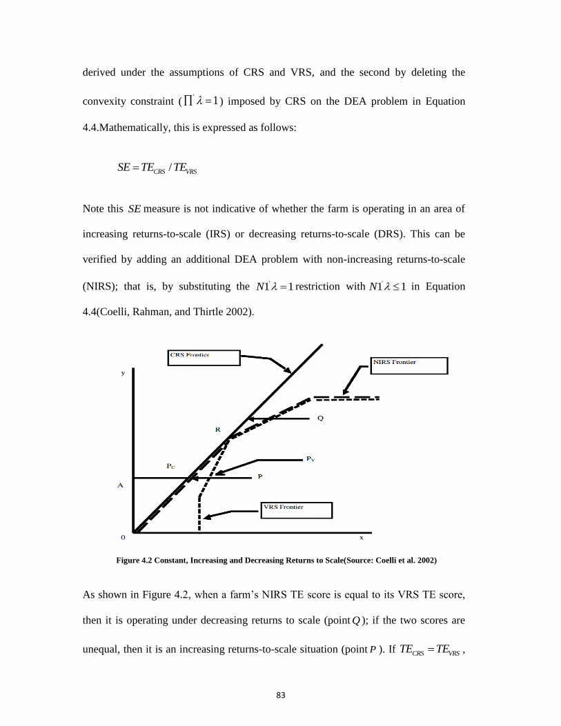
83
derived under the assumptions of CRS and VRS, and the second by deleting the
convexity constraint (' 1 ) imposed by CRS on the DEA problem in Equation
4.4.Mathematically, this is expressed as follows:
/CRS VRSSE TE TE
Note this SE measure is not indicative of whether the farm is operating in an area of
increasing returns-to-scale (IRS) or decreasing returns-to-scale (DRS). This can be
verified by adding an additional DEA problem with non-increasing returns-to-scale
(NIRS); that is, by substituting the '1 1N restriction with '1 1N in Equation
4.4(Coelli, Rahman, and Thirtle 2002).
Figure 4.2 Constant, Increasing and Decreasing Returns to Scale(Source: Coelli et al. 2002)
As shown in Figure 4.2, when a farm’s NIRS TE score is equal to its VRS TE score,
then it is operating under decreasing returns to scale (point Q ); if the two scores are
unequal, then it is an increasing returns-to-scale situation (point P ). If CRS VRSTE TE ,
84
it implies constant return- to-scale. In microeconomics theory, CRS indicates a farm’s
operation is at its most productive plant size with cost minimisation and revenue
maximised. In the short run, farms may operate in either the IRS or DRS zones, but
will more likely move towards CRS by scaling up or scaling down their size in the
long run (Kumar and Gulati 2008).
4.4.1.3 Data requirements
Aggregation of variables has been a concern in the literature regarding efficiency analysis.
A trade-off exists between the loss of degrees of freedom and the inclusion of a large
number of input and output categories (Coelli and Fleming 2004). Although some argue
that aggregation of inputs or outputs should be avoided, if possible (Preckel, Akridge, and
Boland 1997),others show that a proper number of inputs and outputs relative to sample
size is expected to produce a practical number of “efficient” production units (Chavas,
Petrie, and Roth 2005). According to Fernandez-Cornejo (1993), if the number of
observations divided by the sum of the number of inputs and outputs is larger than five,
then the dimensionality ratio is sufficient to differentiate efficiency variance in a given
sample of farms.
In this study, surveyed farmer produced large range of crops and a variety of livestock;
therefore, multitude types of inputs were applied. To avoid the “over-efficient bias”
mentioned earlier, various outputs were aggregated into crop and livestock production,
and some of the inputs such as fertilisers and labour were also aggregated into different
categories13.Eventually, the aggregation process ends up with two output and six input
13In total, eleven crops and five types of animals were used for total farm output formulation; these were
wheat, maize, beans, potato, rapeseed, fruit, vegetables, melons, seedlings, forage, and apple.livestock.
85
categorise that were used to estimate 317 sample farms’ efficiency frontiers. Input data
used for the efficiency analysis include: (a) cultivated land, including rented land (Mu);
(b) labour, both family and hired in man-days; (c)fertilisers 14 (kg); (d) seed (kg);
(e)machinery input (measured by machine operated land area, Mu); (f) feedstuff (kg).
Farm outputs used in the estimation include crop and livestock, measured by production
value (Yuan). The choice of input and output aggregates appears reasonable for the
purpose of this research model. However, different commodity aggregations could
influence the efficiency scores estimated (Coelli et al. 2005).
Estimation of the allocative and cost efficiency requires data on prices. In order to
capture price deviations among farms, considerable effort was made in this study to
collect prices of each commodity from individual households. Price information at local
markets was also gathered for the reference of average prices. Reasonable price
variations were observed across farms, as a result of seasonal effects (purchased and/or
sold at different points during the year) and differential access to markets, which is
considered as an indication of market imperfection and the transaction cost differential
facing farmers (Chavas and Aliber 1993).Price data for aggregated inputs followed the
“unit value” method suggested by Coelli et al. (2005). For example, the price for input
“fertilisers” was derived from averaging the price for fourteen different fertilisers. The
hired labour price was used as an opportunity cost for family farm labour. The price for
self-grown forage/feedstuff was substituted by corresponding market price. Quantity data
for machinery input was unavailable so a proxy variable was used. Prices for hiring
included: draft animals, sheep/goats, cattle, poultry, pigs. 14The fourteen categories of fertilisers used among farms for different cropsare: 1 Ammonium bicarbonate;
2 Urea; 3 DAP; 4 Mixed fertiliser; 5 Superphosphate; 6 Potash; 7 Ammonium; 8 Nitrate Cyanamid; 9
Ammonium; 10 Ammonia; 11 Corn special; 12 Soybean special; 13 Phosphate; 14 Zinc.
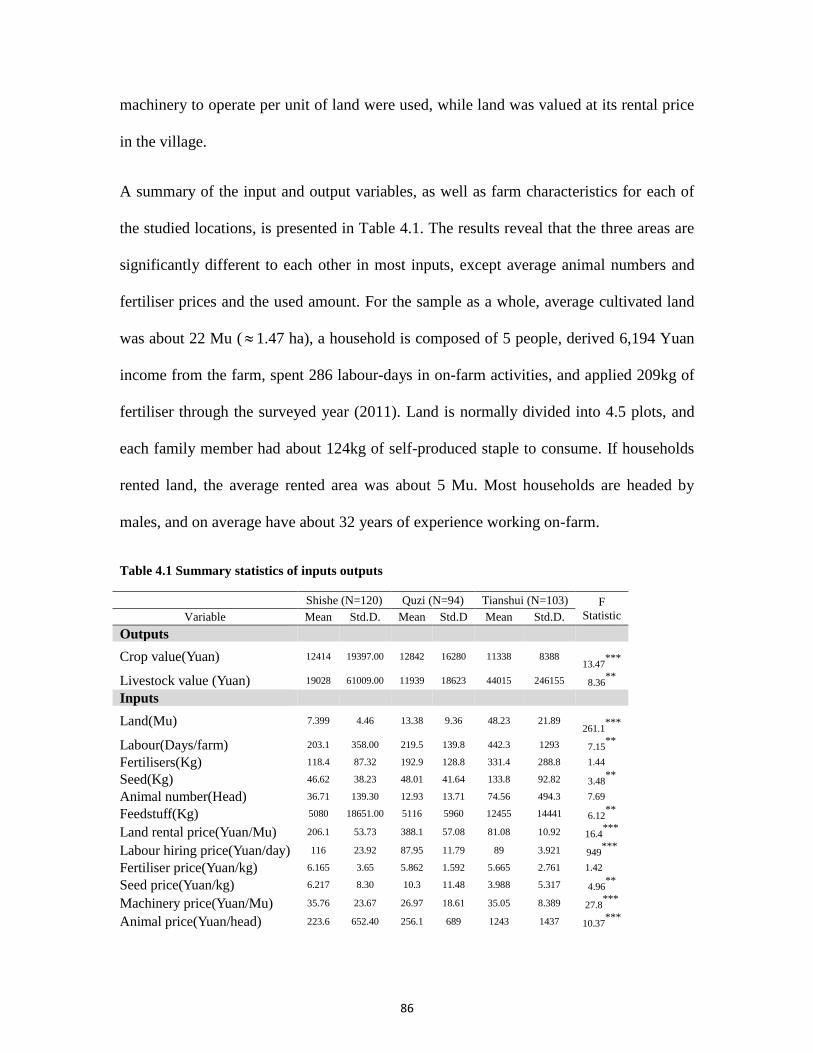
86
machinery to operate per unit of land were used, while land was valued at its rental price
in the village.
A summary of the input and output variables, as well as farm characteristics for each of
the studied locations, is presented in Table 4.1. The results reveal that the three areas are
significantly different to each other in most inputs, except average animal numbers and
fertiliser prices and the used amount. For the sample as a whole, average cultivated land
was about 22 Mu ( 1.47 ha), a household is composed of 5 people, derived 6,194 Yuan
income from the farm, spent 286 labour-days in on-farm activities, and applied 209kg of
fertiliser through the surveyed year (2011). Land is normally divided into 4.5 plots, and
each family member had about 124kg of self-produced staple to consume. If households
rented land, the average rented area was about 5 Mu. Most households are headed by
males, and on average have about 32 years of experience working on-farm.
Table 4.1 Summary statistics of inputs outputs
Shishe (N=120) Quzi (N=94) Tianshui (N=103) F
Statistic Variable Mean Std.D. Mean Std.D Mean Std.D.
Outputs
Crop value(Yuan) 12414 19397.00 12842 16280 11338 8388
13.47***
Livestock value (Yuan) 19028 61009.00 11939 18623 44015 246155 8.36**
Inputs
Land(Mu) 7.399 4.46 13.38 9.36 48.23 21.89
261.1***
Labour(Days/farm) 203.1 358.00 219.5 139.8 442.3 1293 7.15**
Fertilisers(Kg) 118.4 87.32 192.9 128.8 331.4 288.8 1.44
Seed(Kg) 46.62 38.23 48.01 41.64 133.8 92.82 3.48**
Animal number(Head) 36.71 139.30 12.93 13.71 74.56 494.3 7.69
Feedstuff(Kg) 5080 18651.00 5116 5960 12455 14441 6.12**
Land rental price(Yuan/Mu) 206.1 53.73 388.1 57.08 81.08 10.92 16.4***
Labour hiring price(Yuan/day) 116 23.92 87.95 11.79 89 3.921 949***
Fertiliser price(Yuan/kg) 6.165 3.65 5.862 1.592 5.665 2.761 1.42
Seed price(Yuan/kg) 6.217 8.30 10.3 11.48 3.988 5.317 4.96**
Machinery price(Yuan/Mu) 35.76 23.67 26.97 18.61 35.05 8.389 27.8***
Animal price(Yuan/head) 223.6 652.40 256.1 689 1243 1437 10.37***

87
**p< 0.01, ***p< 0.001
4.4.2 Impacts of specialisation on efficiency
Once the efficiency measures of TE, AE, CE, and SE are obtained from the DEA, the
impact of specialisation on efficiency and the determinants of inefficiency was
investigated by econometric modelling. Tobit estimation in the second stage DEA
efficiency analyses is most commonly used to identify factors influencing efficiency in
various studies (Wu and Prato 2006, Chavas 2001, Coelli, Rahman, and Thirtle 2002,
Hansson 2008, Haji 2007) Compared to the stochastic production frontier (SPF), DEA is
a non-parametric method that no assumptions are required either for relationship between
inputs and outputs, nor the distribution of efficiency scores. Because DEA is able to
accommodate endogenous variables, and variables that are categorical and/or
classificatory(Coelli et al., 1999 ). Therefore, Tobit regression is the most-often used
approach to modelling the DEA scores against exogenous variables, and is proved to be
sufficient in most cases compared to OLS linear regression ( Hoff, 2006)
4.4.2.1 The Tobit model
The Tobit regression model is specified as:
*
i j j
j
E x v
1iE if * 1iE
*
i iE E if*
iE <1
Feedstuff price(Yuan/kg) 2.235 0.61 2.006 0.244 1.997 0.337 12.9**
88
Where iE is an efficiency score, x is a vector of explanatory variables,
2(0, )v N andj are the parameters of interest (Tobin 1958).
4.4.2.2 Variables
Explanatory variables in the Tobit model reflect factors that affect decision-making and
control of resources within the household, or proxies for factor market endowments and
institutions that affect access to and utilisation of land, labour and financial capital. Those
variables include: specialisation, output value (indicator of farm size15), family size,
capital assets, and agro-equipment, land plots, hired labour, share of off-farm income and
location dummies. Other variables, such as highest education level attained by the
household head, head gender, and farming experience, have been traditionally used in the
literature to explain variations in efficiency (Chavas, Petrie, and Roth 2005). The second
section of Table 4.1 presents the summary statistics of the farm-specific variables.
As noted earlier, the purpose of the econometric analysis is to investigate how
specialisation affects farm efficiency. The dependent variable in our econometrics is the
specialisation index. Both farm specialisation and household specialisation Tobit models
were used in this study. At the household level, off-farm activities were considered. As
stressed in Section 2.3, it is necessary to include off-farm activities in farm household
efficiency analysis, as off-farm income could stimulate farm investments and
productivity, and an imperfect labour market can contribute to inefficiency of labour
allocation (Chavas, Petrie, and Roth 2005).
15 As a variable of farm operation scale, farm size can be measured by either land area, value added, output
value, output volume, or labour input (Eastwood, Lipton, and Newell 2010)
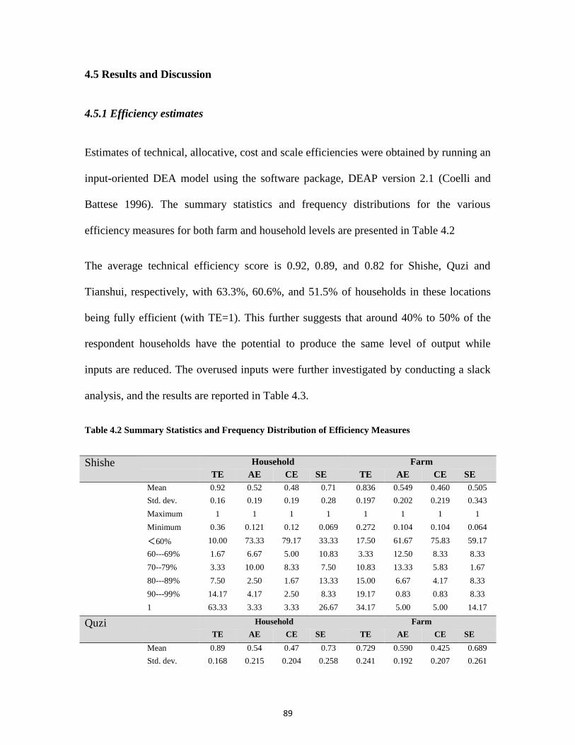
89
4.5 Results and Discussion
4.5.1 Efficiency estimates
Estimates of technical, allocative, cost and scale efficiencies were obtained by running an
input-oriented DEA model using the software package, DEAP version 2.1 (Coelli and
Battese 1996). The summary statistics and frequency distributions for the various
efficiency measures for both farm and household levels are presented in Table 4.2
The average technical efficiency score is 0.92, 0.89, and 0.82 for Shishe, Quzi and
Tianshui, respectively, with 63.3%, 60.6%, and 51.5% of households in these locations
being fully efficient (with TE=1). This further suggests that around 40% to 50% of the
respondent households have the potential to produce the same level of output while
inputs are reduced. The overused inputs were further investigated by conducting a slack
analysis, and the results are reported in Table 4.3.
Table 4.2 Summary Statistics and Frequency Distribution of Efficiency Measures
Shishe
Household Farm
TE AE CE SE TE AE CE SE
Mean 0.92 0.52 0.48 0.71 0.836 0.549 0.460 0.505
Std. dev. 0.16 0.19 0.19 0.28 0.197 0.202 0.219 0.343
Maximum 1 1 1 1 1 1 1 1
Minimum 0.36 0.121 0.12 0.069 0.272 0.104 0.104 0.064
<60% 10.00 73.33 79.17 33.33 17.50 61.67 75.83 59.17
60---69% 1.67 6.67 5.00 10.83 3.33 12.50 8.33 8.33
70--79% 3.33 10.00 8.33 7.50 10.83 13.33 5.83 1.67
80---89% 7.50 2.50 1.67 13.33 15.00 6.67 4.17 8.33
90---99% 14.17 4.17 2.50 8.33 19.17 0.83 0.83 8.33
1 63.33 3.33 3.33 26.67 34.17 5.00 5.00 14.17
Quzi Household Farm
TE AE CE SE TE AE CE SE
Mean 0.89 0.54 0.47 0.73 0.729 0.590 0.425 0.689
Std. dev. 0.168 0.215 0.204 0.258 0.241 0.192 0.207 0.261
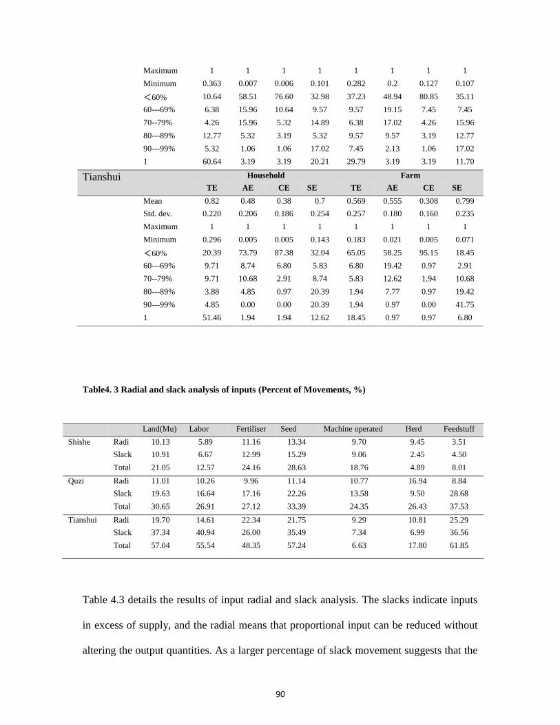
90
Maximum 1 1 1 1 1 1 1 1
Minimum 0.363 0.007 0.006 0.101 0.282 0.2 0.127 0.107
<60% 10.64 58.51 76.60 32.98 37.23 48.94 80.85 35.11
60---69% 6.38 15.96 10.64 9.57 9.57 19.15 7.45 7.45
70--79% 4.26 15.96 5.32 14.89 6.38 17.02 4.26 15.96
80---89% 12.77 5.32 3.19 5.32 9.57 9.57 3.19 12.77
90---99% 5.32 1.06 1.06 17.02 7.45 2.13 1.06 17.02
1 60.64 3.19 3.19 20.21 29.79 3.19 3.19 11.70
Tianshui Household Farm
TE AE CE SE TE AE CE SE
Mean 0.82 0.48 0.38 0.7 0.569 0.555 0.308 0.799
Std. dev. 0.220 0.206 0.186 0.254 0.257 0.180 0.160 0.235
Maximum 1 1 1 1 1 1 1 1
Minimum 0.296 0.005 0.005 0.143 0.183 0.021 0.005 0.071
<60% 20.39 73.79 87.38 32.04 65.05 58.25 95.15 18.45
60---69% 9.71 8.74 6.80 5.83 6.80 19.42 0.97 2.91
70--79% 9.71 10.68 2.91 8.74 5.83 12.62 1.94 10.68
80---89% 3.88 4.85 0.97 20.39 1.94 7.77 0.97 19.42
90---99% 4.85 0.00 0.00 20.39 1.94 0.97 0.00 41.75
1 51.46 1.94 1.94 12.62 18.45 0.97 0.97 6.80
Table4. 3 Radial and slack analysis of inputs (Percent of Movements, %)
Table 4.3 details the results of input radial and slack analysis. The slacks indicate inputs
in excess of supply, and the radial means that proportional input can be reduced without
altering the output quantities. As a larger percentage of slack movement suggests that the
Land(Mu)
( Mu)
Labor
(days)
Fertiliser
( kg)
Seed
(Kg)
Machine operated
area(Mu)
Herd
size
Feedstuff
(Kg) Shishe Radi
al
10.13 5.89 11.16 13.34 9.70 9.45 3.51
Slack 10.91 6.67 12.99 15.29 9.06 2.45 4.50
Total 21.05 12.57 24.16 28.63 18.76 4.89 8.01
Quzi Radi
al
11.01 10.26 9.96 11.14 10.77 16.94 8.84
Slack 19.63 16.64 17.16 22.26 13.58 9.50 28.68
Total 30.65 26.91 27.12 33.39 24.35 26.43 37.53
Tianshui Radi
al
19.70 14.61 22.34 21.75 9.29 10.81 25.29
Slack 37.34 40.94 26.00 35.49 7.34 6.99 36.56
Total 57.04 55.54 48.35 57.24 6.63 17.80 61.85
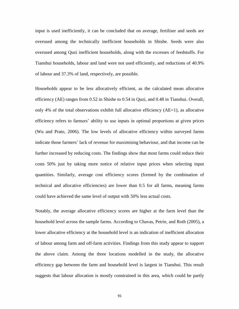
91
input is used inefficiently, it can be concluded that on average, fertiliser and seeds are
overused among the technically inefficient households in Shishe. Seeds were also
overused among Quzi inefficient households, along with the excesses of feedstuffs. For
Tianshui households, labour and land were not used efficiently, and reductions of 40.9%
of labour and 37.3% of land, respectively, are possible.
Households appear to be less allocatively efficient, as the calculated mean allocative
efficiency (AE) ranges from 0.52 in Shishe to 0.54 in Quzi, and 0.48 in Tianshui. Overall,
only 4% of the total observations exhibit full allocative efficiency (AE=1), as allocative
efficiency refers to farmers’ ability to use inputs in optimal proportions at given prices
(Wu and Prato, 2006). The low levels of allocative efficiency within surveyed farms
indicate those farmers’ lack of revenue for maximising behaviour, and that income can be
further increased by reducing costs. The findings show that most farms could reduce their
costs 50% just by taking more notice of relative input prices when selecting input
quantities. Similarly, average cost efficiency scores (formed by the combination of
technical and allocative efficiencies) are lower than 0.5 for all farms, meaning farms
could have achieved the same level of output with 50% less actual costs.
Notably, the average allocative efficiency scores are higher at the farm level than the
household level across the sample farms. According to Chavas, Petrie, and Roth (2005), a
lower allocative efficiency at the household level is an indication of inefficient allocation
of labour among farm and off-farm activities. Findings from this study appear to support
the above claim. Among the three locations modelled in the study, the allocative
efficiency gap between the farm and household level is largest in Tianshui. This result
suggests that labour allocation is mostly constrained in this area, which could be partly
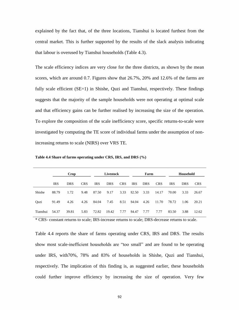
92
explained by the fact that, of the three locations, Tianshui is located furthest from the
central market. This is further supported by the results of the slack analysis indicating
that labour is overused by Tianshui households (Table 4.3).
The scale efficiency indices are very close for the three districts, as shown by the mean
scores, which are around 0.7. Figures show that 26.7%, 20% and 12.6% of the farms are
fully scale efficient (SE=1) in Shishe, Quzi and Tianshui, respectively. These findings
suggests that the majority of the sample households were not operating at optimal scale
and that efficiency gains can be further realised by increasing the size of the operation.
To explore the composition of the scale inefficiency score, specific returns-to-scale were
investigated by computing the TE score of individual farms under the assumption of non-
increasing returns to scale (NIRS) over VRS TE.
Table 4.4 Share of farms operating under CRS, IRS, and DRS (%)
Crop Livestock Farm Household
IRS DRS CRS IRS DRS CRS IRS DRS CRS IRS DRS CRS
Shishe 88.79 1.72 9.48 87.50 9.17 3.33 82.50 3.33 14.17 70.00 3.33 26.67
Quzi 91.49 4.26 4.26 84.04 7.45 8.51 84.04 4.26 11.70 78.72 1.06 20.21
Tianshui 54.37 39.81 5.83 72.82 19.42 7.77 84.47 7.77 7.77 83.50 3.88 12.62
* CRS- constant returns to scale; IRS-increase returns to scale; DRS-decrease returns to scale.
Table 4.4 reports the share of farms operating under CRS, IRS and DRS. The results
show most scale-inefficient households are “too small” and are found to be operating
under IRS, with70%, 78% and 83% of households in Shishe, Quzi and Tianshui,
respectively. The implication of this finding is, as suggested earlier, these households
could further improve efficiency by increasing the size of operation. Very few
93
households (less than 4%) are found to be too big and operating under DRS.
About 27% of farms in Shishe operated at CRS, indicating that these farmers were
operating at optimal scale in terms of land or/and labour. The percentages of farms under
CRS for Quzi and Tianshui are 20.2% and 12.6%, respectively. Among the scale-
inefficient households, the majority (about 80%) exhibit increasing returns-to-scale. This
is also true for the whole farm, crop and livestock production. The research findings that
the majority of Chinese farms are operating under increasing returns-to-scale is consistent
with the case study by Li et al.(2012),which investigated99 farms from China’s Hebei
province using the DEA approach. Other studies report that CRS prevails in Chinese
agriculture, when the returns-to-scale is measured using the Cobb-Douglas production
function model specification. In these studies, the sum of coefficients is found to be
greater than 1.0(Liu and Zhuang 2000, Fleisher and Liu 1992, Wan and Cheng 2001).
4.5.2 Factors explaining efficiencies
To ascertain the impact of specialisation on efficiency, a Tobit model specification was
employed. The analysis was conducted by pooling data across all three study locations.
The regression results are reported in Tables 4.5 to 4.8.
Overall, the results reveal that specialisation increases households’ technical efficiency
and cost efficiency, but has no effect on allocative and scale efficiency. This is also true
for the farm-level analyses. This result further suggests that when households focus on
fewer activities, either farm or off-farm in nature, they are more capable of minimising
input use in producing a given level of outputs. That is, they are able to achieve the same
level of output with less cost, compared with households with more diversified farm

94
and/or off-farm activities. These results confirm the hypothesis that the degree of
specialisation is related to the technical relationships between inputs and outputs(Heady
1952), and technical efficiency can be improved by skills specialisation and by the effects
of “learning by doing” (Coelli and Fleming 2004, Timmer 1997).
It is not a surprise that specialisation has no impact on allocative efficiency, as reducing
farm/household activities does not necessarily change the optimal level of input mix, with
a given input price. This is possible when resources are mobile and corresponding
technologies are available (Chavas 2001).In addition, specialisation is shown to be
independent of scale efficiency. This is as expected, as specialisation only reduces the
scope, but not the scale of farm/household production (Coelli et al. 2005).
In terms of other factors that influence efficiencies, items such as food subsistence,
migration, land fragmentation and farm size are shown to significantly affect farm/
household efficiencies. First, food subsistence, which indicates the ability of the
household to produce staple grains, is found to increase household and farm technical
efficiency. This outcome can be partly explained by the fact that food security can
increase household labour productivity through higher nutrition intake (Chavas, Petrie,
and Roth 2005).
Second, a significant relationship is revealed to exist between migration and household
efficiency (shown through Tables 4.5 to 4.8), further showing evidence that off-farm
activity negatively affects households’ technical efficiency, but positively influences
allocative efficiency, cost efficiency, and scale efficiency. This finding is consistent with
the hypothesis that smooth access to the labour market contributes to efficient resource

95
(especially labour) allocation. However, losing a productive labour force to migration
will indeed lead to decreasing technical efficiency.
Third, Table 4.7 shows that when households’ land is divided into more plots, it leads to
technical and cost inefficiency, but has no significant effect on allocative and scale
efficiency. This result is consistent with the theory that the adverse effects of land
fragmentation on technical and cost efficiencies exist because: a) plot boundaries and
access routes result in loss of land; b) travelling among plots costs extra labour and fuel
inputs; c) inputs such as fertiliser, water and pesticide could be wasted more as leakage
and evaporation increased with growing plot numbers and boundaries (Wan and Cheng
2001). The results reveal that land consolidation may be an effective way to improve
outputs and to save costs, but not necessarily help farms to expand their scale efficiency.
Finally, farm income, as a proxy of farm size, is found to be independent of technical,
allocative and cost efficiencies, but positively associated with scale efficiency, indicating
that larger farms are relatively operating at optimal size. A simple OLS analysis reveals
that a 1% increase in scale efficiency can increase farm income by about 28,118 Yuan. In
addition, Table 4.9 also indicates that specialised farms have even greater increases in
farm income than diversified farms, as indicated by the farm-type dummy variable in
both models in Table 4.9.
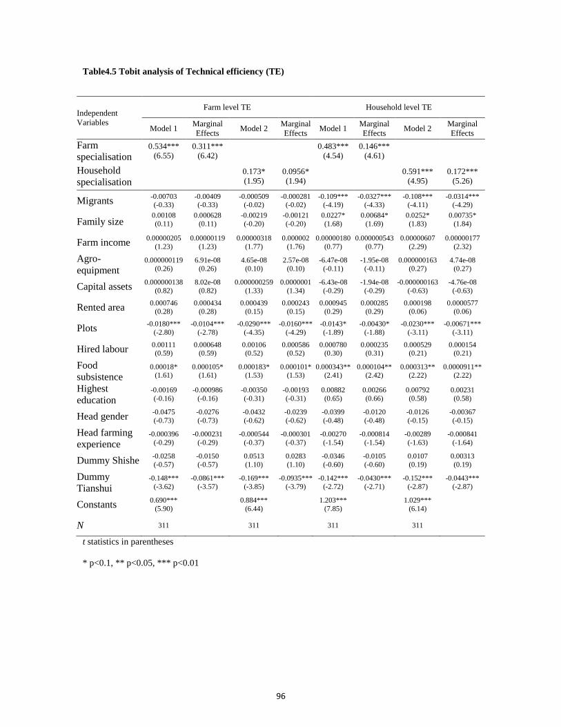
96
Table4.5 Tobit analysis of Technical efficiency (TE)
Independent
Variables
Farm level TE Household level TE
Model 1 Marginal
Effects Model 2
Marginal
Effects Model 1
Marginal
Effects Model 2
Marginal
Effects
Farm
specialisation 0.534***
(6.55)
0.311***
(6.42)
0.483***
(4.54)
0.146***
(4.61)
Household
specialisation
0.173*
(1.95)
0.0956*
(1.94)
0.591***
(4.95)
0.172***
(5.26)
Migrants -0.00703 (-0.33)
-0.00409 (-0.33)
-0.000509 (-0.02)
-0.000281 (-0.02)
-0.109*** (-4.19)
-0.0327*** (-4.33)
-0.108*** (-4.11)
-0.0314*** (-4.29)
Family size 0.00108
(0.11)
0.000628
(0.11)
-0.00219
(-0.20)
-0.00121
(-0.20)
0.0227*
(1.68)
0.00684*
(1.69)
0.0252*
(1.83)
0.00735*
(1.84)
Farm income 0.00000205
(1.23)
0.00000119
(1.23)
0.00000318
(1.77)
0.000002
(1.76)
0.00000180
(0.77)
0.000000543
(0.77)
0.00000607
(2.29)
0.00000177
(2.32)
Agro-
equipment 0.000000119
(0.26)
6.91e-08
(0.26)
4.65e-08
(0.10)
2.57e-08
(0.10)
-6.47e-08
(-0.11)
-1.95e-08
(-0.11)
0.000000163
(0.27)
4.74e-08
(0.27)
Capital assets 0.000000138
(0.82)
8.02e-08
(0.82)
0.000000259
(1.33)
0.0000001
(1.34)
-6.43e-08
(-0.29)
-1.94e-08
(-0.29)
-0.000000163
(-0.63)
-4.76e-08
(-0.63)
Rented area 0.000746
(0.28)
0.000434
(0.28)
0.000439
(0.15)
0.000243
(0.15)
0.000945
(0.29)
0.000285
(0.29)
0.000198
(0.06)
0.0000577
(0.06)
Plots -0.0180***
(-2.80)
-0.0104***
(-2.78)
-0.0290***
(-4.35)
-0.0160***
(-4.29)
-0.0143*
(-1.89)
-0.00430*
(-1.88)
-0.0230***
(-3.11)
-0.00671***
(-3.11)
Hired labour 0.00111 (0.59)
0.000648 (0.59)
0.00106 (0.52)
0.000586 (0.52)
0.000780 (0.30)
0.000235 (0.31)
0.000529 (0.21)
0.000154 (0.21)
Food
subsistence 0.00018*
(1.61) 0.000105*
(1.61) 0.000183*
(1.53) 0.000101*
(1.53) 0.000343**
(2.41) 0.000104**
(2.42) 0.000313**
(2.22) 0.0000911**
(2.22)
Highest
education -0.00169
(-0.16)
-0.000986
(-0.16)
-0.00350
(-0.31)
-0.00193
(-0.31)
0.00882
(0.65)
0.00266
(0.66)
0.00792
(0.58)
0.00231
(0.58)
Head gender -0.0475
(-0.73)
-0.0276
(-0.73)
-0.0432
(-0.62)
-0.0239
(-0.62)
-0.0399
(-0.48)
-0.0120
(-0.48)
-0.0126
(-0.15)
-0.00367
(-0.15)
Head farming
experience -0.000396
(-0.29)
-0.000231
(-0.29)
-0.000544
(-0.37)
-0.000301
(-0.37)
-0.00270
(-1.54)
-0.000814
(-1.54)
-0.00289
(-1.63)
-0.000841
(-1.64)
Dummy Shishe -0.0258
(-0.57)
-0.0150
(-0.57)
0.0513
(1.10)
0.0283
(1.10)
-0.0346
(-0.60)
-0.0105
(-0.60)
0.0107
(0.19)
0.00313
(0.19)
Dummy
Tianshui -0.148***
(-3.62)
-0.0861***
(-3.57)
-0.169***
(-3.85)
-0.0935***
(-3.79)
-0.142***
(-2.72)
-0.0430***
(-2.71)
-0.152***
(-2.87)
-0.0443***
(-2.87)
Constants 0.690***
(5.90)
0.884***
(6.44)
1.203***
(7.85)
1.029***
(6.14)
N 311 311 311 311
t statistics in parentheses
* p<0.1, ** p<0.05, *** p<0.01
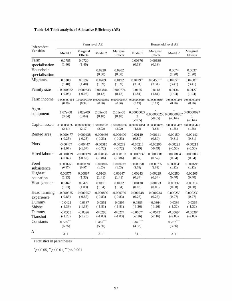
97
Table 4.6 Tobit analysis of Allocative Efficiency (AE)
Independent
Variables
Farm level AE Household level AE
Model 1 Marginal
Effects Model 2
Marginal
Effects Model 1
Marginal
Effects Model 2
Marginal
Effects
Farm
specialisation 0.0785
(1.40)
0.0720
(1.40)
0.00676
(0.13)
0.00639
(0.13)
Household
specialisation
0.0220
(0.38)
0.0202
(0.38)
0.0674
(1.20)
0.0637
(1.20)
Migrants 0.0209
(1.40)
0.0192
(1.40)
0.0209
(1.39)
0.0192
(1.39)
0.0479**
(3.31)
0.0453***
(3.31)
0.0495***
(3.41)
0.0468***
(3.41)
Family size -0.000362
(-0.05)
-0.000333
(-0.05)
0.000844
(0.12)
0.000774
(0.12)
0.0125
(1.81)
0.0118
(1.81)
0.0134
(1.94)
0.0127
(1.94)
Farm income 0.000000414 (0.39)
0.000000380 (0.39)
0.000000389 (0.36)
0.000000357 (0.36)
0.000000204 (0.19)
0.000000193 (0.19)
0.000000380 (0.36)
0.000000359 (0.36)
Agro-
equipment 1.07e-08
(0.04)
9.82e-09
(0.04)
2.85e-08
(0.10)
2.61e-08
(0.10)
-
0.00000027
3
(-0.65)
-
0.000000258
(-0.65)
-
0.000000287
(-0.64)
-
0.00000027
1
(-0.64)
Capital assets 0.000000332*
(2.11)
0.000000305*
(2.12)
0.000000311*
(2.02)
0.000000286*
(2.02)
0.000000451
(1.63)
0.000000426
(1.63)
0.000000467
(1.58)
0.000000441
(1.58)
Rented area -0.000477
(-0.25)
-0.000438
(-0.25)
-0.000436
(-0.23)
-0.000400
(-0.23)
0.00149
(0.80)
0.00141
(0.80)
0.00150
(0.81)
0.00142
(0.81)
Plots -0.00487
(-1.07)
-0.00447
(-1.07)
-0.00315
(-0.72)
-0.00289
(-0.72)
-0.00218
(-0.49)
-0.00206
(-0.49)
-0.00225
(-0.53)
-0.00213
(-0.53)
Hired labour -0.000139
(-0.82)
-0.000128
(-0.82)
-0.000145
(-0.86)
-0.000133
(-0.86)
0.0000932
(0.57)
0.0000881
(0.57)
0.0000884
(0.54)
0.0000835
(0.54)
Food
subsistence 0.0000756
(0.97)
0.0000694
(0.97)
0.0000806
(1.03)
0.0000739
(1.03)
0.0000778
(1.03)
0.0000735
(1.03)
0.0000845
(1.12)
0.0000799
(1.12)
Highest
education 0.00977
(1.33)
0.00897
(1.33)
0.0103
(1.41)
0.00947
(1.41)
0.00243
(0.34)
0.00229
(0.34)
0.00280
(0.40)
0.00265
(0.40)
Head gender 0.0467
(1.03)
0.0429
(1.03)
0.0471
(1.04)
0.0432
(1.04)
0.00130
(0.03)
0.00123
(0.03)
0.00332
(0.08)
0.00314
(0.08)
Head farming
experience -0.000825
(-0.85)
-0.000757
(-0.85)
-0.000806
(-0.83)
-0.000739
(-0.83)
0.000248
(0.26)
0.000234
(0.26)
0.000253
(0.27)
0.000239
(0.27)
Dummy
Shishe -0.0422
(-1.33)
-0.0387
(-1.33)
-0.0551
(-1.81)
-0.0505
(-1.81)
-0.0385
(-1.26)
-0.0364
(-1.26)
-0.0386
(-1.32)
-0.0365
(-1.32)
Dummy
Tianshui -0.0355
(-1.23)
-0.0326
(-1.23)
-0.0298
(-1.03)
-0.0274
(-1.03)
-0.0607*
(-2.16)
-0.0573*
(-2.16)
-0.0569*
(-2.03)
-0.0538*
(-2.03)
Constants 0.555***
(6.85)
0.487***
(5.50)
0.340***
(4.33)
0.287***
(3.36)
N 311 311 311 311
t statistics in parentheses
*p< 0.05, **p< 0.01, ***p< 0.001
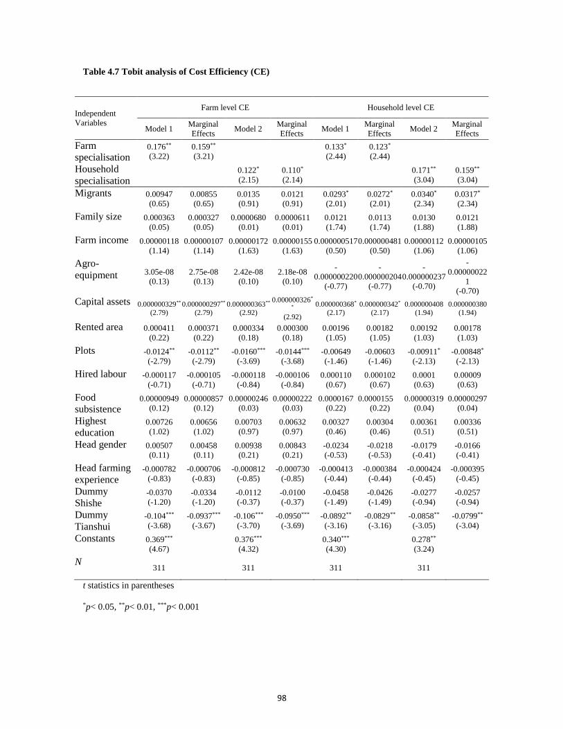
98
Table 4.7 Tobit analysis of Cost Efficiency (CE)
Independent
Variables
Farm level CE Household level CE
Model 1 Marginal
Effects Model 2
Marginal
Effects Model 1
Marginal
Effects Model 2
Marginal
Effects
Farm
specialisation 0.176**
(3.22)
0.159**
(3.21)
0.133*
(2.44)
0.123*
(2.44)
Household
specialisation
0.122*
(2.15)
0.110*
(2.14)
0.171**
(3.04)
0.159**
(3.04)
Migrants 0.00947
(0.65)
0.00855
(0.65)
0.0135
(0.91)
0.0121
(0.91)
0.0293*
(2.01)
0.0272*
(2.01)
0.0340*
(2.34)
0.0317*
(2.34)
Family size 0.000363
(0.05)
0.000327
(0.05)
0.0000680
(0.01)
0.0000611
(0.01)
0.0121
(1.74)
0.0113
(1.74)
0.0130
(1.88)
0.0121
(1.88)
Farm income 0.00000118
(1.14)
0.00000107
(1.14)
0.00000172
(1.63)
0.00000155
(1.63)
0.000000517
(0.50)
0.000000481
(0.50)
0.00000112
(1.06)
0.00000105
(1.06)
Agro-
equipment 3.05e-08
(0.13)
2.75e-08
(0.13)
2.42e-08
(0.10)
2.18e-08
(0.10)
-
0.000000220
(-0.77)
-
0.000000204
(-0.77)
-
0.000000237
(-0.70)
-
0.00000022
1
(-0.70)
Capital assets 0.000000329** (2.79)
0.000000297** (2.79)
0.000000363** (2.92)
0.000000326*
*
(2.92)
0.000000368* (2.17)
0.000000342* (2.17)
0.000000408 (1.94)
0.000000380 (1.94)
Rented area 0.000411
(0.22)
0.000371
(0.22)
0.000334
(0.18)
0.000300
(0.18)
0.00196
(1.05)
0.00182
(1.05)
0.00192
(1.03)
0.00178
(1.03)
Plots -0.0124**
(-2.79)
-0.0112**
(-2.79)
-0.0160***
(-3.69)
-0.0144***
(-3.68)
-0.00649
(-1.46)
-0.00603
(-1.46)
-0.00911*
(-2.13)
-0.00848*
(-2.13)
Hired labour -0.000117
(-0.71)
-0.000105
(-0.71)
-0.000118
(-0.84)
-0.000106
(-0.84)
0.000110
(0.67)
0.000102
(0.67)
0.0001
(0.63)
0.00009
(0.63)
Food
subsistence 0.00000949
(0.12)
0.00000857
(0.12)
0.00000246
(0.03)
0.00000222
(0.03)
0.0000167
(0.22)
0.0000155
(0.22)
0.00000319
(0.04)
0.00000297
(0.04)
Highest
education 0.00726
(1.02)
0.00656
(1.02)
0.00703
(0.97)
0.00632
(0.97)
0.00327
(0.46)
0.00304
(0.46)
0.00361
(0.51)
0.00336
(0.51)
Head gender 0.00507
(0.11)
0.00458
(0.11)
0.00938
(0.21)
0.00843
(0.21)
-0.0234
(-0.53)
-0.0218
(-0.53)
-0.0179
(-0.41)
-0.0166
(-0.41)
Head farming
experience -0.000782
(-0.83)
-0.000706
(-0.83)
-0.000812
(-0.85)
-0.000730
(-0.85)
-0.000413
(-0.44)
-0.000384
(-0.44)
-0.000424
(-0.45)
-0.000395
(-0.45)
Dummy
Shishe -0.0370
(-1.20)
-0.0334
(-1.20)
-0.0112
(-0.37)
-0.0100
(-0.37)
-0.0458
(-1.49)
-0.0426
(-1.49)
-0.0277
(-0.94)
-0.0257
(-0.94)
Dummy
Tianshui -0.104***
(-3.68)
-0.0937***
(-3.67)
-0.106***
(-3.70)
-0.0950***
(-3.69)
-0.0892**
(-3.16)
-0.0829**
(-3.16)
-0.0858**
(-3.05)
-0.0799**
(-3.04)
Constants 0.369***
(4.67)
0.376***
(4.32)
0.340***
(4.30)
0.278**
(3.24)
N 311 311 311 311
t statistics in parentheses
*p< 0.05, **p< 0.01, ***p< 0.001
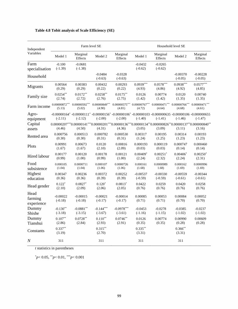
99
Table 4.8 Tobit analysis of Scale Efficiency (SE)
Independent
Variables
Farm level SE Household level SE
Model 1 Marginal
Effects Model 2
Marginal
Effects Model 1
Marginal
Effects Model 2
Marginal
Effects
Farm
specialisation -0.100
(-1.39)
-0.0681
(-1.38)
-0.0432
(-0.62)
-0.0265
(-0.62)
Household -0.0484
(-0.63)
-0.0328
(-0.63)
-0.00370
(-0.05)
-0.00228
(-0.05)
Migrants 0.00564
(0.29)
0.00383
(0.29)
0.00432
(0.22)
0.00293
(0.22)
0.0939***
(4.93)
0.0578***
(4.86)
0.0938***
(4.92)
0.0577***
(4.85)
Family size 0.0254**
(2.74)
0.0172**
(2.72)
0.0258**
(2.76)
0.0175**
(2.75)
0.0126
(1.42)
0.00774
(1.42)
0.0120
(1.35)
0.00740
(1.35)
Farm income 0.00000872***
(5.13)
0.00000592***
(5.02)
0.00000849***
(4.90)
0.00000575***
(4.81)
0.00000767***
(4.72)
0.00000471***
(4.64)
0.00000766***
(4.68)
0.00000471***
(4.61)
Agro-
equipment -0.00000164*
(-2.11)
-0.00000111*
(-2.12)
-0.00000156*
(-2.00)
-0.00000106*
(-2.00)
-0.00000103
(-1.40)
-0.000000635
(-1.41)
-0.00000106
(-1.46)
-0.000000655
(-1.47)
Capital
assets 0.00000207***
(4.46)
0.00000141***
(4.50)
0.00000201***
(4.31)
0.00000136***
(4.36)
0.00000134**
(3.05)
0.000000826**
(3.09)
0.00000137**
(3.11)
0.000000840**
(3.16)
Rented area 0.000756
(0.30)
0.000513
(0.30)
0.000782
(0.31)
0.000530
(0.31)
0.00317
(1.24)
0.00195
(1.25)
0.00314
(1.23)
0.00193
(1.23)
Plots 0.00991
(1.67)
0.00673
(1.67)
0.0120
(2.10)
0.00816
(2.09)
0.000193
(0.03)
0.000119
(0.03)
0.000747
(0.14)
0.000460
(0.14)
Hired labour 0.00177
(0.99)
0.00120
(1.00)
0.00178
(0.99)
0.00121
(1.00)
0.00409*
(2.24)
0.00251*
(2.32)
0.00406*
(2.24)
0.00250*
(2.31)
Food
subsistence 0.000105
(1.04)
0.0000711
(1.04)
0.000107
(1.06)
0.0000726
(1.06)
0.000161
(1.68)
0.0000989
1.68)
0.000162
(1.69)
0.0000996
(1.69)
Highest
education 0.00347
(0.36)
0.00236
(0.36)
0.00372
(0.39)
0.00252
(0.39)
-0.00537
(-0.59)
-0.00330
(-0.59)
-0.00559
(-0.61)
-0.00344
(-0.61)
Head gender 0.122*
(2.10)
0.0827*
(2.09)
0.120*
(2.06)
0.0813*
(2.05)
0.0422
(0.76)
0.0259
(0.76)
0.0420
(0.76)
0.0258
(0.76)
Head
farming
experience
-0.00022
(-0.18)
-0.00015
(-0.18)
-0.00021
(-0.17)
-0.00014
(-0.17)
0.00085
(0.71)
0.00053
(0.71)
0.00084
(0.70)
0.00052
(0.70)
Dummy
Shishe -0.130**
(-3.18)
-0.0881**
(-3.15)
-0.144***
(-3.67)
-0.0978***
(-3.61)
-0.0453
(-1.16)
-0.0278
(-1.15)
-0.0385
(-1.02)
-0.0237
(-1.02)
Dummy
Tianshui 0.107**
(2.86)
0.0728**
(2.84)
0.110**
(2.93)
0.0746**
(2.91)
0.0126
(0.35)
0.00774
(0.35)
0.00990
(0.28)
0.00609
(0.28)
Constants 0.337**
(3.19)
0.315**
(2.70)
0.335**
(3.31)
0.366**
(3.31)
N 311 311 311 311
t statistics in parentheses
*p< 0.05, **p< 0.01, ***p< 0.001

100
Table 4.9 Regression of farm income on efficiency measures
Explanatory variables Model
1 2
Intercept -15893 -17768
Cost efficiency 4885(1.03) ---
Technical efficiency --- 8801(1.78)
Allocative efficiency --- 2021(0.40)
Scale efficiency 26637** (8.55) 28118**(8.79)
Farm-type dummy (specialized=1)# 10081**(4.92) 8689**(4.00)
n 317 317 2R 0.41 0.38
Note: # Specialised farms are identified as for those the specialisation index0.5
Numbers in parentheses are T values *P< 0.05, ** p< 0.01
101
Chapter 5
Conclusion and policy implication
Chapters 2, 3 and 4 provided analyses of regional diversification in agriculture, the farm-
level specialisation and commercialisation, and the impact of production specialisation on
economic efficiencies. The goal was to answer the following questions, which refer to
this thesis’s hypotheses: Is the agricultural sector in the less-favoured regions
diversifying as per the general trend of the whole country (H1)?Does market participation
lead to higher-level production specialisation (H2)? Are specialised small farms
economically efficient (H3)?
The results of this study offer a reminder of the central role of agriculture in China’s
growth process, and its importance as a contributor to poverty alleviation. Combining
various data source with multiple methods, this research shows that rural households
have moved from diversified to specialised activities to respond to market development,
and identifies the trade-offs of this shift in terms of productivity and efficiency.
5.1 Conclusion
5.1.1 China’s structural change and agricultural diversification
China’s rapid growth and its special paths of transition and development have puzzled
scholars looking at the contradictions between expectations shaped by theory and the
observed outcomes (Jefferson, 2008). In terms of structural change and agricultural
transformation, the aggregate-level analyses of this study suggest that, although
economic growth in China is unique, its pattern of agricultural transformation is
102
consistent with structural change theory and the experiences of other developing
countries. China’s agricultural sector becomes more diversified as the economy grows.
Among regions, the degree of agricultural diversification appears to relate to a region’s
comparative advantage and the relative importance of agriculture in the region. A specific
provincial-level analysis reveals that environmentally and economically disadvantaged
regions are slower to diversify their economy than are better endowed regions. The
sectoral composition of the wider economy in the early stage of transformation also
affects agricultural transformation and diversification. Insights from the investigation into
the underdeveloped Gansu province suggest that if a region’s economy relies heavily on
state-owned enterprises, its rural economy is likely to experience higher initial barriers to
labour mobility. These barriers significantly slow the process of agricultural
diversification.
5.1.2 Smallholder specialisation and commercialisation: an interplay
Results from econometric modelling suggest that smallholders’ agricultural
commercialisation is interrelated to production specialisation. Commercialisation leads to
specialisation, and specialised farms are much more commercial-based and market a
higher percentage of their produce.
The strong two-way interrelationship found by this study suggests that farmers’ decisions
on farm commercialisation and production specialisation are actually separate and
interacting. The insights of this study show those two activities facilitate each other, and
respond to other exogenous factors differently in different processes. The findings cast
103
further light onto the farm market participation theory by emphasising that higher asset
endowments enable small farmers to specialise in production with comparative advantage.
Commercialising the small subsistence farms in underdeveloped rural areas is
fundamental to reducing China’s regional development disparity. This study shows that
facilitating production specialisation can indirectly stimulate smallholders’ agricultural
commercialisation. The interplay between commercialisation and specialisation can be
used by policy-makers to combine market improvement and risk management tools to
more effectively increase farmers’ income.
5.1.3 Specialisation of small farms: the gain in production efficiency
This research reveals that specialisation increases households’ technical efficiency and
cost efficiency. The results confirm that specialised farms benefit from a decreasing
average cost per unit of output or increasing outputs. These benefits are partly explained
by either the effect of learning-by-doing, or the effect of economies of scale. Analyses of
households’ characteristics show that food-secure households are likely to be technically
efficient, but technical efficiency is hindered by losing product to relatively more
productive workers, while land fragmentation has adverse effects on technical and cost
efficiencies.
Across the three study areas, economic losses are commonly generated by allocative and
scale inefficiency. Although farms are relatively technically efficient, labour, fertiliser
and seed are overused among the inefficient farms. The allocative inefficiency represents
a failure to respond to price and resource scarcity in household decision-making.
Evidence of inefficiency in labour allocation between farm and non-farm activities is also
104
found. Most farms are identified as operating under increasing returns-to-scale, indicating
that economies of scale exist in local agriculture and efficiency can be improved by
enlarging the scale of operation.
5.2 Policy implications
The results of this study contribute to debates on China’s rural transformation process
and provide an outline for understanding the progressing tendencies and the macro-micro
links of diversification and specialisation. The findings further show the significance of
regional comparative advantages (for example, natural endowments, market functionality,
and the activity of non-state-owned enterprises) that determine how much a region can
transfer its labour out of agriculture, and how quickly this region can narrow the gap
between agriculture’s share of GDP and increasing employment to reduce poverty and
rural-urban disparity. This research provides insights into the specific circumstances of
farmers in less-favoured regions, demonstrated by the surveyed households in the Gansu
province of Western China, where the region is still in an early stage of the economic
transition, and the smallholders could be constrained from increasing their incomes and
integrating into the restructuring of agro-food markets.
Although in a relatively early stage of agricultural transformation, farmers in Western
China are apparently influenced by market liberalisation and integration. They are
shifting away from mixed subsistence farming and specialising in less on-farm and more
off-farm activities for their livelihood, and the specialisation is positively related to
farmers’ market participation. It is well recognised that smallholders’ commercialisation
and on-farm specialisation is a pathway out of poverty. However, governments,
105
especially those in less-favoured areas, usually struggle to deliver effective policy
practice to make the majority of small farms integrate into the market. The “virtuous
cycle” between farmers’ commercialisation and specialisation found in this study
provides new insights into the small farms’ commercialisation process, and thereby offers
moderate guidance for policy implementation. It emphasises that farmers’ market
participation can be indirectly improved by implementing policies that encourage
specialisation, and to open an alternative policy channel for enhancing commercialisation.
Smallholder farming has been promoted in China to deliver incentives, efficiency and
equity. However, the new technology-driven markets, with demand for high-value and
processed products, challenge smallholders with quality, timely deliveries, and
economies of scale (World Bank, 2007). This research confirms that the economic losses
are commonly generated by allocative and scale inefficiency, and some farmers are not at
their optimal scales. As most of the farmers are operating at increasing return-to-scale,
economics of scale can be captured in local agriculture, and enlargement of operation
scale can be a means of improving efficiency.
To implement the agriculture-for-development agenda, the promotion of high-value farm
activities and non-farm employment, and the provision of infrastructure to support
diversification in agriculture and rural economies are recommended policies. The insights
of this research clarify that a discussion of patters of agricultural
diversification/specialisation, and the strategy of agriculture-for-development, must be
region and settings-specific. For the less-favoured smallholder in Western China, a more
effective strategy might be to establish efficient value chains, enhance smallholders’
competitiveness and facilitate their market access. By improving markets, especially the
106
missing institutions for credit, technical support and insurance, smallholders can be
encouraged to specialise in high-value activities and integrate into the market. As this
research shows, the interaction between specialisation and commercialisation not only
leads to a “virtuous cycle” of income generation, but also increases farm production
efficiency.
5.3 Limitations of the study
The aim of the this thesis was to have a thorough and comprehensive understanding of
agricultural transformation in China. To achieve this goal, at the macro level, the study
identifies the primary similarities and differences in China’s processes of adaptation to
the new context of structural change; at the micro level, it focuses on farm diversification
to specialisation and the impacts of specialisation on efficiency. This all structure-
dimensions study which fully considers micro-foundations with macro phenomenon,
however, was bound to be challenging. To rigorously demonstrate the processes of
change in agriculture at different levels, historical and consistent data at national,
regional and household levels are required, which was very difficult to obtain. The lack
of consistent data led to the first limitation of this study: a single case study of Gansu
province was only superficially studied, which makes the provincial-level analysis
ineffective to the interpretation of results. If one more provincial-level case could draw
from a typical macro-region, an in-depth analysis would have been conducted in
examining the contextual specificities of the two provinces and of how their economic
and institutional characteristics have evolved over the course of the reforms.
Second, identifying explanatory factors in agricultural transformation and evaluating
107
impacts of diversification/specialisation on income and productivity, face both
information difficulties, as well as a risky discussion on the direction of causality(Losch,
Fréguin-Gresh, & White, 2012).This is also true for the current study, due to limitations
of project duration and funding, only cross-sectional data were able to be collected on
household level analysis. As a result, the analysis of two-way relationship between
commercialisation and specialisation might be open to debate, although the 2SLS and
3SLS were used to deal with simultaneous issues, and the relevant diagnostic statistical
tests were appropriately employed. When household panel data is available, a further
study should be conducted with a much more sophisticated method to investigate the
impacts and causality of income levels and diversification/specialization patterns.
108
References
Acharya, S. P., Basavaraja, H., Kunnal, L. B., Mahajanashetti, S. B., & Bhat, A. R. (2011). Crop diversification
in Karnataka: An economic analysis.Agricultural Economics Research Review, 24(2).
Alemu, D. (2007). Determinants of smallholder commercialization of food crops: Theory and evidence
from Ethiopia(Vol. 745). Intl Food Policy Res Inst.
Ali, M., & Chaudhry, M. (1990). Inter‐regional farm efficiency in Pakistan's Punjab: a frontier Production
function study.Journal of Agricultural Economics, 41(1), 62-74.
Aly, H., Belbase, K., Grabowski, R.,& Kraft, S. (1987). The technical efficiency of Illinois grain farms: An
application of a ray-homothetic production function.Southern Journal of Agricultural Economics,
19 (1), 69-78.
Arrighi,Giovanni (2007), Adam Smith in Beijing: Lineages of the XXI Century. London: Verso
Ash, R. (1988). The Evolution of Agricultural Policy.The China Quarterly, 116, 529-555.
doi:10.1017/S0305741000037887.
Asset, B. A. (2012). Income diversificationsamong african agriculturalist: some practical issues,” project
report to USAID BASIS CRSP.
Bagi, F. (1982). Relationship between farm size and technical efficiency in West Tennessee
agriculture.Southern Journal of Agricultural Economics,14 (2).
Barrett, C. (2008). Smallholder market participation: concepts and evidence from eastern and southern
Africa. Food Policy, 33 (4), 299-317.
Barrett, C.B., Bachke, M.E., Bellemare, M.F., Michelson, H.C., Narayanan, S., Walker, T.F., 2012.
Smallholder participation in contract farming: comparative evidence from five countries. World
Dev. 40 (4), 715–730.
Belbase, K., & Grabowski, R. (1985). Technical efficiency in Nepalese agriculture. The Journal of Developing
Areas, 515-526.
Bellotti, B. (2006). Improving the productivity and sustainability of rainfed farming systems for the Loess
Plateau of Gansu Province.http://hdl.handle.net/2440/40721
109
Benjamin, D., & Brandt, L. (2002). Property Rights, Labour Markets, and Efficiency in A Transition Economy:
The Case of Rural China. Canadian Journal of Economics/Revue canadienne d'économique, 35 (4), 689-716.
Benni, N. E., Finger, R., & Mann, S. (2012). Effects of agricultural policy reforms and farm characteristics
on income risk in swiss agriculture. Agricultural Finance Review, 72(3), 301-324.
doi:http://dx.doi.org.ezproxy.uws.edu.au/10.1108/00021461211277204
Berry, R. A., & Cline, W. R. (1979). Agrarian structure and productivity in developing countries: a study
prepared for the International Labour Office within the framework of the World Employment
Programme. Johns Hopkins Univ. Press.
Bharati, P., De, U. K., & Pal, M. (2015). A modified diversity index and its application to crop diversity in
Assam, India. AIP Conference Proceedings (Vol.1643, pp.19-29).
Baumgartner, P., Braun, J. V., Abebaw, D., & Müller, M. (2015). Impacts of large-scale land investments on
income, prices, and employment: empirical analyses in ethiopia. World Development, 72, 175-
190.
Brandt, L., Hsieh C-T., & Zhu, X. (2008). Growth and Structural Transformation in China.China’s great
economic transformation,683-728.
Brandt, L., & Rawski, T. G. (2008). China's Great Economic Transformation. Cambridge University Press.
Branstetter, L., & Lardy, N. (2006). China's Embrace of Globalization. National Bureau of Economic
Research.
Bravo-Ureta, B.,& Evenson, R.(1994). Efficiency in agricultural production: the case of peasant farmers in
Eastern Paraguay.Agricultural economics, 10 (1), 27-37.
Bravo-Ureta, B., & Pinheiro, A.(1993). Efficiency analysis of developing country agriculture: a review of the
frontier function literature. Agricultural and Resource Economics Review,22 (1), 88-101.
Brown, C., & Kai, C. (1999). Land reform, household specialisation and rural development in China.
Agricultural and Natural Resource Economics Discussion Paper 8.
Brown, C., Waldron, S., Liu, Y.,& Longworth, J. (2009). Forage-livestock policies designed to improve
livelihoods in Western China: a critical review. China Agricultural Economic Review,1 (4), 367-381.
doi: http://dx.doi.org/10.1108/17561370910989220.
110
Brown, C., Waldron, S., Yuman, L.,& Longworth, J. (2009). Forage-Livestock Policies Designed to Improve
Livelihoods in Western China: A Critical Review. China Agricultural Economic Review,1 (4), 367-
381.
Byrnes, P., Färe, R., Grosskopf, S.,& Kraft, S. (1987). Technical efficiency and size: the case of Illinois grain
farms. European Review of Agricultural Economics, 14(4), 367-381.
Cameron, A. C., & Trivedi, P. K. (2010). Microeconometrics using stata.
Carter, C., & Lohmar, B. (2002). Regional Specialization of China's Agricultural Production. American
Journal of Agricultural Economics, 84 (3), 749-753. doi:10.2307/1244849.
Carter, C., Zhong, F.,& Zhu, J. (2012). Advances in Chinese Agriculture and its Global Implications. Applied
Economic Perspectives & Policy,34(1), 1-36.
Chavas, J-P. (2001). Structural change in agricultural production: Economics, technology and policy.
Handbook of agricultural economics,1,263-285.
Chavas, J-P., & Aliber, M. (1993). An analysis of economic efficiency in agriculture: a nonparametric
approach. Journal of Agricultural and Resource Economics, 1-16.
Chavas, J-P, Petrie, R., & Roth, M. (2005). Farm household production efficiency: evidence from the
Gambia.American Journal of Agricultural Economics,87 (1), 160-179.
Chavas, J‐P. (2008). On the economics of agricultural production*. Australian Journal of Agricultural and
Resource Economics,52(4), 365-380.
Chen, Z., Huffman, W., & Rozelle, S. (2009). Farm technology and technical efficiency: Evidence from four
regions in China. China Economic Review,20(2), 153-161.
Chenery, H. (1988). Patterns of Development. Beijing: Economics Science Press.
Coelli, T., & Fleming, E. (2004). Diversification Economies and Specialisation Efficiencies in A Mixed Food
and Coffee Smallholder Farming System in Papua New Guinea. Agricultural Economics, 31(2-3),
229-239. doi: 10.1111/j.1574-0862.2004.tb00260.x.
Coelli, T., Rao, D., O'Donnell, C.,& Battese, G. (2005). An introduction to efficiency and
productivity analysis. Springer Science & Business Media.

111
Coelli, T., & Battese, G. (1996). Identification of Factors Which Influence The Technical Inefficiency of
Indian Farmers. Australian Journal of Agricultural Economics, 40(2), 103-128. doi:10.1111/j.1467-
8489.1996.tb00558.x.
Coelli, T., Rahman, S.,& Thirtle, C. (2002). Technical, Allocative, Cost and Scale Efficiencies in Bangladesh
Rice Cultivation: A Non‐parametric Approach. Journal of Agricultural Economics,53(3), 607-626.
Colander, D. (2013). MACROECONOMICS. McGraw Hill Higher Education.
Culas, R. (2006a). Causes of farm diversification over time: an Australian perspective on an Eastern
Norway model. Australian Farm Business Management Journal,3(1), 1.
Deininger, K., Jin, S., Xia, F.,& Huang, J. (2013). Moving off the farm: Land institutions to facilitate
structural transformation and agricultural productivity growth in China. World Development.
Dorsey, B. (1999). Agricultural Intensification, Diversification, and Commercial Production among
Smallholder Coffee Growers in Central Kenya. Economic Geography, 75(2), 178-195.
doi:10.2307/144250.
Dorsey, E., Jarjoura, D., & Rutecki, G. (2005). The influence of controllable lifestyle and sex on the
specialty choices of graduating US medical students, 1996-2003. Academic Medicine,80(9), 791-
796.
Dube, L. (2016). Factors influencing smallholder crop diversification: a case study of manicaland and
masvingo provinces in zimbabwe. , 3(2), 1.
Eastwood, R., Lipton, M., & Newell, A. (2010). Farm size. Handbook of agricultural economics,4, 3323-
3397.
Emran, M., & Shilpi, F. (2012). The Extent of The Market and Stages of Agricultural Specialization.
Canadian Journal of Economics/ Revue canadienne d'économique,45(3), 1125-1153.
doi:10.1111/j.1540-5982.2012.01729.x.
Färe, R., Grosskopf, S., & Logan, J. (1985). The relative performance of publicly-owned and privately-
owned electric utilities.Journal of Public Economics,26(1), 89-106. doi:10.1016/0047-
2727(85)90040-4.
Färe, R., Grosskopf, S. and Lovell, C. (1994). Production Frontiers. Cambridge: Cambridge University Press.
112
Färe, R., & Lovell, C. (1978). Measuring the technical efficiency of production.Journal of Economic
Theory,19(1). 150-162. doi:10.1016/0022-0531(78)90060-1.
Fan, S. (2000). Technological change, technical and allocative efficiency in Chinese agriculture: the case of
rice production in Jiangsu. Journal of International Development,12 (1), 1-12.
Fan, S. (2006). Rural Development Strategy in Western China Under the WTO. In S. Song, X. Zhang, & X. Y.
Dong (Eds.) China's Agricultural Development: Challenges and prospects. Aldershot: Ashgate.
Fan, S, Zhang, X., & Robinson, S. (2003). Structural Change and Economic Growth in China. Review of
Development Economics,7(3), 360-377. doi:10.1111/1467-9361.00196.
Farrell, M. (1957). The measurement of productive efficiency. Journal of the Royal Statistical Society.
Series A (General). 253-290.
Feng, S. (2008). Land rental, off-farm employment and technical efficiency of farm households in Jiangxi
Province, China. NJAS-Wageningen Journal of Life Sciences,55(4), 363-378.
Fernandez-Cornejo, J. (1993). Demand and substitution of agricultural inputs in the central corn belt states.
United States Department of Agriculture, Economic Research Service.
Fleisher, B, & Liu, Y. (1992). Economies of Scale, Plot Size, Human-Capital, and Productivity in Chinese
Agriculture. Quarterly Review of Economics and Finance,32(3), 112-123.
Gansu Yearbook Editorial Board. (2007-2011). Gansu Yearbook. Beijing: China Satistics Press.
Garcia, P., Offutt, S., & Sonka, S. (1987). Size distribution and growth in a sample of Illinois cash grain
farms.American Journal of Agricultural Economics,69(2), 471-476.
Gebreselassie, S., & Ludi, E. (2007). Agricultural Commercialisation in Coffeegrowing Areas of Ethiopia.
Paper read at Fifth International Conference on the Ethiopian Economy, EEA.
Gebreselassie, S., & Sharp, K. (2008). Commercialisation of Smallholder Agriculture in Selected Tef-
growing Areas of Ethiopia.Ethiopian Journal of Economics, 16.
Goletti, F., Purcell, T.,&Smith, D. (2003). Concepts of Commercialization and Agricultural Development.
Agrifood Discussion Paper Series.
Gorton, M., & Davidova, S. (2004). Farm productivity and efficiency in the CEE applicant countries: a
synthesis of results. Agricultural economics,30 (1), 1-16.
113
Govereh, J., & Jayne, T. (2003). Cash cropping and food crop productivity: synergies or trade‐offs?"
Agricultural Economics, 28(1), 39-50.
Gujarati, D. (2008, 2003).Basic Econometrics. International Edition, Mcgraw-Hill.
Haji, J. 2007. Production efficiency of smallholders' vegetable-dominated mixed farming system in Eastern
Ethiopia: A non-parametric approach.Journal of African Economies,16 (1), 1-27.
Hall, B., & E. LeVeen, P. (1978). Farm Size and Economic Efficiency: The Case of California. American
Journal of Agricultural Economics, 60(4), 589-600.
Hansson, H. (2008). Are larger farms more efficient? A farm level study of the relationships between
efficiency and size on specialized dairy farms in Sweden. Agricultural and food science,17(4), 325-
337.
Harvey, David (2005), A Brief History of Neoliberalism. Oxford: Oxford, University Press (especially
Chapter 5, “Neoliberalism with Chinese characteristics”.
Heck, J. (1977). A Pedagogic Note: Comparison of OLS, 2SLS and 3SLS Estimation Methods. Studies in
Economics and Finance, 1(1), 28-33.
Heady, E. (1952). Diversification in resource allocation and minimization of income variability." Journal of
Farm Economics,34(4), 482-496.
Herrmann-Pillath, C. (1994). China’s Transition to The Market: A Paradox of Transformation and Its
Institutionalist Solution. In The Political Economy of Transformation, 209-241: Springer.
Heston, A., & Sicular, T. (2008). China and Development Economics. In L. Brandt & T. G. Rawsk (Eds.),
China’s Great Economic Transformation., (pp. 27-67).
Hofman, B.,& Wu, J. (2009). Explaining China's development and reforms. Citeseer.
Hoff, A. (2007). Second stage dea: comparison of approaches for modelling the dea score. European
Journal of Operational Research, 181(1), 425-435.
Hou, F., Nan, Z.,Xie,Y., Li, X.,Lin, H.& Ren. J.(2008). Integrated crop-livestock production systems in China.
The Rangeland Journal,30(2), 221-231. doi:http://dx.doi.org/10.1071/RJ08018.
Huang, J., Bi, X.,& Rozelle, S. (2004). Market, specialization and China's smallholder agriculture. Food and
agricultural organisation.
114
Huang, J., Otsuka, K., & Rozelle, S. (2008). Agriculture in China’s Development Past Disappointments,
Recent Successes, and Future Challenges. In T. G. Rawski, L. Brandt (Eds.),China’s Great Economic
Transformation, (pp. 467-505). New York: Cambridge
Huang, J., Wang, X.,& Qiu, H. (2012). Small-scale farmers in China in the face of modernisation and
globalisation. London: International Institute for Environment and Development, Small Producer
Agency in the Globalised Market Knowledge Programme.
Huanxian Yearbook Editorial Board. (2013). Huanxian Yearbook. Beijing: China Statistics Press.
Jefferson, G. (2008). How Has China's Economic Emergence Contributed to the Field of Economics?
Comparative Economic Studies, 50(2), 167-209. doi:http://dx.doi.org/10.1057/ces.2008.14.
Jin, S., Huang, J.,& Rozelle, S. (2010). Agricultural productivity in China. In The shifting patterns of
agricultural production and productivity worldwide.
Johnston, B., & Kilby, P. (1975). Agriculture and Structural Transformation; Economic Strategies In Late-
Developing Countries.
Kalaitzandonakes, N., Wu, S.,& Ma,J. (1992). The Relationship between Techinical Efficiency and Firm Size
Revisited." Canadian Journal of Agricultural Economics/Revue canadienne d'agroeconomie,40(3),
427-442.
Kalirajan, K. (1984). Farm-specific technical efficiencies and development policies. Journal of Economic
Studies,11(3), 3-13.
Kalirajan, K. (1981). An econometric analysis of yield variability in paddy production. Canadian Journal of
Agricultural Economics/Revue canadienne d'agroeconomie,29(3), 283-294.
Kalirajan, K. (1990). On measuring economic efficiency. Journal of Applied Econometrics,5(1), 75-85.
Kalirajan, K., & Flinn, J. (1983). The measurement of farm specific technical efficiency. Pakistan Journal of
Applied Economics,2(2), 167-180.
Kalirajan, K., & Shand,R.(1985). Types of education and agricultural productivity: a quantitative analysis of
Tamil Nadu rice farming. The Journal of Development Studies, 21(2), 232-243.
Kimenju, S. C., & Tschirley, D. (2009). Agriculture and livelihood diversification in kenyan rural households.
115
Kim, K., Chavas, J-P., Barham, B., & Foltz, J. (2012). Specialization, Diversification, and Productivity: A Panel
Data Analysis Of Rice Farms In Korea.Agricultural Economics,43(6), 687-700. doi:10.1111/j.1574-
0862.2012.00612.x.
Kumar, S., & Gulati, R. (2008). An examination of technical, pure technical, and scale efficiencies in Indian
public sector banks using data envelopment analysis.Eurasian Journal of Business and
Economics,1(2), 33-69.
Langemeier, M., & Jones, R. (2000). Measuring the impact of farm size and specialization on financial
performance.Journal of the ASFMRA,63(1), 90-96.
Latruffe, L., Balcombe, K., Davidova, S.,& Zawalinska, K. (2005). Technical and scale efficiency of crop and
livestock farms in Poland: does specialization matter? Agricultural economics,32(3), 281-296.
Lau, L., & Yotopoulos, P. (1971). A test for relative efficiency and application to Indian agriculture. The
American Economic Review. 94-109.
Leavy, J., & Poulton, C. (2007). Commercialisations in agriculture: A typology. Paper read at Proceedings of
the fifth international conference on the Ethiopian economy.
Li, L., Wang, C., Segarra, E., & Nan, Z. (2013). Migration, remittances, and agricultural productivity in small
farming systems in Northwest China. China Agricultural Economic Review, 5(1), 5-23.
Lin, J. (1988). The Household Responsibility System in China's Agricultural Reform: A Theoretical and
Empirical Study.Economic Development and Cultural Change,36(3), S199-S224.
doi:10.2307/1566543.
Lin, J. (1992). Rural Reforms and Agricultural Growth in China. The American Economic Review,82(1), 34-
51. doi:10.2307/2117601.
Lin, J., Cai, F.,& Li, Z. (1996). The Lessons of China's Transition to a Market Economy. Cato J.16, 201.
Lin, W., &Shao, B. (2000). The relationship between user participation and system success: a simultaneous
contingency approach. Information & Management,37(6),283-295.
Lin, Y., Dong, Y., Song, S.,& Zhang, X. (2006). Several strategic and political thoughts on boosting rural
development.China's agricultural development: challenges and prospects. 23-32.

116
Lipton, M., & Longhurst, R. (1989). New Seeds and Poor People. Johns Hopkins University Press: Baltimore,
USA.
Liu, J., Li, S., Ouyang, Z., Tam, C., & Chen, X. (208). Ecological and Socioeconomic Effects of China's Policies
for Ecosystem Services." Proceedings of the National Academy of Sciences of the United States of
America,105(28), 9477-9482. doi:10.2307/25462998.
Liu, Z., & Zhuang, J. (2000). Determinants of technical efficiency in post-collective Chinese agriculture:
evidence from farm-level data. Journal of Comparative Economics, 28(3), 545-564.
Losch, B., Fréguin-Gresh, S., & White, E. (2012). Structural transformation and rural change revisited:
challenges for late developing countries in a globalizing world: World Bank Publications.
Mao, W., & Koo, W. (1997). Productivity growth, technological progress, and efficiency change in Chinese
agriculture after rural economic reforms: a DEA approach. China Economic Review,8(2), 157-174.
McCalla, A. (1997). From Subsistence Systems to Commercial Agriculture: The Need for a New
Development Paradigm: Discussion. American Journal of Agricultural Economics,79(2), 643-645
McMillan, J., Whalley, J.,& Zhu, L. (1989). The Impact of China's Economic Reforms on Agricultural
Productivity Growth. Journal of Political Economy,97(4), 781-807. doi:10.2307/1832191.
Mesfin, W., Fufa, B.,& Haji, J. (2011). Pattern, Trend and Determinants of Crop Diversification: Empirical
Evidence from Smallholders in Eastern Ethiopia. Journal of Economics and Sustainable
Development, 2(8), 78-89.
MOA, 2010, Agriculture in China. http://english.agri.gov.cn/overview/201301/t20130128_10644.htm
MOA, 2015, SCIO briefing on agricultural modernization,
http://english.agri.gov.cn/hottopics/cpc/201502/t20150204_24960.htm, source: China.org.cn
Morris, S., Carletto,C., Hoddinott, J.,& Christiaensen, L. (2000). Validity of rapid estimates of household
wealth and income for health surveys in rural Africa. Journal of epidemiology and community
health,54(5), 381-387.
Mugera, A., & Langemeier, M. (2011). Does farm size and specialization matter for productive efficiency?
Results from Kansas. Journal of Agricultural and Applied Economics,43(4), 515.
NBSC. (1978-2012). China Statistics Yearbook. Beijing: China Statistics Press.
117
NBSC. (2004-2012). China Yearbook of Agricultural Price Survey. Beijing: China Statistics Press.
NBSC. (2010). China Statistics Yearbook. Beijing: China Statistics Press.
NBSC. (2013). China Statistics Yearbook. Beijing: China Statistics Press.
Nolan, S., Unkovich, M., Yuying, S., Lingling, Li.,& Bellotti, W. (2008). Farming Systems of The Loess Plateau,
Gansu Province, China. Agriculture, Ecosystems & Environment,124(1–2), 13-23. doi:
http://dx.doi.org/10.1016/j.agee.2007.08.009.
OECD. (2001). Adoption of technologies for sustainable farming systems (the Wageningen Workshop).
Paris: OECD Publications Service.
Oi, J. C. (1999). Two decades of rural reform in China: An overview and assessment. The China Quarterly,
159, 616-628
Ogundari K.(2013) Crop diversification and technical efficiency in food crop production: A study of peasant
farmers in Nigeria[J]. International Journal of Social Economics, , 40(3):267-288.
Omamo, S. (1998). Farm‐To‐Market Transaction Costs and Specialisation in Small‐Scale Agriculture:
Explorations With A Non‐Separable Household Model. The Journal of Development Studies,35(2),
152-163. doi:10.1080/00220389808422568.
Peterson, W., & Kislev, Y. (1991). Economies of Scale in Agriculture: A re-examination of the Evidence.Staff
Paper, 43, 91.
Phillips, J., & Marble, R.(1986). Farmer education and efficiency: a frontier production function
approach.Economics of Education Review,5(3), 257-264.
Pingali, P. (1997). From Subsistence to Commercial Production Systems: The Transformation of Asian
Agriculture.American Journal of Agricultural Economics,79(2), 628-634. doi:10.2307/1244162.
Pingali, P., & Rosegrant, M. (1995). Agricultural Commercialization and Diversification: Processes and
Policies.Food Policy,20(3), 171-185. doi:http://dx.doi.org/10.1016/0306-9192(95)00012-4.
Pope, R., & Prescott, R. (1980). Diversification in Relation to Farm Size and Other Socioeconomic
Characteristics. American Journal of Agricultural Economics,62(3), 554-559.
Preckel, P., Akridge, J.,& Boland, M. (1997). Efficiency measures for retail fertilizer dealers.
Agribusiness,13(5), 497-509.
118
Prosterman, R., Hanstad, T.,& Li, P. (1994). Reforming China's Rural Land System: A Field Report. Rural
Development Institute.
Qingyang Yearbook Editorial Board. (1994-2011). Qingyang Yearbook. China Statistics Press.
Rahman, S. (2009). Whether crop diversification is a desired strategy for agricultural growth in
Bangladesh?Food Policy,34(4), 340-349.
Rios, A., Shively,G.,& Masters, W. (2009). Farm productivity and Household Marekt participation: Evidence
from LSMS Data.International Association of Agricultural Economists Conferenc.Beijing.
Rozelle, S., JiKun, H., Dong, X., Song, S., and Zhang, X. (2006). China's Rural Economy and The Path to A
Modern Industrial State. China's agricultural development: challenges and prospects. 43-77.
Schultz, T. (1964). Transforming traditional agriculture. Transforming traditional agriculture.
Shapiro, K., & Müller, J. (1977). Sources of Technical Efficiency: The Roles of Modernization and
Information.Economic Development and Cultural Change,25(2), 293-310.
Shete, M., & Rutten, M. (2015). Impacts of large-scale farming on local communities’ food security and
income levels – empirical evidence from oromia region, ethiopia. Land Use Policy, 47, 282-292.
Syrquin, M. (1988). Patterns of Structural Change. In Handbook of development economics, (pp. 203-273).
Syrquin, M. (2006). Structural Transformation. The Elgar Companion to Development Studies, Edward
Elgar Publishers,601-607. Cheltenham, UK.
Taylor, J., & Wyatt, T. (1996). The shadow value of migrant remittances, income and inequality in a
household‐farm economy. The Journal of Development Studies, 32(6), 899-912.
Timmer, C. (2002). Agriculture and economic development.Handbook of agricultural economics, 2, 1487-
1546.
Timmer, C. (2009). A World Without Agriculture: The Structural Transformation in Historical Perspective:
AEI Press.
Timmer, C., & Akkus, S. (2008). The structural transformation as a pathway out of poverty: analytics,
empirics and politics. Center for Global Development Working Paper. 150.
Timmer, C. (1988). The Agricultural Transformation.Handbook of development economics, 1(Part II), 276-
331
119
Timmer, C. (1997). Farmers and Markets: The Political Economy of New Paradigms. American Journal of
Agricultural Economics,79(2), 621-627.
Timmer, C. (2007). The Structural Transformation and The Changing Role of Agriculture in Economic
Development: Empirics and Implications. Wendt Lecture, presented to the American Enterprise
Institute, 30.Washington, DC.
Tipraqsa, P., & Schreinemachers, P. (2009). Agricultural commercialization of Karen Hill tribes in northern
Thailand.Agricultural Economics, 40(1), 43-53.
Tobin, J. (1958). Estimation of relationships for limited dependent variables.Econometrica: journal of the
Econometric Society, 24-36.
Tweeten, L. (1984). Causes and consequences of structural change in the farming industry. National
Planning Association.
Udoh, E., Akpan, S.,&Effiong, E. (2011). Economic Analysis of Land Allocation Use and Intensification
among Arable Crop Farmers in Uruan Local Government Area of Akwa-Ibom State,
Nigeria.Journal of Economics and Sustainable Development, 2(11&12), 1-10.
United Nations. (2006). World Economic and Social Survey - Diverging Growth and Development. New
York: Pearson Education.
von Braun, J. (1995). Agricultural Commercialization: Impacts On Income and Nutrition and Implications
For Policy. Food Policy,20(3), 187-202. doi:http://dx.doi.org/10.1016/0306-9192(95)00013-5.
von Braun, J., de Hean, H.,& Blanken, J. (1991). Commercialization of agriculture under population
pressure: Effects on production, consumption, and nutrition in Rwanda, 85. Intl Food Policy Res
Inst.
Wan, G., & Cheng, E. (2001). Effects of land fragmentation and returns to scale in the Chinese farming
sector. Applied Economics,33(2), 183-194.
Wang, J., Wailes, E., & Cramer, G. (1996). A shadow-price frontier measurement of profit efficiency in
Chinese agriculture. American Journal of Agricultural Economics, 78(1), 146-156.
White, T., & Irwin, G. (1972). Farm size and specialization. InA.G. Ball & E.O. Heady (Eds.),Size, Structure
and Future of Farms. Ames: Iowa State University Press.
120
Wickramasinghe, U., & Weinberger, K. (2013). Smallholder Market Participation and Production
Specialisation. Centre for Alleviation of Poverty through Sustainable Agriculture.
Wiens, T. (1987). Issues in the structural reform of Chinese agriculture. Journal of Comparative Economics,
11(3), 372-384.
World Bank. (1986). Growth and development in Gansu province
World Bank. (1988). Diversification in Rurual Asia. The World Bank:Washington, DC.
World Bank. (1990). Agricultural Diversification: Policies and Issues From East Asian Experience. In Policy
and research series. The World Bank:Washington, DC.
World Bank. (1992). Trends in Agricultural Diversification: Regional Perspectives.The World Bank
Washington, D.C.
World Bank. (1997). Implementation completion report: China, Gansu provincial development project.
Report No. 16421-CHA
World Bank. (2007). World development report 2008: Agriculture for development. The World
Bank:Washington, D.C.
World Bank. (2013). World Development Indicators.
World Bank. (2015). World Bank Indicators.
Wu, S., & Prato, T. (2006). Cost efficiency and scope economies of crop and livestock farms in Missouri.
Journal of Agricultural and Applied Economics,38(3), 539.
Xifeng Yearbook Editorial Board. (2013). Xifeng Yearbook. Beijing: China Statistics Press.
Xu, X., & Jeffrey, S. (1998). Efficiency and technical progress in traditional and modern agriculture:
evidence from rice production in China. Agricultural economics,18(2),157-165.
Young, A. (2000). The Razor's Edge: Distortions and Incremental Reform in The People's Republic of
China.The Quarterly Journal Of Economics, CXV(4).
Yue, M.(2009). Empirical Research in the Dynamic Impact of Economic Structure Changes on Economic
Growth since Reform and Opening Up in Gansu. Northwest Normal University.
Zhang, Y., Wang, X., Glauben, T.,& Brümmer, B. (2011). The impact of land reallocation on technical
efficiency: evidence from China. Agricultural Economics. 2(4), 495-507.

121
Zuo, Y., Ma, L., Cai, H., Wu, T., & Xin, X. (2015). China’s on-going debates over large-scale farming: what
are the pros and cons?. China Agricultural Economic Review, 7(3), 338-343.
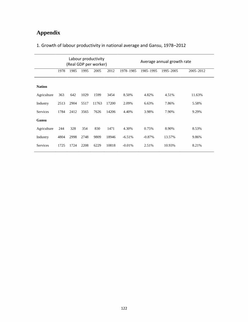
122
Appendix
1. Growth of labour productivity in national average and Gansu, 1978–2012
Labour productivity
(Real GDP per worker) Average annual growth rate
1978 1985 1995 2005 2012 1978–1985 1985–1995 1995–2005 2005–2012
Nation
Agriculture 363 642 1029 1599 3454 8.50% 4.82% 4.51% 11.63%
Industry 2513 2904 5517 11763 17200 2.09% 6.63% 7.86% 5.58%
Services 1784 2412 3565 7626 14206 4.40% 3.98% 7.90% 9.29%
Gansu
Agriculture 244 328 354 830 1471 4.30% 0.75% 8.90% 8.53%
Industry 4804 2998 2748 9809 18946 -6.51% -0.87% 13.57% 9.86%
Services 1725 1724 2208 6229 10818 -0.01% 2.51% 10.93% 8.21%
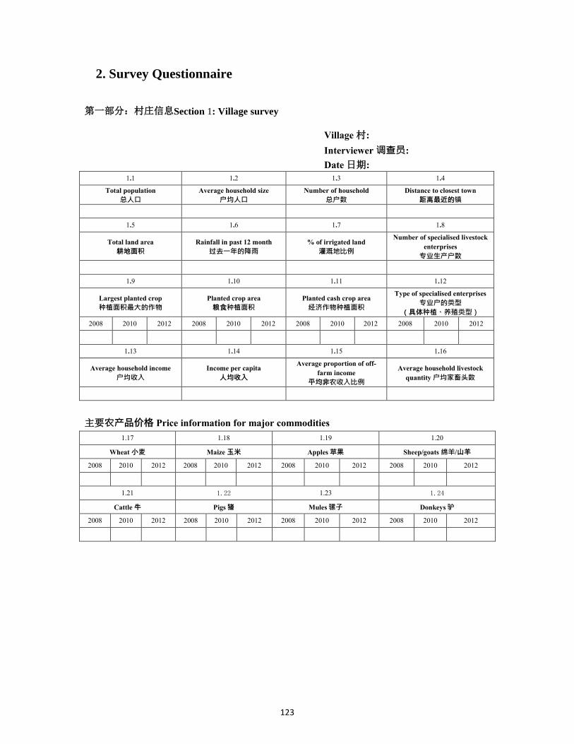
123
2. Survey Questionnaire
第一部分:村庄信息Section 1: Village survey
Village 村:
Interviewer 调查员:
Date 日期:
1.1 1.2 1.3 1.4
Total population
总人口
Average household size
户均人口
Number of household
总户数
Distance to closest town
距离最近的镇
1.5 1.6 1.7 1.8
Total land area
耕地面积
Rainfall in past 12 month
过去一年的降雨
% of irrigated land
灌溉地比例
Number of specialised livestock
enterprises
专业生产户数
1.9 1.10 1.11 1.12
Largest planted crop
种植面积最大的作物
Planted crop area
粮食种植面积
Planted cash crop area
经济作物种植面积
Type of specialised enterprises
专业户的类型
(具体种植、养殖类型)
2008 2010 2012 2008 2010 2012 2008 2010 2012 2008 2010 2012
1.13 1.14 1.15 1.16
Average household income
户均收入
Income per capita
人均收入
Average proportion of off-
farm income
平均非农收入比例
Average household livestock
quantity 户均家畜头数
主要农产品价格 Price information for major commodities
1.17 1.18 1.19 1.20
Wheat 小麦 Maize 玉米 Apples苹果 Sheep/goats 绵羊/山羊
2008 2010 2012 2008 2010 2012 2008 2010 2012 2008 2010 2012
1.21 1.22 1.23 1.24
Cattle 牛 Pigs猪 Mules骡子 Donkeys 驴
2008 2010 2012 2008 2010 2012 2008 2010 2012 2008 2010 2012
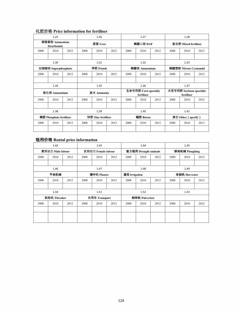
124
化肥价格 Price information for fertiliser
1.25 1.26 1.27 1.28
碳酸氢铵 Ammonium
bicarbonate 尿素 Urea 磷酸二铵 DAP 复合肥 Mixed fertiliser
2008 2010 2012 2008 2010 2012 2008 2010 2012 2008 2010 2012
1.30 1.31 1.32 1.33
过磷酸铵 Superphosphate 钾肥 Potash 硝酸铵 Ammonium 硝酸氛胺 Nitrate Cyanamid
2008 2010 2012 2008 2010 2012 2008 2010 2012 2008 2010 2012
1.34 1.35 1.36 1.37
氯化铵 Ammonium 氨水 Ammonia 玉米专用肥 Corn specialty
fertiliser
大豆专用肥 Soybean specialty
fertiliser
2008 2010 2012 2008 2010 2012 2008 2010 2012 2008 2010 2012
1.38 1.39 1.40 1.41
磷肥 Phosphate fertiliser 锌肥 Zinc fertiliser 硼肥 Boron 其它 Other(specify)
2008 2010 2012 2008 2010 2012 2008 2010 2012 2008 2010 2012
租用价格 Rental price information
1.42 1.43 1.44 1.45
男劳动力 Male labour 女劳动力 Female labour 畜力租用 Draught animals 耕地机械 Ploughing
2008 2010 2012 2008 2010 2012 2008 2010 2012 2008 2010 2012
1.46 1.47 1.48 1.49
平地机械 播种机 Planter 灌溉 Irrigation 收割机 Harvester
2008 2010 2012 2008 2010 2012 2008 2010 2012 2008 2010 2012
1.50 1.51 1.52 1.53
脱粒机 Thresher 农用车 Transport 粉碎机 Pulveriser
2008 2010 2012 2008 2010 2012 2008 2010 2012 2008 2010 2012
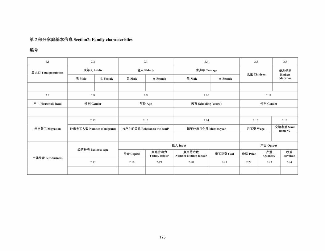
125
第 2 部分家庭基本信息 Section2: Family characteristics
编号
2.1 2.2 2.3 2.4 2.5 2.6
总人口 Total population
成年人 Adults 老人 Elderly 青少年 Teenage
儿童 Children
最高学历
Highest
education 男 Male 女 Female 男 Male 女 Female 男 Male 女 Female
2.7 2.8 2.9 2.10 2.11
户主 Household head 性别 Gender 年龄 Age 教育 Schooling (years ) 性别 Gender
外出务工 Migration
2.12 2.13 2.14 2.15 2.16
外出务工人数 Number of migrants 与户主的关系 Relation to the head* 每年外出几个月 Months/year 月工资 Wage 交给家里 Send
home %
个体经营 Self-business
经营种类 Business type
投入 Input 产出 Output
资金 Capital 家庭劳动力
Family labour
雇用劳力数
Number of hired labour 雇工花费 Cost 价格 Price
产量Quantity
收益Revenue
2.17 2.18 2.19 2.20 2.21 2.22 2.23 2.24
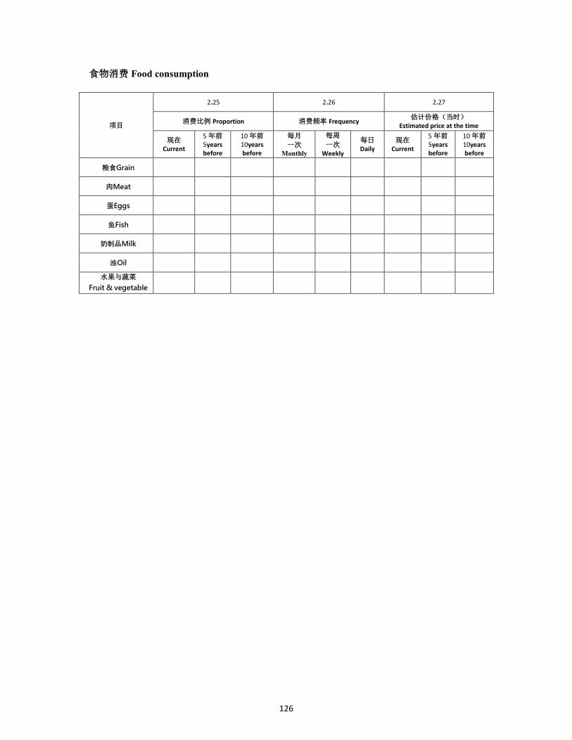
126
食物消费 Food consumption
项目
2.25 2.26 2.27
消费比例 Proportion 消费频率 Frequency 估计价格(当时)
Estimated price at the time
现在 Current
5 年前 5years before
10 年前 10years before
每月
一次
Monthly
每周
一次 Weekly
每日 Daily
现在 Current
5 年前 5years before
10 年前 10years before
粮食Grain
肉Meat
蛋Eggs
鱼Fish
奶制品Milk
油Oil
水果与蔬菜
Fruit & vegetable

127
第三部分:作物生产 Section 3:Cropping production
3.1 3.2 3.3 3.4 3.5 3.6 3.7 3.8 3.9
Crop code
作物代码
Crop area
种植面积
Plots
分为多少块
Land type
地块类型8
Yield
产量
Sold
出售了
Price
价格
Revenue
出售收入
Value 总收入
(产值)
Mu亩 块 Kg公斤 Kg公斤 Yuan 元 Yuan元 Yuan元
代码 Code:1.Wheat小麦 2. Maize 玉米 3. Beans 豆类 4. Potato 薯类 5. Oil 油料 6 Fruit水果 7. Vegetables大田蔬菜 8. Melons大田瓜类 9. Greenhouse vegetables大棚蔬菜 10.
Seedlings 苗木 11. Forage饲草料 12 Fertiliser grass 肥草料 13 Apple 苹果 14 Other其它(specify)
*3.41=Flat 平地 2= Hilly 低坡 3=Steep 陡坡 4=Valley 川地
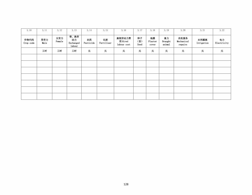
128
3.10 3.11 3.12 3.13 3.14 3.15 3.16 3.17 3.18 3.19 3.20 3.21 3.22
作物代码
Crop code
男劳力
Male
女劳力
Female
帮、换劳
动力
Exchanged
labour
农药
Pesticide
化肥
Fertiliser
雇佣劳动力费
用 Hired
labour cost
种子
(苗)
Seed
地膜
Plaster
cover
畜力
Draught
animal
农机服务
Mechanical
repairs
水利灌溉
Irrigation
电力
Electricity
工时 工时 工时 元 元 元 元 元 元 元 元 元
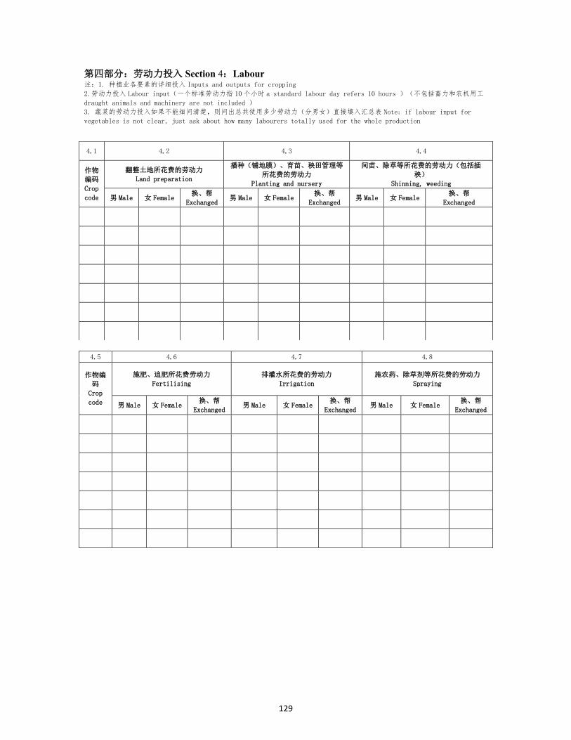
129
第四部分:劳动力投入 Section 4:Labour 注:1. 种植业各要素的详细投入 Inputs and outputs for cropping
2.劳动力投入 Labour input(一个标准劳动力指 10个小时 a standard labour day refers 10 hours )(不包括畜力和农机用工
draught animals and machinery are not included )
3. 蔬菜的劳动力投入如果不能细问清楚,则问出总共使用多少劳动力(分男女)直接填入汇总表 Note: if labour input for
vegetables is not clear, just ask about how many labourers totally used for the whole production
4.5 4.6 4.7 4.8
作物编
码
Crop
code
施肥、追肥所花费劳动力
Fertilising
排灌水所花费的劳动力
Irrigation
施农药、除草剂等所花费的劳动力
Spraying
男 Male 女 Female 换、帮
Exchanged 男 Male 女 Female
换、帮
Exchanged 男 Male 女 Female
换、帮
Exchanged
4.1 4.2 4.3 4.4
作物
编码
Crop
code
翻整土地所花费的劳动力
Land preparation
播种(铺地膜)、育苗、秧田管理等
所花费的劳动力
Planting and nursery
间苗、除草等所花费的劳动力(包括插
秧)
Shinning, weeding
男 Male 女 Female 换、帮
Exchanged 男 Male 女 Female
换、帮
Exchanged 男 Male 女 Female
换、帮
Exchanged
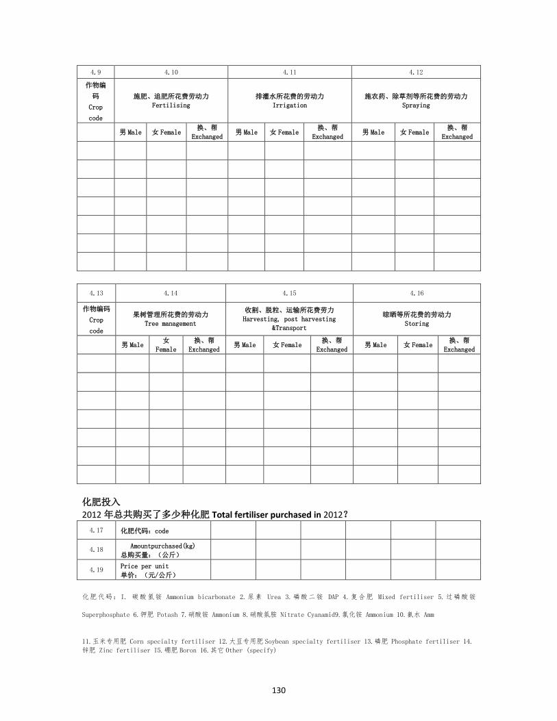
130
4.9 4.10 4.11 4.12
作物编
码
Crop
code
施肥、追肥所花费劳动力
Fertilising
排灌水所花费的劳动力
Irrigation
施农药、除草剂等所花费的劳动力
Spraying
男 Male 女 Female 换、帮
Exchanged 男 Male 女 Female
换、帮
Exchanged 男 Male 女 Female
换、帮
Exchanged
4.13 4.14 4.15 4.16
作物编码
Crop
code
果树管理所花费的劳动力
Tree management
收割、脱粒、运输所花费劳力
Harvesting, post harvesting
&Transport
晾晒等所花费的劳动力
Storing
男 Male 女
Female
换、帮
Exchanged 男 Male 女 Female
换、帮
Exchanged 男 Male 女 Female
换、帮
Exchanged
化肥投入
2012 年总共购买了多少种化肥 Total fertiliser purchased in 2012?
4.17 化肥代码:code
4.18 Amountpurchased(kg)
总购买量:(公斤)
4.19 Price per unit
单价:(元/公斤)
化肥代码:I. 碳酸氢铵 Ammonium bicarbonate 2.尿素 Urea 3.磷酸二铵 DAP 4.复合肥 Mixed fertiliser 5.过磷酸铵
Superphosphate 6.钾肥 Potash 7.硝酸铵 Ammonium 8.硝酸氛胺 Nitrate Cyanamid9.氯化铵 Ammonium 10.氨水 Amm
11.玉米专用肥 Corn specialty fertiliser 12.大豆专用肥 Soybean specialty fertiliser 13.磷肥 Phosphate fertiliser 14.
锌肥 Zinc fertiliser I5.硼肥 Boron 16.其它 Other (specify)
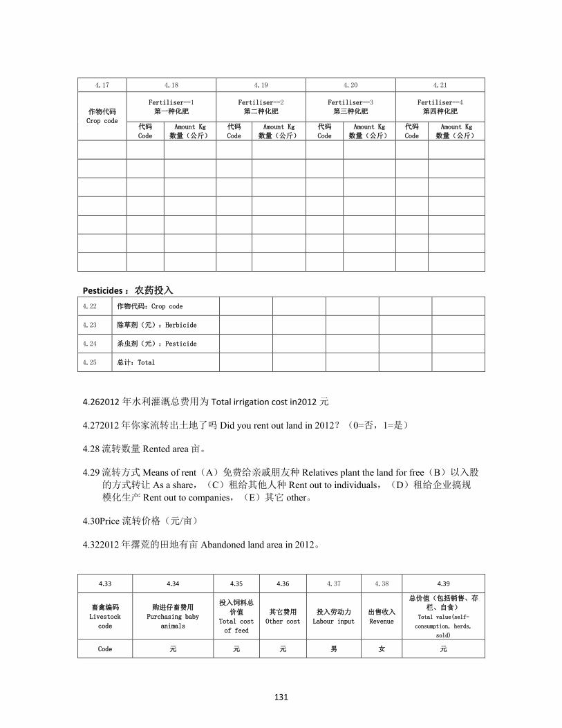
131
4.17 4.18 4.19 4.20 4.21
作物代码
Crop code
Fertiliser--1
第一种化肥
Fertiliser--2
第二种化肥
Fertiliser—3
第三种化肥
Fertiliser--4
第四种化肥
代码
Code
Amount Kg
数量(公斤)
代码
Code
Amount Kg
数量(公斤)
代码
Code
Amount Kg
数量(公斤)
代码
Code
Amount Kg
数量(公斤)
Pesticides :农药投入
4.22 作物代码:Crop code
4.23 除草剂(元):Herbicide
4.24 杀虫剂(元):Pesticide
4.25 总计:Total
4.262012 年水利灌溉总费用为 Total irrigation cost in2012 元
4.272012 年你家流转出土地了吗 Did you rent out land in 2012?(0=否,1=是)
4.28 流转数量 Rented area 亩。
4.29 流转方式 Means of rent(A)免费给亲戚朋友种 Relatives plant the land for free(B)以入股
的方式转让 As a share,(C)租给其他人种 Rent out to individuals,(D)租给企业搞规
模化生产 Rent out to companies,(E)其它 other。
4.30Price 流转价格(元/亩)
4.322012 年撂荒的田地有亩 Abandoned land area in 2012。
4.33 4.34 4.35 4.36 4.37 4.38 4.39
畜禽编码
Livestock
code
购进仔畜费用
Purchasing baby
animals
投入饲料总
价值
Total cost
of feed
其它费用
Other cost
投入劳动力
Labour input
出售收入
Revenue
总价值(包括销售、存
栏、自食)
Total value(self-
consumption, herds,
sold)
Code 元 元 元 男 女 元
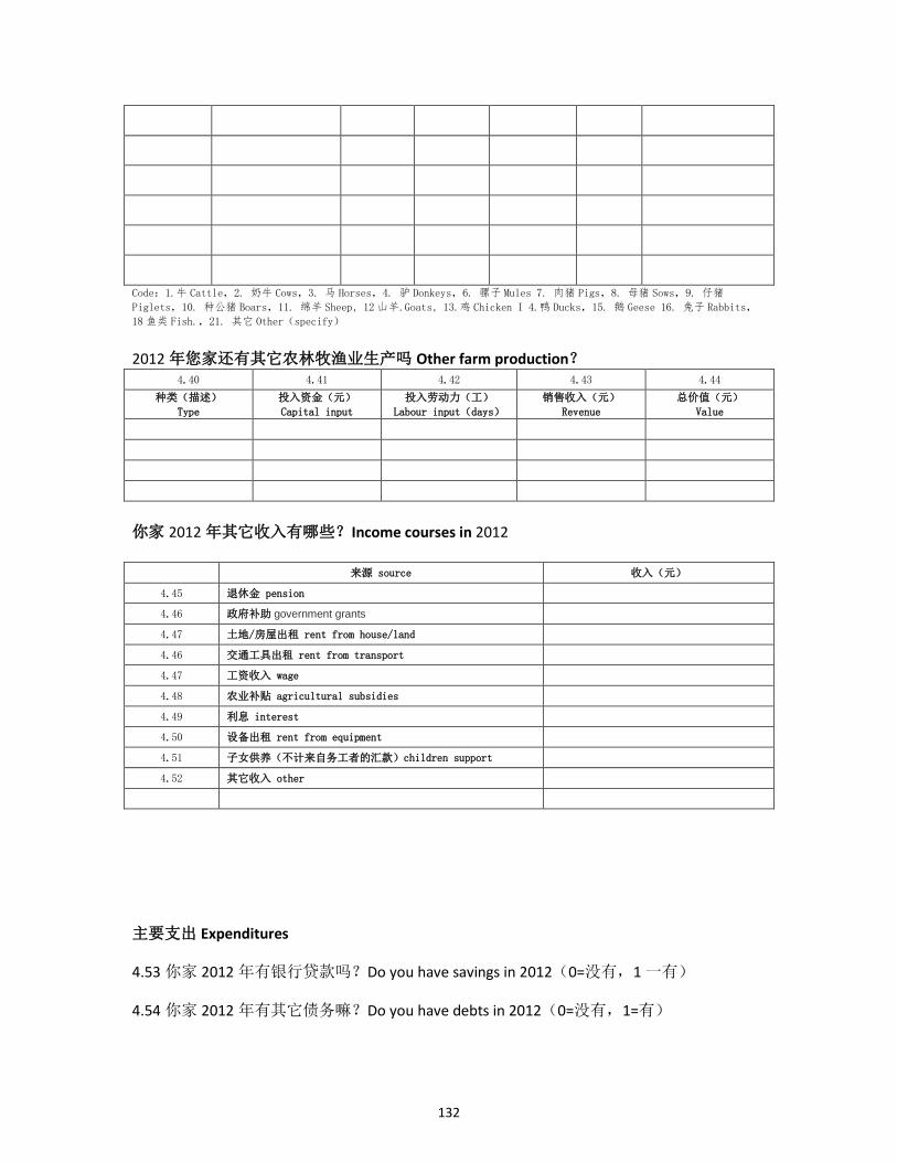
132
Code:1.牛 Cattle,2. 奶牛 Cows,3. 马 Horses,4. 驴 Donkeys,6. 骡子 Mules 7. 肉猪 Pigs,8. 母猪 Sows,9. 仔猪
Piglets,10. 种公猪 Boars,11. 绵羊 Sheep, 12山羊.Goats, 13.鸡 Chicken I 4.鸭 Ducks,15. 鹅 Geese 16. 兔子 Rabbits,
18鱼类 Fish.,21. 其它 Other(specify)
2012 年您家还有其它农林牧渔业生产吗 Other farm production? 4.40 4.41 4.42 4.43 4.44
种类(描述)
Type
投入资金(元)
Capital input
投入劳动力(工)
Labour input(days)
销售收入(元)
Revenue
总价值(元)
Value
你家 2012 年其它收入有哪些?Income courses in 2012
来源 source 收入(元)
4.45 退休金 pension
4.46 政府补助 government grants
4.47 土地/房屋出租 rent from house/land
4.46 交通工具出租 rent from transport
4.47 工资收入 wage
4.48 农业补贴 agricultural subsidies
4.49 利息 interest
4.50 设备出租 rent from equipment
4.51 子女供养(不计来自务工者的汇款)children support
4.52 其它收入 other
主要支出 Expenditures
4.53 你家 2012 年有银行贷款吗?Do you have savings in 2012(0=没有,1 一有)
4.54 你家 2012 年有其它债务嘛?Do you have debts in 2012(0=没有,1=有)
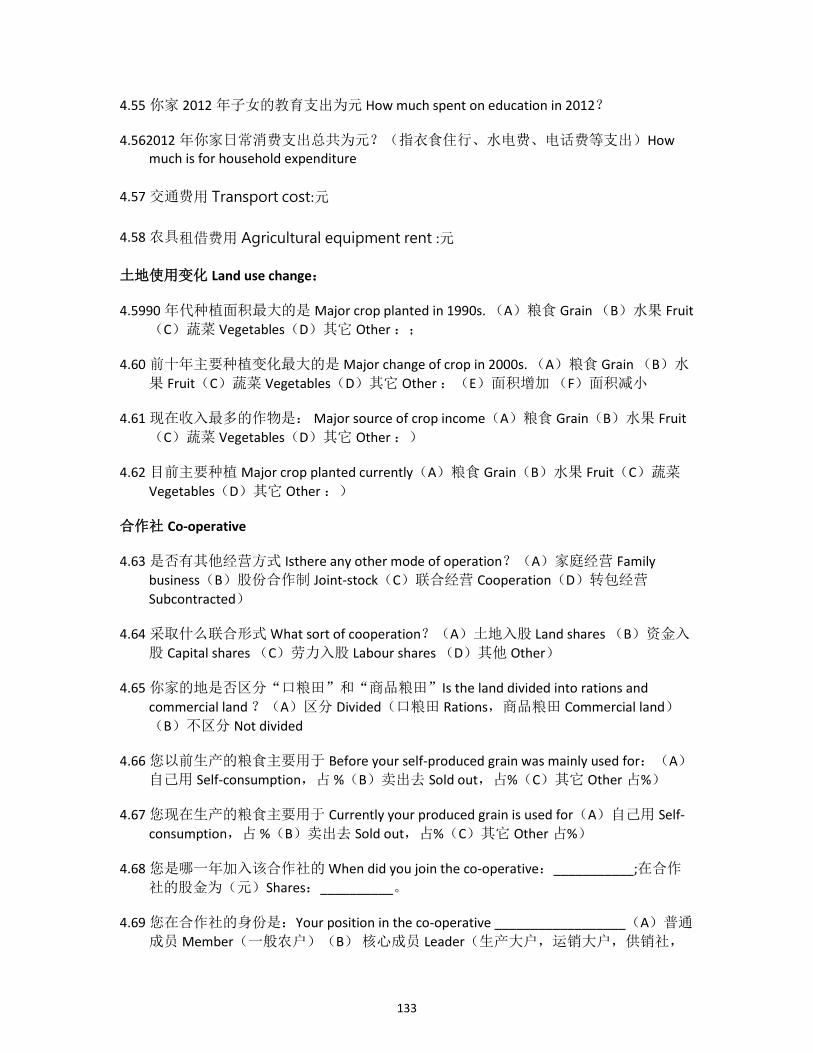
133
4.55 你家 2012 年子女的教育支出为元 How much spent on education in 2012?
4.562012 年你家日常消费支出总共为元?(指衣食住行、水电费、电话费等支出)How much is for household expenditure
4.57 交通费用 Transport cost:元
4.58 农具租借费用 Agricultural equipment rent :元
土地使用变化 Land use change:
4.5990 年代种植面积最大的是 Major crop planted in 1990s. (A)粮食 Grain (B)水果 Fruit
(C)蔬菜 Vegetables(D)其它 Other :;
4.60 前十年主要种植变化最大的是 Major change of crop in 2000s. (A)粮食 Grain (B)水
果 Fruit(C)蔬菜 Vegetables(D)其它 Other :(E)面积增加 (F)面积减小
4.61 现在收入最多的作物是: Major source of crop income(A)粮食 Grain(B)水果 Fruit
(C)蔬菜 Vegetables(D)其它 Other :)
4.62 目前主要种植 Major crop planted currently(A)粮食 Grain(B)水果 Fruit(C)蔬菜
Vegetables(D)其它 Other :)
合作社 Co-operative
4.63 是否有其他经营方式 Isthere any other mode of operation?(A)家庭经营 Family
business(B)股份合作制 Joint-stock(C)联合经营 Cooperation(D)转包经营
Subcontracted)
4.64 采取什么联合形式 What sort of cooperation?(A)土地入股 Land shares (B)资金入
股 Capital shares (C)劳力入股 Labour shares (D)其他 Other)
4.65 你家的地是否区分“口粮田”和“商品粮田”Is the land divided into rations and
commercial land ?(A)区分 Divided(口粮田 Rations,商品粮田 Commercial land)
(B)不区分 Not divided
4.66 您以前生产的粮食主要用于 Before your self-produced grain was mainly used for:(A)
自己用 Self-consumption,占 %(B)卖出去 Sold out,占%(C)其它 Other 占%)
4.67 您现在生产的粮食主要用于 Currently your produced grain is used for(A)自己用 Self-
consumption,占 %(B)卖出去 Sold out,占%(C)其它 Other 占%)
4.68 您是哪一年加入该合作社的 When did you join the co-operative:___________;在合作
社的股金为(元)Shares:__________。
4.69 您在合作社的身份是:Your position in the co-operative __________________(A)普通
成员 Member(一般农户)(B) 核心成员 Leader(生产大户,运销大户,供销社,
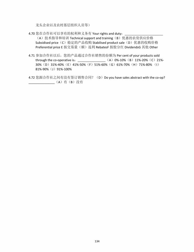
134
龙头企业以及农村基层组织人员等)
4.70 您在合作社可以享有的权利和义务有 Your rights and duty:______________________
(A)技术指导和培训 Technical support and training(B)优惠的农资供应价格
Subsidised price(C)稳定的产品收购 Stabilised product sale(D)优惠的收购价格
Preferential price E 按交易量(额)返利 RebatesF 按股分红 DividendsG 其他 Other
4.71 参加合作社以后,您的产品通过合作社销售的份额为 Per cent of your products sold
through the co-operative is:________________(A)0%-10%(B)11%-20%(C)21%-
30%(D)31%-40%(E)41%-50%(F)51%-60%(G)61%-70%(H)71%-80% (I)
81%-90%(J)91%-100%
4.72 您跟合作社之间有没有签订销售合同?(D)Do you have sales abstract with the co-op?
_______________(A)有(B)没有
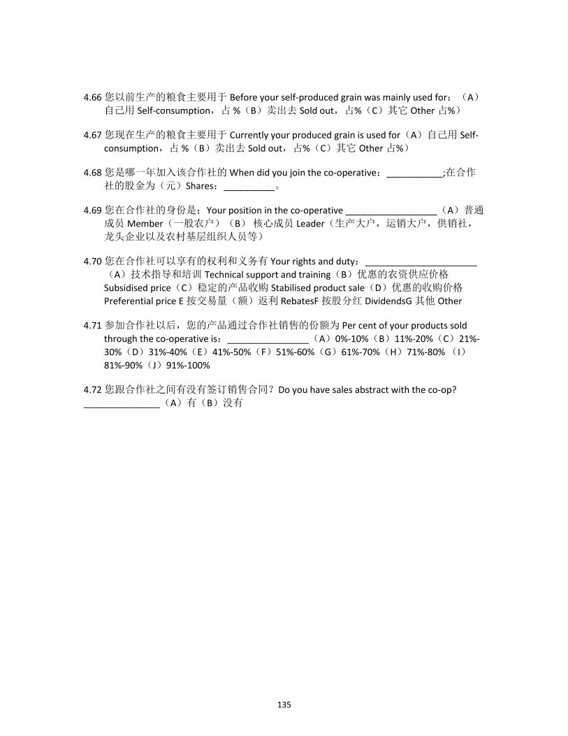
135
4.66 您以前生产的粮食主要用于 Before your self-produced grain was mainly used for:(A)
自己用 Self-consumption,占 %(B)卖出去 Sold out,占%(C)其它 Other 占%)
4.67 您现在生产的粮食主要用于 Currently your produced grain is used for(A)自己用 Self-
consumption,占 %(B)卖出去 Sold out,占%(C)其它 Other 占%)
4.68 您是哪一年加入该合作社的 When did you join the co-operative:___________;在合作
社的股金为(元)Shares:__________。
4.69 您在合作社的身份是:Your position in the co-operative __________________(A)普通
成员 Member(一般农户)(B) 核心成员 Leader(生产大户,运销大户,供销社,
龙头企业以及农村基层组织人员等)
4.70 您在合作社可以享有的权利和义务有 Your rights and duty:______________________
(A)技术指导和培训 Technical support and training(B)优惠的农资供应价格
Subsidised price(C)稳定的产品收购 Stabilised product sale(D)优惠的收购价格
Preferential price E 按交易量(额)返利 RebatesF 按股分红 DividendsG 其他 Other
4.71 参加合作社以后,您的产品通过合作社销售的份额为 Per cent of your products sold
through the co-operative is:________________(A)0%-10%(B)11%-20%(C)21%-
30%(D)31%-40%(E)41%-50%(F)51%-60%(G)61%-70%(H)71%-80% (I)
81%-90%(J)91%-100%
4.72 您跟合作社之间有没有签订销售合同?Do you have sales abstract with the co-op?
_______________(A)有(B)没有

136
农业生产性资产情况 Agricultural productive assets 4.732012 年你家拥有以下农具或役畜吗?*此处役畜非一般肉用畜禽
农具 编码 Code 水利设备 编码 Code 役畜等 编码 Code
手扶拖拉机 1 机井 Well 12 马 Horse 16
三轮车 Dray 2 水泵 Pumps 13 驴 Donkey 17
拖拉机 Tractor 3 水窖 14 骡 Mule 18
收割机Harvester
4 其它 Other 15 耕牛 Oxen 19
脱粒机Thresher
5 母猪 Pig 20
犁、耙等Plough
6 奶牛 Cow 21
家畜饲料加工机 7
家畜禽圈舍Pens
22
大棚Greenhouses
8
果园 Orchard 23
青贮窖 Silage 9
鱼塘 Fish Pond
24
畜棚 Shed 10
林地Woodland
25
其它农具 Other 11
其它 Other 26
生产资料编码 购置年份 购置价格(元) 生产资料编码
购置年份 购置价格(元)
非农资产情况 Non-agricultural asset 4.74 去年你家有下列家具或耐用消费品吗?
家具名称 编码 Code 家具名称 编码 Code 家具名称 编码 Code
电视机 TV 27 太阳能热水器 34 汽车 Car 38
VCD(DVD) 28 洗澡设备 35 摩托/电动车 39
电视卫星接收器 29 冰箱(冰柜)Refrigerator
36 音响 Sound 40
照相机 Camera 30 空调 Air
conditioning 37
电脑Computer
41
洗衣机 Washing machine
31 其它大件物品 Other
42
煤气灶 Gas stove
32
家具编码 购置年份 购置价格(元) 家具编码 购置年份 购置价格(元)
4.75 去年时你家有处住宅(House)?是否楼房? (0=否,1=是)购建年份?购建花费?
大于 3000 元的装修?维修年份?

137
第五部分劳动力的使用情况(每村调查五份左右即可,不是每户都填此表)
Activity
活动
5.1 5.2 5.3 5.4 5.5
Elderly 老人 Adults 青壮年 Teenage 青少年 Children
儿童 Hired labour 雇工
Ma le
男
Female
女
Ma le
男
Female
女
Ma le
男
Female
女
How
manyMale/Female
人数
Price
价格
Days
天数
What crop
哪种
作物
Land Preparation 整地
Ploughing 犁地
Planting 播种
Fertilising 施肥
Manuring 农家肥
Weeding 除草
Spraying 喷药
Irrigation 灌溉
Harvesting (grain)粮食收割
Tree management 果树管理
Tree harvesting 果园采摘
Post harvesting 打碾、晾晒
Transport 运输
Storing residue 储存
Cut & carry 割&运苜蓿
Feeding 喂家畜
Herding 放牧