Agilent 1290 Infinity 2D-LC Solution · The Agilent 1290 Infinity 2D-LC solution brings the power...
25
Agilent 1290 Infinity 2D-LC Solution A new flexible and user- friendly 2D-LC solution for the most complex samples Michael Frank Marketing Manager Analytical HPLC LPSD, Waldbronn, Germany April, 13 th 2012 1
Transcript of Agilent 1290 Infinity 2D-LC Solution · The Agilent 1290 Infinity 2D-LC solution brings the power...

Agilent 1290 Infinity
2D-LC Solution
A new flexible and user-
friendly 2D-LC solution for the
most complex samples
Michael Frank
Marketing Manager Analytical HPLC
LPSD, Waldbronn, Germany
April, 13th 2012
1

What is 2D-LC?
2
Peak capacities multiply for orthogonal separation mechanisms!
Two different modes:
Comprehensive 2D-LC (“LCxLC”)
Heart-cutting 2D-LC (“LC-LC”)
2D-LC: Injecting the efluent or a part of the effluent of one column to a second
column, ideally with orthogonal separation behavior.
Purpose: increase total separation power.

2D-LC - Difference between comprehensive 2D-LC
and heart-cutting 2D-LC
3
Comprehensive 2D-LC (LCxLC): The complete effluent of the first column will be injected to
the secnd column and will be analyized with very fast
gradients, a peak of the first dimension should be sampled
at least 3 to 4 times. The run time of the 2nd dimension
method matches the collection time of the 1st dimension
efluent. Finally, the peaks will be re-constructed. LC1
LC2
1st peak from
1st dimension
2nd peak from
1st dimension
3rd peak from
1st dimension
LC1
LC2

4
Only parts of the effluent of the first column – the
peaks eluted from the 1st dimension column - will
be injected to the second column.
Typically a peak from the first dimension will be
sampled as a whole and a gradient with a longer
run time than the collection time will be used. Also
longer columns with higher seperation efficiency are
being used in as 2nd dimension column.
Care must be taken if peaks are eluting from the
first dimension column when a gradient on the
second dimension is still running – this peak will be
lost.
Heart-cutting 2D-LC (LC-LC):
2D-LC - Difference between comprehensive 2D-LC
and heart-cutting 2D-LC
LC1
LC2

What is the Agilent 1290 Infinity 2D-LC solution?
• A new Agilent OpenLAB CDS ChemStation edition software add-on and new firmware features to allow easy set-up of 2D-LC methods using Agilent standard hardware.
• For comprehensive 2D-LC and heart-cutting 2D-LC
• Unique features like automatically shifted gradients or peak-triggered operation
• Highest focus on simplest but still highly flexible 2D-LC method set-up
• Highest flexibility on hardware set-up
– Different pumps, autosamplers and detectors supported, existing systems can be upgraded!
– Detectors at different positions (after 1st dimension column, after 2nd dim. column, at waste-line)
– Different valve set-up possibilities supported, one special new 2D-LC QuickChange valve head
– High performance data analysis by partner-solution
• Available June 2012
5

Data-Analysis
For heart-cutting 2D-LC by Agilent„s OpenLAB CDS ChemStation edition.
For comprehensive 2D-LC Agilent recommends:
GC Image LCxLC Edition Software from GC Image LLC.
Key features offered:
• Direct Agilent datafile import
• Peak identification, integration, annotation
• Comparative Analysis and Visualization
• Compound-libraries
• MS-data handling

Hardware – Module-flexibility
7
1. Dimension
2. Dimension
1290 Infinity
Binary Pump
1290 Infinity
Binary Pump
1290 Infinity
Autosampler or 1260
HiP Autosampler
Optional
1260/1290
Infinity
Detector
One or two
1290 Infinity
TCC
Optional
1260/1290
Infinity
Detector
1260/1290
Infinity
detector
1260 Infinity Binary
or Quaternary Pump
1260 Infinity
Capillary Pump 1260 Infinity
Autosampler
For 1st
dimension
chromatogram
and peak-
triggering
To monitor
waste-line
Almost any Agilent pump or autosampler in the 1st dimension!
Almost any detectors are supported!
A 1290 Infinity Binary Pump for the 2nd dimension is required.

Hardware – Module-flexibility
8
1. Dimension
2. Dimension
1290 Infinity
Binary Pump
1290 Infinity
Binary Pump
1290 Infinity Autosampler
or 1260 High Performance
Autosampler
Optional
1260/1290
Infinity
Detector
One or two
1290 Infinity
TCC
Optional
1260/1290
Infinity
Detector
1260/1290
Infinity Detector
1260 Infinity Binary
or Quaternary Pump
1260 Infinity
Capillary Pump 1260 Infinity
Autosampler
For 1st
dimension
chromatogram
and peak-
triggering
To monitor
waste-line
Most literatur known valve configurations based on 2pos-
10port or 2pos-6port valves are supported.

Hardware – Valves, uniqueness and flexibility
9
1. Dimension
2. Dimension
waste
Loop1
Loop2
2pos/4port-duo
New Agilent-only special 2D-LC-QucikChange valve.
Single valve with fully symmetric flow-paths and symmetric fill/flush-out
behavior. Only valve that allows countercurrent flush-out of both loops.

Advantages of the new Agilent 2D-LC QuickChange valve head
All flow paths are equal (no additional bridging loops)
Symmetric contercurrent fill/analyze direction of loops (reducing band-spread)
All in one valve (no synchronization, costs)
Loop1
Loop2
waste
2D-pump 2D-pump
1D-column
1D-column 1D-column
Fill direction Analyze direction
Valve
switching
1. 2.

Hardware – Valve-flexibility
11
1. Dimension
2. Dimension
waste
Loop1
Loop2
2pos/
10port
valve
Most other valve configurations for comprehensive and heart-cutting
2D-LC are supported as well. Easy transfer of existing 2D-LC methods!

Hardware – Valve-flexibility
12
1. Dimension
2. Dimension
waste
Loop1 Loop2
2x
2pos/6port
valves
Also dual valve-head configurations supported with automatic
synchronisation of valve-drives!

13
Dashboard: All modules in one dashboard can be relabled individually, e.g.
„BinPump-1st-Dim“
2D-LC Acquisition software An add-on to Agilent’s OpenLAB CDS ChemStation edition

Supported 2D-LC operation modes
14
Comprehensive LCxLC
Standard
or
Time-/Peak-triggered
Heart-cutting LC-LC
Time-triggered
or
Peak-triggered
level
1D chromatogram
2D sampling
2D gradient
level
complex/unknown samples: bio-
pharma, food, polymers....
Known samples/improving
confidence: pharma, meth.-dev..

15
• standard repeating with
start- and end-time
• constantly shifted %B2D
• constantly shifted %B2D
and shifted Δ%B2D
• Any combination
%B2D
Start 2D sampling End 2D sampling
%B1D
Time
%B2D
%B1D
Time
%B2D
%B1D
Time
%B2D
%B1D
Time
Comprehensive 2D-LC – gradient modes Special 2D-gradient modes to improve resolution

16
Time-segmenting in comprehensive 2D-LC Reducing cost!
1D Method run time
1D Gradient/
2D Gradients
Idle flow rate
2D Pump flow
rate
2D Pump flow rate
Solvent saving!!!
2D Time-segments
set in software idle
idle
idle
Time-triggered
Peak-triggered
Valve toggling
Increase life time!
%B (2D)
%B (1D)
F (2D)
1D
Me
tho
d p
ost-
run
tim
e
1D Chromatogram

17
Most easiest 2D-LC System Configuration “One screen for the entire system”
Define 1D / 2D pump
Define detector in the
second dimension
Define peak detector
(optional)
Select the valve(s) to
be used for 2D-LC
injection
Select a possible
valve / loop
configuration
Graphical representation of
the selected valve / loop
configuration:
• Flow path 1D & 2D
• Animated valve switching

18
Select the 2D-LC
mode: comprehensive
/ heart-cutting
Define the gradient of
the 2nd dimension
Define repetition of
2nd dimension
gradient (Modulation
time)
Show rollout of
gradient in the 2nd dim
over the runtime of
the 1st dimension
Define time
window(s) where the
selected 2DLC
mode is active
Most easiest set-up of complex 2D-LC methods 2D-LC specific parameters of the 2D-pump
Graphical editing of
gradient shift Access to standard
method UI of the
pump
Operation values,
warnings
Close-up of 2D-
gradient
Solvent & Flow-
Settings
Solvent consumption
calculation

19
Example: graphical editing of a gradient shift – in less than a minute! Replace editing of large timetables by a few mouse operations
1 Use context menu to enter the editing mode
3 Draw a straight line by dragging the mouse to a new %B value at a
specified runtime of the 1st dimension
2 Timetable entries are marked with circles
4 When releasing the mouse, a new TT entry is made and the gradient
rollout is automatically updated
6 Insert / Delete shift points (mouse cursor and context menu changes
near to a shift line)
5 Repeat step 3 + 4 with other TT entries
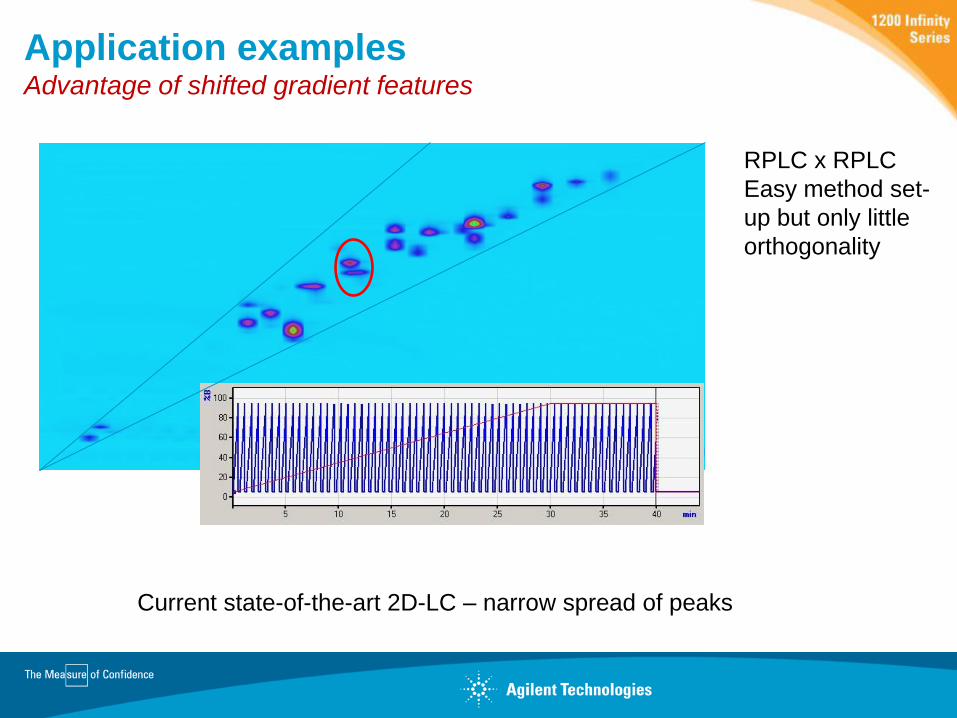
Application examples Advantage of shifted gradient features
Current state-of-the-art 2D-LC – narrow spread of peaks
RPLC x RPLC
Easy method set-
up but only little
orthogonality

Resolution optimized!
Application examples Advantage of shifted gradient features
Use of shifted
gradient feature
Imagine to program
this gradient manually!
With the Agilent 2D-
LC Acquisition
software a matter of
a minute!

Some Performance data Testmix of 20 compounds – 2D-Precision
0.00
0.50
1.00
1.50
2.00 2D-Retention Time Precision RSD (%)
0.00
1.00
2.00
3.00
2D-Peak Volume* Precision RSD (%)
1st Dimension: Eclipse Plus RRHD, C18, 150 x 2.1 mm,
1.8 µm. Flow rate: 0.1 mL/min. Gradient: 0 min 5% B – 30 min 95% B,
40min stop-time.
2nd Dimension: Eclipse Plus RRHD, Phenyl Hexyl, 50 x
3.0 mm, 1.8 µm Flow rate: 3 mL/min. Initial Gradient: 0 min - 5% B, 0.5 min -
15% B, 0.51 min - 5% B, 0.65 min - 5% B. Modulation-time 0.65 min
15 compounds <1% RSD,
all compounds <2% RSD
8 compounds <1% RSD,
16 compounds <2% RSD
*) not a peak area is measured but a three dimensional peak volume (intensity x 1D-time x 2D-time)!

Applications examples Polyphenols from food matrix
23
1
2
3
4
5
6
7
8 9
10
11
12 13 14
15
16
17 18 19
20 21 22
23
24
25 26
Compound
RT 1st dim
(min)
RT 2nd dim
(sec) Peak Volume
Esculin mean 9.75 18.58 177,383
s.d. nd 0.11 4,713
RSD (%) nd 0.57 2.7
Rutin mean 13.65 33.68 72,375
s.d. nd 0.07 853
RSD (%) nd 0.22 1.2
Coumaric acid mean 13.00 25.57 660,541
s.d. nd 0.13 13,037
RSD (%) nd 0.52 2.1
Reservatrol mean 18.85 26.65 1,122,219
s.d. nd 0.10 16,089
RSD (%) nd 0.37 1.4
Salicylic acid mean 19.50 18.53 211,092
s.d. nd 0.10 6,895
RSD (%) nd 0.51 3.3
Luteolin mean 19.50 32.70 695,601
s.d. nd 0.11 17,592
RSD (%) nd 0.33 2.5
7-Hydroxy-
Flavone mean 22.75 34.26 1,388,226
s.d. nd 0.10 17,195
RSD (%) nd 0.30 1.2
Pinoslyvin mean 24.70 18,85 1,588,654
s.d. nd 0.23 57,580
RSD (%) nd 1.24 3.6
Chrysin mean 27.30 27.42 808,916
s.d. nd 0.11 14,768
RSD (%) nd 0.39 1.8
Flavone mean 28.60 26.35 1,008,012
s.d. nd 0.13 20,911
RSD (%) nd 0.48 2.1
Peak volume:
all compounds <3.6% RSD
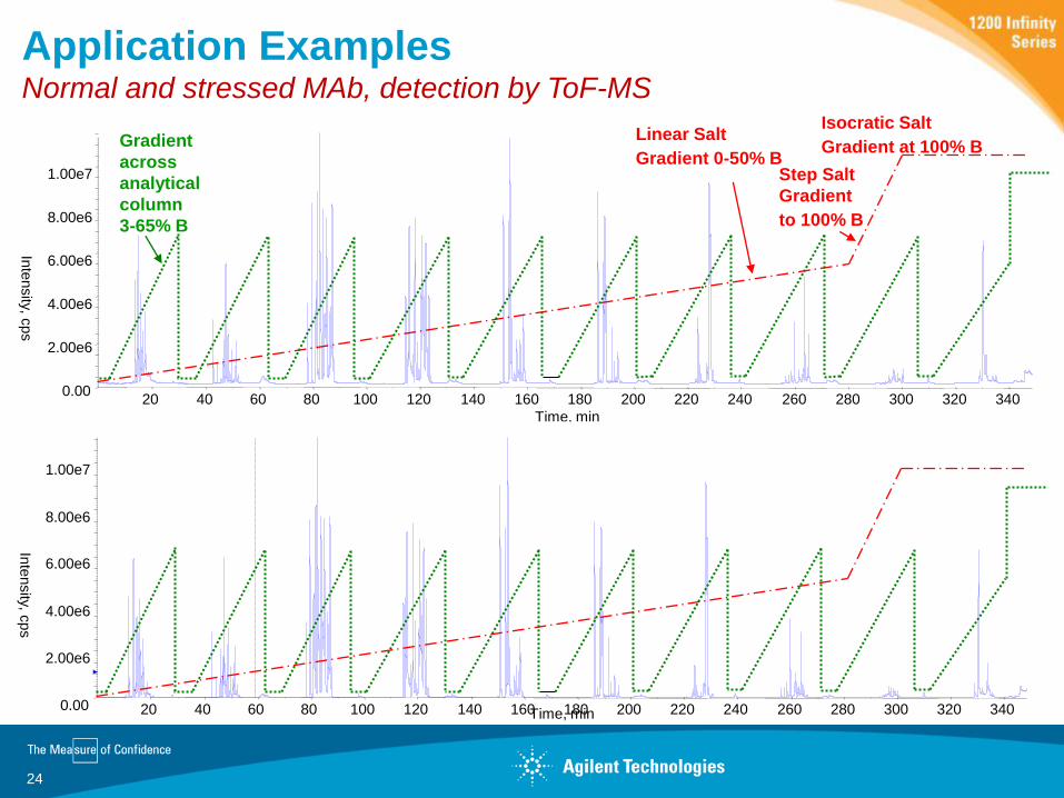
Application Examples Normal and stressed MAb, detection by ToF-MS
24
Inte
nsity
, cps
Gradient
across
analytical
column
3-65% B
20 40 60 80 100 120 140 160 180 200 220 240 260 280 300 320 340
Time, min
0.00
2.00e6
4.00e6
6.00e6
8.00e6
1.00e7
Linear Salt
Gradient 0-50% B Step Salt
Gradient
to 100% B
Isocratic Salt
Gradient at 100% B
20 40 60 80 100 120 140 160 180 200 220 240 260 280 300 320 340 Time, min 0.00
2.00e6
4.00e6
6.00e6
8.00e6
1.00e7
Inte
nsity, c
ps

Summary
25
The Agilent 1290 Infinity 2D-LC solution brings the power of two-dimensional LC-
separation to you at a never before experienced ease-of-use!
Highest separation power by 2D-LC combined with outstanding performance of the
1290 Infinity LC – the ideal tool for complex samples form biological origin, polymers,
food-extracs, and many more.
Innovative new hardware and software features for ease-of-use, reduced operation
costs and highest performance.
Upgradability or re-use of existing Agilent LC equipment.


![Agilent 1290 Infinity LC 월등히 강력해진 성능 · 1290 Infinity LC 액체 이송 시스템의 뛰어난 기능과 차세대 ... 510 505 &' O[ Ï] 495 8.5 9.0 ... • 램프](https://static.fdocuments.net/doc/165x107/5b8a66067f8b9aa81a8e79ff/agilent-1290-infinity-lc-1290-infinity-lc-.jpg)