Aggregation and the PPP Puzzle in a StickyPrice Model�

Carlos CarvalhoFederal Reserve Bank of New York

Fernanda NechioPrinceton University

May 2009

�The views expressed in this presentation are those of the authors and do not necessarily re�ect theposition of the Federal Reserve Bank of New York or the Federal Reserve System.

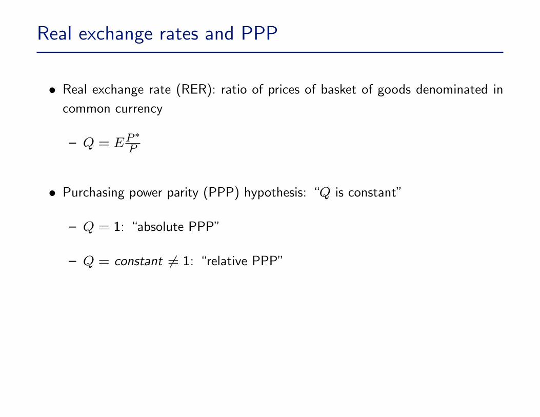
Real exchange rates and PPP

� Real exchange rate (RER): ratio of prices of basket of goods denominated incommon currency

� Q = EP�P

� Purchasing power parity (PPP) hypothesis: �Q is constant�

� Q = 1: �absolute PPP�

� Q = constant 6= 1: �relative PPP�

US Dollars / "French Franc-Euro"

0.4

0.6

0.8

1

1.2

1.4

1.6Ja

n-83

Jan-

84

Jan-

85

Jan-

86

Jan-

87

Jan-

88

Jan-

89

Jan-

90

Jan-

91

Jan-

92

Jan-

93

Jan-

94

Jan-

95

Jan-

96

Jan-

97

Jan-

98

Jan-

99

Jan-

00

Jan-

01

Jan-

02

Jan-

03

Jan-

04

Jan-

05

Jan-

06

Jan-

07

Jan-

08

Jan-

09

0.4

0.6

0.8

1

1.2

1.4

1.6

FX (left axis) RER (left axis) Price Ratio (right axis)

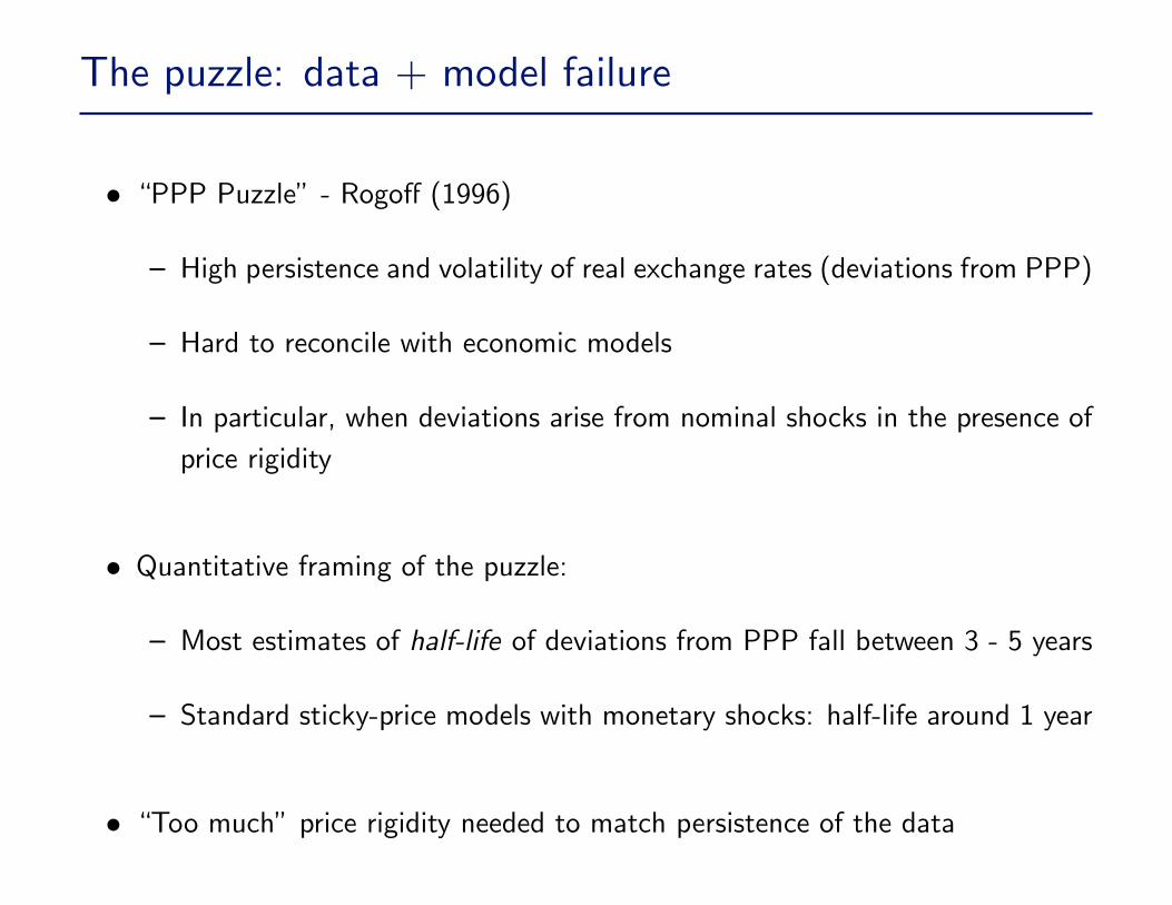
The puzzle: data + model failure

� �PPP Puzzle� - Rogo¤ (1996)

� High persistence and volatility of real exchange rates (deviations from PPP)

� Hard to reconcile with economic models

� In particular, when deviations arise from nominal shocks in the presence ofprice rigidity

� Quantitative framing of the puzzle:

� Most estimates of half-life of deviations from PPP fall between 3 - 5 years

� Standard sticky-price models with monetary shocks: half-life around 1 year

� �Too much�price rigidity needed to match persistence of the data

Our paper

� Build on ample evidence of heterogeneity in frequency of price adjustment (Bilsand Klenow 2004 and others)

� Average degree of price rigidity not the relevant statistic for aggregatedynamics (Carvalho 2006)

� Potential source of heterogeneity in dynamics of sectoral real exchange rates

� Multi-sector, two-country, sticky-price model:

� Heterogeneity in frequency of price changes

� Price discrimination and local currency pricing

) Heterogeneous sectoral real exchange rates

Summary of the model - K sectors

Consumers Consumers*

Home Foreign

FinalGoods

FinalGoods*

IntermediateGoods

IntermediateGoods*

Sector 1 ... Sector KSector k ...YH,k,j

Y*H,k,j

Sector 1 ... Sector KSector k ...YF,k,j

Y*F,k,j

C

L

C*

L*

Y Y*

YH,k,j Y*H,k,j YF,k,j Y*

F,k,j

Summary of the model - 1 sector

Consumers Consumers*

Home Foreign

FinalGoods

FinalGoods*

IntermediateGoods

IntermediateGoods*

C

L

C*

L*

Y Y*

YH,j Y*H,j YF,j Y*

F,j

Summary of core quantitative results

� Quantitative model

� Discipline our argument: distribution of price stickiness chosen to matchmicro data

� Average frequency of price changes implies average spells of 4.4 months

� Half-life of deviations from PPP in heterogeneous economy: 3.8 years

� Half-life of deviations from PPP in homogeneous economy: 1.2 years

Core results: intuition I

� Sectors with more stickiness are disproportionally important for aggregate dy-namics

� Extreme case: 1 �exible- and 1 sticky-price sector, no pricing complementarities

� Aggregate RER dynamics driven only by sticky-price sector

� Mathematically: measures of persistence (and volatility) are convex in thefrequency of price changes

Core results: intuition II

� E¤ects even stronger in the presence of pricing complementarities!

� Not-so-extreme version of �responders vs non-responders�of Haltiwanger andWaldman (1991)

� Bottom line in terms of persistence:

� heterogeneous economy � homogeneous economy with more price sticki-ness than what�s implied by average frequency of price changes

The model

� Two countries, Home and Foreign, with identical, in�nitely lived consumers

� Commodities are labor, a consumption good and a continuum of intermediategoods

� Consumer supplies labor, invests in complete set of state-contingent assets, andconsumes non-traded �nal good

� Competitive �nal good producers bundle intermediate goods; �exible prices

� Monopolistically competitive intermediate goods producers:

� Price discriminate, setting prices in local currency

� Sticky prices; adjustment frequency varies across sectors

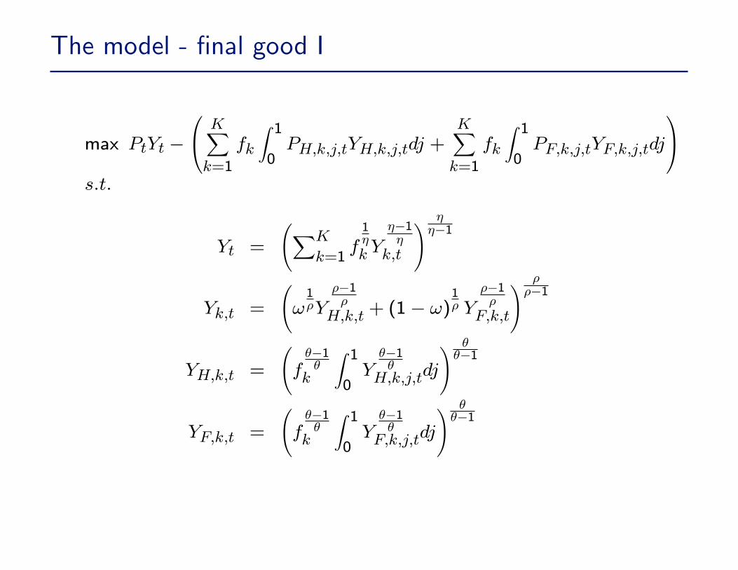
The model - �nal good I

max PtYt �

0@ KXk=1

fk

Z 10PH;k;j;tYH;k;j;tdj +

KXk=1

fk

Z 10PF;k;j;tYF;k;j;tdj

1As:t:

Yt =

XK

k=1f1�k Y

��1�

k;t

! ���1

Yk;t =

!1�Y

��1�

H;k;t + (1� !)1� Y

��1�

F;k;t

! ���1

YH;k;t =

f��1�

k

Z 10Y��1�

H;k;j;tdj

! ���1

YF;k;t =

f��1�

k

Z 10Y��1�

F;k;j;tdj

! ���1

The model - �nal good II

� Demands

YH;k;j;t = !

PH;k;j;t

PH;k;t

!�� PH;k;tPk;t

!�� Pk;tPt

!��Yt

YF;k;j;t = (1� !) PF;k;j;t

PF;k;t

!�� PF;k;tPk;t

!�� Pk;tPt

!��Yt

� Price Indices:

Pt =�XK

k=1fkP

1��k;t

� 11��

Pk;t =�!P

1��H;k;t + (1� !)P

1��F;k;t

� 11��

PH;k;t =

Z 10P 1��H;k;j;tdj

! 11��

PF;k;t =

Z 10P 1��F;k;j;tdj

! 11��

The model - intermediate �rms I

� Intermediate �rms:

� divided into sectors that di¤er in the frequency of price changes

� Calvo (1983) pricing: �k = frequency of price changes in sector k

� indexed by country, sector (k 2 K), and by j 2 [0; 1]

� sectoral weights fk

� produce di¤erentiated varieties using labor

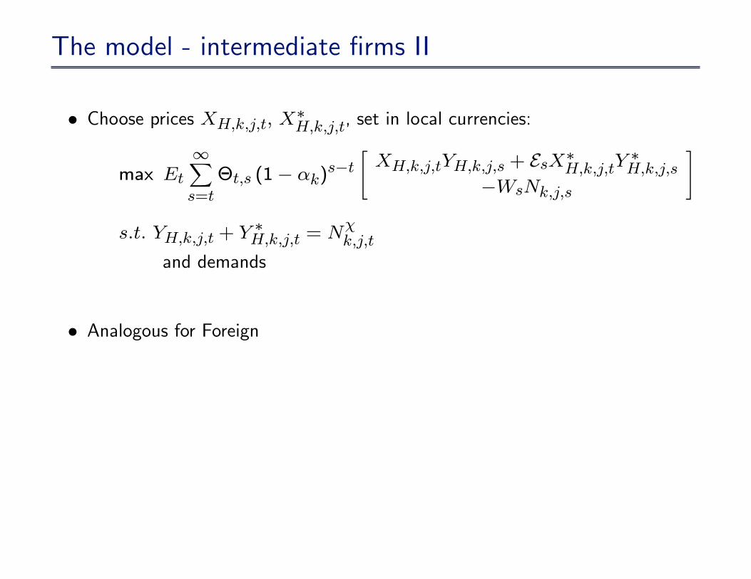
The model - intermediate �rms II

� Choose prices XH;k;j;t; X�H;k;j;t, set in local currencies:

max Et

1Xs=t

�t;s (1� �k)s�t"XH;k;j;tYH;k;j;s + EsX�H;k;j;tY

�H;k;j;s

�WsNk;j;s

#

s:t: YH;k;j;t + Y�H;k;j;t = N

�k;j;t

and demands

� Analogous for Foreign

The model - aggregate and sectoral RERs

� Aggregate:

Qt �EtP �tPt

� Sectoral:

Qk;t �EtP �k;tPk;t

Closing the model

� Speci�cations for monetary policy that ensure existence and uniqueness of REequilibrium

� Equilibrium: optimality and market clearing conditions

� Solution: loglinearization around zero in�ation steady-state

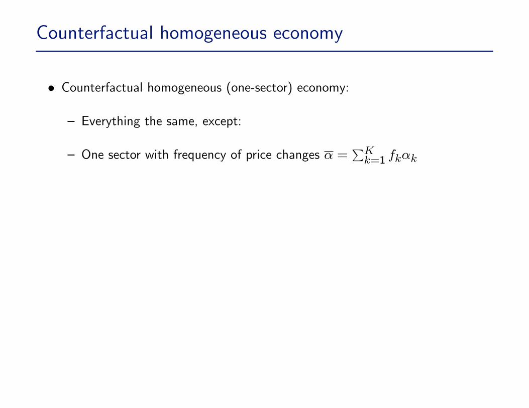
Counterfactual homogeneous economy

� Counterfactual homogeneous (one-sector) economy:

� Everything the same, except:

� One sector with frequency of price changes � =PKk=1 fk�k

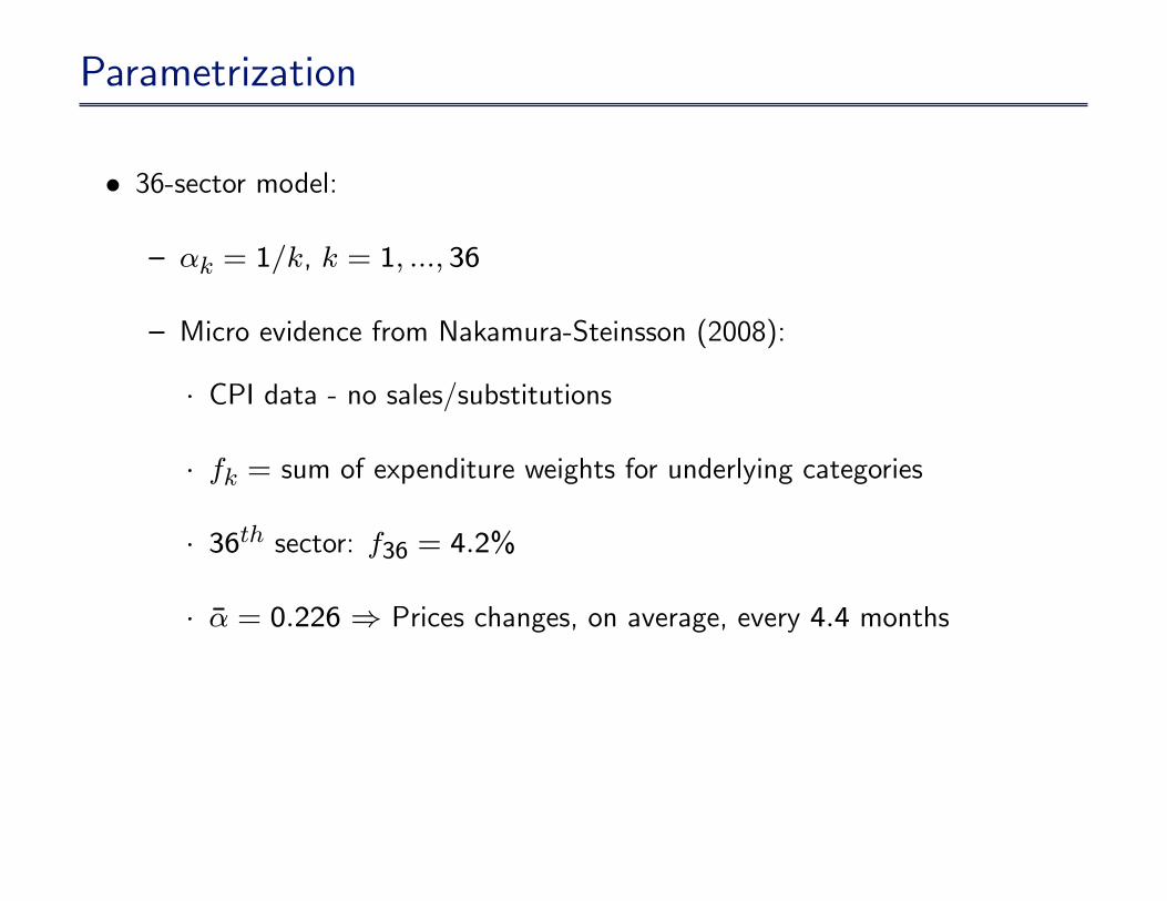
Parametrization

� 36-sector model:

� �k = 1=k, k = 1; :::; 36

� Micro evidence from Nakamura-Steinsson (2008):

� CPI data - no sales/substitutions

� fk = sum of expenditure weights for underlying categories

� 36th sector: f36 = 4:2%

� �� = 0:226 ) Prices changes, on average, every 4:4 months

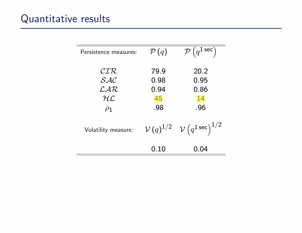
Quantitative results

Persistence measures: P (q) P�q1 sec

�CIR 79:9 20:2SAC 0:98 0:95LAR 0:94 0:86HL 45 14�1 :98 :96

Volatility measure: V (q)1=2 V�q1 sec

�1=20:10 0:04

Using our structural model - extras

� We provide structural interpretation to the (reduced-form) empirical literatureon heterogeneity, aggregation and PPP

� �PPP Strikes Back/Aggregation Bias�debate between Imbs et al. (2005),and Chen and Engel (2005) / Crucini and Shintani (2008)

� Study persistence in the cross-section of sectoral exchange rates ; touch basewith Kehoe and Midrigan (2008) (this is work in progress)

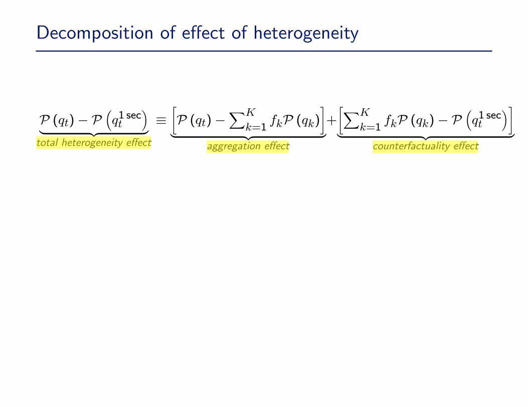
Decomposition of e¤ect of heterogeneity

P (qt)� P�q1 sect

�| {z }total heterogeneity e¤ect

��P (qt)�

XK

k=1fkP (qk)

�| {z }

aggregation e¤ect

+�XK

k=1fkP (qk)� P

�q1 sect

��| {z }

counterfactuality e¤ect

Applying decomposition

"Eurostatdata

#Data Panel, agg. Panel, sect. Panel, sect.

Estim. method Fixed E¤ects OLS MGP (q) 1

K

PP (qk) P�q1 sec

�Persist. meas.:

CIR 64:39 59:48 33:19SAC 0:98 0:97 0:97LAR 0:97 0:94 0:95HL 46 43:16 26

"Simulateddata

#Economy Heterog. Heterog. One-sectorData Single, agg. Panel, sect Single, agg.

Estim. method OLS OLS OLSP (q) 1

K

PP (qk) P�q1 sec

�Persist. meas.:

CIR 73:4 60:8 36:9SAC 0:98 0:97 0:97LAR 0:96 0:89 0:87HL 43:1 31:6 21:8

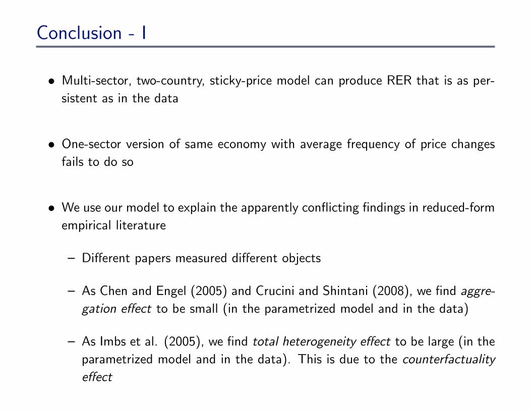
Conclusion - I

� Multi-sector, two-country, sticky-price model can produce RER that is as per-sistent as in the data

� One-sector version of same economy with average frequency of price changesfails to do so

� We use our model to explain the apparently con�icting �ndings in reduced-formempirical literature

� Di¤erent papers measured di¤erent objects

� As Chen and Engel (2005) and Crucini and Shintani (2008), we �nd aggre-gation e¤ect to be small (in the parametrized model and in the data)

� As Imbs et al. (2005), we �nd total heterogeneity e¤ect to be large (in theparametrized model and in the data). This is due to the counterfactualitye¤ect

Conclusion - II

� What matters for understanding the gap between data and standard one-sectormodels is total heterogeneity e¤ect

� Heterogeneity in price stickiness goes a long way towards solving the PPPpuzzle

� Such type of heterogeneity known to matter for policy:

� In �closed economies�: Aoki (2001), Benigno (2004), Eusepi, Hobjn andTambalotti (2008), Berriel and Sinigaglia (2008)

� In open economies: ?