Agenda: Quantum Mechanics Postulates & Consequences

Agenda: Quantum Mechanics Postulates & Consequences

• Quantum Postulates (Claims)

Correspondence principle

The quantum probability density flow

Eigen and expectation values

Overlap integrals, Dirac notation

Compatible and incompatible measurements

Time dependence

• Copenhagen interpretation of QM

System-detector interactions

Paradoxes, entanglement

Alternative trial interpretations

• Case study: Exploring electron spin polarization

• Stern-Gerlach polarimeters,

• Electron spinor states

W. Udo Schröder, 2020

Post

ulat

es

Prob

1

Overlap Integral and Expectation Value


Post

ulat

es

Prob

2

Overlap integral of 2 normalized functions measures their similarity (example: spatial symmetry). Maximally dissimilar (orthogonal) functions have zero overlap.

2* 2

2

: ( ...) ( ,...)

1 0

1

: 0 ; and

G definitions for any no

r

rmalized system wfs

x x dx wit

eneral

Ove

n

h

Rang o

rla

g

p

are to eacoe ortho l h thea

−

= = =

=

ˆ ˆ, .

1

:

ˆ ˆ

a

a a a a a a

Exception EigIn general A is dissimilar to A

w

enfunctio

Aith a a

ns

A a

−

= → = =

*

** *

:

ˆ ˆ( ...) ( ,...)

ˆ ˆ ˆ( ...) ( ,...) ( ,...) (

ˆ

...)

Necessary requirements for operator corresponding to observable A

A x real valA x dx

A A x x dx x A x dx

ue

A

−

− −

= =

= =

ExpectationValue

*ˆ ˆ ˆ ˆ ˆ ˆ ˆ ˆ

D

A

irac not o

A A A

a

A A A A

ti n

= → = = = =

Dirac Notation for Overlap Integrals


Post

ulat

es

Prob

3

*, ;

.etc

→ = =

+ = +

Per definition (integral):Anti-linear

2

: 0 1; 0 and

G

r

eneral definitions for any normalized system wfs

Ra are orthogonal to each othnge e =

( ) ˆ

1

"

ˆ ˆ

: " ker

a a a

a a

a

a a

aa

a

Eigenfunction for any observabi le operator A

with a a

l

s

A A

e

a

Kronec dSpecia f ature

ex st

elta

=

=

= → =

* †

( ...)

( ...) ( )

wf x state vector in Hilbert space

wf x vector in adjunct conjugate

H;

H

Dirac Notation for usein overlap integrals:

" " , " "bket ra

Expansion in Dirac Notation


Post

ulat

es

Prob

4

( )

( )

ˆ ˆ:

ˆ ˆ

Matrix element of A A square matrix A

A A numeric values

= =

a orthonormalized set of wfs =: a a aaSpecial feature =

" " aaKronecker delta

( )

2

: ...

, ( )1

a aa

aa

ac Norm

G a

alizati

eneric w ve p

on for discrete

c

E

k

V

a e

a

t c

c

=

=

Also solution to TDSE:(Superposition Theorem

Expansion Theorem)

( ) ˆ

ˆ ˆ 1a a a a a a

a for any observable operator A

with a a a

Wave functions are solutions to TDSE

E exiig c senfun tions

A A

t

= → = = Because only eigen values are measured

Instant Quiz


Post

ulat

es

Prob

5

ˆˆa a a

a a aa

for operatorConsider eigenfunction A with a

Show t

s A

hat

=

=

ˆ ˆa a a a aUse A Aa and a with a = =

Agenda: Quantum Mechanics Postulates & Consequences

• Quantum Postulates (Claims)

Correspondence principle

The quantum probability density flow

Eigen and expectation values

Overlap integrals, Dirac notation

Compatible and incompatible measurements

Time dependence

• Copenhagen interpretation of QM

System-detector interactions

Paradoxes, entanglement

Alternative trial interpretations

• Case study: Exploring electron spin polarization

• Stern-Gerlach polarimeters,

• Electron spinor states


Post

ulat

es

Prob

8

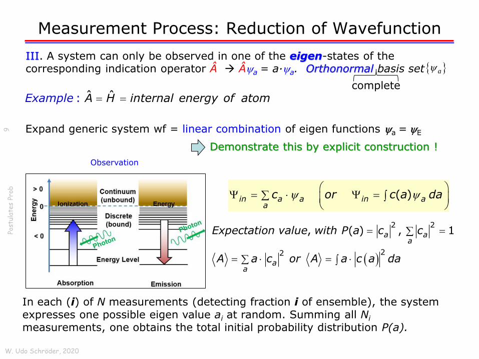
Measurement Process: Reduction of Wavefunction


Post

ulat

es

Prob

9

III. A system can only be observed in one of the eigen-states of the corresponding indication operator Â → Âa = a·a. Orthonormal basis set a

ˆ: ˆA H internal energy of atomExample = =

( )in a a in aa

c or c a da

= =

Expand generic system wf = linear combination of eigen functions a = E

( )

2 2

22

, ( ) , 1a aa

aa

Expectation value with P a c c

A a c or A a c a da

= =

= =

In each (i) of N measurements (detecting fraction i of ensemble), the system expresses one possible eigen value ai at random. Summing all Ni

measurements, one obtains the total initial probability distribution P(a).

Observation

Demonstrate this by explicit construction !

complete

Measurement Process: Reduction of Wavefunction


Post

ulat

es

Prob

10

III. A system can only be observed in one of the eigen-states of the corresponding indication operator Â → Âa = a·a. Orthonormal basis set a

After one measurement, each sub-part (i) of system ensemble populates one distinct eigen state: Probability Pfin(a=ai) = |cai|

2.

2 2ˆ ˆ

" "

a i a i ai i i

fin ai i

A a A a

System prepared as

= =

→

Separation of sub systems according to measured values ai permits repetition of the same measurement on components i.

Result: Selected system remains in the same normalized eigen state: Pfin(ai) = 1.

Observation

in a aa

c =

( )2

in a a fin i aia

c P a c

= →→

Measurement

in collapses into incoherent sum of components !(ongoing research)

Ideal Expectation: System-Apparatus Int.

Debate from the start of QM: Measure dynamical variable W (observable) of system S with an experimental apparatus A.


Post

ulat

es

Prob

11

S

A

Info in state vector/wave function S

Projected with some W sensitivity projector P

Argument assumes discrete eigen spectra

) )

ˆ ˆSystem eigen states of : ;n ;n

ˆ ˆApparatus : eigen states of A : A ;m ;m

indicator variable(e.g. position of needle)

m,n auxiliary qu.#s

W W =

=

=

)

)

; ;

( ) ; ;

S A states LinComb of n m

Assume pure initialsimple n m

=

( ) ( ) ( )

( ) ) )

,..., ,...

, ,

ˆ ˆ ˆ:

" "

,,ˆ ; ; ; ;

,,n m

Time t after measurement unitary operator t p t t

entanglement because interaction S with A mixes states

nnt n m p n m

mm

P = P P

P = →

correlation → , to make A proper indicator

Measurement : System-Apparatus

Transition amplitude p. Coherent superposition of A states, emphasis on eigen value (by construction of apparatus).

Macroscopic state of system at time t, after measurement:


Post

ulat

es

Prob

12

( ) ( ) ( )( ),

ˆ ; , , ;t

n

S t n p n n n

= P = →

S

A

) ( ) )

), ,

ˆ ;

,,;

,,

t

n m

t m

nnp m

m

A

m

= P

= →

Macroscopic state of measurement apparatus at time t, after measurement:

Macroscopic state of system: different from initial state, no longer Weigenstate, but a coherent superposition → subsequent measurements of the same observable on the same event would produce different outcomes →

Not consistent with postulated “collapse of the wave function” attributed to measurement process. → future t solutions??

Density matrix approach more appropriate?QM prep and measurement

Repeated Measurements

N repeated measurements of observable A on many identically prepared

microscopic systems, with the same detector. Accumulate events with ai.


Post

ulat

es

Prob

13

( )ˆ ˆ: a aObservable values of A eigen values of A A a

Repeated measurements on events with same a return the same a

= =

Correspondence Principle: For any observable A,

there is a quantal operator projecting mean A & variance

( ) ( )

( )

( )( )

*

22 2

21 2

2

2

ˆ ˆ: , ,

ˆ ˆ

( ): 2 exp

2

all space q

A

A

A

A A dq q t A q t and

Variance A A

A AdP Aprobability distribution

dA

−

= =

= −

− → = −

( ) ( )1

( ): # ,iP a of events i with a a a a a dP a da normalizedN

= + →

( ) ( ) ( )0 0 0" " : , , ,aCollapse of wave function q t t q t t q t →

Instant Quiz

Copenhagen interpretation: quantum-statistics (not thermal!)


Post

ulat

es

Prob

14

( )

( ) ( )

2

A with a , set of eigen functions ,

, , ;

Probability ( )

a

a a aa

a a a

complete orthonormal x t

system stae te wave function x t c x t c

c P a c

Pur

→ =

= → =

0 1 1 0 1 0 2 0

0E 1E 1E 0E 1E 0E 2E 0E

Preparation of many instances of same quantum state

Measurement

Data Analysis

?? ??Deduce mean energy E and wave function = =

Compatible and Incompatible Measurements: HUR


Post

ulat

es

Prob

17

IV. A series of successive ensemble measurements of observables A, B →

probability distribution P(A), mean and variance are given by

A B

Heisenberg Uncertainty Relation for sequ

Standard uncer

e t

taintie

l

s a

n ia

nd

( )2 2

21

ˆ ˆ ˆ ˆ... ( ) ( )ˆ ˆ ˆˆi i baAB dq q B q BA Aa d BAn

= = −

ˆ

,

( )i

In general wave function is not eigen function of observable A

qA

→ ˆ( ) ( ) (ˆ ˆ )i i iq changes q B qA A → →

ˆ ( )

ˆ ( )

i

i

B q

B q

→ ˆ ˆ( ) ( ) ( )ˆi i iq B change q qAs B → →

:

ˆ ( )

,

iq

In general measuremen e

A

ts of A and B ar incompatible

→

ˆ ˆ ˆˆ ˆˆ 0

0,C

eommutator A

B aB A

m

A and com

t

p t

A and

i

B no co pat l

blB B

eA

ib

= −

=

1 ˆ ˆ, 22

A B A B

Notation

Post

ulat

es

Prob


18

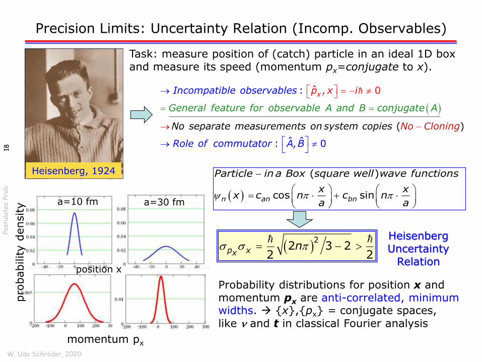
Precision Limits: Uncertainty Relation (Incomp. Observables)

( )2

2 3 22 2

p xxn = −

Heisenberg Uncertainty

Relation

Heisenberg, 1924

a=10 fm a=30 fm

Probability distributions for position x and momentum px are anti-correlated, minimum widths. → {x},{px} = conjugate spaces, like n and t in classical Fourier analysis

Task: measure position of (catch) particle in an ideal 1D box and measure its speed (momentum px=conjugate to x).

position x

momentum px

pro

bability d

ensity

( )

( )

cos sinn an bn

Particle in a Box square well wave functions

x xx c n c n

a a

−

= +

( )

:

ˆ ˆ: , 0

(

ˆ

)

, 0x

General feature for observable A and B conjugat

No separate meas

m

urements o

b

n sy

e

st

t

e

A

m

l

c

s

o

x

p

r

i

c

e

n

s

I omp o

No

e

C

a

l

i

o

l

n

a

i

e

n

o

g

b bs rv

Role of com utat A

p i

e

B

→

=

= −

→

→

=

−

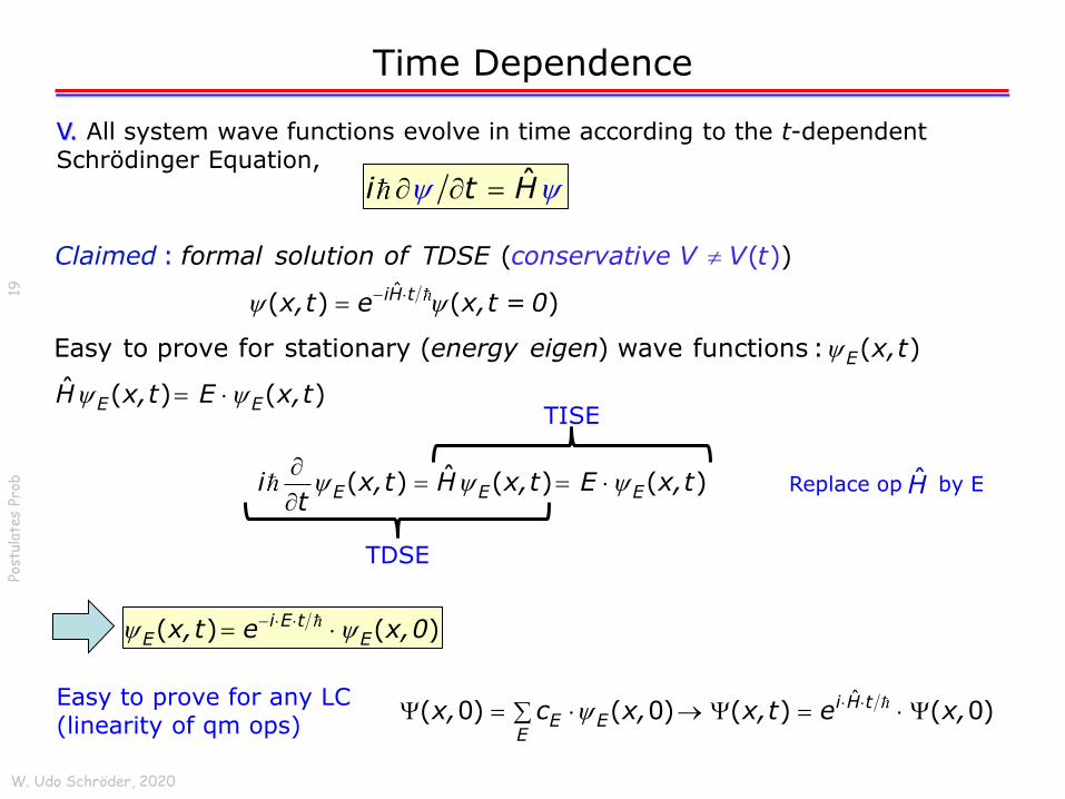
Time Dependence

V. All system wave functions evolve in time according to the t-dependent Schrödinger Equation,


Post

ulat

es

Prob

19

ˆi t H =

Easy to prove for stationary ( ) wave functions : ( )

ˆ ( ) ( )

E

E E

energy eigen x,t

H x,t E x,t

=

ˆ

( ( )

) ( )

: )

( iH t

conservative V V tC formal solution of TDSE

x,t e x, 0

la d

t =

ime

−

=

( ) ( )i E tE Ex,t e x,0 − =

ˆ( 0) ( 0) ( ) ( 0)i H t

E EE

x, c x, x,t e x, = → =

ˆ( ) ( ) ( )E E Ei x,t H x,t E x,tt

= =

TISE

TDSE

Replace op by EH

Easy to prove for any LC(linearity of qm ops)

Time Evolution of Particle Wave Packet


Post

ulat

es

Prob

20

( )2 2 2 2

2

:

ˆ0 : ( ) e

ˆ ( ) ( ) ( ) ( ) ( )2 2

ˆ( , ) ( , ) ( , ):

k

ki xk

k k k k

k k k k

Ensemble of particles with mass m

Plane waves at t x A are eigen functions of H

kH x V x x V x E x

m mx

f i x t H x t E x tThere ot

re

= =

− = + = + =

= =

( )

( ) ( )

0

1 42 2

2

0

( , 0) ,

1( ,0) ( )d ,

2

exp2 4

k

Free particle V const wave packet

central momentum k k

x f k x k

a aGaussian profile f k k k

+

−

=

=

=

= − −

( , ) ( , 0)

iE tk

k kx t e x t =

= =

Time Evolution of Particle Wave Packet


Post

ulat

es

Prob

21

( ) ( ) ( )

( )

0

1 42 2

2

0

( , 0) ,

1( ,0) ( )d , exp

2 42

1( ,0) ( ,0) d

2

k

k

Free particle V const wave packet central momentum k k

a ax f k x k Gaussian profile f k k k

i x f k i x kt t

+

−

+

−

= =

= = − −

= →

( )1 4 21

4

00 2 0

4 22 2

2 2 2

( )2 4( ) 1 exp

(2 )

ik

i k x tm kx t

x,t t ea m a a

m

te

i m

− −

−

= + − +

( )( )1 2: tan 2Phase factor ma t −=

( )

( )

1 42 2

22

ˆ

0

0

1( ) ( 0) exp

2 42

:

.

2

....

i H t

perfect square

a ax,t x, k k i k x dk

Evaluate integral by converting exponent to for q k k

i

ke i

Gaussian ntegra

tm

l

+

−

−

= = − − + −

=

−

→

( )

2

21

( , ) ( ,0)2

k

ki t

mx t f k e x

−

+

−

=

Linearity of operator

Spreading of Particle Wave Packet


Post

ulat

es

Prob

22

( ) ( )21 41 4 2

02 22 2 4 2

2 4( ) 1 exp

(2 )

i i k t gx phx

x,t t e ea m a a i m t

t

−

−

− = + − +

0 0

20

0 0

:

1

2

2

ph g

gk k

Traveling wave packet

Velocity of fundamental waves

Ephase velocity

k p

Velocity of superposition packet

kd d kgroup velocity

dk dk m m

=

= = =

= = =

Numerical solution

Summary: Measurement/Preparation (CI)


Post

ulat

es

Prob

23

Postulate: qm system can only be observed in an eigen-function (state) of the corresponding indication operator Â → Âa = a·a. Other states are not realizedOrthonormal “basis” sets {a} allow convenient expansions of wave functions.

QM makes no specific predictions for any single measurement of observable A, except: In any measurement, system will be found in one of the possible eigen states of Â with probability amplitude existing at time of measurement.

→Many independent measurements are distributed “statistically.”

BUT: Immediate repeat measurement of A on the same system give identical results, not a distribution!

→Wave function “collapses” (is suddenly reduced) to one component and frozen in that state.

→By measurement of A and selection of eigen value a (→state a), a system can be “prepared” in that state a. Repeat measurements yield same a.

Discontinuous change in t-dependent behavior of wf is not described by Schrödinger Equation.

Some (incompatible) observables cannot be measured simultaneously on systems, uncertainties of corresponding observables are (anti-)correlated.

Agenda: Quantum Mechanics Postulates & Consequences

Documents

Transcript of Agenda: Quantum Mechanics Postulates & Consequences