W&M ScholarWorks W&M ScholarWorks

Dissertations, Theses, and Masters Projects Theses, Dissertations, & Master Projects

2001

Age, Growth, and Mortality of Atlantic Croaker, Micropogonias Age, Growth, and Mortality of Atlantic Croaker, Micropogonias

undulatus, in the Chesapeake Bay Region undulatus, in the Chesapeake Bay Region

John R. Foster College of William and Mary - Virginia Institute of Marine Science

Follow this and additional works at: https://scholarworks.wm.edu/etd

Part of the Fresh Water Studies Commons, Oceanography Commons, and the Zoology Commons

Recommended Citation Recommended Citation Foster, John R., "Age, Growth, and Mortality of Atlantic Croaker, Micropogonias undulatus, in the Chesapeake Bay Region" (2001). Dissertations, Theses, and Masters Projects. Paper 1539617973. https://dx.doi.org/doi:10.25773/v5-s48f-je94

This Thesis is brought to you for free and open access by the Theses, Dissertations, & Master Projects at W&M ScholarWorks. It has been accepted for inclusion in Dissertations, Theses, and Masters Projects by an authorized administrator of W&M ScholarWorks. For more information, please contact scholarworks@wm.edu.

Age, Growth, and Mortality of Atlantic croaker, Micropogonias undulatus, in the

Chesapeake Bay region

A Thesis Presented to

The Faculty of the School of Marine Science The College of William and Mary

In Partial Fulfillment of the Requirements for the Degree of

Master of Science

By

John R. Foster

2001

This thesis is submitted in partial fulfillment of the requirements for the degree of

Master of Science

John R. Foster

Approved, June 2001

44-

Mark E. Chittenden, Jr., Ph.D.

Herbert M. Austin, Ph.D.

John A. Musick, Ph.D.

Peter A. van Veld, Ph.D.

TABLE OF CONTENTSPage

ACKNOWLEDGEMENTS.......................................................................................v

LIST OF TABLES.................................................... ' ..............................................vi

LIST OF FIGURES.................................................................................................viii

ABSTRACT............................................................................................................... x

GENERAL INTRODUCTION..................................................................................2

CHAPTER 1. Age Determination and Age Composition...................................8

INTRODUCTION.......................................................................................... 9

METHODS................................................ , .................................................11

RESULTS.................................................................................................... 16

DISCUSSION..............................................................................................36

CHAPTER 2. Size Composition and Growth................................................... 39

INTRODUCTION........................................................................................40

METHODS.................................................................................................. 42

RESULTS....................................................................................................45

DISCUSSION..............................................................................................61

CHAPTER 3. Mortality..........................................................................................64

INTRODUCTION........................................................................................65

METHODS.......................................................................... 67

RESULTS.................................................................................................... 71

DISCUSSION..............................................................................................77

LITERATURE CITED.............................................................................................79

VITA. 85

iv

ACKNOWLEDGEMENTS

I would like to thank my advisor, Mark E. Chittenden, Jr. for providing me with the opportunity and funding support to undertake this project and for his constructive review of this manuscript. I also thank the members of my committee: Herbert M. Austin, John A. Musick, and Peter A. van Veld, for their support and constructive review of this manuscript.

I thank James Owens, as well as the Anadromous Fishes workgroup and Juvenile Finfish Trawl Survey staff for their efforts in acquiring samples used in this study. I also thank Chris Bonzek, Claude Bain, the Virginia Marine Resources Commission, and the National Marine Fisheries Service for providing supplemental information on commercial catch and water quality data necessary to complete this project.

This study could not have been completed without the efforts of those brave souls who processed thousands upon thousands offish with me including Tom Ihde, Ann Sipe, Roy Pemberton, and especially, Beth Watkins. Thank you for your countless hours.

I am very thankful for additional field and laboratory experience afforded to me by the following persons: Herb Austin, Dee Seaver, David Hata, Deane Estes, Pat Geer, John Olney, Phil Saddler, Jim Goins, and Howard Kator. The knowledge, experience, and skills I have gained through work on your various projects are invaluable to me, and I thank you all.

To my friends at VIMS, thank you for friendship and support throughout my project. You know who you are, and I hope you know how much you mean to me.

Finally, to my parents, Bonnie and Ron, and family, thank you for your constant love and support. I would never have made it this far without you all. I would especially like to thank my great-grandfather, John R. Fuller, for taking the time to teach a little boy to fish. Thank you all.

v

TableLIST OF TABLES

Page

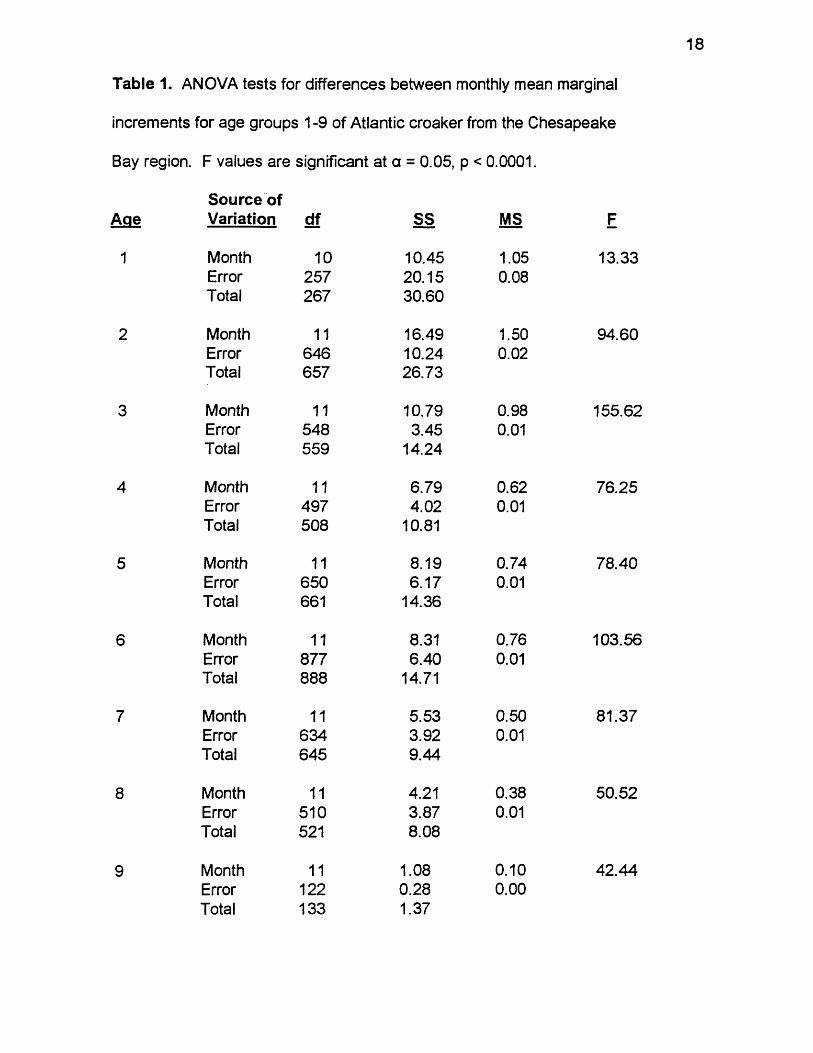
_ 1. ANOVA tests for differences between monthly mean marginalincrements for age groups 1-9 of Atlantic croaker from the Chesapeake Bay region. F values are significant at a = 0.05, p < 0.0001.................18

2. Observed minimum, maximum, Tg9, and mean ages of Atlantic croaker from the Chesapeake Bay region for each biological year and pooled over the entire sampling period, from March, 1998 - March, 2000. 20

3. Kolmogorov-Smirnov two-sample tests for differences between: 1)observed age compositions of Atlantic croaker from the Chesapeake Bay region in each biological year, and 2) each annual composition and the composition pooled over the entire sampling period, “ns" indicates non-significance at a = 0.05.................................................... 23

4. Kolmogorov-Smirnov two-sample tests for differences betweenobserved age compositions of Unusually Large Atlantic croaker from the Chesapeake Bay region collected in each biological year, March, 1988 - March, 2000. All results are significant at a = 0.05.................. 25

5. Observed and Adjusted Age compositions of Atlantic croaker fromSelected months during each biological year, March, 1998 - March, 2 0 0 0 ..............................................................................................................26

6 . Kolmogorov-Smirnov two-sample tests for differences betweenAdjusted Age compositions of Atlantic croaker from the Chesapeake Bay region from Selected months of each biological year of sampling. All results are significant at a = 0.05.......................................................29

7. Kolmogorov-Smirnov two-sample tests for differences betweenObserved and Adjusted age compositions from Selected months in each biological year, March, 1998 - March, 2000. "ns" indicates non­significance at a = 0.05............................................................................. 30

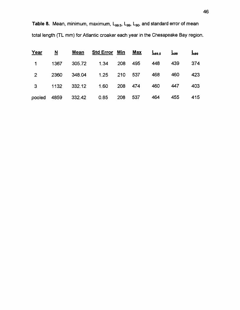
8 . Mean, minimum, maximum, L99.5, L99, L90, and standard error of meantotal length (TL mm) for Atlantic croaker each year in the ChesapeakeBay region................................................................................................... 46

9. Mean, minimum, maximum, and standard error of mean total length(TL mm) of female and male Atlantic croaker each year in the Chesapeake Bay region............................................................................47

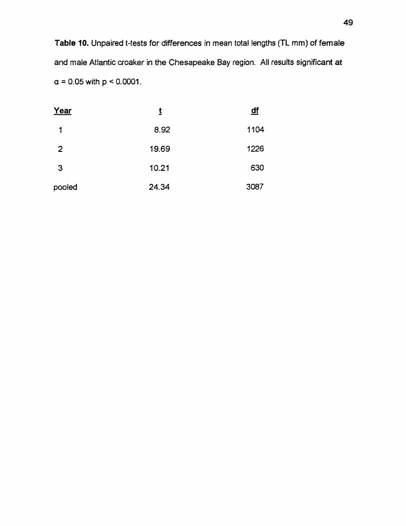
10. Unpaired t-tests for differences in mean total lengths (TL mm) offemale and male Atlantic croaker in the Chesapeake Bay region. All results are significant at a = 0.05 with p < 0.0001.................................49

11. Kolmogorov-Smirnov two-sample tests for differences between lengthfrequencies of Atlantic croaker from the Chesapeake Bay region each year, and between each year and all years pooled, "ns" indicates non-significance at a = 0.05.....................................................................51

12. Observed mean total length (TL mm), 95% confidence limits, standarderror, and sample size for age 1-10 Atlantic croaker collected in the Chesapeake Bay region............................................................................52

13. Minimum, maximum, and mean total length (TL mm), standard error, and sample size by sex for age groups 1-10 of Atlantic croaker in the Chesapeake Bay region with t-tests for between sex differences in mean size-at-age. "ns" indicates non-significance at a = 0.05. ...................................................................................................................... 53

14. von Bertalanffy growth parameter estimates with sample sizes, 95% confidence intervals (Cl) and coefficients of determination (r2) for each of three types of regression fitting. See text for explanation of fitting methods....................................................................................................... 55

15. Kimura (1980) likelihood ratio tests for between sex differences in estimates of von Bertalanffy growth parameters for Atlantic croaker in the Chesapeake Bay region by three different regression fits. See text for explanation of regression fits, "ns" indicates non-significance ata = 0.05....................................................................................................... 58

16. Kimura (1980) likelihood ratio tests for between sex differences in totallength-total weight relationship parameters. All differences were significant at a = 0.05, p < 000.1........................................................... 60

17. Estimates of total annual instantaneous mortality, Z, 1 - S, and S,based on maximum age methods for listed maximum ages................72

18. Catch-curve regression estimates of Z, 1 - S, and S, with coefficientsof determination (r2) and 95% confidence intervals (Cl), based on listed ages..............................................................................................................73

19. Estimates of instantaneous natural mortality rates, M, for Altantic croaker in the Chesapeake Bay region. See text for description of how parameters were estimated .............................................................76

vii

FigureLIST OF FIGURES

Page

1. Annual commercial landings and recreational citations for Atlantic croakerin Virginia, 1950 to 1998. Commercial landings data from National Marine Fisheries Service, Fisheries Statistics and Economics Division, Silver Spring, MD. Recreational citation data from Claude M. Bain, III, Virginia Saltwater Fishing Tournament, Virginia Beach, VA. The four numbers adjacent to arrows indicate sizes (lbs.) required for recreational citations; arrows point to the number of citations the first year that citation size was implemented. No citation was offered for Atlantic croaker from 1972 to 1976................................................................................................................ 5

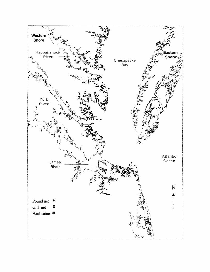
2. Locations of Atlantic croaker collections from pound-net, gill-net, and haul-seine fisheries in the Chesapeake Bay region....................................... 12

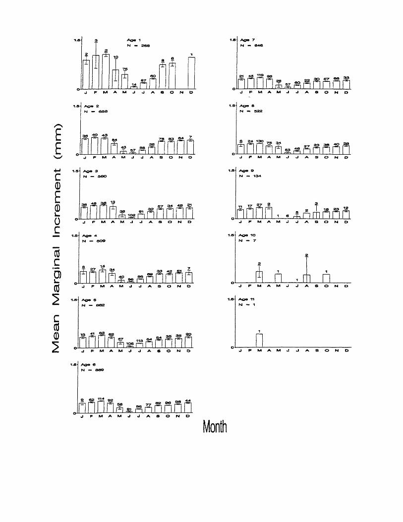
3. Mean marginal increments in Atlantic croaker by month for ages 1-11years. Error bars represent 95% confidence intervals about the mean. Numbers above bars represent monthly sample sizes......................... 17

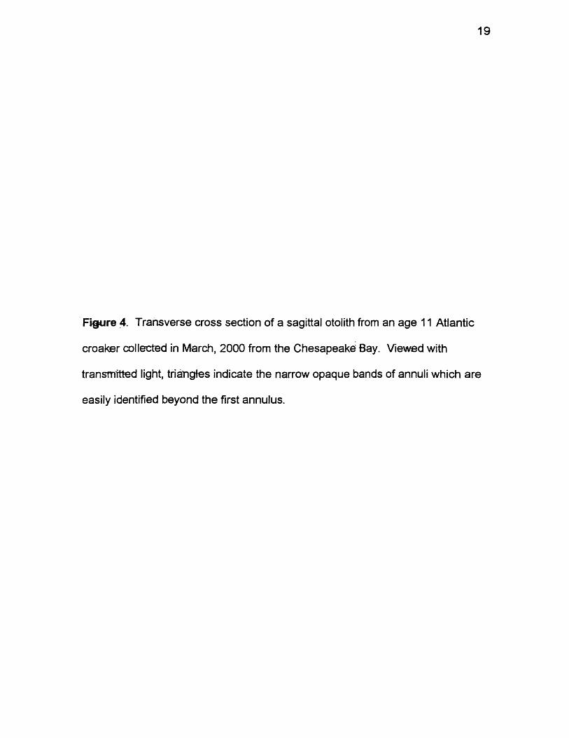
4. Transverse cross section of a sagittal otolith from an age 11 Atlanticcroaker collected in March, 2000 from the Chesapeake Bay. Viewed with transmitted light, triangles indicate the narrow opaque band of annuli which are easily identified beyond the first annulus...............................19

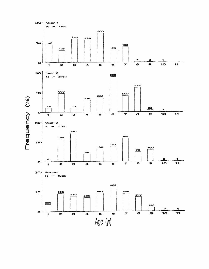
5. Observed age compositions in each biological year and pooled overall years, March, 1998 through March, 2000. Numbers above bars represent sample sizes................................ 2 2

6 . Observed age compositions in Unusually Large Atlantic croaker eachyear. Numbers above bars represent sample sizes.............................24

7. Adjusted and Observed Age compositions from Selected months ineach biological year of sampling............................................................. 27

8 . Observed and Adjusted catches based on Selected months, of Atlantic croaker in the Chesapeake Bay region by year-class, 1987 - 1998. ...................................................................................................................... 31

9. Observed age compositions in each biological year by Small (a), Medium (b), Large (c), Jumbo (d), Large and Jumbo (e), and ungraded (f) commercial grades. Numbers above bars represent sample sizes. ...................................................................................................................... 33

viii

10. Length (TL mm) frequency distributions of Atlantic croaker in the Chesapeake Bay region each year. Lengths are grouped by 25 mm size intervals. X-axis values are size interval midpoints, and numbers above bars correspond to sample sizes in each interval................................. 50

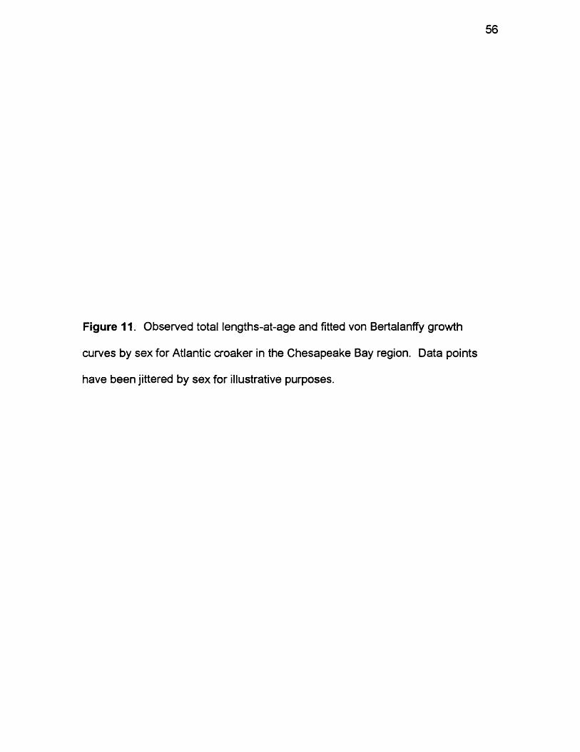
11. Observed total lengths-at-age and fitted von Bertalanffy growth curves by sex for Atlantic croaker in the Chesapeake Bay region. Data points have been jittered by sex for illustrative purposes..........................................56

12. Catch-curves, with regression estimates of Z, 1 - S, S, and r2 values, based on pooled Adjusted Age Composition over age ranges: A) 3-10, B) 3-9, C) 2-10, and D) 2-9. The indicates an influential observation. ...................................................................................................................... 75

ix

ABSTRACT

Sectioned otolith age determination methodology was validated by individual age groups using mean monthly marginal increment analysis incorporating one-way ANOVA significance testing. One annulus was formed each year for ages 1-9 with the narrow opaque band forming from April to June. Precision in age determination from sectioned otoliths was very high, 1 0 0 % within reader agreement and 97% between reader agreement.

Atlantic croaker were collected from commercial catches in the Chesapeake Bay region (N = 4862) from March, 1998 through March, 2000 to determine the impacts of relatively abundant unusually large fish on age, growth, and mortality information. Observed age compositions varied with biological year and by commercial grade. Ages 1-11 were recorded with ages 10 and 11 being rare.For unusually large fish (400+ mm TL), ages 4-11 were recorded, with ages 6-9 being abundant. Adjusted Age compositions varied with biological year but were similar to Observed Age compositions from Selected months in most years. Fluctuations occurred in year-class strength with year-classes prior to 1990 being much less important in Adjusted and Observed Age compositions from Selected months than the 1990 and subsequent year-classes.

There were differences in observed size compositions between sexes. While minimum sizes were similar, females were significantly larger on average than males, their pooled mean total lengths (TL) being 343 mm and 304 mm, respectively. Observed size-at-age varied by sex. Mean female size-at-age was significantly larger than males for ages 1-9. The von Bertalanffy growth model described growth of Atlantic croaker well though there were significant differences in growth between sexes. For females, Lx ranged from 399 mm to 535 mm, k ranged from 0.11 to 0.38, and t0 ranged from -4 .44 to -0 .95. For males, Lx ranged from 391 mm to 541 mm, k ranged from 0.08 to 0.18, and t0 ranged from -6 .7 to -4 .02. For sexes pooled, /.«, ranged from 403 mm to 541 mm, k ranged from 0.10 to 0.34, and t0 ranged from -5.01 to -1.19.

Estimates of total annual instantaneous rates, Z, based on maximum age methods ranged from 0.4 to 0.51, the lowest reported from the Chesapeake Bay region. Catch-curve regression estimates of Z ranged from 0.45 to 0.85, though estimates agreed well at 0.45 - 0.46 when an influential observation was deleted from calculations. Estimates of natural instantaneous mortality rates, M, varied by method ranging from 0.15 to 0.39,

x

Age, growth, and mortality

of Atlantic croaker, Micropogonias undulatus,

in the Chesapeake Bay region

GENERAL INTRODUCTION

Range

Atlantic croaker, Micropogonias undulatus, inhabit coastal waters in the

North Atlantic Ocean from the Bay of Campeche, Mexico to Cape Cod,

Massachusetts (Welsh and Breder, 1923; Chao, 1978). This demersal species is

highly abundant in coastal and estuarine waters over much of its range from

Middle Atlantic to Gulf of Mexico coasts (Joseph, 1972).

Life history

Atlantic croaker undertake seasonal migrations. In the Chesapeake Bay

region, they migrate into the Bay in the spring, from March to April, and leave in

the fall, from about September to November, to overwinter along the continental

shelf off the coasts of Virginia and North Carolina (Wallace, 1940; Haven, 1959).

Spawning begins as adults emigrate from the Chesapeake Bay and may

continue over a large area from waters near to and possibly including the mouth

of the Chesapeake Bay (Welsh and Breder, 1923) to shelf waters (Colton et al.,

1979; Morse, 1980; Norcross and Austin, 1988). Recent work also suggests that

some spawning may occur in the Bay itself (Barbieri et al., 1994b). Resulting

post larvae and small juveniles are transported into the Chesapeake Bay system

where they remain until migrating out of the Bay with the adults in the following

fall (Haven, 1957; Chao and Musick, 1977; Norcross, 1983).

Commercial fishery

While the Atlantic croaker is an important commercial resource in the

Chesapeake Bay region, annual landings have fluctuated greatly over the past

2

3

100 years (Joseph, 1972). Landings have ranged from a peak in 1945 of 26,000

metric tons to a low in 1968 of 2.8 mt (Rothschild et al., 1981; NMFS, personal

communication1). In Virginia, there have been three distinct periods of relatively

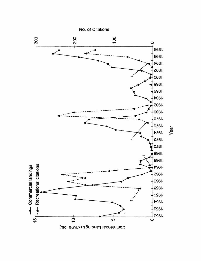
high landings separated by two periods of low landings, since 1950 (Figure 1).

The first period of relatively high landings occurred from 1954 to 1959 when

landings exceeded 2,000 metric tons annually with a peak of 6,440 occurring in

1957 (NMFS, personal communication1). Then from 1960 to 1974, landings fell

below 2,000 metric tons (NMFS, personal communication1). A second brief

episode of higher landings lasted from 1975 to 1978 with a peak of 3,901 metric

tons occurring in 1977 (NMFS, personal communication1). Then from 1979 to

1992, landings fell below 2,000 metric tons for the second time, and in 1982 only

54 metric tons were harvested (NMFS, personal communication1). The third

episode of increased landings began in 1993 and has continued through 1999

with an apparent peak in landings of 5,801 metric tons occurring in 1997 (NMFS,

personal communication1).

Occurrence of large Atlantic croaker

Associated with the three most recent periods of high commercial landings

in the Chesapeake Bay region has been the occurrence of unusually large

Atlantic croaker, fish more than 400mm in total length. The presence of these

large fish has been documented in previous reports (Hildebrand and Schroeder,

1928; Massmann and Pacheco, 1960; Ross, 1988; Barbieri, 1993), and in

recreational catch records from the Virginia Saltwater Fishing Tournament from

1 NMFS, OFFICE OF SCIENCE AND TECHNOLOGY, F/ST1, Room 12362, 1315 East-West Highway, Silver Spring, MD 20910

4

1958 to 1972 and 1976 to 1999 (Figure 1; Claude M. Bain, III, persona!

communication1). Massman and Pacheco (1960) collected Atlantic croaker from

the York River, Virginia in excess of 400 mm total length (TL) from 1950 to 1953

and from 1956 to 1958, and they collected fish greater than 500 mm TL in 1951,

1952, and 1958. Ross (1988) collected fish in North Carolina waters in excess of

400 mm TL and even 500 mm TL from 1979 to 1981. From 1958 to 1963, 931

citations for large Atlantic croaker, minimum weight of 0.91 Kg (2 lbs), were

awarded by the Virginia Saltwater Fishing Tournament; from 1977 to 1983, 548

citations for large fish, minimum weight of 1.82 KG (4 lbs), were awarded, and

from 1993 to 1998, 433 citations, minimum weight of 1.36 KG (3 lbs) were

awarded (Claude M. Bain, III, personal communication1). The year-classes that

produced these citation fish are not known, but they could reflect the episodic

occurrence of strong or dominant year-classes as suggested by Barbieri et al.

(1994a). Alternatively, Barbieri et al. (1994a) hypothesized that the proportional

increase and occurrence of these large fish resulted from good survivorship in

fish spawned early, July and August, coupled with lower survivorship in fish

spawned later, November and December, due to very low water temperatures in

nursery areas during the winter months (Massman and Pacheco, 1960; Joseph,

1972; Chao and Musick, 1977; Warlen and Burke, 1991). Early spawned fish

have been shown to have higher growth rates than fish spawned later in the year

(Warlen, 1982; Nixon and Jones, 1997) which could equate to very large adults.

1 Claude M. Bain, III, Virginia Saltwater Fishing Tournament, 986 South Oriole Drive, Suite 102, Virginia Beach, Virginia 23451

5

Figure 1. Annual commercial landings and recreational citations for Atlantic

croaker in Virginia, 1950 to 1998. Commercial landings data from National

Marine Fisheries Service, Fisheries Statistics and Economics Division, Silver

Spring, MD. Recreational citation data from Claude M. Bain, III, Virginia

Saltwater Fishing Tournament, Virginia Beach, VA. The four numbers adjacent

to arrows indicate sizes (lbs.) required for recreational citations. Arrows point to

the number of citations in the first year that citation size was implemented. No

citation was offered for Atlantic croaker from 1972 to 1976.

Com

mer

cial

lan

ding

sNo. of Citations

ooCO

ooC\J

oo

CO

8961*CO

oin in

( sq| 9vCHx) s6u!puen lepjaiuuioo

Yea

r

6

Status of age, growth, and mortality information

While there is much recent information on age and size compositions,

growth, and mortality of Atlantic croaker in the Chesapeake Bay and Middle

Atlantic regions, it is incomplete and possibly inaccurate as it does not include

exceptionally old, large fish. Barbieri et al. (1994a) described age, growth, and

mortality of Atlantic croaker in the Chesapeake Bay region. That report,

however, was based on a sample containing only one large fish, a fish just 400

mm TL. Presumably, large Atlantic croaker were rare in the Chesapeake Bay

region then. Without the ability to collect them, Barbieri et al. could not describe

the impact that the periodically occurring large fish might have on age, growth,

and mortality estimates. Ross (1988) reported on age, growth and mortality of

Atlantic croaker in North Carolina. His sample of 2,369 Atlantic croaker included

120 large fish with TL equal to or greater than 400 mm. Unfortunately, those 120

fish were aged using scales. Ross’ (1988) results may have contained

inaccuracies as problems with ageing Atlantic croaker based on scales have

been reported (Roithmayr, 1965; Joseph, 1972; Mericas, 1977; Barger and

Johnson, 1980; Barbieri, 1993; Barbieri et al., 1994a).

Description of thesis

There are three basic objectives to this study. The first is to determine the

age composition of unusually large Atlantic croaker, currently present in the

Chesapeake Bay region, using an accurate method for ageing based on

sectioned otoliths. As the presence of these large fish may significantly change

life history parameter estimates, the second objective is to revise information on

7

age, growth, and mortality of Atlantic croaker. The final objective then, is to

assess these changes through comparison with previous reports.

The thesis consists of three chapters. Topics related to age are covered

in the first chapter. Specifically, I validate the sectioned otolith ageing

method for ages 1-9 and provide information on the current age structure of

Atlantic croaker in the Chesapeake Bay region with a focus on the age structure

of unusually large fish. Based on the validated ageing method presented in

Chapter 1, growth is addressed in Chapter 2, and information on mortality is

provided in Chapter 3.

CHAPTER 1

Age Determination and Age Composition

8

INTRODUCTION

Studies on Atlantic croaker have used three main methods of age

determination. Early work reported ages from length frequency distributions

(Hildebrand and Cable, 1930; Gunter, 1945; Suttkus, 1955; Bearden, 1964;

Hansen, 1969; Christmas and Waller, 1973; Hoese, 1973; Gallaway and Strawn,

1974), and scale ageing (Welsh and Breder, 1923; Wallace, 1940; White and

Chittenden, 1977; Ross, 1988). Ageing Atlantic croaker with either of these two

methods is problematic, however. Difficulties with the length frequency method

arise from the protracted spawning period of Atlantic croaker (Morse, 1980;

Warlen, 1982; Barbieri et al., 1994b) and difficulty distinguishing modal groups at

older ages (White and Chittenden, 1977; Jearld 1983). Problems with scale-

based ageing include poorly defined marks (Barger and Johnson, 1980), irregular

frequency of marks (Haven, 1954), and difficulty in distinguishing marks

(Roithmayr, 1965; Joseph, 1972; Mericas, 1977). As neither the length

frequency nor scale method is wholly adequate (Barbieri et al., 1994a), sectioned

otolith ageing has often been used since 1980 (Warlen, 1982; Music and Pafford,

1984; Barger, 1985; Barbieri et al., 1994a). Sectioned otoliths have been found

superior to scales in definition and legibility of marks in two formal hard-part

comparisons, both of which concluded that sectioned otoliths were the best

structure for ageing Atlantic croaker (Barger and Johnson, 1980; Barbieri, 1993).

Validation of age determination methodology has been recommended for

each age group and population examined (Beamish and McFarlane, 1983).

9

10

Both scale and otolith ageing has been validated using marginal increment

analysis for Atlantic croaker populations in the South Atlantic and Middle Atlantic

Bights (Music and Pafford, 1984; Ross, 1988; Barbieri et al., 1994a). For

example, Ross (1988) reported validating scale-based ageing for ages 1 to 5,

and Barbieri et al. (1994a) validated otolith-based ageing for ages 1 to 7. Older

ages, however, have not been validated.

Many reports exist on Atlantic croaker age composition. While differing in

geographic region, sampling regime, and age determination methodology, they

often are similar in that they consist of predominantly young fish. For example,

the maximum ages reported by Music and Pafford (1984) in Georgia waters was

5 years, but less than 1 % of the fish were over age 2. Barger (1985) reported a

maximum of age 8 in the Northern Gulf of Mexico with about 7% over age 3.

Ross (1998) reported age 7 as the maximum, but only 9% were over age 3. Only

Barbieri et al. (1994a) collected a relatively large number of older fish. The

maximum age in that study was 8 with 35% of the fish over age 3 and 13% over

age 5.

Given the occurrence of unusually large, potentially older, Atlantic croaker

in the Chesapeake Bay region in recent years (see General Introduction),

validating ageing techniques for older age groups and obtaining an age structure

for a population with many older individuals may be possible. In this section, I

validate an otolith-based ageing method and present age composition data with a

focus on older individuals.

METHODS

Collection of Fish

Atlantic croaker were collected twice monthly from 1998 to 2000 from

catches of commercial pound-net, haul-seine, gill-net, and trawl-net fisheries

along the Western Shore and Eastern Shore of the Chesapeake Bay region

(Figure 2). Collections consisted of one 22.7 kg (50lb) box offish from each

available commercial grade: Small, Medium, Large, and Jumbo. While boxes

were not selected randomly, most of the variation in length compositions has

been shown to be captured by within-box variation for pound-net and haul-seine

catches of Atlantic croaker (Chittenden, 1989).

Age Determination, Validation, and Precision

Ages were determined from transverse cross sections of saggital otoliths.

For every fish, both saggital otoliths were removed and stored dry. The right or

left otolith were randomly selected and a transverse cross section was cut

through the core with a pair of diamond blades using a Buehler low-speed Isomet

saw. Resulting sections, about 0.75 mm thick, were mounted on glass slides

with Crystalbond™ 509 (polyethylene phthalate) and read under a dissecting

scope with transmitted light.

Ages were based on counts of annuli. The annulus in Atlantic croaker is a

bipartite mark consisting of a narrow opaque band and a broad translucent band

when viewed under transmitted light (Barbieri et al., 1994a). The edge of the

annular mark is considered to be the proximal edge of the distinct narrow opaque

band, except for the first annulus which is a less distinct opaque band that may

11

12

Figure 2. Locations of Atlantic croaker collections from pound-net, gill-net, and

haul-seine fisheries in the Chesapeake Bay region.

Western * ̂ ^Shore \ *♦

' 'i' x V

Rappahanock > * "River

^ } > /« . >" \g \x£r'5 k •

\ Vv

r .^, i y■k w ^ ;; j}

YorkRiver

J }>“ H k / H ? r 3 »

JamesRiver

ChesapeakeSay

Eastern -vj Shore*^i

>*%■

y*

^ i- / r jX V v

. V

W 'V / ,

AtlanticOcean

13

not be completely separate from the otolith core region (Barbieri et al.t 1994a).

As the average biological birthdate for Atlantic croaker in the Chesapeake Bay

region occurs in September, following Barbieri et al., 1994a), I used September 1

was used as an arbitrary birthdate for promoting fish from one age-group to the

next. All sectioned otoliths were read twice by two readers.

Presumptive annual marks were validated by age group using the

marginal increment method (Bagenal and Tesch, 1978), where the marginal

increment is the distance from the proximal edge of the last annulus (defined

above) to the outer edge of the section along the ventral side of the sulcal

groove. Marginal increments were measured using a calibrated digital imaging

system and SPOT RT software version 3.0 (Diagnostic Instruments, Inc., 1997).

Differences between monthly mean marginal increments were evaluated by one

way ANOVA (Zar, 1984) for each individual age group.

Ageing precision was evaluated by percent agreement. Otolith sections

from one hundred fish, ranging in size and age from 225-480mm TL and 1-9

years, were randomly selected from the total sample and read twice by two

readers. Percent agreement was then calculated for both within reader and

between reader agreement.

Age Composition

To describe age composition, the range of ages, mean age, age

frequency distribution, and T99, the 99th percentile of that distribution, were given

for each biological year and for all fish pooled over all years. Biological years

started on September 1 and ended on August 31. Collections were made during

14

three biological years: Year 1 (03/98-08/98), Year 2 (09/98-08/99), and Year 3

(09/99-03/00). Observed age compositions were also reported for each

commercial grade by biological year. As the Virginia Marine Resources

Commission only reports commercial catches for Small, Medium, and Large

grades, a frequency distribution was also constructed by pooling Large and

Jumbo grades. An additional age frequency distribution was given for each

biological year for Unusually Large fish, fish 400mm TL or greater. Differences in

mean age among years were evaluated by one way ANOVA and Kolmogorov-

Smirnoff two sample tests (Zar, 1984) were used to evaluate inter-annual

differences between observed age compositions, observed age compositions by

commercial grade, and observed age compositions of Unusually Large fish.

Ratio estimates (Cochran, 1977) were used to construct Adjusted Age

Compositions to better reflect the actual composition of the commercial catch in

Virginia. Estimates were based on Virginia Marine Resources Commission

(VMRC) reports on total landings of each commercial grade each month. To

construct an Adjusted Age Composition, for each year the number of fish in each

age group was estimated for each market grade for each month and then

summed across months and grades as:

Ni= I(sum for jk) Nijk = ( nijk/ wjk) * Wjk,

where

Nj is the adjusted number offish age / in Virginia’s total annual commercial catch,

Njjk is the adjusted number of fish age / in commercial grade j caught in month k,

n,jk is the number of fish age / in the sample collected from grade j in month k,

15

Wjk is the total weight of the sample collected from grade j in month k, and

Wjk is the weight of the total commercial catch for grade j in month k.

Only observed ages and weights from Selected months in which Small, Medium,

and Large grades were available were used to construct the Adjusted Age

Compositions. Selected months were May - July, and September - November in

1998, April - June, October, and November in 1999, and January - March in

2000. Kolmogorov-Smirnoff (KS) two-sample tests (Zar, 1984) were used to

evaluate differences between Observed and Adjusted Age compositions within

and between years. Only Observed Age frequencies from Selected months were

used in these comparisons.

To evaluate year-class strengths, individual age groups were

converted to year-classes in each biological year. Observed and Adjusted Age

Compositions were qualitatively evaluated for patterns in relative abundance of

year-classes.

RESULTS

Age Validation and Precision

Atlantic croaker form one annulus a year, from April through June in the

Chesapeake Bay region. Only one trough in monthly mean marginal increment

values was present for ages 1-9 (Figure 3), indicating that only one annulus is

formed each year. Mean values generally declined beginning in April signaling

the onset of mark formation at each age. Mean values continued to decline

through May to a minimum in June, indicating peak annulus formation in June.

Mean values increased through July and August to a relatively stable plateau that

lasted from September to March, indicating little or no otolith growth from

September through March. ANOVA found significant differences between

monthly means at each age (Table 1). Too few fish were collected to validate

age beyond age 9.

Sectioned otolith age determination was very precise. Within reader

agreement was 100% for reader 1 and for reader 2. Between reader agreement

was 97% for both the first and second readings. The few disagreements reflect

difficulties interpreting the otolith edge and were never greater than one year.

Annuli were generally easily recognized even at the oldest ages (Figure 4).

Age Composition

Observed age compositions were generally similar overall, though they

varied a bit by biological year. Ages ranged from 1 to 10 years in the first two

years, from 1 to 11 in the third year (Table 2). Age 11 was the oldest observed

age recorded. Second highest ages were 9 years in the first two years and 10 in

16

17

Figure 3. Mean marginal increments in Atlantic croaker by month for ages 1-11

years. Error bars represent 95% confidence intervals about the mean.

Numbers above bars represent monthly sample sizes.

Mean

Ma

rgin

al

Incre

me

nt

(mm

)*

Age 1 M — 268

*

1*X̂ Lao

anj f m a m j j a s o n d

Age 2

N — 668

3<3 ^ 384ifl 78 83 84on

J f m a m j j a s o n d

Afle 3

IM — 660

J F M A M J J A S O N D

A g e 4 N — 609

Q40 86 r“ *i

r£i.g> n i l nnftftJ J A S O N D

N — 662

A g e 7 IM — 846

21 4 6 2 2 9 6 3 0 6 7 6 8 M

0 1 I I I I I I 1 l - M r * i 1 1 I I I I I 1] I I 1 J F M A M J J A 8 0 N D

8- A O® 8N — S2 2

. ft ff Ha ft* * a a a a nJ F

6- A o ® 9 N — 1 3

11 1? j0nnr

1 4 A M J J A S O N D

4

1ft,.J F

5 A O® l O N — 7

F

4 A M J J A S O N D

2

i

] n < n nJ F »

5- A g a 11 N — 1

4 A M J J A 8 O N D

t

J f m a m j j S O N D J F M A M J J A S O N D

AO® 6n — a

m f l H ^ n n n n nM J J A O N D

Month

18

Table 1. ANOVA tests for differences between monthly mean marginal

increments for age groups 1-9 of Atlantic croaker from the Chesapeake

Bay region. F values are significant at a = 0.05, p < 0.0001.

Source ofAge Variation df s s MS

1 Month 1 0 10.45 1.05Error 257 20.15 0.08Total 267 30.60

2 Month 11 16.49 1.50Error 646 10.24 0 .0 2Total 657 26.73

3 Month 11 10.79 0.98Error 548 3.45 0 .01Total 559 14.24

4 Month 11 6.79 0.62Error 497 4.02 0 .01Total 508 10.81

5 Month 11 8.19 0.74Error 650 6.17 0 .01

Total 661 14.36

6 Month 11 8.31 0.76Error 877 6.40 0 .01

Total 8 8 8 14.71

7 Month 11 5.53 0.50Error 634 3.92 0 .01

Total 645 9.44

8 Month 11 4.21 0.38Error 510 3.87 0 .01

Total 521 8.08

9 Month 11 1.08 0 .1 0

Error 1 2 2 0.28 0 .0 0

Total 133 1.37

F

13.33

94.60

155.62

76.25

78.40

103.56

81.37

50.52

42.44

19

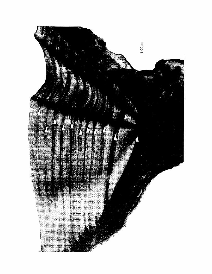
Figure 4. Transverse cross section of a sagittal otolith from an age 11 Atlantic

croaker collected in March, 2000 from the Chesapeake Bay. Viewed with

transmitted light, triangles indicate the narrow opaque bands of annuli which are

easily identified beyond the first annulus.

20

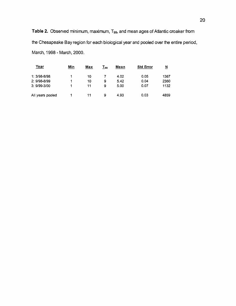
Table 2. Observed minimum, maximum, T99, and mean ages of Atlantic croaker from

the Chesapeake Bay region for each biological year and pooled over the entire period,

March, 1998 - March, 2000.

Year Min Max I 99 Mean Std Error N

1: 3/98-8/98 1 10 7 4.02 0.05 13672: 9/98-8/99 1 10 9 5.42 0.04 23603: 9/99-3/00 1 11 9 5.00 0.07 1132

All years pooled 1 11 9 4.93 0.03 4859

21

the third year. T99 was 7 years in year 1 and 9 in years 2, 3, and for all years

pooled. Mean age was 4.02 in year 1, 5.42 in year 2, 5.0 in year 3, and 4.93 for

all years pooled. Differences in mean ages between years were significant

(ANOVA, F = 191.22, df = 4858, p < 0.0001).

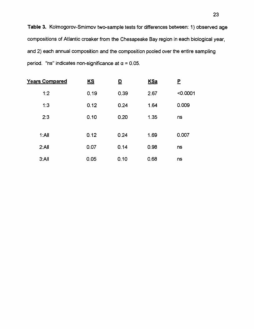
Observed Age frequency distributions differed from year to year. Age 5

was most common in year 1, making up 22% of that distribution (Figure 5), but

ages 1, 3 and 4 each made up 15 - 21 %. Age 6 was most abundant in year 2,

accounting for 27% of that frequency distribution. Age 3 was the most common

in year 3, making up 22% of that distribution. Observed Age frequency

distributions were significantly different between years 1 and 2, 1 and 3, and 1

and the pooled distribution (Table 3). Differences were not significant between

years 2 and 3 nor between 2 or 3 and the pooled distribution.

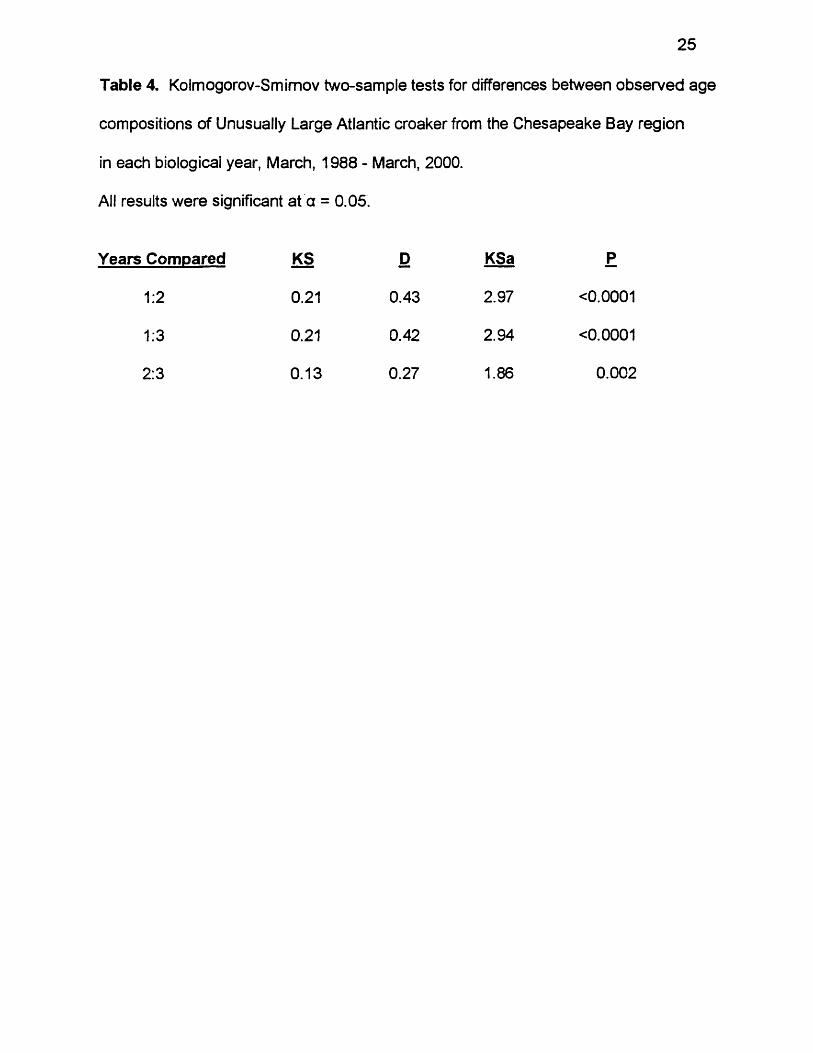
Age composition of the Unusually Large fish varied by year. Ages ranged

from 4 to 9 in year 1, though most fish were ages 5 - 7 (Figure 6 ). Age 7 alone

made up almost 65% of the Unusually Large then. Ages ranged from 4 to 10 in

year 2, though most fish were ages 6 - 8 . Ages 8 and 6 were the most frequent

ages, making up 42% and 27%, respectively. Ages ranged from 4 to 11 in year

3, with no fish being age 10. Most fish were ages 6 - 9 . Ages 7 and 9 were the

most frequent making up 28 - 32%. KS tests found significant differences in age

frequencies between the three years (Table 4).

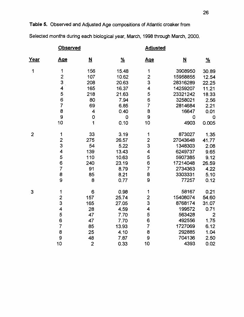
Adjusted Age Compositions varied greatly between biological years. Ages

1, 3, and 5 were most abundant in year 1, making up 31%, 22%, and 18%,

respectively (Table 5, Figure 7). Ages 2 and 4 each made up 11 - 13%. Ages 2

22

Figure 5. Observed age compositions in each biological year and pooled over

all years, March, 1998 - March, 2000. Numbers above bars represent sample

sizes.

Fre

qu

en

cy

(%)

301 3 6 7

300

166

o 10 113

30

IS

Y e a r 2

rsj *• 2360

333

633

7 0

o

216

2 0 2

33I 12 3 4 5 6 7 8 9 1 0 11

30

16

Year 3

M — 1 1 3 2

108 lOO70

2 3 5 6 7 8 9 lO 11

30

1 5

Pooled

N — 4869

8 8 S

658 663560 600

268

623

136

1 1 7 1

8 & io 11

Age(yr)

23

Table 3. Kolmogorov-Smimov two-sample tests for differences between: 1) observed age

compositions of Atlantic croaker from the Chesapeake Bay region in each biological year,

and 2 ) each annual composition and the composition pooled over the entire sampling

period, "ns" indicates non-significance at a = 0.05.

Years Compared KS D KSa P

1 :2 0.19 0.39 2.67 <0 .0 0 0 1

1:3 0 .1 2 0.24 1.64 0.009

2:3 0 .1 0 0 .2 0 1.35 ns

1: All 0 .1 2 0.24 1.69 0.007

2:AII 0.07 0.14 0.98 ns

3:AII 0.05 0 .1 0 0 .6 8 ns

24

Figure 6 . Observed age compositions in Unusually Large Atlantic croaker each

year. Numbers above bars represent sample sizes.

Fre

qu

en

cy

(%)

3 0

1 s

51Year 1

N — 79

13

11

3 0

1 5

8

255Year 2

N = 607 162

54

112

16

10 11

lO 11

393 0 Year 3

137

2221

1110

Age (yr)

25

Table 4. Kolmogorov-Smimov two-sample tests for differences between observed age

compositions of Unusually Large Atlantic croaker from the Chesapeake Bay region

in each biological year, March, 1988 - March, 2000.

All results were significant at a = 0.05.

Years Compared KS D KSa P

1 :2 0 .2 1 0.43 2.97 <0 .0 0 0 1

1:3 0 .2 1 0.42 2.94 <0 .0 0 0 1

2:3 0.13 0.27 1 .8 6 0 .0 0 2

26

Table 5. Observed and Adjusted Age compositions of Atlantic croaker from

Selected months during each biological year, March, 1998 through March, 2000.

Observed Adjusted

Age N % Age N %

1 156 15.48 1 3908950 30.892 107 10.62 2 15958855 12.543 208 20.63 3 28316289 22.254 165 16.37 4 14259207 1 1 .2 15 218 21.63 5 23321242 18.336 80 7.94 6 3258021 2.567 69 6.85 7 2814684 2 .2 18 4 0.40 8 16647 0 .0 19 0 0 9 0 0

1 0 1 0 .1 0 1 0 4903 0.005

1 33 3.19 1 873027 1.352 275 26.57 2 27043648 41.773 54 5.22 3 1348303 2.084 139 13.43 4 6249737 9.655 1 1 0 10.63 5 5907385 9.126 240 23.19 6 17214048 26.597 91 8.79 7 2734363 4.228 85 8 .21 8 3303331 5.109 8 0.77 9 77257 0 .1 2

1 6 0.98 1 58167 0 .2 1

2 157 25.74 2 15408074 54.603 165 27.05 3 8768174 31.074 28 4.59 4 199572 0.715 47 7.70 5 563428 2

6 47 7.70 6 492556 1.757 85 13.93 7 1727069 6 .1 2

8 25 4.10 8 292885 1.049 48 7.87 9 704136 2.50

1 0 2 0.33 1 0 4393 0 .0 2

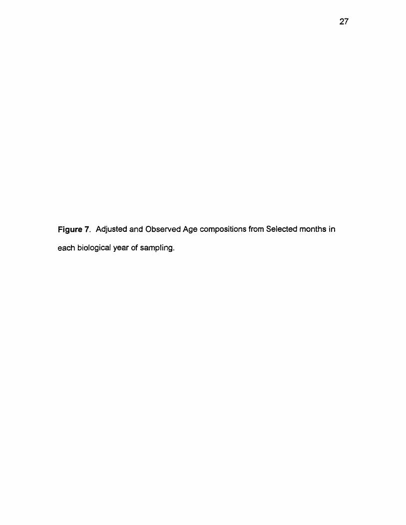
Figure 7. Adjusted and Observed Age compositions from Selected months

each biological year of sampling.

dr - .

c o

U3

CO

CM

s SB SB

CO

in

CO

CM

CO

CM

CO

CM

cc

r^-

CO

mCO

m

t 3?

CO

CM

CO

CM

*3(%) Aouenbajj

Age

(yr)

28

and 6 were the most abundant by far in year 2, making up 42% and 27%,

respectively. No other age made up more than 10%. Ages 2 and 3 made up

most of the distribution in year 2, at 55% and 31%, respectively. KS tests found

significant differences between years in the Adjusted Age frequencies (Table 6 ).

Observed Age compositions based on Selected months and Adjusted Age

compositions were generally similar within years. Although Observed Age and

Adjusted Age specific frequencies sometimes differed (Table 5) by as much as

15.4% in year 1 (for age 1), 28.84% in year 2 (for age 1), and 28.86% in year 3

(for age 2), the general age frequency patterns did appear similar (Figure 7). KS

tests found significant differences between Observed Age and Adjusted Age

compositions based on Selected months in year 3 but not in years 1 or 2 (Table

7). Despite the significant difference in year 3, both Observed Age and Adjusted

Age frequencies based on Selected months do show the same basic pattern in

that year. Ages 2 and 3 were much more important than the other older ages,

and both Observed Age and Adjusted Age showed similar patterns in those other

older ages. The detected significance may, therefore, not have strong biological

implications; rather it may reflect large sample sizes.

Atlantic croaker year-class strength seemed to vary greatly over the period

1987 - 1998. The 1987, 1988, and 1989 year-classes each made up only a small

part of either the Observed Age or Adjusted Age based on Selected months, in

any of the three years (Figure 8 ). These year-classes were about 8 - 1 1 years of

age during the study period, so that either these year-classes were always weak,

or they passed out of the fishery by age 8 . The 1992 year-class

29

Table 6 . Kolmogorov-Smimov two-sample tests for differences between Adjusted Age

compositions of Atlantic croaker from the Chesapeake Bay region from Selected months

of each biological year of sampling. All results were significant at a = 0.05.

Years Compared KS D KSa P

1 :2 0.16 0.32 2.23 <0 .0 0 0 1

1:3 0.16 0.31 2.15 0 .0 0 0 2

2:3 0 .2 2 0.43 3.00 <0 .0 0 0 1

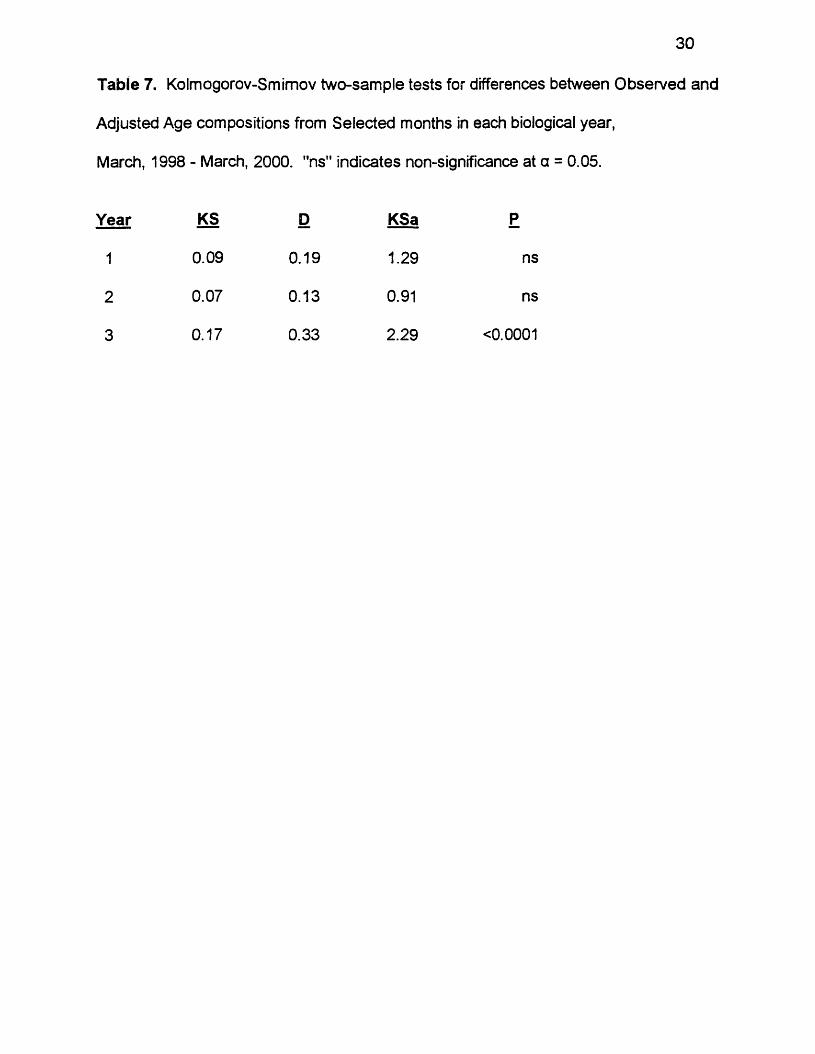
Table 7. Kolmogorov-Smimov two-sample tests for differences between Observed and

Adjusted Age compositions from Selected months in each biological year,

March, 1998 - March, 2000. "ns" indicates non-significance at a = 0.05.

Year KS D KSa P

1 0.09 0.19 1.29 ns

2 0.07 0.13 0.91 ns

3 0.17 0.33 2.29 <0 .0 0 0 1

31

Figure 8 . Observed and Adjusted catches based on Selected months, of Atlantic

croaker in the Chesapeake Bay region by year-class, 1987 - 1998.

Freq

uenc

y (%

)

Observed catches, Year 1 Adjusted catches, Year 1

□ a1987 1988 1989 1990 1991 199E 1993 1994 1995 1996 1997 1998 1967 1988 1989 1990 1991 1992 1993 1994 1995 1996 1997 1998

Observed catches, Year 2 ® i Adjusted catches, Year 2

JZL n i i jm r~i1987 1988 1989 1990 1991 1992 1993 1994 1995 1996 1997 1998 1987 1988 1989 1990 1991 1992 1993 1994 1995 1996 1997 1998

Observed catches, Year 3

30-

Adjusted catches, Year 3

n1987 1988 1989 1990 1991 1992 1993 1994 1995 1996 1997 1998 1987 1988 1989 1990 1991 1992 1993 1994 1995 1996 1997 1998

Year-class

32

was apparently a very strong year-class. It made up roughly 18 - 28% of the

Observed catch during the study period, and 18 - 25% of the Adjusted catch in

years 1 and 2, though this year-class was 5 - 7 years old then. Except for the

Adjusted catch in year 3, the 1992 year-class was generally at least as strong as,

generally much stronger than, any of the year-classes following it from 1993 -

1996. The 1990 and 1991 year-classes were apparently also strong year-classes.

They made up 8 - 20% of the Observed catch in the study period, a percentage

that was generally about as large, or larger than, most of the year-classes

following them from 1993 - 1996, this despite the age, 6 - 9 years, of the 1990

and 1991 year-classes in the period 1998-2000. The 1990 and 1991 year-classes

were similarly strong in the Adjusted catch in years 2 and 3, though not in year 1.

It was the 1990 and 1991 year-classes that produced most of the Atlantic croaker

I collected at ages 7 - 9 .

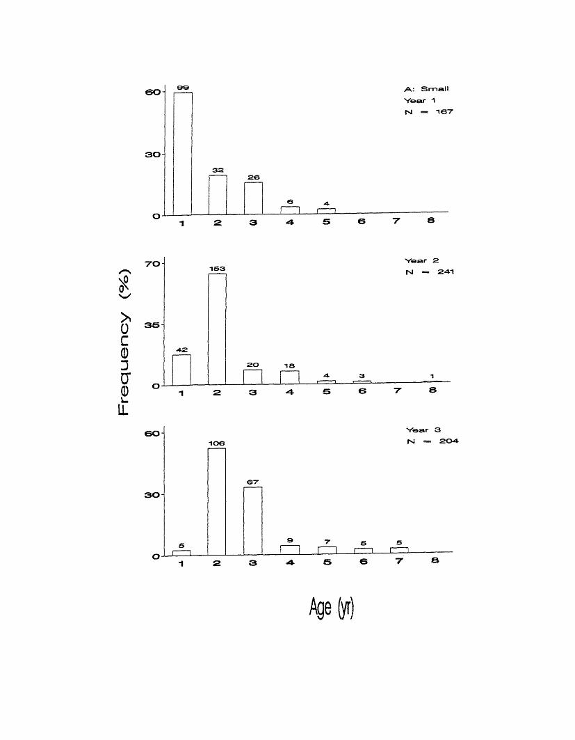
Age Composition by Commercial Grades

Atlantic croaker showed considerable inter-annual variation in age

compositions within commercial grades. In Small grade fish, ages ranged from 1

to 5 in year one, with age 1 comprising almost 60% of the distribution (Figure 9a).

Ages ranged from 1 to 6 in year 2, with age 2 comprising over 63% of that

distribution. Ages ranged from 1 to 7 in year 3, with ages 2 and 3 making up

52% and 33% of that distribution respectively.

For Medium grade fish, ages ranged from 1 to 7 in year 1, with a single

age 10 fish (Figure 9b). Most of that distribution was made up of ages 1 to 5 with

age 3 being most common at 28%. Ages ranged from 1 to 9 in year 2, though

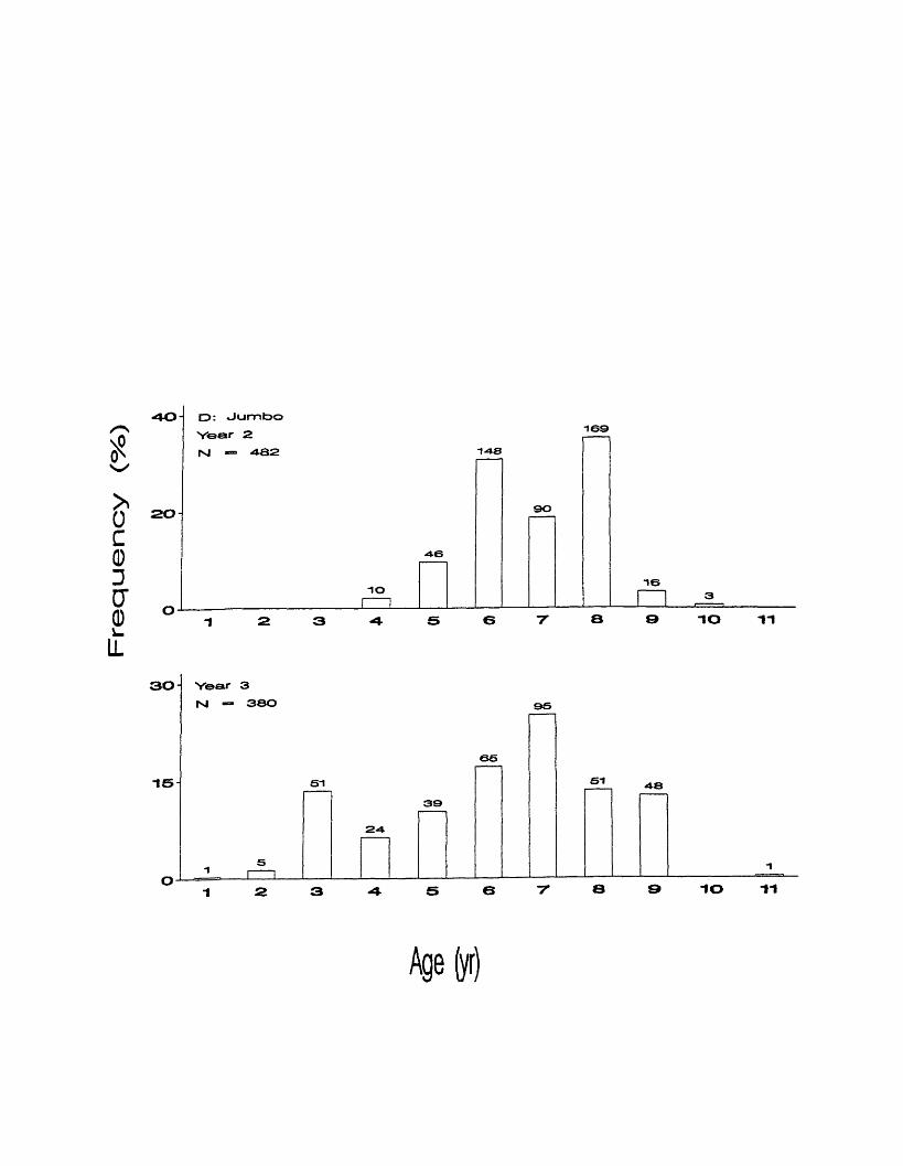
Figure 9. Observed age compositions in each biological year by Small (a),

Medium (b), Large (c), Jumbo (d), Large and Jumbo (e), and ungraded (f)

commercial grades. Numbers above bars represent sample sizes.

Fre

quency

(%)

A: Small

Year 1 INI = 167

60

30

32

70

35

~I63

-4-2

Year 2 INI — 2 - 4 1

20 ia

60106

67

30-

Age(yi)

Fre

quency

(%)

30 1 0 5B: Medium

Vear 1

rsi = 376

7062

66

15- 5 2

-IS

I !6 9 lO

40 98 Year 2

N — 260

2 0 4 64-a

1© 10

11 11

o no

02 Vear 3

fs| — 240

66

2 0

2 5

12 1 31 7

-to

Agefyr)

Fre

quency

(%)

30

-is-

o

40*

2 0

O

30

15'

C: Large

Veeir 1 j s j — 8 1 - 4 .

2 - 4 0

1571 - 4 6

109 110

21 23

2 3 -4- 5 6 7 8 Q 10

Year 2

N •“ 868 2 9 1

1 1 3 120 1 1 5 123

66

28

2 3

io

5 6 7 8 9 IO

V e e r 3

N «=• 291 7 7

- 4 5 4-437

33

23

1-4 1 6

1 2 3 4 5 6 7 8 9 IO

Age(yi)

Fre

quency

(%)

D: Jumbo

Year 2

rsl — 482

9 0SO-

16io

“IO -»1

3 0 Year 3

M — 380 95

6 6

-is si SI 4 - 8

39

24

s 6 7 8 9 10 11

Age(yr)

Fre

quency

(%)

301 EE: Large and Jumbo

Year 1 rsi =» eiA

240

1 5 7146

15 1 0 9 110

21 2 3

IO 11

40 Yaar 2fsj — 1350

4 3 9

2 01 6 6

1 2 3

662 8

2 9 2

2 0 6

2 6

HZH ±5 6 7 8 9 IO 11

30 Year 3

Nl — 671 172

IIO

15 88 9 2

7 2 7 4

4 0

1 92 1

9 IO 11

Age(yr)

Fre

quency

(%)

50 F: Ungraded

Year 1

N - 10

IO

30 Year 2

rsl — 5091 - 4 3

66

292 3 2 1

61 1

1 2 3 4

139

7 6

5I 1

30

IO

Age(yr)

34

ages 2, 4, and 6 were most common comprising 38%, 18%, and 18.5%. Ages

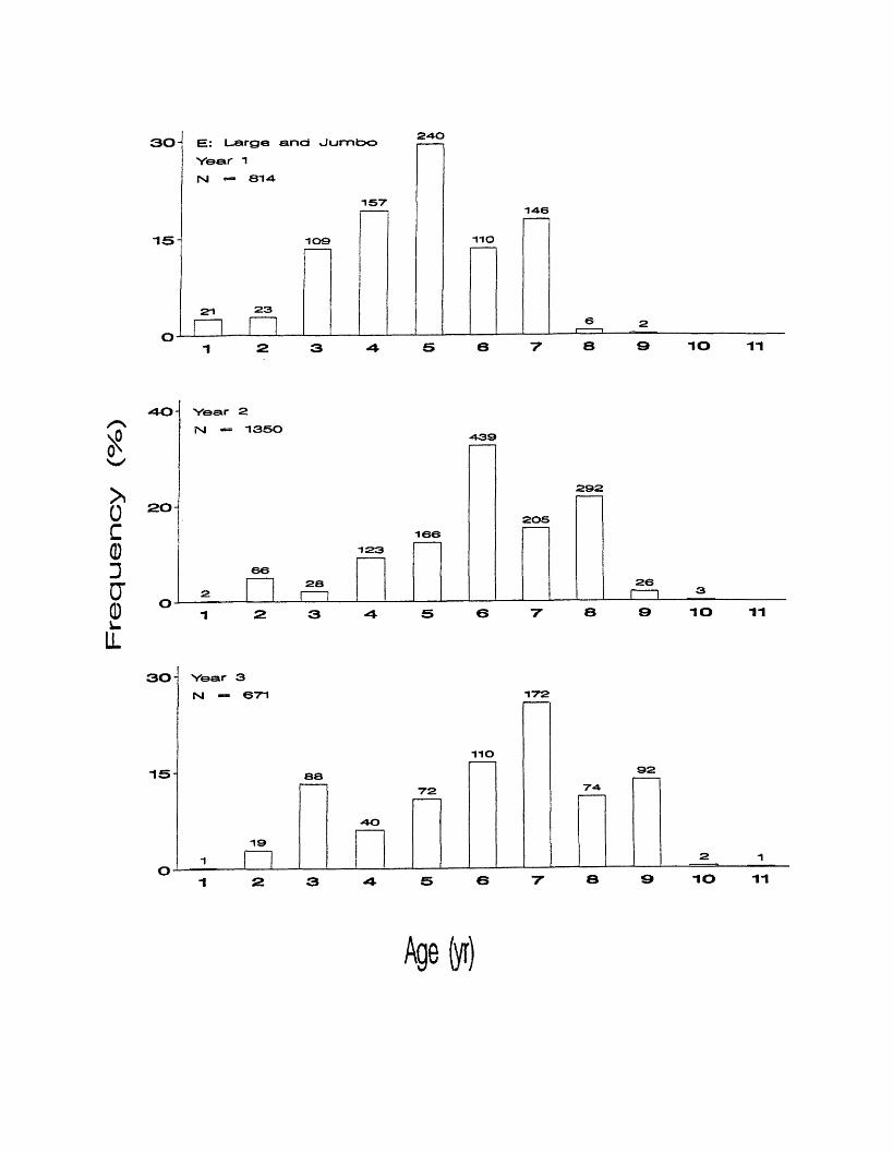
ranged from 1 to 9 in year 3, though ages 2 and 3 made up most of the

distribution, 28% and 38%, respectively.

In Large grade fish, ages ranged from 1 to 9 in year one (Figure 9c). Age

5 was most abundant making up 29% of that distribution, although ages 3, 4, 6,

and 7 were also common. Ages ranged from 1 to 9 in year 2, with age 6 fish

making up 34% of the distribution. Ages 4, 5, 7, and 8 were also common. Ages

ranged from 2 to 10 in year 3. Age 7 was most common accounting for 26%.

Ages 3, 5, 6, and 9 were also abundant although each made up less than 15%.

Jumbo grade fish were not collected in the first year. Ages ranged from 4

to 10 in year 2, with ages 6 and 8 making up 31% and 35%, respectively (Figure

9d). Ages ranged from 1 to 11 in year 3, with age 10 being absent. Age 7 was

most abundant, making up 25%. Ages 3, 6, 8, and 9 were also common making

up 13 -17% each.

The pooled Large and Jumbo grades age composition was identical to the

Large grade in the first year, as jumbo fish were not collected that year (Figure

9e). Ages ranged from 1 to 10 in year 2, with ages 6 and 8 making up 33% and

22%, respectively. Ages 5 and 7 were also common making up 12% and 15%.

Ages ranged from 1 to 11 in year 3. Age 7 was most common making up 26%.

Ages 3, 5, 6, 8, and 9 were also abundant accounting for 10 -16% each.

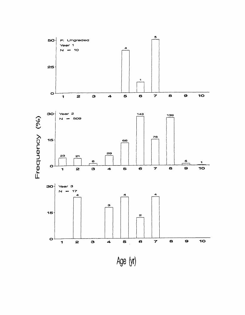
In ungraded fish, ages ranged from 5 to 7 in year one (Figure 9f). Ages 5 and 7

were most abundant making up 40% and 50%, respectively. Ages ranged from 1

to 10 in the second year, with ages 6 and 8 making up over half the distribution at

35

28% and 27%, respectively. Age 2 and ages 4 - 7 were present in year 3. Ages

2, 5, and 7 were most common each making up 24%.

DISCUSSION

Age Determination

I have validated sectioned otoliths for ageing Atlantic croaker in the

Chesapeake Bay region at ages 1 - 9 years. My validation extends previous

marginal increment validation of sectioned otoliths, validated to age 7 (Barbieri et

al., 1994a), and Barger’s (1985) validation of pooled ages, a method considered

inadequate in other species (Gaichas, 1997). My validation includes formal

significance testing using ANOVA, something absent in previous studies (Barger,

1985; Barbieri et al., 1994a). As a result, sectioned otolith validation is now on a

statistically sound basis, not just a qualitatively based assessment. Finally, with

the oldest recorded Atlantic croaker being age 15 (Hales and Reitz, 1992),

sectioned otolith age determination is now validated by individual age group for

60% of the life span of the species.

Age Composition

My findings indicate the presence of unusually large numbers of older fish

in the Chesapeake Bay region in recent years. Fish ages 7-11 made up over

27% of my Observed Age composition, a finding very different from previous

studies where fish ages 7 and older made up only 0 - 2% of the observed age

compositions (Music and Pafford, 1984; Barger, 1985; Ross, 1988; Barbieri et al.,

1994a). Over a four year period, 1988 - 1991, Barbieri et al. (1994a, see Figure

7) collected only 34 Atlantic croaker ages 7 - 8 from the Chesapeake Bay region,

roughly 2% of their observed age composition. In contrast, I collected 1169 fish

ages 7 - 8 over a three year period, 1998 - 2000, using the same collection

36

37

procedure, about 24% of my Observed Age composition. In addition, I collected

143 fish ages 9 - 1 1 , ages absent in Barbieri et al. (1994a). This large difference

indicates that Atlantic croaker population age structure has changed greatly in

the Chesapeake Bay region since 1991.

Fluctuations in Year-Class Strength

My results indicate that Atlantic croaker year-class strengths have

changed greatly since 1987. The 1987, 1988, and 1989 year-classes were

consistently weak generally making up less that 1%, of the Observed Age

composition, when they were ages 8 - 10 in year 1, 9 and 10 in year 2, and 10

and 11 in year 3. Stronger year-classes then followed starting with the 1990

year-class which made up 9 - 19% of the Observed Age composition each year,

when those fish were ages 7 - 9 . The 1992 year-class was very strong making

up 17 - 27% of the Observed Age composition each year, when it was ages 5 -

7. These large changes in year-class strength probably explain the large

differences in observed age compositions that Barbieri et al. (1994a) and I found.

The 1987 - 1989 year-classes that I found were weak, were 1 - 4 years of age

from 1988 - 1991, when Barbieri et al. (1994a) collected, yet these ages made

up about 84% of their observed age compositions. The 1986 and older year-

classes, ages 5 - 8 from 1988 - 1991 when Barbieri et al. (1994a) collected,

made up only 16% of their observed age composition. The first strong year-class

I found, the 1990 year-class, was only age 1 in 1991, may not have been fully

recruited to the fishery when Barbieri et al. (1994a) collected them, and would

have made up, at most, 12% of their observed age composition. The strong

38

1992 year-class was wholly absent. It appears, therefore, that Barbieri et al.

(1994a) collected during a period of weak year-classes. As a result, their age

composition contained very few older fish. In contrast, I collected during a period

of both strong and weak year-classes. As a result, I found large numbers of old

fish.

C H A P T E R 2

Size Composition and Growth

39

INTRODUCTION

Studies of size and growth of Atlantic croaker have a long history. Early

workers presented size-at-age data based on length frequencies or ages

determined from scale readings (Welsh and Breder, 1923; Hildebrand and Cable,

1930; Gunter, 1945; Suttkus, 1955; Bearden, 1964; Hansen, 1969; Hoese, 1973;

White and Chittenden, 1977). More recently, researchers have reported sizes-at-

age based on scale or sectioned otolith readings, and they have modeled growth

using the von Bertalanffy (1938, 1957) curve in adults (Music and Pafford, 1984;

Barger 1985; Ross, 1988; Hales and Reitz, 1992; Barbieri et al., 1994a) and a

Laird-Gompertz model in larvae and juveniles (Laird et al., 1965; Nixon and

Jones, 1997).

While size-at-age and von Bertalanffy growth parameters are difficult to

compare between reports on adult Atlantic croaker, past collections have

generally been made up of predominantly small fish. For example, maximum

sizes were 389 TL for Music and Pafford (1984), 417 for Barger (1985), and 400

for Barbieri et al. (1994a), with most fish being under 300 mm. Although Ross

(1988) collected over 100 large fish, fish ranging from 400 to 533 mm TL, he

aged them using scales, an ageing method with many problems (Roithmayr,

1965; Joseph, 1972; Mericas, 1977; White and Chittenden, 1977; Barger and

Johnson, 1980; Jearld, 1983; Barbieri, 1993). Thus, the effects that large fish

have on estimates of growth are unclear, because most work has been based on

predominantly small fish or age determination using scales.

40

41

In this chapter, I investigate the effects of large fish on size composition

and growth estimates by presenting length frequencies, observed size-at-age

data, estimates of maximum length, and a length-weight relationship. I also

model adult growth using the von Bertalanffy (1938, 1957) model. Lastly, I

compare my results with work done by Barbieri (1993) and Barbieri et al. (1994a)

during a period of time when large fish were not common in the Chesapeake Bay

region.

METHODS

Size Compositions and Size-at-Age

Size compositions and sizes-at-age were described from Atlantic croaker

(n=4862) collected in the Chesapeake Bay region and aged using sectioned

otoliths (Chapter 1, Methods). To describe size compositions, size range in total

length (TL), mean TL, length (TL) frequency distribution, 99.5, 99, and 90

percentiles (L99.5, L99, L90), and the percentage of Unusually Large fish, fish 400

mm TL or larger were reported for each year and for all data pooled. To describe

sizes-at-ages, mean size-at-age was estimated for each age group and for each

sex within age groups.

Mean total lengths were compared between years and between sexes

within years using one-way ANOVA and unpaired t-tests, respectively (Zar,

1984). Length frequencies were compared among years using a Kolmogorov-

Smimoff two-sample test, and finally, mean sizes-at-age were compared

between age groups and between sexes within age groups using one way

ANOVA and unpaired t-tests, respectively (Zar, 1984).

Growth Models

Growth of adults was modeled using the von Bertalanffy

(1938, 1957) model. In doing so, growth curves were fit to observed age and

length (TL) of each fish collected (Chapter 1, Methods), by least squares non­

linear regression (PROC NLIN; SAS Institute, 1999) using the equation (Ricker,

1975),

Lt= U 1 -e (-k(,-,0))),

42

43

where Lt = TL at age t,

Leo = average theoretical maximum size,

k = Brody growth coefficient,

t = age,

t0 = theoretical age when length would be zero, the x-intercept.

Parameters were estimated for each separate sex and for sexes pooled,

in three ways: 1) using un-weighted least squares non-linear regression of TL on

age. 2) using weighted least squares non-linear regression of TL on age. In

doing so TL’s within an age group were weighted by 1/n, the inverse sample size

for their age group. 3) by fitting only TL and age data from September collections

in 1998 and 1999. This latter approach was taken to reduce variation due to

within year growth. September was chosen as it best represents the average

biological birthdate of Atlantic croaker spawned in the Chesapeake Bay region

(Barbieri, 1993). As a result, September sizes should most accurately estimate

sizes-at-annual age. Finally, differences in parameter estimates between sexes

were evaluated using likelihood ratio tests (Kimura, 1980; Cerrato, 1990).

Length-Weight Relationships

Length-weight relationships were determined from all fish collected

(n=4862) using un-weighted non-linear regression (PROC NLIN; SAS Institute,

1999) and the equation,

W = a(L)6,

where W = total weight (TW),

L = TL,

44

a, b = empirical parameters.

Relationships were determined for all females, all males, and for all fish, sexes

pooled. Differences in parameter estimates between sexes were evaluated

using likelihood ratio tests (Kimura, 1980).

RESULTS

Size Composition

Observed size compositions varied moderately by biological year. Sizes

ranged from 208 to 537 mm TL, L99.5 = 464, L99 = 455, and L90 = 415, with a

mean size of 332 mm TL for pooled data (Table 8 ). Sizes ranged from 208 to

495 mm, L99.5 = 448, L99 = 439, and L90 = 374, with a mean of 306 mm in year 1.

Sizes ranged from 210 to 537 mm, L99.5 = 468, L99 = 460, and L90 = 423, with a

mean size of 348 mm in year 2. Sizes ranged from 208 to 474 mm, L99.5 = 460,

L99 = 447, and L90 = 403, with a mean of 332 mm in year 3. Mean lengths were

significantly different between years (ANOVA, F = 245.70, df =2, 4858, p <

0.0001). Unusually Large fish made up 16.9% (n = 823) of the observed size

composition for pooled data, 5.8% (n = 79) in year 1, 25.72% (n = 607) in year 2,

and 12.1% (n = 137) in year 3. Most of the Unusually Large Atlantic croaker

were female. Of the 823 fish in the pooled data, 94% were female and only 6%

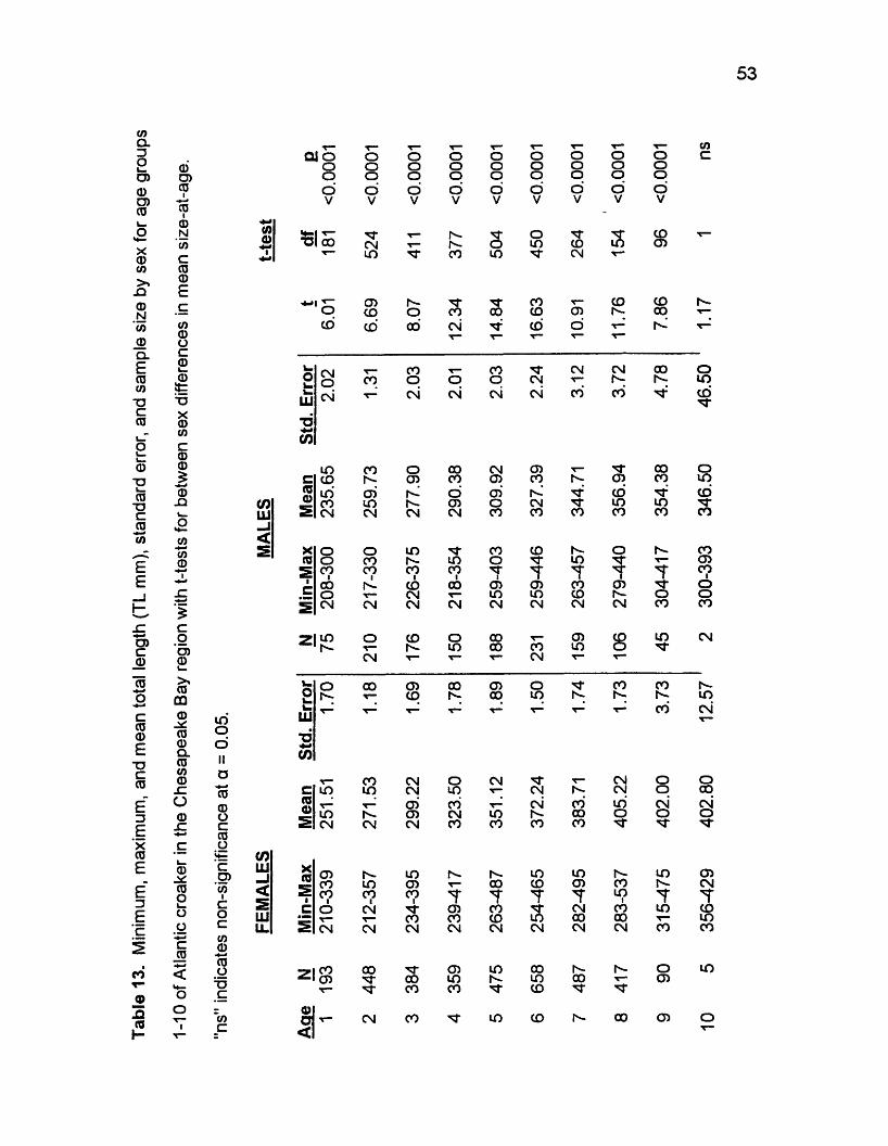
were male. All fish over 457 mm TL were female.

Female and male size compositions were distinctly different within each

year. Females were larger overall, with a mean size of 343 mm TL and a size

range of 210 mm TL to 537 mm TL (pooled Data, Table 9). Males had a mean

size of only 304 mm and a size range of 208 to 457 mm. Both sexes were

smallest in year 1. The mean size of females was 313 mm with a range of 215 to

495 mm then, and the mean size of males was 290 mm with a range of 208 to

457 mm. Both sexes were largest in the year 2. The mean female was 360 mm

with a size range of 210 to 537 mm then, and the mean male was 312 mm with a

45

46

Table 8. Mean, minimum, maximum, Lg95, Lgg, L90, and standard error of mean

total length (TL mm) for Atlantic croaker each year in the Chesapeake Bay region.

Year N Mean Std Error Min Max 1=99.5 1=99 1=90

1 1367 305.72 1.34 208 495 448 439 374

2 2360 348.04 1.25 210 537 468 460 423

3 1132 332.12 1.60 208 474 460 447 403

pooled 4859 332.42 0.85 208 537 464 455 415

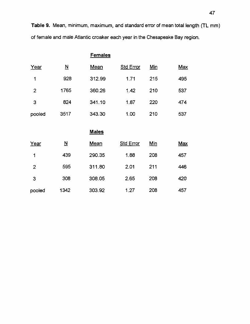
Table 9. Mean, minimum, maximum, and standard error of mean total length (TL mm)

of female and male Atlantic croaker each year in the Chesapeake Bay region.

Females

Year N Mean Std Error Min Max

1 928 312.99 1.71 215 495

2 1765 360.26 1,42 210 537

3 824 341.10 1.87 220 474

pooled 3517 343.30 1.00 210 537

Males

Year N Mean Std Error Min Max

1 439 290.35 1.88 208 457

2 595 311.80 2.01 211 446

3 308 308.05 2.65 208 420

pooled 1342 303.92 1.27 208 457

48

size range of 211 to 446 mm. Females had a mean size of 343 mm in year 3,

with a size range of 220 to 474 mm. Males had a mean size of 308 mm then,

with a size range of 208 mm to 420 mm. There were significant differences in

mean lengths between the sexes in all years (Table 10). Mean sizes were

significantly different between each year for females (ANOVA, F = 215.79, df = 2,

3516, p < 0.0001) and for males (ANOVA, F = 29.71, df = 2, 1341, p < 0.0001).

Length frequency distributions varied between years. The distribution

appeared unimodal in year 1, distributed about the 300 mm interval (Figure 10).

It appeared unimodal but skewed towards larger sizes in year 2, with a peak at

400 mm. The distribution was largely unimodal in year 3, with a peak at 350mm.

KS tests found length frequency distributions were significantly different between

each year (Table 11), but individual length frequencies were not significantly

different from the pooled length frequency distribution.

Size-at-Age

Mean lengths increased with age. Observed mean length increased from

247 mm at age 1 to 387 mm by age 10 (Table 12). The one age 11 fish collected

was 403 mm. Differences between means at age were significant (ANOVA, F =

726.83, df = 9, 4858, p < 0.0001).

Mean lengths-at-age differed by sex. Females were significantly larger at

each age than males except at age 10 (Table 13). Differences between females

and males generally increased from 15.86 mm at age 1 to 47.62 mm at age 9.

Though not significant, the difference between female and male mean size was

56 mm at age 10.

49

Table 10. Unpaired t-tests for differences in mean total lengths (TL mm) of female

and male Atlantic croaker in the Chesapeake Bay region. All results significant at

a = 0.05 with p < 0.0001.

Year t df

1 8.92 1104

2 19.69 1226

3 10.21 630

pooled 24.34 3087

50

Figure 10. Length (TL mm) frequency distributions of Atlantic croaker in the

Chesapeake Bay region each year. Lengths are grouped by .25 mm

size intervals. X-axis values are size interval midpoints, and numbers

above bars represent sample sizes in each interval.

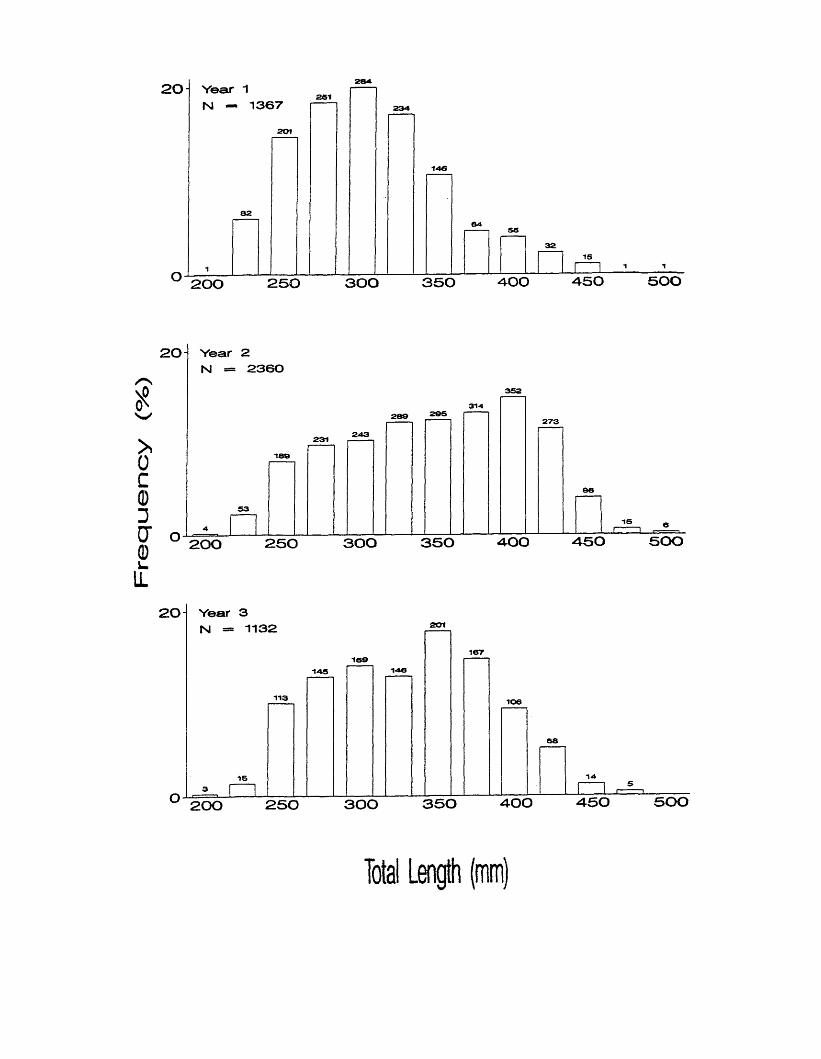
Fre

quency

(%)

2 0 - Year 1 N — 1367

2 0 0 2 5 0 3 0 0 3 5 0 4 0 0 4 5 0 5 0 0

2 0 Year 2 N — 2360

2 0 0 2 5 0 3 0 0 3 5 0 4 0 0 4 5 0 5 0 0

2 0 Year 3 N = 1132

2 0 0 2 5 0 3 0 0 3 5 0 4 0 0 4 5 0 5 0 0

Total Length (mm)

51

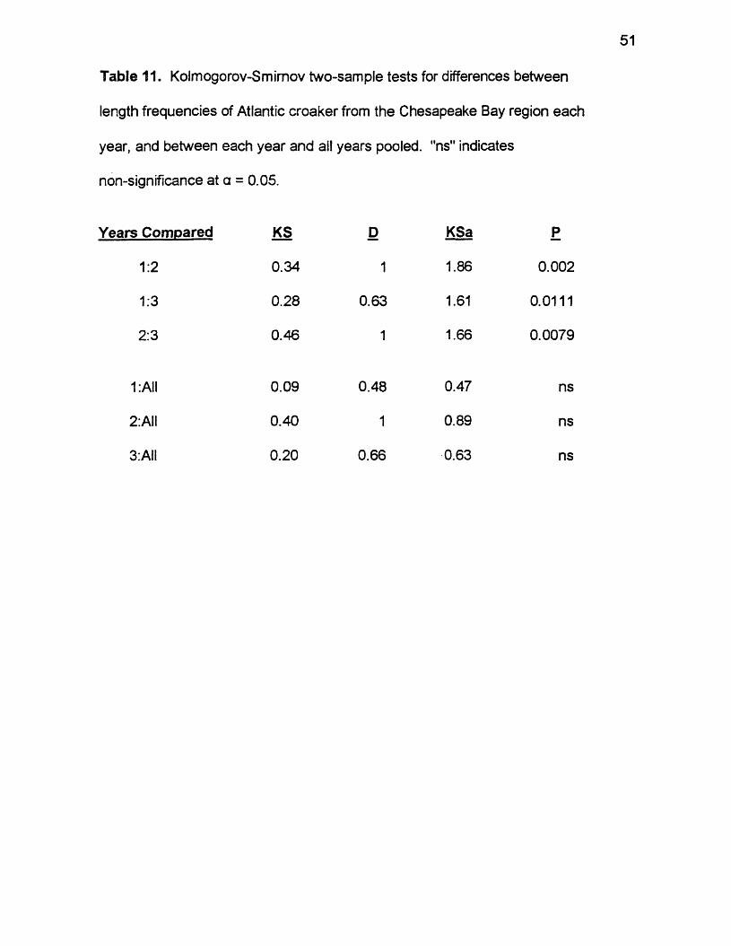
Table 11. Kolmogorov-Smimov two-sample tests for differences between

length frequencies of Atlantic croaker from the Chesapeake Bay region each

year, and between each year and ail years pooled, "ns" indicates

non-significance at a = 0.05.

Years Compared KS D KSa P

1:2 0.34 1 1.86 0.002

1:3 0.28 0.63 1.61 0.0111

2:3 0.46 1 1.66 0.0079

1:AII 0.09 0.48 0.47 ns

2:AII 0.40 1 0.89 ns

3: All 0.20 0.66 0.63 ns

52

Table 12. Observed mean total length (TL mm), 95% confidence limits,

standard error, and sample size for age 1-10 Atlantic croaker in the

Chesapeake Bay region.

Age N Mean TL

1 268 247.07

2 658 267.76

3 560 292.52

4 509 313.74

5 663 339.43

6 889 360.58

7 646 374.11

8 523 395.44

9 135 386.13

10 7 386.71

11 1 403

CL Standard Error

244.29 - 249.86 1.41

265.94 - 269.59 0.93

289.80 - 295.24 1.39

310.72-316.77 1.54

336.21 - 342.66 1.64

357.81 - 363.36 1.41

370.85 - 377.37 1.66

391.93-398.95 1.79

379.16-393.09 3.52

345.33 - 428.09 16.91

Tabl

e 13

. M

inim

um,

max

imum

, an

d m

ean

tota

l len

gth

(TL

mm

), st

anda

rd

erro

r, an

d sa

mpl

e siz

e by

sex

for a

ge

grou

ps

53

0O)COI0t0N</>c00£

V)0Oc0l _0St■DX0(/>C00£0

(A0

QJOOOOV

T5| 00

oCD

<0III

v.ok_u .HI■dCO

CNocsi

oooov

CNin

oooov

ooodv

oooov

oooov

oooov

oooov

T— Is- n- o■X— Is- o m CO m00 m CN

oooov

coCD

mc

6.69

Is-o00 12

.34 00

sr 16.6

3

10.9

1

11.7

6

7.86

T— CO CO CN CN 00CO o o o CN T— Is- Is-T—' csi csi csi csi CO cd

in CO o 00 CN CD T— n- 00CD CD CO CD CO N- CD COin CD o CD h-‘ CDCO in Is- CD O CN n- in inCN CN CN CN CO CO CO CO CO

coCO0

scoO)0i—>*0000-X00CL0CO0

JZO0

0

0OL_ogc0

oo

< .a

inooiia000 c 0 g•+3C,g>CO1cocco00g■oc

COLU

LULL

Ok .k .UJ■dco

o o in N" CO CD r-- o Is-o CO Is- m O sr m N- T “ *

°? CO1

coi

COi T T 'T T00 Is- CD 00 CD CD CO CD ^r

o T— CN T— in m CD r- oCN CN CN CN CN CN CN CN CO

I in o CD O 00 CD 92 inIs- m 00 CO in o 'srCN T“ x—

T _ CN T “ r“o 00 CD 00 CD O CO COIs- T- CD h- 00 in Is- Is- Is-T - ’ T “ v — T - T— T - cd

r— CO CN O CN r̂ T— CN oin m CN in T“ CN Is- CN or— CD CO csi CO in csiin Is- CD CN m r- CO o oCN CN CN CO CO co CO r̂ N-

CD Is- m Is-CO m CDCOI CO1 CO1 "To CN N" CDCO COCN CN CN CN

COCD

r-00TCOCDCN

inCDTsCSI

inCDTCMCOCSI

Is-COinICO00CSI

in

inco

COc

00 CD m 00 N- Is- o00 m Is- m 00 T” CDCO CO N" CD "S’

CN CO m CD Is- 00 CD

m

356-

429

402.

80

12.57

2

300-

393

346.

50

46.50

1.

17

54

Growth

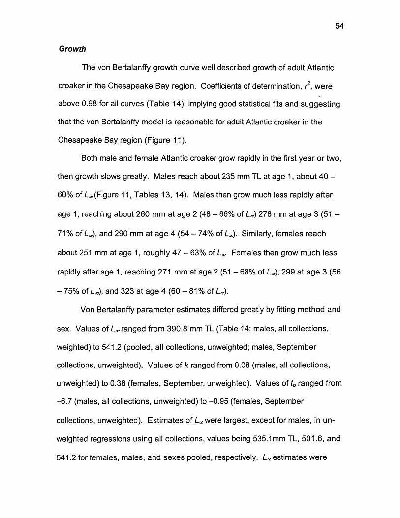
The von Bertalanffy growth curve well described growth of adult Atlantic

croaker in the Chesapeake Bay region. Coefficients of determination, r2, were

above 0.98 for all curves (Table 14), implying good statistical fits and suggesting

that the von Bertalanffy model is reasonable for adult Atlantic croaker in the

Chesapeake Bay region (Figure 11).

Both male and female Atlantic croaker grow rapidly in the first year or two,

then growth slows greatly. Males reach about 235 mm TL at age 1, about 40 -

60% of Leo (Figure 11, Tables 13, 14). Males then grow much less rapidly after

age 1, reaching about 260 mm at age 2 (48 - 66% of Lx) 278 mm at age 3 (51 -

71% of Lao), and 290 mm at age 4 (54 - 74% of LJ. Similarly, females reach

about 251 mm at age 1, roughly 47 - 63% of /.*> Females then grow much less

rapidly after age 1, reaching 271 mm at age 2 (51 - 68% of Lao), 299 at age 3 (56

- 75% of Lao), and 323 at age 4 (60 - 81 % of Lao).

Von Bertalanffy parameter estimates differed greatly by fitting method and

sex. Values of Lao ranged from 390.8 mm TL (Table 14: males, all collections,

weighted) to 541.2 (pooled, all collections, unweighted; males, September

collections, unweighted). Values of k ranged from 0.08 (males, all collections,

unweighted) to 0.38 (females, September, unweighted). Values of t0 ranged from

-6 .7 (males, all collections, unweighted) to -0.95 (females, September

collections, unweighted). Estimates of Lao were largest, except for males, in un­

weighted regressions using all collections, values being 535.1mm TL, 501.6, and

541.2 for females, males, and sexes pooled, respectively. Lao estimates were

55

■ oc0

O

tn0Z0c

00c0

TJU—c8cv-lOO J

tn0N‘0_ 0

CLe00

£

1 0 00E*00i_00e01—0Q l

£

2O)

s0tr0coco>

Q)XI0

h -

0TJO

£0£CDC

c.00c0CLX0

0

00

CO

d )c

c.0’002CD0

00CL> »

00

-Co00

c.00c

Ei—00

T J

o

0c0g

i t0oo

-xi

-11

o l

0<4-̂0

0LJJ

o l

00£0 )LU

o l

00£0

L U

TJ0

g'0

i3

CO CO V - CO O J t oCM r - . CM h - CM

c d c d c s i c d

o

t n

oq

cd

O r - C O T ~ T - O

O O O'

OJ OJ OJOJ OJ OJ

o' o' d

O J h - CMCO X— 'M "CO t o CO■M- CO T —'

0TJo E | O 0 2 Q. LL

t o T— 00 y— O J T TT— CD q CO q

t n in ' cd cd c d

^ r CO X— O J T—

O J co ' c d c d00 r — 0 ’Sf 0i n i n CO ^ r

1

O J cq T - h - "sT

c s i c d 0 ' OO J O J 0 CO CO h -M 1 CO

c m q 0 q 0 0

t r i T - i OJ XT” OCO O CO O Jin m in "M- CO

TJ0

jzg

'0£I

0co

o

00o

c \ i

OJ OJ OJOJ OJ OJ

0 0 d

OJ r^ - CMin00 «n CO

CO X””

0T J —

I ! ! 0

t o CD 10 t o CM CO

o' o' o

N - O J 0 O Jt n 0 xt- T “

c d c d X~

CO M" 00 CO

OJ9

O )COc d

q

CM CO OJ T— CM CO OJx— T“ X~ X— CM CM M"

O d O d O O O|

01

0 0 OJ CO 0 0 "5T in0 0 0 X—x— CM CM

d d d O O O 0 O

CM

o1

00o

d 1

N - OJ 00 00 X—

X— x— T“ CO CO X -

0 d O 0 0 0

0Q l l l 2

TJ0

£g i'0£c310co

o0oou .0JO£0Q0

COc d

q X— 'M’

X— cd CMCM

OJ1CO q T—in OCO CO M -CO CO T “

M ; 0 c m

c d O J XT“

0 O J "c rCO tn

OJ OJ OJOJ OJ OJ

0 0 d

00 t - o h- c o c o x r

0T J —

■s p ® 8 © ®

Q_ LJL «E

56

Figure 11. Observed total lengths-at-age and fitted von Bertalanffy growth

curves by sex for Atlantic croaker in the Chesapeake Bay region. Data points

have been jittered by sex for illustrative purposes.

(lulu) t|}6u a“]

57

smallest, except for males, in unweighted regressions using September

collections, values being 399 mm TL, 541.2, and 403.4 for females, males, and

sexes pooled, respectively. estimates were intermediate for females (441.6

mm TL) and sexes pooled (439 mm) and smallest for males (390.8 mm) in

weighted regressions using all collections. Estimates of k were largest, except

for males, in unweighted regressions using September collections, values being

0.380, 0.107, and 0.342 for females, males, and sexes pooled, respectively, k

estimates were smallest in unweighted regressions using all collections, values

being 0.112, 0.083, and 0.098 for females, males, and sexes pooled,

respectively. Estimates of k were intermediate for females (0.194) and sexes

pooled (0.342) and largest for males (0.178) in weighted regressions using all

collections. Estimates of t0 were largest in un-weighted regressions using

September collections, values being -0.95, -4.02, and -1.19 for females, males,

and sexes pooled, respectively. t0 estimates were smallest in un-weighted

regressions using all collections, values being -4.44, -6.70, and -5.01 for females,

males, and sexes pooled. Estimates of t0 were intermediate in weighted

regressions using all collections, values being -3.09, -4.10, and -3.57 for females,

males, and sexes pooled, respectively.

The significance of between sex differences in von Bertalanffy parameter

estimates varied with regression type. Values of L*, for females (441.6) were

significantly higher than for males (390.8) in weighted regressions using all

collections (Table 15). Female/male differences in L^were not significant in

either un-weighted regressions, all collections or September collections.

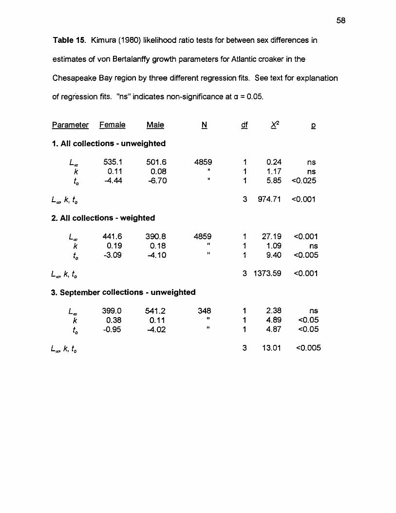
58

Table 15. Kimura (1980) likelihood ratio tests for between sex differences in

estimates of von Bertalanffy growth parameters for Atlantic croaker in the

Chesapeake Bay region by three different regression fits. See text for explanation

of regression fits, "ns" indicates non-significance at a = 0.05.

Parameter Female Male N df x 2 £

1. All collections - unweighted

Lx 535.1 501.6 4859 1 0.24 nsk 0 .1 1 0.08 u 1 1.17 nsto -4.44 -6.70 u

1 5.85 <0.025

k, t0 3 974.71 <0 .0 0 1

2. All collections - weighted

Lm 441.6 390.8 4859 1 27.19 <0 .0 0 1

k 0.19 0.18 it 1 1.09 nst0 -3.09 -4.10 II 1 9.40 <0.005

K t0 3 1373.59 <0 .0 0 1

3. September collections - unweighted

L* 399.0 541.2 348 1 2.38 nsk 0.38 0.11 II 1 4.89 <0.05t0 -0.95 -4.02 II 1 4.87 <0.05

Lc k, t0 3 13.01 <0.005

59

Female/male differences in /cwere significant only in the un-weighted regression

using September collections, for which k was 0.38 in females versus 0.11 in

males. Between sex differences in t0 and the overall curve (all parameters

combined) were significant in all regressions.

Length-Weight

Estimated length-weight relationships were:

TW = 4.2x10'5(TL)2'79 (r2 = 0.99),

TW = 2.3x10'5(TL)2'89 (r2 = 0.99),

TW = 3.1x10‘5(TL)284 (r2 = 0.99),

for females, males, and sexes pooled, respectively. Kimura’s (1980) likelihood

ratio tests found significant differences between the sexes in parameters a, b,

and the overall curve (both parameters combined) (Table 16).

60

Table 16. Kimura (1980) likelihood ratio tests for between sex differences in

total length-total weight relationship parameters. All differences were significant

at a = 0.05, p < 0.001.

Parameter Female Male N df X2

a 4.2x10-5 2.3x10s 4862 1 13.46b 2.79 2.89 4862 1 11.85

a, b 4862 2 89.72

DISCUSSION

Size Composition

The size structure of Atlantic croaker in the Chesapeake Bay region has

changed greatly over the past decade in that much larger fish have been present,

and in large numbers, in recent years. I found a maximum size of 537 mm TL in

contrast to the maximum of 400 mm found by Barbieri (1993). I found 838 fish,

16.9% of my overall collection, as large or larger than the 400 mm maximum that

Barbieri (1993) found. Of my fish, 3 were greater than 500 mm TL. 90% of the

fish I collected were smaller than 415 mm in contrast to the 90% smaller than

295 mm that Barbieri (1993) found. Indeed, 90% of Barbieri’s (1993) fish from

1988 - 1991 were about 40 mm smaller than the overall mean length, 332 mm, I

found from 1998 - 2000. The maximum size that I found, 537 mm, is generally

much larger than those in most other reports outside the Chesapeake Bay region

(417 mm TL - Barger, 1985; 389 mm - Music and Pafford, 1984; 357 mm -

White and Chittenden, 1977). Ross (1988) reported about 100 fish from 400 -

533 mm, the only other study to report many large fish like I found in the 400 -

540 mm size range.

The size structure of Atlantic croaker in the Chesapeake Bay region has

expanded in recent years rather than just shifting towards larger sizes. The size

range that I found, 208 to 537 mm TL, is about 129 mm longer than the size

range of 200 to 400 mm TL that Barbieri et al. (1994a) reported. Because

minimum sizes are similar (208 mm TL in my study, 200 mm in Barbieri et al.

61

62

1994a), the change in size structure appears to reflect a recent expansion into

larger sizes.

Size-at-Age and Growth

I found large between sex differences in size-at-age of Atlantic croaker.

Between sex differences have not been reported in previous studies, most of

which have simply pooled sexes for size and growth analyses (Music and

Pafford, 1984; Barger, 1985; Ross, 1988; Barbieri et al., 1994a). Barger (1985)

and Barbieri et al. (1994a), however, found no between sex differences though

they formally tested for them. Music and Pafford (1984) observed a larger

maximum total length and weight for females, but they did not formally test for

between sex differences.

I found that most Unusually Large Atlantic croaker in the Chesapeake Bay

region are female. This finding is new. Though a few studies have reported very

large Atlantic croaker (Hildebrand and Schroeder, 1928; Massmann and

Pacheco, 1960; Ross, 1988), these studies did not describe the sex composition

of the very large fish.

The von Bertalanffy growth parameter estimates I found generally agree

with previous reports except for that of Ross (1988). Estimates of k (0.36) and t0

(-3.26) found by Barbieri et al. (1994a) fall within the range of values I found for k

(0.08 - 0.38) and t0 (-6.70 - -0.95), though their L^(312.43) falls below the range

I found (390.8 - 541.2). Barger (1985) reported values of 419.2, 0.273, and -

1.405 for k, and t0, respectively, all of which fall within the range of values I

63

found. Ross (1988) reported values of 645, 0.2, and -0.6 for k, and t0,

respectively, of which only k (0 .2 ) falls within the range of values I found.

CHAPTER 3

Mortality

64

INTRODUCTION

Few workers have reported total annual mortality in Atlantic croaker

(White and Chittenden, 1977; Ross, 1988; Barbieri et al., 1994a). White and

Chittenden (1977) targeted Atlantic croaker in the warm temperate waters of the

Gulf of Mexico, but the pertinence of that study to Atlantic croaker farther North is

not clear. Only, Barbieri et al. (1994a) and Ross (1988) have studied Atlantic

croaker total annual mortality in the middle Atlantic region of North Carolina and

the Chesapeake Bay.

Two principal methods have been used to estimate total annual

instantaneous mortality (Z) in Atlantic croaker in the middle Atlantic and

Chesapeake Bay regions. Ross (1988) and Barbieri et al. (1994a) used

regression analysis of catch-curves as described by Chapman and Robson

(1960). White and Chittenden (1977) and Barbieri et al. (1994a) estimated Z

from maximum ages based on negative exponential survivorship as described by

Royce (1972). Barbieri et al. (1994a) also estimated Z based on maximum age

using Hoenig’s (1983) pooled regression equation.

Previous estimates of Z have varied greatly. White and Chittenden (1977)

reported a total annual mortality rate of 96% (Z = 3.2) for Atlantic croaker in the

Northwestern Gulf of Mexico. In contrast, Ross (1988) reported a Z of 1.3 for the

Pamlico Sound area and Barbieri et al. (1994a) obtained estimates for the

Chesapeake Bay region of Z, 0.55, 0.58, and 0.63 using Hoenig’s (1983)

method, Royce’s (1972) method, and regression analysis of a catch-curve,

respectively. It is not clear why these estimates range so widely, but it may be

65

66

due in part to different geographic regions, fishing and natural mortality rates,

and methods of age determination and fish collection. The impacts of large fish

on estimates of total annual mortality are also unclear. Of the previous studies of

mortality in Atlantic croaker, only Ross (1988) collected many fish greater than

400mm total length. However, he used scales and length frequencies to

determine ages, methodologies that have often been questioned in this species

(Roithmayr, 1965; Joseph, 1972; Mericas, 1977; White and Chittenden, 1977;

Barger and Johnson 1980; Jearld, 1983; Barbieri, 1993).

In this chapter, I estimate total annual instantaneous mortality, Z, and

instantaneous natural mortality, M, for adult Atlantic croaker in the Chesapeake

Bay region, and compare these estimates with those of Barbieri (1993), Barbieri

et al. (1994a), and Barbieri et al (1997).

METHODS

Total annual instantaneous mortality

Instantaneous total annual mortality, Z, was estimated from Atlantic

croaker (n=4862) collected in the Chesapeake Bay region and aged using

sectioned otoliths (Chapter 1, Methods). Z, was estimated in three ways: 1)

using Royce’s (1972) method as described by Chittenden and McEachran

(1976), 2) Hoenig’s (1983) method, and 3) by regression analysis of a catch-

curve (Ricker, 1975).

Assuming negative exponential survivorship (Gulland 1969) and following

Royce’s (1972) method for estimating natural mortality in unexploited fish stocks,

Chittenden and McEachran (1976) described a simple equation to estimate Z:

Z = 4.6 / life span,

where life span is the maximum age recorded, and the constant, 4.6, comes from

the expression (In100 - In1), which represents a 99% reduction in the size of an

average year-class from mortality over the fishable life span.

Hoenig (1983) described several equations to estimate Z from maximum

age, based on regression analysis of observed total annual instantaneous

mortality rates on maximum observed ages. I used the predictive equation for all

taxa:

ln(Z) = a + b In ( f max),

where Hoenig gave values of a = 1.44 and b = -0.982, and fmax is the maximum

observed age.

67

68

I estimated maximum age for the Royce (1972) and Hoenig (1983)

methods in three ways: 1 ) as the mean of the three observed maximum ages in

1998, 1999, and 2000, 2) as T99 for ail years pooled, and 3) as the single

maximum observed age over the period 1998 - 2000 (Chapter 1, Table 2).

I used the Adjusted Age Composition (see Chapter 1) to estimate Z via

regression analysis of a catch-curve. The Adjusted Age Composition was based

on pooling all age data from 1998 - 2000 to reduce the effects of variation in

year-class strength (Robson and Chapman, 1961). Following Chapman and

Robson (1960) and Ricker (1975), only recruited age groups containing five or

more fish were used in calculations, and age data were based on collections

from all gear types to minimize sampling bias associated with individual gears.

Finally, following the above guidelines, ages 3 through 10 were used to construct

an initial catch-curve. Catch-curves were also constructed using ages 3 through

9, 2 through 10, and 3 through 9 to evaluate the effects of specific age groups on

estimates of Z.

Z values were converted to S and 1 - S following Ricker (1975).

Instantaneous natural mortality

Instantaneous natural mortality rates, M , were estimated in 4 ways: 1)

using the predictive equation of Alverson and Carney (1975), 2) using Pauly’s

(1980) equation, and 3) using Royce’s (1972) and 4) Hoenig’s (1983) methods

based on maximum age as described by Barbieri (1993).

69

The Alverson and Carney (1975) equation estimates A/f from maximum

age and the Brody growth coefficient of the von Bertalanffy growth equation (see

Ricker, 1975):

fmax x 0.38 = (1//c) x In [ {M+3k) / M ],

where: fmax = maximum fish age (as described above) and k = Brody growth

coefficient. Values of k, and values of Leo for the Pauly (1980) method below,

were based on estimates of these parameters for both sexes pooled (see

Chapter 2).

The Pauly (1980) equation estimates natural mortality from the von

Bertalanffy growth parameter estimates L«, and k, and mean annual water

temperature:

log M = -0.0066 - 0.279 log /.«,+ 0.6543 log k + 0.4634 log 7,

where: Lao- theoretical asymptotic maximum length, k = Brody growth coefficient,

and 7 = mean annual temperature of water inhabited by Atlantic croaker in the

Chesapeake Bay region. Mean temperature estimates were 20.11 C and 19.46

C. Estimates were based on temperature data from March through November,

1998 and 1999, at the ambient condition monitoring station at the Virginia

Institute of Marine Science (2001) and the Virginia Institute of Marine Science,

Juvenile Fish and Blue Crab Trawl Survey (2001), respectively.

Reasoning that Z approximates M when fishing is light or absent,

Barbieri (1993) used Royce’s (1972) and Hoenig’s (1983) methods, as described

earlier, to calculate M based on the maximum age before significant modern

fisheries developed. That maximum age (15 years) was obtained from Hales

70

and Reitz (1992) who aged otolith sections from Indian middens deposited from

1600-1700 A.D. near St. Augustine, FL.

RESULTS

Maximum Age

Estimates of maximum age were generally similar. Maximum age values

were 9 years based on T99 for all years pooled, 10 years based on mean of the

three observed maximum ages in 1998, 1999, and 2000, and 11 years based on

the maximum individual age observed. These values generally agree with

observed maximum age values of 10 and 11 for 1998 - 1999 and 2000,

respectively (see Table 2 in Chapter 1).

Total Annual Mortality and Survivorship

Estimates of total annual mortality and survivorship were generally similar

among maximum age methods. Values of Z ranged from a low of 0.40 to a high

of 0.51 for maximum ages 11 and 9, respectively (Table 17). Values of 1 - S

ranged from 0.33 to 0.40 for maximum ages 11 and 9, respectively, and values of

S ranged from 0.67 to 0.60 for these respective maximum ages.

Estimates of total annual mortality and survivorship based on catch-curve

analysis varied. Estimates of Z ranged from 0.45 to 0.85 (Table 18). Estimates of

1 - S ranged from 0.36 to 0.57, and S ranged from 0.43 to 0.64. The smallest Z

values, 0.45 and 0.46, best statistical fit (r2 = 0.84 and 0.89), and smallest

confidence intervals (0.22 - 0.67, 0.30 - 0.62) were obtained when age 10 was

dropped from the catch-curve. The largest Z values, 0.85 and 0.78, poorest

statistical fit (r2 = 0.67 and 0.70), and widest confidence intervals (0.26 - 1.44,

0.33 - 1.23) were obtained when all fully-recruited ages 3 through 10 plus

71

72

Table 17. Estimates of total annual instantaneous mortality, Z, 1 - S, and S,

based on maximum age methods for listed maximum ages.

Method Max Aae Z 1 -S S

Royce (1972) 9 0.51 0.40 0.6010 0.46 0.37 0.6311 0.42 0.34 0.66

Hoenig (1983) 9 0.49 0.39 0.6110 0.44 0.36 0.6411 0.40 0.33 0.67

73

Table 18. Catch-curve regression estimates of Z, 1 - S, and S, with coefficients

of determination (r2) and 95% confidence intervals (Cl), based on listed ages.

Z J_lS SAaes r2 Estimate Cl ~ Estimate c i Estimate Ci

3 - 1 0 0.67 0.85 0 .26 -1 .44 0.57 0.23 - 0.76 0.43 0.24 - 0.77

3 - 9 0.84 0.45 0.22 - 0.67 0.36 0.20 - 0.49 0.64 0.51 - 0.80

2 - 1 0 0.70 0.78 0 .3 3 -1 .23 0.54 0.28 - 0.71 0.46 0.29 - 0.72

2 - 9 0.89 0.46 0.30 - 0.62 0.37 0.26 - 0.46 0.63 0.54 - 0.74

74

age 2, the peak of the curve, were used (Figure 12). The latter two catch-curves,

however, included an influential observation, age 10, in the calculations.

Abundance at that age was far below the regression line and, as a result, would

greatly affect all regression calculations. Deleting age 10 greatly reduces values

of Z from 0.85 and 0.78 to 0.45 and 0.46, increases i2 from 0.67 and 0.70 to 0.84

and 0.89, and greatly narrows confidence intervals from 0.26 - 1.44 and 0.33 -

1.23 to 0.22 - 0.67 and 0.30 - 0.62.

Instantaneous Natural Mortality, M

Estimates of M ranged from 0.15 to 0.39 with an average of 0.28. The

Alverson and Carney (1975) equation gave estimates ranging from 0.17 to 0.39,

the largest value overall, with an average of 0.29 (Table 19). The Pauly (1980)

equation gave estimates ranging from 0.15, the lowest overall value, to 0.37 with

a mean of 0.26. The Royce (1972) and Hoenig (1983) equations gave similar

values of 0.31 and 0.30, respectively.

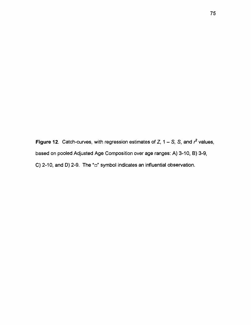
75

Figure 12. Catch-curves, with regression estimates of Z, 1 - S, S, and r2 values,

based on pooled Adjusted Age Composition over age ranges: A) 3-10, B) 3-9,

C) 2-10, and D) 2-9. The symbol indicates an influential observation.

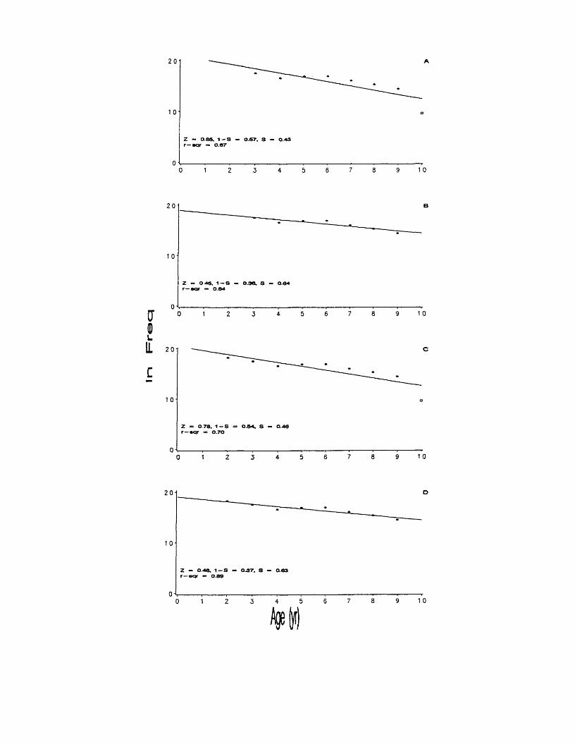
0

0

0.86, 1 -S r - o.er

0.43

01

0

0.64

0 1 2 3 4 5 6 7 8 9 1 0

0 78. 1 — S 0.54. S

17

D

Z - 0.48, 1 -S — 0-37, S - 0.63 r— scjr — 0.83

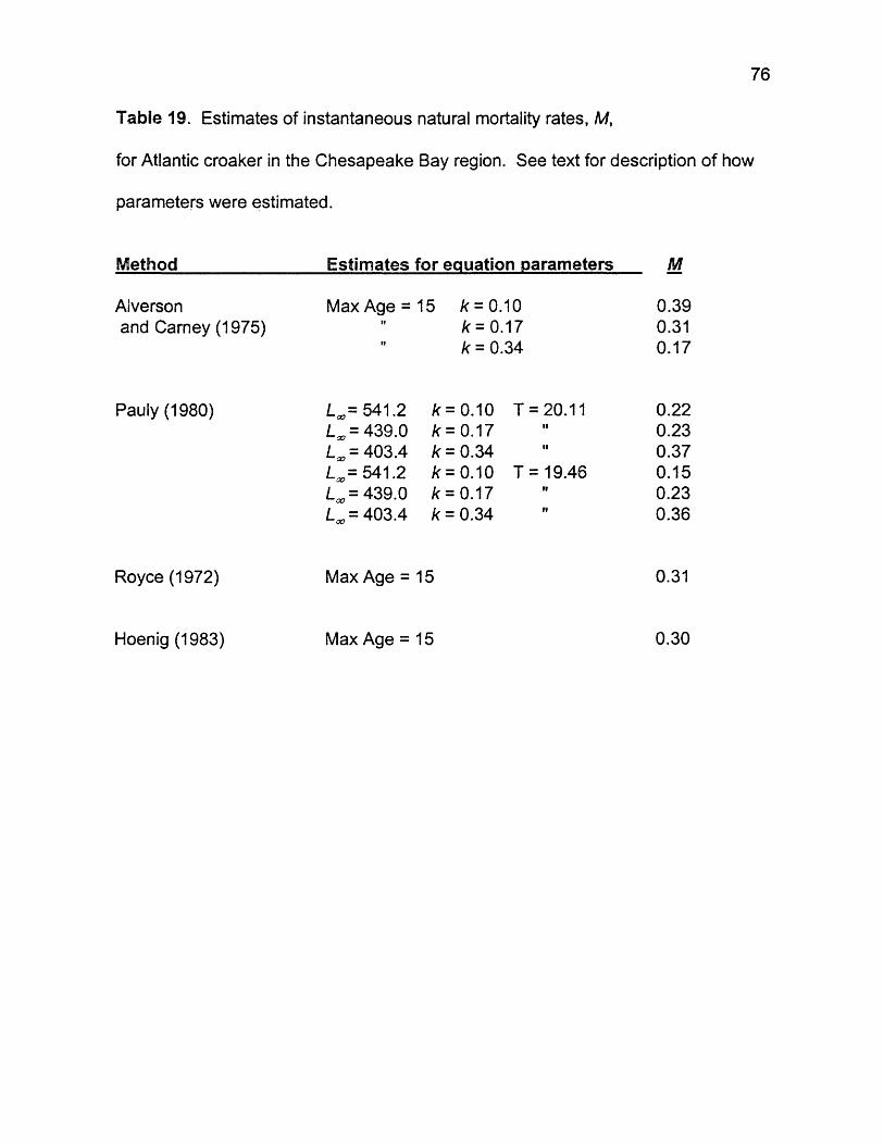
76

Table 19. Estimates of instantaneous natural mortality rates, M,

for Atlantic croaker in the Chesapeake Bay region. See text for description of how

parameters were estimated.

Method_________________Estimates for equation parameters M

Alverson Max Age = 15 /c = 0.10 0.39and Carney (1975) I I k = 0.17 0.31

IS k = 0.34 0.17

Pauly (1980) Lx = 541.2 k = 0.10 T = 20.11 0.22Lao - 439.0 k = 0.17 i f 0.23L ^ - 403.4 k = 0.34 VI 0.37Loo* 541.2 k - 0.10 T = 19.46 0.15Lao = 439.0 k = 0.17 IV 0.23/-«,= 403.4 k = 0.34 i t 0.36

Royce (1972) Max Age = 15 0.31

Hoenig (1983) Max Age = 15 0.30

DISCUSSION

I found that estimates of Z for Atlantic croaker in the Chesapeake Bay

region were 0.40 - 0.51 for maximum age methods and 0.45 to 0.84 for the

catch-curve method. When age 10, an influential observation, is dropped, my

catch-curve estimates, 0.45 and 0.46, agree well with a mid-range value of 0.46

from my maximum age methods, and they indicate 95% confidence limits of 0.22

- 0.67 and 0.30 - 0.62 about Z, respectively. My values of Z from maximum

ages fall just below those of Barbieri et al. (1994a), 0.55 and 0.58. However,

Barbieri et al.’s (1994a) catch-curve estimate of 0.63 falls in the center of my

range of values (0.45 - 0.85) for catch-curves. Both my maximum age and

catch-curve based estimates, as well as those of Barbieri et al. (1994a), fall well

below the catch-curve based estimate, Z = 1.3, reported by Ross (1988) for North

Carolina and the maximum age based estimate of total annual mortality of 96%

(Z = 3.22) reported by White and Chittenden (1977) for the Northwestern Gulf of

Mexico.

I found values for M of 0.15 - 0.39 for Atlantic croaker in the Chesapeake

Bay region. My values calculated using Alverson and Carney (1975) and Pauly

(1980) empirical equations agreed well ranging from 0.17 - 0.39 and 0.15 - 0.36,

respectively. My values based on Royce (1972) and Hoenig (1983) maximum

age methods, as described by Barbieri (1993), were very close (0.31 and 0.30,

respectively) and fell within the range of values I calculated using the empirical

equations. My estimates generally agree well with those of Barbieri (1993), 0.29

77

78

- 0.36, suggesting that these values are reasonable for adult Atlantic croaker in

the Chesapeake Bay region.

LITERATURE CITED

Aiverson, D. L., and M. J. Carney. 1975. A graphic review of the growth and decay of population cohorts. J. Cons. int. Explor. Mer. 36:133-143.

Bagenal, T. B., and F. W. Tesch. 1978. Age and Growth. In: Bagenal TB, editor. Methods for assessment offish production in fresh waters. 3 ed. Oxford: Blackwell Scientific Publications, p 101-136.

Barbieri, L. R. 1993. Life history, population dynamics and yield-per-recruitmodeling of Atlantic croaker, Micropogonias undulatus, in the Chesapeake Bay area PhD Dissertation: College of William and Mary, Williamsburg,VA. 140 p.

Barbieri, L. R., M. E. Chittenden, Jr., and C. M. Jones. 1994a. Age, growth, and mortality of Atlantic croaker, Micropogonias unduiatus, in the Chesapeake Bay region, with a discussion of apparent geographic changes in population dynamics. Fish. Bull. 92:671-685.

Barbieri, L. R., M. E. Chittenden, Jr., and S. K. Lowerre-Barbieri. 1994b. Maturity, spawning, and ovarian cycle of Atlantic croaker, Micropogonias unduiatus, in the Chesapeake Bay and adjacent coastal waters. Fish. Bull. 92:671- 685.

Barbieri, L. R., M. E. Chittenden, Jr., and C. M. Jones. 1997. Yield-per-recruit analysis and management strategies for Atlantic croaker, Micropogonias unduiatus, in the Middle Atlantic Bight. Fish. Bull. 95:637-645.

Barger, L. E. 1985. Age and growth of Atlantic croakers in the northern Gulf of Mexico, based on otolith sections. Trans. Amer. Fish. Soc. 114:847-850.

Barger, L. E., and A. G. Johnson. 1980. An evaluation of hardparts for agedetermination of Atlantic croaker, spot, sandseatrout, and silver seatrout.: NMFS. Report SEFC-22. 5 p.

Beamish, R. J., and G. A. McFariane. 1987. Current trends in age determination methodology. In: R. C. Summerfelt and G. E. Hall, editors. Age and growth offish. Iowa State University Press, Ames, p 15-42.

Bearden, C. M. 1964. Distribution and abundance of Atlantic croaker,Micropogonias unduiatus, in South Carolina. Contrib. Bears Bluff. Lab. 40, 23 p.

Cerrato, R. M. 1990. Interpretable statistical tests for growth comparisons using parameters in the von Bertalanffy equation. Can. J. Fish. Aquat. Sci. 47:1416-1426.

79

80

Chao, L. N. 1978. Family : Sciaenidae. Micropogonias unduiatus. In: Fischer W., editor. FAO species identification sheets for fishery purposes, western central Atlantic: fishing area 31. Rome: FAO. p [unpaged].

Chao, L. N., and J. A. Musick. 1977. Life history, feeding habits, and functional morphology of juvenile sciaenid fishes in the York River estuary, Virginia. Fish. Bull. 75:657-702.

Chapman, D. G., and D. S. Robson. 1960. The analysis of a catch curve. Biometrics 16:354-368.

Chittenden, M. E., Jr. 1989. Sources of variation in Chesapeake Bay pound-net and haul-seine catch compositions. N. Amer. J. Fish. Mgmt. 9:367-371.

Chittenden, M. E., Jr., and J. D. McEachran. 1976. Composition, ecology, and dynamics of demersal fish communities on the northwestern Gulf of Mexico continental shelf, with a similar synopsis for the entire Gulf. Tex. A&M Univ., Sea Grant Publ. No. TAMU-SG-76-208. 104 p.

Christmas, J. Y., and R. S. Waller. 1973. Estuarine vertebrates, Mississippi. In: Christmas, J. Y., editor. Cooperative Gulf of Mexico estuarine inventory and study, Mississippi. Gulf Coast Res. Lab. p 320-434.

Cochran, W. G. 1977. Sampling techniques. John Wiley and Sons, New York. 428 p.

Colton, J. B., Jr., W. G. Smith, A. W. Kendall, Jr., P. L. Berrien, and M. P. Fahay. 1979. Principal spawning areas and times of marine fishes, Cape Sable to Cape Hatteras. Fish. Bull. 76:911-915.

Diagnostic Instruments, Inc. 1997. SPOT RT. Version 3.0.4: Diagnostic Instruments, Inc.

Gallaway, B. J., and K. Strawn. 1974. Seasonal abundance and distribution of marine fishes at a hot-water discharge in Galveston Bay, Texas. Contrib. Mar. Sci. Univ. Tex. 18:71-137.

Gulland, J. A. 1969. Manual of methods for fish stock assessment. Part I. Fish population analysis. Rome: FAO. Report 4. 154 p.

Gunter, G. 1945. Studies on marine fishes of Texas. Publ. Inst. Mar. Sci. Univ. Texas 1:1-190.

81

Hales, L. S., Jr., and E. J. Reitz. 1992. Historical changes in age and growth of Atlantic croaker, Micropogonias unduiatus (Perciformes: Sciaenidae). J. Archaeolog. Sci. 19:73-99.

Hansen, D. J. 1969. Food, growth, migration, reproduction, and abundance of pinfish, Lagodon rhomboides, and Atlantic croaker, Micropogonias unduiatus, near Pensacola, Florida, 1963-65. U. S. Fish Wildl. Serv., Fish. Bull. 68:135-146.

Haven, D. S. 1954. Croakers. Va. Comm. Fish. 54th and 55th Annu. Rep. 1952- 1953, p. 49-53.

Haven, D. S. 1957. Distribution, growth, and availability of juvenile croaker, Micropogonias unduiatus, in Virginia. Ecology 38:88-97.

Haven, D. S. 1959. Migration of the croaker, Micropooonias unduiatus. Copeia 1959:25-30.

Hildebrand, S. F., and L. E. Cable. 1930. Development and life history of fourteen teleostean fishes at Beaufort, N.C. Bull. U. S. Bur. Fish. 46:384-488.

Hildebrand, S. F., and W. C. Schroeder. 1928. Fishes of the Chesapeake Bay. Bull. U. S. Bur. Fish. 43:1-366.

Hoenig, J. M. 1983. Empirical use of longevity data to estimate mortality rates. Fish. Bull. 82:898-902.

Hoese, H. D. 1973. A trawl survey of nearshore fishes and invertebrates of the Georgia coast. Contrib. Mar. Sci. Univ. Tex. 17:63-98.

Jearld, A. J. 1983. Age determination. In: L. A. Nielsen and D. L. Johnson,editors. Fisheries techniques. American Fisheries Society, Bethesda, MD. p 301-324.

Joseph, E. B. 1972. The status of the sciaenid stocks of the middle Atlantic coast. Ches. Sci. 13:87-100.

Kimura, D. K. 1980. Likelihood methods for the von Bertalanffy growth curve.Fish. Bull. 77:765-776.

Laird, A. K., S. A. Tyler, and A. D. Barton. 1965. Dynamics of normal growth. Growth 29:233-248.

Massmann, W. H. and A. L. Pacheco. 1960. Disappearance of young Atlanticcroaker from the York River, Virginia. Trans. Amer. Fish. Soc. 89:154-159.

82

Mericas, C. E. 1977. The eye lens weight technique in aging of the Atlantic croaker, Micropogonias unduiatus. Gulf Res. Rep. 6:71-73.

Morse, W. W. 1980. Maturity, spawning and fecundity of Atlantic croaker, Micropogonias unduiatus. occurring north of Cape Hatteras, North Carolina. Fish. Bull. 78:190-195.

Music, J. L., Jr., and J. M. Pafford. 1984. Population dynamics and life history aspects of major marine sportfishes in Georgia's coastal waters. Georgia Dep. Nat. Resourc., Coastal Resourc. Div., Contr. Ser. No. 38, Brunswick, 382 p.

Nixon, S. W., and C. M. Jones. 1997. Age and growth of larval and juvenileAtlantic croaker, Micropogonias unduiatus, from the Middle Atlantic Bight and estuarine waters of Virginia. Fish. Bull. 95:773-784.

Norcross, B. L. 1983. Climate scale environmental factors affecting year-class fluctuations of Atlantic croaker (Micropogonias unduiatus) in the Chesapeake Bay, Virginia, PhD Dissertation: School of Marine Science, College of William and Mary, Williamsburg, VA. 388 p.

Norcross, B. L., and H. M. Austin. 1988. Middle Atlantic Bight meridional windcomponent effect on bottom water temperatures and spawning distribution of Atlantic croaker. Cont. Shelf Res. 8:69-88.

Pauly, D. 1980. On the relationships between natural mortality, growthparameters, and mean environmental temperature in 175 fish stocks. J. Cons. int. Explor. Mer. 39:175-192.

Ricker, W. E. 1975. Computation and interpretation of biological statistics offish populations. Bull. Fish. Res. Board. Can 191. 382 p.

Robson, D. S., and D. G. Chapman. 1961. Catch curves and mortality rates. Trans. Amer. Fish. Soc. 90:181-189.

Roithmayr, C. M. 1965. Review of industrial bottomfish fishery in northern Gulf of Mexico, 1959-62. Comm. Fish. Rev., U. S. 27:1-6.

Ross, S. W. 1988. Age, growth, and mortality of Atlantic croaker in NorthCarolina, with comments on population dynamics. Trans. Amer. Fish. Soc. 117:461-473.

Rothschild, B. J., P. W. Jones, and J. S. Wilson. 1981. Trends in Chesapeake Bay fisheries. Trans. 46th N. Amer. Wildl. Nat. Resour. Conf.:284-298.

83

Royce, W. F. 1972. Introduction to the fisheries sciences. Academic Press, New York. 351 p.

SAS Institute, Inc. 1999. SAS/STAT@ User'sGuide, Version 7-1. SAS Institute Inc, Cary, NC. 3365 p.

Suttkus, R. D. 1955. Seasonal movements and growth of the Atlantic croaker (Micropogonias unduiatus) along the east Louisiana coast. Proc. Gulf Caribb. Fish. Inst. 7: 151-158.

Virginia Institute of Marine Science. March, 2001.York River Ambient Monitoring Data.VIMS Scientific Data Archive (http://www.vims.edu/data_archive).Va. Institute of Marine Science, School of Marine Science,College of William & Mary. Gloucester Pt., VA.

Virginia Institute of Marine Science, Juvenile Fish and Blue Crab Trawl Survey. March, 2001. Data Archive (http://www.fisheries.vims.edu/vimstrawldata) Va. Institute of Marine Science, School of Marine Science,College of William & Mary. Gloucester Pt., VA.

von Bertalanffy, L. 1938. A quantitative theory of organic growth. II. Inquiries on growth laws. Human Biology 10:181-213.

von Bertalanffy, L. 1957. Quantitative laws in metabolism and growth. Quarterly Review of Biology 32:217-231.

Wallace, D. H. 1940. Sexual development of the croaker, Micropogoniasunduiatus, and distribution of the early stages in Chesapeake Bay. Trans. Amer. Fish. Soc. 70:475-482.

Warlen, S. M. 1982. Age and growth of larvae and spawning time of Atlantic croaker in North Carolina. Proc. Ann. Conf. S. E. Assoc. Fish. Wildl. Agencies 34:204-214.

Warlen, S. M., and J. S. Burke. 1991. Immigration of larvae of fall/winterspawning marine fishes into a North Carolina estuary. Estuaries 13:453- 461.

Welsh, W. W., and C. M. Breder. 1923. Contributions to the life histories of Sciaenidae of the eastern United States coast. Bull. U. S. Bur. Fish. 39:141-201.

White, M. L., and M. E. Chittenden, Jr. 1977. Age determination, reproduction, and population dynamics of the Atlantic croaker, Micropogonias unduiatus. Fish. Bull. 75:109-123.

84

Zar, J. H.. 1984. Biostatistical Analysis. Prentice-Hall, Englewood Cliffs, NJ. 718 P-

VITA

John Richard Foster

Bom in Dallas, Texas, 05 August 1975. Entered Texas A & M University,

Galveston in 1993. Earned B.S., cum laude, with a double major in Marine Biology and

Marine Fisheries in 1997. Entered masters program in Marine Science at the College of

William and Mary, School of Marine Science, Virginia Institute of Marine Science in

1997. Began working as an analytical fisheries scientist for the Georgia Department of

Natural Resources, Coastal Resources Division, Marine Fisheries Section in January

2001. Defended his thesis on 12 June 2001.

85