AFWAL-TR-86-4024

A USER'S GUIDE TO THE PICKER DIFFRACTOMETER FOR POLYMERMORPHOLOGY STUDIES

P. Galen LenhertPhysics DepartmentVanderbilt UniversityNashville, Tennessee 37235

Joseph F. O'Brien and W. Wade AdamsPolymer BranchNonmetallic Materials Division

December 1986

Interim Report for Period 1980 - 1984

Approved for Public Resease; Distribution Unlimited

Best Available Copy

MATERIALS LABORATORYAIR FORCE WRIGHT AERONAUTICAL LABORATORIESAIR FORCE SYSTEMS COMMANDWRIGHT-PATTERSON AIR FORCE BASE, OHIO 45433-6533

NOTICE

When Government drawings, specifications, or other data are usedfor any purpose other than in connection with a definitely relatedGovernment procurement operation, the United States Government therebyincurs no responsibility nor any obligation whatsoever; and the factthat the Government may have formulated, furnished, or in any waysupplied the said drawings, specifications, or other data, is not to beregarded by implication or otherwise as in any manner licensing theholder or any other person or corporation, or conveying any rights orpermission to manufacture use, or sell any patented invention that mayin any way be related thereto.

This report has been reviewed by the Office of Public Affairs(ASD/PA) and is releasable to the National Technical Information Service(NTIS). At NTIS, it will be available to the general public, includingforeign nationals.

This technical report has been reviewed and is approved forpublication.

IZ/1

1• / / ~-1 ,6l

THADDEUS E. hEtMINIAK RICHARD L. VAN DEUSENProject Engineer Chief, Polymer Branch

FOR THE COMMANDER

"-'MERRILL L. MINGES, PhD, SESDirectorNonmetallic Materials Division

"If your address has changed,'if you wish to be removed from our mailing

list, or if the addressee is no longer employed by your organizationplease notify AFWAL/MLBP, Wright-Patterson AFB OH 45433 to help usmaintain a current mailing list."

Copies of this report should not be returned unless return is requiredby security considerations, contractual obligations, or notice on aspecific document.

UnclassifiedSECURITY CLASSIFICATION OF THIS PAGE

REPORT DOCUMENTATION PAGE

is. REPORT SECURITY CLASSIFICATION lb. RESTRICTIVE MARKINGS

Unclassified2a. SECURITY CLASSIFICATION AUTHORITY 3. DISTRIBUTION/AVAILABILITY OF REPORT

Approved for public release;2b. DECLASSIFICATION/DOWNGRADING SCHEDULE distribution is unlimited

4. PERFORMING ORGANIZATION REPORT NUMBER(S) 5. MONITORING ORGANIZATION REPORT NUMBER(S)

AFWAL-TR-86-40246a. NAME OF PERFORMING ORGANIZATION 6b. OFFICE SYMBOL 7a. NAME OF MONITORING ORGANIZATION

(If applicable)

Materials Laboratory AFWAL/MLBP

6c. ADDRESS (City. State and ZIP Code) 7b. ADDRESS (City, State and ZIP Code)

Wright-Patterson Air Force BaseOhio 45433-6533

ga. NAME OF FUNDING/SPONSORING 8b. OFFICE SYMBOL 9. PROCUREMENT INSTRUMENT IDENTIFICATION NUMBERORGANIZATION (If applicable)

Se. ADDRESS (City, State and ZIP Code) 10. SOURCE OF FUNDING NOS.

PROGRAM PROJECT TASK WORK UNITELEMENT NO. NO. NO. NO.

11. TITLE (Include Security Classification)

A User's Guide to the Picker Diffractometer 61102F 2303 Q3 0712. PERSONAL AUTHOR(S)

P. G. Lenhert. J. F. O'Brien and W. W. Adams13& TYPE OF REPORT 13b. TIME COVERED 14. DATE OF REPORT (Yr., Mo., Day) 15. PAGE COUNT

FROM 1980 TO 1984 mber 1986 48

16. SUPPLEMENTARY NOTATION

17. COSATI CODES 18. SUBJECT TERMS (Continue on reverse if necessary and identify by block number)

FIELD GROUP SUB. GR. X-ray Diffraction Polymer Morphology Crystallite Size07 04 X-ray Diffractometer Orientation Pole Figure1I 09

19. ABSTRACT (Continue on reverse if necessary and identify by block number)

The use of the Picker Automated Four-Circle X-Ray Diffractometer System for PolymerMorphology studies is explained and illustrated. Operations of the instrument, selectionof experimental parameters, and specific methods for the following analyses arepresented: crystallite size, orientation factors (with resolved or overlappedreflections), layer line intensity scan, and full pole figures.

20. DISTRIBUTION/AVAILABILITY OF ABSTRACT 21. ABSTRACT SECURITY CLASSIFICATION

UNCLASSIFIED/UNLIMITED IN SAME AS RPT. El DTIC USERS Unclassified

22a. NAME OF RESPONSIBLE INDIVIDUAL 22b. TELEPHONE NUMBER 22c. OFFICE SYMBOL(Include Area Code)

Dr. W. W. Adams 513-255-2340 AFWAL/MLBP

DD FORM 1473, 83 APR EDITION OF 1 JAN 73 IS OBSOLETE. nclass ieSECURITY CLASSIFICATION OF THIS PAGE

i

UnclassifiedSECURITY CLASSIFICATION OF THIS PAGE

11. for Polymer Morphology Studies

Unclassifiedii SECURITY CLASSIFICATION OF THIS PAGE

FOREWORD

This report was prepared by the Polymer Branch, Nonmetallic MaterialsDivision, and Vanderbilt University (through Universal Energy Systems, Inc.)

under contract F33615-82-C-5001 to the Materials Laboratory. The work wasinitiated under Project 2302, "Research to Define the Structure PropertyRelationships," Task No. 2303Q3, Work Unit Directive 2303Q307, "StructuralResins." Dr Thaddeus E. Helminiak served as the AFWAL/ML Work UnitScientist. Co-authors were Dr P. Galen Lenhert, Vanderbilt University, andLt Joseph F. O'Brien and Dr W. Wade Adams, Materials Laboratory (AFWAL/MLBP).This report covers research conducted from 1980-1984.

iii

TABLE OF CONTENTS

SECTION PAGE

I INTRODUCTION 1

II GENERAL COMMENTS ON THE PICKER FACS-I SYSTEM 2

III CHOICE OF INSTRUMENTAL PARAMETERS 4

IV CRYSTALLITE SIZE DETERMINATION IN POLYMER SAMPLES 6

V ORIENTATION FACTOR MEASUREMENTS: RESOLVED PEAKS 23

VI DETERMINATION OF ORIENTATION FOR POLYMER FIBERS:OVERLAPPING REFLECTIONS 28

VII DIFFRACTOMETER SCANS ALONG LAYER LINES FOR POLYMERMATERIALS 30

VIII POLE FIGURE DATA COLLECTION AND ANALYSIS 34

REFERENCES 41

v ,

LIST OF FIGURES

FIGURE NO. PAGE

1 HMTA in 0.5 mm Capillary as Crystallized. 7

2 HMTA Recrystallized and Ground.

(a) 0.27 mm Capillary Exposed 8 hours 8

(b) 0.5 mm Capillary Exposed 1 Hour 8

3 Plot of the HMTA Data in Table 1. 10

4 Graph of ABPBI-PBT Blend Equatorial Scan. 19

5 Plots of Full Width at Half Maximum (in Units of 2sinS)Standards.

(a) Equatorial Geometry, Sample Diameter vs As forReflections at 17.850 and 31.200 20. 20

(b) Meridional Geometry, s vs As, Data for 0.29 mm

and 0.54 mm Capillaries. 21

6 Plot of First Layer Line for ABPBT Fibers. 33

7 Pole Figure Geometry, Reflection and Transmission Methods. 34

vi

LIST OF TABLES

TABLE NO. PAGE

1 TWO-THETA, SCAN OF MMTA FACS-I INPUT AND OUTPUT 9

2 PEAK FIT OF THE DATA IN TABLE 1 12

3 TWO-THETA SCAN OF HEAT-TREATED ABPBI-PBT FIBERS 15

4 EXAMPLE PRINTOUT CHECK FOR TAIL OF A PBO DISTRIBUTION 24

5 EXAMPLE ORIENTATION FACTOR RUN FOR PBO (AS-SPUN)#042083N1 25

6 ORIENTATION FACTORS FOR TWO PBT REFLECTIONS 26

7 ORIENTATION FACTORS FOR VARIOUS SVA HEIGHTS 26

8 PRECISION OF ORIENTATION FACTOR 27

9 EXAMPLE OF FACS-I INPUT-OUTPUT FOR A LAYER LINE SCANFOR A HEAT-TREATED ABPBT SAMPLE 32

10 EXAMPLE OF TAPE HEADING 35

11 TRANSMISSION MODE POLE FIGURE INPUT AND OUTPUT 36

12 TWO-THETA SCAN FOR A BUNDLE OF PBT FIBERS 37

13 UNIAXIAL SCANS FOR PBT 38

14 UNIAXIAL SCAN FOR PBT WITH BACKGROUNDS MEASURED FOR20 S EACH, 1.30 ABOVE AND BELOW THE PEAK POSITION 38

vii

SECTION I

INTRODUCTION

The Picker FACS-I automated x-ray diffractometer has been an integral part of

the Polymer Branch Morphology Laboratory since 1975, when it was moved from

the Metals Division to its present home in the Nonmetallic Division inBuilding 56,. Although designed originally fpr use solely as a single-crystal

diffractometer, it has been used extensively in the Polymer Branch MorphologyLaboratory for polymer analysis. Modifications to the control software on

the PDP 8/1 computer have enabled the scientist to collect data onsemi-crystalline or amorphous polymer specimens, in order to studycrystallite orientation and crystallite size, shapes of amorphous halos, andintensity distributions for polymer structure analysis.

This report provides essential information for use of the Picker system for

polymer analysis. It is not intended to be all inclusive; as moreexperiments are performed, modification will be necessary. In addition, asthe equipment is updated, the manual will be revised accordingly.

SECTION II

GENERAL COMMENTS ON THE PICKER FACS-I SYSTEM

The FACS-I automated diffractometer was designed to collect x-ray diffractiondata for single-crystal structure analysis. It can also be used to makediffraction measurements on polycrystalline materials for orientationstudies, crystallite size determination or for two-dimensional pole figureanalysis. In general the instrument parameters are similar for both types ofexperiments. The sample, sample holder and measurement procedures differ.

The instrument consists of a PDP 8/1 computer which is interfaced to thegoniostat (diffractometer), the x-ray tube shutter and the diffracted beamfilter wheels. The computer controls each of the four goniostat angles(26, w, X, and 4) by means of a motor used to drive the angle and an encoderwhich reads the angle positions to 0.01*. The control program acceptscommands which are converted by the computer to appropriate electricalsignals and sent to the hardware. Commands are entered into the computerthrough the terminal keyboard. As discussed below, simple commands alloweach hardware function to be activated individually. Other commands causethe computer to carry out complex functions such as the various datacollection modes.

The x-ray tube is independent of the computer and operates continuously atvoltage and current settings selected manually. The x-ray beam from the tubecan be "reflected" from a monochromator crystal, allowed to pass directly tothe sample or filtered by an appropriate beta filter. An incident beamcollimator allows a narrow beam of x-rays to fall on the sample. X-raysscattered (diffracted) by the sample are detected when they enter thediffracted beam collimator and fall on the detector surface. This collimatorserves mainly to keep radiation scattered by the air from entering thedetector. The angular resolution of the instrument is determined by thex-ray source size, the area (or volume) of the sample illuminated, and thedetector aperture (SVA) which can be varied symmetrically in both verticaland horizontal width.

X-ray quanta that enter the detector produce electrical pulses which areamplified by a preamplifier connected directly to the photomultiplier tube inthe detector. These pulses are sent to the pulse height analyzer and, ifthey pass the energy discrimination criteria which have been set manually,are counted by the scaler. The scaler unit also contains a digital clock(timer). Both the scaler and the timer can be started, stopped and read bythe PDP 8/1 computer.

The use of the computer and the diffractometer control programs are discussedin the manual for the Vanderbilt Disl-Oriented Diffractometer System (Lenhert,1974). The manual should be consulted (and studied) before using thecomputer. The elementary commands allow manipulation of individual angles,shutter, timer, scaler, etc. Other commands are used to carry out scans,execute a series of pole figure measurements, write the results on magnetic,etc.

2

X-ray tubes designed for diffraction usually have molybdenum or coppertargets. The Ka line is prominent for both materials. In some experimentsthe full spectrum of the tube is used, but more often a filter is inserted topartially remove the unwanted portion of the spectrum. If a high degree ofmonochromaticity is required a monochromator crystal must be used.Documentation supplied with the x-ray tube will show the operational limitsof the tube in use. The standard operating voltage for Mo tubes is 50 Kv.Cu tubes are usually run at 30 to 40 Kv. Tube design and focal spot sizedetermine the maximum loading and, therefore, the highest current settingallowed.

3

SECTION III

CHOICE OF INSTRUMENTAL PARAMETERS

GONIOSTAT ALIGNMENT

Alignment of the x-ray tube and the four-circle goniostat is an exacting taskand should be undertaken only by one very experienced in the use of theFACS-I system. Alignment procedure and hints are described by Lenhert(1978). If, after studying the alignment procedure you feel alignment isneeded, and believe you are competent to undertake the task, go ahead onlyafter obtaining permission from the person responsible for thediffractometer.

ANALYZER SETTINGS

Before making any x-ray measurements, the analyzer settings should bechecked. They should be set to accept 90% to 95% of the counts at thewavelength to be used for the experiment, usually Mo Y or Cu Ka. Theanalyzer should reject all counts which differ from this wavelength by morethan 30% to 40%. Rejection is better for the shorter wavelength, i.e., Mo Ka.

Analyzer settings which will provide a usable band pass are 100% window, gainat 10, upper rejection level at 7.0, lower rejection level at 4.0. For Mo K0,the high voltage (detector voltage) should be set to 5.20 (1 Kv or a littlemore). The high-voltage settings will need to be adjusted if you change to adifferent radiation. It must also be checked at least once a month; sincethe Nal(Th) crystal-photomultiplier detector ages, the setting will have tobe adjusted. It should be checked before any major experiment.

The correct high-voltage setting may be determined by obtaining amonochromatic beam from a single crystal or the monochromator. (CAUTION: Ifyou use the monochromator,be sure the SVA is closed far enough to preventdamage to the detector, since the beam stop must be removed and the detectorwill be subjected to the direct beam from the monochromator.) With theshutter open and the monochromatic beam directed at the detector, check thecount rate at various high-voltage settings. Adjust the high voltage formaximum count rate.)

With the analyzer set as described, the normal background and.system noisewill give about one count per minute (CPM) with x-rays ON and the shutterclosed. If you get more than 1 CPM you probably have a hardware problem.

MONOCHROMATOR

To insert the monochroviator, remove the monochromator housing cover, slidethe monochromator "boat" into place, tighten the screw and replace the cover.Next set the two monochromator angles, 20 and P to the values recorded inSmonothe FACS-I Log Book. You should now have a strong uniform monochromatic beamwhen the shutter is opened. The beam uniformity may be conveniently checkedby using a pinhole aperture mounted on a sample holder and placed in thex-ray beam. If the pinhole is offset and the X circle is rotated, the beamintensity can be checked on a circular locus of points. For details seeLenhert (1980).

4

DIFFRACTOMETER PARAMETERS

The effective source size, collimator size, sample size and shape, and thediffracted beam aperture must be optimized for best results. The choice ofthese parameters determines the intensity of the diffracted beam and theresolution of the experiment. Increased resolution is usually obtained atthe expense of intensity, so a compromise must be reached which will give theresolution required without excessive counting times. Each experiment hasits own requirements but general rules are helpful, and in many casesstandard settings may be used.

The rule with fewest exceptions applies to collimator size. For general usewith both single crystals and polycrystalline materials, use the 1.0collimators. The incident beam and diffracted beam collimators are notinterchangeable! The collimator with circular grooves goes on the diffractedbeam side.

The effective x-ray source is adjusted by changing the x-ray tubetake-off-angle (TOA). High-resolution experiments require a small sourcesize which is obtained with a small TOA. For cell constant determinationswith single crystals one might use a TOA of 1.00. Single crystal datacollection is normally done with TOA settings of 2.50 to 3.5*. Polymermaterials usually give more diffuse diffraction patterns and TOA settings of3.0* to 4.0* are normal settings.

The diffracted beam aperture is determined by the setting of thesymmetrically variable aperture (SVA). Small settings are used when highresolution is required. Data for use in calculating single-crystal cellconstants may be taken with SVA settings of 1.0mm vertical opening and 1.0mmhorizontal width. Single crystal data collection is normally done with anSVA setting of 3.75mm x 3.75mm. Experiments with polycrystalline materialssometimes require resolution only with respect to 2e. For such experimentsthe SVA should be set wide open in the vertical direction. If resolution isrequired (for example with pole figure or orientation measurements) thevertical SVA opening will usually be restricted to a range of 2mm to 4mm. Asimilar range will usually be satisfactory for horizontal SVA settings when 2eresolution is important to the experiment.

The optimum sample size is often set by the form of the material available.If the experiment requires that the entire sample must be illuminated by thex-ray beam then the sample must have a maximum dimension no greater than1.0mm. Fiber samples should have a cross section of 1mm or less but theeffective sample size along the fiber bundle will be determined by thedimensions of the beam. Samples in the form of sheets will extend beyond thebeam in two directions and will have an effective size determined by thex-ray beam cross section.

In many experiments choice of diffraction parameters will be critical. Thesecases are discussed in the following sections devoted to the different typesof measurements.

5

SECTION IV

CRYSTALLITE SIZE DETERMINATION IN POLYMER SAMPLES

Bragg diffraction peaks have a finite width due to the finite size of thecrystallites giving rise to the diffraction pattern. However, this is onlyone of several reasons why Bragg reflections are, in practice, not ofinfinitesimal width. Lattice distortions of various sorts along withinstrumental factors and sample size all increase the breadth of Bragg peaksfor a real sample measured on a diffractometer with finite x-ray source andaperture.

PREPARATION AND USE OF HEXAMINE STANDARDS

The usual method of correcting for instrumental factors is to use a standardsubstance with large enough crystallite size to remove this cause of linebroadening. In our study, hexamethylenetetramine (HMTA) from Aldrich wasrecrystallized by Mr Al Sicree. HMTA is somewhat hygroscopic and therecrystallized material of July 14, 1982 is stored in a desiccator undervacuum. It should be pumped to restore the vacuum immediately after removinga sample.

The crystallites in the recrystallized material are much too large to give auniform powder pattern. The photograph, figure 1, made from ungroundrecrystallized material shows this. If unground material is used on thediffractometer to make theta scans the peak contains fine structure due toindividual crystallites. The peak shapes are therefore not an accuratereflection of the instrumental and sample size parameters and should not beused to correct polymer diffraction scans for these factors.

6

Figure 1. HMTA in 0.5 mm Capillary as Crystallized. Cu Ka, Ni filter,30 Kv, 20 ma.

Experience shows that HMTA powder satisfactory for use as a standard can beobtained by grinding the recrystallized material with a mortar and pestle.Be careful not to try to grind too much material at one time. It takes verylittle to fill a capillary tube. Grind it for 30 minutes or so taking careto work over all parts of the batch you are grinding. Scrape it off thesides of the mortar every few minutes to be sure it is evenly ground.

Fill the capillary tubes by introducing a small amount in the open end andworking it to the bottom by stroking the top of the tube with a file to makethe tube vibrate and by poking it carefully down the tube with a small tubeor a glass fiber. When the bottom 1 to 2 cm of the tube is filled, use thesmall glass burner and seal the open end. You will find this easy to do ifyou pull on both ends of the capillary as you put it into the flame.Complete the seal by heating the tip of the sample tube to form a small bead.Mount the sample tube (which should be about 2 to 3 cm long) in one of thesmall aluminum sample holders. Finally, mount it on a goniometer head.

A photograph taken with the precession camera (no precession motion) shouldshow no more structure than those in figure 2. Samples of 0.27 mm, 0.5 mmand 0.7 mm have been prepared and their powder diagrams measured on thediffractometer.

7

(a) 0.27 mm capillary exposed 8 hours (b) 0.5 mm capillary exposed I hour

Figure 2. HMTA Recrystallized and Ground. Capillary horizontal inprecession camera (no precession motion). Prepared August 2,1982, Cu Ka Ni filter 30 Kv 20 ma.

Sample size is one of the parameters that determines the broadening of apowder line. Therefore, to correct for sample size, one must use a standardsample the same size as the polymer sample being investigated. Consider alsothat the effective sample size is equal to the actual sample size only if thesample is smaller than the x-ray beam. If the sample is horizontal (as witha meridional scan) the effective sample size in the direction of interestwill be determined by the width of the x-ray beam. Therefore a scan at X= 0must be made for use with equatorial scans and one at X = 90 (capillaryhorizontal) for use with meridionalreflections.

The quality of the scans obtained with the standards was greatly improved bygrinding the HMTA but continuous rotation of the sample (the phi angle on theFACS-I) improved them further. Phi rotation is obtained by setting the PDP8/I switch registers to 7776 when the scans are started. Use the /TH commandof DIFF, write the data on magnetic tape, enter it into the off-site computervia NFRATINI and plot and analyze it in the usual way. Be sure that you makeyour scans with fine enough 28 steps in the region of the peaks you intend touse. Be sure to count long enough to get good counting statistics i.e.,1000 + counts for the peaks and at least 200 - 300 counts for all points onthe scan.

The following input (Table 1) was used to obtain satisfactory scans with oursamples prepared as described above. Figure 3 shows a plot of the data intable 1.

8

TABLE 1. TWO-THETA SCAN OF HMTA FACS-I INPUT AND OUTPUT

/DC90/PT8/FM/HDHEXASTD3 .5MM CAPILLARY MERIDIONAL SCAN/TH

TH=14 DLTH=.5 TH=16 DLTH=.05 TH=19 DLTH=.5 TH=29DLTH=.05 TH=32.5 DLTH=.5 TH=43 DLTH=.05 TH=46 DLTH=.5 TH=50DLTH=O

1.90 1.91 2.06 2.10 2.38 2.38 2.31 2.56 2.27 2.452.40 2.42 2.36 2.39 2.48 2.29 2.32 2.24 2.38 2.462.28 2.59 2.74 2.77 3.09 3.16 3.52 3.91 4.35 7.16

12.49 21.88 32.19 42.74 53.05 63.23 72.10 80.56 91.51 101.47106.23 107.73 105.65 101.15 90.63 80.59 72.94 62.33 53.11 43.4031.97 20.57 11.30 6.08 4.64 4.58 4.10 3.97 4.04 4.484.15 4.05 4.18 4.38 4.09 3.78 3.15 2.92 2.94 2.742.85 3.05 2.74 2.95 3.02 2.79 4.79 5.80 3.00 2.852.83 2.81 2.96 2.63 2.81 2.58 2.62 2.78 2.97 2.792.82 2.86 2.78 2.63 2.53 2.71 2.74 2.89 2.72 2.872.53 2.97 2.80 2.59 2.68 2.62 2.61 2.85 2.82 2.672.88 2.81 3.06 2.90 3.32 3.34 3.96 4.86 6.20 7.059.05 11.10 13.17 14.50 15.37 16.92 17.67 18.27 17.86 17.81

16.40 14.63 13.03 11.58 10.56 9.05 7.06 5.41 4.11 3.353.14 2.84 2.91 2.76 2.88 2.63 2.68 2.83 2.70 2.592.61 2.81 2.62 2.76 2.69 2.45 2.48 2.46 2.15 2.192.11 4.11 3.32 1.98 1.92 2.04 1.88 1.82 1.96 2.092.09 2.07 1.90 1.94 1.93 2.61 2.39 2.45 2.41 2.212.40 2.52 2.38 2.35 2.32 2.30 2.28 2.16 2.00 2.102.12 2.23 2.18 2.32 2.26 2.26 2.54 3.03 3.28 3.904.65 4.85 5.88 6.61 7.27 8.17 9.00 9.91 9.79 9.649.69 9.29 8.12 7.90 7.36 6.11 5.45 4.45 3.43 2.812.59 2.24 2.19 2.16 2.09 2.18 2.04 1.90 2.01 2.052.00 2.13 1.79 2.03 2.05 2.15 2.07 1.75 1.75 3.307.12 2.62 1.80 1.92

9

HEXASTO3 .5MM CAPILLARY MERIDIONAL SCAN

C..

NO COMMNO8 BMWNO SRPN

I-.

'-4z

6. .A 15.'k.;. 35.66 4.i@ 45.66.56.6 55.0

TWO THETA

Figure 3. Plot of the HMTA Data in Table 1. Intensity in counts per second.Cu Ka with graphite monochromator.

10

DETERMINATION OF THE INSTRUMENTAL BROADENING PARAMETER WITH HMTA STANDARDS

Measurement conditions previously used for polymer samples (SVA located 230mm from the sample, open to 3 x 3 mm and a tube TOA of 3.00) were found togive diffraction peaks with flat tops with HMTA because the intrinsic widthof the HMTA Peaks was smaller than the extended, uniform x-ray source. Itwas subsequently found that an x-ray tube TOA of 1.00 (1 cm actual focal. spotlength) which corresponds to an angular width of about 0.040, and an SVAwidth of 0.5 mm, which corresponds to an angular width of about 0.120, gavepeaks which could be fit with Gaussian profiles using an available computerprogram (Anderson, 1985). The following example (table 2) shows the inputand output of the peak fit program using the data in table 1. The scan ismade with Cu Ka monochromatized radiation and a 2e step size varying from0.50 in the background region to 0.050 in the peak region. Fits can beobtained with peak step sizes of 0.050 but ease of fit is increased ifsmaller steps are used in the peak region.

- 1

TABLE 2. PEAK FIT OF*THE DATA TN TABLE 1. LOW ANGLE PEAK ONLY.

fYPE THE NUMBER OF PEAKS AND DASELINE POINTSEG 3 (MAXIMUM OF 6 FOR EACH)12

;YPE THE POSITIONS OF THE BASELINE THEN INTENSITIES1 FIXES THE PARAMETER 0 DOES NOT EG:1.222 2.333 3.444 4.5550 11.222 0 22.333 1 33.444 1 44.555

.16932 .225251 2.0 1 3.0

PEAK P0S INT AT MAX HALF-WIDTH GAUSS1 2.12345 1 30.12345 0 0.12345 0 0.12 FOR EXAMPLE

0 .220123 100.0 0 .005 0 .25YOU HAVE MADE AN ERROR TYPING IN THE FITTING PARAMETERS, RETYPE THE LINE YOU JUST TYPED.0 .20123 0 100.0 0 .005 0 .25

:: HMTA 0.54MM CAPILLARY MERIDIONAL SCAN

WEIGHT FACTOR=I/Y(I)

FOR ITERATION >1 SE = 0.693623E-05FOR ITERATION > 2 SE = 0.115529E-05FOR ITERATION > 3 SE = 0.788330E-06FOR ITERATION > 4 SE = 0.787355E-06FOR ITERATION > 5 SE = 0.787345E-06

THE AREAS UNDER THE VARIOUS PEAKS ARE GIVEN BELOW:AREAS 0.83448INTEGRAL BREADTH 0.00724BASELINE AREA = 0.13984

FINAL FITTING PARAMETERS USED

PEAK POS INT AT MAX HALF-WIDTH GAUSS0 0.20123 0 115.21251 0 0.00680 1 1.00

BASELINE POSITIONS AND INTENSITIES0.1693 1 2.000000.2253 1 3.00000DO YOU WANT A PRINT-OUT OF THE FITTED DATA;YES

12

TABLE 2 CONTINUED

INDIVIDUALTWO ++++ INTENSITIES +-i-+ PEAKSTHETA S(I/A) OBSERVED CALCULATED OBS-CALC BASELINE PK I

15.00 0.1693 2.140 2.000 0.140 2.000 0.00015.50 0.1749 2.187 2.100 0.087 2.100 0.00016.00 0.1805 2.485 2.201 0.284 2.201 0.000

17.55 0.1979 66.597 61.596 5.001 2.511 59.08517.60 0.1985 75.961 75.046 0.915 2.521 72.52517.65 0.1990 84.899 88.282 -3.382 2.531 85.75117.70 0.1996 96.468 100.199 -3.731 2.541 97.65817.75 0.2001 106.999 109.679 -2.680 2.551 107.12817.80 0.2007 112.052 115.757 -3.705 2.561 113.19617.85 0.2012 113.668 117.781 -4.114 2.571 115.21117.90 0.2018 111.507 115.533 -4.026 2.581 112.95217.95 0.2024 106.789 109.259 -2.470 2.591 106.66918.00 0.2029 95.711 99.634 -3.922 2.601 97.03318.05 0.2035 85.134 87.638 -2.503 2.611 85.02718.10 0.2040 77.076 74.391 2.685 2.621 71.770

19.00 0.2141 4.346 2.806 1.540 2.801 0.00619.50 0.2197 4.030 2.900 1.129 2.900 0.00020.00 0.2253 3.369 3.000 0.369 3.000 0.000

13

Similar scans were made for cylindrical samples which measured 0.54 and 0.69mm in diameter. The reflections at 17.850 and 31.200 were scanned for allsamples. The full width at half maximum (FWHM) was obtained by computer fitand plotted versus sample diameter for each reflection. For these samplesthe FWHM represents the instrumental broadening as a function of sample sizebecause the crystallite size is large. Values for sample sizes in the rangefrom 0.25 mm to 0.70 mm can be read from the curves. Since FWHM is afunction of 20, one must interpolate for reflections at other diffractionangles.

Equatorial scans of fiber bundles of polymer materials were made and allpeaks in the region of interest (00 to 400 2e) were fit. The followingexample, table 3, shows a scan with 4 peaks and the calculation of peakparameters for a similar scan. FWHM in units of 2sin0 /X are tabulated. Theresults of the curve fit are shown in figure 4. Crystallite size wascalculated from the relations:

Ag2 = A - Aln2

t obs 'inst

and

Kt

where AU is the FWHM due to crystallite size, Ao is the FWHM observed andAýs5. is the FWHM due to instrumental factors (as betermined from the HMTAscans.L then gives the crystallite size in 9 when the constant K (unity inour case) is divided by Aý . The results are plotted in figure 5 for bothequatorial and meridional geometry.

Note that the effective sample size will change for a given sample when onegoes from the equatorial orientation to the meridional orientation where thex-ray beam diameter rather than the sample itself effectively defines thesample size.

14

TABLE 3. TWO-THETA SCAN OF HEAT-TREATED ABPBI-PBT FIBERS INCLUDING PEAKS AT11.16, 14.40 AND 26.00 FOLLOWED BY PEAK PARAMETERS FROMLEAST-SQUARES FIT.

/FM

/PT8

/TH

TH=3 DLTH=.5 TH=8 DLTH-.2 TH=33 DLTH-.5 TH=40 DLTH=O

24.78 15.10 11.01 8.99 7.95 7.39 7.07 7.23 7.16 7.45

8.83 9.29 10.08 10.20 11.74 12.76 13.84 15.87 17.48 20.43

23.48 26.69 31.67 36.63 41.73 46.10 51.11 53.66 54.80 53.80

51.39 47.41 42.75 39.17 35.27 33.63 31.82 30.91 30.58 30.24

31.00 30.88 31.60 31.42 31.07 30.56 29.76 29.00 27.22 25.86

24.74 24.06 22.70 21.97 21.18 20.05 20.16 18.81 19.65 18.71

18.93 19.13 19.22 18.72 19.01 19.43 19.59 19.29 19.62 20.74

20.57 20.86 21.33 21.80 22.63 23.58 24.52 24.56 25.74 27.03

28.38 29.05 30.65 32.24 34.16 37.18 39.13 42.33 45.88 50.65

54.42 62.02 67.23 76.49 84.55 93.95 102.36 112.26 119.14 125.04

125.43 123.94 117.22 108.28 98.28 87.32 75.09 66.58 56.63 49.57

42.77 38.30 34.33 29.18 26.14 23.77 21.94 19.75 18.35 17.09

15.63 13.94 12.93 12.13 11.16 10.51 9.54 9.18 8.52 8.23

7.59 7.24 6.59 6.46 6.14 6.08 5.18 5.09 4.72 4.35

4.14 3.92 3.91 3.51 3.65 3.76 3.59 3.58 3.54 3.54

15

TABLE 3 CONTINUED

DO YOU ANT TO FIT THIS DATA,YES

WEI8&T FACTOR?@--SORT (Y (I) IYMAX)1=!/Y (I)

FRVý WHAT INITIAL S TO WHAT FINAL S8.87 Lo"THE MIN S IS AT 8. 6789 THIS IS THE 7 DATA POINTTHE MAX S IS AT 0.44366 THIS IS THE 158 DATA POINT

THE TOTAL NU11BER OF DATA POINTS TO BE FITTED IS 144THE AVERAGE S IS 8. 24343 AND THE AVERAGE RCI IS 34.35187

TYPE HE NU'BER OF PEAAS AND BASELINE POINTSEG 3 (MAXiMUK OF 6 FOR EACH)42

TYPE THE POSITIONS OF THE BASELINE THEN INTENSITIESi FIXES THE PARAM ETER 0 DOES NOT EG:1.2 2.333 3.444 4.555t !1.22 0 L.333 1 33.444 1 44.555

0.06789 0.44366.5.0 1 2.0

PEAK PUS INT AT .MX HALF-WIDTH GAUSS1 2.12345 1 30.12345 0 0.12345 6 8.12 FOR EXAMPLE

S.13 0 45.0 8 .05 0 .5

0 .17 0 20.0 0 .@5 0 .50 .28 0 3@.80 8.85 @ .50 .30 0 58.@ 8 .85 0 .5

, ABPBI-PBT HT EGUATORIAL SCAN... CHI=I, DEGREES CU T

WEIGHT FACTOR - 1/Y(I)

FOR ITERATION ) 1 SE = 0.695056E-05FOR ITERATION ) 2 SE = 0.222054E-05FOR ITERATION ) 3 SE = 0.101181E-05

FOR ITERATION ) 27 SE = 0.684118E-07FOR ITERATION ) 28 SE - 0.678114E-07FOR ITERATION ) 29 SE - 0.672242E-07FQOE ITERATION ) 30 SE - 0.666495E-07THE AREAS UNDER THE VARIOUS EAKS ARE GIVEN BELOW:RES = 1.21395 2.55963 3.58372 3.7649

iNTESRAL BReaDTh= .03t78 0. 13@9 1. 18572" @. 13610BASELINE IREA = .9394

, PA.ETERS USED

*."- K '4NT T YI~ ',ýA.:-W]17Ti EJSS1 A 48 L K47 @l,65

35!ý , S33. 896SE6 K Il 432 e; 8.54S8, 7 8 i4.27425 • •..BE! I 8l.61

BP SEUJ Z OI~ AND " IS7IT ES5. eg679 3, 886t. 4437 2. Zilloo

THIS WPS "H: *!XIMUi ITERATION BUT IT HS NOT YETCONVERGED. DO YOU WANT TO TRY AGAIN;Nc BEST AVAILABLE COPYDO YOU WPNT ýA PRINT-OUT OF ThE FI7ED DATA;YES 16

TABLE 3 CONTINUED

TWO S-I/) ++I+ iNTENSiT!ES ++*+ INDIVIDUAL PEAKSTHT,, OBSERVED CALCIJULTED OBS-CALC BASELINE PK I PK 2 PK 3 P"K 46.20 0.0679 7.113 6.821 0.292 3.000 0.536 s.5r1 0.559 0. i65

6.50 0.0735 7.282 7.243 t.039 2.985 0.645 2.85. 0.589 0.1737.00 0.0792 7.22L 7.753 -0.533 2.970 0.789 3.I9M 0.621 0.1837.50 0.0848 7.521 8.382 -0.860 2.955 0.988 3.590 0.656 , .1938. W 0. @9F5 8.724 9.189 -0.465 2.94@ 1.287 4.065 0.694 0.2048,.2 0.0927 9.396 9.591 -0.195 2.934 1.459 4.280 0.710 0.2088.40 0.095? 10.201 1..064 0.137 2.928 1.686 4.510 Z.727 0.2138.60 8,0973 10.328 10.637 -0.309 2.922 1.995 4.759 0.744 0.2188.80 0.2995 11.895 11.357 @.538 2.916 2.430 5.026 M.762 0.2239.08 0.1018 12.936 12.288 0.648 2.910 3.054 5.315 0.780 0.2289.2@ 0.1,04 !..040 13.515 0.524 2.904 3.951 5.627 @.799 0.2343.40 8@.'63 16.109 15143 0.966 2.898 5.222 5.964 Z.819 0.240Io6 ? 0,.85 17.755 ,7.285 0.468 2.892 6.98i 6.328 0.840 2.2459.80 0.1;08 20.764 28.053 0.711 2.886 9.332 6.723 0.861 0.25210,00 0.1f3! 23.880 23.522 0.359 2.880 12.350 7.151 0.884 0.258i0. 8 0.2153 27.164 27.78 -0.544 2.874 16.048 7.614 0.907 0.2644.40 0.1176 32.254 32.538 -9.284 2.868 2@.351 8.117 0.931 0.271,0.60 0.11!98 37.332 37,822 -0.489 2.862 25.064 8.662 0.956 0.278A.80 @.i221 42.561 43.229 -0.668 2.856 29.853 9.253 0.981 0.28611.88 ?1,243 47.052 48,278 -1.226 2.850 34.234 9.892 1.089 0.29311.210 .1266 52.205 52.359 -0.154 2.844 37.593 10.584 1.037 0.30111.40 @.1288 54.851 54,857 -0.086 2.838 39.313 11.331 1.866 0.31011.60, .1311 56.060 55.397 0.663 2.832 39.015 12.135 1.@97 0.31811.88 8.1333 55.881 54.849 1.832 2.826 36.770 12.996 1.1,9 0.32712. W 0.1356 52.655 51.289 1.367 2.82M 33.053 13.916 1.163 0.33712.20 @.1378 48.617 47.752 0.865 2.814 28.582 14.891 1.198 @.347.2.48 0.1401 43.875 44.015 -0.140 2.808 23.699 15.916 1.235 0.35712.60 0.1423 40.234 40,509 -0.274 2.802 19.083 16.982 1.274 0.368:2.80 0.1446 36.259 37.511 -1.252 2.796 14.945 18.077 1.315 @.37913.00 8.1468 34.604 35.162 -8.558 2.790 11.442 19.181 1.358 0.39113.20 0.1491 32.770 33.485 -0.715 2.784 8.621 20.273 1.404 0.403i3.40 0.1513 31.861 32.417 -0.556 2.778 6.448 21.322 1.453 0.41613.6e 0.1536 31.550 31.841 -0.291 2.772 4.838 22.297 1.505 0.42913.80 0.1558 31.228 31.611 -0.383 2.766 3.682 23.159 -.560 0.44314.88 L.I581 32.843 31.581 0.462 2.760 2.870 23.874 1.619 0.45814.20 0.1603 31.949 31.621 0.328 2.754 2.304 24.407 1.683 0.47414.4@ 0.1626 32.725 31.628 1.097 2.748 1.907 24.731 '.751 0.49014.6R 0.1648 32.571 31.527 !.@43 2.742 1.624 24.829 1.825 0.507:4.80 0.1671 32.240 31.276 8.94 2.736 1.414 24.696 i.9F5 8.52515.@ 0..1693 31.742 38.857 0.885 2.730 1.252 24,.338 1, 92 054515028 8.1716 30.943 30.274 0.669 2.724 1.-23 23.776 2.087 8.,515.4@ 0.1738 30.183 29.547 0.637 2.718 1.015 23.037 2.190 0.58615.68 W .176M 28.368 28.705 -0.345 2.712 @.924 22.157 2.304 0.60915.80 0.1783 2S.972 27.784 -0.812 2.706 0.845 21.172 2.428 0.63216.00 0.1805 25.831 26.816 -,.985 2.700 0.776 20.118 2.565 0.65816.28 0. 1828 25. 148 25.836 -0.688 2.694 0.715 19.026 2.716 0.684_6.40 2.,85@ 23.753 24.87? -1.!!8 2.688 0.661 17.926 2.882 f.71316.60 0.!873 23.:14 23.943 -0.929 2.682 0.613 16.839 3.866 0.74316.80 8 . i895 L).212 23.073 -0.861 2.676 0.569 15.782 3.269 0.77517.00 0.1917 21.?50 22.272 -1.222 2.670 0.531 14.769 3.493 0.81017.20 e,1940 21.190 2!.552 -0.362 2.664 0.496 13.806 3.740 0.84617.4@ 0.1962 19.794 20.919 -1.125 2.659 0.464 12.898 4.013 0.885:7,R, 081984 20.702 24.376 8.326 2.653 0.435 12.048 4.314 0.92717.88 0.67 19.735 19.928 -.192 2.647 8,489 11.256 4.644 0.972

8.00 0.2029 19.991 19.574 @.418 2.641 @.385 10.528 5.688 1.02n18.20 0.2052 20.227 19.314 @.9!3 2.635 0.363 9.838 5.487 1.7218.41 08.24 28.347 '9.15@ 1.197 2.629 0.343 9.207 5.843 1.128i8.60 0.2896 19.842 19.080 0.762 2.623 0.325 8.625 6.320 1.188:8.80 0.2119 2R.175 19.183 1.072 2.617 0.308 8.88 6.838 1.253J9.0, 0.2141 20.647 19.219 1.427 2.611 0.292 7.592 7.401 1.3239. 20 0.2163 20.843 19.427 1.416 2.685 @.277 7.135 8.011 1.400!9.48 0.2186 20.551 19.726 0.824 2.599 0.264 6.712 8.668 1.483.9.60 082288 20.929 20.115 08.14 2.593 @.251 6.323 9.375 1K5731•.80 0.223e 22.153 20.594 c.559 2.587 0.240 5.962 10.132 1.673L M 0. 2253 22. 001 2!,.161 0.840 2.581 0.229 5.629 10.940 1.781

N.2 0. 2275 22.341 21.815 0.526 2.575 0.219 5.321 11.799 1.90020. " & 2297 22.875 22.555 0.320 2.569 0.209 5.835 12.709 2.032,n, 6 @.2319 23.411 23.380 0.031 2.563 0,208 4.771 13.669 2.177'1.80 Z.2342 24.336 24.288 ?.@48 2.558 0.192 4.525 14.676 2.338"z8 8 2364 25.393 25.'79 8,1i5 2.552 0.184 4.296 15.729 2.518

BEST AVAILABLE COPY

-17

TABLE 3 CONCLUDED

2 0.' ýM o.2386 26.443 26.349 0. 93 2.546 0.177 4.?83 16.82 4 2.72,21.4Q 0.2488 26.523 27.500 -0.976 2.548 0.170 3.885 17.956 2.94821.60 0.2431 27.837 28.72q -0.892 2.534 0.163 3.700 19.122 3.2102. 8@ 0.2453 29.275 30.041 -0.767 2.528 0.157 3.527 20.315 3.51422.80 0.2475 30.782 31.441 -0.659 2.522 @.151 3.366 21.528 3.87422.2n 0.2497 31.555 32.940 -1.386 2.516 8.146 3.215 22.752 4.31122.48 8.2528 33.342 34.561 -1.219 2.51 @ 0.141 3.073 23.978 4.85822.6 9.2542 35.124 36.336 -1.212 2.504 0.136 2.941 25.196 5.56022.8? 0.2364 37.272 38.320 -1.048 2.498 0.131 2.816 26.392 6.48323.8M 0.2586 40.629 40.588 0.041 2.492 8.127 2.699 27.553 7.71723.20 0.2608 42-.825 43.242 -0.417 2.487 0.123 2.589 28.665 9.37923.40 0.263! 46.399 46.410 -0.011 2.481 0.119 2.485 29.712 11.61423.E 0.2653 50.368 5@.243 0.125 2.475 0.115 2.387 30,677 14.58923.80 0.2675 55.692 54.902 0.790 2.469 0.111 2.295 31.544 18.48324.8N 0.2697 59.932 60.540 -0.608 2.463 0.108 2.2f7 32.296 23.46624.20 @.2719 68.411 67.274 1.137 2.457 0.104 2.125 32.918 29.67024.48 t.2741 74.277 75.155 -0.877 2.451 8.101 2.047 33.395 37.16@24.60 0.2763 84.645 84.133 0.512 2.445 0.098 1.973 33.718 45.89824.80 0.2785 93.717 94.027 -@.309 2.439 0.895 1.903 33.879 55.718K.8O 0.2808 104.308 104.489 -0.181 2.434 0.093 1.836 33.873 66.25425.20 0.283@ 113.834 114.981 -1.148 2.428 8.098 1.773 33.782 76.98925.4@ 0.2852 125.052 124.745 0.307 2.422 0.087 1.713 33.369 87.15425.60 0.2874 132.939 132.816 0.123 2.416 0.085 1.656 32.882 95.77725.88 0.28% 139.759 138.129 1.630 2.418 0.083 1.602 32.254 181.78026. 0 0.2918 140,434 139.777 8.657 2.404 0.088 1.550 31.498 184.24426.20 0.2940 139.085 137.351 1.654 2.398 0.078 1.501 30.630 102.74426.40 0.2962 131.6% 131.136 0.559 2.392 0.076 1.454 6.665 97.54826.60 0.2984 121.864 121.984 -8.128 2.387 8.074 1. 489 28. 622 89.49226.8e 0.30@6 110.804 118.977 -0.173 2.381 8.872 1.367 27.515 79.64227.00 0.3028 98.621 99.140 -0.519 2.375 0.071 1.326 26.361 69. M827.20 0. 305e 84.959 87.30f -2.341 2.369 0.069 1.287 25.175 58.40127.40 0.3072 75.466 76. 055 -0.589 2.363 0.067 1.249 23.968 48.40727.6( 0.3094 64.304 65.801 -1.497 2.357 0.0866 1.213 22.754 39.41127.88 0.3116 56.389 56.759 -0.370 2.351 0.064 1.179 21.543 31.62228.8 08.3138 48.743 49.006 -0.263 2.346 0.062 1.146 28.344 25.10828.20 0.316@ 43.729 42.508 1.221 2.340 0.861 1.115 19.165 19.82728.40 0.3!82 39.269 37.154 2.115 2.334 0.860 1.084 18.013 15.663"28.68 0.3284 33.448 32.792 0.649 2.328 0.858 1.855 16.894 12.45628.80 0.3226 30.013 29.250 0.763 2.32 0.057 1.027 15.812 10.03129.00 0.3248 27.343 26.364 0.980 2.316 0.056 1.881 14.772 8.21929.220 0.3270 25.286 23.986 1.308 2.311 0.854 0.975 13.776 6.87129.40 0.3292 22.86 21.998 8.808 2.305 0.053 0.950 12.827 5.86329.6S 0.3314 21.230 20.303 8.927 2.299 0.052 0.926 11.927 5.0992W.88 0.3335 19.810 18.831 0.979 2.293 0.051 0.903 11.875 4.50930.0 0..3357 18.153 17.532 ?.621 2.287 0.050 0.881 10.274 4.0403K.20 0.3379 16.222 16.369 -0.147 2.281 0.049 8.860 9.522 3.65730,4Z 0.3401 15.876 15.319 -0.243 2.276 0.848 0.839 8.820 3.33738,68 0.3423 14.172 14.364 -0.192 2.270 0.047 0.819 8.165 3.086330.80 0.3445 13.064 13.492 -0.428 2.264 0.046 0.8@@ 7.558 2.82531.88 U.3467 12.328 12.695 -0.367 2.258 0.045 0.782 6.995 2.6153. 0.3488 ".013 11.964 -0.752 2.252 @.@44 0.764 6.476 2.42831.40 0.3510 18.812 11.296 -0.484 2.247 0.043 0.747 5.998 2.26131.60 0.3532 !el.055 1.683 -0.628 2.241 0.042 0.730 5.559 2.11131. 8? t.3554 9.733 10.123 -0.390 2.235 0.042 0.714 5.158 l.97532MOO 0.3575 8.994 9.61@ -0.616 2.229 0.041 0.698 4.790 1.85232.28 0.3597 8.597 9.141 -0.544 2.223 0.040 8.683 4.455 1.73932.42 0.3619 7.842 8.712 -@.871 2.218 0.039 0.669 4.150 1.63732.60 0.3641 7.703 8.321 -0.617 2.212 0.039 0.655 3.872 1.54332.80 @.3662 7.337 7.962 -0.625 2.206 0.038 0.641 3.628 1.45733.8 0.3684 7.281 7.634 -@.354 2.208 0.037 0.628 3.391 1.37933.58 0.3738 6.236 6.931 -0.695 2.186 0.036 0.596 2.906 1.20734,2H 0. 3793 6. 161 6.363 -0.202 2.171 0.034 0.567 2.525 1.06534.-5 ..3847 5.745 5.908 -0.157 2.157 0.033 0.540 2.224 0.947K2.0• 0.39e1 5.324 5.520 -0.196 2.143 0.031 0.515 1.983 0.848355 0.3955 5,895 5.201 -0.106 2.128 0.030 0.492 1.787 0.763b.00 @. W48 4.852 4.929 -@.@77 2.114 0.809 0.470 1.625 0.691

"36. 50 0. 462 4.867 4.695 0.173 2.180 8.828 0.450 1.489 0.62837.@0 0.4116 4.395 4.489 -0.094 2.085 8.827 0.431 i.373 8.57437.50 @.417b 4.597 4.307 0.290 2.071 0.026 0.413 1.271 0.5268, 00 0. 4 223 4.764 4.144 0.620 2.057 0.025 0.3%9 1.182 0.484

38.5@ 0.4277 4.576 3.997 0.579 2.043 0.024 0.381 1.102 0.447~3•.8 0.433. 4.591 3.863 0.728 2.028 0.023 0.366 1.@31 0.41439.f?, @.4363 4.567 3.740 @.827 2.014 8.022 0.352 0.967 0.3854".. 00 0.4437 4. 596 3.628 8.968 2.88 0.8022 0.339 0.989 0.359

M8 YCBES WTN P u' TYPEA YCRO18 BEST AVAILABLE COPY

IMU. my 19 9 11:15:q4 GRVMH NLIMIM 7

RABPBI-PBT HT EQUATORIAL SCAN... CHI-0.0 DEGREES CU Tcbriq

NO8 11GRNO SRPt4

C,)-

w

Sb.. 9.35 9.16 6'15 09' .2 3.25 3.30 3.35 0.4g *.45

S ( L/fl)

Figure 4. Graph of ABPBI-PBT Blend Equatorial Scan. Cu Ka withmonochromator. Solid curves show calculated peak profilesfor the four individual peaks and the sum. Parameters as intable 3.

19

*C4C>

C1

C 3

r.)

0

4-)

C14 a) Cl)

Cý 4-4

C'4 -a00

C1

o C) 0 a) '4-4H -w- 4Jl 0

U)

r4-

C) .0 .,

:> a- xl

.'0 *r-

-H ' L4)

0

4-1

w car- O-

P44-

0'

- ~41Co 0

o to

203

0'

* 04-

I ~ca4- o

a(a

*D U)< j

o U)

0U)

4-1-

o 0

r-4 0)

0oc

-I

0

V) 0C) 00 C)

o o 0 0 0o o 0 0

21

SECTION V

ORIENTATION FACTOR MEASUREMENTS: RESOLVED PEAKS

Orientation of the crystallites in polymer materials is a significant featurein the characterization of polymers. The degree of orientation is commionlyexpressed in terms of Herman's orientation factor (Stein, 1958), thecalculation of which requires the intensity of a reflection (usually eitherequatorial or meridional) expressed as a function of X. In the equatorial

case the orientation factor is given by

2= ZI(3sin X -1)os_ X

2 Z I cosx AX

where I is the intensity, X is the diffractometer angle and AX is the stepsize. If the diffraction peak one uses is resolved, its intensity can bedetermined by a simple scan with background measured at each end of the scan.

The following experiments were done and the results obtained using (unlessspecified otherwise) the substances and measurement parameters listed below:

Sample Heat-treated PBT fibers

x-ray source Cu standard focus Cu tube (take-offangle of 3.0O) with HOG monochromatorset at 20 of 26.760 and PSI of 13.55%.

Collimation I mm-diameter collimators with

diffracted beam (SVA) aperture of 3 mmby 3 mm.

Analyzer Gain at 10, rejection limits upper 7.0,

lower 4.0. Photomultiplier voltagepotentiometer set at 4.42 (about 950volts).

MEASUREMENT OF INTEGRATED INTENSITY AND ALIGNMENT OF THE SAMPLE

To measure the integrated intensities required for the orientation factor

calculation,one first examines a 20 scan, selecting the 20 peak position andthe background positions above and below the peak (±A20 ). The integratedintensity is then the peak count rate minus the average background countrate. This measurement is conveniently made by using the /FB command mode ofthe FACS-I Control Program.

Preliminary scans should be used to establish that the sample is aligned onthe diffractometer so that X scans are symmetrical about X = 00 forequatorial scans and about X = 90' for meridional scans. This is mostconveniently done by scanning from negative to positive X values. Steps of1.00 in X will give a profile satisfactory for this purpose. The goniometerhead should be adjusted to improve alignment and the scans repeated until theprofile is symmetrical.

23

CHI RANGE

Next determine the point in X where the intensity reaches background.The following example shows a typical scan with apparent intensity beyond thetails of the peak. The scan must be terminated at the point where theintensity drops to zero and any non-zero intensity measurements beyond mustbe eliminated from the orientation factor calculation. Since the programused for the calculation assigns a zero intensity to all points not measured,the X scan should be terminated at the point where intensity from the peak ofinterest drops to zero. See tables 4 and 5.

TABLE 4. EXAMPLE PRINTOUT CHECK FOR TAIL OF A PBO DISTRIBUTION. THE SCANRUNS FROM CHI 20 TO 30 DEGREES; COUNT RATES IN CPS. COUNTS AT

X =0 APPROXIMATELY 170 CPS.

/PT

6

/FB

58

/PO

MTHD=1

TH=16 TH=0

OM=0 DLSN=0 NPTS=- CH=20 DLCH=1 NPTS=11

TH= 16.00 OM= 0.000 CC= 20.00 PH= 0.00

OM= 0.00

3.00 2.45 0.93 1.07 1.27 1.65 1.13 1.10 0.97 1.40

0.02

24

TABLE 5. EXAMPLE ORIENTATION FACTOR RUN FOR PBO (AS-SPUN) #0420P3N!

/PT

8

/FB

78

/PO

MTHD=1

TH=16 T1-=0

OM=0 DLSN=0 NPTS=1 CH=O DLCH=.5 NPTS=55

TH= 16.00 OM= 0.00 CH= 0.00 PH= 0.00

OM=

173.83 172.62 167.61 160.15 149.30 139.16 123.85 111.85 98.80 87.73

76.67 66.41 58.22 49.45 42.04 37.89 32.68 28.59 24.67 20.89

18.76 15.85 13.45 12.40 11.35 9.99 8.78 7.22 7.69 5.72

5.57 5.19 4.29 3.41 3.79 3.58 3.36 2.91 2.65 1.57

2.80 3.04 1.86 1.78 1.33 0.79 1.57 2.46 1.02 1.74

1.04 -1.72 3.67 0.83 0.76

16.5464 -0.4848

CHI STEP SIZE

When the sample alignment is satisfactory and the X range has been.determined, the step size for X can be investigated. Note that highlyoriented samples require careful alignment, a smaller X range and a smallerstep size for X. The step size has been investigated by scanning a setrange in X with different step sizes. Since the PBT fibers used are fairlyhighly oriented (equatorial reflections have a full width at half maximum for Xof about 80),step sizes of 1.50, 1V and 0.50 were used. The number of pointsmeasured was increased so as to include the same range of X in eachexperiment. In all cases the integrated intensity was taken to be I -I1where I and T represent the count rate at the peak position in 20 an• thebackgrofnd (of~set by ± 20). As explained above, the intensity of thereflection being examined was taken as zero outside the X range actuallyscanned.

25

The results show a possible tendency for the orientation factor to decreasewith decreasing step size. The orientation factor, obtained for the X = 0*to 100 range are in table 6.

TABLE 6. ORIENTATION FACTORS FOR TWO PBT REFLECTIONS. CHI STEPS OF 1.50,1.00, 0.50.

20 AX Orientation Factor

15.15 1.50 -. 4964

15.15 1.00 -. 4964

15.15 0.50 -. 4961

25.4 1.50 -. 4957

25.4 1.00 -. 4957

25.4 0.50 -. 4957

INSTRUMENTAL FACTORS

For highly oriented materials, the width of the peak for a X scan, and hencethe orientation factor, will be affected by instrumental factors such assource, sample and detector sizes. The detector aperture size, which iseasily changed, gives an indication of the magnitude of the instrumentalbroadening. The scans at 25.40 20 were repeated with a detector height(vertical dimension) set at 3 mm, 2 mm and 1 mm. The results are in table 7.

TABLE 7. ORIENTATION FACTORS FOR VARIOUS SVA HEIGHTS.

SVA

20 AX height Orientation Factor

25.4 1.00 3 mm -0.4957

25.4 1.00 2 mm -0.4957

25.4 1.00 1 mm -0.4957

Thus we conclude that for the degree of orientation seen here, theinstrumental factors do not affect the orientation factor.

26

PRECISION OF THE ORIENTATION FACTOR

The precision of the orientation factor, as determined by the techniques

described above, was also investigated by repeated scans. The results are in

table 8.

TABLE 8. PRECISION OF ORIENTATION FACTOR

Average Orientation Sigma

20 AX Orientation Factor Factor Average

15.150 1.00 -0.4964

-0.4965

-0.4964 -0.49642 0.00002

-0.4964

-0.4964

15.150 0.50 -0.4962

-0.4962

-0.4961 -0.49610 0.00005

-0.4960

-0.4960

25.40 1.00 -0.4957

-0.4958

-0.4956 -0.49568 0.00004

-0.4957

-0.4956

For the results in table 8, the peak intensities (I -I b were about 100 cps,and measurement times were about 100 s for the peakPand 40 s for each of the

two background measurements. In all of the above, 0 for a single observationis about 0.0001. We conclude, based on these results, that for samples withorientation factors from about -0.496 to zero, a step size of 0.50 in X andcounting times which give individual observations with 0 (I) of about 1% willprovide orientation factor measurements with a statistical accuracy of0.0001.

27

SECTION VI

DETERMINATION OF ORIENTATION FOR POLYMER FIBERS:

OVERLAPPING REFLECTIONS

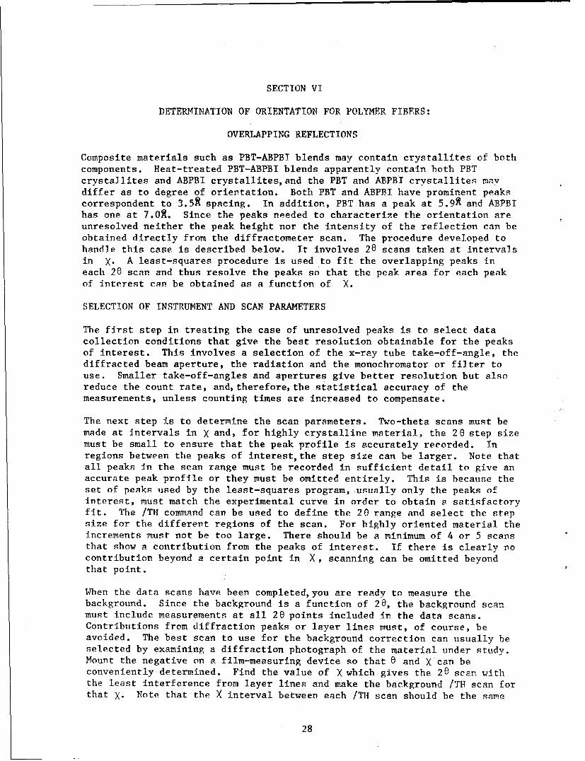
Composite materials such as PBT-ABPBT blends may contain crystallites of bothcomponents. Heat-treated PBT-ABPBI blends apparently contain both PBTcrystallites and ABPBI crystallites, and the PBT and ABPBi crystallites maydiffer as to degree of orientation. Both PBT and ABPBI have prominent peakscorrespondent to 3.5A spacing. In addition, PBT has a peak at 5.99 and ABPBIhas one at 7.09. Since the peaks needed to characterize the orientation areunresolved neither the peak height nor the intensity of the reflection can beobtained directly from the diffractometer scan. The procedure developed tohandle this case is described below. It involves 20 scans taken at intervalsin X. A least-squares procedure is used to fit the overlapping peaks ineach 20 scan and thus resolve the peaks so that the peak area for each peakof interest can be obtained as a function of X.

SELECTION OF INSTRUMENT AND SCAN PARAMETERS

The first step in treating the case of unresolved peaks is to select datacollection conditions that give the best resolution obtainable for the peaksof interest. This involves a selection of the x-ray tube take-off-angle, thediffracted beam aperture, the radiation and the monochromator or filter touse. Smaller take-off-angles and apertures give better resolution but alsoreduce the count rate, and, therefore, the statistical accuracy of themeasurements, unless counting times are increased to compensate.

The next step is to determine the scan parameters. Two-theta scans must bemade at intervals in X and, for highly crystalline material, the 20 step sizemust be small to ensure that the peak profile is accurately recorded. Inregions between the peaks of interest,the step size can be larger. Note thatall peaks in the scan range must be recorded in sufficient detail to give anaccurate peak profile or they must be omitted entirely. This is because theset of peaks used by the least-squares program, usually only the peaks ofinterest, must match the experimental curve in order to obtain a satisfactoryfit. The /TH command can be used to define the 20 range and select the stepsize for the different regions of the scan. For highly oriented material theincrements must not be too large. There should be a minimum of 4 or 5 scansthat show a contribution from the peaks of interest. If there is clearly nocontribution beyond a certain point in X, scanning can be omitted beyondthat point.

Wben the data scans have been completed, you are ready to measure thebackground. Since the background is a function of 20, the background scanmust include measurements at all 20 points included in the data scans.Contributions from diffraction peaks or layer lines must, of course, beavoided. The best scan to use for the background correction can usually beselected by examining a diffraction photograph of the material tinder study.Mount the negative on a film-measuring device so that 0 and X can beconveniently determined. Find the value of X which gives the 20 scan withthe least interference from layer lines and make the background /TI scan forthat X. Note that the X interval between each /TH scan should be the same

28

and each /TH scan must have measurements for the same set of 20 values.

DATA PROCESSING

When the data have been measured and written on the magnetic tape, translatedand entered into the off-site computer, you are ready to process it for inputto the curve fitting program. This program subtracts the background scanfrom the other scans point-by-point, makes the LP correction, and writes afile in a format corresponding to the input format required by the Andersonpeak fitting program (Anderson 1985). The preprocessing program has beenaffectionately named GALEN by one of us. Although the name is not verydescriptive, it is better than his usual porcine choices.

In the present example, fibers of the heat-treated PBT-ABPBI blend werescanned at values of 0', 4.50, 9.00, 13.50, 18.00, 22.50, 27.00, and 31.50.Inspection of the diffraction pattern of a similar fiber showed that onefeature on the 3.15' scan was due to the first layer line. The intensityvalues for that region were replaced by inserting a straight-lineinterpolation in place of the original intensities. The data file was thenrun through the preprocessing program.

Two theta scans for the lower X values show three peaks. Two at about 10degrees 20 (Cu Kadata) are barely resolved and a third at about 25 degrees 20appears to be resolved but is actually the sum of two peaks, one from eachcomponent of the blend. Samples of heat-treated PBT and heat-treated ABPBIphotographed separately show that the 25-degree peak is present in both.Preliminary attempts to fit the heat-treated blend with three peaks resultedin a poor fit in the region between the doublet and the main peak. It wasfound that a good fit could be obtained by assuming that the 25-degree peakwas the sum of two peaks with different width parameters.

Apparently one component of the blend has fairly sharp peaks at 10 degreesand 25 degrees and the other component has broader peaks at 11 degrees and 25degrees. Peak parameters are best defined on the scans atX = 00; thereforethe peak positions obtained on those scans should be used for fitting theother scans. The peak areas obtained at each X value can be used in theusual formula to calculate the orientation factor for each component. Thesame orientation factor should be obtained for each of the two peaks arisingfrom the same component. If interference from another layer line is present,the peak parameters will be inaccurate and that scan cannot be used. It mustthen be replaced by an estimated peak area, otherwise the orientation factorwill be incorrect. A better solution to the layer line problem would be tosubtract the intensity due to the interfering layer line before running thepreprocessing program. When this is done the peak parameters obtained by thefitting program should be accurate. If any peak height, area or width isnegative, you have a problem.

29

SECTION VII

DIFFRACTOMETER SCANS ALONG LAYER LINES FOR POLYMER MATERIALS

Polymer fibers give diffraction patterns which show cylindrical synmetry withthe diffraction maxima distributed in a series of layer lines. In highlyordered specimens,the layer lines are made up of individual reflections orgroups of reflections.

It is convenient to visualize the fiber pattern as it would appear ifrecorded on a precession film. If the fiber is vertical, the layer lines onthe film will be horizontal and a raster scan of the film will have one scandirection along the layer lines. The intensity variation along the layerlines will be gradual for materials of moderate order but will show sharpchanges for highly ordered materials.

The c* axis is, by convention, assigned to the layer line repeat which isparallel to the fiber axis, and the layer lines are then designated by the kindex. Because of the cylindrical symmetry of the pattern, either h or k corbe used to designate points along each of the layer lines.

The automated diffractometer can be used to measure the intensity along thelayer lines. This is conveniently done by using the single crystal routinesof the diffractometer control software. The method, as coded, requires anorientation matrix and cell. constants for a unit cell with c* parallel to the' axis of the diffractometer. Thus any fiber bundle that can be mountpd onthe diffractometer with the fiber axis parallel to the ý axis is suitable fora layer line scan. The only angles varied during the scan are 20 and •,sothe sample mount is not required to allow ý rotation except for opticalcentering and alignment.

The first step in preparing for a layer line scan is to center the fiber andensure that the fiber is exactly parallel to 4. If the specimen has sharpreflections on the meridian,one of these may be used. The goniometer headarcs must be adjusted so that the reflection is centered in the detectoraperture at X=90° and W=O°.

A convenient procedure for setting the fiber axis parallel to the axis of thediffractometer follows:

1. Use the diffractometer telescope to center the sample in the x-ray beamand align it as nearly as possible with the ý axis.

2. With X =90', rotate the sample so that one goniometer arc is vertical (inthe plane of the X circle).

3. Determine the profile of the strongest sharpest meridional reflectionpresent by making counts at appropriate intervals of X. For broad peaks,you may use X steps of 5°; for sharp peaks, smaller steps will berequired. The scan should extend at least 2/3 of the way down each sideof the peak.

4. Adjust the vertical. goniometer arc so the peak will be centered at

X =900.

30

5. Rotate the goniometer head and repeat steps 1. through 4 with the otherarc in the vertical position. Adjust it as required.

Note: The /PO command (see DIFF manual for details) can be used toobtain the X scans or you can drive X and use /PT and /ST tomeasure each point individually.

The procedure is similar if you have no suitable meridional reflection andmust use an equatorial reflection. For an equatorial reflection X must beset to zero.

The fiber repeat spacing must be accurately known. To find it, locate a

strong meridional reflection and scan it with the /TH command after setting

up a peak fit request with the /FT command. Use the layer line number andthe d spacing calculated by the peak fit procedure to find the c axis repeat.You are now ready to set up the cell constants and the orientation matrix.

Enter the cell constants with the /RP command. If the unit cell for thematerial being studied is not known, use a = b = c and U = ý = C = 900 (youhave determined c). The orientation is specified by two orientationreflections. The first must be an hO0 reflection with 6), X, and ý set tozero, the second an OkO reflection with 03 and X at zero and P= 900.Calculate the orientation matrix with /CM and display it with /CA aftersetting the wavelength with /WV.

You are now ready to choose the scan parameters for the layer line scan. Ifyou have a precession film, you can use it as a guide. The layer lines areeasily counted to obtain -the scan limits which are denoted as the k index.The length of scan along each layer line is specified by a start and stopvalue for k. If you have used a = b = c for the cell constants, each unit ofk will span a length equal to the distance between each layer line on aprecession film.

Enter the preset time with /PT to be used for each point measured and thenenter the scan limits with /LL. The interval for k will be governed by thedegree of order in your sample. Values of 0.2 and 0.5 are often used. Notethat since b is arbitrary, the k scan parameters are not related to the realk index. The interval for t is usually 0.5 so that a background scan isincluded between each layer line.

Table 9 lists data for a first layer line scan on ABPBT fibers, which areplotted in figure 6.

31

TABLE 9. EYAMPLE OF FACS-I INPUT-OUTPUT FOR A LAYER LINE SCAN FOR AHEAT-TREATED ABPBT SAMPLE.

/WV

1.5418

/PT7

/RP

12.19 12.12 12.19 0 0 0 5 0 0 0 0 0 0 5 0 0 0 90

1Cll

/CA

12.19001 12.18999 12.19000 0.00000 0.00000 0.00000

-0.0820344 0.0000000 0.0000000

0.0000000 -0.0820345 0.0000000

0.0000000 0.0000000 -0.0820345

1.541799 1811.39

/FT0/LL

0 1 1 -5 .1 5

0.00 -5.00 0.00

0.69 0.59 0.56 0.63 0.65 0.67 0.75 1.09 1.47 2.36 2.93

3.65 6.90 17.78 28.66 28.25 21.20 12.47 5.89 3.16 2.38 1.78

1.66 1.61 1.48 1.55 1.55 2.36 4.11 15.47 25.45 6.15 2.26

1.39 1.20 1.19 1.14 1.15 1.24 1.29 1.33 1.35 1.55 2.04

2.49 3.27 6.50 4.99 0.29 0.22 0.22 0.26 0.33 5.01 6.65

3.06 2.27 1.74 1.51 1.30 1.21 1.00 1.13 1.25 1.18 1.35

1.32 1.50 2.13 6.28 26.13 15.89 3.98 2.17 1.74 1.65 1.59

1.45 1.73 1.81 2.29 3.27 6.10 11.95 20.73 28.21 28.90 17.15

7.23 3.62 3.09 2.58 1.73 1.09 0.73 0.77 0.59 0.65 0.56

32

C3

0

C3

0

(I)

o(aC')

44,

0

ro

2L

33w

SECTION VIII

POLE FIGURE DATA COLLECTION AND ANALYSIS

The Picker FACS-I automated diffractometer is ideally suited to collecttwo-dimensional diffraction data on polycrystalline specimens. These datacan be used to determine and display the orientation of the crystallites inthe sample in the form of a pole figure diagram. The two diffractiongeometries in common use, reflection and transmission, are shown in figure 7(Desper, 1969).

20A, x Axis

(•-0)

Beam

Axis

X-Ray DFixed)

Diffracted 4

BeamBe

(a) (b)

Figure 7. Pole Figure Geometry, (a) Reflection and (b) Transmission Methods

One cannot measure a complete pole figure in either the transmission or the

reflection mode selected by MTO=I or MTHD=0 in the FACS-I P0 command. In

the transmission mode all values of X are available on the diffractometer but 0

is restricted to angles between 0 and 450. This range allows about 2/3 of

the pole figure to be measured. In the reflection mode all values of c• are

available but there may be mechanical restrictions on values of X near 00.

At low 26 angles the x-ray beam becomes almost parallel to the sample even at

moderate values of . The FACS-I control program includes commands for pole

figure data collection which are an extension of those described by Desper

(1969).

When starting a pole figure run, be sure to write all instrument parameters on

the magnetic tape after initiating it with /TS. Example input is given in

table 10 below.

S34

TABLE 10. EXAMPLE OF TAPE HEADING.

/TS

/TY

Data for PBT-27554-33-4(2)This sample is a bundle of fibers approximately 0.6 mm In diameter. It ismounted vertical in the diffractometer. The scan in 2 Theta will thereforebe a scan of the equatorial reflections.

TOA is 3.2DEG (Nominal), Actual TOA is 3.0 DEG.SVA is wide open.HOG monochromator XTAL is in place and Beam uniformity is satisfactory (justchecked).Mono angle is 12.16 and PSI is 6.05.Incident and diffracted beam collimators are 1.0 mm.No filters are used.KV 50 MA 12.Analyzer upper 7.0, Lower 4.0, 100% HT centered at 5.20.Gain at 10, fine focus molybdenum tube.

Smaller SVA and smaller TOA do not seem to improve the resolution.

35

The transmission mode is most useful for polymer samples. Job parameters fora transmission mode example are shown in table 11.

TABLE 11. TRANSMISSION MODE POLE FIGURE INPUT AND OUTPUT.

/PT6/FP5 3.2/P0MTHD=iTH=7.35 TH=0OM-0 DLSN=.1 NPTS-8 CR=0 CLCH=2.5 NPTS=37TH= 7.35 OM= 0.00 CH= 0.00 PH= 0.00

OM- 0.0010.27 11.95 12.62 11.67 10.32 7.32 5.40 4.40 2.00 1.050.65 0.60 0.27 0.55 0.05 0.35 -0.18 0.15 -0.25 0.10

-0.10 -0.05 -0.07 0.17 0.25 0.13 0.38 0.40 0.15 0.200.00 0.05 -0.10 -0.05 -0.40 -0.28 -0.28

OM=5.7410.47 11.42 11.57 11.12 9.00 7.05 4.92 2.55 1.55 1.050.63 0.55 0.55 0.43 0.32 0.20 -0.05 0.00 -0.17 -0.250.03 -0.10 0.25 0.22 0.30 0.35 0.38 0.42 0.17 0.15

-0.05 0.15 0.07 -0.15 -0.30 -0.25 -0.40OM= 11.5410.70 11.85 12.02 10.97 8.77 6.57 4.40 2.83 1.47 0.770.45 0.32 0.13 0.28 0.02 0.03 0.03 0.03 0.00 -0.130.07 -0.07 0.07 0.20 0.17 0.43 0.43 0.25 0.38 0.35

OM= 17.4611.12 12.25 11.75 10.70 9.07 6.70 4.35 2.70 1.58 0.820.53 0.57 0.15 0.28 0.20 0.30 -0.07 0.10 0.13 0.07

-0.20 -0.20 -0.03 0.17 -0.13 0.18 0.28 0.50 0.60 0.450.35 0.30 0.30 0.30 0.05 0.13 0.18

OM= 23.5811.00 12.12 12.20 11.32 9.15 6.65 4.55 2.77 1.75 0.850.77 0.48 0.50 0.25 0.53 0.20 0.40 -0.05 0.07 -0.15

-0.05 -0.43 -0.10 -0.03 0.05 0.18 0.15 0.45 0.50 0.530.63 0.50 0.70 0.53 0.45 0.40 0.38

OM= 30.0012.20 12.72 12.67 11.42 9.47 7.65 5.15 3.40 1.95 1.100.50 1.30 0.60 0.73 0.63 0.73 0.50 0.25 0.32 0.05

-0.20 -0.13 -0.10 -0.27 -0.10 -0.10 -0.05 0.17 0.10 0.220.35 0.63 0.70 0.57 0.75 0.75 0.75

OM= 36.8715.65 17.45 17.45 17.10 14.98 12.35 10.35 7.65 5.85 3.772.42 1.67 1.28 0.77 0.85 0.47 0.68 0.63 0.35 0.200.07 0.15 -0.25 -0.23 -0.13 -0.27 -0.10 -0.13 -0.15 0.i00.15 0.28 0.30 0.57 0.60 0.57 0.83

OM= 44.4317.92 19.80 19.72 19.00 17.58 15.45 12.97 10.23 7.80 5.803.95 2.72 1.93 1.47 1.18 0.63 0.77 0.57 0.50 0.330.18 0.80 0.75 1.25 1.80 3.03 3.52 4.55 5.40 6.256.75 7.85 8.18 8.53 8.72 9.55 9.53

36

The Intervals in this examp]e for ANGLE 1 and ANGLE 2 (LOand X) aresatisfactory for most polymer work. Smaller increments would be advisable ifthe sample were highly crystalline. Counting time should be chosen so thatvalues near the peak will have at least 2000 counts per measurement. If timepermits, more counts will give an improved pole figure in most cases. If abackground correction is made, the total time spent counting the backgroundshould be about equal to that spent measuring the peak.

The scan range (for the integral mode) or the width of the peak (for the /FBmode) should be carefully chosen. A 20 scan using the /TH command will givethe peak profile and facilitate the choice of optimal end points for thescan. Include all of the peak if possible, but stay clear of adjacent peaks.An example of /TH use is given in table 12.

TABLE 12. TWO-THETA SCAN FOR A BUNDLE OF PBT FIBERS. (PART OF OUTPUT ISOMITTED).

/TY

START 2 THETA EQUATORIAL SCAN AT 5 PM AUG. 4, 1980

/THTH=29. DLTH=.l TH=29. DLTH=04.66 4.71 4.65 4.52 4.61 4.65 4.72 4.91 4.88 4.935.02 4.96 4.98 4.83 5.05 5.03 5.11 5.28 5.28 5.285.36 5.39 5.60 5.82 5.72 5.86 5.95 6.19 6.26 6.376.36 6.75 6.85 7.01 7.15 7.34 7.61 7.92 8.13 8.348.70 8.75 8.90 9.36 9.45 9.80 9.82 10.06 10.28 10.53

10.66 10.78 11.04 11.24 11.47 11.25 11.62 11.60 11.59 11.5011.65 11.35 11.45 11.28 11.34 11.09 10.86 10.43 10.55 10.2310.01 9.85 9.55 9.53 9.36 9.04 8.89 8.77 8.67 8.508.18 8.24 8.24 8.05 7.88 7.80 7.79 7.60 7.73 7.627.48 7.31 7.42 7.29 7.24 7.14 7.19 6.98 6.98 6.987.08 6.84 6.82 6.76 6.91 6.79 6.76 6.69 6.72 6.436.50 6.58 6.50 6.41 6.57 6.39 6.48 6.57 6.52 6.706.52 6.65 6.72 6.75 6.87 7.01 6.89 7.02 7.27 7.337.44 7.50 7.78 8.04 8.34 8.38 8.85 9.28 9.64 10.23

10.73 11.48 12.17 13.02 14.04 15.25 16.75 18.39 19.91 21.9624.20 26.55 29.17 32.11 35.44 38.67 42.67 46.86 50.94 56.6362.26 67.38 73.57 80.16 85..86 91.93 96.62 102.00 105.38 107.99

110.02 110.55 110.68 109.62 107.95 105.15 100.88 96.01 92.36• 86.7081.47 75.69 70.47 65.12 61.01 56.41 53.04 50.27 47.34 45.4943.57 42.39 40.98 39.88 38.93 38.26 37.90 37.22 36.64 36.8436.67 36.53 37.01 37.28 37.72 38.36 39.07 39.68 41.18 42.5343.71 45.26 46.69 48.65 49.76 50.56 51.61 51.82 51.85 51.80

37

A satisfactory run could have been obtained for this material with a largerstep size. A shorter counting time (40s rather than 100s) would also havebeen satisfactory. The scan was run from -20 to +20 which is desirable butnot necessary.

Parameters for UNIAXIAL scans for this PBT fiber bundle are shown in tables13 and 14.

TABLE 13. UNIAXIAL SCANS FOR PBT. NO BACKGROUND NECESSARY.

/PT6/FM/TYREADY FOR 7.15 POLY FIGURE WITHOUT BKG MEAS BUT WITH MONOCHROMATOR/POMTHD=1TH=7.15 TH=0OM=0 DLSN=0 NPTS=1 CH=O DLCH=2.5 NPTS=37TH= 7.15 OM= 0.00 CH= 0.00 PH= 0.00OM= 0.0057.25 48.75 37.80 28.85 21.65 16.77 13.70 12.15 11.27 10.6010.20 9.70 9.20 8.52 8.00 7,45 7.25 6.72 6.67 6.886.85 6.88 7.05 6.90 6.92 6.63 6.55 6.38 6.02 5.775.42 5.60 5.25 5.07 5.07 5.10 5.10

TABLE 14. UNIAXIAL SCAN FOR PBT WITH BACKGROUNDS MEASURED FOR 20 S EACH, 1.30ABOVE AND BELOW THE PEAK POSITION.

0

1.3 above and below the peak position.

/TYNOW DO IT AGAIN WITH BACKGROUND SUBTRACTED/FB5 2.6/POMTHD=-1TH=7.15 TH=OOM=0 DLSN=0 NPTS=1 CH=0 DLCH=2.5 NPTS=37TH= 7.15 ON=- 0.00 CH= 0.00 PH= 0.00OM= 0.0022.70 18.28 13.17 8.15 4.73 2.83 1.50 1.25 0.55 1.250.23 0.85 0.33 0.70 -0.38 -0.02 -0.33 -0.25 0.05 -0.170.20 0.67 0.47 1.12 1.38 1.27 1.10 1.05 0.77 0.750.47 0.63 0.55 0.40 0.40 0.10 0.07

38

THE MONOCHROMATOR AND BACKGROUND CORRECTIONS

Comparison of several PBT pole figures indicates that a background correctionmust be made to get an accurate pole figure. Best results will be obtainedwith a continuous scan (IM mode) but /FB will give a satisfactory result in ashorter time. The nonochromator gives a cleaner pole figure than one getswith filtered radiation, but its use is not mandatory.

COMBINING TRANSMISSION AND REFLECTION POLE FIGURES WITH POLEDAT

The POLEDAT PROGRAM (Desper, 1978) will combine transmission and reflectionpole figures to give a complete pole figure. There are two requirements.One must make the volume correction (and absorption correction if needed),and it is imperative that the angle ranges and increments be compatible forboth measurements. Use the same increment for ANGLE I and ANGLE 2 for bothtransmission and reflection.

For transmission (MTHD=I) omega must start at zero. It may increase ordecrease. Chi is not restricted but if you want only one quadrant, start atzero and go to 900.

For reflection (MTHD=O), phi must start at zero and increase. Chi usuallystarts at 40' and increases to 900. This gives sufficient overlap with thetransmission data to complete the pole figure.

The MERGE feature of POLEDAT has not been tested at Wright-Patterson AirForce Base.

USING POLEDAT

The CONLEV card should be used if CALCOMP contour plots are to be drawn.

The ABTH card must be used to get the volume correction. The input parameteris 0 if no absorption correction is desired. AbsorptionV, can beconveniently measured with the monochromator in place by determining I (nosample) and I with the sample in the direct beam (be sure to restrict ?hebeam to protect the counter). Remember I/I =e-•t.

0

Set KOORD=1 for samples with the machine direction mounted parallel to thePHI axis and the Sheet normal parallel to the Chi axis. This is the usualarrangement.

THE ORIENTATION FACTOR

The orientation factor for a pole figure analysis is calculated by POLEDAT,but only if data for a complete pole figure is available. One can get theorientation factor for transmission data if the program is given the extradata. This can be done by editing the data file with the PRIME 850 editor.Change the angle limits and supply the extra data points with zero or verysmall values. (It goes without saying that the pole density in the region offabricated data had better be zero or you will be in trouble). POLEDAT thusfooled will give the orientation factors.

39

For the transmission case with KOORD=l the average squared direction cosine5'for the x, y, and z axes will be:

1. If the poles are at W=0 and X=90

(Cosx2 ) =0 pole density

(Cs ) =0

(Cos z2) =1

2. If the poles are at W =0 and X=0

(cs2(Cosx =0y

(cos 2

(o 2 =--pole density

3. If the poles are at w=90 and X=O to 90

(Cosy2 ) =2

(cos 2 =0

( pole density_--r

40

REFERENCES

Anderson, David P. (1985), "X-ray Analysis Software Operation and TheoryInvolved in Program "DIFF", AFWAL-TR (In Preparation).

Desper, C. Richard (1969), "A Computer-Controlled X-ray Diffractometer forTexture Studies of Polycrystalline Materials," Advances in X-ray Analysis 12,404-417.

Desper, C. Richard (1978), "Computer Programs for Reduction of X-rayDiffraction Data for Oriented Polycrystalline Specimens," Report ANNRCTR-72-34, Army Materials and Mechanics Research Center, Watertown, MA.

Lenhert, P. Galen (1974), "Vanderbilt Disk-Oriented Diffractometer System, AUser'sManual," Physics Department, Vanderbilt University.

Lenhert, P. Galen (1978), "Diffractometer Alignment, 4-Circle Instruments,"ACA Tutorial - March 19, 1978, University of Oklahoma.

Lenhert, P. Galen (1980), "A Simple Method for Testing X-ray BeamUniformity," Journal of Applied Crystallography, 13, 199.

Stein, R. S. (1958), Journal of Polymer Science, 31, 327.

4U.S.Government Printing Office: 1987 - 748-061/6077341