AFTAC-TR-09-006 AFTAC · Report AFTAC-TR-09-006 has been ... In this paper we present a routine...
26
AFTAC Air Force Technical Applications Center Directorate of Nuclear Treaty Monitoring Automated Source Depth Estimation Using Array Processing Techniques W.N. Junek, J. Roman-Nieves, R.C. Kemerait, M.T. Woods, and J.P. Creasey 14 October 2009 Approved for public release; Distribution is unlimited. AFTAC-TR-09-006
Transcript of AFTAC-TR-09-006 AFTAC · Report AFTAC-TR-09-006 has been ... In this paper we present a routine...

AFTAC Air Force Technical Applications Center
Directorate of Nuclear Treaty Monitoring
Automated Source Depth Estimation Using Array Processing Techniques
W.N. Junek, J. Roman-Nieves, R.C. Kemerait, M.T. Woods, and J.P. Creasey
14 October 2009
Approved for public release;
Distribution is unlimited.
AFTAC-TR-09-006

Report AFTAC-TR-09-006 has been reviewed and is approved for publication.
LISA ANN H. ONAGA, C onel, USAF Commander
Addressees: Please notify AFTAC/TT, 1030 South Highway AlA, Patrick Air Force Base, Florida 32925-3002, if there is a change in your mailing address (including an individual no longer employed by your organization) or if your organization no longer wishes to be included in the distribution of future reports of this nature.
ii

iii
REPORT DOCUMENTATION PAGE Form Approved
OMB No. 0704-0188 Public reporting burden for this collection of information is estimated to average 1 hour per response, including the time for reviewing instructions, searching existing data sources, gathering and maintaining the data needed, and completing and reviewing this collection of information. Send comments regarding this burden estimate or any other aspect of this collection of information, including suggestions for reducing this burden to Department of Defense, Washington Headquarters Services, Directorate for Information Operations and Reports (0704-0188), 1215 Jefferson Davis Highway, Suite 1204, Arlington, VA 22202-4302. Respondents should be aware that notwithstanding any other provision of law, no person shall be subject to any penalty for failing to comply with a collection of information if it does not display a currently valid OMB control number. PLEASE DO NOT RETURN YOUR FORM TO THE ABOVE ADDRESS.
1. REPORT DATE (DD-MM-YYYY)
14 October 2009 2. REPORT TYPE
Technical 3. DATES COVERED (From - To)
4. TITLE AND SUBTITLE
5a. CONTRACT NUMBER
Automated Source Depth Estimation Using Array Processing Techniques
5b. GRANT NUMBER
5c. PROGRAM ELEMENT NUMBER
6. AUTHOR(S)
5d. PROJECT NUMBER
W.N. Junek, J. Roman-Nieves, R.C. Kemerait, M.T. Woods, and J.P. Creasey
5e. TASK NUMBER
5f. WORK UNIT NUMBER 7. PERFORMING ORGANIZATION NAME(S) AND ADDRESS(ES)
AND ADDRESS(ES)
8. PERFORMING ORGANIZATION REPORT NUMBER
Air Force Technical Applications Center
AFTAC/TT
1030 S. Hwy A1A
Patrick AFB FL 32925-3002
AFTAC-TR-09-006
9. SPONSORING / MONITORING AGENCY NAME(S) AND ADDRESS(ES) 10. SPONSOR/MONITOR’S ACRONYM(S)
11. SPONSOR/MONITOR’S REPORT
NUMBER(S)
12. DISTRIBUTION / AVAILABILITY STATEMENT
A – Approved for public release; distribution is unlimited.
13. SUPPLEMENTARY NOTES
14. ABSTRACT
In this paper we present a routine that exploits the power of seismic arrays and cepstral techniques to estimate the depth of an
event directly from the observed seismograms. A discussion of the pertinent geophysical assumptions, cepstral processing
algorithm, stable peak identification via “cepstrograms,” false alarm reduction methodology, and our array-based depth
estimation routine is presented. An analysis of several shallow events is performed and compared to results produced by a
standard location algorithm, waveform forward modeling, and previously published solutions.
15. SUBJECT TERMS
Cepstrum Depth Estimation Array Processing Signal Processing Seismology
17. LIMITATION OF ABSTRACT
18. NUMBER OF PAGES
19a. NAME OF RESPONSIBLE PERSON
William N. Junek a. REPORT
UNCLAS
b. ABSTRACT
UNCLAS
c. THIS PAGE
UNCLAS
SAR
23
19b. TELEPHONE NUMBER (include area
code)
321-494-8202 Standard Form 298 (Rev. 8-98)
Prescribed by ANSI Std. Z39.18

iv
(This page intentionally left blank)

Automated Source Depth Estimation
Using Array Processing Techniques
v
Abstract
In this paper we present a routine that exploits the power of seismic arrays and cepstral
techniques to estimate the depth of an event directly from the observed seismograms. A
discussion of the pertinent geophysical assumptions, cepstral processing algorithm, stable peak
identification via “cepstrograms,” false alarm reduction methodology, and our array-based depth
estimation routine is presented. An analysis of several shallow events is performed and
compared to results produced by a standard location algorithm, waveform forward modeling, and
previously published solutions.

Automated Source Depth Estimation
Using Array Processing Techniques
vi
Acknowledgments
The authors would like to thank the Romanian Geophysics institute, Kazakhstan National
Nuclear Center Institute of Geophysical Research, NORSAR, and the Republic of Turkey
Kandilli Observatory and Earthquake Research Institute for allowing us to use data from their
stations. We would especially like to thank Dr. G. Randall, Dr. D. Russell, Dr. G. Wagner,
Dr. G. Ichinose, and Mr. J. Dwyer for their assistance and advice in performing this research.
The figures shown in this report were generated using the Generic Mapping Tool (GMT). In
addition, we are grateful to Ms. S. Fisher for editing and reviewing this report.

Automated Source Depth Estimation
Using Array Processing Techniques
vii
Contents
Abstract ...........................................................................................................................................v
Acknowledgments ......................................................................................................................... vi
List of Figures ............................................................................................................................. viii
List of Tables .............................................................................................................................. viii
1.0 Introduction .............................................................................................................................1
2.0 Theory .....................................................................................................................................2
2.1 Depth Estimation .............................................................................................................3
2.2 Signal Processing Algorithm ...........................................................................................4
2.2.1 Cepstral Processing ...............................................................................................5
2.2.2 False Alarm Reduction ..........................................................................................5
2.2.3 Depth Computation ...............................................................................................7
3.0 Discussion ...............................................................................................................................7
4.0 Summary ...............................................................................................................................10
References .....................................................................................................................................12
Distribution ...................................................................................................................................14

Automated Source Depth Estimation
Using Array Processing Techniques
viii
List of Figures
Figure 1a Propagation paths for primary and associated depth phases .........................................3
Figure 1b Ideal ray path geometry for a seismic point source ......................................................3
Figure 2 Signal processing algorithm ..........................................................................................4
Figure 3 Conceptual cepstrograms ..............................................................................................6
Figure 4a Event #3: 2003 Bhuj aftershock location, focal mechanism, and network
configuration .................................................................................................................8
Figure 4b Seismograms observed by each station and separated as a function of distance ..........8
Figure 5a Cepstrograms for BURAR, BRTR, FINES, and KSRS ................................................9
Figure 5b Frequency wavenumber plots .......................................................................................9
Figure 5c Network-based depth estimate ......................................................................................9
List of Tables
Table 1 Comparison of Results ...................................................................................................10

Automated Source Depth Estimation
Using Array Processing Techniques
1
Automated Source Depth Estimation Using Array Processing Techniques
1.0 Introduction
Source depth estimation is a key process in the discrimination of earthquakes and explosions.
The lack of observable depth phases does not necessarily mean the event occurred at or near the
surface. Shallow events can have closely spaced depth phases that are indistinguishable even by
seasoned human analysts. Moreover, the onset of smaller events observed at regional distances
is often complicated by the arrival of multiple phases in rapid succession, which makes the
identification of depth phases even more problematic. Source parameters for such events can be
derived using moment tensor inversion or forward modeling techniques, which are difficult to
apply to events less than mb 5.5 and shallower than 15 km, and depend on the availability and
accuracy of geophysical models. These limitations are not practical for real-time discrimination
of earthquakes and explosions.
If depth phases with sufficient signal-to-noise ratio (SNR) reside in an observation, they will
produce a spectral scalloping pattern with a period equal to the time delay between signals. This
spectral phenomenon can be detected using cepstral processing, which has been used in a
number of studies over the last 45 years with limited success [Bogart et al., 1963; Ulrych, 1971;
Kemerait and Childers, 1972; Ulrych et al., 1972; Tribolet, 1978; Kemerait and Sutton, 1982;
Marenco and Madisetti, 1997; Shumway et al., 1998; Bonner et al., 2002; and Reiter, 2005].
These studies, however, did not exploit the power of seismic arrays to determine the ray
parameter of the arriving phase. The ray parameter, an assumed wave speed, and simple vector
decomposition can be used to determine the vertical phase velocity and wavefront angle of
incidence. If reciprocity between the source and receiver holds, the angle of incidence and take-
off angle are the same and can be combined with the depth phase delay time to calculate a source
depth directly from the observed seismograms. Unlike moment tensor inversion or waveform
forward modeling, this methodology neither requires detailed geophysical models nor is
restricted to large events or a minimum depth.
Our routine employs a multi-stage detection scheme that reduces the high false alarm rate
inherent to cepstral analysis. First, a site-specific, adaptive, cepstral amplitude or gamnitude

Automated Source Depth Estimation
Using Array Processing Techniques
2
threshold, recalling the terminology coined by Bogart et al., 1963, is derived using pre-signal
noise to identify statistically significant peaks. Knowing that cepstra are highly unstable and
change significantly with minor changes to processing parameters, we developed an iterative
technique to search for stable detections over a series of increasing time windows. The resulting
“cepstrograms” accentuate stable features in the cepstral domain to assist the algorithm in
selecting only signal-induced peaks. Finally, a binary stacking module checks for consistent
detections across the observing network.
2.0 Theory
Figure 1a shows the ray path geometry between a shallow source and receiver. Notice that
upward traveling rays reflect off the free surface, travel along a path similar to the primary phase,
and arrive at the receiver with the same angle of incidence and apparent velocity. This idealized
illustration depicts the geophysical assumptions our algorithm relies on, which are as follows:
Source Mechanism: Cepstral analysis relies on the assumption that the source
mechanism can be modeled as a point source. Large magnitude earthquakes often have
time varying rupture processes that violate this assumption. As a result, we limit
ourselves to analyzing events with bodywave magnitudes less than 6.0.
Phase Speed: Since we are interested in discriminating between earthquakes and
explosions, we assume a shallow source depth (d < 20 km). This means that the speed of
the incident P-wave is approximately 5.8 km/sec for continental crust events [Kennett,
1991].
Angle of Arrival: If reciprocity holds, the incidence angle of the primary arrival is equal
to the take-off angle at the source. This assumption allows for the derivation of the take-
off angle using horizontal apparent velocity measurements and the previously assumed
phase speed.
Stephanie.Fisher
Line

Automated Source Depth Estimation
Using Array Processing Techniques
3
(a) (b)
Figure 1. (a) Propagation paths for primary arrival and associated depth phases traveling through a flat,
discretized earth. (b) Ideal ray path geometry for a seismic point source.
2.1 Depth Estimation
The ray transmission and reflection geometry generated by a seismic point source is shown in Figure
lb. The illustration shows depth, d (km), is a function of the delay time between the primary arrival and
its associated depth-phase, (sec), the ray take-off angle, (deg), and the P wave speed, α (km/s)
d = ( * ) cos2
1
(1)
The value of is supplied via cepstral processing (section 2.2.1) and the ray take-off angle is computed
using the phase velocity's horizontal and vertical components. The horizontal phase velocity or apparent
velocity, c (s/km), of a planar wavefront traveling across a seismic array is often measured using
frequency-wavenumber analysis [Kvaerna, 1989]. The apparent velocity measurement of the incident
wavefront, and an assumed speed of the P-wave, allows us to calculate the ray's vertical velocity
component, (s/km), and take-off angle using
(2)
c
1tan
(3)
respectively.
Stephanie.Fisher
Stamp

Automated Source Depth Estimation
Using Array Processing Techniques
4
Since the take-off angle and apparent velocity vary as a function of distance, due to varying ray path
geometries, they are calculated for each station in the network. Site-specific values for , c, and are
computed and substituted into (1) [Junek et al., 2006; Junek et al., 2007]. This results in a suite of depth
hypothesis that already account for move-out between stations.
2.2 Signal Processing Algorithm
Our signal processing algorithm (Figure 2) consists of three main components. First, a cepstral
processing component (cyan) determines the time delays between direct P and the reflected phase. Next,
a depth estimation component (yellow) combines delay times with phase wavespeeds to compute a depth.
Finally, a false alarm reduction component (green) identifies statistically significant cepstra and
consistent depth estimates across the network.
Figure 2. Signal processing algorithm consists of a cepstral processing component (cyan), depth
estimation component (yellow), and a false alarm reduction component (green).

Automated Source Depth Estimation
Using Array Processing Techniques
5
2.2.1 Cepstral Processing
Our cepstral processing function combines the methodologies of [Kemerait, 1972; Shumway et al.,
1998; and Bonner et al., 2002]. Event observations and pre-signal noise segments from each element of
an array are passed into the algorithm and processed separately using the same parameters to ensure the
results are comparable. Mean signal and pre-signal noise cepstra are created from the individual results to
enhance common peaks.
2.2.2 False Alarm Reduction
The false alarm reduction routine consists of four primary components: gamnitude threshold
computation, detection processing, application of a cepstral stability requirement, and a network
consistency check. Each of these techniques is used to reduce the high false alarm rate inherent to
cepstral analysis.
A gamnitude threshold derived from site-specific, pre-signal noise cepstra is used to select candidate
peaks for the depth estimation algorithm. The threshold is defined as the 99th percentile of the gamnitude
distribution of the pre-signal noise cepstra for a sampling window equal to the time-domain sampling
window. This is repeated for each station in the network to derive real-time, site-specific gamnitude
thresholds that are based on the current noise conditions at each site. This prevents hourly, daily, or
seasonal noise fluctuations from increasing the false alarm rate.
Cepstral processing is performed for each station using a series of increasing sampling window
lengths to identify stable peaks. As the sampling window length grows and captures larger sections of the
depth phase, the intensity of the points in the “cepstrograms” grows, peaks, and fades as more noise is
acquired. A stability parameter, , is used to define the number of consecutive threshold crossing cepstra
that are required to declare candidate depth phase detections. The value of is typically set between 15%
and 25% of the total number of sampling windows. Results existing for less than this value are not
considered a candidate depth phase. Figure 3 shows conceptual cepstrograms for both pre-signal noise

Automated Source Depth Estimation
Using Array Processing Techniques
6
and the observed seismogram. This procedure is repeated for each set of array observations until a
collection of cepstrograms are generated.
Figure 3. Conceptual cepstrograms for pre-signal noise and observed seismograms, respectively, where
the Y-axis is delay time, X-axis is the sampling window length, random points in the top and
bottom panels are transient noise spikes, and lines are stable signals.
Detection processing is carried out on a station-by-station basis. All threshold crossing cepstra, for
each station, that meet the stability criteria are treated equally to avoid the possibility of a missed
detection. Each candidate depth phase delay time is then passed to the depth estimator (section 2.2.3).
Network consistency is checked by a binary stacking algorithm and takes place after depth extraction
to compensate for move-out between stations [Murphy et al., 1999; Bonner et al., 2002]. This
methodology allows one input per station for each depth cell, whose width is a user defined parameter, n
[Bonner et al., 2002; Murphy et al. 1999]. The largest peak in the stack identifies the measurement that is
the most consistent across the network and is declared the final result.

Automated Source Depth Estimation
Using Array Processing Techniques
7
2.2.3 Depth Computation
The depth estimation module requires time domain data for the primary arrival and the time delay of
each threshold crossing cepstra for each station being considered. Time domain data is used to compute c
of the incident wavefront, which is used to compute and . These parameters are substituted into
equation (1) to calculate a suite depth estimates for that seismogram. This is repeated for each array in
the network, where the resulting depth profiles are passed to the network consistency routine (section
2.2.2).
3.0 Discussion
Automated depth estimates for a series of events observed at regional and teleseismic distances were
generated and compared to those derived by a standard location routine, moment tensor inversion and
waveform forward modeling, and previously published results. Five randomly selected events are chosen
for our evaluation. Filter passbands that maximize the signal-to-noise ratio for each station/event pair
were selected and a standard set of processing parameters were used to prevent tuning biases in the
solutions.
Models for events 1, 2, 4, and 5 were computed using the Moment Tensor Inversion Toolkit
(MTINV) [Ichinose, 2006] and regional data acquired from IRIS or the Japanese Meteorological Agency
(JMA). Simple three-layer crustal models over a half space were used to model these events, where the
Western United States model was used for events 2 and 5, a model created by [Ichinose, 2008] was used for
event 4, and a modified version of a model-based one [Ichinose et al., 2005] was used for event 1. Event
3 was modeled using reflectivity software employing Kennett's technique of solving wave propagation
problems in laterally homogenous layers [Randall et al., no date]. A 186-layer Earth model consisting of a
two-layer crust, similar to one used by [Antolik and Drenger, 2003], and an upper and lower mantle
model based on PREM was used to compute the synthetics [Randall, 2006].
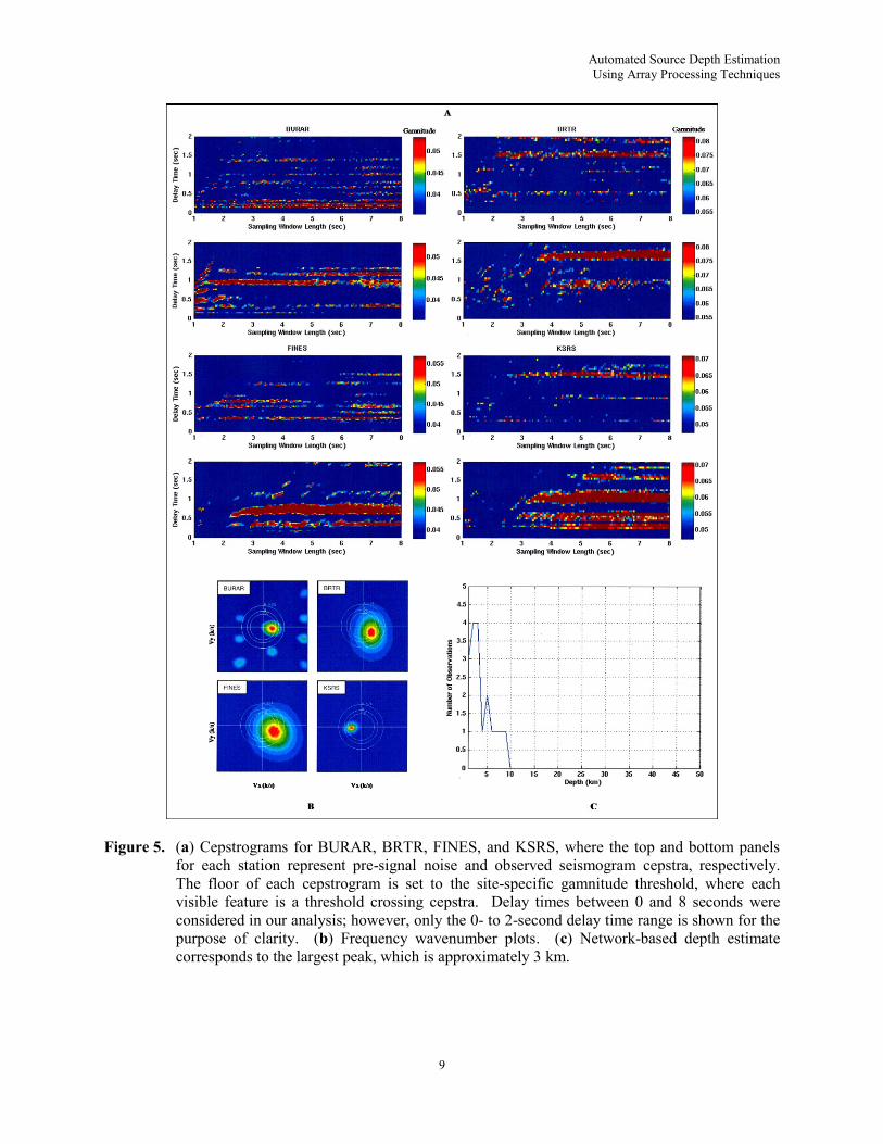
Observed waveforms, network configuration, and automated processing results for event 3 are shown
in Figures 4 and 5. Cepstra for each station were generated for a series of sampling window lengths

Automated Source Depth Estimation
Using Array Processing Techniques
8
between 0.0 sec and 8.0 sec in increasing increments of 0.05 sec. Resulting cepstrograms and frequency
wavenumber plots are shown in Figures 5a and b, respectively. Notice there are numerous features in
each cepstrogram. The before mentioned stability parameter screened out the transients and passed only
stable features to the depth computation module. The final depth estimate is shown in Figure 5c and is
approximately 3 km.
(a) (b)
Figure 4. (a) Event #3: 2003 Bhuj aftershock location, focal mechanism, and network configuration.
(b) Seismograms observed by each station and separated as a function of distance.
Stephanie.Fisher
Typewritten Text
BRTR
Stephanie.Fisher
Typewritten Text
BURAR
Stephanie.Fisher
Typewritten Text
FINES
Stephanie.Fisher
Typewritten Text
KSRS
Automated Source Depth Estimation
Using Array Processing Techniques
9
Figure 5. (a) Cepstrograms for BURAR, BRTR, FINES, and KSRS, where the top and bottom panels
for each station represent pre-signal noise and observed seismogram cepstra, respectively.
The floor of each cepstrogram is set to the site-specific gamnitude threshold, where each
visible feature is a threshold crossing cepstra. Delay times between 0 and 8 seconds were
considered in our analysis; however, only the 0- to 2-second delay time range is shown for the
purpose of clarity. (b) Frequency wavenumber plots. (c) Network-based depth estimate
corresponds to the largest peak, which is approximately 3 km.

Automated Source Depth Estimation
Using Array Processing Techniques
10
Table 1 shows a comparison of depth estimates for the analyzed events. Values listed in the “Array-
Based” column were produced by our routine, free-depth solutions were created using a location
algorithm based on [Jordan and Sverdrup, 1981], and published solutions were obtained from several
organizations, which are referenced in Table 1. Our results are in good agreement with the published and
free-depth solutions and correspond particularly well to the modeled results.
Table 1: Comparison of Results
Event Origin Time (GMT) Latitude (°) Longitude (°) mb
Depth (km)
Published Array-
Based Modeled
Free-
Depth
1* 05/06/2002, 08:12:14 38.4° 141.2° 5.1 40 35 35 45
2**
03/12/2005, 07:36:10 39.2° 40.8° 5.4 16 5 10 13
3**
08/05/2003, 08:04:05 23.7° 70.4° 5.1 15 3 2++
16
4**
01/14/2004, 16:58:48 27.5° 52.17° 5.4 12 2 6 10
5+ 05/01/2006, 00:39:26 42.4° 69.2° 4.6 15 21 18 17
*Japanese Metrological Agency
**Harvard CMT
+ KNDC Solution
++ Modeled using Reflectivity Method
4.0 Summary
Our automated, array-based depth estimation routine produced results that are in good agreement with
those created by conventional methods. The false alarm reduction processes increased the reliability of
the algorithm by selecting cepstra that were greater than or equal to the 99th percentile of the pre-signal
noise gamnitude distribution and exist across multiple sites. Our adaptive detection threshold was derived
from the current noise conditions at each site, which prevented daily noise fluctuations from producing
false alarms. Applying the stability parameter resulted in the selection of highly robust features in the
cepstrogram and screened transient noise features that would have produces false depth estimates.
Moreover, the network consistency check reduced the possibility of anomalous cepstral peaks producing
false alarms by requiring a result to exist across multiple sites.

Automated Source Depth Estimation
Using Array Processing Techniques
11
The combination of cepstral processing and frequency wavenumber analysis resulted in a fast and
simple technique that can be executed in near real-time. Unlike moment tensor inversion or waveform
modeling, our routine requires neither detailed geophysical models nor is restricted to large events.
Analysis of a small group of events showed its ability to estimate the depth of extremely shallow events
and its potential as a real-time discrimination tool for cases where depth phases are not perceptible.
Future work will focus on applying this technique to larger data sets and the routine analysis real-time
data.

Automated Source Depth Estimation
Using Array Processing Techniques
12
References
Antolik, M., and D.S. Drenger, (2003). Rupture Process of the 26 January 2001 Mw 7.6 Bhuj,
India Earthquake from Teleseismic Broadband data, Bulletin of the Seismological Society of
America, 93, 1235-1248.
Bogart, B.P., M.J. Healy, and J.W. Tukey, (1963). “The Quefrency Analysis of Time Series of
Echoes: Cepstrum, Pseudo-Autocovarience, Cross-Cepstrum, and Saphe Cracking,” in Proc,
Symp. Time Series Analysis, M. Rosenblatt, Ed., New York, Wiley, ch. 15, 209-243.
Bonner, J.L., D.T. Reiter, and R.H. Shumway, (2002). Application of a Cepstral F Statistic for
Improved Depth Estimation, Bulletin of the Seismological Society of America, 92, No. 5,
1675-1693.
Crotwell, H.P., T.J. Owens, and J. Ritsema, (2000). The TauP Toolkit: Flexible Seismic Travel-
Time and Raypath Utilities, Version 1.1.
Ichinose, G.A., (2006). Moment Tensor Inversion Toolkit (MTINV) Documentation, Manual
and Tutorial.
Ichinose, G.A., (2008). Personal Communication.
Ichinose, G.A., P. Somerville, H.K. Thio, S. Matsushima, and T. Sato, (2005). Rupture process
of the 1948 Fukui Earthquake (M 7.1) From the Joint Inversion of Seismic Waveform and
Geodetic Data, Journal of Geophysical Research, Vol. 110.
Ichinose, G.A., J.G. Anderson, K.D. Smith, and Y. Zen, (2003). Source Parameters of Eastern
California and Western Nevada Earthquakes from Regional Moment Tensor Inversion,
Bulletin of the Seismological Society of America, Vol. 93, No. 1, 61-84.
Jordan, T.H., and K.A. Sverdrup, (1981). Teleseismic Location Techniques and Their
Application to Earthquake Clusters in the South-Central Pacific, Bulletin of the
Seismological Society of America, Vol. 71, No. 4, 1105-1130.
Junek, W.N., R.C. Kemerait, and M.T. Woods, (2006). Source Depth Estimation Using Array
Processing Techniques, Fall 2006 American Geophysical Union Conference, San Francisco,
CA.
Junek, W.N., J. Roman-Nieves, R.C. Kemerait, M.T. Woods, and J.P. Creasey, (2007).
Automated Source Depth Estimation, Fall 2007 American Geophysical Union Conference,
San Francisco, CA.
Kemerait, R.C., and D.G. Childers, (1972). Signal Detection and Extraction by Cepstrum
Techniques, IEEE Transactions on Information Theory, Vol. 18, No. 6, 745 – 759.
Kemerait, R.C., and A.F. Sutton, (1982). A Multidimensional Approach to Seismic Event Depth
Detection, Geoexploration, 20, 113-130.

Automated Source Depth Estimation
Using Array Processing Techniques
13
Kennett B.N., (1991). IASP91 Seismological Tables, Res. School of Earth Science, Australia,
National University, Canberra, Australia.
Kværna T. (1989). On exploitation of small-aperture NORESS type array for enhanced P-wave
detectability, Bulletin of the Seismological Society of America, 79, 888-900.
Murphy, J.R., R.W. Cook, and W.L. Rodi, (1999). Improved Focal Depth Determination for use
in CTBT Monitoring, 21th
Annual Seismic Research Symposium on Monitoring a
Comprehensive Nuclear Test Ban Treaty, 50-55.
Randall, G.E., S.R. Taylor, H.J. Patton, (no date). Description of a Code for Computing
Complete Synthetics Seismograms in Laterally Homogeneous Layered Media.
Randall, G.E, (2006). Personal Communication.
Reiter, D., and A. Stroujkova, (2005). Improved Depth-Phase Detection at Regional Distances,
27th
Seismic Research Review.
Shumway, R.H., D.R. Baumgardt, and Z.A. Der, (1998). A Cepstral F-Statistic for Detecting
Delay Fired Seismic Signals, Technometrics, 40, 100-110.
Tribolet, J.M., (1978). Application of Short-Time Homomorphic Signal Analysis to Seismic
Wavelet Estimation, Geoexploration, 16, 75-96.
Ulrych, T.J., (1971). Application of Homomorphic Deconvolution to Seismology, Geophysics,
Vol. 36, No. 4, 650-660.
Ulrych, T.J., O.G. Jensen, R.M. Ellis, P.G. and Somerville, (1972). Homomorphic
Deconvolution of some teleseismic Events, Bulletin of the Seismological Society of
America, Vol. 62, No. 5, 1269-1281.

Automated Source Depth Estimation
Using Array Processing Techniques
14
Distribution
California Institute of Technology
ATTN: Dr. Donald V. Helmberger
Department of Geological & Planetary
Sciences
Pasadena CA 91125
Air Force Research Laboratory/RVBYE
ATTN: Mr. Robert Raistrick, Dr. Frederick
Schult, & Dr. J. Xie
29 Randolph Rd.
Hanscom AFB MA 01731-3010
OATSD(NCB)
ATTN: Dr. A. Thomas Hopkins
1515 Wilson Blvd., Suite 700
Arlington VA 22209
Pennsylvania State University
ATTN: Dr. Shelton S. Alexander
Department of Geosciences
537 Deike Building
University Park PA 16802
Pennsylvania State University
ATTN: Dr. Charles J. Ammon
Department of Geosciences
440 Deike Building
University Park PA 16802
US Department of Energy
ATTN: Ms. Leslie A. Casey
NNSA/NA-22
1000 Independence Ave., SW
Washington DC 20585-0420
US Department of State/VC
ATTN: Ms. Rose Gottemoeller
2201 C Street, N.W.
Washington DC 20520
Defense Technical Information Center
8725 John J. Kingman Road, Suite 0944
Ft. Belvoir VA 22060-6218
Lawrence Livermore National Laboratory
ATTN: Dr. J. Zucca, Dr. Michael Pasyanos, &
Dr. William Walter
P.O. Box 808, L-205
Livermore CA 94551
MIT ERL E34-404
ATTN: Dr. David Harkrider
42 Carlton St.
Cambridge MA 02142-1324
MIT ERL E34-458
ATTN: Dr. William Rodi
42 Carlton St.
Cambridge MA 02142-1324
Southern Methodist University
ATTN: Dr. E. Herrin & Dr. B. Stump
Department of Geological Sciences
P.O. Box 750395
Dallas TX 75275-0395
Sandia National Laboratories
ATTN: Dr. Eric Chael
P.O. Box 5800, MS 0572
Albuquerque NM 87185-0572
St. Louis University
ATTN: Dr. Robert Herrmann
Department of Earth & Atmospheric Sciences
3642 Lindell Blvd., Room 203
St. Louis MO 63108
University of California, Santa Cruz
ATTN: Dr. T. Lay
A232 Earth Sciences Department
1156 High Street
Santa Cruz CA 95064
US Geological Survey
ATTN: Dr. John Filson
12201 Sunrise Valley Dr., MS-905
Reston VA 22092

Automated Source Depth Estimation
Using Array Processing Techniques
15
US Geological Survey
ATTN: Dr. Jill McCarthy
National Earthquake Information Center
P.O. Box 25046, MS 966
Denver Federal Center
Golden CO 80225
Columbia University
ATTN: Dr. Paul Richards
Lamont-Doherty Earth Observatory
Route 9W
Palisades NY 10964
University of California, Davis
ATTN: Dr. Robert Shumway
Department of Statistics
1 Shields Ave.
Davis CA 95616
Los Alamos National Laboratory
ATTN: Dr. H. Patton, & Dr. W. Scott Phillips
P.O. Box 1663, MS D408
Los Alamos NM 87545
Los Alamos National Laboratory
ATTN: Dr. Dale Anderson
P.O. Box 1663, MS F665
Los Alamos NM 87545
Los Alamos National Laboratory
ATTN: Dr. Terry Wallace
P.O. Box 1663, MS A127
Los Alamos NM 87545
Geological Survey of Canada
ATTN: Dr. David McCormack
7 Observatory Crescent
Bldg 1
Ottawa, Ontario KIA DY3
CANADA
Geoscience Australia (AGSO)
ATTN: Dr. David Jepsen
Cnr. Jerrabomerra Ave. & Hindmarsh Dr.
GPO Box 378
Canberra City, ACT 2601
AUSTRALIA
Atomic Weapons Establishment
ATTN: Dr. David Bowers
Blacknest Seismological Center
Blacknest, Brimpton
Reading RG7 4RS
UNITED KINGDOM
Dr. Robert B. Blandford
1809 Paul Spring Road
Alexandria VA 22307
AFTAC/CA(STINFO/TTR/TT
1030 South Highway A1A
Patrick AFB FL 32925-3002

Automated Source Depth Estimation
Using Array Processing Techniques
16
(This page intentionally left blank)

(This page intentionally left blank)

![eCOMPASS – TR – 006 User-Constrained Multi-Modal … the multi-modal route planning problem we are given multiple transportation networks ... [ Graph Theory ]: Graph algorithms](https://static.fdocuments.net/doc/165x107/5b009b417f8b9a256b9041c6/ecompass-tr-006-user-constrained-multi-modal-the-multi-modal-route-planning.jpg)