AFRL-VA-WP-TR-2003-3053 MULTIPARTICLE IMPACT … AFRL-VA-WP-TR-2003-3053 MULTIPARTICLE IMPACT...

AFRL-VA-WP-TR-2003-3053

MULTIPARTICLE IMPACT DAMPING (MPID) DESIGN METHODOLOGY FOR EXTREME ENVIRONMENTS

Bryce L. Fowler

CSA Engineering, Inc. 2565 Leghorn Street Mountain View, CA 94043-1613

MAY 2003

Final Report for 30 April 1998 - 30 March 2003

This is a Small Business Innovation Research (SBIR) Phase II report.

Approved for public release; distribution is unlimited.

STINFO FINAL REPORT

]

20040224 090 AIR VEHICLES DIRECTORATE AIR FORCE MATERIEL COMMAND AIR FORCE RESEARCH LABORATORY WRIGHT-PATTERSON AIR FORCE BASE, OH 45433-7542

NOTICE

USING GOVERNMENT DRAWINGS, SPECIFICATIONS, OR OTHER DATA INCLUDED nSf THIS DOCUMENT FOR ANY PURPOSE OTHER THAN GOVERNMENT PROCUREMENT DOES NOT IN ANY WAY OBLIGATE THE U.S. GOVERNMENT. THE FACT THAT THE GOVERNMENT FORMULATED OR SUPPLIED THE DRAWINGS, SPECIFICATIONS, OR OTHER DATA DOES NOT LICENSE THE HOLDER OR ANY OTHER PERSON OR CORPORATION; OR CONVEY ANY RIGHTS OR PERMISSION TO MANUFACTURE, USE, OR SELL ANY PATENTED INVENTION THAT MAY RELATE TO THEM.

THIS REPORT HAS BEEN REVIEWED BY THE OFFICE OF PUBLIC AFFAIRS (ASC/PA) AND IS RELEASABLE TO THE NATIONAL TECHNICAL INFORMATION SERVICE (NTIS). AT NTIS, IT WILL BE AVAILABLE TO THE GENERAL PUBLIC, INCLUDING FOREIGN NATIONS.

THIS TECHNICAL REPORT HAS BEEN REVIEWED AND IS APPROVED FOR PUBLICATION.

/s/ /s/

ROBERT W. GORDON, Project Engineer JAMES W. ROGERS JR., MAJ, USAF Structural Mechanics Branch Chief, Structural Mechanics Branch Structures Division Structures Division

/s/

DAVID M. PRATT, PhD Technical Advisor Structures Division

Do not return copies of this report unless contractual obligations or notice on a specific document require its return.

REPORT DOCUMENTATION PAGE Form Approved

0MB No. 0704-0188

The public reporting burden for this collection of information is estimated to average 1 hour per response, including the time for reviewing instructions, searching existing data sources, searching existing data sources gathering and maintaining the data needed, and completing and reviewing the collection of information. Send comments regarding this burden estimate or any other aspect of this collection of information including suggestions for reducing this burden, to Department of Defense, Washington Headquarters Services, Directorate for Information Operations and Reports (0704-0188), 1215 Jefferson Davis Highway Suite 1204 Ariinglon VA 22202-4302. Respondents should be aware that notwithstanding any other provision of law, no person shall be subject to any penalty for failing to comply with a collection of information if It does not display a currently valid 0MB control number. PLEASE DO NOT RETURN YOUR FORM TO THE ABOVE ADDRESS.

1. REPORT DATE (DD-MM-YY)

May 2003

2. REPORT TYPE

Final

3. DATES COVERED (From - To)

04/30/1998-03/30/2003

4. TITLE AND SUBTITLE

MULTIPARTICLE IMPACT DAMPING (MPID) DESIGN METHODOLOGY FOR EXTREME ENVIRONMENTS

6. AUTHOR(S)

Bryce L. Fowler

7. PERFORMING ORGANIZATION NAIVIE(S) AND ADDRESS(ES)

CSA Engineering, Inc. 2565 Leghorn Street Mountain View, CA 94043-1613

9. SPONSORING/MONITORING AGENCY NAME(S) AND ADDRESS(ES)

Air Vehicles Directorate Air Force Research Laboratory Air Force Materiel Command Wright-Patterson AFB, OH 45433-7542

5a. CONTRACT NUMBER

F33615-98-C-3005 5b. GRANT NUMBER

5c. PROGRAM ELEMENT NUMBER

65502F 5d. PROJECT NUMBER

3005 5e. TASK NUMBER

41 5f. WORK UNIT NUMBER

91 8. PERFORMING ORGANIZATION

REPORT NUMBER

2003520

10. SPONSORING/MONITORING AGENCY ACRONYM(S)

AFRL/VASS 11. SPONSORING/MONITORING AGENCY

REPORT NUMBER(S) AFRL-VA-WP-TR-2003-3053

12. DISTRIBUTION/AVAILABILITY STATEMENT

Approved for public release; distribution is unlimited.

13. SUPPLEMENTARY NOTES This is a Small Business Innovation Research (SBIR) Phase II report.

14. ABSTRACT

Vibration mitigation is often required in aerospace structures, including engine subsystems. Yet, established damping methods are not effective in high-temperature environments. Multiple particle impact damping (MPID) is a promising technology that can be effective over a wide temperature range. Energy is dissipated as particles within a damping system impact one another and the walls of their enclosure. The actual design of this type of damping is complex, and this research focused on development of a design methodology. Analytical modeling capability is central to the methodology. Details of several modeling approaches are therefore described. Beginning with single particle designs, methods were developed for describing effects of variation in key parameters, including particle size and fill factor. Structures from simple cantilevered beams and built-up structures were used to test analysis predictions. The damping effectiveness was demonstrated at elevated temperatures. Particle damping design guidelines were established and successfully employed in an application.

15. SUBJECT TERMS

vibration, vibration damping, high temperature, particles, impact damping, high cycle fatigue

16. SECURITY CLASSIFICATION OF:

a. REPORT Unclassified

b. ABSTRACT Unclassified

c. THIS PAGE Unclassified

17. LIMITATION OF ABSTRACT:

SAR

18. NUMBER OF PAGES

122

19a. NAME OF RESPONSIBLE PERSON (Monitor)

Robert Gordon 19b. TELEPHONE NUMBER (Include Area Code)

(937) 255-5200 x402 standard Form 298 (Rev. 8-98) Prescribed by ANSI Std. Z39-18

TABLE OF CONTENTS Section Page

Acknowledgements i^

1 Summary 1

2 Introduction 2

3 Background 4 4 General Characteristics of Particle Damping 7

4.1 Results for Single-Particle Impactor Configurations 8 4.2 Results for Multiple Particle Configurations 9

5 Effect of Variation in Damper Parameters 12 5.1 Particle Size 12 5.2 Dependence of Observed Behavior on Orientation with Gravity 13 5.3 Dependence on Material Parameters 14

6 Test System Overview 15 6.1 Basic Beam Tester 17 6.2 Big Beam 18 6.3 Mass Spring Damper Approximations 19 6.4 Temperature Chamber Sweeps 22 6.5 Kiln Test Rig 23 6.6 Duration Tester 26

7 Theoretical Background 27 7.1 Particle Damper Loss Mechanisms 27 7.2 Force-Displacement Relations 28

7.2.1 Elastic Portion of Normal Force 29 7.2.2 Particle-Cavity Relations 29 7.2.3 Dissipative Portion of Normal Force 30 7.2.4 Shear Force 42

7.3 Implementation 48 7.4 Summary of Model Assumptions and Limitations 50 7.5 Particle Damper Design Methodology 51

8 Correlation with Experimental Beam Tests 54 8.1 Experimental Testing 54 8.2 Analytical Simulation 54 8.3 Results 57

9 Correlation with Experimental Chassis Tests 62 9.1 Experimental Testing 62 9.2 Analytical Simulation 63 9.3 Results 64

iii

TABLE OF CONTENTS (Concluded) Section Page

10 Proof of Concept 67

11 Commercialization 74 11.1 Introduction 74 11.2 Design 74 11.3 Tests 77 11.4 Summary 80

12 Future Research 83

13 Conclusions 84

14 References 86

APPENDIX A 89

Appendix B 92

Appendix C 95

Appendix D: 96

Appendix E 98

Bibliography 103

List of Acronyms 107

IV

List of Figures

Figure Page Figure 1. Single Impact Damper and Multiparticle Impact Damper Schematics 4 Figure 2. Influence of Particle Size and Cavity Fill Ratios on the Effectiveness of MPID 5 Figure 3. Ceramic Material Hardness as a Function of Temperature 5 Figure 4. Cantilever Beam Test Rigs 7 Figure 5. Particle Cavity with Inserts 7 Figure 6. Time and Postprocessed Damping versus Amplitude Curves for a Representative

Single Particle Impact Damper Configuration 8 Figure 7. Two Additional Views of a Typical Impactor Ring Down Data for Various Capsule

Lengths (the Same Data Are Shown at SHghtly Different Angles) 9 Figure 8. Representative Results for Tungsten Carbide Sweeps with Different Particle

Diameters (1/16-inch, 3/32-inch, and 1/8-inch) and Side Views of the Same Results 10 Figure 9. Forced Sine Sweep Test Results for MPID Illustrating the Saddleback Phenomena. 11 Figure 10. Representative Fast Fourier Transforms (FFT) Showing Measured Frequency

Content for Three Test Cases Involving Progressively More Particles 11 Figure 11. Comparison of Amplitude-Dependent Damping versus Equivalent Added Mass for

Two Different Particle Sizes with All Else Being Constant 12 Figure 12. Comparison of Amplitude-Dependent Damping versus Added Mass for Two

Different Orientations of the Test Object Excitation versus Local Quasi-Static Acceleration Field 13

Figure 13. Comparison of Amplitude-Dependent Damping versus Added Mass for Two Experimental Data Sets for the Same Base Material but Slightly Different Alloys 14

Figure 14. Overview of the Various Test Systems, Left to Right Working Down from Upper Left: Basic Beam (Horizontal Configuration), Oven, Panel, Kiln, Big Beam, Duration Test Rig, Mass-Spring-Damper 16

Figure 15. Experimental Test Setup Used for Basic Particle Damping Characterization (in the Excitation Aligned with Gravity Orientation) 18

Figure 16. Experimental Results Comparing Amplitude-Dependent Damping for Multiple Particle Dampers with (left) Numerous, Smaller Particles versus (right) Fewer, Larger Particles 18

Figure 17. Representative Test Results for the Big Beam Tester Where Increase in the Number of Particles (Up to Neariy 100 Percent Full) Showed Increase in Damping 19

Figure 18. Mass-Spring-Damper Approximation Setup 20 Figure 19. Representative MSD Test Results 22 Figure 20. Representative Baseline and Damped Experimental Test Results at Various

Temperatures and the Test Setup Installed in the Environmental Chamber 23 Figure 21. High-Temperature Test Rig 24 Figure 22. High-Temperature Particle Damper Assembly 25 Figure 23. Representative Baseline and Damped Experimental Test Results at Designated

Temperatures 25 Figure 24. Cavity Pitting and the Durability Test Rig 26 Figure 25. Typical Particle-Particle Impact Parameters 28 Figure 26. Axisymmetric Model of Spherical Particle and Rigid Wall 31 Figure 27. Region Where Spherical Particle Initially Contacts Rigid Wall 31

List of Figures (Continued)

Figure Page Figure 28. Calculated and Predicted Elastic Behavior 32 Figure 29. Maxwell Model for Viscoelastic Behavior 33 Figure 30. Modulus and Loss Factor versus Frequency for Three-Parameter Model 35 Figure 31. Modulus and Loss Factor versus Frequency for Five-Parameter Model 36 Figure 32. Predicted Elastic and Viscoelastic Behavior 37 Figure 33. Calculated Viscoelastic Behavior Using Ting's Method 41 Figure 34. Calculated Viscoelastic Behavior Using Modified Radok's Method 42 Figure 35. Three-Dimensional Model of Oblique Impact of Spherical Particle and Rigid Wall44 Figure 36. Predicted Normal and Shear Loads Resulting from Obhque Impact 45 Figure 37. Predicted Normal and Shear Loads Using Coulomb Friction for 60° Impact 46 Figure 38. Predicted Normal and Shear Loads Using Coulomb Friction for 45° Impact 46 Figure 39. Predicted Normal and Shear Loads Using Coulomb Friction for 15° Impact 47 Figure 40. Particle-Cavity Contact Detection and Resolution 49 Figure 41. Particle-Particle Contact Detection and Resolution 50 Figure 42. Aluminum Beam Used for Correlation Testing 54 Figure 43. X3D Model Used to Simulate Particle Dampers 55 Figure 44. Selected Frames from Particle Damper Simulation 58 Figure 45. Beam Tip Displacements with 200 mV RMS Excitation Force 59 Figure 46. Damped Tip Displacements with 200 mV RMS Excitation Force 60 Figure 47. Beam tip displacements with 400 mV RMS excitation force 60 Figure 48. Damped Tip Displacements with 400 mV RMS Excitation Force 61 Figure 49. Aluminum Chassis Structure and Test Hardware 62 Figure 50. Fundamental Mode of Box Structure 63 Figure 51. Model Used for MDOF Simulations 64 Figure 52. Comparison of Experimental Measurements and SDOF Analysis Results 65 Figure 53. Comparison of Experimental Measurements and MDOF Analysis Results 66 Figure 54. Four-Ribbed Subcomponent at Pratt & Whitney Test Facility 67 Figure 55. FE Model of Two-Ribbed Subcomponent 68 Figure 56. First Four Distinct Modes 68 Figure 57. Substructure Mounted on the Shaker Table (1 50-Particle Damper Attached) 69 Figure 58. FRF for Undamped Structure 70 Figure 59. Simulation Response for 50 Particles in Single Cavity 71 Figure 60. Single 50-Particle Damper Measured at Center of Test Article 71 Figure 61. Substructure with 3 MPIDs Attached 72 Figure 62. 3 50-Particle Dampers 73 Figure 63. 3 102-Particle Dampers 73 Figure 64. Engine Mode Shape 75 Figure 65. Vibration at Stall 75 Figure 66. Particle Damper Configuration 76 Figure 67. 0.25-inch Particle Cavity Plate 76 Figure 68. 0.5-inch Particle Cavity Plate 77 Figure 69. Test Apparatus Model 78 Figure 70. Test Apparatus with 0.5-inch Particle Cavity Plate 79

VI

List of Figures (Concluded)

Figure Page Figure 71. Particle Damping "Turning On" in the Graph on the Right 80 Figure 72. Reduction in peak velocity response 82

vn

List of Tables

Table Page Table 1. Test Systems 15 Table 2. Test Matrix 21 Table 3. Approximate Loading Frequencies for Various Impact Velocities 34 Table 4. Parameters Used to Simulate Undamped Beam for X3D Analyses 56 Table 5. Parameters used to simulate undamped box structure for X3D analyses 64 Table 6. Modal Properties of the Baseline System at Given Excitation Levels 80

vni

Acknowledgements The system described and example data in this document were developed under a Phase II SBIR effort for the U.S. Air Force Research Laboratory (AFRL) entitled, "Multiparticle Impact Damping Design Methodology for Extreme Environments," contract No. F33615-98-C-3005, with Mr. Robert Gordon as technical monitor. CSA's partner for this SBIR was the University of Dayton Research Institute (UDRI). CSA's concurrent effort on an STTR Phase II for the AFRL entitled, "Centrifugally Loaded Particle Damping," contract No. F33615-98-C-2885, with Mr. Frank Lieghley as technical monitor, added much knowledge about particle behavior for spinning systems.

Pratt & Whitney provided the structure for the proof-of-concept test article.

Engineers at CSA who contributed to this effort are as follows: • Gerald Academia, test support • Sean Fahey, damping algorithm development • Eric Flint, advice and help in characterization and testing • Bryce Fowler, project lead • Jonathan Hall, test support and misc. hardware • Jason Lindler, test support and development of alternative predictive algorithms • Jason Salmanoff, data reduction

The principal engineer at UDRI who contributed to this effort is Steven Olsen, analysis software development

IX

1 Summary This document summarizes the results of a United States Air Force Small Business Innovation Research (SBIR) project entitled, "Multiparticle Impact Damping Design Methodology for Extreme Environments." The intent of this project was to develop and validate a method for designing particle damping into complex structures.

Multiparticle impact damping (MPID), or particle damping, is a derivative of impact damping where multiple auxiliary masses of small size are placed in a cavity attached to the vibrating structure. Particle damping can perform at elevated temperatures where most other forms of passive damping cannot. Studies conducted over recent years have demonstrated the effectiveness and potential application of particle dampers, and have shown that particle dampers are highly nonlinear dampers whose energy dissipation, or damping, is derived from a combination of loss mechanisms. The relative effectiveness of these mechanisms changes based on various system parameters.

A multi-tiered approach was used to develop the design methodology:

• Perform experimental studies to characterize particle damping on vibrating structures.

• Examine changes in particle damping effectiveness due to environment.

• Develop an analytical modeling capability to determine how parameters in a particle damper contribute damping to a vibrating structure.

Due to the complex interactions of the loss mechanisms in a particle damper and the large number of parameters affecting the damper performance, it is extremely difficult to explicitly define a particle damper configuration for a particular application. However, based on the damper behavior observed in experimental testing and analytical simulations, design guidelines have been established.

2 Introduction Vibration mitigation is often required in aerospace structures, including engine subsystems. Yet established damping methods are not effective in high-temperature environments. MPID is a promising technology that can be effective over a wide temperature range. Energy is dissipated as particles within a damping system impact one another and the walls of their enclosure. The actual design of this type of damping is complex and this research focused on development of a design methodology. Analytical modeling capability is central to the methodology, but a purely analytical approach is not feasible.

MPED consists of many small metallic or ceramic particles contained in a cavity that, when excited by vibrations, cause the base structural motion to be damped. The impact of particles on each other and on the cavity walls, friction between particles, and friction between particles and the cavity walls causes energy dissipation which reduces the amplitude of the base structure vibration. Since the particles can be metallic or ceramic, they can be used at high temperatures, and since they can be designed to be temperature insensitive, the damping mechanisms are fairly temperature insensitive over wide temperature ranges.

Research has indicated that MPID technology may offer a robust solution to vibration problems under conditions where other damping solutions are not viable. Viscoelastic materials and vitreous enamels, while presenting well-developed and effective solutions to problematic vibration, do not offer practical damping solutions at either high temperatures or over extreme temperature ranges. Friction dampers may have limited life expectancies due to the surface effects changing. Viscous, magnetic, and passive piezoelectric damping cannot perform at high temperatures. The loss mechanism for powder damping may be a damping mechanism that will provide damping over high temperatures or over extreme temperature ranges. However, this mechanism is a viscous flow mechanism, with the powder under high compressive loads. This means that one needs either a device that can replenish the powder as it flows or the vibration amplitude must be sufficient to overcome the compressive loads to flow back. This leaves multiparticle damping as the best loss mechanism for extreme temperature environments.

Previous work in impact damping forms the basis for new developments in MPED. Impact of one element with another can be modeled reasonably effectively, and various impact dampers have been designed and built over time. Of the several efforts to develop and deploy multiple particle dampers, some have been successful, but there is no clear underlying design methodology that enables rapid accurate design for new applications.

Modeling of particle damping is difficult because of the inherent nonlinearities in the damping mechanism. With multiple particles, the number of interparticle and particle-wall impacts becomes extremely large after a short period of time. Further, it is difficult to describe each impact and all sources of mechanical loss accurately. Thus, there are fundamental tradeoffs between modeling of individual particles and modeling of the group effects of the collection of particles. There is also a need to correlate models with experiments, anchoring the analysis to measured data from typical test cases.

The remainder of this report introduces basic single- and multiple-article damper configurations and considers the effects of variation in different parameters on overall performance. Several systems were used to measure particle damping performance, and these are described next. The following sections discuss the analytical modeling in more depth, providing theoretical

background. Test results and test-analysis correlation are described for beam and chassis structures. Measurements for the proof of concept structure are presented. The report ends with a description of a related commercial application of the particle damping that illustrates its value in a high-temperature environment, and including conclusions and recommendations for further research.

3 Background MPK) technology has been derived from single-particle impact technology, a technology that has been in use for over a half a century. Literature typically distinguishes particle damping from impact damping based on the number and sizes of the auxiliary masses or particles in a cavity. As shown in the system models of Figure 1, MPID is a term that is used to imply multiple auxiliary particles of small sizes in a cavity, while impact damping is a term that implies a single auxiliary mass or particle in a cavity.

Figure 1. Single Impact Damper and Multiparticle Impact Damper Schematics

One of the earliest practical applications of particle damping was a "bean bag" filled with lead shot used on highway road signs. In recent years, numerous analytical and experimental studies have been performed on the use of multiple and single particle impact damping concepts for specific applications. A commercial sports product has even been introduced using MPID [1].

Impact dampers, single or multiple particle, exhibit highly non-linear behavior, introducing damping to a system through several mechanisms, which include plastic deformation, external and internal friction, and momentum transfer. The predominate mechanism by which a damper dissipates energy from a vibrating system depends on certain damper parameters. Previous studies have addressed how the damping mechanism varies with cavity fill ratio, coefficient of restitution, and material hardness [2]; however, previous studies have failed to generate a comprehensive set of test parameters and analytical procedures for characterizing the response of structural systems subject to MPID under dynamic loads.

MPID provides at least two advantages over single-particle impact damping. First, the peak level of impulsive force imparted to a cavity during each impact is reduced, so that particle motion is less likely to produce undesirable acoustic noise or wear. Second, a multiparticle impact damper is easier to tailor to applications in which spatial constraints for mounting a damper are severe, i.e., damping achieved through motion of multiple particles may require much smaller cavity volumes than those required in achieving damping through single particle motion.

The most extensive body of research published on MPID concerns damping by tungsten particles introduced to a low-frequency single-degree-of-freedom system under random excitation [2]. This work showed that structural response amplitudes could be reduced by nearly 50%, depending on how damper parameters, such as mass ratio, cavity fill ratio, and

cavity size, were construed. Plots in Figure 2 show how particle sizes were related to damping in a vibrating system. Amplitude attenuation is displayed relative to the non-damped system configuration, with the larger normalized X-dimension and Y-dimension representing larger cavities.

0.0127m bolls m/M = 0.108

< o •D i

<o,r'

0.00159m balls m/M = 0.108

"^'lyx.^ "-^

Figure 2. Influence of Particle Size and Cavity Fill Ratios on the Effectiveness of MPID

For high temperature applications, MPID, unlike viscoelastic, vitreous enamel, or friction damping, offers the possibility of a solution that is rugged, reliable, and simple to implement. Numerous new ceramic materials are available for fabrication of particles, as shown in Figure 3.

(/) 2400

0) 2000 o > 1600 t/)

CD 1200 c u I— CO 800 I

400

Carboxide ceramic

Oxide ceramic Silicon nitride ceramic

>->Cermet

*' Carbide

200 600 1000 Temperature, °C

Figure 3. Ceramic Material Hardness as a Function of Temperature

These ceramics and others offer resistance to temperature, corrosion, or thermal aging. To date, however, the use of MPED methods is rare: without a rigorous design methodology, application of such methods has been a time-intensive and costly trial-and-error process. The motivation for developing the design methodology is clear.

Primary parameters have been identified for their key role in any particle damping mechanism. Parameters include: damper cavity size, particle size, shape, material properties, and damper cavity material.

Previous research concerning particle damping considers volume fill ratio, the ratio of cavity volume occupied by particles to total cavity volume, as a parameter for characterizing damping capability. CSA's work takes this research one step further, recognizing that one change in volume fill ratio can be achieved several ways—by varying particle size, number, and/or shape or by varying cavity size or shape. Correspondingly, one change in volume fill ratio does not necessarily result in one unique change in observed damping capability. Thus, fill ratio may be characterized in terms of other, more basic, parameters.

Two mechanisms, dissipation of energy through impact (heat and noise) and dissipation of energy through friction, have been identified as sources of particle damping. The degree to which each mechanism participates in total damping capability depends on the primary parameters.

4 General Characteristics of Particle Damping As a precursor to developing a design methodology, CSA and UDRI determined that the damping mechanisms of particle damping needed to be better understood. In an effort to catalog and characterize particle damping, many experimental tests were undertaken.

Particle damping is amplitude dependent. For this reason, most standard testing approaches for determining the damping of a system cannot be applied directly. It was thus necessary to develop test approaches that could properly capture the particle damping behavior. While the developed methods are useable on any structure to which it is desired to add damping, for comparison purposes, they were all performed on a simple cantilevered beam. Figure 4 shows configurations for room- and elevated-temperature testing. Note that the test on the left side of Figure 4 was configured for forced excitation and the elevated-temperature test on the right was configured for transient ring-down. The response was measured by an accelerometer at or near the cavity.

Figure 4. Cantilever Beam Test Rigs

Many of the cavities had adjustable-volume inserts in which inside diameter and length were varied. A cavity with inserts is shown in Figure 5.

Figure 5. Particle Cavity with Inserts

The following sections will compare the performance of single particle dampers to multiparticle impact dampers.

4.1 Results for Single-Particle Impactor Configurations In this section, representative experimental results for single particle impactor configurations are reviewed, primarily in terms of transient ring down event testing. In Figure 6 the experimentally measured impact initiated transient ring down of the baseline (red) and a representative single particle impactor (blue) are compared in terms of the raw data (left) and the postprocessed damping versus amplitude curves (right). The triangular look of the raw time data of the damped ring down is typical of most observed single particle impactor dominated events. Also evident is the sharp turn off of the impactor effectiveness around 1.75 seconds. In this region, the impactor becomes more and more effective, causing a rapid increase m effective damping, until the response of the beam is reduced enough that the damper essentially turns off and the structures ring down transistions to its baseline behavior.

Zeta %

1 1 1 1 1 X 1 1 1 1

1 ! 1 — Best Impactor Baseline

\ ' ' .L__ '_ _

1 i\ r 1 1 T 1

- - 1 ' \ ' ' ' '

1 J L 1 \. 1 -L 1 _ _

1 1 1 1 1 ^ '—l-^

Time, sec Amplitude, dB re 1 G

Figure 6. Time and Postprocessed Damping versus Amplitude Curves for a Representative Single Particle Impact Damper Configuration

The postprocessed results on the right of Figure 6 are generated as follows: The envelope of the ring down (extracted using the Hilbert transform) is taken and fitted with a spline fit over multiple peicewise continous discrete regions where the spline fits are forced to have the same slope as their neighboring spline fits at intersections. The spUne fits can then be used to calculate local slope which itself is directly related to the damping at that amplitude. Due to the nature of the implementation of the fitting code (i.e., the assumption of piece wise continuous nature of the ring down), the transition point for impactor is ill-conditioi/ejfti and is thus typically not shown.

While the data of Figure 6 is only for one ring down case, similar data/trends were seen in most other single particle impactor ring downs. For example, Figure 7 shows and compares two different views of the damping versus amplitude trends for five different ring downs where the only variable was capsule length. While all relevant data sets are not shown, several trends were consistent across most data sets. In general it can be said that

• the longer the capsule, the higher the amplitude at which the damping turned off

• the longer the capsule the higher the peak damping (generally)

• the more the added mass, the higher the damping.

0.12

0.1

0.08

rOX£

0.04

0.02

• Dc:0.3 ds:0.281

; ;■;+■ Max Damping : 5.8335

; i"'M^

L#i' 0 30 20 10 0 -10

Ring down envelope

Dc:0.3 ds:0.2B1

5.8335 fvjQtQ. ^l^js is a

tilted 3-D view of the plot to the left

30 20 10 0 -ID Ring down envelope

Figure 7. Two Additional Views of a Typical Impactor Ring Down Data for Various Capsule Lengths (the Same Data Are Shown at Slightly Different Angles)

The first point makes intuitive sense, as the capsule length (for a fixed particle diameter) sets the rattle space and once the response level is lower than the rattle space, the particle can no longer hit both walls in an optimal manner, and damping rapidly dies down. The third conclusion must be tempered by the fact that if damping results are normalized by the amount of added mass, it turns out that the smaller particles yielded consistently better performance in terms of damping added per unit added mass. Best results ranged from 2.8 to 6.38 percent zeta/gram for these configurations. Best results were generally at 0.7 or 0.8 in capsule length.

4.2 Results for Multiple Particle Configurations In this section, typical results for multiple-particle damper configurations are shown. As an example. Figure 8 shows the representative postprocessed damping versus amplitude for transient ring down test results corresponding to three different-sized tungsten carbide particle sweep test sets. The data are plotted versus added mass in order to give a fair comparison across test sets. With the exception of the single-particle impact dominated behavior of the 1/8- inch diameter spheres at low fill ratios, damping generally increased with added mass. In the 1/16-inch and 3/32-inch test data, there is also indication that after a certain amount of added mass (and for a fixed capsule size fill ratio), the added mass is not adding more damping. This makes sense for the cylindrical capsule tested. Also note the gradual turn off behavior at low amplitudes obvious in most data, especially the 1/16-inch and 3/32-inch test cases. Note also how particle size can play a role in damper response (i.e., the 3/32-inch case has lower damping levels than either the 1/16-inch or 1/8-inch test cases, despite having equivalent added masses). In this case the effect was traced to packing issues relative to the cavity size. Peak damping levels of about 1.2 percent zeta were achieved in the best cases. This is significantly lower than the levels seen for the single particle impactors.

damping vs rd envelops (Varying Addsd Mass grams) damping vs fd anvelope (Varying Added Mats grams) damping vs rd anvolops [ Varying Added Mass giams)

.20 0 Added Mast grami

damping vs rd tnwlopa (Varying Addad Mats gfams)

1 1 1 i 1 1 . WCO.OGM 1

001B

0.01G

OOli i ; { i i

0013 ;..AUa>fOafflpln^-.1.22&t

g- 0.01 : I ^ : oooe i-j^ \ OOOG ^ --JMI i 0004

<Ad^^^^^& ^^^^^^^ . O.D02

1

|!Z^^^^^..;

D X 20 10 0-10 -2 □ rd envBlope . _

damping vs fd errrtlopa (Varying Added Mass grams)

Amplitude, Ob re 1G

1 . WC0(B375 1

001B

001G

OOU

0012

1 00' JM,X Dampin ■ 090722

oooe rt/\: oooe ^ jMm 0004 l^gpL^ 0.002 j.Z^^^„.m

Fdenv«?ope

Amplitude, DbrelG

damping vs rd snyelopt (Varying Added Mass grams) 0.02

i \

1 . WC0125 !

001B

0.016

0014

0.012 \ pO^Dampin i:iitra

0 01 ; £:>^ oooe M^h^^^'^ 0006 jj^f^ 0004 i^_^^^j^i^^^^% :

0.002

to envelope Amplitude, Db re1G

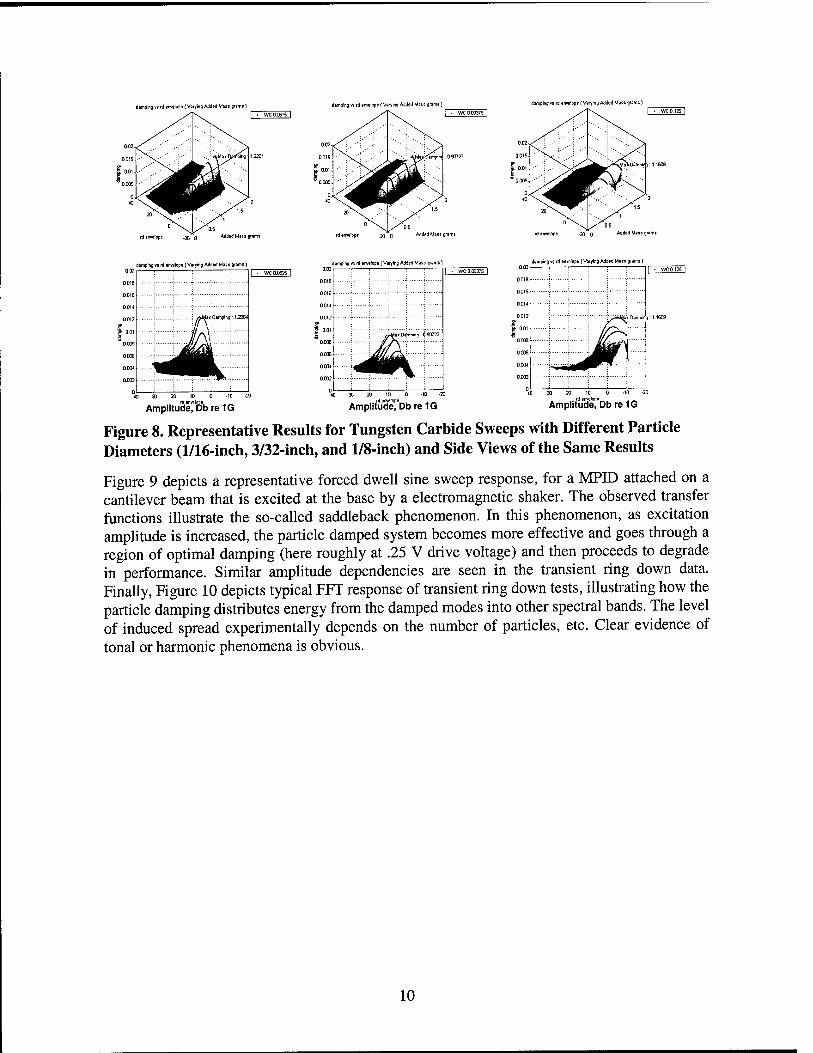
Figure 8. Representative Results for Tungsten Carbide Sweeps with Different Particle Diameters (1/16-inch, 3/32-inch, and 1/8-inch) and Side Views of the Same Results

Figure 9 depicts a representative forced dwell sine sweep response, for a MPID attached on a cantilever beam that is excited at the base by a electromagnetic shaker. The observed transfer functions illustrate the so-called saddleback phenomenon. In this phenomenon, as excitation amplitude is increased, the particle damped system becomes more effective and goes through a region of optimal damping (here roughly at .25 V drive voltage) and then proceeds to degrade in performance. Similar amplitude dependencies are seen in the transient ring down data. Finally, Figure 10 depicts typical FFT response of transient ring down tests, illustrating how the particle damping distributes energy from the damped modes into other spectral bands. The level of induced spread experimentally depends on the number of particles, etc. Clear evidence of tonal or harmonic phenomena is obvious.

10

Eight 0.125 inch tungsten carbide particles, 0.19 len x 0.5 dia cavity

"^^^"^^^j^^ °^'^""^^.

0.2

Driving Voitage (V) 0.1 25 Frequency (Hz)

Figure 9. Forced Sine Sweep Test Results for MPID Illustrating the Saddleback Phenomena

Response 5. FFT : 10

100 200 300 400 500 Frequency

700

Figure 10. Representative Fast Fourier Transforms (FFT) Showing Measured Frequency Content for Three Test Cases Frequency, Hz

sively More Particles

11

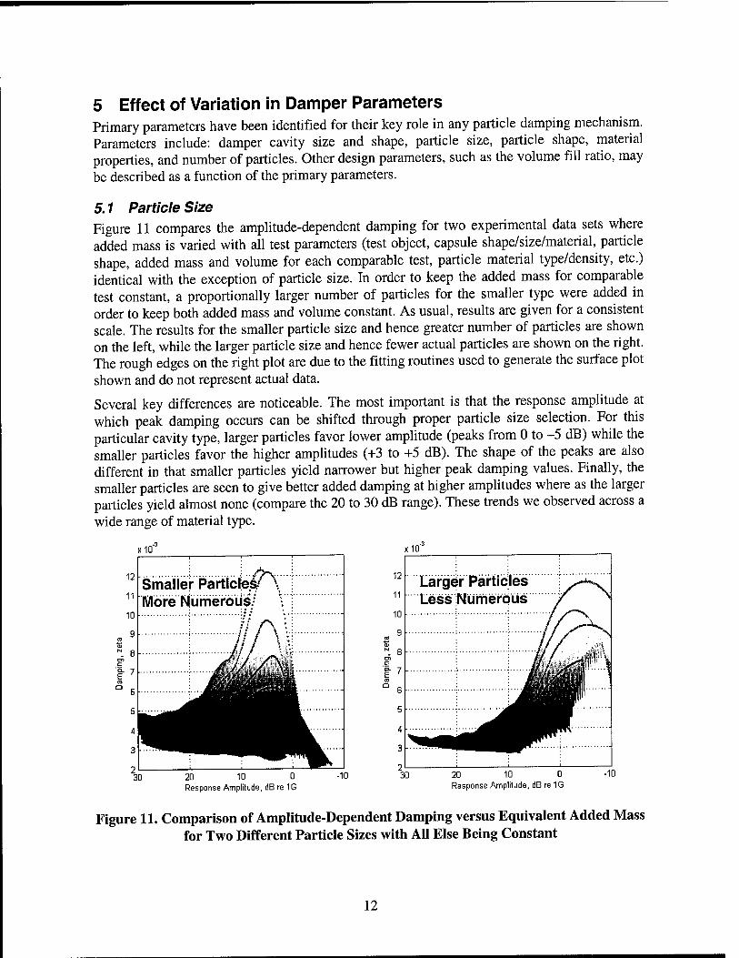
5 Effect of Variation in Damper Parameters Primary parameters have been identified for their key role in any particle damping mechanism. Parameters include: damper cavity size and shape, particle size, particle shape, material properties, and number of particles. Other design parameters, such as the volume fill ratio, may be described as a function of the primary parameters.

5.1 Particle Size Figure 11 compares the amplitude-dependent damping for two experimental data sets where added mass is varied with all test parameters (test object, capsule shape/size/material, particle shape, added mass and volume for each comparable test, particle material type/density, etc.) identical with the exception of particle size. In order to keep the added mass for comparable test constant, a proportionally larger number of particles for the smaller type were added in order to keep both added mass and volume constant. As usual, results are given for a consistent scale. The results for the smaller particle size and hence greater number of particles are shown on the left, while the larger particle size and hence fewer actual particles are shown on the right. The rough edges on the right plot are due to the fitting routines used to generate the surface plot shown and do not represent actual data.

Several key differences are noticeable. The most important is that the response amplitude at which peak damping occurs can be shifted through proper particle size selection. For this particular cavity type, larger particles favor lower amplitude (peaks from 0 to -5 dB) while the smaller particles favor the higher amplitudes (+3 to +5 dB). The shape of the peaks are also different in that smaller particles yield narrower but higher peak damping values. Finally, the smaller particles are seen to give better added damping at higher amplitudes where as the larger particles yield almost none (compare the 20 to 30 dB range). These trends we observed across a wide range of material type.

xlO xlD

^ 8

e (0 Q

4

3

2 30

1 1 1

\ \ />v '■■

Smaller Particfe^ \ ; More Numerous/

i- ji / \ '•

: Jl^^^^M

IVli:: 20 10 0 Response Amplitude, dB re 1G

-10 20 ID 0 Response Amplitude, dB re 1G

Figure 11. Comparison of Amplitude-Dependent Damping versus Equivalent Added Mass for Two Different Particle Sizes with All Else Being Constant

12

Total particle mass appears to have a fairly significant effect on damping for both single particle and multiple particle dampers. Increasing the mass tends to increase damping. Conversely, decreasing the mass tends to reduce damping. As might be expected, changes in the total particle mass can lead to a fairly significant shift in the frequency of peak response.

5.2 Dependence of Observed Behavior on Orientation witli Gravity Figure 12 compares the variation in achieved damping for nearly identical particle damping treatments in a fixed capsule. All major test parameters are identical (i.e., test object, capsule type/size, material, particle size, etc.) except for the orientation of the test object relative to the local quasi-static acceleration field. As indicated by the small cartoons on each figure, the plot on the left corresponds to the case where the excitation is not aligned with the local quasi-static acceleration field, and the one on the right corresponds to the aligned test condition. There are several distinct differences in behavior.

For example, the damping for the aligned direction case achieves a higher added damping (2.44 percent zeta versus 2.17 percent) but this is not the whole story. Perhaps the most striking difference is how consistently and sharply the damping turns off once the response levels drop below 1 G (or 0 dB on the plots) for the aligned case. Another more subtle difference is for the best performing damping treatment of each case the response amplitude range over which damping is added at the 2 percent damping is about identical in each case. At 1.5 percent level, the not aligned case is favored slightly, and favored quite strongly at the 1 percent damping level. Also the extracted ring down profiles versus added mass are more consistent for the aligned case.

A key conclusion that can be drawn from these results is that the direction in which the local quasi-static acceleration field acts can play a large roll in determining at which response amplitude particle damping will turn off and it also helps set the level of damping that can be achieved.

Not Aligned 0.D25

Aligned

10 6 0 Response Amplitude, dB re 1G


Figure 12. Comparison of Amplitude-Dependent Damping versus Added Mass for Two Different Orientations of the Test Object Excitation versus Local Quasi-Static

Acceleration Field

13

5.3 Dependence on Material Parameters Figure 13 compares the amplitude-dependent damping for two experimental data sets where the number of added particles, and hence added mass, is varied with all test parameters (test object, capsule shape/size/material, particle size/shape, number of particles for each comparable test, material type/density, etc.) being identical with the exception of a relatively minor variation in tested material alloy. The material on the left was SS-315. The material on the right was SS- 304. While they both show similar trends for increased performance with added particle count/mass, the one on the left is clearly superior in that it achieves smoother and higher damping levels for all numbers of added particle. The amplitude of peak damping also does not seem to vary as much. The high amplitude behavior (i.e., above 20 dB) for both types is similar, as is the fact that they turn off around 0 dB.

Alloy 1

H

\ / \ \

i i i : '■'^ 20 15 10 5 0

Response Amplitude, dB re 1G

20 15 10 5 0 Response Amplitude. dB re 1G

Figure 13. Comparison of Amplitude-Dependent Damping versus Added Mass for Two Experimental Data Sets for the Same Base Material but Slightly Different Alloys

14

6 Test System Overview A wide range of test rigs (eight basic types) were developed to experimentally investigate various aspects of particle damping behavior. The name and general purpose of each of the test systems is listed in Table 1. Pictures of each of the test system are gathered in Figure 14. Highlights of the test results for each test system are discussed in the following sections.

Table 1. Test Systems

Basic Test Rigs Name

Basic Beam Tester Vertical Config. Horizontal Config.

"Big Beam"

Mass-Spring-Damper (MSP) Approximation

Purpose Measure basic particle damping performance over a wide range of • Particle materials/shapes/sizes/fill ratios • Capsule sizes/shapes/materials • Orientation of excitation versus gravity

Excitation methods. Scaled up version of basic beam tester. Used to experimentally check scaling laws for modal mass ratio, particle and capsule sizes, etc. Also used to study the effects of capsule wall thickness. Study mass ratio, stiffness, and inherent damping effects in a controlled manner. Also ensures linear motion.

Temperature Chamber Sweeps Kiln Test Rig

Temperature Sensitivity Measure the effect of range of intermediate temperatures (-94 to +365 °F) on the behavior of particle damping Measure the effect of high temperatures (70 to 850 T) on the behavior of particle damping.

Panel Test Rig

High-Temp Material Test Rig

Higher Order Structure Test Rigs Demonstrate particle damping can work on more complicated structures and study design approaches. Demonstrate particles damping can work on complicated structures and at high temperature.

Duration Tester

Other Begin preliminary measurements of durability of particle damping treatments.

15

'■.i':liJv\v:',Jik

Figure 14. Overview of tlie Various Test Systems, Left to Right Working Down from Upper Left: Basic Beam (Horizontal Configuration), Oven, Panel, Kiln, Big Beam,

Duration Test Rig, Mass-Spring-Damper

16

6.1 Basic Beam Tester Most of the experimental studies of particle damping behavior were performed with the test object shown in Figure 15. It consisted of a well-clamped cantilever beam. Per the standard test approach experimental displacement or acceleration data is recorded over the ring down time. A Hilbert transform is used to capture the envelope of this data. The envelope is subsequently fit with splines over multiple discrete, but piecewise continuous, regions. These spline fits can then be used to calculate the local slope of the ring down, which is related to the damping at that amplitude. This approach is similar to the log decrement method, but is less sensitive to noise.

Well over 2,000 individual ring down tests of different combinations of particles, capsules, and orientation relative to gravity have been performed with this test setup. Representative results from some of these tests are shown in Figure 16. The data compares the differences in behavior for the different amounts of particles in the same capsule. The test setup has been used to study the effects of the following.

Particles

• Different materials • Different heat treats on otherwise similar materials • Particle size • Particle shape • Particle fill ratio • Number of particles (single versus multiple)

Capsules

• Capsule diameter • Capsule length • Capsule material (limited)

Orientation of excitation relative to local gravity

• Aligned • Not aligned

Excitation approaches

• Air pulses (insufficient excitation) • Electrodynamic shaker (used for sine sweeps and forced response only) • Manual displacements or tapping.

17

Figure 15. Experimental Test Setup Used for Basic Particle Damping Characterization (in the Excitation Aligned with Gravity Orientation)

xlO



Figure 16. Experimental Results Comparing Amplitude-Dependent Damping for Multiple Particle Dampers with (left) Numerous, Smaller Particles versus (right) Fewer, Larger

Particles

6.2 Big Beam The objective of this test hardware was to gather data with much larger dampers to determine if/how the data for smaller capsules scaled to that of the larger particle dampers, and if larger dampers could produce similar performance as that of the smaller ones. The experimental apparatus consisted of the beam, two identical particle damper assemblies, and the instrumentation and data acquisition system. The host structure used was a large, vertically oriented, cantilevered beam. The beams dimensions were 4 by 1 inches with a free length of 42-9/16 inches. Two independent capsule holders could accommodate capsules that ranged from 1.1,1.6, and 2.1 inches in inner diameter, and lengths from 0.6 to 4.1 inches long.

An initial sweep with the largest ID capsule and five different particle diameters revealed that the longest capsule and the second largest particle size yielded the best results. More detailed tests with this capsule revealed that, unlike the smaller damper capsules which generally had

18

peak damping about 50 percent full, these capsules had best damping when nearly 100 percent full. Also, after crossing the 50 percent fill ratio, the behavior of the damping changed slightly, as shown in Figure 17. The plot in Figure 17 shows a specific case where the number of particles was increased from 50 to 176 particles using 7/16-inch stainless steel balls. The cavity was essentially 100% full with 176 balls.

The larger physical size of the damper capsules also allowed the initial study of the effects of different wall and cap thickness. For the limited tests performed, it was seen that both wall thickness and cap thickness can influence the observed damping, actually improving it in the measured test cases (6.5% peak damping for thick case, 9.0% peak for the thin/thin case).

6/13/01 Large Particle Damper Resulls 4.1' X 2.1 Thick Wall Capsule

7/16" SS Bans

^ 50

^ 70

-' ^

BO 90

100 - ■ 110 - • 114 ... - izo -. ■ 130

^^ 140 ■ ■ 150 160 170

176

Rjngifown Ampfilude, dB re 1 G

Figure 17. Representative Test Results for the Big Beam Tester Where Increase in the Number of Particles (Up to Nearly 100 Percent Full) Showed Increase in Damping

6.3 Mass Spring Damper Approximations Using modified hardware taken from previous projects and additional custom test components, a test apparatus which served as an engineering approximation of the standard linear, single- degree-of-freedom (SDOF) MSD system was created. Using this test apparatus and a fixed particle damping treatment, it was then possible to individually study the effects of variations in stiffness, mass, and mass ratios as well as, to a limited extent, see how particle damping performed in conjunction with other damping treatments.

This test setup was useful, as the majority of the experimental tests described in this document were on cantilevered beams or more complex structures. This made it difficult to conclusively decouple the effects of variations in mass ratio, stiffness, etc. There was also the slight added complication of the fact that, at least for the cantilever beam cases, the path of the capsule motion is not truly linear but follows a curved profile set by the length of the beam. This adds another discrepancy between experimental work and explicit modeling results. Having a linear spring element reduces this discrepancy and provides the ability to vary mass and stiffness values.

The MSD test hardware is shown in Figure 18. It consisted of a

19

Standard test capsule holder and spiral flexure end clamp Two or more spiral flexures Spacer housing and spiral flexure end caps Central spacing element Spiral flexure end clamp Accelerometer mount Accelerometer Additional moving mass elements

Figure 18. Mass-Spring-Damper Approximation Setup

Stiffness Elements Stiffness was provided by spiral flexure. Each flexure provides roughly 12,400 N/m of stiffness (equivalent to 70.8 Ibf/in). The total system level stiffness is then N x 12,400 N/m where N is the number of implemented flexures. The minimum number for N is 2, maximum is 10 but 6 was the maximum which yielded good test results

Moving Mass The basic structure of the MSD hardware created an inherent baseline moving mass of approximately 170 grams. In order to perform tests where the mass and stiffness increased in equal amounts (hence keeping the natural frequency the same but changing the mass ratio) it was necessary to have custom mass elements made. They bolted onto the outside of the MSD for ease of integration. Four additional masses corresponding to the 4 additional stiffness states (N = 3,4, 5, 6) were made. The mass increment turned out to be 82.8 grams.

Inherent Damping Aerodynamic damping was one source of damping for the two-flexure case. When more than two flexures were used, interlaminar friction between neighboring flexures contributed significantly more damping. Inherent damping levels of approximately 0.4 percent to 2.0 percent zeta were experimentally observed. At first, these large levels of inherent damping were feared to create too high of a 'damping noise floor' but later it was seen that this was not the case.

Particle Damping Treatment

20

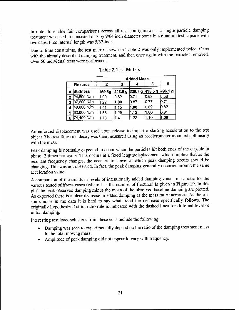
In order to enable fair comparisons across all test configurations, a single particle damping treatment was used. It consisted of 7 by 9/64 inch diameter bores in a titanium test capsule with two caps. Free internal length was 5/32-inch.

Due to time constraints, the test matrix shown in Table 2 was only implemented twice. Once with the already described damping treatment, and then once again with the particles removed. Over 50 individual tests were performed.

Table 2. Test Matrix

Added Mass Flexures 2 3 4 5 6

# Stiffness 169.3g 243.9 g 329.7 g 415.5 g 496.1 g

2 24,800 N/m 1.00 0.82 0.71 0.63 0.58

3 37,200 N/m 1.22 1.00 0.87 0.77 0.71

4 49,600 N/m 1.41 1.15 1.00 0.89 0.82

5 62,000 N/m 1.58 1.29 1.12 1.00 0.91

6 74,400 N/m 1.73 1.41 1.22 1.10 1.00

An enforced displacement was used upon release to impart a starting acceleration to the test object. The resulting free decay was then measured using an accelerometer mounted collinearly with the mass.

Peak damping is normally expected to occur when the particles hit both ends of the capsule in phase, 2 times per cycle. This occurs at a fixed length/displacement which implies that as the resonant frequency changes, the acceleration level at which peak damping occurs should be changing. This was not observed. In fact, the peak damping generally occurred around the same acceleration value.

A comparison of the trends in levels of intentionally added damping versus mass ratio for the various tested stiffness cases (where k is the number of flexures) is given in Figure 19. In this plot the peak observed damping minus the mean of the observed baseline damping are plotted. As expected there is a clear decrease in added damping as the mass ratio increases. As there is some noise in the data it is hard to say what trend the decrease specifically follows. The originally hypothesized strict ratio rule is indicated with the dashed lines for different level of initial damping.

Interesting results/conclusions from these tests include the following.

• Damping was seen to experimentally depend on the ratio of the damping treatment mass to the total moving mass.

• Amplitude of peak damping did not appear to vary with frequency.

21

Added Mass Case

Figure 19. Representative MSD Test Results

6.4 Temperature Chamber Sweeps The purpose of this test setup was to enable testing of variable capsule geometries and particle fills in the standard cantilever beam over a wide temperature range (-70 to +185 °C, -94 to 365 T). This corresponds to a 255 °C (459 T) total temperature range. It was intended to complement the high-temperature kiln (described in Section 6.5) in that it enabled testing to very cold levels well below room temperature and tighter temperature control at elevated temperature up to the environmental chamber's upper limit.

The test setup consisted primarily of the standard cantilever beam. As the test beam was now inside of an environmental chamber, an electromechanical push-pull solenoid system was used to create the required initial displacement and release. This turned out to provide a very repeatable excitation.

For the majority of the performed tests, a titanium capsule with seven through holes containing seven tungsten carbide spheres 1/8-inch in diameter was used. The standard data acquisition system and postprocessing approach using Hilbert transforms of the ring down was applied. Representative results are shown in Figure 20 where damping (percent zeta) is plotted versus amplitude (dB relative to 1 G). Comparative baseline curves that remain below 0.4 zeta represent tests at each temperature where no additional damping was intentionally added. They are shown in solid colors. The particle damping measurements for the given temperatures are dashed.

While there is some variability in the baseline measurements and in the damped measurements, the seen changes do not correlate to changes in temperature, and are believed to represent inherent noise in the test/data extraction process. The overall scale of observed damping for the intentionally damped cases, versus the baseline cases (i.e., 3 percent intentional versus 0.35 percent baseline peak damping) is significant. The key conclusion is that very little sensitivity to temperature was seen over the test range.

22

Baseline and Damping Treatment

-68,1 14.2 25

72.3 3

\^ 111.2 132.2 iei.8 66.8

2.5

''"■•\

- -15.6 — 27 -- 71.2

111

r - W'' 135.8

i ;c\ 180.9

|l.5

1 "\ ill O.b

. ~:--2Sa#^ Amplitude,db.rellg

vBH^K^^i%' ■ ^;^-11 uH^H^^HkjA HF ^^HI^^^^^^ £^ ^^M 'w ^t{ ^^^I^^HI

BI^^^MI ■" ■ "lyB ■^^^5^ ̂ ^■■i^^Qf^H ^^^^^1 MBMBBIMI

Figure 20. Representative Baseline and Damped Experimental Test Results at Various Temperatures and the Test Setup Installed in the Environmental Chamber

6.5 Kiln Test Rig The ultimate goal of this testing effort was to see if the damping characteristics of an impact or particle damper would change with temperatures of up to 1,000 T. The temperature limitations of transducers prevented the experimenters from collecting data up to that temperature. Reliable data was collected from room temperature up to 850 T.

The tube-furnace shown in Figure 21 was modified to house a stainless-steel fixture and cantilever beam. The excitation was performed using a spring-loaded plunger system.

23

Figure 21. High-Temperature Test Rig

Thermal expansion contributed significantly to problems and irregularities encountered during initial testing. The original design of the test apparatus had to be modified slightly (Bellville washers) in order to limit the effects of thermal expansion of the hardware on the measured data. This is shown in Figure 22. It is believed that most of these problems were overcome. Once these issues were removed, it was experimentally demonstrated that particle damping can be applied to applications up to at least 850 T. In some cases, some sensitivity to temperature was seen (damping actually improved). Representative data is shown below for a multiple particle cavity setup where, again, the post processing approach using Hilbert transforms of the ring down was applied. Representative results at various temperatures are shown in Figure 23 where damping (percent zeta) is plotted versus amplitude (dB relative to 1 G). While the data are noisy, there are no clear temperature dependencies. The baseline curve is a room temperature test with no particles in the cavity.

24

Large Bellville

Housing

Particles

Small Bellvilles

Jam Nut

Sleeve

Floating Wall End Cap-

Figure 22. High-Temperature Particle Damper Assembly

Inconel 718 Capsule, 68 3/32 WC Balls, .5" Long x .447' ID 316 Slee\« Temperature Sweep {deg F)

88 184 279 357

483 551 --649 -- 750

856 baseline

5 10 15 Ringdown Amplitude, dB re 1 G

20

Figure 23. Representative Baseline and Damped Experimental Test Results at Designated Temperatures

25

6.6 Duration Tester The objective of this test hardware, shown below in Figure 24, was to detemoine if MPIDs undergo any significant wear and/or changes in damping characteristics as they are subjected to many cycles. The experimental apparatus consisted of the particle damper itself, a cantilevered beam host structure, excitation device, and data acquisition system. Two different particle dampers were tested. The testing performed revealed that the dampers did undergo significant wear over about 6 days of continuous operation. From a product standpoint, this could be a serious concern and design challenge. Fortunately, the wear that did occur tended to increase the performance of the damper.

Figure 24. Cavity Pitting and the Durability Test Rig

26

7 Theoretical Background The particle damper is conceptually a relatively simple device. However, the behavior of the particle damper is highly nonlinear and energy dissipation, or damping, is derived from a combination of loss mechanisms. The relative effectiveness of these mechanisms changes based on various system parameters. In the first subsection, loss mechanisms present in the particle damper are reviewed.

In the next subsection, the incorporation of these loss mechanisms into the mathematical model is discussed. The mathematical model has been developed based on the particle dynamics method. The utility of the particle dynamics method is derived from the ability to simulate contact interaction forces with a small number of parameters which capture the most important contact properties. One of the critical aspects for developing an accurate mathematical model is the selection of appropriate force-displacement relations.

Lastly, the incorporation of the particle dynamics method into an explicit finite element code is discussed. Contact detection algorithms are reviewed, along with the implementation of the force-displacement relations used to resolve the contact. Sample results and correlation of predicted results with measured experimental data are considered in Sections 4 and 5.

7.1 Particle Damper Loss Mechanisms Passive damping techniques attenuate the response of a vibrating structure by removing a portion of the vibratory energy. One method of removing the vibratory energy is to transfer the energy to a secondary system. Dynamic vibration absorbers function in this manner. Oscillations of the dynamic vibration absorber are created with a fraction of the energy creating the oscillations of the primary system. This mechanism is present in the particle damper in the form of the momentum transfer which occurs when the particles impact the cavity ends.

A second method of removing the vibratory energy is to dissipate the mechanical energy in the form of heat or noise. Viscoelastic and viscous damping dissipate energy in the form of heat created when the viscoelastic material or viscous fluid undergoes shear. Friction damping also dissipates energy in the form of heat which is created due to the relative motion between two contacting surfaces. In particle dampers, friction exists when relative sliding (or, to a much lesser degree, rolling) motion occurs between individual particles in contact or between particles in contact with the cavity walls. Viscoelastic behavior also is present in the particle dampers due to impacts with nonunity coefficients of restitution (i.e., impacts which are not perfectly elastic).

For convenience, the loss mechanisms present in the particle damper can be grouped into "external" and "internal" mechanisms. "External" mechanisms involve friction and impact interactions between the particles and the cavity. "Internal" mechanisms involve friction and impact interactions between the individual particles. The relative effectiveness of these mechanisms changes based on various system parameters. For example, at low excitation levels or for relatively long cavity lengths, insufficient energy may exist to create impacts between the particles and the cavity ends. Under such circumstances, any dissipation would be due solely to any sliding or rolling friction between the particles and the cavity or interactions between the individual particles. For higher excitations or shorter cavity lengths, however, losses due to impacts between the particles and the cavity ends may dominate the overall dissipation.

27

Incorporation of the various loss mechanisms into the mathematical model will be performed through the definition of appropriate force-displacement relations.

7.2 Force-Displacement Relations In the following paragraphs, the force-displacement relations used to account for the contact interactions between the individual particles and between the particles and the cavity walls are considered. It has been assumed that the particle dampers consist of spherical particles of the identical material. Consider a typical impact of two spherical particles, i and j, with radii Ri and Rj, with the particle centers separated by a distance, dij, as shown in Figure 25.

Particle i

Particle j

Figure 25. Typical Particle-Particle Impact Parameters

These two particles interact if their approach, a, is positive. The approach can be defined according to the following equation

a = (Ri+Rj)-d..

In this case, the colliding spheres feel a force, F, equal to the following

F = F^-n^+F^-nS

(1)

(2)

where n^ and n^ are the unit vectors in the normal and shear directions, respectively, and F^ and F^ refer to the normal and shear forces. The normal force acting between colliding spheres can be broken down into an elastic portion and a dissipative portion as follows:

F^=F& + F(1) (3)

The following paragraphs discuss the elastic and dissipative portions of the normal force, the shear force, and the forces due to particle-cavity impacts.

28

7.2.1 Elastic Portion of Normal Force Expressions for the elastic portion of the normal force are based on Hertz's theory of elastic contact [3-4]. Hertz derived expressions for the stress between contacting bodies based on the basic equations of elasticity and on the geometries of the contacting bodies. More specifically, Hertz's expressions are an extension of the work of Boussinesq [5], who used the theory of potential to establish a method to determine the stresses and displacements resulting due to surface tractions on an elastic half-space. The derivation of Hertz's theory is discussed briefly in the following paragraphs. Complete derivation of Hertz's theory can be found to various levels of detail in a number of classical elasticity texts [6-8].

For elastic bodies in contact, Hertz determined that the contact area is generally elliptical and assumed that each body could be regarded as an elastic half-space loaded over a small elliptical region of its plane surface. This assumption implies that the dimensions of the contact area must be small compared with the dimensions of each body and with the relative radii of curvature of the surfaces. These assumptions are necessary to ensure that: (1) the boundaries of the bodies do not significantly affect the stresses in the contact zone; (2) the portions of the bodies outside of the contact zone can be roughly approximated as an elastic half-space; and, (3) the strains remain sufficiently small that the linear theory of elasticity applies. Hertz also assumed that the contact is frictionless such that only normal pressures are transmitted through the contact.

For two elastic bodies in contact, Hertz showed that the total normal force is related to the approach via the power law

F(^) = Ca- (4)

where C is a constant which depends on the elastic properties of the materials and on the local curvature of the bodies. For the case of two contacting spheres with identical properties, a circular contact area with radius, a, results. Hertz showed that Equation 4 becomes

where

R=hH (6) (Ri+Rj)

and E and v are the Young's modulus and Poisson's ratio of the spheres, respectively. The approach and contact circle radius are related as follows:

.,2

(7) R

Equation 5 also holds for two impacting spheres, provided that the duration of the collision is long compared with the first fundamental mode of vibration in the spheres [9].

7.2.2 Particle-Cavity Relations In addition to particle-particle impacts, particle-cavity impacts also can occur. Saluena, et al. [10] resolve particle-cavity impacts by using a fixed layer of particles along the cavity walls. A

29

similar procedure has been used in some experimental efforts [11]. This assumption may be appropriate for simulating behavior such as granular flow down an inclined chute, where there may exist a thin layer of particles which essentially remain in contact with the cavity wall. However, particles in a damper often may collide with the cavity walls rather than with other particles. As a result, particle-cavity force-displacement relations are required. Although the complete derivations are not shown here, the particle-cavity force-displacement relations can be formulated by modifying the particle-particle force-displacement relations to account for the material properties of the cavity and the local curvature. For simplicity, it has been assumed that the cavity walls are flat and rigid. Particle-cavity relations for flat cavity walls are derived from the particle-particle relations by assuming the radius of curvature for the cavity walls goes to infinity. Note that this assumption is valid since the flat surface more closely represents the Boussinesq solution for the surface tractions on an elastic half-space on which Hertz's theory is based. Under the assumption of rigid walls, the effective modulus simply becomes the particle modulus.

7.2.3 Dissipatlve Portion of Normal Force For damping studies, it is important to model the dissipative portion of the normal force. If the granular material in the particle dampers were to behave in a gas-like manner, it would be possible to resolve particle-particle and particle-cavity impacts instantaneously using a coefficient of restitution or similar parameter. However, the granular material in particle dampers tends to behave more like a liquid or solid in that enduring contacts occur. As a result, the use of a coefficient of restitution is no longer appropriate and any dissipation must be accounted for in the force-displacement relations.

Studies on the coefficient of restitution for the impact of two spheres have demonstrated that energy is dissipated due to the viscoelastic behavior of the sphere material [12]. Finite element analyses of a sphere impacting a rigid plate have been performed to investigate the significance of viscoelasticity. An axisymmetric model, shown in Figure 26, has been used for the analyses. The model contains 16,000 4-node bilinear axisymmetric solid elements (CAX4 elements in ABAQUS) to accurately capture the contact behavior. Figure 27 shows the region where the spherical particle initially contacts the rigid wall.

30

Figure 26. Axisymmetric Model of Spherical Particle and Rigid Wall

Figure 27. Region Where Spherical Particle Initially Contacts Rigid Wall

To validate the finite element model, initial analyses have investigated the impact of an elastic sphere of radius 0.0625 inch with a rigid wall and have been compared to predicted results

31

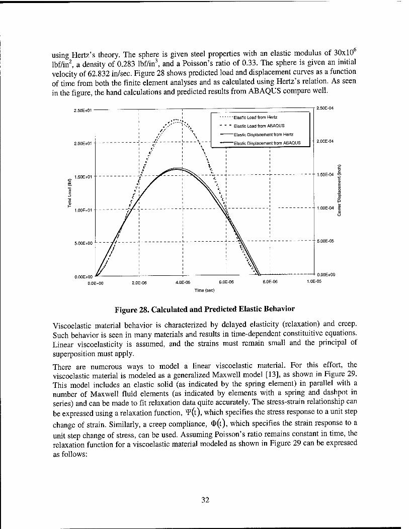
using Hertz's theory. The sphere is given steel properties with an elastic modulus of 30x10 Ibf/in^ a density of 0.283 lbf/in^ and a Poisson's ratio of 0.33. The sphere is given an initial velocity of 62.832 in/sec. Figure 28 shows predicted load and displacement curves as a function of time from both the finite element analyses and as calculated using Hertz's relation. As seen in the figure, the hand calculations and predicted results from ABAQUS compare well.

2.50E+01

2.00E+01

1.50E+01 ■-

1.00E+01

5.00E+00

O.OOE+00

O.OE+00

1 1 — 1 —i— 1

1 1

, ,.■• 1 \ 1 „,'' ' "•

Elastic Load from Hertz

" " " Elastic Load from ABAQUS

1 ,• 1 V 1 // 1 \

1 •-■ 1 \

T /^ ^ ^^ » 1 / 1 \

// ;

»* '

1 1

-•

2.50E-04

-■2.00E-04

1.50E-04 ■■=■

1.00E-04

5.00E-05

O.OOE+00

2.0E-06 4.0E-06 6.0E-06

Time (sec)

8.0E-06 1.0E-05

Figure 28. Calculated and Predicted Elastic Behavior

Viscoelastic material behavior is characterized by delayed elasticity (relaxation) and creep. Such behavior is seen in many materials and results in time-dependent constituitive equations. Linear viscoelasticity is assumed, and the strains must remain small and the principal of superposition must apply.

There are numerous ways to model a linear viscoelastic material. For this effort, the viscoelastic material is modeled as a generalized Maxwell model [13], as shown in Figure 29. This model includes an elastic solid (as indicated by the spring element) in parallel with a number of Maxwell fluid elements (as indicated by elements with a spring and dashpot in series) and can be made to fit relaxation data quite accurately. The stress-strain relationship can be expressed using a relaxation function, *F(t), which specifies the stress response to a unit step

change of strain. Similarly, a creep compliance, 0(t), which specifies the strain response to a unit step change of stress, can be used. Assuming Poisson's ratio remains constant in time, the relaxation function for a viscoelastic material modeled as shown in Figure 29 can be expressed as follows:

32

vF(t)=Eo+E,e- ■t/T, + £^6 -t/T, ... + E„e -t/T„

i=0

-t/ti , where — = 0 ^0

(8)

In Equation 8, the instantaneous modulus is represented as the sum of the Ei, and the elastic modulus at long times is represented by EQ. The moduli, Ei, and corresponding time constants, Ti, can be determined from complex modulus material properties, such as those obtained by testing in accordance with ASTM E756-93, "Standard Test Method for Measuring Vibration- Damping Properties of Materials" [14].

m ffl m

Figure 29. Maxwell Model for Viscoelastic Behavior

The time constants in Equation 8 are used to account for the behavior of the material during loading over various time periods or, equivalently, at various frequencies. From Hertz's theory, the time of maximum compression for an elastic impact of two spheres can be calculated. As a first approximation, the time to maximum compression can be thought of as a quarter cycle of sinusoidal loading. Thus, approximate loading frequencies can be calculated based on the time to maximum compression. The compression times for the impact of two identical elastic steel spheres at various impact velocities which might be expected in a typical particle damper have been calculated. Results from these calculations, along with the approximate period of a loading cycle and the approximate loading frequency are given in Table 3.

Table 3. Approximate Loading Frequencies for Various Impact Velocities

Impact Velocity

(in/s)

Time of Maximum

Compression (s)

Approximate Period

of Loading (s)

Approximate Loading

Frequency (Hz)

6.28x10"^ 1.72x10"^ 6.90x10"^ 1.45x10'^

6.28x10-^ 1.09x10-^ 4.35x10"^ 2.30x10^

6.28x10° 6.86x10-^ 2.75x10"^ 3.64x10"^

6.28x10' 4.33x10"^ 1.73x10-^ 5.77x10''

33

6.28x10^ 2.73x10-^ 1.09x10'^ 9.15x10^

6.28x10^ 1.72x10-^ 6.90x10"^ 1.45x10^

Using a three-parameter (EQ, EI , and i^) viscoelastic model, the relaxation function takes the

form

W{t)=E,+E,c'"" (9)

The equivalent loss factor, r), for a viscoelastic material with the relaxation modulus shown above is as follows:

E" Tl^

E' (10)

where E' and E" are the storage and loss moduli, respectively, and can be found as follows:

E' = E,+imJ F^KT)

(11)

E' = (cOTj ) fivj) (12)

with CO equal to the loading frequency in rad/s. Earlier work [12] indicates that the dissipation due to the deviatoric and dilatational strains are of similar magnitudes. As a result, the relaxation function is not broken into separate deviatoric and dilatational components or, equivalently, it is assumed that the Poisson's ratio remains constant.

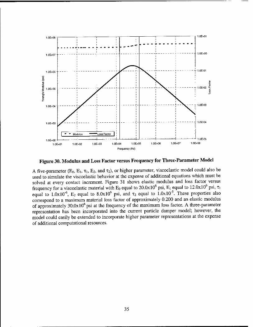
Figure 30 shows elastic modulus and loss factor versus frequency for a viscoelastic material with Eo equal to 24.0x10^ psi, Ei equal to 12.0x10^ psi, and Ti equal to 2.0x10'^ These properties correspond to a maximum material loss factor of approximately 0.200 and an elastic modulus of approximately 30.0x10^ psi at the frequency of the maximum loss factor. (Note that these properties are not representative of the typical intrinsic damping of steel, which may be much less than 0.200, but have been used for illustrative purposes.) The material has an instantaneous modulus of 36.0x10^ psi and a long-term modulus of 24.0x10^ psi. Based on the results shown inTable 3, it is likely that the majority of the impacts during a particle damper simulation will occur at frequencies between approximately 1.45x10"^ and 1.45x10 hertz. This range is shown in Figure 30.

34

1.0E+08

1.0E+07

1.0E+06

I 1.0E+05

1.0E+04-r

1.0E+03

1 .OE+02

......-•._— - > U -o - - <" , - -- + i i

V 1

1

A ^r 1 i- J

—

\

\ \ ^

1 1 1

1.0E+01

-- 1.0E+00

1.0E-01

-- 1.0E-02 "-

-- 1.0E-03

1.0E-04

1.0E-05

1.0E+01 1.OE+02 1.0E+03 1.0E+04 1.0E+05

Frequency (Hz)

1 .OE+06 1.0E+07 1.0E+08

Figure 30. Modulus and Loss Factor versus Frequency for Three-Parameter Model

A five-parameter (Eo, Ei, Ti, E2, and T2), or higher parameter, viscoelastic model could also be used to simulate the viscoelastic behavior at the expense of additional equations which must be solved at every contact increment. Figure 31 shows elastic modulus and loss factor versus frequency for a viscoelastic material with Eo equal to 20.0x10^ psi, Ei equal to 12.0x10 psi, Xi equal to 1.0x10^ E2 equal to 8.0x10^ psi, and T2 equal to 1.0x10"^ These properties also correspond to a maximum material loss factor of approximately 0.200 and an elastic modulus of approximately 30.0x10^ psi at the frequency of the maximum loss factor. A three-parameter representation has been incorporated into the current particle damper model; however, the model could easily be extended to incorporate higher parameter representations at the expense of additional computational resources.

35

1.0E+08 T

1.0E+07-r

1.0E+01

1.0E+00

1.0E+02 1.0E-05

1.0E+01 1.0E+02 1.0E+03 1.0E+04 1.0E+05 1.0E+06 1.0E+07 1.0E+08

Frequency (Hz)

Figure 31. Modulus and Loss Factor versus Frequency for Five-Parameter Model

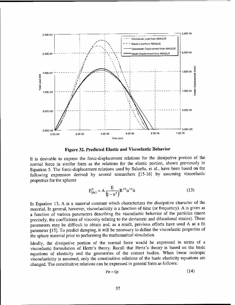
Using the existing finite element model, ABAQUS analyses have been performed to assess the effect of using viscoelastic properties for the spheres. The steel sphere has been given the three- parameter viscoelastic properties as shown in Figure 30. Figure 32 shows predicted load and displacement as a function of time when elastic properties are used and when viscoelastic properties are used. Note that when viscoelastic properties are used, a lesser maximum total force is predicted, with the peak force occurring prior to the peak displacement. After the peak displacement, the displacements tend to remain larger longer and require a longer time to return to zero.

36

2.50E+01 -1 —1— i

1 ,.'""'■.

1 «' h » 1 J iV

Viscoelastic Load from ABACUS

■ ■ ■ Elastic Load from ABAQUS

Elastic Displacement from ABAQUS 2.00E+01 ■

1 '/ 1 - » 1 -'» 1 ". »

l/ 1 \ \ 1.50E+01 •

"""'V >^ 1.00E+01 -

'7^ 1 %, 5.00E+00 ■

/I i 1%^

2.50E-04

2.00E-04

1.50E-04 -

1.00E-04

5.00E-05

O.OOE+00

O.OE+00 2.0E-06 4.0E-06 6.0E-06

Time (sec)

8.0E-06 1.0E-05

Figure 32. Predicted Elastic and Viscoelastic Behavior

It is desirable to express the force-displacement relations for the dissipative portion of the normal force in similar form as the relations for the elastic portion, shown previously in Equation 5. The force-displacement relations used by Salueiia, et al., have been based on the following expression derived by several researchers [15-16] by assuming viscoelastic properties for the spheres

THN _ A_^__T?1'2 1/2- (13)

In Equation 13, A is a material constant which characterizes the dissipative character of the material. In general, however, viscoelasticity is a function of time (or frequency). A is given as a function of various parameters describing the viscoelastic behavior of the particles (more precisely, the coefficients of viscosity relating to the deviatoric and dilatational strains). These parameters may be difficult to obtain and, as a result, previous efforts have used A as a fit parameter [15]. To predict damping, it will be necessary to define the viscoelastic properties of the sphere material prior to performing the mathematical simulation.

Ideally, the dissipative portion of the normal force would be expressed in terms of a viscoelastic formulation of Hertz's theory. Recall that Hertz's theory is based on the basic equations of elasticity and the geometries of the contact bodies. When linear isotropic viscoelasticity is assumed, only the constituitive relations of the basic elasticity equations are changed. The constituitive relations can be expressed in general form as follows:

Pa = Qe (14)

37

For viscoelasticity, P and Q are linear operators in the time variable which express the viscoelastic behavior of the material. These operators may include differential operators, integral operators, or any other equivalent means of expressing viscoelastic behavior. For the three-parameter viscoelastic model used for this effort, the following applies:

P = l (15)

Q = ^>(i)=E,+E,e-''' (16)

and the constituitive relation (relating the normal stress and normal strain) can be written as follows:

^ = ^(?> = (Eo+E,e-''^'> (17)

The assumptions inherent in the Hertz solution also must not be violated. In particular, these assumptions must ensure that: (1) the boundaries of the bodies do not significantly affect the stresses in the contact zone; (2) the portions of the bodies outside of the contact zone can be roughly approximated as a viscoelastic half-space; and, (3) the strains remain sufficiently small that the linear theory of viscoelasticity applies. To ensure the above conditions, the dimensions of the contact area must be small compared with the dimensions of each body and with the relative radii of curvature of the surfaces.

Pao [17] was one of the first to attempt to extend the Hertz solution to include linear viscoelasticity. Pao took the Laplace transform of the viscoelastic equations (i.e., the basic elasticity equations with a viscoelastic constituitive equation), to remove the time variable and yield an elastic problem in terms of transformed variables. This solution method is valid if the regions over which different types of boundary conditions are prescribed do not vary during the time under consideration. However, for the special case of the impact of viscoelastic spheres, these regions vary and this approach fails since for some points on the surface, neither the traction nor the displacement is known throughout the history of the problem, so the transform of neither can be determined [18].

Radok [19] suggested an alternative approach of taking a one-parameter family of solutions of the elastic problem in the time domain, with the same boundary conditions as the viscoelastic problem, and replacing the elastic constants with the appropriate viscoelastic operators in the expressions for the stress components. This procedure can permit the manipulation of the elastic constants in the determination of the elastic solution to involve procedures which are not valid for operators, or which lead to the introduction of new functions in the operator case. As a result, the significance of any solution must be checked, often by changing the initial formulation so that a direct transform attack is available. Using this alternative approach, Lee and Radok [18] have shown that, as long as the contact area is increasing, a simple relation for the normal force can be derived by replacing the elastic modulus in Hertz's relation (Equation 5) with the relaxation function for the sphere material. Substituting the relaxation function into Hertz's relation and recognizing that the contact radius also is a function of time, the total normal force (i.e., the normal force due to the combined elastic and dissipative components) at any time can be expressed as follows:

3 1 f„,/ .Ad ^"«=^F^!"('-''>s^^(''^*' "^^

38

Substituting the relation in Equation 7 for the contact radius, the derivative in Equation 18 can be evaluated. Equation 9 also can be substituted for the relaxation function yielding, as follows:

■n 1/2 t n

"(0=7;^|EE.e-('-''^^'a(t'rd(t>' (19)

For greater utility, it would be beneficial to express Equation 19 in incremental form such that the total load at any time can be calculated based only on information from the previous time. Otherwise, it will be necessary to retain the entire loading history. The contact force at a time equal to the original time, t, plus an additional increment in time, At, can be expressed as follows:

r> 1/2 t+At n

FN(t + At)=-J-^ J XEie-(-^-'>-a(t'rd(t')dt' (20) (1-0) jo i=o

The integral in Equation 20 can be broken into two parts, one from time 0 to t, and the second from time t to t+At, as follows:

,1/2 ft n '+^' n FN(t + At)=7^ |j:E,e--^'a(t7'^d(t>'+ f SE.e-(-^'-'>'a(t7'^d^

(1-1) )[i1:^ i i=o J

(21)

By considering the individual contributions of each of the viscoelastic terms to the total contact force, the total load at any time can be expressed as a summation of terms, as follows:

F^(t)=2Fi''(t) (22) i=0

Further, the first term in brackets on the right side of Equation 21 is the contact force at time t (as shown in Equation 19) multiplied by a decaying exponential. As a result, each of the individual terms contributing to the contact force can be expressed as follows:

p 1/2 t+At

F,^(t + At)=F,^(t>-^''^' +-r^ jE,e-('^^->-a(t'rd(t')dt' (23)

Using the midpoint rule to evaluate the integral on the right-hand side of Equation 23 yields the following:

pl/2

F.^ (t + At) = ¥^ (ty'' + -AÊê-"''^^' a(t + At/lJ" d(t + At/2>it (24)

For the special case of i=0, the following apphes: pl/2

Fo^(t + At)=Fo^(t>-"''^' + JL_,Êoa(t + At/2f d(t + At/2>t (25) (1-u )

For other values of i:

39

F.^ (t + At) = F;^ (t>-"''^' + -A-^E.t'''''' a(t + At/2)'' d(t + M/2)M (26) (l-v )

Equations 25 and 26 can be used to find the contact force provided the contact area is increasing. However, when the loading history causes the contact area to decrease, this technique breaks down. The breakdown results due to unrealistic negative contact pressures which are predicted within the contact area. Ting [20-21] studied the case when the contact area is decreasing and found that the impact could be described by the following pair of coupled integro-differential equations for the approach and the total contact load:

Ra(t)=a(.y-j*(t-t')A[|*(t'-f)Af(.7}lf dt' (27)

(28)

In Equations 27 and 28, t is the actual time at which the equations are being evaluated, t is the time of maximum penetration, and ti is time during the loading (i.e., ti<t*) at which the contact size, a(ti), was equal to the current contact size, a(t). As previously discussed, 0(t) is the creep

compliance and ^^(t) is the relaxation function. Because the contact size at time ti is required. Equations 33 and 34 must be evaluated numerically step by step [22]. Since the entire loading history must be stored and the number of required function evaluations is constantly increasing during the unloading, this technique requires considerable memory and computational resources. Figure 33 shows load and displacements curves as predicted using Equations 27 and 28 along with finite element analysis results for comparison.

40

2.50E+01

2.00E+01

1.50E+01 -

1.00E+01

5.00E+00

O.OOE+00

O.OE+00

2.50E-04

2.00E-04

1.50E-04 ■■=■

1.00E-04

5.00E-05

O.OOE+00

2.0E-06 4.0E-06 6.0E-06

Time (sec)

8.0E-06 1.0E-05

Figure 33. Calculated Viscoelastic Behavior Using Ting's Method

As seen in Figure 33, there is a fairly significant difference between the predicted results using Ting's method and those from the ABAQUS finite element analysis, particularly in the loads late in the impact event. Using the procedure outlined by Calvitt [22] to solve Equations 27 and 28, the force and displacement are predicted to return to zero at the same time. Due to the relaxation of the viscoelastic material, one would expect the force to return to zero prior to reaching zero displacement (i.e., the particle and cavity would still be in contact although no force would be transmitted through the contact).

An alternative approach which greatly reduces the required resources is to calculate the total contact force using Equations 25 and 26, with the assumption that the total contact force goes to zero when negative forces are predicted. As shown in the load and displacements curves in Figure 34, the viscoelastic behavior calculated using this method compares well with that predicted using finite element analysis and the predicted force and displacement do not return to zero at the same time. This method has been incorporated in the particle damper model. Note that these relations capture both the elastic and dissipative portions of the normal force and revert back to an incremental form of Hertz's relation when elastic properties are used.

41

2.50E+01 -1 1 1

Load from Modified Lee & Radok

' „ ■-•>.'

• " " Load from ABAQUS

! ,'''■'' ""■\

■- 2.00E+01 ■ 1 1' 1 '.'

1 •/

1 ** 1 •■ 1 /'

1 * 1 '• 1 \

1 \

1.50E+01 - "^"^^ ""* 1 1

\i 1.00E+01 ■

// 1 i 1 ^\ 1

5.00E+00 -

//

1 1 l-i_- _^^ 1

O.OE+00 2.0E-06 4.0E-06 6.0E-06

Time (sec)

2.50E-04

-■2.00E-04

1.50E-04 =

1.00E-04

5.00E-05

O.OOE+00

8.0E-06 1.0E-05

Figure 34. Calculated Viscoelastic Behavior Using Modified Radok's Method

7.2.4 Shear Force In addition to normal forces, shear forces also can be generated between individual particles in contact or particles in contact with the cavity walls. In the absence of friction, and for the impact of two bodies with identical material properties, the normal and shear forces are independent from each other. When friction is introduced, or the impacting bodies are no longer of the identical material, the normal and shear forces interact. However, this interaction is generally small and it typically is assumed that the normal and shear forces are independent of each other [23]. This assumption is made in the particle damper model.

Shear forces are created when a particle slides along another particle or along the cavity walls, or when oblique impacts occur between individual particles or between particles and the cavity walls. Both slipping and nonslipping contact can occur. The enduring contacts seen as a particle slides along another particle or along the cavity walls typically last significantly longer in time than the nearly instantaneous oblique impacts between individual particles or between particles and the cavity walls. As a result, the enduring contacts can have a much more significant effect on the overall damping than the oblique impacts, and it is important that the model accurately capture these effects.

One of the simplest models which incorporates slipping at the point of contact is Amonton's law of sHding friction, or Coulomb friction [23]:

F^ = -sg A<)^Y\ (29)

42

where \i represents the particle-particle friction coefficient and vj„ is the relative tangential velocity. This simple model generally performs well; however, problems can arise with this model when the slip rate is small, as the shear force can rapidly change directions and create oscillations. A second problem with this simple model is the inability to model static friction [24].

To avoid force oscillations possible in the Coulomb friction model, previous researchers, including Saluena, et al. [10], have included a "viscous friction" in the formulation. Haff and Werner [25] proposed the following force-displacement relation:

F^ = -sgn(v:,)mnf Y.me,|v:,|,n|F^|} (30)

with the effective mass, m^ff, found as follows:

(m.+mj

where mj and nij are the masses of the contacting bodies. The min{ } term in Equation 26

ensures that the maximum no-slip friction force cannot exceed the Coulomb friction force as given in Equation 25. A shear damping coefficient, Yt, is used to introduce a "viscous friction" force proportional to the relative velocity and the effective mass. This ensures that the tangential force equation is continuous and prevents the possibility of large force oscillations if only the Coulomb friction force were used. However, this model also cannot simulate static friction [24] and requires the definition of the shear damping coefficient which artificially adds damping to the system.

Herrman [26] proposed the following relation incorporating a tangential virtual spring:

F'=-sgn(5')ninfk'5',n|F^|j (32)

where k' is the stiffness of the tangential virtual spring and 8' is the total shear displacement during the contact and is found as follows:

5'=J v;e,dt (33)

In this method, when two particles initially contact, the virtual spring is activated in the tangential direction. This spring creates a restoring force until the tangential force exceeds the force given by the Coulomb criteria, after which the spring is removed and sliding occurs. A similar procedure, typically referred to as elastic slip, is used in a number of commercial finite element codes (such as ABAQUS [27]) when solving contact problems with friction present. This model captures static friction, but oscillations again are possible if the relative tangential displacement is in the opposite direction as the relative tangential velocity [24]. The selection of an appropriate value for the stiffness of the tangential virtual spring also is a concern.

All of these models revert back to the Coulomb friction model when significant sliding occurs. As a result, the Coulomb friction model has been incorporated into the particle damper model to account for the shear forces created during enduring contacts. A single coefficient of friction is used for particle-particle and particle-cavity contact. The kinetic coefficient of friction is given, and it is assumed that relative particle motion occurs or that the static coefficient of

43

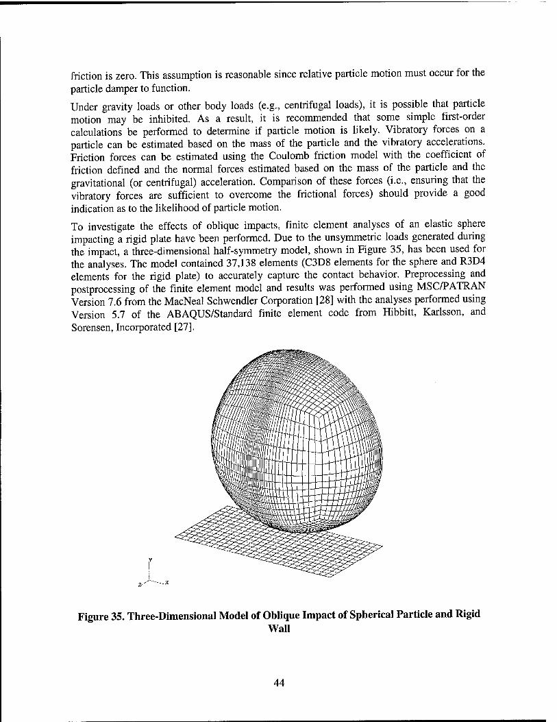
friction is zero. This assumption is reasonable since relative particle motion must occur for the particle damper to function.

Under gravity loads or other body loads (e.g., centrifugal loads), it is possible that particle motion may be inhibited. As a result, it is recommended that some simple first-order calculations be performed to determine if particle motion is likely. Vibratory forces on a particle can be estimated based on the mass of the particle and the vibratory accelerations. Friction forces can be estimated using the Coulomb friction model with the coefficient of friction defined and the normal forces estimated based on the mass of the particle and the gravitational (or centrifugal) acceleration. Comparison of these forces (i.e., ensuring that the vibratory forces are sufficient to overcome the frictional forces) should provide a good indication as to the likelihood of particle motion.

To investigate the effects of oblique impacts, finite element analyses of an elastic sphere impacting a rigid plate have been performed. Due to the unsymmetric loads generated during the impact, a three-dimensional half-symmetry model, shown in Figure 35, has been used for the analyses. The model contained 37,138 elements (C3D8 elements for the sphere and R3D4 elements for the rigid plate) to accurately capture the contact behavior. Preprocessing and postprocessing of the finite element model and results was performed using MSC/PATRAN Version 7.6 from the MacNeal Schwendler Corporation [28] with the analyses performed using Version 5.7 of the ABAQUS/Standard finite element code from Hibbitt, Karlsson, and Sorensen, Incorporated [27].

Figure 35. Three-Dimensional Model of Oblique Impact of Spherical Particle and Rigid Wall

44

Initial analyses investigated an elastic sphere of radius 0.0625 inch impacting the rigid wall at a velocity of 62.832 in/s at an angle of 45° relative to the rigid wall. The sphere was given steel properties with an elastic modulus of 30x10^ Ibf/in^ a density of 0.283 lbf/in^ and a Poisson's ratio of 0.33. A coefficient of friction of 0.60 was prescribed. Predicted normal and shear loads resulting due to the oblique impact are shown in Figure 36.

2.00E+01

1.50E+01

1.00E+01

5.00E+00

O.OOE+00

-5.00E+00

—1— ■ 1 1 1

-°-ABAQUS Normal Load

-«-ABAQUS Shear Load for mu=0.6

1 1 1 1

\/\\\

''"A A ^ 'jr:\:y^^,^

—ni

O.OE+00 2.0E-05 4.0E-06 6.0E-06

Time (sec)

8.0E-06 1.0E-05

Figure 36, Predicted Normal and Shear Loads Resulting from Oblique Impact

Figure 37, Figure 38, and Figure 39 show predicted normal and shear loads versus time from ABAQUS and as predicted using the Coulomb friction model for impacts at angles of incidence of 60°, 45°, and 15°, respectively (where the angle of incidence is the angle between the particle velocity vector and the direction perpendicular to the rigid wall). The normal forces were calculated based on Hertz's theory and, as previously discussed, compare well with the results from ABAQUS. As shown in the figures, the Coulomb friction model generally predicts reasonably accurate shear forces for impacts at higher angles of incidence (more glancing). However, at lower angles of incidence (more normal) the Coulomb friction model can significantly overpredict the shear forces. In addition, the shape of the shear force curve from ABAQUS is different than that predicted using the Coulomb friction model. In the ABAQUS solution, the shear force peaks prior to the peak of the normal force. With the Coulomb friction model, the shear and normal forces peak at the same time. The shear force also undergoes a reversal in the ABAQUS solution, whereas the normal force completes a half cycle only [23].

45

2.50E+01

2.00E+01

1.50E+01

2 1.00E+01

5.00E+00

O.OOE+00

-5.00E+00

1 1

-o-ABAQUS Normal Load

"""Hertz Normal Load

-^ABACUS Shear Load .__ r

1 1

r

r

^=-f-= ̂ ̂^ -i

1—CD if/g^c^co-^^y- p

O.OE+OO 2.0E-06 4.0E-06 6.0E-06

Time (sec)

8.0E-06 1.0E-05

Figure 37. Predicted Normal and Shear Loads Using Coulomb Friction for 60° Impact

2.50E+01

2.00E+01 ■-

1.50E+01

o 1.00E+01

5.00E+00

O.OOE+00

-5.00E+00

O.OE+OO 2.0E-06 4.0E-06 6.0E-06

Time (sec)

8.0E-06 1.0E-05


46

2.50E+01 - 1 ■ 1 1 1 1

\ ./^ _L.. 1

---

-o-ABAQUS Normal Load

^—Hertz Normal Load

-»-ABAQUS Shear Load

""^Coulomb Friction

2.00E+01 ■

1 rj 1 \

1.50E+01 ■

n

r if^

_3 1.00E+01 -

1 5.00E+00 ■

Jp X '

T " T ^ ^ d:: O.OOE+00 1 WwWXCsn^ j 1 1 1 1 1 1

T

O.OE+OO 2.0E-06 4.0E-06 6.0E-06

Time (sec)

8.0E-06 1.0E-05


Investigating the shear forces further, one finds that the shear force-displacement relations are extremely complex. For example, the force-displacement relations can independently display nonlinear response, path dependence, and dissipation due to slip, even v^'hen the spheres are linearly elastic and the relative displacements are small. Mindlin and Deresiewicz [29] established a detailed set of equations depending on whether the normal and shear forces are increasing, decreasing, or remaining constant. Their theory is limited to so-called simple loading histories and includes 11 loading cases. Simple loading histories begin with an equilibrium position for which the distribution of traction is equivalent to a state of constant normal force and varying shear force, and advance to the desired state through a sequence of equilibrium positions. The final distribution of traction is equivalent to another state of constant normal force and varying shear force. Due to the complexity of these relations, efficient implementation within the particle dynamics method is not possible. As a result, various simplified contact force-displacement relations have been proposed.

Walton and Braun [30] proposed an incremental equation, based on a tangential stiffness coefficient and the incremental tangential displacement, to approximate the Mindlin and Deresiewicz contact mechanics theory. For cases where the normal force remains constant, this method generates results in general agreement with those from Mindlin and Deresiewicz. However, for particle damping simulations, and the majority of particle dynamics simulations, both the normal and shear forces are changing during the impact event.

Vu-Quoc and Zhang [31-33] have proposed an improved version of the model by Walton and Braun which incorporates selected cases of varying normal and shear forces from Mindlin and Deresiewicz, and a correction for the rolling effect. Although these relations are simpler than

47

those of Mindlin and Deresiewicz, considerable computational resources still are required. As an example, Vu-Quoc and Zhang [33] performed simulations of 400 soybeans falling through a chute, which required approximately 19 CPU hours for 1 second of simulated time. As discussed in the following Experimental Validation and Sample Application sections, particle damper simulations may require solutions for tens of seconds. The computational resource requirements make implementation of the Vu-Quoc and Zhang relations impractical.

A simpler, more efficient method which can reasonably account for the tangential force- displacement relations is required. Maw, Barber, and Fawcett [34-35] proposed a solution for the oblique impact of an elastic sphere where the contact area is broken into a series of concentric circles. In each of these separate regions, sticking or slipping can occur. At the beginning of each step in the solution, each of the regions is assumed to either stick or slip. The appropriate equations are solved and the solution is tested to see if the initial assumptions were correct. In stick regions, the tangential force must not exceed the limiting force given by the Coulomb friction model. In slip regions, the incremental displacement must be in the correct sense for the assumed frictional traction. If either of these tests fails in any region, the initial assumptions are revised and a new solution is obtained. At each contact increment, a solution must be found for each of the different regions (which may be on the order of 20); each solution must be checked to verify that the initial assumptions for that particular region are correct; and, as necessary, new solutions must be found for those regions in which the initial assumptions were violated. As a result, this method is relatively inefficient.

Maw, Barber, and Fawcett extended their work by calculating the shear forces for various oblique impact conditions and found that the variation in the shear force during the impact could be found based on two nondimensional parameters. These efforts are outlined in Johnson's Contact Mechanics [23] and have the advantage of using the non-dimensional parameters to turn the computationally intensive procedure into one where results can be found to fall on a specific curve. The peak shear forces predicted using the Maw, Barber, and Fawcett model compare relatively well with the peak shear forces from ABAQUS and the model captures the basic form of the curve including the reversal. The peak shear force predicted using the Maw, Barber, and Fawcett model occurs earlier in the impact event than that predicted by ABAQUS and, particularly for intermediate angles of incidence, a much larger negative shear force is predicted during the reversal.

All of the shear force-displacement models discussed above suffer from the same general flaw that, in general, it is not possible to know a priori whether a contact will be enduring or not. The relations discussed above are based on a single discrete impact, and may not accurately predict the shear forces for enduring contacts or for particles experiencing multiple contacts at once. In the particle damper model, it is more critical to accurately represent the enduring contacts since these contacts generally last for a longer time and can have a more significant effect on the damping. As a result, shear force-displacement relations for oblique impacts have been implemented in the particle damping model using the same Coulomb friction model used for enduring contacts. Future enhancements to the particle damper model may include a more accurate representation of the shear forces generated during oblique impacts.

7.3 Implementation The background of the particle damper simulation code is based on X3D, an explicit finite element code typically used for impact analyses [36]. The code contains various contact

48

algorithms and bookkeeping routines and provides an appropriate framework for simulating particle damping through the use of the particle dynamics method. Particle-particle and particle-cavity contacts are resolved using the force-displacement relations discussed in the preceding paragraphs. Separate contact detection/resolution routines are used for particle- particle and particle-cavity contacts.

Particle-cavity contact detection is performed using a modified version of the master-slave algorithm from X3D. As shown in Figure 40, three-node triangular master surfaces are used to define the cavity with the particles existing as slave nodes. At each time step, geometry checks are performed to resolve any contact between the slave nodes (particles) and the master surfaces (cavity). Since the cavity walls are assumed to be flat, the nodes used for the master surface lie in a plane. An orthogonal local coordinate system is constructed with two directions, Xi and X2, as shown in the figure, in the plane of the master surface and the third direction, X3, perpendicular to the contact surface. The distance in the X3 (normal) direction between the particle center and the master surface is calculated. Contact is detected if this distance is less than the particle radius. The particle translational velocity, Vp, is broken into components in the local coordinate system. Similarly, the master node velocities (v^i, Vm2, and Vms) are broken into translation components in the local coordinate system. Any particle rotation, (Op, is broken into rotations about the in-plane (xi and X2) axes. Spin (i.e., rotation about the X3 axis) is neglected. The relative normal velocity is calculated based on the X3 component of the particle velocity and X3 contributions from each of the master nodes. Relative tangential velocities are calculated based on the in-plane velocity components of the particle and the in-plane velocity contributions from each of the master nodes, as well as the particle rotations about the in-plane axes. A slight error is introduced as the velocity contributions from the particle rotation about the in-plane axes are based on undeformed particle radii rather than the instantaneous radii.

Figure 40. Particle-Cavity Contact Detection and Resolution

Particle-particle contact detection is performed by tracking the nodes at the center of the particles as shown in Figure 41. The distance between each set of particle centers is calculated. Contact is detected if this distance is less than twice the particle radius. The relative velocity at the point of contact is calculated in global coordinates based on the translations (Vpi and Vp2) and rotations (cOpi and tOp2) of the contacting particles. As with the particle-cavity contacts, a slight error is introduced as the velocity contributions from the particle rotations are based on

49

undeformed particle radii rather than the instantaneous radii. A unit normal vector in the direction connecting the particle centers is calculated in global coordinates. The relative normal velocity can be calculated by taking the dot product of the relative velocity vector at the point of contact with the unit normal vector. The relative tangential velocity then can be calculated by subtracting the relative normal velocity from the overall relative velocity.

Figure 41. Particle-Particle Contact Detection and Resolution

The force-displacement relations used to resolve both particle-cavity and particle-particle contacts are formulated in incremental form. As a result, whenever contact is detected, it is necessary to determine whether it is a new or existing contact condition. Checks are made to determine if the contact condition existed at the previous time step and appropriate information from the previous time step, which is required to calculate the forces at the current time step, is stored. A constant time step has been used throughout the simulations.

7A Summary of Model Assumptions and Limitations The following is a summary of the primary assumptions and limitations of the particle damper model:

• All particles assumed to be identical; particles are assumed to be spherical in shape with a given radius and material properties.

• Particles can be given elastic or viscoelastic material properties; viscoelastic material properties are given as a three-parameter Maxwell model.

• Cavity walls are assumed to be flat and rigid.

• A single coefficient of friction is used for particle-particle and particle-cavity contact.

• The kinetic coefficient of friction is given; i.e., it is assumed that particle motion occurs or that the static coefficient of friction is zero.

• Normal force-displacement relations are based on a modified form of Lee & Radok's relation (where the elastic modulus is replaced with the relaxation modulus) with the force set to zero when a negative force is predicted.

• For elastic properties, the normal force-displacement relation reverts to an incremental form of Hertz's relation.

50

• For viscoelastic properties, an incremental form of the force-displacement relation is used which incorporates relaxation behavior of the viscoelastic material.

• Shear force-displacement relations are based on Amonton's law of sliding friction, or Coulomb friction.

• The shear force magnitude is based solely on the magnitude of the normal force and the coefficient of friction.

• The direction of the shear force opposes the relative tangential velocity between the contacting surfaces; relative tangential velocities can result from oblique impacts or due to rotation of the particles.

7.5 Particle Damper Design IVIettiodoiogy As discussed in the preceding paragraphs, an analytical particle damper model has been developed which captures the complex interactions of the loss mechanisms in a particle damper. This simulation technique has been incorporated into a comprehensive particle damper design methodology which allows particle damping to be implemented without extensive trial- and-error testing. Critical steps in the design process include the following:

1. Determine characteristics of undamped system.

2. Determine appropriateness of particle dampers.

3. Select particle damper configuration.

4. Determine characteristics of undamped system with adjusted mass.

5. Evaluate damper effectiveness using particle damper simulation technique.

6. As necessary, repeat steps 3-6.

7. Verify chosen design experimentally.

The initial step in the particle damper design is to establish the characteristics of the system to be damped. Key characteristics include the resonant frequencies of the structure and the vibratory displacements of the system. These characteristics will typically be determined through a combination of experimental testing and finite element analysis. Additional concerns include the environmental conditions under which the damper must operate (e.g., at cryogenic or elevated temperatures). Geometric constraints, which may limit the location and/or size of the particle damper cavity, also must be considered.

The second step in the design methodology is to determine if particle dampers are appropriate. Particle damping is typically most effective in damping well-separated, resonant modes of a structure with relatively large vibratory displacements (which usually occur at lower order modes). However, particle dampers may provide some damping under extreme conditions where other options are not feasible.

The next step in the methodology is to select a specific particle damping configuration. To aid in the selection of an effective particle damper configuration, a list of basic "rules-of-thumb" have been established. These rules are based on measured results from experimental testing, predicted results from analytical modeling, and published results from other researchers [37- 38]. Key design guidelines include the following:

51

• Total particle mass appears to have a fairly significant effect on damping for both single particle and multiple-particle dampers. Increasing the mass tends to increase the damping. Conversely, decreasing the mass tends to reduce damping. As might be expected, changes in the total particle mass can lead to a fairly significant shift in the frequency of peak response.

• Increases in the coefficient of friction or viscoelasticity of the particles tend to increase the damping for single-particle dampers. For multiple-particle dampers, very little effect, or perhaps even a slight adverse effect, on the damping is observed.

• For single-particle dampers, orienting the dampers such that gravity is in the direction of the vibratory motion tends to reduce the damping. The orientation of gravity appears to have much less effect on dampers with multiple particles.

• Both single- and multiple-particle dampers appear to exhibit maximum damping at an optimum excitation level. Lesser damping is observed at excitations above and below this specific level. This relationship is closely linked to the interior dimensions of the cavity, particularly the length of the cavity in the direction of the vibratory motion.

• Single-particle dampers appear to be more sensitive to changes in the various particle damper parameters. This result illustrates a potential advantage of multiple-particle dampers in that precise tuning of the damper parameters may be less critical.

• At times, both the single- and multiple-particle dampers may cause random, somewhat chaotic, behavior of the damped system (e.g., the system may exhibit several local response peaks instead of a single resonant peak). This behavior occurs more commonly in systems where the particle damper is contributing significant damping and may result due to slight mistuning of the damper parameters.

Once a specific particle damper configuration has been selected, the characteristics of the undamped system again must be determined to incorporate the effects of any added (or reduced) mass due to the particle damper cavity. Often it is not practical to simulate the entire physical system with the particle damper attached. Therefore, the specific mode of the system to be damped is modeled as a SDOF, sinusoidally excited, mass-spring-damper system. It is necessary to determine the generalized mass, spring stiffness, viscous damping coefficient, and drive force from the undamped physical system to develop the analytical SDOF model. Even for cases where the entire structure is to be modeled, it is necessary to perform this step to ensure that the added cavity mass does not drastically affect the natural frequencies or modes of interest.

Once a particle damper configuration has been selected and the characteristics of the undamped system with adjusted mass have been determined, the analytical model can be used to evaluate the damping effectiveness. Effectiveness can be evaluated by comparing vibratory displacements for the undamped and damped cases. Similarly, the relative effectiveness of particle damper designs can be determined by comparing predicted displacements. Specific details on using the analytical particle damper model for specific applications are given in Sections 8 and 9. In these sections, predicted results from analytical particle damper models are compared with experimental test results for a cantilevered beam and an aluminum box structure.

52

Based on the results of the particle damper simulation, it may be determined that the chosen damper configuration does not provide sufficient damping. Even if the damping is sufficient, it may be desirable to investigate alternative designs to determine if similar damping levels can be achieved with lower added mass or using more readily available materials. The guidelines given above provide some guidance in identifying new damper configurations. If the damper cavity configurations remain the same, new simulations can be performed using the previously determined system parameters. Otherwise, the characteristics of the undamped system with the new cavity configuration must be determined. Several design cycles may be necessary to define an effective particle damper configuration.

Lastly, once an acceptable particle damper configuration has been established, the damper should be fabricated and applied to the structure. Experimental measurements should be taken to verify the effectiveness of the particle damper and to ensure that there are no adverse effects on other modes of the system or clearance issues.

53

8 Correlation with Experimental Beam Tests Experimental testing and analytical simulations were performed to validate the model discussed in the previous section. A cantilevered beam was tested undamped and with various impact dampers and particle dampers attached. The test data was then compared to analytical prediction.

8.1 Experimental Testing The first flexural mode of a cantilevered aluminum beam was used for the experimental testing. The behavior of a vibrating beam is well understood and permits the use of simple hand calculations or finite element models to evaluate the effect of various modifications, such as the shift in natural frequency due to added mass. This system also can be used to roughly approximate a single degree-of-freedom system. The testing was performed using an aluminum beam 12.0 inches in length, 1.50 inches wide, and 0.175 inch thick, as shown in Figure 42. The beam was rigidly fixed at the root and had a first flexural mode of slightly less than 40 hertz.

Figure 42, Aluminum Beam Used for Correlation Testing

Experimental testing was performed on the undamped beam, on beams with added mass, and on beams damped with impact and particle dampers containing stainless steel spheres. The impact and particle damper cavities were constructed from square acrylic tubing with an outer edge length of 0.500 inch and a wall thickness of approximately 0.065 inch. Aluminum end caps were epoxied to the tubing to enclose the cavities. Stainless steel spheres of various radii were used for the particles.

8.2 Analytical Simulation Analytically, the beam used for the experimental testing is modeled as a simple mass-spring- dashpot system, as shown in Figure 43. The beam is modeled using a lumped mass (at the master cavity node) attached to a damped spring-to-ground element. The equivalent mass, spring stiffness, and viscous damping coefficient are chosen to simulate the undamped beam.

54

Stiffness and damping defined to simulate aluminum beam system

r^N\fW\l\N\^]

Master cavity node used to track position of cavity; effective system mass

('-, lumped at this node Q

Cavity created using contact surfaces defined by nodes linked to master cavity node

Node at center of '--' particle determines position

Figure 43. X3D Model Used to Simulate Particle Dampers

The cantilevered aluminum beam used for the experimental testing is 12.0 inches in length, 1.50 inches wide, and 0.175 inch thick, and has an elastic modulus of 10.0x10^ psi and a density of 0.100 Ibf/in^ (2.59x10""^ Ibf-s^/in^). The mass of the beam can be calculated as follows:

m = pV = (0.100X12.0X1.50X0.175)= 0.315 Ibf = 8.15851x10" Ibf-s'

m (34)

The equivalent mass, m,^, for a cantilever beam of mass, m, carrying an end mass, M, is given

as follows [39]:

m„„ =M + 0.23m

For the undamped beam, the equivalent mass can be found as follows:

m,q = 0.23m = (0.23X8.15851x10-")= 1.87646x10"'

The stiffness of the beam, k, is calculated as follows

k

m

_ 3EI _ (3)(l0.0xl0^)(6.9922xl0")_^^^3p^^^,i Ibf

1^ (12^

where the moment of inertia, I, is calculated as follows:

(35)

(36)

(37) m

bh^ ^ (l.50X0.175y _ -4-4 6.69922x10"'in 12 12

The natural frequency of the beam, Wbeam or f^eam. is calculated as follows:

(38)

55

CO beam m, eq

: 248.961— or f, s beam

= .9^beam ^ 39 g23 Hz 271

(39)

The measured natural frequency of the undamped beam is 39.37 Hz, or 247.369 rad/s. The analytical simulations use an adjusted stiffness of 1.14823x10' Ibf/in such that the natural frequency is identical to the measured frequency of 39.37 Hz.

The beam system is excited by a prescribed sinusoidal force applied at the master cavity node. Initial estimates for the analytical drive force are made based on the tip force equivalent to the measured force input near the root of the beam. Initial damping estimates are made based on the measured loss factor from experimental testing. The excitation force and damping are adjusted such that the predicted response of the undamped beam from the analytical simulations matches the undamped response measured experimentally. Thus, the analytical model is tuned for the undamped response. Subsequent damped analyses utilize the tuned model parameters. The drive force, equivalent mass, spring stiffness, and viscous damping coefficient used to model the undamped beam in X3D for an excitation of 200 mV RMS to the shaker are given in Table 4.

Table 4. Parameters Used to Simulate Undamped Beam for X3D Analyses

Parameter Value

Drive force 4.84040x10"^ Ibf

Equivalent mass 1.87646x10-^ Ibf-s^/in

Viscous damping coefficient 3.08293xlO"Mbf-s/in

Spring stiffness 1.14823x10' Ibf/in

For damped simulations, the cavity is modeled using contact surfaces defined by nodes which are linked to the master cavity node. Particles are tracked using a node at the center of each particle. The particles are initially given a random distribution within the cavity and include a gravity load which ensures that the particles pack on the bottom of the cavity. The mass of the particles is included based on the prescribed number of particles and the radius and density of each particle. Any additional mass due to the cavity must be added to the equivalent mass of the undamped beam. Material properties are given for the particles to incorporate the elastic or viscoelastic impact behavior. A coefficient of friction also is given for the particles to account for friction interactions between the individual particles or between the particles and the cavity walls.

A sample input deck for the aluminum beam with a particle damper cavity with interior dimensions of 0.372 inch wide, 0.372 inch high, and 0.263 inch long, containing 64 0.03125- inch radius particles is given in Appendix A. The basic geometry of the system is defined using the NODE COORDINATES, ELEMENTS, and CONTACT cards. The position of various nodes within the model are defined using the NODE COORDINATES card. These nodes are required to define the cavity geometry and master cavity node, as well as to track the particle

56

centers. The damped spring-to-ground element is created using the ELEMENTS card and provides a link between the master cavity node and a fixed point (ground). The spring stiffness and viscous damping coefficient for this element are defined on the MAT ID card. The CONTACT card is used to define 12 triangular master contact surfaces, which define the cavity geometry, along with slave nodes corresponding to the center of each particle. Properties for the particles are defined on the PDMP card. Basic input parameters for the PDMP card are given in Appendix B (the PDMP card has been created specifically for particle damper simulations and is not included in the basic X3D user's manual). The BODY card is used to simulate gravity such that the particles tend to fall to the bottom of the cavity. The equivalent mass of the system is lumped at the master cavity node using the MASS card. Note that an equivalent mass of 2.04213x10""^ Ibf-s^/in is used which includes the mass of the aluminum beam plus the additional mass of the damper cavity (but not the particles). The RBEL card links the cavity nodes to the master cavity node and is used to ensure that the entire cavity moves as a single unit. The BOUNDARY CONDITIONS card ensures that the cavity only moves in the direction of the applied force. The TITLE card allows a descriptive title to be assigned to the analysis. The PARAMETERS card sets parameters relating to the total simulated time, the timestep, the total number of timesteps, and the frequency at which results are output to the trace file. For these analyses, simulations are run for 15 seconds using a timestep of 0.5 microsecond. Results are output to the trace file every millisecond. Lastly, the TRACE card is used to define those nodes for which output to the trace file is requested. Typically, results for the master cavity node are output along with results for each of the particles. Further details on the various options available for each of these cards (with the exception of the PDMP card) are given in the X3D user's manual.

The excitation force used for a simulation is defined in the USRFRC subroutine which must be included in the compilation of the X3D code. The X3D code contains a skeleton version of the USRFRC routine. A sample USRFRC subroutine modified for particle damper simulations is given in Appendix C. This sample routine imposes a force of 4.84040x10"^ Ibf at a frequency of 37.21 Hz, or 233.797 rad/s. The force is applied at node 25, the master cavity node. To perform simulations at other drive frequencies or excitation levels, or with other master cavity nodes, this subroutine must be modified and a new version of X3D compiled. The master cavity node also is currently hard-coded on two lines (which set the variable NODEM) in the PDFORC routine. These lines also must be modified to change the master cavity node.

8.3 Results Figure 44 shows selected frames from early in the 64 particle simulation as discussed above. Note that the particles are initially given a random distribution within the cavity (as shown in the upper left frame at a time of 0.0 s) but quickly pack on the bottom of the cavity due to gravity (as shown in the lower right frame at a time of 0.10 s). The frames shown below have been created using a MATLAB routine which processes the data output to the trace file. The frames can be animated to observe the cavity and particle motion.

57

Particle Dampor Simulalion

Simulated Time (sec): 0-OOOOOe+OOO

Particle Damper Simulation

Simulated TlmQ (sec): 2.00000e-002

0.1 0.2 0.3 0.4 0.5 0.1 0.2 0.3 0.4 0.5


Sim Jaled Time (sec): 4.0C00Oe-O02


Simulated Tims (sec): 6,000009-002

0.1 0.2 0,3 04 0.5 0.1 0,2 0.3 0-4 0.5

Particle Damper Simulalion

Simulated Time (sec): 8.00000e-002


SimJaled Time (sec): I.OOOOOe-001

0.1 0.2 0.3 0-4 0,5 0.1 0.2 0.3 0.4 0.5

Figure 44. Selected Frames from Particle Damper Simulation

Various simulations have been performed corresponding to cases which have been tested experimentally. Measurements have been made for the undamped beam, the beam with an added mass equal to the mass of the dampers, and for various particle damper configurations (of the same total particle mass) containing 1 0.250-inch diameter particle, 64 0.0625-inch diameter particles, and 512 0.03125-inch diameter particles. Figure 45 shows experimental and analytical beam tip displacements at various frequencies for the undamped, added mass, and single particle configurations under a force equivalent to a 200 mV RMS excitation signal to the shaker. Figure 46 shows results for the various damped cases under a force equivalent to a 200 mV RMS excitation signal to the shaker. Similar results corresponding to a 400 mV RMS excitation signal to the shaker are shown in Figure 47 and Figure 48.

58

For all of the damper analyses, the particles are given viscoelastic material properties with EQ

equal to 27.5x10^ psi, Ei equal to 5.0x10^ psi, and Xi equal to 2.0x10"^ second (corresponding to a maximum equivalent loss factor of 0.083). A coefficient of friction of 0.30 has been used in the analyses. For some of the experimental results, two sets of data are given for the same configuration. In each case, the first set of results corresponds to data taken with the excitation frequency increasing during testing and the second set with the excitation frequency decreasing. An interesting result is observed in the experimental data for the damper with 512 particles. Under 200 mV RMS excitation, very little attenuation is seen. However, under 400 mV RMS excitation, considerable attenuation is observed once the displacements reach a certain level (whether the excitation frequency is increasing or decreasing). During experimental testing it has been observed that the small particles in this damper tend to clump together, and it is believed that there may be cohesive forces between the particles due to static electric charges or oil on the particles which influence the results.

In general, the particle damper simulation code predicts the correct trends. For example, the model predicts little attenuation for the single particle dampers, but considerably more attenuation for multiple-particle dampers containing 64 and 512 particles. The model also captures the experimental trend of optimum damping at a specific number of particles with lesser attenuation when either a smaller or greater number of particles is used. This trend is evident in the increased attenuation observed when the number of particles is increased from a single particle to 64 particles; and the decreased attenuation observed when the number of particles is further increased to 512 particles. The model does tend to overpredict the attenuation, particularly for multiple-particle dampers.

8.00E-02

7.00E-02

42.00

Figure 45. Beam Tip Displacements with 200 mV RMS Excitation Force

59

8.00E-02

7.00E-02

6.00E-02

5.00E-02

4.00E-02

I- E S 3.00E-02 m

2.00E-02

1.00E-02

O.OOE+00

1 1 Da

■•♦-■(1)0.250Steel(ss001a) shed - Experimental Solid - Analytical

• • * • • (64) 0.0625 Steel (ss003a)

/

1 COF=0.30

• ^ ■' (64) 0.0625 Steel (ss004a)

•-- "-(64) 0.0625 Steel (hcomp17) d <»

■ ■• - ■ (512) 0.03125 Steel (ss007a)

—Cl—(512) 0.03125 Steel (icompi?) VA / 'M

/.iMw. 4#n--i-$:;~.-,

^^^^^-'^"■^

I..i'"-''''''' " ~->i -■-.-„„„ •■

35.00 35.50 36.00 36 50 37.00 37.50

Frequency (Hz)

38.00 38.50 39.00

Figure 46. Damped Tip Displacements with 200 mV RMS Excitation Force

1.60E

O.OOE+00

Figure 47. Beam tip displacements witli 400 mV RMS excitation force

60

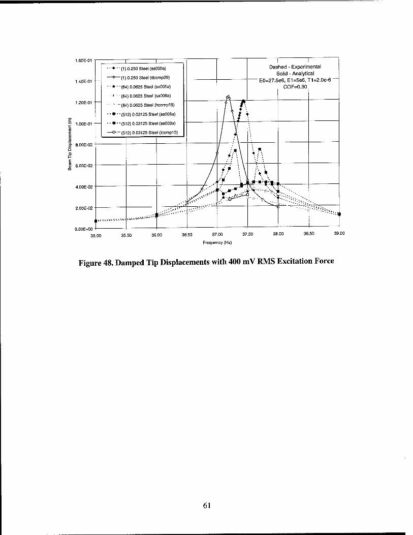
1.60E-01

1.40E-01

1.20E-01

1.00E-01

S- 8.00E-02

S 6.00E-02

4.00E-02

2.00E-02

O.OOE+00

■-(1)0.250 Steel (ss002a)

- (1) 0.250 Steel (dcomp29)

• • (64) 0.0625 Steel (ssOOSa)

■ • (64) 0.0625 Steel (ss006a)

(64) 0.0625 Steel (hcomp19)

• • (512) 0.03125 Steel (ssOOBa)

■ ■ (512) 0.03125 Steel {ss009a)

— (512) 0.03125 Steel (icomplQ)

35.00 35.50 36.00 36.50 37.00 37.50

Frequency (Hz)

38.00 38.50 39.00

Figure 48. Damped Tip Displacements with 400 mV RMS Excitation Force

61

9 Correlation with Experimental Chassis Tests Additional experimental testing and analytical simulations have been performed on an aluminum chassis. The basic experimental test setup, analytical modeling details, and correlation of experimental results with analytical predictions are discussed in the following paragraphs.

9.1 Experimental Testing The aluminum chassis used for this testing, along with corresponding test hardware, is shown in Figure 49. The structure and related hardware are from a previous effort and provide a suitable article for particle damping. The chassis is basically an aluminum box with dimensions of 17.0 inches in length, 8.0 inches in width, and 3.0 inches in depth. The box is constructed from aluminum sheet with a nominal thickness of 0.049 inch. The box is supported by a relatively stiff aluminum structure as shown in the figure. The entire lower edge of the box is fixed.

1 '

I, . If /

Figure 49, Aluminum Chassis Structure and Test Hardware

The particle dampers are focused on attenuating the fundamental mode of the structure. For this mode, most of the motion is seen in the upper surface of the box with the displacements following roughly half of a sinusoidal cycle in both the width and length directions. The deformed shape of the first fundamental mode, as predicted by finite element analysis, is shown in Figure 50.

62

MSC/PATRANVeiil!jn9.02S-Jin-01 W:09:4] Deform: Def»u!r.S!epl.Model.Pruhl41,S3 Hz. Defcrm8t]Dn.IJlipl*Mm KM. {NON-LAYERED}

Figure 50. Fundamental Mode of Box Structure

Similar to the beam testing, the box is excited through a stinger which is centered across the 8.0 inch width of the panel and located 3.425 inches above the bottom of the panel. A force gage is located between the stinger and the box to record the actual force input into the structure. A sinusoidal signal is passed to the shaker, with the input voltage controlled to maintain a specific excitation force. An accelerometer is positioned at the center of the panel, on the inner surface of the box, to record accelerations.

The damper is placed at the center of the panel, on the outer surface of the box, where the largest displacements are seen for this mode (and are relatively large compared to the maximum displacements of other higher order modes). The damper cavity is fabricated from square brass tubing with an outside edge length of 0.500 inch and a wall thickness of 0.028 inch, yielding an interior edge length of 0.444 inch. End caps constructed from a 0.028-inch- thick brass sheet are epoxied to the ends of the tubing to create the cavities. The cavities have an interior length of 0.350 inch. Initial studies have been performed using particle dampers containing 128 spherical stainless steel particles with a diameter of 0.0625 inch.

9.2 Analytical Simulation Analytical particle damper simulations have been performed using both a SDOF model and a multiple degree-of-freedom (MDOF) model. The SDOF model is similar to the model used for the beam simulations. The aluminum box structure is modeled as a simple mass-spring-dashpot system, with the analytical model tuned to match the response of the undamped structure. The drive force, equivalent mass, spring stiffness, and viscous damping coefficient used to model the undamped box structure in X3D for a 0.1 Ibf RMS excitation are given in Table 5.

Table 5. Parameters used to simulate undamped box structure for X3D analyses

Parameter Value

Drive force 5.65771x10"^ Ibf

63

Equivalent mass

Viscous damping coefficient

Spring stiffness

3.54282x10"'* Ibf-s^/in

-3 3.55000x10"^ Ibf-s/in

1.95442xlOMbf/in

Additional analytical simulations have been performed using a MDOF model. For these simulations, the entire box structure is modeled. A relatively coarse mesh is used since only the fundamental mode is of concern and to reduce the likelihood of higher frequency noise in the solution. The model used for these analyses is shown in Figure 51. For these simulations, the force from the stinger is applied at the actual location used for the experimental testing, rather than at the master cavity node. The node at the center of the panel is used as the master cavity node and the predicted vibratory accelerations are recorded at this node. The cavity and particles are modeled and tracked as in the SDOF simulations.

Figure 51. Model Used for MDOF Simulations

9.3 Results Experimental testing and analytical simulations have been performed at various excitation levels and across a range of frequencies. The response of the undamped chassis structure, and the chassis structure with particle dampers containing 128 particles, has been investigated. Results are presented as accelerance (in this case, the ratio of the vibratory accelerations at the center of the panel to the input force at the shaker location) versus frequency. Figure 52 compares results from the experimental testing and simulations using the SDOF model. Some interesting results are seen in the experimental data. At the 0.1 Ibf RMS excitation level, the peak response of the damped chassis structure has approximately the same magnitude as the undamped structure, but occurs at a slightly higher frequency. As the excitation level is increased up to 0.5 Ibf RMS, the peak response is attenuated considerably with the frequency of

64

the peak increasing with increasing excitation. Above 0.5 Ibf RMS excitation the damping decreases, but the frequency of the peak continues to increase. It is believed that this behavior results due to a combination of various effects, including changes in damping and effective added mass. Such behavior is not seen in the analytical results. The analyses predict increasing damping with increasing excitation, with the frequency of the peak response decreasing with increasing excitation.

250- 'lilt

—1 1 1 1 1 1 i I

1 1 1 1 1

-- 200-

b 150-

—o—0.1 Ibf RMS excitation - experiment

■ - ♦ ■ -0.1 Ibf RMS excitation - simulation

—*—0.25 Ibf RMS excitation - experiment

• • ♦ ■ -0.25 Ibf RMS excitation - simulation

—'^—0.5 Ibf RMS excitation - experiment

■ - • ■ ■ 0.5 Ibf RMS excitation - simulation

1 1

■ ■ * • ■ 1.0 Ibf RMS excitation - simulation

i i /JV'M*--. vi 1 1 1 1 1 1 ' 1 III'

g 100-

r"'i'""""i^p^^j i 1 1 50-

0 J

"^^^ \ ^^^^M^ ,

110 112 114 116 118 120 122

Frequency (Hertz)

124 128

Figure 52. Comparison of Experimental Measurements and SDOF Analysis Results

Analyses with the MDOF model have been performed to determine if the discrepancy between the experimental and SDOF model results is due to the inability of the SDOF model to accurately capture the dynamics of the chassis structure. Figure 53 compares results from the experimental testing and simulations using the MDOF model. Results from the MDOF model are similar to those from the SDOF model. Although the undamped model could be more accurately tuned to match the experimental response of the undamped structure, it is unlikely that this would have much of an effect on the results. Changes in the coefficient of friction and viscoelastic properties do not appear to have a large effect on the overall peak response. As a result, it is thought that the momentum transfer may have a critical effect on the damping. Reductions in the forces transferred to the structure reduce the damping and correlate better with the experimental results. It is possible that compliance of the cavity walls, which are currently assumed to be rigid, may contribute to the discrepancy. It is recommended that future efforts focus on ensuring that appropriate forces are applied during impacts between the particles and the cavity walls.

65

250

200--

150

S 100--

50--

^ ^ 1 1

1 1 1 I <

—1 1 1 1

'III

1 1 1 1 -- —0—0.1 Ibf RMS excitation - experiment

■■■♦■• -0.1 Ibf RMS excitation - simulation

—«—0.25 Ibf RMS excitation - experiment

■ - ♦ "0.25 Ibf RMS excitation - simulation

—CJ—0.5 Ibf RMS excitation - experiment

• ■ * - '0.5 Ibf RMS excitation - simulation ' ' iim \VU i

ffm 1 1 I 1 1 1 1 1 1 1 1 1 1 1 1 1 1 t 1 1

1 1 1 1

y'''\m^^ \ [ \ "^^f \ ^^m^ 110 112 116 118 120 122

Frequency (Hertz)

124 128 130

Figure 53. Comparison of Experimental Measurements and MDOF Analysis Results

66

10 Proof of Concept Engine hardware for application of the MPED treatment using the design methodology was selected with the aid of Pratt & Whitney. The hardware was a divergent flap backstructure subcomponent for the high speed civil transport. The four-ribbed subcomponent shown in Figure 54 is approximately 12 by 12 by 4 inches high. A two-ribbed structure has been made available to CSA for design and testing of particle dampers. The structures were designed for high temperature capability and acoustic noise reduction. They were made from gamma- titanium to reduce part weight. This material is also brittle and has very low inherent damping. High cycle fatigue is a large problem for these types of structures.

Figure 54. Four-Ribbed Subcomponent at Pratt & Whitney Test Facility

A finite element model of the two-ribbed structure was created. Both ribs were modeled using finite element (FE) and are shown in Figure 55. The first four distinct modes are shown in Figure 56.

67

Figure 55. FE Model of Two-Ribbed Subcomponent

||X,

Figure 56. First Four Distinct Modes

The structure was mounted on a shake table as shown in Figure 57. Data was initially collected for the undamped structure. The frequency response is shown in Figure 58. Random excitation

68

was used with a 1,000-Hz bandwidth. The first mode is apparent at 177 Hz. The second mode is 240 Hz. The first mode is the mode to damp. Particle damping will have effect on the higher modes, as well.

The first-mode peak displacement of the undamped structure was 3.25e-4 inches. An impact damper with slightly less than 6.5e-4 clearance between the particle and cavity wall should have the most influence on the structure.

Figure 57. Substructure Mounted on the Shaker Table (1 50-Particle Damper Attached)

69

Undamped 20

-20

-40

-60

-100

-120

-140

1 —1 1 1 1 1 1 t 1 1

1 1

rt accehg mid accehg

1 1 1 1 1 1

r r r r r 1 1 1 1

1 1 1 1 1 1 1 1 1 i 1 1 1 1 1 i 1 1

1 1 1

. I 1 ! 1 '

1 1 1 1 1 1 1 1 1 1 1 1 1 1 1 1 1 1 1 1

:/ 1 \ \ 1 ! 1 1

\ [;' \ 1 1

1 V 1 1 1

1 1 1 1

: ;: 1 1 1 :| 1 1 1

V. . ; 1 1 1 V-' 1 1 1

\ 1 1 1 xHki 1 1 1 1 __ L ''\ L vuCuf

'~"~\""\""\ i 1 rv! ; y' 50 100 150 200 250 300 350 400 450 500

Frequency (Hz)

Figure 58. FRF for Undamped Structure

The FE model was used to calculate the moments of inertia. As a representative aircraft structure, weight was considered important. A simulation was run for a MPID containing 50 0.0625-inch-diameter stainless steel 302 particles. The cavity was brass having a 0.25-inch inner-length cubic interior with 0.027-inch wall thickness. A comparison of the simulated results with the undamped structure is shown in Figure 59. This run showed that the MPID would give good results, but it over-predicted the damping. The measured FRF for the single cavity with 50 particles is shown in Figure 60.

70

20

-20

q -40

-60

-100 100

Measured Undamped Stmcture versus Simulated 50 0.0625-inch Particies

'1' I

■ -J-U

150 200 Frequency (Hz)

— undamped 50 particles

I \ I \

250

Figure 59. Simulation Response for 50 Particles in Single Cavity

Single 50-particie damper, 2.5V max ioad

20

-20

S -40

-80

-100

1 1 i

rt accel:g mid accei:g

undamped rt accei:g - - undamped mid accel:g

- r 1 I 1

1 i i

=.

/ ■ 1

Jl /■' ' /' /

/'''

V r '■A\

■■\\ >\\ ■\\

1 1 ji

ii -|- _

h

, (1

1 i

100 150 200 250 Frequency (Hz)

Figure 60. Single 50-Particle Damper Measured at Center of Test Article

71

To damp the outer portions of the structure, three 0.25-inch inner-length cubic cavities were constructed and each was filled with 50 stainless steel 302 alloy spherical particles having 0.0625-inch diameter. The cavities were applied at the center and outer "wings," as shown in Figure 61.

Figure 61. Substructure with 3 MPIDs Attached

The FRF for three cavities is shown in Figure 62. As expected, the application of the three cavities affected the both the mode at 177 Hz and the mode at 240 Hz.

The simulation code was used to determine that given the material and geometric constraints of cavity material and size, particle material and size, and structure dynamics, 102 particles would give better damping than 50 particles. Three cavities with 102 0.0625-diameter particles were constructed and applied. The FRF is shown in Figure 63. The increase in the number of particles had a relatively large effect on both the first and second modes. The first mode was reduced by 23 dB. The second mode as measured by the right-hand accelerometer was reduced by 49 dB.

72

Ttiree 50-particle dampers, 2.5V max load

20

-20-

q -40

-60

-80 - -

-100

i'

il ;

rt accei:g — mid accel:g

undamped rt accelig - - undamped mid accel:g

1 '

' f \\ 1 \ ' 1

\ \ 1 _;

Ji^^^'

>HM^'^ 1

100 200 250 Frequency (Hz)

Figure 62.3 50-Particle Dampers

Tliree 102-particie dampers, 2.5V max ioad

S -40

-100 100 150 200

Frequency (Hz)

250

Figure 63.3 102-Particle Dampers

73

11 Commercialization Commercialization is an important part of the SBIR program. CSA applied many of the lessons learned during this SBIR to design a particle damping treatment for a commercial project.

11.1 Introduction A commercial jet-engine manufacturer is developing and integrating an engine that on occasion experiences harmful vibration. This vibration is induced upon stall, a rare event. The level of vibration is unacceptable. Among other things, it causes excessive wear. The vibration is predominantly in a mode with a frequency of about 120 Hz in the test stand configuration. This frequency is expected to increase to roughly 144 Hz in the shipboard application with a different mounting configuration and various test components removed. The engine casing operates at a relatively high temperature, in the range of 600-800 T. Vibration damping using ordinary methods is not feasible at this temperature.

The customer would like to eliminate the vibration problem. One potentially effective approach is to add damping to the system. CSA Engineering is a company that specializes in vibration suppression. CSA has several available methods for damping vibration, although many of these are not applicable at elevated temperature.

CSA proposed to employ alternative methods for reducing the harmful vibration to a point at which its level is acceptable. In this development effort, CSA investigated MPID. CSA designed concepts and produced a prototype for inclusion in upcoming testing.

11.2 Design The following data were supplied by the customer:

1. Typical case vibration is roughly 0.4 inch per second (ips) rms. Max case vibration during stall condition reaches 3.0 ips rms.

2. The entire case weighs 1950 lb. The modal mass participation in the 146 Hz mode of concern is 600 lb. The mode shape is shown in Figure 64.

3. During the stall, the vibration increased from 0.4 ips rms to 3.0 ips rms in slightly less than 5 seconds (Figure 65).

4. The measured damping ratio for the mode is 0.067.

74

TITLE eOlKBll Modal Mass calculation TIME AND DATE 14:58:53 02/067 HARMOmC 1 MODE 9 FREQ. [HZ] KKX UMPXITDDE ¥ TAH

LOAD SET

^--S&=*"

pRt^^"--^ ■-'^-

J^^' -^

^-i;^!^]i:aitt^r:^4!iF^ '' ^*i. 1 Uj I- 4 /

Figure 64. Engine Mode Shape

USZSJS? 13:25:58 13:?5!SJ ISsliSiCrl) JJi?8:0I KJTJSJM 13:26:03 13:25:05 13:25:1)5 13:25:6f

VLfCt, (1P3-BM3) X<13:Z6:DZ.M ¥«1.J934 TOK^f !nfS-3W5| 3C-i3:Z6:Di.M Y«3.rai3

Figure 65. Vibration at Stall

The peak displacement was calculated as 0.0046 (zero-peak) inche for the given modal mass, damping, stiffness, and velocity. The relatively high damping ratio of 0.067 required that the particle damper be tuned to produce maximum damping for the modal mass, frequency, and displacement of the mode.

To obtain maximum damping, the particles in the particle damper must impact the ends of the cavity. With the given displacement, the cavity free length had to be approximately 0.009 inche. Also, for maximum effect, the particles should not interfere with each other. This is accomplished with separate cavities for each particle. This is known as a multiple individual particle (MIP) configuration. It is essentially many side-by-side impact dampers.

Stainless steel type 302 (SS-302) was chosen for the particle and cavity material. CSA has found that SS-302 provides higher damping than most other particle materials, withstands high temperature, and shows litde wear after long duration.

Two reconfigurable particle dampers were designed that had separate cavities for each particle. Shims were used to adjust the length of the cavities. The dampers consisted of four 10 by 10- inch aluminum plates with thickness equal to the particle diameters. Aluminum was used in prototyping, but for high-temperature application, the plates should be manufactured from the same material as the particles, i.e., stainless steel. The four plates were drilled to hold particles and were sandwiched between 0.050-inch-thick end plates. The general plate configuration is shown in Figure 66. Shims were placed between the damper plates and end plates to vary the

75

cavity free lengths. Two different particle sizes were examined: 0.25- and 0.5-inch diameter. The cavity plates for these different particle sizes are shown in Figure 67 and Figure 68. There are 988 particles in each 0.025-inch plate and 221 particles in each 0.5-inch plate.

K'■■■■■■

f

Figure 66. Particle Damper Configuration

a J51 Allofthem

Figure 67.0.25-inch Particle Cavity Plate

76

"o o o o o cb o o o o GH

O O O O O C) o o o o o o o o o o o o o o o o o o o o cro O O O O o o o o o o o o o o O O O O O C) o o o o o

o o o o o o o o o o o o n o o o o o o o o o o o o o o o o o o o o o o o o o o o o o o o o o o o o o o o o

,<;:H|HiKro OM3T) o o Q ■©■

ii ^ ^ s

Figure 68.0.S-inch Particle Cavity Plate

11.3 Tests A test apparatus was designed to approximate the modal properties of the turbine engine. For safety and manageability, a modal mass of 350 pounds was used. As such, the setup represents a scaled model of the mode and its 600 pounds of modal mass. The test apparatus is shown in Figure 69 and Figure 70. Measurements were taken with an MTS 661.19E-04 5500-lbf load cell and three Kistler 8730A500M1 500-g accelerometers. The accelerometers were evenly distributed around the lower perimeter of the main mass. The output of the three accelerometers was then averaged to obtain the acceleration of the total mass in the vertical direction. Their individual output was used to verify that the mode shape was the vertical plunge mode.

77

Flexure d of 3")

Shaker

Figure 69. Test Apparatus Model

78

Figure 70. Test Apparatus with 0.5-incli Particle Cavity Plate

The first mode of the test apparatus at low levels of excitation was 132 Hz. The damping ratio was 0.047. The stiffness of the system was 6.25e5 Ibf/in. It was calculated that to get 3 ips rms, given the measured damping, a force of 300 Ibf would be required. It turned out, however, that the inherent system damping was amplitude dependent. At 1000 Ibf, the damping ratio was 0.071 and the modal frequency was 127 Hz. At this level of damping, it would take a force of 450 Ibf to achieve the same velocity. Also, the test apparatus was not a true SDOF system. Therefore, more force was necessary. A series of baseline measurements were made. Swept- sine tests were performed in which the force amplitude was kept constant and the frequency was incrementally increased. The test was then repeated with increased force amplitude. Table 6 shows how baseline damping and modal frequency changed with amplitude. Response plots from the swept-sine tests are in the Appendix.

Table 6. Modal Properties of the Baseline System at Given Excitation Levels

Force (Ibf) Frequency (Hz) Zeta

150 132 0.047

300 131 0.057

400 130 0.060

500 130 0.065

79

600 129 0.071

800 128 0.071

1000 127 0.071

1200 127 0.070

There are several mechanisms for particle damping. They are momentum transfer, elastic restitution of the particles and the cavity, and friction. Multiple particles in a single cavity may have influence across a broad frequency bandwidth, but they typically have less overall damping influence than single-particle impact dampers. The highest levels of damping are seen when the particles get out of phase with the base motion. This is called "turning on." This phenomenon can be seen in the right-hand plot in Figure 71.

undamped w, O.S dia belts, m!6milshirrB, bece=299.75 (!W) .5dkiball9,w/9mils>

*1.4

1 ''■''' [ irith damper |

. _ -L _ j - - i - -!^ -^TT^ _-i—i__j--.

I 1 1/ , , 1 > 1 . 1 1 - - /- -1 1 h - - hV -1 1

! ;/i ; 1 : A: :

/T i i i : IXi i'x 1 i--r--i i--7--r-X""i""'

! ; 1 ; : i 1 !X 1 1 \

«,..

' 1 1 ' 1 ' ' 1 wiilidampof |

i i U\ :N i i 1 1 - -/- -1 1 h - - l-V -1 1 —

i 1 1 1 1 1 1 \ 1 1 1 1 / 1 ;—j 1 1 \i 1 1 1/ >— 1 >\ 1 1 \ 1 _.

---ry-r'rr'vr'rm 1 1 1 1 1 1 1 1 1

122 124 126 12B 1» 132 134 136 138 140

Fiequcncy (Hz)

122 124 126 12fl 130 132 134 136 13a 140 Frequency (Hz)

Figure 71. Particle Damping "Turning On" in the Graph on the Right

As can be seen in Figure 71, particle damping behavior can be very sensitive to cavity length. To study this, shims of 0.002, 0.004, 0.006, 0.009, and 0.012 inch were placed between the cavity plates and the end plates. The cavity plates were measured to be 0.250, 0.251, 0.251, 0.252, 0.501,0.5015, 0.502, and 0.503 inch.

11.4 Summary Calculation showed that 0.5-inch particles with 0.009-inch cavity free length would perform best given the turbine engine system parameters.

Several observations were gained from the test apparatus:

1. The 0.5-inch-diameter particles showed better performance than the 0.25-inch-diameter particles in all cases. This is probably due to having more moving mass than the 0.25- inch particles: 16.5 lb versus 9.2 lb.

In many cases, the 0.25-inch-diameter particles provided some damping but the particles never "turned on."

The 0.009-inch shims gave slightly better performance than the 0.006-inch shims. Since the 0.5-inch plates were 0.001 to 0.003 inch thicker than the 0.5-inch nominal thickness, the cavity free lengths were actually 0.010 to 0.012 inch and 0.007 to 0.009 inch for the two cases, respectively. The best performance is likely somewhere in-between.

2.

3.

80

When particles turn on, it is practically impossible to use a curve fit to derive a number for damping. The response is highly nonlinear. Reduction in response is typically used as the measure of damping. A plot of the reduction in velocity response where the baseline test system is closest in response to the turbine engine is shown in Figure 72. The reduction in response for the 0.009-inch shims is approximately 35 percent at the peak. This was measured for the test apparatus that exhibited higher inherent damping than the turbine engine. The reduction would be higher for the turbine engine.

The impacting particles disrupt the response in this particular vibration mode, and potentially in other modes that are excited. Because the damping mechanism is not effective for extremely small motions, it will be difficult to test upon installation. Fundamentally, this damping mechanism acts as a motion limiter. A small amount of vibration may occur, but the particular damper parameters have been selected to cause the damping to "turn on" and become effective at a relatively low vibration level.

3.5 undamped vs. 0.5 dia balls, w/ 9mll shims, force=800.25 (Ibf)

2.5

/

/

/ /

• \

\

^^ \

(7 /

/

~N

/

\ \

\.^ N \r \

undamped with damper

1

120 122 124 126 128 130 132 134 136 138 Frequency (Hz)

140

Figure 72. Reduction in pealc velocity response

The particle dampers for the test system used aluminum for the cavity material. For the engine's operating environment, the final system should use SS-302. Aluminum was used in the test system to keep machining costs down. There should not be any appreciable change in performance, however. The cavity wall thickness may be reduced to save weight, as can the surrounding metal in the cavity plates. Standard practices for fatigue and strength should be used.

81

CSA envisions two particle dampers placed on opposite sides of the engine for maximum effect. The cavities should be oriented so that their free length is parallel to the radial direction of the engine. The overall size may be altered for packaging and adaptation to the engine. If the size or number of particles is altered, however, there will likely be a commensurate change in damping.

82

12 Future Research The work in this report demonstrated the difficulty of designing particle dampers for engineering structures. The design capability is still not easy to use and is subject to errors.

Recommendations for the further study include the following:

• Continue to attempt to resolve discrepancies between code predictions and experimentally observed particle damping behavior.

• Streamline code to support analysis of MIP configurations.

A strong basis in the development of the analytical capability to predict the performance particle damping configurations has been established. Further work is needed in terms of correctly capturing certain key parameters of particle damping behavior such as the gradual turn off of the multiple particle damper configurations. The model should also be adapted to work with multiple sizes of particles within one cavity.

83

13 Conclusions Due to the complex interactions of the loss mechanisms in a particle damper and the large number of parameters affecting the damper performance, it is extremely difficult to explicitly define a particle damper configuration for a particular application. However, based on the damper behavior observed in experimental testing and analytical simulations, design guidelines have been established.

Particle size and number of particles affect the response amplitude at which peak damping occurs. For this particular cavity configuration, the fewer, larger particles tend to peak at lower amplitudes (0 to -5 dB) while the more numerous, smaller particles favor the higher amplitudes (+3 to +5 dB). The damper with the smaller particles also exhibits a narrower peak, but with higher peak damping values. In addition, the smaller particles are seen to contribute damping at higher amplitudes (+20 to +30 dB) whereas the larger particles yield almost no damping. Similar trends were observed for a range of particle materials.

Based on the experimental testing and analytical studies, a list of basic "rules-of-thumb" has been established to aid in the selection of an appropriate particle damper configuration. Key design guidelines include the following:

• Total particle mass appears to have a fairly significant effect on damping for both single particle and multiple particle dampers. Increasing the mass tends to increase damping. Conversely, decreasing the mass tends to reduce damping. As might be expected, changes in the total particle mass can lead to a fairly significant shift in the frequency of peak response.

• Increases in the coefficient of friction or viscoelasticity of the particles tend to increase the damping for single particle dampers. For multiple-particle dampers, very little effect, or perhaps even a slight adverse effect, on the damping is observed.

• For single particle dampers, orienting the dampers such that gravity is in the direction of the vibratory motion tends to reduce the damping. The orientation of gravity appears to have much less effect on dampers with multiple particles.

• Both single- and multiple-particle dampers appear to exhibit maximum damping at an optimum excitation level. Lesser damping is observed at excitations above and below this specific level. This relationship is closely linked to the interior dimensions of the cavity, particularly the length of the cavity in the direction of the vibratory motion.

• Single-particle dampers appear to be more sensitive to changes in the various particle damper parameters. This result illustrates a potential advantage of multiple-particle dampers in that precise tuning of the damper parameters may be less critical.

• Within a large range (-94 to 850 deg F) particle damping is relatively temperature insensitive. There was a slight increase in damping at higher temperatures.

• At times, both the single- and multiple-particle dampers may cause random, somewhat chaotic behavior of the damped system (e.g., the system may exhibit several local response peaks instead of a single resonant peak). This behavior occurs more commonly in systems where the particle damper is contributing significant damping and may result due to slight mistuning of the damper parameters.

84

The X3D explicit finite element code was modified to perform particle damper simulations. The simulations are based on the particle dynamics method. The utility of the particle dynamics method is based on the ability to simulate contact interaction forces between the individual particles and the cavity walls, using force-displacement relations with a small number of parameters which capture the most important contact properties. The following is a summary of the primary assumptions and limitations of the particle damper simulation code:

All particles are assumed to be identical; particles are assumed to be spherical in shape with a given radius and material properties.

Particles can be given elastic or viscoelastic material properties; viscoelastic material properties are given as a three-parameter Maxwell model.

Cavity walls are assumed to be flat and rigid.

A single coefficient of friction is used for particle-particle and particle-cavity contact.

The kinetic coefficient of friction is given; i.e., it is assumed that particle motion occurs or that the static coefficient of friction is zero.

Normal force-displacement relations are based on a modified form of Lee & Radok's relation (where the elastic modulus is replaced with the relaxation modulus) with the force set to zero when a negative force is predicted.

For elastic properties, the normal force-displacement relation reverts to an incremental form of Hertz's relation.

For viscoelastic properties, an incremental form of the force-displacement relation is used which incorporates relaxation behavior of the viscoelastic material.

Shear force-displacement relations are based on Amonton's law of sliding friction, or Coulomb friction.

The shear force magnitude is based solely on the magnitude of the normal force and the coefficient of friction.

The direction of the shear force opposes the relative tangential velocity between the contacting surfaces; relative tangential velocities can result from oblique impacts or due to rotation of the particles.

Particle dampers are highly nonlinear dampers whose energy dissipation, or damping, is derived from a combination of loss mechanisms. The relative effectiveness of these mechanisms changes based on various system parameters. The particle damper model captures some of the complex interactions involved in the particle damper. However, the model tends to overpredict the damping. Results from experimental testing and analytical simulations of a cantilevered beam correlate reasonably well. Correlation between experimental testing and analytical simulations of an aluminum chassis structure is somewhat less. It is believed that the discrepancy between the experimental testing and analytical simulations may result largely due to the momentum transfer that occurs when the particles impact the cavity walls. Any compliance of the cavity walls, which are currently assumed to be rigid, may contribute to the discrepancy. It is recommended that future efforts focus on ensuring that appropriate forces are applied during impacts between the particles and the cavity walls.

85

14 References 1. Ashley, S., "A New Racket Shakes Up Tennis," Mechanical Engineering, Vol. 117, No.

8,p. 80-81, 1995.

2. Papalou, A., and S.F. Masri, "Response of Impact Dampers with Granular Materials Under Random Excitation," Earthquake Engineering and Structural Dynamics, Vol. 25, p. 253-267,1996.

3. Hertz, H., "Uber die Beruhrung fester elastischer Korper (On the Contact of Elastic SoUds)," Journal fUr die reine und angewandte Mathematik, Vol. 92, p. 156-171, 1881. (For English translation see Miscellaneous Papers by Heinrich Hertz, eds. D.E. Jones and G.A. Schott, MacMillan, New York, NY, 1896.)

4. Hertz, H., "Uber die Beruhrung fester elastischer Korper and uber die Harte (On the Contact of Rigid Elastic Solids and on Hardness)," Verhandlungen des Vereins zur Beforderung des Gewerbefleisses, Leipzig, Nov. 1882. (For English translation see Miscellaneous Papers bv Heinrich Hertz, eds. D.E. Jones and G.A. Schott, MacMillan, New York, NY, 1896.)

5. Boussinesq, J., Application des Potentials a 1'etude de I'equilibre et du mouvement des solides elastiques, Gauthiers-Villars, Paris, 1885.

6. Landua, L.D., and E.M. Lifshitz, Theory of Elasticity, Pergamon Press, New York, NY, 1955.

7. Love, A.E.H., A Treatise on the Mathematical Theory of Elasticity, 4* ed., McGraw- Hill Book Company, New York, NY, 1944.

8. Timoshenko, S.P., and J.N. Goodier, Theory of Elasticity, 3"* ed., McGraw-Hill Book Company, New York, NY, 1970.

9. Lord Rayleigh, Philosophical Magazine, Ser. 6, Vol. 11, p. 283, 1906. (see Ref [6])

10. Salueiia, C, T. Poschel, and S.E. Esipov, "Dissipative Properties of Granular Materials," Physical Review E, Vol. 59, No. 4, p. 4422-4425, April 1999.

11. Ehrichs, E.E., H.M. Jaeger, G.S. Karczmar, J.B. Knight, V.Y. Juperman, S.R. Nagel, "Granular Convection Observed by Magnetic Resonance Imaging," Science, Vol. 267, p.1632-1634, 1995.

12. Kuwabara, G., and K. Kono, "Restitution Coefficient in a Collision Between Two Spheres," Japanese Journal of Applied Physics, Vol. 26, No. 8, p. 1230-1233, 1987.

13. Malvem, L.E., Introduction to the Mechanics of a Continuous Medium, Prentice-Hall, Englewood Cliffs, NJ, 1969.

86

14. "Standard Test Method for Measuring Vibration-Damping Properties of Materials," American Society for Testing and Materials, E756-98, 1998.

15. Brilliantov, N.V., F. Spahn, J. Hertzsch, and T. Poschel, "Model for Collisions in Granular Gases," Physical Review E, Vol. 53, No. 5, p. 5381-5392, 1996.

16. Morgado, W.A.M., and I. Oppenheim, "Energy Dissipation for Quasielastic Granular Particle Collisions," Physical Review E, Vol. 55, No. 2, p. 1940-1945,1997.

17. Pao, Y-H., "Extension of the Hertz Theory of Impact to the Viscoelastic Case," Journal of Applied Physics, Vol. 26, No. 9, p. 1083-1088, 1955.

18. Lee, E.H., and J.R.M. Radok, "The Contact Problem for Viscoelastic Bodies," Transactions of the American Society of Mechanical Engineers, Vol. 82, Journal of Applied Mechanics, Vol. 27, p. 438-444,1960.

19. Radok, J.R.M., "Visco-Elastic Stress Analysis," Quarterly of Applied Mathematics, Vol. 15, p. 198-202, 1957.

20. Ting, T.C.T., "The Contact Stresses Between a Rigid Indenter and a Viscoelastic Half- Space," Transactions of the American Society of Mechanical Engineers, Vol. 88, Journal of Applied Mechanics, Vol. 33, p. 845-854, 1966.

21. Ting, T.C.T., "Contact Problems in the Linear Theory of Viscoelasticity," Transactions of the American Society of Mechanical Engineers, Vol. 90, Journal of Applied Mechanics, Vol. 35, p. 248-254,1968.

22. Calvit, H.H., "Numerical Solution of the Problem of Impact of a Rigid Sphere onto a Linear Viscoelastic Half-Space and Comparison with Experiment," International Journal of Solids and Structures, Vol. 3, p. 951-966, 1967.

23. Johnson, K.L., Contact Mechanics, Cambridge University Press, New York, NY, 1985.

24. Elperin, T., and E. Golshtein, "Comparison of Different Models for Tangential Forces Using the Particle Dynamics Method," Physica A, Vol. 242, p. 332-340, 1997.

25. Haff, P.K., and B.T. Werner, "Computer Simulation of the Mechanical Sorting of Grains," Powder Technology, Vol. 48, p. 239-245, 1986.

26. Hermann, H.J., "Simulation of Granular Media," Physica A, Vol. 191, p. 263,1992.

27. ABAOUS User's Manual. Version 5.7. Hibbitt, Karlsson, and Sorensen, Inc., Pawtucket, RI, 1997.

28. MacNeal-Schwendler Corporation, Los Angeles, CA, 1997.

87

29. Mindlin, R.D., and H. Deresiewicz, "Elastic Spheres in Contact Under Varying Oblique Forces," Transactions of the American Society of Mechanical Engineers, Vol. 75, Journal of Applied Mechanics, Vol. 20, p. 327-344, 1953.

30. Walton, O.R., and R.L. Braun, "Viscosity, Granular-Temperature, and Stress Calculations for Shearing Assemblies of Inelastic, Frictional Disks," Journal of Rheology, Vol. 30, No. 5, p. 949-980,1986.

31. Vu-Quoc, L., and X. Zhang, "An Accurate and Efficient Tangential Force- Displacement Model for Elastic Frictional Contact in Particle-Flow Simulations," Mechanics of Materials, Vol. 31, p. 235-269, 1999.

32. Vu-Quoc, L., X. Zhang, and O.K. Walton, "A 3-D Discrete-Element Method for Dry Granular Flows of Ellipsoidal Particles," Computer Methods in Applied Mechanics and Engineering, Vol. 187, p. 483-528, 2000.

33. Zhang, X., and L. Vu-Quoc, "Simulation of Chute Flow of Soybeans Using an Improved Tangential Force-Displacement Model," Mechanics of Materials, Vol. 32, p. 115-129,2000.

34. Maw, N., J.R. Barber, and J.N. Fawcett, "The ObHque Impact of Elastic Spheres," Wear, Vol. 38, p. 101-114, 1976.

35. Maw, N., J.R. Barber, and J.N. Fawcett, "The Role of Elastic Tangential Compliance in Oblique Impact," Transactions of the American Society of Mechanical Engineers, Journal of Lubrication Technology, Vol. 103, p. 74-80, 1981.

36. Brockman, R.A., and T.W. Held, "X3D User's Manual," UDR-TR-92-59, University of Dayton Research Institute, Dayton, OH, 1994.

37. Panossian, H.V., "Structural Damping Enhancement Via Non-Obstructive Particle Damping Technique," Journal of Vibration and Acoustics, Vol. 114, p. 101-105, January 1992.

38. Papalou, A., and S.F. Masri, "An Experimental Investigation of Particle Dampers Under Harmonic Excitation," Journal of Vibration and Control, Vol. 4, p. 361-379, 1998.

39. Rao, S.S., Mechanical Vibrations, T^ edition, Addison-Wesley Publishing Company, New York, NY, 1990.

88

APPENDIX A Sample Input Deck

TITLE (50) 0.0625" diameter steel particles with viscoelastic properties cavity interior dimensions: 0.25 x 0.25 x 0.25" coefficient of friction =0.30 END

PARAMETERS $ TIME TMAX TREST DTMIN DTMAX INCR INCMAX IREST NINTPL ISTAT ITRAC 0. 15.000 0.100 5.e-7 5.e-7 0 l.e9 0 5 0 2000

END

MATID $ $ Damped Spring-to-Ground

$ 2, 1, l.Oe-12, 1.0, 1.14882el, 1.00el2, 1.14882el, 0, 0, 1, 0, 0, 1

END

1.00el2, 3.08293e-4, &

PDMP $ $ Spherical Steel Particle $ 25, 0.03125, 7.32971e-4, 0.33, 25.0e6, lO.OeS, 2.0e-6, 0.30, 0.0, 0.0, 0.0

END

BODY 0.0, -386.100, END

0.0

TRACE 25, 26, 27, 28, 29, 30, 31, 32, 33, 34 & 35, 36, 37, 38, 39, 40, 41, 42, 43, 44 & 45, 46, 47, 48, 49, 50, 51, 52, 53, 54 & 55, 56, 57, 58, 59, 60, 61, 62, 63, 64 & 65, 66, 67, 6£ 75

END

69, 70, 71, 72, 73, 74 &

NODE COORDINATES $ $ Nodes 1-24 define cavity $ Node 25 is master cavity node $ Nodes 26-75 define particle centers

$ 1.87500e-001 -1.25000e-001 1.87500e-001 1.25000e-001 1.87500e-001 1.25000e-001

.500006-001 1.87500e-001 -1.25000e-001

.OOOOOe+000 6.25000e-002 -1.25000e-001

.OOOOOe+000 6.25000e-002 1.25000e-001

.50000e-001 6.25000e-002 1.25000e-001

.50000e-001 6.25000e-002 -1.25000e-001

.87500e-001 O.OOOOOe+000 -1.25000e-001 10 1.87500e-001 2.50000e-001 -1.25000e-001 11 1.87500e-001 2.50000e-001 1.25000e-001

1.87500e-001 0.OOOOOe+000 1.25000e-001 6.25000e-002 0.OOOOOe+000 -1.25000e-001

14 6.25000e-002 2.50000e-001 -1.25000e-001 15 6.25000e-002 2.50000e-001 1.25000e-001 16 6.25000e-002 0.OOOOOe+000 1.25000e-001 17 O.OOOOOe+000 0.OOOOOe+000 -9.37500e-002 18 2.50000e-001 O.OOOOOe+000 -9.37500e-002 19 2.50000e-001 2.50000e-001 -9.37500e-002 20 O.OOOOOe+000 2.50000e-001 -9.37500e-002 21 0.OOOOOe+000 O.OOOOOe+000 9.37500e-002

0.OOOOOe+000 O.OOOOOe+000 2.50000e-001 2. 0. 0. 2. 2. 1.

12 13

89 Best Available Copy

22 23 24 25 26 27 28 29 30 31 32 33 34 35 36 37 38 39 40 41 42 43 44 45 46 47 48 49 50 51 52 53 54 55 56 57 58 59 60 61 62 63 64 65 66 67 68 69 70 71 72 73 74 75

END

.50000e-001

.500006-001

.OOOOOe+000

.OOOOOe+000

.12500e-002

.375006-002

.562506-001

.187506-001

.125006-002

.375006-002

.562506-001

.187506-001

.125006-002

.375006-002

.562506-001

.187506-001

.125006-002

.375006-002

.562506-001

.187506-001

.125006-002

.375006-002

.562506-001

.187506-001

.125006-002

.375006-002

.562506-001

.187506-001

.125006-002

.375006-002

.562506-001

.187506-001

.125006-002

.375006-002

.562506-001

.187506-001

.125006-002

.375006-002

.562506-001

.187506-001

.125006-002

.375006-002

.562506-001

.187506-001

.125006-002

.375006-002

.562506-001

.187506-001

.125006-002

.375006-002

.562506-001

.187506-001

.125008-002

.375006-002

0.000006+000 2.500006-001 2.500006-001 0.OOOOOe+000 3.125006-002 3.125006-002 3.125006-002 3.125006-002 9.375006-002 9.375006-002 9.375006-002 9.375006-002 1.562506-001 1.562506-001 1.562506-001 1.562506-001 2.187506-001 2.187506-001 2.187506-001 2.187506-001 3.125006-002 3.125006-002 3.125006-002 3.125006-002 9.375006-002 9.375006-002 9.375006-002 9.375006-002 1.562506-001 1.562506-001 1.562506-001 1.562506-001 2.187506-001 2.187506-001 2.187506-001 2.187506-001 3.125006-002 3.125006-002 3.125006-002 3.125006-002 9.375006-002 9.375006-002 9.375006-002 9.375006-002 1.562506-001 1.562506-001 1.562506-001 1.562506-001 2.187506-001 2.187506-001 2.187506-001 2.187506-001 3.125006-002 3.125006-002

9.375006-002 9.375006-002 9.375006-002 0.000006+000 -9.375006-002 -9.375006-002 -9.375006-002 -9.375006-002 -9.375006-002 -9.375006-002 -9.375006-002 -9.375006-002 -9.375006-002 -9.375006-002 -9.375006-002 -9.375006-002 -9.375006-002 -9.375006-002 -9.375006-002 -9.375006-002 -3.125006-002 -3.125006-002 -3.125006-002 -3.125006-002 -3.125006-002 -3.125006-002 -3.125006-002 -3.125006-002 -3.125006-002 -3.125006-002 -3.125006-002 -3.125006-002 -3.125006-002 -3.125006-002 -3.125006-002 -3.125006-002 3.125006-002 3.125006-002 3.125006-002 3.125006-002 3.125006-002 3.125006-002 3.125006-002 3.125006-002 3.125006-002 3.125006-002 3.125006-002 3.125006-002 3.125006-002 3.125006-002 3.125006-002 3.125006-002 9.375006-002 9.375006-002

ELEMENTS 1 2 25

END

MASS 25, 3.002E-3, 1.0E20, 1.0E20, 1.0E20

END

REEL 25,123456, 24, & I, 2, 3, 4, 5, 6, 7, 8, 9, 10, & II, 12, 13, 14, 15, 16, 17, 18, 19, 20, & 21, 22, 23, 24

END

90

BOUNDARY CONDITIONS 1, 25, 1, 2, 3, 4, 5 6

END

CONTACT 112 4 12 3 4 15 8 6 16 8 7 1 9 10 12 1 10 11 12 1 13 16 14 1 14 16 15 1 17 18 20 1 18 19 20 1 21 24 22 1 22 24 23

END 1 26 27 28 29 30 31 32 & 33 34 35 36 37 38 39 40 & 41 42 43 44 45 46 47 48 S. 49 50 51 52 53 54 55 56 & 57 58 59 60 61 62 63 64 & 65 66 67 68 69 70 71 72 & 73 74 75

END

91

Appendix B PDMP Card

The following pages give a detailed description of the PDMP input block in a format similar to that found in the X3D User's Manual for the standard X3D input blocks.

92

PDMP INPUT DATA BLOCK

Defines particle geometry and material properties for particle damper simulations.

STATUS: Optional (required for particle damper simulation)

FORMAT: PDMP NODLIM, RZERO, PRHO, PPOI, EO, E1, T1, PCOF, VXO, VYO, VZO END

EXAMPLE: PDMP 25, 0.03125, 7.32971 e-4, 0.33, 25.0e6, lO.OeS, 2.0e-6, 0.30, & 0.0, 0.0, 0.0 END

VARIABLES: NODLIM Number of last node point in structure mesh RZERO Radius of particles PRHO Density of particles PPOI Poisson's ratio of particles EO Particle Eo El Particle Ei T1 Particle x^ PCOF Coefficient of friction for particles ViO Initial velocity components for all particle nodes

NOTES: 1. The particle nodes consist of nodes NODLIM+1 through the highest

numbered node in the model. All nodes in this range are controlled by a separate particle internal force model, and should not be connected to other finite elements.

93

2. RZERO and PRHO define the radius and density of eacli particle. The mass of a single particle can be found as:

Mparticle = PRHO X (4/3) X 71 X (RZERO)^

Note that if the highest numbered node in the model is Nmax, then the total mass of the particles can be found as:

Mtotal = [Nmax - NODLIM] X Mparticle

3. PPOI, EO, El, and T1 define the material properties of the particles. PPOI is set to the Poisson's ratio for the material. For elastic properties, EO is set to the elastic modulus, E1 is set to zero, and T1 is set to any nonzero number (i.e., TI^^O). For viscoelastic properties, EO, E1, and T1 define the parameters in a three-parameter Maxwell model representation.

4. PCOF defines the coefficient of friction. A single coefficient of friction is used for particle-particle and particle-cavity contact. The kinetic coefficient of friction is given; i.e., it is assumed that particle motion occurs or that the static coefficient of friction is zero.

5. VXO, VYO, and VZO define the initial components of velocity for all particle nodes. Nonuniform initial velocity values may be input using the INITial input block. All initial velocities are subject to the boundary conditions prescribed in the BOUN input block.

94

Appendix C Sample USRFRC Routine

Q ** ** ** ** ** ** ** ** ** ** ** ** ** ** ** ** ** ** ** ** ** ** ** Q ** ** ** ** ** ** ** ** ** ** ** ** ** ** ** ** ** ** ** ** USRFRC

C SUBROUTINE USRFRC ( NUMNOD, ncord, XYZINI, XYZ, VBC, VEL, FORCE )

C C Hook for user-supplied subroutine to apply nodal forces at each time C step. Called from CNTDIF at start of solution step. The force array C contains (external force - internal force) for each DDF.

C C * NUMNOD = Number of nodes in model (DO NOT MODIFY) C * ncord = Leading dimension of coordinate arrays (3 or 6) C * XYZINI = Initial nodal coordinates (DO NOT MODIFY) C * XYZ = Coordinates at last time step (DO NOT MODIFY) C * VBC = Velocity BC codes (DO NOT MODIFY) C * VEL = Current velocity values (DO NOT MODIFY) C * FORCE = Current force sums for each nodal DOF C C To apply a prescribed nodal force, ADD the corresponding force to the C nodal force array. C C WARNING: Data are not stored in nodal arrays by *extemal* C node number, but by sequential "internal" nijmbers which are C invisible to the user. C C To get the internal node nimiber for a node with user-assigned C node number "NID", use CALL GETIDN ( NID, IDSEQ ). The number C IDSEQ can be used to address nodal data in arrays.

C C Example: to assign an X-force of 50 units to node 545:

C C NID = 545 C CALL GETIDN ( NID, IDSEQ ) C FORCE(1,IDSEQ) = FORCE(1,IDSEQ) + 50. C C Forces are positive in the positive coordinate direction. C include 'x3d.ins'

c COMMON / SOLPAR / TIME , TMAX , TREST , DTMIN , DTMAX , + INCR , INCMAX, IREST , ITRACE, IMPOST

c DIMENSION XYZINI(ncord,*), XYZ(ncord,*), VEL(6,*), F0RCE(6,*) CHARACTER*! VBC(6,*)

c c 37.21 Hz = 233.7973253 rad/sec c FRCNEW = 4.84040e-3 * SIN (233.7973253 * TIME)

c CALL GETIDN ( 25, NODE ) FORCE(1,NODE) = FORCE(1,NODE) + FRCNEW

C RETURN END

95

Appendix D: MATLAB Cavity Fill Program

% create_cavity.in -- Create SDOF cavity-particle geometry % Ol-Dec-2001 CSA Engineering % Note: stacking algorithm is simplistic and does not calculate packing % correctly. It works for most cases of spherical particles, though.

clear all; % Enter cavity dimensions x=0.25; y=0.25; z=0.25,- % Enter particle diameter diam = 0.0625; % Enter number of particles n = 50; % % Do not change below here % px = zeros(n,l); py = zeros(n,l); pz = zeros(n,l); cav = [... 1 2 3 4 5 6 7 8 9 10 11 12

3*y/4 -z/2 3*y/4 z/2 ; 3*y/4 z/2 ; 3*y/4 -z/2 y/4 -z/2 ;. y/4 z/2 ;..

X y/4 z/2 ; . . X y/4 -z/2 ; .

0 -z/2 y -z/2

3*x/4 3*x/4 3*x/4 3*x/4

0 13 x/4 14 x/4 15 x/4 16 x/4 17 0 0 18 X 0 19 X 20 0 21 0 22 X 23 24 25

y z/2 0 z/2 -z/2

y -z/2 y z/2 ; 0 z/2 ; -3*z/8; -3*z/8; -3*z/8; -3*z/8; 3*z/8 3*z/8 3*z/8 3*z/8 0];

r = diam/2; px(l:n) = r; py(l:n) = r; pz(l:n) = -z/2 + r; for indx = 2:n px(indx) = px(indx-l) + diam; if (px{indx) > x) px(indx:n) = r; py(indx:n) = py(indx-l) + diam; if (py(indx) > y) px{indx:n) = r; py(indx:n) = r; pz(indx:n) = pz(indx-l) + diam; if (pz(indx) > z) disp(['Error: particle ' num2str(indx) ' outside cavity.']! disp(['Reduce n to something less than this and rerun.']); return; end end end

end index = 26:n+25;

96

index = index'; p = [ index, px, py, pz ];

xc=cav(:,2) yc=cav{:,3) zc=cav{:,4) xp=p(:,2); yp=p(:,3); zp=p(:,4); plot3 (xcyczc, 'k+' ,xp,yp,zp, 'b*') ; grid on; xlabel('x'); ylabel('y'); zlabel('z'); fprintf('\nCopy/Paste the following table into your x3d NODES.\n'); for indx = 1:25 fprintf( ' %d %10.5e %10.5e %10.5e\n',cav(indx,:));

end for indx = l:n fprintf( ' %d %10.5e %10.5e %10.5e\n',p(indx,:));

end%

97

Appendix E MATLAB Post Processing Program

% % pmov.ni % % MATLAB routine to make particle damper movies % using results from X3D trace files. % % 11 Dec 98 --- SEO @ UDRI

cir=0:pi/40:2*pi; % used to draw spheres

nump =64; % number of particles prad = 0.03125; % particle radius %clen =1.00 %chgt =1.00 clen = 0.263 chgt = 0.375 cwdt = 0.375

% cavity length % cavity height % cavity length % cavity height % cavity width

% open trace file and read data

fid = fopen('trace.txt','r'); temp = dlmread('trace.txt',';');

% calculate ninnber of rows and times where data % is available %

rows = size(temp,l); % number of row in trace file tims = rows/(nump+1); % number of times at % which data is avialable

maxv = 0.0; % set max trans velocity to 0.0 maxr = 0.0; % set max rot velocity to 0.0

% % process data as read from trace file %

tstep = 20;

for j=l:tstep:tims simt{j) = temp( (j-l)*(nuirp+l)+l,l) ; for k=l:nump+1

% % get particles' position (x,y,z) % ppos(j,k,l)=temp((j-1)*(nump+1)+k,2) ppos(j,k,2)=temp((j-l)*(nump+l)+k,3) ppos(j,k,3)=temp( (j-1) * (nimp+l)+k,4)

% % get particles' translational velocity % pvel(j,k,1)=temp{{j-1)*(nump+1)+k,5); pvel(j,k,2)=temp( (j-1) * (nump+1)+k, 6) ;

% % calculate maximum translational velocity % mvel=sqrt(pvel(j,k,1)"2+pvel{j,k,2)^2); if mvel > maxv maxv=mvel; end

98

% get particles' rotational velocity % pvel(j,k,3)=temp((j-l)*{nuitip+l)+k,7) ;

% % calculate maximum rotational velocity % if abs(pvel(j,k,3)) > maxr maxr=abs(pvel(j,k,3)); end end

end

% set axes for plotting simulation data % and set aside space for movie

axis equal; %axis([-1.00 1.00 -1.00 1.00]); axis([-0.20 0.50 -0.10 0.60]); %axis([-1.00 2.00 -1.00 4.00]); % % moviein no longer required in Matlab 5.3 % % M = moviein(tims); set(gca,'NextPlot','replacechildren')

% loop over the times at which data available %

for j=l:tstep:tims

% % clear existing figure % cla

% % draw cavity's exterior walls % % x=[ppos(j,l,l)-0.100;ppos(j,l,l)+clen+0.100]; % x=[x;ppos(j,l,l)+clen+0.100;ppos(j,l,l)-0.100]; % x=[x;ppos(j,l,l)-0.100]; % y=[ppos{j,l,2)-0.100;ppos(j,l,2)-0.100]; % y=[y;PPOS{j,1,2)+chgt+0.100;ppos(j,1,2)+chgt+0.100]; % y=[y;ppos{j,l,2)-0.100]; x=[ppos(j,l,l)-0.062;ppos(j,l,l)+clen+0.062]; x=[x;ppos(j,1,1)+clen+0.062;ppos(j,1,1)-0.062]; x=[x;ppos(j,l,l)-0.062]; y=[ppos{j,l,2)-0.064;ppos{j,l,2)-0.064]; y=[y;PPOS(j,l,2)+chgt+0.064;ppos(j,1,2)+chgt+0.064]; y=[y;ppos(j,l,2)-0.064];

% % x=[ppos{j,l,l);ppos{j,l,l)+clen+0.124]; % x=[x;ppos(j,l,l)+clen+0.124;ppos(j,l,l);ppos(j,1,1)]; % y=[ppos(j,l,2);ppos{j,l,2);ppos{j,1,2)+chgt+0.128]; % y=[y;ppos(j,l,2)+chgt+0.128;ppos{j,l,2)];

% plot(x,y) patch(x,y,[0 0 1]) hold on

% % draw cavity's interior walls %

x=[ppos(j,1,1);ppos(j,1,1)+clen;ppos{j,1,1)+clen]; x=[x;ppos(j,l,l);ppos{j,l,l)]; y=[ppos{j,l,2);ppos{j,l,2);ppos(j,1,2)+chgt]; y=[y;PPOs(D'l/2)+chgt;ppos{j,l,2)];

% x=[ppos{j,l,l)+0.062;ppos(j,l,l)+clen+0.062]; % x=[x;ppos{j,1,1)+clen+0.062;ppos{j,1,1)+0.062];

99

% x=[x;ppos(j,l,l)+0.062]; % y=[ppos(j,l,2)+0.064,-ppos{j,l,2)+0.064] ; % y=[y;ppos(j,l,2)+chgt+0.064;ppos(j,l,2)+chgt+0.064];

% y=[y;ppos(j,l,2)+0.064]; % plot(x,y) patch(x,y,'w') axis equal;

% axis([-1.00 1.00 -1.00 1.00]); axis([-0.20 0.50 -0.10 0.60]);

% axis([-1.00 2.00 -1.00 4.00]); % % sort particles in z-direction % for k=2:nuirp for l=k+l:nump+l if ppos(j,l,3) < ppos(j,k,3) tempi = ppos{j,l,l)1 teinp2 = ppos(j ,1,2) i temp3 = ppos(j,1,3); ppos(j,l,l) =ppos(j,k,l) ppos(j,l,2) = ppos(j,k,2) ppos(j,l,3) = ppos(j,k,3) ppos(j,k,l) = teiipl ppos(j,k,2) = teinp2 ppos(j,k,3) = temp3; end end end

% % draw particle boundaries % for k=2:nuinp+l a=[ppos(j,k,l)+prad*sin(cir)]; b=[ppos(j,k,2)+prad*cos(cir)];

% % for filled particles % (currently set up for four yellow particles) % val = ppos(j,k,3) + ( cwdt / 2 ); val = val / ( cwdt );

% % if k==2 patch(a,b,[1 val val])

% end % if k==3 % patch(a,b,'g') % end % if k==4 % patch(a,b,'y') % end % if k==5 % patch(a,b,'y') % end % % for unfilled particles % % plot(a,b)

% % draw point at particle center % % plot(ppos{j,k,l),ppos(j,k,2),'.')

% % draw line from particle center to outside to track rotation

% % a=[ppos(j,k,l) ppos(j,k,l)+prad*cos(ppos(j,k,3))]; % b=[ppos(j,k,2) ppos(j,k,2)+prad*sin(ppos(j,k,3))];

% % plot(a,b,'b')

% % draw line to show translational velocity at current time

100

% vmag = sqrt(pvel(j,k,1)"2+pvel(j,k,2)"2);

% % if (vmag/maxv > 0.20) % sfac = prad * (vmag / maxv); % xmag = sfac * pvel{j,k,1)/vmag; % ymag = sfac * pvel(j,k,2)/vmag; % scale = 1.5; % theta = atan(ymag/xmag); % if (xmag >= 0) % scale = -scale; % end % a=[ppos(j,k,l) ppos(j,k,l)+xmag]; % a=[a ppos(j,k,l)+xmag+0.01*scale*cos(theta+pi/6)] % a=[a ppos(j,k,l)+xmag]; % a=[a ppos(j,k,l)+xmag+0.01*scale*cos(theta-pi/6)] % b=[ppos(j,k,2) ppos(j,k,2)+ymag]; % b=[b ppos(j,k,2)+ymag+0.01*scale*sin(theta+pi/6)] % b=[b ppos(j,k,2)+Ymag]; % b=[b ppos(j,k,2)+ymag+0.01*scale*sin(theta-pi/6)]

% % plot{a,b,'r')

% % end

% % draw arc to show rotational velocity at current time % % angle = pi*{pvel(j,k,3)/maxr); % if (abs(angle) > pi/9) % arc = 0:angle/20:angle; % xstr = ppos(j,k,l); % ystr = ppos(j,k,2); % scale = 1.5;

% % if (pvel{j,k,3) >= 0) % theta=angle-pi/2+pi/18; % a=[xstr+0.5*prad*cos(arc)]; % a=[a xstr+0.5*prad*cos(angle)+0.01*scale*cos(theta)]; % b=[ystr+0.5*prad*sin{arc)]; % b=[b ystr+0.5*prad*sin(angle)+0.01*scale*sin(theta)];

% end % if (pvel(j,k,3) < 0) % theta=angle+pi/2-pi/18; % a=[xstr+0.5*prad*cos(arc)]; % a=[a xstr+0.5*prad*cos(angle)+0.01*scale*cos(theta)]; % b=[ystr-0.5*prad*sin(arc)]; % b=[b ystr-0.5*prad*sin(angle)+0.01*scale*sin(theta)];

% end % % plot(a,b,'r') % % end

% end

% % label plot with simulated time % labt = [ 'Simulated Time (sec): ', num2str(simt (j),'%0.5e') % text( -0.800, -0.800, labt) text( -0.15, -0.05, labt) % text( -0.50, -0.50, labt) labt = 'Particle Damper Simulation'; % text{ -0.800, 0.800, labt) text( -0.15, 0.55, labt) % text( -0.50, -0.75, labt) hold off m = int8(((j-l)/tstep)+l); M(:,m) = getframe; P = getframe;

% tname = ['frame' int2str(m)]'; % imwrite(P.cdata,tname,'bmp'); if j==l

101

fname = 'frOOOO'; print('-dmeta',fname) ;

% print('-dmfile',fname); % imwrite(P.cdata,fname,'emf'); end if j>l if j/tstep < 1000 fname = ['frO' int2str{j/tstep)]; end if j/tstep < 100 fname = ['frOO' int2str{j/tstep)]; end if j/tstep < 10 fname = ['frOOO' int2str{ j/tstep) ] ,- end print('-dmeta',fname);

% % print('-dmfile',fname); % imwrite(P.cdata,fname,'emf'); end

% if rem(j-l,5) == 0.0 % fname = ['frame' int2str(j-1)]; % print('-dmfile',fname); % end

end

102

Bibliography 1. Semercigil, S.E., N. Popplewell, and R. Tyc, "Impact Damping of Random Vibrations,"

Journal of Sound and Vibration, Vol. 121, No. 1, p. 178-184, April 8, 1988.

2. Lieber, P., and D.P. Jensen, "An Acceleration Damper: Development, Design, and Some Applications," Transactions of the American Society of Mechanical Engineers, Vol. 67, Journal of Applied Mechanics, p. 523-530, October 1945.

3. Grubin, C, and P. Lieber, "A Comparative Study Between an Exact and Approximate Theory of the Acceleration Damper," Polytechnic Institute of Brooklyn, Department of Aeronautical Engineering and Applied Mechanics, My 1951.

4. Grubin, C., "On the Theory of the Acceleration Damper," Transactions of the American Society of Mechanical Engineers, Vol. 78, Journal of Applied Mechanics, Vol. 23, p. 373-378,1956.

5. Warburton, G.B., "Discussion of On the Theory of the Acceleration Damper," Transactions of the American Society of Mechanical Engineers, Vol. 79, Journal of Applied Mechanics, Vol. 24, p. 322-324,1957.

6. Masri, S.F., and T.F. Caughey, "On the Stability of the Impact Damper," Journal of Applied Mechanics, p. 586-592, September 1966.

7. Egle, D.M., "An Investigation of the Impact Vibration Absorber," Transactions of the American Society of Mechanical Engineers, Vol. 89, Journal of Engineering for Industry, p. 653-657,1967.

8. Masri, S.F., "Analytical and Experimental Studies of Multiple-Unit Impact Dampers," Journal of the Acoustical Society of America, Vol. 45, No. 5, p. 1111-1117, 1969.

9. Masri, S.F., "General Motion of Impact Dampers," Journal of the Acoustical Society of America, Vol. 47, No. 1, p. 229-237,1970.

10. Masri, S.F., "Periodic Excitation of Multiple-Unit Impact Dampers," Journal of the Engineering Mechanics Division, Proceedings of the American Society of Civil Engineers, Vol. 96, No. EM6, p. 1195-1207, December 1970.

11. Masri, S.F., and A.M. Ibrahim, "Stochastic Excitation of a Simple System with Impact Damper," Earthquake Engineering and Structural Dynamics, Vol. 1, p. 337-346,1973.

12. Duffy, K.P., G.V. Brown, and O. Mehmed, "Impact Damping of Rotating Cantilever Plates," Proceedings of the 3"" National Turbine Engine High Cycle Fatigue Conference, San Antonio, Texas, February 2-5, 1998.

13. Duffy, K.P., "A Self-Tuning Impact Damper for Rotating Blades," Proceedings of the 4* National Turbine Engine High Cycle Fatigue Conference, Monterey, CA, February 9-11,1999.

103

14. Ema, S., and E. Marai, "A Fundamental Study on Impact Dampers," International Journal of Machine Tool Manufacturing, Vol. 34, No. 3, p. 407-421,1994.

15. Ema, S., and E. Marui, "Damping Characteristics of an Impact Damper and Its Applications," International Journal of Machine Tool Manufacturing, Vol. 36, No. 3, p. 293-306,1996.

16. Moore, J.J., A.B. Palazzolo, R. Gadangi, T.A. Nale, S.A. Klusman, G.V. Brown, and A.F. Kascak, "A Forced Response Analysis and Application of Impact Dampers to Rotordynamic Vibration Suppression in a Cryogenic Environment," Journal of Vibration and Acoustics, Vol. 117, p. 300-310, July 1995.

17. Bapat, C.N., and S. Sankar, "Multiunit Impact Damper - Re-Examined," Journal of Sound and Vibration, Vol. 103, No. 4, p. 457-469,1985.

18. Popplewell, N., and M. Liao, "A Simple Design Procedure for Optimum Impact Dampers," Journal of Sound and Vibration, Vol. 146, No. 3, p. 519-526, 1991.

19. Cempel, C, and G. Lotz, "Efficiency of Vibration Energy Dissipation by Moving Shot," Journal of Structural Engineering, Vol. 119, No. 9, p. 2642-2652, September 1993.

20. Popplewell, N., C. Pang, and S.E. Semercigil, "Overview of the Vibroimpact Damping of Packaged Particles," Proceedings of the Twelfth Canadian Congress on Applied Mechanics, Vol. 1 and 2, p. 428-429.

21. Papalou, A., "Analytical and Experimental Studies of Impact Dampers," Ph.D. Dissertation for University of Southern California Civil Engineering Department, 1993.

22. Fisher, E.G., and H.M. Forkois, "Practice of Equipment Design," Shock and Vibration Handbook, 3"* ed., CM. Harris, ed., p. 43-14, McGraw-Hill Book Company, New York, NY, 1988.

23. Panossian, H.V., "Non-Obstructive Particle Damping Applications for Cryogenic Environments," Proceedings of the Damping '89 Conference, West Palm Beach, Florida, February 8-10, 1989.

24. Panossian, H.V., "Structural Damping Optimization Via Non-Obstructive Particle Damping Technique," Proceedings of the 3""^ Air Force/NASA Symposium on Recent Advances in Multi-Disciplinary Analysis and Optimization, p. 7-15, San Fransisco, CA, September 24-26,1990.

25. Panossian, H.V., "Structural Damping/Acoustic Attentuation Optimization Via Non- Obstructive Particle Damping," Proceedings of the 1990 JANNAF Propulsion Meeting, Anaheim, CA, October 2-4,1990.

104

26. Panossian, H.V., and D.L. Bice, "Low Frequency Applications of Non-Obstructive Particle Damping (NOPD)," Proceedings of the 61'' Shock and Vibration Symposium, Pasadena, CA, October 1990.

27. Panossian, H.V., "Non-Obstructive Particle Damping Tests on Aluminum Beams," Proceedings of the Damping '91 Conference, San Diego, CA, February 13-15,1991.

28. Panossian, H.V., "Non-Obstructive Particle Damping (NOPD) Performance Under Compaction Forces," Machinery Dynamics and Element Vibrations, DE-Vol. 36, ASME, 1991.

29. Panossian, H.V., "Non-Obstructive Particle Damping Technology," Proceedings of the Damping '93 Conference, p. AAB1-AAB56, San Fransisco, CA, February 24-26,1993.

30. Panossian, H.V., and L.C. Kwok, "Non-Obstructive Particle Damping Embedments," Proceedings of the SPIE, Vol. 2040, p. 486-495,1993.

31. Simonian, S.S., "Particle Beam Damper," Proceedings of the SPIE, Vol. 2445, p. 149- 160,1995.

32. Yokomichi, I., Y. Araki, Y. Jinnouchi, and J. Inoue, "Impact Dampers with Granular Materials for Multibody System," Journal of Pressure Vessel Technology, Vol. 118, p. 95-103, February 1996.

,nd 33. Araki, Y., I. Yokomichi, and J. Inoue, "Impact Dampers with Granular Materials (2

Report, Both Sides Impact in a Vertical Oscillating System)," Bulletin of the Japanese Society of Mechanical Engineers, Vol. 28, No. 241, p. 1466-1472, July 1985.

34. Barker, G.C., "Computer Simulations of Granular Materials," Mehta, A., ed., Granular Matter: An Interdisciplinary Approach, Springer-Veriag, New York, NY, p. 35-83, 1994.

35. Haff, P.K., "Discrete Mechanics," Mehta, A., ed.. Granular Matter: An Interdisciplinary Approach. Springer-Verlag, New York, NY, p. 141-160,1994.

36. Cundall, P.A., and O.D.L. Strack, "A Discrete Numerical Model for Granular Assembhes," Geotechnique, Vol. 29, No. 1, p. 47-65,1979.

37. Cundall, P.A., and O.D.L. Strack, "The Development of Constituitive Laws for Soil Using the Distinct Element Method," Proceedings of the Third International Conference on Numerical Methods in Geomechanics, Aachen, Germany April 2-6,1979.

38. Cundall, P.A., A. Drescher, and O.D.L. Strack, "Numerical Experiments on Granular Assemblies: Measurements and Observations," Proceedings of the lUTAM Conference on Deformation and Failure of Granular Materials, Delft, The Netheriands, August 31 - September 3,1982.

105

39. Cundall, P.A., and O.D.L. Strack, "Modeling of Microscopic Mechanisms in Granular Material," Mechanics of Granular Materials: New Models and Constituitive Relations, J.T. Jenkins and M. Satake, eds., 1983.

40. Campbell, C.S., and C.E. Brennen, "Computer Simulation of Shear Flows of Granular Material," Mechanics of Granular Materials: New Models and Constituitive Relations, J.T. Jenkins and M. Satake, ed., 1983.

41. Schwarz, O.J., Y. Horie, and M. Shearer, "Discrete Element Investigation of Stress Fluctuation in Granular Flow at High Strain Rates," Physical Review E, Vol. 57, No. 2, p. 2053-2061, February 1998.

42. Zheng, X.M., and J.M. Hill, "Boundary Effects for Couette Flow of Granular Materials: Dynamic Modeling" Applied Mathematical Modeling, Vol. 20, p. 82-92, January 1996.

43. Langston, P.A., U. Tuzun, and D.M. Heyes, "Discrete Element Simulation of Granular Flow in 2D and 3D Hoppers: Dependence of Discharge Rate and Wall Stress on Particle Interactions," Chemical Engineering Science, Vol. 50, No. 6, p. 967-987, 1995.

44. Walton, O.R., "Particle-Dynamics Calculations of Shear Flow," Mechanics of Granular Materials: New Models and Constituitive Relations, J.T. Jenkins and M. Satake, eds., 1983.

45. Zheng, X.M., and J.M. Hill, "Molecular Dynamics Modeling of Granular Chute Flow: Density and Velocity Profiles," Powder Technology, Vol. 86, p. 219-227,1996.

46. McCarthy, J.J., and J.M. Ottino, "Particle Dynamics Simulation: A Hybrid Technique Applied to Granular Mixing," Powder Technology, Vol. 97, p. 91-99, 1998.

47. Poschel, T., and V. Buchholtz, "Complex Flow of Granular Material in a Rotating Cylinder," Chaos, Solitons & Fractals, Vol. 5, No. 10, p. 1901-1912, 1995.

48. Elperin, T., and E. Golshtein, "Effects of Convection and Friction on Size Segregation in Vibrated Granular Beds," Physica A, Vol. 247, p. 67-78,1997.

49. Lee, J., "Scaling Behavior of Granular Particles in a Vibrating Box," Physica A, Vol. 219, p. 305-326,1995.

106

ACRONYM

AFRL

EE

FFT

FRF

MDOF

MIP

MPID

MSD

PDMP

SBIR

SDOF

STTR

UDRI

USAF

List of Acronyms DESCRIPTION

Air Force Research Laboratory

finite element

fast fourier transform

frequency response function

multiple-degree-of-freedom

multiple individual particle

multiparticle impact damping

mass-spring-damper

X3D particle damper card

Small Business Innovation Research

single-degree-of-freedom

Small Business Technology Transfer

University of Dayton Research Institute

United States Air Force

107

AFRL-VA-WP-TR-2003-3053 MULTIPARTICLE IMPACT … AFRL-VA-WP-TR-2003-3053 MULTIPARTICLE IMPACT...

Documents

Transcript of AFRL-VA-WP-TR-2003-3053 MULTIPARTICLE IMPACT … AFRL-VA-WP-TR-2003-3053 MULTIPARTICLE IMPACT...