AFP: A Proposal to Install Proton Detectors at1

220m around ATLAS to Complement the ATLAS2

High Luminosity Physics Program3

L. Adamczyka, R. B. Applebyb,c, P. Bankad, M. Boonekampe, A. Brandtf, P. Busseyg,4

M. Campanellih, E. Chapone, J. Chwastowskid, B. Coxb, E. Delagnese, M. Duereni,5

A. Farbinf, J.-F. Genatj, H. Grabase, Z. Hajdukd, H. Hakopiank, Z. Janoskal, O. Kepkal,6

A. Kupcol, V. Kusl, S. Lium, A. Pilkingtonb,n, J. Pinfoldm, P. Ponsote, K. Potterb,o,7

M. Przybyciena, M. Rijssenbeekq, C. Royone, P. Ruzickal, L. Schoeffele, R. Solukm,8

J. Soukupm, R. Staszewskid,e, T. Sykorar, H. Stenzeli, M. Tasevskyl, T. Ticl,9

M. Trzebinskid,e, J. Turnaud, V. Vaceks, A. Valkarovar, V. Vrbal, S. Wattsb, and10

M. Zemane,l11

aFaculty of Physics and Applied Computer Science, AGH-University of Science and Technology,12

Cracow, Poland13

bUniversity of Manchester, UK14

cCERN, Geneva, Switzerland15

dInstitute of Nuclear Physics, Polish Academy of Sciences, Krakow, Poland16

eIRFU, CEA Saclay, France17

fUniversity of Texas Arlington, USA18

gUniversity of Glasgow, UK19

hUniversity College London, UK20

iUniversity of Giessen, Germany21

jLPNHE, University of Paris 6-7, France22

kUniversity of Yerevan, Armenia23

lInstitute of Physics, Academy of Sciences of the Czech Republic, Na Slovance 2, CZ - 18221 Praha 8,24

Czech Republic25

mUniversity of Alberta, Canada26

nUniversity of Durham, UK27

oCockroft Institute, UK28

qStony Brook University, USA29

rCharles University, Prague, Czech Republic30

sCzech Technical University, Prague, Czech Republic31

May 5, 201132

2

Abstract33

We present the Technical Proposal to build and install forward proton detectors at 220 m from34

the interaction point on both sides of the ATLAS experiment. The detectors would be designed35

to operate at high instantaneous luminosities of up to 1034 cm−2s−1. The primary goal is to36

enhance the ATLAS baseline physics program, particularly the anomalous couplings between γ37

and W or Z as well as QCD studies. AFP will allow Higgsless and Extra-dimension models to38

be probed with an unprecedented precision by searching for anomalous couplings between γ and39

W/Z. We propose the installation of moveable beam pipes housing precision silicon and timing40

detector to enable this physics program during the 2013-2014 shutdown.41

Contents42

1 Introduction 543

2 Physics Case 744

2.1 Introduction . . . . . . . . . . . . . . . . . . . . . . . . . . . . . . . . . . . . . . . 745

2.2 Acceptance . . . . . . . . . . . . . . . . . . . . . . . . . . . . . . . . . . . . . . . 846

2.3 Photon-photon physics . . . . . . . . . . . . . . . . . . . . . . . . . . . . . . . . . 1047

2.3.1 Lepton pair production . . . . . . . . . . . . . . . . . . . . . . . . . . . . 1048

2.3.2 Vector boson production . . . . . . . . . . . . . . . . . . . . . . . . . . . . 1149

2.4 Diffraction and QCD . . . . . . . . . . . . . . . . . . . . . . . . . . . . . . . . . . 1250

2.5 Summary . . . . . . . . . . . . . . . . . . . . . . . . . . . . . . . . . . . . . . . . 1351

3 Hamburg Beampipe 1652

3.1 Introduction . . . . . . . . . . . . . . . . . . . . . . . . . . . . . . . . . . . . . . . 1653

3.2 Hamburg pipe design requirements . . . . . . . . . . . . . . . . . . . . . . . . . . 1654

3.3 Movable pipe design . . . . . . . . . . . . . . . . . . . . . . . . . . . . . . . . . . 1755

3.3.1 Pocket design . . . . . . . . . . . . . . . . . . . . . . . . . . . . . . . . . . 1956

3.3.2 Motorization and detector system positioning . . . . . . . . . . . . . . . . 2057

3.3.3 Beam position monitors and alignment . . . . . . . . . . . . . . . . . . . . 2058

3.4 System performance and operation . . . . . . . . . . . . . . . . . . . . . . . . . . 2459

3.5 Machine induced backgrounds and RF effects . . . . . . . . . . . . . . . . . . . . 2460

3.6 Ongoing research and development . . . . . . . . . . . . . . . . . . . . . . . . . . 2561

3.7 Conclusions . . . . . . . . . . . . . . . . . . . . . . . . . . . . . . . . . . . . . . . 2562

4 The Silicon Tracking Detector 2663

4.1 Introduction . . . . . . . . . . . . . . . . . . . . . . . . . . . . . . . . . . . . . . . 2664

4.2 Tracking system requirements . . . . . . . . . . . . . . . . . . . . . . . . . . . . . 2665

4.3 Tracking system design . . . . . . . . . . . . . . . . . . . . . . . . . . . . . . . . . 2766

4.3.1 The silicon sensor . . . . . . . . . . . . . . . . . . . . . . . . . . . . . . . 2767

4.3.2 The readout chip . . . . . . . . . . . . . . . . . . . . . . . . . . . . . . . . 3168

4.3.3 Location and layout . . . . . . . . . . . . . . . . . . . . . . . . . . . . . . 3269

4.4 System performance and operation . . . . . . . . . . . . . . . . . . . . . . . . . . 3270

4.4.1 Electromagnetic environment . . . . . . . . . . . . . . . . . . . . . . . . . 3271

4.4.2 Radiation tolerance . . . . . . . . . . . . . . . . . . . . . . . . . . . . . . 3272

4.4.3 Cooling . . . . . . . . . . . . . . . . . . . . . . . . . . . . . . . . . . . . . 3373

4.5 Ongoing research and development . . . . . . . . . . . . . . . . . . . . . . . . . . 3474

4.6 Conclusion . . . . . . . . . . . . . . . . . . . . . . . . . . . . . . . . . . . . . . . 3475

2

5 Fast Timing System 3576

5.1 Introduction . . . . . . . . . . . . . . . . . . . . . . . . . . . . . . . . . . . . . . . 3577

5.2 Timing system requirements . . . . . . . . . . . . . . . . . . . . . . . . . . . . . . 3578

5.3 Timing system components . . . . . . . . . . . . . . . . . . . . . . . . . . . . . . 3679

5.3.1 The detectors . . . . . . . . . . . . . . . . . . . . . . . . . . . . . . . . . . 3680

5.3.2 The electronics . . . . . . . . . . . . . . . . . . . . . . . . . . . . . . . . . 3781

5.3.3 Reference clock . . . . . . . . . . . . . . . . . . . . . . . . . . . . . . . . . 4082

5.4 Timing system equipment . . . . . . . . . . . . . . . . . . . . . . . . . . . . . . . 4183

5.5 Timing system performance . . . . . . . . . . . . . . . . . . . . . . . . . . . . . . 4184

5.6 Ongoing research and development . . . . . . . . . . . . . . . . . . . . . . . . . . 4485

5.6.1 Detector R&D . . . . . . . . . . . . . . . . . . . . . . . . . . . . . . . . . 4486

5.6.2 MCP-PMT R&D . . . . . . . . . . . . . . . . . . . . . . . . . . . . . . . . 4487

5.6.3 Electronics R&D . . . . . . . . . . . . . . . . . . . . . . . . . . . . . . . . 4588

5.7 Timing summary . . . . . . . . . . . . . . . . . . . . . . . . . . . . . . . . . . . . 4689

6 Timescale, Resources, and Conclusions 4790

6.1 Timeline . . . . . . . . . . . . . . . . . . . . . . . . . . . . . . . . . . . . . . . . . 4791

6.2 Installation . . . . . . . . . . . . . . . . . . . . . . . . . . . . . . . . . . . . . . . 4892

6.3 Personnel . . . . . . . . . . . . . . . . . . . . . . . . . . . . . . . . . . . . . . . . 4993

6.4 Costing and available or requested budget . . . . . . . . . . . . . . . . . . . . . . 4994

6.5 Conclusion . . . . . . . . . . . . . . . . . . . . . . . . . . . . . . . . . . . . . . . 5095

7 Appendix I: LHC physics debris collimation studies and their impact on AFP96

detectors acceptance 5497

7.1 Introduction . . . . . . . . . . . . . . . . . . . . . . . . . . . . . . . . . . . . . . . 5498

7.2 IR layout and present collimation scheme . . . . . . . . . . . . . . . . . . . . . . 5499

7.3 Optimal collimator settings as studied with beam optics calculations . . . . . . . 55100

7.4 Numerical simulations setup . . . . . . . . . . . . . . . . . . . . . . . . . . . . . . 57101

7.5 Numerical simulation results . . . . . . . . . . . . . . . . . . . . . . . . . . . . . . 59102

7.5.1 PTC loss maps without collimators . . . . . . . . . . . . . . . . . . . . . . 59103

7.5.2 PTC loss maps with single collimators . . . . . . . . . . . . . . . . . . . . 61104

7.5.3 PTC loss maps with different collimator schemes . . . . . . . . . . . . . . 61105

7.6 Conclusion . . . . . . . . . . . . . . . . . . . . . . . . . . . . . . . . . . . . . . . 63106

8 Appendix II: LHC Optics, Acceptance, and Resolution 65107

8.1 Beamline . . . . . . . . . . . . . . . . . . . . . . . . . . . . . . . . . . . . . . . . 65108

8.2 Detector Acceptance . . . . . . . . . . . . . . . . . . . . . . . . . . . . . . . . . . 66109

8.3 Momentum determination . . . . . . . . . . . . . . . . . . . . . . . . . . . . . . . 69110

8.4 Mass measurement . . . . . . . . . . . . . . . . . . . . . . . . . . . . . . . . . . . 74111

8.5 Calibration . . . . . . . . . . . . . . . . . . . . . . . . . . . . . . . . . . . . . . . 75112

8.6 Summary . . . . . . . . . . . . . . . . . . . . . . . . . . . . . . . . . . . . . . . . 77113

9 Appendix III: A possible extension of the AFP project using 420 m detectors 78114

9.1 Physics program in 220+420 stage . . . . . . . . . . . . . . . . . . . . . . . . . . 78115

9.2 Central Exclusive Production . . . . . . . . . . . . . . . . . . . . . . . . . . . . . 78116

9.2.1 h → bb . . . . . . . . . . . . . . . . . . . . . . . . . . . . . . . . . . . . . . 79117

9.2.2 h → ττ . . . . . . . . . . . . . . . . . . . . . . . . . . . . . . . . . . . . . 80118

9.2.3 h → 4τ . . . . . . . . . . . . . . . . . . . . . . . . . . . . . . . . . . . . . 80119

9.2.4 Photon-Photon physics . . . . . . . . . . . . . . . . . . . . . . . . . . . . 82120

3

9.2.5 Supersymmetric particle production . . . . . . . . . . . . . . . . . . . . . 82121

9.3 New connection cryostat . . . . . . . . . . . . . . . . . . . . . . . . . . . . . . . . 83122

9.4 Summary . . . . . . . . . . . . . . . . . . . . . . . . . . . . . . . . . . . . . . . . 87123

4

Chapter 1124

Introduction125

This Technical Proposal presents Stage I of the ATLAS Forward Proton (AFP) upgrade for126

ATLAS Upgrade Phase 0. The proposal consists of a plan to add high precision detectors at127

∼ 220 m upstream and downstream of the ATLAS interaction point to detect intact final state128

protons scattered at small angles and with small momentum loss. The capability to detect both129

outgoing protons in diffractive and photoproduction processes in conjunction with the ATLAS130

central detector enables a rich QCD, electroweak and beyond the Standard Model experimental131

program.132

A prime process of interest is Central Exclusive Production (CEP), pp → p + φ + p, in133

which the central system φ may be, for example, a pair of W or Z bosons, a pair of jets, or a134

neutral Higgs boson. The observation of a new particle in the CEP channel allows for a direct135

determination of its quantum numbers, since to a good approximation only 0++ central systems136

can be produced in this manner. Furthermore, tagging both protons allows the mass of the137

centrally produced system φ to be reconstructed with a resolution (σ) between 3 GeV and 6138

GeV per event if both protons are tagged at 220 m, irrespective of the decay products of the139

central system. Tagging both protons allows the probing of anomalous couplings between γ and140

W or Z with an unprecedented precision. Simulations show that it is possible to improve the141

LEP sensitivity by four orders of magnitude with 30 fb−1, which should be sufficient to discover142

or rule out Higgsless or Extra-dimension models.143

To enable this physics program, we propose to install movable beam pipes at ± 216 m and144

± 224 m from the ATLAS main detector. This specialized beam pipe will both house the AFP145

detectors, and allow them to be positioned within a few mm of the circulating beam. The146

primary detector is a silicon tracking spectrometer which uses points measured along the track147

at the two stations in conjunction with the LHC dipole and quadrupole magnets to reconstruct148

the momentum and scattering angle of the final state protons. The acceptance covers fractional149

momentum losses in the range 0.02 < ξ < 0.2. For events in which both protons are tagged, this150

corresponds to a range of central masses from several hundred GeV (depending on the distance151

of the detectors from the beam) to beyond 1 TeV. The movable beam pipe will also contain152

precision timing detectors to suppress overlap combinatoric backgrounds.153

This proposal was solicited by ATLAS Executive Board following an extensive review of154

the AFP Letter of Intent [1], which was submitted to ATLAS in fall of 2008. Details of the155

review process are available at [2]. The major concerns of the review committee (listed here for156

reference) have largely all been addressed:157

1. Consistency of the AFP schedule with the LHC schedule: we have addressed this158

with our staging plan and discuss the key milestones in Chapter 6.159

5

2. Silicon detector lifetime issues: we have removed this concern by switching from the160

FE-I3 to FE-I4 chip, which is much better designed to deal with the high expected flux161

rates.162

3. Micro-channel plate PMT lifetime issues: these have been reduced by R&D with163

Hamamatsu, Photonis, and Photek as well as improved detector design; the requirements164

are also less significant in the moderate luminosity expected up to about 2016.165

4. Trigger issues: these include concerns about trigger bandwidth, latency, method, and166

simulation. Dedicated triggers are not going to be needed due to the acceptance limitation167

at low mass, removing this entire category from concern. Nevertheless, we will employ a168

simple Level 1 trigger using the timing system, paving the way for a more sophisticated169

trigger in Stage II (equivalent timescale to Upgrade Phase I).170

5. Machine issues: these include concerns about interference with the collimation system171

and the cryostats as well as a safety review. We developed an alternate collimation scheme172

that protects critical LHC components while maintaining sufficient acceptance to enable173

the AFP physics program. We have deferred the cryostat issues by moving the 420 m174

installation to Stage II, although we note that the cryostat bypass that we developed175

has been largely incorporated into the LHC cryo-collimator design, so this is no longer176

a significant concern. The safety review is only possible after the Technical Proposal is177

approved, since it requires interaction with the accelerator experts.178

The outline of this document is as follows: Chapter 2 presents the physics motivation of179

the proposed 220 m system, Chapter 3 describes the Hamburg movable beampipe solution for180

housing both silicon tracking and fast timing detectors, Chapter 4 describes the silicon tracking181

detector, Chapter 5 describes the timing detector, and Chapter 6 present the conclusions, as182

well as a brief discussion of resources, and a project timeline. The Appendix includes details on183

collimation and acceptance studies, and a potential future extension of the project by adding184

detectors at 420 m, which would greatly improve the low mass acceptance.185

6

Chapter 2186

Physics Case187

2.1 Introduction188

The purpose of the new forward detectors described in this technical proposal is to open a189

possibility to identify and record events with leading intact protons emerging from inelastic190

collisions occurring in ATLAS. Historically, measurements involving intact leading protons are191

mainly associated with diffractive analyses (involving soft pomeron exchanges). Probing the192

structure of a nucleon under special conditions which do not lead to its disruption enhances our193

understanding of hadrons beyond what is achieved solely by conventional measurements.194

With the high energy proton beams at the LHC, forward physics enters a new era. The195

exclusive productions with leading protons in the event have seizable cross sections and can be196

exploited to give very precise electroweak or SUSY measurements. Detecting the leading protons197

on either one or both sides of the central detector broadens the spectrum of physics analyses198

that can be carried out and maintains the competitiveness of ATLAS with other experiments,199

in particular with CMS, which has a better coverage in the forward region and thus has higher200

sensitivity to the above-mentioned processes.201

One possibility for a system φ to be produced exclusively is via an exchange of two photons202

pp → p(γγ)p → p+ φ+ p [3, 4, 5]. The two photons may couple to electroweak bosons, leptons203

or SUSY particles. A schematic diagram of these exchanges is shown in Figure 2.1. The ‘+’ sign204

denotes the regions devoid of activity, often called rapidity gaps. The cross section falls very205

quickly as a function of the photon transverse momentum, and the photons move mainly in the206

longitudinal direction. Outgoing protons therefore scatter at very small angles. The radiation of207

collinear photons off protons is largely calculable within perturbative Quantum Electrodynamics,208

and the cross sections have relatively small theoretical uncertainties, especially since rescattering209

corrections are small. These processes can therefore provide unique precision measurements210

of the electroweak sector of the Standard Model (SM) and reveal details of the electroweak211

symmetry breaking also in the case where there is no Higgs boson. The advantage of AFP is212

that by tagging the outgoing protons and with few relatively simple additional requirements in213

the central detector, the selected event is ensured to be initiated by two-photons. Electroweak214

tests can therefore be performed with higher precision than by using the central detector only. As215

we will see in the following of this chapter, this process will allow to probe anomalous couplings216

between γ and W/Z with a unprecentented precision at the LHC.217

A second topic consists of the exclusive diffractive production. Central exclusive production218

(CEP) of new particles has received a great deal of attention in recent years [6, 7, 9]. The219

production is driven by an exchange of a di-gluon system. The color flow is screened by an220

exchange of an additional gluon such that the produced system is colorless. Due to the very221

7

γ

γp

p

p

p

Figure 2.1: Exclusive production occurring via the exchange of di-photon system.

small scattering angles of the outgoing protons, this system obeys to a good approximation a Jz222

= 0, C-even, P-even, selection rule, so that the quantum numbers of the produced system are223

constrained, irrespective of the decay channel.224

It is worth noticing that diffractive physics consists of two groups of topics:225

• “bread-and-butter” physics, such as single diffraction or double pomeron exchange mea-226

surements in the jet, Z, W , J/Ψ channels, and the search of exclusive production in the227

jet channel for instance. Most of these physics topics can either be done using special228

stores at low instantaneous luminosity to avoid suffering from pile-up, or using prescaled229

triggers. This topic follows the great results obtained in diffraction at HERA (H1/ZEUS)230

and Tevatron (CDF/D0).231

• “explatory” physics and we study in particular the search for anomalous couplings between232

γ and W or Z bosons, which allow to probe higgsless or extra-dimension models with an233

unprecedented precision at the LHC.234

The particular physics program of two-photon and CEP physics depends strongly on the235

acceptance of the ATLAS Forward Proton Detectors in terms of the mass of the exclusive236

system W 2 = sξ1ξ2, where ξ is the proton fractional momentum loss and s is the centre-of-mass237

energy of the pp collision. The range in ξ to which detectors are sensitive are determined by238

the geometrical acceptance of the forward detectors. Reaching as low W masses as possible is239

desired to maintain high production yields because diffractive and exclusive production cross240

sections roughly fall as 1/ξ.241

As discussed in Appendix III, the production and installation of 420 m detectors is much242

more intricate than for those at 220 m since they require the installation in the cold region of243

the LHC and a dedicated cryogenic design. The detector acceptance in fractional momentum244

loss acceptance at 220 m is of the order ξ ∼ 1 − 10%, while it is ξ ∼ 0.1 − 1% for those245

installed at 420 m. The physics program of the AFP project in the baseline configuration with246

detectors at 220 m only is reviewed in this document. They provide an acceptance to relatively247

large exclusive masses. The program of a possible extension of the project with more distant248

detectors is briefly summarized in Appendix III.249

2.2 Acceptance250

To obtain the acceptance in fractional proton momentum ξ and thus the physics possibilities251

of our detector, we assume the existence of three collimators called TCL4, TCL5 and TCL6252

in front of our detectors at 220 m as described in Fig. 2.2. Compared to the default present253

situation, this solution assumes that the positions of TCL4 and TCL5 are at 30 and 50 σ from254

8

Figure 2.2: Layout of the straight section on the right side of ATLAS.

mass of two-photons [GeV]

200 400 600 800 1000 1200 1400

Acc

epta

nce

(IP

1 22

0m +

220m

)

0

0.1

0.2

0.3

0.4

0.5

0.6

0.7

Si at 2 mm2.5 mm3 mm

Mass of Higgs (GeV)200 400 600 800 1000 1200 1400

Acc

epta

nce

0.0

0.1

0.2

0.3

0.4

0.5

0.6

IP1. 220m + 220m.

Si at2mm 2.5mm3mm

IP1. 220m + 220m.

Figure 2.3: Geometrical acceptances due to a limited coverage of the forward detectors in ξand t in terms of central exclusive mass two-photon exclusive (left) and central exclusive (right)productions.

the beam respectively 1. In addition, the TCL6 new collimator is positioned at 40 σ from the255

beam. This solution allows to keep a good acceptance for diffracted protons and was admitted256

as a possible alternative to the present scheme by the LHC Vaccuum group. It is presented in257

detail in Appendix I of this technical proposal.258

The acceptance as a function of mass produced in exclusive events is depicted in Figure 2.3 for259

two-photon physics (left) and CEP production (right). They are obtained by means of a complete260

simulation of the scattered protons through the LHC optical elements; the proton tracking261

through the LHC beam line is discussed in Appendix II. It is shown for various distances of the262

forward detectors from the beam - 2, 2.5, and 3 mm, which denote the “optimist”, “realistic”,263

and “pessimistic” configuration scenarios. In all cases, the 220 m acceptance removes events264

below ∼ 300 GeV. Due to larger tails in mass for two-photon production, the acceptance is in265

general slightly larger than in CEP. In particular, for the baseline detector distance of 2.5 mm266

the acceptance at its maximum W = 650 GeV is by about 10% higher than the acceptance for267

central exclusive production.268

1We recall that the assumed position of TCL4 and TCL5 for the default scenario is at 15 σ from the beamwhich kills fully the acceptance of our 220 m detectors.

9

Furthermore, the reduced mass acceptance significantly lowers the yield of CEP processes.269

For example, only a couple of events are expected for exclusive di-jets with pjetT > 60 GeV. The270

double proton tag is required in order to remove pile-up background, in which non-diffractive271

di-jet event is overlayed with soft diffractive events giving a proton hit in forward detectors using272

the forward detectors. This can be done by comparing the jet and the reconstructed kinematics.273

Due to its small yield, the exploratory physics program using central exclusive processes (Higgs274

bosons...) is not considered with 220 m detectors only and the focus is made on the two-photon275

exclusive production and the standard QCD diffractive measurements. However, the search for276

exclusive diffractive events in the jet channel as performed by the CDF collaboration is still277

possible [10].278

2.3 Photon-photon physics279

In this section we consider inelastic photon-photon collisions, pp → p(γγ)p → pXp. The central280

system in the final state is separated on each side by a large rapidity gap from forward protons.281

Photon-photon fusion opens up a rich electroweak program that complements the QCD physics.282

Recently, the exclusive two-photon production of lepton pairs has been observed by the CDF283

collaboration [11] and is in good agreement with the theoretical predictions.284

2.3.1 Lepton pair production285

Two-photon exclusive production of muon pairs has a well known QED cross section, including286

very small hadronic corrections. Thanks to its distinct signature, the selection procedure is very287

simple: two muons within the central detector acceptance (|η| < 2.5), with transverse momenta288

above a minimum value pT > 10 GeV depending on the experimental trigger. Using only the289

detectors at 220 m detectors to tag the protons, the majority of the events with muon pT > 6290

GeV are not in the detector acceptance. For instance, for a detector position at 2.5 mm from291

the beam, a muon pT cut at 15 GeV is enough to keep all events when the protons are detected292

at 220 m. We choose a trigger level at 13 GeV which is conservative. To get enough statistics293

in order to monitor the instantaneous luminosity, it is clear that one needs to go lower in muon294

pT and the 420 m detectors are needed in addition.295

After applying this selection criterion and requiring one forward proton tag, the cross section296

is ∼ 25fb for the detector distance of 2.5 mm from the beam. Due to the exclusivity of the event,297

the dilepton pT is very much correlated with the proton ξ and cross section is very sensitive to the298

position of the edge of the detector with respect to the beam. After requesting one proton tag in299

detector placed at 2.0 mm from the beam, only muons with pT > 10 GeV can be measured. This300

means that triggers with lower pT thresholds are not necessary. Using di-muon trigger may help301

to keep prescales low for high machine luminosities. As discussed in Appendix II, two-photon302

dimuon events can be used for calibration of 220 m detectors to a required accuracy with about303

hundred of such events.304

If 420 m taggers can be installed, the cross section increases to 1.3 pb [4, 5]. This corresponds305

to ∼ 50 muon pairs detected in a 12 hour run at a mean luminosity of 1033 cm−2s−1. Apart for306

calibration purposes, the large event rate coupled with a small theoretical uncertainty makes307

this process a potentially important candidate for the measurement of the absolute LHC lumi-308

nosity [12]. The e+e− production can also be studied at ATLAS, although the trigger thresholds309

will be larger and hence the final event rate reduced.310

10

]-2 [GeV2Λ/0a-30 -20 -10 0 10 20 30

-610×]

-2 [G

eV2

Λ/C a

-0.1

-0.05

0

0.05

0.1

-310×

-1Z 30 fb-1Z 200 fb -1W 30 fb-1W 200 fb

discoveryσ=14TeV - 5s

Figure 2.4: 5σ discovery contours for all the WW and ZZ quartic couplings at√s = 14 TeV

for luminosity of 30 fb−1 and 200 fb−1. See [4] for notation.

2.3.2 Vector boson production311

This section describes the main physics topics of AFP which allows to probe electroweak sym-312

metry breaking with unprecedented precision.313

The cross section of exclusive two-photon production of W boson pairs is expected to be314

about 100 fb at the LHC [5]. The majority of such events would require one proton tagged at315

220 m and one proton tagged at 420 m due to the relatively large mass of the central system.316

The easiest selection consists of large missing EmissT and large pT of electron or muon. Asking317

EmissT > 20 GeV and pT > 25 GeV together with the double proton tag in 220 m detectors results318

in ∼ 10 events per 30fb−1 with zero background expected from QCD. The overlap background319

is expected to be small due to an intrinsically large cut on mass required by forward 220 m320

detectors.321

Moreover, vector boson pair production provides an opportunity to investigate anomalous322

gauge boson couplings, in particular the anomalous quartic gauge couplings (QGCs) γγV V .323

Note that in the SM, the tree-level pair production of Z bosons by photon-photon fusion is324

not allowed and any observation of exclusive ZZ final states implies an anomalous coupling.325

Conversely, the SM does allow both triple and quartic gauge couplings, γW+W− and γγW+W−326

and the anomalous contribution would exist as an excess over the SM prediction.327

The sensitivity of a forward detector system to anomalous gauge couplings has been investi-328

gated in [4, 5] for the leptonic decays γγ → W+W− → l+l− νl νl and γγ → ZZ → l+l−j j, using329

the signature of two leptons (e or µ). In the second set of references, a complete analysis with330

numerous diffractive and two-photon backgrounds was carried out for the 220+420 m detectors.331

All background and signal events were considered and passed through a fast simulation of the332

ATLAS detector. The anomalous coupling appears predominantly at high two-photon masses333

and is selected applying EmissT > 20, pT > 25 GeV, |η| < 2.5 of the leading lepton and requiring334

large invariant reconstructed mass in forward detectors W > 800 GeV. For instance, the γγ → ll335

background is mostly suppressed by a requirement on the difference in azimuthal angle between336

the leptons, and requiring high mass produced in the central detector (cut on W ) and on the337

reconstruction of high pT leptons gets rid of most of the background. The results are presented338

as 5σ discovery contour limits in Figure 2.4, and in Table 2.1. The uncertaintites on these limits339

are quite low. The QED backgrounds are perfectly know from a theoretical point of view and340

this background does not suffer much from a theoretical uncertainty. This is not the case for the341

double pomeron exchange background but this background is very small after all requirements342

11

Couplings OPAL limits Sensitivity @ L = 30 (200) fb−1

[GeV−2] 5σ 95% CL

aW0 /Λ2 [-0.020, 0.020] 5.4 10−6 2.6 10−6

(2.7 10−6) (1.4 10−6)

aWC /Λ2 [-0.052, 0.037] 2.0 10−5 9.4 10−6

(9.6 10−6) (5.2 10−6)

aZ0 /Λ2 [-0.007, 0.023] 1.4 10−5 6.4 10−6

(5.5 10−6) (2.5 10−6)

aZC/Λ2 [-0.029, 0.029] 5.2 10−5 2.4 10−5

(2.0 10−5) (9.2 10−6)

Table 2.1: Reach on anomalous couplings obtained in γ induced processes after tagging theprotons in the final state in the ATLAS Forward Physics detectors compared to the presentOPAL limits. The 5σ discovery and 95% C.L. limits are given for a luminosity of 30 and 200fb−1

and even applying a large uncertainty factor on this background would not change the results.343

In this study, the acceptance of the 420 and 220 m detectors (0.0015 < ξ < 0.15) was used and344

a cut on W > 800 GeV was applied. We cross checked that the reach remains similar using 220345

m detector only. This is due to the fact that these events are produced at high mass (W > 800346

GeV) and most anomalous coupling events are detected in 220 m detectors only. The averaged347

acceptance in the ee, µµ, and mixed channels is 7.8% which is in agreement with the inclusive348

WW results from the ATLAS collaboration.349

The sensitivities obtained using AFP and 30 fb−1 of data are about 10000 times better350

than the best limits established at LEP2 [13] and about 100 times better then using the central351

detector only in analysis studying radiation zero in pp → l±νγγ events (l = e or µ) [14]. These352

sensitivities reach the values expected for Higgless or extra-dimension kinds of models (a few353

10−6). This study show the great potential of AFP to probe these new kinds of models with a354

precision which does not seem to be reachable by other means at the LHC. The studies of the355

sensitivity using AFP were performed again with a reduced acceptance in mass corresponding356

to 220 m only. Since large mass W > 800 GeV was already required in the previous analysis,357

the sensitivity is not much degraded. Depending on the anomalous parameter, the limits are358

between 1000-10000 better than the best limits from LEP2, clearly showing the large and unique359

potential of such studies at the LHC even using 220 m detectors only. This will allow to probe360

with an with high precision the electroweak symmetry breaking in the SM model. As mentioned361

already, such values of the couplings to which AFP is sensitive appear in some Higgsless or extra-362

dimension models, even though the exact link between the studied effective Lagrangian and the363

particular theories is difficult to make due to not easy theoretical calculation. New signal not364

compatible with the SM predictions would surely stimulate the interest in these theories [15].365

2.4 Diffraction and QCD366

Proton tagging at ATLAS will allow the study of hard diffraction, expanding and extending the367

investigations carried out at CERN by UA8 [16], more recently at HERA by H1 and ZEUS and368

at Fermilab by CDF and D0 (see e.g. [17, 18, 20, 19] and references therein). At low luminosity,369

single diffractive (SD) meson, di-jet and vector boson production, pp → pX, can be observed. At370

higher luminosities, double pomeron exchange, pp → pXp, can be used for similar studies, the371

12

lower event rate being compensated by additional rejection against the combinatorial overlap372

backgrounds (from requiring one extra proton tag and vertex matching using the fast-timing373

detectors). Note that DPE is distinct from CEP, as the central system contains remnants from374

the diffractive exchange in addition to the hard subprocess. These processes are sensitive to375

the low-x structure of the proton and the diffractive parton distribution functions (dPDFs).376

Inclusive jet and heavy quark production are mainly sensitive to the gluon component of the377

dPDFs, while vector boson production is sensitive to quarks. The kinematic region covered378

expands that explored at HERA and Tevatron, with values of β (the fractional momentum of379

the struck parton in the diffractive exchange) as low as 10−4 and of Q2 up to tens of thousands380

of GeV2.381

SD and DPE can also be used to determine the soft-survival probability, which is interesting382

in its own right because of its relationship with multiple scattering effects and hence the structure383

of the underlying event in hard collisions. Azimuthal correlations between the two forward384

protons produced in DPE allow the soft-survival factor to be probed as a function of the proton385

kinematics. More detailed studies, including diffractive di-jet production, W and Z production386

and B meson production can be found in [20].387

Besides the diffractive analyses involving a hard scatter mentioned above, forward detectors388

will allow the analysis of the particle flow in soft diffractive events for example by measuring389

the charged particle distributions in events with one proton tag. Such studies will be performed390

at the very beginning of the physics program since the issue of additional pile-up events is less391

problematic than in hard diffraction. The modeling of the soft diffractive component is quite392

different between various Monte Carlo generators (such as PYTHIA6/8, PHOJET). The validity393

of the triple-pomeron approach in Regge theory can be tested by measuring the soft diffractive394

cross section as a function of the diffractive mass M2 = sξ [21, 22].395

2.5 Summary396

Forward proton tagging at ATLAS has the potential to significantly increase the physics reach397

of the experiment. The key experimental channels only accessible using the very precise forward398

detectors are central double pomeron exchange and photon-photon physics. Two proton tags399

coupled with time-of-flight information from the forward detectors will allow inclusive (parton-400

parton) backgrounds to be adequately rejected, even for the fully hadronic final states, at high401

luminosity running.402

In the first phase of installation before the inclusion of 420 m detectors, not all the physics403

measurements are possible. However, the available acceptance however allows us to perform a404

number of interesting analyses even without the increased acceptance that 420 m taggers would405

bring. The 220 m detectors will enable us to exploit the range of forward physics while preparing406

for the possibility of a 420 m upgrade in a second phase. The program that we anticipate to be407

available is summarised in Table 2.2.408

It is possible to measure single diffraction in which one proton remains intact and is tagged409

by a forward detector. The majority of these searches have a large cross section and could be410

investigated during special runs. Further work is required to determine up to which luminosity411

the measurements can be made. Single diffraction provides additional information on the dPDFs412

and soft-survival by measuring di-jet and vector boson production.413

Photon-photon physics allows absolute luminosity determination and in situ forward detector414

calibration through the well-known QED process, γγ → µ+µ−, though the statistics will be415

limited with 220 m detectors. Vector boson production in this channel allows competitive416

sensitivities to be set on the anomalous quartic gauge couplings even in the 220 m running417

13

Diffraction and QCD

Soft diffraction YESLuminosity monitoring YESSurvival probability YES

PDF in Pomeron measurements YESSingle diffractive W , Z, jets YES

Double pomeron exchange jets YESDouble pomeron exchange WW , ZZ YES

Photon-Photon Physics

Alignment (lepton pairs) YESLuminosity measurement NO

Anomalous couplings of vector bosons YESThreshold scan WW NO

Light SUSY NOγg → tt NOγg → t NO

Associated WH production NO

Central Exclusive Production

BSM Higgs quantum number measurement NODi-jets, Study of Sudakov suppression NO

Table 2.2: Summary of measurements which can be performed with a reduced forward detectoracceptance using only 220 m detectors with respect to the complete 220+420 m setup describedin Appendix III.

14

configuration, and allows to extend the ATLAS sensitivities to Higgsless and extra-dimension418

models with an unprecedented precision.419

In the second stage of the forward physics program with 420 m detectors, the study of the420

Higgs bosons in the supersymmetric extensions, MSSM and NMSSM is made possible. For any421

resonance production in CEP, the quantum numbers of the produced particle are restricted to422

JPC = 0++ to a very good approximation. In addition, forward detectors provide an excellent423

mass measurement regardless of the decay products of the produced particle.424

In two-photon production, the high yields of γγ → µ+µ− process allows the absolute luminos-425

ity determination and, in addition, in situ forward detector calibration through the well-known426

QED process. Charged SUSY pair production could be measured for light SUSY particles and427

the information provided by the forward detectors will improve the mass measurement of the428

new particles. Photoproduction allows the study of single top production, allowing limits to be429

set on the anomalous γut and γct couplings.430

Double pomeron exchange allows the studies of diffractive parton distribution functions and431

the soft-survival factor, which is responsible for the factorization breaking observed in hard432

diffractive interactions between ep and pp colliders. Event rates for vector meson, di-jet and433

vector boson production are very large in this case when lower fractional momentum losses of434

the protons are detectable.435

15

Chapter 3436

Hamburg Beampipe437

3.1 Introduction438

Near beam detectors are typically housed in Roman Pots, such as those used by ALFA, which439

allow the detector to remain outside of the machine vacuum and be remotely located close to440

the beam after injection. Since AFP will host both a Si and timing detector, however, AFP441

plans to use a moving-beampipe technique developed at DESY [23]. The linear space that will442

be need for each Hamburg pipe will be 145/175cm depending on the bellows design, the longer443

detector to be hosted being the GASTOF timing detector. This so-called “Hamburg beampipe”444

is a large diameter section of beampipe that has rectangular thin wall “pockets” to house the445

Silicon pixel detectors and precision Time of Flight detectors used to track and time scattered446

beam protons at ± 220 m. This specialized section of beampipe is connected at either end to447

the standard LHC beampipe by bellows that can withstand a transverse displacement of about448

25 mm.449

The Hamburg pipe mechanics has several advantages over typical Roman Pot technology.450

It allows a much simpler access to detectors and provides direct mechanical and optical control451

of the actual detector positions. Unlike the Roman pot system, which has to compensate for452

the force arising from pressure differences as the detectors are inserted into the vacuum, the453

Hamburg pipe maintains a fixed vacuum volume. This results in a greatly reduced mechanical454

stress allowing a very simple and robust design. In effect, the Hamburg pipe is an instrumented455

collimator. Consequently, the LHC collimator control system and motor design can be adopted456

with zero modification. The idea is to use the same kind of motors which is used by the standard457

LHC collimators, which should not raise any safety issue. In this chapter, the main features of458

the moveable beam pipe design are presented. More detailed information can be found in the459

FP420 design report [24].460

The overall layout of the tracking and timing detectors within the two Hamburg Pipes,461

placed on each side of the ATLAS IP, is shown in Figure 3.1. The QUARTIC ToF detectors462

are placed downstream of the Silicon detectors to minimize the effects of multiple scattering463

on the tracking. Figure 3.2 shows the layout of the movable beam pipe including two detector464

stations and the support table. The 220 m support table is much simpler than the 420 m table465

in Ref. [24], since it is already located in a warm region (no cryo bypass needed) and does not466

need to support any radiation shielding.467

3.2 Hamburg pipe design requirements468

The Hamburg pipe has the following requirements:469

16

Figure 3.1: Functional layout of the tracking and timing detectors within the two HamburgPipes on each side of the ATLAS IP. The red arrow denotes the direction of the beam..

• It must allow for a precise and repeatable movement of the detectors by ∼ 25 mm, so that470

the detectors housed in pockets in the Hamburg pipe can be kept a safe distance from471

the beam during filling and tuning. We intend to go down to 15 σ from the beam, which472

means slightly less than 1.5 mm. Taking into account the thin window and the dead zone473

for the Si, we can go as close to the beam as 2 mm. In exceptional clean beam conditions,474

it might be possible to go closer than 15 sigma.475

• It must have minimal deformation and a thin vacuum window both perpendicular and476

parallel to the beam allowing the detector to be placed within a few mm of the beam.477

• The pockets must be optimized to house the different detectors and allow for secondary478

vacuum and cooling.479

• The RF impact of the pockets should be minimal.480

• Wherever possible standard LHC components should be used to ensure compatibility with481

the machine and collimator controls.482

3.3 Movable pipe design483

Figure 3.3 shows one of the two detector stations equipped with timing and silicon detectors,484

two LVDTs (Linear Variable Differential Transformer) in order to measure the position of the485

detector and two moving and one fixed beam position monitor (BPM). The BPMs will be used to486

measure the beam position with respect to our detector whereas the LVDTs are used to measure487

the detector position with respect to the HOME position. The support table and motion system488

are shown in Fig. 3.5.489

For the prototype design, each of the four detector stations (two each at± 220 m) is composed490

of a beam-pipe with inner diameter of 68.9 mm, wall thickness of 3.6 mm and two pockets, with491

default lengths 200 mm for the silicon detectors and 360 mm for the fast timing detectors.492

Rectangular thin-walled pockets are built into the pipe to house the different detectors that493

must be positioned close to the beam. The displacement between data taking position and the494

retracted or parked position is 25 mm, which is well within the collimator acceptance. The 25495

mm movement will put us in the shadow of the collimator. The ends of the moving beam-pipes496

are connected to the fixed beam-pipes by a set of two bellows. The stress level on the bellows at497

25 mm corrsponds to a force required to move the below of only 9 kg. This test was performed498

17

Figure 3.2: Schematic view of the: (1) detector arm with support table; and, (2) detectorsections.

18

by Ray Veness with an early design of the bellows and we plan to redo these tests with final499

bellow designs.500

Figure 3.3: Top view of one detector section: bellows (1), moving pipe (2), Si-detector pocket(3), timing detector (4), moving BPM (5), fixed BPM (6), LVDT position measurement system(7), emergency spring system (8).

3.3.1 Pocket design501

A key factor in the pocket design is the desire to maximise detector acceptance, which is achieved502

by minimizing the distance of the detector edge from the LHC beam. This in turn requires that503

the thickness of the detector pocket wall should be minimised to limit the dead area. Care must504

be taken to avoid significant window deformation which could also limit the detector-beam505

distance.506

A rectangular shaped detector pocket is the simplest to construct, and minimises the thin507

window material perpendicular to the beam which can cause multiple scattering and degrade508

angular resolution of the proton track. Only stainless steel beam tubes are suitable. They509

will be copper coated for RF-shielding and Non-Evaporative Getter (NEG) coated for vacuum510

pumping.511

As a starting point, we chose a 400 micron thick window as a conservative estimate. However,512

based on the ALFA experience, where a 200 µmm window of size 3 × 5 cm was utilized, we are513

studying thinner window configurations. Our window size is much longer 2 × 45 cms. But the514

shortest dimension is the most critical. We expect that a window thickness of 200-300 microns515

would be possible and a FEA is in progress.516

An initial “Multi Pass Adaptive Method” Finite Element Analysis (FEA) study for a 200 µm517

stainless steel window has been performed. The maximum bowing observed in the 2 cm × 45518

cm window was 0.56 mm with the pocket open to the atmosphere. Of course with a secondary519

vacuum in the pocket region this bowing would be negligible. According to this initial analysis520

the use of a 200 µm window does not appear to present a problem, although this conclusion my521

19

change as our FEA studies and prototype testing program matures. An example of the output522

of the FEA analysis is shown in Figure 3.4. Studies with different window thicknesses, window523

sizes and beam-side window to end-window transitions are currently underway.524

Figure 3.4: FEA analysis output of the window deflection for a 200 micron thick stainless steelwindow of size 2 cm × 45 cm window. The maximum deflection of the window witha pressuredifferential of one atmosphere is 0.56 mm.

A prototype of the detector box has been already performed by the Louvain group in CMS,525

and tested in beam tests. However, the box was empty and the design of the Si and timing526

detectors inside the box (and alignment) is in progress in Saclay.527

3.3.2 Motorization and detector system positioning528

In routine operation, detector stations will have two primary positions (1) the parked position529

during beam injection, acceleration and tuning, and (2) the operational position close to the530

beam for data taking. The positioning must be accurate and reproducible. Two options have531

been considered: equipping both ends of the detector section with motor drives which move532

synchronously but allowing for axial corrections with respect to the beam axis, or a single drive533

at the centre, complemented with a local manual axial alignment system. A two motor solution in534

principle allows perfect positioning of the detector station, both laterally and axially. However,535

it adds complexity to the control system, reduces reliability, and increases cost. Positioning536

accuracy and reproducibility are also reduced because extremely high precision guiding systems537

can no longer be used, due to the necessary additional angular degree of freedom. Therefore, a538

single motor drive system is favoured, accompanied by two precise LVDTs. The aim of position539

reproducibility is of the order of a few microns. The final decision will come while doing the540

tests of the movable beam pipe system. The table will be adjusted in the vertical direction for541

once and only the horizontal motion will be performed in normal stores and data taking.542

3.3.3 Beam position monitors and alignment543

The reconstruction of the proton momentum depends in principle only on the optics of the two544

beamlines and the position of the silicon sensors relative to the beam. In practice, however, the545

20

Figure 3.5: Support table (1), drive support table with alignment system (2), drive motor (3),intermediate table for emergency withdrawal (4), moving support table (5), and linear guides(6).

Figure 3.6: Photograph of the prototype beam-pipe section used in the October 2007 CERNtest beam.

21

magnet currents will vary from fill to fill, and the fields in the magnets will vary accordingly.546

The AFP collaboration considered two independent alignment strategies. One is to use a physics547

process detectable in the ATLAS central detector which produces proton tracks in the detectors548

of known energy. This strategy is independent of the precise knowledge of the LHC optics549

between the IP and the detectors and is described in the physics chapter. It will also be550

necessary to have a real-time alignment system to fix the position of the detectors relative to551

the beam and provide complementary information to the off-line calibration using tracks.552

An independent real-time alignment system is also essential for safety purposes while moving553

the detectors into their working positions. Two options, both based on Beam Position Monitors554

(BPMs), are being considered: a ‘local’ system consisting of a large-aperture BPM mounted555

directly on the moving beampipe and related to the position of the silicon detectors by knowledge556

of the mechanical structure of the assembly, and an ‘overall’ system consisting of BPMs mounted557

on the (fixed) LHC beampipe at the two ends of the system, with their positions and the moving558

silicon detectors’ positions referenced to an alignment wire using a Wire Positioning Sensor559

(WPS) system. Figure 3.7 shows schematically the proposed ‘overall’ alignment subsystem.560

To simplify the illustration only one moving beam pipe section is shown. The larger aperture561

BPMs for the ‘local’ alignment system are not shown (one would be mounted on each moving562

beam pipe section). It is likely that both the local and overall BPM alignment schemes will be563

implemented.564

Figure 3.7: The proposed overall alignment system, shown with detectors in garage position(top picture) and in operating position (bottom picture).

Sources of uncertainty in such a system include the intrinsic resolution of the WPS system,565

the intrinsic resolution (and calibration) of the BPMs, and the mechanical tolerances between566

the components. The mechanical uncertainties may be affected by temperature fluctuations and567

vibrations in the LHC tunnel, and the movement of the detectors relative to the beam must be568

taken into account. The individual components of the system, with comments on their expected569

accuracy, are described in the following subsections.570

Beam position monitors571

A direct measurement of the beam position at the detector positions can be obtained with beam572

position monitors (BPMs). Although there are several pickup techniques available, an obvious573

choice would be the type used in large numbers in the LHC accelerator itself. The precision and574

22

accuracy of these electrostatic button pickups can be optimized through the choice of electrode575

geometry and readout electronics. While BPMs can be made with precision geometry, an impor-576

tant issue is balancing the gain of the right and left (or up and down) electronics; one can have a577

time-duplexed system such that the signals from opposing electrodes are sent through the same578

path on a time-shared basis, thus cancelling any gain differences. Multiplexing of the readout579

chain will avoid systematic errors due to different electrical parameters when using separate580

channels and detuning through time and temperature drift. Preliminary tests with electrostatic581

BPMs designed for the CLIC injection line have shown promising behavior on the test bench,582

even when read out with general purpose test equipment. More details can be found in [24].583

Although the requirements are not as demanding for the LHC as for ATLAS FP, it is our ex-584

pectation that the necessary level of precision, resolution and acquisition speed can be obtained.585

It should be emphasized that the precision will depend to a large extent on the mechanical586

tolerances which can be achieved. Several strategies and optimizations have been proposed to587

reach precision and resolution of a few microns, and to achieve bunch-by-bunch measurement.588

This is being developed by the LHC machine group.589

Multi-turn integration will improve the resolution at least by a factor 10. Bunch/bunch mea-590

surements will still be possible since the bunches in LHC can be tagged, allowing measurements591

of each bunch to be integrated over a number of turns. The variation of one specific bunch592

between turns is expected to be small.593

Shortly before the installation of each complete ATLAS FP section (with trackers and BPMs)594

a test-bench survey using a pulsed wire to simulate the LHC beam will provide an initial cali-595

bration of the BPMs. Further in-situ calibration can be done by moving each BPM in turn and596

comparing its measured beam position with that expected from the measurements in the other597

BPMs in the system; the potential for success of such an online BPM calibration scheme has598

been demonstrated with cavity-style BPMs intended for use in linear colliders [26, 27]. Such cal-599

ibration may even be possible at the beginning and end of data-taking runs when the BPMs are600

being moved between garage and operating positions, removing a need for dedicated calibration601

runs.602

We expect a resolution of 10 to 15 microns, which required some developments of the readout603

electronics for the BPMs. This is in progress in the LHC beam division and this is definitely an604

area where help is needed from the beam division.605

Wire positioning sensors606

Wire Positioning Sensor (WPS) systems use a capacitive measurement technique to measure607

the sensors’ positions, along two perpendicular axes, relative to a carbon-fibre alignment wire.608

Such systems have been shown to have sub-micron resolution capability in accelerator alignment609

applications and will be used in LHC alignment. The principle of operation is shown in Fig. 3.8.610

Photographs of a sensor (with cover removed) and of two end-to-end sensors are shown in611

Fig. 3.9.612

Figure 3.8: A cross-sectional schematic of a WPS sensor and alignment wire.

23

Figure 3.9: A WPS sensor with lid removed (left), showing the electrodes. The aperture is 1cmsquare. Also shown are two WPS sensors on the test bench (right).

3.4 System performance and operation613

The baseline prototype of the moving beampipe was prepared for use in test beam at CERN in614

October 2007. Figure 3.6 shows the one-meter long beam-pipe equipped with two pockets, one615

of 200 mm length for the pixel detector and the other of 360 mm length for the gas Cerenkov616

timing detector. The vacuum window thickness was 0.4 mm. As we mentioned already, this617

width is conservative and we will try to get a thinner window. A detector box for the 3D618

detectors was mounted in the first pocket. The moving pipe was fixed on a moving table, driven619

by a MAXON motor and guided by two high precision linear guides. The relative position of620

the moving pipe was measured with two SOLARTRON LVDT displacement transducers, which621

have 0.3 µm resolution and 0.2% linearity. The magnitude of the deformation of a 600 mm long622

pocket, measured by FP420 [24], was less than 100 µm. The shorter pockets planned for the623

final design is expected to yield significantly less deformation.624

The AFP detectors incorporated into the beam pipe will operate at all times in the shadow of625

the LHC collimators in order to guarantee low background rates and to avoid detector damage626

from unwanted beam losses. Therefore, the high-level Hamburg pipe control system will be627

integrated into the collimator control system. The interface between low- and high-level controls628

will be implemented using the CERN standard Front End Standard Architecture (FESA) [25].629

The LHC Control Room will position the detectors close to the beam after stable collisions630

are established. The precision movement system will be able to operate at moderate and very631

low speed for positioning the detectors near the beam. During insertion and while the detectors632

are in place, rates in the timing detectors will be monitored, as well as current in the silicon.633

The step motor and LVDT’s will provide redundant read-back of the position of the detectors634

and fixed and moveable BPM’s will provide information on the position of the detectors with635

respect to the beam. In addition, we plan to design a fast extraction system in case of issues for636

instance a change of beam position or high beam losses.637

3.5 Machine induced backgrounds and RF effects638

The safe distance of approach of the detectors to the beam depends on the beam conditions,639

machine-induced backgrounds, collimator positions and the RF impact of the detector on the640

24

LHC beams. Detailed studies have been performed and the machine-induced background from641

near beam-gas and betatron cleaning collimation was found to be small. A reevaluation of this642

background is planned based on early LHC data. Extensive simulation and laboratory studies643

were carried out to test the impact of the Hamburg pipe on the LHC impedance budget [24].644

The designs described above were found to have a negligible impact on the LHC impedance645

budget at 420 m, and similar results are expected for the 220 m region.646

3.6 Ongoing research and development647

After the Technical Proposal has been accepted by the ATLAS Collaboration we can begin the648

final design phase of the Hamburg pipe. At this point we will repeat impedance studies using649

the final design and the 220 m optics. We envisage that a joint ATLAS/CMS safety review650

committee will be instituted together with LHC Vacuum group to assess all safety issues related651

to the project. This safety review will validate the details of the final design of the Hamburg652

Pipe mechanics.653

3.7 Conclusions654

The Hamburg moving pipe concept provides the optimal solution for the 220 m detector systems655

at ATLAS. It ensures a simple and robust design and good access to the detectors. Moreover,656

it is compatible with the limited space available at 220 m needed to host both the silicon657

tracking detectors and the timing detectors. Its reliability is linked to the inherent absence of658

compensation forces and the direct control of the actual position of the moving detectors.659

The detectors can easily be incorporated into the pockets, which are simply rectangular660

indentations in the moving pipes. The prototype detector pockets show the desired flatness of661

the thin windows, and the first motorised moving section, with prototype detectors inserted,662

has been tested at the CERN test beam. This was a first step in the design of the full system,663

including assembling, positioning and alignment aspects.664

It should be noted that the Hamburg pipe design, development, and prototyping was per-665

formed with the direct knowledge of the LHC cryostat group. In particular, the Technical666

Integration Meetings (TIM), held regularly at CERN and chaired by K. Potter, provided an effi-667

cient and crucial framework for discussions and information exchanges. Similar meetings would668

re-commence after the Technical Proposal is approved by ATLAS.669

25

Chapter 4670

The Silicon Tracking Detector671

4.1 Introduction672

The silicon tracker system is the heart of the ATLAS Forward Proton detector system. Its673

purpose is to measure points along the trajectory of beam protons that are deflected at small674

angles as a result of collisions. The tracker when combined with the LHC dipole and quadrupole675

magnets, forms a powerful momentum spectrometer. Silicon tracker stations will be installed in676

Hamburg beam pipes at ± 216 and ± 224 m from the ATLAS IP as discussed in the previous677

chapter. To reconstruct the mass of the central system produced in ATLAS, it is necessary to678

measure both the distance from the beam and the angle of the proton tracks relative to the679

beam with high precision, so beam position monitors (BPM’s) are integrated into the Hamburg680

pipe system.681

The smallest distance at which sensors can approach the beam to detect the scattered protons682

determines the minimum fractional momentum loss (ξ) of detectable protons. The 220 m stations683

are designed to track protons with fractional momentum losses in the range 0.02 < ξ < 0.2. For684

events in which both protons are tagged this corresponds to a range of central masses from a few685

hundred GeV to beyond one TeV. With a typical LHC beam size at 220 m of σbeam ≈ 100 µm, the686

window surface of the Hamburg pipe can theoretically safely approach the beam to 15×σbeam ≈687

1.5 mm. The window itself adds another 0.2 to 0.4 mm to the minimum possible distance of the688

detectors from the beam (depending on the chosen solution), and any dead region of the sensors689

should clearly be kept to a minimum. Placing the sensors a few millimeters from the beam690

imposes high demands on the radiation hardness, the radio frequency pick-up in the detector691

and the local front-end electronics.692

4.2 Tracking system requirements693

The key requirements for the silicon tracking system at 220 m are listed below:694

• Spatial resolution of ∼ 10 (30) µm per detector station in x (y)695

• Angular resolution for a pair of detectors of about 1 µrad696

• High efficiency over an area of 20 mm × 20 mm.697

• Minimal dead space at the edge of the sensors698

• Sufficient radiation hardness699

26

• Capable of robust and reliable operation at high LHC luminosity700

The required position and angular resolution is obtained from the tracking studies and is701

consistent with a mass resolution of ∼ 5 GeV. Figure 4.1 shows that an area of about 20 mm ×702

20 mm is needed to have full acceptance for scattered protons given that the detector is located703

2 to 3 mm from the beam axis.704

X [mm]∆0 5 10 15 20 25

Y [m

m]

∆

-25

-20

-15

-10

-5

0

S = 216 m

S = 224 m

Figure 4.1: The displacement in x and y for scattered protons from the nominal beam axis whichis placed at (x, y) = (0, 0). Moving from left to right, different ellipses correspond to increasingvalues of ξ, the centers of ellipses correspond to t = 0.0 GeV2, while the ellipses correspond tot = 0.5 GeV2. The red symbols show the results for the station at 216 m, the blue symbols forthe station at 224 m from the IP. The largest value of ξ is given by the LHC apertures in frontof the stations.

4.3 Tracking system design705

The basic building block of the AFP detection system is a module consisting of an assembly706

of a sensor array, on-sensor read-out chip(s), electrical services, data acquisition (DAQ) and707

detector control system (DCS). The module will be mounted on the mechanical support with708

embedded cooling and other necessary services. The module concept and its mechanical size are709

essentially determined by sensor granularity dictated by physics requirements and the read-out710

chips employed.711

In general, we assume that we have 5 planes of Si detector staggered by half the size of a712

pixel. A general integration design of the Si detector inside the movable beam pipe pocket is in713

progress by the Saclay mechanical engineers.714

4.3.1 The silicon sensor715

The 2008 AFP Letter of Intent [1] had 3D sensors coupled to FE-I3 readout chips as the default716

silicon option due to the high radiation tolerance and small inactive regions. Since then the717

27

Manchester group leading the 3D option has been forced to halt work on AFP due to funding718

issues. There have also been significant R&D programmes into 3D and planar sensors for the719

Insertable B layer (IBL) project [28], which has a similar time scale and requirements. Finally,720

the Prague group involved in the project brings significant planar silicon expertise and resources.721

We thus are exploring all the different sensor options and outline them below:722

3D sensors723

Different ways to manufacture 3D sensors have been investigated and the two proposed for724

IBL are called “double-sided” [29, 30] and single sided “full3D” with active edges [31, 32] (see725

Fig. 4.2). Prototypes for both methods have been manufactured and characterized with FE-I3726

readout electronics over the past three years with and without magnetic fields and for fluences727

expected for the IBL and beyond [33, 34]. The electrode configuration chosen for the IBL is728

called “2n-250”. This means that 2 n-type electrodes will be used to span the 250 µm readout729

pitch [35]. This configuration has an inter-electrode distance of ≈ 70 µm and, for the IBL730

radiation dose, is a good compromise between signal efficiency and capacitive noise increases731

with the number of electrodes per pixel.732

Figure 4.2: Double sided process (a) and full 3D with active edges (b). An un-etched distanced of order 20 µm is needed in (a) for mechanical integrity.

The signal efficiency for both methods measured with infrared photons and minimum ionizing733

particles is shown in Fig. 4.3 a), while the expected most probable signal for a substrate thickness734

of 230 µm is shown in Fig. 4.3 b). The results for the 3E-400 configuration shown in Fig. 4.3735

have been obtained using the FE-I3 chip. Due to the larger readout pitch of the FE-I3 chip the736

3E-400 configuration corresponds to the 2E-250 configuration chosen for the IBL.737

Thanks to a relatively short charge collection in 3D sensors the required bias voltage is low738

even in over-depletion, both before and after irradiation, and consequently the power dissipation739

is reduced. The 3E-400 operating bias voltages are 80 V before irradiation, 120 V at 5×1015740

n/cm2, and 180 V at 2×1016 n/cm2 fluences. Besides the demonstrated high radiation tolerance,741

another strong feature of the 3D sensors is the active edge. A dead region close to the sensor742

28

�� ��

Figure 4.3: (a) Signal efficiency of double sided (CNM and FBK data points) and full3D (STAdata points) 3E-400 electrode configurations. (b) Expected most probable signal for a 2E-250electrode configuration, based on an averaged signal efficiency value from left. All sensors are230 µm thick.

edge of size of a few microns is achieved by etching a trench around the sensor physical edge743

and by diffusing in dopants to make an electrode. The electrode center is not fully efficient and744

hence to increase the efficiency, the sensors need to be tilted. The efficiency with a 3200 e−745

threshold is 96% at normal incidence and 99.9% at 15◦ from normal.746

747

Planar sensors748

There are three types of planar sensors under consideration:749

conservative n-in-n design750

751

This option (Fig. 4.4 a)) is closest to the current design of the present ATLAS Pixel752

detector [36] which has been proven to function reliably. By reducing the number of753

guard rings from 16 (current ATLAS Pixel sensor) to 13, one can reduce the inactive754

region to 450 µm. It has been shown experimentally that this would typically exceed the755

full depletion voltage by more than 150 V. The pixel length in y has to be reduced to756

250 µm to match the y-size of the FE-I4 pixel. The n-in-n technology requires double-side757

processing. The main advantage of this option is the proven reliability.758

slim-edge n-in-n design759

760

The guard rings of the n-in-n design are placed on the p-side of the sensor, and therefore it761

is possible to shift them inwards, leading to a partial overlap with the outermost pixel row762

(see Fig. 4.4 b)). This has the advantage of reducing the inactive region to about 200 µm.763

This shift distorts the field close to the sensor edge, but from simulations [37] the effect is764

29

expected to be negligible after irradiation because most of the charge is collected directly765

below the pixel implant due to partial depletion and trapping. The signal efficiency at the766

edge still needs to be studied in test beam. The overall sensor design is identical to the767

conservative design above.768

Figure 4.4: a) Conservative n-in-n sensor design. b) Slim-edge n-in-n sensor design.

thin n-in-p design769

770

Sensors made on p-bulk are an interesting alternative to the more complex double-sided771

n-bulk sensors. The n-in-p technology is a choice for future strip upgrades replacing the772

hole-collecting p-in-n technology which performs poorly after high fluences. Therefore773

a significant R&D program is taking place within the ATLAS Upgrade environment in774

collaboration with leading semiconductor manufacturers. The n-in-p technology is being775

tested by all LHC experiments as well as by the RD50 Collaboration [38]. Performance776

before irradiation measured with the FE-I3 chip is equal to that of n-in-n sensors. While777

tests before irradiation showed a sufficient protection, the behaviour after the irradiation778

is still being investigated. n-in-p sensors offer, in addition to the large number of vendors779

capable of producing them, easier methods for thinning. A handle wafer method [39] has780

been developed to process n-in-p sensors down to thicknesses of below 100 µm. Good781

performance before and after irradiation has been achieved on FE-I3 compatible pixel782

sensors produced with this technique [40]. The inactive region can also be reduced to783

450 µm with this technique [40] (see Fig. 4.5).784

Sensor conclusions785

The 3D sensors have full active edges, which is critical for maximizing the light mass acceptance786

for the 220/420 m AFP configuration, but is of less importance for this 220 m Stage 1 proposal.787

We note that the IBL decision is expected in June, and even though they are at the TDR stage788

and are attempting to install in 2013, the sensor choice has not been fully determined, so we789

30

Figure 4.5: n-in-p Sensor design. The number of guard rings is chosen to meet the IBL limit ofa 450 µm inactive edge.

are deferring this decision for now. There would be certain advantages to choosing the same790

technology as the IBL, although their requirements for active edges are more modest.791

4.3.2 The readout chip792

The present ATLAS pixel detector [43, 44, 45] is read out by the FE-I3 chip which contains793

2880 readout cells of 50 µm × 400 µm size arranged in a 18 × 160 matrix. This system is794

currently functioning extremely well. For ATLAS tracking upgrades, starting with the IBL, the795

new front-end chip FE-I4 has been developed. The FE-I4 integrated circuit contains readout796

circuitry for 26 880 hybrid pixels arranged in 80 columns on 250 µm pitch by 336 rows on 50797

µm pitch, and covers an area of about 19 mm × 20 mm. It is designed in a 130 nm feature size798

bulk CMOS process. Sensors must be DC coupled to FE-I4 with negative charge collection.799

The FE-I4 is very well suited to the AFP requirements: the granularity of cells provides a800

sufficient spatial resolution, the chip is radiation hard enough (up to ∼ 1015 neq cm−2), and the801

size of the chip is sufficiently large that one module can be served by just by one chip. This802

significantly simplifies the design of the AFP tracker, as no special tiling arrangement is needed.803

Each pixel contains an independent, free running amplification stage with adjustable shaping,804

followed by a discriminator with independently adjustable threshold. The chip keeps track of the805

firing time of each discriminator as well as the time over threshold (TOT) with 4-bit resolution,806

in counts of an externally supplied clock, nominally 40 MHz. Information from all discriminator807

firings is kept in the chip for a latency interval, programmable up to 256 cycles of the external808

clock. Within this latency interval, the information can be retrieved by supplying a trigger.809

Recent IBL discussions indicate that slightly modified FE-I4b chip will be ideally suited to810

the IBL and AFP. This has the major advantage in that AFP can take full advantage of the811

IBL development effort.812

31

4.3.3 Location and layout813

The stations are proposed to be placed at ± 216 m and ± 224 m from the ATLAS interaction814

interaction point (IP). Two alcoves close to the stations (20 m cables) can house the readout815

electronics crates that collect signal from the stations, send the trigger data to the Central816

Trigger Processor (CTP) and receive the signal back from the CTP.817

Each tracking station will consist of five layers of sensors each read out by a single FE-I4818

chip. The mechanical design awaits a final sensor determination.819

4.4 System performance and operation820

To maximize the acceptance for low momentum-loss protons, the detectors should be active as821

close to their physical edge as possible, this inactive area will range from a few microns for the822

3D option to 0.5 mm for standard n-in-n and n-in-p options, due to the sequence of guard rings,823

which control the potential distribution between the detectors sensitive area and the cut edge824

to remove leakage current.825

The dimensions of the individual cells in the FE-I4 chip are 50 µm × 250 µm in the x and y826

directions, respectively. Therefore to achieve the required position resolution in the x-direction827

of ∼ 10 µm, five layers with sensors are required (this gives 50/√12/

√5 ∼ 7 µm in x and roughly828

5 times worse in y). Offsetting planes alternately to the left and right by one half pixel, will829

give a further reduction in resolution of at least 30%, which should easily meet the performance830

goals. We note that, ideally, the resolution should in first approximation improve by a factor 5831

and not√5 using 5 layers. However, this is true providing that one can really precisely make832

the staggering (without any mechanical problem);√5 gives a conservative estimate which gives833

a resolution of about 7µm, and the optimistic resolution would be about 3 µm if staggering is834

perfect. Obviously, we will do the best we can concerning staggering during mechanical assembly835

and measure how successful we were, and the result will be somewhere between 3 and 7 µm.836

4.4.1 Electromagnetic environment837

The detectors have to be shielded against the electromagnetic environment in the tunnel by a838

Faraday cage. The readout chip should be robust with respect to beam-induced EM interactions,839

power supply noise, ground fluctuations close to the chip inputs, etc. Therefore on-chip pedestal840

subtraction or proper pulse processing (pulse shaping) prior to the threshold decision is required.841

The FE-I4 technology (IBM CMOS8RF) itself should provide a good EMC immunity since 8842

metal layers are used.843

4.4.2 Radiation tolerance844

The innermost layer of the ATLAS pixel detector is expected to be exposed to a fluence of845

about 3.0×1014 1 MeV neutrons per cm2 (neq cm−2) per year at the full LHC luminosity of 1034846

cm−2s−1 corresponding roughly to a dose of 200 kGy per year. A fluence of 1.0×1015 neq cm−2847

corresponds to roughly five years of running LHC at full luminosity. Results from test beams848

with the silicon pixel sensors in the ATLAS [46] and CMS [47] detectors show that the detection849

efficiency may be kept above 95% for fluences lower than ∼ 1015 neq cm−2 if the irradiated850

sensors are operated at sensor bias of 600 V (non-irradiated sensors are normally operated at851

150 V) and the pixel electron threshold are lowered.852

Results obtained by the RD50 Collaboration with miniature n-in-p strip detectors (1×1 cm2)853

using 40 MHz clock rate electronics have shown that, even after 2× 1016 neq cm−2 planar sensors854

32

can yield signal charge equal or even greater than before irradiation [41, 42]. The key feature to855

achieve large signal charge after heavy irradiation is high electric field, which for typical sensor856

thickness means operating at bias voltages well in excess of 1000 V. However, thin detectors857

can achieve high electric fields with lower voltages. Figure 4.6 shows the charge collection vs.858

dose in 300 µm sensors limited to 900 V. It can be seen that without relying on either on kV859

range bias or thin sensors, the MIP signal charge for planar sensors after 5.0×1015 neq cm−2 is860

approximately 8000 electrons.861

Figure 4.6: Collected charge as a function of fluence up to 2× 1016 neq cm−2with planar sensorsmade by two different manufacturers (MFG) biased to 900 V.

Concerning the 3D-silicon sensors, as can be seen from Fig. 4.3 b), after 5.0×1015 neq cm−2862

the most probable signal is 12000 electrons.863

4.4.3 Cooling864

The operating temperature of −10 or −15 degrees is enough for AFP (-15 degree is a baseline865

for IBL). Low temperature detector operation extends the detector lifetime and it is needed866

especially at the end of data taking, when the detector is already heavily damaged (highly867

irradiated). In fact low temperature cooling should not be the same issue for AFP as it is for868

IBL since one can exchange part of the silicon detector during any winter LHC shutdown869

The power to be evacuated is really rather small. The nominal power of one FE-I4 is 1 —870

1,5 W and in addition, we have 0,25 W due to the silicon sensor itself.871

There are three different cooling approaches under considerations based on experience ob-872

tained during development of the detector cooling systems for the ATLAS Inner Detector and873

the TOTEM detectors. The three options, outlined below, are being tested with simulated heat874

loads ranging from hundreds to a thousand watts:875

1. The modified cooling system, which is based on the TOTEM project solution. The selec-876

tion of this option depends on the available space for the plant.877

2. The thermosiphon cooling system (prototype under development).878

33

3. The Vortex-based Dry Air Cooling System (DACS). A laboratory-scale prototype is avail-879

able with power up to 500 W per cooling unit with a possibility to manipulate cooling air880

temperature between -40◦ and -10◦.881

The choice of the coolant for the first two systems was based on its dielectricity, thermodynamic882

characteristics and its radiation hardness, and is oriented towards fluorocarbon fluids, namely883

C3F8. Technology of such systems is well tested and understood. Nevertheless, unavoidable884

difficulties with these options are the expected large distance between the cooling plant and885

the targets (detector plus electronics) to be cooled down, resulting in rather long refrigerant886

pipelines. While the decision and full study is still in progress, the third solution is the preferred887

one, since its small size and use of dry air as coolant allows for local placement next to the888

detector and electronics, and we favour this solution with respect to the CO2 one chosen by889

IBL due to its simplicity. Tests with realistic AFP detector engineering mockups are envisaged.890

These should include design supports with integrated cooling channels respecting the geometrical891

layout of the equipment.892

4.5 Ongoing research and development893

Once the sensor choice is made, the mechanics and cooling will be developed, and prototypes894

will be built and tested.895

4.6 Conclusion896

Although the final sensor choice has yet to be made, the switch from the FE-I3 to FE-I4 readout897

chip has dramatically simplified the silicon tracker design for the 220 m region. Given that898

the sensor choice is made within the next few months, the other issues (mechanics, cooling,899

etc.) will naturally fall into place and there will be sufficient time for prototyping, production,900

and installation, of the 5-plane AFP silicon detector system (four of these are needed to fully901

instrument the 220 m region). Using the same readout technology as the IBL project enables902

us to forgo extensive R&D with its concomitant costs and manpower requirements.903

34

Chapter 5904

Fast Timing System905

5.1 Introduction906

Overlap background due to multiple proton-proton interactions in the same bunch crossing907

will become prevalent at the LHC as the instantaneous luminosity increases. Much of this908

background can be removed by kinematical matching between the central system as measured909

by the central detector (for example, jets from Higgs decay), and inferred from the protons910

measured in the AFP silicon detectors. For rare processes, the background may still be too911

large to make a significant measurement, motivating the fast time-of-flight detector. Consider912

an event with a central massive system and two oppositely directed small angle protons. If913

the protons are from the same interaction as the central system, the position of the vertex as914

measured by the central tracks will be consistent with the position as determined from the time915

difference of the outgoing protons. A time resolution of 10 ps corresponds to a 2.1 mm vertex916

position resolution, which given the approximately 5 cm width of the luminous region and the 50917

µm uncertainty of the central vertex will yield an additional rejection factor of about 20 against918

this fake background.919

5.2 Timing system requirements920

The final timing system should have the following characteristics921

• 10 ps or better resolution922

• acceptance that fully covers the proton tracking detectors923

• efficiency near 100%924

• high rate capability (O(10) MHz/pixel)925

• segmentation for multi-proton timing926

• Level 1 trigger capability927

• radiation tolerant928

• robust and reliable929

35

For the first stage, 220 m at modest luminosity, the requirements are not quite as stringent:930

20 ps resolution will suffice, the rate should not exceed 2 MHz/pixel, and the Level 1 trigger931

capability is not strictly necessary.932

Another important aspect for this system is its stability and monitoring. For this reason,933

we are planning to add an ADC to measure the pulse height, which would allow us to monitor934

any PMT aging effects and also to perform a residual time walk correction. In addition, we are935

adding a fiber pulser system which will also allow us to monitor the whole electronics chain.936

Finally, we will collect samples of hard diffractive events with two protons and two central jets937

that can be used to monitor the stability of the z-vertex position.938

Since the driver for the highest precision of timing is pileup at the highest luminosity levels,939

especially for light resonances, it is clear that 20 or 30 ps is adequate for the first stage when we940

only have 220 detectors. We will, of course, have the best possible resolution for 220 m that we941

can obtain in 2013: we believe this will be ∼10 ps. It is likely that parts of the system would942

be upgraded in a 420 m stage leading to better timing resolution.943

5.3 Timing system components944

The main components of the timing system are: i) the detector comprised of the radiator that945

produces light when a proton passes through it and the photo-sensitive device that converts the946

photons into an electrical pulse; ii) the electronics system that reads out the pulse and interfaces947

with the ATLAS data acquisition and trigger system; and iii) the reference timing system that948

provides a low jitter clock signal allowing the correlation of the detector stations which are949

hundreds of metres apart. Below we describe each of these components.950

5.3.1 The detectors951

Typically high energy physics time-of-flight detectors have a resolution of about 100 ps [48], an952

order of magnitude worse than our requirements. Recently spurred by a sub-10 ps measurement953

obtained in Ref. [49], the focus for dramatically improving time-of-flight resolution has turned954

towards detectors employing a quartz Cerenkov radiator coupled with a microchannel plate955

photomultipier tube (MCP-PMT).956

We note that the detector design of Ref. [49] does not suit our needs, since it requires putting957

the MCP-PMT directly in the beam. Over the past several years, we have studied Cerenkov958

detectors with gas (GASTOF) and quartz (QUARTIC) radiators [50, 24, 1]. Cerenkov radiation959

is emitted along a cone with an angle defined by the Cerenkov angle θc ≈ cos−1(1/n), where n960

is the index of refraction of the radiator.961

Figure 5.1(a) shows a schematic diagram of the QUARTIC detector, which consists of four962

rows of eight 5 mm × 5 mm quartz or fused silica bars ranging in length from about 8 to 12963

cm and oriented at the average Cerenkov angle (∼ 48◦ for quartz). Photons are continuously964

emitted as the proton passes through the bars; those emitted in the appropriate azimuthal965

angular range are channeled to the MCP-PMT. Any proton that is sufficiently deflected from966

the beam axis will pass through one of the rows of eight bars, providing, in principle, eight967

independent time measurements along the track, and an overall resolution that is√

(8) smaller968

than the single bar resolution of 30 ps. Our studies have shown that there are various cross969

talk effects that correlate the measurements, dominated by optical and charge sharing between970

neighboring channels. Due to the isochronous detector design, however, the cross talk signal is971

approximately in-time, as a result we do observe the√

(n) scaling of the single bar resolution.972

Figure 5.1(b) shows a schematic diagram of the GASTOF detector. It has a gas radiator973

36

at 1.3 bar in a rectangular box of 20 to 30 cm length, with a very thin wall adjacent to the974

Hamburg pipe pocket. The protons are all essentially parallel to the axis. A thin 45◦ concave975

mirror at the back reflects the light to an MCP-PMT. The gas used in tests is C4F8O, which is976

non-toxic and non-flammable, and has a refractive index of n = 1.0014 giving a Cerenkov angle977

(β = 1) of 3.0◦.978

Figure 5.1(c) shows a schematic of an MCP-PMT which consists primarily of a photocathode979

and microchannel plates. The photo-cathode converts the radiation to electrons, and the MCP’s,980

which are lead glass structures with an array of 3 to 25 micron diameter holes (pores), serve as981

miniature electron multipliers converting the incoming photons to a measurable signal for the982

downstream electronics. Phototubes under consideration for QUARTIC Stage 1 are the Photonis983

Planacon a 64 channel 2 inch square tube with either 10 or 25 µm pores, or the Hamamatsu984

SL10 a 16 channel 1 inch square tube with 10 µm pores, while a Photek 210 single channel 1 cm985

tube with 3 µm pores or a Hamamatsu R3809U-50 with 6 µm pores are the leading candidates986

for GASTOF.987

(a) (b) (c)

Figure 5.1: (a) A schematic side view of the proposed QUARTIC time-of-flight counter, whichshows Cerenkov photons being emitted and channeled to the MCP-PMT as the proton traversesthe eight fused silica bars in one row. The inset shows a rotated view with all four rows visible.(b) A schematic view of the proposed GASTOF time-of-flight counter. (c) A schematic view ofan MCP-PMT as described in the text.

The AFP R&D effort has focussed on the QUARTIC detector, which is segmented and988

thus meets the requirements of Sec. 5.2 better than the GASTOF detector. The QUARTIC989

longitudinal segmentation provides multiple measurements of the same proton, reducing the990

necessary precision for any single measurement to 30 to 40 ps, while the transverse segmentation991

provides the ability to measure multiple protons in the same detector. It is also useful to have992

a GASTOF, however, since it makes one excellent measurement (better than 20 ps), providing993

a useful cross check for QUARTIC.994

5.3.2 The electronics995

The electronics system is designed to provide a 20 ps or better resolution measurement of996

the time-of-flight of protons scattered at small angles, provide a Level 1 trigger, and record997

the time measurements in the ATLAS data stream. The electronics are optimized for the998

QUARTIC detector, which makes multiple measurements in the 30 ps range, but can also be999

used for GASTOF, which makes a single measurement in the 10 to 20 ps range. Figure 5.21000

presents a schematic overview of the electronics system and includes photos of the primary1001

constituents: pre-amplifiers, constant fraction discriminators, trigger, and high precision time-1002

to-digital converters (HPTDC). The reference timing system, which provides a stable clock1003

signal, is described in Sec. 5.3.3.1004

37

8-ch

Micro-

Channel Plate

Multi-Anode

PMT (8x4)

8-ch

PreAmp

Constant

Fraction

Discriminators

High-Precision

TDC

Trigg

er

Reference

Clock

Row

AND

Prototypes è

~5 m

Figure 5.2: A schematic diagram of the electronics chain described in the text. The photographsshow a low noise Minicircuits ZX60 pre-amplifier, a constant fraction discriminator daughterboard, and the HPTDC board used in laser and beam tests.

38

Pre-amplification. Given proton rates on the MHz level, the MCP-PMT gain should be1005

as low as possible to maximize the device lifetime and minimize the saturation of the pores.1006

We have determined that a ×50 pre-amplification allows us to run the Burle Planacon tube1007

at low gain, while still yielding the several hundred mV signals required for optimal timing1008

performance. In Sec. 5.5 we show that for multiple photoelectrons one can run at lower gain1009

without compromising the timing resolution. The exact gain factor required depends on the final1010

choice of the MCP-PMT. Tests have been performed using two ×10 Minicircuits 8 GHz ZX601011

amplifiers in series, separated by a ×2 attenuator and a diode to protect the second amplifier1012

from large signals in the case of shower events. Although a bandwidth of 1–2 GHz would suffice1013

for a typical multi-anode MCP-PMT (with a rise time of about 400 ps), we did not find an1014

amplifier in this bandwidth range that had the desired gain as well as low noise (1 dBm) and1015

reasonable cost ($50 per channel). For the final detector electronics we will replace the ZX601016

with a 3mm× 3mm Minicircuits QFN low profile surface mount pre-amp, and incorporate this1017

and the other discrete components on a PCB board that will plug directly onto the MCP-PMT.1018

Constant fraction discriminator. The amplified signals will then be sent via ∼30 metre1019

long high speed coax cables to the constant fraction discriminator (CFD) boards located in a1020

readout crate in the alcove at 240 m. Preliminary tests indicate that a several meter cable1021

run does not introduce significant jitter (recall a single measurement requires a precision of1022

“only” about 30 ps). Tests of the signal integrity with the final cable type and distance will be1023

performed soon. The CFD system is based on a design developed by the University of Louvain1024

for FP420 [24] with a NIM unit mother board that filters the NIM power and houses 8 single1025

channel CFD daughter boards. These provide a NIM output for testing and an LVPECL output1026

to the HPTDC board that digitizes the time. The final system may be VME based instead of1027

NIM, and will also form a trigger signal prior to being digitized.1028

Trigger. A coincidence of several CFD channels in the same row can be used to form a1029

trigger. The row triggers can be ORed to form a global trigger that can be sent to Level 11030

on a dedicated large diameter air core cable. This global trigger would be satisfied when a1031

proton passes anywhere through the detector. A more sophisticated trigger could be formed in1032

a second Stage of AFP after the L1 Calorimeter upgrade, by correlating the row trigger with the1033

calorimeter η to chose events in a specific mass range. In addition to providing a global trigger,1034

the row triggers can be used to limit the occupancy of the HPTDC board by only passing on1035

the CFD signals for events that pass a multiplicity cut within a row. These row triggers will1036

also be used to filter the reference clock signal, such that the clock signals are only passed to1037

the associated HPTDC chips when the row in question has a proton passing through it.1038

The trigger circuit is still in the conceptual design stage. We plan to implement a simple1039

resistive sum of digital CFD signals (or fractions thereof) and input this signal into a fast1040

comparator to provide a multiplicity trigger. The ADCMP582 used in the current Alberta CFD1041

is the leading candidate for this tas: it has a 200 fs random jitter and 180 ps propagation delay.1042

The CFD signals must be delayed by this amount (cable delay) and then be gated. The gate will1043

either be built from discrete components or with LVPECL chips and should have small transit1044

time and jitter. The random jitter of the output drivers (SY58601 Micrel.com) in the current1045

Alberta CFD is less than 1 ps and a typical transit time is 125 ps; other Micrel components,1046

like their gates, have the same specification on random jitter and transit times less than 200 ps.1047

Recall that an individual QUARTIC measurement is on the 30 ps scale, consequently jitter of a1048

few picoseconds in the trigger circuit would not impact the overall system jitter.1049

HPTDC board The filtered CFD and clock LVPECL signals are sent to the HPTDC board1050

via ribbon cable. This board uses the 25 ps least bit 8-channel HPTDC chip developed by CERN1051

for the ALICE Time-of-Flight detector [51]. Our HPTDC board also includes control signals1052

39

and an optomodule which interfaces to the existing ATLAS Readout Driver (ROD). Our studies1053

indicate that if operated in the standard 8-channel high resolution mode (25 ps least bit), the1054

occupancy of the HPTDC board will eventually exceed 2 MHz causing a loss of data. Simulations1055

show that by doubling the internal clock speed to 80 MHz and using only four channels per chip,1056

the occupancy limit can be increased to 16 MHz at less than 0.1% losses. This capability is1057

satisfactory for our expected maximum 10 MHz trigger rate, and using the filtering described1058

above will also reduce the rate of the reference timing signal to acceptable levels.1059

5.3.3 Reference clock1060

The final component of the time-of-flight system is the reference clock used to tie together1061

measurements hundreds of metres apart. Practically, this is done by taking the time difference1062

with respect to a stabilized clock signal. For the clock signal to cancel in the time difference1063

it must have a jitter of 5 ps or less, or it would not be negligible relative to the proton time1064

resolution. The reference timing stabilization circuit is based on a design developed at the1065

Stanford Linear Accelerator Center (SLAC) by Joe Frisch and Jeff Gronberg (LLNL). It uses1066

a phase locked loop (PLL) feedback mechanism as shown in Fig. 5.3(a). A voltage controlled1067

oscillator (VCO) launches a signal down the cable from the tunnel near the proton detector to1068

the interaction point (IP), where it is reflected and sent back. At the IP end of the cable the1069

signal is sampled with a directional coupler where it is compared in the mixer with the 400 MHz1070

Master Reference, provided in this example from the LHC RF signal. The result is a DC voltage1071

level that is fed back to the VCO to maintain synchronization. Changes in the cable’s electrical1072

length cancel when the original and returned signal are added. A high quality large diameter1073

air core coaxial cable was used with a 476 MHz RF signal for preliminary tests (the LHC RF is1074

400 MHz, so minor modifications are needed to adapt the SLAC design), and the stabilization1075

circuit yielded a 150 fs jitter over a 100 m cable. Figure 5.3(b) shows results from a second test,1076

with a 300 m cable, which was left outside to verify the temperature stability of the circuit. A1077

low noise amplifier was used to boost the return signal to recover the cable and power coupling1078

losses, which are a function of cable length (the measured attenuation was about 7.5 dB for the1079

300 m cable). The unstabilized circuit was observed to have a variation of 80 ps/10 degrees C,1080

while the stabilized circuit (shown in the figure) reduced the variation to 4 ps/10 degrees C.1081

Given that the ambient temperature in the tunnel is stable within a degree or two, the effect of1082

temperature drift is less than one picosecond.1083

The stabilized 400 MHz RF wave will then be converted to a 40 MHZ square wave that will1084

provide an input signal to the trigger board, such that the clock will be provided to the HPTDC1085

only for triggered events. This is necessary to keep the HPTDC occupancy below 15 MHz.1086

The PLL does need a 400 MHz signal, and we can generate our own signal if not available,1087

since it is just a time stamp and is not associated with the scattering. We stabilize this generic1088

400 MHz signal to within a picosecond, and in the tunnel we convert this to a stabilized 40 MHz1089

signal that we write out with the timing data.1090

Although this stabilized clock signal can drift with respect to the beam, this is not an issue1091

since this drift will be identical for both sides and will cancel in the time difference. We will1092

use double pomeron dijet events, which will provide both central vertices and correlated protons1093

to calibrate the central vertex and the timing vertex, and monitor the stability of the reference1094

system.1095

40

(a)(b)

Figure 5.3: (a) Schematic of the Reference timing system as described in text.(b) Results oftemperature stabilization test showing a mild drift with temperature (about 4 ps for 10 degreesC).

5.4 Timing system equipment1096

The Stage I timing system will consist of two to four 32 channel QUARTIC detectors, one or1097

two on each side, with a channel count of 64 to 128. Each detector would be readout by one1098

Photonis Planacon or two Hamamatsu SL10 MCP-PMTs. The natural unit of the electronics1099

is eight channels based on the number of pixels in each row of the Planacon, so we will need 161100

amplifier boards, trigger boards, and HPTDC boards for the four detector option. Including the1101

possibility of a two-channel GASTOF detector for each side and two spares, brings the quantity1102

of electronics boards to 20. The infrastructure will consist of high voltage for the MCP-PMT’s1103

(CAEN 1491 or similar, one module required per side plus a spare), low voltage for the amplifiers1104

(12 V filtered), five VME crates (two per side plus a spare), and cables. The reference timing1105

system will consist of two transmitter boxes, two receiver boxes, and one 300 m high quality1106

cables per side. Including a Level 1 trigger cable and a spare for each side brings the total to1107

six high quality cables.1108

5.5 Timing system performance1109

We have extensively studied the proposed QUARTIC detector, using simulations, beam tests,1110

and laser tests. Figure 5.4 (reprinted from the Letter of Intent) shows data from a 2008 CERN1111

test beam run with (a) the time difference between between two 90 mm long QUARTIC bars1112

interfaced to a Photonis Planacon with 10 µm pores and read out by the constant fraction1113

discriminator described above, and (b) the efficiency across the width of a bar. The time1114

difference has an rms of about 56 ps, corresponding to 40 ps per bar (assuming the bars are1115

equivalent and uncorrelated), while the efficiency is seen to be uniformly greater than 95%1116

across the bar. The test beam data are consistent with 10 to 15 detected photoelectrons per bar1117

confirming expectations from detector simulations.1118

Since the 2008 test beam most of the performance testing has been using a pulsed 405 nm1119

laser at the UTA Picosecond Test facility. In this setup we replace the light from the detector1120

with light from the laser, allowing us to explore in a controlled environment all aspects of the1121

system from the MCP-PMT through the electronics. We have obtained a CFD resolution of1122

better than 5 ps, assuming that the pulse is sufficiently amplified (typically we amplify the1123

pulse to ensure an average pulse height of about 500 mV; pulses above 250 mV have very little1124

41

6 mm

Strip Number

Eff

icie

nc

y (b)(a)

t (ns)

Figure 5.4: (a) The time difference between two 90 mm long QUARTIC bars described in text.(b) the fraction of track events that have a valid time in a QUARTIC bar, as a function of siliconstrip number.

(a)(a) (b)

Figure 5.5: (a) Timing resolution versus gain and (b) the relative gain versus current (solidcircles with one pixel hit in a row of eight and open triangles when all eight pixels hit in arow)for the 64 channel 10 µm Photonis Planacon tube.

residual timing dependence on pulse height after using the CFD). We have obtained an HPTDC1125

resolution of about 14 ps, consistent with pulser tests done at Alberta. The 15 ps overall1126

contribution from the CFD/HPTDC is quite acceptable given our overall goal of 30 ps/channel.1127

Figure 5.5(a) shows a key result from the laser tests, namely that the timing for the 101128

µm pore 64 channel Photonis Planacon tube has very little gain dependence for gains as low1129

as 5 × 104. This result is obtained for a laser setting with 10 pe’s, the working point of the1130

QUARTIC detector. The validation of low gain running is important as the main technical1131

issues regarding MCP-PMTs are rate and lifetime concerns, both of which are reduced by a1132

factor 20 compared to operation at the canonical 106 gain.1133

Figure 5.5(b) shows the relative gain as a function of calculated output current for our work-1134

ing point. We note for a laser frequency of 5 MHz (last point), corresponding to a calculated1135

current of about 0.4 µA over a 0.2 cm2 pixel, there is about a 60% gain reduction due to satura-1136

tion of the pores which have a 1 ms recovery time. For the two previous points, corresponding to1137

the expected maximum rates for Stage 1 of 1 to 2 MHz, the gain is only reduced by 20 to 40%. If1138

42

(a) (b)(a)

Figure 5.6: Results from November 2010 Fermilab test beam showing (a) the time differencebetween the CFD signal from two non-adjacent QUARTIC bars (bar 4 and 6) using the LeCroy8620a oscilloscope (b) the time difference between a reference detector and the average time ofthree of the QUARTIC bars.

the amplification is augmented sufficiently, the timing resolution is observed to be independent1139

of this saturation. This is within a factor of 10 of our expected maximum rate, and this final1140

factor can be attained with a high current version of the Photonis tube already developed, thus1141

meeting our maximum rate needs. We also note that this single channel result (closed circles) is1142

unchanged when fibers are plugged into all eight pixels in a row (open triangles). demonstrating1143

that saturation is a local effect.1144

More recent test beam data (Fermilab November 2010) using a better constructed single1145

row prototype detector with a 25 µm Planacon yield better results. Figure 5.6 (a) shows the1146

time difference as measured with a LeCroy 8620a oscilloscope of the CFD pulse from two non-1147

adjacent bars. Although this MCP-PMT has inferior intrinsic time resolution due to the larger1148

pore size (versus the 10 µm PMT, this is more than compensated for by the higher light yield1149

(about 15 photoelectrons per bar) due to a higher quantum efficiency and a better constructed1150

detector. The 46 ps width implies a single bar resolution of 33 ps including the CFD. Non-1151

adjacent bars were chosen to minimize the correlation between channels. Figure 5.6(b) shows1152

the time difference between a reference signal and the average time from three quartz bars.1153

The reference signal is obtained using a quartz bar interfaced with a silicon photomultiplier1154

(estimated to have 25 photoelectrons and a resolution of 13 to 15 ps). Taking into account the1155

resolution of the reference signal, the 20 ps overall resolution implies that the three bar system1156

resolution is about 15 ps (note this does not include the HPTDC resolution). Including HPTDC1157

resolution we obtain better than 20 ps with 100% efficiency for a single 8 channel detector.1158

Figure 5.7 shows the time difference between two GASTOF detectors from a 2010 CERN1159

test beam run, with δt = 14 ps (r.m.s.) implying a single detector resolution of 10 ps (measured1160

with oscilloscope). Including the HPTDC resolution is expected to result in a better than 20 ps1161

measurement, with some inefficiency.1162

43

Figure 5.7: The time difference between two GASTOF detectors as described in text.

5.6 Ongoing research and development1163

We have developed a proof-of-concept of the fast timing detector system demonstrating a sub-201164

ps resolution. We believe the current system is capable of 10 ps without any major adjustments,1165

and are working on some minor refinements. There is still R&D in progress on several fronts,1166

as outlined below, although no one in AFP is currently working on the GASTOF detector.1167

5.6.1 Detector R&D1168

The detector development effort to date has demonstrated that fused silica bars produce enough1169

light within a reasonable time range to meet our detector resolution goals. Prototype tests1170

have generally been one row (8 channels), while the final detector design needs to be refined1171

to incorporate all the channels, and offset the two detectors to reduce the bin size and avoid1172

“cracks” (regions of poor acceptance). We have preliminary indications that a low pass filter is1173

somewhat beneficial to the overall resolution–less light implies worse resolution, but a narrower1174

color range would reduce the resolution broadening from color dispersion.1175

Another development issue is reducing the size of detector bins close to the beam, while1176

maintaining the same MCP-PMT pixel size to equalize the rate per unit area. Not only would1177

this improve the multi-proton timing capability (which becomes important at high luminosity,1178

where the overlap background is worst), but it would also reduce the rate and lifetime require-1179

ments of the MCP-PMT, which are dominated by the pixels closest to the beam. Variable1180

detector bin size could be achieved most easily with quartz fibers instead of quartz bars, and1181

such an option is being explored by Giessen, but can also be done using quartz bars connected1182

to fibers or channeling the light with short air light guides or Winston cones.1183

5.6.2 MCP-PMT R&D1184

A key issue is the degradation of the quantum efficiency of the MCP-PMT photocathode from1185

back-scattered positive ions. We have estimated that at high luminosity the hottest pixels of the1186

MCP-PMT’s would receive 10 to 20 C/cm2, which would render them unusable on a few week1187

44

time scale, so development of an MCP-PMT with a 20 to 30 times longer life is essential. The1188

standard approach to improving the lifetime is to add an ion barrier, a thin film that inhibits1189

the flow of positive ions. The ion barrier method, originally developed for use in night vision1190

devices [52], has been adapted for MCP-PMT’s and has been observed to give at least a factor1191

of five lifetime improvement [53]. Recent results with the Hamamatsu SL10 indicate that the1192

lifetime is stable to several C/cm2 which could already be acceptable for Stage 1.1193

UTA is working on a Small Business proposal with Arradiance and Photonis, incorporating1194

atomic layer deposition (ALD) coated MCP’s into the Photonis Planacon, and evaluating the1195

lifetime. Initial results are very promising, and this approach could be used in conjunction with1196

an ion barrier to provide the life time improvement required for Stage 2. We are also involved1197

with Photek, another MCP-PMT vendor that is interested in making long life MCP-PMT’s1198

using a more robust “solar blind” photocathode, and could combine this with the other lifetime1199

improvements into an Ultra long life MCP-PMT.1200

5.6.3 Electronics R&D1201

We have developed and tested a prototype of the full electronics chain, but some R&D is still in1202

progress. We are developing an amplifier PCB board to replace the discrete components, and1203

the trigger circuit must be validated. The location of the detectors close to the beam pipe but far1204

from the ATLAS IP, requires moderately radiation-hard electronics on-detector. The location at1205

220 m from the ATLAS IP has expected radiation levels around 2 1011 neutron-equivalent per1206

cm2 at the beam pipe (this corresponds to a luminosity of 100 fb−1, or 107 at an instantaneous1207

luminosity of 1034 cm−2 s−1) decreasing with distance. At the position of the MCP-PMT and1208

the pre-amplifier, the levels are expected to be 1010 or less. This leads to an integrated dose1209

on the order of ∼ 200 Grays for a luminoisty of 100 fb−1. We expect to install the remainder1210

of the timing electronics will in the alcove at 240 m, where the expected dose is of the order1211

of 0.1 to 1 Gray). We plan to analyze radiation monitoring data as the luminosity increases,1212

to develop a more thorough understanding of the radiation environment of the detector. We1213

then plan radiation studies of the quartz bars or fibers, the amplifier board, and the MCP-PMT1214

itself. With a lower priority we will irradiate the remote electronics as well. components as well,1215

but note that all other electronics are located away The mechanics, grounding, and shielding1216

will have to be studied in detail based on the final choice of MCP-PMT. We also must conduct1217

further studies to minimize the effect of the coax signal cable runs on the timing resolution and1218

jitter.1219

The existing Constant Fraction Discriminator (ALCFD) works well, but it would be beneficial1220

to have programmable gain (or adjustable attenuation) for optimal CFD performance. We will1221

also explore the feasibility of adding a low resolution 8 bit ADC for monitoring the MCP-PMT1222

gain, and perhaps correcting for small or pathological pulses. We plan to route the fast timing1223

signals to the motherboard where the fast trigger circuitry will be implemented. The fast signals,1224

the reference time signal, and the row trigger signal will be transmitted via the analog backplane1225

to the time digitizer modules. A dedicated VME trigger module forms the OR of all row triggers1226

into a single-arm master trigger for transmission to the ATLAS central trigger processor.1227

When a trigger occurs, the high-precision reference clock signal is passed along with the1228

row signals for digitization. The trigger logic must preserve the channel timing resolution and1229

introduce a channel jitter of less than 5 ps. The trigger logic, although quite straight-forward1230

remains to be designed and implemented.1231

We have developed and tested a single chip HPTDC board, but will need to redesign it to use1232

3 HPTDC chips to account for the 80 MHz internal clock as described above, which limits the1233

chip to four useful channels, one of which is dedicated to the clock signal. Minor modifications1234

45

are needed to the reference timing circuit developed by SLAC to adapt from the 476 MHz SLAC1235

RF to the 400 MHz LHC RF, and to convert the 400 MHz stabilized clock to 40 MHz and1236

interface it with the trigger board.1237

We anticipate that the timing front-end electronics will be developed and tested by 2013, if1238

either of two pending U.S. grants to support this development are funded. Without funding, we1239

still expect to be able to develop a working prototype of the entire chain, but would not be able1240

to build the production version. A first prototype of the amplifier board should be ready for test1241

beam this summer. The connection to the ATLAS DAQ chain via the RODs can be achieved1242

within a year. The radiation testing of the front-end amplifier will be carried out within the1243

next year, allowing time for any necessary iteration of the design.1244

5.7 Timing summary1245

We are in the process of developing an ultra-fast TOF detector system that will have a key1246

role in the AFP project by helping to reject overlap background that can fake our signal. Tests1247

of the current prototype detector design imply an initial detector resolution of 10 to 15 ps,1248

including the full electronics chain. For a luminosity of L ≈ 2× 1033 cm−2s−1, a 30 ps detector1249

would be sufficient to keep the overlap background to the level of other backgrounds for the1250

dijet channels, and render it negligible for other final states. For L ≈ 5× 1033 cm−2s−1, a 10 ps1251

detector (still with loose vertex cuts to maximise signal efficiency) would be desirable to keep1252

overlap backgrounds totally under control, without any loss in signal efficiency. For substantially1253

higher luminosity, we would control the background by improving the timing detector resolution1254

to the 5 ps range and/or tightening the vertex window or other background cuts (a factor of1255

several in rejection is possible with modest lost of efficiency).1256

The simplest approach to achieving faster timing is minor upgrades to current detector1257

technologies. For the QUARTIC detector a next generation MCP-PMT with smaller pixel sizes1258

would allow finer x segmentation for improved multi-proton timing. A smaller pore size would1259

also be expected to give a modest improvement in the time resolution. Better electronics, such1260

as a second generation HPTDC chip under discussion (5 to 10 ps least bit) could also give1261

an incremental improvement and be beneficial for the GASTOF detector which is electronics-1262

limited. Recent improvements in siPM’s are promising (could have a QUARTIC-like design read1263

out by SiPM’s which would avoid the radiation hardness questions by keeping the SiPM’s away1264

from the main flux of particles). We will continue to follow R&D in this area, as well as monitor1265

advances in other technology for possible upgrades for Stage 2.1266

46

Chapter 61267

Timescale, Resources, and1268

Conclusions1269

6.1 Timeline1270

An overview of major milestones of the AFP Stage I project from now through installation1271

assuming approval:1272

• 04/2011: Forward Detector group endorses project, AFP recognized as ATLAS R&D1273

project, AFP group fully integrated in Forward Group1274

• 7–12/2011: Development of first silicon prototype and Hamburg pipe prototype, timing1275

detector electronics full chain test with laser1276

• end of 2011: Beam tests of Si and timing detectors1277

• 2012 AFP recognized as ATLAS upgrade project, finalize R&D, beam test of full system1278

prototype; preparation, submission, and review of TDR1279

• beginning of 2013: Approval of AFP by ATLAS/LHCC and testing of final prototypes1280

• 2013: Construction and testing of production detectors, software development1281

• 1–3/2014: Installation of 220 m system1282

A proposal of the timescale for the project is outlined below for the different parts of the1283

project:1284

• Movable beam pipe1285

– 05/2011: Continue interactions with CMS/LHC Vacuum group on movable beam1286

pipe design1287

– starting Summer 2011: Safety committee created together with CMS/LHC Vacuum1288

group1289

– beginning 2012: Construct prototypes of movable beam pipe1290

– mid 2012: Integrated beam tests with movable beam pipe, QUARTIC, silicon sensors1291

• Silicon Pixel detectors1292

– Autumn 2011: First sensors ready - Bump-bonding of first sensors to FEI4 chips by1293

Fraunhofer (Berlin)1294

47

– 09/2011: Cabling of bare modules1295

– 12/2011: First detector ready for beam tests, prototype of cooling system1296

– end 2011-2012: Alignment and support studies1297

– December 2011: Prototype of cooling system1298

– end 2012: Production of final detectors1299

• Timing detectors (see timing chapter for detailed R&D plan)1300

– fall 2011: Test beam with fiber detector prototype and quartz bar prototype and full1301

electronics chain1302

– 2012 Radiation tests and finalize electronics and detector design, PMT development1303

continues, final prototype tests1304

– 2013 Tests of production system with final detector and MCP-PMT1305

6.2 Installation1306

The proposal is to install the following during the 2013/2014 shutdown:1307

1. the movable beam pipes located at 216 and 224 m on both sides of the ATLAS detector1308

2. cables and fibers in tunnel connecting the AFP stations to ATLAS trigger and readout1309

3. local cables and electronics including LV/HV and reference timing receiver box in alcove1310

near detectors1311

4. silicon tracking detectors (and cooling) in each of the four stations1312

5. QUARTIC timing detectors: one in each 224 m station after silicon1313

If for some reason only a partial system could be installed, it would be desirable to at1314

least complete the first two items, as the last three could in principle be installed during a1315

minor access period. We fully expect to have production timing detectors as well, and at a1316

minimum would plan to install prototypes. The silicon detector timescale depends critically on1317

IBL development. It seems likely that at least some prototypes would be ready for installation,1318

while the final detectors might be delayed until the next winter shutdown. If sufficient manpower1319

and funds were added to the project (motivated by a BSM Higgs discovery in 2011 for example),1320

the proposal could be upgraded to include installation of 420 m detectors as well on the same1321

timescale (or else they would have to wait for the next long shutdown).1322

Following the recommendations from the referees, we decided to simplify the installation1323

aims for the 2013-14 shutdown as follows:1324

• Movable beam pipe: At 216 m, we will build the movable beam pipe with one pocket1325

which will contain the Si detector, while at 224 m, we will have either a two pocket solution1326

(same short pocket for the silicon plus another shortish pocket for the QUARTIC) or one1327

medium pocket to house both detectors. By fixing the Hamburg pipe length at 50 cm1328

or so, we would have one single Hamburg pipe motion system, and could change pocket1329

length as needed by simply swapping out that section of pipe in a modest length shutdown.1330

Deferring the GASTOF detector will simplify the beam pipe design and avoid the gas flow.1331

This can be upgraded in a next phase of the project if needed (the cost of the movable1332

beam pipe is moderate as shown further in the document)1333

48

Institute Activity Manpower ManpowerTotal People FTE

Armenia timing detectors 2 1

Czech Republic Pixel Si detectorCooling 12 5

France, CEA Saclay Mechanical Engineering 10 4Timing detector electronics

Germany, Giessen Timing detectors 2 1

Poland Power supplies 8 4

USA, Texas Arlington QUARTIC 3 1.5trigger

USA, Stony Brook QUARTIC 2 1.3

Alberta, Canada QUARTIC 4 2trigger

Table 6.1: Minimum manpower foreseen to be available through installation if AFP projectapproved.

• Silicon detector: We will follow the IBL decision concerning the type of Si detector1334

to be built (either n-on-n or 3D). This will allow us to benefit from the IBL experience1335

concerning the sensors, tests and software developments and to collaborate with them.1336

If the 3D solution is not chosen, it could be an upgrade of our detector for the 2017-181337

shutdown since this is the best detector for us (the edgeless aspect allows to detect protons1338

closer to the beam, the dead zone being smaller)1339

• Timing detector: as we mentioned in the first bullet, we plan to concentrate on QUAR-1340

TIC detectors only in the first phase of the project and would install one in each 224 m1341

station.1342

6.3 Personnel1343

Due to this project’s current lack of status within ATLAS, the active manpower is extremely1344

limited. The current effort is primarily limited to timing detector R&D. Approval of the technical1345

proposal would immediately ramp up involvement of several groups as shown in Table 1. Other1346

groups that have expressed interest would also likely join the effort and new groups would be1347

recruited.1348

The manpower available as well as the activities concerning the Si detector which could be1349

covered by Prague are detailed in Tables 6.3 and 6.3.1350

6.4 Costing and available or requested budget1351

A detailled cost for the different parts of the project is given in Tables 6.4, 6.1, 6.4 and 6.4. The1352

total cost for the project is about 1.9 million CHF, to which we need to add the cost of the two1353

collimators to be added if the LHC beam division does not pay for it.1354

1355

The available and requested budgets per country for the project are given in the following1356

(please note that this is just indicative at this stage of the project):1357

49

Task Planar n-n 3D

Sensor design IBL

Sensor production x

Sensor lab tests x

Flip-chip bonding IBL

FE-I4 production IBL

Test beams x x

Irradiation tests IBL x

Module assembly x

Installation x

DAQ development x x

Power supplies x x

External services x

Off-sensor readout x x

Det.Control System x x

Cooling x x

Table 6.2: Activities which can be performed in Prague in collaboration with the IBL group ifthe n-on-n or 3D option is chosen.

• Armenia: Some money can be requested once project is approved.1358

• Canada: 70 kCHF available now for engineer/technician salaries, additional money can1359

be requested once the project is approved1360

• Czech Republic: Money is available for wafers, FEI4 chips, n-on-p sensors (production,1361

tests, flip-chip bonding), if this solution is chosen, as well as cooling of the Si detector1362

• France: Some funds will be available to develop Stage II fast timing electronics when the1363

AFP project is an ATLAS project; engineers can be committed to the project (salaries1364

paid)1365

• Germany: 50% post-doc for timing detector development now, possibility to submit a1366

funding application to BMBF if project considered as an ATLAS project by the end of1367

this year1368

• Poland: A grant from Polish government can be requested once the project is an ATLAS1369

project and the MoUs are signed1370

• USA: UTA MCP-PMT development project funded ($150,000), Stony Brook Electronics1371

technician funded ($35,000), DOE ADR submitted for timing electronics development1372

($173,000), other fundinf requests planned if approved.1373

6.5 Conclusion1374

This Technical Proposal has presented the Stage I plan of the ATLAS Forward Proton (AFP)1375

upgrade: to add high precision silicon and timing detectors housed in specialized movable beam1376

pipes at ∼ 220 m upstream and downstream of the ATLAS interaction point to detect intact final1377

state protons scattered at small angles and with small momentum loss. The detectors would be1378

50

Task # people time

Sensor design and production 2 4m/2011

Test beams 2 2m/2011-2013

Lab tests 4 2m/2011-2012

Irradiation tests 2 1m/2011-2012

Module assembly 2 1m/2011, 4m/2012

Installation 2 4m/2013

DAQ development 2 6m/2011-2013

Power supplies 1 1m/2011-2013

External services 1 1m/2011-2013

Off-sensor readout 1 1m/2011-2013

Det.Control System 1 1m/2011-2013

Table 6.3: Manpower (person month) available for the pure AFP part of the Si detector in casethe n-on-n solution is chosen. Much more manpower from Prague is devoted to the IBL projectbenefitting directly to AFP since we will follow the recommendations from the IBL group.

element unit cost total cost

Single/double pocket pipe, flanges, SV box 15 60

Tables 7 28

Bellow units 4.5 36

BPMs 10 120

Movement system (with mechanics) 80 320

Vacuum pump (secondary vacuum) 2 6

Total 570

Table 6.4: Cost of the movable beam pipes (in kCHF).

fully integrated into ATLAS forming a new proton detection capability during standard running1379

thus enabling a rich QCD, electroweak and beyond the Standard Model experimental program.1380

For this project to succeed, it must rapidly be declared an ATLAS upgrade project, enabling1381

funding for the final R&D needed for the Technical Design Report. Given final ATLAS/LHCC1382

approval by late 2012 and the procurement of sufficient funds it would be possible to install the1383

full 220 m system in early 2014. Finally, we would like to acknowledge the tremendous work1384

done by the UK groups which initiated this project and sadly have been forced by their funding1385

agencies to abandon it.1386

51

Item Minimal System Full System Unit Cost Minimal Full Spare Min Spare Min Cost Full Cost

Number Number Cost Cost Cost Cost w/spares w/Spares

Detectors

QUARTIC 2 4 $7,000 $14,000 $28,000 $14,000 $14,000 $28,000 $42,000

QUARTIC PMT 2 4 $20,000 $40,000 $80,000 $40,000 $40,000 $80,000 $120,000

GASTOF 2 $8,000 $0 $16,000 $8,000 $0 $24,000

GASTOF PMT 2 $24,000 $0 $48,000 $24,000 $0 $72,000

Gas System 2 $14,000 $0 $28,000 $2,000 $0 $30,000

Detector Cost $54,000 $200,000 $88,000 $54,000 $108,000 $288,000

Electronics

8-ch Preamps 8 18 $400 $3,200 $7,200 $800 $800 $4,000 $8,000

8-ch CFD 8 18 $3,400 $27,200 $61,200 $6,800 $6,800 $34,000 $68,000

HPTDC 8 16 $3,450 $27,600 $55,200 $6,900 $6,900 $34,500 $62,100

8-ch ADC 10 18 $128 $1,280 $2,304 $256 $256 $1,536 $2,560

Trigger Logic 2 2 $2,500 $5,000 $5,000 $2,500 $2,500 $7,500 $7,500

Calibration Pulser 2 2 $3,600 $7,200 $7,200 $3,600 $3,600 $10,800 $10,800

Reference clock 2 2 $17,150 $34,300 $34,300 $17,150 $17,150 $51,450 $51,450

Electronics Cost $105,780 $172,404 $38,006 $38,006 $143,786 $210,410

Cables

Clock Cables 2 2 $7,800 $15,600 $15,600 $15,600 $15,600 $31,200 $31,200

Trigger Cables 2 2 $7,800 $15,600 $15,600 $15,600 $15,600 $31,200 $31,200

HV cables $5,000 $5,000 $5,000 $500 $500 $5,500 $5,500

Low Voltage Cables $5,000 $5,000 $5,000 $500 $500 $5,500 $5,500

Other Cables $10,000 $10,000 $10,000 $1,000 $1,000 $11,000 $11,000

Fibers $5,000 $5,000 $5,000 $500 $500 $5,500 $5,500

Cable Cost $56,200 $56,200 $33,700 $33,700 $89,900 $89,900

Infrastructure

HV 2 2 $10,000 $20,000 $20,000 $10,000 $10,000 $30,000 $30,000

LV 2 2 $5,000 $10,000 $10,000 $5,000 $5,000 $15,000 $15,000

VME-type crates with PS 2 2 $7,500 $15,000 $15,000 $15,000 $15,000

VME-ROD controller 2 2 $5,000 $5,000 $5,000 $5,000 $5,000

ROD 2 2 $6,000 $5,000 $5,000 $5,000 $5,000

TTC Modules 2 2 $5,000 $10,000 $10,000 $10,000 $10,000

Infra cost $65,000 $65,000 $15,000 $15,000 $80,000 $80,000

TOTAL COST $280,980 $493,604 $174,706 $140,706 $421,686 $668,310

Figure 6.1: Costs for the timing detectors. The number in red are not yet precisely known.

50 chips/5 wafers Planar n-n 3D

masks 11.5

wafers 0.7

processing 6.4

testing 0.5

Total 19.1 30.8

Table 6.5: Cost of the chips and wafers for the n-on-n and 3D options.

52

System Item Description Cost (kCHF)IBL AFP220

Module 1 Sensor - prototype, production, procurement & QC 752 152 FE-I4 prototype, production, test 1372 1003 Bump-bonding, thinning, bare module -prototype, 726 100

prod. & QC

Stave 4 Local support: CF structure, TM, pipe-prototype, 467 46.7prod. & QC

5 Module assembly, stave loading, flex-hybrid, internal electrical 436 43.6services - design, prod. & QC

Off-detector 6 R/O chain: opto-board, opto-fiber, TX/RX, BOC, ROD, 1025 102.5TDAQ (S-link, TIM, SBC, ROS, crate)

7 Power chain: HV/LV PS, PP2 regulators, type 2, 3 & 505 50.54 cables, interlocks, DCS

Integration 8 Integration in SR1 & System test 492 49.2Cooling plant 9 Cooling plant & cooling services to PP1 461 100

Total 6236 608

Table 6.6: Costs of the Si detector for IBL and AFP.

53

Chapter 71387

Appendix I: LHC physics debris1388

collimation studies and their impact1389

on AFP detectors acceptance1390

This chapter is a summary of a sLHC project note written by F. Roncarolo, R. Appleby, K.1391

Potter, P.Bussey and C. Bracco, CERN-sLHC-Project-Note-0029.1392

7.1 Introduction1393

The ATLAS Forward Proton (AFP) group is proposing to upgrade the forward region of ATLAS1394

by installing forward proton detectors at 220 m from the interaction point on both sides of the1395

LHC ATLAS experiment. For this purpose, at 220 m location, it is proposed to install movable1396

beam pipes which will host silicon tracking and fast timing detectors (i.e. four independent1397

detector stations). The detectors are designed to operate at intermediate and high instantaneous1398

luminosities of up to 1034 cm−2s−1.1399

At 220 m a system similar to that developed for FP420 is proposed. The 220 m region is1400

less demanding than the 420 m one from an engineering perspective since a cryogenic bypass is1401

not required. However, the experimental acceptance at 220 m is dependent upon the setting of1402

two collimators designed to protect the LHC straight section and dispersion suppressor around1403

ATLAS (and CMS) from the physics debris generated at the two high luminosity experiments.1404

Such two collimators (at about 140 m and 190 m from the IP) are foreseen to be in a closed1405

position, as needed for machine protection, for luminosity higher than a few 1033 cm−2s−1.1406

7.2 IR layout and present collimation scheme1407

The layout of the first 250 m on the right side of ATLAS is shown in Fig. 7.1, in which the1408

proposed location of the AFP detectors at 220 m is indicated. The two collimators presently1409

foreseen for operation at high LHC luminosity runs are also indicated. Throughout the note1410

these two collimators will be labelled as TCL4 and TCL5. The location for a possible new1411

collimator (TCL6), that will be discussed later in this note, is also indicated. For the issues1412

discussed here, the layout of the left side of ATLAS is practically symmetric.1413

Both TCL4 and TCL5 are installed on the beam pipe hosting the LHC beam that emerges from1414

ATLAS, after the beam pipes divided. TCL4 has been designed to protect the separation dipole1415

D2 from physics debris and also the first matching section quadrupole Q4 and possibly other1416

54

downstream magnets. TCL5 has been designed to protect Q5 and possibly other superconductive1417

elements down to the dispersion suppressor (DS) at about 400 m. TCL5 was proposed in the1418

year 2000, before any proposal for a TCL4, and the details can be found in [54], where the1419

authors proved with simulations the need for the protection of Q5 and estimated the beneficial1420

effects of TCL5 in terms of beam losses reduction in the DS region. At the end of their note,1421

they assess the need for a TCL4 collimator without presenting detailed studies. The TCL51422

studies were performed using the LHC optics Version 6.1 and the presented results give as 15 σx1423

a convenient collimator half gap for guaranteeing the LHC protection.1424

Given the TCL4 and TCL5 interference with the proposed AFP physics, the availability of

Figure 7.1: Layout of the straight section on the right side of ATLAS.

1425

the new LHC optics Version 6.503 and the lack of information about the TCL4 effectiveness,1426

the AFP collaboration decided to carry out a new study in order to investigate a physics debris1427

protection scheme that allows safe LHC operation as well as full forward protons acceptance at1428

220 m. In the following sections, we present the result of analytical considerations accounting1429

for the new LHC optics and of numerical simulations aimed at generating beam loss patterns1430

for different collimation settings.1431

7.3 Optimal collimator settings as studied with beam optics cal-1432

culations1433

According to linear beam dynamics, the transverse motion of particles has two amplitude terms.1434

The betatronic one is described by the betatron functions βx,y(s) variation along the accelerator1435

structure. A second term is proportional to the particle momentum offset with respect to1436

the reference momentum dp/p, with the dispersion function Dx,y(s) as proportionality factor.1437

Considering the horizontal plane, the maximum excursion of a particle with momentum offset1438

dp/p as function of location s is equal to:1439

xmax(s) =

√

βx(s)ǫx +

[

dp

p·Dx(s)

]2

, (7.1)

where ǫx is the geometric horizontal emittance describing the particle mapping of the horizontal1440

phase space. The horizontal trajectories of a 7TeV proton and of three off-momentum protons1441

(with dp/p = −1 · 10−3,−1 · 10−2 and −1 · 10−1 respectively), as calculated with PTC [55] using1442

55

the MADX LHC optics V6.503, are shown in Fig. 7.2. Since in all four cases the tracking starts1443

at IP1 with (x,x’,y,y’) = (0,0,0,0), there is no betatronic contribution and the particle deviation1444

from the reference orbit is only due to the energy dependent term of Eq. 7.1.1445

MQ

XA

.1R

1M

QX

B.A

2R1

MQ

XB

.B2R

1M

QX

A.3

R1

TC

L.4R

1.B

1

TC

L.5R

1.B

1

AF

P22

0

MB

.A8R

1.B

1

MB

.B8R

1.B

1

MB

.A9R

1.B

1

MB

.B9R

1.B

1

MB

.A10

R1.

B1

MB

.B10

R1.

B1

MB

.A11

R1.

B1

MB

.B11

R1.

B1

AF

P42

0

x [m

m]

−30

−25

−20

−15

−10

−5

0

5

10

15

dp/p:0.0−0.001−0.01−0.1

Figure 7.2: Horizontal trajectory of a 7TeV proton and of three off-momentum protons, assimulated with PTC. For all particles the initial coordinates are at (x,x’,y,y’) = (0,0,0,0).

1446

Assuming a collimator at a location s = sc with a full gap centered around the reference1447

beam closed orbit, it is possible to determine the minimum collimator half gap (xc(s) or yc(s))1448

necessary to intercept a particle with momentum offset dp/p. Considering the horizontal plane,1449

such a quantity defined in units of the betatronic beam size σx(s) =√

ǫxβx(s) results:1450

xc(s)

σx(s)=

Dx(s)

σx(s)· dpp

=Dx(s)

√

βx(s)ǫx· dpp

=1

ǫx·Dn

x(s) ·dp

p, (7.2)

where Dnx(s) = Dx(s)/

√

βx(s) is called the normalized dispersion function. The normalized1451

dispersion and the collimator half gap, as defined in Eq. 7.2, are shown in Fig. 7.3 and Fig. 7.41452

respectively, for the two LHC beams outgoing from IP1. It must be noted that in this case Dx1453

is the unmatched dispersion function (different from the periodic lattice dispersion) accounting1454

for the fact that protons experience a Dx = 0 at the location where they are generated (the IP).1455

The necessary collimator half gap has been plotted for three values of the proton momentum1456

offset with respect to 7TeV (dp/p = 2 · 10−2, 5 · 10−2 and 10 · 10−2) that cover the range of1457

particles that needs to be intercepted in order to minimize the risk of quenching superconductive1458

elements in the long straight sections and dispersion suppressors. The location of the two existing1459

collimators (TCL4 and TCL5) and of a possible additional collimator (TCL6) are indicated. As1460

an example these calculations indicate that, for intercepting a proton with dp/p = 2 · 10−2 (black1461

line in the figure), TCL5 needs to be closed to less than 10 · σx whereas it would be enough to1462

keep TCL6 at about 35 · σx.1463

56

MQ

XA

.1R

1M

QX

B.A

2R1

MQ

XB

.B2R

1M

QX

A.3

R1

TC

L.4R

1.B

1

TC

L.5R

1.B

1

MQ

ML.

5R1.

B1

AF

P22

0T

CL.

6R1.

B1

MQ

ML.

6R1.

B1

MB

.A8R

1.B

1

MB

.B8R

1.B

1M

QM

L.8R

1.B

1

MB

.A9R

1.B

1

MB

.B9R

1.B

1

MB

.A10

R1.

B1

MB

.B10

R1.

B1

MQ

ML.

10R

1.B

1

MB

.A11

R1.

B1

MB

.B11

R1.

B1

AF

P42

0

MQ

.11R

1.B

1

MB

.A12

R1.

B1

]m

[ xβ / x

D

-0.1

-0.05

0

0.05

0.1

0.15

0.2

MQ

XA

.1L1

MQ

XB

.A2L

1M

QX

B.B

2L1

MQ

XA

.3L1

TC

L.4L

1.B

2

TC

L.5L

1.B

2M

QM

L.5L

1.B

2

TC

L.6L

1.B

2M

QM

L.6L

1.B

2

MB

.A8L

1.B

2

MB

.B8L

1.B

2

MQ

ML.

8L1.

B2

MB

.A9L

1.B

2

MB

.B9L

1.B

2

MB

.A10

L1.B

2

MB

.B10

L1.B

2

MQ

ML.

10L1

.B2

MB

.A11

L1.B

2

MB

.B11

L1.B

2

MQ

.11L

1.B

2M

B.A

12L1

.B2

]m

[ xβ / x

D

-0.4

-0.3

-0.2

-0.1

0

0.1

0.2

Figure 7.3: Normalized horizontal dispersion in the straight section on the right side of ATLASfor Beam 1 (top) and on the left side for Beam 2(bottom).

7.4 Numerical simulations setup1464

In order to confirm the analytical calculations discussed above, a set of numerical simulations1465

have been implemented. The numerical simulations consisted in tracking distributions of pro-1466

tons, representing a sample of forward protons generated by p-p collisions, downstream, in the1467

LHC straight section and dispersion suppressor. The tracking included the best available ap-1468

proximation of the LHC physical aperture and were performed with different collimator settings1469

in order to evaluate the effectiveness of the machine protection. Two tracking codes have been1470

used and compared:1471

- PTC (Polymorphic Tracking Code) [55], that is based on a ’thick lens’ model of the accelerator1472

elements and offers an exact Hamiltonian of the magnetic elements; in such a way the1473

trajectory of off-momentum protons is described in the best approximation available for the1474

LHC model; the simulations performed with PTC considered any aperture limit, including1475

collimators, as black absorbers.1476

57

MQ

XA

.1R

1

MQ

XB

.A2R

1

MQ

XB

.B2R

1

MQ

XA

.3R

1

TC

L.4R

1.B

1

TC

L.5R

1.B

1

MQ

ML.

5R1.

B1

AF

P22

0T

CL.

6R1.

B1

MQ

ML.

6R1.

B1

xσ /

coll

HG

AP

0

20

40

60

80

100

120

140

160 p/p = 0.02δ p/p = 0.05δ p/p = 0.10δ

MQ

XA

.1L1

MQ

XB

.A2L

1M

QX

B.B

2L1

MQ

XA

.3L1

TC

L.4L

1.B

2

TC

L.5L

1.B

2

MQ

ML.

5L1.

B2

TC

L.6L

1.B

2M

QM

L.6L

1.B

2

xσ /

coll

HG

AP

0

20

40

60

80

100

120

140

160

180 p/p = 0.02δ p/p = 0.05δ p/p = 0.10δ

Figure 7.4: Collimators horizontal half gap necessary to intercept protons with 3 different mo-mentum offsets as function of collimator position, for Beam 1 (top) and Beam 2 (bottom).

- SIXTRACK [56], that is based on a ’thin lens’ model of the accelerator elements; in particular,1477

a special version of the code including the COLLTRACK tools, that has been designed for1478

fast multi-turn tracking and extensively used for designing the LHC collimation system;1479

SIXTRACK is supposed to be less accurate in tracking protons with more than 10%1480

momentum offset, but has the advantage of simulating elastic and inelastic scattering on1481

the collimators. Therefore, with respect to PTC, it does not neglect the contribution of1482

scattered protons to the losses on the downstream superconducting elements.1483

Both codes have been interfaced to the MADX LHC optics V6.503 and were given the same LHC1484

aperture model. The aperture model used for the right side of IR1 is shown in Fig. 7.5. The1485

plot covers the region from s=0 to s=230 m, even though the aperture has been modeled and1486

considered by the tracking up to 450m. The considered aperture model was the one available1487

in MADX at the moment of the simulations and may well be replaced by better approximations1488

for future studies. Despite some uncertainties (e.g. vertical aperture of experimental beam pipe1489

before the TAS) the studies presented here focus on comparisons between different codes and1490

different collimator settings and the results significance must be considered as unbiased.1491

58

TA

S.1

R1

MQ

XA

.1R

1

MQ

XB

.A2R

1

MQ

XB

.B2R

1T

AS

B.3

R1

MQ

XA

.3R

1

MB

XW

.C4R

1

TA

NA

R.4

R1

TC

L.4R

1.B

1

MB

RC

.4R

1.B

1

TC

L.5R

1.B

1

MQ

ML.

5R1.

B1

AF

P22

0T

CL.

6R1.

B1

MQ

ML.

6R1.

B1

aper

ture

[mm

]

0

20

40

60

80

100

120

140Hor.

Ver.

Figure 7.5: Aperture model in the first 230 m from IP1 (Beam 1), used for both the PTC andSIXTRACK simulations.

7.5 Numerical simulation results1492

7.5.1 PTC loss maps without collimators1493

For all results presented in this document, the loss maps refer to forward protons generated at IP11494

and tracked along the LHC Beam 1 direction (right side of ATLAS) for 450m in the dispersion1495

suppressor region. For the LHC design, the majority of the DPMJET protons surviving this1496

region will be lost in the cleaning insertions IR3 and IR7.1497

The first set of loss maps produced with PTC has been performed without TCL collimators1498

installed in the lattice and the estimated number of protons per meter and per second at nominal1499

LHC luminosity is shown in Fig. 7.6. Like in many of the figures that will be presented, the1500

horizontal blue line at 8 · 106 p/m/s indicates an estimation of the quench level threshold for1501

the superconductive magnets in the studied region. Such a value assumes that all protons have1502

a momentum of 7TeV. This approximation is the one used for all machine protection studies1503

before the LHC provides any data.1504

The average momentum offset (with respect to 7TeV) of the lost protons and the number of1505

lost protons weighted for the proton momenta are shown in Fig. 7.7 and 7.8 respectively. The1506

three plots yield the following considerations:1507

- a few peaks of Fig. 7.6 in the final focusing triplets region (s=0-80 m) exceed the estimated1508

quench limit. However, since most of the protons lost in this region have very low momen-1509

tum, all peaks fall below the quench limit when normalizing for the proton momentum, as1510

evident in Fig. 7.8.1511

- the TAN absorber at about 140m indeed intercepts a large number of forward protons as1512

indicated by the peak reaching 108 protons per meter per second; but it cannot quench.1513

- the losses along the Q5 quadrupole at about 190m approach the estimated quench limit and1514

require a protection;1515

- the estimated losses from about 250 m to the dispersion suppressor result in an order of1516

magnitude safety with respect to the estimated quench limit.1517

The calculated energy deposition expressed in Watt per meter is shown in Fig. 7.9. The values1518

resulting form the loss maps are well in agreement with the LHC Design Report [57], stating1519

59

s [m]0 50 100 150 200 250 300 350 400 450 500

p / m

/ s

410

510

610

710

810

910]σCollim. gaps [

TCL4,TCL5,TCL6

OPEN, OPEN, OPEN

Figure 7.6: PTC loss maps with no TCL collimators installed in the IR1 straight section. Thehorizontal blue line indicate the estimated quench limit assuming 7TeV protons.

s [m]0 100 200 300 400 500

−dp

/ p [%

]

−110

1

10

]σCollim. gaps [

TCL4,TCL5,TCL6

OPEN, OPEN, OPEN

dp/p of lost protons

Figure 7.7: Average momentum offset with respect to 7TeV of the protons lost according to thedistribution of Fig. 7.6

s [m]0 50 100 150 200 250 300 350 400 450 500

p / m

/ s

410

510

610

710

810

910]σCollim. gaps [

TCL4,TCL5,TCL6

OPEN, OPEN, OPEN

Figure 7.8: PTC loss maps with no TCL collimators installed in the IR1 straight section, scaledto the factor p/p0 where p is the lost protons momentum and p0=7TeV. The horizontal blueline indicate the estimated quench limit assuming 7TeV protons.

60

that the deposited energy in the triplets can reach the level of 10 Watts per meter.1520

7.5.2 PTC loss maps with single collimators1521

The loss maps produced with PTC for different settings of the TCL4 collimator, while maintain-1522

ing all other collimators wide open, are shown in Fig. 7.10 for all the region on the right side of1523

ATLAS. The plots indicate that TCL4 at 30σx (blue line) is sufficient to protect all magnets (Q41524

included) in the region from 150m to 180m from the interaction point. For the same settings1525

the losses on the Q5 magnet are reduced by a factor of 10. On the other hand, even an extreme1526

closure of TCL4 (e.g. red line in the figure) only partially reduces the integrated losses from1527

250m downstream.1528

The loss maps produced with PTC for different settings of the TCL5 collimator, while main-1529

taining all other collimator wide open, are shown in Fig. 7.11. In this case, the plots indicate1530

that TCL5 at 50σx (yellow line) is sufficient to protect all magnets (Q5 and Q6 included) in1531

the region from 190m to 250m from the interaction point. For the same settings the integrated1532

losses in the region from 250m to 350m are slightly reduced, whereas the peak losses remain, as1533

without collimators (black line), one order of magnitude below the estimated quench limit. In1534

this second region, even when the TCL5 collimator is closed to 10σx (red line), the peak losses1535

remain unchanged even though the integrated losses are reduced by about a factor of 5.1536

1537

It is very relevant to notice that neither TCL4 or TCL5 have any effect on the losses after1538

350m from the IP, even when closed to 10σx.1539

7.5.3 PTC loss maps with different collimator schemes1540

This section discusses two possible collimation schemes that, according to the simulations, guar-1541

antee the same LHC protection as with the existing scheme and allow enough forward proton1542

acceptance at the AFP detectors proposed at 220m. Both proposals envisage the presence of a1543

collimator (TCL6) at about 230m, in front of the Q6 quadrupole.1544

The first alternative implies the displacement of the TCL5 collimator from the slot just1545

upstream of Q5 to the one upstream of Q6. The loss maps produced with PTC with both TCL41546

and a new TCL6 at 30σx is shown in Fig. 7.12 (green line) and compared to the situation without1547

collimators (black) and with a possible configuration of the present scheme (red, TCL4 at 30σx1548

and TCL5 at 15σx). This alternative configuration results in the reduction of a factor 10 (w.r.t.1549

the case of no collimators) of the peak losses on Q5 and reduces by a factor of 3 (w.r.t. the1550

existing solution) the integrated losses in the region from 250m to 350m. This solution would1551

not require the production of a new collimator.1552

The second alternative implies the fabrication of a new collimator and its installation in front1553

of Q6, while leaving in place the TCL5 collimator. The loss maps produced with PTC while1554

setting TCL4 at 30σx, TCL5 at 50σx and a new TCL6 at 40σx is shown in Fig. 7.13 (green line)1555

and compared to the situation without collimators (black) and to the first alternative presented1556

above (red). This second alternative would guarantee a full cleaning of the losses in the Q51557

region, while reducing by a factor of about 2 (w.r.t. the existing solution, red line in Fig. 7.12),1558

the integrated losses in the region from 250m to 350m.1559

As discussed later in the note, both alternatives would allow enough forward proton accep-1560

tance at the AFP detectors proposed at 220m.1561

61

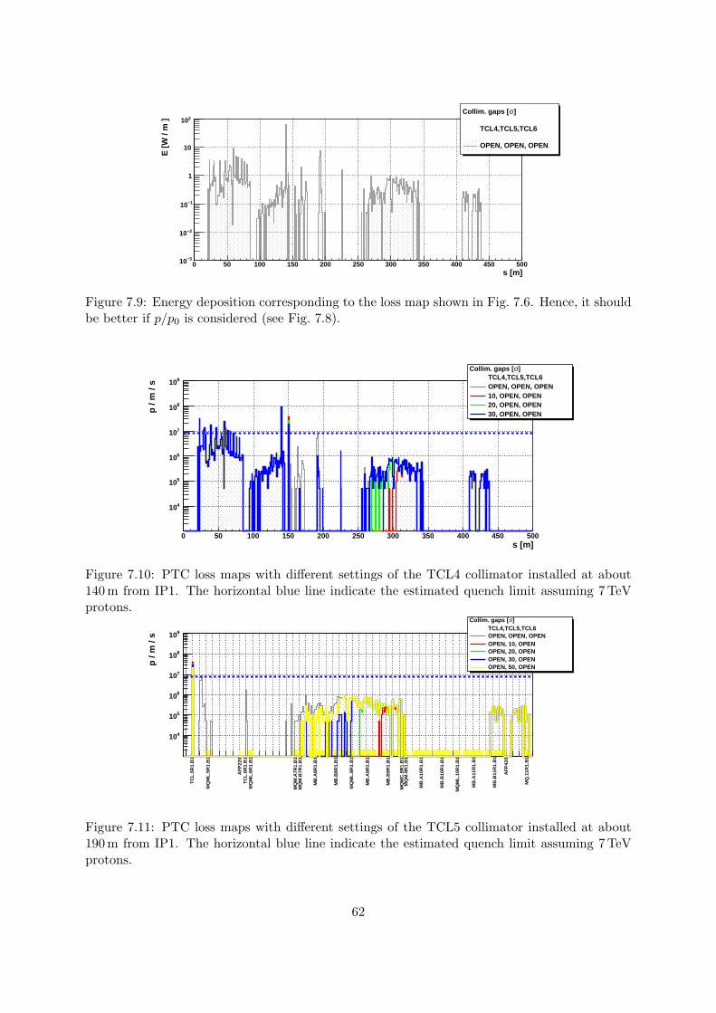
s [m]0 50 100 150 200 250 300 350 400 450 500

E [W

/ m

]

−310

−210

−110

1

10

210]σCollim. gaps [

TCL4,TCL5,TCL6

OPEN, OPEN, OPEN

Figure 7.9: Energy deposition corresponding to the loss map shown in Fig. 7.6. Hence, it shouldbe better if p/p0 is considered (see Fig. 7.8).

s [m]0 50 100 150 200 250 300 350 400 450 500

p / m

/ s

410

510

610

710

810

910

]σCollim. gaps [TCL4,TCL5,TCL6OPEN, OPEN, OPEN10, OPEN, OPEN20, OPEN, OPEN30, OPEN, OPEN

Figure 7.10: PTC loss maps with different settings of the TCL4 collimator installed at about140m from IP1. The horizontal blue line indicate the estimated quench limit assuming 7TeVprotons.

TC

L.5R

1.B

1

MQ

ML.

5R1.

B1

AF

P22

0T

CL.

6R1.

B1

MQ

ML.

6R1.

B1

MQ

M.A

7R1.

B1

MQ

M.B

7R1.

B1

MB

.A8R

1.B

1

MB

.B8R

1.B

1

MQ

ML.

8R1.

B1

MB

.A9R

1.B

1

MB

.B9R

1.B

1

MQ

MC

.9R

1.B

1M

QM

.9R

1.B

1

MB

.A10

R1.

B1

MB

.B10

R1.

B1

MQ

ML.

10R

1.B

1

MB

.A11

R1.

B1

MB

.B11

R1.

B1

AF

P42

0

MQ

.11R

1.B

1

p / m

/ s

410

510

610

710

810

910

]σCollim. gaps [TCL4,TCL5,TCL6OPEN, OPEN, OPENOPEN, 10, OPENOPEN, 20, OPENOPEN, 30, OPENOPEN, 50, OPEN

Figure 7.11: PTC loss maps with different settings of the TCL5 collimator installed at about190m from IP1. The horizontal blue line indicate the estimated quench limit assuming 7TeVprotons.

62

TC

L.5R

1.B

1

MQ

ML.

5R1.

B1

AF

P22

0T

CL.

6R1.

B1

MQ

ML.

6R1.

B1

MQ

M.A

7R1.

B1

MQ

M.B

7R1.

B1

MB

.A8R

1.B

1

MB

.B8R

1.B

1

MQ

ML.

8R1.

B1

MB

.A9R

1.B

1

MB

.B9R

1.B

1

MQ

MC

.9R

1.B

1M

QM

.9R

1.B

1

MB

.A10

R1.

B1

MB

.B10

R1.

B1

MQ

ML.

10R

1.B

1

MB

.A11

R1.

B1

MB

.B11

R1.

B1

AF

P42

0

MQ

.11R

1.B

1

p / m

/ s

410

510

610

710

810

910

]σCollim. gaps [TCL4,TCL5,TCL6OPEN, OPEN, OPEN30, 15, OPEN30, OPEN, 30

Figure 7.12: Comparison between loss maps with the presently foreseen collimation scheme (red)and a first alternative scheme (green) implying the displacement of TCL5 in front of Q6.

TC

L.5R

1.B

1

MQ

ML.

5R1.

B1

AF

P22

0T

CL.

6R1.

B1

MQ

ML.

6R1.

B1

MQ

M.A

7R1.

B1

MQ

M.B

7R1.

B1

MB

.A8R

1.B

1

MB

.B8R

1.B

1

MQ

ML.

8R1.

B1

MB

.A9R

1.B

1

MB

.B9R

1.B

1

MQ

MC

.9R

1.B

1M

QM

.9R

1.B

1

MB

.A10

R1.

B1

MB

.B10

R1.

B1

MQ

ML.

10R

1.B

1

MB

.A11

R1.

B1

MB

.B11

R1.

B1

AF

P42

0

MQ

.11R

1.B

1

p / m

/ s

410

510

610

710

810

910

������������������������������������������������������������������������������������������������������������������������������������������������������������������������������������������������������������������������������������������������������������������������������������������������������������������������������������������������������������������������������������������������������������������������������������������������������������������������������������������������������������������������������������������������

������������������������������������������������������������������������������������������������������������������������������������������������������������������������������������������������������������������������������������������������������������������������������������������������������������������������������������������������������������������������������������������������������������������������������������������������������������������������������������������������������������������������������������������������

]σCollim. gaps [TCL4,TCL5,TCL6OPEN, OPEN, OPEN

������

������

30, OPEN, 3030, 50, 40

Figure 7.13: Comparison between loss maps with a second alternative scheme (green) implyingthe installation of a new collimator in front of Q6 and the first alternative presented in Fig. 7.12.

7.6 Conclusion1562

The analytical calculations and tracking simulations presented in this note provide two alterna-1563

tive collimation schemes to the one presently foreseen in the ATLAS (and CMS) straight section1564

regions. According to these studies, the two alternatives would guarantee the LHC protection1565

from physics debris and enough acceptance for the detectors proposed at 220 meters from the1566

IP. Both alternatives imply the installation of a collimator between the Q5 and Q6 magnets, as1567

close as possible to Q6. This looks possible after studying the present LHC layout and a visual1568

inspection in the tunnel. However, a detailed study of the collimator integration is necessary for1569

validating the proposal.1570

The overall study interpretation depends on the estimated quench limit for the supercon-1571

ducting elements and the early LHC runs will give information about the accuracy of such1572

estimation.1573

Even though the studies considered a perfectly linear model of the LHC optics, the relative1574

comparison among loss maps produced with different collimation schemes is considered accurate.1575

Indeed, the numerical simulations reproduced nicely the results of Baichev-Jeanneret performed1576

63

with a different tracking code and p-p generator. In addition, the two independent codes PTC1577

and SIXTRACK exhibited very consistent results when using the same LHC model in terms of1578

optics and aperture.1579

1580

The absolute simulation accuracy can be improved by considering magnetic field errors mea-1581

sured in the laboratory and magnet elements misalignment measured in the LHC tunnel. The1582

results could also be improved by using the accelerator optics as measured during the early LHC1583

runs.1584

1585

A complete estimation of the effect of the physics debris on the LHC elements can be achieved1586

by modeling the electromagnetic and hadronic showers resulting from the scattering of the of1587

the proton on the TCL. This can be done with Monte Carlo codes such as Geant4 and FLUKA,1588

with the showers initiated from the PTC loss maps in the collimators.1589

64

Chapter 81590

Appendix II: LHC Optics,1591

Acceptance, and Resolution1592

Figure 8.1: chematic view of the beamline at IP1.

8.1 Beamline1593

The configuration of the LHC beamline around the interaction points is shown schematically in1594

Figure 8.1. The proposed forward detector stations are to be installed in the regions located1595

at approximately 220 m from the IP1 interaction point in both beamlines downstream of the1596

central detector. A similar installation is planned for the IP5 region. Protons that have lost1597

energy in the primary interaction are not focussed to travel long distances around the beamline1598

and emerge laterally after passing through bending magnets. At 220m we can observe protons1599

that have lost typically 100 GeV or more in the primary interaction. The acceptance and the1600

ultimately achievable energy resolution of the forward detectors depends on the LHC beam1601

optics and on the position of the detectors relative to the beam.1602

The AFP Collaboration has written a tracking program, FPTrack [58], which has been1603

incorporated into the ATHENA package. It tracks protons (or other particles) that emerge in a1604

forward direction from the interaction region, and tracks them through the system of magnets1605

and collimators that form the beamline, in either direction. FPTrack is much easier and faster1606

to use in this context than the MAD-X program, the standard beam transport program used at1607

65

CERN, and detailed comparisonss have been carried out to ensure that the two programs give1608

results that are in agreement. A model of the LHC beamline optics is implemented, and it can1609

be updated when new beam optics configurations are announced. The CMS collaboration also1610

have their own tracking program and, again, checks have been made that the programs are all1611

equivalent. All calculations presented here are in terms of the planned 7000 GeV beamline.1612

The tracking operates by applying thick-magnet bending using a full momentum-dependent1613

formula at each bemline element. This is essential owing to the non-linearities in the system1614

when off-axis and off-momentum particles are being tracked. Collimators are taken into account,1615

as are the apertures of the beamline elements. Two collimator conditions are considered, “open”,1616

in which the collimators TCL.4, TCL.5 and TCL.6 are opened, and “closed”, in which they are1617

set at positions that have been calculated to protect the beam elements with minimal obstruction1618

to the beam. In this context the configuration “30,50,40” described in Appendix I has been used.1619

It should be noted that the beamline contains dipole and quadrupole magnets only, with1620

no sextupoles. Therefore the horizontal and vertical bending and focussing of the protons are1621

independent of each other. All the most important properties of the beamline of relevance here1622

depend only on the horizontal behaviour of the beam apart from aperture effects, which are1623

fully taken into account in both dimensions.1624

Unless otherwise stated, we use the ExHuME or FPMCMonte Carlo [59] to generate outgoing1625

protons from the central exclusive production of a SM Higgs Boson, although the results will1626

apply for any double-diffractively produced system. Version 6.503 of the LHC optics files have1627

been used with: β∗ = 0.55 m; angular divergence at the IP σθ = 30.2 µrad; crossing angle =1628

142.5 µrad in the vertical (horizontal) plane at IP1 (IP5); beam energy spread σE = 0.77 GeV.1629

The energy spread of the 7000 GeV beam is taken into account and is an irreducible limiting1630

factor on the mass resolution obtainable by proton tagging detectors at the LHC1631

8.2 Detector Acceptance1632

The position and direction of a proton as it hits the 220 m detectors (for a given LHC optics)1633

depend on the energy E and scattering angle θ of the proton as it emerges from the primary1634

interaction, and on the z-vertex position where this occurs, although the latter has a relatively1635

weak effect. The variables E and θ are directly related to ξ, the fractional longitudinal momen-1636

tum loss of the outgoing proton, and −t, the square of the four-momentum transfer. Figure 8.21637

shows the acceptance in the ξ-t plane for the 220 m regions for beam 1 and beam 2 respectively,1638

around IP1. The acceptance is averaged over the azimuthal angle of the emerging proton, and1639

hence can take intermediate values in the range (0., 1.).1640

The acceptance is affected by the collimator settings used. To illustrate this, the figures1641

shows acceptances with the collimators referred to above open and closed. Unless mentioned, all1642

quantities in the present section refer to calculations made with the closed-collimator configura-1643

tion. There are regions of parameter space where the acceptance, averaged over the azimuthal1644

angle of the proton, is excellent, and these are not greatly impacted by the necessary use of the1645

collimators.1646

Figure 8.3 shows the proton distributions in the horizontal coordinate x at 220 m from1647

the interaction point. The distribution is averaged over the proton momentum distribution1648

and depends on the type of physics process that is generating the protons. There are differences1649

between the two beamlines which it is necessary to keep under scrutiny. The upper distributions1650

are obtained as an average over a range of masses of a centrally double-diffractively produced1651

object, between 180 and 1440 GeV. The lower distributions are obtained from a model of the1652

main diffractive processes that are expected to occur in proton-proton interactions at 7000+70001653

66

xi0.05 0.1 0.15 0.2

)2t (

GeV

0

1

2

3

4

0

10

20

30

40

50

60

70

80

90

100

xi0.05 0.1 0.15 0.2

)2t (

GeV

0

1

2

3

4

0

10

20

30

40

50

60

70

80

90

100

xi0.05 0.1 0.15 0.2

)2t (

GeV

0

1

2

3

4

0

10

20

30

40

50

60

70

80

90

100

xi0.05 0.1 0.15 0.2

)2t (

GeV

0

1

2

3

4

0

10

20

30

40

50

60

70

80

90

100

Figure 8.2: Acceptance in the ξ, t plane for protons to reach planes at 220 m in beam 1 (left)and beam 2 (right) around IP1, where ξ is the fractional energy loss of the proton. The variableplotted as t is the modulus of the squared momentum transfer to the proton at the IP and ξits fractional energy loss; no detector effects are included here. Upper (lower) plots: collimatorsopen (closed).

67

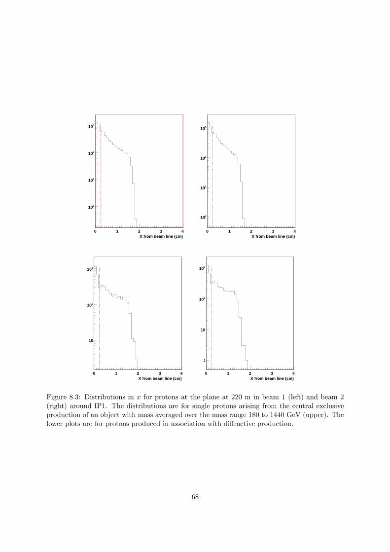
X from beam line (cm)0 1 2 3 4

210

310

410

510

X from beam line (cm)0 1 2 3 4

210

310

410

510

X from beam line (cm)0 1 2 3 4

10

210

310

X from beam line (cm)0 1 2 3 4

1

10

210

310

Figure 8.3: Distributions in x for protons at the plane at 220 m in beam 1 (left) and beam 2(right) around IP1. The distributions are for single protons arising from the central exclusiveproduction of an object with mass averaged over the mass range 180 to 1440 GeV (upper). Thelower plots are for protons produced in association with diffractive production.

68

GeV. These are of physics interest in their own right, but will form a background to any processes1654

of a rarer nature.1655

In order to understand the issues that determine the design of the silicon detector systems,1656

a further set of plots (fig 8.4) shows the x distributions obtained from protons originating from1657

centrally produced objects generated over a selection of masses. The general feature is that at1658

lower masses the protons emerge closer to the beamline, with broader distributions developing1659

as the mass increases. In the plots shown in this figure, a pair of protons in coincidence is not1660

demanded, and just the single protons are plotted, since the probability of a a coincidence is1661

small at masses below about 400 GeV. In fig. 8.5, proton distributions are shown at higher1662

masses with the requirement that a proton is detected in both silicon detector systems. Fig. 8.61663

shows the proton hit distributions for different region in diffractive mass.1664

Fig. 8.7 shows the acceptance of the system for detecting a proton in the 220m systems1665

in both beamlines in coincidence, as a function of the mass of a double-diffractively produced1666

central object X. It varies substantially with the distance of the silicon detectors from the beam,1667

which for convenience is taken here to be the same in both beamlines, although in practice this1668

is not a necessary constraint. As the distance increases, the lower end of the range of accepted1669

masses increases, but the upper end is not affected. The acceptances shown are calculated with1670

our best available model of the collimator settings that could be used.1671

The position of the silicon detectors that we can use will be determined in close collaboration1672

with the accelerator experts, and will need to allow for an inevitable “dead region” occupied by1673

the wall of the movable beam pipe and the edge of the silicon detectors. The permitted distance1674

between the beam and the closest physical material is normally assumed to be 10 times the1675

Gaussian width “sigma” of the beam, where sigma at 220m is 0.09 mm horizontally according1676

to the currently assumed optics. We show results for the separation between the beam and the1677

active silicon detection region having an “optimistic” value of 2 mm, a “realistic” value of 2.51678

mm and a “pessimistic” value of 3 mm.1679

8.3 Momentum determination1680

The mapping of the energy loss and outgoing angle of a proton at the interaction point on to1681

a position and angular measurement in the detector at 220 m or 420 m can be visualized using1682

chromaticity plots. Figure 8.8 shows iso-energy and iso-angle curves for protons with energy1683

loss ranging from 0 to 1000 GeV in steps of 100 GeV at 220 m, evaluated at points in the1684

range ±250µrad in steps of 10 µrad. If the protons were bent out of the beamline in a simple1685

manner, the isoenergetic sets of points would be vertical, corresponding to a fixed value of x for1686

a given proton momentum. However the non-linear nature of the beam optics, involving energy1687

dependence of the transfer matrices, produces chromaticity plots that are very different from1688

such a situation.1689

The chromaticity plots show that the measurement of the energy of the outgoing proton1690

requires good measurements of both position and angle in the detector stations. Thus, at low1691

momentum losses ξ an excellent position measurement is required, whereas the measurement of1692

higher momentum losses becomes increasingly determined by the angular measurement. Hence1693

we shall require detector stations distributed suitably along the space available to us at 220m.1694

Polynomial-based parametrization formulae have been developed in order to evaluate the1695

proton momenta from the measured parameters in the silicon detectors. The formulae are based1696

on fits to the calculated positions and angles, using the generated values of the momentum and1697

emission angle at the IP, and averaging over the width of the beam-beam interaction region.1698

Further development in this area is in hand, using the ALFA code to unfold the initial parameters1699

69

X from beam line (cm)0 1 2 3 4

10

210

310

X from beam line (cm)0 1 2 3 4

1

10

210

310

X from beam line (cm)0 1 2 3 4

10

210

310

X from beam line (cm)0 1 2 3 4

1

10

210

310

X from beam line (cm)0 1 2 3 4

10

210

310

X from beam line (cm)0 1 2 3 4

1

10

210

310

Figure 8.4: Distributions in x for protons at the plane at 220 m in beam 1 (left) and beam 2(right) around IP1. The distributions are for single protons arising from the central exclusiveproduction of an object with mass 180 GeV (upper), 240 GeV (centre), 360 GeV (lower).

70

X from beam line (cm)0 1 2 3

1

10

210

X from beam line (cm)0 1 2 3

1

10

210

X from beam line (cm)0 1 2 3

10

210

310

X from beam line (cm)0 1 2 3

1

10

210

310

X from beam line (cm)0 1 2 3

1

10

210

310

X from beam line (cm)0 1 2 3

1

10

210

310

Figure 8.5: Distributions in x for protons at the plane at 220 m in beam 1 (left) and beam 2(right) around IP1. The distributions are for protons from the central exclusive production ofan object with mass 360 GeV (upper), 480 GeV (centre), 600 GeV (lower). Both protons arerequire to emerge at a distance of at least 2mm from the beam.

71

X from beam line (cm)0 1 2 3

Y fr

om b

eam

line

(cm

)

−2

−1

0

1

XYplanes−1XYplanes−1

X from beam line (cm)0 1 2 3

Y fr

om b

eam

line

(cm

)

−2

−1

0

1

XYplanes+1XYplanes+1

X from beam line (cm)0 1 2 3

Y fr

om b

eam

line

(cm

)

−2

−1

0

1

XYplanes−1XYplanes−1

X from beam line (cm)0 1 2 3

Y fr

om b

eam

line

(cm

)

−2

−1

0

1

XYplanes+1XYplanes+1

X from beam line (cm)0 1 2 3

Y fr

om b

eam

line

(cm

)

−2

−1

0

1

XYplanes−1XYplanes−1

X from beam line (cm)0 1 2 3

Y fr

om b

eam

line

(cm

)

−2

−1

0

1

XYplanes+1XYplanes+1

Figure 8.6: Distributions in x, y for protons at the plane at 220 m in beam 1 (left) and beam2 (right) around IP1. The plots are for objects with mass 360, 480 and 600 GeV (first, secondand third lines) when both protons are detected.

72

Mass of Higgs (GeV)200 400 600 800 1000 1200 1400

Acc

epta

nce

0.0

0.1

0.2

0.3

0.4

0.5

0.6

IP1. 220m + 220m.

Si at2mm 2.5mm3mm

IP1. 220m + 220m.

Figure 8.7: Acceptance as a function of centrally produced mass for 220 + 220 m proton tagsfor the edge of the silicon detector active region located at different distances from the beam.The collimators are closed.

X from beam line (cm)0 1 2 3

dx/d

z (m

rad)

−0.2

0

0.2

XdX+1

X from beam line (cm)0 1 2 3

dx/d

z (m

rad)

−0.2

0

0.2

XdX−1

Figure 8.8: Chromaticity distributions for the 220m detectors in beam 1 (left) and beam 2(right).The radially distributed sets of points are for protons at energies of 6900 GeV, 6800 GeV, etc,starting at the left of each plot and reading clockwise. Within each set, the points denote protonsemerging from the primary interaction at intervals of 10 µrad in the horizontal plane.

73

Mass of Higgs (GeV)200 400 600 800 1000 1200 1400

Res

olut

ion

(GeV

)

0

1

2

3

4

5

6

7

8

9

10IP1. 220m + 220m.

Si at 1.5mm

Si at 3mm

IP1. 220m + 220m.

Mass of Higgs (GeV)200 400 600 800 1000 1200 1400

Res

olut

ion

(GeV

)

0

2

4

6

8

10

12IP1. 220m +220m. Silicon at 1.5mm

(1)

(2)

(3)(4)

rad angular smearingµm linear, 2µ (1) 10 rad angular smearingµm linear, 1µ (2) 10

m linear, no angular smearingµ (3) 10 (4) no measurement smearing

IP1. 220m +220m. Silicon at 1.5mm

Figure 8.9: Reconstructed mass resolution for production of central objects of various masses.First plot: applying nominal measurement resolution and experimental smearings, the resolutionfor two different values of the silicon distance from the beam is compared. Second plot: effect ofvarious values of measurement resolution on the mass resolution. The fluctuations on the curvesare of a statistical origin.

of the forward proton given the final measured parameters.[60]1700

8.4 Mass measurement1701

From the momenta of the pair of oppositely emerging protons in an event, the mass of the1702

centrally produced system can be calculated by a missing-mass formula [61]. The mass resolution1703

was evaluated by a Gaussian fit to the difference of the calculated and input masses. Minimizing1704

this resolution is important for the physics capabilities of the proposed new detectors. For present1705

purposes, we consider protons whose event vertex is at the nominal position of the interaction1706

point. Effects of variations of the x and z are easily included, and we find that they are not1707

large. It is to be noted that the vertex position is well-measured by the central detector for1708

every event, and the average value of x and z for a given run will also be well-measured; both1709

quantities are expected to is expected to be quite stable within a run. Thus offline corrections1710

74

for the mean variations and event-by-event are easily applied.1711

The following factors affect the measured mass resolution of a narrow object produced in1712

the exclusive double diffraction process:1713

• The Gaussian width of the momentum distribution of the circulating proton beam. This1714

is specified as 0.77 GeV.1715

• The lateral uncertainty of the position of the interaction point. This is taken to be 11.8 µm1716

from the intrinsic beam width, but can be improved if the central silicon detector system1717

provides a better measurement on an event-by-event basis.1718

• The angular spread of the interacting beams, corresponding to a lateral momentum smear-1719

ing of 0.21 GeV on the outgoing proton.1720

• The position measurement uncertainty in the detector system1721

• The angular measurement uncertainty in the detector system.1722

Figure 8.9 shows the affect of the above factors on the mass resolution. We first confirm that1723

the resolution is not greatly dependent on the distance of the silicon detectors from the beam,1724

provided that the acceptance is present, by fixing the smearing conditions at some standard1725

values (Item (2) below).We then examine the effects of fixing the silicon distance at a minimum1726

value of 1.5 mm, and varying the smearing that is applied (lower plot):1727

• (1) Applying 10 µm linear and 2 µrad angular smearing on the x measurement of the1728

proton at 220m.1729

• (2) As (1), but with the angular smearing reduced to 1 µrad.1730

• (3) As (1) but with no angular smearing1731

• (4) With no measurement smearings, but including all the intrinsic smearings.1732

It can be seen that an accurate angular measurement is critical, but to achieve a reasonable value1733

of ±1µrad in this quantity, we must measure the positions to high precision. As the momentum1734

loss ξ of the protons emerging from the primary interaction increases, the missing mass increases1735

but the momentum measurement becomes increasingly dependent on the angular measurement,1736

as noted in discussing the chromaticity plots.1737

It is possible to measure the transverse momentum of the proton as it emerges from the1738

interaction point, again by means of polynomial-based parametrization formulae using the mea-1739

surements in the detector stations. Both x and y measurements are required to determine the1740

full transverse momentum of the proton. The measurement is degraded by two factors. The1741

angular beam spread at the interaction points is equivalent to a ± 0.21 GeV transverse mo-1742

mentum spread, both horizontally and vertically, and the poorer measurement uncertainty in1743

the y direction increases the overall uncertainty on pT significantly. Studies are continuing to1744

determine the requirements for particular physics studies and whether they can be achieved.1745

8.5 Calibration1746

Consistent alignment of the silicon system relative to the magnets, the beamline and the exper-1747

imental hall can be achieved by means of beam position monitors, as discussed in the relevant1748

section of this proposal. However to take account of any unknown or unforseen effects, it is1749

75

X from beam line (cm)0 1 2 3

Xse

c fb

per

bin

0

50

100

150

200

250

X from beam line (cm)0 1 2 3

Xse

c fb

per

bin

0

50

100

150

200

250

Figure 8.10: Cross section for detecting a forward proton accompanying a muon pair producedby the photon-photon process in the central detector within a rapidity range of ±2.5. Left,beam 1; right; beam 2; upper, muon pT > 6 GeV. The plotted cross sections are fb per bin in xmeasured in the silicon planes.

necessary to calibrate the momentum measurement of the protons. This can be done by means1750

of the production of lepton pairs, of which muon pairs give best precision, in the central ATLAS1751

detector. Triggers exist that should be able to record events in which a muon pair is produced1752

by the photon-photon process where the photons radiate off the protons. At present, we foresee1753

a trigger on muon pairs where each muon has transverse momentum of at least 6 GeV, however1754

a lower value could be helpful.1755

The accurately measured momenta of the muons allow the momenta of the forward protons1756

to be accurately evaluated. If either of the latter is measured in the respective forward system,1757

its measured momentum can be compared with the value obtained from the muon pairs, and1758

with sufficient statistics a calibration can be achieved. It is not necessary to record both of the1759

forward protons that emerge in any given event.1760

Using the LPAIR program to generate muon pairs produced within an overall rapidity range1761

of ±2.5,we have estimated the rates of calibration events that can be obtained in this way. They1762

are shown in fig. 8.10 and their values should allow a suitable calibration to be made over1763

a period of time: to calibrate a shift of the mean momentum of one-seventh of its measured1764

resoution, 50 events would be required, since the backgrounds will be small. With the silicon1765

distance from the beam at 2.0, 2.5, 3.0 mm, the integrated cross section for each beamline is 43,1766

19, 7.5 fb, respectively, so that integrated luminosities of 1.1, 2.6 and 6.6 fb−1 will be required1767

to make a calibration. Obviously the situation is assisted if the detectors can be moved as close1768

as possible to the beam, which is desirable anyway.1769

Another possible calibration method that we are considering is to use the bremstrahlung1770

photons recorded in the ZDC. The energy of such a photon has been lost by the forward proton,1771

whose energy is thereby calibrated. There are serious backgrounds in this method, however, and1772

it is harder to implement than the muon-pair method, although the cross section is very much1773

higher. Also, the ZDC may be removed, according to current plans; further study is required.1774

76

8.6 Summary1775

The beam optics at LHC allows protons that have lost momentum in a diffractive interaction1776

to emerge from the beam envelope at regions 220 m from the interaction point. By placing1777

silicon detector arrays in these locations we can detect the protons and obtain good acceptance1778

for diffractively produced objects with a wide range of masses above 180 GeV, the precise1779

acceptances depending on how close it is possible to place the detectors relative to the beam.1780

The expected position and angle resolutions for the protons obtained in the silicon stations are1781

expected to yield mass resolutions of around 6 GeV from the proton pair alone.1782

77

Chapter 91783

Appendix III: A possible extension1784

of the AFP project using 420 m1785

detectors1786

In order to detect centrally produced objects in the mass range ∼ 120 GeV it will be necessary1787

to install proton tagging detectors in the cold region of the LHC 420m from the ATLAS IP. The1788

FP420 Collaboration commissioned the CERN design office, working with the TS/MME group1789

to design a cost effective and safe replacement for the 420m connection cryostat. The main1790

design parameters were to provide warm beam pipes and sufficient space to install moveable1791

silicon tracking and fast timing detectors with little or no disruption to the LHC itself. In this1792

chapter, we describe the new connection cryostat design, as weel as the physics motivations of1793

such an extension of our proposal.1794

9.1 Physics program in 220+420 stage1795

With the 420 m extension of the forward proton detecting system, much broader spectrum of1796

physics applications will be reached. A detailed complete description is given in [24]. Here1797

we summarize those topics that were not possible with the 220 m detectors only. As a rule of1798

thumb, the acceptance in ξ for detectors at 220+420 m corresponds to 0.0015 < ξ < 0.1 and is1799

dominated by very low t.1800

9.2 Central Exclusive Production1801

There are three important reasons why CEP is especially attractive for studies of new parti-1802

cles. Firstly, if the outgoing protons remain intact and scatter through small angles then, to a1803

very good approximation, the primary active di-gluon system obeys a Jz = 0, C-even, P-even,1804

selection rule [7]. Here Jz is the projection of the total angular momentum along the proton1805

beam axis. This selection rule readily permits a clean determination of the quantum numbers of1806

any new resonance. Secondly, because the process is exclusive, the energy loss of the outgoing1807

protons is directly related to the invariant mass of the central system, allowing an excellent1808

mass measurement irrespective of the decay mode of the central system [61]. Even final states1809

containing jets and/or one or more neutrinos are measured with σM ∼ 2 GeV/c2. Thirdly, in1810

many topical cases and in particular for Higgs boson production, a signal-to-background ratio of1811

order 1 or better is achievable. This ratio becomes significantly larger for Higgs bosons in certain1812

78

regions of MSSM parameter space [62]. The CEP cross sections in the following discussion are1813

calculated using the KMR model [7].1814

9.2.1 h → bb1815

As an example of what may be possible with ATLAS FP, we briefly review a detailed analysis1816

carried out in [62] of the h → bb channel in a specific MSSM scenario. The MSSM point chosen1817

for this analysis is mA = 120 GeV and tanβ=40. The lightest Higgs boson, h, has a mass1818

of 119.5 GeV and the cross section×branching ratio is approximately 20 fb. ATLAS FP is1819

particularly well suited to observing the Higgs sector in certain regions of MSSM parameter1820

space; at high tanβ the CEP cross sections are in general enhanced with respect to the Standard1821

Model and the branching ratio to bb can be as high as 90% if the light SUSY decay channels1822

are not allowed. Furthermore, the Jz = 0 selection rule suppresses the irreducible bb continuum1823

background significantly, thus enhancing the signal to background ratio with respect to standard1824

search channels. Finally, because the pseudo-scalar A cannot be produced in CEP, ATLAS1825

FP will provide a clean measurement of the mass and quantum numbers of h and H even1826

when mA is close to mh or mH , which can occur at high tanβ. CEP can therefore provide1827

complementary information about the Higgs bosons if the MSSM is realised in nature and could1828

allow a measurement of the Hbb coupling, which may be difficult in other production channels.1829

The challenge is controlling the overlap (or pile-up) background at high luminosity. The1830

primary overlap background consists of a three-fold coincidence in one bunch crossing between1831

an event producing a hard scatter, with the signature of interest detected in ATLAS, and two1832

single diffractive events that produce forward protons within the acceptance of the forward1833

detectors. The overlap background is most problematic for dijet final states because there is1834

a large cross section for non-diffractive dijet production at the LHC. For example, the overlap1835

background to h → bb is estimated to be a factor of 105 (107) larger than the signal for a1836

luminosity of 1033 (1034) cm−2 s−1.1837

There are several techniques that can be employed to reject the overlap background: (i)1838

vertex matching using the di-jet vertex and fast-timing detectors, (ii) topological requirements,1839

(iii) kinematic matching between the di-jet system and central system measured by the forward1840

detectors and (iv) charged track veto which discriminates against the much larger track multi-1841

plicity in non-diffractive events due to multiple parton-parton interactions. The result is that1842

the overlap background in the h → bb channel is negligible up to ∼ 2×1033 cm−2s−1 and smaller1843

than the other backgrounds up to ∼ 5×1033 cm−2 s−1. At instantaneous luminosities up to1844

1034 cm−2 s−1 it becomes desirable to upgrade the fast timing system to a resolution of 5 to 101845

ps.1846

Figure 9.1 (a) shows the expected mass distribution for protons tagged at 420 m for this1847

parameter choice given 60 fb−1 of data collected at 2×1033 cm−2 s−1. The significance is1848

3.5σ. Figure 9.1 (b) shows the same distribution but for 300 fb−1 of data collected equally at1849

7.5×1033 cm−2 s−1 and 1034 cm−2 s−1 and assuming improved timing rejection. The significance1850

increases to 4.5σ.1851

A detailed study of the coverage in the MA−tanβ plane afforded by forward proton detectors1852

at 420m and 220m from the interaction point was carried out in [62] for several benchmark MSSM1853

scenarios. Figure 9.2 shows the 3σ contours for h → bb observation (upper plot) and H → bb1854

observation (lower plot). Curves are shown for 60 fb−1 and 600 fb−1. The 60 fb−1 scenario1855

was presented as 3 years of data taking at ATLAS and CMS at 1033 cm−2 s−1, which was a1856

scenario with negligible overlap background. The 600 fb−1 scenario corresponds to 3 years of1857

data taking by both ATLAS and CMS at 1034 cm−2 s−1. Figure 9.2 shows that a large region of1858

the MA−tanβ can be covered at the 3σ level given enough luminosity. For example, if tanβ = 401859

79

M (GeV)100 110 120 130 140 150

)-1 s

-2cm

33N

eve

nts

(3

year

s at

2x1

0

0

2

4

6

8

10

12

14

16

(a)

M (GeV)100 110 120 130 140 150

))-1 s

-2cm

3310×

at

10

-1N

eve

nts

(30

0 fb

0

5

10

15

20

25

30

(b)

Figure 9.1: Typical mass fits for the 120 GeV/c2 MSSM h → bb for (a) 3 years of data tak-ing at 2× 1033 cm−2 s−1 (60 fb−1, 3.5σ, 10 ps timing) and (b) 1.5 years of data taking at7.5× 1033 cm−2 s−1 and 1.5 years of data taking at 1034 cm−2 s−1 (300 fb−1, 4.5σ, 5 ps timing).

and MA = 120 GeV/c2, then h → bb would be observed with 3.8σ significance with 60 fb−1 of1860

data (upper plot). For tanβ > 30, the significance is 5σ or above. Such a measurement would1861

provide a unique determination of the quantum numbers of the Higgs boson.1862

It is also possible to test for CP-violation in the MSSM Higgs sector. The azimuthal asym-1863

metry in the outgoing tagged protons is expected to be quite sizable in some MSSM scenarios1864

[63, 64]. In addition, the cross sections can become so large in the MSSM that the excellent1865

mass resolution of the forward detectors could allow to distinguish between Higgs bosons that1866

are almost degenerate in mass, as shown for the tri-mixing scenario in [63].1867

9.2.2 h → ττ1868

In the MSSM, the branching ratio of the Higgs bosons to ττ is approximately 10% for MH/A >1869

150 GeV/c2 if the decays to light SUSY particles are not allowed. The τ ’s decay primarily to1870

1-prong (85%) or 3-prong (15%) track topologies; therefore requiring no additional tracks on1871

the ττ vertex is very effective at reducing non-exclusive background.1872

The possibility of observing the Higgs boson through its decay to ττ was investigated in [62],1873

It was shown that the heavy neutral Higgs, H, can be observed at 3σ in this channel across1874

a large area of the MA − tanβ plane; for mA ∼120 GeV, the 3σ contour extends as low as1875

tanβ ∼ 10 and at higher masses, mA ∼ 200 GeV, the ττ channel is observable for tanβ > 40.1876

The light Higgs boson, h, can be observed at 3σ confidence for mA <130 GeV and tanβ > 15.1877

9.2.3 h → 4τ1878

The possibility of a Higgs boson decaying to 4τ arises in the NMSSM, which extends the MSSM1879

by the inclusion of a singlet superfield, S [63]. The Higgs sector of the NMSSM contains three1880

CP-even and two CP-odd neutral Higgs bosons, and a charged Higgs boson. According to [65]1881

the part of parameter space that has no fine-tuning problems results in the lightest scalar Higgs1882

boson decaying predominantly via h → aa, where a is the lightest pseudo-scalar. The scalar1883

Higgs boson has a mass of ∼100 GeV/c2. If the a has a mass of 2mτ . ma . 2mb, which is1884

80

[GeV]Am100 120 140 160 180 200 220 240

βta

n

5

10

15

20

25

30

35

40

45

50

= 115 GeV hM = 125 GeVhM

= 130 GeVhM

= 131 GeVhM

-1L = 60 fb 2 ×, eff. -1L = 60 fb

-1L = 600 fb 2 ×, eff. -1L = 600 fb

[GeV]Am100 120 140 160 180 200 220 240

βta

n

5

10

15

20

25

30

35

40

45

50

= 1

32 G

eV

HM

= 1

40 G

eVHM

= 1

60 G

eVH

M

= 2

00 G

eVH

M

= 2

45 G

eVH

M

-1L = 60 fb 2 ×, eff. -1L = 60 fb

-1L = 600 fb 2 ×, eff. -1L = 600 fb

Figure 9.2: 3σ contours for h → bb (upper plot) and H → bb (lower plot) in the MA - tanβplane of the MSSM within the Mmax

h benchmark scenario (with µ = +200GeV) for differentluminosity scenarios as described in the text. The values of the mass of the Higgs bosons, mh

and MH , are indicated by contour lines. Overlap background considered to be negligible. Thedark shaded (blue) region corresponds to the parameter region that is excluded by the LEPHiggs boson searches.

81

preferred on general theoretical grounds, then the decay channel h → aa → 4τ would become1885

the dominant decay chain. This is not excluded by LEP data and in such a scenario the LHC1886

could fail to discover any of the Higgs bosons [65].1887

It was shown in [66] that the lightest Higgs boson could be discovered in CEP using forward1888

proton detectors at ATLAS. It is expected that approximately 3-4 events will be retained (after1889

all cuts) using a muon trigger of pT > 10 GeV given three years of data taking if the instantaneous1890

luminosity is greater than 1033 cm−2 s−1. The event rates double if a combination of lepton1891

triggers are used [24]. There is no appreciable background. The mass of the h is obtained using1892

the missing mass method to an accuracy of 2 − 3 GeV/c2 (per event). Furthermore, using the1893

kinematic information provided by the forward detectors and the tracking information from the1894

central detector, it is also possible to make measurements of the a mass; in the above scenario1895

the mass measurement is 9.3± 2.3 GeV/c2.1896

9.2.4 Photon-Photon physics1897

The increase in forward detectors acceptance will ensure high rates of dilepton events used1898

for calibration of 420 m detectors and for the luminosity measurement as already discussed1899

Section 2.3.1. The rates for SM WW two-photon production are greatly enhanced and the1900

production can be measured right from the kinematic mass threshold.1901

Easiest to observe experimentally are the fully leptonic decay channels; requiring no addi-1902

tional tracks on the l+ l− vertex, large lepton acoplanarity and large missing transverse momen-1903

tum strongly reduces the backgrounds, such as γγ → τ+τ−. The cross section for events where1904

both W bosons decay into a muon or electron with pT > 25 GeV and a neutrino EmissT > 20 GeV1905

is ∼ 2fb if both protons are tagged in a forward detector at either 220m or 420m [4]. For 30 fb−11906

collected at low luminosity, one would expect approximately 60 events. The double proton tag1907

requirement is necessary at high luminosity in order to efficiently suppress the overlap back-1908

ground from inclusive (partonic) WW production. Thus for 100 fb−1, one would expect 2001909

events with two proton tags. It was shown in [4] that the SM two-photon could be observed at1910

5σ CL with thus 5fb−1of data.1911

It is possible to investigate the higher rate semi-leptonic decay channel, although further1912

studies are required to determine the effect of the overlap background. It was shown in [9] that1913

the production cross section has a sharp turn on at ∼ 2mW , which allows an in situ calibration of1914

the absolute forward detector energy scale to much better than 1% given 100 fb−1 of data. This1915

process is also an interesting probe of the WWγ vertex. The coupling enters the cross section1916

calculation to the fourth power and so should be extracted with less than 1% uncertainty given1917

100 fb−1 of data. This constraint is competitive with the standard measurement from non-1918

diffractive Wγ production and is insensitive to many of the systematics involved in that case.1919

The opportunity to investigate anomalous gauge boson couplings in vector boson pair pro-1920

duction is to some extent possible with 220 mdetectors only. With combined detector acceptance,1921

distributions of the background processes (arising from for example QCD double pomeron ex-1922

change WW production) can be well measured and the contamination in the signal sample can1923

be well determined by cut inversion methods. In this way the background will be determined1924

from data and derived limits on anomalous gauge couplings coupling will be more robust.1925

9.2.5 Supersymmetric particle production1926

Exclusive two-photon production of new charged particles provides a simple mechanism for the1927

production of new physics beyond the Standard Model. Two photon production of SUSY leptons1928

has been investigated in [67] and the cross section for γγ → l+ l− can be as large as 1 fb, while1929

82

Figure 9.3: Distribution of the reconstructed mass for the LM1 SUSY signal and the WWbackground for an integrated luminosity of 100 fb−1.

remaining consistent with the direct search limits from LEP. The production via γγ fusion has1930

the added advantage over standard LHC production mechanisms of being a direct QED process,1931

with minimal theoretical uncertainties.1932

In [67], the two-photon production of charged SUSY pairs is investigated for three benchmark1933

points in mSUGRA/CMSSM parameter space. The two-photon production of e+e−, µ+µ−,1934

τ+τ− and charginos (χ1, χ2) in the fully leptonic decay channels are considered, which means1935

that the final state consists of two leptons and a large amount of missing energy carried by the1936

LSP and, in the case of τ/χ pair production, neutrinos. Around 50 signal events with S/B∼ 21937

in 100 fb−1 are expected depending on the benchmark point chosen. Results for the LM1 SUSY1938

point are shown in Figure 9.3.1939

.1940

9.3 New connection cryostat1941

The LHC dispersion suppressor and arc magnets are placed in one continuous cryostat from the1942

Q7 quadrupole downstream of an IP, all the way to the Q7 quadrupole of the next IR [68].1943

At the position of the missing magnet of the dispersion suppressor, some 420 m downstream1944

of each IP, there is a 14 m long Connection Cryostat (CC) which contains cold beam-pipes,1945

the 2K heat exchanger, or X-line, and various cryo-lines which run throughout the continuous1946

cryostat. The CC also carries the superconducting busbars of the main bending magnets and1947

quadrupoles and nearly 100 superconducting cables for corrector magnets and other systems.1948

83

Figure 9.4: The new connection cryostat for FP420

There are sixteen CCs in the LHC, each made to be as similar as possible to a standard dipole1949

magnet cryostat, at least as far as interconnection and handling are concerned. At this 420 m1950

point, the dispersion function D, with the standard high luminosity optics, is approximately 2 m1951

and hence protons from the IP which have lost around 1% of their momentum are well separated1952

from the circulating beam, as described in Chapter 8. In order to allow the use of near-beam1953

detectors at this 420 m position it is proposed to replace the existing connection cryostats on1954

each side of IP1 with a warm beam-pipe section and a cryogenic bypass. A New Connection1955

Cryostat (NCC) with approximately 8 m of room temperature beam-pipes has been designed1956

using a modified Arc Termination Module (ATM) at each end.1957

In addition to two modified ATMs and warm beam-pipes, the NCC shown in Fig. 9.4 has a1958

small cross section cryostat below the beam-pipes carrying all the cryo-lines and superconduct-1959

ing circuits and a new specially designed cryostat for the X-line. All this is supported by two1960

longitudinal beams to make a single unit which can be directly exchanged for an existing con-1961

nection cryostat. The passage of the X-line through the ATM modules is the main modification1962

needed to the standard ATMs and the geometrical layout of this passage has been arranged to1963

be as far away as possible from the downstream beam-pipe in order to leave adequate space1964

for near-beam detectors and their associated equipment. The cross-section of the NCC, with1965

the space around the beam-pipes available for detectors and associated mechanics, is shown in1966

Fig. 9.5.1967

The existing connection cryostat contains a box structure of lead plates of 15 mm thickness1968

enclosing the two beam-pipes to reduce the radiation field in the tunnel, essentially replacing1969

the shielding provided by the cold mass in a standard arc dipole cryostat. The same thickness of1970

lead shielding will be provided around the warm beam-pipes and detector stations of the NCC.1971

There are also short lengths of cylindrical shielding in the form of collars around the beam-1972

84

Figure 9.5: Cross-section view of the new connection cryostat for FP420

85

pipes at each end of the existing connection cryostat to limit the risk of quenching adjacent1973

superconducting magnets. Similar collars will be incorporated into the modified ATM’s at each1974

end of the NCC in order to ensure that the NCC is at least equal to the existing cryostat in1975

terms of influence on the local radiation fields and quench performance.1976

Normal Days

Warmup from 1.9K to 4.5 K 1

Warmup from 4.5K to 300 K 15

Venting 2

Dismantling interconnection 10

Removal of the connection cryostat 2

Installation of the FP420 cryostat 5

Realization of the interconnections 15

Leak test and electrical test 4

Closing of the vacuum vessel 1

Evacuation/repump 10

Leak test 2

Pressure test 4

Cooldown from 300 K to 4.5 K 15

Cooldown from 4.5K to 1.9 K 3

Total [days] 89

Table 9.1: The estimated time in days required to install one NCC

The final engineering design of the new connection cryostat still has to be completed in the1977

CERN central design office of the TS/MME group. The design aim is to meet or exceed the1978

same specifications as the existing connection cryostat, whilst providing the maximum useable1979

space for the silicon and timing detectors at 420 m. The preliminary design offers acceptable1980

solutions for all cryogenic and mechanical engineering aspects as well as integration into the1981

LHC environment [69, 70]. The final cryogenic performance will depend on the detailed design,1982

but it has already been established that the additional static heat load arising from the two1983

additional cold to warm transitions will be tolerable for the LHC cryogenic system. During1984

LHC operation, simulations show that the NCC actually contributes a slightly lower dynamic1985

heat load than the existing connection cryostat, because in the 8 m long warm section some1986

synchrotron radiation is being absorbed at room temperature.1987

Since the completion of the preliminary design of the NCC the LHC collimation group have1988

finalised their stage II collimator requirements and work has started on the construction of1989

so-called ’cryo-collimators’ for IR3, to be installed in the 2012/2013 long shutdown. The cryo-1990

collimators are to be installed in what are currently cold sections of the LHC and a new cryo1991

by-pass has been designed and is already under construction, based on similar ideas to the1992

NCC [72] as shown in Fig. 9.6. In view of this it is now intended to base the final NCC design1993

on the components of the new LHC cryo by-pass. Because the new collimators must be installed1994

in the shortest possible beam length the original ATM based design used for the NCC has been1995

abandoned and a new cold to warm transition designed in only 1.25 m. The new cryo by-pass1996

provides 1.7 m of warm beampipe for the collimators in an over-all length of 4.2 m. Adapting1997

this new mechanical concept to the NCC design should thus increase the distance available for1998

detector stations by up to two metres, but the increased thermal contraction of the 14 m long1999

NCC, compared to the 4.2 m by-pass, will have to be correctly taken into account and the2000

86

Figure 9.6: Schematic view of the cryo-bypass and collimator (Courtesy of V. Parma).

horizontal displacement of the X-line needed to allow access to the detectors will have to be2001

made by means of dog-legs in the warm section. Both of these modifications should be straight-2002

forward, but will reduce the gain in space along the beamline. It also has to be noted that the2003

cryo by-pass leaves only 100 mm below the beampipes for the collimator support and moving2004

mechanism. This same distance was 250 mm with the preliminary NCC and hence the free2005

space available has to be increased for the final NCC or the moving beampipe system will have2006

to adopt the new collimator support and moving system. The latter solution would be preferable2007

from the LHC machine point of view, but both possible solutions require a detailed engineering2008

study. It has to be noted that the increased distance was needed to allow the detectors to be2009

mounted on a separate table for stability and alignment reasons. Finally it is clear that the2010

construction and installation of the cryo by-passes in the LHC in 2013 will greatly simplify the2011

preparation and work needed to construct and install NCC’s in 2016. While more design work2012

will be needed to finalise the NCC’s, all engineering solutions will have been checked out on2013

the LHC and methods of construction and installation tried and tested. The cost of the NCC’s2014

should also be reduced [71].2015

The cutting and removal of the existing connection cryostat and its replacement by an NCC2016

is very similar to the replacement of a standard LHC dipole and the task has been evaluated2017

by the group responsible for all the LHC interconnections. Table 9.1 shows the sequence of2018

operations and the estimated time needed in normal working days to complete the exchange of2019

a connection cryostat from start of warm-up to being ready for beam. It is thus conceivable2020

that the installation of an NCC cryostat and near-beam detectors could be completed in a three2021

month shutdown. A preliminary study of the transport aspects has shown that adequate tooling2022

exists and it can be expected that the time needed will be in the shadow of other operations2023

shown in Table 9.1. However, the number of Connection Cryostats that can be replaced in any2024

one shutdown will depend on the work load of the interconnection teams.2025

9.4 Summary2026

In summary, a preliminary design for a replacement connection cryostat that would allow near2027

beam detectors to be placed in the 420 m region has been completed, and a final design can2028

profit from the new cryo bypasses being installed in IR3 in 2013. The solution proposed is2029

expected to have an acceptable cryogenic performance and give similar radiation profiles in2030

the region. With the appropriate approvals and funding, two such cryosats could be built and2031

ready for installation in the long shutdown of 2016, with negligible risk to LHC operations and2032

performance for physics.2033

87

Bibliography2034

[1] A. Brandt, B. Cox, C. Royon et al. [AFP Collaboration], “Letter of Intent for ATLAS FP: A2035

Project to Install Forward Proton Detectors at 220 m and 420 m Upstream and Downstream2036

of the ATLAS Detector,” http://jenni.web.cern.ch/jenni/AFP.loi atlas.pdf.2037

[2] http://www-hep.uta.edu/~brandta/ATLAS/AFP/AFP.html2038

[3] V. M. Budnev, I. F. Ginzburg, G. V. Meledin and V. G. Serbo, Phys. Rept. 15 (1974) 181.2039

[4] E. Chapon, O. Kepka, C. Royon, Phys. Rev. D81 (2010) 074003; O. Kepka and C. Royon,2040

Phys. Rev. D 78 (2008) 073005.2041

[5] J. de Favereau de Jeneret et al., arXiv:0908.2020 [hep-ph].2042

[6] A. Bialas and P. V. Landshoff, Phys. Lett. B 256 (1991) 540.2043

[7] V. A. Khoze, A. D. Martin and M. G. Ryskin, Eur. Phys. J. C 23 (2002) 311; V. A. Khoze,2044

A. D. Martin, R. Orava and M. G. Ryskin, Eur. Phys. J. C 19 (2001) 313; A. B. Kaidalov,2045

V. A. Khoze, A. D. Martin and M. G. Ryskin, Eur. Phys. J. C 33, 261 (2004); V. A. Khoze,2046

A. D. Martin and M. G. Ryskin, Eur. Phys. J. C 19 (2001) 477 [Erratum-ibid. C 20 (2001)2047

599].2048

[8] J. R. Cudell, A. Dechambre, O. F. Hernandez, arXiv 1011.3653; J. R. Cudell, A. Dechambre,2049

O. F. Hernandez, I. P. Ivanov, Eur. Phys. J. C 61 (2009), 369; A. Dechambre, O. Kepka,2050

C. Royon, R. Staszewski, arXiv:1101.1439.2051

[9] M. Boonekamp, R. Peschanski, C. Royon, Phys. Rev. Lett. 87 (2001) 251806; Nucl. Phys.2052

B669 (2003) 277; Phys. Lett. B598 (2004)243; M. Boonekamp, A. De Roeck, R. Peschan-2053

ski, C. Royon, Phys. Lett. B550 (2002) 93; M. Boonekamp, C. Royon, J. Cammin and2054

R. B. Peschanski, Phys. Lett. B 654 (2007) 104 [arXiv:0709.2742 [hep-ph]].2055

[10] T. Aaltonen et al. [CDF Run II Collaboration], arXiv:0712.0604 [hep-ex]; T. Aaltonen et2056

al. [CDF Collaboration], Phys. Rev. Lett. 99 (2007) 2420022057

[11] A. Abulencia et al. [CDF Collaboration], Phys. Rev. Lett. 98 (2007) 112001.2058

[12] K. Piotrzkowski, Phys. Rev. D63 (2001) 071502.2059

[13] G. Abbiendi et al. [OPAL Collaboration], Phys. Rev. D 70 (2004) 0320052060

[14] P. J. Bell, Eur. Phys. J. C 64 (2009) 25 [arXiv:0907.5299 [hep-ph]].2061

[15] C. Grojean (CERN & Saclay, IPhT), James D. Wells (CERN & Michigan U., MCTP),2062

private communication.2063

88

[16] A. Brandt et al. [UA8 Collaboration], Phys. Lett. B 297 (1992) 417.2064

[17] V. Barone and E. Predazzi, High-energy particle diffraction, Springer, 2002.2065

[18] S. Alekhin et al., “HERA and the LHC - A workshop on the implications of HERA for LHC2066

physics: Proceedings Part B”, arXiv:hep-ph/0601013.2067

[19] M. Arneodo and M. Diehl, “Diffraction for non-believers”, hep-ph/0511047 (2005).2068

[20] M. Albrow et al. [CMS and TOTEM Collaborations], CERN-LHCC-2006-039; The2069

FP420 R&D Project: Higgs and New Physics with forward protons at the2070

LHC, JINST 4 T10001, hep-ex/0806.0302 (June 2008), accepted in J. Inst.:2071

http://www.iop.org/EJ/abstract/1748-0221/4/10/T10001.2072

[21] M. Deile et al., arXiv:1002.3527 [hep-ph], page 6.2073

[22] V. A. Khoze, A. D. Martin and M. G. Ryskin, Eur. Phys. J. C 18 (2000) 167 [arXiv:hep-2074

ph/0007359].2075

[23] K.Piotrzkowski, U. Schneekloth, Proc. of the ZEUS Collaboration Meeting, March 1994,2076

DESY, Hamburg.2077

[24] M. G. Albrow et al. [FP420 R&D Collaboration], arXiv:0806.0302 [hep-ex].2078

[25] A. Guerrero et al.,“CERN front-end software architecture for accelerator controls,”2079

(ICALEPCS 2003), Korea, Oct 2003. in Gyeongju 2003, Accelerator and large experimental2080

physics control systems, p. 342.2081

[26] M. Slater et al., “Cavity BPM tests for the ILC energy spectrometer”, SLAC-PUB-13031.2082

[27] S. Walston et al., “Performance of a High Resolution Cavity Beam Position Monitor Sys-2083

tem”, unpublished.2084

[28] CERN-LHCC-2010-013 / ATLAS-TDR-019 5/09/2010 https://espace.cern.ch/atlas-2085

ibl/Shared%20Documents/ATLAS-TDR-019.pdf; http://indico.cern.ch/conferenceDisplay.py?confId=1275652086

[29] T. E. Hansen et al., First Fabrication of Full3D Detectors at SINTEF, JINST 4 (2009)2087

P03010.2088

[30] G. Pellegrini et al., First Double-Sided 3-D Detectors Fabricated at CNM-IMB, Nucl. Inst.2089

Meth. A592 (2008) 38.2090

[31] S. Parker, C. Kenney and J. Segal, 3D-A proposed New Architecture for Solid-State Radi-2091

ation Detectors, Nucl. Inst. Meth. A395 (1997) 328.2092

[32] C. Kenney et al., Silicon detectors with 3-D electrode arrays: fabrication and initial test2093

results, IEEE Tr. Nucl. Sci 46 (1999) 1224.2094

[33] M. Mathes et al., Test Beam Characterizations of 3D Silicon Pixel Detectors, IEEE Tr.2095

Nucl. Sci 55 (2008) 3731.2096

[34] P.O. Hansson et al., 3D Silicon Pixel Sensors: Recent Test Beam Results, Nucl. Inst. Meth.2097

A321 (2010).2098

[35] C. Da Via et al., 3D Active Edge Silicon Sensors with Different Electrode Configurations:2099

Radiation Hardness and Noise Performance, Nucl. Inst. Meth. 604 (2009) 505.2100

89

[36] G. Aad et al., ATLAS Pixel Detector Electronics and Sensors, JINST 3 (2008) P07007.2101

[37] A. Lounis et al., TCAD Simulations of the ATLAS Pixel Ring and Edge Structure for2102

SLHC Upgrade, Internal Report ATL-UPGRADE-PUB-2010-001, ATL-COM-UPGRADE-2103

2009-013, CERN, Geneva, Jan 2010.2104

[38] G. Kramberger et al., Comparison of Pad Detectors Produced on Different Silicon Materials2105

after Irradiation with Neutrons, Protons and Pions, Nucl.Inst.Meth. A 612 (2010) 288.2106

[39] L. Andricek et al., Processing of Ultra-Thin Silicon Sensors for Future Linear Collider2107

Experiments, IEEE Tr. Nucl. Sci 51 (2004) 1117.2108

[40] L. Andricek et al., Nucl. Inst. Meth. (2010) in press, In Proc. of 7th International Hiroshima2109

Symposium on Development and Applications.2110

[41] I. Mandic et al., Observation of Full Charge Collection Efficiency in Heavily Irradiated n+p2111

strip Detectors Irradiated up to 3 x 10**15 n(eq)/cm2, Nucl. Inst. Meth. A612 (2010) 474.2112

[42] G. Casse et al., Enhanced Efficiency of Segmented Silicon Detectors of Different Thicknesses2113

After Proton Irradiations up to 1x10**16 n(eq)/cm2, Nucl. Inst. Meth. In Press (2010).2114

[43] E. Mandelli et al., IEEE Trans. Nucl. Sci. 49 (4) (2002) 1774.2115

[44] L. Blanquart et al., IEEE Trans. Nucl. Sci. 49 (4) (2002) 1778.2116

[45] L. Blanquart et al., IEEE Trans. Nucl. Sci. 51 (4) (2004) 1358.2117

[46] ATLAS Collab., JINST 3 (2008) P07007.2118

[47] CMS Collab., NIM A 552 (2005) 232.2119

[48] P-909: http://www.cdf.fnal.gov/upgrades/btb.proposal.ps.2120

[49] M. Akatsu, et al., Nucl. Instr. and Meth. A 440 (2000) 124; M. Akatsu, et al., Nucl. Instr.2121

and Meth. A 528 (2004) 763; Y. Enari, et al., Nucl. Instr. and Meth. A 547 (2005) 490.2122

[50] L. Bonnet, T. Pierzchala, K. Piotrzkowski, P. Rodeghiero. Acta Phys. Polon. B38 (2007)2123

477-482; hep-ph/0703320.2124

[51] CERN/LHCC 2002-016 Addendum to the ALICE TDR 8, 24 April 2002.2125

[52] http://www.nightvision.com/products/military/case study-gen3.htm2126

[53] N. Kishimoto, et al., Nucl. Instr. and Meth. A 564 (2006) 204; T. Mori, “Life-2127

time of HPK Square-shape MCP-PMT,” Cracow Fast Timing Workshop, Dec. 20102128

(http://www-d0.fnal.gov/~royon/timing cracow/).2129

[54] I. Baichev, J.-B. Jeanneret and G.R. Stevenson, Beam losses far downstream of the high2130

luminosity interaction points of LHC - intermediate results, LHC-Project Note 208, CERN,2131

20002132

[55] E. Forest, F. Schmidt and E. McIntosh, “Introduction to the Polymorphic Tracking Code”,2133

CERN-SL-2002-044-AP, KEK report 2002-3, July 2002.2134

[56] R. Assmann et al, The proceedings of PAC03, pag. 3496.2135

90

[57] The LHC design report, CERN-2004-003 (2004)2136

[58] P.J. Bussey and W. Plano, FPTrack, in preparation.2137

[59] J. Monk and A. Pilkington, Comput. Phys. Commun. 175 (2006) 232 [arXiv:hep-2138

ph/0502077]; M. Boonekamp, A. Dechambre, V. Juranek, O. Kepka, M. Rangel, C. Royon,2139

R. Staszewski, [arXiv:1102.2531].2140

[60] R Staszewski et al,. ATL-COM-LUM-2009-016, Nucl. Instr. Meth. A609 (209) 1362141

[61] M. G. Albrow and A. Rostovtsev, arXiv:hep-ph/0009336.2142

[62] B. Cox, F. Loebinger, A. Pilkington, JHEP 0710 (2007) 090; S. Heinemeyer et al.,2143

Eur. Phys. J. C 53 (2008) 231.2144

[63] J. R. Ellis, J. F. Gunion, H. E. Haber, L. Roszkowski and F. Zwirner, Phys. Rev. D 392145

(1989) 844; J. R. Ellis, J. S. Lee and A. Pilaftsis, Phys. Rev. D 71 (2005) 075007 [arXiv:hep-2146

ph/0502251].2147

[64] V. A. Khoze, A. D. Martin and M. G. Ryskin,2148

[65] R. Dermisek, J.F. Gunion. Phys. Rev. Lett. 95 (2005) 041801. Eur. Phys. J. C 34 (2004)2149

3272150

[66] J. R. Forshaw, J. F. Gunion, L. Hodgkinson, A. Papaefstathiou and A. D. Pilkington, JHEP2151

0804 (2008) 090 [arXiv:0712.3510 [hep-ph]].2152

[67] J. Ohnemus, T.F. Walsh and P.M. Zerwas, Phys. Lett. B328 (1994) 369-373; G. Bhat-2153

tacharya et al., Phys. Rev. D 53, (1996) 2371; M. Drees et al., Phys. Rev. D 50, (1994)2154

2335; N. Schul and K. Piotrzkowski, arXiv:0806.1097.2155

[68] “LHC Design Report Vol. 1”, CERN-2004-003, CERN, Geneva, Switzerland (2004).2156

[69] T. Columbet, “Cryogenics preliminary calculation for the FP420 cryostat”,2157

https://edms.cern.ch/document/827775.2158

[70] S. Pattalwar et al. “A New Connection Cryostat to insert FP420 Proton Tagging Detectors2159

in the LHC Ring”, Proceeds APAC (2007) 103.2160

[71] R. Folch, “FP420 Cryostat Modules Workpackage”,2161

https://edms.cern.ch/document/823322.2162

[72] V. Parma, talk at the Chamonix Workshop, January 2011.2163

91