
Affine dual equivalence and k-Schur functions
57
Journal of Combinatorics Volume 3, Number 3, 343–399, 2012 Affine dual equivalence and k -Schur functions Sami H. Assaf ∗ and Sara C. Billey † The k-Schur functions were first introduced by Lapointe, Lascoux and Morse [18] in the hopes of refining the expansion of Macdonald polynomials into Schur functions. Recently, an alternative defini- tion for k-Schur functions was given by Lam, Lapointe, Morse, and Shimozono [17] as the weighted generating function of starred strong tableaux which correspond with labeled saturated chains in the Bruhat order on the affine symmetric group modulo the symmetric group. This definition has been shown to correspond to the Schubert basis for the affine Grassmannian of type A [15] and at t = 1 it is equivalent to the k-tableaux characterization of Lapointe and Morse [22]. In this paper, we extend Haiman’s dual equivalence relation on standard Young tableaux [12] to all starred strong tableaux. The elementary equivalence relations can be interpreted as labeled edges in a graph which share many of the properties of Assaf’s dual equivalence graphs. These graphs display much of the complexity of working with k-Schur functions and the interval structure on S n /S n . We introduce the notions of flattening and squashing skew starred strong tableaux in analogy with jeu de taquin slides in order to give a method to find all isomorphism types for affine dual equivalence graphs of rank 4. Finally, we state some open problems on other ways to generalize dual equivalence. 1. Introduction Classically, the Schur functions have played a central role in the theory of symmetric functions [27]. They also appear in geometry as representatives for Schubert classes in the cohomology rings of Grassmannian manifolds, and they appear in representation theory as the Frobenius characteristics of irreducible S n representations and as the trace for certain irreducible GL n representations. In [18], Lapointe, Lascoux, and Morse introduced a new larger fam- ily of symmetric functions which includes the Schur functions, namely the arXiv: 1201.2128 ∗ Supported by an NSF postdoctoral fellowship. † Supported by grants DMS-0800978 and DMS-1101017 from the NSF. 343
Transcript of Affine dual equivalence and k-Schur functions

Journal of Combinatorics
Volume 3, Number 3, 343–399, 2012
Affine dual equivalence and k-Schur functions
Sami H. Assaf∗and Sara C. Billey
†
The k-Schur functions were first introduced by Lapointe, Lascouxand Morse [18] in the hopes of refining the expansion of Macdonaldpolynomials into Schur functions. Recently, an alternative defini-tion for k-Schur functions was given by Lam, Lapointe, Morse,and Shimozono [17] as the weighted generating function of starredstrong tableaux which correspond with labeled saturated chainsin the Bruhat order on the affine symmetric group modulo thesymmetric group. This definition has been shown to correspondto the Schubert basis for the affine Grassmannian of type A [15]and at t = 1 it is equivalent to the k-tableaux characterizationof Lapointe and Morse [22]. In this paper, we extend Haiman’sdual equivalence relation on standard Young tableaux [12] to allstarred strong tableaux. The elementary equivalence relations canbe interpreted as labeled edges in a graph which share many of theproperties of Assaf’s dual equivalence graphs. These graphs displaymuch of the complexity of working with k-Schur functions and theinterval structure on Sn/Sn. We introduce the notions of flatteningand squashing skew starred strong tableaux in analogy with jeu detaquin slides in order to give a method to find all isomorphismtypes for affine dual equivalence graphs of rank 4. Finally, we statesome open problems on other ways to generalize dual equivalence.
1. Introduction
Classically, the Schur functions have played a central role in the theory ofsymmetric functions [27]. They also appear in geometry as representativesfor Schubert classes in the cohomology rings of Grassmannian manifolds,and they appear in representation theory as the Frobenius characteristics ofirreducible Sn representations and as the trace for certain irreducible GLn
representations.In [18], Lapointe, Lascoux, and Morse introduced a new larger fam-
ily of symmetric functions which includes the Schur functions, namely the
arXiv: 1201.2128∗Supported by an NSF postdoctoral fellowship.†Supported by grants DMS-0800978 and DMS-1101017 from the NSF.
343
344 Sami H. Assaf and Sara C. Billey
k-Schur functions, with similar connections both to geometry and to rep-resentation theory. The k-Schur functions were defined in hopes of refiningand ultimately proving the Macdonald Positivity Conjecture [26]. Precisely,Lapointe, Lascoux, and Morse conjectured that the Macdonald polynomialsexpand into k-Schur functions with polynomial coefficients in two parame-ters q, t with nonnegative integer coefficients, and that the k-Schur functionsexpand into Schur functions with polynomial coefficients with parameter tand nonnegative integer coefficients. Haiman [11] has since shown that theMacdonald polynomials are the Frobenius characteristic of a bigraded Sn-module defined by Garsia and Haiman [7] using the geometry of the Hilbertscheme of points in the plane. This resolved the n! Conjecture and providedthe first proof of Macdonald positivity.
At this time, a number of conjecturally equivalent definitions for k-Schurfunctions exist [17, 18, 19, 20, 21, 22], making the term “k-Schur function”rather ambiguous. In this paper, we advocate for the geometrically inspireddefinition as the weighted generating function of starred strong tableaux pre-sented by Lam, Lapointe, Morse and Shimozono [17]. This definition at t = 1is equivalent to the k-tableaux characterization in [22] which has been shownto represent the Schubert basis in the homology of the affine Grassmannianof type A [15]. Furthermore, the starred strong tableaux are a natural gen-eralization of standard tableaux which appear throughout combinatorics.
Recently, Lam, Lapointe, Morse and Shimozono proved that the k-Schurfunctions as defined below except with t = 1 are Schur positive [16]. Theirapproach shows how k-Schur functions relate to k+1-Schur functions whenthe t is not included.
It is an open problem to show that the k-Schur functions including thet statistic are Schur positive. Toward proving this conjecture, we define afamily of involutions on starred strong tableaux which generalize Haiman’selementary dual equivalence moves on standard Young tableaux [12]. Usingthese involutions, one can put a graph structure on starred strong tableauxwhich satisfies many of the same axioms as the dual equivalence graphs de-fined by the first author in [1]. As our model for dual equivalence is basedon the poset of n-cores induced from Young’s lattice, our results extend tok-Schur functions indexed by skew shapes. Our main result is that thesegraphs, which we call affine dual equivalence graphs, are locally Schur pos-itive when restricted to edges of 2 adjacent colors and the spin is constanton connected components, see Definition 4.5 and Theorem 7.15.1
1Earlier, we announced the stronger result that k-Schur functions as defined hereare Schur positive. However, we have since realized that the proof is incomplete

Affine dual equivalence and k-Schur functions 345
Jeu de taquin is an important algorithm in the theory of symmetric func-tions related to Littlewood-Richardson coefficients. One of the properties ofjeu de taquin slides is that they commute with elementary dual equivalencemoves on tableaux [12, Lemma 2.3]. There is no known analog of jeu detaquin for k-Schur functions at this time. Such an analog would in princi-ple be useful for multiplying k-Schur functions and expanding again intok-Schurs. One approach to finding such a jeu de taquin algorithm is to lookfor sliding moves which commute with affine dual equivalence moves. In Sec-tions 7.1 and 7.2, we describe two types of collapsing moves which commutewith affine dual equivalence in specified cases. These collapsing moves arethe analogs of removing empty rows and columns in a skew tableau via jeude taquin.
One of the main consequences of our results is a connection betweenk-Schur functions and LLT polynomials which is realized by comparing thegraphs for the two functions. We expect that a better understanding of theseconnections will ultimately show that an LLT polynomial expands into k-Schur functions with coefficients that are polynomials in t with nonnegativeinteger coefficients for an appropriate value of k. Given Haglund’s formulaexpanding Macdonald polynomials positively into certain LLT polynomials[9, 10], this would also establish the missing connection between Macdonaldpolynomials and k-Schur functions.
The outline of the paper goes as follows. In Section 2, we review the basicvocabulary on partitions, the affine symmetric group, symmetric functionsand quasisymmetric functions. In particular, we review an interesting orderpreserving bijection between a quotient of the affine symmetric group withthe n-core partitions relating Bruhat order to a subposet of Young’s lattice.In Section 3, one definition of k-Schur functions expanded into fundamen-tal quasisymmetric functions is given following [17, Conjecture 9.11]. Thesefunctions can be indexed by n-cores, minimal length coset representatives forSn/Sn, or k = n− 1 bounded partitions since all three sets are in bijection.In Section 4, we review dual equivalence on standard Young tableaux alongwith the associated graph structures and axioms. In Section 5, we carefullystudy the covering relations and the rank two intervals in the poset on n-core partitions. In Section 6, we define the affine analog of dual equivalenceoperations and prove the key result that these maps are involutions whichpreserve the spin statistic. In Section 7, we use these maps to define the
for two reasons. First, the proof outline requires one to identify all isomorphismtypes for 3-colored components in affine dual equivalence graphs. Our computerverification relies on a halting problem which has not terminated. Second, the axiom(4’) required in [1] is not known to hold for affine dual equivalence graphs.

346 Sami H. Assaf and Sara C. Billey
affine dual equivalence graph on starred strong tableaux of a given shape.In particular, Theorem 7.15 spells out some of the useful properties of thesegraphs. In Section 8, we mention some open problems on other generaliza-tions of dual equivalence graphs. Finally, in the Appendix, we have includedsome examples of k-Schur functions expanded both in quasisymmetric func-tions and Schur functions along with their affine dual equivalence graphs.
2. Basic definitions and notations
2.1. Partitions
A partition λ is a weakly decreasing sequence of non-negative integers
λ = (λ1, λ2, . . . , λl), λ1 ≥ λ2 ≥ · · · ≥ λl > 0.
The Young diagram of a partition λ is the set of points (i, j) in N× N suchthat 1 ≤ i ≤ λj . We draw the diagram so that each point (i, j) is representedby the unit cell southwest of the point. Abusing notation, we will write λ forboth the partition and its diagram. For example, the diagram of (4, 3, 1) is
.
We may also represent λ by an infinite binary string as follows. Considerthe diagram of λ lying in the N× N plane with infinite positive axes. Walkin unit steps along the boundary of λ, writing 1 for each vertical step and 0for each horizontal step. For example, (4, 3, 1) becomes
· · · 1 1 1 0 1 0 0 1 0 1 0 0 0 · · · .
Note that this establishes a bijective correspondence between partitions anddoubly infinite binary strings s such that si = 1 for all i < l and si = 0 forall i > r for some l, r ∈ Z.
For partitions λ, μ, we write μ ⊂ λ whenever the diagram of μ is con-tained within the diagram of λ; equivalently μi ≤ λi for all i. Young’s latticeis defined by the partial ordering on partitions given by containment.
A standard Young tableau of shape λ is a saturated chain in Young’slattice from the empty partition to λ. As moving from rank i− 1 to rank iadds a single box, filling this added box with the letter i uniquely records thechosen chain. Therefore standard Young tableaux are also characterized as
Affine dual equivalence and k-Schur functions 347
bijective fillings of the cells of λ with the letters 1 tom so that entries increase
along rows and up columns. Let SYT(λ) denote the set of all standard
Young tableaux of shape λ, and let SYT denote the union of all SYT(λ).
For example, two standard tableau of shape (4, 3, 1) are
.(2.1)
When μ ⊂ λ, we may define the skew diagram λ/μ to be the set theoretic
difference λ−μ. A standard tableau of skew shape λ/μ is a saturated chain in
Young’s lattice from μ to λ, or, equivalently, a bijective filling of the cells of
λ/μ with entries 1 to m so that entries increase along rows and up columns.
An addable cell for a partition λ is any cell c such that c ∪ λ is again a
Young diagram of a partition. Similarly, a removable cell for a partition λ
is any cell c such that λ− c is again a Young diagram of a partition.
A connected skew diagram is one where exactly one cell has no cell im-
mediately north or west of it, and exactly one cell has no cell immediately
south or east of it. Two distinct connected components can meet at one
point but not along an edge of a cell. A connected skew diagram is neces-
sarily nonempty. A ribbon is a connected skew diagram containing no 2× 2
subdiagram. We may define addable and removable ribbons of λ just as with
cells; namely, a ribbon R is an addable (resp. removable) ribbon for a par-
tition λ if λ ∪R (resp. λ−R) is again a partition.
To each cell x of a diagram λ associate the content of x defined by
c(x) = i − j where the cell x lies in row j and column i. We also consider
the residue of x, defined as the content of x modulo n. The content and
residue of ribbons are defined with respect to the southeasternmost cell.
The head of a ribbon is its southeasternmost cell, and the tail of a ribbon
is its northwesternmost cell.
The hook length of x is the number of squares above and to the right of x
in λ including x itself. Define the bandwidth of a partition to be the number
of distinct contents occupied by its cells. Equivalently, the bandwidth of a
non-skew partition is its maximum hook length.
An n-core is a partition having no removable ribbon of length n. Equiv-
alently, no hook length of λ is divisible by n. Young’s lattice restricted to
n-cores gives another ranked partial order, but it is not a lattice. This partial
order on n-cores is central to the definition of k-Schur functions and strong
tableaux given in Section 3.

348 Sami H. Assaf and Sara C. Billey
2.2. Affine permutations
Here we briefly recall the necessary vocabulary on affine permutations. For a
more thorough treatment of the combinatorial aspects of Coxeter groups we
recommend [5], specifically see Section 8.3 for details on the affine symmetric
group. Recent developments on core partitions and connections to affine
Weyl groups can be found in [4, 13].
Given n, consider the set Sn of all bijections w : Z −→ Z such that
w(i+ n) = w(i) + n ∀i ∈ Z and w(1) + w(2) + · · ·+ w(n) =(n+12
).
For example, given i, j ∈ Z such that i ≡ j (all congruences should be taken
modulo n throughout the paper), the affine transposition ti,j ∈ Sn is the
periodic bijection such that ti,j(i+ p ·n) = j+ p ·n, ti,j(j+ p ·n) = i+ p ·n,and ti,j(k) = k for all k ≡ i and k ≡ j and all p ∈ Z. Sn is known as
the affine symmetric group. It is the affine Weyl group of type An−1. As a
Coxeter group, Sn is generated by the adjacent transpositions si = ti,i+1
for 0 ≤ i < n. If w = si1si2 · · · sip ∈ Sn and p is minimal among all such
expressions for w, then si1si2 · · · sip is a reduced expression for w and the
length of w is p, denoted �(w) = p. The length function is the rank function
for the Bruhat order on Sn. As a partial order, Bruhat order can be described
as the transitive closure of the relation w < ti,jw if �(w) < �(ti,jw). The
symmetric group Sn can be viewed as the parabolic subgroup of Sn generated
by s1, . . . , sn−1.
Let Qn be the minimal length coset representatives for the quotient
Sn/Sn. Bruhat order restricted to Qn is again a partial order ranked by the
length function. There is a rank preserving bijection from n-core partitions
to Qn which respects the Bruhat order. This correspondence leads to useful
criteria for Bruhat order on Qn in Theorem 2.3 and the covering relation in
Proposition 5.3 and Corollary 5.4. We follow [29] for terminology on partial
orders.
Definition 2.1. [14, 21, 28] Define the function
(2.2) C : Qn −→ n-core partitions
recursively as follows. Associate the empty partition with the identity in Qn;
namely, C(id) = ∅. If C(w) = λ and �(siw) > �(w), then C(siw) is obtainedfrom λ by adding every addable cell with residue i to λ.

Affine dual equivalence and k-Schur functions 349
In [14, 21], C is shown to be a bijection. Denote C−1 by
(2.3) A : n-core partitions −→ Qn.
Remark 2.2. Definition 2.1 can be used as an algorithm for generating n-core partitions. The reader is encouraged to look ahead to Figure 1 to seehow the 3-core partitions up to rank 4 are generated.
Note that if λ is an n-core with an addable cell of residue i, then λ hasno removable cells of residue i. Similarly, if λ is an n-core with a removablecell of residue i, then λ has no addable cells of residue i [21, §5].
The following beautiful theorem of Lascoux shows the power of the n-core model for Qn.
Theorem 2.3. [23] Given v, w ∈ Qn, let μ = C(v) and λ = C(w) be thecorresponding n-core partitions. Then μ ⊂ λ in Young’s lattice if and onlyif v < w in Bruhat order restricted to Qn.
2.3. Symmetric and quasisymmetric functions
We adopt notations for the standard bases for Λ, the ring of symmetricfunctions, from [27]. For this paper, we are primarily interested in the Schurfunctions sλ, indexed by partitions. The Schur functions form an orthonor-mal basis for Λ with the Hall scalar product. The Schur functions also givethe irreducible characters for representations of the general linear group aswell as the Schubert basis for the cohomology of the Grassmannian [6].
We will use the expansion for Schur functions in terms of Gessel’s fun-damental quasisymmetric functions [8] rather than in terms of monomialson an alphabet X = {x1, x2, . . .}. The k-Schur functions will have a similarexpansion, presented in Section 3.3.
Definition 2.4. For σ ∈ {±1}m−1, the fundamental quasisymmetric func-tion associated to σ, denoted Qσ, is given by
(2.4) Qσ(X) =∑
i1≤···≤imij=ij+1⇒σj=+1
xi1 · · ·xim .
To connect quasisymmetric functions with Schur functions, for T a stan-dard tableau on 1, . . . ,m, define the descent signature σ(T ) ∈ {±1}m−1 by(2.5)
σi(T ) =
{+1 if the content of i is less than the content of i+ 1,−1 if the content of i+ 1 is less than the content of i.
}

350 Sami H. Assaf and Sara C. Billey
Note that in a standard tableau, consecutive entries may never appear along
the same diagonal so the content of the cells containing i and i+1 are never
equal. In particular, σ is well-defined on SYT.
Theorem 2.5. [8] The Schur function sλ can be expressed in terms of qua-
sisymmetric functions by
sλ(X) =∑
T∈SYT(λ)
Qσ(T )(X).(2.6)
By Theorem 2.3, working with quasisymmetric functions instead of mono-
mials affords us the benefit of working with standard objects instead of semi-
standard objects. Furthermore, the expansion in (2.6) is independent of the
size of the alphabet X which could be finite or infinite.
3. k-Schur functions
In this section, we recall two analogs of standard Young tableaux for the
n-core poset called strong tableaux and starred strong tableaux from [17].
The spin statistic is defined on starred strong tableaux. These ingredients
are combined to give the definition of k-Schur functions in terms of their
expansion into fundamental quasisymmetric functions.
3.1. Strong tableaux
Consider the poset on n-core partitions induced from Young’s lattice. A
strong tableau of shape λ is a saturated chain
∅ ⊂ λ(1) ⊂ λ(2) ⊂ · · · ⊂ λ(m) = λ
in the n-core poset from the empty tableau to λ. We denote this chain by
the filling S of λ where all cells of λ(i)/λ(i−1) contain the letter i.
For example, from Figure 1, the strong tableaux for n = 3 of size m = 4
are
.

Affine dual equivalence and k-Schur functions 351
Figure 1: Poset of 3-cores up to rank 5.
3.2. Starred strong tableaux
A starred strong tableau, S∗, is a strong tableau S where one connectedcomponent of the cells containing i is chosen for each i, and the south-easternmost cell of the chosen components are adorned with a ∗. There-fore, the information contained in S∗ is equivalent to the pair (S, c∗) wherec∗ = (c1, c2, . . . , cm) is the content vector, namely ci is the content of the cellcontaining i∗.
Let SST∗(λ, n) be the set of all starred strong tableaux of shape λ re-garded as an n-core. For example, the 6 starred strong tableaux of shapeλ = (2, 2, 1, 1) are
.(3.1)
The following statistics on a starred strong tableau S∗ were first intro-duced in [17]. Let n(i) denote the number of connected components of thecells containing i of the underlying tableau S. Among such connected com-ponents, let h(i) be the height, i.e. number of rows, of the starred connected

352 Sami H. Assaf and Sara C. Billey
component. Finally, let d(i∗) denote the depth of i∗ in S∗, defined to be the
number of components northwest of the component containing i∗. Define
the statistic spin on starred strong tableaux as follows,
(3.2) spin(S∗) =∑i
n(i) · (h(i)− 1) + d(i∗).
For example, the spins of the starred strong tableaux in equation (3.1), from
left to right, are 0, 1, 1, 2, 1, 2.
This spin statistic was dubbed “spin” based on similarities with the spin
statistic on ribbon tableaux that gives LLT polynomials [24]. We explore
deeper connections between LLT polynomials and k-Schur functions in Sec-
tion 8.
3.3. Quasisymmetric expansion
The k-Schur function s(k)λ (X; t) is the weighted generating function of starred
strong tableaux of shape ρ(λ), where ρ is the bijection between k-bounded
partitions and k + 1-cores introduced in [22]. In was also shown that the
rank of ρ(λ) in the n-core poset equals |λ| and it is conjectured that the
leading term of s(k)λ (X; t) in the Schur function expansion is sλ(X).
To define ρ on a k-bounded partition λ, from north to south slide each
row of λ east as far as necessary so that no cell has hook length greater than
k. Filling in the resulting skew diagram gives ρ(λ). To go back, remove all
cells of ρ(λ) with hook length greater than k and re-align the rows with the
western boundary. For example, we compute ρ(3, 3, 2, 1, 1) = (5, 4, 2, 1, 1)
when k = 4 as follows.
.
Throughout this paper, we fix n = k + 1 so that we relate n-cores with
k-Schur functions.
Rather than defining a semi-standard analog of strong tableaux to define
the expansion in terms of monomials as was given in [17], we formulate the
definition in terms of (standard) starred strong tableaux using quasisym-
metric functions. The two versions of the definition are easily seen to be
equivalent. We begin by defining the descent signature, σ ∈ {±1}m−1, of a

Affine dual equivalence and k-Schur functions 353
starred strong tableau S∗ of rank m as follows.
(3.3)
σi(S∗) =
{+1 if the content of i∗ is less than the content of (i+ 1)∗,−1 if the content of i∗ is greater than the content of (i+ 1)∗.
Remark 3.1. Since the union of cells containing i and those containing i+1
must be a valid skew shape, the southeasternmost cells containing i and i+1
may not lie on the same diagonal. Therefore σ is well-defined for all starred
strong tableaux.
Definition 3.2. Let ν be a k-bounded partition. The k-Schur function
indexed by ν is given by
(3.4) s(k)ν (X; t) =∑
S∗∈SST∗(ρ(ν),n)
tspin(S∗)Qσ(S∗)(X),
where the sum is over all standard starred strong tableaux of shape ρ(ν) in
the n = k + 1-core poset.
Remark 3.3. We may extend Definition 3.2 to skew strong tableaux in the
obvious way by considering all saturated chains from an n-core μ to an n-
core ν. The definitions for starred strong tableaux and spin extend trivially
to this setting. Consequently, all of our results for k-Schur functions also
extend to this skew setting.
4. Dual equivalence
The main idea behind a dual equivalence graph, introduced in [2], is to pro-
vide a structure whereby the quasisymmetric functions contributing to a
single Schur function are grouped together into equivalence classes, thereby
demonstrating the Schur positivity of the given quasisymmetric expansion.
For standard Young tableaux, the desired classes are precisely the dual equiv-
alence classes defined by Haiman [12]. An abstract dual equivalence graph is
defined by modeling the internal structure of these classes using Haiman’s
elementary dual equivalence relations. The connected components of a dual
equivalence graph are exactly the desired equivalence classes, namely the
sum over the quasisymmetric functions in a given connected component is
equal to a single Schur function. Dual equivalence graphs, and more gener-
ally D graphs, provide a structure whereby we may extend the notion of dual
equivalence to more general objects, in our case, starred strong tableaux.

354 Sami H. Assaf and Sara C. Billey
4.1. Dual equivalence on standard Young tableaux
We begin by constructing a graph on standard tableaux using dual equiv-alence. Originally, Haiman defined an elementary dual equivalence on threeconsecutive letters i− 1, i, i+1 of a permutation by switching the outer twoletters whenever the middle letter is not i:
(4.1) · · · i · · · i± 1 · · · i∓ 1 · · · ∼= · · · i∓ 1 · · · i± 1 · · · i · · · .
In Equation (4.1), i ± 1 acts as a witness to the i, i ∓ 1 exchange ensuringthey are not adjacent letters in the permutation.
The definition of dual equivalence extends naturally to standard Youngtableaux by applying the action to the permutation obtained by reading theentries along content lines. For example, the content reading word of thestandard tableaux in (2.1) are 62153847 and 72153846. These two words aredual equivalent both the 5 and the 8 act as a witness to the 6,7 exchange.Thus, the two tableaux in (2.1) are dual equivalent. Note that in a standardtableau, i and j may lie on the same content line only if |i − j| ≥ 3. Inparticular, each of i−1, i and i+1 must lie on distinct content lines, makingequation (4.1) well-defined on standard tableaux.
It will also be helpful to think of dual equivalence on standard tableauxin terms of Young’s lattice. Recall, that a standard tableau is equivalent toa saturated chain in Young’s lattice with the empty partition as its uniqueminimal element. The rank of the empty partition is 0. If two standardtableaux S and T are dual equivalent via an elementary dual equivalence,then the two corresponding saturated chains differ in exactly one element,say at rank i. In this case, the elementary dual equivalence move interchangesi, i + 1 and the restriction of the two chains to ranks i − 1, i, i + 1 form asubposet of Young’s lattice isomorphic to B2, the Boolean poset on subsetsof {1, 2} ordered by containment. Indeed, any length two interval in Young’slattice is either isomorphic to B2 or a chain. In the first case, there is a dualequivalence move available, and in the second case there is not.
We say that two standard tableaux are dual equivalent if one can beobtained from the other by a sequence of elementary dual equivalences.The following theorem of Haiman [12] together with Theorem 2.3 show thatthe sum over the quasisymmetric functions in a dual equivalence class ofstandard tableaux is precisely a Schur function.
Theorem 4.1. [12] Two standard tableaux of partition shape are dual equiv-alent if and only if they have the same shape.

Affine dual equivalence and k-Schur functions 355
Figure 2: The standard dual equivalence graphs G(4,1),G(3,2) and G(3,1,1).
Enrich the structure of these equivalence classes by tracking the sequenceof elementary dual equivalences taking one tableau to another. Whenever Tand U differ by an elementary dual equivalence for i− 1, i, i+ 1, connect Tand U with an edge colored by i. Additionally, we track the quasisymmetricfunction corresponding to the given tableau by writing the descent signatureσ(T ), defined in Equation (2.5), below each tableaux. Let Gλ denote thegraph on all standard tableaux of shape λ. See Figure 2 for examples of Gλ.
Define the generating function associated to Gλ by
(4.2)∑
v∈V (Gλ)
Qσ(v)(X) = sλ(X).
In particular, the generating function of any vertex-signed graph whose con-nected components are all isomorphic to some Gλ is automatically Schurpositive.
4.2. Dual equivalence graphs and D graphs
Given any collection of objects with an associated signature function, thegoal is to build a graph on the given objects that mimics the structureof these Gλ. To facilitate this, we recall the local characterization of dualequivalence graphs presented in [2]. First, we need a bit of terminology.

356 Sami H. Assaf and Sara C. Billey
A signed, colored graph of degree m consists of the following data: a
vertex set V ; a signature function σ : V → {±1}m−1; and for each 1 < i < m,
a collection Ei of unordered pairs of vertices of V that represents the edges
colored i. We denote such a graph by G = (V, σ,E2 ∪ · · · ∪Em−1) or simply
(V, σ,E).
We say that two signed, colored graphs are isomorphic if there is a
bijection between vertex sets that respects signatures and color-adjacency.
Definition 4.2 gives criteria for when a signed, colored graph is isomorphic
to Gλ by Theorem 4.3.
Definition 4.2. A signed, colored graph G = (V, σ,E) of degree m is a dual
equivalence graph if the following hold:
(ax1) For w ∈ V and 1 < i < m, σ(w)i−1 = −σ(w)i if and only if there ex-
ists x ∈ V such that {w, x} ∈ Ei. Moreover, x is unique when it exists.
(ax2) Whenever {w, x} ∈ Ei, σ(w)i = −σ(x)i and
σ(w)h = σ(x)h if h < i− 2 or h > i+ 1.
(ax3) For {w, x} ∈ Ei, if σ(w)i−2 = −σ(x)i−2, then σ(w)i−2 = −σ(w)i−1;
if σ(w)i+1 = −σ(x)i+1, then σ(w)i+1 = −σ(w)i.
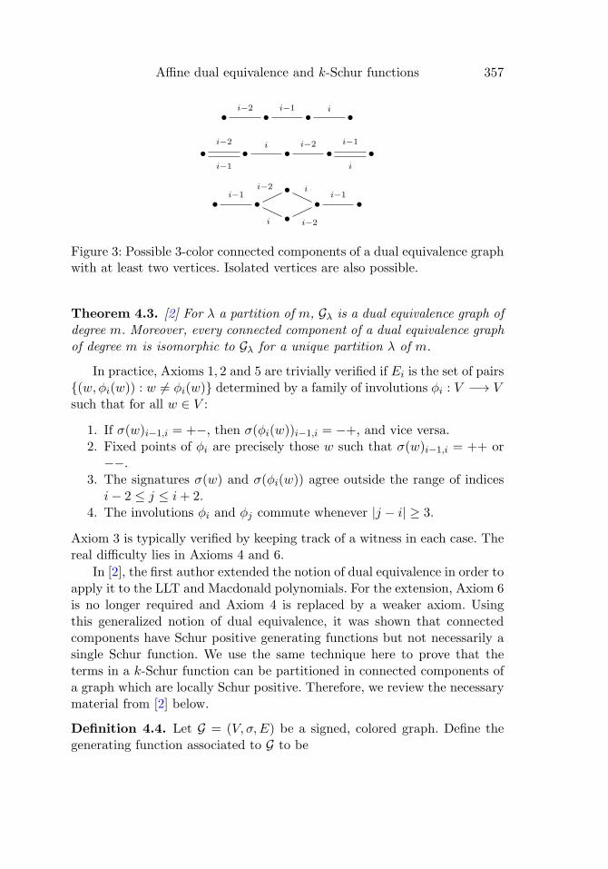
(ax4) For all 3 < i < m, every connected component of (V, σ,Ei−2 ∪Ei−1 ∪Ei) is either an isolated vertex or it is isomorphic to a graph in Fig-
ure 3 after the signature function is restricted to positions [i−2, i+1].
If m = 4, every connected component of (V, σ,E2 ∪ E3) is either an
isolated vertex or it is isomorphic to a connected component in an in-
duced subgraph of a graph in Figure 3 using only 2-edges and 3-edges
and restricting the signature function to positions [i− 1, i+ 1].
(ax5) Whenever |i− j| ≥ 3, {w, x} ∈ Ei and {x, y} ∈ Ej , there exists v ∈ V
such that {w, v} ∈ Ej and {v, y} ∈ Ei.
(ax6) Between any two vertices of a connected component of (V, σ,E2∪· · ·∪Ei), there exists a path containing at most one edge in Ei.
Comparing Figure 2 with Figure 3, the largest possible connected com-
ponents of (V, σ,Ei−2 ∪Ei−1 ∪Ei) are exactly the graphs for Gλ when λ is a
partition of 5. Taking this comparison to its ultimate conclusion yields the
following result.
Affine dual equivalence and k-Schur functions 357
Figure 3: Possible 3-color connected components of a dual equivalence graphwith at least two vertices. Isolated vertices are also possible.
Theorem 4.3. [2] For λ a partition of m, Gλ is a dual equivalence graph of
degree m. Moreover, every connected component of a dual equivalence graph
of degree m is isomorphic to Gλ for a unique partition λ of m.
In practice, Axioms 1, 2 and 5 are trivially verified if Ei is the set of pairs
{(w, φi(w)) : w = φi(w)} determined by a family of involutions φi : V −→ V
such that for all w ∈ V :
1. If σ(w)i−1,i = +−, then σ(φi(w))i−1,i = −+, and vice versa.
2. Fixed points of φi are precisely those w such that σ(w)i−1,i = ++ or
−−.
3. The signatures σ(w) and σ(φi(w)) agree outside the range of indices
i− 2 ≤ j ≤ i+ 2.
4. The involutions φi and φj commute whenever |j − i| ≥ 3.
Axiom 3 is typically verified by keeping track of a witness in each case. The
real difficulty lies in Axioms 4 and 6.
In [2], the first author extended the notion of dual equivalence in order to
apply it to the LLT and Macdonald polynomials. For the extension, Axiom 6
is no longer required and Axiom 4 is replaced by a weaker axiom. Using
this generalized notion of dual equivalence, it was shown that connected
components have Schur positive generating functions but not necessarily a
single Schur function. We use the same technique here to prove that the
terms in a k-Schur function can be partitioned in connected components of
a graph which are locally Schur positive. Therefore, we review the necessary
material from [2] below.
Definition 4.4. Let G = (V, σ,E) be a signed, colored graph. Define the
generating function associated to G to be
358 Sami H. Assaf and Sara C. Billey
FG(X) =∑v∈V
Qσ(v)(X).
Definition 4.5. A signed, colored graph G = (V, σ,E) of degree m is a D
graph if Axioms 1, 2, 3 and 5 (from Definition 4.2) hold for G. A D graph is
said to be locally Schur positive on h-colored edges, denoted LSPh, provided
for all 2 ≤ h < i < m:
(LSPh) Every connected component of (V, σ,Ei−h+1∪· · ·∪Ei) using h con-
secutive edge sets with signatures restricted to positions [i−h, i+1]
has a symmetric and Schur positive generating function.
For example, all of the graphs on Page 396 are locally Schur positive on
2-colored edges and 3-colored edges. Notice that any D graph satisfying Ax-
ioms 4 and 6 necessarily implies the graph is LSPh for all h by Theorem 4.3.
Observe that the signature function of a D graph can be recovered from
the edges plus a single sign in any one signature on any one vertex via the
axioms. Thus each graph in Figure 3 can be assigned signature functions in
exactly 2 ways which make them into a D graph. The third graph can only
be signed in one way up to isomorphism.
5. Poset on n-cores
In order to define an analog of dual equivalence for starred strong tableaux,
we must first understand saturated chains in the n-core poset. In this section,
we do this by exploiting the connection between n-cores and Sn using the
abacus model for partitions.
5.1. Covering relations
We can describe the n-core poset more directly using the abacus model for
cores from [14]. Consider the diagram of a partition λ, not necessarily an
n-core, lying in the N × N plane with infinite positive axes. Walk in unit
steps along the boundary of λ placing a bead (•) on each vertical step and
a spacer (◦) on each horizontal step. Then straighten the boundary to get a
doubly infinite rod with the main diagonal marked by a vertical line. This
gives the binary string uniquely representing λ when beads are replaced by
1’s and spacers by 0’s. For example, we construct the string for (4, 2) as
follows.

Affine dual equivalence and k-Schur functions 359
Define the content of a bead or spacer to be the content of the diagonalimmediately southeast. Indexing each bead or spacer by its content gives aninjective map from partitions to binary strings. The abacus associated to λis the binary string of λ with beads and spacers indexed by their content.
Remark 5.1. Given any doubly infinite binary string s such that si is a beadfor all i < l and si is a spacer for all i > r for some l, r, there is a uniquere-indexing of s making it an abacus associated to a (unique) partition.
Interchanging a bead on the abacus of μ with a spacer m places toits right corresponds to adding a ribbon of length m to μ, and similarlyinterchanging a bead with a spacer m positions to its left removes an m-ribbon from μ. In particular, if the moving bead lands in position s, thenthe head of the added ribbon will have content s− 1.
Divide the abacus into n rods, each containing all beads and spacers ofthe same residue. Removing an n-ribbon from the boundary of λ preciselycorresponds to moving a bead left along its rod. Therefore λ is an n-coreprecisely when each rod is an infinite string of beads followed by an infinitestring of spacers. Define the content of a rod to be the content of the beador spacer immediately to the right of the vertical line marking the maindiagonal. We will identify a rod by its content throughout the paper. Con-tinuing with the previous example, taking n = 3 gives the following abacusdecomposition of (4, 2), showing rods 1, 2 and 3.
Remark 5.2. Rotating the bottom row of the n-rod abacus for μ to thetop and shifting all beads in that row one column to the right will againrepresent the abacus for μ, but now shifted so that the rods have contents0, . . . , n−1 from top to bottom. Similarly, rotating the top row down to thebottom and shifting all beads left on that row gives the n-rod abacus for μwith contents 2, . . . , n + 1. Thus, the abacus can be represented by n rods

360 Sami H. Assaf and Sara C. Billey
of contents k, k + 1, k + 2, . . . , k + n− 1 for any integer k by scrolling up ordown.
Define the length of each rod of the n-rod abacus as follows. For i =1, 2, . . . , n, define the length of the rod with content i to be the number ofbeads on the rod with positive content minus the number of spacers on therod with nonpositive content (at most one of these numbers is nonzero).For example, the lengths of rods 1, 2, 3 for the 3-core (4, 2) are 2,−1,−1. Inline with Remark 5.2, define the length of the remaining rods by setting thelength of rod i − n equal to one plus the length of rod i. It is sometimesconvenient to rescale the lengths of the rods so that the rods 1, 2, . . . , nhave nonnegative length with at least one having length 0. For now, we areconcerned only with the relative lengths of the rods.
Affine permutations act on n-core partitions as discussed in Section 2.2.This action can be stated in terms of abaci as well. Recall we can representa partition by an infinite binary string. Since affine permutations are bijec-tions from Z to Z, we can apply such a bijection to any binary string. Ifthe binary string represents an n-core then any affine transposition appliedto the binary string will also represent an n-core. We leave it to the readerto verify this action is consistent with the action of simple affine transpo-sitions acting on n-cores described earlier. In particular, the action of anaffine transposition on an n-core can be thought of pictorially as exchangingtwo rods of its abacus and modifying all n-translates of these two rods ac-cordingly. The following observations, also noted in [17], follow easily fromthe abacus model.
Proposition 5.3. The following statements hold for an n-core μ and tr,s ∈Sn with r < s, r ≡ s:
1. The abacus for tr,sμ is obtained from the abacus for μ by swapping thelengths of the two rods with contents r and s. All rods with contentdistinct from r, s mod n have the same length in μ and tr,sμ.
2. In the n-core poset, tr,sμ > μ if and only if the rod of content r haslarger length than the rod of content s in μ.
3. An n-core λ covers μ if and only if λ = tp,qμ for some pair p < q, p ≡ qsuch that in the abacus for μ there is a bead at position p, a spacer atposition q, and no rod between p and q has length weakly between thelength of rod p and the length of rod q. Furthermore, the head and tailof one ribbon in λ/μ have contents q − 1 and p respectively.
Proof. The first statement follows form the action of an affine permutationon infinite binary strings. The second statement is immediate since moving

Affine dual equivalence and k-Schur functions 361
beads right adds ribbons and moving beads left removes ribbons. The thirdstatement also follows from this interpretation.
Proposition 5.3 is enough to describe precisely what λ/μ may look likewhen λ covers μ in the n-core poset. The condition on the lengths of therods that lie between the interchanging rods of the abacus implies that theconnected components of λ/μ are identical ribbons. By Remark 5.2, the tworods being exchanged must have distinct residues and no rod between themmay have the same residue as either of them. The contents across which thebeads move determine the contents contained in the ribbons, and the factthat both rods are beads followed by spacers ensures that the ribbons lieon consecutive residues. These observations reprove the following statementdue to Lam, Lapointe, Morse and Shimozono.
Corollary 5.4. [17, Prop. 9.5] Let μ be an n-core and tr,s an affine trans-position such that tr,sμ covers μ in the n-core poset. Then 0 < s − r < nand the connected components of tr,sμ/μ are identical shape ribbons with cellresidues from r mod n to s− 1 mod n. Moreover, if rod r has k > 0 morebeads than rod s, then tr,sμ/μ has exactly k identical ribbons. If the headof the first ribbon lies in a cell with content c, then the head of the otherribbons have content c+ n, c+ 2n, . . . , c+ (k − 1)n.
By Corollary 5.4, for a strong tableau S of shape λ, call the connectedcomponents of λi/λi−1 the i-ribbons of S. Recall from Section 3.2 that astarred strong tableau consists of a strong tableau plus a choice of i-ribbonfor each i present in S. We use the next definition and corollary to relatethe starred strong tableaux to saturated chains labeled by certain sequencesof transpositions.
Definition 5.5. Let μ ⊂ λ be n-cores, and let T (λ/μ, n) be the set of alltransposition sequences (tr1s1 → tr2s2 → · · · → trmsm) such that
1. the product trmsm · · · tr2s2tr1s1μ = λ as elements of Sn/Sn;2. for each 1 ≤ i ≤ m, we have 0 < si − ri < n;3. for each 0 ≤ i < m, the abacus for μ(i) = trisi · · · tr2s2tr1s1μ contains
a bead at position ri+1, a spacer at position si+1, and every rod withcontent between ri+1 and si+1 has length strictly smaller than boththe length of rod ri+1 and the length of rod si+1 or strictly larger thanboth.
By Proposition 5.3, condition (3) above implies μ = μ(0) < μ(1) < · · · <μ(m) = λ forms a saturated chain in the n-core poset. The following is aconsequence of Proposition 5.3 and Corollary 5.4.

362 Sami H. Assaf and Sara C. Billey
Corollary 5.6. Let μ ⊂ λ be n-cores. There exists a bijection from skewstarred strong tableaux S∗ ∈ SST∗(λ/μ, n) to T (λ/μ, n) given by mapping
S∗ �→ (tr1s1 → tr2s2 → · · · → trmsm)
where si − 1 and ri are the contents of the head and tail of the i-ribboncontaining i∗ in S∗.
For example, this bijection maps
.
5.2. Intervals of length two
As motivation, recall that an elementary dual equivalence on standardtableaux may be defined in terms of interval exchanges in Young’s lattice.Though the induced poset on n-cores in not as nice as Young’s lattice,Bjorner and Brenti [5] showed that any interval of length two is either achain or isomorphic to B2.
Definition 5.7. Let S = (∅ = μ0 ⊂ μ1 ⊂ · · · ⊂ μm) be a saturated chainin the n-core poset such that the interval [μi−1, μi+1] is not a chain for0 < i < m. The i-interval swap on S, denoted swapi,i+1(S) = swapi+1,i(S),replaces μi with the unique other n-core at rank i in [μi−1, μi+1].
For example, from Figure 1 we see that a 2-interval swap on the chain
results in the chain
.
In terms of the strong tableaux, the same 2-interval swap gives
.(5.1)
Affine dual equivalence and k-Schur functions 363
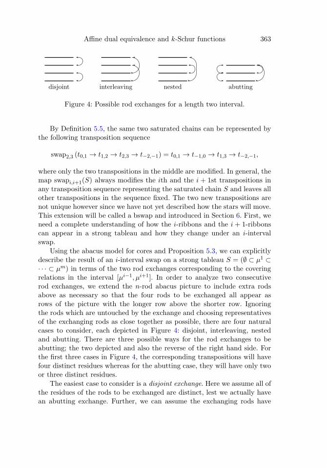
Figure 4: Possible rod exchanges for a length two interval.
By Definition 5.5, the same two saturated chains can be represented bythe following transposition sequence
swap2,3 (t0,1 → t1,2 → t2,3 → t−2,−1) = t0,1 → t−1,0 → t1,3 → t−2,−1,
where only the two transpositions in the middle are modified. In general, themap swapi,i+1(S) always modifies the ith and the i + 1st transpositions inany transposition sequence representing the saturated chain S and leaves allother transpositions in the sequence fixed. The two new transpositions arenot unique however since we have not yet described how the stars will move.This extension will be called a bswap and introduced in Section 6. First, weneed a complete understanding of how the i-ribbons and the i + 1-ribbonscan appear in a strong tableau and how they change under an i-intervalswap.
Using the abacus model for cores and Proposition 5.3, we can explicitlydescribe the result of an i-interval swap on a strong tableau S = (∅ ⊂ μ1 ⊂· · · ⊂ μm) in terms of the two rod exchanges corresponding to the coveringrelations in the interval [μi−1, μi+1]. In order to analyze two consecutiverod exchanges, we extend the n-rod abacus picture to include extra rodsabove as necessary so that the four rods to be exchanged all appear asrows of the picture with the longer row above the shorter row. Ignoringthe rods which are untouched by the exchange and choosing representativesof the exchanging rods as close together as possible, there are four naturalcases to consider, each depicted in Figure 4: disjoint, interleaving, nestedand abutting. There are three possible ways for the rod exchanges to beabutting; the two depicted and also the reverse of the right hand side. Forthe first three cases in Figure 4, the corresponding transpositions will havefour distinct residues whereas for the abutting case, they will have only twoor three distinct residues.
The easiest case to consider is a disjoint exchange. Here we assume all ofthe residues of the rods to be exchanged are distinct, lest we actually havean abutting exchange. Further, we can assume the exchanging rods have

364 Sami H. Assaf and Sara C. Billey
contents a < b < c < d with n > d − a > 0 since the rods are as closetogether as possible. The two exchanges in this case clearly commute, andtaking either first raises the rank by exactly one by Corollary 5.4. In thestrong tableau, such an i-interval swap will happen precisely when the cellsof the i-ribbons and (i + 1)-ribbons have no residues in common, and theeffect of the swap will be to exchange all i’s for i+ 1’s and conversely.
The case of an interleaving exchange is only slightly more interesting,though the conclusion of this case is noteworthy. Labeling the residues ofthe exchanging rods a < b < c < d from top to bottom, again we assumeall four residues to be distinct lest we be pulled into the abutting case. Theassumption that these two exchanges each increase the rank in the posetforces rod a longer than rod c and similarly rod b longer than rod d byProposition 5.3. Suppose μi−1 ⊂ ta,cμ
i−1 = μi ⊂ tb,dta,cμi−1 = μi+1; the
other case is similarly resolved. By Proposition 5.3, this means the length ofrod b does not lie between the lengths of rods a and c and that the lengthof rod a does not lie between the lengths of rods b and d. Recall, we chosea picture for the abacus so that the length of rod b is larger than the lengthof rod d and the length of rod a is longer than the length of rod c. Thesestatements together imply that the lengths of rods a and c do not interleavethe lengths of rods b and d, and so the transpositions taken in the other ordereach raise the rank by exactly one, thus μi−1 ⊂ tb,dμ
i−1 ⊂ ta,ctb,dμi−1 = μi+1
is a valid strong tableau. In this new strong tableau, the contents of the i-ribbons and i + 1-ribbons will not overlap, though the residues will. It isalso important to note that the i-ribbons and i+1-ribbons will not have thesame residues for their heads or tails. In this case, the i-interval swap againsimply exchanges all i’s for i + 1’s and conversely. We summarize the keyobservation in this case as follows.
Proposition 5.8. An i-ribbon and an i+ 1-ribbon in a strong tableau haveoverlapping contents if and only if the contents of one ribbon are strictlycontained in the contents of the other. Furthermore, the contents of the headand tail of the longer ribbon do not occur among the contents of the shorterribbon.
More generally, we say two ribbons are nested if the second condition ofProposition 5.8 holds. We also say two ribbons R1 and R2 are independentif R1 ∪R2 has two connected components as a skew shape.
In the case of a nested exchange, again label the rod contents a < b <c < d from top to bottom. We can assume d− a < n by Corollary 5.4. Herethe two corresponding transpositions commute, and each will raise the rankby exactly one. The interesting feature of this case lies in way the nested

Affine dual equivalence and k-Schur functions 365
Figure 5: A nested exchange is show on two 4-core skew strong tableaux.
ribbons can appear in the corresponding strong tableaux. See Figure 5 for
example.
By Proposition 5.3, neither the length of rod b nor the length of rod c
may lie between the lengths of rods a and d. If both rod b and rod c are
longer than rod a or both shorter than rod d (necessarily rod a is longer
than rod d), then the i-ribbons and i + 1-ribbons will have no contents in
common, though the residues of one ribbon will be strictly contained within
the residues of the other. Furthermore, both the heads and tails of the i-
ribbons and i+ 1-ribbons have distinct residues.
On the other hand, if rod b is longer than rod a and rod c is shorter
than rod d (necessarily rod b is longer than rod c), then the content of every
instance of the longer ribbon (corresponding to ta,d) overlaps the content of
a shorter ribbon (corresponding to tb,c) and there must be an instance of the
shorter ribbon containing a cell of content b− 1 which occurs independently
from all of the longer ribbons. An i-interval swap changes all entries in all of
the shorter ribbons that appear independently of the longer ribbons and all
entries of the longer ribbons that are not on the same content as a shorter
ribbon.
For example, we can apply a nested exchange to the 4-core partition
(4, 1, 1, 1) encoded as an abacus with 4 rods, numbered 1, 2, 3, 4, with lengths
(−1, 0, 0, 1). The nested exchange is more clear if we instead consider the
same abacus but with rods numbered −1, 0, 1, 2 by scrolling (−1, 0, 0, 1) back
two steps to (1, 2,−1, 0) via Remark 5.2. Now, we are in the case where
a = −1, b = 0, c = 1, d = 2, rod a has length 1, rod b has length 2, rod c has
length −1, and rod d has length 0. These rod lengths satisfy the conditions of
a nested exchange of the second type described above. Applying the nested
exchange corresponding to the two commuting transpositions t−1,2t0,1 results
in rod lengths (0,−1, 2, 1) which encode the 4-core partition (5, 3, 3, 1, 1). In
terms of strong tableaux, the two transposition sequences t−1,2 → t0,1 and
t0,1 → t−1,2 applied to μ = (4, 1, 1, 1) are related by swap7,8 as shown below.
This discussion proves the following lemma.

366 Sami H. Assaf and Sara C. Billey
Lemma 5.9. If an i-ribbon and an i+ 1-ribbon are nested, then
1. At least two copies of the shorter ribbon occur independently from thelonger ribbon, with at least one on either side of the consecutive se-quence of copies of the longer ribbon.
2. Every copy of the longer ribbon nests a copy of the shorter ribbon.3. Both the heads and tails of the i-ribbons and i+1-ribbons have distinct
residues.4. An i-interval swap is possible.
The final case of an abutting exchange will involve exactly three distinctindices on the transpositions, though possibly only two distinct residues.Let μ be an n-core partition represented as an n rod abacus with threehighlighted rods among them with contents a < b < c from top to bottomon which we can apply an abutting exchange. Suppose that the three residuesof a, b, c are all distinct. This is necessarily the case for the right hand side ofFigure 4. Say the two exchanges correspond with the transposition sequence(ta,c → ta,b). Then by Proposition 5.3, we know rod a is strictly longer thanrod c. Similarly, since we can apply tab to the partition tacμ, we also knowthat rod c is longer than rod b, so the three rod lengths are totally ordered.We note that tb,cta,b = ta,bta,c so this equation along with the total order onthe lengths of the rods ensures that an interval swap is possible. The newtransposition sequence after applying this interval swap would be (ta,b →tb,c) which corresponds with the left hand side of the abutting exchangepictured in Figure 4. If the two exchanges correspond with the transpositionsequence (ta,b → ta,c), examining the required rod length inequalities againwe see that (tb,c → ta,b) is a valid transposition sequence on the same rank2 interval. This again corresponds with the left hand side of the abuttingexchange pictured in Figure 4. If the right hand side of Figure 4 is turnedupside down, a similar analysis holds. Furthermore, the interval swaps forman involution on the two chains in any interval isomorphic to B2 so we havecovered all possible cases of an abutting exchange in the form of the lefthand side of the abutting picture of Figure 4 as well. Hence in all cases ofan abutting exchange with three distinct residues, there exists an intervalswap determined above.
Assuming that [μi−1, μi+1] is isomorphic to B2, one way to recognize ifan abutting exchange is required for swapi,i+1(S) is that an i-ribbon and ani+1-ribbon together form a ribbon shape. In this case, we will say these tworibbons abut each other. From the transpositions pictured in the abuttingcase of Figure 4 and Corollary 5.4, we observe that the sum of the lengthsof an i-ribbon and an i + 1-ribbon is necessarily less than n and exactly

Affine dual equivalence and k-Schur functions 367
one of the two ribbon types occurs without abutting a copy of the other. Inthis instance, the i-interval swap will change all entries of the non-abuttingribbons and all entries in their n-translates. For example, the 2-ribbon abutsa 3-ribbon in the strong tableau on the left in (5.1).
The other way to recognize if an abutting exchange is required forswapi,i+1(S) is that, among the i, i+1-ribbons, one ribbon is strictly longerthan the other and the longer ribbon contains an n-translate of the shorterand the heads or tails of the two ribbons have the same residue dependingon if the shared rod is a or c. See for example, the 2-ribbon and 3-ribbon inthe strong tableau on the right in (5.1). Here an interval swap will change allentries of the shorter ribbons and all entries of the longer ribbons that arenot part of an n-translate of the shorter. This case is also recovered from theleft hand side of Figure 4 when the lengths of the three rods are all distinct;we omit details as the case is completely parallel.
Following the details of the abutting exchange case carefully, we havethe following.
Proposition 5.10. Suppose swapi,i+1(S) is obtained from S by an abuttingexchange. Assume the corresponding transpositions are indexed by 3 distinctresidues mod n. Then either
• No i-ribbon abuts any i + 1-ribbon, but one of these ribbons strictlycontains an n-translate of the other with a shared head or tail occurringon a consecutive residue.
• OR, all instances of one ribbon type abut the other while the other willalso have at least one components which is non-abutting and the sumof the length of an i-ribbon and an i + 1-ribbon is at most n − 1. Inthis case, if an i+ 1-ribbon abuts an i-ribbon from the north, then thenon-abutting ribbons lie always southeast of the abutting ribbons, andif an i-ribbon abuts an i+1-ribbon from the west, then the non-abuttingribbons lie always northwest of the abutting ribbons.
Finally, consider an abutting exchange as in the left hand side of theabutting case in Figure 4. If the three rod lengths are distinct and the threeresidues are distinct, then the exchange is covered by Prop 5.10. In eachof the remaining cases, we claim the interval [μi−1, μi+1] is a chain so ani-interval swap is not possible.
Proposition 5.11. Let S = (∅ = μ0 ⊂ μ1 ⊂ · · · ⊂ μm) be a saturated chainin the n-core poset. Then the interval between μi−1 and μi+1 in the n-coreposet is a chain if and only if each i-ribbon abuts an i + 1-ribbon and eachi + 1-ribbon abuts an i-ribbon. Moreover, the length of an i-ribbon plus the
368 Sami H. Assaf and Sara C. Billey
length of a i+1-ribbon is less than or equal to n, with equality if and only ifμi+1/μi−1 is a single connected ribbon shaped component starting and endingwith i+ 1-ribbons.
Proof. Assume [μi−1, μi+1] is a chain. Then by the previous analysis of twoconsecutive rod exchange cases examined in this section above, one can showthat a length 2 chain corresponds with a transposition sequence of the formtb,c → ta,b with a < b < c or a > b > c.
Assume a and c have different residues (both necessarily have distinctresidues from b). In this case, ta,btb,c = ta,cta,b, and by Proposition 5.3 wecan assume 0 < c− a < n. Thus, we see from the n-rod abacus model thatthe skew shape μi+1/μi−1 is the union of a positive number of n-translatesof a single ribbon shape of length less than n and none of these ribbonsoverlap in content. More precisely, i-ribbons and i+1-ribbons always occurin connected pairs and the sum of their lengths is strictly less than n. Forexample, the 3-ribbons and 4-ribbons in the first strong tableau in (3.1)have this property, and interpreting this strong tableau as a saturated chainone can see the corresponding chain property from the poset in Figure 1 onranks 2 to 4.
If, on the other hand, a and c have the same residue, then we can as-sume c = a+n by choosing to label the exchanging rods as close together aspossible. Hence, the length of the ribbons corresponding to ta,b and those cor-responding to tb,a+n necessarily add to n so μi+1/μi−1 is a single connectedribbon shaped component. Furthermore, recall that rod c is one shorterthan the length of rod a by Remark 5.2 and the fact c = a + n. If rod bis shorter than rod a, then the chain corresponds with the transpositionsequence ta,b → tb,c, otherwise the transpositions happen in the reverse or-der. In either case, by considering how ribbons are created using the abacusmodel and Proposition 5.3, we observe that the ribbon μi+1/μi−1 is tiledby an alternating sequence of i-ribbons and i+ 1-ribbons and it begins andends with an i+1-ribbon. The last tableau in (3.1) has this property on the3-ribbons and 4-ribbons, as does the strong tableau underlying both picturesin Figure 10 on the 2, 3-ribbon and the 1, 2-ribbon.
To prove the reverse direction, assume each i-ribbon abuts an i + 1-ribbon and conversely. Then by Corollary 5.4 we can infer that the chainμi−1 ⊂ μi ⊂ μi+1 corresponds to an abutting exchange. If all three contentsof the exchanging rods have distinct residues, then either [μi−1, μi+1] is achain or we would find a contradiction to the second case of Proposition 5.10.
If there are only two distinct indices among the exchanging rods thenthe relative lengths of these rods determine the only possible exchange se-quence taking μi−1 to μi+1 by Proposition 5.3. Thus, [μi−1, μi+1] is again achain.
Affine dual equivalence and k-Schur functions 369
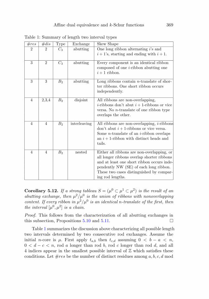
Table 1: Summary of length two interval types
#res #dis Type Exchange Skew Shape2 2 C3 abutting One long ribbon alternating i’s and
i+ 1’s, starting and ending with i+ 1.
3 2 C3 abutting Every component is an identical ribboncomposed of one i-ribbon abutting onei+ 1 ribbon.
3 3 B2 abutting Long ribbons contain n-translate of shor-ter ribbons. One short ribbon occursindependently.
4 2,3,4 B2 disjoint All ribbons are non-overlapping,i-ribbons don’t abut i+ 1-ribbons or viceversa. No n-translate of one ribbon typeoverlaps the other.
4 4 B2 interleaving All ribbons are non-overlapping, i-ribbonsdon’t abut i+ 1-ribbons or vice versa.Some n-translate of an i-ribbon overlapsan i+ 1-ribbon with distinct heads andtails.
4 4 B2 nested Either all ribbons are non-overlapping, orall longer ribbons overlap shorter ribbonsand at least one short ribbon occurs inde-pendently NW (SE) of each long ribbon.These two cases distinguished by compar-ing rod lengths.
Corollary 5.12. If a strong tableau S = (μ0 ⊂ μ1 ⊂ μ2) is the result of anabutting exchange, then μ2/μ0 is the union of ribbons with nonoverlappingcontent. If every ribbon in μ2/μ0 is an identical n-translate of the first, thenthe interval [μ0, μ2] is a chain.
Proof. This follows from the characterization of all abutting exchanges inthis subsection, Propositions 5.10 and 5.11.
Table 1 summarizes the discussion above characterizing all possible lengthtwo intervals determined by two consecutive rod exchanges. Assume theinitial n-core is μ. First apply ta,b then tc,d assuming 0 < b − a < n,0 < d − c < n, rod a longer than rod b, rod c longer than rod d, and all4 indices appear in the smallest possible interval of Z which satisfies theseconditions. Let #res be the number of distinct residues among a, b, c, d mod

370 Sami H. Assaf and Sara C. Billey
n. Let #dis be the number of distinct rod lengths among rods a, b, c, d inμ. The interval [μ, tcdtabμ] is either isomorphic to B2 or the chain C3 with3 elements. The two interval types are distinguished by considering #resand #dis or equivalently by considering the skew shape as partitions oftcdtabμ/μ.
6. Affine dual equivalence
We now have all the ingredients to construct an analog of dual equivalencefor starred strong tableaux, which we call affine dual equivalence. Though ourequivalence relation will not share all of the properties of dual equivalenceon tableaux, we will go on in Section 7 to construct a signed colored graphfrom our elementary equivalence relations that we show to be a D graph.
While the elementary equivalence relations will have a somewhat com-plicated description, there are essentially only two cases: one that preciselymirrors dual equivalence, and another that is a close approximation whenthe former is not applicable. Remarkably, the relations also preserve the spinstatistic on starred strong tableaux.
6.1. Elementary equivalences
In this subsection, we describe a family of involutions ϕi on all starredstrong tableaux of a given shape that will define the elementary affine dualequivalence on i−1, i, i+1. Recall that a starred strong tableau S∗ of shapeλ can be represented by a strong tableau S = (∅ ⊂ λ(1) ⊂ λ(2) ⊂ · · · ⊂ λ(m))with λ(m) = λ and a vector c∗ = (c1, c2, . . . , cm) where ci is the content ofthe cell of S∗ containing i∗. In this case, we will say the rank of S∗ is m.
Definition 6.1. Let S∗ = (S, c∗) be a starred strong tableau of rank m. Fix1 < i < m. Consider the locations of (i−1)∗, i∗, (i+1)∗ in S∗. The i-witness,or simply the witness when i is fixed, is chosen among {i − 1, i, i + 1} asfollows.
1. If ci−1 = ci+1, then ci−1, ci, ci+1 are all distinct since consecutive rib-bons cannot have heads or tails of the same content by the analysis inSection 5.2. In this case, the witness is the index of the median of theset {ci−1, ci, ci+1}.
2. If ci−1 = ci+1, then we have three cases to consider.
(a) If the (i − 1)-ribbons and (i + 1)-ribbons have the same length,then i+ 1 is the witness.

Affine dual equivalence and k-Schur functions 371
Figure 6: The witnesses from left to right are 3,1,3 demonstrating parts 2(a),2(b) and 2(c) respectively in Definition 6.1.
(b) If the (i − 1)-ribbons and (i + 1)-ribbons have different lengthsand ci−1 > ci, then the witness is the letter indexing the longerribbons among the (i− 1)-ribbons and the (i+ 1)-ribbons.
(c) If the (i − 1)-ribbons and (i + 1)-ribbons have different lengthsand ci−1 < ci, then the witness is the letter indexing the shorterribbons among the (i− 1)-ribbons and the (i+ 1)-ribbons.
In Figure 6, we give three examples where the witness is computed usingPart (2) of Definition 6.1. Note, i − 1, i, i + 1 have been replaced by 1, 2, 3in the examples to emphasize that we only care about 3 consecutive valueswhen computing the witness. The exact value of i is irrelevant.
Note that when S∗ is a Young tableau, the contents of the unique cellscontaining i − 1, i and i + 1 must all be distinct, ensuring that the witnessis always the index of the median of the set {ci−1, ci, ci+1}.
Next we define the involution ϕi on starred strong tableaux that willserve as a model for dual equivalence. Intuitively, if i and j are witnessedby h in S∗, then an elementary dual equivalence move should be based onthe map swapi,j where {h, j} = {i−1, i+1}. This would be straightforwardbut for the difficulty of defining how the stars should behave under suchan action. We obtained these rules experimentally guided by the principlethat the stars should move as little as possible while preserving the spinstatistic, always remaining in the same connected component of the unionof cells in S∗ containing i− 1, i, i+ 1 but necessarily switching which letterthey adorn whenever i = h. This will be the action of ϕi whenever such amove is possible without changing the witness. However, if the interval isa chain and the starred letters both lie in the same connected component,then neither an interval swap nor a star swap is possible. We overcome thischallenge by exchanging saturated chains of length three.

372 Sami H. Assaf and Sara C. Billey
Definition 6.2. Fix a starred strong tableau S∗ = (S, c∗) of rank m with1 < i < m. Let h be the i-witness for S∗. If h = i, then let j be defined by{i − 1, i + 1} = {j, h}. Let Sq be the union of all q-ribbons and let Sq∗ bethe connected component of Sq containing q∗ for 1 ≤ q ≤ m. We will say Sq
nests Sp∗ if the content of every cell of Sp∗ is also the content of a cell inSq but no head or tail of a ribbon in Sq has the same content as the heador tail of Sp∗ . Similarly, a connected skew shape A nests another connectedskew shape B provided the content of every cell of B is the content of somecell of A, but the largest and smallest contents of cells in A are not thecontents of any cells in B. Let bq be the content of the ribbon tail for Sq∗ .We will say Si and Sj are not abutting if bi, bj , (ci+1), (cj +1) have distinctresidues, otherwise Si and Sj are abutting. Let Bi and Bj be the connectedcomponents of Si ∪ Sj containing i∗ and j∗, respectively.
Then ϕi(S∗) is defined by the first case that applies below. N.B. The
order matters.
(6.1)
ϕi(S∗) =
⎧⎪⎪⎪⎪⎪⎪⎪⎪⎪⎪⎪⎪⎪⎪⎪⎪⎪⎪⎪⎪⎪⎨⎪⎪⎪⎪⎪⎪⎪⎪⎪⎪⎪⎪⎪⎪⎪⎪⎪⎪⎪⎪⎪⎩
S∗ if i = h,
bswapi,j(S∗) if Si and Sj are not abutting,
bswapi,j(S∗) if Bi and Bj have different shapes
and neither nests Sh∗ ,
snakehi,j(S∗) if bh ≡ bj and ch ≡ cj ,
bswapi,jbswapi,h(S∗) if Si or Sj nests Sh∗ ,
doublehi,j(S∗) if Bi or Bj nests Sh∗ ,
stari,j(S∗) if Bi = Bj but they have
the same shape.
Here the map ϕi depends on four types of ribbon swaps: basic swap,snake swap, double swap, and star swap. Each of these maps are definedbelow with an example on starred strong tableaux. One can already observethat for every starred strong tableau of rank m at least one of the conditionsfor ϕi must be met whenever 1 < i < m.
Note that the ribbon swaps will only be well-defined under certain cir-cumstances. We prove, in a series of lemmas following the definitions, thatthe circumstances where a ribbon swap is applied in (6.1) will be preciselythe circumstances when the ribbon swap is well-defined and ϕi acts as an

Affine dual equivalence and k-Schur functions 373
involution. The lemmas then immediately imply Theorem 6.12, which saysthat ϕi : SST
∗(λ/μ, n) → SST∗(λ/μ, n) is a well-defined involution. To showϕi is an involution, it is essential to keep track of the witness h∗. We advisethe reader to pay careful attention to the witness in each of the ribbon swapdefinitions and examples.
The basic swap, denoted bswapi,j(S∗), is the result of an interval swap
on S and interchanging the blocks containing i∗ and j∗
bswapi,j(S∗) = (swapi,j(S), c
∗(Bi ↔ Bj)).
For example, if n = 4 and i = 4 then ϕ4 = bswap4,5 interchanges
.(6.2)
In the left tableau, B4 is the cell of content 3 filled by 4∗ and B5 is the setof cells with contents {−1,−2} filled by 4, 5∗. In the right tableau B5 is thecell of content 3 and B4 is the set of cells with contents {−1,−2}. Note,the star in the {−1,−2} block must move when applying the map in eitherdirection so as to return a valid starred strong tableau with a star at thehead of an i-ribbon and a j-ribbon.
A description of the operation c∗(Bi ↔ Bj) is given specifically as fol-lows. Let dp = cp +1 for each p so that the p-ribbons in S∗ correspond withapplying the transposition tbp,dp
. Let rp = dp−bp be the length of a p-ribbonin S∗. Let εp be the unit vector with a 1 in the p-th position. Assume p < q,then define
(6.3)
flopq,p(c∗) = flopp,q(c
∗) =
⎧⎪⎪⎪⎪⎪⎪⎨⎪⎪⎪⎪⎪⎪⎩
tp,q(c∗)− rp · εp if dp ≡ dq and |Bp| < |Bq|,
tp,q(c∗)− rq · εq if dp ≡ dq and |Bp| > |Bq|,
tp,q(c∗) + rq · εq if bq ≡ dp and |Bp| > |Bq|,
tp,q(c∗) + rp · εp if bp ≡ dq and |Bp| < |Bq|,
tp,q(c∗) otherwise.
Therefore, formally we define
bswapi,j(S∗) = (swapi,j(S), flopi,j(c
∗)).
We prove bswapi,j(S∗) is always a valid starred strong tableau in Lemmas 6.5
and 6.6.

374 Sami H. Assaf and Sara C. Billey
Remark 6.3. Observe that flopi,j(c∗) = ti,j(c
∗ if and only if Si and Sj are
not abutting. It might seem easier to remove this case from the definition
of a flopi,j , however, that would add extra cases later when we discuss the
case Si or Sj nests Sh∗ .
Remark 6.4. Note that when S∗ is a Young tableau, it is impossible for the
cell containing i to abut the cell containing j when h = i is the witness.
Therefore the required ribbon swap in this case will always be ϕi(S∗) =
bswapi,j(S∗) = (swapi,j(S), ti,j(c
∗)). Hence ϕi reduces to the usual elemen-
tary dual equivalence relation on Young tableaux.
The snake swap, denoted snakehi,j(S∗), is the result of moving the stars
on all three ribbons i−1, i, i+1 while keeping the underlying strong tableau
fixed. If i− 1 is the witness, the moves are based on the permutation 231 =
t12t23; if i+1 is the witness, the moves are based on the permutation 312 =
t23t12. Either way, j will become the i-witness of snakehi,j(S∗). Assuming h
is the witness, then
(6.4)
snakehi,j(S∗) =
{(S, ti,jti,h(c
∗)− rj · εi + rh · εh) if (cj < ci) xor (i < j),
(S, ti,jti,h(c∗) + ri · εi − ri · εh) otherwise.
We will show in the proof of Theorem 6.12 that snakehi,j is only applied
when Si∪Sj and Si∪Sh are both single connected ribbons so [λ(i−2), λ(i+1)]
is a chain by Proposition 5.11. When h = i + 1, the stars move away from
the diagonal of content ch along these ribbons and when h = i− 1 the stars
move in toward the diagonal of content ch along these ribbons. The star
on the witness toggles between h and j by sliding along the diagonal with
content ch. For example, if n = 2 and i = 3, then ϕ3 = snake43,2 maps
.
The inverse map is given by snake23,4 applied to the tableau on the right.
The double swap, denoted doublehi,j(S∗), is the result of two interval
swaps on S and another “almost permutation” of the three relevant indices
in the content vector. Precisely,
doublehi,j(S∗) =
{(swapi,jswapi,h(S), ti,jti,h(c
∗) + rh · εh)
if bh ≡ bj ,(swapi,jswapi,h(S), ti,jti,h(c
∗)− rh · εi)
if ch ≡ cj .

Affine dual equivalence and k-Schur functions 375
Since doublehi,j is only applied when Bi or Bj nests Sh∗ but neither Si orSj nests Sh∗ , we can conclude that the nesting block is a ribbon and thatSj contains a cell with the same content as either the head or tail of Sh∗
by considering all possible rank 2 abutting rod exchanges. Thus, when itsapplied either bh ≡ bj or ch ≡ cj . For example, if n = 3 and i = 4, then ϕ4
interchanges the following tableaux via double swaps:
.
The star swap, denoted stari,j(S∗), is the result of moving the star on i∗
to the adjacent j-ribbon and vice versa while keeping the underlying strongtableau fixed. To be precise, if Bi and Bj are distinct and both Bi and Bj
contain both an i and j-ribbon, then both blocks have the same shape byProposition 5.10 and Proposition 5.11. Say f is the offset of the contents ofBj from Bi, so ci + f is the content of the head of the i-ribbon in Bj andcj − f is the content of the head of the j-ribbon in Bi. Then
stari,j(S∗) = (S, c∗ + f · εi − f · εj).
For example, if n = 4 and i = 6, then ϕ6 = star6,7 interchanges
.
6.2. A well-defined involution
Given the complicated definition of the affine dual equivalence relations, itis not obvious that ϕi is well-defined, much less that it is an involution.Our next task is to establish these two facts. In the course of doing so, weprovide many more examples of the action of ϕi, though in the interest ofspace only the relevant cells in the strong tableaux are shown. Since theargument involves many details, it may comfort the reader to know thatthe conclusion of this subsection Theorem 6.12 has also been verified bycomputer using the techniques from Section 7.
For each of the following lemmas and proofs, we assume all of the nota-tion from Definition 6.2. In particular, assume 1 < i < m, and let S∗ be astarred strong tableau with i-ribbons in the skew shape Si, j-ribbons in the

376 Sami H. Assaf and Sara C. Billey
shape Sj , the block Bi is the connected component of Si ∪ Sj containing i∗,etc. We can assume i = h throughout the proofs, otherwise ϕi(S
∗) = S∗ by
definition.
Lemma 6.5. Assume i = h and that Si and Sj are not abutting. Then
bswapi,j(S∗) is a valid starred strong tableau that satisfies the same assump-
tions and bswapi,jbswapi,j(S∗) = S∗.
Proof. In this case, a swapi,j(S) is well defined and bi, bj , di, dj are all dis-
tinct mod n by the classification of rod exchanges for rank 2 intervalsin Section 5.2. Unless Si and Sj come from an interleaving rod exchange
with some i-ribbon nested in an i + 1-ribbon or vice versa, the intervalswap will simultaneously change all i’s to j’s and conversely. Therefore
ϕi(S∗) = bswapi,j(S
∗) = (swapi,j(S), ti,j(c∗)) is a well-defined starred strong
tableau with stars in the original cells in S∗, though now adorning the op-posite letter among {i, j} from before. When Si and Sj come from an inter-
leaving rod exchange with some i-ribbon nested in an i + 1-ribbon or viceversa, then the interval swap will change all entries in the shorter ribbon
appearing independently as well as entries in the longer ribbon not on thesame content as a shorter ribbon. In particular, the shape of the blocks Bi
and Bj remains unchanged. Therefore bswapi,j(S∗) is again a valid starred
strong tableau. In this case, the star adorning the longer ribbon remains inplace, and the star adorning the shorter ribbon remains if the shorter ribbon
is not nested in a longer, otherwise it slides one position along the diagonal;see Figure 7 for an example.
Consequently, in order to show ϕi is an involution in this case, it remainsonly to show that h remains the witness after applying bswapi,j . Since the
effect on the content vector is merely to interchange ci and cj , the resultfollows provided ch = cj . However, the contrary case forces an i-ribbon to
abut both the i−1-ribbon and i+1-ribbon with heads on content ci−1 = ci+1.This would force the tail of the i-ribbons to be on the next diagonal in orderto create a valid skew shape, contradicting the assumption that Si and Sj
are not abutting. Hence, bswapi,j is an involution in this case.
Henceforth, we can assume that Si and Sj are abutting, and thus both
Bi and Bj must have ribbon shape by Corollary 5.12.
Lemma 6.6. Assume i = h and that Si and Sj are abutting. Further assume
that Bi and Bj have different ribbon shapes but neither nests Sh∗. Then T ∗ =bswapi,j(S
∗) is a starred strong tableau that satisfies the same assumptionsand bswapi,j(T
∗) = S∗.

Affine dual equivalence and k-Schur functions 377
Figure 7: The action of ϕi when Si and Sj are nested, hence not abutting.
Figure 8: The action of ϕi when Si ∪ Sj is abutting and Sh is not nested.
Proof. Since Bi and Bj have different shapes, the map swapi,j will togglebetween each block containing only one letter and exactly one of these blockscontaining both letters as shown in Figure 8. By Proposition 5.10 one candeduce how the stars move in the blocks Bi and Bj in order to adorn theother letter. These moves are summarized in the function flopi,j(c
∗). Hence,T ∗ = ϕi(S
∗) = bswapi,j(S∗) is a well defined starred strong tableau. Fur-
thermore, by inspection we have that bswapi,j(T∗) = S∗. Thus, ϕi(S
∗) is aninvolution provided h is also the i-witness of T ∗.
Observe that the only way for the witness to change is if h∗ lies on a di-agonal within a block containing both i’s and j’s, and h∗ lies weakly betweentheir respective heads. Let I and J be the abutting i-ribbon and j-ribbon inthe block overlapping h∗. By Proposition 5.8, consecutive ribbons may nothave partially overlapping contents. Therefore if an h-ribbon has contentoverlapping an i-ribbon, one of the two must be nested. By assumption, Sh∗
is not nested inside either Bi or Bj , hence is not nested in I. On the otherhand, if h-ribbons nest i-ribbons, then they must also nest j-ribbons, oth-erwise a swapi,h(S) is possible and will leave i-ribbons and j-ribbons withpartially overlapping contents, again contradicting Proposition 5.8. There-fore h-ribbons and i-ribbons may not have overlapping contents, so the cellcontaining h∗ must overlap J in content.
If J lies southeast of I, this forces the h∗-ribbon to overlap I or benested in J , neither of which is possible. Thus J must lie northwest ofI, hence the head of the h-ribbon is forced to have the same content asthe head of J . Furthermore, the h∗-ribbon must be longer than J since by

378 Sami H. Assaf and Sara C. Billey
Figure 9: The action of ϕi when i−1-ribbons and i+1-ribbons share a headand tail.
assumption h-ribbons are not nested in I ∪ J . Therefore when h∗ and j∗ lieon the same diagonal, h remains the i-witness for ϕi(S
∗) using part (2) ofDefinition 6.1.
Lemma 6.7. Assume i = h and that ch ≡ cj and bh ≡ bj. Then snakehi,j(S∗)
is a well-defined starred strong tableau that satisfies the same assumptionswith the roles of h and j reversed and snakeji,h(snake
hi,j(S
∗)) = S∗.
Proof. Recall the notation dp = cp + 1 so that the p-ribbons in S∗ corre-spond with applying the transposition tbp,dp
for each p. By the assumptionsthen, tbi−1,di−1
= tbi+1,di+1as affine permutations. By Corollary 5.6, S∗ is
associated to a transposition sequence (tb1d1→ tb2d2
→ · · · → tbmdm). In or-
der for tbi−1di−1→ tbidi
→ tbi+1di+1to be a valid consecutive triple in the
transposition sequence, tbidimust not commute with the other two. Hence
at least one i+1-ribbon completely overlaps some i−1-ribbon, sharing botha head and tail, and i-ribbons must abut each such pair from both sides.By Proposition 5.11, this means Si ∪Sj and Si ∪Sh are both ribbons, hencesnakehi,j is well-defined on S∗.
By inspecting (6.4), we see that T ∗ = snakehi,j(S∗) is a starred strong
tableau on the same underlying strong tableau S with j as its i-witness, soϕi(T
∗) = snakeji,h(T∗) = S∗. For example, see Figure 9.
Henceforth, we will assume that Si and Sj are abutting and either ch ≡ cjor bh ≡ bj . The next case to consider is whenBi orBj nests Sh∗ , including thepossibility that Si or Sj nests Sh∗ . Note that if Bi = Bj , then Bi necessarilynests Sh∗ in order for h to be the witness. The following technical lemmawill be useful.
Lemma 6.8. Assume i = j, Si and Sj are abutting, either ch ≡ cj or bh ≡bj, and Bi or Bj nests Sh∗. Then, some connected component of Sh∪Si∪Sj
is a single h-ribbon.

Affine dual equivalence and k-Schur functions 379
Proof. If some h-ribbon is nested in an i-ribbon, then the claim followsimmediately from Lemma 5.9. Similarly, one can also show that if someh-ribbon is nested in a j-ribbon, then the claim follows by examining therelative rod lengths in the exchanges. So, assume that some connected com-ponent of Si∪Sj contains both i’s and j’s and nests an h-ribbon. By Propo-sition 5.8, we may further assume that the nested h-ribbon shares a heador tail with the j-ribbon. Necessarily the h-ribbon and j-ribbon must bothabut an i-ribbon on the diagonal of shared content in the strong tableau.Therefore we have one of the following two types of transposition sequencescorresponding to the i−1, i, i+1 ribbons in S∗, drawn schematically assum-ing a < b < c < d ≤ a+ n.
(6.5)
To ease notation we assume h = i−1 and j = i+1 and we are doing therod exchange on the left in (6.5), noting that the other cases are completelyanalogous. In this case, analyzing the transposition sequence tb,c → ta,b →tb,d shows that initially the length of rod(b) cannot be weakly between thelengths of rod(a) and rod(d) or else the transpositions don’t each increasethe rank by exactly one at each step. Furthermore, the length of rod(b)cannot be less than the length of rod(d) because otherwise there would beno i+1-ribbon with content overlapping any i−1-ribbon by the definition ofa transposition sequence from Definition 5.5 and Corollary 5.6 contradictingthe assumption that some connected component of Si ∪ Sj contains bothi’s and j’s and nests an h-ribbon. Therefore, the length of rod(b) is strictlygreater than the length of rod(a) so, by Corollary 5.6 again, there must ani− 1-ribbon occurring independently from all i, i+ 1-ribbons.
Lemma 6.9. Assume i = h, that Si and Sj are abutting, and either ci−1 ≡ci+1 or bi−1 ≡ bi+1. Further assume that Si or Sj nests Sh∗. Then U∗ =ϕi(S
∗) = bswapi,jbswapi,h(S∗) is a starred strong tableau that satisfies the
same assumptions except with the roles of j and h reversed. Furthermore,ϕi(U
∗) = S∗.
Proof. By Lemma 6.8, we know some h-ribbon appears independently fromall i-ribbons. So by Proposition 5.11, the interval corresponding to the i, h-ribbons in the n-core poset is not a chain. Therefore, T = swapi,h(S) is avalid strong tableau. Similarly, in T , some i-ribbon appears independentlyof all j-ribbons, making U = swapi,j(T ) well defined. In each case, the swap

380 Sami H. Assaf and Sara C. Billey
is just applying a nested ribbon exchange. Thus, we observe that T ∗ =bswapi,h(S
∗) is a valid starred strong tableau. Similarly, some i-ribbon inT ∗ appears independently of all j-ribbons in T ∗, making U∗ = bswapi,j(T
∗)well defined. The contents of the stars on h, i, j, will simply be permutedsince each basic swap is just applying a nested ribbon exchange. Therefore,in U∗ the i-witness is j, Si and Sh are abutting and Sh or Si must nest Sj∗ soϕi applied to U∗ is applied according to the same case as S∗. Since bswapi,j isan involution when it can be applied, it clearly follows that ϕi(U
∗) = S∗.
Lemma 6.10. Assume i = h, that Si and Sj are abutting, and either ci−1 ≡ci+1 or bi−1 ≡ bi+1. Further assume that Bi or Bj nests Sh∗ but neither Si
nor Sj nests Sh∗. Then U∗ = doublehi,j(S∗) is a valid starred strong tableau
that satisfies the same assumptions except with the roles of j and h reversed.Furthermore, doubleji,h(U
∗) = S∗.
Proof. Similar to the proof of Lemma 6.9, we know that both T = swapi,h(S)and U = swapi,j(T ) are valid strong tableaux. However, each of these swapsare abutting exchanges instead of nested exchanges. The final result ofswapi,j(swapi,h(S)) is much like a single interval swap in the case of nestedi, i+ 1-ribbons: all independently occurring h’s change to j’s and all lettersof Si ∪ Sj not on the same diagonal as an h will change with i’s becom-ing h’s and j’s becoming i’s; for example, see Figure 10. The shape andcontents of the nested ribbon remains the same, but these are j-ribbons inswapi,j(swapi,h(S)). Therefore, U
∗ = doublehi,j(S) is a well-defined starredstrong tableau with a star placed at the head of some p-ribbon for each p.The effect of ϕi on the content vector for S∗ is an involution by inspection.Since j-ribbons are now nested in U∗, we only need to show j becomes thei-witness in U∗ in order to prove ϕi is an involution on such an S∗. Thiswill clearly be the case so long as ch = cj both before and after applyingdoublehi,j . Assuming ch = cj , an i-ribbon will be forced to lie southeast of Sh∗
and Sj∗ by the definition of the witness. However, after applying ϕi(S∗), h-
ribbons and j-ribbons will share a tail instead, so the witness indeed changesas desired.
Lemma 6.11. Assume i = h, that Si and Sj are abutting, and either ci−1 ≡ci+1 or bi−1 ≡ bi+1. Further assume that Bi and Bj have the same shape butlie on distinct content diagonals, each have ribbon shape, and neither nestsSh∗. Then T ∗ = stari,j(S
∗) is a valid starred strong tableau that satisfies thesame assumptions. Furthermore stari,j(T
∗) = S∗.
See Figure 11 for an example.

Affine dual equivalence and k-Schur functions 381
Figure 10: The action of ϕ2 = doublehi,j when Si∗ ∪ Sj∗ nests Sh∗ .
Figure 11: The action of ϕi when h∗ overlaps Si∗ ∪Sj∗ without being nested.
Proof. The result of a star swap is clearly a valid starred strong tableau. Weonly need to prove that the i-witness of T ∗ is still h so it satisfies the sameconditions when ϕi is applied, proving it is an involution.
Since blocks Bi and Bj have the same shape by assumption, both blockscontain i’s and j’s. The only way for the witness to change is if h∗ lies ona diagonal within a block containing both i’s and j’s, and h∗ lies weaklybetween their respective heads. The proof that h remains the witness is thesame as the argument at the end of the proof of Lemma 6.10.
We have covered every case in the definition of ϕi from (6.1). The fol-lowing theorem now follows directly from the previous 7 lemmas.
Theorem 6.12. For each 1 < i < m, the map ϕi is a well-defined involutionon all starred strong tableaux of a fixed n-core λ of rank m.
Remark 6.13. The cases in (6.1) partition the set of all starred strongtableaux into 7 distinct ϕi-types. From the lemmas, we observe that thetype of S∗ and ϕi(S
∗) is always the same.
6.3. Preservation of spin
Next we show that the involution ϕi has the added feature of preserving thespin statistic. Recall from (3.2) that spin is defined by
spin(S∗) =∑i
n(i) · (h(i)− 1) + d(i∗),
382 Sami H. Assaf and Sara C. Billey
where n(i) is the number of i-ribbons, h(i) is the height of an i-ribbon andd(i∗) is the depth of the starred i-ribbon. We will show that ϕi preservesthe spin by tracking the contribution for i− 1, i and i+ 1.
Proposition 6.14. For any starred strong tableau S∗, we have spin(ϕi(S∗))=
spin(S∗).
Proof. Recall the notation from Definition 6.2. Assume i = h. If Si and Sj
are disjoint, interleaving or nested with non-overlapping content, then ϕi
acts by simultaneously replacing all i’s with j’s and conversely. The contri-bution to spin for ribbons other than i, j is unchanged, and these two swapcontributions, thereby preserving the statistic. If any two ribbons of Si andSj are nested with overlapping contents, then recall that ϕi does not changethe shape of the shorter ribbon nor the height (nor width) of the longerribbon, and the stars remain on the same diagonals. This ensures that con-tributions to spin for i and j are exchanged, and all other contributions areunchanged.
We may now assume that Si and Sj are abutting for the remainder ofthe proof. If ϕi acts by stari,j , then this affects only the depths of i∗ andj∗. We claim d(i∗) + d(j∗) is preserved since every connected component ofSi ∪ Sj inclusively between Bi and Bj have the same shape when stari,j isapplied. Hence, ϕi again preserves spin.
The remaining ϕi-types are more complicated, so they will be coveredseparately in Lemmas 6.15, 6.16, 6.17, and 6.18.
Lemma 6.15. Assume i = h and that Si and Sj are abutting. Furtherassume that Bi and Bj have different ribbon shapes but neither nests Sh∗.Then ϕi(S
∗) = bswapi,j(S∗) and spin(ϕi(S
∗)) = spin(S∗).
Proof. Recall from the proof of Lemma 6.6 that each connected componentof Si ∪ Sj is a ribbon, in particular one of Bi and Bj is a longer ribboncontaining an n-translate of the shorter. Let nl and ns denote the numberof the longer ribbons and shorter ribbons in Si ∪ Sj , respectively, and lethl and hs denote their respective heights. Let dl be the number of longerribbons northwest of the starred long ribbon, and similarly let ds denote thenumber of shorter ribbons northwest of the starred short ribbon.
Supposing that the connected components of Si ∪ Sj each contain aunique letter, the contributions for i and j to spin are
spinS∗(i) = ns(hs − 1) + ds,(6.6)
spinS∗(j) = nl(hl − 1) + dl.(6.7)
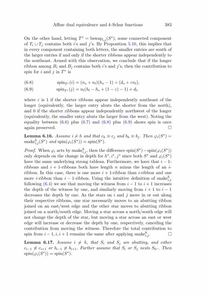
Affine dual equivalence and k-Schur functions 383
On the other hand, letting T ∗ = bswapi,j(S∗), some connected component
of Ti ∪ Tj contains both i’s and j’s. By Proposition 5.10, this implies thatin every component containing both letters, the smaller entries are south ofthe larger entries if and only if the shorter ribbons appear independently tothe southeast. Armed with this observation, we conclude that if the longerribbon among Bi and Bj contains both i’s and j’s, then the contribution tospin for i and j in T ∗ is
spinT ∗(i) = (ns + nl)(hs − 1) + (ds + εnl),(6.8)
spinT ∗(j) = nl(hl − hs + (1− ε)− 1) + dl,(6.9)
where ε is 1 if the shorter ribbons appear independently southeast of thelonger (equivalently, the larger entry abuts the shorter from the north),and 0 if the shorter ribbons appear independently northwest of the longer(equivalently, the smaller entry abuts the larger from the west). Noting theequality between (6.6) plus (6.7) and (6.8) plus (6.9) shows spin is onceagain preserved.
Lemma 6.16. Assume i = h and that ch ≡ cj and bh ≡ bj. Then ϕi(S∗) =
snakehi,j(S∗) and spin(ϕi(S
∗)) = spin(S∗).
Proof. When ϕi acts by snakehi,j , then the difference spin(S∗)− spin(ϕi(S∗))
only depends on the change in depth for h∗, i∗, j∗ since both S∗ and ϕi(S∗)
have the same underlying strong tableau. Furthermore, we have that i− 1-ribbons and i + 1-ribbons both have length n minus the length of an i-ribbon. In this case, there is one more i + 1-ribbon than i-ribbon and onemore i-ribbon than i − 1-ribbon. Using the intuitive definition of snakehi,jfollowing (6.4) we see that moving the witness from i− 1 to i+ 1 increasesthe depth of the witness by one, and similarly moving from i + 1 to i − 1decreases the depth by one. As the stars on i and j move in or out alongtheir respective ribbons, one star necessarily moves to an abutting ribbonjoined on an east/west edge and the other star moves to abutting ribbonjoined on a north/south edge. Moving a star across a north/south edge willnot change the depth of the star, but moving a star across an east or westedge will increase or decrease the depth by one, respectively, canceling thecontribution from moving the witness. Therefore the total contribution tospin from i− 1, i, i+ 1 remains the same after applying snakehi,j .
Lemma 6.17. Assume i = h, that Si and Sj are abutting, and eitherci−1 ≡ ci+1 or bi−1 ≡ bi+1. Further assume that Si or Sj nests Sh∗. Thenspin(ϕi(S
∗)) = spin(S∗).

384 Sami H. Assaf and Sara C. Billey
Figure 12: An example of ϕi acting via ϕi = doublehi,j .
Proof. This follows from Lemma 6.15 where bswapi,j is shown to preserve
spin.
Lemma 6.18. Assume i = h, that Si and Sj are abutting, and either ci−1 ≡ci+1 or bi−1 ≡ bi+1. Further assume that Bi or Bj nests Sh∗ but neither Si
nor Sj nests Sh∗. Then ϕi(S∗) = doublehi,j(S
∗) and spin(ϕi(S∗)) = spin(S∗).
Proof. We may assume, from the analysis in Lemma 6.10, that some h-
ribbon and j-ribbon share a head or tail. Also from Lemma 6.10, some h-
ribbon must appear independently of all i-ribbons. Furthermore, by Propo-
sition 5.10, if i- or j-ribbons appear independently of the other, then they
do so on the opposite side of abutting i- and j-ribbons from h-ribbons. Sup-
posing first that the combined lengths of an i-ribbon plus a j-ribbon is less
than n, reading from northwest to southeast or from southeast to northwest
one sees isolated h-ribbons followed by abutting i- and j-ribbons nesting
h-ribbons. There are then three options for what follows: isolated j-ribbons;
isolated abutting i- and h-ribbons; or no further i-, j- or h-ribbons. For ex-
ample, see Figure 12. Note that, in particular, S∗ has isolated j-ribbons if
and only if doublehi,j(S∗) has isolated abutting i- and h-ribbons.
To assess the contributions to spin, assume that S∗ has no isolated abut-
ting i- and h-ribbons, as in the right hand side of Figure 12. Let hw and
dw denote the height and depth of the starred h-ribbon, respectively, and
let nw denote the number of isolated witness ribbons. For the example, we
have nw = 1, hw = 1, dw = 0. Let nl be the number of i-ribbons, each with
height hl and the starred one with depth dl. Let ns be the number of isolated
j-ribbons, and let hs and ds denote the height and depth, respectively, of
j-ribbons. For the example, we have nl = 2, hl = 2, dl = 1 and ns = 1,
hs = 2, ds = 0.
The contribution to spin from i−1, i, i+1 in S∗, where S∗ has no isolated
abutting i- and h-ribbons, is given by

Affine dual equivalence and k-Schur functions 385
spinS∗(h) = (nl + nw)(hw − 1) + dw,(6.10)
spinS∗(i) = nl(hl − 1) + dl,(6.11)
spinS∗(j) = (nl + ns)(hs − 1) + ds.(6.12)
Following the description of how doublehi,j acts on these ribbons, we maysimilarly compute the contributions of i − 1, i, i + 1 to the spin of T ∗ =doublehi,j(S
∗). With h and j defined relative to T ∗, we have
spinT ∗(h) = (nl + nw + ns)(hw − 1) + (dw + εns),(6.13)
spinT ∗(i) = (nl + ns)(hs − hw + (1− ε)− 1) + ds,(6.14)
spinT ∗(j) = nl(hl + hw − (1− ε)− 1) + dl,(6.15)
where, similar to before, ε is 0 if the witness originally existed only to theleft of abutting i- and j-ribbons and 1 otherwise. Adding the contributionsin either case miraculously yields the same result, thereby showing that thespin statistic is preserved.
If i-ribbons and j-ribbons have lengths adding to n, we regard the abut-ting i- and j-ribbons which together nest an h-ribbon as abutting pairs, andthe leftover max(i, j)-ribbon as isolated. For example, in Figure 10, we re-gard the left side as having 1-ribbons abutting 2-ribbons from the west withan isolated abutting 2-ribbon and 3-ribbon to the northwest, and the rightside we regard as having 2-ribbons abutting 3-ribbons from the west with anisolated 3-ribbon to the northwest. That is to say, Figure 10 is the same asFigure 12 for the purposes of calculating spin. In this case, note that S∗ hasno isolated abutting i- and h-ribbons precisely when h = i− 1. Moreover, inthis case we always have ns = 1. With this alteration, the analysis of spinis precisely as before, again showing that spin is preserved.
The results in Theorem 6.12 and Proposition 6.14 naturally extend toskew partitions as well since the proofs only involve intervals of rank 3 inthe n-core poset.
Theorem 6.19. Let μ ⊂ ν be n-cores of lengths �(μ) = p and �(ν) = q.Then, for p < i < q, the map ϕi is a well-defined, spin preserving, involutionon all starred strong skew tableaux for ν/μ. In particular, spin is constanton affine dual equivalence classes.
7. A graph on starred strong tableaux
In this section, we construct a vertex-signed, edge-colored graph from ourelementary affine dual equivalence map ϕi. The main goal of this section

386 Sami H. Assaf and Sara C. Billey
is to show that this graph is, in fact, an LSP2 graph by Definition 4.5.In order to establish this, we introduce two operations on starred strongtableaux which together show that there are only finitely many isomorphismtypes for 2-colored connected components. The reduction to finitely manyisomorphism types can be viewed as an (incomplete) analog of the jeu detaquin algorithm for starred strong tableaux. This analogy is summarizedin Remark 7.12.
Definition 7.1. For an n-core ν, the affine dual equivalence graph G(n)ν is
the signed, colored graph with vertex set Vν given by the set of all starredstrong tableaux S∗ of shape ν, with signature function σ(S∗) obtained fromthe reading word on the starred letters in S∗, and for each 1 < i < �(ν),the set of i-colored edges, Ei, is the set of all pairs {S∗, ϕi(S
∗)} such thatS∗ = ϕi(S
∗). This definition also extends to skew shapes ν/μ in the n-coreposet. For S∗ ∈ SST∗(ν/μ, n), let [S∗] denote the connected component of
the affine dual equivalence graph G(n)ν/μ containing S∗.
For example, for n = 3 and μ = (5, 3, 1) the affine dual equivalence graphis shown on page 395.
Recall that ϕi is an involution which preserves the spin statistic by The-orem 6.19. In order to justify our terminology of affine dual equivalence. Wewant to prove that the graph induced by these involutions satisfies Axioms1, 2, 3, 5 from Definition 4.2 and local Schur positivity on all two adjacentcolored connected components. Thus each affine dual equivalence graph isLSP2. The key will be reducing local Schur positivity to a finite verification.The reduction is achieved with the help of flattening rows and squashingand/or cloning columns.
7.1. The flattening map
Here we define an iterative procedure to flatten an n-core partition downto an m-core partition for any 1 ≤ m < n. We will extend this procedureto starred strong tableaux in a way that commutes with the affine dualequivalence involutions.
Definition 7.2. For any m+1-core λ and any 1 ≤ d ≤ m+1, define λ(d) tobe the unique partition associated to the binary string obtained by removingall beads and spacers with content congruent to d modulo m + 1 from theabacus of λ. In particular, λ(d) is an m-core.
We note that the above definition makes sense in light of Remark 5.1 andthe characterization of n-cores in terms of the n-rod abacus. For example,regarding (7, 4, 4, 2, 2) as a 4-core, (7, 4, 4, 2, 2)(2) is the 3-core (6, 4, 2).

Affine dual equivalence and k-Schur functions 387
Remark 7.3. For n-cores μ ⊂ ν, if some transposition sequence from μ to νleaves rod d fixed then every transposition sequence from μ to ν leaves rod dfixed. This follows from the observation that any saturated chain from μ toν can be obtained from any other by some sequence of interval exchanges,none of which may change which rods are fixed.
Proposition 7.4. Let μ ⊂ ν be m + 1-cores such that some (equivalently,every) transposition sequence from μ to ν fixes rod d. Then the interval [μ, ν]in the m+1-core poset is isomorphic to [μ(d), ν(d)] in the m-core poset. Thisisomorphism extends to a bijection on skew strong tableaux which preservesthe number of i-ribbons for each i.
Remark 7.5. Proposition 7.4 can be used in reverse: given μ < ν in them-core poset, we can lift the interval [μ, ν] to an isomorphic interval in them+ 1-core posets with the same nice implications on strong tableaux. Thismap is implemented by using the inverse procedure of adding in an extrarod between any two existing rods. This can be done precisely when thelength of the inserted rod never has length weakly between the length oftwo interchanging rods. For instance, we may always take the rod to belonger than all other rods or shorter than all other rods.
Proof. Since the length of rod d for each m+ 1-core λ in the interval [μ, ν]is constant, the covering relations in the m+1-core poset restricted to [μ, ν]depend on rod d only in the sense that it must not have length weaklybetween that of the two exchanging rods, covering relations in mapping[μ, ν] down to the m-core poset are preserved. Since rod d is fixed in everytransposition sequence from μ to ν, the map from λ to λ(d) is surjective onthe interval [μ(d), ν(d)].
Conversely, given any m-core γ ∈ [μ(d), ν(d)], we can lift it to an m+ 1-core by reversing the procedure. The reverse procedure is injective and alsopreserves the covering relations. Hence the intervals are isomorphic.
The bijection on skew strong tableaux is obtained in the obvious way,by mapping the saturated chain
S = (μ = μ0 ⊂ μ1 ⊂ μ2 ⊂ · · · ⊂ μk = ν)

388 Sami H. Assaf and Sara C. Billey
to the chain
S(d) = (μ(d) = μ(d)0 ⊂ μ
(d)1 ⊂ μ
(d)2 ⊂ · · · ⊂ μ
(d)k = ν(d)).
To see that this bijection preserves the number of i-ribbons, recall fromCorollary 5.4 that the number of i-ribbons of a strong tableau is equal tothe difference in length of the interchanging rods taking λi−1 to λi. Sincethe map from m + 1-cores to m-cores preserves the relative lengths of allrods other than rod d, this number is clearly preserved.
By Proposition 7.4, the following map is well defined.
Definition 7.6. Let μ ⊂ ν be m + 1-cores such that some (equivalently,every) transposition sequence from μ to ν does not touch rod d. Define theflattening map
fld : SST∗(ν/μ,m+ 1) −→ SST∗(ν(d)/μ(d),m)
sending S∗ ∈ SST∗(ν/μ,m + 1) to the underlying strong tableau S(d) withthe stars placed on each i-ribbon in such a way as to preserve the depth.
Note that the flattening map does not, in general, preserve the spinstatistic because it can shorten the height of ribbons.
Proposition 7.7. Let μ ⊂ ν be m + 1-cores such that some transposi-tion sequence from μ to ν does not touch rod d. The flattening map fld :SST∗(ν/μ,m + 1) −→ SST∗(ν(d)/μ(d),m) is a bijection preserving the sig-nature of a starred strong tableau and it commutes with the involutions ϕi
for all 1 < i < �(ν)− �(μ).
Proof. To see fld preserves the signature σ(S∗), recall from Definition 5.5and Corollary 5.6 that the content of i∗ is determined by an excess bead onthe longer rod in the ith exchange on the n-rod abacus. Since the relativeorder among the beads on the abacus is unchanged by the procedure inDefinition 7.2, the contents of i∗, (i+ 1)∗ will form a decent in σ(S∗) if andonly if there is a corresponding descent in σ(fld(S
∗)). This proves σ(S∗) =σ(fld(S
∗)).To show fld(ϕi(S
∗)) = ϕi(fld(S∗)), simply note that the cases in the defi-
nition of ϕi depend only on the types of rod exchanges in the corresponding3-interval of the m+ 1 or m-core poset respectively. But, the relative orderamong the endpoints of the exchanging rods and the isomorphism type ofthe interval are persevered by the flattening map. Hence the flattening mapand the involution commute.

Affine dual equivalence and k-Schur functions 389
Corollary 7.8. Let μ ⊂ ν be n-cores with ν lying r ranks above μ. If2r < n, then for m = 2r, there exists m-cores μ ⊂ ν such that there existsa bijection from SST∗(ν/μ, n) to SST∗(ν/μ,m) that preserves the signatureand commutes with the involutions ϕi for all 1 < i < �(ν) − �(μ). Thus,the affine dual equivalence graphs of ν/μ and ν/μ are isomorphic as signedcolored graphs.
Proof. If rank(ν) − rank(μ) = r, then every transposition sequence from μto ν has exactly r elements and at most 2r distinct subscripts. Therefore, byProposition 7.4, we can find an interval isomorphic to [μ, ν] in the m-coreposet after removing all fixed rods on this interval. This isomorphism pre-serves the number of i-ribbons for each i. Thus, it extends to an isomorphismfrom SST∗(ν/μ, n) to SST∗(ν/μ,m) by requiring the depth of the starred i-ribbon to be constant under this map for each i. The length of the i-ribbonsand the contents of the i-ribbons can change under this bijection. However,the relative order among the contents of the ribbons will not change sincethe depth is preserved and the length differences of the remaining rods areexactly the same. We concluded that the signature is preserved under thebijection. Furthermore, the conditions for the witness and for the involutionsϕi for all 1 < i < �(ν)−�(μ) only depend on the relative order of the contentsand lengths of consecutive ribbons. These relative orders will be unchangedby the bijection on starred strong tableaux. This allows us to conclude thatthe affine dual equivalence graphs of ν/μ and ν/μ are isomorphic as signedcolored graphs.
7.2. The cloning map
Whereas flattening removes rows of the abacus, cloning adds columns. Anal-ogous to flattening, we will define cloning on starred strong tableaux so thatit preserves the signatures. In some cases, cloning commutes with the affinedual equivalence operators ϕi.
Definition 7.9. For any n-core μ, define μ(j) to be the unique partitionassociated to the abacus obtained by cloning the column of the n-rod aba-cus of μ containing positions j, j + 1, . . . , j + n − 1. Specifically, let β bethe binary string encoding the abacus for μ. Then μ(j) is the abacus asso-ciated to the string obtained from β by inserting a copy of the substringβj , βj+1, . . . , βj+n−1 into the abacus for μ between positions j − 1 and j.
Cloning a column has the effect of extending some of the rods in then-rod abacus, hence μ(j) is also an n-core. To see the effect of cloning onpartitions, consider taking (5, 2, 2) regarded as a 4-core and cloning the

390 Sami H. Assaf and Sara C. Billey
column beginning with content 0. This gives (5, 2, 2)(0) = (7, 4, 4, 2, 2), asdepicted below.
Observe that for fixed μ, different values for j can lead to the same n-core μ(j). For instance, taking any j ∈ {−4, . . . , 0} results in (5, 2, 2)(j) =(7, 4, 4, 2, 2).
In order for flattening to preserve a covering relation in the n-core poset,the transposition sequence simply needs to avoid the rod being removed.The situation for cloning is more subtle. Covering relations are not alwayspreserved even when the replicated column is disjoint from the indexingtransposition. It is immediate from Proposition 5.3 that if tr,sμ > μ is acovering relation in the n-core poset, then (tr,sμ)(j) covers μ(j) in the n-coreposet if and and only if for every r < h ≤ s the relative order of the lengthsof rods h, r and s is the same in both μ and μ(j). We call such a j a cloneableindex for μ ⊂ tr,sμ. More generally, j is a cloneable index for the interval[μ, ν] provided cloning the column beginning at j of every core partitionin the interval results in another isomorphic interval in the n-core poset.This happens if and only if no rod in the n-rod abacus representing anyelement in the interval has a rightmost bead of content j, j+1, . . . , j+n−1.Similarly, we say j is a cloneable index for S∗ ∈ SST∗(ν/μ, n) provided j isa cloneable index for [μ, ν]. The clone of S∗, denoted clj(S
∗), is defined to bethe saturated chain obtained from S by cloning, the column beginning withj in each n-rod abacus in the chain and leaving all the stars with contentless than j at the same depth and increasing the depth by 1 for all stars withcontent at least j. Note, all i-ribbons will have the same shape in S∗ andclj(S
∗) since the relative order of the rod lengths is unchanged by cloning acolumn. See Figure 13 for example.
Observe that if S∗ ∈ SST∗(ν/μ, n) and j is a cloneable index for S∗, thenj is a cloneable index for every other starred strong tableau in SST∗(ν/μ, n)as well since the definition of a cloneable index only depends on the interval[μ, ν].
Definition 7.10. Assume that S∗ has a cloneable index at j and thatT ∗ = clj(S
∗) ∈ SST∗(β/α, n). Define the cloning map on components
clj : [S∗] −→ SST∗(β/α, n)

Affine dual equivalence and k-Schur functions 391
Figure 13: An example of the cloning map on a starred strong tableau. Thecloned cells are red in the electronic version.
by cloning each starred strong tableaux in [S∗] at the column beginning withj. The inverse map to cloning, when it is defined, will be denoted by
sqj : [T∗] −→ [S∗]
and we call it the squashing map.
As with the flattening map, the cloning map does not, in general, pre-serve the spin statistic since it may alter the number of i-ribbons and/or itmay alter the depth of the starred ribbons. Nonetheless, once the cloningmap commutes with the ϕi’s on a connected component of an affine dualequivalence graph then we can clone the same column any number of timesand get an isomorphic component.
The following proposition is the analog of Proposition 7.7.
Proposition 7.11. Assume that S∗ ∈ SST∗(ν/μ, n) has a cloneable index atj and that T ∗ = clj(S
∗). Further assume that cloning the column beginningat j commutes with the involutions ϕi for all 1 < i < �(ν) − �(μ) on thecomponent [S∗]. Then j is a cloneable index for every starred strong tableauxin [T ∗]. Moreover, if U∗ = clj(T
∗), then clj : [T ∗] −→ [U∗] is a bijectionpreserving the signature of each starred strong tableau and it commutes withthe involutions ϕi for all 1 < i < �(ν) − �(μ). Thus, [S∗] ≈ [T ∗] ≈ [U∗] assigned, colored graphs.
Proof. The fact that j is again a cloneable index for T ∗ follows directly fromthe characterization of j being a cloneable index for the interval containingS∗ in terms of rod lengths.
To see that [T ∗] is isomorphic to [U∗] as signed colored graphs, onemust check that the affine dual equivalence maps ϕi commute with thecloning map from [T ∗] to [U∗]. This follows since the conditions for the

392 Sami H. Assaf and Sara C. Billey
affine dual equivalence map on rank 3 intervals are unchanged at each stepby removing n consecutive content diagonals that contains no head or tail ofa starred ribbon in any of the starred strong tableaux in [U∗] and that thecells in those n diagonals must necessarily be a copy of the next n-translatedown.
Remark 7.12. As a consequence of Propositions 7.7 and 7.11, we observethat the process of flattening and squashing a component in an affine dualequivalence graph as much as possible is similar to applying the necessaryjeu de taquin slides which bring together all of the connected componentsin a skew tableaux by removing empty rows and columns. Note, both flat-tening and cloning/squashing can change the spin statistic even when theycommute with affine dual equivalence on a component. Thus a completeanalog of jeu de taquin generalizing these moves would need to keep trackof powers of t separately from the algorithm.
7.3. Local Schur positivity
Our next goal is to show that there are only a small number of isomorphismclasses of connected components of rank 4 affine dual equivalence graphs.Recall that a starred strong tableau S∗ on an interval [μ, ν] has ribbonslabeled 1, 2, . . . , �(ν)− �(μ). We say S∗ has rank r provided r = �(ν)− �(μ).The component [S∗] of the affine dual equivalence graph on ν/μ has edgeslabeled 2, 3, . . . , r − 1 and each vertex has a signature of length r − 1.
Lemma 7.13. Let S∗ ∈ SST∗(ν/μ, n) be a starred strong tableau of rankk = 4. Then [S∗] has a Schur positive generating function. In fact, eachsuch [S∗] is either an isolated vertex, or a path with either 2 or 4 edges withalternating color labels. See Figure 14.
This lemma can be proved in two ways. One approach is to do a computerverification by identifying a set of dual equivalence classes which containall possible isomorphism types after flattening and squashing as much aspossible. The lisp code used for this approach can be found in
http://www.math.washington.edu/~billey/kschur/verifier.faster.lisp.
The second approach is based on the reading words of the starred strongtableaux, see [3].
Remark 7.14. An extensive computer exploration for all possible isomor-phism types for affine dual equivalence graphs of rank 5 was undertaken.As of November of 2011, we have observed 326 distinct isomorphism types

Affine dual equivalence and k-Schur functions 393
Figure 14: All 7 possible isomorphism types of connected components ofaffine dual equivalence graphs of rank 4.
which can be viewed in
http://www.math.washington.edu/~billey/kschur/d-graphs-11-2011.pdf.
Note for comparison, there are only 25 isomorphism types for rank 5 graphsfor LLT polynomials as defined in Section 8.
Theorem 7.15. For any pair of n-core partitions μ ⊂ ν, the affine dual
equivalence graph G(n)ν/μ is a D graph which is locally Schur positive for 2-
colored edges and for which spin is constant on connected components.
Proof. By Proposition 6.14, the involutions ϕi preserve the spin statistic,
hence spin is constant on connected components of G(n)ν/μ.
To prove G(n)ν/μ is a D graph, we must verify the axioms in Definition 4.5.
Axiom 1 follows from Theorem 6.12 where ϕi is shown to be an involutionwhich switches the sign appropriately. Axioms 2 and 5 follow from the factthat ϕi affects only i−1, i and i+1-ribbons. Axiom 3 and the LSP2 property
both follow from Lemma 7.13 since every connected component of G(n)ν/μ
restricted to Ei−1 ∪Ei is isomorphic to a component of a rank 4 affine dualequivalence graph replacing the edge labels 2, 3 by i− 1, i respectively.

394 Sami H. Assaf and Sara C. Billey
Note that affine dual equivalence graphs need not satisfy Axiom 4 ofDefinition 4.2. It is not known if affine dual equivalence graphs satisfy Ax-iom 6.
8. Connections with LLT, Macdonald polynomials andBeyond
The primary interest in k-Schur functions originally was the conjecture ofLapointe, Lascoux and Morse that these functions straddle the gap betweenMacdonald polynomials and Schur functions. That is, when μ is a k-boundedpartition, they conjecture
(8.1) Hμ(X; q, t) =∑ν≤μ
K(k)ν,μ(q, t) s
(k)ν (X; t),
where K(k)ν,μ(q, t) ∈ N[q, t], and
(8.2) s(k)ν (X; t) =∑λ≤ν
C(k)λ,ν(t) sλ(X),
where C(k)λ,ν(t) ∈ N[t].
The Macdonald polynomials, the LLT polynomials, and the k-Schurfunctions using the definition given in this paper, expand positively in thebasis of fundamental quasisymmetric functions with indexing sets based ongeneralized tableaux. See [10] for details on the Macdonald and LLT ex-pansions. We now have a signed colored graph structure on the generalizedtableaux in each case by the construction in [2] and Theorem 7.15. It is anopen problem to describe how these graphs relate to each other. Towardfinding such a connection, we have identified a D graph isomorphism θ be-tween the graph of starred strong tableaux on the 2-core (m,m − 1, . . . , 1)and the graph of standard filling of the m-tuple ((1), . . . , (1)) each embeddedat content 0. Furthermore,
(m2
)− spin(S∗) = inv(θ(S∗)).
In fact, for any family of functions expressible in terms of fundamentalquasisymmetric functions which are conjectured to be Schur positive, onecan look for a signed-colored graph structure or analog of dual equivalenceon the indexing set which refines the Schur positivity question to connectedcomponents. Another example of this phenomena arises in the work of Loehrand Warrington [25]. They showed that the plethysm of two Schur functionshas a nice expansion in terms of fundamental quasisymmetric functions in-dexed by a family of objects in analogy with standard tableaux. Is there a

Affine dual equivalence and k-Schur functions 395
Figure 15: The poset of 3-cores lying below (5, 3, 1), with edge weights givingthe spin contributions of possible starrings.
nice signed-colored graph structure for these objects? Also, the Stanley sym-metric functions are indexed by reduced expressions for permutations andexpand positively in terms of both fundamental quasisymmetric functionsand Schur functions. Is there a family of standard objects and an analog ofa dual equivalence graph that goes with the Stanley symmetric functions?
Appendix A. Examples
In this appendix we give the quasisymmetric and Schur expansion for the
k-Schur function s(2)(2,2,1). We compute this using the interval [∅, (5, 3, 1)] of
the 3-core poset (Figure 15) and the corresponding D graph on all starredstrong tableaux of shape (5, 3, 1) regarded as a 3-core (Figure 16).
Thus, we obtain from Figure 16 that
s(2)(2,2,1) = Q−+−− + Q−−+− + t Q++−− + (1 + t) Q+−−+
+ (2t+ t2) Q−++− + (1 + 2t+ t2) Q+−+−
+ (1 + 2t+ t2) Q−+−+ + t Q−−++ + (t2 + t3) Q+++−
+ (t+ 2t2 + t3) Q++−+ + (t+ 2t2 + t3) Q+−++
+ (t2 + t3) Q−+++ + t4Q++++
= s(2,2,1) + ts(3,1,1) + (t+ t2)s(3,2) + (t2 + t3)s(4,1) + t4s(5).
Acknowledgments
We would like to thank Nantel Bergeron, Andrew Crites, Adriano Garsia,Jim Haglund, Mark Haiman, Steve Mitchell, Jennifer Morse, Austin Robertsand Mike Zabrocki for inspiring conversations on this topic, and an anony-mous referee for many useful comments.

396 Sami H. Assaf and Sara C. Billey
Figure 16: The D graph on starred strong tableaux of shape (5, 3, 1) regardedas a 3-core.
References
[1] S. Assaf (2007). The Schur expansion of Macdonald polynomials.
Preprint. MR2710706
[2] S. Assaf. Dual equivalence graphs I: A combinatorial proof of LLT and
Macdonald positivity. arXiv:1005.3759, originally 2008, revised 2011.
MR2721449
[3] S. H. Assaf. On dual equivalence and Schur positivity. ArXiv e-prints,
June 2011.
[4] C. Berg, B. Jones, and M. Vazirani (2009). A bijection on core partitions

Affine dual equivalence and k-Schur functions 397
and a parabolic quotient of the affine symmetric group. J. Combin.Theory Ser. A 116(8) 1344–1360. MR2568803
[5] A. Bjorner and F. Brenti (1996). Affine permutations of type A. Elec-tron. J. Combin. 3(2), Research Paper 18, approx. 35 pp. (electronic).The Foata Festschrift. MR1392503
[6] W. Fulton (1997). Young Tableaux; With Applications To Representa-tion Theory And Geometry, volume 35 of London Mathematical SocietyStudent Texts. Cambridge University Press, New York. MR1464693
[7] A. M. Garsia and M. Haiman (1993). A graded representation modelfor Macdonald’s polynomials. Proc. Natl. Acad. Sci. USA 90(8) 3607–3610. MR1214091
[8] I. M. Gessel (1984). Multipartite P -partitions and inner products ofskew Schur functions. In: Combinatorics and Algebra (Boulder, Colo.,1983), Vol. 34, Contemp. Math., Amer. Math. Soc., Providence, RI, pp.289–317. MR0777705
[9] J. Haglund (2004). A combinatorial model for the Macdonald polyno-mials. Proc. Natl. Acad. Sci. USA 101(46) 16127–16131 (electronic).MR2114585
[10] J. Haglund, M. Haiman, and N. Loehr (2005). A combinatorial for-mula for Macdonald polynomials. J. Amer. Math. Soc. 18(3) 735–761(electronic). MR2138143
[11] M. Haiman (2001). Hilbert schemes, polygraphs and the Macdonaldpositivity conjecture. J. Amer. Math. Soc. 14(4) 941–1006 (electronic).MR1839919
[12] M. D. Haiman (1992). Dual equivalence with applications, including aconjecture of Proctor. Discrete Math. 99(1-3) 79–113. MR1158783
[13] C. R. H. Hanusa and B. C. Jones. Abacus models for parabolic quotientsof affine Weyl groups. arXiv:1105.5333, May 2011. MR2921615
[14] G. James and A. Kerber. The representation theory of the symmet-ric group, Vol. 16, Encyclopedia of Mathematics and its Applications.Addison-Wesley Publishing Co., Reading, Mass., 1981. With a fore-word by P. M. Cohn; With an introduction by Gilbert de B. Robinson.MR0644144
[15] T. Lam (2008). Schubert polynomials for the affine Grassmannian. J.Amer. Math. Soc. 21(1) 259–281 (electronic). MR2350056
398 Sami H. Assaf and Sara C. Billey
[16] T. Lam, L. Lapointe, J. Morse, and M. Shimozono. k-shape poset
and branching of k-Schur functions. Preprint, 2010. arXiv:1007.5334v1.
MR2741963
[17] T. Lam, L. Lapointe, J. Morse, and M. Shimozono (2010). Affine inser-
tion and Pieri rules for the affine Grassmannian. Mem. Amer. Math.
Soc. 208(977). MR2741963
[18] L. Lapointe, A. Lascoux, and J. Morse (2003). Tableau atoms and a
new Macdonald positivity conjecture. Duke Math. J. 116(1) 103–146.
MR1950481
[19] L. Lapointe and J. Morse (2003). Schur function analogs for a filtration
of the symmetric function space. J. Combin. Theory Ser. A 101(2)
191–224. MR1961543
[20] L. Lapointe and J. Morse (2003). Schur function identities, their
t-analogs, and k-Schur irreducibility. Adv. Math. 180(1)222–247.
MR2019223
[21] L. Lapointe and J. Morse (2005). Tableaux on k + 1-cores, reduced
words for affine permutations, and k-Schur expansions. J. Combin.
Theory Ser. A 112(1)44–81. MR2167475
[22] L. Lapointe and J. Morse (2007). A k-tableau characterization of k-
Schur functions. Adv. Math. 213(1) 183–204. MR2331242
[23] A. Lascoux (2001). Ordering the affine symmetric group. In Alge-
braic Combinatorics and Applications (Goßweinstein, 1999), Springer,
Berlin, pp. 219–231. MR1851953
[24] A. Lascoux, B. Leclerc, and J.-Y. Thibon (1997). Ribbon tableaux,
Hall-Littlewood functions, quantum affine algebras, and unipotent va-
rieties. J. Math. Phys. 38(2) 1041–1068. MR1434225
[25] N. A. Loehr and G. S. Warrington (2012). Quasisymmetric expansions
of Schur-function plethysms. Proc. Amer. Math. Soc. 140(4) 1159–
1171. MR2869102
[26] I. G. Macdonald (1988). A new class of symmetric functions. Actes du
20e Seminaire Lotharingien 372 131–171.
[27] I. G. Macdonald (1995). Symmetric Functions and Hall Polynomials,
2nd ed. Oxford Mathematical Monographs. The Clarendon Press Ox-
ford University Press, New York. With contributions by A. Zelevinsky,
Oxford Science Publications. MR1354144

Affine dual equivalence and k-Schur functions 399
[28] K. Misra and T. Miwa (1990). Crystal base for the basic representationof Uq(sl(n)). Comm. Math. Phys. 134(1) 79–88. MR1079801
[29] R. P. Stanley (1997). Enumerative Combinatorics. Vol. 1, Vol. 49 Cam-bridge Studies in Advanced Mathematics. Cambridge University Press,Cambridge. With a foreword by Gian-Carlo Rota; Corrected reprint ofthe 1986 original. MR1090542
Sami H. Assaf
Department of Mathematics
University of Southern California
3620 S Vermont Ave KAP 104
Los Angeles, CA 90089-2532
USA
E-mail address: [email protected]
Sara C. Billey
Mathematics Department
University of Washington
Box 354350
Seattle, WA 98105
USA
E-mail address: [email protected]
Received January 6, 2012


![arXiv:1801.04257v3 [math.DG] 1 Mar 2019 · 2019. 3. 4. · arXiv:1801.04257v3 [math.DG] 1 Mar 2019 ON PROJECTIVE AND AFFINE EQUIVALENCE OF SUB-RIEMANNIAN METRICS FRED´ ´ERIC JEAN,](https://static.fdocuments.net/doc/165x107/60cebdf9d6e288136150cf7c/arxiv180104257v3-mathdg-1-mar-2019-2019-3-4-arxiv180104257v3-mathdg.jpg)