2014-2015

Preethi Nair

CARLETON UNIVERSITY

Department of Mechanical and

Aerospace Engineering

2014-2015

MAAE 4907 Formula Student

AERODYNAMICS

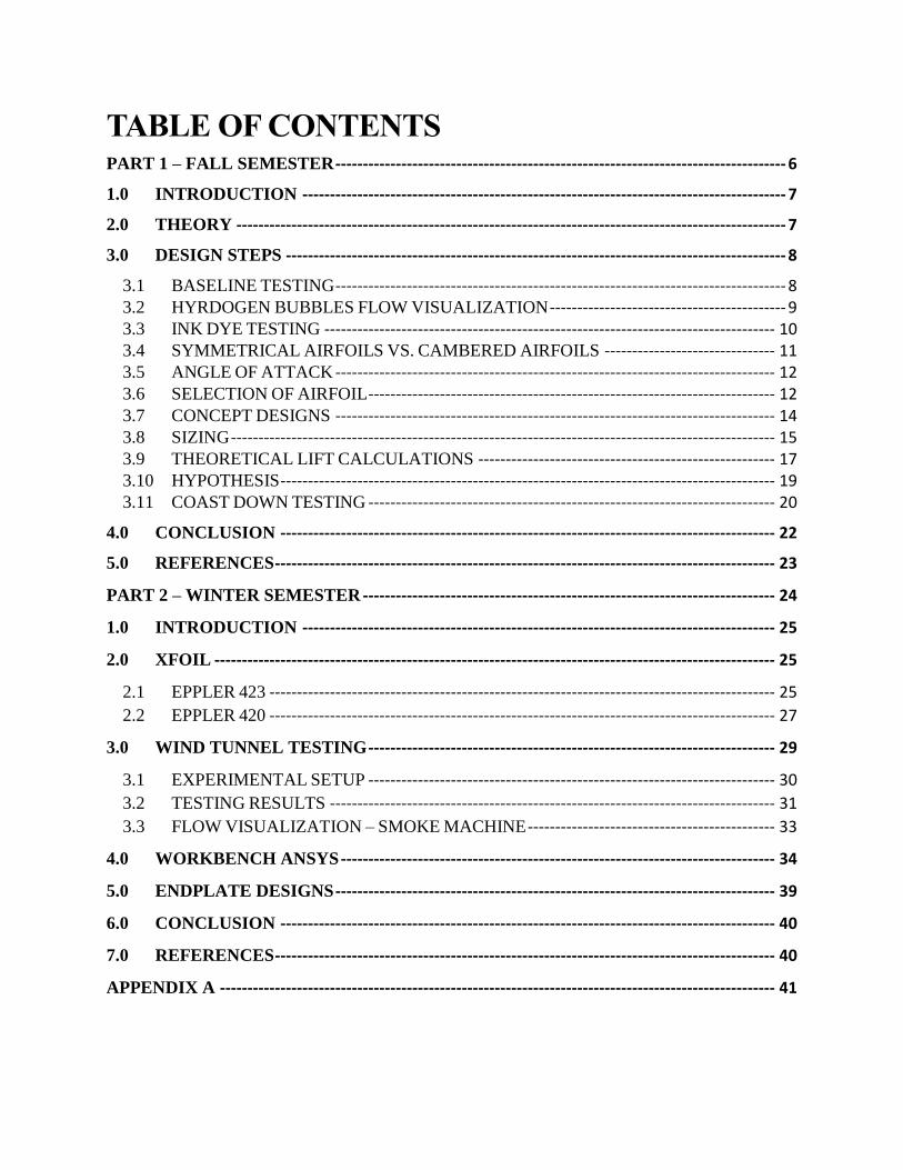
TABLE OF CONTENTS PART 1 – FALL SEMESTER ---------------------------------------------------------------------------------- 6

1.0 INTRODUCTION ---------------------------------------------------------------------------------------- 7

2.0 THEORY ---------------------------------------------------------------------------------------------------- 7

3.0 DESIGN STEPS ------------------------------------------------------------------------------------------- 8

3.1 BASELINE TESTING ---------------------------------------------------------------------------------- 8 3.2 HYRDOGEN BUBBLES FLOW VISUALIZATION ------------------------------------------- 9 3.3 INK DYE TESTING ---------------------------------------------------------------------------------- 10 3.4 SYMMETRICAL AIRFOILS VS. CAMBERED AIRFOILS ------------------------------- 11 3.5 ANGLE OF ATTACK -------------------------------------------------------------------------------- 12 3.6 SELECTION OF AIRFOIL -------------------------------------------------------------------------- 12 3.7 CONCEPT DESIGNS -------------------------------------------------------------------------------- 14 3.8 SIZING --------------------------------------------------------------------------------------------------- 15 3.9 THEORETICAL LIFT CALCULATIONS ------------------------------------------------------ 17 3.10 HYPOTHESIS ------------------------------------------------------------------------------------------ 19 3.11 COAST DOWN TESTING -------------------------------------------------------------------------- 20

4.0 CONCLUSION ------------------------------------------------------------------------------------------ 22

5.0 REFERENCES ------------------------------------------------------------------------------------------- 23

PART 2 – WINTER SEMESTER --------------------------------------------------------------------------- 24

1.0 INTRODUCTION -------------------------------------------------------------------------------------- 25

2.0 XFOIL ------------------------------------------------------------------------------------------------------ 25

2.1 EPPLER 423 -------------------------------------------------------------------------------------------- 25

2.2 EPPLER 420 -------------------------------------------------------------------------------------------- 27

3.0 WIND TUNNEL TESTING -------------------------------------------------------------------------- 29

3.1 EXPERIMENTAL SETUP -------------------------------------------------------------------------- 30

3.2 TESTING RESULTS --------------------------------------------------------------------------------- 31

3.3 FLOW VISUALIZATION – SMOKE MACHINE --------------------------------------------- 33

4.0 WORKBENCH ANSYS ------------------------------------------------------------------------------- 34

5.0 ENDPLATE DESIGNS -------------------------------------------------------------------------------- 39

6.0 CONCLUSION ------------------------------------------------------------------------------------------ 40

7.0 REFERENCES ------------------------------------------------------------------------------------------- 40

APPENDIX A ----------------------------------------------------------------------------------------------------- 41

LIST OF FIGURES

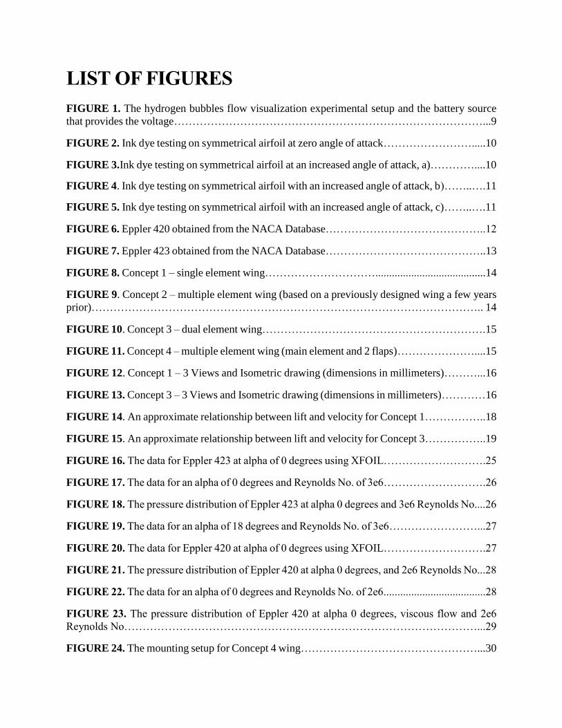
FIGURE 1. The hydrogen bubbles flow visualization experimental setup and the battery source

that provides the voltage…………………………………………………………………………...9

FIGURE 2. Ink dye testing on symmetrical airfoil at zero angle of attack…………………….....10

FIGURE 3.Ink dye testing on symmetrical airfoil at an increased angle of attack, a)…………....10

FIGURE 4. Ink dye testing on symmetrical airfoil with an increased angle of attack, b)……..….11

FIGURE 5. Ink dye testing on symmetrical airfoil with an increased angle of attack, c)……..….11

FIGURE 6. Eppler 420 obtained from the NACA Database……………………………………..12

FIGURE 7. Eppler 423 obtained from the NACA Database……………………………………..13

FIGURE 8. Concept 1 – single element wing…………………………........................................14

FIGURE 9. Concept 2 – multiple element wing (based on a previously designed wing a few years

prior)…………………………………………………………………………………………….. 14

FIGURE 10. Concept 3 – dual element wing…………………………………………………….15

FIGURE 11. Concept 4 – multiple element wing (main element and 2 flaps)…………………....15

FIGURE 12. Concept 1 – 3 Views and Isometric drawing (dimensions in millimeters)………...16

FIGURE 13. Concept 3 – 3 Views and Isometric drawing (dimensions in millimeters)…………16

FIGURE 14. An approximate relationship between lift and velocity for Concept 1……………..18

FIGURE 15. An approximate relationship between lift and velocity for Concept 3……………..19

FIGURE 16. The data for Eppler 423 at alpha of 0 degrees using XFOIL……………………….25

FIGURE 17. The data for an alpha of 0 degrees and Reynolds No. of 3e6……………………….26

FIGURE 18. The pressure distribution of Eppler 423 at alpha 0 degrees and 3e6 Reynolds No....26

FIGURE 19. The data for an alpha of 18 degrees and Reynolds No. of 3e6……………………...27

FIGURE 20. The data for Eppler 420 at alpha of 0 degrees using XFOIL……………………….27

FIGURE 21. The pressure distribution of Eppler 420 at alpha 0 degrees, and 2e6 Reynolds No...28

FIGURE 22. The data for an alpha of 0 degrees and Reynolds No. of 2e6.....................................28

FIGURE 23. The pressure distribution of Eppler 420 at alpha 0 degrees, viscous flow and 2e6

Reynolds No……………………………………………………………………………………...29

FIGURE 24. The mounting setup for Concept 4 wing…………………………………………...30

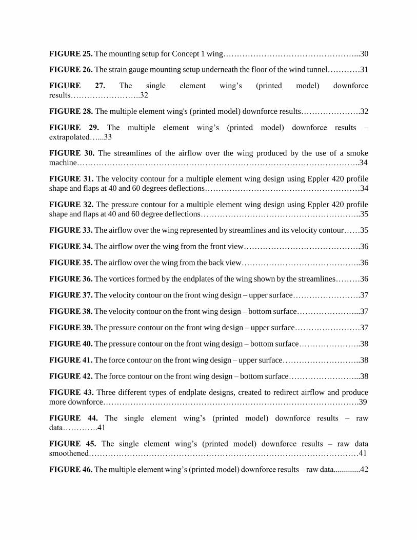
FIGURE 25. The mounting setup for Concept 1 wing…………………………………………...30

FIGURE 26. The strain gauge mounting setup underneath the floor of the wind tunnel…………31

FIGURE 27. The single element wing’s (printed model) downforce

results……………………..32

FIGURE 28. The multiple element wing's (printed model) downforce results………………….32

FIGURE 29. The multiple element wing’s (printed model) downforce results –

extrapolated…...33

FIGURE 30. The streamlines of the airflow over the wing produced by the use of a smoke

machine…………………………………………………………………………………………..34

FIGURE 31. The velocity contour for a multiple element wing design using Eppler 420 profile

shape and flaps at 40 and 60 degrees deflections…………………………………………………34

FIGURE 32. The pressure contour for a multiple element wing design using Eppler 420 profile

shape and flaps at 40 and 60 degree deflections…………………………………………………..35

FIGURE 33. The airflow over the wing represented by streamlines and its velocity contour……35

FIGURE 34. The airflow over the wing from the front view…………………………………….36

FIGURE 35. The airflow over the wing from the back view……………………………………..36

FIGURE 36. The vortices formed by the endplates of the wing shown by the streamlines………36

FIGURE 37. The velocity contour on the front wing design – upper surface…………………….37

FIGURE 38. The velocity contour on the front wing design – bottom surface…………………...37

FIGURE 39. The pressure contour on the front wing design – upper surface……………………37

FIGURE 40. The pressure contour on the front wing design – bottom surface…………………..38

FIGURE 41. The force contour on the front wing design – upper surface………………………..38

FIGURE 42. The force contour on the front wing design – bottom surface……………………...38

FIGURE 43. Three different types of endplate designs, created to redirect airflow and produce

more downforce………………………………………………………………………………….39

FIGURE 44. The single element wing’s (printed model) downforce results – raw

data………….41

FIGURE 45. The single element wing’s (printed model) downforce results – raw data

smoothened………………………………………………………………………………………41

FIGURE 46. The multiple element wing’s (printed model) downforce results – raw data.............42

FIGURE 47. The multiple element wing’s (printed model) downforce results – raw data

smoothened………………………………………………………………………………………42

LIST OF TABLES

TABLE 1. Airfoil characteristics for Eppler 420 obtained from the NACA Database……….......13

TABLE 2. Airfoil characteristics for Eppler 423 obtained from the NACA Database……….......13

TABLE 3. Values calculated and determined for Concept 1……………………………………..17

TABLE 4. Values calculated and determined for Concept 3……………………………………..18

PART 1 – FALL SEMESTER

1.0 INTRODUCTION Aerodynamics, the study of flow around an object, is important and relevant to race cars

because it can improve the car’s performance on the track. Altering the body shape of the car to

be more streamline and having a smooth external surface, the drag effects on the car can be reduced

which ultimately can have potential improvements in the fuel economy. With the addition of

aerodynamic components like front and rear wings, aerodynamic downforce can be created.

Aerodynamic downforce is created through the use of inverted wings, in other words, negative lift.

This is beneficial as increasing car’s weight negatively affects straight line racing, as the goal is to

reduce the overall weight of the car. However, more weight is required for the car to maintain

speed in a skid-pad to avoid sliding. Therefore, downforce increases tires’ cornering ability by

increasing loads on the tires without actually increasing the car’s weight. Aerodynamics is also

known to improve the vehicle stability and high speed braking. The effects of aerodynamics are

significant when the speeds at which the car is travelling at is high. Hence, the purpose of A1 –

Aerodynamics this year, is to prove the benefits of front and rear wings for the low speeds at which

Carleton’s Formula Student car travels at.

To determine the effectiveness of wings for low speeds, a design process must be followed.

First step is to understand the theory of flow around an airfoil then with that understanding, create

conceptual designs of wings, following, calculate theoretical lift and drag values for those designs.

Then a hypothesis will be made before obtaining experimental and computational fluid dynamic

data of whether wings are beneficial. The initial focus will be on front wings; unlike the rear, front

wings not only provides downforce, but since it precedes the entire car, it is responsible for

directing the airflow back towards the rest of the car. In addition, it can be used to manipulate the

air above the front tires to decrease wheel drag. The front wings are known to produce

approximately 25-40% of the car’s downforce [2]. The report has been divided into sections:

theory, design process, future work and conclusion. Theory section will include information of

wings, design process section has been broken down to subsections that will discuss the process

in detail, and future work section will state the work that needs to be completed.

2.0 THEORY This section outlines some of the basic theory needed before starting the design process.

As mentioned before, downforce is negative lift due to the airfoils in wings being inverted for cars.

Therefore, in this report when wings are discussed, the term, lift, will be used in certain cases but

with the understanding that lift is similar to downforce. For example, if it states lift is higher, that

directly suggests the downforce is higher when the airfoils are inverted.

The effect of downforce increases with ground proximity. The effect becomes noticeable

when the ground clearance is less than one chord length of an airfoil. Chord length is the distance

from the leading edge of the airfoil (the rounded edge) to the trailing edge (the streamlined

portion). Therefore, the closer the wings are to the ground, the more downforce the wing will

produce. When incorporating wings to the design of the car, an important factor is the front/rear

lift ratio. The ratio needs to be close to one, or more precisely, it needs to be close to the front and

rear weight distribution in order to keep the balance of the car with its increasing speed. Thus, lift

can be analyzed by further dividing it into front axle lift, Clf and Clr [1].

Another important part of the front wing design is the endplate design. Endplates are

significant because it redirects the flow around the front tires, as tires are one of the biggest

sources of drag on the car. By redirecting the flow, it minimized the amount of drag resistance

produced and allows the airflow to continue back towards the rest of the car. The endplates are

responsible for also providing additional downforce. To also help redirect the flow around the

front tires, the front wing designs can have multiple elements. Having, for example, a main

wing and a flap, can help reduce the drag by directing the flow above the front tires. The

elements are separated by slot gaps, and the gaps allow the airflow under the wing where the

air pressure is lower, therefore resulting in higher downforce and reducing the chances of wing

“stalling”. Stalling is when there is a loss of lift and a dramatic increase in drag produced. The

main wing and the flaps are not connected directly to the endplates at either end of the front

wings. Instead, the elements form their own endplates in the form of a turning vane. This allows

improved airflow redirection and also improves the efficiency of the overall endplate design.

When designing the wing flaps for either side of the nose cone of the car, they are to be

asymmetrical. It being asymmetrical suggests that the flaps reduce in height nearer to the nose

cone as this would allow air to flow into the radiators if they were to be mounted in the side-

pods. However, this is not required as the radiator for the RR15 is not being placed in the side-

pods, therefore the wing flaps can have their height maintained right to the nose cone [3].

Effects that need to be considered created by the front wings and the front wheels include

the tip vortex on the front wing and the front wheel wake. The objective is to avoid the creation

of vortexes and the front wheel wake to places of the car that could possibly get damaged. To

comply with the rules of SAE for aerodynamics, front wings ends overlap the front wheels

when viewed from the front. This can cause unnecessary turbulence in front of the wheels,

contributing to reduced aerodynamic efficiency and increased drag. To overcome this design

problem, the inside edges of the endplates must be curved in order to direct the air away from

the chassis and around the wheels. In addition to the previously mentioned functions of

endplates, they are part of wing designs to eliminate induced drag which is created by the

development of high-pressure air on top of the wing rolling over to the low pressure air beneath

at the end of the wing. The aim through the design of incorporating endplates is to ultimately

discourage “dirty”, meaning clean, undisturbed flow created by the front tire going into the

floor of the car [2].

3.0 DESIGN STEPS

3.1 BASELINE TESTING A baseline test was performed with the RR14 car to collect data, so that final

outcome of the project can be effectively be compared to the start situation. Initially, pitot

tubes and flow visualization methods were to be used at the test, but was unable to collect

any data.

The flow visualization method consisted of using a paraffin-based light solution to

be sprayed on the car to determine the airflow over the bodywork of the car. This is the

solution F1 cars use, even transparent oil based paint of non-gelling characteristic and with

a specific viscosity chosen in a way that the solution will not flow downwards when the

car is stationary, could be used. Through this method, details like direction and

attached/non-attached flow can be observed. The disadvantage of this flow visualization is

only the surface airflow can be determined, and therefore would be more beneficial if it

were to be used to confirming wind tunnel and computational fluid dynamic findings [4].

3.2 HYRDOGEN BUBBLES FLOW VISUALIZATION To understand how the flow behaves around an airfoil, a method called hydrogen

bubbles flow visualization was looked into. This flow visualization occurs in a water

channel and will show areas of smooth flow, areas of flow separation and flow structures

that form around the airfoil. The water channel to be used is a re-circulating type, with the

water continuously being pumped and filtered in a circuit. Wind tunnel and water channel

studies are directly comparable. Water being approximately 1000 times denser than air

which means the flow speed can be lowered to achieve the same conditions. Using this

method, it would provide a clear picture of the dynamics of how the flow structure is

occurring around the geometry [5].

The process used in hydrogen bubbles flow visualization is called electrolysis.

Placing two electrodes in the water channel and applying a DC current through them splits

the hydrogen and oxygen gas that breaks up the water molecules into separate gases. The

creation of hydrogen gas bubbles is on a very small diameter wire, and with the flow of the

water in the channel, the visualization of the bubbles moving can be seen [5].

The method was tested in a small scale, using a battery source and two coins, which

represented the two electrodes, and the method proved to work. However, when the

experimental setup was created, shown in the Figure below, and tested in the water channel,

the hydrogen bubbles did not appear on the thin diameter steel wire. Therefore, for the flow

visualization, the ink-dye method was performed in the water channel with the same airfoil.

FIGURE 1. The hydrogen bubbles flow visualization experimental setup and the battery

source that provides the voltage.

3.3 INK DYE TESTING Since, the hydrogen bubble flow technique did not work, the ink dye was used to

visualize how the flow behaves around a symmetrical airfoil, which are illustrated below

in the following figures.

FIGURE 2. Ink dye testing on symmetrical airfoil at zero angle of attack.

FIGURE 3. Ink dye testing on symmetrical airfoil at an increased

angle of attack, a).

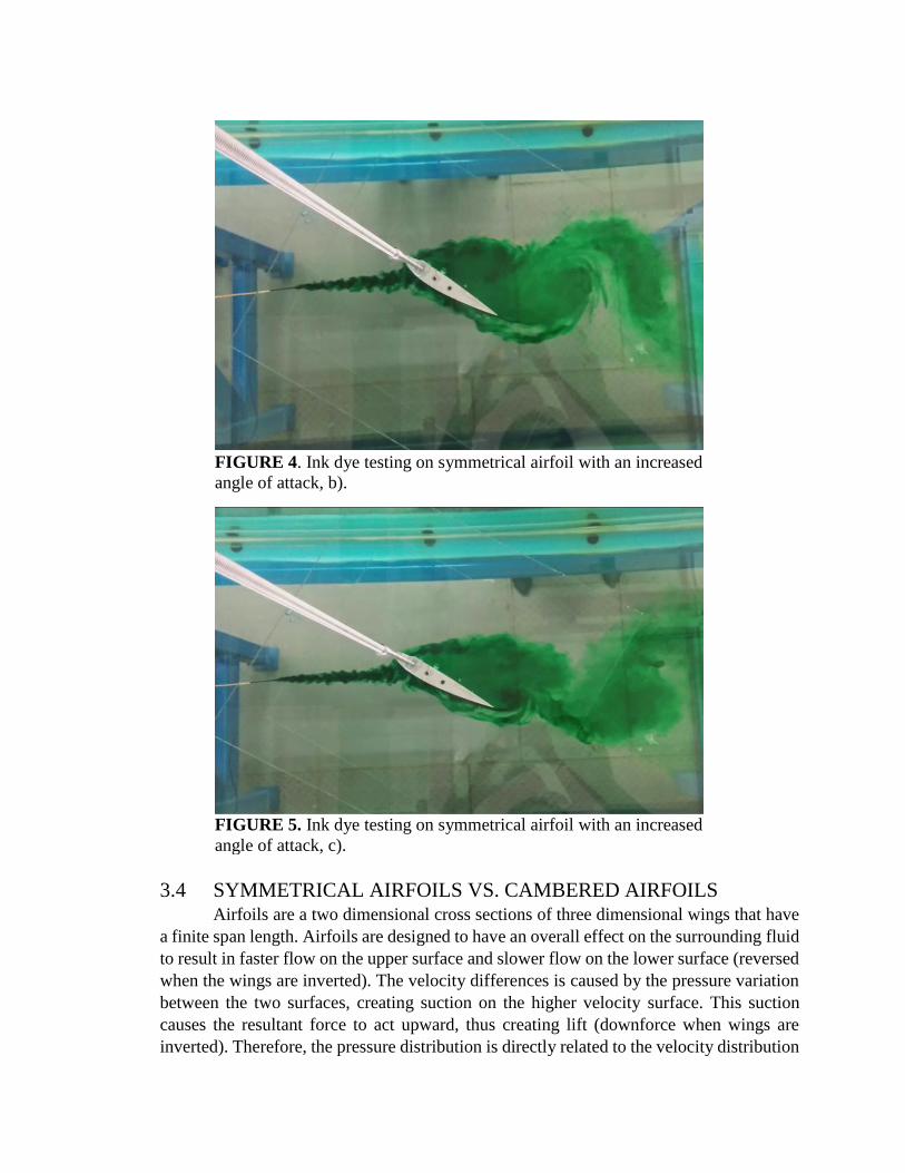
3.4 SYMMETRICAL AIRFOILS VS. CAMBERED AIRFOILS Airfoils are a two dimensional cross sections of three dimensional wings that have

a finite span length. Airfoils are designed to have an overall effect on the surrounding fluid

to result in faster flow on the upper surface and slower flow on the lower surface (reversed

when the wings are inverted). The velocity differences is caused by the pressure variation

between the two surfaces, creating suction on the higher velocity surface. This suction

causes the resultant force to act upward, thus creating lift (downforce when wings are

inverted). Therefore, the pressure distribution is directly related to the velocity distribution

FIGURE 4. Ink dye testing on symmetrical airfoil with an increased

angle of attack, b).

FIGURE 5. Ink dye testing on symmetrical airfoil with an increased

angle of attack, c).

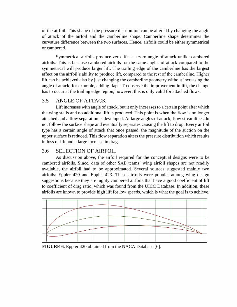
of the airfoil. This shape of the pressure distribution can be altered by changing the angle

of attack of the airfoil and the camberline shape. Camberline shape determines the

curvature difference between the two surfaces. Hence, airfoils could be either symmetrical

or cambered.

Symmetrical airfoils produce zero lift at a zero angle of attack unlike cambered

airfoils. This is because cambered airfoils for the same angles of attack compared to the

symmetrical will produce larger lift. The trailing edge of the camberline has the largest

effect on the airfoil’s ability to produce lift, compared to the rest of the camberline. Higher

lift can be achieved also by just changing the camberline geometry without increasing the

angle of attack; for example, adding flaps. To observe the improvement in lift, the change

has to occur at the trailing edge region, however, this is only valid for attached flows.

3.5 ANGLE OF ATTACK Lift increases with angle of attack, but it only increases to a certain point after which

the wing stalls and no additional lift is produced. This point is when the flow is no longer

attached and a flow separation is developed. At large angles of attack, flow streamlines do

not follow the surface shape and eventually separates causing the lift to drop. Every airfoil

type has a certain angle of attack that once passed, the magnitude of the suction on the

upper surface is reduced. This flow separation alters the pressure distribution which results

in loss of lift and a large increase in drag.

3.6 SELECTION OF AIRFOIL As discussion above, the airfoil required for the conceptual designs were to be

cambered airfoils. Since, data of other SAE teams’ wing airfoil shapes are not readily

available, the airfoil had to be approximated. Several sources suggested mainly two

airfoils: Eppler 420 and Eppler 423. These airfoils were popular among wing design

suggestions because they are highly cambered airfoils that have a good coefficient of lift

to coefficient of drag ratio, which was found from the UICC Database. In addition, these

airfoils are known to provide high lift for low speeds, which is what the goal is to achieve.

FIGURE 6. Eppler 420 obtained from the NACA Database [6].

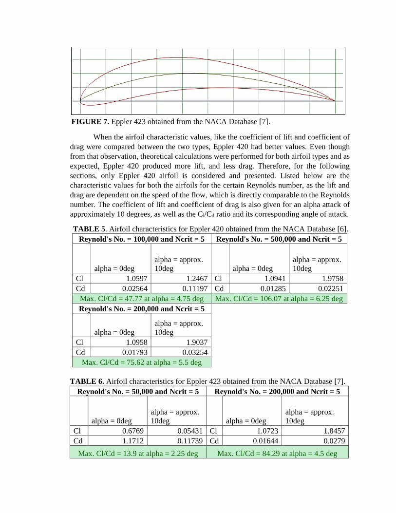
When the airfoil characteristic values, like the coefficient of lift and coefficient of

drag were compared between the two types, Eppler 420 had better values. Even though

from that observation, theoretical calculations were performed for both airfoil types and as

expected, Eppler 420 produced more lift, and less drag. Therefore, for the following

sections, only Eppler 420 airfoil is considered and presented. Listed below are the

characteristic values for both the airfoils for the certain Reynolds number, as the lift and

drag are dependent on the speed of the flow, which is directly comparable to the Reynolds

number. The coefficient of lift and coefficient of drag is also given for an alpha attack of

approximately 10 degrees, as well as the Cl/Cd ratio and its corresponding angle of attack.

TABLE 5. Airfoil characteristics for Eppler 420 obtained from the NACA Database [6].

Reynold's No. = 100,000 and Ncrit = 5 Reynold's No. = 500,000 and Ncrit = 5

alpha = 0deg

alpha = approx.

10deg alpha = 0deg

alpha = approx.

10deg

Cl 1.0597 1.2467 Cl 1.0941 1.9758

Cd 0.02564 0.11197 Cd 0.01285 0.02251

Max. Cl/Cd = 47.77 at alpha = 4.75 deg Max. Cl/Cd = 106.07 at alpha = 6.25 deg

Reynold's No. = 200,000 and Ncrit = 5

alpha = 0deg

alpha = approx.

10deg

Cl 1.0958 1.9037

Cd 0.01793 0.03254

Max. Cl/Cd = 75.62 at alpha = 5.5 deg

TABLE 6. Airfoil characteristics for Eppler 423 obtained from the NACA Database [7].

Reynold's No. = 50,000 and Ncrit = 5 Reynold's No. = 200,000 and Ncrit = 5

alpha = 0deg

alpha = approx.

10deg alpha = 0deg

alpha = approx.

10deg

Cl 0.6769 0.05431 Cl 1.0723 1.8457

Cd 1.1712 0.11739 Cd 0.01644 0.0279

Max. Cl/Cd = 13.9 at alpha = 2.25 deg Max. Cl/Cd = 84.29 at alpha = 4.5 deg

FIGURE 7. Eppler 423 obtained from the NACA Database [7].

Reynold's No. = 100,000 and Ncrit = 5 Reynold's No. = 500,000 and Ncrit = 5

alpha = 0deg

alpha = approx.

10deg alpha = 0deg

alpha = approx.

10deg

Cl 1.0177 1.5567 Cl 1.074 1.8885

Cd 0.02408 0.05731 Cd 0.01158 0.02153

Max. Cl/Cd = 51.9 at alpha = 4.25 deg Max. Cl/Cd = 120.55 at alpha = 5.5 deg

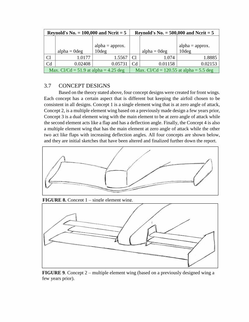
3.7 CONCEPT DESIGNS Based on the theory stated above, four concept designs were created for front wings.

Each concept has a certain aspect that is different but keeping the airfoil chosen to be

consistent in all designs. Concept 1 is a single element wing that is at zero angle of attack,

Concept 2, is a multiple element wing based on a previously made design a few years prior,

Concept 3 is a dual element wing with the main element to be at zero angle of attack while

the second element acts like a flap and has a deflection angle. Finally, the Concept 4 is also

a multiple element wing that has the main element at zero angle of attack while the other

two act like flaps with increasing deflection angles. All four concepts are shown below,

and they are initial sketches that have been altered and finalized further down the report.

FIGURE 8. Concept 1 – single element wing.

FIGURE 9. Concept 2 – multiple element wing (based on a previously designed wing a

few years prior).

The reason why the concepts have a variation of number of elements is because

having a multiple element wing is proven to be more effective than single element wings.

Theoretically, they generate more downforce because of the suction that’s created due to

the slot gaps between the elements which also leads to a more attached flow. Like

previously mentioned, without increasing the angle of attack, higher lift can be achieved

by altering the trailing edge flow behaviour through the addition of flaps. Therefore, the

concepts include a single and multiple elements design in order to prove this theory through

theoretical calculations and experimental testing. Another reason why single element wing

is less efficient is because of the single large vortex that would be produced by the wing.

This large vortex is considered powerful and is pointed outwards to a smaller area

downstream on the car. Having multiple element wing, the vortex can be split into separate

sections creating several smaller vortices. These smaller vortices are lower in energy and

will be spread over a wider area. Vortices are extremely high energy structures that can

negatively affect the performance of the wing, unless vortex generators are positioned

correctly for it to have a positive effect. If positioned correctly, the vortices created can

keep the high pressure air around the car from entering the low pressure underbody region

which leads to maintaining the downforce created by the wings. These theories have to be

proven experimentally once a model of the wings are tested in the wind tunnel [2].

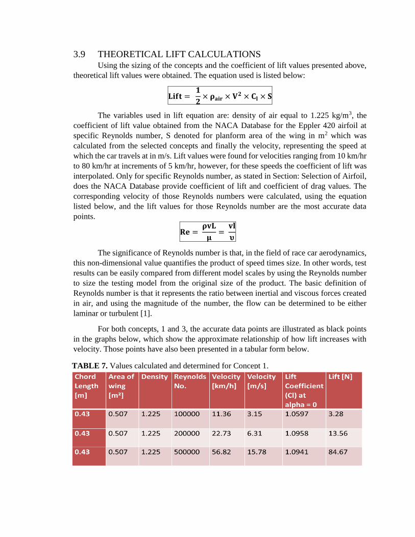
3.8 SIZING Among the four concepts presented in the previous section, only two concepts were

chosen to move forward to sizing and 3-D modelling for performing theoretical

calculations. The concepts that were chosen were Concept 1 and Concept 3 and the design

has been altered to be a bit different, as illustrated in the figures below. The concepts have

FIGURE 10. Concept 3 – dual element wing.

FIGURE 11. Concept 4 – multiple element wing (main element and 2 flaps).

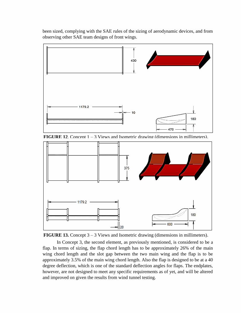
been sized, complying with the SAE rules of the sizing of aerodynamic devices, and from

observing other SAE team designs of front wings.

In Concept 3, the second element, as previously mentioned, is considered to be a

flap. In terms of sizing, the flap chord length has to be approximately 26% of the main

wing chord length and the slot gap between the two main wing and the flap is to be

approximately 3.5% of the main wing chord length. Also the flap is designed to be at a 40

degree deflection, which is one of the standard deflection angles for flaps. The endplates,

however, are not designed to meet any specific requirements as of yet, and will be altered

and improved on given the results from wind tunnel testing.

FIGURE 12. Concept 1 – 3 Views and Isometric drawing (dimensions in millimeters).

FIGURE 13. Concept 3 – 3 Views and Isometric drawing (dimensions in millimeters).

3.9 THEORETICAL LIFT CALCULATIONS Using the sizing of the concepts and the coefficient of lift values presented above,

theoretical lift values were obtained. The equation used is listed below:

𝐋𝐢𝐟𝐭 = 𝟏

𝟐× 𝛒𝐚𝐢𝐫 × 𝐕𝟐 × 𝐂𝐥 × 𝐒

The variables used in lift equation are: density of air equal to 1.225 kg/m3, the

coefficient of lift value obtained from the NACA Database for the Eppler 420 airfoil at

specific Reynolds number, S denoted for planform area of the wing in m2 which was

calculated from the selected concepts and finally the velocity, representing the speed at

which the car travels at in m/s. Lift values were found for velocities ranging from 10 km/hr

to 80 km/hr at increments of 5 km/hr, however, for these speeds the coefficient of lift was

interpolated. Only for specific Reynolds number, as stated in Section: Selection of Airfoil,

does the NACA Database provide coefficient of lift and coefficient of drag values. The

corresponding velocity of those Reynolds numbers were calculated, using the equation

listed below, and the lift values for those Reynolds number are the most accurate data

points.

𝐑𝐞 = 𝛒𝐯𝐋

𝛍=

𝐯𝐥

𝛖

The significance of Reynolds number is that, in the field of race car aerodynamics,

this non-dimensional value quantifies the product of speed times size. In other words, test

results can be easily compared from different model scales by using the Reynolds number

to size the testing model from the original size of the product. The basic definition of

Reynolds number is that it represents the ratio between inertial and viscous forces created

in air, and using the magnitude of the number, the flow can be determined to be either

laminar or turbulent [1].

For both concepts, 1 and 3, the accurate data points are illustrated as black points

in the graphs below, which show the approximate relationship of how lift increases with

velocity. Those points have also been presented in a tabular form below.

TABLE 7. Values calculated and determined for Concept 1.

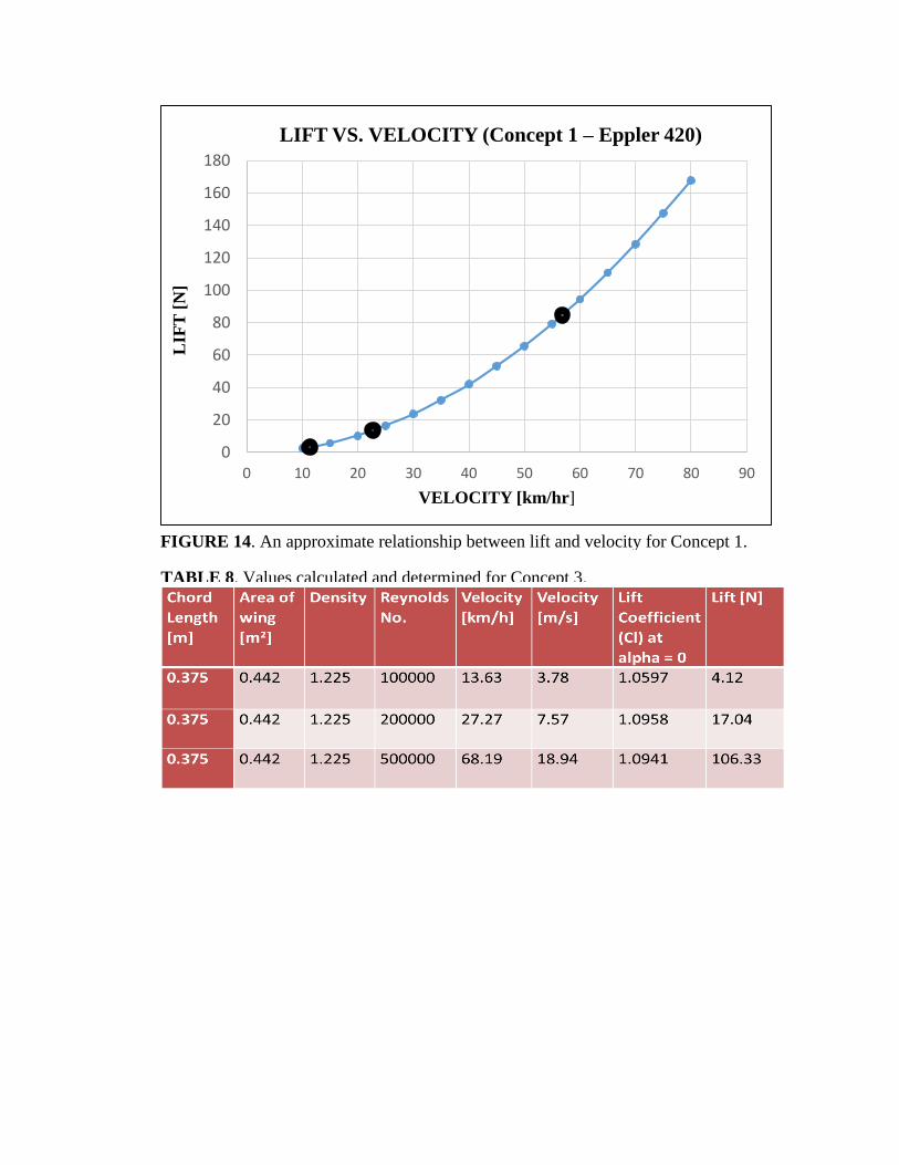
TABLE 8. Values calculated and determined for Concept 3.

0

20

40

60

80

100

120

140

160

180

0 10 20 30 40 50 60 70 80 90

LIF

T [

N]

VELOCITY [km/hr]

LIFT VS. VELOCITY (Concept 1 – Eppler 420)

FIGURE 14. An approximate relationship between lift and velocity for Concept 1.

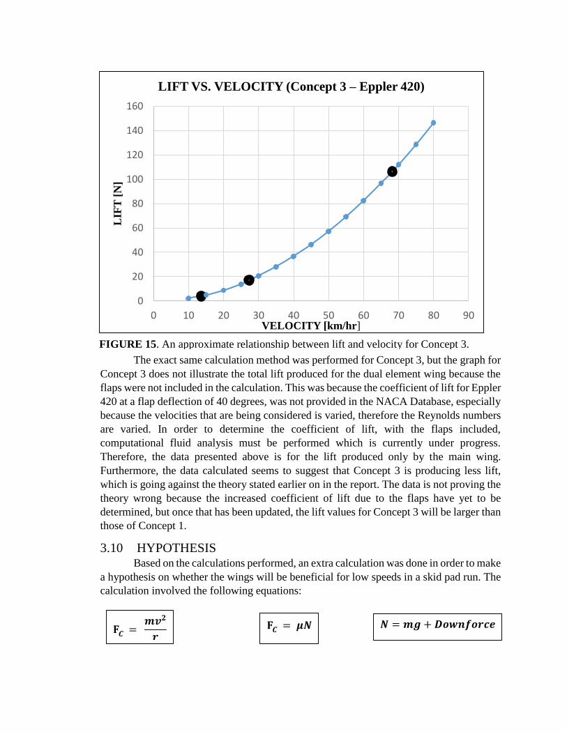
The exact same calculation method was performed for Concept 3, but the graph for

Concept 3 does not illustrate the total lift produced for the dual element wing because the

flaps were not included in the calculation. This was because the coefficient of lift for Eppler

420 at a flap deflection of 40 degrees, was not provided in the NACA Database, especially

because the velocities that are being considered is varied, therefore the Reynolds numbers

are varied. In order to determine the coefficient of lift, with the flaps included,

computational fluid analysis must be performed which is currently under progress.

Therefore, the data presented above is for the lift produced only by the main wing.

Furthermore, the data calculated seems to suggest that Concept 3 is producing less lift,

which is going against the theory stated earlier on in the report. The data is not proving the

theory wrong because the increased coefficient of lift due to the flaps have yet to be

determined, but once that has been updated, the lift values for Concept 3 will be larger than

those of Concept 1.

3.10 HYPOTHESIS Based on the calculations performed, an extra calculation was done in order to make

a hypothesis on whether the wings will be beneficial for low speeds in a skid pad run. The

calculation involved the following equations:

𝐅𝑪 = 𝒎𝒗𝟐

𝒓 𝐅𝑪 = 𝝁𝑵 𝑵 = 𝒎𝒈 + 𝑫𝒐𝒘𝒏𝒇𝒐𝒓𝒄𝒆

0

20

40

60

80

100

120

140

160

0 10 20 30 40 50 60 70 80 90

LIF

T [

N]

VELOCITY [km/hr]

LIFT VS. VELOCITY (Concept 3 – Eppler 420)

FIGURE 15. An approximate relationship between lift and velocity for Concept 3.

The variables stated above represent: Fc is the centrifugal force present on the car

when it turns in a skid pad track, m is the mass of the car, r is the radius of the skid pad, 𝜇

is the friction coefficient and N represents the normal force active on the car. The normal

force for a car without wings is just the weight of the car, but with the addition of wings,

the normal force then equals the weight of the car plus the downforce generated by the

wings. In order effectively do this calculation, there are couple of assumptions that had to

be made. When performing the calculation, it is being assumed that the wing is placed at

an optimal position on the car. Optimal position suggests that the wing gets maximum

undisturbed and clean airflow (an example of a position would be placing the wing near

the roll hoop of the car). Which this placement of the wing, it is also assumed that the

downforce produced will be equally distributed between the front and rear axle.

Given those assumptions and considering the car as point in a free body diagram,

the calculation is performed. So, for an arbitrary downforce of 84.67 N, which is

approximately 8 kg in mass, the car would have to be traveling at a speed of 56.82 km/hr

(values corresponding to 500 000 Reynolds for Concept 1). To maintain this speed around

a skid pad, without sliding and understeer, provided that the mass of the car is 435 lbs and

the coefficient of friction is equal to one, the radius of curvature of the skid pad needs to

be 25.38 m. Analyzing this exact scenario but with the Concept 1 wing and the assumptions

stated earlier, the calculation yields a speed value of only 58.03 km/hr around the skid pad.

This shows that the change in speed around a skid pad when a wing is included is not very

significant. Also, this increase in speed is the highest theoretical speed that can be achieved,

but in a real life situation there are several factors that would not allow this increase and

could potentially even eliminate this improvement. Although, the 2 km/hr increase in speed

might look significant, for the competition the skid pad radius is only 8 m. This would

mean the speed at which the car travels into the skid pad would be much slower, leading

to lower downforce created, finally resulting in a difference in velocity to be far less.

Therefore, at this stage of the design process and with the data in hand, the hypothesis

being made of the usefulness of wings at low speeds is negligible, when compared to the

drag and weight consequences the wing will have on the car.

3.11 COAST DOWN TESTING The purpose of conducting a coast down testing using the RR14, is to determine

the drag effects that are currently on the car. The test is performed by driving the vehicle

to max. speed at which the traction force will be removed and the vehicle will be let to

coast freely until the velocity reduces to a zero or a specific defined value. During the test,

the velocity over time is recorded and through those values, the drag characteristics can be

found. The drag is related to the time rate of change of linear momentum. The test must be

performed several times under the same conditions in order to achieve an adequate level of

statistical confidence on the results. Instead of measuring the velocity over time, the

acceleration over time could be recorded or even the displacement of the car over time can

be used. The advantage of using acceleration is that it simplifies the analysis procedure as

acceleration can be easily applied to the following differential equation [8]:

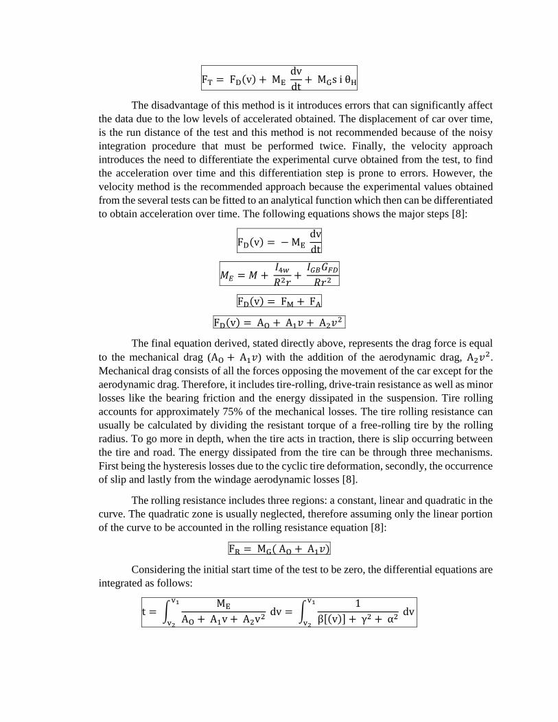
FT = FD(v) + ME dv

dt+ MGs i θH

The disadvantage of this method is it introduces errors that can significantly affect

the data due to the low levels of accelerated obtained. The displacement of car over time,

is the run distance of the test and this method is not recommended because of the noisy

integration procedure that must be performed twice. Finally, the velocity approach

introduces the need to differentiate the experimental curve obtained from the test, to find

the acceleration over time and this differentiation step is prone to errors. However, the

velocity method is the recommended approach because the experimental values obtained

from the several tests can be fitted to an analytical function which then can be differentiated

to obtain acceleration over time. The following equations shows the major steps [8]:

FD(v) = − ME dv

dt

𝑀𝐸 = 𝑀 + 𝐼4𝑤

𝑅2𝑟+

𝐼𝐺𝐵𝐺𝐹𝐷

𝑅𝑟2

FD(v) = FM + FA

FD(v) = AO + A1𝑣 + A2𝑣2

The final equation derived, stated directly above, represents the drag force is equal

to the mechanical drag (AO + A1𝑣) with the addition of the aerodynamic drag, A2𝑣2.

Mechanical drag consists of all the forces opposing the movement of the car except for the

aerodynamic drag. Therefore, it includes tire-rolling, drive-train resistance as well as minor

losses like the bearing friction and the energy dissipated in the suspension. Tire rolling

accounts for approximately 75% of the mechanical losses. The tire rolling resistance can

usually be calculated by dividing the resistant torque of a free-rolling tire by the rolling

radius. To go more in depth, when the tire acts in traction, there is slip occurring between

the tire and road. The energy dissipated from the tire can be through three mechanisms.

First being the hysteresis losses due to the cyclic tire deformation, secondly, the occurrence

of slip and lastly from the windage aerodynamic losses [8].

The rolling resistance includes three regions: a constant, linear and quadratic in the

curve. The quadratic zone is usually neglected, therefore assuming only the linear portion

of the curve to be accounted in the rolling resistance equation [8]:

FR = MG( AO + A1𝑣)

Considering the initial start time of the test to be zero, the differential equations are

integrated as follows:

t = ∫ME

AO + A1v + A2v2

v1

v2

dv = ∫1

β[(v)] + γ2 + α2

v1

v2

dv

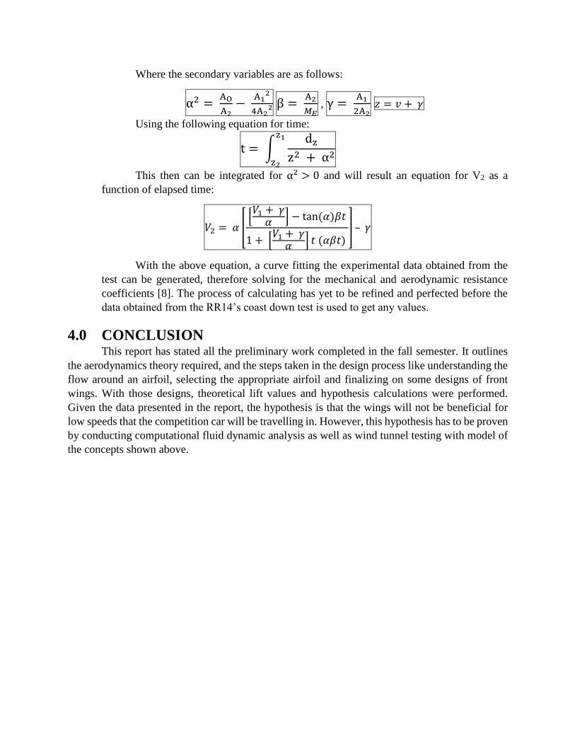
Where the secondary variables are as follows:

α2 = AO

A2−

A12

4A22 β =

A2

𝑀𝐸 , γ =

A1

2A2 𝑧 = 𝑣 + 𝛾

Using the following equation for time:

t = ∫dz

z2 + α2

z1

z2

This then can be integrated for α2 > 0 and will result an equation for V2 as a

function of elapsed time:

𝑉2 = 𝛼 [[𝑉1 + 𝛾

𝛼 ] − tan (𝛼)𝛽𝑡

1 + [𝑉1 + 𝛾

𝛼 ] 𝑡 (𝛼𝛽𝑡) ] – 𝛾

With the above equation, a curve fitting the experimental data obtained from the

test can be generated, therefore solving for the mechanical and aerodynamic resistance

coefficients [8]. The process of calculating has yet to be refined and perfected before the

data obtained from the RR14’s coast down test is used to get any values.

4.0 CONCLUSION This report has stated all the preliminary work completed in the fall semester. It outlines

the aerodynamics theory required, and the steps taken in the design process like understanding the

flow around an airfoil, selecting the appropriate airfoil and finalizing on some designs of front

wings. With those designs, theoretical lift values and hypothesis calculations were performed.

Given the data presented in the report, the hypothesis is that the wings will not be beneficial for

low speeds that the competition car will be travelling in. However, this hypothesis has to be proven

by conducting computational fluid dynamic analysis as well as wind tunnel testing with model of

the concepts shown above.

5.0 REFERENCES

[1] J. Katz, in Race Car Aerodynamics, Cambridge, Bentley Publishers, 2004.

[2] "Formula1 Dictionary," 2012. [Online]. Available: http://www.formula1-

dictionary.net/f_w_endplate.html. [Accessed 28 September 2014].

[3] C. Kirk, "Badger GP," 30 March 2012. [Online]. Available:

http://badgergp.com/2012/03/badger-gp-gives-you-front-wings/. [Accessed 28

September 2014].

[4] "Formula1 Dictionary," 2012. [Online]. Available: http://www.formula1-

dictionary.net/flow_viz_paint.html. [Accessed 28 Septmeber 2014].

[5] Gray, "Automotive Aerodynamics," Youtube, 30 September 2014. [Online]. Available:

https://www.youtube.com/watch?v=quDLzxmJl5I. [Accessed 19 October 2014].

[6] "Airfoil Tools," 2014. [Online]. Available:

http://airfoiltools.com/airfoil/details?airfoil=e420-il. [Accessed November 2014].

[7] "Airfoil Tools," 2014. [Online]. Available:

http://airfoiltools.com/airfoil/details?airfoil=e423-il. [Accessed November 2014].

[8] Z. T. Cai, J. J. Worm and D. D. Brennan, "Experimental Studies in Ground Vehicle

Coast-Down Testing," American Society for Engineering Education, 2012.

PART 2 – WINTER SEMESTER

1.0 INTRODUCTION What was accomplished in the fall semester, as previously stated in the report, was the

theory behind the flow around an airfoil depending on its profile shape, 3D rendering of front wing

designs and theoretical lift calculations for those designs. This semester some of the values used

for the theoretical calculations are supported by performing computational analysis using XFOIL

and conducting wind tunnel testing to obtain experimental data. Two concepts of front wings were

3D printed for the wind tunnel testing to determine if the wing produced any downforce. The

models that were printed was a single element front wing and a multiple element front wing that

includes two flaps. In addition, computational analysis was conducted using Workbench ANYSYS

to determine velocity, pressure and force contours for the multiple element wing design, as well

as the airflow simulation over the wing. Finally, a few concept sketches were created to start the

design process for a more complex and beneficial endplate, rather than a simple piece that used

for testing purposes. Therefore, Part 2 of this report will mainly focus on presenting results

obtained.

2.0 XFOIL XFOIL is a program that is written in FORTRAN and is used to analyse subsonic isolated

airfoils given the coordinates detailing the shape of the airfoil profile, the Reynolds and Mach

numbers [1]. The program then calculates the pressure distribution that is occurring under those

conditions which then leads to finding the airfoil’s lift and drag characteristics [1].

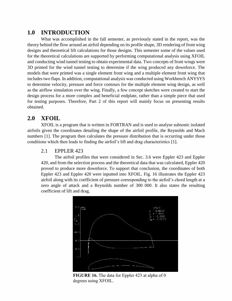
2.1 EPPLER 423 The airfoil profiles that were considered in Sec. 3.6 were Eppler 423 and Eppler

420, and from the selection process and the theoretical data that was calculated, Eppler 420

proved to produce more downforce. To support that conclusion, the coordinates of both

Eppler 423 and Eppler 420 were inputted into XFOIL. Fig. 16 illustrates the Eppler 423

airfoil along with its coefficient of pressure corresponding to the airfoil’s chord length at a

zero angle of attack and a Reynolds number of 300 000. It also states the resulting

coefficient of lift and drag.

FIGURE 16. The data for Eppler 423 at alpha of 0

degrees using XFOIL.

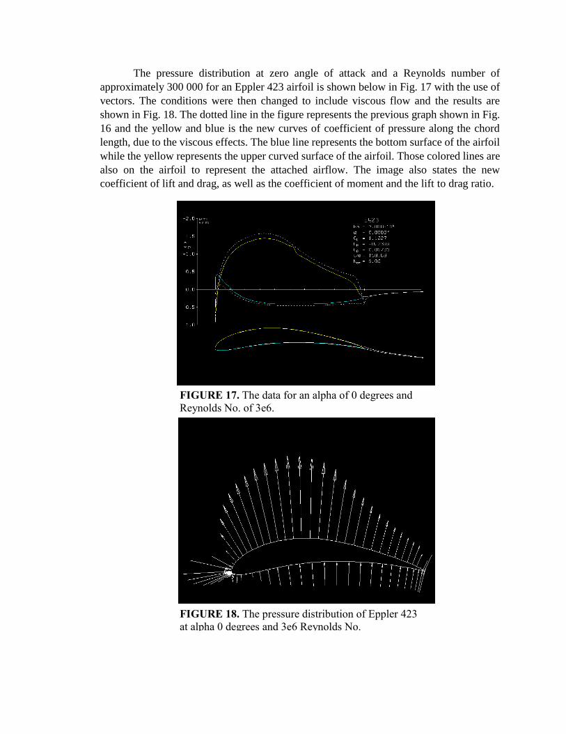
The pressure distribution at zero angle of attack and a Reynolds number of

approximately 300 000 for an Eppler 423 airfoil is shown below in Fig. 17 with the use of

vectors. The conditions were then changed to include viscous flow and the results are

shown in Fig. 18. The dotted line in the figure represents the previous graph shown in Fig.

16 and the yellow and blue is the new curves of coefficient of pressure along the chord

length, due to the viscous effects. The blue line represents the bottom surface of the airfoil

while the yellow represents the upper curved surface of the airfoil. Those colored lines are

also on the airfoil to represent the attached airflow. The image also states the new

coefficient of lift and drag, as well as the coefficient of moment and the lift to drag ratio.

FIGURE 17. The data for an alpha of 0 degrees and

Reynolds No. of 3e6.

FIGURE 18. The pressure distribution of Eppler 423

at alpha 0 degrees and 3e6 Reynolds No.

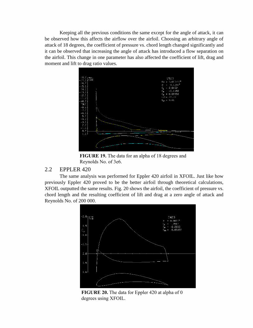
Keeping all the previous conditions the same except for the angle of attack, it can

be observed how this affects the airflow over the airfoil. Choosing an arbitrary angle of

attack of 18 degrees, the coefficient of pressure vs. chord length changed significantly and

it can be observed that increasing the angle of attack has introduced a flow separation on

the airfoil. This change in one parameter has also affected the coefficient of lift, drag and

moment and lift to drag ratio values.

2.2 EPPLER 420 The same analysis was performed for Eppler 420 airfoil in XFOIL. Just like how

previously Eppler 420 proved to be the better airfoil through theoretical calculations,

XFOIL outputted the same results. Fig. 20 shows the airfoil, the coefficient of pressure vs.

chord length and the resulting coefficient of lift and drag at a zero angle of attack and

Reynolds No. of 200 000.

FIGURE 19. The data for an alpha of 18 degrees and

Reynolds No. of 3e6.

FIGURE 20. The data for Eppler 420 at alpha of 0

degrees using XFOIL.

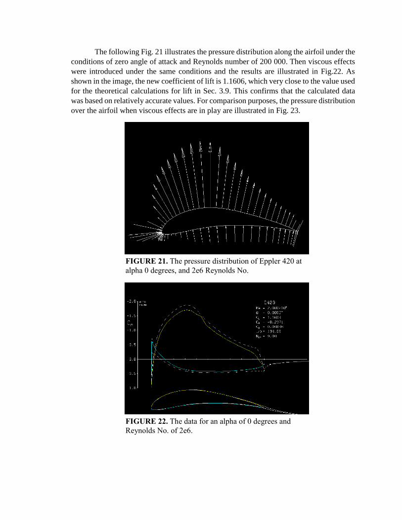
The following Fig. 21 illustrates the pressure distribution along the airfoil under the

conditions of zero angle of attack and Reynolds number of 200 000. Then viscous effects

were introduced under the same conditions and the results are illustrated in Fig.22. As

shown in the image, the new coefficient of lift is 1.1606, which very close to the value used

for the theoretical calculations for lift in Sec. 3.9. This confirms that the calculated data

was based on relatively accurate values. For comparison purposes, the pressure distribution

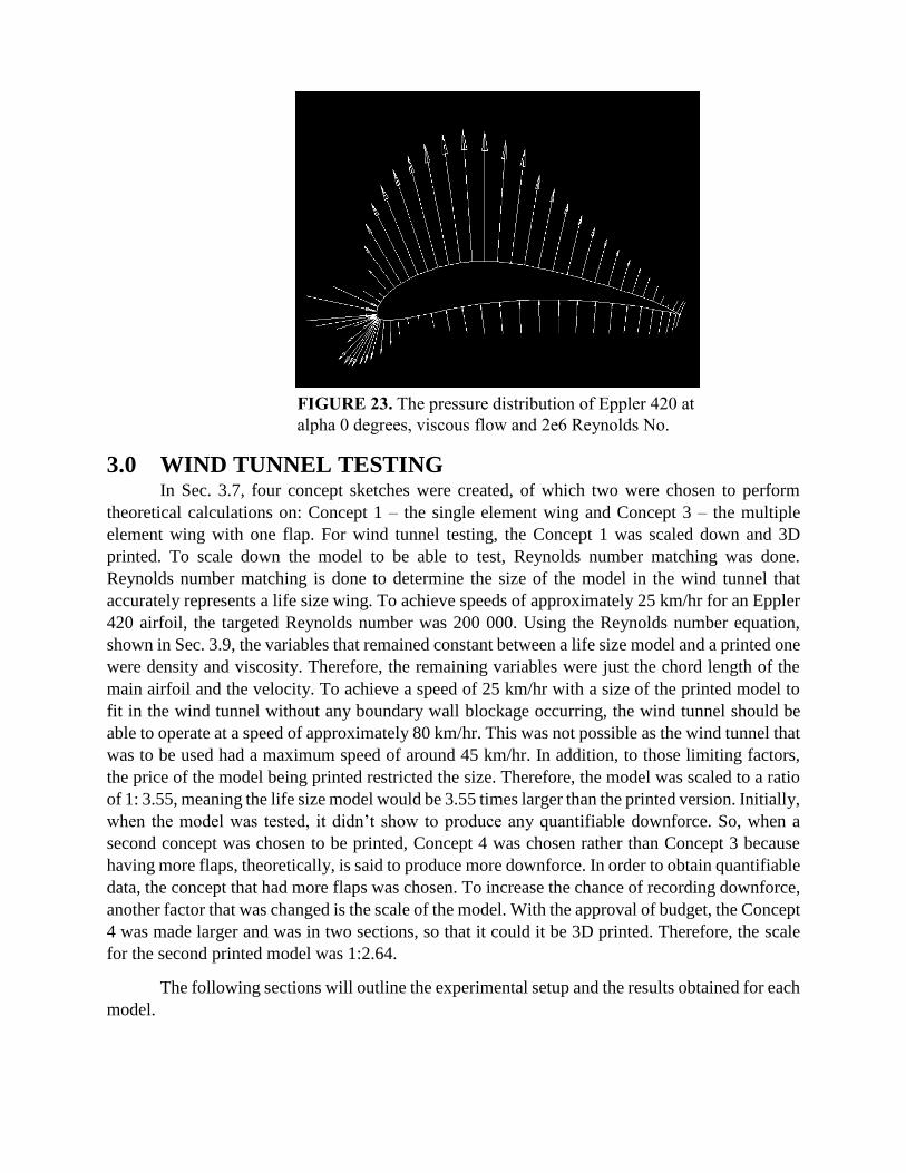
over the airfoil when viscous effects are in play are illustrated in Fig. 23.

FIGURE 21. The pressure distribution of Eppler 420 at

alpha 0 degrees, and 2e6 Reynolds No.

FIGURE 22. The data for an alpha of 0 degrees and

Reynolds No. of 2e6.

3.0 WIND TUNNEL TESTING In Sec. 3.7, four concept sketches were created, of which two were chosen to perform

theoretical calculations on: Concept 1 – the single element wing and Concept 3 – the multiple

element wing with one flap. For wind tunnel testing, the Concept 1 was scaled down and 3D

printed. To scale down the model to be able to test, Reynolds number matching was done.

Reynolds number matching is done to determine the size of the model in the wind tunnel that

accurately represents a life size wing. To achieve speeds of approximately 25 km/hr for an Eppler

420 airfoil, the targeted Reynolds number was 200 000. Using the Reynolds number equation,

shown in Sec. 3.9, the variables that remained constant between a life size model and a printed one

were density and viscosity. Therefore, the remaining variables were just the chord length of the

main airfoil and the velocity. To achieve a speed of 25 km/hr with a size of the printed model to

fit in the wind tunnel without any boundary wall blockage occurring, the wind tunnel should be

able to operate at a speed of approximately 80 km/hr. This was not possible as the wind tunnel that

was to be used had a maximum speed of around 45 km/hr. In addition, to those limiting factors,

the price of the model being printed restricted the size. Therefore, the model was scaled to a ratio

of 1: 3.55, meaning the life size model would be 3.55 times larger than the printed version. Initially,

when the model was tested, it didn’t show to produce any quantifiable downforce. So, when a

second concept was chosen to be printed, Concept 4 was chosen rather than Concept 3 because

having more flaps, theoretically, is said to produce more downforce. In order to obtain quantifiable

data, the concept that had more flaps was chosen. To increase the chance of recording downforce,

another factor that was changed is the scale of the model. With the approval of budget, the Concept

4 was made larger and was in two sections, so that it could it be 3D printed. Therefore, the scale

for the second printed model was 1:2.64.

The following sections will outline the experimental setup and the results obtained for each

model.

FIGURE 23. The pressure distribution of Eppler 420 at

alpha 0 degrees, viscous flow and 2e6 Reynolds No.

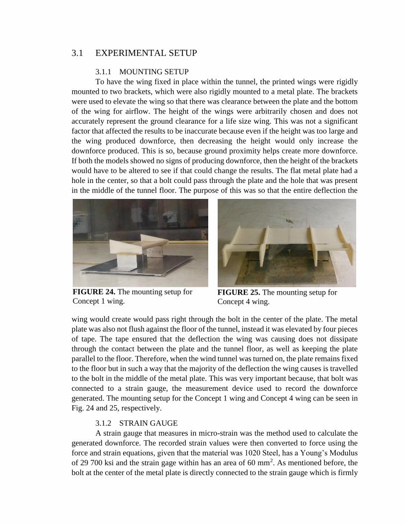
3.1 EXPERIMENTAL SETUP

3.1.1 MOUNTING SETUP

To have the wing fixed in place within the tunnel, the printed wings were rigidly

mounted to two brackets, which were also rigidly mounted to a metal plate. The brackets

were used to elevate the wing so that there was clearance between the plate and the bottom

of the wing for airflow. The height of the wings were arbitrarily chosen and does not

accurately represent the ground clearance for a life size wing. This was not a significant

factor that affected the results to be inaccurate because even if the height was too large and

the wing produced downforce, then decreasing the height would only increase the

downforce produced. This is so, because ground proximity helps create more downforce.

If both the models showed no signs of producing downforce, then the height of the brackets

would have to be altered to see if that could change the results. The flat metal plate had a

hole in the center, so that a bolt could pass through the plate and the hole that was present

in the middle of the tunnel floor. The purpose of this was so that the entire deflection the

wing would create would pass right through the bolt in the center of the plate. The metal

plate was also not flush against the floor of the tunnel, instead it was elevated by four pieces

of tape. The tape ensured that the deflection the wing was causing does not dissipate

through the contact between the plate and the tunnel floor, as well as keeping the plate

parallel to the floor. Therefore, when the wind tunnel was turned on, the plate remains fixed

to the floor but in such a way that the majority of the deflection the wing causes is travelled

to the bolt in the middle of the metal plate. This was very important because, that bolt was

connected to a strain gauge, the measurement device used to record the downforce

generated. The mounting setup for the Concept 1 wing and Concept 4 wing can be seen in

Fig. 24 and 25, respectively.

3.1.2 STRAIN GAUGE

A strain gauge that measures in micro-strain was the method used to calculate the

generated downforce. The recorded strain values were then converted to force using the

force and strain equations, given that the material was 1020 Steel, has a Young’s Modulus

of 29 700 ksi and the strain gage within has an area of 60 mm2. As mentioned before, the

bolt at the center of the metal plate is directly connected to the strain gauge which is firmly

FIGURE 24. The mounting setup for

Concept 1 wing. FIGURE 25. The mounting setup for

Concept 4 wing.

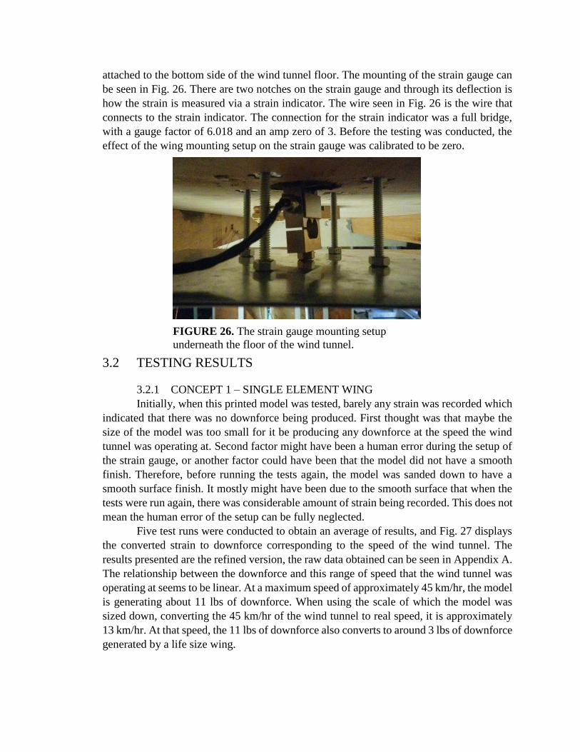
attached to the bottom side of the wind tunnel floor. The mounting of the strain gauge can

be seen in Fig. 26. There are two notches on the strain gauge and through its deflection is

how the strain is measured via a strain indicator. The wire seen in Fig. 26 is the wire that

connects to the strain indicator. The connection for the strain indicator was a full bridge,

with a gauge factor of 6.018 and an amp zero of 3. Before the testing was conducted, the

effect of the wing mounting setup on the strain gauge was calibrated to be zero.

3.2 TESTING RESULTS

3.2.1 CONCEPT 1 – SINGLE ELEMENT WING

Initially, when this printed model was tested, barely any strain was recorded which

indicated that there was no downforce being produced. First thought was that maybe the

size of the model was too small for it be producing any downforce at the speed the wind

tunnel was operating at. Second factor might have been a human error during the setup of

the strain gauge, or another factor could have been that the model did not have a smooth

finish. Therefore, before running the tests again, the model was sanded down to have a

smooth surface finish. It mostly might have been due to the smooth surface that when the

tests were run again, there was considerable amount of strain being recorded. This does not

mean the human error of the setup can be fully neglected.

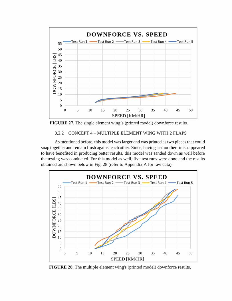
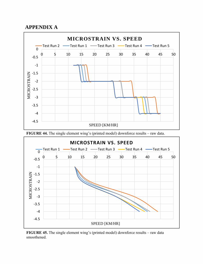
Five test runs were conducted to obtain an average of results, and Fig. 27 displays

the converted strain to downforce corresponding to the speed of the wind tunnel. The

results presented are the refined version, the raw data obtained can be seen in Appendix A.

The relationship between the downforce and this range of speed that the wind tunnel was

operating at seems to be linear. At a maximum speed of approximately 45 km/hr, the model

is generating about 11 lbs of downforce. When using the scale of which the model was

sized down, converting the 45 km/hr of the wind tunnel to real speed, it is approximately

13 km/hr. At that speed, the 11 lbs of downforce also converts to around 3 lbs of downforce

generated by a life size wing.

FIGURE 26. The strain gauge mounting setup

underneath the floor of the wind tunnel.

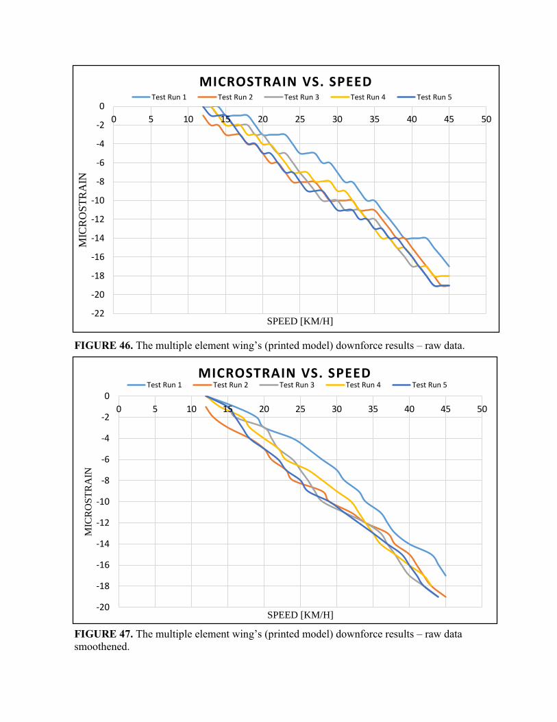
3.2.2 CONCEPT 4 – MULTIPLE ELEMENT WING WITH 2 FLAPS

As mentioned before, this model was larger and was printed as two pieces that could

snap together and remain flush against each other. Since, having a smoother finish appeared

to have benefited in producing better results, this model was sanded down as well before

the testing was conducted. For this model as well, five test runs were done and the results

obtained are shown below in Fig. 28 (refer to Appendix A for raw data).

FIGURE 27. The single element wing’s (printed model) downforce results.

0

5

10

15

20

25

30

35

40

45

50

55

0 5 10 15 20 25 30 35 40 45 50

DO

WN

FO

RC

E [

LB

S]

SPEED [KM/HR]

DOWNFORCE VS. SPEEDTest Run 1 Test Run 2 Test Run 3 Test Run 4 Test Run 5

0

5

10

15

20

25

30

35

40

45

50

55

0 5 10 15 20 25 30 35 40 45 50

DO

WN

FO

RC

E [

LB

S]

SPEED [KM/HR]

DOWNFORCE VS. SPEEDTest Run 1 Test Run 2 Test Run 3 Test Run 4 Test Run 5

FIGURE 28. The multiple element wing's (printed model) downforce results.

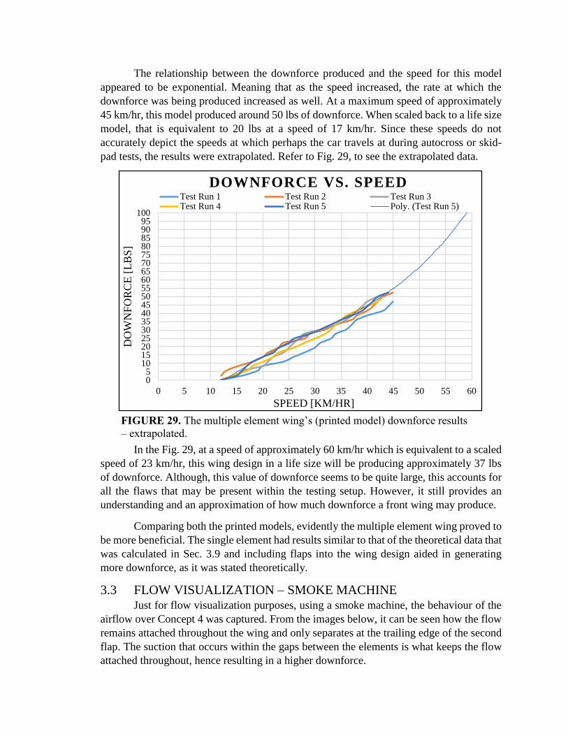
The relationship between the downforce produced and the speed for this model

appeared to be exponential. Meaning that as the speed increased, the rate at which the

downforce was being produced increased as well. At a maximum speed of approximately

45 km/hr, this model produced around 50 lbs of downforce. When scaled back to a life size

model, that is equivalent to 20 lbs at a speed of 17 km/hr. Since these speeds do not

accurately depict the speeds at which perhaps the car travels at during autocross or skid-

pad tests, the results were extrapolated. Refer to Fig. 29, to see the extrapolated data.

In the Fig. 29, at a speed of approximately 60 km/hr which is equivalent to a scaled

speed of 23 km/hr, this wing design in a life size will be producing approximately 37 lbs

of downforce. Although, this value of downforce seems to be quite large, this accounts for

all the flaws that may be present within the testing setup. However, it still provides an

understanding and an approximation of how much downforce a front wing may produce.

Comparing both the printed models, evidently the multiple element wing proved to

be more beneficial. The single element had results similar to that of the theoretical data that

was calculated in Sec. 3.9 and including flaps into the wing design aided in generating

more downforce, as it was stated theoretically.

3.3 FLOW VISUALIZATION – SMOKE MACHINE Just for flow visualization purposes, using a smoke machine, the behaviour of the

airflow over Concept 4 was captured. From the images below, it can be seen how the flow

remains attached throughout the wing and only separates at the trailing edge of the second

flap. The suction that occurs within the gaps between the elements is what keeps the flow

attached throughout, hence resulting in a higher downforce.

FIGURE 29. The multiple element wing’s (printed model) downforce results

– extrapolated.

05

101520253035404550556065707580859095

100

0 5 10 15 20 25 30 35 40 45 50 55 60

DO

WN

FO

RC

E [

LB

S]

SPEED [KM/HR]

DOWNFORCE VS. SPEEDTest Run 1 Test Run 2 Test Run 3Test Run 4 Test Run 5 Poly. (Test Run 5)

.

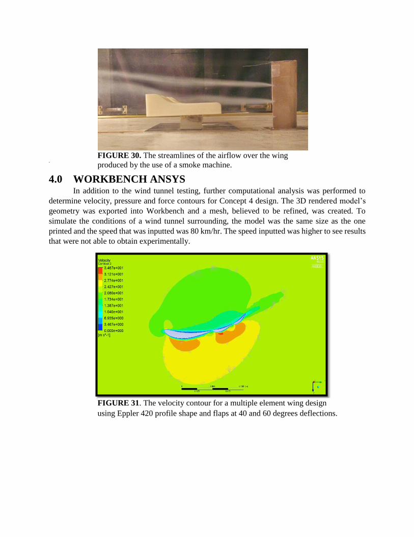
4.0 WORKBENCH ANSYS In addition to the wind tunnel testing, further computational analysis was performed to

determine velocity, pressure and force contours for Concept 4 design. The 3D rendered model’s

geometry was exported into Workbench and a mesh, believed to be refined, was created. To

simulate the conditions of a wind tunnel surrounding, the model was the same size as the one

printed and the speed that was inputted was 80 km/hr. The speed inputted was higher to see results

that were not able to obtain experimentally.

FIGURE 30. The streamlines of the airflow over the wing

produced by the use of a smoke machine.

FIGURE 31. The velocity contour for a multiple element wing design

using Eppler 420 profile shape and flaps at 40 and 60 degrees deflections.

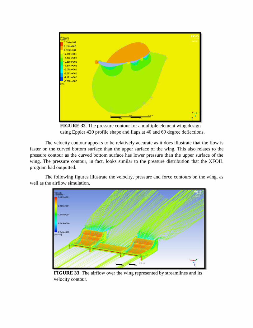
The velocity contour appears to be relatively accurate as it does illustrate that the flow is

faster on the curved bottom surface than the upper surface of the wing. This also relates to the

pressure contour as the curved bottom surface has lower pressure than the upper surface of the

wing. The pressure contour, in fact, looks similar to the pressure distribution that the XFOIL

program had outputted.

The following figures illustrate the velocity, pressure and force contours on the wing, as

well as the airflow simulation.

FIGURE 32. The pressure contour for a multiple element wing design

using Eppler 420 profile shape and flaps at 40 and 60 degree deflections.

FIGURE 33. The airflow over the wing represented by streamlines and its

velocity contour.

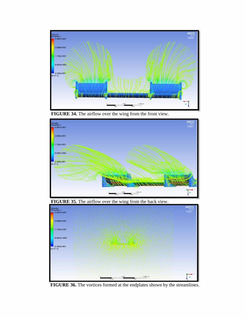
FIGURE 35. The airflow over the wing from the back view.

FIGURE 34. The airflow over the wing from the front view.

FIGURE 36. The vortices formed at the endplates shown by the streamlines.

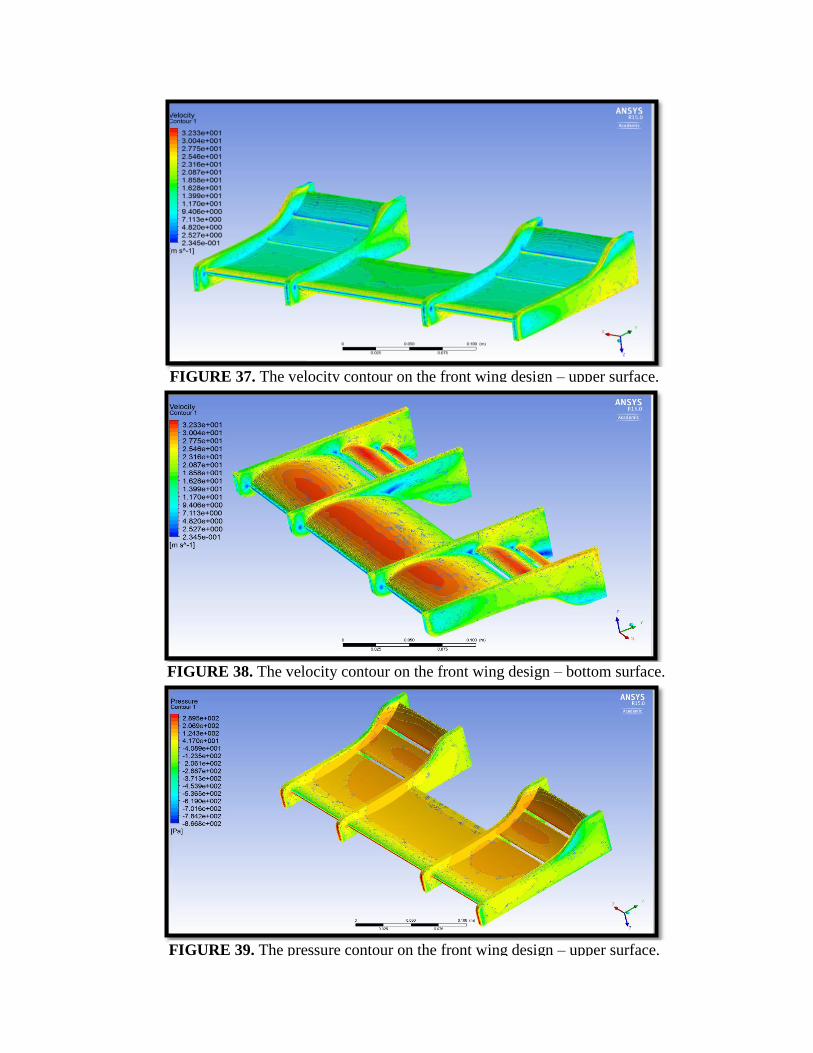
FIGURE 37. The velocity contour on the front wing design – upper surface.

FIGURE 38. The velocity contour on the front wing design – bottom surface.

FIGURE 39. The pressure contour on the front wing design – upper surface.

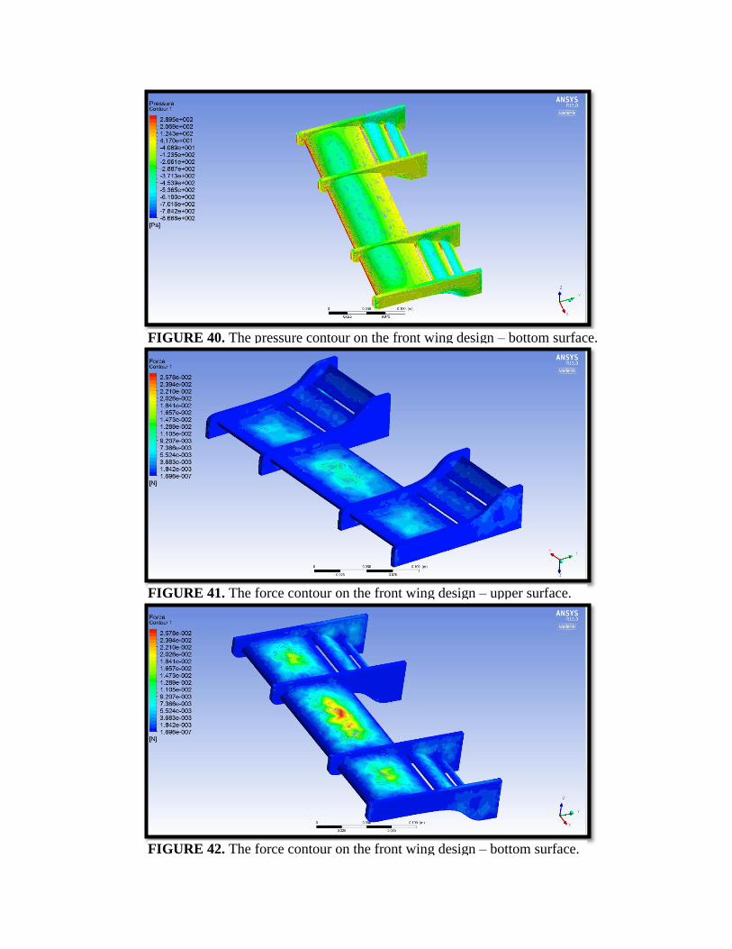
FIGURE 40. The pressure contour on the front wing design – bottom surface.

FIGURE 41. The force contour on the front wing design – upper surface.

FIGURE 42. The force contour on the front wing design – bottom surface.

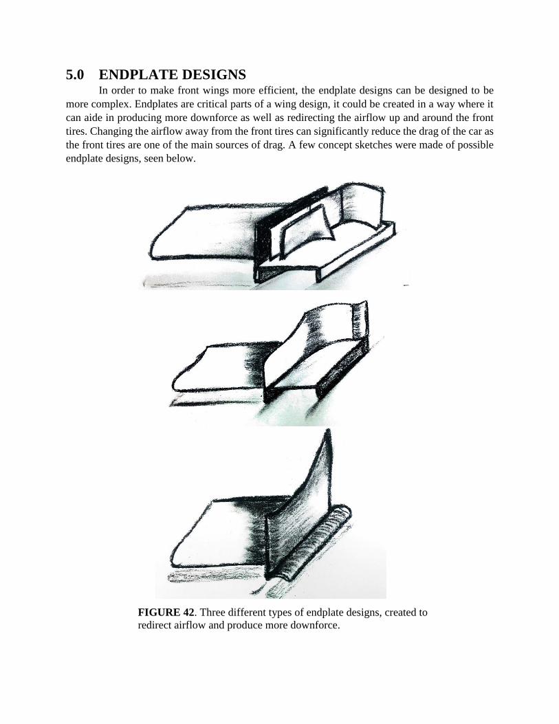
5.0 ENDPLATE DESIGNS In order to make front wings more efficient, the endplate designs can be designed to be

more complex. Endplates are critical parts of a wing design, it could be created in a way where it

can aide in producing more downforce as well as redirecting the airflow up and around the front

tires. Changing the airflow away from the front tires can significantly reduce the drag of the car as

the front tires are one of the main sources of drag. A few concept sketches were made of possible

endplate designs, seen below.

FIGURE 42. Three different types of endplate designs, created to

redirect airflow and produce more downforce.

6.0 CONCLUSION According to the results obtained from the wind tunnel testing, the Concept 4 wing

produced significantly higher downforce than Concept 1, proving that multiple elements are more

beneficial. The values that the Concept 4 wing produced results in a conclusion that front wings

do have a performance advantage, though it may not be as high as the values obtained from the

testing. One entire engineering product cycle has been completed this year, so for the future

aerodynamics role, it is recommended to build a life size scale front wing. With a life size wing,

the weight and drag effects to the amount of downforce the wing is producing, can be compared

and then firmly concluded if a front wing should be a part of the future FSAE cars

7.0 REFERENCES

[1] Wikipedia, "XFOIL," 1 March 2015. [Online]. Available: http://en.wikipedia.org/wiki/XFOIL

APPENDIX A

-4.5

-4

-3.5

-3

-2.5

-2

-1.5

-1

-0.5

0

0 5 10 15 20 25 30 35 40 45 50

MIC

RO

ST

RA

IN

SPEED [KM/HR]

MICROSTRAIN VS. SPEED

Test Run 2 Test Run 1 Test Run 3 Test Run 4 Test Run 5

FIGURE 44. The single element wing’s (printed model) downforce results – raw data.

FIGURE 45. The single element wing’s (printed model) downforce results – raw data

smoothened.

-4.5

-4

-3.5

-3

-2.5

-2

-1.5

-1

-0.5

0

0 5 10 15 20 25 30 35 40 45 50

MIC

RO

ST

RA

IN

SPEED [KM/HR]

MICROSTRAIN VS. SPEEDTest Run 1 Test Run 2 Test Run 3 Test Run 4 Test Run 5

-22

-20

-18

-16

-14

-12

-10

-8

-6

-4

-2

0

0 5 10 15 20 25 30 35 40 45 50

MIC

RO

ST

RA

IN

SPEED [KM/H]

MICROSTRAIN VS. SPEEDTest Run 1 Test Run 2 Test Run 3 Test Run 4 Test Run 5

-20

-18

-16

-14

-12

-10

-8

-6

-4

-2

0

0 5 10 15 20 25 30 35 40 45 50

MIC

RO

ST

RA

IN

SPEED [KM/H]

MICROSTRAIN VS. SPEEDTest Run 1 Test Run 2 Test Run 3 Test Run 4 Test Run 5

FIGURE 46. The multiple element wing’s (printed model) downforce results – raw data.

FIGURE 47. The multiple element wing’s (printed model) downforce results – raw data

smoothened.