AERMOD – 03/19/2004 1

AERMOD Deposition Algorithms – Science Document (Revised Draft)

This Science Document describes the equations used to implement the dry and wet deposition algorithms contained in the AERMOD model, based on the draft Argonne National Laboratory (ANL) report (Wesely, et al., 2001), with modifications based on peer review. Treatment of wet deposition is revised based on recommendations by peer review panel members (Walcek, et al., 2001).

The dry deposition algorithms are described first, followed by the wet deposition algorithms. Within each type of deposition, the particle mode deposition is described first followed by the algorithms for gaseous deposition. Dry Deposition Algorithms

The dry deposition flux, Fd, is calculated as the product of the concentration, χd, and a deposition velocity, Vd, computed at a reference height, zr:

ddd VF ⋅= χ (1)

where Fd = dry deposition flux (µg/m2/s), χd = concentration (µg/m3), calculated at reference height, zr, Vd = deposition velocity (m/s), zr = deposition reference height (m) = zo+1, and zo = surface roughness length for the application site (m), from the meteorological file. The dry deposition flux is calculated on an hourly basis, and summed to obtain the total flux for the user-specified period. The default output units for dry deposition flux are g/m2. Particle Dry Deposition

The dry deposition velocities of particulate HAPs are simulated with a resistance scheme in which the deposition velocity is determined based on the predominant particle size distribution, as described below:

Method 1: Method 1 is used when a significant fraction (greater than about 10 percent) of the total

particulate mass has a diameter of 10 µm or larger. The particle size distribution must be known reasonably well in order to use Method 1. Equation 1 is applied for each particle size category specified by the user, and the results are summed by the model.

The particle deposition velocity, Vdp, for Method 1 is given as,

AERMOD – 03/19/2004 2

ggpapa

dp VVRRRR

V +++

=1 (2)

where Vdp = deposition velocity for particles (m/s), Ra = aerodynamic resistance (s/m), Rp = quasilaminar sublayer resistance (s/m), and Vg = gravitational settling velocity for particles (m/s).

The aerodynamic resistance, Ra, is calculated as follows: for stable and neutral conditions (L > 0),

( )Rku

zz

zLa

r

o

r=⎛⎝⎜

⎞⎠⎟ +

⎡

⎣⎢

⎤

⎦⎥

1 5

*

ln (3a)

for unstable conditions (L < 0),

( )Rku

zL

zL

zL

zL

a

r o

r o

=

− −⎛

⎝⎜

⎞

⎠⎟ − +⎛

⎝⎜

⎞

⎠⎟

− +⎛

⎝⎜

⎞

⎠⎟ − −⎛

⎝⎜

⎞

⎠⎟

⎡

⎣

⎢⎢⎢⎢⎢

⎤

⎦

⎥⎥⎥⎥⎥

11 16 1 1 16 1

1 16 1 1 16 1*

ln (3b)

where k = von Karman constant (0.4), u* = friction velocity (m/s) from the meteorological file, and L = Monin-Obukhov length scale (m) from the meteorological file.

For Method 1, the quasilaminar sublayer resistance, Rp, is calculated as follows:

RSc w u up St=

+ +− −

110 1 0 242 3 3 2 2( ) ( . / )/ /

* * * (4)

where Sc = Schmidt number (Sc = υ/DB) (dimensionless), υ = kinematic viscosity of air (≈ 0.1505 x 10-4 m2/s, and corrected below), DB = Brownian diffusivity (cm2/s) of the pollutant in air, St = Stokes number [St = (Vg/g)(u*

2/υ)] (dimensionless), g = acceleration due to gravity (9.80616 m/s2), and w* = convective velocity scale (m/s) from the meteorological file.

AERMOD – 03/19/2004 3

The kinematic viscosity of air (υ) used in Equation 4 is corrected based on the hourly ambient air temperature and pressure as follows:

[ ])(0132.01101505.0 00

772.1

0

4 PPPP

TTa −+⎟⎟

⎠

⎞⎜⎜⎝

⎛⎟⎟⎠

⎞⎜⎜⎝

⎛×= −υ (5)

where Ta = ambient air temperature (K) from the meteorological file, T0 = reference air temperature = 273.16 K, P = ambient air pressure (kPa) from the meteorological file, and P0 = reference pressure = 101.3 kPa. The Brownian diffusivity of the pollutant, DB (cm2/s) is computed from the following relationship:

⎥⎥⎦

⎤

⎢⎢⎣

⎡

p

CFaB d

STD 10 x 8.09 = 10- (7)

where dp = particle diameter input by user (µm), and SCF = slip correction factor (dimensionless), which is computed as:

p

xda

CF deaax

Sp

4

)/(212

10)(2

123

−

−++= (9)

where x2, a1, a2, a3 are constants with values of 6.5 x 10-6, 1.257, 0.4, and 0.55 x 10-4, respectively.

The gravitational settling velocity, Vg (m/s), is calculated as follows:

CFpAIR

g Scdg

Vµ

ρρ18

)( 22−

= (8)

where ρ = particle density input by user (g/cm3), ρAIR = air density (≈ 1.2 x 10-3 g/cm3), µ = absolute viscosity of air (≈ 1.81 x 10-4 g/cm/s), and c2 = air units conversion constant (1.0 x 10-8 cm2/µm2).

AERMOD – 03/19/2004 4

Method 2:

Method 2 is used when the particle size distribution is not well known and when a small fraction (less than 10 percent of the mass) is in particles with a diameter of 10 µm or larger. The deposition velocity for Method 2 is given as the weighted average of the deposition velocity for particles in the fine mode (i.e., less than 2.5 µm in diameter) and the deposition velocity for the coarse mode (i.e., greater than 2.5 µm but less than 10 µm in diameter):

V f V f Vdp p dpf p dpc= + −( )1 (10) where Vdp = overall particle deposition velocity (m/s), fp = fraction of particulate substance that is fine mode (smaller than 2.5 µm in diameter), input by the user from Appendix B of ANL report (Wesely, et al., 2001), Vdpf = deposition velocity (m/s) of fine particulate substance, calculated from Equation 2

with Vg set to zero; pa

dpf RRV

+=

1 , and

Vdpc = deposition velocity (m/s) of coarse particulate substance, calculated from Equation 2

with Vg = 0.002 m/s; 002.0002.0

1+

++=

papadpc RRRR

V

For Method 2, the aerodynamic resistance is calculated using Equation 3, and the

quasilaminar sublayer resistance, Rp, is calculated with parameterizations based on observations of sulfate dry deposition. For stable and neutral conditions (L > 0),

Rup =

500

* (11a)

for unstable conditions (L < 0),

Ru

L

p =−

⎛⎝⎜

⎞⎠⎟

500

1300

*

(11b)

Gaseous Dry Deposition

For dry deposition of gases, the deposition velocity is given as,

VR R Rdg

a b c=

+ +1

(12)

where

AERMOD – 03/19/2004 5

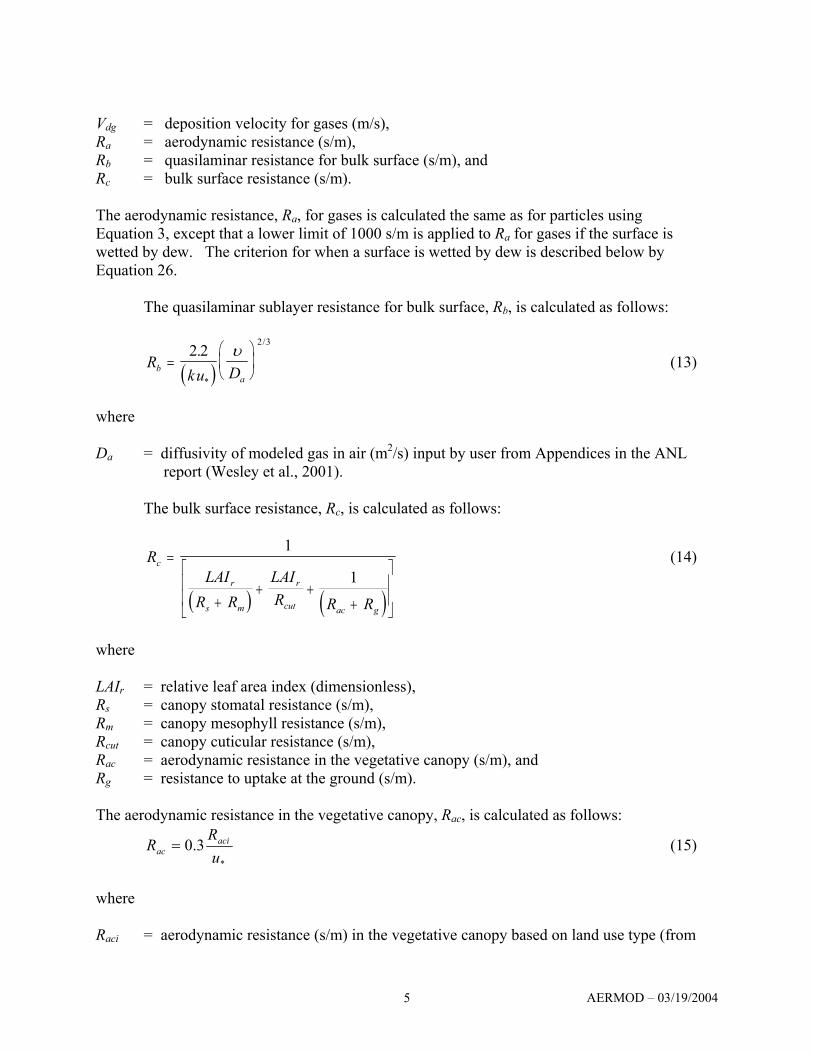
Vdg = deposition velocity for gases (m/s), Ra = aerodynamic resistance (s/m), Rb = quasilaminar resistance for bulk surface (s/m), and Rc = bulk surface resistance (s/m). The aerodynamic resistance, Ra, for gases is calculated the same as for particles using Equation 3, except that a lower limit of 1000 s/m is applied to Ra for gases if the surface is wetted by dew. The criterion for when a surface is wetted by dew is described below by Equation 26.

The quasilaminar sublayer resistance for bulk surface, Rb, is calculated as follows:

( )Rku Db

a=

⎛⎝⎜

⎞⎠⎟

2 22 3

.

*

/υ

(13)

where Da = diffusivity of modeled gas in air (m2/s) input by user from Appendices in the ANL

report (Wesley et al., 2001).

The bulk surface resistance, Rc, is calculated as follows:

( ) ( )

RLAI

R RLAIR R R

c

r

s m

r

cut ac g

=

++ +

+

⎡

⎣

⎢⎢

⎤

⎦

⎥⎥

1

1 (14)

where LAIr = relative leaf area index (dimensionless), Rs = canopy stomatal resistance (s/m), Rm = canopy mesophyll resistance (s/m), Rcut = canopy cuticular resistance (s/m), Rac = aerodynamic resistance in the vegetative canopy (s/m), and Rg = resistance to uptake at the ground (s/m). The aerodynamic resistance in the vegetative canopy, Rac, is calculated as follows:

*

3.0u

RR aci

ac = (15)

where Raci = aerodynamic resistance (s/m) in the vegetative canopy based on land use type (from

AERMOD – 03/19/2004 6

Table 1) and obtained from Table 2. The relative leaf area index is calculated as follows, based on land use type (from Table 1) and season (defined below):

LAI Fr = for land use types 4 and 6 (forests), and (16a)

LAI Fr = 0 5. for all other land use types. (16b) F depends on the user specified seasonal category, based on the following general characteristics:

1. Midsummer with lush vegetation 2. Autumn with unharvested cropland 3. Late autumn after frost and harvest, or winter with no snow 4. Winter with snow on the ground 5. Transitional spring with partial green coverage or short annuals

F = 1 for categories 1, 3, and 4

F is set to the user input value for categories 2 and 5, or to the default values of: F = 0.5 for category 2, and F = 0.25 for category 5.

The canopy stomatal resistance, Rs, is calculated as follows:

( )R RDD f f f fs i

v

a=

⎛⎝⎜

⎞⎠⎟

1

1 2 3 4

(17)

where Ri = minimum stomatal resistance (s/m) from Table 2, Dv = diffusivity of water vapor in air (0.219 x 10-4 m2/s), f1 = multiplicative scaling factors for solar irradiance (dimensionless), f2 = multiplicative scaling factor for soil moisture (dimensionless), f3 = multiplicative scaling factor for humidity (dimensionless), and f4 = multiplicative scaling factor for temperature (dimensionless).

The multiplicative scaling factor for solar irradiance, f1, is calculated as follows: ( )( )f

G G

G Gr

r1

0 01

1=

+

+

/ .

/ (18)

where

AERMOD – 03/19/2004 7

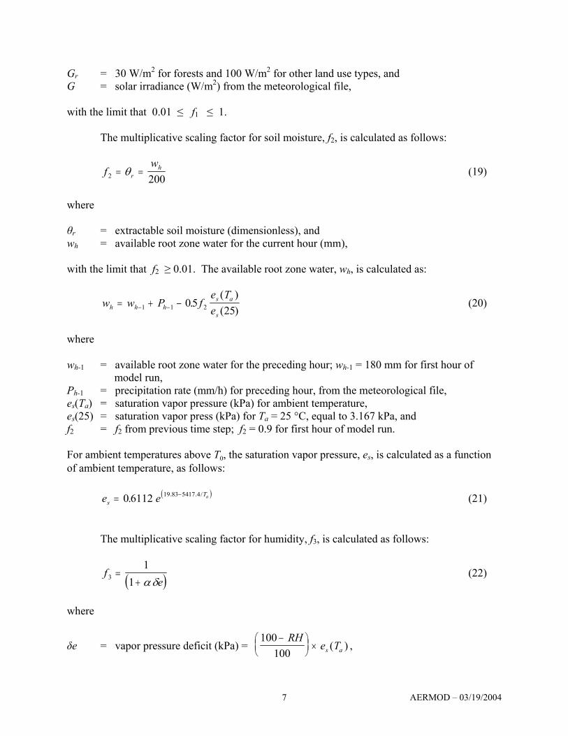
Gr = 30 W/m2 for forests and 100 W/m2 for other land use types, and G = solar irradiance (W/m2) from the meteorological file, with the limit that 0.01 ≤ f1 ≤ 1.

The multiplicative scaling factor for soil moisture, f2, is calculated as follows:

fw

rh

2 200= =θ (19)

where θr = extractable soil moisture (dimensionless), and wh = available root zone water for the current hour (mm), with the limit that f2 ≥ 0.01. The available root zone water, wh, is calculated as:

w w P fe Teh h h

s a

s= + −− −1 1 205

25.

( )( )

(20)

where wh-1 = available root zone water for the preceding hour; wh-1 = 180 mm for first hour of

model run, Ph-1 = precipitation rate (mm/h) for preceding hour, from the meteorological file, es(Ta) = saturation vapor pressure (kPa) for ambient temperature, es(25) = saturation vapor press (kPa) for Ta = 25 °C, equal to 3.167 kPa, and f2 = f2 from previous time step; f2 = 0.9 for first hour of model run. For ambient temperatures above T0, the saturation vapor pressure, es, is calculated as a function of ambient temperature, as follows:

( )e esTa= −0 6112 19 83 5417 4. . . / (21)

The multiplicative scaling factor for humidity, f3, is calculated as follows:

( )fe3

11

=+ αδ

(22)

where

δe = vapor pressure deficit (kPa) = 100

100−⎛

⎝⎜⎞⎠⎟ ×

RHe Ts a( ) ,

AERMOD – 03/19/2004 8

RH = relative humidity (percent) from the meteorological file, and α = coefficient = 0.1 kPa-1, with the limit that f3 ≥ 0.01.

The multiplicative scaling factor for temperature, f4, is calculated as follows:

f Ta421 0 0016 298 0= − −. ( . ) (23)

with the limit that f4 ≥ 0.01 .

The bulk canopy leaf mesophyll resistance, Rm (s/m) in Equation 14, is calculated as follows:

R

Hf

m

o

=+

⎛⎝⎜

⎞⎠⎟

10 034

100. (24)

where H = Henry’s Law Constant input by user (Pa-m3/mol), fo = reactivity factor (dimensionless), and is equal to: 1.0 for ozone, titanium tetrachloride, and divalent mercury, 0.1 for nitrogen oxide, and 0 for other substances.

The canopy cuticular resistance, Rcut, is calculated as follows:

( )

R

H Rf f H

R R

cut

cS

o o

cO cl

=

++

+⎡

⎣⎢⎢

⎤

⎦⎥⎥

−

1

10 13 2( / ) (25)

where RcS = resistance to SO2 uptake by cuticle (s/m), from Table 2 if dry, and is equal to

50 s/m if canopy is wetted by rain or dew, RcO = resistance to O3 uptake by cuticle (s/m), from Table 2 if dry, and is equal to

0.75 times RcO from Table 2 if canopy is wetted by rain or dew, and Rcl = bulk canopy cuticular resistance (s/m) by lipid solubility, defined below.

The surface is assumed to be wetted by rain if precipitation occurs within the previous two hours. However, the adjustments to RcS and RcO for wetted surface are not applied if the seasonal category is 4 (winter with snow), the precipitation code for the current hour indicates frozen precipitation, and the ambient temperature is below freezing.

AERMOD – 03/19/2004 9

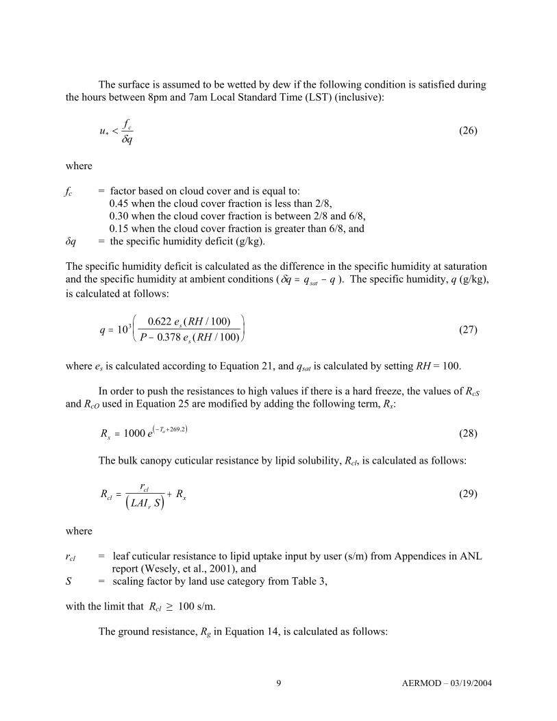
The surface is assumed to be wetted by dew if the following condition is satisfied during

the hours between 8pm and 7am Local Standard Time (LST) (inclusive):

qf

u c

δ<* (26)

where fc = factor based on cloud cover and is equal to:

0.45 when the cloud cover fraction is less than 2/8, 0.30 when the cloud cover fraction is between 2/8 and 6/8, 0.15 when the cloud cover fraction is greater than 6/8, and

δq = the specific humidity deficit (g/kg). The specific humidity deficit is calculated as the difference in the specific humidity at saturation and the specific humidity at ambient conditions (δq q qsat= − ). The specific humidity, q (g/kg), is calculated at follows:

qe RH

P e RHs

s=

−⎛⎝⎜

⎞⎠⎟10

0 622 1000 378 100

3 . ( / ). ( / )

(27)

where es is calculated according to Equation 21, and qsat is calculated by setting RH = 100.

In order to push the resistances to high values if there is a hard freeze, the values of RcS and RcO used in Equation 25 are modified by adding the following term, Rx:

( )R exTa= − +1000 269 2. (28)

The bulk canopy cuticular resistance by lipid solubility, Rcl, is calculated as follows:

( )Rr

LAI SRcl

cl

rx= + (29)

where rcl = leaf cuticular resistance to lipid uptake input by user (s/m) from Appendices in ANL report (Wesely, et al., 2001), and S = scaling factor by land use category from Table 3, with the limit that Rcl ≥ 100 s/m.

The ground resistance, Rg in Equation 14, is calculated as follows:

AERMOD – 03/19/2004 10

( )

R

H R

f f HR

g

gS

o o

gO

=

++⎡

⎣

⎢⎢

⎤

⎦

⎥⎥

−

1

10 013 2( . / ) (30)

where RgS = resistance to SO2 uptake by ground (s/m), from Table 2 if dry, and is equal to

50 s/m if canopy is wetted by rain or dew, and RgO = resistance to O3 uptake by ground (s/m), from Table 2. As with the cuticular resistances in Equation 25, in order to push the ground resistances to a high value if there is a hard freeze, the values of RgS and RgO used in Equation 30 are modified by adding the term Rx, calculated from Equation 28. In addition, the adjustment to RgS for wetted surface is not applied if the seasonal category is 4 (winter with snow), the precipitation code for the current hour indicates frozen precipitation, and the ambient temperature is below freezing. Wet Deposition Algorithms Particle Wet Deposition Flux

The wet deposition flux for particulate substances, Fwp, is calculated from the particle-phase washout coefficient as follows:

rWF ppwp ρ310−= (31)

where Fwp = flux of particulate matter by wet deposition (µg/m2/hr), ρp = column average concentration of particulate in air (µg/m3), Wp = particle washout coefficient (dimensionless), and r = water or water equivalent precipitation rate (mm/hr), from the meteorological file. The wet deposition flux is calculated on an hourly basis, and summed to obtain the total flux for the user-specified period. The default output units for wet deposition flux are g/m2. The constant of 10-3 is a conversion factor to convert the precipitation rate units from mm/hr to m/hr.

The column average concentration, ρp, is calculated by integrating the vertical term for the Gaussian plume equation for each particle size category, Vj, over all heights (z), such that

πσ

20

=⎟⎟⎠

⎞⎜⎜⎝

⎛∫

pz

z

j dzV

(32)

where

AERMOD – 03/19/2004 11

Vj = Gaussian vertical term for particle size category j, σz = vertical dispersion coefficient (m), and zp = height of the top of plume or mixing height, whichever is greater (m). The height of the top of the plume used to define zp is calculated as the plume centerline height plus 2.15 times σz, evaluated at a downwind distance of 20 kilometers. The integrated vertical term from Equation 32 is then multiplied by the other terms in the Gaussian plume equation that do not vary with height, including the emission rate and lateral dispersion term, to obtain the vertically integrated concentration. Dividing by the height of the vertical column, zp, then provides the column average concentration.

The particle washout coefficient, Wp, is calculated as follows:

m

pp D

EzW

23

= (33)

where, E = collision efficiency (dimensionless), and Dm = mean diameter of raindrop (m) = r0.232/905.5 with r in mm/hr. It is assumed that the washout coefficient, Wp, and therefore the wet deposition flux, Fwp, is the same for frozen precipitation as for liquid precipitation. The collision efficiency, E, is calculated as follows, based on Slinn (1984) and Seinfeld and Pandis (1998):

[ ] ( )2/3

*

*2/12/12/12/13/12/1

3221416.04.014

⎟⎟⎟⎟

⎠

⎞

⎜⎜⎜⎜

⎝

⎛

+−

−⎟⎟⎠

⎞⎜⎜⎝

⎛+⎥

⎦

⎤⎢⎣

⎡+++++=

SSt

SStRScRScRScR

E we

wee

e ρρφ

µµφ (34)

where, Re = Reynolds number of raindrop ( υ/fallaV ) (dimensionless), Vfall = precipitation fall speed (m/s) = 3.75 r0.111, with r in mm/hr, N = ratio of particle diameter to raindrop diameter = mp Dd / , µw = viscosity of water (≈ 1.0 x 10-2 g/cm/s), ρw = density of water = 106 g/m3, St = Stokes number of collected particle [St = (Vg/g)(Vfall-Vg)/a)] (dimensionless), and S* = critical Stokes number (dimensionless), calculated as:

( )( )e

e

R

RS

++

++=

1ln1

1ln1212.1

* (35)

AERMOD – 03/19/2004 12

Gaseous Wet Deposition Flux The wet deposition flux for gases, Fwg, is calculated as follows:

rMCF wlwg610= (36)

where Fwg = flux of gaseous pollutants by wet deposition (µg/m2/hr), Cl = concentration of pollutant in the liquid phase (moles/liter), and Mw = molecular weight of pollutant (grams/mole). The wet deposition flux is calculated on an hourly basis, and summed to obtain the total flux for the user-specified period. The default output units for wet deposition flux are g/m2. The constant of 106 is a combined conversion factor to convert the precipitation rate units from mm/hr to m/hr, to convert volume from liters to m3, and to convert from µg to grams. As with particle wet deposition, the wet deposition flux for gases is assumed to be the same for frozen and liquid precipitation.

The concentration of pollutant in liquid phase, Cl, is calculated based on the saturated concentration, Clsat, and the fraction of saturation, fsat:

lsatsatl CfC = (37)

where fsat = fraction of saturation (dimensionless), and Clsat = concentration of pollutant in liquid phase at saturation (moles/liter). The pollutant concentration in liquid phase at concentration, Clsat, is calculated as follows:

⎥⎦

⎤⎢⎣

⎡+

=

HTRL

MH

TRC

w

aww

aglsat

ρ

ρ

1109

(38)

where ρg = column average concentration of gaseous pollutant in air (µg/m3), R = universal gas constant = 8.3145 Pa-m3/mole-K, Lw = liquid water content of falling rain (g/m3) = r0.889/13.28, with r in mm/hr.

AERMOD – 03/19/2004 13

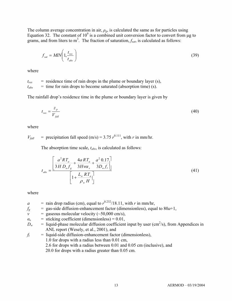
The column average concentration in air, ρg, is calculated the same as for particles using Equation 32. The constant of 109 is a combined unit conversion factor to convert from µg to grams, and from liters to m3. The fraction of saturation, fsat, is calculated as follows:

⎟⎟⎠

⎞⎜⎜⎝

⎛=

abs

ressat t

tMINf ,1 (39)

where tres = residence time of rain drops in the plume or boundary layer (s), tabs = time for rain drops to become saturated (absorption time) (s). The rainfall drop’s residence time in the plume or boundary layer is given by

fall

pres V

zt = (40)

where Vfall = precipitation fall speed (m/s) = 3.75 r0.111, with r in mm/hr.

The absorption time scale, tabs, is calculated as follows:

⎥⎦

⎤⎢⎣

⎡+

⎥⎥⎦

⎤

⎢⎢⎣

⎡++

=

HTRL

fDa

HTRa

fDHTRa

t

w

aw

lws

a

ga

a

abs

ρ

να

1

317.0

34

3

22

(41)

where a = rain drop radius (cm), equal to r0.232/18.11, with r in mm/hr, fg = gas-side diffusion-enhancement factor (dimensionless), equal to 80a+1, ν = gaseous molecular velocity (~50,000 cm/s), αs = sticking coefficient (dimensionless) = 0.01, Dw = liquid-phase molecular diffusion coefficient input by user (cm2/s), from Appendices in ANL report (Wesely, et al., 2001), and fl = liquid-side diffusion-enhancement factor (dimensionless), 1.0 for drops with a radius less than 0.01 cm, 2.6 for drops with a radius between 0.01 and 0.05 cm (inclusive), and 20.0 for drops with a radius greater than 0.05 cm.

AERMOD – 03/19/2004 14

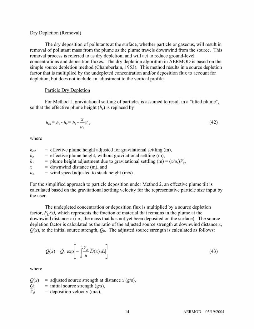
Dry Depletion (Removal) The dry deposition of pollutants at the surface, whether particle or gaseous, will result in removal of pollutant mass from the plume as the plume travels downwind from the source. This removal process is referred to as dry depletion, and will act to reduce ground-level concentrations and deposition fluxes. The dry depletion algorithm in AERMOD is based on the simple source depletion method (Chamberlain, 1953). This method results in a source depletion factor that is multiplied by the undepleted concentration and/or deposition flux to account for depletion, but does not include an adjustment to the vertical profile. Particle Dry Depletion For Method 1, gravitational settling of particles is assumed to result in a "tilted plume", so that the effective plume height (he) is replaced by

Vux - h = h - h = h g

seveed (42)

where hed = effective plume height adjusted for gravitational settling (m), he = effective plume height, without gravitational settling (m), hv = plume height adjustment due to gravitational settling (m) = (x/us)Vg, x = downwind distance (m), and us = wind speed adjusted to stack height (m/s). For the simplified approach to particle deposition under Method 2, an effective plume tilt is calculated based on the gravitational settling velocity for the representative particle size input by the user. The undepleted concentration or deposition flux is multiplied by a source depletion factor, FQ(x), which represents the fraction of material that remains in the plume at the downwind distance x (i.e., the mass that has not yet been deposited on the surface). The source depletion factor is calculated as the ratio of the adjusted source strength at downwind distance x, Q(x), to the initial source strength, Q0. The adjusted source strength is calculated as follows:

⎥⎦

⎤⎢⎣

⎡−= ∫

xd dxxD

uV

QxQ0

0 )(exp)( (43)

where Q(x) = adjusted source strength at distance x (g/s), Q0 = initial source strength (g/s), Vd = deposition velocity (m/s),

AERMOD – 03/19/2004 15

u = transport wind speed (m/s), )(xD = crosswind integrated diffusion function, QuD /χ= (m-1), and

χ = crosswind integrated concentration (g/m2) Gaseous Dry Depletion The dry depletion (removal) of gaseous plumes is calculated using the same approach as described above for dry depletion of particulate plumes, except that there is no vertical tilt to the plume centerline height, i.e., the gravitational settling velocity, Vg, is set to 0.0 in Equation 42 and hed = he. Wet Depletion (Removal) The wet deposition or washout of pollutant by precipitation, whether particle or gaseous, will remove pollutant mass as the plume travels downwind from the source. This removal process is referred to as wet depletion, and will act to reduce ground-level concentrations and deposition fluxes. Since the washout of pollutants due to precipitation occurs through the full vertical extent of the plume, the wet depletion algorithm in AERMOD is based on a source depletion approach that calculates the fraction of plume material that has been removed from the plume, and multiplies the source depletion factor times the undepleted concentration and/or deposition flux.

The wet depletion factor, i.e., the ratio of the source strength modified by depletion at the receptor location (Q(x)) to the original unmodified source strength (Q0), is calculated as follows:

teQ

xQ Λ−=0

)( (44)

where Q0 = unmodified source strength (g/s), Q(x) = source strength modified for wet depletion at downwind distance x (g/s), Λ = equivalent scavenging ratio (s-1), and t = plume travel time from source to receptor (s) = x/u . The wet depletion factor calculated from Equation 43 is then multiplied by the undepleted concentration and/or deposition flux to account for removal of plume mass due to wet depletion. Particle Wet Depletion

For particle wet depletion, the equivalent scavenging ratio, Λ, in Equation 43 is calculated based on the wet time scale, i.e., the time scale for removal of pollutant from the plume by precipitation. The wet time scale is given by the mass of pollutant in the column of air divided by the flux of pollutant out of the column:

AERMOD – 03/19/2004 16

wp

pp

Fz

leWetTimeScaρ

=Λ= −1 (45)

Substituting for Fwp from Equation 31 into Equation 45 and using Equation 33 yields the following equation for the equivalent scavenging ratio, Λ (s-1):

60

106.323

×=Λ

mDrE

(46)

where the constant 3.6 × 106 converts units from meters to mm and from hours to seconds. Gaseous Wet Depletion The wet depletion factor for gaseous pollutants is calculated similar to the wet depletion factor for particles using Equation 43, and with an equivalent scavenging ratio defined based on the wet time scale, i.e.,

wg

pg

Fz

leWetTimeScaρ

=Λ= −1 (47)

As with particle wet depletion, substituting for Fwg from Equation 36 into Equation 47 with Equations 37 and 38 yields the following equation for the equivalent scavenging ratio, Λ (s-1):

⎥⎦

⎤⎢⎣

⎡+×

=Λ

HTRL

Hz

rTRf

w

ap

asat

ρ1106.3 6

(48)

where the constant 3.6 × 106 converts units from meters to mm and from hours to seconds.

AERMOD – 03/19/2004 17

Table 1. Land Use Types

__________________________________________ No. Land Use Type

__________________________________________

1 Urban land, no vegetation 2 Agricultural land 3 Rangeland 4 Forest 5 Suburban areas, grassy 6 Suburban areas, forested 7 Bodies of water 8 Barren land, mostly desert 9 Non-forested wetlands

__________________________________________

AERMOD – 03/19/2004 18

Table 2. Values of surface resistances (s/m) by land use type and seasonal category

Land Use Type Resistance 1 2 3 4 5 6 7 8 9Season #1: Midsummer with lush vegetation Ri 1.e07 60. 120. 100. 200. 150. 1.e07 1.e07 80.RcS 1.e07 2000. 2000. 2000. 2000. 2000. 1.e07 1.e07 2500.RcO 1.e07 1000. 1000. 1000. 2000. 2000. 1.e07 1.e07 1000.Raci 100. 200. 100. 2000. 100. 1500. 0. 0. 300.RgS 400. 150. 350. 300. 500. 450. 0. 1000. 0.RgO 300. 150. 200. 200. 300. 300. 2000. 400. 1000.Season #2: Autumn with unharvested cropland Ri 1.e07 1.e07 1.e07 350. 1.e07 700. 1.e07 1.e07 1.e07RcS 1.e07 6500. 6500. 3000. 2000. 2000. 1.e07 1.e07 6500.RcO 1.e07 400. 300. 500. 600. 1000. 1.e07 1.e07 300.Raci 100. 150. 100. 1700. 100. 1200. 0. 0. 200.RgS 400. 200. 350. 300. 500. 450. 0. 1000. 0.RgO 300. 150. 200. 200. 300. 300. 2000. 400. 800.Season #3: Late autumn after frost and harvest, or winter with no snow Ri 1.e07 1.e07 1.e07 500. 1.e07 1000. 1.e07 1.e07 1.e07RcS 1.e07 1.e07 9000. 6000. 2000. 2000. 1.e07 1.e07 9000.RcO 1.e07 1.e07 400. 600. 800. 1600. 1.e07 1.e07 800.Raci 100. 0. 100. 1500. 100. 1000. 0. 0. 100.RgS 400. 150. 350. 300. 500. 450. 0. 0. 1000.RgO 300. 150. 200. 200. 300. 300. 2000. 400. 1000.Season #4: Winter with snow on the ground Ri 1.e07 1.e07 1.e07 800. 1.e07 1600. 1.e07 1.e07 1.e07RcS 1.e07 1.e07 1.e07 400. 1.e07 800. 1.e07 1.e07 9000.RcO 1.e07 2000. 1000. 600. 2000. 1200. 1.e07 1.e07 800.Raci 100. 0. 10. 1500. 100. 1000. 0. 0. 50.RgS 100. 100. 100. 100. 200. 200. 0. 1000. 100.RgO 600. 3500. 3500. 3500. 500. 500. 2000. 400. 3500.Season #5: Transitional spring with partial green coverage or short annuals Ri 1.e07 100. 120. 100. 200. 150. 1.e07 1.e07 80.RcS 1.e07 2000. 2000. 1500. 2000. 2000. 1.e07 1.e07 2000.RcO 1.e07 1000. 250. 350. 500. 700. 1.e07 1.e07 300.Raci 100. 50. 80. 1500. 100. 1000. 0. 0. 200.RgS 500. 150. 350. 300. 500. 450. 0. 1000. 0.RgO 300. 150. 200. 200. 300. 300. 2000. 400. 1000.

AERMOD – 03/19/2004 19

Table 3. Values of factor S for scaling rcl

__________________________________________

Land Use Cat. Scaling Factor __________________________________________

1 1.0×10-5 2 6 3 5 4 7 5 3 6 4 7 1.0×10-5 8 1.0×10-5 9 3

__________________________________________ References Chamberlain, A. C., 1953: Aspects of travel and deposition of aerosol and vapor clouds. Atomic Energy Research Establishment, HP/R 1261. Seinfeld, J. H. and S. N. Pandis, 1998: Atmospheric Chemistry and Physics, John Wiley & Sons, Inc., New York, NY. Slinn, W. G. N., 1984: Precipitation Scavenging, in Atmospheric Science and Power Production, D. Randerson (ed.). DOE/TIC-27601. U. S. Department of Energy, Washington, DC. Walcek, C., G. Stensland, L. Zhang, H. Huang, J. Hales, C. Sweet, W. Massman, A. Williams, J, Dicke, 2001: Scientific Peer-Review of the Report “Deposition Parameterization for the Industrial Source Complex (ISC3) Model.” The KEVRIC Company, Durham, North Carolina. Wesely, M. L, P. V. Doskey, and J.D. Shannon, 2001: Deposition Parameterizations for the Industrial Source Complex (ISC3) Model. Draft ANL report ANL/ER/TM-nn, DOE/xx-nnnn, Argonne National Laboratory, Argonne, Illinois 60439.

AERMOD – 03/19/2004 20

List of Symbols a = rain drop radius (cm) Cl = concentration of pollutant in the liquid phase (moles/liter) Clsat = concentration of pollutant in liquid phase at saturation (moles/liter) c2 = air units conversion constant (1.0 x 10-8 cm2/µm2) Da = diffusivity of modeled gas in air (m2/s) DB = Brownian diffusivity (cm2/s) of the pollutant in air Dm = mean diameter of raindrop (m) Dv = diffusivity of water vapor in air (0.219 x 10-4 m2/s) Dw = liquid-phase molecular diffusion coefficient input by user (cm2/s) dp = particle diameter input by user (µm) E = collision efficiency (dimensionless) es(25) = saturation vapor press (kPa) for Ta = 25 °C, equal to 3.167 kPa es(Ta) = saturation vapor pressure (kPa) for ambient temperature Fd = dry deposition flux (µg/m2/s) Fwg = flux of gaseous pollutants by wet deposition (µg/m2/hr) Fwp = flux of particulate matter by wet deposition (µg/m2/hr) fo = reactivity factor (dimensionless) f1 = multiplicative scaling factors for solar irradiance (dimensionless) f2 = multiplicative scaling factor for soil moisture (dimensionless) f3 = multiplicative scaling factor for humidity (dimensionless) f4 = multiplicative scaling factor for temperature (dimensionless) fc = factor based on cloud cover for dew test (dimensionless) fg = gas-side diffusion-enhancement factor (dimensionless) fl = liquid-side diffusion-enhancement factor (dimensionless) fp = fraction of particulate substance that is fine mode, smaller than 2.5 µm (dimensionless) fsat = fraction of saturation (dimensionless) G = solar irradiance (W/m2) Gr = reference solar irradiance = 30 W/m2 for forests and 100 W/m2 for other land use types g = acceleration due to gravity (9.80616 m/s2) H = Henry’s Law Constant input by user (Pa-m3/mol) he = effective plume height (m) hed = effective plume height, adjusted for gravitational settling (m) hv = plume height adjustment due to gravitational settling (m) k = von Karman constant (0.4) L = Monin-Obukhov length scale (m) Lw = liquid water content of falling rain (g/m3) LAIr = relative leaf area index (dimensionless) Mw = molecular weight of pollutant (grams/mole) P = ambient air pressure (kPa) P0 = reference pressure = 101.3 kPa Ph-1 = precipitation rate (mm/h) for preceding hour Q0 = unmodified source strength (g/s) Q(x) = source strength modified for wet depletion at downwind distance x (g/s) R = universal gas constant = 8.3145 Pa-m3/mole-K

AERMOD – 03/19/2004 21

Ra = aerodynamic resistance (s/m) Rac = aerodynamic resistance in the vegetative canopy (s/m) Raci = aerodynamic resistance (s/m) in the vegetative canopy Rb = quasilaminar resistance for bulk surface (s/m) Rc = bulk surface resistance (s/m) Rcl = bulk canopy cuticular resistance (s/m) by lipid solubility RcO = resistance to O3 uptake by cuticle (s/m) RcS = resistance to SO2 uptake by cuticle (s/m) Rcut = canopy cuticular resistance (s/m) Re = Reynolds number of raindrop (dimensionless) Rg = resistance to uptake at the ground (s/m) RgO = resistance to O3 uptake by ground (s/m) RgS = resistance to SO2 uptake by ground (s/m) Ri = minimum stomatal resistance (s/m) Rm = canopy mesophyll resistance (s/m) Rp = quasilaminar sublayer resistance (s/m) Rs = canopy stomatal resistance (s/m) RH = relative humidity (percent) r = water or water equivalent precipitation rate (mm/hr) rcl = leaf cuticular resistance to lipid uptake input by user (s/m) S = scaling factor by land use category Sc = Schmidt number (Sc = υ/DB) (dimensionless) SCF = slip correction factor (dimensionless) St = Stokes number (dimensionless) S* = critical Stokes number (dimensionless) T0 = reference air temperature = 273.16 K Ta = ambient air temperature (K) t = plume travel time from source to receptor (s) tabs = time for rain drops to become saturated (absorption time) (s) tres = residence time of rain drops in the plume or boundary layer (s) u = transport wind speed (m/s) us = wind speed adjusted to stack height (m/s) u* = friction velocity (m/s) Vd = deposition velocity (m/s) Vdg = deposition velocity for gases (m/s) Vdp = deposition velocity for particles (m/s) Vdpf = deposition velocity (m/s) of fine particulate substance Vdpc = deposition velocity (m/s) of coarse particulate substance Vfall = precipitation fall speed (m/s) Vg = gravitational settling velocity for particles (m/s) Vj = vertical term for particle size category j Wp = particle washout coefficient (dimensionless) wh = available root zone water for the current hour (mm) wh-1 = available root zone water for the preceding hour (mm) w* = convective velocity scale (m/s) x = downwind distance (m)

AERMOD – 03/19/2004 22

zi = mixing height (m) zo = surface roughness length for the application site (m) zp = height of the top of plume or mixing height, whichever is greater (m) zr = deposition reference height (m) = zo+1 α = coefficient = 0.1 kPa-1 αs = sticking coefficient (dimensionless) = 0.01 δe = vapor pressure deficit (kPa) δq = the specific humidity deficit (g/kg) θr = extractable soil moisture (dimensionless) Λ = equivalent scavenging ratio (s-1) µ = absolute viscosity of air (≈ 1.81 x 10-4 g/cm/s) µw = viscosity of water (≈ 1.0 x 10-2 g/cm/s) ν = gaseous molecular velocity (~50,000 cm/s) N = ratio of particle diameter to raindrop diameter (dimensionless) ρ = particle density input by user (g/cm3) ρg = column average concentration of gaseous pollutant in air (µg/m3) ρp = column average concentration of particulate in air (µg/m3) ρAIR = air density (≈ 1.2 x 10-3 g/cm3) ρw = density of water = 106 g/m3 σz = vertical dispersion coefficient (m) υ = kinematic viscosity of air (≈ 0.1505 x 10-4 m2/s) χd = concentration (µg/m3), calculated at reference height, zr