ADVISOR 2.1: A User-FriendlyAdvanced PowertrainSimulation Using a CombinedBackward/Forward Approach

August 1999 • NREL/JA-540-26839

K.B. Wipke, M.R. Cuddy, and S.D. Burch

Preprint prepared for IEEE Transactions onVehicular Technology: Special Issues onHybrid and Electric Vehicles

National Renewable Energy Laboratory1617 Cole BoulevardGolden, Colorado 80401-3393

NREL is a U.S. Department of Energy LaboratoryOperated by Midwest Research Institute •••• Battelle •••• Bechtel

Contract No. DE-AC36-98-GO10337

NOTICE

This report was prepared as an account of work sponsored by an agency of the United Statesgovernment. Neither the United States government nor any agency thereof, nor any of their employees,makes any warranty, express or implied, or assumes any legal liability or responsibility for the accuracy,completeness, or usefulness of any information, apparatus, product, or process disclosed, or representsthat its use would not infringe privately owned rights. Reference herein to any specific commercialproduct, process, or service by trade name, trademark, manufacturer, or otherwise does not necessarilyconstitute or imply its endorsement, recommendation, or favoring by the United States government or anyagency thereof. The views and opinions of authors expressed herein do not necessarily state or reflectthose of the United States government or any agency thereof.

Available to DOE and DOE contractors from:Office of Scientific and Technical Information (OSTI)P.O. Box 62Oak Ridge, TN 37831

Prices available by calling 423-576-8401

Available to the public from:National Technical Information Service (NTIS)U.S. Department of Commerce5285 Port Royal RoadSpringfield, VA 22161703-605-6000 or 800-553-6847orDOE Information Bridgehttp://www.doe.gov/bridge/home.html

Printed on paper containing at least 50% wastepaper, including 20% postconsumer waste

Abstract--ADVISOR 2.1 is the latest version of the NationalRenewable Energy Laboratory’s advanced vehicle simulator.It was first developed in 1994 to support the U.S. Departmentof Energy hybrid propulsion system program, and is designedto be accurate, fast, flexible, easily sharable, and easy to use.This paper presents the model, focusing on its combination offorward- and backward-facing simulation approaches, andevaluates the model in terms of its design goals. ADVISORpredicts acceleration time to within 0.7% and energy use onthe demanding US06 to within 0.6% for an underpoweredseries hybrid vehicle (0-100 km/h in 20 s). ADVISORsimulates vehicle performance on standard driving cyclesbetween 2.6 and 8.0 times faster than a representativeforward-facing vehicle model. Due in large part toADVISOR’s powerful graphical user interface and Webpresence, over 800 users have downloaded ADVISOR from 45different countries. Many of these users have contributedtheir own component data to the ADVISOR library.

I. INTRODUCTION

ADVISOR was first developed in November 1994. Itsmain purpose was to help manage the U.S. Department ofEnergy’s (DOE) hybrid electric vehicle (HEV) programsubcontracts by facilitating our understanding of thetechnical challenges inherent in the design of high-efficiency HEVs. ADVISOR uses drivetrain componentperformance to estimate fuel economy and emissions ongiven cycles as well as maximum-effort accelerationcapability. It is fundamentally an empirical model.

A. Model design

In accordance with ADVISOR’s mission as an analysis toolto support the U.S. DOE hybrid program, we designedADVISOR to meet certain goals. It needed to be- Accurate, allowing meaningful comparison of different

drivetrain configurations- Fast, allowing high-speed analysis of vehicles and

design space investigations, such as multi-dimensionalparametric studies and optimization

- Flexible, allowing us to evaluate vehicles with variouscontrol strategies and combinations of components

- Publicly available, allowing us to share it with potentialcollaborators and also to foster HEV development andunderstanding among the public

The main author is with the National Renewable EnergyLaboratory, Golden, CO 80401 USA.

- Capable of modeling vehicles of any type:conventional, electric, series hybrid, or parallel hybrid

- Easy to use, even for those without detailed knowledgeof vehicle modeling.

Vehicle simulators existing in 1994 were considered for usebefore ADVISOR was developed [1-3]. Existingsimulators were available to NREL only as executablecode. Lack of access to the source code prevented theimplementation of new, unique control strategies and newvehicle configurations with these tools. Also, existingcodes were not designed to fully simulate parallel HEVs orconventional-drivetrain vehicles.

To best meet our design goals, we chose to develop ahybrid backward/forward-facing vehicle simulator in theMATLAB®/Simulink® environment. MATLAB®/Simulink® was chosen for its nearly self-documentinggraphical programming environment and its wideacceptance by researchers in academia and industry.ADVISOR’s hybrid modeling approach was chosen for itscombination of the qualities of the two approaches: high-speed execution and good prediction of maximum effortaccelerations (and other component-limited conditions).For reference, the two main vehicle simulation approachesare described below, followed by an in-depth discussion ofNREL’s hybrid approach.

1) Generic backward-facing approachVehicle simulators using a backward-facing approachanswer the question “Assuming the vehicle met the requiredtrace, how must each component perform?” No model ofdriver behavior is required in such models. Instead, theforce required to accelerate the vehicle through the timestep is calculated directly from the required speed trace.The required force is then translated into a torque (often byassuming some efficiency) that must be provided by thecomponent directly upstream, and the vehicle’s linear speedis likewise translated into a required rotational speed.Component by component, this calculation approach carriesbackward through the drivetrain, against the tractive powerflow direction, until the fuel use or electrical energy usethat would be necessary to meet the trace is computed.

Keith B. Wipke, Matthew R. Cuddy, and Steven D. Burch

ADVISOR 2.1: A User-Friendly AdvancedPowertrain Simulation Using a Combined

Backward/Forward Approach

The backward-facing approach is convenient becauseautomotive drivetrain components tend to be tested so that atable of efficiency or loss versus output torque and speed isdeveloped. This means that a straightforward calculationcan determine a component’s efficiency and allow thecalculation to progress. The explicit nature of theefficiency/loss calculation also allows very simpleintegration routines (i.e., Euler) to be used with relativelylarge time steps on the order of 1 s. Thus, simulations usingthe backward-facing approach tend to execute quickly.

Weaknesses of the backward-facing approach come fromits assumption that the trace is met and from the use ofefficiency or loss maps. Because the backward-facingapproach assumes that the trace is met, this approach is notwell-suited to computing best-effort performance, such asoccurs when the accelerations of the speed trace exceed thecapabilities of the drivetrain. Also, because efficiencymaps are generally produced by steady-state testing,dynamic effects are not included in the maps or in thebackward-facing model’s estimate of energy use. A relatedlimitation of the backward-facing model is that it does notdeal in the quantities measurable in a vehicle. For example,control signals like throttle and brake position are absentfrom the model, further hindering dynamic systemsimulation and control system development.

2) Forward-facing approachVehicle simulators that use a forward-facing approachinclude a driver model, which considers the required speedand the present speed to develop appropriate throttle andbrake commands (often through a PI controller). Thethrottle command is then translated into a torque providedby the engine (and/or motor) and an energy use rate. Thetorque provided by the engine is input to the transmissionmodel, which transforms the torque according to thetransmission’s efficiency and gear ratio. In turn, thecomputed torque is passed forward through the drivetrain,in the direction of the physical power flow in the vehicle,until it results in a tractive force at the tire/road interface.The resultant acceleration is computed from a = F / meff,where meff includes the effect of rotational inertias in thedrivetrain.

The forward-facing approach is particularly desirable forhardware development and detailed control simulation.Because forward-facing models deal in quantitiesmeasurable in a physical drivetrain such as control signalsand true torques (not torque ‘requirements’), vehiclecontrollers can be developed and tested effectively insimulations. Also, dynamic models can be includednaturally in a forward-facing vehicle model. Finally, theforward-facing approach is well-suited to the calculation ofmaximum effort accelerations, as they are essentially wide-open throttle events.

The major weakness of the forward-facing approach is itssimulation speed. Drivetrain power calculations rely on thevehicle states, including drivetrain component speeds thatare computed by integration. Therefore, higher-order

integration schemes using relatively small time steps arenecessary to provide stable and accurate simulation results.

In the following section, ADVISOR’s backward-facing andforward-facing elements are described, focusing on therelationship between the two. Next, ADVISOR (includingits relatively new graphical user interface [GUI]), isevaluated in the context of the design goals.

II. NREL’S BACKWARD/FORWARD DRIVETRAIN MODEL

ADVISOR uses a hybrid backward/forward approach thatis closely related to the strictly backward-facing approachdiscussed above. ADVISOR’s approach is unique in theway it handles the component performance limits in itsbackward-facing stream of calculations and in the additionof a simple forward-facing stream of calculations. The twooverriding assumptions that describe ADVISOR’scombination of the backward-facing and forward-facingapproaches are:

1. No drivetrain component will require more torque orpower from its upstream neighbor than it can use.

2. A component is as efficient in the forward-facingcalculations as it was computed to be in the backward-facing calculations.

The role of these assumptions is highlighted in thediscussion of ADVISOR’s simulation approach below.

Figure 1 shows the top level of ADVISOR’s series HEVmodel, programmed in the MATLAB®/Simulink®

environment. Arrows indicate data flow; boxes representdata processing elements or groups thereof. For example,the box labeled “gearbox” contains all data processingelements, such as “Sum” and “Product” blocks and look-uptables, necessary to model the vehicle’s single- or multi-speed gearbox. Arrows feeding data from left to right, suchas the arrow going from the “motor/controller” block to the“power bus” block, are generally part of the backward-facing part of the model, passing torque, speed, and powerrequirements up the drivetrain. The arrows that loop backto pass data from right to left, such as the arrow from the“motor/controller” to the “gearbox” block, are part of theforward-facing part of the model, transmitting availabletorque, force, speed, and electrical power through thedrivetrain. Each block references MATLAB® data, such asa loss or efficiency table, that describes the performance ofthe appropriate component.

To illustrate the way ADVISOR’s backward- and forward-facing parts relate to each other, we consider the simulationof a hypothetical series HEV’s maximum effortacceleration using ADVISOR 2.1. This will make aninteresting and appropriate example because ADVISOR isunique in the way it handles drivetrain performance limits,and the drivetrain will always be operating at its limitduring the maximum-effort acceleration. ADVISORdescribes a maximum-effort acceleration by a 322-km/h

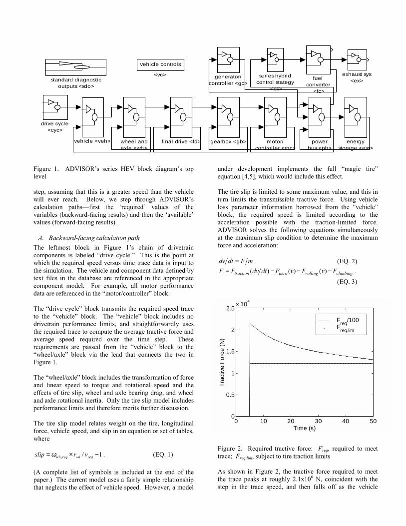
Figure 1. ADVISOR’s series HEV block diagram’s toplevel

step, assuming that this is a greater speed than the vehiclewill ever reach. Below, we step through ADVISOR’scalculation paths—first the ‘required’ values of thevariables (backward-facing results) and then the ‘available’values (forward-facing results).

A. Backward-facing calculation path

The leftmost block in Figure 1’s chain of drivetraincomponents is labeled “drive cycle.” This is the point atwhich the required speed versus time trace data is input tothe simulation. The vehicle and component data defined bytext files in the database are referenced in the appropriatecomponent model. For example, all motor performancedata are referenced in the “motor/controller” block.

The “drive cycle” block transmits the required speed traceto the “vehicle” block. The “vehicle” block includes nodrivetrain performance limits, and straightforwardly usesthe required trace to compute the average tractive force andaverage speed required over the time step. Theserequirements are passed from the “vehicle” block to the“wheel/axle” block via the lead that connects the two inFigure 1.

The “wheel/axle” block includes the transformation of forceand linear speed to torque and rotational speed and theeffects of tire slip, wheel and axle bearing drag, and wheeland axle rotational inertia. Only the tire slip model includesperformance limits and therefore merits further discussion.

The tire slip model relates weight on the tire, longitudinalforce, vehicle speed, and slip in an equation or set of tables,where

1/, −×= reqwhreqwh vrslip ω . (EQ. 1)

(A complete list of symbols is included at the end of thepaper.) The current model uses a fairly simple relationshipthat neglects the effect of vehicle speed. However, a model

under development implements the full “magic tire”equation [4,5], which would include this effect.

The tire slip is limited to some maximum value, and this inturn limits the transmissible tractive force. Using vehicleloss parameter information borrowed from the “vehicle”block, the required speed is limited according to theacceleration possible with the traction-limited force.ADVISOR solves the following equations simultaneouslyat the maximum slip condition to determine the maximumforce and acceleration:

mFdtdv = (EQ. 2)

climbingrollingaerotraction FvFvFdtdvFF −−−= )()()( .

(EQ. 3)

Figure 2. Required tractive force: Freq, required to meettrace; Freq,lim, subject to tire traction limits

As shown in Figure 2, the tractive force required to meetthe trace peaks at roughly 2.1x106 N, coincident with thestep in the trace speed, and then falls off as the vehicle

wheel andaxle <wh>

vehicle <veh>

standard diagnosticoutputs <sdo>

series hybridcontrol stategy

<cs>

powerbus <pb>

motor/controller <mc>

generator/controller <gc>

gearbox <gb>

fuelconverter

<fc>

final drive <fd>

exhaust sys<ex>

energystorage <ess>

drive cycle<cyc>

vehicle controls

<vc>

0 10 20 30 40 500

0.5

1

1.5

2

2.5x 10

4

Time (s)

Tra

ctiv

e F

orce

(N

)

Freq

/100F

req,lim

accelerates to approach the trace. (Figure 3 shows thecalculated vehicle speed.) The maximum tractive force thetires can transmit is constant at roughly 1.2x104 N.

Figure 3. Required and actual vehicle speed

Figure 3 shows the various required vehicle speeds in themodel. The required trace that is output by the “drivecycle” block is shown as vtrace. The average speed requiredover the time step that is output by the “vehicle” block isshown as vreq. The influence of the tire slip model can beseen by comparing vreq with vlim,req, which is the vehiclespeed possible given the tire’s traction limit. Finally, vact isthe vehicle’s actual speed, shown here for reference. Notethat the actual vehicle speed is lower than the tire limitbecause in this example it is limited by the components“upstream” of it.

With tire slip limits enforced, the required wheel speed iscalculated as follows:

( ) .1 ,, whreqlimreqwh rvslip+=ω (EQ. 4)

Required torque input to the axle is computed by summingthe torque required to provide the necessary averagetractive force, the torque required to overcome bearinglosses and brake drag, and the torque required to acceleratethe wheels’ and axles’ rotational inertia.

∆

∆++=

tJrF reqwh

whlosswhwhreqlimreqwh,

,,,

ωττ (EQ. 5)

The “wheel/axle” block sends its torque and speedrequirements to the “final drive” block, which includes nolimits and straightforwardly transforms the torque andspeed requirements with its gear ratio and torque loss. Thenext in line in Figure 1, the “gearbox” block, likewiseincludes no performance limits. After transforming thetorque and speed required of it, the “gearbox” passes therequirements upstream to the “motor/controller” block.

The next section will focus on the motor and motorcontroller model because it enforces a number ofperformance limits, and is perhaps the component modelmost representative of ADVISOR’s hybridbackward/forward approach. Although the motor is not theend of the line of backward-facing calculations inADVISOR, it will be the most ‘upstream’ componentdiscussed in this paper. Discussion of the componentsfurther upstream such as the energy storage system wouldnot significantly further illuminate ADVISOR’s uniqueapproach.

B. Details of motor and motor controller

The top half of ADVISOR’s motor/controller model, shownin Figure 4 in the dashed box, is dedicated to the backward-facing part of the simulation. The required output torqueand speed are input at the top left-hand corner of the blockdiagram, and the required input power is output at the topright-hand corner.

Three different performance limits are enforced in thebackward-facing part of the “motor/controller” block. Therequired speed is limited to the motor’s maximum speed.The required torque is limited to the difference between themotor’s maximum torque at the limited speed and thetorque required to overcome the rotor inertia. The limitedtorque and speed are then used to interpolate in themotor/controller’s input power map. Finally, theinterpolated input power is limited by the motor controller’smaximum current limit. This behavior is described in thefollowing equations:

( )prevbusmaxconmapinmotreqinmot VIPP ,,,,,, ,min= (EQ. 6)

where

( )reqlimmotreqmot,limmapinmot fP ,,,,, ,ωτ= , (EQ. 7)

f is the functional relationship described by the motor map,

( )maxmotreqmotreqlimmot ,,,, ,min ωωω = , (EQ. 8)

and

( )

∆

∆+=

tJf reqlimmot

motreqmotreqlimmotreqlimmot,,

,,,1,, ,minω

τωτ

(EQ. 9)

where f1 is the functional relationship described by themotor’s torque envelope. For cases where the vehiclemissed the required trace by more than 1.6 km/h in theprevious time step, ωmot,lim,req is replaced in Equations 7 and8 and in the f1 function evaluation in Equation 9 by theprevious time step’s actual motor speed, given byEquation 10.

0 10 20 30 40 500

50

100

150

200

250

300

350

Time (s)

Ve

hicle

Sp

ee

d (

km/h

)

vtrace

vreq

vlim,req

vact

Figure 4. ADVISOR’s motor/controller block diagram

prevavail

reqmot,limactprevactmot

vv

= ,

,,

ωω (EQ. 10)

Figure 5 illustrates the effect of Equation 9. In themaximum-effort acceleration example, the motor is askedto produce more than its maximum torque. At times after5 s, the maximum torque capability represented by τmot,lim,req

is used to formulate the motor/controller input powerrequirement.

Figure 5. Required motor torque: τmot,req, required into gearreduction; τmot,lim,req, subject to motor torque limit

Figure 6 illustrates the effect of Equation 8. After about 42s, the motor is required to exceed its maximum speed toprovide the wheel and axle (via a gear reduction) themaximum speed they are capable of handling. ωmot,lim,req,coincident with ωmot,req curve for most of the acceleration, isused to formulate the motor input power requirement.

Figure 6. Required motor speed: ωmot,req, required into gearreduction; ωmot,lim,req, subject to motor speed limit

Figure 7 illustrates the effect of Equation 6. Pmot,in,map is theinput power required to power the motor at its maximum-limited torque and speed. Pmot,in,req is the power that themotor/controller requires of the power bus, which must inturn be provided by the batteries and/or the generator. Forthe example case of a maximum effort acceleration,Figure 7 indicates that between about 9 s and 18 s the motorrequires more power than it is capable of handling,according to its current limit, to meet the limited torque andspeed requirements.

The bottom part of Figure 4, not enclosed in a dashed box,is the forward-facing part of the motor/controller model. Itaccepts as input the available input power, on the bottomleft of the figure, and produces as outputs the availablerotor torque and speed.

2

d ri ve to rq u e a n dsp e e d a va i l . a t ro to r

(N m ), (ra d /s)

1

re q 'd m o to ri n p u t p o we r (W )

rotor drive torqueavailable (Nm)

2-D LookupTable

motor/controllerinput power

map (W)motor speed

estimator

w_mc_out_r

P_mc_in_1lim

P_mc_in_r

motor controllerlogic interfaceenforce

torquelimit

effect of inertia(Nm)

Sum1

Sum

Saturation

N-m drive torqueper W input

Mux

Demux

Demux

2

a va i l a b l e m o to ri n p u t p o we r (W )

1

to rq u e a n d sp e e d re q 'd a t ro to r(N m ), (ra d /s)

0 10 20 30 40 500

200

400

600

800

1000

Time (s)

Mo

tor

Sp

eed

(1

/s)

ωmot,req

ωmot,lim,req

0 10 20 30 40 500

100

200

300

400

500

600

700

Time (s)

Mot

or T

orq

ue (

Nm

)

τmot,req

τmot,lim,req

Figure 7. Required motor/controller input power:Pmot,in,map, computed by map; Pmot,in,req, subject to controllercurrent limit

To compute the torque that can be produced by themotor/controller given the available input power, themotor/controller efficiency computed during the backward-facing calculations is used, modeled as τmot,lim,req/Pmot,lim,req inEquation 11 below.

∆

∆−

=

tJ

P

P reqlimmotmot

reqlimmot

availmotreqlimmotavailmot

,,

,,

,,,,

ωττ

(EQ. 11)

Note that the model accounts for the torque required toaccelerate the motor’s rotor using the motor shaft’srequired acceleration. For maximum-effort accelerationruns, the required acceleration is limited by the tire slip, andthis acceleration is usually greater than what is possiblegiven the drivetrain limits. Therefore, the motor’s inertialeffect is overestimated for maximum-effort accelerationruns. We see below that this overestimation has negligibleeffect on ADVISOR’s fidelity.

The motor speed that the “motor/controller” block outputs,which is termed “available” speed, is the motor’s actualspeed only if there are no torque or power limits activeduring the current time step. Figure 6 indicates that themotor model’s output available speed is equal to ωmot.lim,req

as computed in Equation 8. This means that the “available”motor speed is the required motor speed subject to themotor’s speed limit. If the available motor torque is lessthan the required motor torque, however, there isinsufficient torque for the motor to accelerate to its requiredspeed. This would cause the “available” motor speedoutput by the “motor/controller” block to be greater thanthe actual speed of the motor.

C. Forward-facing calculation path

The available motor torque is transformed by theefficiencies of the gearbox and the final drive (which are

computed during the backward-facing calculations), andtheir gear reductions. This results in available drivetraintorque and speed input to the wheel and axle. Wheel slipplays a role in transforming the available speed only if it isdifferent from the required speed, as is the case if adrivetrain component’s speed limit is encountered. This isdescribed in the equation below:

( )sliprv whavailwhavail += 1,ω , (EQ. 12)

where slip is recomputed here using the available tractiveforce and vavail is the component speed capability-limitedvehicle speed.

Slip plays no role in computing tractive force beyondlimiting the request in the backward-facing calculations.Because no calculation in the upstream components acts toincrease the tractive force, the limit enforced by the slipmodel remains in place through the forward-facingcalculations in the “wheel/axle” block.

After accounting for losses in the axle and dividing by thetire’s rolling radius, ADVISOR arrives at an availabletractive force. Solving Equation 3 for the speed at the endof the time step, ADVISOR arrives at an estimate of theactual vehicle speed. ADVISOR compares this force-basedestimate of vehicle speed with that derived fromEquation 12, and chooses the minimum of the two for theactual vehicle speed, vact, plotted in Figure 3. In this way,the computed vehicle speed never exceeds that possiblegiven the torque and force available from the drivetrain orthe speed that corresponds to any drivetrain componentspeed limits that might be active.

III. EVALUATION OF THE MODEL

A. Accuracy

Having illustrated the mathematical background of thepowertrain model, we can now examine the validity andeffect of the crucial assumption in ADVISOR’s simplifiedforward-facing approach—that is, that actual componentefficiency is closely approximated by that computed in thebackward-facing calculations. This assumption is activeonly when component performance limits areencountered—when they are not, ADVISOR operatesexactly as a strictly backward-facing model. We evaluatethe effects of the crucial assumption by comparingADVISOR’s predictions for a performance-limited case(where the achieved speed falls short of the trace) to thosefor the case where the required trace is equal to the actualvehicle speed. We consider acceleration time and energyuse predictions separately.

1) Simulation parametersRange-extender series hybrid vehicles sized to achieve 0-100 km/h accelerations in 15, 20, and 25 s were simulatedin this test. Their parameters are listed in Table 1.

0 10 20 30 40 500

1

2

3

4

5

6

7x 10

4

Time (s)

Mo

tor/

Co

ntro

ller

Inp

ut P

ow

er

(W)

Pmot,in,map

Pmot,in,req

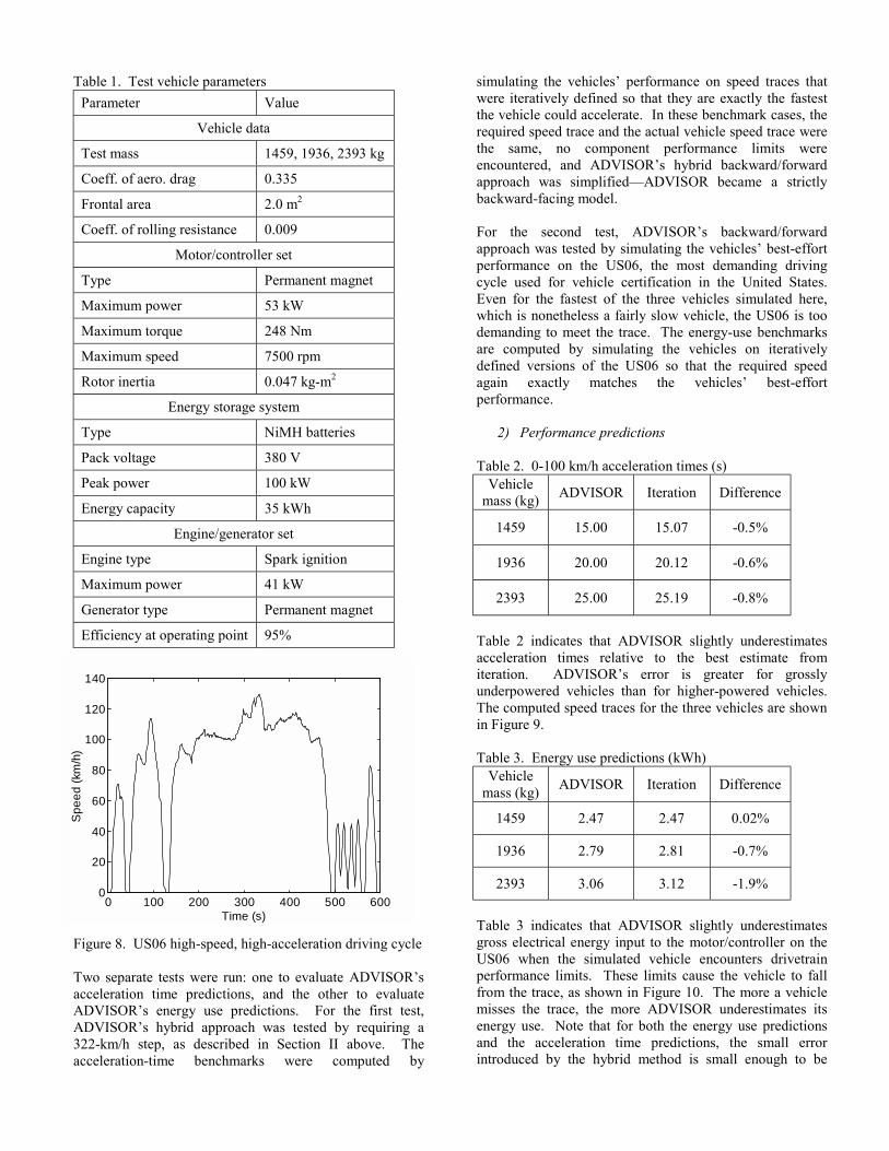
Table 1. Test vehicle parameters

Parameter Value

Vehicle data

Test mass 1459, 1936, 2393 kg

Coeff. of aero. drag 0.335

Frontal area 2.0 m2

Coeff. of rolling resistance 0.009

Motor/controller set

Type Permanent magnet

Maximum power 53 kW

Maximum torque 248 Nm

Maximum speed 7500 rpm

Rotor inertia 0.047 kg-m2

Energy storage system

Type NiMH batteries

Pack voltage 380 V

Peak power 100 kW

Energy capacity 35 kWh

Engine/generator set

Engine type Spark ignition

Maximum power 41 kW

Generator type Permanent magnet

Efficiency at operating point 95%

Figure 8. US06 high-speed, high-acceleration driving cycle

Two separate tests were run: one to evaluate ADVISOR’sacceleration time predictions, and the other to evaluateADVISOR’s energy use predictions. For the first test,ADVISOR’s hybrid approach was tested by requiring a322-km/h step, as described in Section II above. Theacceleration-time benchmarks were computed by

simulating the vehicles’ performance on speed traces thatwere iteratively defined so that they are exactly the fastestthe vehicle could accelerate. In these benchmark cases, therequired speed trace and the actual vehicle speed trace werethe same, no component performance limits wereencountered, and ADVISOR’s hybrid backward/forwardapproach was simplified—ADVISOR became a strictlybackward-facing model.

For the second test, ADVISOR’s backward/forwardapproach was tested by simulating the vehicles’ best-effortperformance on the US06, the most demanding drivingcycle used for vehicle certification in the United States.Even for the fastest of the three vehicles simulated here,which is nonetheless a fairly slow vehicle, the US06 is toodemanding to meet the trace. The energy-use benchmarksare computed by simulating the vehicles on iterativelydefined versions of the US06 so that the required speedagain exactly matches the vehicles’ best-effortperformance.

2) Performance predictions

Table 2. 0-100 km/h acceleration times (s)Vehicle

mass (kg)ADVISOR Iteration Difference

1459 15.00 15.07 -0.5%

1936 20.00 20.12 -0.6%

2393 25.00 25.19 -0.8%

Table 2 indicates that ADVISOR slightly underestimatesacceleration times relative to the best estimate fromiteration. ADVISOR’s error is greater for grosslyunderpowered vehicles than for higher-powered vehicles.The computed speed traces for the three vehicles are shownin Figure 9.

Table 3. Energy use predictions (kWh)Vehicle

mass (kg)ADVISOR Iteration Difference

1459 2.47 2.47 0.02%

1936 2.79 2.81 -0.7%

2393 3.06 3.12 -1.9%

Table 3 indicates that ADVISOR slightly underestimatesgross electrical energy input to the motor/controller on theUS06 when the simulated vehicle encounters drivetrainperformance limits. These limits cause the vehicle to fallfrom the trace, as shown in Figure 10. The more a vehiclemisses the trace, the more ADVISOR underestimates itsenergy use. Note that for both the energy use predictionsand the acceleration time predictions, the small errorintroduced by the hybrid method is small enough to be

0 100 200 300 400 500 6000

20

40

60

80

100

120

140

Spe

ed

(km

/h)

Time (s)

neglected relative to the effect of uncertainty in input dataused to define the simulated vehicle.

Figure 9. Maximum-effort acceleration results for the threeseries hybrids

Figure 10. US06 speed trace deviation, by fastest (topgraph), mid-speed (middle), and slowest (bottom) serieshybrids

The results above were derived using a motor data set thatincludes nonzero inertia, as indicated in Table 1. By settingthis inertia to zero in the model and rerunning the analysesthat produced the results in Tables 2 and 3, we can estimatethe effect of motor inertia on the fidelity of the model.Recall that the iteration method produces correct results(that is, consistent with a backward-facing model’spredictions) regardless of the value of the motor inertiabecause the iteration is performed to ensure that noperformance limits are encountered.

A comparison of Table 4 to the 1936-kg vehicle’s results inTables 2 and 3 indicates that the presence or absence ofmotor inertia does not significantly affect ADVISOR’sagreement with the iteration-derived best estimate.

Table 4. Results for 1936-kg vehicle with zero motorinertia

Performancemeasure

ADVISOR Iteration Diff.

0-100 km/htime (s)

19.76 19.90 -0.7%

Energy input tomotor (kWh)

2.79 2.81 -0.7%

3) Past validation and benchmarkingExercises such as that documented above are instructiveand helpful in confirming ADVISOR’s behavior, but notsufficient to instill confidence that the model is consistentwith other models or real test vehicles. The validation ofADVISOR to ensure its accuracy has been a high prioritysince its initial development. Beginning in 1995, NRELparticipated with representatives from industry and othernational labs in a model benchmarking exercise. When allparticipants used identical inputs, we found thatADVISOR’s predictions closely matched those of industry.When the PNGV Systems Analysis Toolkit (PNGVSAT)version 1.7 became available in April 1997, abenchmarking with that model confirmed similar resultsfrom both models for the cases studied. NREL is currentlyundergoing a benchmarking with a beta versionPNGVSAT 2.1.

In 1997, researchers at Virginia Polytechnic Institutevalidated ADVISOR using data from their award-winningFutureCar competition series hybrid entry. The researchersdeveloped data files representing their vehicle and each ofits components and modified the default control strategy tomatch their own. They then simulated the vehicle’sperformance on the vehicle’s actual speed trace, andcompared the ADVISOR-predicted fuel-use and batteryenergy-use with the measured values. They foundagreement within the uncertainty of their measurements [6].

B. Speed

As mentioned above, backward-facing models tend to befaster than forward-facing models largely because of theway they estimate drivetrain component speeds. Backward-facing models compute the speeds directly from therequired vehicle speed trace, whereas forward-facingmodels integrate a = F / m to compute speeds. Thisapproach requires the use of higher order integrationschemes and smaller time steps.

ADVISOR handles drivetrain speeds much in the same waythat strictly backward-facing models do, and is thereforesignificantly faster than typical forward-facing models.Table 5 compares ADVISOR’s execution times to those ofa proprietary Simulink-based forward-facing model.ADVISOR and the forward-facing model were both used tosimulate a conventional-drivetrain vehicle, and were run onthe same 200-MHz Intel Pentium Pro-equipped personalcomputer running Microsoft Windows 95.

0 5 10 15 20 250

20

40

60

80

100

Time (s)

Spe

ed (k

m/h

)

ADVISORIteration

0 100 200 300 400 500 6000

10

20

Spe

ed (k

m/h

)

0 100 200 300 400 500 6000

10

20

Spe

ed (k

m/h

)

0 100 200 300 400 500 6000

10

20

Spe

ed (k

m/h

)

Time (s)

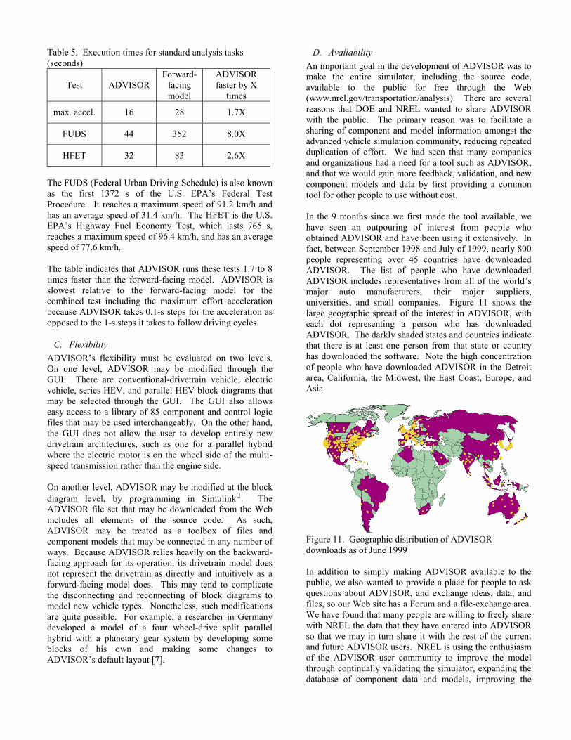
Table 5. Execution times for standard analysis tasks(seconds)

Test ADVISORForward-

facingmodel

ADVISORfaster by X

times

max. accel. 16 28 1.7X

FUDS 44 352 8.0X

HFET 32 83 2.6X

The FUDS (Federal Urban Driving Schedule) is also knownas the first 1372 s of the U.S. EPA’s Federal TestProcedure. It reaches a maximum speed of 91.2 km/h andhas an average speed of 31.4 km/h. The HFET is the U.S.EPA’s Highway Fuel Economy Test, which lasts 765 s,reaches a maximum speed of 96.4 km/h, and has an averagespeed of 77.6 km/h.

The table indicates that ADVISOR runs these tests 1.7 to 8times faster than the forward-facing model. ADVISOR isslowest relative to the forward-facing model for thecombined test including the maximum effort accelerationbecause ADVISOR takes 0.1-s steps for the acceleration asopposed to the 1-s steps it takes to follow driving cycles.

C. Flexibility

ADVISOR’s flexibility must be evaluated on two levels.On one level, ADVISOR may be modified through theGUI. There are conventional-drivetrain vehicle, electricvehicle, series HEV, and parallel HEV block diagrams thatmay be selected through the GUI. The GUI also allowseasy access to a library of 85 component and control logicfiles that may be used interchangeably. On the other hand,the GUI does not allow the user to develop entirely newdrivetrain architectures, such as one for a parallel hybridwhere the electric motor is on the wheel side of the multi-speed transmission rather than the engine side.

On another level, ADVISOR may be modified at the blockdiagram level, by programming in Simulink . TheADVISOR file set that may be downloaded from the Webincludes all elements of the source code. As such,ADVISOR may be treated as a toolbox of files andcomponent models that may be connected in any number ofways. Because ADVISOR relies heavily on the backward-facing approach for its operation, its drivetrain model doesnot represent the drivetrain as directly and intuitively as aforward-facing model does. This may tend to complicatethe disconnecting and reconnecting of block diagrams tomodel new vehicle types. Nonetheless, such modificationsare quite possible. For example, a researcher in Germanydeveloped a model of a four wheel-drive split parallelhybrid with a planetary gear system by developing someblocks of his own and making some changes toADVISOR’s default layout [7].

D. Availability

An important goal in the development of ADVISOR was tomake the entire simulator, including the source code,available to the public for free through the Web(www.nrel.gov/transportation/analysis). There are severalreasons that DOE and NREL wanted to share ADVISORwith the public. The primary reason was to facilitate asharing of component and model information amongst theadvanced vehicle simulation community, reducing repeatedduplication of effort. We had seen that many companiesand organizations had a need for a tool such as ADVISOR,and that we would gain more feedback, validation, and newcomponent models and data by first providing a commontool for other people to use without cost.

In the 9 months since we first made the tool available, wehave seen an outpouring of interest from people whoobtained ADVISOR and have been using it extensively. Infact, between September 1998 and July of 1999, nearly 800people representing over 45 countries have downloadedADVISOR. The list of people who have downloadedADVISOR includes representatives from all of the world’smajor auto manufacturers, their major suppliers,universities, and small companies. Figure 11 shows thelarge geographic spread of the interest in ADVISOR, witheach dot representing a person who has downloadedADVISOR. The darkly shaded states and countries indicatethat there is at least one person from that state or countryhas downloaded the software. Note the high concentrationof people who have downloaded ADVISOR in the Detroitarea, California, the Midwest, the East Coast, Europe, andAsia.

Figure 11. Geographic distribution of ADVISORdownloads as of June 1999

In addition to simply making ADVISOR available to thepublic, we also wanted to provide a place for people to askquestions about ADVISOR, and exchange ideas, data, andfiles, so our Web site has a Forum and a file-exchange area.We have found that many people are willing to freely sharewith NREL the data that they have entered into ADVISORso that we may in turn share it with the rest of the currentand future ADVISOR users. NREL is using the enthusiasmof the ADVISOR user community to improve the modelthrough continually validating the simulator, expanding thedatabase of component data and models, improving the

functionality and usability of the simulator, and ultimatelyfeeding this back to the ADVISOR users.

E. Ease of use

Because we knew the potential users of ADVISOR 2.1would have diverse backgrounds, we had to make themodel easy to use so it would be accessible to such a largeaudience. Having a powerful and user-friendly GUI wasthe key to enabling ADVISOR to reach out to a broadaudience and enable people to effectively answer vehiclesystems analysis questions of their own. NREL wrote theGUI in the latest MATLAB®/Simulink® environment, and itenables straightforward access to many powerful analysisfunctions. The following descriptions of the three mainGUI pages explain the wide array of features that areavailable for configuring a vehicle, conducting asimulation, and analyzing the results.

1) Vehicle Input PageThe layout of this screen is typical of all three GUI screens,in that the left-hand side of the window is the graphicalrepresentation of vehicle information and the right-handside is where the user takes action. On the right-hand sideof the screen, the user specifies what he wants to see and doto the vehicle, and controls the next action for ADVISOR totake. For example, on the vehicle input screen (seeFigure 12), the picture in the upper left serves as a graphicalindication of which vehicle configuration has been selected(conventional, series, parallel, fuel cell, or electric vehicle).The user-selectable graphs in the lower left allow the userto immediately view the performance information on thecomponents that have been selected, such as efficiencycontours for the engine and motor, emissions contours, andperformance graphs for the batteries.

Figure 12. ADVISOR 2.1 vehicle input screen

On the right-hand portion of the vehicle input screen, theuser controls what type of vehicle is simulated and thedetails of all the components that make up the drive system.Each component has a pull-down menu that allows differentcomponents to be selected from the ADVISOR library. The

two columns of numbers under the “maximum power” and“peak efficiency” headings initially indicate these valuesfrom the data files, but typing in a new number causes theGUI to linearly rescale the entire efficiency map to matchthat peak efficiency while preserving the map’s originalshape. For example, entering in a 0.45 rather than theexisting 0.42 in the engine peak efficiency would allow theuser to examine the impact of a hypothetical engine thatcould achieve a 45% peak efficiency rather than 42%.

Just above these columns is an “autosize” button thatsimplifies the task of iteratively sizing drivetraincomponents (engine, motor, and batteries) to meet userdefined minimum performance requirements of accelerationand gradability. For parallel vehicles, the autosize functionalso allows the user to select the degree of hybridization,which is reflected in the relative sizing of the engine, motor,and batteries.

Finally, the user can modify any scalar parameter thatADVISOR defines on the MATLAB® workspace throughthe variable list. Because the total vehicle test mass is aparameter that is often desirable to override in various“what-if” scenarios, it is brought to the top level and can beoverridden with a single mouse click and by entering thenew mass. Vehicle input files can also be saved; they storethe names of the component files selected and all scalingand override settings to allow the user to recreate results ata future time or share input settings with a colleague.

2) Simulation Setup PageThe second of the three ADVISOR 2.1 GUI screens is theSimulation Setup screen (Figure 13). The primary decisionfor the user on this screen is whether to run a single cycle(and which one) or a test procedure, which can consist ofspecial initial conditions, multiple cycles, and significantpost-processing (such as the test procedure to determinecombined city/highway fuel economy).

If the single cycle option is chosen, initial conditions(primarily thermal and battery) can be set, and for hybridsthe type of battery state of charge (SOC) correction routinecan also be selected. The two SOC correction optionsavailable are a zero-delta or a linear correction routine. Thezero-delta routine iterates on the initial SOC until the finalSOC is within some tolerance (0.5%) of it. The linearcorrection routine starts the battery at both its extreme highand low SOC, and then performs a linear interpolation toestimate the fuel economy at the zero-delta SOC crossing.Additionally, gradability and acceleration tests can beselected for evaluation.

Finally, because parametric studies are often useful toexplore the design space of a given vehicle, ADVISOR 2.1allows the option of doing a 1-, 2-, or 3-parameter designsweep of any scalar value on the workspace. This allowsthe sensitivity of a vehicle to its various input parameters tobe evaluated, not only on fuel economy, but also onperformance.

Figure 13. ADVISOR 2.1 simulation setup screen

3) Results PageThe Results Page (Figure 14) is the last of the three majorADVISOR screens. This page allows the user to see thesummary results of fuel economy, emissions, acceleration,and gradability on the right-hand side, and plots of any ofthe time-dependent variables that the simulation puts ontothe workspace on the left-hand side.

Figure 14. ADVISOR 2.1 Results Screen

The results screen has separate pop-up windows if testprocedures or parametric studies are selected rather thansingle cycles. ADVISOR 2.1 allows full usage of the built-in plotting features of MATLAB® including zoom, layeringmultiple curves on the same graph, and applying gridlines.In Figure 14, which shows a sample results screen, you cansee four representative plots: vehicle speed, battery SOC,regulated emissions, and temperatures at various placeswithin the exhaust system.

There are two action buttons that pull up an energy usagefigure and a series of diagnostic plots. The energy usagefigure tracks all the energy through the drivetrain, noteswhere it is used, and performs an energy balance to make

sure that there is no unaccounted-for energy. On allscreens, there is a ‘HELP’ button that takes the user directlyto the browser-viewable documentation for moreinformation.

Feedback from our users indicates that we have beensuccessful in creating a program that is easy to use andallows reasonably novice users to produce useful results aspart of their vehicle systems analysis studies.

IV. CONCLUSIONS

The mathematical background behind ADVISOR 2.1,which uses a unique combined backward/forward facingapproach, has been illustrated. The model and overallapproach has been evaluated relative to the NREL team’sobjectives, which include accuracy, speed, flexibility,availability, and ease of use.

- Accuracy: For three vehicles ranging in 100 km/hacceleration time from 15 to 25 s, ADVISOR predictsto within 0.8% the acceleration time computed byiteration. Energy use on the US06 is predicted towithin 1.9%, even for extremely underpoweredvehicles that push the assumptions of ADVISOR’sapproach. For typical vehicles simulated, the energypredictions are within 0.02%.

- Speed: ADVISOR is 2.6 to 8.0 times faster than acomparable Simulink®-based forward-facing vehicleperformance simulator in the tests documented here.

- Flexibility: The ADVISOR library contains numerousinterchangeable component data files that may be usedin a number of drivetrain configurations. It may bechallenging to develop completely new drivetrainconfiguration models, but many ADVISOR users havealready done this successfully.

- Availability: ADVISOR is available on the Web andhas been downloaded by an international group of over800 users representing over 45 countries.

- Ease of use: ADVISOR 2.1 includes a powerful GUIto allow even novice users to quickly analyze vehiclepowertrains.

SYMBOLS

F force, NI current, AJ rotational inertia, kg-m2

m mass, kgP power, Wr radius, mt (simulation) time, sv vehicle speed, m/sV voltage, Vτ torque, N-mω rotational speed, s-1

SUBSCRIPTS

act actualavail available—possible given the drivetrain limitscon associated with the motor controllerlim subject to a component performance limitmap computed from component performance mapmot associated with the motor or motor/controller setprev computed in the previous time stepreq requiredwh associated with the wheel or wheel & axle

ACKNOWLEDGMENT

The authors gratefully acknowledge the continued supportof the U.S. Department of Energy for vehicle systemsanalysis at NREL.

REFERENCES

[1] Cole, G. H., “SIMPLEV: A Simple Electric Vehicle SimulationProgram, Version 2.0.” EG&G Idaho, Inc. April 1993.

[2] “The AeroVironment Electric/Hybrid Vehicle Simulator, CarSim2.5.4, Desktop Version, Documentation.” AeroVironment, Inc.Monrovia, CA. August, 1994.

[3] Murrell, J. D., “Vehicle Powertrain Modeling,” Letter Report underConsultant Agreement CCD-4-1403-01 to NREL, March 1995.

[4] Gillespie, T. D., Fundamentals of Vehicle Dynamics, published bySociety of Automotive Engineers, Warrendale, PA, 1992.

[5] Bakker, E., H. B. Pacejka, L. Lidner, “A New Tire Model with anApplication in Vehicle Dynamics Studies,” SAE Technical PaperNumber 890087, 1989.

[6] Senger, R. D., M. A. Merkle, D. J. Nelson, “Validation of ADVISORas a Simulation Tool for a Series Hybrid Electric Vehicle,”Technology for Electric and Hybrid Vehicles, Proceedings of the1998 SAE Intl. Congress, Detroit, MI, Feb. 23-26, SAE Paper No.981133, SP-1331, pp. 95-115, 1998.

[7] Santoro, M., “A Hybrid-Propulsion Powertrain with Planetary GearSet for a 4WD Vehicle: Analysis of Power Flows and EnergyEfficiency,” 54th ATI (Associazione Termotecnica Italiana) NationalCongress, September 14-17, 1999, L’Aquila, Italy.

Keith B. Wipke holds a B.S. in mechanicalengineering from the University of California,Santa Barbara, and an M.S.M.E. from StanfordUniversity. He has worked at NREL since 1991,on activities such as testing and data collectionfrom electric and hybrid vehicles and buses,computer modeling and optimization of hybridvehicles using ADVISOR, and thermal andelectric testing of hybrid electric vehicle batteries.He is currently the team leader for NREL’s

vehicle systems analysis team, which improves and maintains theADVISOR advanced vehicle simulator.

Matthew R. Cuddy holds a B.S.M.E. fromCornell University and an M.S.M.E. from theUniversity of Colorado. In 1992 and 1993, hedeveloped models of turbulent diffuser and roomairflow for buildings applications at NREL. From1994 to 1998 he studied hybrid vehiclepowertrain performance at NREL, developingADVISOR in 1994. He is currently analyzingand developing new powertrain components andvehicle auxiliary load reduction systems as aconsultant based in Amherst, Massachusetts.

Steven D. Burch holds an M.S.M.E. from PurdueUniversity. Before joining NREL in 1992, hespent 4 years with Delphi - Harrison ThermalSystems (General Motors) as a project engineer inheat exchanger R&D. In his tenure at NREL, hedeveloped numerous models of thermal systemsin buildings and automobiles and also developedthermal management systems for batteries andcatalytic converters. He was project leader forwork with Benteler Automotive, Inc., to developa practical vacuum-insulated automotive catalytic

converter on which he holds a patent. He has recently joined GeneralMotors’ fuel cell division.