Advertising Dynamics and Competitive Advantage∗

Ulrich DoraszelskiHoover Institution, Stanford University†

Sarit MarkovichRecanati Graduate School of Business Administration, Tel Aviv University‡

November 2, 2003

Abstract

Can advertising lead to a sustainable competitive advantage? To answer this ques-tion, we propose a dynamic model of advertising competition where firms repeatedlyadvertise, compete in the product market, and make entry as well as exit decisions.Within this dynamic framework, we study two different models of advertising: In thefirst model, advertising influences the goodwill consumers extend towards a firm (“good-will advertising”), whereas in the second model it influences the share of consumers whoare aware of the firm (“awareness advertising”). We show that asymmetries may ariseand persist under goodwill as well as awareness advertising. The basis for a strategicadvantage, however, differs greatly in the two models of advertising. We show thattighter regulation or an outright ban of advertising may have anticompetitive effectsand discuss how firms use advertising to deter and accommodate entry and induce exitin a dynamic setting.

1 Introduction

Consider two ex ante identical firms that each invest in an advertising campaign. Supposesheer luck has it that one advertising campaign is successful while the other is not. Thencertainly today the lucky firm will be in a better position than its unlucky rival. But will itbe able to sustain its competitive advantage tomorrow? That is, will the difference betweenthe firms tend to increase or decrease as time passes?

The existing dynamic models of advertising competition suggest the latter: Thereis a globally stable symmetric steady state (see e.g. Friedman 1983, Fershtman 1984,

∗An earlier version of this paper was circulated under the title “Goodwill and Awareness Advertising:Implications for Industry Dynamics.” We thank Lanier Benkard, David Besanko, Jeremy Bulow, RobertClark, Michaela Draganska, Chaim Fershtman, David Genesove, Wes Hartmann, Heidrun Hoppe, Ken Judd,Patricia Langohr, Jim Lattin, Volker Nocke, Rob Porter, Uday Rajan, Mark Satterthwaite, Katja Seim,Frank Stahler, Victor Tremblay, and Huseyin Yildirim for helpful comments and suggestions.

†Stanford, CA 94305-6010, U.S.A., doraszelski@hoover.stanford.edu.‡Ramat Aviv, Tel Aviv 69978, Israel, saritm@post.tau.ac.il.

1

Chintagunta 1993, Cellini & Lambertini 2003).1 Consequently, any differences among firmsare bound to vanish over time, and there is no room for a sustainable competitive advantage.This is the case even if firms enter the market one by one and thus differ in their strategicpositions at the outset of the game (Fershtman, Mahajan & Muller 1990). In contrast,we provide conditions under which persistent differences arise for strategic reasons as anequilibrium phenomenon among ex ante identical firms.

We propose a dynamic model of advertising competition that adapts the Markov-perfect-equilibrium framework presented in Ericson & Pakes (1995) to track the evolution of anindustry. In particular, we allow firms to advertise on an ongoing basis and to competerepeatedly in the product market, where consumers choose between the differentiated prod-ucts on offer. In addition to making advertising and pricing decisions, incumbent firmsdecide whether to remain in the industry and potential entrants decide whether to enter.Within this dynamic framework, we first specify how advertising affects consumers andbuild up a model of product market competition. We then solve numerically for the sym-metric Markov perfect equilibrium (MPE) in order to characterize industry dynamics andidentify circumstances under which asymmetric industry structures arise and persist overtime.

To study the implications of advertising for industry dynamics, we first need to under-stand the way in which advertising affects consumers. The literature (see Bagwell (2002)for a survey) has traditionally emphasized the persuasive nature of advertising: Its purposeis to alter consumers’ tastes for established brand names or company reputations (Dixit &Norman 1978). On the other hand, Stigler & Becker (1977) and Becker & Murphy (1993)argue that advertising is part of consumers’ preferences in the same way as goods and thatthere are complementarities between advertising and goods. Hence, a more-advertised goodis ceteris paribus preferred over a less-advertised good. Common to the persuasive and thecomplementary view is that advertising affects the utility derived from consuming a partic-ular product. We capture this idea in a model of goodwill advertising. Following Nerlove& Arrow (1962), we take goodwill to be a stock related to the flow of current and pastadvertisements. This stock depreciates over time, reflecting the loss in effectiveness of pastadvertising campaigns. A firm therefore advertises in order to keep up its stock of goodwillas well as to add to it.

Another strand of the literature views advertising as information: Advertising aids theoperation of markets by helping to identify buyers and sellers or by making the terms of saleknown (Stigler 1961). This is especially important in markets for differentiated products

1To be precise, the steady state is symmetric provided that the economic fundamentals are the sameacross firms. Of course, a competitive advantage can arise and persist in a game in which firms differ intheir economic fundamentals (e.g., cost structures). However, rather than explaining asymmetries, this begsthe question how such differences in “initial conditions” come about in the first place.

2

because, if products are differentiated, a consumer may be unaware of the very existenceof a particular product unless she sees it advertised. We capture this informative role ofadvertising in a model of awareness advertising, where advertising influences the share ofconsumers who know about the firm and its product (Grossman & Shapiro 1984, Fershtman& Muller 1993, Boyer & Moreaux 1999).2

The informative role of advertising has previously been analyzed using static models.However, static models cannot tell us anything about whether or not a competitive advan-tage persists. Moreover, they suggest that a competitive advantage does not even arise inthe first place. Butters (1977), Stegeman (1991), and Robert & Stahl (1993) study priceadvertising in markets for homogenous goods. Although the equilibrium in these models ischaracterized by price dispersion, all firms make zero profits and none has a competitiveadvantage. Turning to differentiated products and awareness advertising, no asymmetriesarise in the equilibrium of Grossman & Shapiro’s (1984) model. On the other hand, Fersht-man & Muller (1993) and Boyer & Moreaux (1999) show in the context of a static game ofawareness choice followed by price competition that firms may opt for less than full aware-ness even if advertising were costless. Yet, they are silent as to whether the equilibriumoutcome is going to be symmetric or asymmetric.

In contrast to its informative role, the persuasive role of advertising has already beenanalyzed using dynamic models. Our model of goodwill advertising improves upon earlierwork in a number of ways.3 First, the existing dynamic games either abstract from productmarket competition altogether by assuming a constant markup (Fershtman 1984, Fershtmanet al. 1990, Chintagunta 1993) or use a reduced-form demand specification that depends onstocks of goodwill in a somewhat arbitrary (linear-quadratic) fashion (Friedman 1983, Cellini& Lambertini 2003). In contrast, we start with consumer behavior and derive the model ofproduct market competition. This enables us to specify in more detail why and how goodwilladvertising affects consumer choice. Second, the recent literature on models of industryevolution points out the important role that idiosyncratic shocks play in explaining thegreat variation in the fate of similar firms over time (Jovanovic 1982, Hopenhayn 1992). Weincorporate this insight by making the law of motion of a firm’s stock of goodwill stochastic,whereas existing dynamic games are deterministic. Third, we compute the MPE rather than

2We restrict attention to directly informative advertising. In contrast, building on earlier work by Nelson(1974), Kihlstrom & Riordan (1984) and Milgrom & Roberts (1986), among others, analyze advertising forexperience goods rather than search goods. In this context, advertising is indirectly informative becauseconsumers draw inferences about a product merely from the fact that the firm spends on advertising.Advertising may also signal information about firms themselves. For example, a firm may use advertisingto signal its low cost and the associated low price (Bagwell & Ramey 1994a, Bagwell & Ramey 1994b).

3The literature has traditionally taken a number of shortcuts to modelling dynamic advertising competi-tion, including hazard rate models, passive rival models, and reaction function models. Only recently havedynamic games been developed (see Chapter 11 of Dockner, Jorgensen, Van Long & Sorger (2000) for asurvey).

3

the open-loop equilibrium. As is well known, open-loop equilibria may be based on threatsand promises that are not credible and hence in general fail to be subgame perfect. Fourth,we incorporate entry and exit as key drivers of industry evolution (see e.g. Dunne, Roberts& Samuelson 1988).

For each model of advertising we compute the MPE and analyze the evolution of theindustry. We show that, under goodwill as well as awareness advertising, asymmetries ariseand persist provided that one firm has a strategic advantage over the other. The tangibleform of this advantage is that one firm can deter the other from advertising. The basis fora strategic advantage, however, differs markedly in the two models of advertising.

Under goodwill advertising, the size of the market and the cost of advertising are keydeterminants of industry structure and dynamics. In particular, goodwill advertising leadsto an extremely asymmetric industry structure with a large and a small firm if the marketis small or if advertising is expensive. Because the marginal benefit of advertising is smallrelative to its cost, a small firm has only a weak incentive to advertise when competingagainst a large firm and, in fact, may choose not to advertise at all. If the market is largeor if advertising is cheap, on the other hand, even a small firm has a fairly strong incentiveto advertise. In this case we obtain a symmetric industry structure with two large firms.

In contrast to the cost/benefit considerations that give rise to a strategic advantageunder goodwill advertising, whether or not asymmetries arise and persist under awarenessadvertising depends on the intensity of product market competition. If competition is soft,the industry evolves towards a symmetric structure, but it evolves towards an asymmetricstructure if competition is fierce. Industry dynamics in this latter case resemble a ratherbrutal preemption race. During this race, both firms advertise heavily as long as they areneck-and-neck. Once one of the firms manages to pull even slightly ahead, however, itsrival “gives up,” thereby propelling the firm into a position of dominance. The ensuingasymmetric industry structure persists because it is in the self-interest of the smaller firmto stay behind. In fact, the nature of product market competition is such that once thesmaller firm tries to grow, the larger firm responds aggressively by triggering a “price war,”thereby pushing prices and hence profits down. This gives the smaller firm an overwhelmingincentive to remain inconspicuous.

Our results yield novel insights into the link between advertising restrictions and in-dustry concentration. Whereas the market power theory of advertising (Kaldor 1950, Bain1956, Comanor & Wilson 1974) holds that restricting persuasive advertising aids competi-tion, we show that tighter regulation or an outright ban of goodwill advertising may haveanticompetitive effects. The key insight here is that regulating or banning advertising makesit harder and thus costlier for firms to reach consumers. Given that asymmetries are rootedin cost/benefit considerations in the case of goodwill advertising, this may pave the way for

4

one firm to dominate the industry. Our results are consistent with the empirical finding thatconcentration has increased after regulation was implemented in industries like cigarettes(see, e.g., Eckard 1991) and beer (Sass & Saurman 1995), where advertising is arguablypersuasive rather than informative in nature.

Our dynamic framework also lends itself to studying the role of advertising as a barrierto entry. Contrary to the contention of the literature (Schmalensee 1983, Fudenberg &Tirole 1984), an incumbent deters entry by over-advertising and, in general, accommodatesentry by under-advertising. The reason is that over-advertising makes product market com-petition fiercer in our model of awareness advertising, whereas under-advertising softens it.The incumbent’s desire to soften product market competition, however, may be overriddenby a purely dynamic consideration. If post-entry industry dynamics take the form of a pre-emption race, then the incumbent accommodates the entrant by over-advertising in a bidto gain a head start in the race and in this way improve its chances of eventually becomingthe dominant player in the industry. Taking industry dynamics into account is thus crucialto analyzing barriers to entry.

In sum, this paper bridges the gap between the “micro foundations” of advertising com-petition and the existing dynamic games. By starting with consumer behavior and buildingup a model of product market competition, we are able to study different models of adver-tising while holding consumers’ preferences constant. We do not restrict ourselves to thepersuasive aspects of advertising, but are the first to study its informative aspects in a dy-namic setting. This allows us to shed new light on sources of asymmetries in dynamic modelsof advertising competition. Understanding the mechanisms behind persistent asymmetrieshas important implications for regulatory policy and, in turn, aids our understanding of therole of advertising as a barrier to entry.

The remainder of this paper is organized as follows: We set up the basic model withoutentry and exit in Section 2. We present our results in Section 3. In Section 4 we discussthe link between advertising restrictions and industry concentration. In Section 5 we studyfirms’ entry and exit decisions and their impact on the structure of an industry. Section6 presents a number of robustness checks and an alternative interpretation of the model.Section 7 summarizes and concludes.

2 Model

The model is cast in discrete time and has an infinite horizon to avoid end effects. Thereare two firms with potentially different levels of goodwill or awareness. Each firm is in turnable to influence its goodwill (awareness) level through advertising.

5

Setup and timing. We assume that the goodwill consumers extend towards a firm is atone of L levels and set −∞ < v0 < v1 < . . . < vL−1 < ∞. Similarly, the share of consumerswho are aware of the firm is at one of L levels 0 ≤ s0 < s1 < . . . < sL−1 ≤ 1. In eachperiod, a firm decides how much to advertise in order to add to its goodwill (awareness).At the same time consumers forget, and the firm is bound to lose some of its goodwill(awareness). In other words, goodwill (awareness) decays. The outcomes of the advertisingand forgetting processes are assumed to be stochastic. Thus, even if a firm advertises, itis not guaranteed that its goodwill (awareness) increases. Moreover, the firm’s goodwill(awareness) might decrease due to forgetting despite advertising.

After making their advertising decisions but before the outcomes of the advertising andforgetting processes are realized, firms compete in the product market. Profits from productmarket competition in each period are determined by firms’ levels of goodwill (awareness)(vi, vj) ((si, sj)). To simplify notation we take (i, j) to mean that firm 1’s level of goodwill(awareness) is vi (si) and firm 2’s level of goodwill (awareness) is vj (sj), and denote theprofit functions of firm 1 and firm 2 by π1(i, j) and π2(i, j), respectively. We first providedetails on the product market game under goodwill advertising and then under awarenessadvertising. Finally, we turn to the dynamic framework. We present the derivations forfirm 1, the derivations for firm 2 are analogous.

Goodwill advertising. Suppose that firms’ levels of goodwill are (vi, vj). Taking theirgoodwill levels as given, firms compete in the product market by setting prices (p1, p2). Aconsumer purchases at most one good. The utility consumer m derives from purchasingfrom firm 1 is

vi − p1 + εm1,

where εl1 represents taste differences among consumers. Note that the utility differencebetween consuming and not consuming good 1, (vi − p1 + εm1)−0, is increasing in vi. Thisspecification thus implies that advertising and goods are complementary in the sense ofBecker & Murphy (1993).

Besides the two goods offered by the two firms, there is an outside good, good 0, whichhas utility εm0. In this way we allow advertising to have a market-size effect in addition toa market-share effect (see e.g. Roberts & Samuelson (1988) and Slade (1995) for empiricalevidence).

Assuming that the idiosyncratic shocks εm0, εm1, and εm2 are independently and identi-cally extreme value distributed, the probability that a randomly chosen consumer purchasesfrom firm 1 is

D1(p1, p2; i, j) =exp (vi − p1)

1 + exp (vi − p1) + exp (vj − p2).

6

The profit-maximization problem of firm 1 is thus given by

maxp1≥0

MD1(p1, p2; i, j)p1

where M > 0 is the size of the market (the measure of consumers) and, in the interestof parsimony, we abstract from marginal and fixed costs of production. The first-ordercondition (FOC) is

0 = 1− 1 + exp (vj − p2)1 + exp (vi − p1) + exp (vj − p2)

p1.

It can be shown that there exists a unique Nash equilibrium (p∗1(i, j), p∗2(i, j)) of the

product market game (Caplin & Nalebuff 1991). The Nash equilibrium can be computedeasily by numerically solving the system of FOCs. The per-period profit of firm 1 in theNash equilibrium of the product market game under goodwill advertising is then given byMπ1(i, j), where

π1(i, j) ≡ D1(p∗1(i, j), p∗2(i, j); i, j)p

∗1(i, j) (1)

is the profit per consumer.

Awareness advertising. While the above model emphasizes the persuasive aspects ofadvertising, advertising is informative in our next model. Our product market game underawareness advertising is similar to Fershtman & Muller (1993) and Boyer & Moreaux (1999).

Suppose that firms’ levels of awareness are given by (si, sj). Since we now assume thatadvertising influences awareness rather than goodwill, the utility that consumer m derivesfrom good 1 becomes

v − p1 + εm1.

We refer to v as the perceived quality of firms’ products in order to clearly distinguish itfrom their levels of goodwill in the model of goodwill advertising. Note that the consumerperceives the products of both firms to be of the same quality, reflecting the informativenature of advertising. There is again an outside good, which has utility εm0.

All consumers are aware of the outside good. In addition, a share si of consumers isaware of firm 1 and a share sj of consumers is aware of firm 2. Depending on their choice set,consumers can therefore be divided into four mutually exclusive and exhaustive segments:a group that is aware of neither good 1 nor good 2, a group that is aware of good 1 but notgood 2, a group that is aware of good 2 but not good 1, and a group that is aware of bothgoods.

Assuming that consumers are exposed to advertising at random, the event of beingaware of firm 1 is independent of the event of being aware of firm 2. Hence, the probabilitythat a randomly chosen consumer belongs to the four segments is (1−si)(1−sj), si(1−sj),

7

(1 − si)sj , and sisj , respectively. It follows that the probability that a randomly chosenconsumer purchases from firm 1 is

D1(p1, p2; i, j) = si(1− sj)exp (v − p1)

1 + exp (v − p1)+ sisj

exp (v − p1)1 + exp (v − p1) + exp (v − p2)

. (2)

Equation (2) shows that firm 1’s demand is composed of a captive segment of consumerswho do not know of firm 2 and a competitive segment of consumers who know of firm 2.The size of these segments is proportional to 1− sj and sj , respectively. Moreover, as theperceived quality v goes up, the inside goods become more attractive relative to the outsidegood to both segments of consumers, and competition thus intensifies.

The FOC arising from firm 1’s profit-maximization problem is

0 = (1− sj)exp (v − p1)

1 + exp (v − p1)

(1− 1

1 + exp (v − p1)p1

)

+sjexp (v − p1)

1 + exp (v − p1) + exp (v − p2)

(1− 1 + exp (v − p2)

1 + exp (v − p1) + exp (v − p2)p1

).

In general, there may not be a Nash equilibrium in pure strategies.4 However, byverifying that none of the two firms has a profitable unilateral deviation, it is easy to ensurethat a numerical solution to the system of FOCs constitutes a Nash equilibrium. The per-period profits are then constructed in the same way as in the model of goodwill advertising(equation (1)).

State-to-state transitions. We now turn to the dynamic framework. Recall that we take(i, j) to mean that firm 1’s goodwill (awareness) is vi (si) and firm 2’s goodwill (awareness)is vj (sj). Hence, the industry is completely described by the tuple (i, j) ∈ {0, . . . , L− 1}2.We call (i, j) the state of the industry. Given that the industry is in state (i, j) today, itwill be in state (i′, j′) tomorrow. Our next task is to specify the probability distributionthat governs the state-to-state transitions.

Consider firm 1. Its transition between goodwill (awareness) levels depends on howmuch it advertises and on how easily consumers forget. We think of the advertising andforgetting processes as follows: In each period, firm 1 invests kx1 in an advertising campaign,where x1 ≥ 0 is the amount of advertising and k > 0 measures the cost of advertising. Themore a firm advertises, the higher is the probability that its campaign succeeds in creatinggoodwill (awareness). In particular, we take the probability of success to be x1

1+x1. At

4Note that a firm faces a choice between setting a low price in order to be competitive and exploitingits captive segment by setting a high price. This may give rise to a discontinuity in the firm’s best replyfunction and ultimately lead to nonexistence of a Nash equilibrium in pure strategies. Our computationssuggest that this actually happens for high values of v.

8

the same time, consumers may forget and the firm may thus lose some of its goodwill(awareness). Forgetting can occur when the effect of past advertising on consumers wearsout and is not reinforced by current advertising, when the current advertising campaignis ill-conceived and repels instead of attracts consumers, or when the firm suffers a publicrelations mishap. We take the probability of forgetting to be δ.

Hence, if Pr(i′|i, x1) denotes the probability that firm 1 will be in state i′ tomorrowgiven that it is in state i today, then we have

Pr(i′|i, x1) =

(1−δ)x1

1+x1if i′ = i + 1,

1−δ+δx11+x1

if i′ = i,δ

1+x1if i′ = i− 1

if i ∈ {1, . . . , L−2}. Clearly, firm 1 cannot move further down (up) from the lowest (highest)state. We therefore set

Pr(i′|i, x1) =

{x1

1+x1if i′ = i + 1,

11+x1

if i′ = i

if i = 0, and

Pr(i′|i, x1) =

{1−δ+x11+x1

if i′ = i,δ

1+x1if i′ = i− 1

if i = L − 1. Note that since we interpret the lowest state as minimal goodwill or zeroawareness, it is natural to assume the absence of forgetting in the transition function fori = 0.

Bellman equation. Let V1(i, j) denote the expected net present value to firm 1 of beingin the industry given that firm 1’s goodwill (awareness) is vi (si) and firm 2’s goodwill(awareness) is vj (sj). In what follows, we first characterize the value function V1(i, j)under the presumption that the firm behaves optimally. In a second step, we derive thepolicy function x1(i, j). Throughout we take firm 2’s advertising strategy x2(i, j) as given.

The Bellman equation is

V1(i, j) = maxx1≥0

Mπ1(i, j)− kx1 + β

L−1∑

i′=0

W1(i′) Pr(i′|i, x1), (3)

where 0 < β < 1 is the discount factor and

W1(i′) =L−1∑

j′=0

V1(i′, j′) Pr(j′|j, x2(i, j)). (4)

9

The Bellman equation adds the firm’s current cash flow Mπ1(i, j)− kx1 and its discountedexpected future cash flow. Note that

∑L−1i′=0 W1(i′) Pr(i′|i, x1) is the expectation over all pos-

sible future states (i′, j′) calculated under the presumption that firm 1 chooses to advertisex1 and firm 2 chooses to advertise x2(i, j) in the current state (i, j).

Two remarks are in order. First, since multiplying market size M and advertising costk by the same constant rescales the value function but preserves the policy function, theparameter of interest is the ratio

(Mk

). Second, while spending kx1 on an advertising cam-

paign secures the firm a probability of (1−δ)x1

1+x1of adding to its stock of goodwill (awareness),

one intuitively expects the required expenditures to vary with market size. In this case,k is implicitly a function of M , and the question is how the ratio

(Mk

)changes with M .

Empirical evidence (see e.g. p. 37 of Greer 1998) suggests that reaching a given numberof consumers is cheaper in larger markets than in smaller ones. The ratio of market size toadvertising cost thus continues to be increasing in market size.

Advertising strategy. The FOC for an interior solution is

−k + β

L−1∑

i′=0

W1(i′)∂ Pr(i′|i, x1)

∂x1= 0.

Consider i ∈ {1, . . . , L− 2}. Solving the FOC for x1 yields

−1 +

√β

k((1− δ)(W1(i + 1)−W1(i)) + δ(W1(i)−W1(i− 1))).

The second-order condition (SOC) reduces to

− ((1− δ)(W1(i + 1)−W1(i)) + δ(W1(i)−W1(i− 1))) < 0.

Hence, the SOC is satisfied whenever a solution to the FOC exists. Moreover, the objectivefunction equals Mπ1(i, j) + β {(1− δ)W1(i) + δW1(i− 1)} at x1 = 0 and approaches −∞as x1 approaches ∞. This implies that the objective function is decreasing when a solutionto the FOC fails to exist. (To see this, suppose to the contrary that the objective functionis increasing at some point. Since the objective function approaches −∞, it must then havea local maximum and a solution to the FOC would exist.) Thus,

x1(i, j) = max

{0,−1 +

√β

k((1− δ)(W1(i + 1)−W1(i)) + δ(W1(i)−W1(i− 1)))

}(5)

if this is well-defined and x1(i, j) = 0 otherwise. If i = 0 or i = L − 1, the advertisingstrategy of firm 1 can be derived using similar arguments.

10

Equilibrium. Both models of advertising give rise to symmetric profit functions, i.e.,π1(i, j) = π2(j, i). We therefore define π(i, j) ≡ π1(i, j), note that π2(i, j) = π(j, i), andrestrict attention to symmetric Markov perfect equilibria (MPE). Hence, if V (i, j) ≡ V1(i, j)denotes firm 1’s value function, then firm 2’s value function is given by V2(i, j) = V (j, i).Similarly, if x(i, j) ≡ x1(i, j) denotes firm 1’s policy function, then firm 2’s policy functionis given by x2(i, j) = x(j, i). Existence of a symmetric MPE in pure strategies follows fromthe arguments in Doraszelski & Satterthwaite (2003) provided that we impose an upperbound on advertising. While uniqueness cannot be guaranteed in general, our computationsalways led to the same value and policy functions irrespective of the starting point and theparticulars of the algorithm.

Computation. To compute the symmetric MPE, we use a variant of the algorithm de-scribed in Pakes & McGuire (1994). The algorithm works iteratively. It takes a valuefunction V (i, j) and a policy function x(i, j) as its input and generates updated valueand policy functions as its output. In a nutshell, each iteration proceeds as follows:First, we use equation (5) to compute firm 1’s advertising strategy x(i, j) taking firm2’s advertising strategy to be given by x(j, i). In doing so, we use V (i, j) and x(j, i) tocompute W (i′) (as defined in equation (4)). Second, we compute the payoff V (i, j) =Mπ(i, j)− kx(i, j) + β

∑L−1i′=0 W (i′) Pr(i′|i, x(i, j)) associated with firm 1 using x(i, j) as its

advertising strategy and firm 2 using x(j, i) (see equation (3)). In this step, we use V (i, j)and x(j, i) to obtain W (i′). The iteration is completed by assigning V (i, j) to V (i, j) andx(i, j) to x(i, j). The algorithm terminates once the relative change in the value and thepolicy functions from one iteration to the next is below a pre-specified tolerance. We haveprogrammed the algorithm in Matlab 6.1 and in C.

Parameterization. Since advertising is fairly fast paced, we think of a period as a quarterand accordingly set the discount factor to β = 1

1.02 .While there is little doubt that the passage of time renders advertising less effective, the

available estimates of the rate of decay differ widely (Clarke 1976). For example, Roberts& Samuelson (1988), using yearly data, estimate retention rates (read 1− δ) of 0.831 and0.892 for low- and high-tar cigarettes, respectively. This corresponds to 0.955 and 0.972 perquarter, respectively, and suggests a small but positive value of δ. In contrast, Jedidi, Mela& Gupta (1999) take the decay rate (read δ) to be around 0.4 per quarter. We choose aprobability of forgetting of δ = 0.3.

Starting with goodwill advertising, we assume that the goodwill consumers extend to-wards a firm is at one of the L = 21 levels given by v0 = 0, v1 = 0.5 up to v20 = 10. Thatis, if the industry is in state (i, j), then firm 1’s level of goodwill is 0.5i and firm 2’s level of

11

goodwill is 0.5j. Note that we pick the lower bound on goodwill small enough and the upperbound large enough such that a firm’s market share ranges from close to 0% to close to90%. We explore the impact of market size and advertising cost by picking

(Mk

) ∈ {2, 10}.Turning to awareness advertising, we set L = 21 with s0 = 0, s1 = 0.05 up to s20 = 1.

That is, awareness runs from 0% to 100% in steps of 5%. We fix the ratio of market size toadvertising cost at

(Mk

)= 10 and focus on the role of perceived quality. In particular, we

select v ∈ {4, 8}.The chosen parameters yield reasonable cross-price elasticities under both models of

advertising. In the equilibrium of the product market game under goodwill advertising,the cross-price elasticity of firm 1’s demand with respect to firm 2’s price ranges between0.03 in state (20, 0) and 6.78 in state (0, 20). Under awareness advertising with v = 4, theequilibrium cross-price elasticity is 0.03 in state (20, 1) and reaches 0.95 in state (13, 20);with v = 8, it is 0.04 in state (20, 1) and reaches 1.23 in state (12, 20). In this sense theresults reported below do not hinge on unrealistic parameterizations of the product marketgame.

3 Results

In this section, we present the results for the two models of advertising: goodwill advertisingand awareness advertising. Throughout, our approach is to use the equilibrium policyfunctions to construct the probability distribution over tomorrow’s state (i′, j′) given today’sstate (i, j), i.e., the transition matrix that characterizes industry dynamics. This allowsus to use tools from stochastic process theory to analyze the Markov process of industrydynamics rather than rely on simulation. We discuss the short-run (transitory) dynamicsof this Markov process first and then turn to its long-run (steady-state) dynamics. Next wecomment on the performance of the industry and contrast the market equilibrium with anadvertising cartel and the planner’s solution.

3.1 Goodwill Advertising

Industry dynamics. Under goodwill advertising, the evolution of the industry dependson the size of the market and the cost of advertising. We therefore contrast the case wherethe size of the market is small relative to the cost of advertising (

(Mk

)= 2) with the case

where this ratio is large ((

Mk

)= 10).

If the market is small or if advertising is expensive ((

Mk

)= 2), then how much a firm

advertises depends crucially on its competitor’s goodwill as the policy function in the topleft panel of Figure 1 shows. In particular, a firm has a strategic motive to advertise as itcan deter its rival from advertising by growing large. To see this, note that x(0, j) = 0 iff

12

j ≥ 5; x(1, j) = 0 iff j ≥ 7; x(2, j) = 0 iff j ≥ 10; and x(3, j) = 0 iff j ≥ 17. That is, a largefirm has a strategic advantage over a small rival because the smaller firm “gives up” if itis sufficiently far behind. This suggests that the industry will evolve towards an extremelyasymmetric structure with a large and a small firm. However, such a strategic advantagecannot be gained over a medium or large rival because i ≥ 4 implies x(i, j) > 0 for all j,5

thereby suggesting a symmetric industry structure with two large firms.In the short run, an extremely asymmetric structure and a symmetric structure are

indeed both possible as the top left panels of Figures 2, 3, and 4 show. The top left panelof Figure 2 depicts the marginal distribution of states (i, j) after T = 15 periods, startingfrom state (0, 0).6 This tells us how likely each possible industry structure is after T = 15periods when both firms had minimal goodwill at the outset of the game. The top left panelsof Figures 3 and 4 depict the same after T = 25 and T = 50 periods, respectively. Themarginal distribution is bimodal: after T = 15 periods, its modes are states (0, 9) and (9, 0)and each have a probability of 0.02; after T = 25 periods, its modes are states (0, 14) and(14, 0) and each have a probability of 0.02; and after T = 50 periods, its modes are states(0, 20) and (20, 0) and each have a probability of 0.08. That is, the most likely industrystructure becomes more asymmetric over time. On the other hand, a lot of probabilitymass remains concentrated around state (8, 8) after T = 15 periods, around state (12, 12)after T = 25 periods, and around state (19, 19) after T = 50 periods. Hence, a symmetricindustry structure is also quite likely.

Given that multiple industry structures are possible in the short run, it is natural to askwhich ones survive in the long run. We therefore compute the limiting distribution (ergodicdistribution) which gives the fraction of time that the Markov process of industry dynamicsspends in each state.7 The result is depicted in the top left panel of Figure 5. States (0, 17)and (17, 0), states (0, 18) and (18, 0), states (0, 19) and (19, 0), as well as states (0, 20) and(20, 0) each have a probability of 0.01, 0.05, 0.17, and 0.25, respectively. Consequently, inthe long run, the industry evolves towards an extremely asymmetric structure with a largeand a small firm.

The transition to the limit is slow: A symmetric industry structure is still quite likelyafter 106 periods. However, a symmetric industry structure is not sustainable in the longrun because, sooner or later, one of the firms has a string of bad luck. If this bad luck lasts

5With the exception that, if 16 ≤ j ≤ 20, then x(20, j) = 0 to be precise.6Let P be the L2 × L2 transition matrix of the Markov process of industry evolution. Then marginal

distribution after T periods is given by a(T ) = a(0)P T , where a(0) is the the 1× L2 initial distribution.7The Markov process of industry dynamics turns out to be irreducible. That is, all its states belong

to a single closed communicating class and the 1 × L2 limiting distribution π solves the system of linearequations π = πP , where P be the L2×L2 transition matrix. While the limiting distribution assigns positiveprobability to all states, we abstract from states that have probability of 0.005 or less in what follows inorder to simplify the discussion.

13

long enough to annihilate most of the firm’s goodwill, the industry reaches the region of thestate space where the small firm ceases to advertise, thereby locking the small firm into amarginal position. Since such a long string of bad luck is unlikely to occur, it may take along time before a symmetric industry structure is broken up.

The transition to the limit speeds up considerably if we decrease the size of the market orincrease the cost of advertising. For example, if

(Mk

)= 1, then the probability mass quickly

concentrates around the modes of the limiting distribution, states (0, 20) and (20, 0). Infact, the marginal distribution after T = 50 periods puts probability mass on states (i, j)and (j, i) with i = 0 and 14 ≤ j ≤ 20. We have chosen a parameterization that causesthe transition to the limit to be slow in order to illustrate that knowing the short-rundynamics of an industry may be at least as important as knowing its long-run dynamics.While a static model may be suitable to analyzing the steady state, our dynamic model ofadvertising competition lends itself to analyzing the transition path.

If the market is large or if advertising is cheap ((

Mk

)= 10), then how much a firm

advertises is fairly insensitive to its rival’s goodwill (top right panel of Figure 1). A firmstrives to build up maximal goodwill on its own more or less irrespective of its rival’sgoodwill. In particular, a firm cannot deter its rival from advertising by growing large.This suggests a symmetric industry structure with two large firms.

A look at the marginal distribution after T = 15, 25, 50 periods (top right panels ofFigures 2, 3, and 4) confirms that the industry evolves towards a symmetric structure.After T = 15 periods, the modal state is (9, 9) and has a probability of 0.03; after T = 25periods, the modal state is (14, 14) and has a probability of 0.02; and after T = 50 periods,the modal state is (20, 20) and has a probability of 0.29. The transition to the limit isquick as a comparison of the marginal distribution after T = 50 periods in top right panelof Figure 4 and the limiting distribution in the top right panel of Figure 5 shows. In thelong run, the most likely industry structure is state (20, 20) with probability of 0.36. Moregenerally, the limiting distribution puts probability mass on states (i, j) with i ≥ 18 andj ≥ 18 as well as on states (17, 20) and (20, 17). In contrast to the extremely asymmetricindustry structure that arises in case of a small market/expensive advertising, in case ofa large market/cheap advertising, both firms have high goodwill almost all the time. Dueto the presence of idiosyncratic shocks it is nevertheless improbable that firms have thesame goodwill at all times. Any differences in firms’ competitive positions, however, aretemporary because, even if the leading firm has already accumulated maximal goodwill, thelagging firm continues to add to its own goodwill until the industry returns to a symmetricstructure with two large firms.

14

Industry performance. To evaluate the long-run performance of the industry, we usethe limiting distribution to compute the expected value of profits from product marketcompetition. To determine E (Mπ(i, j)) we normalize k to unity and focus on the market-size interpretation of the ratio

(Mk

). We also compute the expected profits of the large firm,

E(MπL(i, j)

), and the small firm, E

(MπS(i, j)

).8 Table 1 shows the expected profits

along with the expected advertising-to-sales ratio E(

kx(i,j)Mπ(i,j)

).9

(Mk

)E (Mπ(i, j)) E

(MπL(i, j)

)E

(MπS(i, j)

)E

(kx(i,j)Mπ(i,j)

)

2 6.57 12.98 0.07 0.0310 10.14 11.30 8.98 0.10

Table 1: Expected profits and advertising-to-sales ratio: Goodwill advertising.

Recall that in case of a small market ((

Mk

)= 2), a high-goodwill firm competes against

a low-goodwill firm, whereas two high-goodwill firms compete head on in case of a largemarket (

(Mk

)= 10). Consequently, product market competition is softer in a small market

than in a large market, and expected profits increase by less than a factor of five as wego from

(Mk

)= 2 to

(Mk

)= 10. Moreover, in a small market, the profit gap between

the large firm and the small firm is huge because the large firm (with an expected marketshare of 87%) enjoys a dominant position while its rival is marginalized (with an expectedmarket share of 4%). This, in turn, reflects the fact that a small market cannot supporttwo high-goodwill firms because head-on competition is too fierce to allow both firms to beprofitable.

How much do firms spend on advertising as a fraction of sales? The advertising-to-sales ratios of some exemplary U.S. industries in 2001 are 15.l% for distilled and blendedliquors, 9.7% for soaps, detergents, and toilet preparations, 7.5% for malt beverages, 4.7%for apparel, 1.8% for cigarettes, and 1.1% for newspaper publishing and printing.10 Theadvertising-to-sales ratios in Table 1 are seen to be in line with the empirical evidence. Thissuggest that the chosen parameters are fairly representative of a wide range of industries.

Table 2 shows the contemporaneous and intertemporal correlations of levels of good-will. The contemporaneous correlation ρ (vi,t, vj,t) between firms’ levels of goodwill at timet measures the strength of the link between firms in equilibrium. The intertemporal corre-lation ρ (vi,t, vi,t−h) between a firm’s goodwill at time t and its goodwill at time t−h, whereh ≥ 1, is a measure of the degree of persistence in a firm’s level of goodwill.

In case of a small market/expensive advertising ((

Mk

)= 2), the contemporaneous cor-

8More formally, we define πL(i, j) = π (max (i, j) , min (i, j)) and πS(i, j) = π (min (i, j) , max (i, j)).9Recall that we abstract from marginal costs of production. Sales and profits therefore coincide.

10Advertising Age, www.adage.com, QwickFIND ID AAN96C.

15

relation is negative and large. That is, firms’ fortunes are negatively correlated. Theintertemporal correlations are declining barely in the lag h, indicating that past goodwillis a strong predictor for current goodwill. Taken together, the contemporaneous and in-tertemporal correlations confirm that one firm gains and maintains an advantage over theother. This differential in positions persists over time due to the strategic nature of thecompetitive interactions.11 In contrast, the contemporaneous correlation is small but nega-

(Mk

)ρ (vi,t, vj,t) ρ (vi,t, vi,t−1) ρ (vi,t, vi,t−5) ρ (vi,t, vi,t−25)

2 -0.9963 0.9989 0.9972 0.996310 -0.0160 0.6581 0.1818 0.0011

Table 2: Contemporaneous and intertemporal correlations: Goodwill advertising.

tive and the intertemporal correlations are declining rapidly in case of a large market/cheapadvertising (

(Mk

)= 10). This shows that neither firm is able to gain a lasting advantage

over its rival. On the contrary, industry leadership quite frequently changes hands undergoodwill advertising in a large market.

Advertising cartel and planner’s solution. We assume that both the cartel and theplanner are able to control firms’ advertising decisions but not their pricing decisions. Thecartel maximizes the net present value of producer surplus net of advertising expenditures.Per-period producer surplus in state (i, j) is given by PS(i, j) = Mπ(i, j) + Mπ(j, i). For(

Mk

) ∈ {2, 10}, the cartel brings about an extremely asymmetric industry structure witha large and a small firm. The reason is that product market competition is softest andproducer surplus is therefore highest in states (0, 20) and (20, 0).12

The planner maximizes the net present value of social surplus net of advertising ex-penditures. Social surplus is the sum of producer and consumer surplus, i.e., SS(i, j) =PS(i, j) + CS(i, j), where CS(i, j) = M ln(exp(vi − p∗(i, j)) + exp(vj − p∗(j, i))) denotesper-period consumer surplus in state (i, j).13 Consumer surplus is highest in state (20, 20)and so is social surplus. Although it is more expensive to accumulate and maintain twolarge stocks of goodwill than one large and one small stock of goodwill, the planner thuscreates a symmetric industry structure with two large firms. In sum, the market equilibrium

11Note that a dominant position cannot be maintained indefinitely. Ultimately a role reversal occursbecause both modes of the limiting distribution are contained in a single recurrent set. However, theexpected time it takes the industry to move from one mode to the other is 1.84× 1014 periods.

12Building on earlier work by Fudenberg & Tirole (1983), Nocke (2000) points to the possibility of tacitcollusion in a dynamic setting. He shows that firms may be able to gain by restraining advertising in so-called“underinvestment equilibria.”

13As Dixit & Norman (1978) note, making welfare statements is tricky at best if advertising is assumed toalter consumers’ preferences. This is no longer an issue once the complementary rather than the persuasiveview of advertising is adopted because then consumers have well-defined preferences over advertising.

16

may differ considerably from the planner’s solution. To the extent that goodwill advertisingleads to a sustainable competitive advantage, there is too little advertising from the pointof view of the planner. In fact, if the market is small or if advertising is expensive, then themarket equilibrium brings about the preferred industry structure of the cartel members.

Discussion. Under goodwill advertising, the evolution of the industry depends on thesize of the market and the cost of advertising. If the market is small or if advertising isexpensive, a large firm has a strategic advantage over a small rival, but it cannot detera medium-sized or large competitor from advertising. In the long run, this leads to anextremely asymmetric industry structure with a large and a small firm. As the size ofthe market increases or as the cost of advertising decreases, the industry moves towards asymmetric structure with two large firms. Differences in firms’ competitive positions arenow temporary because neither firm is able to gain a strategic advantage over the other.

To gain some intuition, consider the marginal cost and benefit of advertising. In the twoscenarios discussed above, hold the marginal cost (as determined by the cost of advertisingk and the probability of forgetting δ) fixed. Roughly speaking, the marginal benefit ofadvertising is determined by the increase in profits from product market competition thatresults from an increase in goodwill.14 Because per-period profits are proportional to thesize of the market, the marginal benefit of advertising increases with market size. In otherwords, in a small market, the marginal benefit of advertising is small. Moreover, as a lookat the left panel of Figure 6 confirms, the marginal benefit decreases in the rival’s goodwill.Consequently, when competing against a high-goodwill firm, a low-goodwill firm has a weakincentive to advertise and, in fact, may choose not to advertise at all. This is the source ofthe strategic advantage that a large firm enjoys over a small rival. On the other hand, themarginal benefit of advertising increases in the firm’s goodwill (see again the left panel ofFigure 6), which explains why a medium-sized or large firm is not as easily deterred fromadvertising as a small firm. Finally, as market size goes up, so does the marginal benefit ofadvertising. In a large market, therefore, the marginal benefit more than outweighs the costirrespective of the rival’s goodwill. Hence, neither firm is able to gain a strategic advantageover the other.

Increasing market size is analogous to decreasing advertising cost. Holding market sizeand thus the marginal benefit of advertising fixed, a high-goodwill firm is able to detera low-goodwill firm from advertising if advertising is expensive but not if advertising ischeap. These cost/benefit considerations are also affected by the probability of forgetting δ.Clearly, a higher δ makes it costlier for a firm to add to its stock of goodwill. Holding market

14The nature of our argument here is more suggestive than formal because it is in fact the value functionthat determines the marginal benefit of advertising (see equation (5)). At the same time, however, the valuefunction reflects not only the policy function but also the profits from product market competition.

17

size and advertising cost fixed, increasing (decreasing) δ should therefore bias the industrytowards an extremely asymmetric (symmetric) structure. Our computations confirm thatthis is indeed the case: With

(Mk

)= 10, increasing δ from 0.3 to 0.7 leads in the long

run to an industry structure with a large and a small firm instead of two large firms; with(Mk

)= 2, decreasing δ from 0.3 to 0.1 leads to two large firms instead of a large and a small

firm.The strategic advantage that a large firm enjoys over a small (but not over a medium-

sized or large) rival in our model of goodwill advertising can be traced back to two propertiesof the profit function: First, the increase in the profit from product market competitioncaused by an increase in the firm’s goodwill is decreasing in its rival’s goodwill, i.e., π(i +1, j +1)−π(i, j +1) < π(i+1, j)−π(i, j). Second, the increase in the profit is increasing inthe firm’s goodwill, i.e., π(i + 2, j)− π(i + 1, j) > π(i + 1, j)− π(i, j). Athey & Schmutzler(2001) identify these properties as key conditions for the leading firm to invest more thanthe lagging firm (“weak increasing dominance”) in special settings where firms are myopicor where they must commit to the entire time path of investments at the outset of the game.In order to ensure that the MPE of their game also entails weak increasing dominance inmore general settings, Athey & Schmutzler (2001) are forced to make assumptions about theequilibrium strategies. Since these assumptions concern the equilibrium strategies ratherthan the model’s primitives, however, knowing whether or not they are satisfied requirescomputing the equilibrium. In fact, (the finite-difference analogs of) these assumptions turnout to be violated in our model of goodwill advertising.15

Note that the key conditions for weak increasing dominance set forth by Athey &Schmutzler (2001) restrict the curvature of the profit function. Whether or not they aresatisfied is therefore independent of market size (and, of course, advertising cost). Yet,depending on market size, we obtain quite different industry structures. In particular, ourcomputations indicate a symmetric industry structure with two large firms under goodwilladvertising in a large market. The reason is that cost/benefit considerations prevail overthe curvature of the profit function: In a large market the marginal benefit of advertisingis large and even the lagging firm has a fairly strong incentive to advertise, thus ultimatelyleading to a symmetric industry structure.

3.2 Awareness Advertising

Industry dynamics. In the model of awareness advertising, the perceived quality offirms’ products is fixed, and firms advertise in order to add to their awareness. In contrast

15There are numerous differences between their setup and ours. In particular, Athey & Schmutzler (2001)assume that investment projects are completed instantaneously as soon as the decision to invest has beenmade and that the state-to-state transitions are deterministic.

18

to goodwill advertising, the evolution of the industry does not depend on the size of themarket or the cost of advertising under awareness advertising. We therefore take as giventhat the size of the market is large relative to the cost of advertising (

(Mk

)= 10) and focus

on the role of perceived quality by contrasting the cases of low (v = 4) and high (v = 8)perceived quality.

In the case of low perceived quality (v = 4), the policy function implies that, more orless irrespective of its rival’s awareness, a firm advertises up to the point of full awareness(bottom left panel of Figure 1). While the firm decreases its advertising as its awarenessincreases, it continues to advertise enough to fend off forgetting, thereby ensuring that itstays at (or at least near) the point of full awareness.

This advertising strategy results in a symmetric industry structure with two large firms.The bottom left panels of Figures 2, 3, and 4 show the marginal distribution of states (i, j)after T = 15, 25, 50 periods. After T = 15 periods, the modal state is (8, 8) with probabilityof 0.03; after T = 25 periods, the modal state is (12, 12) with probability of 0.02; andafter T = 50 periods, the modal state is (19, 19) with probability of 0.06. The limitingdistribution is unimodal as well and puts probability mass on states (i, j) with i + j ≥ 34in addition to i ≥ 16 and j ≥ 16 (bottom left panel of Figure 5). That is, most of thetime, both firms have at least 80% awareness. The most likely industry structure, withprobability of 0.12, is state (19, 19) where both firms are enjoying an awareness level of95%.

As we move from low (v = 4) to high perceived quality (v = 8), the shape of the policyfunction changes dramatically. As the bottom right panel of Figure 1 shows, how much afirm advertises depends crucially on its rival’s awareness. In particular, a firm now has astrategic motive to advertise in order to deter its rival: x(12, j) = 0 iff j ≥ 16; x(13, j) = 0iff j ≥ 16; x(14, j) = 0 iff j ≥ 17; x(15, j) = 0 iff j ≥ 17; x(16, j) = 0 iff j ≥ 18; andx(17, j) = 0 iff j ≥ 19. On the other hand, a firm always advertises until it has reachedan awareness level of 60% (i.e., if i ≤ 11, then x(i, j) > 0 for all j). Taken together, thesetwo features of the policy function imply that a large firm has a strategic advantage over amedium-sized rival because the smaller firm gives up if it is sufficiently far behind.

The possibility of gaining a strategic advantage leads to industry dynamics that resemblea preemption race. In this race, both firms start off advertising heavily. Moreover, as longas their awareness levels are similar, they continue to advertise heavily. For example, bothfirms spend 6.59 on advertising in state (0, 0) and 8.88 in state (15, 15). This is astonishinglylarge given that the average level of advertising is 4.18. However, once one firm gains a slightedge over its competitor, there is a marked change in advertising activity. For example,if firm 1 moves even slightly ahead in the race (the industry moves from state (15, 15) tostate (16, 15)), then firm 2 scales back its advertising to 4.23 while firm 1 ratchets up its

19

advertising to 12.17. This tends to further enhance the asymmetry between firms. Once theindustry has reached state (17, 15), firm 2 gives up, whereas firm 1 continues to advertiseheavily. Eventually firm 1 secures itself a position of dominance.

In the case of high perceived quality, the industry moves towards an asymmetric struc-ture as time passes. While the marginal distribution of states after T = 15 periods is stillunimodal (bottom right panel of Figure 2), the marginal distribution of states after T = 25and T = 50 periods is clearly bimodal (bottom right panels of Figures 3 and 4). AfterT = 15 periods, the modal state is (9, 9) and has a probability of 0.03; after T = 25 periods,the modal states are (11, 17) and (17, 11) and each have a probability of 0.02; and afterT = 50 periods, the modal states are (11, 20) and (20, 11) and each have a probability of0.11. States (11, 20) and (20, 11) are also the most likely long-run industry structures as thelimiting distribution in the bottom right panel of Figure 5 shows. Each of the modal stateshas a probability of 0.11. More generally, the limiting distribution puts probability masson states (i, j) and (j, i) with i = 18 and 9 ≤ j ≤ 11 or 19 ≤ i ≤ 20 and 8 ≤ j ≤ 12. Thetransition to the limit is quick because the asymmetric industry structure is the result of apreemption race. This race (and therefore the identity of the dominant firm) is, in effect,decided as soon as one firm gains a slight edge over the other. Hence, an instance of badluck suffices to trigger an asymmetric industry structure.

Industry performance. Table 3 presents the expected value of profits from productmarket competition (again normalizing k to unity). As we increase the perceived qualityfrom v = 4 to v = 8, two things happen. First, holding firms’ levels of awareness fixed,the intensity of competition as measured by the cross-price elasticity goes up because moreconsumers now prefer one of the inside goods over the outside good. Second, while lowperceived quality results in two large firms competing head on, high perceived quality resultsin a large firm (with an expected market share of 58%) competing against a medium-sizedfirm (with an expected market share of 38%). That is, the industry shifts towards a lesscompetitive structure. Overall, the second effect dominates the first, and expected profitsrise sharply as Table 3 shows. However, while the large firm’s expected profits almost triple,the small firm’s expected profits do not even double. This is a direct consequence of theasymmetric market structure that arises with high perceived quality. The advertising-to-sales ratios in Table 3 are again in line with the empirical evidence.

Table 4 shows the contemporaneous and intertemporal correlations of levels of aware-ness. In case of low perceived quality (v = 4), the contemporaneous correlation ρ (si,t, sj,t)between firms’ levels of awareness at time t is small but negative, reflecting the fact thata firm’s advertising is fairly insensitive to its competitor’s awareness. The intertemporalcorrelations ρ (si,t, si,t−h) between a firm’s awareness at time t and its awareness at time

20

v E (Mπ(i, j)) E(MπL(i, j)

)E

(MπS(i, j)

)E

(kx(i,j)Mπ(i,j)

)

4 9.46 9.93 9.00 0.068 21.72 28.74 14.70 0.04

Table 3: Expected profits and advertising-to-sales ratio: Awareness advertising.

t − h are declining rapidly in the lag h. Similar to goodwill advertising with a high ratioof market size to advertising cost, this indicates that neither firm is able to gain a lastingadvantage over its competitor; rather firms repeatedly switch positions over time. In case

v ρ (si,t, sj,t) ρ (si,t, si,t−1) ρ (si,t, si,t−5) ρ (si,t, si,t−25)4 -0.0731 0.8556 0.4984 0.05038 -0.9663 0.9910 0.9749 0.9658

Table 4: Contemporaneous and intertemporal correlations: Awareness advertising.

of high perceived quality (v = 8), the contemporaneous correlation is negative and largebecause a firm’s advertising depends critically on its competitor’s awareness. Moreover, theintertemporal correlations are declining slowly, suggesting that past awareness is a strongpredictor for current awareness. Taken together, this shows that one firm gains and main-tains an advantage over the other. Similar to goodwill advertising with a low ratio of marketsize to advertising cost, this differential in positions persists over time due to the strategicnature of the competitive interactions.16

Advertising cartel and planner’s solution. Product market competition is softestand per-period producer surplus is highest in states (0, 20) and (20, 0). For v ∈ {4, 8}, thecartel thus creates an extremely asymmetric industry structure with a large and a smallfirm.

In contrast to the cartel, the planner brings about a symmetric industry structure withtwo large firms because per-period social surplus, defined to be the sum of producer andconsumer surplus17, is highest in state (20, 20). Hence, the market equilibrium may differsubstantially from the planner’s solution and there may be too little advertising from thepoint of view of the planner. Similar to goodwill advertising with a low ratio of market sizeto advertising cost, awareness advertising with high perceived quality leads to a sustain-able competitive advantage, thereby restraining competition in the product market at the

16While a role reversal occurs ultimately, the expected time it takes the industry to move from one modeof the limiting distribution to the other is 1.69× 106 periods.

17Per-period consumer surplus in state (i, j) is given by CS(i, j) = M(si(1 − sj) ln(exp(v − p∗(i, j))) +(1− si)sj ln(exp(v − p∗(j, i))) + sisj ln(exp(v − p∗(i, j)) + exp(v − p∗(j, i)))).

21

expense of consumers. Contrary to goodwill advertising with a low ratio of market size toadvertising cost, however, the members of a cartel prefer an even more asymmetric industrystructure than the one the market equilibrium leads to in order to further limit competition.

Discussion. Under awareness advertising, the evolution of the industry depends on theperceived quality of firms’ products. If the perceived quality is low, awareness advertisingresults in a symmetric industry structure with two large firms, and differences in firms’competitive positions are temporary. If the perceived quality is high, a large firm has astrategic advantage over a medium-sized rival but it is unable to prevent a small competitorfrom advertising. The possibility of gaining a strategic advantage gives rise to a preemptionrace, which is effectively decided as soon as one firm gains a slight edge over the other.Compared to goodwill advertising with a low ratio of market size to advertising cost, asym-metries are less pronounced. If the perceived quality is high, awareness advertising leads toan asymmetric industry structure with a large and a medium-sized firm.

To see why this is happening, we need to contrast the profit function in case of lowperceived quality (middle panel of Figure 6) with the one in case of high perceived quality(right panel of Figure 6). With high perceived quality, a firm’s per-period profit fromproduct market competition peaks in its own awareness provided that the awareness levelof its rival is at least 75%. More precisely, the firm’s profit increases up to an awareness levelof 55% and decrease afterwards. Hence, it is often better for the small firm to be considerablysmaller than the large firm rather than to be slightly smaller. To illustrate, suppose that thelarge firm is at the point of full awareness. If the small firm has an awareness level of 95%,then its per-period profit is 10.16 (normalizing k to unity). If the small firm, however, hadan awareness level of 55%, it would earn a profit of 14.86. Consequently, when competingagainst a high-awareness firm, it is in the best interest of a medium-awareness firm to staythat way. This explains why a large firm has a strategic advantage over a medium-sizedrival. Yet, the large firm cannot deter a small firm from advertising because the smallfirm can always increase its profit from product market competition by gaining some (butnot full) awareness. With low perceived quality, by contrast, a firm’s profit from productmarket competition increase in its own awareness regardless of the awareness level of itsrival. Hence, matching one’s competitor never hurts, and neither firm is able to gain astrategic advantage over the other.

The question therefore is: What causes the profit function to peak in case of highperceived quality but not in case of low perceived quality? Recall from equation (2) thatfirm 1’s demand is composed of a captive and a competitive segment. Firm 1 thereforecharges a price that lies between its monopolistic and its duopolistic price. As firm 2 addsto its stock of awareness, firm 1 puts less emphasis on its captive segment and more on the

22

competitive segment and consequently lowers its price. This, in turn, puts firm 2’s priceunder pressure.18 Figure 7 illustrates prices in the Nash equilibrium of this product marketgame. Clearly, head-on competition between two high-awareness firms leads to a drop inprices. While this price drop is modest in case of low perceived quality (left panel), it isdramatic in case of high perceived quality (right panel). The reason is that, holding firms’levels of awareness fixed, the intensity of competition goes up with the perceived qualityof firms’ products because more consumers now prefer one of the inside goods over theoutside good. Thus profits fall along with prices in case of high perceived quality, and amedium-sized firm is better off staying put rather than trying to grow when facing a largefirm.

Put differently, under awareness advertising with high perceived quality, there is a benefitto assuming the posture of a “puppy dog” while allowing one’s competitor to be a “top dog.”As long as the puppy dog stays behind and does not threaten the top dog’s dominance ofthe market, the top dog is willing to extend a “price umbrella” over the puppy dog. Moreformally, if i > j, then p∗(i, j) > p∗(j, i), i.e., the large firm charges a higher price than thesmall firm. In fact, using the limiting distribution, the expected price of the large (small)firm is 4.96 (3.90). However, once the puppy dog tries to grow, the top dog respondsaggressively by triggering a “price war,” thereby pushing prices and profits down. Thisgives the puppy dog an overwhelming incentive to remain inconspicuous.

Under awareness advertising cost/benefit considerations continue to play a role in thesense that if the cost becomes too high or the benefit too low, then the low-awareness firmmay choose not to advertise at all. With v = 4 (v = 8), we obtain an extremely asymmetricindustry structure with a large and a small firm if we increase δ from 0.3 to 0.8 (0.9).Moreover, as we decrease the benefit of advertising relative to its cost by decreasing

(Mk

)

from 10 to 2, this sets in earlier, and we obtain an extremely asymmetric industry structureif we increase δ to 0.5 (0.7).

Yet, cost/benefit considerations play a lesser role here than under goodwill advertising.Because more awareness leads to less profits, the medium-sized firm is better off stayingput rather than trying to grow even if advertising were costless. In fact, as was shownby Fershtman & Muller (1993) and Boyer & Moreaux (1999) in the context of a staticgame of awareness choice (at a cost of zero) followed by price competition, both firms mayopt for less than full awareness in the subgame perfect Nash equilibrium. In contrast togoodwill advertising, where cost/benefit considerations give rise to a strategic advantage,the strategic advantage derives from the nature of product market competition. The centralidea of our model of awareness advertising is that “more is less.” This is a rationale for

18As pointed out by Boyer & Moreaux (1999), profits may peak even if goods are complements and notsubstitutes. This suggests that our results are robust to a wide range of demand specifications.

23

persistent asymmetries that has mostly been ignored in the literature on dynamic games.19

4 Advertising Restrictions and Industry Concentration

Whether advertising decreases or increases competition has long been a matter of dispute.Kaldor (1950), Bain (1956), and Comanor & Wilson (1974), among others, argue thatadvertising is anticompetitive as it allows the leading firms in an industry to increase productdifferentiation. This lowers the elasticity of demand and creates barriers to entry, thusgiving a further advantage to the leading firms. In sum, advertising conveys market powerand promotes industry concentration. On the other hand, Stigler (1961), Telser (1964),and Nelson (1970, 1974) focus on the informative rather than the persuasive aspects ofadvertising and argue that advertising is procompetitive as it disseminates informationabout the price and other product attributes more widely among consumers.

Based on this dichotomy, empirical studies routinely conclude that if restrictions onadvertising led to an increase in concentration, then advertising must have been informative(e.g., Eckard 1991, Sass & Saurman 1995). This conclusion is unwarranted. In particular,we show that tighter regulation or an outright ban of advertising may have anticompetitiveeffects even if advertising is persuasive in nature.

Tighter regulation or an outright ban, in essence, reduce the efficacy of advertising,thereby making it costlier for firms to reach consumers. Our results for goodwill advertisingin Section 3.1 therefore imply that tighter regulation may reduce a symmetric industrystructure with two large firms that compete head on to an extremely asymmetric one. Thatis, given that asymmetries stem from cost/benefit considerations, regulating or banningadvertising may enable one firm to dominate the industry. These anticompetitive effectsstand in marked contrast to the market power theory of advertising.

The anticompetitive effects of advertising restrictions are consistent with the evidence.Eckard (1991), for example, shows that the 1970 ban on television advertising increasedconcentration in the U.S. cigarette industry. According to his results, small-share brandsexhibited relatively better share growth than large-share brands before the ban on televisionadvertising, an advantage that disappeared after the ban. In addition, he finds that thebrand-level (firm-level) Herfindahl index decreases (decreases) over time before the ban andis constant (increases) afterwards, i.e., the cigarette industry grew more competitive before

19Besanko & Doraszelski (2002) show that asymmetries may arise and persist for exactly this reasonin a dynamic model of capacity accumulation. There the production technology generates a competitiveenvironment in which more capacity may lead to less profits. In our model of awareness advertising, incontrast, “more is less” because of consumer behavior. Moreover, their aim is to characterize the relationshipbetween preemption races and investment reversibility, whereas we shed new light on possible sources ofstrategic advantage in models of advertising.

24

the ban and less competitive afterwards.20

Sass & Saurman (1995) present similar findings for the malt beverage industry. Duringthe 1980s various states banned the advertising of beer in print media and/or on billboardsand other outdoor signs, thus giving rise to cross-sectional variation in the cost of advertis-ing. Sass & Saurman (1995) show that the state-level Herfindahl index increased in responseto a ban. Moreover, advertising restrictions raised the state-level market share of the largestnational brewer and reduced the market shares of most smaller ones.21

While both of the studies cited above conclude that their findings are “inconsistent withthe market power theory of advertising” (Eckard 1991, p. 132) and “consistent only withthe notion that advertising stimulates competition by providing valuable information toconsumers” (Sass & Saurman 1995, p. 80), our results for goodwill advertising clearly showthat the displayed patterns are not necessarily the result of informative advertising. In fact,it seems unlikely that advertising in the cigarette and beer industries serves the purposeof informing consumers about the price and other product attributes (see e.g. pp. 292of Bauer & Greyser 1968). Our model of goodwill advertising provides a way to reconciletheory and evidence under the more plausible assumption that advertising is persuasive andalters consumers’ tastes for established brand names.

5 Advertising and Barriers to Entry

In this section, we add entry and exit to our dynamic model of advertising competition.We first argue that, over a wide range of parameterizations, the long-run industry structurewith entry and exit is the same as without entry and exit. Hence, the mechanisms behindpersistent asymmetries remain operational in the presence of entry and exit. We then turnto the role of advertising as a barrier to entry and ask how an incumbent uses advertisingto deter entry or accommodate entry. Finally we discuss how advertising is used to induceexit.

To study the effect of entry and exit on the advertising strategy as well as on theindustry structure we extend the basic model of Section 2. We continue to use (i, j) todescribe a duopolistic industry and, in addition, take (i) to mean that the monopolist’slevel of goodwill (awareness) is vi (si). Our formulation of firms’ entry and exit decisionsis fully dynamic: In each period a potential entrant decides whether to actually enter the

20Farr, Tremblay & Tremblay (2001) estimate a structural demand-and-supply model and conclude thatboth the Broadcast Advertising Ban and its predecessor, the Fairness Doctrine Act, limited competition inthe U.S. cigarette industry.

21Lynk (1981) further supports the cost-concentration link. He argues that the explosive growth of tele-vision in the U.S. during the 1950s dramatically lowered the cost of advertising. Using data on sales ofconsumer nondurables in localized markets, he shows that this led to an increase in the sales of the smallersellers at the expense of the larger ones, i.e., to a decrease in concentration.

25

industry by paying a setup cost of φe. We indicate whether entry occurs by the functionλ(i) ∈ {0, 1}. If it does (λ(i) = 1), the entrant becomes an incumbent in the next period.Specifically, the entrant appears in state je = 8 with probability (1− δ) and in state je − 1with probability δ. The entrant may subsequently decide to exit. Similarly, in each period,an incumbent decides whether to exit, and we use the indicator function χ(i, j) ∈ {0, 1}to describe the exit policy. Upon exit (χ(i, j) = 1) the incumbent receives a scrap valueφ ≤ φe and perishes, thereby making room for additional entry.

Long-run industry structure. Entry and exit are key drivers of the structure of anindustry. Tables 5 and 6 summarize their impact in case of awareness advertising withlow (v = 4) and high perceived quality (v = 8), respectively.22 The tables give the mostlikely long-run industry structure for different combinations of the setup cost φe and thescrap value φ. A cell lists the mode(s) of the limiting distribution: If v = 4, the industrylikely consists of two large firms (state (19, 19)) or of one large firm (state (20)). Table 5designates these two possibilities as LL and L, respectively. If v = 8, the industry likelyconsists of one large and one medium-sized firm (states (11, 20) and (20, 11)) or of onelarge firm (state (20)), labelled ML and L, respectively, in Table 6. In some cases, thereis more than one closed communicating class. For example, if entry is very costly and exitis almost worthless (i.e., φe is large and φ is small), then the industry remains a monopoly(duopoly) provided that it starts as a monopoly (duopoly). This gives rise to two closedcommunicating classes. Tables 5 and 6 list the mode(s) of the limiting distribution for eachof them.

0 · · · 250 275 300 325 350 375 400 425 450 475 · · · ∞0 LL · · · LL LL LL LL LL LL LL LL LL; L LL; L · · · LL; L...

. . ....

......

......

......

......

......

250 LL LL LL LL LL LL LL LL LL; L LL; L · · · LL; L275 LL LL LL LL LL LL LL LL L · · · L300 LL LL LL LL L L LL L · · · L325 LL LL L L L L L · · · L350 LL L L L L L · · · L375 L L L L L · · · L400 L L L L · · · L425 L L L · · · L450 L L · · · L475 L · · · L

Table 5: Most likely long-run industry structure. LL is shorthand for state (19, 19), L forstate (20). Awareness advertising with v = 4.

22In the interest of brevity, we focus on awareness advertising in what follows. The results for goodwilladvertising are similar. Details are available from the authors upon request.

26

Over a wide range of setup costs and the scrap values the long-run industry structurewith entry and exit is the same as without entry and exit, thus demonstrating that theresults in Section 3 continue to hold. For larger setup costs and/or scrap values, the industrymoves away from a duopoly towards a monopoly. This is due to the fact that as φe increasesentry is discouraged, and therefore the industry becomes a monopoly, while as φ increasesexit is encouraged, and again the industry becomes a monopoly.

0 · · · 500 550 600 650 700 · · · 1150 1200 · · · ∞0 ML · · · ML ML ML ML ML · · · ML ML; L · · · ML; L...

. . ....

......

......

......

...500 ML ML ML ML ML · · · ML ML; L · · · ML; L550 ML ML ML L · · · L L · · · L600 ML ML L · · · L L · · · L650 ML L · · · L L · · · L700 L · · · L L · · · L

.... . .

......

...1150 L L · · · L1200 L · · · L

Table 6: Most likely long-run industry structure. ML is shorthand for states (11, 20) and(20, 11), L for state (20). Awareness advertising with v = 8.

Entry deterrence and accommodation. Whether over-advertising or under-advertisingacts as a barrier to entry has been the subject of an ongoing controversy in the literature. Ifadvertising generates goodwill or awareness, it is natural to expect that an incumbent detersentry by advertising heavily. With awareness advertising, however, this is not necessarilythe case. In particular, Fudenberg & Tirole (1984) show that heavy advertising results in alarge captive market and in this way gives the incumbent an incentive to price softly. To de-ter entry, the incumbent should therefore under-advertise (see also Schmalensee 1983). Thisensures a small captive market and thereby allows the incumbent to commit itself to aggres-sive post-entry pricing. Conversely, the incumbent should over-advertise to accommodateentry because if the incumbent prices softly, so will the entrant.

In contrast, Boyer & Moreaux (1999) argue that the incumbent best accommodates theentrant by under-investing because the entrant will set a high price as long as its captivesegment is large relative to its competitive segment. These opposite results are due to afundamental difference between Fudenberg & Tirole’s (1984) model on the one hand andBoyer & Moreaux’s (1999) and our model on the other hand: Fudenberg & Tirole (1984)assume that the captive market is immune to the entrant’s advertisements, so that theentrant can only fight the incumbent over the remainder of the market. Consequently,

27

a reduction in advertising by the incumbent makes the ensuing competition harsher inFudenberg & Tirole’s (1984) model, but softer in Boyer & Moreaux’s (1999) and our model.

Entry deterrence and accommodation both occur if entry is possible but not inevitable,i.e., if entry takes place in some states but not in others. They are therefore best studied bycomparing the incumbent’s advertising strategy in two scenarios: in the first scenario, thesetup cost φe is moderate so that entry is possible but not inevitable, whereas φe is largeenough to render entry impossible in the second one.

The top panels of Figure 8 provide an example of this comparison for awareness adver-tising with low perceived quality (v = 4). A solid line pertains to φe = 375. As can be seen,entry takes place in states (i) with i ≤ 9 but not in states (i) with i > 9. In contrast, ifφe = ∞, then entry is impossible (dashed line). In states sufficiently far to the right of state(9), where entry does not take place, the incumbent’s advertising strategy in the scenariowith entry is the same as in the scenario without entry. In states sufficiently far to the left ofstate (9), where entry takes place, the incumbent advertises less in the scenario with entrythan in the scenario without entry. That is, as suggested by Boyer & Moreaux (1999), theincumbent accommodates entry by under-investing. Finally, advertising spikes quite dra-matically in state (9) because the incumbent anticipates that by increasing its awarenessa little it can keep the entrant out. In contrast to Schmalensee (1983) and Fudenberg &Tirole (1984), the incumbent thus deters entry by over-advertising.

In order to understand this difference in results, consider how an increase in the in-cumbent’s awareness affects the entrant’s quantity and price and thus its profit. While inFudenberg & Tirole’s (1984) model the quantity effect is negative and the price effect ispositive, both effects are negative in our model of awareness advertising. Hence, the en-trant’s profit decreases in the incumbent’s awareness (see again the middle and right panelsof Figure 6). This, in turn, implies that by increasing its awareness the incumbent can drivedown the value of entering the industry and, possibly, deter entry.

While with low perceived quality entry accommodation takes the form of under-advertising,this is not necessarily the case with high perceived quality. The bottom panels of Figure8 show the entry and advertising strategies for awareness advertising with v = 8. A solidline pertains to φe = 675, where entry is possible but not inevitable, and a dashed line toφe = ∞, where entry is impossible. The advertising strategy now has two pronounced peakswithin the region of over-advertising, one in state (8) and another one state (12). The rightpeak coincides with the entry indicator switching from one to zero and is therefore due toentry deterrence, just as in the case of v = 4. In contrast, the left peak occurs in stateswhere entry takes place and therefore must be consistent with entry accommodation. Thisis quite striking because, in our setup, the incumbent makes the subsequent competitionfiercer by advertising.

28

To see what is going on, note that under awareness advertising with v = 8 the incumbentover-advertises in situations where, once entry occurs, the two firms have equal or at leastsimilar levels of awareness and are thus drawn into a preemption race. This is preciselythe case here because the entrant appears either in state je = 8 or in state je − 1. Over-advertising is therefore motivated by the incumbent’s desire to gain a head start in thepost-entry preemption race. Put differently, the incumbent may, in line with Fudenberg &Tirole (1984), accommodate entry by over-advertising. Over-advertising, however, does notstem from the incumbent’s desire to soften product market competition. Rather it arisesout of a purely dynamic consideration. The incumbent foresees the post-entry preemptionrace and over-advertises in an attempt to better its chances of eventually becoming thedominant player in the industry by gaining an early lead in the race.

Exit inducement. In a dynamic oligopoly with collusion and price wars Fershtman &Pakes (2000) show that a small firm is more prone to exiting the industry during a price warthan under collusion. Hence, at states near the border of the collusive region, a large firmhas an incentive to deviate from collusion and trigger a price war in order to induce exit. Inour dynamic model of advertising competition, exit is induced through heavy advertisingrather than low prices.

Figure 9 shows the exit policy of firm 2, χ2(i, j) = χ(j, i), and the advertising policy offirm 1, x1(i, j) = x(i, j), for awareness advertising with v = 8 and φ = 650.23 As can beseen, in addition to advertising heavily during the preemption race, there are other spikes inthe advertising policy of firm 1. These spikes occur in situations where the value to firm 2of remaining in the industry is close to the scrap value, and therefore even a small increasein the awareness gap suffices to push firm 2 out of the industry. In general, if one firmdraws ahead of the other in a duopolistic industry, then the larger firm finds it profitableto increase the probability of becoming a monopolist through heavy advertising, therebyinducing the smaller firm to exit.

6 Robustness Checks and Related Applications

In this section, we first discuss a number of robustness checks concerning alternative speci-fications for the probability of forgetting, the effectiveness of advertising, and the goodwilllevels. Then we argue that our model of goodwill advertising may be reinterpreted as a fullydynamic model of quality competition and compare our results to the extant literature.

23Recall that, by symmetry, χ(j, i) indicates whether firm 2 exits if the industry is in state (i, j).

29

6.1 Robustness Checks

Probability of forgetting. In the interest of simplicity we have specified a constantprobability of forgetting in Section 2. In contrast, empirical studies usually assume thatthe decay is proportional to the stock of goodwill (awareness). The available estimates ofthe rate of decay are therefore not directly comparable to δ. An alternative specification ofthe forgetting process is to replace the constant probability of forgetting δ by the increasingprobability of forgetting δ(i) = 1 − (1 − µ)i. The latter is closer to proportional decay:For example, if µ is the probability that a “block” of goodwill decays, then δ(i) is theprobability that at least one of i blocks decays. Because this alternative specification makesit more expensive for the larger firm than for the smaller firm to maintain/expand its stockof goodwill (awareness), it tends to reduce any differences between firms. Yet, provided thatµ is not too large, the conclusions that we reached before also emerge under the alternativespecification.

Effectiveness of advertising. We have taken the probability that an advertising cam-paign is successful to be x1

1+x1rather than α(i)x1

1+α(i)x1, where α(i) is a state-specific measure

of the effectiveness of advertising. The theoretical literature (e.g., Butters 1977, Grossman& Shapiro 1984, Stegeman 1991, Robert & Stahl 1993) suggests that α(i) should be de-creasing in i because it becomes increasingly difficult to reach ever higher fractions of thepopulation of consumers. While this is easily taken into account, for example by settingα(i) = 1− i

(L−1) , our conclusions remain the same.

Goodwill levels. Given the chosen parameters, firms regularly attain maximal goodwill.To ensure that the results below are not driven by end effects, we have tried enlarging thestate space along the lines suggested by Pakes & McGuire (1994). Setting L = 41 withv0 = 0, v1 = 0.5 up to v20 = 10 and v21 = . . . v40 = 10 guarantees that the upper bound ofthe state space is no longer reached, but leaves our conclusions regarding industry structureand dynamics unchanged.

6.2 Quality Competition

By reinterpreting advertising as investment in R&D and firms’ levels of goodwill (vi, vj)as the actual rather than the perceived quality of firms’ products our model of goodwilladvertising is seen to resemble a model of price competition with vertically differentiatedproducts. Shaked & Sutton (1982) show that the subgame perfect Nash equilibrium of astatic game of quality choice followed by price competition gives rise to quality differentialsalthough quality is costless. In fact, one firm may offer the highest possible quality, the otherthe lowest (Anderson, de Palma & Thisse 1992, Section 8.3.2). The reason is that Shaked

30

& Sutton (1982) assume that consumers differ in their marginal valuation of quality, butare identical in every other respect. A Bertrand-style argument thus implies that profits arezero whenever qualities are the same. The assumption that, at the same price, all consumerscan agree on a ranking of the products is often criticized as being rather stringent (Shaked& Sutton 1987). Once it is relaxed by incorporating idiosyncratic shocks into the utilityspecification, both firms opt for maximal quality if quality is costless as in Shaked & Sutton(1982). On the other hand, if quality is costly, the degree of heterogeneity comes intoplay. If consumers are sufficiently heterogeneous, both firms offer the same quality, whereasthe firms offer different qualities if consumers are sufficiently homogeneous. Finally, forintermediate degrees of heterogeneity there is one subgame perfect Nash equilibrium ofeach type (Anderson et al. 1992, Section 7.5.3).

In our setup, the idiosyncratic shocks εm0, εm1, and εm2 capture taste differences amongconsumers. In order to explore how the degree of heterogeneity affects the structure anddynamics of the industry, we now respecify the utility consumer m derives from purchasingfrom, say, firm 1 as vi − p1 + σεm1, where σ > 0 is proportional to the standard deviationof εm1. Rescaling yields 1

σ (vi − p1) + εm1 and reveals that increasing σ has two effects.First, it makes the inside goods less attractive relative to the outside good. Second, itmakes being the low-quality firm more attractive relative to being the high-quality firm,and therefore gives the low-quality firm a stronger incentive to invest. This is best seen inthe extreme case of σ → ∞ in which the market is split equally among firms irrespectiveof the quality of their products. Consequently, holding market size and advertising costfixed, increasing (decreasing) σ should bias the industry towards a symmetric (extremelyasymmetric) structure. In fact, with

(Mk

)= 2, increasing σ from 1 to 1.5 leads to two

high-quality firms and, with(

Mk

)= 10, decreasing σ to 0.25 leads in the long-run to an

industry structure with a high-quality and a low-quality firm.This suggests that the basic conclusions regarding product selection that have been

derived in static games continue to hold in dynamic settings in which product innovationproceeds step-by-step in an incremental fashion rather than at one fell swoop. A word ofcaution is nevertheless in order: While an industry may ultimately reach the same point inquality space in a dynamic model as in a static model, our model of goodwill advertisingindicates that it may take the industry a long time to do so. In this case, knowing thetransition path is arguably more important than knowing the steady state. Yet, a staticmodel cannot speak to the former.24

Our model of goodwill advertising closely resembles the dynamic model of quality com-24In addition, since different strategies yield different payoffs, it is not evident how ex ante identical firms

coordinate on an asymmetric equilibrium in the existing static models. Hence, the outcome of these gamesmay depend on factors outside the model (e.g., social norms or pre-play communication). In contrast, weshow how an asymmetric outcome can result from a symmetric equilibrium.

31

petition of Pakes & McGuire (1994).25 Our results thus yield new insights into their model.First, depending on the parameterization, Pakes & McGuire’s (1994) quality ladder modelmay lead to a symmetric or an asymmetric industry structure. Pakes & McGuire (1994)do not notice that asymmetries are not ubiquitous in their model because they confinethemselves to a single parameterization. In addition, the possibility of gaining a strate-gic advantage does not lead to a preemption race in Pakes & McGuire’s (1994) qualityladder model. In fact, firms barely put up a fight for market dominance, and one of thefirms is stuck forever with a good of the lowest possible quality. Most important, however,we identify cost/benefit considerations as the driving force behind the persistent firm-sizedifferences that arise in Pakes & McGuire’s (1994) quality ladder model.

7 Conclusions

The idea that advertising shapes the structure of an industry dates back at least to Kaldor(1950). As Kaldor (1950) puts it, “the introduction of advertising causes a competitive fieldto become ‘gravitationally unstable’ ” (p. 13) and therefore has a “concentration-effect” onthe industry. Underlying this “concentration-effect” are scale economies in advertising andthe assumption that larger firms are better able to finance expensive advertising campaignsthan smaller firms. The scale economies that are at the heart of Kaldor’s (1950) argument,however, are not borne out by the data (Bagwell 2002). In this paper, we are able to explainsubstantial and persistent differences among ex ante identical firms without relying on scaleeconomies or financing constraints.

This paper proposes a dynamic model of advertising competition. We start by specifyingin detail why and how advertising affects consumer choice. Given consumer behavior, webuild up a model of product market competition and then study the persuasive as wellas the informative aspects of advertising in a dynamic setting. We highlight the modelof advertising, the size of the market, the cost of advertising, and the intensity of productmarket competition as key determinants of industry structure and dynamics and show that,under goodwill as well as awareness advertising, asymmetries arise and persist providedthat one firm has a strategic advantage over the other. The basis for a strategic advantage,however, differs considerably in the two models of advertising. Under goodwill advertisingcost/benefit considerations give rise to a strategic advantage. Under awareness advertising,

25The main differences are that Pakes & McGuire (1994) assume an industry-wide depreciation shockthat aversely affects the quality of all firms in the industry whereas we assume idiosyncratic forgetting andthat they map a firm’s state into its level of quality using the nonlinear function vi = 3i − 7 if i ≤ 6 andvi = 12 + ln (2− exp(−(3i− 19))) if i > 6 whereas we use the linear function vi = i

2to map a firm’s state

into its level of goodwill. To ensure that none of these differences is critical, we have replicated a duopolyversion of Pakes & McGuire’s (1994) quality ladder model. Details are available from the authors uponrequest.

32

in contrast, the larger firm is able to keep a smaller rival in check by threatening a price war.The strategic advantage is therefore grounded in the nature of product market competition.Industry dynamics in this latter case take the form of a preemption race.

Our results have important implications for regulatory policy. We show that tighterregulation or an outright ban of advertising may have anticompetitive effects. Becauseregulating or banning advertising makes it harder and thus costlier for firms to reach con-sumers, advertising restrictions may enable one firm to dominate the industry providedthat asymmetries are due to cost/benefit considerations. Our results thus caution againstthe market power theory of advertising. They also help to explain why empirical studiesfind that concentration has increased after regulation was implemented in industries likecigarettes and beer, where advertising is likely to be persuasive in nature.

We apply our dynamic model of advertising competition to study firms’ entry and exitdecisions and their impact on the structure of an industry. Exit is induced and entry isdeterred by over-advertising. Moreover, an incumbent generally accommodates entry byunder-advertising. In a dynamic setting like ours, however, the incumbent’s desire to softenproduct market competition by under-advertising may be overridden if post-entry industrydynamics take the form of a preemption race. In this case, the incumbent accommodatesentry by over-advertising in an attempt to gain a head start in the race and improve itschances of eventually becoming the dominant player in the industry. This finding under-scores the importance of accounting for industry dynamics.

References

Anderson, S., de Palma, A. & Thisse, J. (1992). Discrete choice theory of product differen-tiation, MIT Press, Cambridge.

Athey, S. & Schmutzler, A. (2001). Investment and market dominance, Rand Journal ofEconomics 32(1): 1–26.

Bagwell, K. (2002). The economic analysis of advertising, Working paper, Columbia Uni-versity, New York.

Bagwell, K. & Ramey, G. (1994a). Advertising and coordination, Review of EconomicStudies 61(1): 153–172.

Bagwell, K. & Ramey, G. (1994b). Coordination economies, advertising, and search behaviorin retail markets, American Economic Review 84(3): 498–517.

Bain, J. (1956). Barriers to new competition: their character and consequences in manu-facturing industries, Harvard University Press, Cambridge.

Bauer, R. & Greyser, S. (1968). Advertising in America: The consumer view, HarvardUniversity Press, Cambridge.

33

Becker, G. & Murphy, K. (1993). A simple theory of advertising as a good or bad, QuarterlyJournal of Economics 108(4): 941–964.

Besanko, D. & Doraszelski, U. (2002). Capacity dynamics and endogenous asymmetries infirm size, Rand Journal of Economics forthcoming.

Boyer, M. & Moreaux, M. (1999). Strategic underinvestment in informative advertising: thecases of substitutes and complements, Canadian Journal of Economics 32(3): 654–672.

Butters, G. (1977). Equilibrium distributions of sales and advertising prices, Review ofEconomic Studies 44(3): 465–491.

Caplin, A. & Nalebuff, B. (1991). Aggregation and imperfect competition: On the existenceof equilibrium, Econometrica 59(1): 26–59.

Cellini, R. & Lambertini, L. (2003). Advertising with spillover effects in a differentialoligopoly game with differentiated goods, Central European Journal of Operations Re-search forthcoming.

Chintagunta, P. (1993). Investigating the sensitivity of equilibrium profits to advertisingdynamics and competitive effects, Management Science 39(9): 1146–1162.

Clarke, D. (1976). Econometric measurement of the duration of advertising effects on sales,Journal of Marketing Research 13(4): 345–357.

Comanor, W. & Wilson, T. (1974). Advertising and market power, Harvard UniversityPress, Cambridge.

Dixit, A. & Norman, V. (1978). Advertising and welfare, Bell Journal of Economics 9(1): 1–17.

Dockner, E., Jorgensen, S., Van Long, N. & Sorger, G. (2000). Differential games ineconomics and management science, Cambridge University Press, Cambridge.

Doraszelski, U. & Satterthwaite, M. (2003). Foundations of Markov-perfect industry dy-namics: Existence, purification, and multiplicity, Working paper, Hoover Institution,Evanston.

Dunne, T., Roberts, M. & Samuelson, L. (1988). Patterns of firm entry and exit in U.S.manufacturing, Rand Journal of Economics 19(4): 495–515.

Eckard, W. (1991). Competition and the cigarette TV advertising ban, Economic Inquiry29(1): 119–133.

Ericson, R. & Pakes, A. (1995). Markov-perfect industry dynamics: A framework forempirical work, Review of Economic Studies 62: 53–82.

Farr, S., Tremblay, C. & Tremblay, V. (2001). The welfare effect of advertising restrictionsin the U.S. cigarette industry, Review of Industrial Organization 18: 147–160.

34

Fershtman, C. (1984). Goodwill and market shares in oligopoly, Economica 51(203): 271–281.

Fershtman, C., Mahajan, V. & Muller, E. (1990). Market share pioneering advantage: Atheoretical approach, Management Science 36(8): 900–918.

Fershtman, C. & Muller, E. (1993). The benefits of being small: Duopolistic competitionwith market segmentation, Review of Industrial Organization 8: 101–111.

Fershtman, C. & Pakes, A. (2000). A dynamic oligopoly with collusion and price wars,Rand Journal of Economics 31: 294–326.

Friedman, J. (1983). Advertising and oligopolistic equilibrium, Bell Journal of Economics14(2): 464–473.

Fudenberg, D. & Tirole, J. (1983). Capital as commitment: Strategic investment to determobility, Journal of Economic Theory 31(2): 227–250.

Fudenberg, D. & Tirole, J. (1984). The fat-cat effect, the puppy-dog ploy, and the lean-and-hungry look, American Economic Review Papers and Proceedings 74(2): 361–366.

Greer, D. (1998). Beer: Causes of structural change, in L. Duetsch (ed.), Industry studies,2. edn, Sharpe, Armonk, pp. 28–64.

Grossman, G. & Shapiro, C. (1984). Informative advertising with differentiated products,Review of Economic Studies 51(1): 63–81.

Hopenhayn, H. (1992). Entry, exit, and firm dynamics in long-run equilibrium, Economet-rica 60(5): 1127–1150.

Jedidi, K., Mela, C. & Gupta, S. (1999). Managing advertising and promotion for long-runprofitability, Marketing Science 18(1): 1–22.

Jovanovic, B. (1982). Selection and the evolution of industry, Econometrica 50(3): 649–670.

Kaldor, N. (1950). The economic aspects of advertising, Review of Economic Studies18(1): 1–27.

Kihlstrom, R. & Riordan, M. (1984). Advertising as a signal, Journal of Political Economy92(3): 427–450.

Lynk, W. (1981). Information, advertising, and the structure of the market, Journal ofBusiness 54(2): 271–303.

Milgrom, P. & Roberts, J. (1986). Price and advertising signals of product quality, Journalof Political Economy 94(4): 796–821.

Nelson, P. (1970). Advertising and consumer behavior, Journal of Political Economy78(2): 311–329.

Nelson, P. (1974). Advertising as information, Journal of Political Economy 82(4): 729–754.

35

Nerlove, M. & Arrow, K. (1962). Optimal advertising policy under dynamic considerations,Economica 29(114): 129–142.

Nocke, V. (2000). Underinvestment and market structure, Working paper, University ofPennsylvania, Philadelphia.

Pakes, A. & McGuire, P. (1994). Computing Markov-perfect Nash equilibria: Numericalimplications of a dynamic differentiated product model, Rand Journal of Economics25(4): 555–589.

Robert, J. & Stahl, D. (1993). Informative price advertising in a sequential search model,Econometrica 61(3): 657–686.

Roberts, M. & Samuelson, L. (1988). An empirical model of dynamic, nonprice competitionin an oligopolistic industry, Rand Journal of Economics 19(2): 200–220.

Sass, T. & Saurman, D. (1995). Advertising restrictions and concentration: The case ofmalt beverages, Review of Economics and Statistics 77(1): 66–81.

Schmalensee, R. (1983). Advertising and entry deterrence: An exploratory model, Journalof Political Economy 91(4): 636–656.

Shaked, A. & Sutton, J. (1982). Relaxing price competition through product differentiation,Review of Economic Studies 49(1): 3–13.

Shaked, A. & Sutton, J. (1987). Product differentiation and industrial structure, Journalof Industrial Economics 36(2): 131–146.

Slade, M. (1995). Product rivalry with multiple strategic weapons: An analysis of price andadvertising competition, Journal of Economics and Management Strategy 4(3): 445–476.

Stegeman, M. (1991). Advertising in competitive markets, American Economic Review81(1): 210–223.

Stigler, G. (1961). The economics of information, Quarterly Journal of Economics69(3): 213–225.

Stigler, G. & Becker, G. (1977). De gustibus non est disputandum, American EconomicReview 67(2): 7–90.

Telser, L. (1964). Advertising and competition, Journal of Political Economy 72(6): 537–562.

36

05

1015

20

05

1015

200

5

10

i

(M/k)=2

j

x(i,j

)

05

1015

20

05

1015

200

5

10

i

(M/k)=10

j

x(i,j

)

05

1015

20

05

1015

200

2

4

i

v=4

j

x(i,j

)

05

1015

20

05

1015

200

10

20

i

v=8

j

x(i,j

)

Figure 1: Policy function x(i, j). Goodwill advertising with(

Mk

)= 2 (top left panel) and(

Mk

)= 10 (top right panel); awareness advertising with v = 4 (bottom left panel) and v = 8

(bottom right panel).

Figure 2: Transient distribution after T = 15 with i0 = j0 = 1. Goodwill advertising with(Mk

)= 2 (top left panel) and

(Mk

)= 10 (top right panel); awareness advertising with v = 4

(bottom left panel) and v = 8 (bottom right panel).

Figure 3: Transient distribution after T = 25 with i0 = j0 = 1. Goodwill advertising with(Mk

)= 2 (top left panel) and

(Mk

)= 10 (top right panel); awareness advertising with v = 4

(bottom left panel) and v = 8 (bottom right panel).

Figure 4: Transient distribution after T = 50 with i0 = j0 = 1. Goodwill advertising with(Mk

)= 2 (top left panel) and

(Mk

)= 10 (top right panel); awareness advertising with v = 4

(bottom left panel) and v = 8 (bottom right panel).

Figure 5: Limiting distribution. Goodwill advertising with(

Mk

)= 2 (top left panel) and(

Mk

)= 10 (top right panel); awareness advertising with v = 4 (bottom left panel) and v = 8

(bottom right panel).

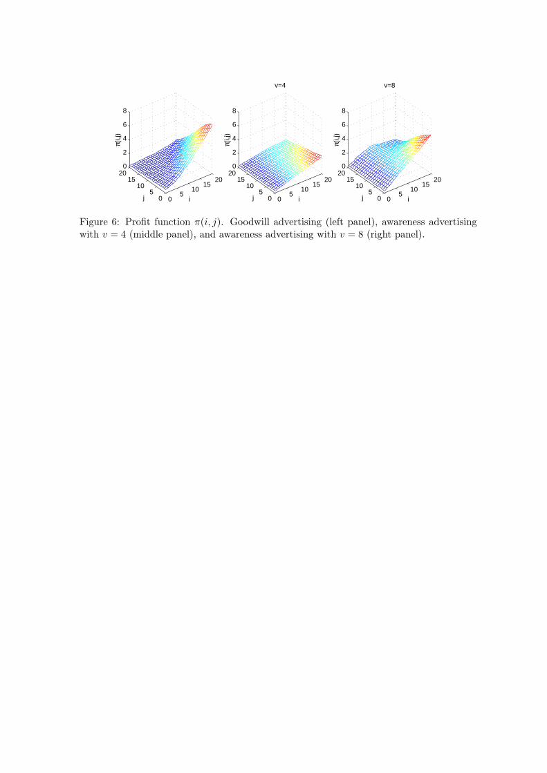
05

1015

20

05

1015

200

2

4

6

8

ij

π(i,j

)

05

1015

20

05

1015

200

2

4

6

8

i

v=4

j

π(i,j

)

05

1015

20

05

1015

200

2

4

6

8

i

v=8

j

π(i,j

)

Figure 6: Profit function π(i, j). Goodwill advertising (left panel), awareness advertisingwith v = 4 (middle panel), and awareness advertising with v = 8 (right panel).

05

1015

20

05

1015

200

2

4

6

8

i

v=4

j

p* (i,j)

05

1015

20

05

1015

200

2

4

6

8

i

v=8

j

p* (i,j)

Figure 7: Equilibrium price p∗(i, j). Awareness advertising with v = 4 (left panel) andv = 8 (right panel).

0 5 10 15 20

0

0.2

0.4

0.6

0.8

1

i

λ(i)

0 5 10 15 200

5

10

15

i

x(i)

0 5 10 15 20

0

0.2

0.4

0.6

0.8

1

i

λ(i)

0 5 10 15 200

5

10

15

20

i

x(i)

Figure 8: Entry deterrence and accommodation. Entry and advertising policy functionsλ(i) and x(i) with entry (solid line) and without entry (dashed). Awareness advertisingwith v = 4 and φe = 375 (top panels) and v = 8 and φe = 675 (bottom panels).

010

20

0

10

200

0.5

1

ij

χ 2(i,j)

010

20

0

10

200

10

20

ij

x 1(i,j)

Figure 9: Exit inducement. Firm 2’s exit policy function χ2(i, j) and firm 1’s advertisingpolicy function x1(i, j). Awareness advertising with v = 8 and φ = 650.