Adverse Selection in Annuity Markets:Evidence from the British Life Annuity Act of

1808

Casey G. Rothschild∗

June 16, 2008

Abstract

We look for evidence of adverse selection using data from an 1808Act of British Parliament which effectively opened up a market for lifeannuities. Our analysis indicates significant selection effects. The evi-dence for adverse selection is particularly strong among a sub-sampleof annuitants whose annuities were purchased by profit-seeking specu-lators. We find evidence of additional selection among self-nominatedannuitants after the annuities were re-priced to reflect the observedlongevity of the early annuitants. The pattern of selection effects isreminiscent of the early stages of an Akerlovian “death spiral,” sug-gesting that adverse selection may be an important factor underlyingthe paucity of annuity sales in contemporary annuity markets. Themagnitudes indicate that it is unlikely to be a complete explanation.JEL N23 D82.

∗ Middlebury College Economics Department, Middlebury, VT 05753. Tel:802.443.5563. Email: crothsch@middlebury.edu. I thank James Poterba,Claudia Goldin, Jerry Hausman, Dora Costa, Peter Temin, Georges Dionne,Norma Coe, Marie-Eve Lachance, Robert Prasch, Raj Chetty (the editor)and two anonymous referees for helpful comments. Any errors are my own.

1 Introduction

In 1808, Britain’s Parliament passed the Life Annuity Act, effectively openinga market for government-provided life annuities. The unique features of theAct provide an unusual opportunity to explore the empirical importance andconsequences of adverse selection.

Adverse selection has played an important role in economic theory sincethe seminal works of Akerlof (1970), Spence (1973), and others. Studyingits empirical importance has proved challenging in several respects. First,as emphasized by Chiappori and Salanie (2000), it is difficult to empiricallydistinguish between moral hazard and adverse selection.

Second, informational asymmetries are likely to extend to researchers,who are unlikely to observe information hidden from the insurance provider.This has motivated the development of tests relying only on ex-ante observ-able information and ex-post outcomes. As described in Dionne et al. (2001),these test for a correlation between insurance choices and ex-post risk, con-ditioning on information observable by the insurance provider. Even thesetests can pose empirical challenges, since econometricians may not even haveaccess to all information symmetrically known by the market participants.

Third, the existing empirical evidence for even the most robust conse-quences of informational asymmetries is less than definitive. For example,Cawley and Phillipson (1999) find no evidence of selection in life insurancemarkets, Cardon and Hendel (2001) find no evidence in health insurancemarkets, and Chiappori and Salanie (2000) and Dionne et al. (2001) find noevidence of adverse selection in auto insurance markets (overturning Pueltzand Snow’s (1994) suggestive evidence). Some economists have recently ar-gued that this absence of evidence may be due to countervailing informationaladvantages of the insurance provider (Villeneuve, 2003) or else to a fourthempirical challenge: the confounding effects of “advantageous” selection viaheterogeneity in risk aversion (DeMeza and Webb, 2001, Cohen and Einav,2007, and Finkelstein and McGarry, 2006).

Annuity markets provide a particularly interesting setting to study infor-mational asymmetries, not least because many of these empirical challengesare less acute than in other insurance settings. In annuity markets, “adverse”selection is expected to lead to a particularly healthy and long-lived annui-tant pool, relative to the population as a whole. This means both that moralhazard is plausibly negligible and that heterogeneity in risk aversion is likelyto be adverse-selection enhancing in annuity markets. Furthermore, annuity

1

providers do minimal risk-classification in practice, so researchers can moreeasily identify characteristics “selected on” by annuitants.

In part for these reasons, annuity markets are one of the few settings inwhich direct evidence of adverse selection has been documented (Finkelsteinand Poterba, 2002, 2004, 2006). Unfortunately, the applicability and gener-ality of this evidence is limited for at least two reasons. First, the evidencecomes from a “compulsory” market, wherein annuitization is mandatory.Second, a substantial literature documents a puzzling dearth of voluntaryannuitization, and understanding this puzzle is crucial for interpreting anyevidence of informational asymmetries in annuity markets.

This paper uses the 1808 Act to provide a novel empirical look at adverseselection in the purely voluntary annuity market effectively opened thereby.We provide evidence of adverse selection by comparing the age- and gender-specific population and annuitant longevities. Since annuity pricing underthis Act varied only by age and gender, our evidence is indicative of selec-tion relative to the risk-classification scheme employed by U.K. government.Insofar as we do not have data on the entire set of information availableto the U.K. government, however, we cannot distinguish perfectly between“selection on observables” (as in Finkelstein and Poterba, 2006) and “pure”adverse selection (as in Dionne et al., 2001).

Beyond documenting adverse selection in a voluntary annuity market,this paper makes two main contributions. First, an odd feature of the 1808Act permitted “speculators” to purchase annuities on the lives of others. InSection 4, we show that the active selection of lives by these speculators wassignificantly stronger than the passive selection by self-nominees.

Second, the Act’s history also provides a unique opportunity to studythe first stages of the type of “death spiral” dynamics found by Cutler andReber (1998) (but not by Buchmueller and DiNardo, 2002) in health insur-ance markets. In Section 5, we show that the pattern of selection effects aresuggestive of the early stages of such a death spiral, but that the magni-tudes indicate these dynamics would not have been sufficient to completelyunravel the market. This is important in light of the extensive literature onthe under-annuitization “puzzle,” since it provides suggestive evidence that,while adverse selection is likely a contributing factor, a “death spiral” is un-likely to fully explain the dearth of annuity sales in contemporary markets.

Before we turn to our main results, Section 2 describes the 1808 LifeAnnuity Act and its subsequent evolution. Section 3 describes the availabledata. Since these data are in an awkwardly condensed form that renders

2

standard survival-curve analysis impossible, Section 3 also a develops a simpleZ-test method for analyzing them; details are contained in a brief technicalappendix. Section 6 concludes.

2 The 1808 Act

Prior to the Life Annuity Act of 1808, British government debt consistedalmost exclusively of Consols – coupon bonds with infinite maturity. Theexplicit goal of the Act was to replace Consols with finite-lived debt by allow-ing the exchange of Consols for life annuities.1 Since Consols were tradableassets, the act effectively opened a life-annuity market.

Annuities sold under this act made twice-annual tax-exempt payments.The size of these payments depended on the interest rate (the market Consolprices) and the age of the annuitant (henceforth: the nominee). Prices weredesigned to be actuarially fair; to that end, they were priced to be 2% moreexpensive than the actuarially fair price implied by the Northampton lifetable. This table, first published by Richard Price in 1771,2 was based onthe mortality experience of all residents of the town of Northampton and wasused widely by life assurance companies (Francis, 1853).

Nominees had to be at least 35 years of age, and annuity yields werecapped at age 75, strongly discouraging purchases by older annuitants. Aminister- or magistrate-certified register of birth or baptism was requiredfor age verification. Verification of non-decease was required for receipt ofeach payment. Finally, the act allowed individuals to purchase and ownthe income stream from annuities on the lives of others (in which case thenominee was required to be from Britain or Ireland).

Shortly after passage of the Act, there appears to have been a recognitionthat the use of the Northampton tables was leading to large government

1There may well have been more subtle motivations leading to its passage. SpencerPerseval, addressing Parliament in 1808 (viz Hendricks, 1856), argued that the Act wouldallow the government to retire debt at favorable interest rates without causing interestrates to rise – an argument Murphy ridicules as indicating Perseval’s desire to “have hiscake and eat it too” (Murphy, 1939, page 6) but which is plausible if the governmentbelieved it could extract surplus by filling a missing market. Alternatively, there couldhave been a political desire to align the interests of the retired monied classes with thegovernment by providing for them a valued service – as argued by Weir (1989) for theFrench government-issued Tontines of the 18th century.

2We transcribed the tables from a republished version in Baily (1813).

3

losses. Murphy (1939) writes that it “was wholly unsuitable as a measure ofthe lower rates of mortality experienced by a self-selected group of annuitants.It was not long before this shortcoming was brought to the attention ofthe Exchequer.” In contrast to Murphy, Francis (1853) suggests that self-selection may have been minor concern relative to active speculation. Hewrites: “The speculators soon found out that the Government charge fora life annuity afforded a very remunerative investment, and the insuranceoffices made considerable profits by purchasing and re-selling them ... Themistake made by Government in its calculations was no secret.”

In 1823, the Parliament finally took active steps to address this per-ceived mispricing and commissioned John Finlaison to study the mortalityexperience of the early nominees.3 His 1829 report developed a new set ofgender-specific life tables, known as the Finlaison tables, based on the ob-served mortality experience of the nominees. After some debate and a briefsuspension of the life annuity program, Parliament determined to resume itwith gender-specific pricing based on these new tables.

This re-pricing made annuities significantly more expensive – especiallyfor females. For example, periodic payments fell by 4.4% and 17% for sixtyyear old males and females, respectively (author’s calculations, based onpricing in Hendriks, 1856). It ironically appears to have coincided with aboom in “speculation,” however, as a result of a contemporaneous decisionto increase the maximum yield to age 90. The old-age mortality experienceunderlying Finlaison’s tables (hence new annuity prices) was primarily thatof young nominees who subsequently grew old. John Francis (1853) relatesa number of amusing anecdotes about speculators realizing that this likelyoverstated the mortality of actively selected older lives and making profitsby combing the countryside for healthy old men to nominate for annuities.4

To address this speculation, an 1834 law reduced the maximum yieldto age 80, and, in practice, eliminated speculative purchases above age 65(Murphy, 1939); speculation was banned outright in 1852 (Cohen, 1953). Themarket for self-nominees continued, with periodic revisions to the life tables,until its dissolution under Parliament’s 1962 Finance Act. Murphy (1939)suggests that these revisions prevented the government from experiencingsignificant losses after 1852 – perhaps in part because private companies

3He also studied nominees of several earlier (and smaller) life-contingent debt issues.4Among these are tales of speculators paying surgeons and clergymen to maintain the

health of the nominees – a rare case of moral hazard in annuity markets.

4

entered the market offering better pricing.5

We exploit three features of this unique history in our study. First, Sec-tion 3 provides evidence of “selection on observables” by documenting a shiftin the gender composition of nominees in favor of men following the adop-tion of gender-specific pricing in 1829. Second, Section 4 provides evidenceof stronger adverse selection effects among speculator-nominated annuitantsvis a vis self-nominees. Third, we use the re-pricing dynamics to test for theearly stages of a “death spiral” in Section 5.

3 Data and Empirical Approach

The only available data are in the highly aggregated form described below.Lacking the individual-level data required for standard survival analysis, wealso briefly discuss our techniques for using them to test for selection effects.

3.1 The Data

Data are available from two reports commissioned by Parliament to examinethe profitability of the annuities sold under the 1808 Act. The first is JohnFinlaison’s 1829 report, which contains data on annuities sold between 1808and 1826. The second is Alexander Glen Finlaison’s 1860 report examiningannuities sold between 1808 and 1850.

John Finlaison’s 1829 report contains one data set for each gender. Eachset consists of three columns of data. The first column is a list of the numberof annuities sold between 1808 and 1826 at each nominee age.6 The secondcolumn gives the number of nominee deaths (between 1808 and January,1826) at each age. The final column reports the distribution of ages, inJanuary 1826, of all “censored” nominees – i.e., those still living in January1826. We do not have individual level observations. Rather, all we observeare three distributions: an aggregate entry age distribution, an aggregatedeath age distribution, and an aggregate age-at-censoring distribution forthe non-censored and censored individuals, respectively.

The 1860 report is in a similar format, but it contains five distinct three-column data classes. The first three describe three distinct classes of “the

5See Hendriks (1856), Murphy (1939), and The Insurance Institute of London (1969)for additional historical details.

6The data refer to the ages of the nominee of a given contract, not the contract’s owner.

5

Table 1: Complete Age 59-64 Speculative Nominee Data SetNumber Number Number Number Number Number

Age Nominated∗ Dead† Living‡ Age Nominated∗ Dead† Living‡

59 7 0 0 68 0 9 3660 50 0 4 69 0 5 4361 61 1 13 70 0 3 4262 91 3 25 71 0 1 2263 81 3 17 72 0 1 464 63 7 17 73 0 0 765 0 8 2 74 0 0 966 0 6 16 75 0 0 467 0 8 34 76 0 0 3

*Between 1828 and 1850. †By May 8, 1854. ‡Nominees still living on May 8, 1854,by age on Dec 31, 1850. Source: A. G. Finlaison (1860).

nominees of those parties who speculated in life annuities” (A. G. Finlaison,1860, p. 14), henceforth speculative nominees, all of whom were males nom-inated after 1828. Each of the three sets appears to represent one or moredistinct investment portfolios put together by a group of speculators. Thefirst contains 353 nominees aged 59 to 64. The second contains 288 nomineesaged 73-84, and the third contains 34 nominees aged 85-92.

The final two data classes in A. G. Finlaison’s report contain informationon all male and female nominees from 1808 to the end of 1850, excluding theaforementioned speculative nominees, but including all nominees in J. Finlai-son’s data. We refer to these nominee classes as “non-speculative,” but it isimportant to note that they may include speculative nominees from the 1808and 1828 period as well as any post-1828 speculator-nominated annuitantsthat the government failed to identify as such.

The first data column in each of the five data classes in the 1860 reportcontains the distribution of the nomination ages in that class. For the non-speculative males and females and the youngest speculative class, the secondcolumn records the death-age distribution for nominees who died between1808 and May 8, 1854. For the two older speculative classes, it instead reportsthe deaths until June 10, 1856. The third column reports the distribution ofages, on December 31, 1850, of all nominees still alive on May 8, 1854 (June10, 1856 for the two older speculative classes).

For illustrative purposes, Table 1 presents the entire data set for theyoungest class of speculative nominees. The rest of the data are in a similarform; we omit them to save space.

6

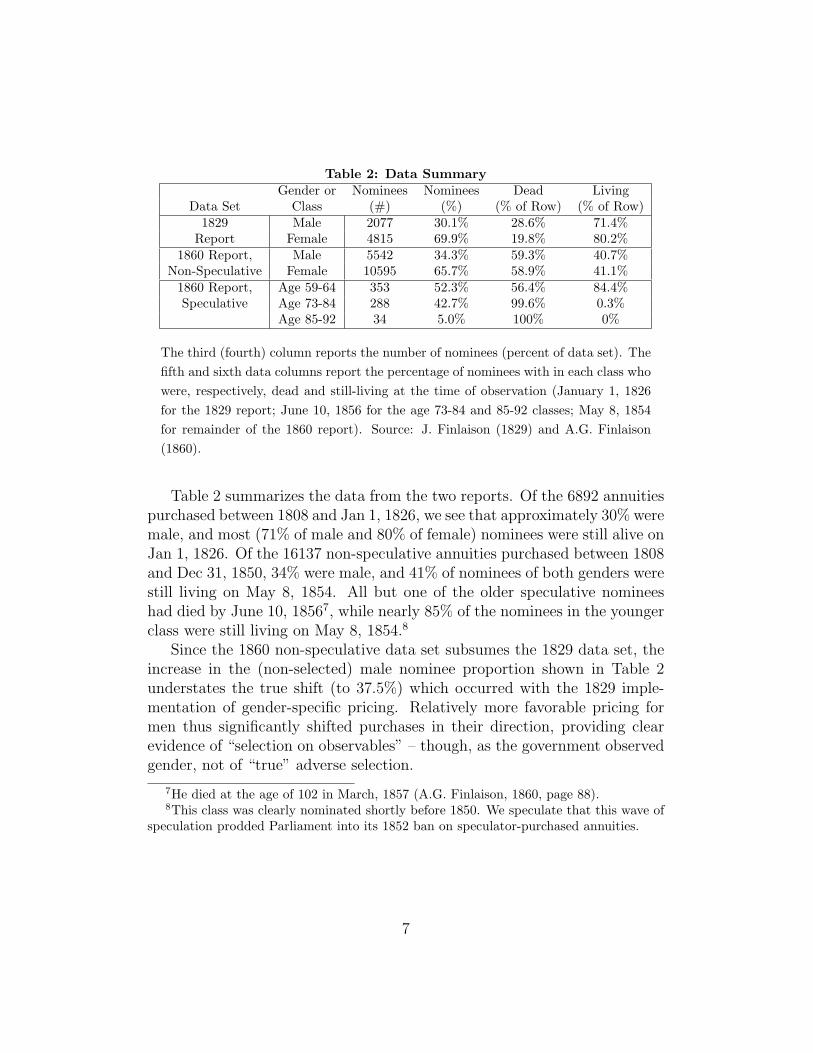
Table 2: Data SummaryGender or Nominees Nominees Dead Living

Data Set Class (#) (%) (% of Row) (% of Row)1829 Male 2077 30.1% 28.6% 71.4%

Report Female 4815 69.9% 19.8% 80.2%1860 Report, Male 5542 34.3% 59.3% 40.7%

Non-Speculative Female 10595 65.7% 58.9% 41.1%1860 Report, Age 59-64 353 52.3% 56.4% 84.4%Speculative Age 73-84 288 42.7% 99.6% 0.3%

Age 85-92 34 5.0% 100% 0%

The third (fourth) column reports the number of nominees (percent of data set). Thefifth and sixth data columns report the percentage of nominees with in each class whowere, respectively, dead and still-living at the time of observation (January 1, 1826for the 1829 report; June 10, 1856 for the age 73-84 and 85-92 classes; May 8, 1854for remainder of the 1860 report). Source: J. Finlaison (1829) and A.G. Finlaison(1860).

Table 2 summarizes the data from the two reports. Of the 6892 annuitiespurchased between 1808 and Jan 1, 1826, we see that approximately 30% weremale, and most (71% of male and 80% of female) nominees were still alive onJan 1, 1826. Of the 16137 non-speculative annuities purchased between 1808and Dec 31, 1850, 34% were male, and 41% of nominees of both genders werestill living on May 8, 1854. All but one of the older speculative nomineeshad died by June 10, 18567, while nearly 85% of the nominees in the youngerclass were still living on May 8, 1854.8

Since the 1860 non-speculative data set subsumes the 1829 data set, theincrease in the (non-selected) male nominee proportion shown in Table 2understates the true shift (to 37.5%) which occurred with the 1829 imple-mentation of gender-specific pricing. Relatively more favorable pricing formen thus significantly shifted purchases in their direction, providing clearevidence of “selection on observables” – though, as the government observedgender, not of “true” adverse selection.

7He died at the age of 102 in March, 1857 (A.G. Finlaison, 1860, page 88).8This class was clearly nominated shortly before 1850. We speculate that this wave of

speculation prodded Parliament into its 1852 ban on speculator-purchased annuities.

7

3.2 Empirical Methodology

To highlight the empirical challenge posed by our data, note that each nom-inee in a given data set implicitly appears twice: his age at nomination isrecorded, and either his death age or his “censored” age is recorded. However,the data do not provide any way for us to connect these two appearances.

Testing for selection involves answering the question: Did the nomineeslive longer than we would have expected? To answer this question with ourdata, we first develop a simple test which applies when we know the deathages of all nominees. We then extend the test to account for censoring.

Take as given a population mortality table −→q = (q0, q1, q2, · · · , q109, q110),where qt denotes the age-t mortality hazard (i.e., the probability of dyingbefore turning t + 1, conditional on having reached age t), and where weassume that nobody survives beyond age 110. View the first column ofdata from each nominee class as a known vector −→e = (e0, e1, · · · , e109, e110),where et is the number of age t nominees. Let d denote the realized valueof the (random) average death age of the nominees. We then test whetherd is significantly greater than we would have expected given −→e and −→q .Specifically, the test statistic:

Z =d− E

[d|−→e ,−→q

]√V[d|−→e ,−→q

] , (1)

has an asymptotic standard normal distribution, where E[d|−→e ,−→q

]and

V[d|−→e ,−→q

]are, respectively, the expected value and the variance of d (given

−→q and −→e ). High Z scores are then evidence of a nominee pool which isadversely selected relative to −→q .

Equation 1 is based on the difference between the expected and actualdeath ages of the nominees. Unfortunately, most of our data sets have “cen-soring:” we do not know actual death ages, and we cannot use Equation1. Instead, we develop an analogous test based on comparing the uncondi-tionally expected death ages of the nominees with the expected death ageconditional on the observed mortality experience up to the time of censoring.

To compute the latter we combine two pieces: the known death ages−−−→dearly of

those who died before censoring (i.e., the second data column), and the ex-pected average death ages of the still-living nominees, computed using their

age distribution−→l (i.e., the third data column)9 and the mortality table −→q .

9For the 1860 data sets, there is a discrepancy between the third column of data and

8

Equation 2 describes a formal test statistic Z ′ based on this intuition. Theappendix establishes that Z ′ has an asymptotic standard normal distribution.

Z ′ =E[d|−→l ,−−−→dearly,−→q ]− E[d|−→e ,−→q ]√

V [d|−→e ,−→q ]− V [d|−→l ,−−−→dearly,−→q ]

(2)

The terms in the numerator of Equation 2 are the conditional and uncondi-tional expected mean death ages described above. The denominator’s termsare conditional variances of the average death age: the first is conditional

only on −→e ; the second is conditional on the realized values of−→l and

−−−→dearly.

Note that the conditionally expected average death age is computed underthe assumption that the “censored” individuals will age according to −→q . Thisreduces the power of the Z ′-test vis-a-vis the simple Z-test: when the actualmortality of the annuitant class being tested differs from −→q , the conditionally

expected average death age E[d|−→l ,−−−→dearly,−→q ] is biased towards E[d|−→e ,−→q ],

particularly in the presence of extensive censoring.Each term in Equation 2 can be directly computed to arbitrary precision

by simulation. We compute E[d|−→e ,−→q ] and V [d|−→e ,−→q ] for a given mortalitytable−→q by simulating 8000 final death profiles for the nominee population−→e .

Similarly, we compute E[d|−→l ,−−−→dearly,−→q ] and V [d|

−→l ,−−−→dearly,−→q ] by simulating

8000 final death profiles−−→dlate for the still-living population

−→l .

3.3 Basic Z-Test Results

We now present raw results based on the Z-tests described in Equations 1and 2. Sections 4 and 5 below detail their implications.

Table 3 uses Equation 2 to test the appropriateness of the Northamptontables for the male and female nominees in the 1829 data set. It indicatesthat the early nominees of both genders are conditionally predicted to livesignificantly longer than unconditionally predicted by the population averagemortality tables, with males and females living an estimated average of .63(i.e., 72.97− 72.34) and 1.53 years longer, respectively. Note again that thisconditional prediction likely understates the degree of adverse selection, asthe conditional prediction is made under the assumption that the survivorswill age according to the Northampton tables.

−→l , since the data report the “censored” age as of December 31, 1850, but the “censoring”

actually occurs later (e.g., May 8, 1854).

9

Table 3: Testing for Adverse Selection,Northampton Tables

E(d) σ Z ′

Unconditional ConditionalMales, 1826 72.34 72.97 0.126 5.02

Females, 1826 71.31 72.84 0.082 18.72

Testing for adverse selection of the early nominees relative to the Northampton table.E(d) refers to the expected average nominee death age of all nominees. Column“Unconditional” (“Conditional”) reports the unconditional expected average deathage (the expected average death age conditional on the observed mortality historythrough 1826). Column σ is the estimated standard error of the difference betweenthese two columns. Z ′ is the Z-score of the difference (viz Equation 2).

Table 4 uses Equations 1 and 2 to test the appropriateness of Finlaison’stables for each of seven classes of nominees.

The final two rows of Table 4 suggest that Finlaison’s life tables were ap-propriate for describing the mortality of the 1808-1826 nominee population:males and females are conditionally and unconditionally predicted to have astatistically (and economically) identical average death ages.

The first two rows of Table 4 indicate that non-speculative 1808-1850male and female nominees are conditionally predicted to live an average of0.84 and 0.22 years longer than would be unconditionally predicted. Bothare statistically significant at standard levels.10

The middle 3 rows of Table 4 indicate that all three classes of speculativenominees lived significantly longer than predicted by the Finlaison tables.11

This is evidence of selection among speculator-selected nominees. Note, how-ever, that we cannot distinguish whether this was true adverse selection orselection on observables: there may have been other symmetrically known

10The pre-1828 nominees are a subset of these nominees. Hence, this is a pure testfor additional selection amongst post-1828 nominees only insofar as the Finlaison tablesaccurately describe the mortality of early nominees. Similarly, these results understatethe degree of adverse selection among the post re-pricing nominees insofar as they involvepooling the un-selected early nominees with the selected later nominees.

11Francis (1853) indicates why speculators selected older nominees. The post 1829pricing was based on the mortality experience of the early nominees, and, since payoutsfrom early annuities were capped at age 75, there were few nominees above this age priorto 1828. Hence, the old-age mortality experience underlying Finlaison’s tables was mostlyfrom individuals who were nominated at a young age and subsequently grew old, and likelyexceeded that of selected older lives. Francis relays anecdotes suggesting that speculatorsunderstood this well (viz Footnote 4).

10

Table 4: Testing for Adverse Selection, Finlaison TablesE(d) σ Z, Z ′

Unconditional ConditionalNS Males, 1850 73.79 74.63 0.126 7.81

NS Females, 1850 76.23 76.45 0.087 2.56S Males, 59-64 74.84 77.72 0.320 9.01S Males, 73-84 83.40 84.72 0.230 5.10S Males, 85+ 89.88 91.62 0.329 5.28Males, 1826 73.87 73.87 0.123 −0.05

Females, 1826 76.12 76.11 0.086 −0.17

Testing with Finlaison’s tables. “NS” and “S” refer to non-speculative and speculativeclasses, respectively. E(d) refers to the expected average death age of all nominees.Column “Unconditional” (“Conditional”) reports the unconditional expected averagedeath age (expected average death age conditional on the observed mortality historythrough 1854, 1856, or 1826 for the first four rows, the fifth row, and the final two rows,respectively). Column σ is the estimated standard error of the difference between thetwo death age estimates. Z,Z ′ is the Z-score of the difference between the conditionaland unconditional averages death ages (viz Equations 1 and 2).

information (e.g., township of birth) that we do not observe.

4 Selection Effects

4.1 Selection Among Early Annuitants

Under the 1808 act, Parliament priced annuities under the assumption thatthe Northampton tables correctly captured the mortality of the British pop-ulation. The results in Table 3 thus indicate at least one of two things: thatthere was significant selection amongst the early nominees, or that Parlia-ment’s assumption about the Northampton table was incorrect.

The Northampton table was based on the mortality history of residentsin a single town, and it was developed from observations in the middle andlate 1700s. So there is clearly reason to view with some skepticism its appro-priateness as a measure of population average mortality in the early 1800s.Unfortunately, reliable data on mortality rates prior to 1838 – when theBritish Government began systematically recording all births and deaths –are lacking (McKeown and Record, 1962). The earliest reliable populationmortality table – known as the English Life Table 3 (ELT3) – was developedby William Farr on data collected between 1838 and 1853 (Farr, 1864). Table

11

Table 5: Comparing Selection Effects Across Life TablesExcess Years Lived (Z-score)

Class Northampton Finlaison ELT3Males, 1826 0.63 (5.0 ) 0.00 (0.0 ) 0.35 (2.9 )Females, 1826 1.53 (18.7 ) -0.01 (-0.2 ) 0.91 (11.6 )NS Males, 1850 2.24 (20.9 ) 0.84 (7.8 ) 2.00 (14.4 )NS Females, 1850 3.90 (46.9 ) 0.22 (2.6 ) 2.51 (30.2 )

This table reports the difference between the conditional and unconditional expectednumber of years lived for three life tables (the Northampton, Finlaison, and EnglishLife Table 3 described in the text) and four nominee classes. Parentheses denoteZ-scores (viz Equation 2).

5 compares the magnitudes of the selection effects relative to the Northamp-ton, Finlaison, and ELT3 tables. It indicates that there were significantselection effects among early nominees relative to ELT3, though the effectsare slightly more modest than those indcated by the Northampton table. TheNorthampton tables may have been inappropriate, but the selection effectsappear to have been important nevertheless.12

4.2 Selection Among Later Annuitants

Regardless of why the early nominees look selected relative to the Northamp-ton tables, the Finlaison tables appear to have done a good job capturingtheir mortality. Table 4 therefore indicates that later nominees were longerlived than Finlaison’s tables predicted. We take this as evidence that theywere more selected than early nominees.

In principle, this apparent additional selection may instead reflect a timetrend in mortality rates. As mentioned above, the lack of reliable data priorto 1838 prevents a definitive resolution of the practical importance of timetrends. Wrigley and Schofield (1981, pages 230 ff), using a sophisticatedback-estimating technique, infer that life expectancy at birth exhibited amild upward trend in the first half of the 19th century. But Greenwood(1936), examining post-1841 data, indicates that this trend was driven byearly-life mortality, stating:

When the historical sequence is examined... [O]ne could hardlysay that the rate at 35-45 had hardly moved decisively before the

12As we discuss below, time trends in mortality could in principle confound this inter-pretation, but seem unlikely to be a problem in practice.

12

Figure 1: Conditional and Unconditional Expected Death Distributions

early eighties, or that at ages 45-55 until the turn of the century.In old age, improvement is now barely perceptible. (page 678)

The age specific mortality trends presented in McKeown and Record (1962)confirm this. This suggests that the increased longevity of the later nomineesrelative to the earlier nominees was largely due to additional selection effectsrather than time trends.

4.3 Comparing the Degrees of Selection

Table 4 indicates that both the speculative and non-speculative nomineesfrom A. G. Finlaison’s data set display higher longevity than the Finlaison(or ELT3) tables predict. We take two approaches to understanding the ex-tent to which the various nominee classes were selected. First, for a visualsense of the degree of selection, Figure 1 plots the conditional and uncondi-tional expected age-at-death distributions according to Finlaison’s tables forthe females and non-speculative males. We see a notable rightward shift ofthe conditional distribution relative to the unconditional distribution, par-ticularly for the males classes.

To quantitatively address the degree of selection, our second approachinvolves computing a “longevity enhancement factor” (LEF) for each nomineeclass. LEF is defined as:

LEF =Actual average death age− Expected average death age

Expected average death age − Average nomination age. (3)

13

Table 6: Estimated Longevity EnhancementsClass Lower Bound LEF Upper Bound LEFNon-Speculative Males, 1850 5.65% 9.06%Non-Speculative Females, 1850 1.17% 1.80%Speculative Males, 59-64 22.56% 121.91%

Exact LEFSpeculative Males, 73-84 25.37%Speculative Males, 85+ 94.02%

Estimated “longevity enhancement factors” (LEF): the percentage by which thelongevity of a given group of nominees exceeded the longevity predicted by Finlaison’smortality tables.

Intuitively, it measures the percent by which average longevity exceeds pre-dicted longevity.

The structure of the data prevents a direct computation of a LEF whenthere is “censoring,” so we instead compute upper and lower bounds on theLEF. Our lower bound assumes that the still-living nominees subsequentlyage according to the Finlaison tables. Our upper bound assumes insteadthat the still-living nominees have equal proportional enhancements priorand subsequent to censoring.13

Table 6 reports our calculations. We see that the longevity of the spec-ulative classes was substantially more enhanced – relative to expectations– than the longevity of the non-speculative classes. The non-selected malesare estimated to have lived between 5.65% and 9.06% longer than the Fin-laison tables predicted. In contrast, the selected groups are estimated to livemore than 20% and as much as 122.91% longer than the Finlaison tablespredicted. The longevity of the non-selected female nominee class appearseven less selected than the males, with a LEF estimated to be between 1.17%and 1.80%.14

13Formally, the upper bound LEF solves:

NT ·(AN+(E[AF ]−AN )(1+LEF )) = ND ·AD+NL·(AL+(E[ALD|~l]−AL)(1+LEF )), (4)

where: NT , ND, and NL are the number of nominees, the number of nominees who haddied by the time of observation, and the number of living nominees, respectively; AN ,AD, and AL are the average ages of the nominees, the dead nominees, and the livingnominees, respectively; and E[AF ] and E[ALD|~l] are the expected average death age ofthe nominees at nomination and the expected (using Finlaison’s tables) average death ageof the censored nominees.

14Note that all the “enhancement” is attributable to the post-1826 nominees; this does

14

The relative enhancement of the non-selected males and the non-selectedfemales may stem from the combination of gender-blind early pricing andthe fact that the pre-1828 data on which the Finlaison tables were based didnot distinguish between “speculative” and “non-speculative” nominees. Themost profitable nominees in the gender neutral pre-1829 pricing regime werethe longer lived females, and Table 4 indicates that speculators were quitegood at selecting long-lived nominees. So Finlaison’s female life tables mayreflect the mortality experience of a particularly selected nominee pool.

5 Annuity Markets and Death Spirals

There is a substantial and growing literature on the so-called “annuity puz-zle,” the observation very few individuals voluntarily choose to annuitize theirretirement assets in spite of the benefits economic theory suggests annuitiesprovide. On the theoretical side, Yaari (1965) showed that full annuitizationshould be optimal under specialized circumstances, and Davidoff et al. (2005)have recently shown that the theoretical prediction of significant annuitiza-tion by optimizing individuals is quite general. But on the empirical sidePoterba et al. (2003), Johnson et al. (2004) and others have documented amarked paucity of life annuity purchases by households in the Health andRetirement Survey. This paucity is corroborated by industry sales data indi-cating a paltry $5.9 billion in immediate annuity sales in in the U.S. in 2006(LIMRA, 2007) and by international evidence (James and Vittas, 2004).

A number of papers have attempted to explain the annuity puzzle. Poten-tial explanations include pre-existing (public or company pension) annuities,unfavorable pricing resulting from adverse selection or administrative load-ing (Mitchell et al., 1999), within-household risk pooling for married couples(Brown and Poterba, 2000), bequest motives (Friedman and Warshawsky,1990), higher returns from alternative assets (Milevsky, 1998), the need forliquidity to cover health shock expenditures (Sinclair and Smetters, 2004),the option value of delaying annuitization (Dushi and Webb, 2004), and be-havioral “framing” effects (Brown et al., 2008). Whether some combinationof these explanations can fully resolve the puzzle remains an open question.

The typical approach in this literature is to posit that households arelife-cycle utility maximizers – typically with constant relative risk aversion,

not affect our qualitative conclusions.

15

additively separable utility functions – and to compute the value such in-dividuals would place on having access to private annuity markets. Brown(2000) provides some empirical support for this approach by showing thatindividuals’ stated intentions to annuitize are indeed correlated with the pre-dictions of such models. Nevertheless, a distinct weakness of this approach isthat quantitative conclusions about “optimal” annuitization rely heavily onfunctional-form utility assumptions. Our empirical methodology helps speakto the importance of adverse selection as a possible resolution to the puzzlewithout making any functional form assumptions.

5.1 The 1808 Act and the Annuity Puzzle

The historical evolution of the 1808 Life Annuity Act closely mimics the firststages of an Akerlovian death spiral. The government initially sold annuitiesat prices consistent with what it believed to be population-average longevity.Table 3 indicates that the resulting annuitant pool had significantly higherlongevity. In 1829, it repriced the annuities based on the mortality of theearly annuitants. Table 4 indicates that the new annuitant pool had signifi-cantly higher longevity than even this new table indicated.

This evidence indicates that the adverse selection spiral was not complete:additional rounds of re-pricing and market thinning were clearly needed.Nevertheless, we are inclined to tentatively interpret the results as at leastmoderately suggestive of the absence of a complete death spiral – at leastfor females. Several factors contribute to this interpretation. First, whilethe non-selected females from A. G. Finlaison’s data set were statisticallysignificantly longer-lived than the Finlaison mortality tables indicated, theabsolute magnitude of the longevity enhancement is modest. This suggeststhat additional re-pricing “rounds” were unlikely to raise prices so dramati-cally as to significantly reduce the population of female annuitants.

Second, the market for annuities did not get markedly thinner in responseto the 1829 re-pricing: Table 2 can be used to show that the annual numberof annuities sold fell by only about 10% after re-pricing.

Third, a back-of-the-envelope calculation suggests that the absolute sizeof the market was substantial. Wrigley and Schofield (1981, page 529) provideBritish population data by broad age category. Of a total 1816 populationof approximately 10 million, we infer that not more than about 25% wereold enough to reasonably consider purchasing an annuity. Only a fraction ofthe resulting 2.5 million potential annuitants would have had the resources

16

to actually buy one: the 1808 act required a minimum of £100 to purchasean annuity (Parliamentary Papers, 1808), and data from Marshall (1833,pages 212 and 214) indicates that the average annuity size between 1817 and1832 was over £1100. Soltow (1968) presents data on the income of variousclasses of the British population between 1801 and 1803. We infer fromSoltow’s data that only 4.3% of the population had annual family incomesin excess of £200. Even if we take this low bound on the income requiredto reasonably consider purchasing annuities, only about 100,000 individualswere plausible candidates for annuities. The 16,000 annuities sold underthe 1808 act between 1808 and 1850 thus represents a substantial fractionof a plausible upper bound on the total number sold. (Taking the annualincome cutoff to equal the average annuity size makes the results even starker,reducing the plausible candidates to about 7500 individuals.)15

These considerations together suggest that there was scope for a well-functioning “thick” market for non-speculative life annuities – at least forfemales. Though one must be cautious about extrapolating to contemporarymarkets, this at least provides some suggestive evidence that a “death spiral”driven by standard self-selection is unlikely to explain the annuity puzzle.

6 Discussion and Conclusions

The United Kingdom’s 1808 Life Annuity Act effectively opened up a marketfor government-provided life annuities. Analysis of data on purchases andsubsequent mortality rates suggests that the market was characterized by twotypes of adverse selection: classic “self-selection” whereby individuals pur-chasing annuities for themselves were healthier than the average individualin the population, and “speculative” selection, whereby pecuniary-mindedindividuals or institutions took advantage of an odd feature of the act whichallowed them to purchase annuities contingent on the lives of others.

Our results indicate that self-selection of annuitants was substantial: theannuitant pool between 1808 and 1826 appears to have been dramatically

15Additionally, though we have had not had luck finding data from after 1850, Murphy(1936) indicates that the market continued to exist and stabilize after speculation wasbanned in 1852. One must interpret this cautiously, however: by the late 1800s, theconfounding effects of improving mortality trends begin to bite. Furthermore, Murphyreports that the market was fairly modest in size by the early 1900s, in part because therewere better-priced private-sector annuity options by this time.

17

longer lived than the population as a whole, even when we account for theage and gender of the annuitants. Furthermore, a 1829 attempt by thegovernment to re-price annuities to reflect the higher longevity of the earlyannuitants resulted in an annuitant pool that was longer lived still. Thisis reminiscent of the early stages of a death spiral, though the degree towhich the later annuitants were selected and the robustness of the marketsize suggests that, while adverse selection was clearly an important concern,it is unlikely to have eviscerated the market. This finding reinforces theview that an adverse selection death spiral is unlikely to explain the puzzlingdearth of annuity sales in contemporary markets.

Our analysis also indicates that speculators effectively selected particu-larly long-lived individuals to nominate for annuities and profited consid-erably at the expense of the government from the Act. This recommendscare to modern policy makers when contemplating expanding choice in gov-ernment provided services: when choices can be made by pecuniary-mindedindividuals or institutions, selection effects may be significantly exacerbatedand may impose particularly large costs on the government.

References

[1] George Akerlof. The market for ‘lemons’: Quality uncertainty and themarket mechanism. Quarterly Journal of Economics, 84(3):488–500,1970.

[2] Francis Baily. The Doctrine of Life-Annuities and Assurances. JohnRichardson, London, 1813.

[3] Jeffrey Brown. Private pensions, mortality risk, and the decision toannuitize. Journal of Public Economics, 82:29–62, 2001.

[4] Jeffrey Brown, Jeffrey Kling, Sndhil Mullainathan, and Marian Wrobel.What don’t the people insure late life consumption? a framing expla-nation of the under-anuitization puzzle. American Economic ReviewPapers and Proceedings, 98(2), 2008.

[5] Jeffrey Brown and James Poterba. Joint life annuities and the annuitydemand by married couples. Journal of Risk and Insurance, 67(4):527–553, 2000.

18

[6] Thomas Buchmueller and John DiNardo. Did community rating inducean adverse selection death spiral? evidence from new york, pennsylvania,and connecticut. American Economic Review, 92:280–294, 2002.

[7] James Cardon and Igal Hendel. Asymmetric information in health in-surance: evidence from the national medical expenditure survey. RANDJournal of Economics, 32:408–427, 2001.

[8] John Cawley and Tomas Philipson. An empirical examination of in-formation barriers to trade in insurance. American Economic Review,89:827–846, 1999.

[9] Pierre-Andre Chiappori and Bernard Salanie. Testing for adverse se-lection in insurance markets. Journal of Political Economy, 108:56–78,2000.

[10] Alma Cohen and Liran Einav. Estimating risk preferences from de-ductible choice. American Economic Review, 97, 2007.

[11] Jacob Cohen. The elements of lottery in british government bonds,1694-1919. Economica, 20, 1968.

[12] David Cutler and Sarah Reber. Paying for health insurance: The trade-off between competition and adverse selection. Quarterly Journal ofEconomics, 113:433–466, 1998.

[13] Thomas Davidoff, Jeffrey Brown, and Peter Diamond. Annuities andindividual welfare. American Economic Review, 95:1573–1590, 2005.

[14] David de Meza and David Webb. Advantegeous selection in insurancemarkets. The RAND Journal of Economics, 32:249–262, 2001.

[15] Georges Dionne, Christian Gourieroux, and Charles Vanasse. Testingfor evidence of adverse selection in the automobile insurance market: Acomment. Journal of Political Economy, 109:444–453, 2001.

[16] Irene Dushi and Anthony Webb. Household annuitization decisions:Simulations and empirical analyses. Journal of Pension Economics andFinance, 3:109–143, 2004.

19

[17] William Farr. English Life Tables: Tables of Lifetimes, Annuities andPremiums. Longman, Green, Longman, Roberts and Green, London,1864.

[18] Amy Finkelstein and James Poterba. Selection effects in the market forindividual annuities: New evidence from the United Kingdom. EconomicJournal, 112:28, 2002.

[19] Amy Finkelstein and James Poterba. Adverse selection in insurancemarkets: Policyholder evidence from the U.K. annuity market. Journalof Political Economy, 112:183–208, 2004.

[20] Amy Finkelstein and James Poterba. Testing for adverse selection with‘unused observables’. NBER Working Papers, 12112, 2006.

[21] Amy Finkelsten and Kathleen McGarry. Multiple dimensions of pri-vate information: Evidence from the long-term care insurance market.American Economic Review, 96:938–958, 2006.

[22] Alexander Glenn Finlaison. Tontines and life annuities. Republishedin Rates of Mortality, B. Benjamin, ed., Gregg International PublishersLTtd., Germany 1973, 1860.

[23] John Finlaison. Report of John Finlaison. House of Commons Parlia-mentary Papers, March 31, 1829.

[24] John Francis. Annals, Anecdotes and Legends: A Chronicle of LifeAssurance. Longman, Brown, Green and Longmans, London, 1853.

[25] Benjamin Friedman and Mark Warshawsky. The cost of annuities: Im-plications for savings behavior and bequests. Quarterly Journal of Eco-nomics, 105:135–154, 1990.

[26] Major Greenwood. English death rates, past, present and future: Avaledictory address. Journal of the Royal Statistical Society, 99(4):674–707, 1936.

[27] Frederick Hendriks. On the financial statistics of British governmentlife annuities (1808-1855), and on the loss sustained by government ingranting annuities. Journal of the Statistical Society of London, pages325–384, 1856.

20

[28] LIMRA International. U.S. individual annuities. 1, 2007.

[29] Estelle James and Dimitri Vittas. Annuity markets in comparative per-spective: Do consumers get their money’s worth? World Bank Devel-opment Reseach Group, 2004.

[30] Richard Johnson, Leonard Burman, and Deborah Kobes. Annuitizedwealth at older ages: Evidence from the health and retirement survey.Urban Institute, 2004.

[31] John Marshall. Digest of 600 volumes of journals, reports, and papers,preseneted to parliament since 1799. Goldsmith-Kress Collection (Har-vard business school), 27862.

[32] Thomas McKeown and R. G. Record. Reasons for the decline of mor-tality in england and wales during the nineteenth century. PopulationStudies, 16(2):94–122, 1962.

[33] Moshe Milevsky. Optimal asset allocation towards the end of the lifecycle: To annuitize or not to annuitize? Journal of Risk and Insurance,65:401–426, 1998.

[34] Olivia S. Mitchell, James M. Poterba, Mark Warshawski, and JeffreyBrown. New evidence on the moneys worth of individual annuities.American Economic Review, 89(5):1299–1318, 1999.

[35] Ray D. Murphy. Sale of annuities by governments. In Address at theThirty-Third Annual Convenction of The Association of Life InsurancePresidents, 1939.

[36] The Insurance Institute of London. The history of individual annuitycontracts, 1969.

[37] Parliamentary Papers. Life annuities: Abstract and explanation of theact for enabling the commissioners for the reduction of the national debtto grant life annuities by the transfer of funded property. Hansard andSons, 1808.

[38] James Poterba, Joshua Rauh, Steven Venti, and David Wise. Utilityevaluation of risk in retirement savings accounts. NBER Working Pa-pers, 9892, 2003.

21

[39] Richard Price. Observations on Reversionary Payments, 7ed. Cadwelland Davies, London, 1812.

[40] Robert Puelz and Arthur Snow. Evidence on adverse selection: Equilib-rium signalling and cross subsidization in the insurance market. Journalof Political Economy, 102:236–257, 1994.

[41] Sven Sinclair and Kent Smetters. Health shocks and the demand forannuities. Congressional Budget Office Technical Papers Series, 2004.

[42] Lee Soltow. Long-run changes in british income inequality. The Eco-nomic History Review, New Series Vol. 21(1), 1968.

[43] Michael Spence. Job market signaling. Quarterly Journal of Economics,87(3):355–374, 1973.

[44] Bertrand Villeneuve. Competition between insurers with superior infor-mation. European Economic Review, 49:321–340, 2003.

[45] David Weir. Tontines, public finance, and revolution in France andEngland, 1688-1789. Journal of Economic History, 49:95–124, 1989.

[46] E. A. Wrigley and R. S. Schofield. The Population History of England,1541-1871: A reconstruction. Harvard University Press, 1981.

[47] Menachem Yaari. Uncertain lifetimes, life insurance, and the theory ofthe consumer. Review of Economic Studies, 32:137–150, 1965.

7 Appendix

This appendix shows that the test statistic Z ′, defined in Equation (2), is asymptoticallydistributed as a standard normal random variable.

Fixing a class of nominees (e.g., pre 1829 males), view the random process underlyingthe data as a three-step compound process: (i) process α draws an independent randomage and nomination year for each nominees j = 1, · · · , N from some fixed distribution;(ii) process β draws an independent random lifetime up to the censoring date for j (usingmortality table −→q ); and (iii) random process γ draws an independent random lifetimebeyond the censoring time for censored individuals.

Let mj denote the (random) death age of j, and let bj = Eγ [mj |αj , βj ], which is arandom function of αj and βj . Then:

E[d|−−−→dearly,

−→l ] =

1N

N∑j=1

bj . (5)

22

Since {bj}Nj=1 is a set of i.i.d. random variables, the Central Limit Theorem establishesthat

Z ′ ≡ E(d|−−−→dearly,

−→l )/√V [bj ]/N (6)

has an asymptotic standard normal distribution.Towards deriving the variance of bj , we use the law of iterated expectations:

V [m|α]=Eβ,γ[m2|α

]− (Eβ,γ [m|α])2

=Eβ[V [m|α, β] + (Eγ [m|α, β])2

]− (Eβ [Eγ [m|α, β]])2

=Eβ [V [m|α, β]] + Eβ[b2]− (Eβ [b])2

=Eβ [V [m|α, β]] + V [b],

(7)

where we have dropped j subscripts for notational convenience. The α-conditional varianceis thus the sum of two components: the expectation of the β-conditional variance of themean death age plus the variance of the β-conditional expected mean death age.

Re-arranging Equation 7 gives

V [b]/N = V [m|α]/N − Eβ [V [m|α, β]] /N. (8)

To complete our derivation, observe that since the distribution of entrants acrossages −→e /N converges in probability, V [m|α]/N is consistently estimated by the vari-ance of d conditional on the observed entrant distribution, i.e., by V [d|−→e ,−→q ]. Similarly,

Eβ [V [m|α, β]] /N is consistently estimated by V [d|−→l ,−−−→dearly,−→q ]. Equation 2 follows di-

rectly from these observations and Equations 6 and 8.

23