Advances in type-2 fuzzy sets and systems - AMiner · interval type-2 fuzzy sets and systems are...

Information Sciences 177 (2007) 84–110

www.elsevier.com/locate/ins

Advances in type-2 fuzzy sets and systems

Jerry M. Mendel *

Signal and Image Processing Institute, Department of Electrical Engineering, University of Southern California,

3740 McClintock Avenue, Los Angeles, CA 90089-2564, United States

Received 10 January 2006; received in revised form 30 April 2006; accepted 7 May 2006

Abstract

In this state-of-the-art paper, important advances that have been made during the past five years for both general andinterval type-2 fuzzy sets and systems are described. Interest in type-2 subjects is worldwide and touches on a broad rangeof applications and many interesting theoretical topics. The main focus of this paper is on the theoretical topics, withdescriptions of what they are, what has been accomplished, and what remains to be done.� 2006 Elsevier Inc. All rights reserved.

Keywords: Type-2 fuzzy sets; Type-2 fuzzy systems; Interval type-2 fuzzy sets; Interval type-2 fuzzy logic systems; Centroid; KM algo-rithms; Computing with words; Fuzzy weighted average

1. Introduction

Type-2 fuzzy sets (T2 FS), which were introduced by Zadeh in [98], are now very well established and (asshall be demonstrated in this paper) are gaining more and more in popularity. In [51] we find answers to thefollowing:

1. Why did it take so long for the concept of a T2 FS to emerge? It seems that science moves in progressive wayswhere one theory is eventually replaced or supplemented by another, and then another. In school we learnabout determinism before randomness. Learning about type-1 (T1) FSs before T2 FSs fits a similar learningmodel. So, from this point of view it was very natural for fuzzyites to develop T1 FSs as far as possible.Only by doing so was it really possible later to see the shortcomings of such FSs when one tries to use themto model words or to apply them to situations where uncertainties abound.

2. Why didn’t T2 FSs immediately become popular? Although Zadeh introduced T2 FSs in 1975, very little waspublished about them until the mid-to late nineties. Until then they were studied by only a relatively smallnumber of people, including: [13,14,19,20,63,64,66,86]. Recall that in the 1970s people were first learning

0020-0255/$ - see front matter � 2006 Elsevier Inc. All rights reserved.

doi:10.1016/j.ins.2006.05.003

* Tel.: +1 213 740 4445; fax: +1 213 740 4651.E-mail address: [email protected]

mailto:[email protected]

J.M. Mendel / Information Sciences 177 (2007) 84–110 85

what to do with T1 FSs, e.g. fuzzy logic control. Bypassing those experiences would have been unnatural.Once it was clear what could be done with T1 FSs, it was only natural for people to then look at more chal-lenging problems. This is where we are today.

3. Why do we believe that by using T2 FSs we will outperform the use of T1 FSs? T2 FSs are described by mem-bership functions (MFs) that are characterized by more parameters than are MFs for T1 FSs. Hence, T2FSs provide us with more design degrees of freedom; so using T2 FSs has the potential to outperform usingT1 FSs, especially when we are in uncertain environments. Note that, at present, there is no theory that

guarantees that a T2 FS will always do this.

One sign of a vibrant field is its applications. Here we categorize the applications that have appeared in theliterature for T2 fuzzy sets and systems since 2001. For applications prior to that year, see [47, pp. 13–14].

Approximation: [61] (TSK/steel strip temperature); Clustering: [26] (C spherical shells algorithm), [72](fuzzy C-means); Control: [40] (marine and traction diesel engines), [75] (integrated development plat-form), [4] (evolutionary computing/NL dynamic plants), [36] (buck DC–DC converters), [17] (trackingmobile objects/robotic soccer games), [93] (liquid-level), [81] (proportional control), [25] (autonomousmobile robots), [24] (autonomous mobile robots/hierarchical), [44] (adaptive control of nonlinearplants); Databases: [67] (summarization); Decision making: [70] (variation in human decision making);Embedded agents: [10,11] (ambient intelligent environments); Health care: [27] (clinical diagnosis), [9](differential diagnosis), [92] (nursing assessment); Hidden Markov models: [103] (phoneme recognition);Neural networks: [73] (fuzzy perceptron); Noise cancellation: [3] (adaptive noise cancellation); Pattern

classification: [74] (fuzzy k-nearest neighbor); Quality Control: [45] (sound speakers); Spatial query:

[71] (spatial objects); Wireless communications: [35] (wireless sensors/power on-off control), [77] (wirelesssensor network lifetime analysis).

This paper focuses on advances in T2 fuzzy sets and systems since the year 2001, because earlier works arealready well documented, e.g. [47]. The focus is on theoretical and computational issues. While some issueshave been resolved, many new ones have been exposed, so T2 is a very fertile field for research.

Up until 2001, there was a very heavy emphasis on interval T2 FSs (IT2 FSs) and FLSs (IT2 FLSs), pri-marily because of their computational tractability. This emphasis has continued; however, interests have alsoturned towards more general kinds of T2 FSs and systems. Both T2 paths are covered in this paper. Section 2covers topics about general T2 FSs and FLSs, and Section 3 covers topics about IT2 FSs and IT2 FLSs. Sec-tion 4 covers the fuzzy weighted average; Section 5 covers computing with words; and, Section 6 provides ourconclusions.

It is assumed that the reader has some familiarity with T2 fuzzy sets and systems. For a relatively simpleintroduction to the former, see [54], and for the latter, see [47,55].

2. General T2 FSs and FLSs

In Section 2.1 we begin by presenting a Representation Theorem for a T2 FS. It is one of the most usefulresults in T2 FS theory because it can be used to derive many things that are associated with that theory, bothold and new, in a simple and straightforward manner. Unfortunately, is not useful for computation; hence, thelatter needs to be approached from other viewpoints. As for T1 FSs, the fundamental computations for T2FSs are union, intersection and complement, and how to compute them, as well as attendant difficulties insuch computations, are discussed in Section 2.2. One of the major applications for T2 FSs is a rule-basedFLS, namely a T2 FLS, which is overviewed in Section 2.3. The major new calculation in a T2 FLS is calledtype-reduction; it maps a T2 FS into a T1 Fs, after which it is a simple matter to defuzzify the T1 FS in order toobtain a number at the output of the T2 FLS. Type-reduction, which is a major bottleneck for a T2 FLS, isoverviewed in Section 2.4, and new ways for computing it are mentioned.

Zadeh [99–101] has introduced the computing with words (CWW) paradigm. Because words mean differentthings to different people, Mendel [50,51] has argued that words must be modeled using T2 FSs when com-puters interact with people and the interactions use FSs. In order to map from T2 FS word models back intoa word, one will need the concept of similarity of T2 FSs, which is discussed in Section 2.5.

86 J.M. Mendel / Information Sciences 177 (2007) 84–110

2.1. Representation theorem for a T2 FS

Mendel and John [54] have presented the following new representation for a T2 FS.

Theorem 1 (Representation theorem). Assume that primary variable x is sampled at N values,

x1, x2, . . . ,xN, and at each of these values its primary memberships ui are sampled at Mi values,

ui1; ui2; . . . ; uiMi . Let eAje denote the jth T2 embedded set1 for T2 FS eA, i.e.,

1 An2 No

eAje � fðxi; ðuj

i ; fxiðujiÞÞÞ; uj

i 2 fuik; k ¼ 1; . . . ;Mig; i ¼ 1; . . . ;Ng ð1Þ
in which fxiðu
jiÞ is the secondary grade at uj

i . Note that eAje can also be expressed as

eAje ¼

XN

i¼1

½fxiðujiÞ=uj

i �=xi; uji 2 fuik; k ¼ 1; . . . ;Mig ð2Þ

Then eA can be represented as the union of its T2 embedded sets, i.e.,

eA ¼XnA

j¼1

eAje ð3Þ

nA ¼YNi¼1

Mi ð4Þ

This representation of a T2 FS, in terms of much simpler T2 FSs, the embedded T2 FSs, is very useful forderiving theoretical results, as we explain later in this paper; however, it is not recommended for computa-tional purposes, because it would require the explicit enumeration of the nA embedded T2 FSs and nA canbe astronomical.

2.2. Operations on general T2 FSs

Consider two T2 FSs sets2 eA and eB, i.e.,

eA ¼ ZX

l~AðxÞ=x ¼Z

X

ZJu

x

fxðuÞ=u

" #=x; J u

x ¼ fðx; uÞ : u 2 ½l~AðxÞ; �l~AðxÞ�g � ½0; 1� ð5Þ

and

eB ¼ ZX

l~BðxÞ=x ¼Z

X

ZJw

x

gxðwÞ=w

" #=x; J w

x ¼ fðx;wÞ : w 2 ½l~BðxÞ; �l~BðxÞ�g � ½0; 1� ð6Þ

It is well-known [63] that the union of eA and eB is another T2 FS whose MF can be computed from:

l~A[~BðxÞ ¼Z

u2J ux

Zw2Jw

x

fxðuÞHgxðwÞ=ðu _ wÞ ¼ l~AðxÞ t l~BðxÞ; x 2 X ð7Þ

where t denotes the join operation. The use of the notation l~AðxÞ t l~BðxÞ to indicate the join between the sec-ondary MFs l~AðxÞ and l~BðxÞ is, of course, a shorthand notation for the operations in the middle of (7). What (7)says is that to perform the join between two secondary MFs, l~AðxÞ and l~BðxÞ, v = u _ w must be performedbetween every possible pair of primary memberships u and w, such that u 2 J u

x and w 2 J wx and that the sec-

ondary grade of l~A[~BðxÞ must be computed as the t-norm operation between the corresponding secondarygrades of l~AðxÞ and l~BðxÞ, fx(u) and gx(w), respectively. Note that at each value of x the join involves T1FSs (i.e., secondary MFs), and that the join must be computed for "x 2 X. If more than one combination

embedded T2 FS is a T2 FS that has only one primary membership at each xi. It is also called a wavy slice [54].te that (5) means eA : X ! f½a; b� : 0 6 a 6 b 6 1g.


of u and w gives the same point u _ w, then in the join we keep the one with the largest membership grade.Usually, the maximum t-conorm is used, as suggested in [98,63].

In general, evaluating the join is difficult to do for arbitrary T2 FSs. Karnik and Mendel [28] have shownthat for n convex and normal T1 FSs, F1, . . . ,Fn, characterized by MFs f1(h), . . . , fn(h), respectively, wheref1(v1) = � � � = fn(vn) = 1, and the fi(h) are re-ordered so that v1 6 v2 6 � � � 6 vn, the MF of tn

i¼1F i, using max-imum t-conorm and either minimum or product t-norm, can be expressed as

ltni¼1

F iðhÞ ¼

T ni¼1fiðhÞ h < v1

T ki¼1fiðhÞ vk 6 h 6 vkþ1

_ni¼1fiðhÞ h > vn

8><>: 1 6 k 6 n� 1 ð8Þ

Unfortunately, this formula is not so easy to use. Coupland and John [7] have taken a very new and novelapproach to computing the join. Because their approach is also used for computing the meet, we describeit later in this section.

It is also well known [63] that the intersection of eA and eB is another T2 FS whose MF can be computedfrom:

l~A\~BðxÞ ¼Z

u2Jux

Zw2Jw

x

fxðuÞHgxðwÞ=u ^ w ¼ l~AðxÞ u l~BðxÞ; x 2 X ð9Þ

where u denotes the meet operation. The use of the notation l~AðxÞ u l~BðxÞ to indicate the meet between thesecondary MFs l~AðxÞ and l~BðxÞ is another shorthand notation, but this time for the operations in the middleof (9). What (9) says is that to perform the meet between two secondary MFs, l~AðxÞ and l~BðxÞ, v = u ^ w mustbe performed between every possible pair of primary memberships u and w, such that u 2 J u

x and w 2 J wx , and

the secondary grade of l~A\~BðxÞ must be computed as the t-norm operation between the corresponding second-ary grades of l~AðxÞ and l~BðxÞ, fx(u) and gx(w), respectively. This must be done for "x 2 X. If more than onecombination of u and w gives the same point u ^ w, then in the meet (just as in the join) we keep the one withthe largest membership grade.

Note that in (9) there are two t-norms, w and ^. Although they are usually chosen to be the same, they donot have to be. See [78] for very interesting discussions about this.

In general, evaluating the meet is also difficult to do for arbitrary T2 FSs, especially when the product t-norm is used. Karnik and Mendel [28] have also shown that for n convex and normal T1 FSs, F1, . . . ,Fn, char-acterized by MFs f1(h), . . . , fn(h), respectively, where f1(v1) = � � � = fn(vn) = 1, and the fi(h) are re-ordered sothat v1 6 v2 6 � � � 6 vn, the MF of un

i¼1F i using maximum t-conorm and minimum t-norm can be expressed as

luni¼1

F iðhÞ ¼

_ni¼1fiðhÞ h < v1

^ki¼1fiðhÞ vk 6 h 6 vkþ1 1 6 k 6 n� 1

^ni¼1fiðhÞ h > vn

8><>: ð10Þ

Unfortunately, it is still difficult to use (10). To-date, no formula that is similar to (10) exits for the product t-norm, which is unfortunate because many applications use product t-norm. When all MFs are Gaussian, thenKarnik and Mendel [28] have an approximation for computing the meet under product t-norm, one that leadsto another Gausssian MF, so that the approximate meet is ‘‘reproducing’’, and can be expanded in multi-argu-ment form.

The usual derivations of (7) and (9) utilize Zadeh’s extension principle. Mendel and John [54] show how (7)and (9) can easily be derived without having to use the extension principle, when eA and eB are represented as inTheorem 1. These derivations were the first theoretical uses of the new Representation Theorem.

Coupland and John [6,7] have shown how to compute the join and meet of eA and eB using methods fromcomputational geometry (e.g., a modified Weiler–Atherton clipping algorithm, and a Bentley–Ottman planesweep algorithm). Their approach is based on modeling a secondary MF geometrically as a [7] ‘‘set of con-nected straight line segments that need not be equally-spaced across the domain’’, and is limited so far tothe minimum t-norm and the maximum t-conorm. They distinguish between a partially discrete T2 FS anda discrete T2 FS. A partially discrete T2 FS is one whose primary variable is discrete (sampled) but whose sec-ondary MFs are continuous, whereas a discrete T2 FS is one whose primary variable and secondary MFs are


discrete (sampled). Based on extensive simulations of a two-rule FLS in which each rule has two-antecedents,and the secondary MFs are discretized into 10 points, and are also described by two line segments, Couplandand John obtain over a ‘‘four and a half fold increase in inferencing speed’’. They also state ‘‘. . . that for anyT2 FLS with secondary MFs with five or more discretizations, using a partially discrete model would give afaster and more accurate system’’. This approach to computing operations for general T2 FSs looks verypromising and is continuing.

When secondary MFs are triangular (an interesting compromise between interval secondary MFs and gen-eral secondary MFs, and one that is also considered by Coupland and John [7]) then Starczewski [78,79] hasshown that ‘‘extended t-norms3 of triangular fuzzy truth values may be approximated by triangular fuzzytruth values as well’’. One of the most interesting aspects of Starczewski’s [79] approach is it ‘‘. . . reduces cal-culations of extended t-norms (a similar approach can be rearranged for s-norms) to computing only the threecharacteristic functions: principal, upper and lower. Arbitrary traditional t-norms (or s-norms) can be used tocalculate these functions. A tremendously useful feature of this approach is that the resultant MF preservestriangular shapes of the two arguments, and this way the approximate t-norms can be expanded to multi-argu-ment form. Moreover, for each triangular fuzzy membership grade only three parameters have to be storedand processed by [a] FLS, instead of tabularized functions as in the general approach’’. Another very usefulfeature of this approach is that formulas are given for the operations, so that explicit derivative formulas canbe obtained if a triangular T2 FLS is designed (optimized) using a method that requires such derivatives (e.g.,steepest descent). Starczewski’s results also seem very promising and are continuing. Some additional work byhim for Gaussian T2 FSs is in [80].

In a (singleton) T2 FLS the meet may only have to be computed at a single value of x, namely x = x 0.

Definition. In general,

3 AnTanak

4 Th

eA ¼ fððx; uÞ; l~Aðx; uÞÞj8x 2 X ; 8u 2 J x � ½0; 1�g ð11Þ
in which l~Aðx; uÞ is the T2 MF of eA. By a type-2 fuzzy singleton, we mean a T2 FS for which
l~Aðx; uÞ ¼1=1 x ¼ x0

1=0 8x 6¼ x0

�ð12Þ

In (12), 1/1 (1/0) means that at x = x 0, when its primary variable u = 1 (u = 0), the associated secondary gradeequals 1. At all other values of u the secondary grade equals 0; hence, by convention, such secondary gradesare not shown.

Example. The meet between a T2 singleton, eA, and a normal4 T2 FS, eB, under minimum and product t-normsis a widely used operation in a T2 FLS (Section 2.3), and is (for a derivation, see [47, p. 222]):

l~AðxÞ u l~BðxÞ ¼l~Bðx0Þ x ¼ x0

1=0 8x 6¼ x0

�ð13Þ

Observe that the meet between a type-2 singleton, eA, and a T2 FS, eB, sifts out a specific vertical slice ofl~Bðx; uÞ, namely l~Bðx0Þ, the secondary MF at x = x 0.

Because it is very easy to compute the complement of eA, we do not discuss it here.Finally, Walker and Walker [87–89] have many interesting and important mathematical results about join

and meet within the framework of the algebra of truth values of T2 FSs. How these results can be applied isworth exploring.

extended t-norm is a t-norm obtained by applying the Extension Principle to a T1 t-norm. It was the basis for Mizumoto anda’s [63] works.is means the secondary MFs of eB reach the value 1.

Type-2 FLS

Type-reducedSet (Type-1)

Rules Defuzzifier

Crisp

inputs

Fuzzy

input sets

Fuzzy

output sets

Crisp

outputy

x

Fuzzifier

Inference

Type-reducer

Output Processing

Fig. 1. Type-2 FLS.


2.3. Type-2 FLS

A general T2 FLS is depicted in Fig. 1. It is very similar to a T1 FLS, the major structural difference beingthat the defuzzifier block of a T1 FLS is replaced by the output processing block in a T2 FLS. That block con-sists of type-reduction (TR) followed by defuzzification. We will have a lot to say about TR in Sections 2.4 and3.5.

Consider a T2 FLS having p inputs x1 2 X1, . . . ,xp 2 Xp, one output y 2 Y, and M rules, where the lth rulehas the form

5 De

Rl : IF x1is eF l1 and � � � and xp is eF l

p; THEN y is eGl l ¼ 1; . . . ;M ð14Þ

This rule represents a T2 relation between the input space X1 · � � � · Xp, and the output space, Y, of the T2FLS. Each rule in (14) is interpreted as a T2 fuzzy implication. With reference to (14), leteF l

1 � � � � � eF lp ¼ eAl; then, as is well known, (14) can be re-expressed as

Rl : eF l1 � � � � � eF l

p ! eGl ¼ eAl ! eGl; l ¼ 1; . . . ;M ð15Þ

Rl is described by the MF lRlðx; yÞ ¼ lRlðx1; . . . ; xp; yÞ, where5

lRlðx; yÞ ¼ l~Al!~Glðx; yÞ ¼ ½upi¼1l~F l

iðxiÞ� u l~GlðyÞ ð16Þ

Most generally, the p-dimensional input to Rl is given by the T2 FS eAx whose MF is

l~AxðxÞ ¼ up

i¼1l~X iðxiÞ ð17Þ

where ~X i ði ¼ 1; . . . ; pÞ are the labels of the FSs describing the inputs. Each rule Rl determines a T2 FSeBl ¼ eAx � Rl such that

l~BlðyÞ ¼ l~Ax�RlðyÞ ¼ tx2X½l~AxðxÞ u lRlðx; yÞ�; 8y 2 Y l ¼ 1; . . . ;M ð18Þ

This equation is the input–output relation in Fig. 1 between the T2 FS that excites one rule in the inferenceengine and the T2 FS at the output of that engine. Substituting (16) and (17) into (18), it is straightforward toshow (l = 1, . . . ,M):

l~BlðyÞ ¼ l~GlðyÞ u ½tx12X 1l~X 1ðx1Þ u l~F l

1ðx1Þ� u � � � u ½txp2X pl~X p

ðxpÞ u l~F lpðxpÞ�

n o; 8y 2 Y ð19Þ

To-date, only the product or minimum t-norms have been used for the meet, and as we have discussed in Sec-tion 2.2, it is very difficult to compute the meet for general T2 FSs.

As in the T1 case, fired rule sets are combined either before or as part of output processing, in the latter caseduring type-reduction. We return to this later in Section 2.4.

Referring to Fig. 1, in general, the fuzzifier maps a crisp point x = (x1, . . . ,xp)T 2 X1 · X2 · � � � · Xp � X

into a T2 FS eAx in X. Here we focus on a major simplification of (19) as a result of singleton fuzzification,

rivations of (16)–(20) can be found, e.g. in [47, Chapter 10].


which is the only case described in this paper, because non-singleton fuzzification may be at present too com-plicated for general T2 FLSs.

For singleton fuzzification, the join operations in (19) are very easy to evaluate because each l~X iðxiÞ is non-

zero only at one point, xi ¼ x0i; hence (for minimum and product t-norms), applying (13) to (19), we find:

6 An

l~BlðyÞ ¼ l~GlðyÞ u ½upi¼1l~F l

iðx0iÞ�; 8y 2 Y ð20Þ

The term in the bracket on the last line of (20) is referred to as the firing set, i.e.

Firing Set ¼ upi¼1l~F l

iðx0iÞ ð21Þ

Because l~F liðx0iÞ is a T1 FS, the firing set is the meet of p T1 FSs.

Note that l~BlðyÞ depends upon x = x 0, although this dependence is not shown explicitly in the notationl~BlðyÞ; however, when x 0 changes l~BlðyÞ changes as well. In general, computing l~BlðyÞ is very difficult because,as we have discussed in Section 2.2, it is still very difficult to compute the meet of general T2 FSs. Hopefully,the new approaches for computing the meet, that were discussed in Section 2.2, will lead to a practical com-putation of l~BlðyÞ.

2.4. Type-reduction for general T2 FSs

Referring to Fig. 1, we see that the outputs of the inference engine are type-reduced and then defuzzified. Atype-reducer combines all fired-rule output sets in some way (just like a T1 defuzzifier combines the T1 ruleoutput sets), which leads to a T1 FS that is called a type-reduced (TR) set. Karnik and Mendel [29] have pro-posed five kinds of TR. Here we briefly review two of them (each of these methods is quite different) becausehow to compute the TR set for general T2 FSs is in general quite difficult. We need to understand why that isso and what new options have recently become available for making these computations more practical.

Centroid TR: To begin, all the fired rule-output T2 FSs, eBl, are combined by finding their union, i.e.
[Ml¼1
eBl � eB ð22Þ

where

l~BðyÞ ¼ tMl¼1l~BlðyÞ 8y 2 Y ð23Þ

in which l~BlðyÞ is the secondary MF for the lth rule, and l~BlðyÞ is given by (20). Centroid TR calculates thecentroid of eB.

As another application of the Representation Theorem, the centroid TR set, Yc(x), is simply the union ofthe centroids of all the embedded T2 FSs of eB. Until very recently, the only way to compute Yc(x) was to usethe following procedure. For each x = x 0:

1. Compute l~BðyÞ using (23). This is possible because l~BlðyÞ (l = 1, . . . ,M) will already have been computed forall y 2 Y, as in (20).

2. Discretize the y-domain into N points y1, . . . ,yN.3. Discretize each J yi

ðx0Þ (the primary memberships of l~BðyÞ at yi) into a suitable number of points, say Mi

(i = 1, . . . ,N). Let hiðx0Þ 2 J yiðx0Þ.

4. Enumerate all the embedded T1 sets6 of eB; there will beQN

i¼1Mi of them.5. Compute the centroid of each enumerated embedded T1 set and assign it a membership grade equal to the

t-norm of the secondary grades corresponding to that enumerated embedded T1 set.

embedded T1 set is the domain for an embedded T2 FS (see e.g., (34)).


Mathematically, this means

7 A G

Y cðx0Þ ¼ fðfk; ðT Ni¼1fyi

ðhiðx0ÞÞÞkÞgQN

i¼1Mi

k¼1 ð24aÞ

fk ¼PN

i¼1yihiðx0ÞPNi¼1hiðx0Þ

!k

ð24bÞ

Note that if two or more embedded T1 sets have the same centroid, we keep the one with the largest value ofT N

i¼1fyiðhiðx0ÞÞ. Note, also, that in (24a) we must use the minimum t-norm, due to technical reasons that are

explained in [20,47].This procedure is not very practical because it requires

QNi¼1Mi centroid calculations, and this number will

in general be astronomical.A recently-developed much more practical method for computing Yc(x), that is based on the fuzzy weighted

average (FWA), is described in Section 4. This method uses a-cuts, an a-cut decomposition theorem [30] andthe KM algorithms (see Section 3.3.3) that were originally developed for computing the centroid of an intervalT2 FS.

Another recent approach for computing Yc(x), based on randomly sampling embedded T2 FSs and com-puting their centroids [21] gives rise to a significant reduction in the time or resources needed to perform type-reduction. Greenwood et al. have examples (for four different primary MFs and different discretizations) thatdemonstrate the number of embedded sets [randomly] selected only marginally affects the defuzzified value.Excellent results have been obtained for as few as 10 randomly selected embedded T2 FSs. That such a smallnumber of randomly chosen embedded T2 FSs can lead to such good results is a surprising result that awaits atheoretical explanation. Such an explanation is under study.

Center-of-sets TR: Each consequent T2 set, eGl, is first replaced by its centroid, C ~Gl (which itself is a T1 set)and then a weighted average of these centroids is computed. The weight associated with the lth centroid is the(T1) firing set corresponding to the lth rule namely [see (21)] up

i¼1l~F liðx0iÞ � Elðx0Þ. Until very recently, the only

way to compute the center-of-sets TR set, Ycos(x0), was to use the following procedure. For each x = x 0:

1. Discretize the output space Y into a suitable number of points, and compute the centroid C ~Gl of each con-sequent set on the discretized output space using the brute-force methodology that has just been describedabove. These consequent centroid sets can be computed ahead of time and stored for future use.

2. Compute the T1 firing set Elðx0Þ ¼ upi¼1l~F l

iðx0iÞ associated with the lth fired-rule consequent set.

3. Discretize the domain of each T1 FS C ~Gl into a suitable number of points, say Nl (l = 1, . . . ,M).4. Discretize the domain of each T1 FS El(x

0) into a suitable number of points, say Ml (l = 1, . . . ,M).5. Enumerate all the possible combinations (d1, . . . ,dM, e1(x 0), . . . ,eM(x 0)) such that dl 2 C ~Gl and

el(x0) 2 El(x

0). The total number of combinations will beQM

l¼1MlNl.6. Compute the centroid

PMl¼1dlelðx0Þ=

PMl¼1elðx0Þ of each of the enumerated combinations and assign it a

membership grade equal to the t-norm T Ml¼1lC ~Gl

ðdlÞHT Ml¼1lElðx0Þðelðx0ÞÞ.

Mathematically, this means

Y cosðx0Þ ¼ fðnk; ðT Ml¼1lC ~Gl

ðdlÞHT Ml¼1lElðx0Þðelðx0ÞÞÞkÞg

QM

i¼1MiNi

k¼1 ð25aÞ

nk ¼PM

l¼1dlelðx0ÞPMl¼1elðx0Þ

!k

ð25bÞ

Because there are exactly MC ~Gl and El(x0), where M is the number of rules, we can use product or minimum t-

norm in (25a). If two or more combinations of (d1, . . . ,dM, e1(x 0), . . . ,eM(x 0)) have the same centroid, we keepthe one with the largest value of T M

l¼1lC ~GlðdlÞHT M

l¼1lElðx0Þðelðx0ÞÞ. The expression for the center-of-sets TR set is

also called a generalized centroid7 (GC).

C is a weighted average in which all numbers are T1 FSs. For discussions, see [29] or [47].


In Step 6 the weighted sum and t-norm operations in (25a) and (25b) have to be repeatedQM

l¼1MlN l times.Although this number is much less than that required for centroid TR, because usually M N,

QMl¼1MlNl can

also be astronomical. Consequently, this procedure also is not very practical.How to compute Ycos(x) using the FWA is described in Section 4.How the random sampling method [21] can be used for center-of-sets (and other kinds of) TR also remains

to be explored. Note that a big difference between centroid TR and e.g., center-of-sets TR is that for the for-mer the primary variable x can be discretized as finely as desired [i.e., N in (24) can be made as large asdesired], whereas for the latter we do not have control over the number of rules M during the TR process.Whether or not this affects the random sampling method is an open question.

A recent unpublished work [79] that focuses on triangular secondary MFs includes an approximate KM-like procedure for TR. This is very important if such T2 FSs are to find practical use in applications of T2FLSs.

2.5. Similarity of T2 FSs

The literature on similarity of T1 FSs is quite extensive, e.g. [5,8,91]. Mitchell [62] was the first to define asimilarity measure for general T2 FSs. Here we summarize his similarity measure, but using the symbols of thispaper.

Given two T2 FSs eA and eB, for which (using the Representation Theorem ) eA is given by (3) and (2), and

8 Ouchoosi

eB ¼XnB

k¼1

eBke ð26Þ

eBke ¼

XN

q¼1

½gxqðwk

qÞ=wkq�=xq; wk

q 2 fwqn; n ¼ 1; . . . ;Mqg ð27Þ

Mitchell’s T2 similarity measure, eSðeA; eBÞ, is a weighted average of a T1 similarity measure Sjk that is com-puted for all of the nAnB combinations of eA and eB’s embedded T2 FSs (again, using the Representation The-orem), i.e.8

eSðeA; eBÞ ¼XnA

j¼1

XnB

k¼1

SjkKjk ð28Þ

where Sjk can be any of the known T1 similarity measures, the summations are arithmetic, and

Kjk ¼T N

i¼1fxiðujiÞ � T N

q¼1gxqðwk

qÞPnAj¼1

PnBk¼1T N

i¼1fxiðujiÞ � T N

q¼1gxqðwk

qÞð29Þ

How to calculate (28) and (29) other than by direct enumeration of all embedded T2 FSs is an open question.For IT2 FSs, since all secondary MFs equal one, it is easy to show that Kjk = 1/nAnB, so that

eSðeA; eBÞ ¼ 1

nAnB

XnA

j¼1

XnB

k¼1

Sjk ð30Þ

Unfortunately, (30) still requires direct enumeration of all embedded T1 FSs so that each Sjk can be computed.eSðeA; eBÞ in (28) and (30) is a number. An alternative is to treat the summations in these equations as theunion, in which case eSðeA; eBÞ in (28) becomes a T1 FS, namely

eSðeA; eBÞ ¼[nA

j¼1

[nB

k¼1

ðKjk=SjkÞ ð31Þ

r statement of his eSðeA; eBÞ is based on choosing the embedded T2 FSs as in Theorem 1, whereas his statement of eSðeA; eBÞ is based onng the embedded T2 FSs randomly.


For an IT2 FS, eSðeA; eBÞin (30) becomes an interval set, namely

eSðeA; eBÞ ¼[nA

j¼1

[nB

k¼1

ð1=SjkÞ ¼ min8j;k

Sjk;max8j;k

Sjk

� �� ½sl; sr� ð32Þ

To obtain a single similarity number from either (31) or (32) is simple; just find their centroid. What is still verychallenging is enumerating all of the embedded T2 FSs in order to obtain eSðeA; eBÞ in (31), or computing sl andsr in order to obtain eSðeA; eBÞ in (32).

As mentioned in Section 2.1, in the past, we have found the use of the Representation Theorem very goodfor theoretical developments but very poor for computation. The centroid (Section 3.3) is a good example ofthis situation. Just as a totally different approach was needed to compute the centroid of an IT2 FS, we con-jecture that a totally different approach will be needed to compute eSðeA; eBÞ.3. Interval T2 FSs and FLs

In Section 3.1 we begin by specializing the Representation Theorem to IT2 FSs, because it has been andcontinues to be widely used for such FSs. Connections between IT2 FSs and interval-valued fuzzy sets andnon-stationary T1 FSs are described in Section 3.2. The centroid of an IT2 FS is very widely used. Advancesabout the centroid, including many of its properties, how to compute it using the KM algorithms (including itsproperties), and its bounds (which are in terms of geometric properties of an IT2 FS), are summarized inSection 3.3. IT2 FLSs are reviewed in Section 3.4, as a prelude to discussions about TR, and how it can beavoided, which are given in Section 3.5. For IT2 FLSs to become widely used in commercial products, hard-ware realizations of them must be developed. This is discussed in Section 3.6.

3.1. Representation for an IT2 FS

An IT2 FS eA is completely described by its lower and upper MFs, l~AðxÞ and �l~AðxÞ, respectively. The foot-print of uncertainty (FOU) of an IT2 FS is described in terms of these MFs, as

FOUðeAÞ ¼ [x2X

½l~AðxÞ; �l~AðxÞ� ð33Þ

If X is discrete, then (33) is modified to

FOUðeAÞ ¼ [x2X

fl~AðxÞ; . . . ; �l~AðxÞg ð34Þ

In (34) the . . . notation means all of the embedded T1 FSs between the lower and upper MFs. Frequently, (33)and (34) are used interchangeably without any confusion. The specialization of Representation Theorem 1 toan IT2 FS is contained in the following:

Corollary 1 (Representation for an IT2 FS [55]). For an IT2 FS, for which X and U are discrete, the domain ofeA is equal to the union of all of its embedded T1 FSs, so that eA can be expressed as

eA ¼ 1=FOUðeAÞ ¼ 1[nA

j¼1

Aje

,ð35Þ

where Aje is an embedded T1 FS (that acts as the domain for eAj

e; j ¼ 1; . . . ; nA), nA is given by (4), and

Aje ¼

[Ni¼1

ðuji=xiÞ uj

i 2 fl~AðxiÞ; . . . ; �l~AðxiÞg ð36Þ

In (33) it is understood that the notation 1=FOUðeAÞ means putting a secondary grade of 1 at all elements inthe FOUðeAÞ.

This representation of an IT2 FS, in terms of embedded T1 FSs, is very useful for deriving theoreticalresults, as we explain below; however, it is not recommended for computational purposes, because it wouldrequire the enumeration of the nA embedded T1 FSs and nA can be astronomical.


3.2. Interpretations of an IT2 FS

It turns out that an IT2 FS is the same as an interval-valued FS (IVFS) for which there is a very extensiveliterature (e.g., [98], [2, see the many references in this article]). These two seemingly different kinds of FSs werehistorically approached from very different starting points, which as we shall explain next has turned out to bea very good thing.

The IT2 FS has always been considered to be a special case of a general T2 FS; consequently, things thatwere developed for the latter were then specialized to the former. Embedded T2 FSs, the Representation The-orem, type-reduction and centroid all originated for a general T2 FS and were then specialized to an IT2 FS.They do not appear at all in the IVFS literature.

For a general T2 FS the new third dimension of its secondary-grades is very important, because it providesadditional knowledge about the FS. When all of these grades are the same, as in an IT2 FS, then they conveyno new information, and so for such a T2 FS the third dimension is superfluous. This is why an IT2 FS can becompletely described by its two-dimensional FOU, as in (35). It is this recognition that lets one immediatelyconnect an IT2 FS with an IVFS. The latter was always approached as two-dimensional.

Gorzalczany (e.g., [19,20]) must be acknowledged as a pioneer in the development of IVFSs. Some of hisdiagrams for these FSs look just like those given for a FOU, although he does not call them ‘‘FOU’’. One ofthe most comprehensive treatments of IVFSs is [2]. Some of Bustince’s results about approximate reasoningare the same as those in [34] which focused on IT2 FLSs; however, Bustince was not constrained by Mamdaniimplication, as were Liang and Mendel; hence, there are many more results for a variety of GeneralizedModus Ponen algorithms in his article.

In [2] there is also a section about the similarity of IVFSs. First Bustince defines a normal interval-valued

similarity measure S(A,B) between9 two IVFSs A and B, as one that satisfies the following five properties:(1) S(A,B) = S(B,A) for all A, B 2 IVFSs(X); (2) S(D, DC) = [0,0] for all D 2 P(X), where DC is the comple-ment of D and P(X) is the class of all crisp sets of X; (3) S(C, C) = [1, 1] for all C 2 IVFSs(X); (4) for allA, B, C 2 IVFSs(X), if A 6 B 6 C, then S(A, B) P S(A, C) and S(B, C) P S(A, C); and, (5) ifA, B 2 IVFSs(X), then S(A, B) 2 [0,1]. Bustince then shows that

9 In

SðA;BÞ ¼ ½SLðA;BÞ; SUðA;BÞ�; ð37Þ
in which SL(A, B) is a T1 similarity measure between the lower MFs of A and B, and SU(A, B) is a T1 sim-ilarity measure between the upper MFs of A and B, satisfies the five properties. There are additional results,but they are beyond the scope of this paper. What the connection is between the interval similarity measure in(32) and Bustince’s similarity measure in (37) is an open question.
Garibaldi, et al. [18] have introduced the concept of a non-stationary T1 FS and have proposed that it becompared with an IT2 FS. According to them: ‘‘A non-stationary FS _A is characterized by a MF l _Aðx; tÞ,where x 2 X, l _Aðx; tÞ 2 ½0; 1� and t is a free variable, time—the time at which the FS is instantiated, i.e. . . .

_A ¼Z

x2Xl _Aðx; tÞ=x ð38Þ

. . . The three main alternative kinds of non-stationary [for a T1 MF] are variation in location, variation inslope and noise variation’’. For example, let c denote the center value of a T1 MF, and c(t) = c + kf(t) denotea time-varying model for its variation, in which f(t) is referred to by them as a ‘‘perturbation function’’, whichmay be random, hence the terminology ‘‘non-stationary FS’’.

When f(t) is a known deterministic function, then l _Aðx; tÞ can be lower and upper bounded, in which casethere is a direct connection between _A and an IT2 FS. On the other hand, when f(t) is random (a random pro-cess), then _A is a random fuzzy set [39]. Such FSs, that are very different from fuzzy random variables (e.g.,[1,65]), can be treated as nonlinear transformations of random processes. If the distribution function canbe computed for the now random l _Aðx; tÞ, then perhaps lower and upper probability bounds can be establishedfor each value of a primary variable. These bounds might then be somehow related to the lower and upperMFs of an IT2 FS. How to carry out such calculations remains to be explored.

this paragraph A and B denote IVFSs.


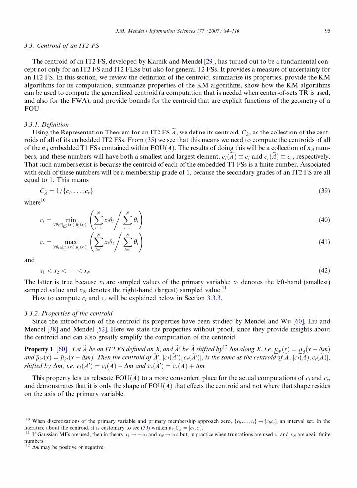
3.3. Centroid of an IT2 FS

The centroid of an IT2 FS, developed by Karnik and Mendel [29], has turned out to be a fundamental con-cept not only for an IT2 FS and IT2 FLSs but also for general T2 FSs. It provides a measure of uncertainty foran IT2 FS. In this section, we review the definition of the centroid, summarize its properties, provide the KMalgorithms for its computation, summarize properties of the KM algorithms, show how the KM algorithmscan be used to compute the generalized centroid (a computation that is needed when center-of-sets TR is used,and also for the FWA), and provide bounds for the centroid that are explicit functions of the geometry of aFOU.

3.3.1. Definition

Using the Representation Theorem for an IT2 FS eA, we define its centroid, C~A, as the collection of the cent-roids of all of its embedded IT2 FSs. From (35) we see that this means we need to compute the centroids of allof the nA embedded T1 FSs contained within FOUðeAÞ. The results of doing this will be a collection of nA num-

bers, and these numbers will have both a smallest and largest element, clðeAÞ � cl and crðeAÞ � cr, respectively.That such numbers exist is because the centroid of each of the embedded T1 FSs is a finite number. Associatedwith each of these numbers will be a membership grade of 1, because the secondary grades of an IT2 FS are allequal to 1. This means

10 Whliteratu11 If G

numbe12 Dm

C~A ¼ 1=fcl; . . . ; crg ð39Þ
where10
cl ¼ min8hi2½l~AðxiÞ;�l~AðxiÞ�

XN

i¼1

xihi

,XN

i¼1

hi

!ð40Þ

cr ¼ max8hi2½l~AðxiÞ;�l~AðxiÞ�

XN

i¼1

xihi

,XN

i¼1

hi

!ð41Þ

and

x1 < x2 < � � � < xN ð42Þ
The latter is true because xi are sampled values of the primary variable; x1 denotes the left-hand (smallest)sampled value and xN denotes the right-hand (largest) sampled value.11
How to compute cl and cr will be explained below in Section 3.3.3.

3.3.2. Properties of the centroid

Since the introduction of the centroid its properties have been studied by Mendel and Wu [60], Liu andMendel [38] and Mendel [52]. Here we state the properties without proof, since they provide insights aboutthe centroid and can also greatly simplify the computation of the centroid.

Property 1 [60]. Let eA be an IT2 FS defined on X, and eA0 be eA shifted by12 Dm along X, i.e. l~A0 ðxÞ ¼ l~Aðx� DmÞand �l~A0 ðxÞ ¼ �l~A0 ðx� DmÞ. Then the centroid of eA0, ½clðeA0Þ; crðeA0Þ�, is the same as the centroid of eA, ½clðeAÞ; crðeAÞ�,shifted by Dm, i.e. clðeA0Þ ¼ clðeAÞ þ Dm and crðeA0Þ ¼ crðeAÞ þ Dm.

This property lets us relocate FOUðeAÞ to a more convenient place for the actual computations of cl and cr,and demonstrates that it is only the shape of FOUðeAÞ that effects the centroid and not where that shape resideson the axis of the primary variable.

en discretizations of the primary variable and primary membership approach zero, {cl, . . . ,cr}! [cl,cr], an interval set. In there about the centroid, it is customary to see (39) written as C~A ¼ ½cl; cr�.aussian MFs are used, then in theory x1!�1 and xN!1; but, in practice when truncations are used x1 and xN are again finite

rs.may be positive or negative.


Property 2 [60]

(a) If FOUðeAÞ is amplitude scaled by k, where 0 < k < 1, meaning that FOUðeAÞ ! kFOUðeAÞ [i.e.,�l~A0 ðxÞ ¼ k�l~AðxÞ and l~A0 ðxÞ ¼ kl~AðxÞ] then the centroid is FOU scale-invariant.

(b) If FOUðeAÞ is shifted vertically by a constant amount [i.e., �l~A0 ðxÞ ¼ �l~AðxÞ þ d and l~A0 ðxÞ ¼ l~AðxÞ þ d] then

the centroid is not vertically shift-invariant.

(c) If the primary variable x is uniformly scaled to x/c, where c > 0 [i.e., �l~A0 ðxÞ ¼ �l~Aðx=kÞ and

l~A0 ðxÞ ¼ l~Aðx=kÞ] then the centroid scales by c to c½clðeAÞ; crðeAÞ�.When compared with Property 1 , Property 2 alerts us to the fact that the centroid is not always invariant.

Property 3 [60]. If the primary variable (x) is bounded, i.e. x 2 [x1, xN], then clðeAÞP x1 and crðeAÞ 6 xN .

Although we cannot compute the centroid in closed form, this property provides bounds for the centroidthat are available from a priori knowledge of the domain of the primary variable.

Property 4 [60]. If LMFðeAÞ is entirely on the primary-variable (x) axis, and x 2 [x1, xN], then the centroid does

not depend upon the shape of FOUðeAÞ and, as the sampling approaches zero, it equals [x1, xN].

Any FOU whose LMF is entirely on the primary-variable axis is said to be completely filled-in. This prop-erty demonstrates that for such a FOU its UMF plays no role in determining the centroid.

Property 5 [52]. If eA is symmetrical about primary variable x at x = m, then the centroid of such an IT2 FS issymmetrical about x = m, and the average value (i.e., the defuzzified value) of all the elements in the centroid

equals m.

Note that by using Property 5, we only have to compute cl, because crðeAÞ ¼ 2m� clðeAÞ. This represents a50% savings in computation. Note, also, that if one is planning only to use the defuzzified value of a symmet-rical IT2 FS, then to carry out T2 computations is a wasted effort, because the same results could have beenobtained by using T1 calculations. Fortunately (see [52] for a complete discussion), in an IT2 FLS in whichtwo or more rules are fired this sort of symmetry is not encountered. It is encountered only when one ruleis fired.

Property 6 [60]. If eA is symmetrical about m 2 X, then clðeAÞ 6 m and crðeAÞP m.

This property can be combined with Property 3 to provide lower and upper bounds for clðeAÞ and crðeAÞ.Tighter bounds will be presented below in Section 3.3.5.

Property 7 [29]. It is true that

clðeAÞ � cl ¼PkL

i¼1xi�l~AðxiÞ þPN

i¼kLþ1xil~AðxiÞPkLi¼1�l~AðxiÞ þ

PNi¼kLþ1l~AðxiÞ

ð43Þ

crðeAÞ � cr ¼PkR

i¼1xil~AðxiÞ þPn

i¼kRþ1xi�l~AðxiÞPkRi¼1l~AðxiÞ þ

Pni¼kRþ1�l~AðxiÞ

ð44Þ

where kL and kR are switch points that are computed using the KM algorithms, which are described in Section

3.3.3.

This property provides us with formulas to express clðeAÞ and crðeAÞ, even when kL and kR are not known apriori.

For our next three properties, we let

clðkÞ �Pk

i¼1xi�l~AðxiÞ þPN

i¼kþ1xil~AðxiÞPki¼1�l~AðxiÞ þ

PNi¼kþ1l~AðxiÞ

ð45Þ


Property 8 (Location of cl [38]). When k = kL, then cl(kL) = cl and xkL 6 cl < xkLþ1.

The continuous version of this property [60] is rather amazing, and is xkL ¼ cl, which means that the left-endswitch point equals the left end-point of the centroid.

Property 9 (Location of cl(k) in relation to the line y = xk [38]). It is true that cl(k) > xk when xk < cl, andcl(k) < xk when xk > cl.

This property does not imply cl(k) is monotonic on either side of cl; but, it does demonstrate that cl(k) can-not be above the line y = xk to the right of cl.

Property 10 (Monotonicity of cl(k) [38]). It is true that cl(k � 1) P cl(k) when xk < cl, and cl(k + 1) P cl(k)

when xk > cl.

This property shows that cl(k) is a monotonic function (but not a strictly-monotonic function) on both sidesof the minimum cl.

Properties very similar to Properties 8–10 also exist for cr. Simply replace cl(k), cl and kL by cr(k), cr and kU,respectively.

3.3.3. Computing the centroid using the KM algorithms

The centroid of an IT2 FS cannot be computed in closed form.13 Instead iterative algorithms developed byKarnik and Mendel [29], now known as the KM algorithms, are used. We provide statements of these algo-rithms next.

KM Algorithm for clðeAÞ: The five steps of this algorithm are (1) In (40), initialize hi by settinghi ¼ ½l~AðxiÞ þ �l~AðxiÞ�=2, i = 1, . . . ,N, and then compute c0 ¼ cðh1; . . . ; hN Þ ¼

PNi¼1xihi=

PNi¼1hi. (2) Find k

(1 6 k 6 N � 1) such that xk 6 c 0 6 xk+1. (3) Set hi ¼ �l~AðxiÞ when i 6 k, and hi ¼ l~AðxiÞ when i P k + 1,and then compute cl(k) in (45). (4) Check if cl(k) = c 0. If yes, stop and set cl(k) = cl and call k kL. If no, goto Step 5. (5) Set c 0 = cl(k) and go to Step 2.

KM Algorithm for crðeAÞ: Steps 1 and 2 are the same as in the previous algorithm, but they are for (41); (3)Set hi ¼ l~AðxiÞ when i 6 k, and hi ¼ �l~AðxiÞ when i P k + 1, and then compute

13 On

crðkÞ ¼Pk

i¼1xil~AðxiÞ þPN

i¼kþ1xi�l~AðxiÞPki¼1l~AðxiÞ þ

PNi¼kþ1�l~AðxiÞ

ð46Þ

(4) Check if cr(k) = c 0. If yes, stop and set cr(k) = cr and call k kR. If no, go to Step 5. (5) Set c 0 = cr(k) and goto Step 2.

Mendel and Liu [56] have proven that the KM algorithms are monotonically convergent and that they con-verge super-exponentially fast. Both properties are highly desirable for iterative algorithms and explain why inpractice the KM algorithms have been observed to converge very fast, thereby making them very practical touse. Prior to these results, the only available convergence statement for them was very pessimistic [29] namelyconvergence occurs in at most N iterations where N equals the number of sampled values of the primary var-iable; as N increases this bound becomes very uninformative.

3.3.4. Generalized centroid

In the following weighted average

yðz1; . . . ; zN ;w1; . . . ;wN Þ ¼PN

l¼1zlwlPNl¼1wl

ð47Þ

if each zl is replaced by an interval set zi 2 [ai, bi] and each wl is also replaced by an interval set wi 2 [ci, di], then(47) is called a generalized centroid (GC) and GC is the interval set GC = [yl, yr]. The GC is used to performcenter-of-sets TR, and is also used to compute the FWA. Because zi only appears in the numerator of (47), it iseasy to show that

e exception to this is the centroid of a fuzzy granule, for which it is possible to compute formulas for both cl and cr [60].

14 Inmaxðxcompl


yl ¼ min8wi2½ci ;di�

XN

i¼1

aiwi

,XN

i¼1

wi

!ð48Þ

yr ¼ max8wi2½ci ;di �

XN

i¼1

biwi

,XN

i¼1

wi

!ð49Þ

Comparing (48) with (40), we see that yl can be computed using the KM algorithm stated above for cl in whichxi is replaced by ai, and l~AðxiÞ and �l~AðxiÞ are replaced by ci and di, respectively. Similarly, comparing (49) with(41), we see that yr can be computed using the KM algorithm stated above for cr in which xi is replaced by bi,and again l~AðxiÞ and �l~AðxiÞ are replaced by ci and di, respectively.

3.3.5. Centroid bounds

We have seen that an IT2 FS is characterized by its FOU, which in turn is characterized by its upper andlower MFs. Wu and Mendel [95] showed that the centroid provides a measure of the uncertainty for an IT2FS. Intuitively, we anticipate that geometric properties about the FOU, such as its area and the center of grav-ities (centroids) of its upper and lower MFs, will be associated with the amount of uncertainty in such a T2 FS.Recently, Mendel and Wu [57] demonstrated that this intuition is correct. They quantified uncertainty boundsfor the centroid of both symmetric and non-symmetric IT2 FSs with respect to such geometric properties.Using these results, it is possible to formulate and solve forward problems, i.e. to go from parametric IT2FS models to data with associated uncertainty bounds. Here we only state results for a symmetrical FOU.

The geometric properties that we shall make use of, for a FOU that is symmetric about m, are AUMF, thearea under the upper MF; ALMF, the area under the lower MF; AFOU, the area of the FOU, where

AFOU ¼ AUMF � ALMF ¼ 2

Z 1

m½�lðxÞ � lðxÞ�dx; ð50Þ

and, cHFOUðeAÞ, the centroid of half of FOUðeAÞ, where

cHFOUðeAÞ ¼ R1m x½�lðxÞ � lðxÞ�dxR1m ½�lðxÞ � lðxÞ�dx

¼R1

m x½�lðxÞ � lðxÞ�dx

AFOU=2: ð51Þ

Theorem 2 [57]. Let [x1, xN] be the primary domain of eA. Then the end-points, cl and cr, for the centroid of a

symmetric IT2 FS, eA, are bounded from below and above by (Fig. 2).14

maxðx1; clðeAÞÞ 6 clðeAÞ 6 �clðeAÞ ð52ÞcrðeAÞ 6 crðeAÞ 6 minð�crðeAÞ; xNÞ ð53Þ

where

crðeAÞ ¼ mþ ½cHFOUðeAÞ � m� AFOU

AUMF þ ALMF

ð54Þ

�crðeAÞ ¼ mþ ½cHFOUðeAÞ � m� AFOU

2ALMF

ð55Þ

�clðeAÞ ¼ 2m� crðeAÞ ð56ÞclðeAÞ ¼ 2m� �crðeAÞ ð57Þ

We return to the use of these bounds in Section 5 where they will be used to solve inverse problems, i.e.going from interval data about a word to a FOU for that word.

general, �1 < x1 < xN <1, e.g. if the primary MF is Gaussian, then its associated FOU extends to ±1, in which case,

1; clðeAÞÞ ¼ clðeAÞ and minð�crðeAÞ; xN Þ ¼ �crðeAÞ. For most other FOUs, x1 and xN are finite numbers, and we need to use the moreete bounds in (52) and (53).

cl cr

xmc l cl

cl c l cr c r

crc r

−−

Fig. 2. End-points (X) of the centroid [cl, cr] of eA for a FOU that is symmetrical about m, and the lower and upper bounds (j) for the twoend-points.


3.4. Interval T2 FLSs

To-date, because of the computational complexity of using a general T2 FS in a T2 FLS, most people onlyuse an IT2 FS, the result being an IT2 FLS. Unfortunately, there is a heavy educational burden on the prac-titioner even to using an IT2 FLS. This burden has to do with first learning general T2 FS mathematics, andthen specializing it to an IT2 FS. In retrospect, requiring a person to use T2 FS mathematics represents a bar-rier to the use of an IT2 FLS. Mendel et al. [55] demonstrate that it is unnecessary to take the route from gen-eral T2 FS to IT2 FS, and that all of the results that are needed to implement an IT2 FLS can be obtainedusing T1 FS mathematics. Their paper is a very simple way for someone who is new to the field of an IT2FLS to get into it very quickly.

When all T2 FSs are IT2 FSs, then the firing set (21) and fired-rule output sets (20) are IT2 FSs, and thissimplifies all computations enormously. More specifically, for an interval singleton T2 FLS [34]: (a) the firingset becomes a firing interval, i.e.

upi¼1l~F l

iðx0iÞ � F lðx0Þ ¼ ½f lðx0Þ; �f lðx0Þ� � ½f l; �f l� ð58Þ

where

f lðx0Þ ¼ l~F l1ðx01ÞH � � �Hl~F l

pðx0pÞ ð59Þ

�f lðx0Þ ¼ �l~F l1ðx01ÞH � � �H�l~F l

pðx0pÞ ð60Þ

(b) The rule Rl fired output consequent set, l~BlðyÞ in (20), is the IT2 FS

l~BlðyÞ ¼Z

bl2½f lHl~Gl ðyÞ;�f lH�l~Gl ðyÞ�1=bl; y 2 Y ð61Þ

where l~GlðyÞ and �l~GlðyÞ are the lower and upper membership grades of l~GlðyÞ.These results have been very widely used in all applications of IT2 FLSs; however, there still may be a prob-

lem to use an IT2 FLS for real-time applications, because of the computational bottleneck of TR. Variousapproaches have been reported on for bypassing TR, some of which are summarized next.

3.5. Type-reduction and bypassing it for IT2 FLSs

When Karnik and Mendel [29] introduced TR they required adherence to the following:

Design requirement: If all sources of uncertainty disappear then a T2 FLS must reduce to a T1 FLS.

This seems like a very reasonable requirement; however, because TR may be a computational bottleneckeven for an IT2 FLS, we need to question whether or not TR is really needed.

While it is true that when all sources of uncertainty disappear, Karnik and Mendel’s TR methods reduce totheir T1 defuzzification counterparts, thereby ensuring that their IT2 FLS reduces to a T1 FLS, this does not


necessarily mean that TR is the only way for this design requirement to be met. For example, suppose that wehave computed the union of fired rule output sets, to obtain15 l~BðyÞ in (23), i.e. [34,47] (N 6M)

15 An16 We

l~BðyÞ ¼Z

b2½½f 1Hl~G1 ðyÞ�_��_½f N Hl~GN ðyÞ�;½�f 1H�l~G1 ðyÞ�_��_½�f N H�l~GN ðyÞ��1=b; y 2 Y

Let COGðl~BðyÞÞ and COGð�l~BðyÞÞ denote the centroids of the LMF and UMF, respectively, of l~BðyÞ. Then, wecan define the output of an IT2 FLS, y(x), as

yðxÞ � wCOGðl~BðyÞÞ þ ð1� wÞCOGð�l~BðyÞÞ ð62Þ

where weight w 2 [0,1] and can be tuned during a design procedure. Observe that, when all sources of uncer-tainty disappear, so that l~BðyÞ ¼ �l~BðyÞ ¼ lBðyÞ, (62) reduces to

yðxÞ ¼ COGðlBðyÞÞ ð63Þ
as required by the above Design Requirement. Similar results can be obtained for other kinds of defuzzifiers(e.g., center-of-sets defuzzification), and we leave them to the reader.
Niewiadomski et al. [67] have defined four other kinds of TR, TRoptðeBÞ, TRpesðeBÞ, TRreðeBÞ and TRrewðeBÞ,where the lower indices mean: opt—optimistic, pes—pessimistic, re—realistic, and rew—realistic-weighted, and:

TRoptðeBÞ ¼ �l~BðyÞ 8y 2 Y ð64ÞTRpesðeBÞ ¼ l~BðyÞ 8y 2 Y ð65Þ

TRreðeBÞ ¼ 1

2½l~BðyÞ þ �l~BðyÞ� 8y 2 Y ð66Þ

TRrewðeBÞ ¼ wl~BðyÞ þ ð1� wÞ�l~BðyÞ 8y 2 Y ð67Þ

Each of the functions in (64)–(67) is a T1 FS. Observe that when all sources of uncertainty disappear, so thatl~BðyÞ ¼ �l~BðyÞ ¼ lBðyÞ, then

TRoptðeBÞ ¼ TRpesðeBÞ ¼ TRreðeBÞ ¼ TRrewðeBÞ ¼ lBðyÞ 8y 2 Y ð68Þ
also as required by the above Design Requirement.
Observe also that (62) and (67) look similar, in that they both involve lower and upper MFs of l~BðyÞ, butthey are conceptually quite different, i.e. (62) by-passes TR completely, whereas (67) does not. Using (67), wecould of course compute y(x) as, e.g. yðxÞ ¼ COGðTRrewðeBÞÞ.

Gorzalczany [19,20] introduced the following interesting function of16 l~BðyÞ and �l~BðyÞ:

f ðyÞ � 1

2½l~BðyÞ þ �l~BðyÞ� � f1� ½�l~BðyÞ � l~BðyÞ�g 8y 2 Y ð69Þ

in which he calls ½�l~BðyÞ � l~BðyÞ� the ‘‘bandwidth’’ of l~BðyÞ. He then suggests two ways to compute y(x) fromf(y):

y1ðxÞ ¼ arg max8y2Y

f ðyÞ ð70Þ

y2ðxÞ ¼ median ðf ðyÞÞ ð71Þ

Observe that when all sources of uncertainty disappear, so that l~BðyÞ ¼ �l~BðyÞ ¼ lBðyÞ, then

f ðyÞ ¼ lBðyÞ 8y 2 Y ; ð72Þ
again, as required.
So now it seems that we have numerous ways to bypass TR and obtain a defuzzified output, all of whichsatisfy the basic requirement stated above. Which of these ways is best in some sense is an open question.

explicit formula for l~BðyÞ can be found in [34] and [47, Eq. (10-30)].are explaining his function using our notation, which is quite different from his notation.


There is still a problem. For random systems, we usually require both the mean and standard deviation.The latter is extremely important because it provides a measure of dispersion about the mean, and the larger(smaller) the random uncertainty, the larger (smaller) the dispersion. Mendel [47, pp. 8–9] argues that weshould not expect less of a FLS, i.e. if we view the defuzzified output of a T2 FLS as analogous to the mean,we also need a measure of dispersion about the defuzzified output, something that is analogous to standarddeviation. The Karnik-Mendel TR set provides such an uncertainty measure, but all of the above approachesdo not (yet) lead to such a measure. How to obtain a measure (or measures) of uncertainty for TRoptðeBÞ,TRpesðeBÞ, TRreðeBÞ, TRrewðeBÞ, and f(y) is an open question. If such a measure will require numerical integra-tion (e.g., like an integrated-squared error), then the computational cost for doing this should be comparedagainst the computational cost for TR performed using the KM algorithms.

An interesting alternative to inventing new kinds of TR has been provided by Wu and Mendel [95]. In theirapproach, they replace TR with lower and upper bounds—uncertainty bounds—for the end-points of the TRset, and those bounds, which are optimal in a minimax sense, can be computed without having to performTR.17 Because these uncertainty bounds have been used in some other approaches to bypassing TR (describedbelow after (87)), we state them next.

To begin, four centroids (also called boundary T1 FLSs) are defined, all of which can be computed once fl

and �f l (l = 1, . . . ,M) have been computed. In these centroids, yil and yi

r are the left- and right-end points of thecentroid of the ith consequent IT2 FS. These consequent centroids only have to be computed (and stored) onetime after the IT2 FLS has been designed, since they do not depend upon the input to the FLS. Note, e.g. thatin (73) {LMF, left} refers to the fact that this centroid only uses lower MFs of the firing interval and left-endpoint values of the consequent set centroid.

17 InMFs b

fLMFs; leftg : yð0Þl ðxÞ ¼XM

i¼1

f iyil

,XM

i¼1

f i ð73Þ

fLMFs; rightg : yðMÞr ðxÞ ¼XM

i¼1

f iyir

,XM

i¼1

f i ð74Þ

fUMFs; leftg : yðMÞl ðxÞ ¼XM

i¼1

�f iyil

,XM

i¼1

�f i ð75Þ

fUMFs; rightg : yð0Þr ðxÞ ¼XM

i¼1

�f iyir

,XM

i¼1

�f i ð76Þ

Uncertainty bounds are provided in the following:

Theorem 3 (Minimax uncertainty bounds [95]). The end-points yl(x) and yr(x) of the TR set of an IT2 FLS for

the input x, are bounded from below and above by ylðxÞ 6 ylðxÞ 6 �ylðxÞ and yrðxÞ 6 yrðxÞ 6 �yrðxÞ, where:

�ylðxÞ ¼ min yð0Þl ðxÞ; yðMÞl ðxÞ

n oð77Þ

yrðxÞ ¼ max yð0Þr ðxÞ; yðMÞr ðxÞ� �

ð78Þ

ylðxÞ ¼ �ylðxÞ �PM

i¼1ð�f i � f iÞPMi¼1

�f iPM

i¼1f i�

PMi¼1f iðyi

l � y1l ÞPM

i¼1�f iðyM

l � yilÞPM

i¼1f iðyil � y1

l Þ þPM

i¼1�f iðyM

l � yilÞ

" #ð79Þ

�yrðxÞ ¼ yrðxÞ þPM

i¼1ð�f i � f iÞPMi¼1

�f iPM

i¼1f i�

PMi¼1

�f iðyir � y1

r ÞPM

i¼1f iðyMr � yi

rÞPMi¼1

�f iðyir � y1

r Þ þPM

i¼1f iðyMr � yi

rÞ

" #ð80Þ

Observe that the four bounds in (77)–(80) can be computed without having to perform TR. Wu and Mendelthen approximate the TR set, as

[95] there are detailed derivations of the uncertainty bounds for center-of-sets TR (because it handles non-symmetrical shoulderetter than do other kinds of TR); however, these results are also applicable to other kinds of TR, as explained in [95, Table V].


½ylðxÞ; yrðxÞ� ½ðylðxÞ þ �ylðxÞÞ=2; ðyrðxÞ þ �yrðxÞÞ=2� ð81Þ

and compute the output of the IT2 FLS as

yðxÞ ¼ 1

2½ðylðxÞ þ �ylðxÞÞ=2þ ðyrðxÞ þ �yrðxÞÞ=2� ð82Þ

(instead of as (yl(x) + yr(x))/2). So, by using the uncertainty bounds, they obtain both an approximate TR set as

well as a defuzzified output. They show that

Corollary 2 [95]. The difference d(x) between the defuzzified outputs of the TR set and its approximation set for

the input x, which is defined as

dðxÞ ¼ ylðxÞ þ yrðxÞ2

� 1

2

ylðxÞ þ �ylðxÞ2

þyrðxÞ þ �yrðxÞ

2

� �� ð83Þ

is bounded from above as

dðxÞ 6 1

4½ð�ylðxÞ � ylðxÞÞ þ ð�yrðxÞ � yrðxÞÞ� ð84Þ

The next theorem helps to justify bypassing TR during the operational stage of an IT2 FLS:

Theorem 4 [95]. For a group of input–output data fxi; yigNi¼1 and an IT2 FLS, let the risk function (i.e., the

sample mean of the squared error), RTR, associated with the TR set [yl(x), yr(x)] be given as

RTR ¼1

N

XN

i¼1

yi �ylðxiÞ þ yrðxiÞ

2

� �2

ð85Þ

and the risk function, RAPP, associated with its approximation set ½ðylðxÞ þ �ylðxÞÞ=2; ðyrðxÞ þ �yrðxÞÞ=2�, be given

as

RAPP ¼1

N

XN

i¼1

yi �1

2

ylðxiÞ þ �ylðxiÞ2

þyrðxiÞ þ �yrðxiÞ

2

� �� 2

ð86Þ

Then

ffiffiffiffiffiffiffiffiRTR

p�

ffiffiffiffiffiffiffiffiffiffiRAPP

p�� 6 1

4

ffiffiffiffiffiffiffiffiffiffiffiffiffiffiffiffiffiffiffiffiffiffiffiffiffiffiffiffiffiffiffiffiffiffiffiffiffiffiffiffiffiffiffiffiffiffiffiffiffiffiffiffiffiffiffiffiffiffiffiffiffiffiffiffiffiffiffiffiffiffiffiffiffiffiffiffiffiffiffiffiffiffiffiffiffiffiffi1

N

XN

i¼1

½ð�ylðxiÞ � ylðxiÞÞ þ ð�yrðxiÞ � yrðxiÞÞ�2vuut ð87Þ

Beginning with Theorem 3 and Corollary 2, three approaches for eliminating TR have been proposed:

1. Wu and Mendel [95] use TR during the design of the IT2 FLS but then run the IT2 FLS using (77)–(82).During the design, instead of only using RTR, they use a weighted average between RTR and the Nd2(xi),i = 1, . . . ,N. In this way, they trade off some RMSE with not having to perform TR. The drawback to thisapproach is that TR is still performed during the design step.

2. Lynch et al. [40] abandon TR completely. They replace all of the IT2 FLS computations with those in (77)–(82), i.e. (77)–(82) are their IT2 FLS. Their design of this IT2 FLS is then based on minimizing RAPP. Theyfound that the errors incurred by doing this are extremely small. This is a very clever approach.

3. Melgerejo et al. [42,43] and Melgerejo and Penha-Reyes [41] have designed a VLSI IT2 FLS chip (see Sec-tion 3.6). It is also based on (77)–(82), and the Wu–Mendel design and implementation approach; however,it could also be based on the Lynch et al. approach. Because (77)–(82) are hard-wired, the design stage canbe done very quickly.

Wu and Tan [94] have approached the elimination of TR from a very different point of view. To begin, theydefine equivalent type-1 sets (ET1S) as ‘‘the collection of type-1 sets that can be used in place of the FOUs ina type 2 FLS’’. They state: ‘‘The key idea behind the proposed type-reducer is to view a T2 set as being


equivalent to a collection of ET1Ss. TR is then simplified to finding the ET1S corresponding to a particularinput. More specifically, the type-reducer needs to identify the equivalent T1 membership grade (feq) for eachinterval firing-strength. Once the equivalent T1 membership grade has been deduced, the firing set of a T2 FSreduces to a crisp value and a traditional fuzzy inference engine and defuzzifier can be employed to find theoutput of the T2 FLS. In summary, the proposed TR procedure is applied before the inference engine . . .’’.Even though they refer to this as a ‘‘proposed type-reducer’’, it is not actually TR (as they have noted) becauseit does not lead to a TR interval; hence, ‘‘it does not allow the uncertainties to flow to the inference engine. . .’’. It is, in effect, a new kind of defuzzification strategy that is able to bypass TR. They claim that thisapproach is very fast and the ‘‘. . . computational load is reduced because the inference engine behaves likethe one in a T1 FLS’’. So far, they have demonstrated this ET1S methodology for a two-input PI controller.Whether or not this methodology generalizes to more complicated systems is an open question.

3.6. Hardware realization of an IT2 FLS

One of the reasons that T1 FLSs became so widely used is that in the 1980s Takagi developed the so-calledfuzzy chip. This made it possible to implement T1 FL in hardware, which in turn led to commercialization ofFL products. Recently, Melgarejo et al. [42,43] and Melgarejo and Penha-Reyes [41] have proposed a hard-ware architecture for an already-designed IT2 FLS, one that uses the Wu–Mendel uncertainty bounds asTR [(77)–(82)] instead of the KM algorithm for TR, and also the minimum t-norm. According to [41], ‘‘ Dis-tributed arithmetic is proposed for efficiently computing on hardware the type-reduction stage . . . [and there isa] reconfigurable rule base, which is implemented in FPGA (Field Programmable Gate Array) technology.Results show that the processor performs more than 30 million of type-2 fuzzy inferences per second’’.

4. The fuzzy weighted average (FWA) and TR

The FWA is a weighted average involving T1 FSs. It has been studied in multiple criteria decision making[12,15,22,23,33,37] and is useful as an aggregation (fusion) method in situations where [see (88)] decisions (xi)and expert weights (wi) are modeled as T1 FSs, or where the decisions are modeled as either crisp numbers orinterval sets, and the expert weights are still modeled as T1 FSs.

Sometimes the same or similar problem is solved in different settings. This is the case for computing theFWA and the GC of IT2 FSs, which is why we are discussing it in this paper. Consider the following weighted

average:

y ¼Xn

i¼1

wixi

,Xn

i¼1

wi ¼ f ðw1; . . . ;wn; x1; . . . ; xnÞ ð88Þ

In (88), wi are weights that act upon attributes (indicators, features, decisions, etc.), xi. In the FWA, "xi are T1fuzzy numbers, i.e. each xi is described by the MF of a T1 FS, lX i

ðxiÞ, that must be pre-specified, and "wi arealso T1 fuzzy numbers, i.e. each wi is described by the MF of a T1 FS, lW i

ðwiÞ, that must also be pre-specified.In (88), y is a T1 FS, with MF lY(y), but there is no known closed-form formula for computing lY(y). Instead,a-cuts, an a-cut Decomposition Theorem [30] of a T1 FS, and a variety of algorithms can be used to computelY(y) (e.g., [23,37,33]).

When a-cuts are used to compute the FWA, the complete range of the membership [0,1] of the fuzzy num-bers is discretized into the following finite number of m a-cuts, a1, . . . ,am, where the degree of accuracydepends on the number of a-cuts, i.e. m. For each aj, the corresponding intervals for Xi in xi and Wi in wi

are found. The end-points of the intervals of xi and wi (i = 1, . . . ,n) are denoted by [ai(aj), bi(aj)] and [ci(aj),di(aj)], respectively. Using these a-cuts, one computes the corresponding a-cut of y, namely y(aj), i.e.

yðajÞ ¼ ½f �L ðajÞ; f �R ðajÞ� ð89Þ

lY(y) is then computed using y(a1), . . . ,y(am) as follows. Following [30], let IajYðyÞ denote the indicator

function:

Fig. 3.come o


IajYðyÞ ¼

1 8y 2 ½f �L ðajÞ; f �R ðajÞ�0 8y 62 ½f �L ðajÞ; f �R ðajÞ�

�ð90Þ

Then

lY ðyÞ ¼ sup8aj2½0;1�ðj¼1;...;mÞ

ajIajYðyÞ ð91Þ

Liou and Wang [37] were the first to observe that since the xi appear only in the numerator of (88), only thesmallest values of the xi are used to find the smallest value of (88), and only the largest values of the xi are usedto find the largest value of (88); hence,

f �L ðajÞ ¼ min8xi2½aiðajÞ;biðajÞ�8wi2½ciðajÞ;diðajÞ�

f ðw1; . . . ;wn; x1; . . . ; xnjajÞ ¼ min8wi2½ciðajÞ;diðajÞ�

f ðw1; . . . ;wn; a1; . . . ; anjajÞ ð92Þ

where

f ðw1; . . . ;wn; a1; . . . ; anjajÞ ¼Xn

i¼1

wiðajÞaiðajÞ,Xn

i¼1

wiðajÞ ð93Þ

and

f �R ðajÞ ¼ max8xi2½aiðajÞ;biðajÞ�8wi2½ciðajÞ;diðajÞ�

f ðw1; . . . ;wn; x1; . . . ; xnjajÞ ¼ max8wi2½ciðajÞ;diðajÞ�

f ðw1; . . . ;wn; b1; . . . ; bnjajÞ ð94Þ

where

f ðw1; . . . ;wn; b1; . . . ; bnjajÞ ¼Xn

i¼1

wiðajÞbiðajÞ,Xn

i¼1

wiðajÞ ð95Þ

Comparing (93) and (95) with the weighted averages in (40) and (41), respectively, we see that they are exactlythe same, provided we set hi = wi(aj) and xi = ai(aj) in (40), and hi = wi(aj) and xi = bi(aj) in (41). Consequently,the KM algorithms can be used to compute f �L ðajÞ and f �R ðajÞ. Recently, Liu and Mendel [38] have comparedthis approach to computing the FWA with Lee and Park’s Efficient FWA (EFWA) Algorithm [33] becauseprior to their work the EFWA was the fastest way to compute the FWA. Their simulations, in which ai(aj),bi(aj), ci(aj), and di(aj) were chosen randomly, all according to the same probability distribution (e.g., uniform,exponential, normal, etc.), and n was varied from 2 to 200, demonstrated that for each a-cut, convergence oc-curred (to within a 97.5% confidence interval) in three iterations, regardless of how many terms were in theFWA (i.e., n), or how ai(aj), bi(aj), ci(aj), and di(aj) were distributed, whereas the EFWA algorithm converged

yiy1 y2 yN N1 y−

μB (y)~

Hypothetical combined rule output set for a general T2 FLS. At each yi there is a different secondary MF (blackened figures) thatut of the page in the third dimension.


in ln n + c iterations, where c depended on the way in which ai(aj), bi(aj), ci(aj), and di(aj) were distributed. So,a by-product of T2 works, the KM algorithms, can now be used to compute the solution to a non-T2 problem,the FWA.

The FWA can also be used to compute the TR set for general T2 FSs. Consider the general T2 FS depictedin Fig. 3, in which the filled-in figures along the primary-variable axis denote secondary MFs, which can all bedifferent. Here we are not concerned with how this T2 FS was obtained; we are only interested in how to com-pute its TR set. Instead of using, e.g. Yc(x) as expressed in (24), we define the TR set as the weighted average ofall of the sampled secondary MFs. This is a FWA in which xi are crisp (they equal yi) and wi in (88) are thesecondary MFs, which are T1 FSs. y(aj) in (89) is the jth a-cut for the TR set, but now in (93) and (95),ai(aj) = bi(aj) = yi. How to extend this discussion to other kinds of TR is straightforward and is left to thereader.

5. Computing with words

In 1996, Zadeh published his first seminal work on computing with words. Since that time entire booksand other articles have been devoted to this important subject. A small sampling of these are[31,32,46,48,49,84,90,100–102]. Mendel [50] has proposed IT2 FSs as models for words, because words meandifferent things to different people, and so a fuzzy set model for words is needed that can capture a measureof their uncertainty.

In order to establish IT2 FS models for words, we need to collect data about words from a group of sub-jects. Next, two very different approaches for doing this are described. Both approaches map data collectedfrom subjects into a parsimonious parametric model of a FOU, and illustrate the combining of fuzzy setsand statistics—type-2 fuzzistics.18

In one approach, called the person MF approach [53], we:

1. Collect person MF data (a person-MF is a FOU that a person provides on a prescribed scale for a primary-variable) that reflects both the intra- and inter-levels of uncertainties about a word, from a group of people;

2. Define an IT2 FS model for a word as a specific aggregation of all such person MFs; and3. Mathematically model and approximate this aggregation.

This approach is based on six premises:

P1. Uncertainty about a word is of two kinds: (a) intra-uncertainty, which is the uncertainty a person hasabout the word, and (b) inter-uncertainty which is the uncertainty that a group of people have aboutthe word.

P2. Intra-uncertainty about a word, A, can be modeled using an19 IT2 person FS, eAðpjÞ, where j = 1, . . . ,nA.Such an IT2 FS is completely described by its person-FOU.

P3. Inter-uncertainty about a word can be modeled by means of an equally weighted aggregation19 of eachperson’s word FS, eAðpjÞ ðj ¼ 1; 2; . . . ; nAÞ.

P4. A natural way to aggregate a group of subject’s equally weighted word FSs is by the mathematical oper-ation of the union.19

P5. When person-MFs have been collected from a sufficient number of subjects, their union will be a filled-inword FS eAFI with associated FOU—the filled-in FOU—FOUðeAFIÞ. It is assumed that fill-in hasoccurred.

18 This term was first coined in [50].19 Mendel [53] explains why an IT2 FS leads to a first-order uncertainty model and how difficult it would be to do otherwise; it explains

equal versus non-equal weighting, and why equal weighting again leads to a first-order uncertainty model and how difficult it would be todo otherwise; and, it also explains other kinds of aggregation and why the union operation seems best.


P6. A filled-in parametric model, bA, for eAFI is one that is described by two functions, a lower MF lAðxÞ andan upper MF �lAðxÞ. These functions have shapes that are chosen ahead of time (e.g., triangle, Gaussian,piecewise-linear, trapezoidal, etc.) and each shape is characterized by a small number of parameters,some or all of which may be shared by both lAðxÞ and �lAðxÞ. These parameters are fixed during somesort of design procedure.

Observe that mathematical IT2 FS models are only used at the very end of this approach.Person MFs can only be collected from people who are already very knowledgeable about a FS, and there-

fore other techniques must be established for collecting word data from the vast majority.In a second approach, called the interval end-points approach [53], we:

1. Collect interval end-point data about a word from a group of subjects;2. Establish end-point statistics for the data; and3. Map those statistics into a pre-specified parametric FOU.

This method is analogous in statistical modeling to first choosing the underlying probability distribution(i.e., data-generating model) and then fitting the parameters of that model using data and a meaningful designmethod, e.g. the method of maximum-likelihood. This method is based on the centroid bounds that weredescribed in Theorem 2 (Section 3.3.5). The details of how to perform Step 3 are in [58] for symmetric FOUsand are under study for non-symmetrical FOUs [59].

We have mentioned all of this because we believe that IT2 FSs will play a very important role in Zadeh’sparadigm of CWW, and because much more remains to be done to turn it into an operational reality.

We also wish to mention that Turksen and his students, beginning with [68,69], have written on the impor-tant problem of how to elicit information from a subject and how that information can then be mapped intothe MF of a T1 FS.20 In [84] there are some plots to show that the T1 MFs are lower and upper bounded.Although Turksen does not refer to these plots as ‘‘FOUs’’ for words, nor does he try to directly model thisuncertainty using a T2 FS, the plots are good demonstrations (confirmations) that when MF data are collectedfrom people, they lead to a FOU.

In a FL rule-based system, not only are there antecedent and consequent words, whose uncertainties havebeen modeled using T2 FSs, especially IT2 FSs, but there are also the connector words, AND/OR. Turksenand Yao [85] and Turksen (e.g., [82–84]) have argued that it is very important to model the uncertainties ofthese two connector words. His approach is based on21 Shannon’s [76] introduction of the disjunctive and con-junctive normal forms, the DNF and CNF. These forms are used in classical logic for facilitating proofs ofsome theorems, or as a tool to simplify complicated logical statements,22 e.g., we could begin with a compli-cated statement that involves many AND’s and OR’s. Such complicated expressions can actually be simplifiedby replacing the AND’s and OR’s by their normal forms, since this leads to an expansion of the original com-plicated statement and the separate terms in the expansion are simpler than in the original statement.

Turksen et al. have fuzzified the CNF and DNF to fuzzy CNF (FCNF) and FDNF. Based on the FCNFand the FDNF each AND (intersection)/OR (union) operation leads to an interval set whose computationdepends on the specific choices one makes for a t-norm or a t-conorm. So, even if antecedent and consequentsare modeled as T1 FSs, when the AND/OR operations are modeled using the FDNF and FCNF operations,the result will be an IT2 FS. Things seem to get very complicated when there is a chain of AND/OR opera-tions, as frequently occurs in many FL rules, and no results seem to have been published on how to propagatesuch a chain of normal forms.

Using FCNF and FDNF models for the AND/OR operations transforms a T1 FLS into a T2 FLS, andusing them along with interval T2 FS models for rule-words transforms an IT2 FLS into an IT3 FLS [84].How one actually computes a T3 FS and then goes from it to a number are un-researched questions.

20 See [30] for references authored by other researchers on mapping data into T1 MF models.21 The author would like to thank Prof. George Klir for providing him with historical information about the DNF and CNF.22 The author would also like to thank Prof. Gandhi Puvadda, Dept. of Electrical Engineering, University of Southern California, who

has been teaching logic design for decades, for sharing this knowledge with him.


Other approaches for modeling the uncertainties about the AND/OR connector words, such as23 paramet-ric t-norms (t-conorms), compensatory AND, and S-OWA operators, preserve all of the mathematics in theT1 domain. Additionally, when antecedents and consequents are modeled as IT2 FSs and compensatory ANDand S-OWA models are used, then all of the mathematics remains in the IT2 FS domain [97]. Although theremay be some performance advantage to modeling the AND/OR operations to account for their uncertainties,the additional computation required to implement such a system (it is non-trivial) must be justified.

When FSs are used in the CWW paradigm, then we have argued that, because words can mean differentthings to different people (and data collected from subjects supports this), we should model the antecedentand consequent words using IT2 FSs. An interesting question is ‘‘Do the AND/OR connector words alsomean different things to different people?’’ Experimental psychologists (e.g., [16]) have conducted studies intothese issues and they have arrived at some interesting conclusions, namely: (1) most people have no difficultyin understanding the AND connector, whereas (2) many people have difficulty in understanding the OR con-nector (because one must decide whether the OR is inclusive or exclusive). In fact, they have as much difficultywith OR as they do with logical implication. Based on these human-centered studies, it would seem that theCWW paradigm does not need to include an uncertainty model for the AND connector, but it may need toinclude an uncertainty model for the OR connector. Any uncertainty model should agree with a human’suncertainty about the basic words AND/OR because those are the words that they hear (read). As yet, thereis no experimental evidence that logically equivalent models such as normal forms bear a relationship to whata person hears (reads). Which model is appropriate should somehow be tested on human subjects so that itwill be in agreement with their internal uncertainty models for OR. This remains to be done.

6. Conclusions

Much research has been and is continuing to be done on both general and IT2 FSs. Works on these subjectsare now occurring worldwide. Applications are broadening, and control applications, which were the originalbread-and-butter ones for T1 FLSs, are now a major focus of attention for IT2 FLSs. Additionally, IT2 FSsare being used to implement Zadeh’s [99] CWW paradigm; but, much more work needs to be done on this.

Only time will tell whether or not taking the step from a T1 FS to a T2 FS has made a significant difference.What is needed is a mathematical theory that establishes testable conditions for when a T2 FLS will outper-form a T1 FLS. These conditions will, no doubt, depend upon how much uncertainty is present, and remain tobe developed.

Finally, it is this author’s opinion that any problem that has previously lent itself to T1 FSs, in which MFsare uncertain, is an excellent candidate for re-examination using T2 FSs.

Acknowledgement

The author wishes to thank the reviewers for their excellent suggestions that have been incorporated intothis paper.

References

[1] J.J. Buckley, Fuzzy Probabilities: New Approaches and New Applications, Physica-Verlag, New York, 2003.[2] H. Bustince, Indicator of inclusion grade for interval-valued fuzzy sets. Application to approximate reasoning based on interval-

valued fuzzy sets, Int. J. Approx. Reas. 23 (2000) 137–209.[3] O. Castillo, P. Melin, Adaptive noise cancellation using type-2 fuzzy logic and neural networks, in: Proceedings of IEEE FUZZ

Conference, Budapest, Hungary, July 2004.[4] O. Castillo, G. Huesca, F. Valdez, Evolutionary computing for optimizing type-2 fuzzy systems in intelligent control of non-linear

dynamic plants, in: Proceedings of North American Fuzzy Information Processing Society (NAFIPS), Ann Arbor, MI, June 2005,pp. 247–251.

[5] S.M. Chen, M.S. Yeh, P.Y. Hsiao, A comparison of similarity measures of fuzzy values, Fuzzy Sets Syst. 72 (1995) 79–89.

23 There are many references about these operators. They can be found, e.g. in [96].


[6] S. Coupland, R.I. John, A new and efficient method for the type-2 meet operation, in: Proceedings of IEEE FUZZ Conference,Budapest, Hungary, July 2004, pp. 959–964.

[7] S. Coupland, R.I. John, Towards more efficient type-2 fuzzy logic systems, in: Proceedings of IEEE FUZZ Conference, Reno, NV,May 2005, pp. 236–241.

[8] V. Cross, T. Sudkamp, Similarity and compatibility in fuzzy set theory, Studies in Fuzziness and Soft Computing, vol. 93, Physica-Verlag, Heidelberg, 2002.

[9] L. Di Lascio, A. Gisolfi, A. Nappi, Medical differential diagnosis through type-2 fuzzy sets, in: Proceedings of IEEE FUZZConference, Reno, NV, May 2005, pp. 371–376.

[10] F. Doctor, H. Hagras, V. Callaghan, A type-2 fuzzy embedded agent for ubiquitous computing environment, in: Proceedings ofIEEE FUZZ Conference, Budapest, Hungary, July 2004.

[11] F. Doctor, H. Hagras, V. Callaghan, A type-2 fuzzy embedded agent to realise ambient intelligence in ubiquitous computingenvironments, Informat. Sci. 171 (2005) 309–334.

[12] W.M. Dong, F.S. Wong, Fuzzy weighted averages and implementation of the extension principle, Fuzzy Sets Syst. 21 (1987) 183–199.

[13] D. Dubois, H. Prade, Operations on fuzzy numbers, Int. J. Syst. Sci. 9 (1978) 613–626.[14] D. Dubois, H. Prade, Operations in a fuzzy-valued logic, Informat. Cont. 43 (1979) 224–240.[15] D. Dubois, H. Fargier, J. Fortin, A generalized vertex method for computing with fuzzy intervals, in: Proceedings of FUZZ IEEE

2004, Budapest, Hungary, 2004, pp. 541–546.[16] J. St. B.T. Evans, S.E. Newstead, R.M.J. Byrne, Human Reasoning: The Psychology of Deduction, Lawrence Erlbaum Associates,

Hove, UK, 1993.[17] J. Figueroa, J. Posada, J. Soriano, M. Melgarejo, S. Rojas, A type-2 fuzzy controller for tracking mobile objects in the context of

robotic soccer games, in: Proceedings of IEEE FUZZ Conference, Reno, NV, May 2005, pp. 359–364.[18] J.M. Garibaldi, S. Musikasuwan, T. Ozen, The association between non-stationary and interval type-2 fuzzy sets: a case study, in:

Proceedings of IEEE FUZZ Conference, Reno, NV, May 2005, pp. 224–229.[19] M.B. Gorzalczany, Decision making in signal transmission problems with interval-valued fuzzy sets, Fuzzy Sets Syst. 23 (1987) 191–

203.[20] M.B. Gorzalczany, Interval-valued fuzzy controller based on verbal model of object, Fuzzy Sets Syst. 28 (1988) 45–53.[21] S. Greenfield, R.I. John, S. Coupland, A novel sampling method for type-2 defuzzification, submitted for publication.[22] Y.-Y. Guh, C.-C. Hon, E.S. Lee, Fuzzy weighted average: the linear programming approach via Charnes and Cooper’s rule, Fuzzy

Sets Syst. 117 (2001) 157–160.[23] Y.-Y. Guh, C.-C. Hon, K.-M. Wang, E.S. Lee, Fuzzy weighted average: a max–min paired elimination method, Comput. Math.

Appl. 32 (1996) 115–123.[24] H. Hagras, A hierarchical type-2 fuzzy logic control architecture for autonomous mobile robots, IEEE Trans. Fuzzy Syst. 12 (4)

(2004) 524–539.[25] H. Hagras, A type-2 fuzzy logic controller for autonomous mobile robots, in: Proceedings of IEEE FUZZ Conference, Budapest,

Hungary, July 2004.[26] C. Hwang, F.C.-H. Rhee, An interval type-2 fuzzy spherical shells algorithm, in: Proceedings of IEEE FUZZ Conference, Budapest,

Hungary, July 2004.[27] R.I. John, P.R. Innocent, Modeling uncertainty in clinical diagnosis using fuzzy logic, IEEE Trans. Syst., Man, Cybernet. Part B:

Cybernet. 35 (2005) 1340–1350.[28] N.N. Karnik, J.M. Mendel, Operations on type-2 fuzzy sets, Fuzzy Sets Syst. 122 (2001) 327–348.[29] N.N. Karnik, J.M. Mendel, Centroid of a type-2 fuzzy set, Informat. Sci. 132 (2001) 195–220.[30] G.J. Klir, B. Yuan, Fuzzy Sets and Fuzzy Logic: Theory and Applications, Prentice-Hall, Upper Saddle River, NJ, 1995.[31] J. Lawry, An alternative to computing with words, Int. J. Uncert. Fuzz. Know. Syst. 9 (Suppl.) (2001) 3–16.[32] J. Lawry, J. Shanahan, A. Ralescu (Eds.), Modeling With Words, Lecture Notes in Artificial Intelligence 2873, Springer, New York,

2003.[33] D.H. Lee, D. Park, An efficient algorithm for fuzzy weighted average, Fuzzy Sets Syst. 87 (1997) 39–45.[34] Q. Liang, J.M. Mendel, Interval type-2 fuzzy logic systems: theory and design, IEEE Trans. Fuzzy Syst. 8 (2000) 535–550.[35] Q. Liang, L. Wang, Sensed signal strength forecasting for wireless sensors using interval type-2 fuzzy logic system, in: Proceedings of

IEEE FUZZ Conference, Reno, NV, May 2005, pp. 25–30.[36] P.-Z. Lin, C.-F. Hsu, T.-T. Lee, Type-2 fuzzy logic controller design for buck DC–DC converters, in: Proceedings of IEEE FUZZ

Conference, Reno, NV, May 2005, pp. 365–370.[37] T.-S. Liou, M.-J.J. Wang, Fuzzy weighted average: an improved algorithm, Fuzzy Sets Syst. 49 (1992) 307–315.[38] F. Liu, J.M. Mendel, Aggregation using the fuzzy weighted average, as computed by the KM algorithms, submitted for publication.[39] L. Lushu, Random fuzzy sets and fuzzy martingales, Fuzzy Sets Syst. 69 (1995) 181–192.[40] C. Lynch, H. Hagras, V. Callaghan, Embedded type-2 FLC for real-time speed control of marine and traction diesel engines, in:

Proceedings of IEEE FUZZ Conference, Reno, NV, May 2005, pp. 347–352.[41] M.C.A. Melgarejo, C.A. Penha-Reyes, Hardware realization of an interval type-2 fuzzy inference system, IEEE Trans. Fuzzy Syst.,

in press.[42] M.C.A. Melgarejo, A. Garcia, C.A. Penha-Reyes, Pro-two: a hardware based platform for real time type-2 fuzzy inference, in:

Proceedings of IEEE FUZZ Conference, Budapest, Hungary, July 2004.


[43] M.C.A. Melgarejo, C.A. Penha-Reyes, A. Garcia, Computational model and architectural proposal for a hardware type-2 fuzzysystem, in: Proceedings of 2nd IASTED Conference Neural Network and Computational Intelligence, Grindewald, 2004, pp. 279–284.

[44] P. Melin, O. Castillo, A new method for adaptive model-based control of non-linear plants using type-2 fuzzy logic and neuralnetworks, in: Proceedings of IEEE FUZZ Conference, St. Louis, MO, May 2003, pp. 420–425.

[45] P. Melin, O. Castillo, A new approach for quality control of sound speakers combining type-2 fuzzy logic and the fractal dimension,in: Proceedings of International Conference NAFIPS 2003, Chicago, USA, July 2003, pp. 20–25.

[46] J.M. Mendel, Computing with words, when words can mean different things to different people, in: Proceedings of ThirdInternational ICSC Symposium on Fuzzy Logic and Applications, Rochester Univ., Rochester, NY, June 1999.

[47] J.M. Mendel, Uncertain Rule-Based Fuzzy Logic Systems: Introduction and New Directions, Prentice-Hall, Upper-Saddle River,NJ, 2001.

[48] J.M. Mendel, The perceptual computer: an architecture for computing with words, in: Proceedings of Modeling With WordsWorkshop in the Proceedings of FUZZ-IEEE, Melbourne, Australia, December 2001, pp. 35–38.

[49] J.M. Mendel, An architecture for making judgments using computing with words, Int. J. Appl. Math. Comput. Sci. 12 (3) (2002)325–335.

[50] J.M. Mendel, Fuzzy sets for words: a new beginning, in: Proceedings of IEEE International Conference on Fuzzy Systems, St. Louis,MO, 2003, pp. 37–42.

[51] J.M. Mendel, Type-2 fuzzy sets: some questions and answers, IEEE Connect., Newslett. IEEE Neural Networks Soc. 1 (2003) 10–13.[52] J.M. Mendel, On a 50% savings in the computation of the centroid of a symmetrical interval type-2 fuzzy set, Informat. Sci. 172

(2005) 417–430.[53] J.M. Mendel, Computing with words and its relationships with fuzzistics, Informat. Sci., in press, doi:10.1016/j.ins.2006.06.008.[54] J.M. Mendel, R.I. John, Type-2 fuzzy sets made simple, IEEE Trans. Fuzzy Syst. 10 (2002) 117–127. April 2002.[55] J.M. Mendel, R.I. John, F. Liu, Interval type-2 fuzzy logic systems made simple, IEEE Trans. Fuzzy Syst., in press.[56] J.M. Mendel, F. Liu, Super-exponential convergence of the Karnik–Mendel algorithms for computing the centroid of an interval

type-2 fuzzy set, IEEE Trans. Fuzzy Syst., in press.[57] J.M. Mendel, H. Wu, Type-2 fuzzistics for symmetric interval type-2 fuzzy sets: Part 1, forward problems, IEEE Trans. Fuzzy Syst.,

in press.[58] J.M. Mendel, H. Wu, Type-2 fuzzistics for symmetric interval type-2 fuzzy sets: Part 2, inverse problems, IEEE Trans. Fuzzy Syst., in

press.[59] J.M. Mendel, H. Wu, Type-2 fuzzistics for non-symmetric interval type-2 fuzzy sets: forward problems, IEEE Trans. Fuzzy Syst., in

press.[60] J.M. Mendel, H. Wu, New results about the centroid of an interval type-2 fuzzy set, including the centroid of a fuzzy granule,

Informat. Sci., in press, doi:10.1016/j.ins.2006.03.003.[61] G.M. Mendez, O. Castillo, Interval type-2 TSK fuzzy logic systems using hybrid learning algorithm, in: Proceedings of IEEE FUZZ

Conference, Reno, NV, May 2005, pp. 230–235.[62] H.B. Mitchell, Pattern recognition using type-II fuzzy sets, Informat. Sci. 170 (2005) 409–418.[63] M. Mizumoto, K. Tanaka, Some properties of fuzzy sets of type-2, Informat. Cont. 31 (1976) 312–340.[64] M. Mizumoto, K. Tanaka, Fuzzy sets of type-2 under algebraic product and algebraic sum, Fuzzy Sets Syst. 5 (1981) 277–290.[65] B. Moller, M. Beere, Fuzzy Randomness: Uncertainty in Civil Engineering and Computational Mechanics, Springer, New York,

2004.[66] J. Nieminen, J. On the algebraic structure of fuzzy sets of type-2, Kybernetica 13 (4) (1977).[67] A. Niewiadomski, J. Kacprzyk, J. Ochelska, P.S. Szczepaniak, Interval-valued linguistic summaries of databases, Control &

Cybernetics, Systems Research Institute, Polish Academy of Science, Warsaw, Poland, in press.[68] A.M. Norwich, I.B. Turks�en, The fundamental measurement of fuzziness, in: R.R. Yager (Ed.), Fuzzy Sets and Possibility Theory,

Pergamon Press, NY, 1982, pp. 49–60.[69] A.M. Norwich, I.B. Turks�en, A model for the measurement of membership and the consequences of its empirical implementation,

Fuzzy Sets Syst. 12 (1984) 1–25.[70] T. Ozen, J, M. Garibaldi, S. Musikasuwan, Preliminary investigations into modeling the variation in human decision making, in:

Proceedings of 10th Information Processing and Management of Uncertainty in Knowledge Based Systems (IPMU 2004), Perugia,Italy, July 2004, pp. 641–648.

[71] S. Rahimi, M. Cobb, A. Zhou, D. Ali, H. Yang, F.E. Petry, An inexact inferencing strategy for spatial objects with determined andindeterminate boundaries, in: Proceedings of IEEE FUZZ Conference, St. Louis, MO, 2003, pp. 778–783.

[72] F.C.-H. Rhee, C. Hwang, A type-2 fuzzy c-means clustering algorithm, in: Proceedings of IEEE FUZZ Conference, Melbourne,Australia, December 2001, pp. 1926–1929.

[73] F.C.-H. Rhee, C. Hwang, An interval type-2 fuzzy perceptron, in: Proceedings of IEEE FUZZ Conference, Honolulu, HI, May2002.

[74] F.C.-H. Rhee, C. Hwang, An interval type-2 fuzzy K-nearest neighbor, in: Proceedings of IEEE FUZZ Conference, Honolulu, HI,May 2002, pp. 802–807.

[75] R. Sepulveda, O. Castillo, P. Melin, A. Rodriguez-Diaz, O. Montiel, Integrated development platform for intelligent control basedon type-2 fuzzy logic, in: Proceedings of North American Fuzzy Information Processing Society (NAFIPS), Ann Arbor, MI, June,2005, pp. 607–610.

[76] C. Shannon, A symbolic analysis of relay and switching circuits, Am. Inst. Elect. Engrs. 57 (1938).

http://dx.doi.org/10.1016/j.ins.2006.06.008

http://dx.doi.org/10.1016/j.ins.2006.03.003


[77] H. Shu, Q. Liang, Wireless sensor network lifetime analysis using interval type-2 fuzzy logic systems, in: Proceedings of IEEE FUZZConference, Reno, NV, May 2005, pp. 19–24.

[78] J.T. Starczewski, Extended triangular norms, submitted for publication.[79] J.T. Starczewski, A triangular type-2 fuzzy logic system, submitted for publication.[80] J.T. Starczewski, Extended triangular norms on Gaussian fuzzy sets, in: Proceedings of EUSFLAT-LFA, Barcelona, Spain,

September 2005, pp. 872–877.[81] W.W. Tan, J. Lai, Development of a type-2 fuzzy proportional controller, in: Proceedings of IEEE FUZZ Conference, Budapest,

Hungary, July 2004.[82] I.B. Turksen, Interval-valued fuzzy sets based on normal forms, Fuzzy Sets Syst. 20 (1986) 191–210.[83] I.B. Turksen, Interval valued fuzzy sets and fuzzy connectives, J. Interval Comput. 4 (1993) 125–142.[84] I.B. Turksen, Type-2 representation and reasoning for CWW, Fuzzy Sets Syst. 127 (2002) 17–36.[85] I.B. Turksen, D.D.W. Yao, Representation of connectives in fuzzy reasoning: the view through normal forms, IEEE Trans. Syst.

Man Cybernet. 14 (1984) 146–150.[86] M. Wagenknecht, K. Hartmann, Application of fuzzy sets of type-2 to the solution of fuzzy equation systems, Fuzzy Sets Syst. 25

(1988) 183–190.[87] C. Walker, E. Walker, The algebra of fuzzy truth values, Fuzzy Sets Syst., in press.[88] C. Walker, E. Walker, Some general comments on fuzzy sets of type-2, presented at BISCSE 2005 Forging New Frontiers, 40th of

Fuzzy Pioneers, BISC Special Event in Honor of Prof. Lotfi A. Zadeh, Univ. of California, Berkeley, CA, November 2–5, 2005.[89] C. Walker, E. Walker, Automorphisms of the algebra of fuzzy truth values, in preparation.[90] P.P. Wang (Ed.), Computing With Words, John Wiley & Sons Inc, New York, 2001.[91] X. Wang, B. De Baets, E. Kerre, A comparative study of similarity measures, Fuzzy Sets Syst. 73 (1995) 259–268.[92] K. Wills, R.I. John, S. Lake, Combining categories in nursing assessment using interval valued fuzzy sets, in: Proceedings of 10th

Information Processing and Management of Uncertainty in Knowledge Based Systems (IPMU 2004), Perugia, Italy, July 2004.[93] D. Wu, W.W. Tan, A type-2 fuzzy logic controller for the liquid-level process, in: Proceedings of IEEE FUZZ Conference, Budapest,

Hungary, July 2004, pp. 953–958.[94] D. Wu, W.W. Tan, Computationally efficient type-reduction strategies for a type-2 fuzzy logic controller, in: Proceedings of IEEE

FUZZ Conference, Reno, NV, May 2005, pp. 353–358.[95] H. Wu, J.M. Mendel, Uncertainty bounds and their use in the design of interval type-2 fuzzy logic systems, IEEE Trans. Fuzzy Syst.

10 (2002) 622–639.[96] H. Wu, J.M. Mendel, On choosing models for linguistic connector words for Mamdani fuzzy logic systems, IEEE Trans. Fuzzy Syst.

12 (2004) 29–44.[97] H. Wu, J.M. Mendel, Antecedent connector word models for Interval type-2 fuzzy logic system, in: Proceedings of IEEE FUZZ

Conference, Budapest, Hungary, July 2004.[98] L.A. Zadeh, The concept of a linguistic variable and its application to approximate reasoning–1, Informat. Sci. 8 (1975) 199–249.[99] L.A. Zadeh, Fuzzy logic = computing with words, IEEE Trans. Fuzzy Syst. 4 (1996) 103–111.

[100] L.A. Zadeh, From computing with numbers to computing with words—from manipulation of measurements to manipulation ofperceptions, IEEE Trans. Circ. Syst.—I: Fundam. Theory Appl. 4 (1999) 105–119.

[101] L.A. Zadeh, Towards a generalized theory of uncertainty (GTU)–an outline, Informat. Sci. 172 (2005) 1–40, June 2005.[102] L.A. Zadeh, J. Kacprzyk (Eds.), Computing With Words in Information/Intelligent Systems 1 & 2, Physica-Verlag, New York,

1999.[103] J. Zeng, Z.-Q. Liu, Interval type-2 fuzzy hidden markov models, in: Proceedings of IEEE FUZZ Conference, Budapest, Hungary,

July 2004.

Advances in type-2 fuzzy sets and systems - AMiner · interval type-2 fuzzy sets and systems are...

Documents

Transcript of Advances in type-2 fuzzy sets and systems - AMiner · interval type-2 fuzzy sets and systems are...