ADVANCES IN LOCAL STEREOLOGYWITH EMPHASIS ON SURFACE AREA ESTIMATION AND WICKSELL’S PROBLEM

PHD THESIS BY ÓLÖF THÓRISDÓTTIR

SUPERVISED BY MARKUS KIDERLEN

SEPTEMBER 2013

DEPARTMENT OF MATHEMATICS

AARHUS UNIVERSITY

Contents

Preface v

Abstract vii

Resumé ix

Introduction 11 Stereology . . . . . . . . . . . . . . . . . . . . . . . . . . . . . . . . . . 12 Theoretical background . . . . . . . . . . . . . . . . . . . . . . . . . . 2

2.1 The intrinsic volumes . . . . . . . . . . . . . . . . . . . . . . . 32.2 Linear and affine subspaces . . . . . . . . . . . . . . . . . . . . 42.3 Blaschke-Petkantschin type measure decompositions . . . . . 4

3 Classical vs. local stereology . . . . . . . . . . . . . . . . . . . . . . . . 53.1 Geometric summary statistics . . . . . . . . . . . . . . . . . . . 63.2 Particle distributions . . . . . . . . . . . . . . . . . . . . . . . . 9

4 Motivation . . . . . . . . . . . . . . . . . . . . . . . . . . . . . . . . . . 114.1 The invariator estimator . . . . . . . . . . . . . . . . . . . . . . 114.2 Variance decomposition . . . . . . . . . . . . . . . . . . . . . . 124.3 Composition of the papers . . . . . . . . . . . . . . . . . . . . 13

5 Wicksell’s problem in local stereology . . . . . . . . . . . . . . . . . . 145.1 Local Wicksell . . . . . . . . . . . . . . . . . . . . . . . . . . . . 145.2 Reconstruction methods . . . . . . . . . . . . . . . . . . . . . . 16

6 Rotational Crofton-type formulae using the invariator principle . . . 166.1 A rotational Crofton formula involving Morse theory . . . . . 186.2 The Morse type surface area estimator . . . . . . . . . . . . . . 186.3 Flower area . . . . . . . . . . . . . . . . . . . . . . . . . . . . . 19

7 The Morse type surfacea area estimator in practice . . . . . . . . . . . 207.1 A modification of the area tangent count method . . . . . . . 207.2 Implementation of the Morse type surface area estimator . . . 21

8 Outlook . . . . . . . . . . . . . . . . . . . . . . . . . . . . . . . . . . . . 23Bibliography . . . . . . . . . . . . . . . . . . . . . . . . . . . . . . . . . . . . 24

A Wicksell’s problem in local stereology 31by Ó. Thórisdóttir and M. Kiderlen

i

Contents

A.1 Introduction and account of main results . . . . . . . . . . . . . . . . 31A.2 Preliminaries . . . . . . . . . . . . . . . . . . . . . . . . . . . . . . . . . 35A.3 The direct problem . . . . . . . . . . . . . . . . . . . . . . . . . . . . . 36A.4 Uniqueness . . . . . . . . . . . . . . . . . . . . . . . . . . . . . . . . . 40A.5 The unfolding problem . . . . . . . . . . . . . . . . . . . . . . . . . . . 42A.6 Reconstruction . . . . . . . . . . . . . . . . . . . . . . . . . . . . . . . . 44A.7 Examples . . . . . . . . . . . . . . . . . . . . . . . . . . . . . . . . . . . 47A.8 Stereology of extremes . . . . . . . . . . . . . . . . . . . . . . . . . . . 49A.9 Conclusion . . . . . . . . . . . . . . . . . . . . . . . . . . . . . . . . . . 50Appendix: S3M for FR . . . . . . . . . . . . . . . . . . . . . . . . . . . . . . . 50Bibliography . . . . . . . . . . . . . . . . . . . . . . . . . . . . . . . . . . . . 52

Supplementary material . . . . . . . . . . . . . . . . . . . . . . . . . . . . . 54A.I Extended version of Example A.8 . . . . . . . . . . . . . . . . 54A.II The constants in (A.37) . . . . . . . . . . . . . . . . . . . . . . . 55A.III Proof of Proposition A.15 . . . . . . . . . . . . . . . . . . . . . 55

B The invariator principle in convex geometry 59by Ó. Thórisdóttir and M. Kiderlen

B.1 Introduction . . . . . . . . . . . . . . . . . . . . . . . . . . . . . . . . . 59B.2 Preliminaries . . . . . . . . . . . . . . . . . . . . . . . . . . . . . . . . . 61B.3 Invariator principle and rotational Crofton formulae . . . . . . . . . . 64B.4 Representations of the measurement function . . . . . . . . . . . . . . 67

B.4.1 The measurement function as an integral over the profileboundary . . . . . . . . . . . . . . . . . . . . . . . . . . . . . . 67

B.4.2 The measurement function as an integral over the sphere . . . 68B.4.3 Morse type representation . . . . . . . . . . . . . . . . . . . . . 71B.4.4 The generalized flower volume and projection formulae . . . 76

B.5 Stereological applications . . . . . . . . . . . . . . . . . . . . . . . . . 79Bibliography . . . . . . . . . . . . . . . . . . . . . . . . . . . . . . . . . . . . 83

C Estimating the surface area of non-convex particles from central planarsections 87by Ó. Thórisdóttir, A.H. Rafati and M. Kiderlen

C.1 Introduction . . . . . . . . . . . . . . . . . . . . . . . . . . . . . . . . . 87C.2 Theoretical background . . . . . . . . . . . . . . . . . . . . . . . . . . 89

C.2.1 The invariator estimator for surface area . . . . . . . . . . . . 90C.2.2 Morse type surface area estimator . . . . . . . . . . . . . . . . 92

C.3 Variance . . . . . . . . . . . . . . . . . . . . . . . . . . . . . . . . . . . 96C.3.1 Variance decomposition . . . . . . . . . . . . . . . . . . . . . . 96C.3.2 Numerical results for ellipsoids . . . . . . . . . . . . . . . . . . 99C.3.3 Variance of the Morse type surface area estimator . . . . . . . 100C.3.4 Efficiency of the Morse type surface area estimator . . . . . . 101

C.4 Application of the Morse type surface area estimator . . . . . . . . . 105

ii

Contents

C.4.1 Model-based setting . . . . . . . . . . . . . . . . . . . . . . . . 106C.4.2 Materials and preparation methods . . . . . . . . . . . . . . . 106C.4.3 Implementation of the Morse type surface area estimator . . . 107C.4.4 Results . . . . . . . . . . . . . . . . . . . . . . . . . . . . . . . . 109

C.5 Discussion . . . . . . . . . . . . . . . . . . . . . . . . . . . . . . . . . . 111C.5.1 Account of main results . . . . . . . . . . . . . . . . . . . . . . 111C.5.2 Automatic and semi-automatic estimation of surface area . . 112

Appendix: Variance decomposition for ellipsoids . . . . . . . . . . . . . . . 113Bibliography . . . . . . . . . . . . . . . . . . . . . . . . . . . . . . . . . . . . 114

iii

Preface

Stereology concerns the estimation of geometric characteristics of spatial structuresfrom lower dimensional information about the structures. I was introduced to thefascinating and creative world of stereology in my master’s studies at AarhusUniversity, primarily through the writing of my master’s thesis. It is in particular theinterplay of geometrical and statistical issues in stereology that has a great appealto me. A more recent and less developed branch of stereology is local stereology.This thesis is a contribution to local stereology and presents the outcome of theresearch part of my PhD studies. The studies were carried out at the Department ofMathematics, Aarhus University, from October 2010 to September 2013, under thecareful supervision of Markus Kiderlen. The PhD studies were partly financed byCenter for Stochastic Geometry and Advanced Bioimaging (CSGB), funded by theVillum Foundation.

The thesis consists of three independently written and self-contained papers:

Paper A . . . . . . . . . . . . . . . . . . . . . . . . . . . . . . . . . . . . . . . . . 31Ó. Thórisdóttir and M. Kiderlen. Wicksell’s problem in local stereology.Adv. Appl. Prob. To appear, 2013.

Paper B . . . . . . . . . . . . . . . . . . . . . . . . . . . . . . . . . . . . . . . . . 59Ó. Thórisdóttir and M. Kiderlen. The invariator principle in convex geom-etry. Submitted, 2013.

Paper C . . . . . . . . . . . . . . . . . . . . . . . . . . . . . . . . . . . . . . . . . 87Ó. Thórisdóttir, Ali H. Rafati and M. Kiderlen. Estimating the surface areaof non-convex particles from central planar sections. Submitted, 2013.

Besides being submitted to international journals, all three papers can be found asCSGB research reports. The technical parts that were omitted in the accepted versionof Paper A and only included in the CSGB research report can be found as supple-mentary material on pages 54–58. The thesis also contains an introductory chapter,where the three papers are connected together, their main results summarized andtheir importance for the stereological community emphasized.

The work constituting the three papers has been presented at the followingconferences and workshops:

v

Preface

• 16th Workshop on Stochastic Geometry, Stereology and Image Analysis. Sand-bjerg, Denmark, June 2011,

• 13th International Conference on Stereology, Beijing, China, October 2011,

• 4th Internal CSGB Workshop, Aarhus, Denmark, November 2011,

• GPSRS Workshop, Erlangen, Germany, September 2012

• 6th Internal CSGB Workshop, Skagen, Denmark, May 2013

• 11th European Congress of Stereology and Image Analysis, Kaiserslautern,Germany, July 2013.

Acknowledgement

This thesis would not exist if it were not for my supervisor’s, Markus Kiderlen,sincere dedication to our work. I am indebted to him for originally encouragingme to take on the challenge of PhD studies and for continuously stimulating methroughout the studies.

I am grateful to have been a part of Eva B. Vedel Jensen’s center CSGB. Theinterdisciplinary research undertaken at the center has broadened my horizon andadded a sense of importance and practical relevance to my work. Furthermore, ithas been a privilege to work on ground-breaking research under the guidance ofoutstanding professors. Paper C is the fruit of a collaboration with the Stereologyand EM Research Laboratory, Aarhus University, and I want to thank Ali H. Rafatifor nice collaboration. I also want to acknowledge Lars Madsen’s generous supportconcerning the final layout of this thesis.

I would like to thank my dear colleagues in ‘statistisk strikkeklub’, in partic-ular Camilla Mondrup Andreassen and Ina Trolle Andersen for their invaluablesupport. Furthermore, I want to thank my family and friends and the never-failingF-myndum.

Ólöf ThórisdóttirAarhus, September 2013

vi

Abstract

This thesis presents advances in local stereology. The goal is to make statistical infer-ence about geometric characteristics of a spatial structure. The inference is typicallymade from flat sections taken through a fixed reference point of the structure. Localstereology has proven to be very useful for applications in biomedicine.

When the aim is to estimate the distribution of the particle shape from randomsamples, strict shape assumptions on the particles under study have to be imposed.There exists much literature on the classical Wicksell problem, which is concernedwith the estimation of the radius distribution of balls from the radius distribution ofisotropic uniform random (IUR) flat sections through the balls. We treat Wicksell’sclassical problem in a local setting. Here the balls are (up to rotations) characterizedby two random variables: their radius and the position of their reference pointinside the ball. We derive several results that are analogue to results for the classicalWicksell problem such as unfolding of the arising integral equations, momentrelations and stereology of extremes, but we also emphasize differences betweenthe local and the classical problem.

Without strict shape assumptions on the particles of interest, we have to settle formean geometric characteristics of the particles, instead of their distribution. Thesecharacteristics could for example be intrinsic volumes, like volume or surface area.We derive a new local stereological estimator for surface area which we call the Morsetype surface area estimator. The estimator is obtained by combining Morse theory,Crofton’s formula and the invariator principle, which is a Blaschke-Petkantschintype measure decomposition. The estimator can also be described as a modificationof the ‘area tangent count method’ in stereology. We show that the Morse typeestimator is better (in terms of efficiency and precision) than existing local surfacearea estimators and illustrate its practicability in a biological application.

The above mentioned combination of the classical Crofton formula with theinvariator principle is a powerful tool to derive rotational Crofton formulae. As rota-tional Crofton formulae in turn are the basis for local stereological estimators, wediscuss these formulae more systematically. Rotational Crofton formulae deal withsections of an object with isotropically randomized flats that pass through the origin.They answer the question which measurement function of the section to choose toobtain an unbiased estimator of a geometric characteristic of the object. We first re-view known measurement functions that yield intrinsic volumes or, more generallyMinkowski tensors. We then show that there are also rotational Crofton formulae

vii

Abstract

for support measures and curvature measures. Often, the measurement function isnot given explicitly but only as an integral geometric expression. We derive severaldifferent, more explicit representations of the measurement function. The most im-portant of these representations involves writing the measurement function in termsof so-called critical values of the section profile. This is first achieved for smoothmanifolds using Morse theory and then for polyconvex sets using Hadwiger’s index.All the different representations play an important role when rotational Croftonformulae are applied in local stereology.

viii

Resumé

Denne afhandling præsenterer fremskridt i lokal stereologi. Formålet er at lavestatistisk inferens om geometriske karakteristika af et objekt i rummet. Inferensenlaves typisk fra affine snit taget igennem et fast referencepunkt i objektet. Lokalstereologi har vist sig at være meget nyttig for anvendelser i biomedicin.

Når formålet er at estimere fordelingen af formen af partikler fra tilfældige snit, erdet nødvendigt at lægge strenge antagelser på formen af partiklerne. Der eksistereren betydelig mængde litteratur om det klassiske Wicksell-problem, som involvererestimationen af radiusfordelingen af kugler fra radiusfordelingen af isotropiskeuniforme (IUR) snit gennem kuglerne. Vi betragter Wicksells klassiske problem i etlokalt setting. Her er kuglerne (op til rotationer) karakteriserede ved to stokastiskevariable: deres radius og positionen af deres referencepunkt inden i kuglen. Viudleder adskillige resultater, der svarer til resultater for det klassiske Wicksell-problem som for eksempel inversion af de integral-ligninger der opstår, moment-relationer og stereologi af ekstremer, men vi beskriver også forskelle mellem detlokale og det klassiske problem.

Uden strenge antagelser på formen af partiklerne som vi betragter, må vi nøjesmed gennemsnittet af geometriske karakteristika, i stedet for deres fordeling. Dissekarakteristika kunne for eksempel være de indre volumina, som volumen elleroverfladeareal. Vi udleder en ny lokal stereologisk estimator for overfladearealsom vi kalder „Morse-type estimatoren af overfladeareal “. Estimatoren er baseretpå at kombinere Morse-teori, Croftons formel og invariator-princippet, som er enmåldekomposition af Blaschke-Petkantschin-type. Estimatoren kan også beskrivesved en modificering af „areal-tangent-optælningsmetoden“ i stereologi. Vi viser,at estimatoren af Morse-type er bedre (hvad angår effektivitet og præcision) endeksisterende estimatorer og illustrerer dens brugbarhed i en biologisk anvendelse.

Den ovennævnte kombination af den klassiske Crofton-formel og invariator-princippet er et nyttigt redskab for at udlede rotations-Crofton-formler. Da rotations-Crofton-formler udgør grundlaget for lokale stereologiske estimatorer, diskuterer vidisse formler mere systematisk. Rotations-Crofton-formler beskæftiger sig med snitaf objekter med isotropiske randomiserede planer, der går igennem origo. De giversvar på spørgsmålet om, hvilken målingsfunktion af snittet, der burde betragtesfor at få en middelværdiret estimator af geometriske karakteristika af objektet. Vigiver først en oversigt over kendte målingsfunktioner, der giver de indre volu-mina, eller mere generelt Minkowski-tensorer. Dernæst viser vi, at der også findes

ix

Resumé

rotations-Crofton-formler for supportmålene og krumningsmålene. Målingsfunk-tionen er ofte ikke udtrykt eksplicit men kun som et integralgeometrisk udtryk.Vi udleder adskillige forskellige mere eksplicitte repræsentationer af målingsfunk-tionen. Den mest vigtige af disse repræsentationer udtrykker målingsfunktionenved hjælp af såkaldte kristiske værdier af snit-profilen. Dette gøres først for glattemangfoldigheder ved at bruge Morse-teori og så for polykonvekse mængder ved atbruge Hadwigers indeks. Alle de forskellige repræsentationer spiller en vigtig rolle,når rotations-Crofton-formler er anvendt i lokal stereologi.

x

Introduction

The three papers that constitute this thesis are all facets of local stereology thatwere missing in the general picture. This introductory chapter serves to bind thepapers together, present their main results and emphasize their importance for thestereological community. In order to achieve this we give a few pages of introductionto stereology and important concepts in stochastic and integral geometry.

1 Stereology

The International Society for Stereology (ISS) was founded in 1961 and gatheredresearchers from as different fields as biology, mathematics, medicine and metallurgy.The common goal of these researchers was to obtain better understanding of three-dimensional objects from microscopy images. Today, the objectives of stereologystill remain the same. Recent advances in technology, both in microscopy andmeasurement techniques, have only increased the need for methods for analyzingadvanced microscopy and bioimaging data, that require as little manual workloadas possible without making the resulting information insufficient. Although theterm stereology was first coined only around 50 years ago its roots stretch back muchfurther, of which Buffon’s needle problem [Buf77] may be considered as a firstexample. An extensive list of classic stereology references can be found in [BJ05, pp.52–54] and [Jen98, pp. 33–34]. We mention in particular the early introduction givenin [WE66a] and [WE66b], the theoretical framework for stereology laid down in theimportant papers [DM77], [MD76], [MD77], [Mil78a] and [Mil78b], and the surveys[CO87] and [Sto90].

Stereology can be considered a subdiscipline of stochastic geometry and spatialstatistics. Many stereological results are obtained by applying classical results fromstochastic geometry and sampling theory in this new setting, where the emphasis ison practical applications. Exactly this interdisciplinarity, combining well establishedresults from related fields with a creative and innovative use of modern technology,is what makes stereology so fascinating.

In stereology, statistical inference about geometric characteristics of an object ofinterest, e.g. its volume or the surface area of its boundary, is made by samplingthe object. Hence stereology can also be thought of as geometric sampling theory[BJ05]. Opposed to classical survey sampling, where typically units are sampled atrandom from a discrete target population, e.g. by simple random sampling, affine

1

Introduction

flats, windows, lattices (digital stereology) or a combination of these are used tosample a spatial structure in stereology. A structure can be sampled by, for instance,intersecting it with an affine flat or by projecting it onto a flat.

There are two different approaches for making statistical inference in stereo-logy and these are referred to as model-based stereology and design-based stereology.In model-based stereology the object of interest is assumed to be random and theaffine subspace, the sampling probe, to be arbitrary (deterministic). To obtain a repre-sentative sample, the random object under study is assumed to be homogeneous, anassumption which was first made mathematically rigorous later by using randomclosed sets; see [SKM95] and references therein. This assumption of homogene-ity works well in many applications in material science and geology but is ofteninappropriate in biological applications where the structure of interest is usuallyhighly organized. Design-based stereology does not require any assumptions on theobject under study. The object is considered to be deterministic and a representativesample is obtained by using a random sampling probe. The setting of this thesis isdesign-based.

This thesis presents advances in an even more recent branch of stereology calledlocal stereology. Local stereology has been developed since the beginning of theeighties in close collaboration with users of stereological tools. The mathematicalfoundations of local stereology can be found in the monograph [Jen98]. In localstereology the goal is the same as in classical stereology, namely to obtain geometriccharacteristics of spatial structures, but the sampling designs are different. Insteadof using affine subspaces, only linear subspaces, taken through a fixed referencepoint, are considered. This is of interest in many biological applications where thestructure of interest has a fixed reference point. The fixed reference point can e.g. bea nucleus or a nucleolus of a biological cell. Local procedures are most convenientlyimplemented if optical sectioning is available. Sections taken through a fixed referencepoint are often called central sections, as reference points are often centrally located.The advantages of central sections as compared to arbitrary sections are that theyoften carry more information about the object of interest and they diminish the‘overprojection effect’ which occurs when cells are sectioned with planes that arealmost tangent to the cell. Such sections show a very blurred cell boundary inconfocal microscopy and are therefore often useless for stereological measurements.

2 Theoretical background

As previously mentioned the goal of local stereology is to obtain some geometriccharacteristics of a spatial structure. Throughout this thesis there are different regu-larity assumptions imposed on the spatial structure, of which convexity is one of themost basic ones. Convexity is convenient as estimators and formulae, when present,often simplify under this assumption. A convex body in n-dimensional Euclideanspace Rn is a compact, convex subset of Rn and it is uniquely determined by its

2

2. Theoretical background

support function hX given by

hX(u) = maxx∈X〈u, x〉 ,

where u is an element of the unit sphere Sn−1 = {x ∈ Rn | ‖x‖ = 1}. We write Kn

for the family of all convex bodies in Rn. The radial function is dual to the supportfunction. If X is nonempty, compact and star-shaped at O (i.e. every line through Othat hits X does so in a (possibly degenerate) line segment), its radial function ρX isdefined by

ρX(x) = sup{α ∈ R | αx ∈ X},

for x ∈ Rn \ {O}. The set X is uniquely determined by its radial function.

2.1 The intrinsic volumes

The desired geometric characteristic is often one of the intrinsic volumes. The intrinsicvolumes are important functionals in convex geometry and they can for instancebe defined via the Steiner formula. We write X + Y = {x + y | x ∈ X, y ∈ Y} for theMinkowski sum of X, Y ⊆ Rn. For X ∈ Kn and ε > 0, the set

Xε = X + εBn = {x ∈ Rn | d(x, X) ≤ ε},

is the parallel body of X at distance ε. Here Bn = {x ∈ Rn | ‖x‖ ≤ 1} is the unit ball inRn and d(x, X) = miny∈X ‖x− y‖, where ‖x− y‖ is the Euclidean distance betweenx and y. We write κn for the volume of Bn. According to the Steiner formula thevolume Vn of Xε is a polynomial in ε of degree at most n

Vn(Xε) =n

∑j=0

εn−jκn−jVj(X).

This formula defines the intrinsic volumes V0, V1, . . . , Vn and we extend the definitionby Vj(∅) = 0. The volume Vn, surface area 2Vn−1 and the Euler characteristic V0 areof special interest. We also write χ(X) for the Euler characteristic of X, wheneverdefined. We note that if X ⊆ R1 is compact, χ(X) is the number of connectedcomponents of X. We equip Kn \ {∅} with the Hausdorff metric δ defined by

δ(X, Y) = min{ε ≥ 0 |X ⊆ Yε, Y ⊆ Xε}.

The intrinsic volumes can be characterized by simple geometric properties. A realfunction φ : Kn → R is additive if

φ(X ∪Y) + φ(X ∩Y) = φ(X) + φ(Y),

for all X, Y ∈ Kn with X ∪ Y ∈ Kn, and φ(∅) = 0. Hadwiger’s famous characteri-zation theorem states that any additive, motion invariant and continuous functionφ : Kn \ {∅} → R is a linear combination of intrinsic volumes. A proof of thecharacterization theorem in three dimensions was given in [Had51] and in arbitrary

3

Introduction

dimension in [Had52]; see also [Had57]. We will frequently work with a generaliza-tion of Kn, the so-called class of polyconvex sets. If a set can be represented by a finiteunion of convex bodies in Rn we say that it is a polyconvex set in Rn. The intrinsicvolumes can be additively extended to polyconvex sets (but then continuity is lost)and to even more general set classes.

2.2 Linear and affine subspaces

Most stereological formulae that we will consider later on, will be based on sectionswith linear or affine subspaces. We let Ln

j[O] be the family of all j-dimensional linearsubspaces of Rn, j ∈ {0, 1, . . . , n}, and Ln

j be the family of all j-dimensional affinesubspaces of Rn. We typically denote their elements by Ln

j[O] and Lnj , respectively.

These spaces are equipped with their standard topologies [SW08]. There exists aunique rotation invariant measure on Ln

j[O] and a unique motion invariant measureon Ln

j , up to multiplications with a positive constant. We write dLnj[O] and dLn

j ,respectively, when integrating with respect to these invariant measures and refer to[SW08] for their construction. We use the same normalization as in [SW08]:∫

Lnj[O]

dLnj[O] = 1 and

∫{Ln

j ∈Lnj | Ln

j ∩Bn 6=∅}dLn

j = κn−j.

We call a random linear subspace whose distribution is given by the rotation in-variant measure an isotropic random (IR) subspace. Similarly we say that a randomLn

j ∈ Lnj is isotropic uniform random (IUR) hitting a compact object Y if and only if its

distribution is given by

PLnj(A) = c

∫Ln

j

1A∩{Lnj ∈Ln

j | Lnj ∩Y 6=∅} dLn

j ,

where c is a normalizing constant and A is a Borel-set on Lnj .

2.3 Blaschke-Petkantschin type measure decompositions

Measure decompositions are of great importance when constructing local stere-ological estimators. Frequently used decompositions are the ones of Blaschke-Petkantschin type. We adopt the explanation in [SW08] to describe the commonfeature of these formulae: When a tuple of geometric objects is to be integratedover a product of measure spaces, we can associate a so-called ‘pivot’ to the tuple(typically span or intersection) and decompose the integration into an inner inte-gration of the tuple restricted to one pivot and an outer integration which is overall possible pivots. The integrations are with respect to the natural measures. Thisdecomposition of the integration often allows for much simpler computation of theinitial integral.

In the linear (classical) Blaschke-Petkantschin formula the geometric objects arej points in Rn, j ∈ {1, . . . , n}, the initial integration space is the j-fold product ofLebesgue measure in Rn, the pivot is Ln

j[O] ∈ Lnj[O] that is (almost surely) spanned

4

3. Classical vs. local stereology

by the j-tuples of points and the outer integration space is Lnj[O]. The linear formula

is due to [Bla35] and [Pet35] but as remarked in [Mil79], it was first fully stated in[Mil71]. The linear formula has led to a series of further measure decompositions forwhich [Mil79] and [San04] are good references. A generalized Blaschke-Petkantschinformula, where Lebesgue measures are replaced by Hausdorff measures, was pre-sented in [Zäh90] and [JK92].

We are in particular interested in a formula of Blaschke-Petkantschin typewhere there is only one geometric object, which is an affine subspace Ln

j ∈ Lnj ,

j ∈ {0, . . . , n− 1}, the initial integration space is Lnj , the pivot is a linear subspace

of dimension j + 1 containing the affine subspace, the inner integration space isover all affine subspaces in the fixed linear subspace and the outer integrationspace is Ln

j+1[O]. This is a special case of [Pet35, Formula (49)]. For all non-negativemeasurable functions f on Ln

j and j ∈ {0, 1, . . . , n− 1} it can be written as

∫Ln

j

f (Lnj )dLn

j = cn−j1

∫Ln

j+1[O]

∫Lj+1

j

f (Lj+1j )d(O, Lj+1

j )n−j−1dLj+1j dLn

j+1[O], (1)

where cn−j1 is a known constant that depends on n and j (see (B.1)). Notice that

for 0 ≤ j ≤ r ≤ n and a fixed Lnr[O] ∈ L

nr[O] we write Lr

j for the family of all j-dimensional affine subspaces Lr

j within this linear subspace. In stereological terms,(1) states how an affine hyperplane in an IR subspace must be chosen such that it ismotion invariant in Rn. For example, with n = 3 and j = 1 this gives another way ofgenerating a line that is IUR in three-dimensions. As the line is chosen in an IR two-dimensional section plane this eliminates the need for three-dimensional scanningof objects. This construction of an IUR line was rediscovered in local stereology in[CO05] and (1) (with n = 3 and j = 1) was given the name invariator principle in[CO09]. In [GACO09] equation (1) was generalized to Riemannian manifolds withconstant sectional curvature.

3 Classical vs. local stereology

Local stereology came later than classical stereology but it is gradually developingand is now considered a very powerful tool in biomedicine, in particular in neu-roscience and cancer grading. Examples of recent applications of local stereologyare [AGP03], [HSN07] and [HKK+06]. All the results obtained in this thesis areimportant bricks that complement local stereology, where classical stereology ismore developed. To emphasize this we give an overview of typical methods inclassical stereology and compare them with their counterparts in local stereology, ifpresent. We divide this brief survey into procedures for obtaining specific geometricsummary statistics and procedures for constructing particle distributions.

5

Introduction

3.1 Geometric summary statistics

The essence of stereology is to reduce complicated measurements to simpler ones.Hence integral geometric identities of the form

β(X) =∫

α(X ∩ T)dT, (2)

are essential. Here X is the object of interest, α(·) and β(·) are geometric character-istics, T is the sampling probe and the integration is over all possible positions ofthe probe with respect to a natural measure (appropriate ‘uniform integration’). Thefunctional α(·) to be measured on a section will be called a measurement function. Inmany cases considered in this thesis, the measurement function is itself obtainedby sampling the section profile in T. We will discuss efficient ways to calculatethis measurement function focusing in particular on simplicity (low workload) andprecision (low variance). The Fundamental Formulae of Stereology are a collection ofresults of the form (2), where T runs through all affine subspaces; see for example[BJ05, Chapter 2]. The oldest of these is Delesse’s principle which shows that theaverage fraction of volume of a mineral in a homogeneous rock equals the averagefraction of area of the mineral on a plane section of the rock; see [Del47] and [Del48].More specifically, the observed area fraction in a plane section of a homogenousstructure is an unbiased estimator for the true volume fraction in the original struc-ture. This gives a practical method for determining the composition of rocks asvolume estimation has been reduced to the more simple area measurement.

All the Fundamental Formulae of Stereology are applications of Crofton’s for-mula, which is a classical result of integral geometry. The classical Crofton formulais of the form (2) where the probe is an affine subspace Ln

j ∈ Lnj , β(·) and α(·)

are the intrinsic volumes and the integration is over Lnj with respect to its motion

invariant measure. Hence Crofton’s formula relates geometric characteristics ofa spatial structure to properties on affine sections of the structure. According toHadwiger’s theorem, Crofton’s formula cannot be extended to any other geometriccharacteristics without loosing desirable properties. This does though not implythat Crofton’s formula is the only integral geometric identity with practical rele-vance for stereology. The counterpart of Crofton’s formula in local stereology areso called rotational Crofton formulae. These are versions of (2) where the probe isa linear subspace Ln

j[O] ∈ Lnj[O] and the integration is over Ln

j[O] with respect to itsrotation invariant measure. In other words, rotational Crofton formulae are versionsof Crofton’s classical formula that only use linear sections.

Examples of important choices of β(·) in (2) are the area and the boundary lengthof planar objects and the volume and the surface area of three-dimensional objects.We describe in the following procedures from classical stereology and local ste-reology for obtaining unbiased estimators of these important summary statistics.Unbiasedness is a desirable property of an estimator but good precision obtainedwith ‘reasonable’ amount of workload is as important. A commonly used procedureto increase the precision of an estimator is to apply systematic sampling. Systematicsampling is a standard variance reduction method in classical sampling theory and

6

3. Classical vs. local stereology

it is typically much more efficient than simple random sampling. Throughout thissection we assume that the object of interest X is fixed and arbitrary and we sample itwith a random probe, that is we describe estimators in a design-based setting. Moredetails for the classical procedures can be found in [BJ05] and references therein. Forthe local procedures we recommend [Jen98].

3.1.1 Geometric summary statistics obtained using classical procedures

When X is a compact planar object, its area can be estimated by superimposing arandom point grid on the plane. The grid can for example be a rectangular grid withhorizontal spacing r and vertical spacing s and with the origin chosen uniformly ina square of area rs. An unbiased estimate of the area of X is obtained by countingthe number of grid points that hit X (and multiplying by rs). An explicit analyticexpression for the variance of this estimator is not available but there is muchliterature on this subject; see [BJ05, p. 327] for references. In analogy, a spatial pointgrid can be used to estimate the volume of a compact three-dimensional object X.A more frequently used estimator for volume is the Cavalieri estimator (also called‘estimation of volume by Cavalieri’s principle’). The three-dimensional object Xis sliced by a systematic equally spaced stack of parallel, two-dimensional affineplanes. An unbiased estimator for the volume of X is obtained by measuring thearea covered by the object in each slice, summing up these areas for all the sectionsand multiplying by the spacing between the planes.

These estimators for volume and area do not require a randomized orientationof the probe but this randomization is essential for estimating length and surfacearea. The key tool here is Crofton’s formula. A well-known estimator for the lengthof a planar rectifiable curve is the Steinhaus estimator. The procedure has its rootsin Buffon’s famous needle problem. An equally spaced IUR grid of parallel testlines is superimposed on the plane and the number of intersections of the linegrid with the curve are counted. By summing up over the number of intersectionsand multiplying by a known constant, an unbiased estimator for the length of thecurve is obtained. The length of a curve in space can be obtained from an equallyspaced IUR stack of parallel two-dimensional affine planes. This is equivalent tothe Cavalieri estimator but now the orientation of the planes needs to be IR (thatis the unit normal of the planes is IR). Hence this design is sometimes referred toas the isotropic Cavalieri design. An estimate of the length of a rectifiable curve inspace is obtained by counting the number of intersections of the curve with the IURstack of planes (and multiplying by a known constant). An IUR stack of planes canalso be used to estimate the surface area of the boundary of a three-dimensionalobject X. Then counting is replaced by measuring the boundary length of the objectin each slice, summing up the contributions from all slices and multiplying by aknown constant. Counting the number of intersections with a systematic grid ofIUR lines (and multiplying by a known constant) also gives an unbiased estimatorfor the surface area.

The length of a planar curve can also be estimated by a method known as

7

Introduction

the area tangent count method. The idea of the method is to sweep a line, at auniformly chosen direction, through the plane and find all translates of the linethat are tangent to the curve. Tangents that represent an increase in the numberof connected components (of the sweeping line section with the curve) are called‘positive tangents’ and those that represent a decrease in the number of connectedcomponents are called ‘negative tangents’. All other tangents, for instance tangentsthrough inflection points, are disregarded (these tangents do almost surely notoccur). An estimate of the length of the curve is obtained by subtracting the numberof negative tangents from the number of positive tangents (and multiplying by aknown constant). When the planar curve is the result of taking a random sectionthrough a surface in space, this method gives the integral mean curvature of thesurface.

3.1.2 Geometric summary statistics obtained using local procedures

Many of the well-established procedures in local stereology can be derived fromrotational Crofton formulae. A rotational Crofton formula, in its most general form,can be written as

β(X) =∫Ln

j+1[O]

α(X ∩ Lnj+1[O])dLn

j+1[O], (3)

j = 0, 1, . . . , n− 1, for suitable X and functionals α(·) and β(·). In [JR08] the func-tional β(·) was calculated when the measurement function is an intrinsic volume ofthe section profile. As already implied, the ‘opposite’ problem, i.e. how to calculateα(·) to obtain a desired geometric characteristic β(X) of X, is of more interest instereology. When the work behind this thesis started there existed well establishedlocal procedures for estimating the area of a planar region, the length of a planarcurve (the Horvitz-Thompson estimator) and the volume of a three-dimensional object(the nucleator). There also existed surface area estimators but none which had gainedcritical acclaim. We describe the typical local procedures for the estimation of thesegeometric characteristics. For simplicity we assume that the objects contain O intheir interior, are star-shaped at O and have smooth boundaries. As mentionedearlier, more details about these procedures can be found in [Jen98].

The area of a compact, planar object and its boundary length can be unbiasedlyestimated by sampling the object at a uniformly chosen direction in the sectionplane. To obtain the area we need to measure the squared radial function (distanceto the boundary) at the uniformly chosen direction. In order to obtain the length ofthe boundary, both the radial function at the sampled direction and an angle in thesection plane need to be measured. The angle that needs to be measured is formedby the outer unit normal to the object at the boundary point (for the given direction)and the line connecting this boundary point with O. The variance of both procedurescan be decreased by applying angular systematic sampling in the section plane, forexample also considering the opposite direction, which corresponds to samplingwith an IR line in the plane instead of only a ray, or even using two perpendicularlines passing through O.

8

3. Classical vs. local stereology

The volume and the surface area of a three-dimensional structure can be unbi-asedly estimated by using a sampling procedure that consists of two steps. Firstthe object is intersected by an IR two-dimensional plane and then in that sectionplane a uniform direction is chosen. To estimate the volume, the radial function atthe sampled direction needs to be measured (and raised to the power of three). Theresulting estimator is the nucleator. Here, variance reduction can also be achieved byusing angular systematic sampling and the nucleator with four sampled rays (twoperpendicular lines) is much used in practice. The integrated nucleator requires mea-suring the distance to every boundary point of the section profile and it is thereforeonly feasible in practice if automatic identification of the boundary of the sectionprofile is possible. The available local stereological estimator for surface area is thesurfactor. It requires measuring both the radial function at the sampled direction inthe section plane and the angle between the unit normal to the section profile at theboundary point and the line connecting this boundary point with O. On the contraryto what was implied in [CO05], the surfactor does neither seem to be much affectedby the singularity in its representation nor by inaccuracies in the necessary anglemeasurements as shown very recently in a simulation study involving ellipsoids[DJ13]. Nonetheless, angle measurements are cumbersome in practice and, to ourknowledge, the surfactor has only been used to estimate surface area in [KCO97]and [TGJ97]. As for the other procedures the variance can be decreased by applyingangular systematic sampling in the plane.

Quite recently, new local estimators for surface area and volume were derived.These estimators are based on a rotational Crofton formula that is obtained bycombining the invariator principle (1), with n = 3 and j = 1, and the classicalCrofton formula and they are referred to as invariator estimators; see [CO05]. Theinvariator estimator for volume does not seem to enjoy any particular advantagesover the nucleator but the invariator estimator for surface area presents a very simpleand interesting alternative to the surfactor. The invariator estimator for surface area(which we call the invariator estimator from now on) plays a central role in this thesisand is discussed further in Section 4.1. We propose a new surface area estimator,which is based on the invariator estimator. This new estimator does not involveangle measurements and it requires less workload than the invariator estimator toobtain a given precision. One of the main goals of this thesis is to promote this newestimator and show its applicability in biological sciences.

3.2 Particle distributions

We now discuss problems of a different nature, where the goal is not only to estimatesome geometric summary statistics of objects but rather the distribution of objects,that is, the distribution of the shape, where the objects are assumed to belong to acertain family of shapes. An introduction to stereological particle analysis can befound in [BJ05, Chapter 11]. In this section we restrict attention to three-dimensionalobjects.

9

Introduction

3.2.1 Particle analysis using classical procedures

In the tissue of many organs, e.g. in the thymus, there are a number of small,regularly shaped particles. These particles can vary considerably in size withinthe same organ. The number of particles and their size distribution can also varyconsiderably between different organs and between different individuals. Almost acentury ago anatomists were interested in estimating the size distribution of theseparticles from observations in plane sections. Determining size distributions fromrandom samples is intractable without strict shape assumptions. The mathematicalstatistician S.D. Wicksell showed that under the assumption that the particles arespherical, their size distribution can be uniquely determined from plane sections[Wic25]. Wicksell’s arguments were made rigorous in [SKM95] where it was shownthat when a stationary particle process of non-overlapping balls, with finite meanradius, is intersected by a plane, the size distribution of the original balls andthe size-distribution of the section profiles are essentially connected by an Abelintegral equation which can be inverted explicitly. It was shown in [Jen84] that theaforementioned integral equation also holds in a design-based setting. There existsmuch literature on Wicksell’s classical problem, as can be seen from the surveys[SKM95, Section 11.4] and [CO83] and references therein. It has for example beenshown that the radius of the section profile can be expressed in terms of the size-weighted radius of the intersected ball [BJ05], which also lead to moment relations.

Wicksell was aware of the fact that planes sample balls with probability propor-tional to their radii and that the radii of section profiles are almost surely smallerthan the original radii. These two sampling effects can cancel each other. When theradii of the balls follow a Rayleigh distribution, the profile radii also follow thisdistribution with the same parameter. It was shown in [DR92] that the Rayleighdistribution is the only reproducing distribution in this sense. Despite the fact thatthe Abel integral equation associated to Wicksell’s problem can be solved explicitly,there are both statistical and numerical obstacles in implementing the solution.Several methods have been suggested in order to overcome the moderate ill-posednature of the problem. As remarked in [SKM95] it could even be claimed that theproblem serves as a playground for the application of regularization methods ininverse problem theory.

Wicksell [Wic26] extended some of his results to prolate spheroids (ellipsoidswith main axes a1, a2 and a3 satisfying a1 = a2 < a3) and oblate spheroids (a1 =

a2 > a3), of variable size but fixed shape. In [CO76] it was shown in full generalitythat Wicksell’s problem can be solved for spheroids of the same type but that theproblem is indetermined for general ellipsoids and for populations consisting ofboth prolate and oblate spheroids

In some practical applications the distribution of the tail of a particle size distri-bution is of more interest than the whole distribution. This tail behaviour can forexample be of interest when damage of materials is studied [MB99]. Stereology of ex-tremes is concerned with the study of extremal parameters using lower dimensionalsections and it has received increasing interest in the recent years. It has been shown

10

4. Motivation

that in the classical Wicksell problem the size distributions of the balls and theirsection profiles belong to the same type of extreme value distribution. This has alsobeen studied for the size and shape parameters of spheroidal particles; see [Hlu03a],[Hlu03b], [Hlu06] and [BBH03].

3.2.2 Particle analysis using local procedures

In [Jen91] it was remarked that Wicksell’s problem in a local setting is trivial whenthe reference point coincides with the ball’s center. Another main goal of this thesisis to show that Wicksell’s problem in a local setting is far from trivial when thisrestrictive assumption is violated.

Stereology of extremes in a local setting was treated in [Paw12] for spheroidswhere the isotropic section plane was passing through the spheroid’s center. Weremark that this assumption on the position of the section plane is quite restrictive.We show in Paper A that this restriction is not necessary when dealing with spher-ical particles. To the best of our knowledge, [Paw12] has been the only study ofstereology of extremes in a local setting before the present thesis.

4 Motivation

As pointed out earlier, the invariator principle was rediscovered in local stereologyin [CO05], a paper that was the starting point of the master’s thesis [Thó10]. Theresults obtained in [Thó10] in turn prompted the work presented in this thesis. Weintroduce the invariator estimator, describe the main results obtained in [Thó10]and give an outline of the papers that constitute this thesis.

4.1 The invariator estimator

One of the ultimate goals of this thesis is to derive a new improved surface area esti-mator that would become the preferred stereological tool for surface area estimationin local stereology and applicable to a broad class of objects. Surface area estimationis important in many practical applications. For example, cells with larger surfacearea often have a larger ability of exchanging ions and organic molecules with theirenvironment than cells with small surface area. Surface area is also of interest whenstudying schizophrenia. In [PMJ+11] it was shown that patients with schizophreniahave regions in the brain with significant localised surface area contraction as com-pared to healthy individuals (after age and total surface area have been correctedfor).

In Section 3.1.1 it was mentioned that in classical stereology the surface areaof the boundary of a three-dimensional object can be unbiasedly estimated bysampling the object with an IUR line and counting the number of intersections ofthe line with the boundary of the object. The invariator principle (1), with n = 3 andj = 1, presents a local analogue of this estimator, as it shows how a line in a two-dimensional IR plane should be generated such that it is IUR in three-dimensions.

11

Introduction

The resulting estimator is the invariator estimator [CO05, first eq. (2.12)]. As theinvariator estimator is based on sampling the object of interest with an IUR line, theobject should be contained in a reference set (as the motion invariant measure onthe family of all affine subspaces is not finite). We take the reference set to be a ballRB3 of radius R > 0, centered at O. Let X ⊆ RB3 be a compact object with smoothboundary. The invariator estimator can be expressed as

Sinv = 4πR2χ(X ∩ L32[O] ∩ (z + z⊥)), (4)

where L32[O] ∈ L

32[O] is an IR plane, z ∼ unf(RB3 ∩ L3

2[O]) and z + z⊥ is the line inthe section plane L3

2[O], that passes through O and is orthogonal to the axis joining

z with O. We note that Sinv is an unbiased estimator for the surface area of theboundary of X for any given reference set containing X.

4.2 Variance decomposition

The main goal of the master’s thesis [Thó10] was to study the variance of theinvariator estimator Sinv. This study gave some interesting results which we brieflydescribe in the following. In [Thó10] we restricted attention to convex bodies in R3

as then the estimator Sinv is particularly easy to calculate. When X ∈ K3, the Eulercharacteristic in (4) equals one if the line hits the section profile X ∩ L3

2[O] and isotherwise zero, that is

χ(X ∩ L32[O] ∩ (z + z⊥)) = 1{X∩L3

2[O]∩(z+z⊥) 6=∅} .

The invariator estimator is obtained by choosing three random variables: an IRsection plane and each of the two polar coordinates of a uniformly distributed pointin the section plane. The variance of Sinv can be decomposed into the contributiondue to each of these three random variables. For a given IR section plane L3

2[O],let (r, u) be the polar coordinates of z ∼ unf(RB3 ∩ L3

2[O]), with r ∈ [0, ∞) andu ∈ S2 ∩ L3

2[O]. From the conditional version of the law of total variance [BS12], wefind that

Var(Sinv) = Vdist + Vorient + Vplane, (5)

whereVdist = E Var(Sinv|L3

2[O], u)

is the variance contribution from choosing the distance of the line ru + u⊥ from O,

Vorient = E Var(E[Sinv|L32[O], u]|L3

2[O])

is the variance contribution from choosing the orientation of the line ru + u⊥ in thesection plane and

Vplane = Var E[Sinv|L32[O]]

is the variance contribution from choosing the IR section plane L32[O]. These different

variance contributions were given more explicitly in [Thó10, Theorem 22] and were

12

4. Motivation

in particular studied for ellipsoids. It is presumably not possible to obtain explicitanalytic expressions for the different variance contributions when X is a three-dimensional ellipsoid and we therefore turned to numerical methods for calculatingthem. The general conclusion of an extensive simulation study in [Thó10] was thatVdist, the variance from choosing the distance of a uniformly distributed point fromO, is much larger than the other two variance contributions. This result of [Thó10]was exciting as it is possible to eliminate Vdist without too much workload andhence obtain a new improved surface area estimator. The contribution Vdist canbe eliminated by, instead of generating a line, measuring the support function fora uniformly chosen direction in the section plane. This was already suggested in[CO05] and called one-ray pivotal estimator in [CO08]. The draw-back of the pivotalestimator is that it only holds for convex bodies.

In [CO05] another improvement of the invariator estimator for surface area wassuggested, which also reduces variance. The estimator is called the invariator gridestimator and we denote it by Sgrid. It does not require that the object of interest isa convex body. It obtains its variance reduction from random systematic samplingin the section plane. Instead of only using one test line, a random grid of test linesis used in the section plane. This is expected to decrease Vorient and possibly alsoVdist. We considered an alternative systematic sampling approach in the sectionplane, which also does not require convexity assumptions. For a given direction inthe section plane a random grid of parallel test lines could be used to decrease thevariance. The distances of the test lines should though not be uniform, but weighted.This would expectedly decrease Vdist. We did not follow this idea through as wefound a way to eliminate this variance contribution Vdist altogether. More specifically,we succeded in deriving an estimator, which enjoys the variance reduction of thepivotal estimator but does not require that the object under study is convex. This isa major advantage as clinical experts are often skeptic of convexity assumptions. Wecall this new estimator Morse-type surface area estimator and present it in Paper B andPaper C.

4.3 Composition of the papers

In the following sections we summarize the main results obtained in Paper A, PaperB and Paper C.

In Section 3.2.1 we saw that the size-distribution of spherical particles can beuniquely determined from the size-distribution of plane sections. It is of interest toanalyse if an analogue result can be obtained in a local setting. This is the goal ofPaper A. Without the strong shape assumption of spherical particles, a local shapedistribution estimation is out of reach, and expectedly impossible. However, it ispossible to estimate certain geometric characteristics as detailed in 3.1. The maingeometric characteristic of interest in Paper B and Paper C is the surface area.

Although the invariator principle was only rediscovered in local stereology afew years ago its use and applications have stretched far. Paper B collects and,where possible, generalizes invariator related results. The main new contribution is

13

Introduction

a new rotational Crofton formula involving Morse theory. The Morse type surfacearea estimator is based on this new rotational Crofton type formula. Paper B israther mathematical and Paper C is meant to make the Morse type estimator moreeasily accessible to the applied stereological community. In Paper C the estimator isillustrated in a study of giant-cell glioblastoma using an expert-assisted procedure.Although stereology is mainly concerned with three-dimensional objects, most ofthe results in Paper A and Paper B are presented for objects in arbitrary dimension,as this does not pose any essential extra difficulties. In Paper C we restrict attentionto R3 but many of the results can easily be generalized to arbitrary dimension.

5 Wicksell’s problem in local stereology

As mentioned in Section 3.2.1 there exists a vast amount of literature on the classicalWicksell problem but it has never been studied in a local setting. Paper A is meantto fill that gap and is therefore a good complement to the existing literature. In theaccepted version of the paper, some technical parts have been suppressed and theinterested reader is instead referred to the technical report [TK12]. We have includedthese technical parts as ‘Supplementary material’ in A.I–A.III.

5.1 Local Wicksell

In a local design-based setting of Wicksell’s corpuscle problem we consider deter-ministic n-dimensional (approximate) balls, each with a fixed reference point O.We write R for the radius of a ball, and assume that it is positive, and Q for therelative distance of the ball’s center O′ from the reference point O. Up to rotations,a ball is determined by R and Q (that is, we do not consider the direction of thereference point relative to the ball’s center) and these quantites are assumed tobe random. When a ball containing O is intersected by an IR hyperplane Ln

n−1[O],independent of the ball, an (n− 1)-dimensional ball is obtained almost surely. Wewrite r for the radius of the (n− 1)-dimensional ball and q = 1

r ‖O′|Lnn−1[O]‖ for the

relative distance of its center from O. In analogy to Wicksell’s classical problem,we ask if the joint distribution of the particle parameters (R, Q) can be determinedfrom the joint distribution of the profile parameters (r, q). We refer to this problemas the local version of Wicksell’s classical corpuscle problem. As remarked in Sec-tion 3.2.2 the local version is trivial when the reference point coincides with theball’s center. When Q = 0 the size distributions of balls and section profiles areidentical. In Paper A we assume P(Q = 0) = 0. Most of the results can easily beextended to the case P(Q = 0) > 0. We remark that when the reference point of athree-dimensional ball lies on the boundary of the ball, Q = 1 a.s., the local Wicksellproblem becomes equivalent to the classical Wicksell problem, as the central sectioncan then be considered to be an IUR plane hitting the ball.

The local Wicksell problem shares many similarities with the classical Wicksellproblem and in order to describe these, as well as differences between the two,Paper A starts off with a short outline of known results for the classical problem.

14

5. Wicksell’s problem in local stereology

It then proceeds with an overview of the main results obtained in the paper butwe restate these in the following, concentrating on numerical reconstruction. Inthe local Wicksell problem there is no size-weighting as in the classical Wicksellproblem. Hence, as the radii of the section profiles are smaller than the radii of therespective balls there does not exist a reproducing distribution in the local Wicksellproblem (under the assumption P(Q > 0) > 0). The main result of Paper A is thatthe joint cumulative distribution function F(r,q) of the profile parameters can be givenin terms of the joint distribution of the particle parameters (R, Q). As one of theprofile variables determines the other whenever Q and R are given, there need notexist a joint probability density function of (r, q). It is however not difficult to showthat the marginal distribution functions Fr and Fq always have probability densities.From the integral transform connecting F(r,q) and F(R,Q) it is immediately obtainedthat Fq uniquely determines FQ. More specifically, Fq and FQ are connected by anAbel type integral equation which can be inverted explicitly (we give an explicitsolution when n = 3). Furthermore, when R and Q are independent, F(r,q) can beshown to uniquely determine F(R,Q) but it is still an open problem if this holds whenthe independence assumption is dropped. When only the marginal distributions Fq

and Fr are given this is not the case, as shown by a counterexample.Many of the results in Paper A require that the particle parameters are indepen-

dent, that is the size of the particle and the position of its reference point shouldbe independent. There does not appear to be any easy way to check this indepen-dence assumption from section profiles, as the profile parameters seem to always bedependent apart from mathematically trivial cases (for instance when Q = 1 a.s.).Hence independence is assumed a priori. We believe that this assumption is realisticin many practical applications.

To proof the uniqueness conjecture under the independence assumption, weused the interesting result that the profile radius can be represented as a multipleof R and a random variable Γ, whose density can be given explicitly as a functionof Q. This is in analogy to the classical problem (but here R is not size-weightedand the random variable depends on Q). As Γ only depends on (R, Q) through Q,moment relations can be obtained when R and Q can be assumed to be independent.If mk and Mk are the kth moments of r and R, respectively, then mk = ck(Q)Mk,k ∈ {0, 1, 2, . . .}, and the constants ck(Q) can be given in terms of FQ. We show thatwhen n = 3, ck(Q) can also be given in terms of Fq which is very useful in practiceas it allows us to access Mk from the section profiles. An extensive simulation studyindicates that this estimation procedure is quite stable for moments up to 7th order.This procedure opens up the possibility to determine the parameters in a parametricmodel of R, thus allowing for a semi-parametric model, where only R, but not Q,needs to follow a parametric model.

It was mentioned in Section 3.2.1 that the size distributions in the classicalWicksell problem belong to the same type of extreme value distributions. This niceresult also holds for the marginal distributions in the local setting, given that theparticle parameters R and Q are independent.

15

Introduction

5.2 Reconstruction methods

Although most of the results in Paper A are theoretical, considerable time was spenton reconstructing the marginal distributions FR and FQ when n = 3 from givensection profiles. Up to date, none of the several suggested methods for the classicalproblem seems to be superior to all others. We considered three existing distribution-free methods for numerically solving the local problem when the particle parametersare independent. In Paper A we only discuss one of these methods and remark thatthe other two did not give satisfactory results.

The method that performed well in the local setting is a Scheil-Schwartz-Saltykovtype method [Sal74]. In [BMN84] six distribution-free methods for solving the classi-cal Wicksell problem were compared. The Scheil-Schwartz-Saltykov method per-formed well and it is relatively easy to implement. The idea is to group the data anddiscretize FQ and FR. Then the Abel type integral equation relating FQ and Fq be-comes a system of linear equations that can be solved. This gives an estimator for FQ

which can be used to write Fr in terms of F(R,Q) as a system of linear equations whichcan be solved. The feasibility of the approach is illustrated in a simulation studyinvolving various different distributions and choices of bin width. The method evengives satisfactory results when the profile variables are measured with moderaterandom multiplicative errors or when small profiles are omitted. These problemsare often encountered in practice.

The other two more advanced numerical methods that we studied are productintegration and kernel density estimators. Both of these methods were applied to theintegral transform connecting FQ and Fq (that is, we only reconstructed FQ fromthe section profiles). The product integration method is explained in [AJ75] whereit is claimed to yield accurate results for the classical Wicksell problem. We usedthe method on the inverted Abel type integral equation giving FQ in terms ofFq. The idea of the method is to smooth the sample distribution function with alocalised Lagrange interpolation and then to integrate the singularity (in the integralequation) out analytically. The obtained reconstructions of FQ approximate the truedistribution function quite well on average but fluctuate far too much around thetrue value to be of any use. We also used a quartic kernel smoothing for fq thatallowed to express fQ in terms of a linear combination of numerous incomplete Betafunctions. However, this reconstruction was not stable.

6 Rotational Crofton-type formulae using the invariatorprinciple

The idea of the Morse type surface area estimator is quite simple and it is based ona modification of the area tangent count method, which was discussed in Section3.1.1 for estimating planar curve length and the integral mean curvature of surfaces.Prompted by a remark of Professor Jan Rataj we decided to use classical Morse theoryto describe this new estimator, which explains the appellation ‘Morse type surface

16

6. Rotational Crofton-type formulae using the invariator principle

area estimator’. The analogy of the estimator to the area tangent count methodis deferred to Section 7.1. Paper B presents new rotational Crofton formulae, themost important one being a rotational Crofton formula involving Morse theory. TheMorse type estimator is derived from a special case of this formula, for objects inarbitrary dimension.

We mentioned earlier that a functional α(·) satisfying (3), where β(X) is an intrin-sic volume, is obtained by combining the classical Crofton formula and the invariatorprinciple, as shown in [AJ10, Proposition 1] and, independently, in [GACONnB10,Theorem 3.1 with λ = 0]. As the invariator principle is simply a measure decom-position, analogous results can be obtained using variants of the classical Croftonformula. These variants include a local version of Crofton’s formula [Gla97, Theo-rem 3.4] involving the support measures of polyconvex sets and a Crofton formulafor manifolds [Jen98, Proposition 3.7]. These generalizations are treated in PaperB. In [ACZJ12] the invariator principle was combined with a Crofton formula forMinkowski tensors of convex bodies [HSS08, Theorem 2.2].

These rotational Crofton-type formulae do not give an explicit form of thefunctional α(·) to be measured on the linear section. We give more explicit represen-tations of the measurement function in Paper B. When the volume is sought for, aparticularly simple representation for the measurement function is obtained. Thisrepresentation requires no assumptions on the geometric structure of interest, apartfrom measurability. Other representations include:

(i) writing the measurement function associated to the curvature measures as anintegral over the boundary of the section profile,

(ii) writing a special case of the measurement function associated to the intrinsicvolumes in terms of the radial function of the section profile and an angle inthe section plane,

(iii) writing a special case of the measurement function associated to the Hausdorffmeasures, intrinsic volumes, respectively, in terms of so-called critical valuesof the section profile.

These representations require different regularity assumptions on the object of inter-est. Representation (i) involves the principal curvatures and the object is thereforeassumed to be a convex body with boundary of class C2. Representation (ii) still re-quires that the object is convex but the C2 smoothness assumption can be dropped ifO is contained within the interior of the object. Representation (iii) for the Hausdorffmeasures requires that the object is a compact, smooth manifold while it shouldbe a polyconvex set when the intrinsic volumes are considered. These differentrepresentations all play a role when rotational formulae are applied in stereology,a special case of the volume representation is e.g. the integrated nucleator whereasa special case of representation (ii) is the integrated surfactor [CO12, Eq. (24)]. In[AJ10, Proposition 3] representation (i) was derived for the intrinsic volumes. Repre-

17

Introduction

sentation (iii) is of most interest, as it leads to the Morse type surface area estimator,and we account for it briefly in the following.

6.1 A rotational Crofton formula involving Morse theory

In Paper B we first apply classical Morse theory to the section profile Y = X∩ Lnj+1[O],

j ∈ {0, 1, . . . , n− 1}, and we therefore require that this profile has a smooth boundary(this is satisfied under the assumption that X is a compact, smooth manifold ofdimension n− j that intersects Ln

j+1[O] transversely in Rn for almost all Lnj+1[O] ∈

Lnj+1[O]). We later show that also non-smooth sets can be allowed. To show this

we assume that the section profile is polyconvex (which is satisfied when X ispolyconvex), and the Morse indices (to be defined later) have to be replaced by aHadwiger type index [Had55].

Let X be a compact, smooth manifold of dimension n− j that satisfies the weakregularity condition mentioned above. For β(X) = Hn−j

n (X), where Hn−jn is the

(n− j)-dimensional Hausdorff measure in Rn, equation (3) holds with

α(Y) = cn−j+1,n−jn+1,1,1

∫Sn−1∩Ln

j+1[O]

∫ ∞

−∞χ(Y ∩ (ru + u⊥))|r|n−j−1drduj, (6)

where cn−j+1,n−jn+1,1,1 is a constant depending on n and j (see (B.1)). We use classical

Morse theory to write the Euler characteristic in the above expression in terms ofcritical values on Y. For u ∈ Sn−1 ∩ Ln

j+1[O] let fu(y) = 〈y, u〉 be the height functionon Y. We say that a point p ∈ Y is a critical point of fu if there is a local coordinatesystem φ : U → Y, where U is a neighbourhood of O, with φ(O) = p, such thatd( fu◦φ)

dx (O) = 0. If p is a critical point of fu then fu(p) is called a critical value of fu.

The critical point has index one, if the second derivative d2( fu◦φ)dx2 (O) is negative, and

index zero if the second derivative is positive. The main result of Paper B is obtainedby writing the Euler characteristic in (6) in terms of the critical values of the sectionprofile. Then the inner integral in (6) can be calculated explicitly and we obtain

α(Y) =cn−j+1,n−j

n+1,1n−j

∫Sn−1∩Ln

j+1[O]

M(Y, u)duj, (7)

where

M(Y, u) =m

∑k=2

(sgn(rk)|rk|n−j − sgn(rk−1)|rk−1|n−j)k−1

∑i=1

vi (8)

depends on all the critical values r1 < r2 < · · · < rm of the smooth one-dimensionalmanifold Y ⊆ Ln

j+1[O] with respect to the height function fu. The respective Morse

indices are λ1, . . . , λm and we abbreviated vi = (−1)λi , i = 1, . . . , m.

6.2 The Morse type surface area estimator

Let X be a compact, smooth manifold of dimension n− 1 that satisfies the weakregularity condition (X intersects Ln

2[O] transversely in Rn for almost all Ln2[O] ∈ L

n2[O]).

18

6. Rotational Crofton-type formulae using the invariator principle

Recalling (3), we obtain from (7) with j = 1 that the surface area of X can be writtenas

S(X) = cn2,1

∫Ln

2[O]

∫Sn−1∩Ln

2[O]

M(X ∩ Ln2[O], u)du1dLn

2[O], (9)

where M is given by (8) with j = 1. The integrand presents an unbiased estimatorfor the surface area of X. The precision of the estimator can be increased by applyingangular systematic sampling in the section plane to unbiasedly estimate the innerintegral in (9). This gives the Morse type surface area estimator

SN =cn

1N

N−1

∑l=0

M(X ∩ Ln2[O], uα0+l π

N), (10)

where uα is a unit vector making an angle α with a fixed axis in the IR section planeLn

2[O] ∈ Ln2[O], α0 is uniformly distributed in the interval [0, π/N) and N ∈N is the

number of sampled directions in the section plane.When it is possible to find critical values for all directions in the section plane

(e.g. by automated segmentation of the boundary), equation (9) presents anotherunbiased surface area estimator which we call the generalized flower estimator

Sflo = cn2,1

∫Sn−1∩Ln

2[O]

M(X ∩ Ln2[O], u)du1, (11)

where Ln2[O] ∈ L

n2[O] is IR. We derive a simple computational formula for (11) when

X ⊆ R3 is a simply connected set with interior points that can be represented asthe union of finitely many convex polytopes. The formula only requires a list of thevertices of the polygon X ∩ L3

2[O].In Paper B we show that the estimators in (10) and (11) also hold for polyconvex

sets X in Rn (without any extra regularity assumptions) when the Morse indicesand critical values in (8) are replaced by Hadwiger type indices and critical values.Furthermore, we show that when X ⊆ Rn is a compact, topologically regular set(X = cl(intY)) with smooth boundary (satisfying the weak regularity conditionmentioned earlier), the two definitions of critical values and indices are the same.

6.3 Flower area

When X is a convex body in Rn, equation (8) simplifies and the generalized flowerestimator becomes

Sflo = cn2

∫Sn−1∩Ln

2[O]

sgn(hX∩Ln2[O]

(u))|hX∩Ln2[O]

(u)|n−1du1, (12)

where sgn(·) is the signum function. As −hX∩Ln2[O]

(−u) ≤ hX∩Ln2[O]

(u) for all u ∈Sn−1 ∩ Ln

2[O], the integrand in (12) is the radial function of some set. We call this

set the (n − 1)-flower set of X ∩ Ln2[O] and denote it by Hn−1

X∩Ln2[O]

. The flower set of

a convex body is only an auxiliary set associated to the section profile and notnecessary for the estimation procedure. When O ∈ X, equation (12) with n = 3 is

19

Introduction

the flower estimator for surface area given in [CO05]. The terminology ‘flower’ is dueto [CO05] and comes from the fact that when X ∩ L3

2[O] is a planar polygon, H1X∩L3

2[O]

is a union of finitely many disks and resembles slightly a flower.For central two-dimensional sections in R3 the average area of the 1-flower set

of a section profile is, up to a factor 4, the surface area of the boundary of the object

S(∂X) = 4∫L3

2[O]

V2(H1X∩L3

2[O])dL3

2[O].

This is in formal analogy with Cauchy’s surface area formula [SW08, Eq. (6.12)] thatexpresses the surface area as mean area of two-dimensional projections

S(∂X) = 4∫L3

2[O]

V2(X|L32[O])dL3

2[O].

This analogy was observed in [GACO09, Section 4.3]. It seems that this analogy ismerely a coincidence due to a special choice of dimensions as it only generalizes forvery special choices of the dimension of the surrounding space and the dimensionof the linear subspace. We did not only treat this analogy for the surface area but forall the intrinsic volumes (and then considered Kubota’s formula [SW08, Eq. (6.11)]which generalizes Cauchy’s formula).

Paper B also sheds further light on the standing uniqueness conjecture[GACONnB10, Conjecture 4.1] that (3) with β(X) = Vn−j+m, 0 ≤ m ≤ j, onlyholds if the measurement function is of the invariator form

α(·) = cj+1,n−j+m+1,n−jm+1,n+1,1

∫Lj+1

j

Vm(· ∩ Lj+1j )d(O, Lj+1

j )n−j−1dLj+1j .

This is inspired by [CO12].

7 The Morse type surfacea area estimator in practice

The goal of Paper C is to advocate the benefits of the Morse type surface areaestimator (10) to practical users of stereological tools. In Paper C the object ofinterest X is either a three-dimensional polyconvex set or a compact subset of R3

with smooth boundary. If X is a compact set with smooth boundary we have toimpose the weak regularity condition mentioned in Section 6.1 to guarantee that thesection profile X ∩ L3

2[O] has again a smooth boundary.

7.1 A modification of the area tangent count method

The idea of the Morse type estimator is based on a modification of the area tangentcount method. The area tangent count method is used to calculate the Euler charac-teristic in (4) for all r ∈ R but as the line in the section plane is weighted, it is notenough to count the number of tangents in the section plane, also their distancesfrom O need to be registered. These distances are the ‘critical values’ defined inSection 6.1. The procedure is the same as for the tangent count method: a line in the

20

7. The Morse type surfacea area estimator in practice

IR section plane, at a uniformly chosen direction, is swept through the section profileand all translates of the line that are tangent to the section profile are registered,as well as their type (positive or negative tangents, see Section 3.1.1) and criticalvalues. A positive tangent corresponds to a critical point with Morse index zero (andHadwiger index one) and a negative tangent to a critical point with Morse indexone (and Hadwiger index −1).

Tangent counting is derived for ideal smooth objects which is not the case inpractice. The boundary of a section profile on a microscopy image can be quiteblurry and the (approximate) section profile can therefore appear to have moretangents than the true section profile. This can make tangent counting unstable inpractice, as mentioned in [Bad84]. This problem is not a severe practical limitationin our setting as the critical values are used and not only the number of tangents.The modified tangent method splits the integration over the real numbers up intointervals where the Euler characteristic in (4) is constant. The ‘wrong’ tangents (thatis lines that appear to be tangent to the section profile due to the boundary beingblurry), for a given direction, are typically very close to ‘real’ tangents. Therefore,intervals where the ‘wrong’ Euler characteristic is used are very small and do notcontribute much to the estimator.

In Paper C we discuss the precision gain in terms of variance reduction obtainedby using the Morse type surface area estimator as compared to earlier approaches(the surfactor and the invariator grid estimator). We generalize the variance de-composition of the invariator estimator (5) to non-convex objects and calculate thedifferent contributions more explicitly (this can be generalized to objects of arbitrarydimension without any extra difficulties). We also mention how these variancecontributions simplify for convex objects and in particular for ellipsoids and balls.These variance contributions can be used to express the variance of the Morse typeestimator and of the generalized flower estimator (11). To explain the motivationfor deriving the Morse type surface area estimator, the results of the simulationstudy performed in [Thó10] are discussed in Paper C, as already done briefly inSection 4.2.

7.2 Implementation of the Morse type surface area estimator

It was the purpose of Paper C to demonstrate the practicability of the Morse typeestimator in a biological application. This required software that allows the userto efficiently sweep a line through a section profile and register tangents. Thisprogram was written in [Kal12] and used to estimate the boundary length of planargeometric objects in a more efficient way than the Steinhaus estimator. We adaptedthis program to our setting for surface area estimation, that is, we used the outputof the program to calculate the Morse type surface area estimator. The software isavailable at the home page home.imf.au.dk/olofth and we refer to it as an ‘expert-assisted procedure’. In Paper C we give a brief description of this expert-assistedprocedure in order to enable stereologists to use it in practice. The procedure isquite simple to use. The input is a section profile, a microscopy image in JPEG

21

Introduction

format. When the procedure is run, the user can, on the image, translate a line thatis attached to the mouse cursor. The user needs to place all translates of the linethat are tangent to the section profile. To distinguish between positive and negativetangents, the user left and right clicks, respectively, with the mouse. It is possible tochoose the number of directions N that are to be sampled in the section plane. Inthe absence of other large sources of variation than the variance from the samplingprocedure we recommend using N = 4, N = 2 if the section profile resembles anellipse. When there are other sources of variation, which is the case in most real-world applications, we recommend using N = 2. These other sources of variationcan for example be the true population variance (the variation in surface area amongparticles) when the aim is to estimate the average surface area in a population ofparticles. The recommendation concerning the choice of N, when no other majorsources of variation are present, was concluded on the basis of a simulation study.The simulation study involved section profiles of various different shapes. For theseshapes we also compared the efficiency of SN and the invariator grid estimatorSgrid. The comparison was done by considering the amount of workload needed toobtain a given precision for each of these estimators. It turns out that SN with N > 1should clearly be preferred to Sgrid and when the expert-assisted procedure is usedwe always recommend using the Morse type estimator.

We illustrate the application of the Morse type surface area estimator in a study ofgiant-cell glioblastoma. Although some clinical experts claim that not many objectsin practice can be assumed to be convex in shape it turned out to be rather difficultto find particles that could justify the need for extending the pivotal estimator tonon-convex particles. However, giant-cell glioblastoma are of interest in medicalapplications and their nuclei are typically non-convex in shape. The surface areaof 51 sampled nuclei was estimated using SN with N ∈ {1, 2, 4}. We used thesedifferent choices of N, and ignored our own recommendation, to be able to comparethe precision of the estimators. The average surface area of the nucleus of a giant-cellglioblastoma was then estimated by taking the average of the empirical estimates ofthe surface area of the 51 sampled nuclei. Sampling in more directions in the sectionplane did not noticeably increase the precision of the estimator. When only thevariance due to choosing the orientation in a section plane Vorient, was studied, for agiven nucleus, a large decrease was observed when N was increased. However, thisvariance contribution is very small compared to the other variance contributions,the variance due to choosing the plane within each nucleus and the true populationvariance (the variation in surface area among the nuclei). Estimates for the other twovariance contributions, Vplane and the true population variance, could be obtainedby modelling the nuclei. If the nuclei could be modelled by balls (which is not veryrealistic) the theory in Paper A could be used to obtain these estimates.

The decomposition of the variance of the invariator estimator shows thatVplane = Var(Sflo) and that the generalized flower estimator has lower variancethan Sinv, Sgrid and SN . As Sflo requires finding tangents in all directions in thesection plane it is usually not feasible in practice. However, if the boundary of a

22

8. Outlook

section profile can be approximated by a polygon, using automated segmentation,the simple computational formula for Sflo mentioned in Section 6.2 (see (B.46)) canbe used to obtain Sflo. Automated segmentation can be of poor quality which leadsto a heavily biased estimator (as a ‘wrong’ section profile is used instead of thetrue one). Semi-automatic procedures have been proposed to deal with this problem.This was done for surface area estimation in [DJ13] and for volume estimation in[HNAJ11]. In semi-automatic procedures, a clinical expert supervises the automatedsegmentation of the boundary of a given section profile and only intervenes if thesegmentation is not satisfactory. If it is satisfactory the surface area is estimatedby Sflo where the true section profile is replaced by the estimated one. In case ofunsatisfactory segmentation, we suggest that the expert performs the necessarymeasurements in the section plane using the Morse type estimator SN . This is mostconveniently done by using the expert-assisted procedure.

8 Outlook

In this thesis we derived both results that are interesting from a theoretical point ofview and for practical applications in stereology.

We showed a ‘local analogue’ to the classical Wicksell problem, where we inparticular emphasized similarities and differences between the classical and thelocal problem. In the classical problem, the size distribution of spherical particlescan be uniquely determined by the size distribution of its section profiles. It is stillan open question if this holds in a local setting, that is, if the joint distribution of theparticle parameters can be uniquely determined from the joint distribution of theprofile parameters. In the treatment of Wicksell’s problem in a local setting we inparticular derived stereology of extremes results for the marginal distributions ofthe parameters. This is presumably only the second study of sterelogy of extremesin a local setting, and the only one where the reference point is arbitrarily positionedinside the particle. Although a population of spheres is a rather restrictive scenarioin practical applications, the local Wicksell problem is fascinating and reveals aninteresting comparison between local and classical stereological methods. Moreover,there exist particle populations where this assumption is realistic, for example whitefat cells [MBBO04]. It would be natural to formulate a local version of Wicksell’sproblem for ellipsoids like in the classical theory. However, there would be sixunknown variables to describe the shape in three-dimensional space and the com-plicated integral relations between them and their profile counterparts appear to bevery complicated and difficult to evaluate.

In the spirit of stereology we combined two seemingly different fields to create ahighly useful stereological tool. We intertwined the classical theory of Morse and aBlaschke-Petkantschin type measure decomposition. The result is the Morse typesurface area estimator. We argued that the Morse type estimator is the preferredsurface area estimator available in local stereology. When automated segmentationis available, we suggested that a semi-automatic procedure should be used to re-

23

Introduction

duce the wokload. If the segmentation of a section profile is satisfactory, the simplecomputational formula for the generalized flower estimator should be used, as thegeneralized flower estimator is the optimal (with respect to variance) estimator avail-able. If the segmentation is not satisfactory the Morse type estimator, implementedwith the expert-assisted procedure, should be used.

The comparison of classical and local stereology also led to new insight of therelation between averaged central sections and projections. Furthermore we derivednew rotational Crofton formulae involving critical values and shed further lighton the uniqueness conjecture of the measurement function in rotational Croftonformulae. In Paper B we mentioned that it might be possible to extend these rota-tional Crofton formulae involving critical values to the more general class of setsof positive reach, or even to sets that can be written as certain finite unions of setsof positive reach. This would require an extensive study of the work in [Fu89] butwould relax the regularity assumptions required for the application of the Morsetype estimator. We remark that these regularity assumptions are typically satisfied inthe biological applications, we have in mind. We only considered rotational Croftonformulae involving critical values when the measurement function is of the form (6).That is, we only considered the weighted Euler characteristic of the section profileintersected with an affine line in the IR section, integrated over all possible choicesof this line. It is of interest if this can be generalized to other intrinsic volumes thanthe Euler characteristic. More specifically, it is an open problem if Morse theory andthe invariator principle can be combined to derive rotational Crofton formulae infull generality.

Minkowski tensors of convex bodies are a natural extension of the intrinsicvolumes and they contain information on size, location, shape and orientation. In[JZ13] local stereological estimators of the Minkowski tensors are presented, bothold and new, and their performance is investigated in a simulation study. Theseestimators are based on the invariator principle and here also the sweeping line ideamight prove to be valuable. Tensor valuations will most likely play a decisive rolein future research in stereology on size- and orientation-distributions, shape andspatial positioning of arbitrary particles.

Bibliography

[ACZJ12] J. Auneau-Cognacq, J. Ziegel, and E.B.V. Jensen. Rotational integralgeometry of tensor valuations. Adv. Appl. Math., 50(3):429–444,2012.

[AGP03] B.B. Andersen, H.J.G. Gundersen, and B. Pakkenberg. Aging ofthe human cerebellum: a stereological study. J. Comp. Neurol.,466(3):356–365, 2003.

[AJ75] R.S. Anderssen and A.J. Jakeman. Product integration for function-als of particle size distributions. Util. Math., 8:111–126, 1975.

24

Bibliography

[AJ10] J. Auneau and E.B.V. Jensen. Expressing intrinsic volumes as rota-tional integrals. Adv. Appl. Math., 45(1):1–11, 2010.

[Bad84] A.J. Baddeley. Stochastic geometry and image analysis. In Proceed-ings of the CWI symposium on mathematics and computer science. CWIMonographs, 1984.

[BBH03] V. Beneš, K. Bodlák, and D. Hlubinka. Stereology of extremes;bivariate models and computation. Methodol. Comput. Appl. Probab.,5(3):289–308, 2003.

[BJ05] A. Baddeley and E.B.V. Jensen. Stereology for Statisticians. Chapman& Hall/CRC, Boca Raton, 2005.

[Bla35] W. Blaschke. Integralgeometrie 1. Ermittlung der Dichten für lineareUnterräume im En. Actualités Scientifiques et Industrielles, 252:1–22,1935.

[BMN84] R. Blödner, P. Mühlig, and W. Nagel. The comparison by simulationof solutions of Wicksell’s corpuscle problem. J. Microsc., 135:61–74,1984.

[BS12] C.G. Bowsher and P.S. Swain. Identifying sources of variation andthe flow of information in biochemical networks. Proceedings of theNational Academy of Sciences, 109(20):E1320–E1328, 2012.

[Buf77] G.-L.L. Comte de Buffon. Essai d’arithmétique morale. In His-toire naturelle, générale et particulière, Supplément 4, pages 46–123.Imprimerie Royale, Paris, 1777.

[CO76] L.M. Cruz-Orive. Particle size-shape distributions: The generalspheroid problem. I. J. Microsc., 107(3):235–253, 1976.

[CO83] L.M. Cruz-Orive. Distribution-free estimation of sphere size distri-butions from slabs showing overprojection and truncation, with areview of previous methods. J. Microsc., 131:265–290, 1983.

[CO87] L.M. Cruz-Orive. Stereology: recent solutions to old problems anda glimpse into the future. Acta Stereol., 6(3):3–18.5, 1987.

[CO05] L.M. Cruz-Orive. A new stereological principle for test lines inthree-dimensional space. J. Microsc., 219(1):18–28, 2005.

[CO08] L.M. Cruz-Orive. Comparative precision of the pivotal estimatorsof particle size. Image Anal. Stereol., 27(1):17–22, 2008.

[CO09] L.M. Cruz-Orive. Stereology: old and new. In Proceedings of the10th European Congress of ISS. The MIRIAM Project Series. Bologna:ESCULAPIO Pub. Co, pages 3–14, 2009.

[CO12] L.M. Cruz-Orive. Uniqueness properties of the invariator, leadingto simple computations. Image Anal. Stereol., 31(2):89–98, 2012.

25

Introduction

[Del47] A. Delesse. Procédé mécanique pour déterminer la composition desroches. Comptes Rendues de l’Académie des Sciences (Paris), 25:544–545,1847.

[Del48] A. Delesse. Procédé mécanique pour déterminer la compositiondes roches. Annales des Mines, 13:379–388, 1848.

[DJ13] J. Dvorák and E.B.V. Jensen. On semiautomatic estimation of surfacearea. J. Microsc., 250(2):142–157, 2013.

[DM77] P. Davy and R.E. Miles. Sampling theory for opaque spatial speci-mens. J. R. Statist. Soc., 39:56–65, 1977.

[DR92] H. Drees and R.-D. Reiss. Tail behavior in Wicksell’s corpuscle prob-lem. In Probability Theory and Applications, pages 205–220. Kluwer,Dordrecht, 1992.

[Fu89] J.H.G. Fu. Curvature measures and generalized Morse theory. J.Differ. Geom., 30:619–642, 1989.

[GACO09] X. Gual-Arnau and L.M. Cruz-Orive. A new expression for thedensity of totally geodesic submanifolds in space forms, with stere-ological applications. Differ. Geom. Appl., 27:124–128, 2009.

[GACONnB10] X. Gual-Arnau, L.M. Cruz-Orive, and J.J. Nuño Ballesteros. A newrotational integral formula for intrinsic volumes in space forms.Adv. Appl. Math., 44(3):298–308, 2010.

[Gla97] S. Glasauer. A generalization of intersection formulae of integralgeometry. Geom. Dedicata, 68(1):101–121, 1997.

[Had51] H. Hadwiger. Beweis eines Funktionalsatzes für konvexe Körper.In Abh. Math. Sem. Univ. Hamburg, volume 17, pages 69–76. Springer,Heidelberg, 1951.

[Had52] H. Hadwiger. Additive Funktionale k-dimensionaler Eikörper, I.Arch. Math., 3(6):470–478, 1952.

[Had55] H. Hadwiger. Eulers Charakteristik und kombinatorische Geome-trie. J. Reine Angew. Math., 194:101–110, 1955.

[Had57] H. Hadwiger. Vorlesungen über Inhalt, Oberfläche und Isoperimetrie,volume 93. Springer, Berlin, 1957.

[HKK+06] C. Hundahl, J. Kelsen, K. Kjær, L.C. Rønn, R.E. Weber, E. Geuens,A. Hay-Schmidt, and J.R. Nyengaard. Does neuroglobin protectneurons from ischemic insult? A quantitative investigation of neu-roglobin expression following transient MCAo in spontaneouslyhypertensive rats. Brain Research, 1085(1):19–27, 2006.

[Hlu03a] D. Hlubinka. Stereology of extremes; shape factor of spheroids.Extremes, 6(1):5–24, 2003.

26

Bibliography

[Hlu03b] D. Hlubinka. Stereology of extremes; size of spheroids. Math.Bohem., 128(4):419–438, 2003.

[Hlu06] D. Hlubinka. Extremes of spheroid shape factor based on twodimensional profiles. Kybernetika, 42(1):77–94, 2006.

[HNAJ11] L.V. Hansen, J.R. Nyengaard, J.B. Andersen, and E.B.V. Jensen. Thesemi-automatic nucleator. J. Microsc., 242(2):206–215, 2011.

[HSN07] M. Hosseini-Sharifabad and J.R. Nyengaard. Design-based estima-tion of neuronal number and individual neuronal volume in the rathippocampus. J. Neurosci. Meth., 162(1):206–214, 2007.

[HSS08] D. Hug, R. Schneider, and R. Schuster. Integral geometry of tensorvaluations. Adv. Appl. Math., 41(4):482–509, 2008.

[Jen84] E.B. Jensen. A design-based proof of Wicksell’s integral equation. J.Microsc., 136:345–348, 1984.

[Jen91] E.B.V. Jensen. Recent developments in the stereological analysis ofparticles. Ann. Inst. Stat. Math., 43:455–468, 1991.

[Jen98] E.B.V. Jensen. Local Stereology. World Scientific, Singapore, 1998.

[JK92] E.B.V. Jensen and K. Kiê. A new integral geometric formula of theBlaschke-Petkantschin type. Math. Nachr., 156(1):57–74, 1992.

[JR08] E.B.V. Jensen and J. Rataj. A rotational integral formula for intrinsicvolumes. Adv. Appl. Math., 41:530–560, 2008.

[JZ13] E.B.V. Jensen and J.F. Ziegel. Local stereology of tensors of convexbodies. Methodol. Comput. Appl. Probab., 2013.

[Kal12] T. Kallemose. Application of stereological projection formulae forperimeter estimation. Master’s thesis, Aarhus University, 2012.

[KCO97] L.M. Karlsson and L.M. Cruz-Orive. Estimation of mean particlesize from single sections. J. Microsc., 186(2):121–132, 1997.

[MB99] Y. Murakami and S. Beretta. Small defects and inhomogeneities infatigue strength: experiments, models and statistical implications.Extremes, 2(2):123–147, 1999.

[MBBO04] R.M. Malina, C. Bouchard, and O. Bar-Or. Growth, Maturation andPhysical Activity. Human Kinetics, United States, 2004.

[MD76] R.E. Miles and P. Davy. Precise and general conditions for the valid-ity of a comprehensive set of stereological fundamental formulae. J.Microsc., 107(3):211–226, 1976.

[MD77] R.E. Miles and P. Davy. On the choice of quadrats in stereology. J.Microsc., 110(1):27–44, 1977.

[Mil71] R.E. Miles. Isotropic random simplices. Adv. Appl. Probab., 3(2):353–382, 1971.

27

Introduction

[Mil78a] R.E. Miles. The importance of proper model specification in ste-reology. In Geometrical Probability and Biological Structures: Buffon’s200th Anniversary, pages 115–136. Springer, 1978.

[Mil78b] R.E. Miles. The sampling, by quadrats, of planar aggregates. J.Microsc., 113(3):257–267, 1978.

[Mil79] R.E. Miles. Some new integral geometric formulae, with stochasticapplications. J. Appl. Prob., 16:592–606, 1979.

[Paw12] Z. Pawlas. Local stereology of extremes. Image Anal. Stereol., 31:99–108, 2012.

[Pet35] B. Petkantschin. Integralgeometrie 6. Zusammenhänge zwischenden Dichten der linearen Unterräume im n-dimensionalen Raum. InAbh. Math. Sem. Univ. Hamburg, volume 11, pages 249–310. Springer,Heidelberg, 1935.

[PMJ+11] L. Palaniyappan, P. Mallikarjun, V. Joseph, T.P. White, and P.F. Lid-dle. Regional contraction of brain surface area involves three large-scale networks in schizophrenia. Schizophr. Res., 129(2):163–168,2011.

[Sal74] S.A. Saltykov. Stereometrische Metallographie. VEB Deutscher Verlagfür Grundstoffindustrie, Leipzig, 1974.

[San04] L.A. Santaló. Integral geometry and geometric probability. CambridgeUniversity Press, 2004.

[SKM95] D. Stoyan, W.S. Kendall, and J. Mecke. Stochastic Geometry and itsApplications. Wiley, New York, 2nd edition, 1995.

[Sto90] D. Stoyan. Stereology and stochastic geometry. Internat. Statist. Rev.,58:227–242, 1990.

[SW08] R. Schneider and W. Weil. Stochastic and Integral Geometry. Springer,Heidelberg, 2008.

[TGJ97] T. Tandrup, H.J.G. Gundersen, and E.B.V. Jensen. The optical rotator.J. Microsc., 186(2):108–120, 1997.

[Thó10] Ó. Thórisdóttir. Variance for surface area estimation based on theinvariator. Master’s thesis, Aarhus University, 2010.

[TK12] Ó. Thórisdóttir and M. Kiderlen. Extended version of “Wick-sell’s Problem in Local Stereology”. Available at http://csgb.dk/publications/csgbrr/2012/. 2012.

[WE66a] E.R. Weibel and H. Elias. Introduction to stereologic principles. InQuantitative Methods in Morphology, pages 89–98. Springer, Heidel-berg, 1966.

[WE66b] E.R. Weibel and H. Elias. Introduction to stereology and morphom-etry. In Quantitative Methods in Morphology, pages 3–19. Springer,Heidelberg, 1966.

28

Bibliography

[Wic25] S.D. Wicksell. The corpuscle problem I. Biometrika, 17:84–99, 1925.

[Wic26] S.D Wicksell. The corpuscle problem. Second memoir. Case ofellipsoidal corpuscles. Biometrika, 18:152–172, 1926.

[Zäh90] M. Zähle. A kinematic formula and moment measures of randomsets. Math. Nachr., 149(1):325–340, 1990.

29

Paper A

Wicksell’s problem in localstereology

Ó. Thórisdóttir and M. Kiderlen

Department of Mathematics, Aarhus University

Abstract: Wicksell’s classical corpuscle problem deals with the retrieval of the size distribu-tion of spherical particles from planar sections. We discuss the problem in a local stereologyframework. Each particle is assumed to contain a reference point and the individual particleis sampled with an isotropic random plane through this reference point. Both the size ofthe section profile and the position of the reference point inside the profile are recordedand used to recover the distribution of the corresponding particle parameters. Theoreticalresults concerning the relationship between the profile and particle parameters, unfoldingof the arising integral equations, uniqueness issues and domain of attraction relations arediscussed. We illustrate the approach by reconstructing from simulated data using numericalunfolding algorithms.

Keywords: Wicksell’s corpuscle problem; local stereology; inverse problems; numericalunfolding; stereology of extremes.

2010 MSC: 60D05; 45Q05; 65R30; 62G05

A.1 Introduction and account of main results

This work discusses Wicksell’s corpuscle problem in a local stereology framework,where the size distribution of spherical particles is recovered from plane sectionsthrough reference points. In order to describe similarities and differences of the localand the classical Wicksell problem, we start with a short outline of the latter.

Wicksell’s classical corpuscle problem, described very figuratively as ‘tomatosalad problem’ by Günter Bach, asks how to recover the size distribution of randomballs in R3 from the observed size distribution of two-dimensional section profiles.Although the stereological literature often refers to ball-shaped particles as ‘spheres’,we decided to adopt terminology from pure mathematics, calling the solid particles‘balls’, and reserving the word ‘sphere’ for the boundary of a ball. Assuming that

31

Paper A

the “density of the centers and the distribution of the sizes being the same in allparts of the body [where the observation is taken]”, Wicksell showed [Wic25] thatthe density fr of the profile radii r is given by

fr(x) =x

ER

∫ ∞

x

1√y2 − x2

dFR(y), (A.1)

where FR is the cumulative distribution function of the radius R of the balls in R3,and ER is the usual expectation of R. Stoyan & Mecke [MS80] made Wicksell’sarguments rigorous showing that (A.1) actually holds for all stationary particleprocesses of non-overlapping balls, when R has a finite mean. The right hand sideof (A.1) is essentially an Abel integral transform of FR. It can be inverted explicitly,and this shows in particular that FR is determined by the cumulative distributionfunction Fr of r.

Relation (A.1) is the result of two mutually counteracting sampling effects: Asthe probability that a ball is hit by the plane is proportional to its radius, the radiusdistribution of the intersected balls is size weighted, preferring large balls. On theother hand, the profile radius is always smaller than the radius of the intersectedball, as the section plane almost surely misses the ball’s center. Already Wicksellwas aware of the fact that these two effects can annihilate each other. When Rfollows a Rayleigh distribution (the distribution of the length of a centered normallydistributed two-dimensional vector), r also follows this distribution, with the sameparameter. The Rayleigh distribution is the only reproducing distribution in this sense;see [DR92]. If Rw denotes the radius-weighted radii distribution with cumulativedistribution function

FRw(x) =1

ER

(xFR(x)−

∫ x

0FR(s)ds

),

x ≥ 0, the two sampling effects can also be expressed by the relation

r = ΛRw, (A.2)

where Λ is a random variable with Lebesgue-density s 7→ 1[0,1](s)s/√

1− s2 that isindependent of Rw; see [BJ05]. This also gives the well-known moment relations

mk = ck+1Mk+1

M1, (A.3)

k = −1, 0, 1, 2, . . ., where mk and Mk are the kth moments of r and R, respectively,and

ck =

√π

2Γ ((k + 1)/2)Γ (k/2 + 1)

. (A.4)

The inversion of the integral equation (A.1) is ill-posed, which can informally bedescribed as ‘small deviations of the data can lead to arbitrarily large deviations ofthe solution’. There exist several methods, both distribution-free (non-parametric)and parametric ones, for numerically solving Wicksell’s classical problem. Examples

32

A.1. Introduction and account of main results

of distribution-free methods are finite difference methods, spectral differentiationand product integration methods and kernel methods. Parametric methods can bedivided into maximum likelihood methods and methods that only use the momentrelations. All methods have their advantages and disadvantages and none appearsto be generally best. References for the respective methods and an overview ofexisting ones are given in for example [SKM95, Section 11.4.1], [CO83], [BMN84],[AJ75a] and [ADH90].

Stereology of extremes has received much interest due to applications in materialscience; see [TS02] for an application to metallurgy. The maximum size of balls inWicksell’s classical problem is studied in [DR92], [TS96], [TS98] and [TS01]. Thereit is shown that FR and Fr belong to the same type of extreme value distribution.Extremes of the size and shape parameters of spheroidal particles are studied in[Hlu03a], [Hlu03b], [Hlu06] and [BBH03].

More detailed reviews of the classical Wicksell problem can be found in [SKM95,Section 11.4], [CO83], [OM00, Chapter 6] and earlier contributions, that are listed inthese sources.

In the above description of Wicksell’s problem, we adopted the common model-based approach, where the particle system is random, and the probe can be takenwith an arbitrary (deterministic) plane due to stationarity. Jensen [Jen84] provedthat (A.1) also holds in a design-based setting, where the particle system is de-terministic – possibly inhomogeneous – but the plane is randomized. In order toobtain a representative sample, it is enough to choose an FUR (f ixed orientationuniform random) plane. Inspired by local stereology, we discuss here a design-basedsampling scheme, where each particle contains a reference point and the individualparticle is sampled with an isotropic plane through that reference point. This designis tailor-made for applications e.g. in biology, where cells often are sampled using aconfocal microscope by focusing on the plane through the nucleus or the nucleolusof a cell; see the monograph [Jen98] on local stereology. To our knowledge, thefirst explicit mention of Wicksell’s problem in a local setup is [Jen91], where it isremarked that the problem is trivial whenever the reference point coincides with theball’s center, as the size distributions of balls and section profiles are then identical.This being obvious, we want to show here that the local Wicksell problem is far fromtrivial if this condition is violated.

Although biological application suggests to restrict considerations to R3, we willconsider particles in n-dimensional space intersected by hyperplanes, as the generaltheory does not pose any essential extra difficulties. Like in the classical setting,we assume that the particles are (approximate) balls, and in order to incorporatethe natural fluctuation, we assume that both the radius of the ball and the positionof the reference point in the ball are random. This way, a ball-shaped particle isdescribed by two quantities: firstly its random radius R, the size of the ball, and thedistance of the reference point from the center of the ball. It turns out to be favorableto work with the relative distance Q ∈ [0, 1] instead, meaning that QR is the distance

33

Paper A

of the reference point to the ball’s center. The variable Q can be considered as shapedescriptor. We do not take into account the direction of the reference point relativeto the ball’s center, as this direction appears to be of minor interest. In addition itcannot be determined from isotropic sections, unless we would also register theorientation of the section plane (which we will not do here). If a ball with a givenreference point is intersected by an isotropic hyperplane through the reference point(independent of the ball), an (n− 1)-dimensional ball is obtained. We let r be itsradius and q be the relative distance of the reference point to its center.

Our first result, Theorem A.1, shows that the joint distributions of (r, q) and (R, Q)

are connected by an explicit integral transform. Here and in the following we assumethat all balls have a positive radius, and that the reference point does almost surelynot coincide with the center of a ball, that is, we agree on P(Q = 0) = 0. The lastassumption is not essential, and most of our results can be extended to the caseP(Q = 0) > 0, as outlined in Remark A.2. Like in the classical Wicksell problemwe show that the marginals of r and q always have probability densities fr and fq,respectively, and we determine their explicit forms in Corollary A.4. However, thejoint distribution of (r, q) need not have a density. Corollary A.4 also shows that fq

only depends on the distribution of Q and not on R, which explains why we areworking with relative distances. In Proposition A.5 we show that

r = ΓR (A.5)

with a random variable Γ, whose density can be given explicitly. This is in analogyto (A.2) in the classical case. However, there is no size-weighting in our local stereo-logical design, and the variable Γ is now depending on the distribution of Q. Thus,when R and Q are independent, so are R and Γ, and moment relations in analogy to(A.3) are readily obtained: if mk and Mk are the kth moments of r and R, respectively,then

mk = ck(Q)Mk, (A.6)

k = 0, 1, 2, . . .. The constants ck(Q) depend on the distribution of Q and are givenin Remark A.6. However, (A.6) cannot be applied directly to obtain (estimates ofthe) moments Mk, as ck(Q) depends on the shape of the full particle. Corollary A.10shows that ck(Q) can be expressed by the distribution of q, making it possible toestimate both mk and ck(Q) from the section profiles and thus to access Mk. Simula-tion studies showed that this estimation procedure is quite stable, as described afterCorollary A.10.

We then turn to uniqueness in Section A.4. That the distribution of Q is uniquelydetermined by the distribution of q follows from the fact that the two distributionsare connected by an Abel type integral equation. It can be inverted explicitly; seeProposition A.9 for n = 3. Theorem A.7 shows that even the joint distribution of(R, Q) is uniquely determined by the distribution of the profile quantities (r, q), butonly under the assumption that R and Q are independent. The two marginals of(r, q) do not uniquely determine (R, Q) without this extra assumption, as shown

34

A.2. Preliminaries

by an example after Theorem A.7. It is an open problem whether the joint distribu-tion of (r, q) determines the joint distribution of (R, Q) without the independenceassumption.

To reconstruct FR and FQ from simulated data, when R and Q are independent,we chose to use distribution-free methods. Maximum likelihood methods andmethod of moments can though also be used as for the classical Wicksell problem.In Section A.6 we describe the implementation of a Scheil-Schwartz-Saltykov typemethod [Sal74]. Following [CO83], the method can be classified as a finite differencemethod, more specifically a ‘successive subtraction algorithm’. The data is groupedand the distributions FQ and FR discretized. Then Fq written in terms of FQ, Fr writtenin terms of FR,Q, respectively, become systems of linear equations, which can besolved. We carried out a number of simulation studies which illustrate the feasibilityof the approach. An example of a reconstruction is reported in Figure A.2.

In Section A.7 we discuss practical examples and then turn to stereology of ex-tremes in Section A.8. Similar results as in the classical case are obtained. PropositionA.15 shows that if the particle parameters, R and Q, are independent, FR and Fr

belong to the same type of extreme value distribution. An analogous result holds forthe shape parameters. To our knowledge, stereology of extremes in a local settinghas only been treated in [Paw12]. There the shape and size parameters of spheroidsare studied but the isotropic section plane is always taken through the center of thespheroid.

As mentioned earlier, a number of results and the implemented reconstructionalgorithm depend on the assumption that the particle parameters R and Q areindependent. We comment on this assumption in the concluding Section A.9.

A.2 Preliminaries

Throughout we let Rn denote the n-dimensional Euclidean space and O its origin.The Euclidean scalar product is denoted by 〈·, ·〉 and the Euclidean norm by ‖·‖.We let ei be the vector in Rn with 1 in the ith place and zeros elsewhere. For a setY ⊆ Rn, we define

Y + x = {y + x | y ∈ Y}, x ∈ Rn, αY = {αy | y ∈ Y}, α > 0. (A.7)

We use ∂Y for the boundary and 1Y for the indicator function of Y. The unit ball inRn is Bn = {x ∈ Rn : ‖x‖ ≤ 1} and the boundary of it is the unit sphere (in Rn)Sn−1, Sn−1 = {x ∈ Rn : ‖x‖ = 1}. A ball in Rn of radius R centred at O is denotedby RBn, in accordance to (A.7). We write σn for the surface area of the unit ballin Rn, i.e. σn = Hn−1

n (Sn−1), whereHdn is the d-dimensional Hausdorff measure in Rn.

When n is clear from the context, we abbreviateHdn(du) by dud. For p = 0, 1, . . . , n

let

Lnp[O] = {Ln

p[O] ⊆ Rn | Lnp[O] is a p-dim. linear subspace},

Lnp = {Ln

p ⊆ Rn | Lnp is a p-dim. affine subspace},

35

Paper A

be the family of all p-dimensional linear, respectively affine, subspaces of Rn. Thesespaces are equipped with their standard topologies ([SW08]) and we denote theirBorel σ-algebras by B(Ln

p[O]), B(Lnp), respectively. The spaces are furthermore en-

dowed with their natural invariant measures, and we write dLnp[O] and dLn

p, respec-tively, when integrating with respect to these measures. We use the same normaliza-tion as in [SW08], ∫

Lnp[O]

dLnp[O] = 1.

A random subspace Lnp[O] is called isotropic random (IR) if and only if its distribution

is given by

PLnp[O]

(A) =∫Ln

p[O]

1AdLnp[O], A ∈ B(Ln

p[O]).

Similarly, a random flat Lnp ∈ Ln

p is called isotropic uniform random (IUR) hitting acompact object Y if and only if its distribution is given by

PLnp(A) = c

∫Ln

p

1A∩{Lnp∈Ln

p | Lnp∩Y 6=∅}dLn

p, A ∈ B(Lnp), (A.8)

where c is a normalizing constant. We let x|Lnp[O] be the orthogonal projection of

x ∈ Rn onto Lnp[O]. We furthermore adopt the convention of writing v⊥ for the

hyperplane with unit normal v ∈ Sn−1. We use B(z; a, b) to denote the incompleteBeta function, given by

B(z; a, b) =∫ z

0ta−1(1− t)b−1dt, 0 < z < 1, a, b > 0.

When z = 1 we write B(a, b). Note in particular that B(1/2, (n− 1)/2) = σn/σn−1.For an arbitrary function f we let f+(x) = max{ f (x), 0} be its positive part. Given arandom variable X, its characteristic function (or Fourier transform of its distribution)is defined by

ϕX(t) = EeitX, t ∈ R.

A.3 The direct problem

Consider a random ball in Rn with positive radius, centered at O′ and containingthe origin. Let R and Q denote the random variables giving the radius of the ball,and the relative distance of the center of the ball from O, respectively. Intersectthe ball with an IR hyperplane, Ln

n−1[O], independent of the ball. Then an (n− 1)-

dimensional ball is obtained. Let r be its radius and q = 1r ‖O′|Ln

n−1[O]‖ the relativedistance of its center from O, see Figure A.1. Note that r is almost surely positive.

When Q = 0 the ball is centered at the origin and all hyperplanes give equivalent(n− 1)-dimensional balls of radius R. We exclude this throughout, i.e. we assumethat

P(Q > 0) = 1. (A.9)

This assumption can easily be relaxed, see Remark A.2. The cumulative distributionfunction F(r,q) of (r, q) is given in the following theorem.

36

A.3. The direct problem

−→

Figure A.1: To the left: RB3 +O′ with reference point (bold). The full line segment has lengthR and the broken line segment has length RQ. To the right: Section plane with profile. Thefull line segment and the broken line segment have length r and rq, respectively.

Theorem A.1. Let RBn +O′ be a random ball in Rn containing O with ‖O′‖ = RQ, andlet

Z = Z(R, Q, x, y) =1

Q2 max{ (R2 − x2)+

R2 ,(Q2 − y2)+

1− y2

}(A.10)

for x ∈ [0, ∞), y ∈ [0, 1). If Lnn−1[O] is an IR hyperplane, independent of RBn + O′, we

haveF(r,q)(x, y) = 1− σn−1

σnE[

B(

1−(

1− Z)+

;12

,n− 1

2

)], (A.11)

for x ≥ 0 and 0 ≤ y < 1. For y = 1, we obtain the marginal distribution function of r by

Fr(x) = F(r,q)(x, 1)

= 1− σn−1

σnE[

B(

1−(

1− 1Q2R2 (R2 − x2)+

)+;

12

,n− 1

2

)],

(A.12)

where x ≥ 0.

Proof. To avoid confusion we adopt the notation EX, EX,Y for the expectation withrespect to the random variable X and the pair of random variables (X, Y), respec-tively. Assume without loss of generality that O′ = RQen. (Otherwise both RBn +O′

and the section plane can be appropriately rotated. As the rotation is independentof the section plane, the rotated plane is still IR.) Let v be an isotropic vector on Sn−1

representing the unit normal direction of Lnn−1[O]. Applying Pythagoras’ theorem,

we obtain

r = R√

1−Q2 〈en, v〉2 and q = Q

√1− 〈en, v〉2

1−Q2 〈en, v〉2. (A.13)

Using conditional expectation we have for x ∈ [0, ∞) and 0 ≤ y ≤ 1, that

F(r,q)(x, y) = ER,QEv

[1{

R√

1−Q2 〈en, v〉2 ≤ x, Q

√1− 〈en, v〉2

1−Q2 〈en, v〉2≤ y

} ∣∣∣ R, Q]

= ER,Q1σn

∫Sn−1

1{

R√

1−Q2 〈en, v〉2 ≤ x,1− 〈en, v〉2

1−Q2 〈en, v〉2≤ y2

Q2

}dvn−1.

We use cylindrical coordinates [Mül66, p. 1], writing v = ten +√

1− t2ω, withω ∈ Sn−1 ∩ e⊥n and t ∈ [−1, 1]. Using 〈en, v〉 = t and Hn−2

n−1(Sn−1 ∩ e⊥n ) = σn−1, the

37

Paper A

cumulative distribution function becomes

F(r,q)(x, y) = ER,Qσn−1

σn

∫ 1

−11{

R√

1−Q2t2 ≤ x,1− t2

1−Q2t2 ≤y2

Q2

} (1− t2) n−3

2 dt.

The integrand is an even function of t. This and rearranging the indicator functionsgives

F(r,q)(x, y) =2σn−1

σnER,Q

∫ 1

0

(1{

t ≥ 1QR

√(R2 − x2)+, y = 1

}+ 1{t ≥

√Z, y < 1}

) (1− t2) n−3

2 dt,

where Z is given by (A.10). Using the substitution s = t2 the cumulative distributionfunction of (r, q), under the assumption 0 ≤ y < 1, becomes

F(r,q)(x, y) =σn−1

σnER,Q

∫ 1

min{1,Z}s

12−1(1− s)

n−12 −1ds

= 1− σn−1

σnER,Q

[B(

1−(

1− Z)+

;12

,n− 1

2

)].

Using similar calculations, we obtain (A.12) for the marginal distribution of r. �

Remark A.2. If P(Q > 0) < 1, the result of Theorem A.1 and, similarly, results in thesubsequent sections can be generalized by conditioning on the event Q > 0. When Q = 0,we have r = R, and hence

F(r,q)(x, y) = P(Q > 0)(

1− σn−1

σnE[

B(

1−(

1− Z)+

;12

,n− 1

2

)∣∣∣Q > 0])

+ P(R ≤ x, Q = 0),

when x ≥ 0, 0 ≤ y < 1. A similar modification allows to generalize (A.12).

The distribution functions given by (A.11) and (A.12) simplify considerably whenn = 3.

Corollary A.3. When n = 3,

F(r,q)(x, y) = E(

1−√

Z)+

, 0 ≤ x, 0 ≤ y < 1, (A.14)

andFr(x) = E

[(1− 1

RQ

√(R2 − x2)+

)+], x ≥ 0. (A.15)

From (A.11) we immediately infer that the marginal distribution of q is given by

Fq(y) = 1− σn−1

σnE[

B( (Q2 − y2)+

Q2(1− y2);

12

,n− 1

2

)], 0 ≤ y < 1, (A.16)

which does not depend on the distribution of R. This is an important fact, whichwe will use later on. It follows from (A.13) that one of the variables r and q deter-mines the other whenever Q and R are given. This implies that a joint probability

38

A.3. The direct problem

density function of (r, q) need not exist. However, it is elementary to show thatthe marginal probability density functions exist. Let φ(·) be any smooth functionhaving a compact support in (0, ∞). Then Eφ(X) =

∫ ∞0 φ′(x)(1− FX(x))dx, where

X = r, respectively q. Using Fubini and Tonelli arguments, integration by parts andLeibnitz’s rule we obtain the following corollary.

Corollary A.4. Adopt the set-up in Theorem A.1. The probability density functions of rand q exist. The function

fr(x) =2σn−1

σnE[1{R

√1−Q2 ≤ x < R}xQR√

R2 − x2

(1− R2 − x2

Q2R2

)(n−3)/2], (A.17)

x ≥ 0, is a density function of r and

fq(y) =2σn−1

σnE[1{0 < y < Q}

( yQ

)n−2 (1−Q2)(n−1)/2√Q2 − y2(1− y2)n/2

], (A.18)

0 ≤ y < 1, a density function of q.

We remark that when R and Q are independent and n = 3, (A.17) simplifies

fr(x) = xER

[ 1{x < R}R√

R2 − x2

(EQ

1{R√

1−Q2 ≤ x}Q

)], x ≥ 0. (A.19)

According to (A.2) the radius of the section profile can be written as a multiple of thesize-weighted radius Rw of the intersected ball in the classical Wicksell problem. Asimilar result holds in the local Wicksell problem but here the radii of the intersectedballs are not size-weighted.

Proposition A.5. If the assumptions of Theorem A.1 hold, then

r = ΓR,

where the random variable Γ has density

fΓ(z) =2σn−1

σnE[1{√

1−Q2 ≤ z < 1} zQn−2

√1− z2

(Q2 − 1 + z2)n−3

2

], (A.20)

z ≥ 0. If R and Q are independent, then R and Γ are independent.

Proof. Let h(x|R = R0), x ≥ 0, be the conditional density of r given that a ball ofradius R0 is cut by the section plane. By (A.17) we have that

h(x|R = R0) =2σn−1

σnE[1{R0

√1−Q2 ≤ x < R0}x

QR0

√R2

0 − x2

(1− R2

0 − x2

Q2R20

) n−32∣∣∣R = R0

],

x ≥ 0, is a version of this density. We note that h satisfies the scaling property

h(x|R = R0) =1

R0h( x

R0

∣∣∣R = 1)

.

39

Paper A

Let Γ be the random variable defined by Γ = r/R. Using conditional expectation,conditioning on R = R0, and then a substitution, we obtain

P(Γ ≤ z) = EP(r ≤ zR0|R = R0) = E[∫ z

0R0h(sR0|R = R0)ds],

for z ≥ 0. Applying the scaling property and conditional expectation we see thata density of Γ is given by (A.20). When Q and R are independent, R and Γ areindependent by construction. �

The cumulative distribution function of the random variable Γ in Proposition A.5 isimmediately obtained using (A.12) with R = 1,

FΓ(z) = 1− σn−1

σnE[

B(

1−(

1− (1− z2)

Q2

)+;

12

,n− 1

2

)], 0 ≤ z < 1. (A.21)

Remark A.6. As the distribution of Γ in Proposition A.5 only depends on (R, Q) throughQ we may write ck(Q) = EΓk, k = 0, 1, 2, . . . , for the kth moment of Γ. These moments aregiven by

ck(Q) =2σn−1

σnE[ 1

Qn−2

∫ 1√

1−Q2

zk+1√

1− z2(Q2 − 1 + z2)(n−3)/2dz

], (A.22)

for k = 0, 1, 2, . . . . In particular for n = 3, the substitution x = z2, yields

ck(Q) =12

E[ 1

Q

(σk+3

σk+2− B

(1−Q2,

k + 22

,12

))]. (A.23)

Denote the kth moment of R by Mk, and that of r by mk. When R and Q are indepen-dent, Proposition A.5 gives us the following moment relation

mk = ck(Q)Mk, (A.24)

where ck(Q) is given by (A.22).

A.4 Uniqueness

The distribution Fq uniquely determines FQ. This can be seen from (A.18), which canbe rewritten as

fq(y) =2σn−1yn−2

σn(1− y2)n/2 1{y > 0}∫ 1

y

(1− s2)n−1

2

sn−2√

s2 − y2dFQ(s).

This is essentially an Abel transform of the positive measure (1− s2)n−1

2 /sn−2dFQ(s).The Abel transform has a unique solution, see e.g. [GV91, Section 1.2], and hence Fq

uniquely determines FQ. An explicit solution is given in Proposition A.9 for n = 3.When the spatial parameters R and Q are independent, we also can show that Fr

determines FR uniquely.

40

A.4. Uniqueness

Theorem A.7. Adopt the set-up in Theorem A.1. If R and Q are independent, F(r,q)

uniquely determines F(R,Q).

Proof. From Proposition A.5 we have that r = ΓR and thus log r = log Γ + log R.When R and Q are independent, Γ and R are independent and hence the characteris-tic functions obey

ϕ− log r(t) = ϕ− log Γ(t)ϕ− log R(t), t ∈ R. (A.25)

We want to show that the characteristic function ϕ− log Γ is an analytic function. Wenote that F− log Γ(z) = 1− FΓ(e−z). Using the dominated convergence theorem, weget limz→0 fΓ(z) = 0. Hence, applying l’Hopital’s rule, we obtain

limz→∞

1− F− log Γ(z)e−z = lim

z→0

FΓ(z)z

= limz→0

fΓ(z) = 0,

that is 1− F− log Γ(z) = o(e−z) as z→ ∞. As F− log Γ(−z) = 0 when z ≥ 0, we have

1− F− log Γ(z) + F− log Γ(−z) = o(e−z).

Therefore ϕ− log Γ is an analytic function [Luk60, p.137]. This implies that ϕ− log Γ hasonly countably many zeros. Therefore, in view of (A.25), ϕ− log r uniquely determinesthe continuous function ϕ− log R. It then follows from the Fourier uniqueness theoremthat Fr determines FR uniquely. As Fq uniquely determines FQ, this finishes theproof. �

It is of interest to ask if the same holds without the independence assumption:Does the joint distribution F(r,q) uniquely determine F(R,Q) when the independenceassumption is dropped? This is an open question, but the following example showsthat the answer is negative if only the marginals Fq and Fr are given.

Example A.8. Assume n = 3 and let the joint density of (R, Q) be given by

f(R,Q)(t, s) = 3s 1{0 < t < s < 1}. (A.26)

Then the two marginals are

fQ(s) = 3s2 1{0 < s < 1}, fR(t) = 32 (1− t2) 1{0 < t < 1}.

We now show that there is another pair (R′, Q′) of size and shape variableswhich are independent, but lead to the same section marginals Fq and Fr as does thepair (R, Q) with density (A.26). As FQ′ is uniquely determined by Fq, we necessarilyhave FQ′ = FQ. If we assume that R′ has a density fR′ , this and (A.17) imply that thisdensity must satisfy

fr(x) = 32 x3

∫ ∞

x

fR′(s)s3√

s2 − x2ds. (A.27)

Solving this Abel transform (see e.g. [GV91, p.35]), we get

fR′(s) = −4s4

3π

∫ ∞

s

ddx ( fr(x)x−3)√

x2 − s2dx. (A.28)

41

Paper A

Hence, we would define fR′ by (A.28) if we can guarantee that this function is adensity. By (A.26) and (A.17), fr is explicitly known. With this fr the right handside of (A.28) indeed is non-negative and integrates to one; see [TK12, p.12-13] fordetails. Hence fR′ is a density. We thus have shown that populations of balls withsize-shape parameters (R, Q) and (R′, Q′), respectively, lead to the same size-shapedistributions of their profiles, although F(R,Q) 6= F(R′,Q′).

A.5 The unfolding problem

We mentioned in the introduction that there exists a reproducing distribution forthe radii in the classical Wicksell problem (the Rayleigh distribution). In the localWicksell problem a reproducing radii distribution does typically not exist. Whenthe balls are not a.s. centered at O, the radii of the section profiles are smaller thanthe radii of the respective balls with positive probability. This implies that theredoes not exist a reproducing distribution in the local Wicksell problem under theassumption P(Q > 0) > 0.

In the previous section we saw that under the assumption that R and Q areindependent, F(r,q) uniquely determines F(R,Q). In this section we will present analyt-ical unfolding formulae and moment relations. In order to avoid technicalities, werestrict attention to the three-dimensional case, which is most relevant for practicalapplications. The following proposition gives FQ in terms of Fq.

Proposition A.9. If the assumptions of Theorem A.1 hold, and n = 3, then

1− FQ(y) = −2y3

π

( ∫ 1

y

(s2 − 2)(1− Fq(s))

s3√

1− s2√

s2 − y2ds−

∫ 1

y

√1− s2

s2√

s2 − y2dFq(s)

), (A.29)

y ∈ [0, 1).

Proof. Let 0 ≤ y < 1. From (A.16) we know that the distributions of Q and q areconnected by

Fq(y) = 1−E[√(Q2 − y2)+

Q√

1− y2

].

Using integration by parts and rearranging, we obtain

1− Fq(y) =y2√

1− y2

∫ 1

y

1s2√

s2 − y2(1− FQ(s))ds. (A.30)

Define

h(y) =√

1− y2

y2 (1− Fq(y)) and g(s) =1− FQ(s)

s2 . (A.31)

Equation (A.30) is an Abel transform of g(s) with solution given by

g(y) = − 2π

ddy

∫ 1

y

sh(s)√s2 − y2

ds = −2yπ

∫ 1

y

h′(s)√s2 − y2

ds; (A.32)

42

A.5. The unfolding problem

see for instance [GV91, p.35]. Inserting for g and the derivative of h, (A.29) is ob-tained. �

Using similar arguments as in the proof of Proposition A.9, we obtain that when Qhas a density fQ, it is given by

fQ(s) =8s2

π

d2

d(s2)2

∫ 1

s

t√

1− t2√

t2 − s2(1− Fq(t))dt, 0 ≤ s < 1. (A.33)

We can use (A.32) to write the moments of Γ in Proposition A.5 as functions of qonly.

Corollary A.10. Adopt the set-up in Theorem A.1. For n = 3 the moments of the randomvariable Γ in Proposition A.5, can be written as

EΓk = 1− kπ

E[Γ(q)], k = 0, 1, 2, . . . , (A.34)

where

Γ(y) =∫ y

0

√1− s2

s

∫ s2

0

√t(1− t)

k−22

√s2 − t

dtds. (A.35)

Proof. Using (A.21) with n = 3 we note that the distribution function of Γ can bewritten as

FΓ(z) = E[(

1− 1Q

√1− z2

)+]=√

1− z2∫ 1√

1−z2g(s)ds, 0 ≤ z < 1,

where g(s) is given by (A.31). Using the first equality in (A.32) and substitutingt = 1− z2, the moments of Γ are given by

EΓk =∫ 1

0kzk−1(1− FΓ(z))dz = 1− k

π

∫ 1

0(1− t)

k−22√

t∫ 1

√t

yh(y)√y2 − t

dydt.

Inserting h and using Tonelli’s theorem we arrive at

EΓk = 1− kπ

∫ 1

0

√1− y2

y(1− Fq(y))

∫ y2

0

√t(1− t)

k−22√

y2 − tdtdy

= 1− kπ

E[Γ(q)],

where Γ is given by (A.35). �

If k = 2m, m ≥ 1, equation (A.34) simplifies to

EΓ2m = 1− mπ

m−1

∑j=0

(m− 1

j

)(−1)j σ2j+4

σ2j+3E[

B(

q2; j + 1,32

)],

and in particularEΓ2 = 1

3 (2 + E[(1− q2)3/2]).

43

Paper A

Thus the average surface area of balls in R3 can be estimated ratio unbiasedly by

12πN ∑N

i=1 r2i

2 + 1N ∑N

i=1(1− q2i )

3/2,

where (r1, q1), . . . , (rN , qN) are N independent observations of profile parameters.When Q has a density, similar arguments as applied in the proof of (A.33) can

be used to show that the moments of Γ can be written as

EΓk =1

2πE[Γ1(q2)] +

1π

E[Γ2(q2)], (A.36)

where

Γ1(y) =∫ y

0

(1− t)k/2√

tB(y− t

1− t,

12

,12

)dt, Γ2(y) =

√1− y

∫ y

0

(1− t)k/2√

t√

y− tdt.

By (A.24) and Corollary A.10, the moments of R can be estimated from the sectionprofiles when R and Q are independent. A number of stochastic simulation studieswere carried out, varying FQ, FR and the number of observations. The function quadin the language and interactive environment Matlab was used to determine Γ1 andΓ2 numerically. We used (A.36) instead of the more general expression given inCorollary A.10 as it is more straight-forward to implement. Then Mk was estimatedby dividing the crude Monte Carlo (CMC) estimate of mk by the CMC estimateobtained for EΓk using (A.36). The simulations suggest that the estimation procedureis quite stable for moments up to 7th order. The difference between the coefficient oferror of this estimator and of Mk estimated by CMC, using the simulated particleradii, is typically less than 10% for k = 1, . . . , 7. This seems to be true irrespective ofthe choice of FQ and even after adding moderate measurement errors to r and q.

A.6 Reconstruction

In this section we will discuss the estimation of FR and FQ from data. We assumethroughout this section that R and Q are independent, and that n = 3. To assurethis independence, a priori knowledge on the particles is required. There are, how-ever, cases, where this independence holds trivivally. We refer to the concludingSection A.9 for a discussion. As mentioned in the introduction, there exist var-ious methods for numerically solving Wicksell’s classical problem but none ofthese seems to be superior to all the others. In [BMN84] six distribution-free meth-ods are compared using several error criteria as well as studying their numericalstability and sensitivity to underlying distributions. Considering all criteria, theScheil-Schwartz-Saltykov method (S3M) from [Sal74] is favoured, in particular whenthe underlying distribution is smooth. The method can be classified as a finite dif-ference method, a class of methods which are relatively easy to implement. Wetherefore chose to implement a variation of S3M. The method and its advantagesand disadvantages are discussed in [BMN84]. Although this method is rather crude,

44

A.6. Reconstruction

we obtain satisfactory results. We have also studied the product integration methodexplained in [AJ75b]. The method has been claimed to yield accurate results forWicksell’s classical problem, but our reconstruction of FQ based on Proposition A.9 isnot satisfactory. The reconstruction FQ is not monotonic and fluctuates far too mucharound FQ to be of any use. We have also implemented kernel density estimators forobtaining FQ but without obtaining stable results.

In the following we describe the implementation of S3M in our setup. We startusing S3M to obtain a discrete approximation of FQ based on the Abel-type relation(A.30). By discretizing FQ, the integral becomes a finite sum. This produces a systemof linear equations that can be solved. After having obtained an estimate FQ wecan apply S3M again, this time discretizing FR to solve (A.15) numerically (whereFQ is substituted for the unknown FQ). We used Matlab for all simulations and forgenerating Figure A.2.

Assume that we observe N pairs (r1, q1), . . . , (rN , qN) of size and shape variablesin independent sections of (independent) particles. Assume further that all observedr’s, are less than or equal to a constant c. Divide the intervals (0, 1] and (0, c] intoclasses of constant width. Let k1 denote the number of classes for q, k2 the numberof classes for Q, k3 for r and k4 for R. Different to [BMN84] we allow k1, k3, to begreater than k2, k4, respectively. Define ∆i = 1/ki, i = 1, 2, ∆i = c/ki, i = 3, 4. Letni = P(q ∈ ((i − 1)∆1, i∆1]) be the probability that q is in class i ∈ {1, . . . , k1},Nj = P(Q ∈ ((j − 1)∆2, j∆2]) the probability that Q is in class j ∈ {1, . . . , k2},ma = P(r ∈ ((a− 1)∆3, a∆3]) the probability that r is in class a ∈ {1, . . . , k3}, andMb = P(R ∈ ((b− 1)∆4, b∆4]) the probability that R is in class b ∈ {1, . . . , k4}.

The S3M method approximates FQ(u) by the step function

u 7→ ∑j:∆2 j≤u

Nj.

Note that we use the standard definition of a cumulative distribution functionand hence the notation is slightly different from [BMN84] where left continuousdistribution functions are considered. Inserting the approximation for FQ in (A.30)and simplifying, we obtain

1− Fq(i∆1) ≈1√

1− i2∆21∆2

k2

∑j=1

Nj1{i∆1 < j∆2}

√j2∆2

2 − i2∆21

j,

where the approximation is exact if and only if Q only has mass in the points ∆2 j,j = 1, . . . , k2. Hence ni can be approximated by

ni = (1− Fq((i− 1)∆1))− (1− Fq(i∆1)) ≈k2

∑j=1

bijNj, (A.37)

for i = 1, . . . , k1, where the constants bij depend only on ∆1 and ∆2; see [TK12, p.17]for an explicit formula. If Fq in (A.37) is replaced by its empirical cumulative distri-bution function we obtain ni =

1N ∑N

j=1 1{qj ∈ ((i− 1)∆1, i∆1]} as approximations of

45

Paper A

the left hand side of (A.37). Using these and solving the corresponding linear systemyields therefore approximations Nj of the unknown probabilities Nj, j = 1, . . . , k2.The function

FQ(u) = ∑j:∆2 j≤u

Nj (A.38)

is then the estimator for FQ.In a second step (A.15) is inverted using S3M and the estimator FQ. This is in

analogy to the treatment of FQ and the derivation is deferred to the appendix.In our simulations, we used N independent realizations of (ri, qi) to estimate

ni, i = 1, . . . , k1 and ma, a = 1, . . . , k3. Then we solved (A.37) using constrainedminimum least squares, lsqlin in Matlab. To ensure that the estimated distribu-tion functions are non-decreasing, we required that Nj ≥ 0, j = 1, . . . , k2, Mb ≥ 0,b = 1, . . . , k4. Non-negativity constraints have also been suggested in [Tay83] forthe classical S3M. The distribution function FQ is then estimated by (A.38). Usingthe estimate FQ, the linear system of equations involving the relative frequencies ma

in terms of Mb (equation (A.40)) can be solved for Mb, b = 1, . . . , k4, in exactly thesame way and FR is then estimated by FR(u) = ∑b:∆4b≤u Mb.

The simulations in [BMN84] show that classes with overestimation of the distri-bution function are usually close to classes with underestimation and the authorsrefer to this phenomenon quite intuitively as waves. In order to decrease the occur-rence of waves, we allowed k1, k3, to be greater than k2, k4, respectively. However,this does not seem to be of great importance in our setting. We ran two types ofsimulations, one with the number of classes equal and another one with the numberof classes unequal. Then the Kullback Leibler divergence between the true proba-bility distribution and each of the estimated ones was calculated using KLDiv inMatlab.The difference was negligible (even after adding independent measurementerrors to rj and qj). Therefore we chose the number of classes equal in the figurepresented below.

0 0.1 0.2 0.3 0.4 0.5 0.6 0.7 0.8 0.9 10

0.1

0.2

0.3

0.4

0.5

0.6

0.7

0.8

0.9

1

u

FQ

(u)

0 0.5 1 1.5 2 2.5 3 3.5 40

0.2

0.4

0.6

0.8

1

u

FR

(u)

Figure A.2: The dashed curves are the true distribution functions FQ(u) (to the left) andFR(u) (to the right) when Q ∼ Beta(5, 2) and R ∼ e(1) whereas the step functions are theestimated ones. Parameter choice: k1 = k2 = k3 = k4 = 20, N = 100.

In Figure A.2 true and reconstructed distribution functions of Q (left) and R(right) are compared, where Q follows the Beta distribution with parameters 5 and

46

A.7. Examples

2 while R is exponentially distributed with mean one. The number of classes werechosen to be 20 for all four variables and 100 observations were used.

These results indicate that the S3M method works well for reconstructing FR andFQ from simulated data. This is true even when the profile variables are measuredwith random multiplicative errors. The errors were chosen to be independent,lognormally (truncated lognormal in the case of q) distributed variables with meanone and moderate variance. Even with variance 1/2 the mean Kullback Leiblerdivergence between the true probability distribution and the one obtained using theperturbed profile variables did not differ from the corresponding mean KullbackLeibler divergence using the unperturbed profile variables.

In practice, for instance in a confocal microscopy image, the boundary of anobject can be quite blurry and it can therefore be difficult to evaluate profile variableswhen the reference point is close to the boundary and the IR section is such that itproduces a small profile. We analysed how this influenced the reconstructions byomitting small profiles obtained when Q > 1− 0.1/R and 0 < r < 0.5. Otherwisethe setup was like in Figure A.2, again with 100 valid observations. This did notinfluence the reconstruction of FQ, but to obtain a satisfactory reconstruction of FR

a similar recommendation as in [BMN84] applies: the sample size should be large(more than 400 profile sections) but the number of classes small (around 7).

A.7 Examples

For illustration we discuss some special cases and variants of the above generaltheory. We restrict attention to the three-dimensional case. Recall that we consideredQ to be a variable describing the ‘shape’ of the random ball under consideration.We first show that the formulae simplify if Q is (almost surely) the same for allparticles, meaning that all reference points have the same relative distance fromtheir respective ball centers.

Example A.11. Assume that Q = Q0 a.s., Q0 > 0. Then the marginal distributionfunction of q given by (A.30) becomes

Fq(y) = 1− 1{y < Q0}

√Q2

0 − y2

Q0√

1− y2.

Furthermore, the moments of Γ in (A.23) simplify to

ck(Q) =1

2Q0

(σk+3

σk+2− B

(1−Q2

0,k + 2

2,

12

)).

For k = 1, 2, we obtain

c1(Q) =π

4Q0−

sin−1(√

1−Q20)

2Q0+

√1−Q2

0

2, c2(Q) = 1− Q2

03

.

47

Paper A

The formulae simplify in particular if the reference point lies on the boundary of theobject, that is, when Q0 = 1.

Example A.12. Let the reference point be located on the boundary of the ball RB3 +

O′. Then Q = 1 a.s. and we immediately obtain from Example A.11 that q = 1 a.s.and ck(Q) = σk+3/(2σk+2). Note that this constant is the same as ck+1 given by (A.4),which can be explained by the fact that the section plane is an IUR plane hitting theball, as shown in Example A.14. The moments of Γ can in fact be calculated explicitlyin n-dimensional space and (A.24) becomes

mk =σn−1σk+n

σnσk+n−1Mk.

Furthermore (A.19) becomes an Abel transform of the positive measure PR(dt)/t.Hence, when R has a density function fR, it is given by

fR(t) = −2t2

π

∫ ∞

t

1√x2 − t2

ddx

( fr(x)x

)dx

= −2tπ

ddt

∫ ∞

t

fr(x)√x2 − t2

dx;

see for instance [GV91, p.35].

In practice a particle may have an easily identifiable kernel that cannot be treated asa mathematical point. Thus one has to work with a reference set of positive volume.In general, our methods do not apply in this case, but whenever the referenceset is (approximately) ball-shaped, concentric with the whole particle, and has aradius proportional to the particle size, our method can be used. We suggest in thefollowing examples two possible schemes for this situation.

Example A.13. Assume that the particle RB3 + O′ contains a reference set Q0RB3 +

O′, Q0 ∈ (0, 1]. The first sampling design we suggest is the choice of an isotropicplane through a uniformly chosen boundary point of the reference set. Let L3

2[O] bean IR plane and z a uniformly distributed point on the boundary of the reference set,chosen independently of L3

2[O]. Define L = L32[O] + z and adopt L as the section plane,

that is (r, q) refers to the parameters of the disk (RB3 + O′) ∩ L. By construction(r, q) can thus be interpreted as section variables from a local IR plane throughthe reference point z, which has relative distance Q0 from the ball’s center. Hence,we can use the local Wicksell theory directly with Q = Q0. The simplifications inExample A.11 apply.

Example A.14. As in Example A.13 assume that the particle RB3 + O′ contains areference set Q0RB3 + O′, Q0 ∈ (0, 1]. In contrast to Example A.13 we now use anIUR section plane L3

2 hitting the reference set. By definition, the distribution of L32 is

PL32(A) =

12σ3Q0

∫S2

∫ Q0

−Q0

1A(ru + u⊥)drdu2, A ∈ B(L32).

48

A.8. Stereology of extremes

Using cylindrical coordinates, we have, equivalently,

PL32(A) =

1σ2

3

∫S2

∫S2

1A(Q0v + u⊥)du2dv2,

so L32 is an isotropic plane through the (independent) point z = Q0v, which is

uniform on the boundary of the reference set. Concluding, we see that L32 has the

same distribution as L in Example A.13. Hence, the two designs lead to the samesample distribution, and, again, Wicksell’s local theory with Q = Q0 applies.

The last two (coinciding) sampling schemes can in particular be applied when thereference set is taken to be the whole ball. This is equivalent to choosing Q0 = 1 andthe formulae in Example A.12 can be applied in this case.

A.8 Stereology of extremes

In some practical applications, for instance when studying damage of materials[MB99], the distribution of the maximal size parameter is of more interest thanthe whole distribution. When extremal parameters are studied based on lowerdimensional sections we speak of stereology of extremes. We will here discussstereology of extremes in the context of the local Wicksell problem.

The reader is referred to [Haa70] for results in extreme value theory. Followingthe notation in [Haa70] we write F ∈ D(L) if F is in the domain of attraction of thedistribution function L. Up to affine transformations, L must be one of the extremevalue distributions: Fréchet L1,γ, Weibull L2,γ and Gumbel L3, where γ > 0 is aparameter.

We assume that R and Q are independent and that n = 3. Given independentobservations (r1, q1), . . . , (rN , qN) we are interested in the distribution of the ex-tremal particle radius. Therefore relations between the domains of attraction of thedistributions of the size parameters are of interest. These are given in the followingtheorem.

Proposition A.15. Let n = 3, γ > 0, and assume that R and Q are independent and haveprobability densities. The following statements hold

• if FR ∈ D(L1,γ), then Fr ∈ D(L1,γ),

• if FR ∈ D(L2,γ), then Fr ∈ D(L2,γ+1/2),

• if FR ∈ D(L3), then Fr ∈ D(L3).

A proof of this proposition can be found in [TK12, p.22-24]. Using similar arguments,an analogous result for the shape parameters can be shown: FQ ∈ D(L2,γ) impliesFq ∈ D(L2,γ+1/2) and FQ ∈ D(L3) implies Fq ∈ D(L3).

In order to use these results in practical applications, the normalizing constantsfor both Fr and FR are required. They can be estimated by a semi-parametric ap-proach as in the classical Wicksell problem: First a parametric model for FR is chosen.

49

Paper A

We know from Proposition A.15 that FR and Fr belong to the same domain of attrac-tion. Hence normalizing constants based on (r1, q1), . . . , (rN , qN) can be found, forexample using maximum likelihood estimators based on the k largest observations;cf. [Wei78]. One then has to derive normalizing constants for FR from the estimatednormalizing constants for Fr. Methods regarding this are discussed in e.g. [Hlu03b]and [Tak87]. When normalizing constants for FR have been obtained, they can beused to approximate the distribution of the extremal particle radius.

A.9 Conclusion

The present paper gives a detailed survey of Wicksell’s famous corpuscle problemin a local setting. We have derived several results analogous to the ones existingfor the classical problem and described differences between the two. We have inparticular given the distributions and marginal densities of the profile parameters interms of the particle parameters, derived moment relations, uniqueness results anddomain of attraction relations as well as given some examples and reconstructionsof the particle distributions from experimental data. Many of these results requirethat the particle parameters are independent. Given experimental data, one mighthope that the independence assumption of the particle parameters could be assuredby cheking if the profile parameters can be assumed to be independent. However,this is not possible as the profile parameters are always dependent apart frommathematically trivial cases, for instance when Q = 1 a.s. Nevertheless, we believethat in many practical applications it is not unrealistic to assume a priori that therelative position of the reference point does not depend on the size of the object.

It should be mentioned that also the case Q = 1 a.s. (certainly implying theindependence of R and Q) is relevant for applications. For instance, white fat cellsare spherical in shape and have their nucleus at the cell’s periphery; see [MBBO04,p. 163]. Using this nucleus as reference point allows to use the formulae in ExampleA.12 and the S3M algorithm to estimate moments or even the distribution of R. Aswe have seen in Example A.14, the local formulae can even be applied when there isno natural reference point, but the section planes are just chosen to be IUR hittingthe particle under consideration.

Acknowledgement

Both authors have been supported by the Centre for Stochastic Geometry andAdvanced Bioimaging, funded by the Villum Foundation.

Appendix: S3M for FR

We have described shortly in the main text how S3M can be used to invert (A.30).The following inversion of (A.15) is slightly more involved, as it is based on theapproximation FQ. We therefore give some additional details here. We note that

50

Appendix: S3M for FR

(A.15) can be rewritten as

Fr(x) = (1− FR(x)) + E[1{x < R}

√R2 − x2

R

∫ 1

1R

√R2−x2

1s2 (1− FQ(s))ds

],

for x ∈ [0, ∞). Approximating FQ by FQ given by (A.38) we find

E[1{x < R}

√R2 − x2

R

∫ 1

1R

√R2−x2

1s2 (1− FQ(s))ds

]= 1−

k2−1

∑j=1

Nj1

∆2 j

∫ x/√

1−∆22 j2

x

x2

t2√

t2 − x2(1− FR(t))dt

− FR(x)− Nk2

1∆2k2

∫ ∞

x

x2

t2√

t2 − x2(1− FR(t))dt.

Hence

Fr(x) ≈ 13

(2−

k2−1

∑j=1

Nj1

∆2 j

∫ x/√

1−∆22 j2

x

x2

t2√

t2 − x2(1− FR(t))dt

− Nk2

1∆2k2

∫ ∞

x

x2

t2√

t2 − x2(1− FR(t))dt

).

(A.39)

Recall that ma is the probability that r is in class a, a = 1, . . . , k3, and Mb the proba-bility that R is in class b, b = 1, . . . , k4. The S3M method approximates FR(u) by

u 7→ ∑b:∆4b≤u

Mb.

Using this in (A.39) we obtain, again using elementary calculations, that

Fr(a∆3) ≈ −13

( k2−1

∑j=1

Nj1

∆2 j

k4

∑b=1

Mb1{∆4b ≥ a∆3}

√1−

(min

{∆24b2

a2∆23

,1

1− ∆22 j2

})−1

+ Nk2

1∆2k2

k4

∑b=1

Mb1{∆4b ≥ a∆3}

√1−

a2∆23

∆24b2− 2)

.

We are thus lead to the linear system

ma = Fr(a∆3)− Fr((a− 1)∆3) =k4

∑b=1

cab Mb, (A.40)

a = 1, . . . , k3, involving the relative frequencies ma =1N ∑N

j=1 1{rj ∈ ((a− 1)∆3, a∆3]}.Here

cab =13

k2−1

∑j=1

Nj1

∆2 j

(1{∆4b ≥ (a− 1)∆3}

√1−

(min

{ ∆24b2

(a− 1)2∆23

,1

1− ∆22 j2

})−1

− 1{∆4b ≥ a∆3}

√1−

(min

{∆24b2

a2∆23

,1

1− ∆22 j2

})−1)+

Nk2

3∆2k2

(1{∆4b ≥ (a− 1)∆3}

√1−

(a− 1)2∆23

∆24b2

− 1{∆4b ≥ a∆3}

√1−

a2∆23

∆24b2

)

51

Paper A

for a = 1, . . . , k3, b = 1, . . . , k4, depends only on ∆3, ∆4, (N1, . . . , Nk2) and ∆2. Thelinear system of equations can be solved for the unknown Mb approximating Mb,b = 1, . . . , k4.

Bibliography

[ADH90] R.S. Anderssen and F.R. De Hoog. Abel integral equations. In Numericalsolution of integral equations, volume 42, pages 373–410. Plenum Press,New York, 1990.

[AJ75a] R.S. Anderssen and A.J. Jakeman. Abel type integral equations in ste-reology. II. Computational methods of solution and the random spheresapproximation. J. Microsc., 105:135–153, 1975.

[AJ75b] R.S. Anderssen and A.J. Jakeman. Product integration for functionals ofparticle size distributions. Util. Math., 8:111–126, 1975.

[BBH03] V. Beneš, K. Bodlák, and D. Hlubinka. Stereology of extremes; bivariatemodels and computation. Methodol. Comput. Appl. Probab., 5(3):289–308,2003.

[BJ05] A. Baddeley and E.B.V. Jensen. Stereology for Statisticians. Chapman &Hall/CRC, Boca Raton, 2005.

[BMN84] R. Blödner, P. Mühlig, and W. Nagel. The comparison by simulation ofsolutions of Wicksell’s corpuscle problem. J. Microsc., 135:61–74, 1984.

[CO83] L.M. Cruz-Orive. Distribution-free estimation of sphere size distribu-tions from slabs showing overprojection and truncation, with a reviewof previous methods. J. Microsc., 131:265–290, 1983.

[DR92] H. Drees and R.-D. Reiss. Tail behavior in Wicksell’s corpuscle problem.In Probability Theory and Applications, pages 205–220. Kluwer, Dordrecht,1992.

[GV91] R. Gorenflo and S. Vessella. Abel Integral Equations. Analysis and Applica-tions. Springer, Heidelberg, 1991.

[Haa70] L. Haan. On Regular Variation and Its Application to the Weak Convergenceof Sample Extremes. Mathematisch Centrum, 1970.

[Hlu03a] D. Hlubinka. Stereology of extremes; shape factor of spheroids. Extremes,6(1):5–24, 2003.

[Hlu03b] D. Hlubinka. Stereology of extremes; size of spheroids. Math. Bohem.,128(4):419–438, 2003.

[Hlu06] D. Hlubinka. Extremes of spheroid shape factor based on two dimen-sional profiles. Kybernetika, 42(1):77–94, 2006.

[Jen84] E.B. Jensen. A design-based proof of Wicksell’s integral equation. J.Microsc., 136:345–348, 1984.

52

Bibliography

[Jen91] E.B.V. Jensen. Recent developments in the stereological analysis ofparticles. Ann. Inst. Stat. Math., 43:455–468, 1991.

[Jen98] E.B.V. Jensen. Local Stereology. World Scientific, Singapore, 1998.

[KM06] S. Kötzer and I. Molchanov. On the domain of attraction for the lowertail in Wicksell’s corpuscle problem. In Proceedings S4G. InternationalConference on Stereology, Spatial Statistics and Stochastic Geometry. Prague,June 26-29, 2006, pages 91–96, 2006.

[Luk60] E. Lukacs. Characteristic Functions. Charles Griffin & Company Limited,London, 1960.

[MB99] Y. Murakami and S. Beretta. Small defects and inhomogeneities in fatiguestrength: experiments, models and statistical implications. Extremes,2(2):123–147, 1999.

[MBBO04] R.M. Malina, C. Bouchard, and O. Bar-Or. Growth, Maturation and PhysicalActivity. Human Kinetics, United States, 2004.

[MS80] J. Mecke and D. Stoyan. Stereological problems for spherical particles.Math. Nachr., 96:311–317, 1980.

[Mül66] C. Müller. Spherical Harmonics. Springer, Heidelberg, 1966.

[OM00] J. Ohser and F. Mücklich. Statistical Analysis of Microstructures in MaterialsScience. John Wiley & Sons, New York, 2000.

[Paw12] Z. Pawlas. Local stereology of extremes. Image Anal. Stereol., 31:99–108,2012.

[Sal74] S.A. Saltykov. Stereometrische Metallographie. VEB Deutscher Verlag fürGrundstoffindustrie, Leipzig, 1974.

[SKM95] D. Stoyan, W.S. Kendall, and J. Mecke. Stochastic Geometry and its Appli-cations. Wiley, New York, 2nd edition, 1995.

[SW08] R. Schneider and W. Weil. Stochastic and Integral Geometry. Springer,Heidelberg, 2008.

[Tak87] R. Takahashi. Normalizing constants of a distribution which belongs tothe domain of attraction of the Gumbel distribution. Stat. Probab. Lett.,5(3):197–200, 1987.

[Tay83] C.C. Taylor. A new method for unfolding sphere size distributions. J.Microsc., 132:57–66, 1983.

[TK12] Ó. Thórisdóttir and M. Kiderlen. Extended version of “Wicksell’s Prob-lem in Local Stereology”. Available at http://csgb.dk/publications/csgbrr/2012/. 2012.

[TS96] R. Takahashi and M. Sibuya. The maximum size of the planar sections ofrandom spheres and its application to metallurgy. Ann. Inst. Stat. Math.,48(1):127–144, 1996.

53

Paper A

[TS98] R. Takahashi and M. Sibuya. Prediction of the maximum size in Wick-sell’s corpuscle problem. Ann. Inst. Stat. Math., 50(2):361–377, 1998.

[TS01] R. Takahashi and M. Sibuya. Prediction of the maximum size in Wick-sell’s corpuscle problem, II. Ann. Inst. Stat. Math., 53(3):647–660, 2001.

[TS02] R. Takahashi and M. Sibuya. Metal fatigue, Wicksell transform andextreme values. Appl. Stoch. Models Bus. Ind., 18(3):301–312, 2002.

[Wei78] I. Weissman. Estimation of parameters and larger quantiles based onthe k largest observations. J. Am. Stat. Assoc., 73:812–815, 1978.

[Wic25] S.D. Wicksell. The corpuscle problem I. Biometrika, 17:84–99, 1925.

Supplementary material

For the reader’s convenience we give here the parts of the extended version [TK12]that are referred to in Paper A.

A.I Extended version of Example A.8

Example A.16. Assume n = 3 and let the joint density of (R, Q) be given by

f(R,Q)(t, s) = 3s 1{0 < t < s < 1}. (A.41)

Then the two marginals are

fQ(s) = 3s2 1{0 < s < 1}, fR(t) = 32 (1− t2) 1{0 < t < 1}.

Inserting (A.41) into (A.17) and using elementary but tedious calculations, we obtainthat fr is given by

fr(x) = 3 1{x < 1} tan−1(√

1− x2/x)

− 1{1/2 < x < 1}3x(log(1 +√

1− x2)− log x)

− 1{x < 1/2}3x[

log(√

(1−√

1− 4x2)/2 +√(1−

√1− 4x2)/2− x2

)+ log(1 +

√1− x2)− log x

− ((1 +√

1− 4x2)/2)−1/2 + ((1−√

1− 4x2)/2)−1/2

− log(√

(1 +√

1− 4x2)/2 +√(1 +

√1− 4x2)/2− x2

)]. (A.42)

We now show that there is another pair (R′, Q′) of size and shape variables whichare independent, but lead to the same section marginals Fq and Fr as does the pair(R, Q) with density (A.41). As FQ′ is uniquely determined by Fq, we necessarily haveFQ′ = FQ. If we assume that R′ has a density fR′ , this and (A.17) imply that thisdensity must satisfy

fr(x) = 32 x3

∫ ∞

x

fR′(s)s3√

s2 − x2ds. (A.43)

54

Supplementary material

Define

h(x) =2

3x3 fr(x) and g(s) =fR′(s)

s3 .

Equation (A.43) is an Abel transform of g(s) with solution given by

fR′(s) = −2s4

π

∫ ∞

s

h′(x)√x2 − s2

dx, (A.44)

see e.g. [GV91, p.35]. Hence, we would define fR′ by (A.44) if we can guaranteethat this function is a density. Inserting fr given by (A.42) it can be shown that thefunction h′(x) is negative for all x. Furthermore, using Tonelli’s theorem, we obtain∫ ∞

0fR′(s)ds = − 2

π

∫ ∞

0h′(x)

∫ x

0

s4√

x2 − s2dsdx

= −38

∫ ∞

0h′(x)x4dx.

Using partial integration and inserting for h, we find that fR′ integrates to one.Hence fR′ is a density. We thus have shown that populations of balls with size-shape parameters (R, Q) and (R′, Q′), respectively, lead to the same size-shapedistributions of their profiles, although F(R,Q) 6= F(R′,Q′).

A.II The constants in (A.37)

The constants bij in (A.37) are given explicitly by

bij =1

j∆2

(1{(i− 1)∆1 < j∆2}

√j2∆2

2 − (i− 1)2∆21√

1− (i− 1)2∆21

− 1{i∆1 < j∆2}

√j2∆2

2 − i2∆21√

1− i2∆21

),

for j = 1, . . . , k2, i = 1, . . . , k1 − 1, and

bk1 j =1

j∆21{(k1 − 1)∆1 < j∆2}

√j2∆2

2 − (k1 − 1)2∆21√

1− (k1 − 1)2∆21

, j = 1, . . . , k2.

A.III Proof of Proposition A.15

Let ωF = sup{x : F(x) < 1} be the right endpoint of a distribution function F. Thereare sufficient and necessary conditions for F ∈ D(L). These conditions are (γ > 0)

• F ∈ D(L1,γ)⇔ ωF = ∞, limx→∞1−F(yx)1−F(x) = y−γ for all y > 0.

• F ∈ D(L2,γ)⇔ ωF < ∞, limx→0+1−F(ωF−yx)1−F(ωF−x) = yγ for all y > 0.

• F ∈ D(L3) ⇔ limx→ωF−1−F(x+yb(x))

1−F(x) = e−y for all y ∈ R. The function b issome auxiliary function (it can be chosen such that it is differentiable forx < ωF with limx→ωF− b′(x) = 0 and limx→∞ b(x)/x = 0 if ωF = ∞, orlimx→ωF− b(x)/(ωF − x) = 0 if ωF < ∞).

55

Paper A

The proof of Proposition A.15 uses the following lemma. The lemma is a slightgeneralisation of [Haa70, Lemma 1.2.1] and the proof is analogous to the one giventhere. A similar result can be found in [KM06, Lemma 2.4].

Lemma A.17. Let f and g be positive functions on R2 and a ∈ R, such that∫ ω

af (s, t)dt < ∞,

∫ ω

ag(s, t)dt < ∞

for some ω ∈ (a, ∞] and all s ≥ a. If

lim(s,t)→(ω,ω)

s≤t<ω

f (s, t)g(s, t)

= c, where c ∈ [0, ∞]. (A.45)

then

lims→ω−

∫ ωs f (s, t)dt∫ ωs g(s, t)dt

= c.

An analogous result holds when s approaches ω from the right.

Proof of Proposition A.15. Writing out (A.15) explicitly gives

1− Fr(x) =∫ ∞

x

(√t2 − x2

t

∫ 1

1t

√t2−x2

fQ(s)s

ds + FQ

(1t

√t2 − x2

))fR(t)dt.

Applying integration by parts on the outer integral, we find that

1− Fr(x) =∫ ∞

x

x2

t2√

t2 − x2(1− FR(t))

∫ 1

1t

√t2−x2

fQ(s)s

dsdt, x > 0. (A.46)

We see from (A.13) that ωFR = ωFr and we will call this common value ω. Let y > 0and assume first that FR ∈ D(L1,γ) and this implies ω = ∞. Using (A.46) and thenthe substitution t = yz in the numerator, we obtain after some simplification

limx→∞

1− Fr(yx)1− Fr(x)

= limx→∞

∫ ∞x

x2

t2√

t2−x2 (1− FR(yt))∫ 1

1t

√t2−x2

fQ(s)s dsdt∫ ∞

xx2

t2√

t2−x2 (1− FR(t))∫ 1

1t

√t2−x2

fQ(s)s dsdt

.

We note that

lim(x,t)→(∞,∞)

x≤t<∞

1t2√

t2−x2 (1− FR(yt))∫ 1

1t

√t2−x2

1s fQ(s)ds

1t2√

t2−x2 (1− FR(t))∫ 1

1t

√t2−x2

1s fQ(s)ds

= limx→∞

1− FR(yx)1− FR(x)

.

Hence using Lemma A.17, and FR ∈ D(L1,γ), we find

limx→∞

1− Fr(yx)1− Fr(x)

= limx→∞

1− FR(yx)1− FR(x)

= y−γ,

that is Fr ∈ D(L1,γ).

56

Supplementary material

Let us now assume that FR ∈ D(L2,γ) implying in particular that 0 < ω < ∞.From (A.46) we have

limx→0+

1− Fr(ω− yx)1− Fr(ω− x)

= limx→0+

y∫ x

0(ω−yx)2(1−FR(ω−zy))

(ω−zy)2√

(ω−zy)2−(ω−yx)2

∫ 11

(ω−zy)

√(ω−zy)2−(ω−yx)2

fQ(s)s dsdz∫ x

0(ω−x)2(1−FR(ω−z))

(ω−z)2√

(ω−z)2−(ω−x)2

∫ 11

(ω−z)

√(ω−z)2−(ω−x)2

fQ(s)s dsdz

,

where we have substituted t = ω − zy in the numerator and t = ω − z in thedenominator. As

lim(x,z)→(0,0)

0<z≤x

(ω−yx)2(1−FR(ω−zy))(ω−zy)2

√(ω−zy)2−(ω−yx)2

∫ 11

(ω−zy)

√(ω−zy)2−(ω−yx)2

fQ(s)s ds

(ω−x)2(1−FR(ω−z))(ω−z)2

√(ω−z)2−(ω−x)2

∫ 11

(ω−z)

√(ω−z)2−(ω−x)2

fQ(s)s ds

= limx→0+

1√

y(1− FR(ω− xy))(1− FR(ω− x))

we have, using Lemma A.17 and FR ∈ D(L2,γ), that

limx→0+

1− Fr(ω− yx)1− Fr(ω− x)

= y limx→0+

1√

y(1− FR(ω− xy))(1− FR(ω− x))

= yγ+1/2.

Thus, Fr ∈ D(L2,γ+1/2).Assume next that FR ∈ D(L3) and let the auxiliary function b be differen-

tiable for x < ω with limx→ω− b′(x) = 0 and limx→∞ b(x)/x = 0 if ω = ∞ orlimx→ω− b(x)/(ω− x) = 0 if ω < ∞. Using (A.46) we have

limx→ω−

1− Fr(x + yb(x))1− Fr(x)

= limx→ω−

∫ ωx+yb(x)

(x+yb(x))2(1−FR(t))t2√

t2−(x+yb(x))2

∫ 1√1−(x+yb(x))2/t2

1s fQ(s)dsdt∫ ω

xx2(1−FR(t))

t2√

t2−x2

∫ 1√1−(x/t)2

1s fQ(s)dsdt

.

Due to the properties of b there exists an x0 ∈ (0, ω) such that g : x 7→ x + yb(x) is astrictly increasing function on [x0, ω); see for instance [DR92]. Using the substitutiont = z + yb(z) in the numerator and noting that from the properties of b we havelimx→ω− g−1(ω) = ω, we obtain

limx→ω−

1− Fr(x + yb(x))1− Fr(x)

= limx→ω−

(1 + y

b(x)x

)2

∫ ωx

(1−FR(z+yb(z)))∫ 1√

1−(x+yb(x))2/(z+yb(z))21s fQ(s)ds

(z+yb(z))2√

(z+yb(z))2−(x+yb(x))2(1 + yb′(z))dz∫ ω

x(1−FR(z))z2√

z2−x2

∫ 1√1−(x/z)2

1s fQ(s)dsdz

.

57

Paper A

Considering the quotient of the integrands, we have

lim(x,z)→(ω,ω)

x≤z<ω

(1−FR(z+yb(z)))∫ 1√

1−(x+yb(x))2/(z+yb(z))21s fQ(s)ds

(z+yb(z))2√

(z+yb(z))2−(x+yb(x))2(1 + yb′(z))

(1−FR(z))z2√

z2−x2

∫ 1√1−(x/z)2

1s fQ(s)ds

= lim(x,z)→(ω,ω)

x≤z<ω

(1−

( xz

)2) 12(

1 + yb(z)

z

)−3(1−

( xz

)2(1 + yb(x)/x1 + yb(z)/z

)2)− 12

× 1− FR(z + yb(z))1− FR(z)

∫ 1√1−( x

z )2( 1+yb(x)/x

1+yb(z)/z )2

1s fQ(s)ds∫ 1√

1−( xz )

21s fQ(s)ds

(1 + yb′(z)).

Using the properties of the function b, applying Lemma A.17 and using FR ∈ D(L3),we find

limx→ω−

1− Fr(x + yb(x))1− Fr(x)

= limx→ω−

1− FR(x + yb(x))1− FR(x)

= e−y.

Hence Fr ∈ D(L3), which finishes the proof. �

58

Paper B

The invariator principle in convexgeometry

Ó. Thórisdóttir and M. Kiderlen

Department of Mathematics, Aarhus University

Abstract: The invariator principle is a measure decomposition that was rediscovered inlocal stereology in 2005 and has since been used widely in the stereological literature. Wegive an exposition of invariator related results where existing formulae are generalizedand new ones proposed. In particular, we look at rotational Crofton-type formulae that areobtained by combining the invariator principle and classical Crofton formulae. This resultsin geometrical quantities represented as averages over weighted Crofton-type integrals inlinear sections. We refer to these weighted integrals as measurement functions and deriveseveral, more explicit representations of these functions. In particular, we use Morse theoryto write the measurement functions in terms of critical values of the sectioned object. This isvery useful for surface area estimation.

Keywords: Local stereology; invariator principle; rotational Crofton-type formulae; Morsetheory; Hadwiger’s index; surface area estimation.

2010 MSC: 60D05; 52A22; 58E05

B.1 Introduction

The invariator [CO05] is a powerful principle for generating a hyperplane in anisotropic random subspace that is motion invariant in n-dimensions. It is a specialcase of a classical result [Pet35] that was rediscovered in local stereology and used forapplications in [CO05]. Since then it has received much interest in the stereologicalliterature. It was generalized in [GACO09] to Riemannian manifolds with constantsectional curvature. In [GACO09] and, independently, in [AJ10], the invariatorprinciple was combined with the classical Crofton formula to obtain new rotationalCrofton-type formulae which yield new stereological estimators of geometricalquantities. The purpose of this survey is to give an overview of invariator relatedresults in Euclidean space and to include natural generalizations that apparentlyhave not been treated in the literature yet.

59

Paper B

Crofton’s formula is an important result of integral geometry as it relates prop-erties on flat sections of a spatial structure to geometrical quantities of the originalstructure. Rotational versions of Crofton’s formula only use sections with linearsubspaces, that is, subspaces through a fixed reference point, which usually is as-sumed to be the origin. They express certain geometrical quantities as averages ofmeasurements in the linear sections. The average is taken with respect to a rotationinvariant measure, therefore the word rotational. Techniques that are based on sec-tions through a fixed reference point are often called local; see the monograph [Jen98]on local stereology. In integral geometry the term ‘local’ is used when so-called localversions of the intrinsic volumes are considered, that is when also normals andposition of boundary points of an object of interest are taken into account. In thefollowing we use the latter notion of the word.

The major new contribution of the present paper is to combine the invariator andconcepts from Morse theory for obtaining a new rotational Crofton formula. Whatis different and appealing with this new formula is that the measurement functionalon the section of the object is written entirely in terms of so-called critical points.This proves to be very useful for applications where the surface area is sought for.

The paper is written self-contained. It is organized as follows. In Section B.2 weintroduce the notation and recall some important concepts. The first result, Propo-sition B.2 in Section B.3, is a rotational Crofton formula for the support measuresobtained by combining the invariator principle and a local Crofton formula. It hasas a special case the rotational Crofton formula for intrinsic volumes derived in[GACO09] and [AJ10]. The combination of the invariator principle and the classicalCrofton formula does not yield an explicit form of the functional to be measuredon the section. This functional will be called the measurement function from now on,and we will present more explicit representations of this measurement function inSection B.4. We start by generalizing the results of [AJ10]. In [AJ10] the measurementfunction involving the intrinsic volumes is written as an integral over the object’sboundary and we extend this to curvature measures. Then we show that when theobject of interest is convex, the measurement function can be written in terms of theradial function of the sectioned object and an angle in the section plane. The mainresult can be found in Section B.4.3. Here we give a very basic introduction to Morsetheory before presenting the new rotational Crofton formula for smooth manifoldsin Theorem B.6. This theorem is formulated for smooth manifolds as we want toapply classical Morse theory. As shown in Theorem B.7 an analogous result holds forpolyconvex sets, where Hadwiger’s index [Had55], an index closely related to theMorse index, is used for determining critical points. When the geometrical quantityof interest is the surface area of a topologically regular set with smooth boundary,the two theorems coincide. In Section B.4.4 we discuss the formal analogy of thenew formula with Kubota’s formula and give a simple computational formula forthe measurement function when the object of interest is a polytope. We conclude thepaper with a discussion on stereological applications of these rotational formulae,both old and new.

60

B.2. Preliminaries

B.2 Preliminaries

Throughout, Rn denotes the n-dimensional Euclidean space and O its origin. TheEuclidean scalar product is denoted by 〈·, ·〉 and the Euclidean norm by ‖·‖. For atopological space E we let B(E) be the Borel σ-algebra in E. We furthermore writeHd

n for the d-dimensional Hausdorff measure in Rn [SW08, p. 634]. When n is clearfrom the context,Hd

n(du) is abbreviated to dud. For a set Y ⊆ Rn, we define

Y + x = {y + x | y ∈ Y}, x ∈ Rn, αY = {αy | y ∈ Y}, α > 0.

We use ∂Y for the boundary, intY for the interior, clY for the closure and 1Y for theindicator function of Y. When we want to emphasize the geometric meaning, wewrite S(Y) = Hn−1

n (Y) for the surface area of a Borel-set Y. Whenever defined, χ(Y)denotes the Euler characteristic of Y. If Y ⊆ R1 is compact χ(Y) is the number ofconnected components of Y. The unit ball in Rn is Bn = {x ∈ Rn | ‖x‖ ≤ 1} and theboundary of it is the unit sphere (in Rn) Sn−1 = {x ∈ Rn | ‖x‖ = 1}. The volume ofBn is given by

κn = πn/2Γ(1 + n2 )−1

and the surface area of its boundary by

σn = nκn = 2πn/2Γ( n2 )−1.

To simplify later expressions, we write

ci1,i2,...,ik′j1,j2 ...,jk

=σi1 σi2 · · · σik′

σj1 σj2 · · · σjk. (B.1)

For α, β, γ ∈ R, γ /∈ {0,−1,−2, . . . }, we write F(α, β, γ; ·) for the hypergeometricfunction

F(α, β; γ; z) =∞

∑k=0

(α)k(β)k

(γ)k

zk

k!, z ∈ [−1, 1],

where (x)k is the Pochhammer symbol

(x)k =

Γ(x+k)

Γ(x) , x > 0,

(−1)k Γ(−x+1)Γ(−x−k+1) , x ≤ 0.

Let X ⊆ Rn be a nonempty, compact set which is star-shaped at O (i.e. every linethrough O that hits X does so in a (possibly degenerate) line segment). The radialfunction of X, ρX, is defined by

ρX(x) = sup{α ∈ R | αx ∈ X},

for x ∈ Rn \ {O}. The set X is uniquely determined by ρX. We use Kn for the familyof all convex bodies (compact, convex sets) of Rn; cf. [Sch93] for the theory of convexbodies. If X ∈ Kn and ∂X does not contain any line segment X is called strictlyconvex. For X ∈ Kn its support function, hX, is given by

hX(u) = maxx∈X〈u, x〉 , u ∈ Sn−1.

61

Paper B

The value hX(u) is the signed distance from O to the supporting hyperplane to Xwith outer unit normal vector u. For q > 0 we define the q-flower set Hq

X of X ∈ Kn

byρHq

X(u) = sgn(hX(u))|hX(u)|q, u ∈ Sn−1, (B.2)

where sgn(·) is the signum function. Note that the right hand side of (B.2) is alwaysthe radial function of some set, as −hX(−u) ≤ hX(u) for all u ∈ Sn−1. When q = 1,H1

X is the set whose radial function is the support function of X and is referred toas the support set of X in [CO05]. When X is a planar polygon, H1

X is a union offinitely many disks and resembles slightly a flower and was called the flower of X in[CO11]. As already mentioned, we extend that terminology and speak of a q-flowerset, see Section B.4.4 for its relevance in connection with the invariator principle.

We let Rn be the family of all polyconvex sets (sets that can be expressed asfinite unions of convex bodies) of Rn. A support element of ∅ 6= X ∈ Kn is a pair(x, u) ∈ Σ = Rn × Sn−1, where x ∈ ∂X and u is an outer unit normal vector of X atx. More formally (x, u) ∈ Σ is a support element of X if and only if x ∈ X satisfieshX(u) = 〈u, x〉. We let NorX be the set of all support elements of X. As in [Gla97,p. 109] we extend this definition to polyconvex sets. For X ∈ Rn let R(X) be the setof all sequences (Xi)i∈N in Kn with X = ∪∞

i=1Xi and Xi = ∅ for almost all i ∈ N

and let S(N) be the set of all nonempty subsets of N. Then we define

NorX = ∩(Xi)∈R(X) ∪v∈S(N) Nor(∩i∈vXi). (B.3)

We follow the notation in [Sch93, 4.2] and write Ξm(X, ·), 0 ≤ m ≤ n − 1, forthe support measures of X ∈ Rn on B(Σ). They are concentrated on NorX. Weobtain the curvature measures by the specialization Φm(X, A) = Ξm(X, A× Sn−1),A ∈ B(Rn), and the area measures by Ψm(X, B) = Ξm(X, Rn × B), B ∈ B(Sn−1),m ∈ {0, 1, . . . , n− 1}. For m = n, only the curvature measure is defined. We putΦn(X, ·) = Hn

n(X ∩ ·), so Φn(X, ·) is the restriction of the Lebesgue measure to X.The intrinsic volumes are the total measures Vm(X) = Ξm(X, Σ). Of special interestwill be the volume Vn, the surface area 2Vn−1 and the Euler characteristic V0 = χ.For X ∈ Kn, integers r, s ≥ 0 and m ∈ {0, 1, . . . , n− 1}, we write

Φm,r,s(X) =σn−m

r!s!σn−m+s

∫Σ

xrusΞm(X, d(x, u)),

for the Minkowski tensors. Here xrus is the symmetric tensor product of rank r + s ofthe symmetric tensors xr and us. For s = 0 we obtain the volume tensor of rank r

Φm,r,0(X) =1r!

∫X

xrΦm(X, dx),

which is also defined for m = n. Note also that Φm,0,0(X) = Vm(X). For an introduc-tion to Minkowski tensors see [HSS08] and references therein.

For j = 0, 1, . . . , n we let

Lnj[O] = {Ln

j[O] ⊆ Rn | Lnj[O] is a j-dim. linear subspace},

Lnj = {Ln

j ⊆ Rn | Lnj is a j-dim. affine subspace}

62

B.2. Preliminaries

be the families of all j-dimensional linear and affine subspaces of Rn, respectively.For 0 ≤ j ≤ r ≤ n and a fixed Ln

r[O] ∈ Lnr[O] we write Lr

j for the family of all j-dimensional affine subspaces Lr

j within this linear subspace, despite the fact that thisnotation does not reflect the surrounding linear space. These spaces are equippedwith their standard topologies and endowed with their natural invariant measures;see [SW08]. We write dLn

j[O], and dLrj , respectively, when integrating with respect to

these invariant measures. We use the same normalization as in [SW08]:∫Ln

j[O]

dLnj[O] = 1 and

∫{Lr

j∈Lrj | Lr

j∩Bn 6=∅}dLr

j = κr−j.

A random subspace Lnj[O] is called isotropic random (IR) if and only if its distribution

is given by

PLnj[O](A) =

∫Ln

j[O]

1A dLnj[O], A ∈ B(Ln

j[O]).

Similarly, a random flat Lnj ∈ Ln

j is called isotropic uniform random (IUR) hitting acompact object Y if and only if its distribution is given by

PLnj(A) = c

∫Ln

j

1A∩{Lnj ∈Ln

j | Lnj ∩Y 6=∅} dLn

j , A ∈ B(Lnj ),

where c is a normalizing constant. We write (Lnj )⊥ ∈ Ln

n−j[O] for the linear subspaceorthogonal to Ln

j[O] ∈ Lnj[O] and x|Ln

j[O] for the orthogonal projection of x ∈ Rn onto

Lnj[O] ∈ L

nj[O]. We furthermore adopt the convention of writing u⊥ for the orthogonal

complement of the line through O with direction u ∈ Sn−1. For η ⊆ Σ and Lnj ∈ Ln

j ,j ∈ {0, . . . , n− 1}, we define

η ∧ Lnj = {(x, u) ∈ Σ | there are u1, u2 ∈ Sn−1 with (x, u1) ∈ η,

x ∈ Lnj , u2 ∈ (Ln

j )⊥, u ∈ pos{u1, u2}},

where pos{u1, u2} = {λ1u1 +λ2u2 | λ1, λ2 ≥ 0} is the positive hull of the set {u1, u2}.For B ∈ B(Sn−1) we let

B ∧ Lnj = {u ∈ Sn−1 | there are u1, u2 ∈ Sn−1 with u1 ∈ B,

u2 ∈ (Lnj )⊥, u ∈ pos{u1, u2}}.

A generalization of the classical Crofton formula is the following local Croftonformula for polyconvex sets.

Proposition B.1. [Gla97, Theorem 3.4] Let X ∈ Rn and j, m be integers satisfying0 ≤ m < j ≤ n− 1. Then for η ∈ B(NorX)

Ξn−j+m(X, η) = cj+1,n−j+m+1m+1,n+1

∫Ln

j

Ξm(X ∩ Lnj , η ∧ Ln

j )dLnj . (B.4)

63

Paper B

We use the word smooth to mean differentiable of class C∞ and refer to [Bre93, 2.1.Definition p. 68] for a definition of an m-dimensional smooth manifold in Rn. Fora manifold X ⊆ Rn of class C1 let Tx(X) be the vector space of all tangent vectorsto X at a point x ∈ X. For two manifolds X1, X2 ⊆ Rn of class C1 we write X1 t X2

in Rn, and say that X1 intersects X2 transversely in Rn, if whenever x ∈ X1 ∩ X2, wehave Tx(X1) + Tx(X2) = Tx(Rn). This is standard notation in differential geometry[Bre93, 7.6. Definition p. 84]. Correspondingly, for X ∈ Rn and Ln

j[O] ∈ Lnj[O] we

write ∂X t Lnj[O] in Rn if any supporting hyperplane of X at any point in ∂X ∩ Ln

j[O],together with Ln

j[O], spans Rn, that is

(x, u) ∈ NorX, x ∈ Lnj[O] ⇒ u 6⊥ Ln

j[O].

When X ∈ Rn and O /∈ ∂X, we have ∂X t Lnj[O] in Rn for almost all Ln

j[O] ∈ Lnj[O]. This

was shown for X ∈ Kn in [JR08, Prop. 1] and generalizes to polyconvex sets using(B.3). Furthermore, if X1 and X2 are embedded submanifolds of Rn, in the sense of[Bre93, 5.7. Definition p. 79], and X1 t X2 in Rn, then X1 ∩ X2 is a submanifold ofRn of dimension dim(X1) + dim(X2)− n [Bre93, 7.7. Theorem p. 84].

B.3 Invariator principle and rotational Crofton formulae

The goal of rotational integral geometry is to find analogs of (B.4) where the motioninvariant integration over all affine flats is replaced by rotation invariant integrationover all linear subspaces. In its most general form, a rotational Crofton formula isthus

β(X) =∫Ln

j+1[O]

α(X ∩ Lnj+1[O])dLn

j+1[O], (B.5)

j = 0, 1, . . . , n− 1, for suitable X and functionals α(·) and β(·). We consider hereonly the stereologically motivated question how α(·) should be chosen in order toobtain a desired geometric characteristic β(X) of X. For the question of how β(X)

can be explicitly calculated, when α(·) is given (e.g. an intrinsic volume) see [JR08].In [AJ10, Proposition 1] and [GACONnB10, Theorem 3.1 with λ = 0] a functional

α(·) was given such that (B.5) holds where β(X) = Vm(X), m = n− j, . . . , n. The keyidea is to combine the classical Crofton formula with a Blaschke-Petkantschin-typeresult, which is often called the invariator principle in stereology. In stereologicalterminology, this relation states how a j-dimensional flat in an isotropic (j + 1)-dimensional subspace must be chosen in order to obtain an IUR flat in Rn. For allnon-negative measurable functions f on Ln

j and j ∈ {0, 1, . . . , n− 1}∫Ln

j

f (Lnj )dLn

j = cn−j1

∫Ln

j+1[O]

∫Lj+1

j

f (Lj+1j )d(O, Lj+1

j )n−j−1dLj+1j dLn

j+1[O], (B.6)

where d(O, Lj+1j ) is the Euclidean distance from O to Lj+1

j and the constant cn−j1

is given by (B.1). This follows from [GACO09, Corollary 3.1 when λ = 0] wheredifferent normalizations of the invariant measures have been used. The same ap-proach leads also to a rotational Crofton formula for support measures by combiningProposition B.1 with (B.6).

64

B.3. Invariator principle and rotational Crofton formulae

Proposition B.2. Let X ∈ Rn, j ∈ {1, . . . , n − 1}, m ∈ {0, . . . , j − 1} and η ∈B(NorX). For β(X) = Ξn−j+m(X, η), equation (B.5) holds with

α(·) = cj+1,n−j+m+1,n−jm+1,n+1,1

∫Lj+1

j

Ξm(· ∩ Lj+1j , η ∧ Lj+1

j )d(O, Lj+1j )n−j−1dLj+1

j ,

with the leading constant given by (B.1).

The proposition holds in particular for the marginal measures of the support mea-sures and their total masses, the intrinsic volumes. Explicitly, taking η = A× Sn−1 inProposition B.2, with A ∈ B(Rn), it follows that for β(X) = Φn−j+m(X, A), equation(B.5) holds with

α(·) = cj+1,n−j+m+1,n−jm+1,n+1,1

∫Lj+1

j

Φm(· ∩ Lj+1j , A ∩ Lj+1

j )d(O, Lj+1j )n−j−1dLj+1

j , (B.7)

0 ≤ m ≤ j ≤ n− 1. Similarly for β(X) = Ψn−j+m(X, B), B ∈ B(Sn−1), equation (B.5)holds with

α(·) = cj+1,n−j+m+1,n−jm+1,n+1,1

∫Lj+1

j

Ψm(· ∩ Lj+1j , B ∧ Lj+1

j )d(O, Lj+1j )n−j−1dLj+1

j , (B.8)

0 ≤ m < j ≤ n− 1. As already stated in [AJ10, Proposition 1] and [GACONnB10,Theorem 3.1 with λ = 0] for more general set classes, taking η = Σ, equation (B.5)with β(X) = Vn−j+m(X) holds for

α(·) = cj+1,n−j+m+1,n−jm+1,n+1,1

∫Lj+1

j

Vm(· ∩ Lj+1j )d(O, Lj+1

j )n−j−1dLj+1j , (B.9)

0 ≤ m ≤ j ≤ n − 1. This relation will be of particular interest when the Eulercharacteristic occurs on the right hand side. Taking m = 0 in (B.9), applying theduality result [Jen98, Proposition 3.3] and an invariance argument, we note thatβ(X) = Vn−j(X) and

α(·) = cn−j+1,n−jn+1,1,1

∫Sn−1∩Ln

j+1[O]

∫ ∞

−∞χ(· ∩ (ru + u⊥))|r|n−j−1drduj (B.10)

satisfy (B.5). When the section profile Y = X ∩ Lnj+1[O] is convex, the Euler char-

acteristic of Y ∩ (ru + u⊥) equals one if the hyperplane ru + u⊥ hits Y, and zerootherwise. Clearly, for a given u ∈ Sn−1 ∩ Ln

j+1[O], ru + u⊥ hits Y if and only if−hX∩Ln

j+1[O](−u) ≤ r ≤ hX∩Ln

j+1[O](u). Hence, we can calculate the inner integral in

(B.10) explicitly and obtain, using the reflection invariance of the Hausdorff measure,

α(·) = cn−j+1,n−jn+1,1

n−j

∫Sn−1∩Ln

j+1[O]

sgn(h(·)(u))|h(·)(u)|n−jduj. (B.11)

If furthermore X contains O, the expression becomes

α(·) = cn−j+1,n−jn+1,1

n−j

∫Sn−1∩Ln

j+1[O]

hn−j(·) (u)duj. (B.12)

65

Paper B

For a smooth manifold X ⊆ Rn of dimension m, equation (B.5) holds with β(X) =

Hmn (X) and

α(·) = cm+1,j+1,n−jj+m−n+1,n+1,1

∫Lj+1

j

Hm−n+jn (· ∩ Lj+1

j )d(O, Lj+1j )n−j−1dLj+1

j , (B.13)

where j is an integer satisfying n−m ≤ j ≤ n− 1. This follows by combining (B.6)with the Crofton formula for manifolds [Jen98, Proposition 3.7].

When X ∈ Kn a classical Crofton formula for Minkowski tensors [HSS08, The-orem 2.2] (see also [SS02] for special cases) can be combined with the invariatorprinciple to obtain rotational Crofton formulae for Minkowski tensors. The deriva-tion of these formulae is straightforward, but we do not report them here as thefunction β(·) occurring in these formulae is typically a linear combination of severalMinkowski tensors also involving the metric tensor and complicated coefficients.In [ACZJ12] the notion of Minkowski tensors was extended to so-called integratedMinkowski tensors obtained as certain tensor averages of flat sections of X. Thisextended class has the appealing property to be closed under rotational Croftonintegrals: if α(·) in (B.5) is an integrated Minkowski tensor, then β(·) is an integratedMinkowski tensor, too [ACZJ12, Proposition 4.1]. The proof is based on a measuredecomposition that generalizes (B.6); see (B.16) below. A special case of this result,particularly important for applications, is obtained in [ACZJ12, Corollary 4.4 withq = 1]: For r ∈N0 and s ∈ {0, 1} equation (B.5) holds with β(X) = Φn+m−j−1,r,s(X)

and

α(·) = c∫Lj+1

j

Φ(Lj+1

j )

m−1,r,s(· ∩ Lj+1j )d(O, Lj+1

j )n−j−1dLj+1j . (B.14)

Here 0 < m ≤ j ≤ n− 1, Φ(Lj+1

j )

m−1,r,s is the Minkowski tensor relative to Lj+1j and

c = (m−1)!(n−1)!(j−1)!(n+m−1−j)! c

n,s+m+1,n−jn−j+m+s+1,j,1.

Furthermore, for j ∈ {0, 1, . . . , n− 1} and any non-negative integer r, equation (B.5)with β(X) = Φn,r,0(X) holds for

α(·) = cn−j1

∫Lj+1

j

Φ(Lj+1

j )

j,r,0 (· ∩ Lj+1j )d(O, Lj+1

j )n−j−1dLj+1j . (B.15)

It is not a limitation of the results of this section that they are obtained using (B.6)instead of the more general measure decomposition [SW08, p. 285]∫Ln

r

f (Lnr )dLn

r = c(n, j, r)∫Ln

j+1[O]

∫Lj+1

r

f (Lj+1r )d(O, Lj+1

r )n−j−1dLj+1r dLn

j+1[O], (B.16)

where f ≥ 0 is a measurable function on Lnr , 0 ≤ r ≤ j ≤ n − 1 and c(n, j, r) is

a constant depending on n, j and r. Combining this measure decomposition withCrofton’s formula produces expressions of the form (B.5) where the measurementfunctions are integrals over Lj+1

r instead of Lj+1j . These functionals do though not

66

B.4. Representations of the measurement function

depend on r, as was shown for the intrinsic volumes in [AC10, Proposition 2]. Theproofs for the cases where β(·) is a support measure (in η ⊆ NorX), a Hausdorffmeasure or Φk,r,s, where 1 ≤ k ≤ n− 1, r a non-negative integer and s ∈ {0, 1}, arealmost identical to the one given there and are based on an application of Crofton’sformula in Lj+1

r .

B.4 Representations of the measurement function

The measurement function α(·) in Proposition B.2 and the special cases given in(B.7)–(B.9), as well as (B.13), are difficult to evaluate as they involve a weightedCrofton-type integration in the section plane Ln

j+1[O]. More explicit representationsfor the measurement function are known, in particular when X has a C2 boundaryor is a polytope. We will now give different representations of the measurementfunction, which all play a role when applying rotational formulae in stereology.

A particularly simple representation is obtained for the volume functional β(·) =Hn

n(·). In this case, no assumptions on X, apart from measurability, are required.

Proposition B.3. For any X ∈ B(Rn), β(X) = Hnn(X) and

α(·) = cnj+1

∫(·)‖z‖n−j−1dzj+1

satisfy (B.5) for any 0 ≤ j ≤ n− 1.

Proposition B.3 follows from a twofold application of spherical coordinates andan invariance argument; see also [AJ10, Proposition 2] for an alternative proof. Itimplies in particular that β(X) = Φn(X, A) and

α(·) = cnj+1

∫(·)∩A

‖z‖n−j−1dzj+1 (B.17)

satisfy (B.5) for any X ∈ Rn, A ∈ B(Rn).

B.4.1 The measurement function as an integral over the profileboundary

We show that the measurement function associated to the curvature measures canbe written as an integral over the boundary of the section profile. As this integralinvolves principal curvatures, we assume that X ∈ Kn has a boundary of classC2. For Ln

j ∈ Lnj , j ∈ {1, . . . , n − 1}, let ∂′(X ∩ Ln

j ) be the relative boundary ofX ∩ Ln

j , i.e. its boundary as a subset of Lnj . As ∂X t Ln

j for almost all Lnj ∈ Ln

j , theprincipal curvatures κ′1(x), . . . , κ′j−1(x) of ∂′(X ∩ Ln

j ) ⊆ Lnj at x ∈ ∂′(X ∩ Ln

j ), as wellas the normalized elementary symmetric functions of the principal curvatures of∂′(X ∩ Ln

j ), H0 = 1,

Hm(x, Lnj ) =

(j− 1

m

)−1

∑1≤i1<···<im≤j−1

κ′i1(x) · · · κ′im(x),

67

Paper B

m = 1, . . . , j − 1, exist almost surely. In addition, we write n′(x) for the (almostsurely unique) outer unit normal of X ∩ Ln

j at x ∈ ∂′(X ∩ Lnj ).

Proposition B.4. Let X ∈ Kn with boundary of class C2, A ∈ B(Rn) and let j, m beintegers with 0 ≤ m < j ≤ n− 1. Then β(X) = Φn−j+m(X, A) and

α(X ∩ Lnj+1[O]) = cj+1,n−j+m+1,n−j

m+1,n+1,j−m,1

∫∂′(X∩Ln

j+1[O])∩A

hm(X ∩ Lnj+1[O], x)dxj (B.18)

satisfy (B.5), where

hm(X ∩ Lnj+1[O], x)

=

(j− 1

m

) ∫Lj+1

j[O]

Hj−m−1(x, Lj+1j[O]

+ x)‖n′(x)|Lj+1j[O]‖‖x|(Lj+1

j[O])⊥‖n−j−1dLj+1

j[O].

The proof of Proposition B.4 uses the representation [SW08, p. 607] of Φn−j+m(X, ·)as integral involving principal curvatures and follows otherwise the proof of [AJ10,Proposition 3] where (B.18) is shown for A = Rn without the convexity assumption.

For m = j− 1, the function hj−1(X ∩ Lnj+1[O], ·) does not depend on the principal

curvatures, and was determined in [AJ10, Proposition 4]. In view of (B.18) and usingthis simplification, β(X) = Φn−1(X, A) and

α(X ∩ Lnj+1[O])

= cnj+1,1

∫∂′(X∩Ln

j+1[O])∩A‖z‖n−j−1F(− 1

2 ,− n−j−12 ; j

2 ; sin2∠(n′(z), z))dzj (B.19)

satisfy (B.5). The special cases A = Rn of (B.18) and (B.19) yield the known rotationalCrofton formula [AJ10, Proposition 3 and p. 6] for intrinsic volumes.

Note that (B.19) can be written using the j-th support measure Ξ′j(Y, ·) of Y =

X ∩ Lnj+1[O] with respect to Ln

j+1[O]; see for instance [HSS08, p. 488]. Hence β(X) =

Φn−1(X, A) and

α(X ∩ Lnj+1[O]) =cn

j+1,1

∫(A∩Ln

j+1[O])×(Sn−1∩Ln

j+1[O])‖z‖n−j−1

F(− 12 ,− n−j−1

2 ; j2 ; sin2∠(u, z))Ξ′j(X ∩ Ln

j+1[O], d(z, u))(B.20)

satisfy (B.5). As support measures are weakly continuous [Sch93, Theorem 4.2.1] andany convex body can be approximated by a decreasing sequence of convex bodieswith boundary of class C2 [Sch93, pp. 159–160], equation (B.20) is a solution of (B.5)with β(X) = Φn−1(X, A) for arbitrary convex bodies, as long as Φn−1(X, ∂A) = 0.In particular, the choice A = Rn gives a rotational integral formula for Vn−1(X) forall X ∈ Kn.

B.4.2 The measurement function as an integral over the sphere

When β(X) in (B.5) is the surface area of X ∈ Kn, the measurement function canbe written in terms of the radial function of the section profile and an angle inthe section plane. This is obtained by using representation (B.20) derived in thepreceding section for m = j− 1 and the coarea formula.

68

B.4. Representations of the measurement function

Proposition B.5. For X ∈ Kn with O ∈ intX and Lnj+1[O] ∈ L

nj+1[O] let Y = X∩ Ln

j+1[O].Then β(X) = Vn−1(X) and

α(Y) = cnj+1,1

∫Sn−1∩Ln

j+1[O]

ρn−1Y (u)

1cos α

F(− 12 ,− n−j−1

2 ; j2 ; sin2 α)duj (B.21)

satisfy (B.5), where α is the angle between the (almost surely unique) outer unit normal of Yin Ln

j+1[O] at ρY(u)u and the line connecting this boundary point with O.

Proof. We assume first that X has a unique outer unit normal in every boundarypoint. This is equivalent to saying that ∂X is a C1-surface; see e.g. [Sch93, p. 104].Then (B.19) with A = Rn gives

α(Y) = cnj+1,1

∫∂′Y‖z‖n−j−1F(− 1

2 ,− n−j−12 ; j

2 ; sin2 α)dzj.

In the following, we identify Lnj+1[O] with Rj+1 (and hence assume Y ⊆ Rj+1). The

claim then follows for X with boundary of class C1 if we can show the transformationformula ∫

Sjg( f (u))J f (Sj; u)duj =

∫∂Y

g(z)dzj (B.22)

with

f : Rj+1 \ {O} → ∂Y

x 7→ ρY(x)x,

and Jacobian J f (Sj; u) = ρjY(u)/ cos α, for arbitrary measurable g ≥ 0.

Equation (B.22) follows from an application of the coarea formula [Jen98, Theo-rem 2.1] by calculation of the Jacobian. We have

D f (x) =( ∂ fi

∂xk

)i,k=1,...,j+1

= x(OρY(x))t + ρY(x)Ij+1,

where Ik is the (k × k)-identity matrix. If u denotes the outer unit normal of Yat ρY(x)x, the directional derivative of f in direction y 6= O must be a vector inthe tangent space ρY(x)x + u⊥, so (D f (x)y)tu = 0. More explicitly, ytOρY(x)xtu +

ρY(x)ytu = 0. Choosing y ∈ u⊥ arbitrary, and then y = u gives OρY(x) = − ρY(x)cos α u,

soD f (x) = ρY(x)(Ij+1 − 1

cos α xut)

when x ∈ Sj. The Jacobian is given by

J f (Sj; x) =√

det(ED f (x)t(ED f (x)t)t)

where the rows of the matrix E consist of an orthonormal basis of x⊥. This gives

J f (Sj; x) = ρjY(x)

√det(Ij+1 +

1cos2 α

Eu(Eu)t)

= ρjY(x)(1 + ‖Eu‖2

cos2 α)1/2

=ρ

jY(x)

cos α,

69

Paper B

as required. Using the continuity of the intrinsic volumes and Lebesgue’s dominatedconvergence theorem the C1-assumption can be omitted, as outlined in the following.If Y has a unique outer unit normal in Ln

j+1[O] at y ∈ ∂Y we say that y is a regular point

of Y. Let reg Y be the set of regular points of Y, SY = {u ∈ Sn−1 ∩ Lnj+1[O] | ρY(u)u /∈

reg Y} and define

g : ∂Y \ reg Y → SY

x 7→ x‖x‖ .

As [Sch93, Theorem 2.2.4.] implies Hjj+1(∂Y \ reg Y) = 0 and g is a Lipschitz map-

ping, we haveHjj+1(SY) = 0. We therefore only consider u ∈ Sn−1 ∩ Ln

j+1[O] \ SY inthe following.

Let Xi = X + i−1Bn be the parallel body of X at distance i−1. Then ∂Xi is aC1-surface. As Xi ↘ X for i → ∞ we have that Yi = Xi ∩ Ln

j+1[O] converges toY = X ∩ Ln

j+1[O] and, by continuity of the radial function, ρYi(u)u → ρY(u)u, asi→ ∞. By the fact that ρY(u)u ∈ reg Y, we conclude that αi → α for i→ ∞, whereαi is the angle between the outer unit normal of Yi at ρYi(u)u and the line connectingthis boundary point with O. As O ∈ intX, there exists α′ such that αi < α′ < π/2 forall i and hence cos αi > cos α′ > 0. This implies that the hypergeometric functionF(− 1

2 ,− n−j−12 ; j

2 ; sin2 αi) can be written as an absolutely convergent power seriesin sin2 αi and is therefore a continuous function on [0, α′]. Therefore, there exists afinite constant C = C(Y, n, j) such that

ρn−1Yi

(u)1

cos αiF(− 1

2 ,− n−j−12 ; j

2 ; sin2 αi) < C

for all u ∈ Sn−1 ∩ Lnj+1[O] and all i. Furthermore, we have shown pointwise conver-

gence of the integrand

ρn−1Yi

(u)1

cos αiF(− 1

2 ,− n−j−12 ; j

2 ; sin2 αi)→ ρn−1Y (u)

1cos α

F(− 12 ,− n−j−1

2 ; j2 ; sin2 α)

for u ∈ Sn−1 ∩ Lnj+1[O] \ SY. Hence Lebesgue’s dominated convergence theorem can

be applied and the result follows without assuming that ∂X is a C1-surface. �

We remark that the proposition also holds without assuming O ∈ intX but then theassumptions that X is strictly convex and that ∂X is a C1-surface have to be added.Then (B.21) becomes

α(Y) = cnj+1,1

∫{u∈Sn−1∩Ln

j+1[O]| ∃β∈R:βu∈Y}

ρn−1Y (u)

1cos α

F(− 12 ,− n−j−1

2 ; j2 ; sin2 α)duj.

The hypergeometric function in (B.21) simplifies when n = 3, j = 1 [Jen98, Exam-ple 5.10]

F(− 12 ,− 1

2 ; 12 ; sin2 α) = cos α + α sin α. (B.23)

70

B.4. Representations of the measurement function

Hence, according to Proposition B.5, for X ∈ K3 with O ∈ intX, equation (B.5) withβ(X) = V2(X) is satisfied by

α(X ∩ L32[O]) =

∫S2∩L3

2[O]

ρ2X∩L3

2[O](u)(1 + α tan α)du.

This integral equation is the basis of the well-known surfactor, see Section B.5.

B.4.3 Morse type representation

In the derivation of (B.11), we have seen that a measurement function dependingon the Euler characteristic of hyperplane sections can be expressed by means ofthe support function when X is convex. The values of the support function can bethought of as critical values of the section profiles. We now show that the use ofcritical values of the section profiles can be extended to more general sets. We firstformulate the result for smooth manifolds and then for polyconvex sets.

In order to obtain the counting measure on the right hand side of (B.13) weconsider an (n − j)-dimensional manifold X. If we assume that X t Ln

j+1[O] inRn for almost all Ln

j+1[O] ∈ Lnj+1[O], then Y = X ∩ Ln

j+1[O] is almost surely a one-dimensional smooth manifold; see the discussion at the end of Section B.2. Todiscuss critical values of the manifold Y we use classical Morse theory. This theorystudies the topology of manifolds in terms of functions defined on the manifolds.For the convenience of the reader we give here the basics of Morse theory for one-dimensional manifolds and refer to [Mil63] for more general results. We describeMorse theory in Rn, but will later apply it to the section plane Ln

j+1[O]. For thepurposes of stating results from Morse theory we introduce CW-complexes. Thenotion of a CW-complex is due to [Whi49]. We will assume that X is compact andtherefore only need to consider finite CW-complexes. A finite CW complex Y is atopological space such that there is n ∈N0 and a finite nested sequence

∅ ⊆ Y0 ⊆ Y1 ⊆ · · · ⊆ Yn = Y, (B.24)

such that the following two conditions hold

(i) Y0 is finite,

(ii) for each d ∈ {1, . . . , n}, Yd is obtained from Yd−1 by attaching finitely many d-cells, as described in [LW69, p. 47], where a d-cell is the image of a continuousfunction φ : Bd → X that is injective on intBd.

The number n in the above nested sequence is the dimension of the CW-complex Y. Ifn0 is the number of elements in Y0, and nd is the number of d-cells attached to Yd−1

to obtain Yd, the Euler characteristic of Y is given by [Lee00, p. 373]

χ(Y) =n

∑d=0

(−1)dnd. (B.25)

71

Paper B

In the present work only CW-complexes of dimension one play a role, and they willbe used only as a tool to determine the Euler-characteristic of hyperplane sectionsand sublevel sets of one-dimensional smooth manifolds.

Let Y ⊆ Rn be a compact smooth manifold of dimension one and let f : Y → R

be a smooth function. A point p ∈ Y is a critical point of f if there is a local coordinatesystem φ : U → Y, where U is a neighbourhood of O, φ(O) = p, such that f = f ◦ φ

has a usual critical point at O:d fdx

(O) = 0.

If furthermored2 fdx2 (O) 6= 0

we say that p is a non-degenerate critical point. The definition of a critical point andnon-degeneracy does not depend on the choice of the local coordinate system φ. If pis a critical point of f then f (p) is called a critical value of f . We say that a function fis a Morse function if all of its critical points are non-degenerate and with differentcritical values. It is shown in [Fu89, Section 5] that the height function fu(y) = 〈y, u〉is a Morse function for almost all u ∈ Sn−1, even under the weaker assumption thatY is a set of positive reach. A set X ⊆ Rn is said to be of positive reach if there existsr > 0 such that for all x ∈ X + rBn there exists a unique point of X nearest to x.

If the second derivative at a non-degenerate critical point is negative, the criticalpoint is said to have index one, otherwise it has index zero. Again, the index doesnot depend on the local coordinate system chosen. According to the Morse Lemma[Mil63, Lemma 2.2] the behaviour of f in a neighbourhood of a non-degeneratecritical point p can be completely described by its index: There exists a chart y in aneighbourhood U of p with y(p) = 0 and such that

f = f (p) + (−1)λy2

holds throughout U, where λ ∈ {0, 1} is the index of f at p. From this it follows thata non-degenerate critical point is isolated.

In the following we will apply Morse theory only to height functions fu, whereu ∈ Sn−1 is chosen such that fu is a Morse function for a given manifold Y. For agiven r ∈ R and u ∈ Sn−1 we define the sub- and superlevel sets

Y≤r = {y ∈ Y | fu(y) ≤ r},Y≥r = {y ∈ Y | fu(y) ≥ r}.

According to [Bre93, 7.4. Corollary p. 84] (with θ the height function on Y) and thefact that fu is a Morse function for almost all u, the set Y ∩ (ru + u⊥) is an embeddedsubmanifold of Y for almost all r ∈ R and almost all u ∈ Sn−1. Therefore we can usethe additivity of the Euler characteristic for manifolds, to write

χ(Y ∩ (ru + u⊥)) = χ(Y≤r) + χ(Y≥r)− χ(Y). (B.26)

Let r1, r2 ∈ R with r1 < r2 and assume that the set {y ∈ Y | r1 ≤ fu(y) ≤ r2} containsno critical points of fu. Then, by [Mil63, Theorem 3.1], Y≤r2 and Y≤r1 are homotopy

72

B.4. Representations of the measurement function

equivalent. Furthermore if fu has no degenerate critical points, Y has the homotopytype of a CW-complex with one cell of dimension λ for each critical point of indexλ [Mil63, Theorem 3.5]. According to [Mil63, Remark on p. 24], for all r ∈ R theset Y≤r has the homotopy type of a finite CW-complex, with one cell of dimensionλ for each critical point of index λ in Y≤r. This holds even if r is a critical value.In particular, both have the same Euler characteristic. Let now m = m(u) be thenumber of critical points of the height function fu on Y and ri = ri(u), i = 1, . . . , m,their critical values. We assume without loss of generality that the critical points areenumerated such that r1 < r2 < · · · < rm. Then, if λi = λi(u), i = 1, . . . , m, are theindices of the respective critical points, it follows from (B.25) with n = 1 that

χ(Y≤r) = ∑i:ri≤r

(−1)λi . (B.27)

Applying the same argument with the function f−u and constant −r, we obtain theEuler characteristic of the superlevel sets

χ(Y≥r) = ∑i:ri≥r

(−1)1−λi . (B.28)

From (B.27) and (B.28) we get

χ(Y) =m

∑i=1

(−1)λi =m

∑i=1

(−1)1−λi , (B.29)

so χ(Y) = 0. Inserting (B.27)–(B.29) into (B.26) gives

χ(Y ∩ (ru + u⊥)) = ∑i:ri≤r

(−1)λi − ∑i:ri≥r

(−1)λi

= 2 ∑i:ri≤r

(−1)λi − ∑i:ri=r

(−1)λi . (B.30)

We are now equipped with the necessary terminology and results for writing themeasurement function associated to the Hausdorff measures in (B.13) with m = n− jin terms of critical points of the height function on the section profile.

Theorem B.6. Let X ⊆ Rn be a compact smooth manifold of dimension n − j, wherej ∈ {0, 1, . . . , n− 1}. Assume that X t Ln

j+1[O] for almost all Lnj+1[O] ∈ L

nj+1[O]. Then for

β(X) = Hn−jn (X), equation (B.5) holds with

α(·) = cn−j+1,n−jn+1,1

n−j

∫Sn−1∩Ln

j+1[O]

M(·, u)duj, (B.31)

where

M(Y, u) =m

∑k=2

(sgn(rk)|rk|n−j − sgn(rk−1)|rk−1|n−j)k−1

∑i=1

vi (B.32)

depends on all the critical values r1 < r2 < · · · < rm of the smooth one-dimensionalmanifold Y ⊆ Ln

j+1[O] with respect to the function fu(x) = 〈x, u〉. The respective Morseindices are λ1, . . . , λm and we abbreviated vi = (−1)λi , i = 1, . . . , m.

73

Paper B

Proof. Taking m = n− j in (B.13) and using the results leading to (B.10) ([Jen98,Proposition 3.3] and an invariance argument), the expression becomes

α(X ∩ Lnj+1[O]) = cn−j+1,n−j

n+1,1,1

∫Sn−1∩Ln

j+1[O]

∫ ∞

−∞H0

n(X ∩ Lnj+1[O] ∩ (ru + u⊥))

|r|n−j−1drduj.(B.33)

Due to the assumption of transversality, X ∩ Lnj+1[O] is a one-dimensional embedded

submanifold of Rn for almost all Lnj+1[O] ∈ L

nj+1[O]; see the discussion at the end of

Section B.2. As fu is a Morse function on X ∩ Lnj+1[O] for almost all u ∈ Sn−1 ∩ Ln

j+1[O],

(X ∩ Lnj+1[O]) ∩ (ru + u⊥) is a finite set for almost all u ∈ Sn−1 ∩ Ln

j+1[O] and r ∈ R.Hence, the counting measure in (B.33) can be replaced by the Euler characteristicand the theorem follows by inserting (B.30) into (B.33) and calculating the innerintegral explicitly. �

We remark that it might be possible to generalize Theorem B.6 to sets of positivereach by using [Fu89], where the classical Morse theory is extended to sets of positivereach. We do not consider this here but give an analogous result for not necessarilysmooth polyconvex sets using Hadwiger’s index, an index closely related to theMorse index. For Y ∈ Rn and u ∈ Sn−1 let

g∗u(Y; r) = limε→0+

(χ(Y ∩ (ru + u⊥))− χ(Y ∩ ((r− ε)u + u⊥))), (B.34)

r ∈ R, be the index function given by [Had55, Eq. (9)]. The index function is non-zerofor only finitely many r. Hadwiger [Had55] showed that

χ(Y) = ∑r

g∗u(Y; r) (B.35)

holds for all u ∈ Sn−1. We use this index to represent the measurement function(B.10) associated to the intrinsic volumes entirely in terms of critical values in thesection profile. For u ∈ Sn−1 let

gu(r) = g∗u(Y; r)− g∗−u(Y; r), r ∈ R. (B.36)

We note that gu also depends on Y but decided not to overload the notation. For agiven u ∈ Sn−1 we say that r ∈ R is a critical value of Y in direction u if gu(r) 6= 0.

In order to parallel the formulation to Theorem B.6 in the following result forpolyconvex sets, we choose β(X) = 2Vn−j(X) for the left hand side of (B.5). That thefactor two is natural here, can be seen in the case j = 1, as 2Vn−1(X) = Hn−1

n (∂X)

for any convex body X with interior points.

Theorem B.7. Let X ∈ Rn and j ∈ {0, 1, . . . , n − 1}. Then for β(X) = 2Vn−j(X),equation (B.5) holds with

α(·) = cn−j+1,n−jn+1,1

n−j

∫Sn−1∩Ln

j+1[O]

M(·, u)duj, (B.37)

74

B.4. Representations of the measurement function

where

M(Y, u) =m

∑k=2

(sgn(rk)|rk|n−j − sgn(rk−1)|rk−1|n−j)k−1

∑i=1

vi (B.38)

depends on all the critical values r1 < r2 < · · · < rm of Y ⊆ Lnj+1[O] in direction u with

respective indices vi = gu(ri), i = 1, . . . , m, where gu is given by (B.36).

Proof. For Lnj+1[O] ∈ L

nj+1[O] the set Y = X ∩ Ln

j+1[O] is polyconvex. Fix u ∈Sn−1 ∩ Ln

j+1[O]. Using (B.35), we have χ(Y) = ∑mi=1 g∗u(Y; ri). Furthermore, as the

sublevel set Y≤r, r ∈ R, is polyconvex and

g∗u(Y; r′) = g∗u(Y≤r; r′)

for r′ ≤ r, its Euler characteristic can be written as

χ(Y≤r) = ∑i:ri≤r

g∗u(Y; ri), r ∈ R.

Similarly, we can write the Euler characteristic of the superlevel set

χ(Y≥r) = ∑i:ri≥r

g∗−u(Y; ri), r ∈ R.

As (B.26) also holds when Y is a polyconvex set, this gives

χ(Y ∩ (ru + u⊥)) = ∑i:ri≤r

(g∗u(Y; ri)− g∗−u(Y; ri)) + ∑i:ri=r

g∗−u(Y; ri).

Inserting this into (B.10) and calculating the inner integral explicitly, the resultfollows. �

As already noted in (B.11) and at the beginning of this section, when X ∈ Kn thereare two critical values for any given direction u ∈ Sn−1 ∩ Ln

j+1[O], and these arehX∩Ln

j+1[O](u) and −hX∩Ln

j+1[O](−u). Using that −hX∩Ln

j+1[O](−u) ≤ hX∩Ln

j+1[O](u), that

v1 = 1 for all u ∈ Sn−1 ∩ Lnj+1[O] and all Ln

j+1[O] ∈ Lnj+1[O], and that the Hausdorff

measure is reflection invariant, it follows that (B.37) simplifies to (B.11) and fur-thermore to (B.12) if X contains O. This shows in particular that when X ∈ Kn

has a smooth boundary, the M-functions in (B.32) and (B.38) with j = 1 coincide,which implies that Theorem B.6, applied to ∂X, is equivalent to Theorem B.7. TheM-functions agree for more general classes of sets than smooth convex sets. Let Xbe a compact, topologically regular set, i.e. X = cl(intX). If ∂X is a smooth man-ifold of dimension n− 1 and ∂X t Ln

2[O], then the boundary of Y = X ∩ Ln2[O] is a

one-dimensional smooth manifold. We formulate the result for Y and identify Ln2[O]

with R2.

Proposition B.8. Let Y ⊆ R2 be compact, topologically regular and such that ∂Y is aone-dimensional smooth manifold. Then, for almost all u ∈ S1, r is a critical value of ∂Ywith respect to the height function fu, in the sense of classical Morse theory, if and only ifgu(r) 6= 0 for Y. Furthermore, if λ is the Morse index of a non-degenerate critical pointwith critical value r, then

gu(r) = (−1)λ. (B.39)

75

Paper B

Proof. Let u ∈ S1 be such that fu is a Morse function. If r is not a critical value inthe sense of Morse theory, (B.30) implies that χ(X ∩ (tu + u⊥)) is constant for all tin a neighbourhood of r. This implies gu(r) = 0, so r is not a critical value in theHadwiger sense.

Now assume that r is a critical value in the sense of Morse theory. To simplifynotation, we assume that u = (0, 1) and r = 0 holds. Hence, the x-axis is a tangentto ∂Y at some point p, which we may assume to be O. As fu is a Morse function, theorigin is non-degenerate and isolated from all other critical points. Assume first thatthe index of O is λ = 0. Then there is an ε > 0 and a neighbourhood U of O in thex-axis such that ∂Y ∩ εB2 = graphγ for some convex function γ : U → R. As Y istopologically regular, either M+ = epiγ ∩ εB2 = {(x, y) ∈ εB2 | x ∈ U, γ(x) ≤ y} orM− = cl(εB2 \M+) coincides with Y ∩ εB2.

Consider the case Y ∩ εB2 = M−. As all other critical values are at positivedistance from r = 0, (B.30) shows that χ(X ∩ (tu + u⊥)) does not change for smallt ≤ 0 implying g∗u(Y; 0) = 0. However, for small t > 0, χ(X ∩ (tu + u⊥)) =

χ(X ∩ u⊥) + 1 and g∗−u(Y; 0) = −1. This gives gu(0) = 1 = (−1)λ, as required. Thecase Y ∩ εB2 = M+ is treated in a similar way, and the case λ = 1 can be reduced tothe above by replacing u with −u. Summarizing, the definition of critical value isthe same for both, Morse and Hadwiger theory, and (B.39) holds. �

B.4.4 The generalized flower volume and projection formulae

The invariator principle was first used in [CO05] to estimate volume and surfacearea of objects in R3 from 2-dimensional flat sections. Up to a factor 2, the surfacearea of X ∈ K3 is V2(X) and it follows from (B.11) and the definition (B.2) of theq-flower set that

V2(X) = 2∫L3

2[O]

V2(H1X∩L3

2[O])dL3

2[O]. (B.40)

For O ∈ X this was observed in [CO05]. An analogous result holds in all dimensions.

Lemma B.9. Let X ∈ Kn be given. Then, for j ∈ {1, . . . , n− 1},

Vn−j(X) = cn−j+1,n−jn+1,1

j+1n−j

∫Ln

j+1[O]

Vj+1(Hn−jj+1

X∩Lnj+1[O]

)dLnj+1[O]. (B.41)

Proof. Equation (B.11) and the definition (B.2) of the q-flower set imply

Vn−j(X) =cn−j+1,n−j

n+1,1n−j

∫Ln

j+1[O]

( ∫{u∈Sn−1∩Ln

j+1[O]| hX∩Ln

j+1[O](u)≥0}

ρj+1Hq

X∩Lnj+1[O]

(u)duj

−∫{u∈Sn−1∩Ln

j+1[O]| hX∩Ln

j+1[O](u)≤0}

|ρHqX∩Ln

j+1[O]

(u)|j+1duj)

dLnj+1[O],

where q = (n− j)/(j + 1). Introducing spherical coordinates in Lnj+1[O] shows that

the inner integrals yield the (j + 1)-dimensional volume of HqX∩Ln

j+1[O]up to a factor

j + 1. �

76

B.4. Representations of the measurement function

In [GACO09, Section 4.3] the formal analogy of (B.40) with Kubota’s formula [SW08,Eq. (6.11)] was remarked. Kubota’s formula expresses intrinsic volumes of X ∈ Kn

by orthogonal projections X|Lnn−j[O] of X onto Ln

n−j[O] ∈ Lnn−j[O]:

Vn−j(X) = cn−j+1,j+1n+1,1

∫Ln

n−j[O]

Vn−j(X|Lnn−j[O])dLn

n−j[O]. (B.42)

The special case n = 3, j = 1 reads

V2(X) = 2∫L3

2[O]

V2(X|L32[O])dL3

2[O], (B.43)

so the surface area of X is proportional to the average area of all its projections onisotropic hyperplanes. Similarly (B.40) expresses V2(X) as average of areas asso-ciated to sections with isotropic hyperplanes, where now, areas of the associated1-flower set H1

X∩L32[O]

have to be taken. Lemma B.9 shows that this analogy breaks

down in general dimensions for two reasons: the (n− j)th intrinsic volume of Xrequires (j + 1)-dimensional sections, and a (n − j)/(j + 1)-flower set has to beconsidered instead of a 1-flower set. Only when n is odd and j = (n− 1)/2 theformal analogy between (B.42) and (B.41) holds, like in the special case n = 3, j = 1.It is thus questionable if (B.40) should be considered as a ‘dual’ of (B.43) in the spiritof the dual theory of convex geometry. It appears that this analogy is a coincidencedue to a special choice of dimensions.

It should also be noted that formulae like (B.41) trivially hold for some associatedset replacing the (n− j)/(j + 1)-flower set of X, as any non-negative number α isthe volume of e.g. a (j + 1)-dimensional ball with radius (α/κj+1)

1/(j+1).Due to the relevance for applications, we return to the analogy of the special

cases (B.40) and (B.43). In [Sch88] it was shown (in arbitrary dimension) that (B.43)still holds for X ∈ R3, if the integrand on the right hand side of

V2(X|L32[O]) =

∫L3

2[O]

1X|L32[O]

(z)dz2

is replaced by the integral of the orthogonal projections of X on L32[O] with multiplic-

ities. This is also true for (B.40), if the indicator in

V2(H1X∩L3

2[O]) =

∫L3

2[O]

1H1X∩L3

2[O]

(z)dz2

is replaced by χ(X ∩ L32[O] ∩ (z + z⊥)). The latter function only takes integer values

and could be interpreted as ‘indicator function of H1X∩L3

2[O]

with multiplicities’. The

next proposition determines this function more explicitly when X is a finite unionof polytopes in K3. We write Y = X ∩ L3

2[O] and identify L32[O] with R2. We restrict

attention to topologically regular sets Y ⊆ R2.

Proposition B.10. Let Y ⊆ R2 be topologically regular, bounded and polygonal. Then∂Y consists of finitely many closed polygonal Jordan paths p(1), p(2), . . . , p(k) ⊆ R2 such

77

Paper B

that p(i) ∩ p(j) is empty or finite for all 1 ≤ i < j ≤ k. If y(i)1 , . . . , y(i)mi are the consecutivevertices when walking along p(i), then

χ(Y ∩ (z + z⊥)) =k

∑i=1

mi

∑j=1

1B(y(i)j )\B(y(i)j+1)

(z)

forH22-almost all z ∈ R2, where B(y) = y

2 +‖y‖

2 B2 and y(i)mi+1 := y(i)1 .

Proof. ForH22-almost all z ∈ R2 we have

χ(Y ∩ (z + z⊥)) =12

χ(∂Y ∩ (z + z⊥))

=k

∑i=1

12

mi

∑j=1

χ([y(i)j , y(i)j+1] ∩ (z + z⊥)

), (B.44)

where [y, y′] is the line segment with endpoints y, y′ ∈ R2. By Pythagoras’ theorem,we have [0, y] ∩ (z + z⊥) 6= ∅ if and only if z ∈ B(y) and hence, for H2

2-almost allz ∈ R2,

[y, y′] ∩ (z + z⊥) 6= ∅⇔ z ∈ (B(y) \ B(y′)) ∪ (B(y′) \ B(y)).

Thus, for almost all z,

12

mi

∑j=1

χ([y(i)j , y(i)j+1] ∩ (z + z⊥)

)=

12

mi

∑j=1

(1B(y(i)j )\B(y(i)j+1)

(z) + 1B(y(i)j+1)\B(y

(i)j )(z))

=mi

∑j=1

1B(y(i)j )\B(y(i)j+1)

(z).

Inserting this into (B.44) gives the assertion. �

When Y ⊆ R2 is a simply connected, polygonal set with interior points, andy1, . . . , ym are its consecutive vertices, then

χ(Y ∩ (z + z⊥)) =m

∑i=1

1B(yi)\B(yi+1)(z)

forH22-almost all z ∈ R2. In other words, χ(Y∩ (z+ z⊥)) can be read from the vector

v = (1B(y1)(x), 1B(y2)(x), . . . , 1B(ym)(x)) ∈ {0, 1}m by counting the number of blockswith consecutive 1’s (in a cyclic manner). For instance, when v = (1, 1, 0, 1, 1, 0, 1),the number of such blocks is χ(Y ∩ (x + x⊥)) = 2. A combination of PropositionB.10 and (B.10), together with an explicit calculation gives the following corollary.

Corollary B.11. Let X ⊆ R3 be a simply connected set with interior points that can berepresented as the union of finitely many polytopes in K3. Then, equation (B.5) holds withβ(X) = V2(X) and

α(X ∩ L32[O]) = 2

m

∑i=1

V2(B(yi) \ B(yi+1)), (B.45)

78

B.5. Stereological applications

where B(y) = y2 + ‖y‖

2 B2 and y1, . . . , ym, ym+1 = y1 are the consecutive vertices ofX ∩ L3

2[O]. Equivalently,

α(X ∩ L32[O])

=12

m

∑i=1

(π‖yi‖2 − γ

(‖yi‖, ‖yi‖2−〈yi ,yi+1〉

‖yi−yi+1‖)− γ

(‖yi+1‖, ‖yi+1‖2−〈yi ,yi+1〉

‖yi−yi+1‖))

,(B.46)

where γ(r, x) = r2 arccos xr − x

√r2 − x2.

Proof. The measurement function (B.10) associated to the intrinsic volumes withn = 3 and j = 1 can be written as

α(X ∩ L32[O]) = 2

∫L3

2[O]

χ(X ∩ L32[O] ∩ (z + z⊥))dz2.

Therefore, using Proposition B.10, equation (B.45) is evident.The latter representation (B.46) is obtained from the first one by direct calculation.

We consider the triangle whose vertices are O and the midpoints of the circles B(yi)

and B(yi+1). Let φ be the angle between the line segments [O, yi/2] and [yi+1/2, yi/2]and φ′ the angle between [O, yi+1/2] and [yi+1/2, yi/2]. Furthermore, let r = ‖yi‖/2and r′ = ‖yi+1‖/2 be the radii of the circles and m′ = 1

2‖yi − yi+1‖ be the lenght ofthe line segment connecting the midpoints of the circles. Draw the line orthogonalto the line connecting yi+1/2 and yi/2 and passing through O and let

x =12

(m′ +

r2 − (r′)2

m′)

, x′ =12

(m′ − r2 − (r′)2

m′)

.

Applying Pythagoras’ theorem, we find

V2(B(yi) \ B(yi+1)) = πr2 − (r2φ− x√

r2 − x2)− ((r′)2φ′ − x′√(r′)2 − (x′)2).

Again using Pythagoras’ theorem, we can write φ = arccos xr , φ′ = arccos x′

r′ ,

x =‖yi‖2 − 〈yi, yi+1〉

2‖yi − yi+1‖and x′ =

‖yi+1‖2 − 〈yi, yi+1〉2‖yi − yi+1‖

and the result follows. �

When X in Corollary B.11 is a convex polytope in R3 with O ∈ intX, alternatives to(B.46) can be found in [CO11, Proposition 3] and [CO12, Corollary 2].

B.5 Stereological applications

There are various applications in local stereology of the different representationsof the measurement function given in Section B.4. We mention some of them here,with an emphasis on surface area estimation. We start by a review on existing

79

Paper B

methods and then present applications of the new rotational Crofton formulae givenin Section B.4.3.

Choosing m = j− 1 in (B.9) and mulitplying by two, a measurement functionfor the surface area of the boundary of X ∈ Rn is obtained. Similarly, with m = jwe obtain a measurement function for the volume of X. We assume j = 1 in thefollowing, which gives the relations

S(∂X) = 2Vn−1(X) = (n− 1)cn1

∫Ln

2[O]

∫L2

1

V0(X ∩ Ln2[O] ∩ L2

1)d(O, L21)

n−2dL21dLn

2[O],

Vn(X) = cn−11

∫Ln

2[O]

∫L2

1

V1(X ∩ Ln2[O] ∩ L2

1)d(O, L21)

n−2dL21dLn

2[O].

Identical relations can be obtained for a smooth manifold by choosing m = n− j andj = 1 or j = 0, respectively, in (B.13). As mentioned at the beginning of Section B.4.4,the above relations were first applied in stereology in [CO05] for bounded objects inR3 with piecewise smooth boundary of class C1. As evident, an unbiased estimatorfor the surface area of ∂X is obtained by taking an IR two-dimensional subspace andthen generating an IUR line (hitting a reference set) within this subspace, weightingthat line by a power of its distance from O and counting how often the weighted linehits the section profile. In [CO05] for n = 3 a line obtained in this way is referred toas an r-weighted line, where r is its distance from O. Similarly, by measuring thelength of the intersection of an r-weighted line and the section profile, an unbiasedestimator for the volume of X is obtained. An r-weighted line in a two-dimensionalplane in R3 can be generated by choosing a uniformly distributed point z in thesection plane intersected with the reference set and taking a line through thatpoint that is orthogonal to the line connecting z with O. Formally this follows byintroducing polar coordinates in the section plane. An application of these estimatorswas illustrated in [CORHAP10], where they are denoted invariator estimators.

Already in [CO05] improved surface area estimators were suggested for three-dimensional convex objects containing O. A first approach is to measure the supportfunction for a given angle in a given IR subspace instead of generating an r-weightedline. If the support function can be measured in all directions in the subspace theflower estimator is obtained

Sflo = 2∫

S2∩L32[O]

h2X∩L3

2[O](u)du1, (B.47)

which is (B.12) with n = 3, j = 1, up to a factor 2. This is the area of the 1-flowerset H1

X∩L32[O]

, called flower area in [CO11], up to a factor four. In [CO11], both the

flower estimator for convex bodies and the wedge estimator for volume based onthe invariator principle, were studied. In particular, simple formulae for calculatingthe flower area when the object of interest is either an ellipsoid or a convex polygon,were given. We already referred to the latter case in Section B.4.4. As anticipated in[CO05] a good compromise between accuracy and effort might be not to measurethe whole flower area but apply angular systematic random sampling in the plane,

80

B.5. Stereological applications

measuring the support function for N angles for a discrete approximation of theflower area. In [DJ13] it was shown that the flower estimator for three-dimensionalellipsoids with O in the interior is identical to its discretization when the supportfunction is measured at four perpendicular directions. There, a semi-automaticestimation of the flower estimator was proposed and studied, in analogy to theapproach in [HNAJ11] for the nucleator volume estimator.

Using the new rotational Crofton-type formulae derived in Section B.4.3, weobtain analogues of these improved estimators in general dimension and withoutassuming convexity of the object of interest. We state these in the following. Weassume that X ∈ Rn or that X is a compact, topologically regular set with ∂X an(n − 1)-dimensional smooth manifold satisfying ∂X t Ln

2[O] in Rn for almost allLn

2[O] ∈ Ln2[O]. According to Theorem B.7 and Proposition B.8 we can use Hadwiger’s

index to write the surface area of ∂X as

S(∂X) = cn2,1

∫Ln

2[O]

∫Sn−1∩Ln

2[O]

M(X ∩ Ln2[O], u)du1dLn

2[O], (B.48)

where M is given by (B.38) with j = 1. Then an unbiased estimator for the surfacearea of ∂X is given by

S1 = cn1 M(X ∩ Ln

2[O], U), (B.49)

where U is uniformly distributed in Sn−1 ∩ Ln2[O] and Ln

2[O] ∈ Ln2[O] is IR. When

X ∈ Kn the determination of M(X∩ Ln2[O], U) is equivalent to measuring the support

function in the two opposite directions U and −U. The estimator can be improvedfurther by finding the critical points in all directions in the two-dimensional IRsubspace. The estimator

Sflo = cn2,1

∫Sn−1∩Ln

2[O]

M(X ∩ Ln2[O], u)du1, (B.50)

where Ln2[O] ∈ L

n2[O] is IR, is an unbiased estimator for the surface area of X. For

X ∈ K3 containing O, this is equivalent to the flower estimator (B.47) for surface area.A discretization of the generalized flower estimator gives the following unbiasedestimator

SN =cn

1N

N−1

∑l=0

M(X ∩ Ln2[O], uα0+l π

N), (B.51)

where uα is the unit vector making an angle α with a fixed axis in the IR sectionplane Ln

2[O] ∈ Ln2[O], α0 is uniformly distributed in the interval [0, π/N) and N is the

number of sampled angles. Choosing N = 1 in (B.51) gives (B.49). We refer to theseestimators as the Morse type surface area estimators. As M(·, U) = M(·, U + π), theCauchy-Schwarz inequality implies

Var(S2N) ≤ Var(SN) ≤ Var(S1)

for all N ∈N. This was shown for X ∈ K3 in [DJ13, p. 145]. Furthermore from thelaw of total variance Var(Sflo) ≤ Var(SN) for all N ∈ N. The drawback of Sflo is

81

Paper B

that it requires finding critical points in all directions in the section plane, which isusually not feasible in practice (unless the object of interest is a simply connectedpolytope as then Corollary B.11 can be used).

In a separate work [TRK13] we present an interactive software based on theseMorse type formulae and use it to estimate the average surface area of the nuclei ofgiant-cell glioblastoma from microscopy images. Also the precision gain in terms ofvariance reduction compared to earlier approaches is discussed in [TRK13].

The different representations of the measurement functions in Section B.4 allstem from the invariator expressions in Section B.3 and are therefore equivalent,for a given n, j, m and β(·). This shows in particular that estimators based on theseexpressions, some of which were originally derived independently of each other,coincide. We make this more precise for the intrinsic volumes in the following.

In [GACONnB10, Conjecture 4.1] it was asked if (B.5) with β(X) = Vn−j+m(X)

holds only if the measurement function is of the invariator form (B.9). Some lightwas shed on this uniqueness conjecture in [CO12] by showing that the integratedversions of the classical estimators of volume and surface area, the nucleator and thesurfactor, respectively, coincide with the invariator estimators. More specifically, itwas shown that the integrated nucleator [HNAJ11, Section 2.1.2] coincides with themean wedge volume estimator [CO12, Eq. (10)] and that for a strictly convex objectwith O in its interior and C2 boundary, or a convex polygonal object containing O,the flower estimator coincides with the integrated surfactor [CO12, Eq. (24)]; see[Jen98, Section 5.6] for a derivation of the classical surfactor. The proofs rely onthe use of figures and differentials and are restricted to three-dimensional objects.Section B.4 presents alternative proofs of these results in arbitrary dimension, as(B.17) with A = Rn is the integrated nucleator and (B.21) essentially the integratedsurfactor. In particular, as (B.21) and (B.12) with j = 1 are both derived from (B.9)with m = 0, j = 1, we have for X ∈ Kn with O ∈ intX∫

Sn−1∩Ln2[O]

hn−1X∩Ln

2[O](u)du1 =

∫Sn−1∩Ln

2[O]

ρn−1X∩Ln

2[O](u)

1cos α

F(− 1

2,−n− 2

2;

12

; sin2 α)

du1,

which is a generalization of [CO12, Propositions 2 and 3] to arbitrary dimensionand without assuming strict convexity of X. This relation even holds with arbi-trary power of the support and radial functions. We formulate the result for two-dimensional convex bodies.

Proposition B.12. Let Y ∈ K2 with O ∈ intY. Then for i ∈ {1, 2, . . . }∫S1

hiY(u)du1 =

∫S1

ρiY(u)

1cos α

F(− 12 ,− i−1

2 ; 12 ; sin2 α)du1, (B.52)

where α is the angle between the (almost surely unique) outer unit normal of Y at ρ(u)uand the line connecting this boundary point with O.

Proof. The derivation of (B.12) from (B.9) with m = 0 can be repeated with anarbitrary power of the distance, leading to∫

S1hi

Y(u)du1 = i∫

S1

∫ ∞

0χ(Y ∩ (ru + u⊥))ri−1drdu1.

82

Bibliography

The rest of the proof follows the one of Proposition B.5 word by word, where onlythe power n− j− 1 has to be replaced with i− 1. �

As for Proposition B.5, we obtain an expression analogous to (B.52) without assum-ing O ∈ intY if Y is strictly convex and ∂Y is a C1-curve∫

S1sgn(hY(u))|hY(u)|idu1 =

∫{u∈S1 | ∃β∈R:βu∈Y}

ρiY(u)

1cos α

F(− 12 ,− i−1

2 ; 12 ; sin2 α)du1.

When i = 1 in Proposition B.12 we find a formula for the boundary length of Y ∈ K2

2V1(Y) =∫

S1ρY(u)

1cos α

du1,

which is essentially the Horvitz-Thompson estimator for length [Jen98, p. 122].Stereological estimators of Minkowski tensors follow directly from the Minkowski

tensor relations (B.14) and (B.15) as shown in [JZ13, Proposition 1]. In [JZ13, Section5] a detailed account of all the estimators obtained for n = 3 and r + s ≤ 2 is given.These include the classical estimators of volume and surface area but also new localstereological estimators of centres of gravity and tensors of rank two. As an example,choosing n = 3 and r = j = 0 in (B.15) gives the nucleator estimator for volumewhile for j = 1 it is the integrated nucleator. Similarly, letting n = 3, r = s = 0 andj = m = 1 in (B.14) we obtain the flower estimator for surface area.

Acknowledgement

Both authors have been supported by the Centre for Stochastic Geometry andAdvanced Bioimaging, funded by the Villum Foundation.

Bibliography

[AC10] J. Auneau-Cognacq. A rotational Crofton formula for flagged in-trinsic volumes of sets of positive reach. Technical report, CSGB,Aarhus University, 2010.

[ACZJ12] J. Auneau-Cognacq, J. Ziegel, and E.B.V. Jensen. Rotational integralgeometry of tensor valuations. Adv. Appl. Math., 50(3):429–444,2012.

[AJ10] J. Auneau and E.B.V. Jensen. Expressing intrinsic volumes as rota-tional integrals. Adv. Appl. Math., 45(1):1–11, 2010.

[Bre93] G.E. Bredon. Topology and Geometry, volume 139. Springer, NewYork, 1993.

[CO05] L.M. Cruz-Orive. A new stereological principle for test lines inthree-dimensional space. J. Microsc., 219(1):18–28, 2005.

[CO11] L.M. Cruz-Orive. Flowers and wedges for the stereology of particles.J. Microsc., 243(1):86–102, 2011.

83

Paper B

[CO12] L.M. Cruz-Orive. Uniqueness properties of the invariator, leadingto simple computations. Image Anal. Stereol., 31(2):89–98, 2012.

[CORHAP10] L.M. Cruz-Orive, M.L. Ramos-Herrera, and E. Artacho-Pérula. Ste-reology of isolated objects with the invariator. J. Microsc., 240(2):94–110, 2010.

[DJ13] J. Dvorák and E.B.V. Jensen. On semiautomatic estimation of surfacearea. J. Microsc., 250(2):142–157, 2013.

[Fu89] J.H.G. Fu. Curvature measures and generalized Morse theory. J.Differ. Geom., 30:619–642, 1989.

[GACO09] X. Gual-Arnau and L.M. Cruz-Orive. A new expression for thedensity of totally geodesic submanifolds in space forms, with stere-ological applications. Differ. Geom. Appl., 27:124–128, 2009.

[GACONnB10] X. Gual-Arnau, L.M. Cruz-Orive, and J.J. Nuño Ballesteros. A newrotational integral formula for intrinsic volumes in space forms.Adv. Appl. Math., 44(3):298–308, 2010.

[Gla97] S. Glasauer. A generalization of intersection formulae of integralgeometry. Geom. Dedicata, 68(1):101–121, 1997.

[Had55] H. Hadwiger. Eulers Charakteristik und kombinatorische Geome-trie. J. Reine Angew. Math., 194:101–110, 1955.

[HNAJ11] L.V. Hansen, J.R. Nyengaard, J.B. Andersen, and E.B.V. Jensen. Thesemi-automatic nucleator. J. Microsc., 242(2):206–215, 2011.

[HSS08] D. Hug, R. Schneider, and R. Schuster. Integral geometry of tensorvaluations. Adv. Appl. Math., 41(4):482–509, 2008.

[Jen98] E.B.V. Jensen. Local Stereology. World Scientific, Singapore, 1998.

[JR08] E.B.V. Jensen and J. Rataj. A rotational integral formula for intrinsicvolumes. Adv. Appl. Math., 41:530–560, 2008.

[JZ13] E.B.V. Jensen and J.F. Ziegel. Local stereology of tensors of convexbodies. Methodol. Comput. Appl. Probab., 2013.

[Lee00] J.M. Lee. Introduction to Smooth Manifolds, Second Edition. Springer,New York, 2000.

[LW69] A.T. Lundell and S. Weingram. The Topology of CW Complexes, TheUniversity Series in Higher Mathematics. Van Nostrand ReinholdCompany, New York, 1969.

[Mil63] J.W. Milnor. Morse Theory. Princeton University Press, Princeton,1963.

[Pet35] B. Petkantschin. Integralgeometrie 6. Zusammenhänge zwischenden Dichten der linearen Unterräume im n-dimensionalen Raum. InAbh. Math. Sem. Univ. Hamburg, volume 11, pages 249–310. Springer,Heidelberg, 1935.

84

Bibliography

[Sch88] R. Schneider. Curvature measures and integral geometry of convexbodies, III. Rend. Sem. Mat. Univ. Politec. Torino, 46:111–123, 1988.

[Sch93] R. Schneider. Convex bodies: the Brunn-Minkowski theory, volume 44.Cambridge University Press, Cambridge, 1993.

[SS02] R. Schneider and R. Schuster. Tensor valuations on convex bodiesand integral geometry, II. Rend. Circ. Mat. Palermo, Ser. II, Suppl.70:295–314, 2002.

[SW08] R. Schneider and W. Weil. Stochastic and Integral Geometry. Springer,Heidelberg, 2008.

[TRK13] Ó. Thórisdóttir, A.H. Rafati, and M. Kiderlen. Estimating the sur-face area of non-convex particles from central planar sections. Inpreparation, 2013.

[Whi49] J.H.C. Whitehead. Combinatorial homotopy I. Bull. Am. Math. Soc.,55(3):213–245, 1949.

85

Paper C

Estimating the surface area ofnon-convex particles from centralplanar sections

Ó. Thórisdóttir1, A.H. Rafati2 and M. Kiderlen1

1 Department of Mathematics, Aarhus University2 Stereology and EM Research Laboratory, Aarhus University

Abstract: In this paper, we present a new surface area estimator in local stereology. Thisnew estimator is called the ‘Morse type surface area estimator’ and is obtained using atwo-stage sampling procedure. First a plane section through a fixed reference point of athree-dimensional structure is taken. In this section plane a modification of the area tangentcount method is used. The Morse type estimator generalizes Cruz-Orive’s pivotal estimatorfor convex objects to non-convex objects. The advantages of the Morse type estimator overexisting local surface area estimators are illustrated in a simulation study. The Morse typeestimator is well suited for computer assisted confocal microscopy and we demonstrate itspracticability in a biological application: the surface area estimation of the nuclei of giant-cellglioblastoma from microscopy images. We also present an interactive software that allowsthe user to efficiently obtain the estimator.

Keywords: surface area; local stereology; area tangent count; invariator principle; Morsetype surface area estimator.

C.1 Introduction

In local stereology, statistical inference about geometric characteristics like volumeand surface area is made by taking random sections through a fixed reference pointof a spatial structure of interest. This branch of stereology is tailor-made for applica-tions e.g. in biology, where a typical example is optical sectioning of a cell throughits nucleus; see the monograph [Jen98] on local stereology. The nucleator [Gun88]is a well-established local stereological estimator for volume. Until recently, the

87

Paper C

surfactor was the only local stereological estimator available for estimating surfacearea; see [JG87] and [Jen98, Section 5.6]. Unlike the nucleator, the surfactor has notbecome a standard estimation tool. This might be due to the fact that the surfactorrequires measuring angles in a section of the object and angle measurements can berather cumbersome in practice.

In [CO05] a new surface area estimator, the invariator estimator, was derived. Itis an unbiased estimator for the surface area of the boundary of a spatial structurethat only requires counting in a two-dimensional isotropic random plane. Theestimator is obtained by combining the classical Crofton formula with the invariatorprinciple. The invariator principle states how a line in an isotropic random planemust be chosen such that it is IUR in three-dimensions. The principle has beenapplied widely and we refer to [TK13] for an overview of invariator related results.An unbiased estimator for volume is also obtained by combining the invariatorprinciple with Crofton’s formula but the invariator estimator for volume does notseem to enjoy any advantages over the nucleator. We therefore restrict attention tosurface area estimation.

When the spatial structure is convex, improved versions of the invariator estima-tor have been suggested: the flower estimator and a discretization of it called thepivotal estimator; see [CO05] and [CO11]. These estimators require more workloadthan the invariator estimator but adding this extra effort results in considerablevariance reduction. Some clinical experts convey concern about the convexity as-sumption and claim that not many objects in practice can be assumed to be convexin shape. The new rotational Crofton formulae [TK13, Theorems 6 and 7] tackle thisproblem. They present an unbiased estimator for surface area, which is better (withrespect to variance) than the invariator estimator but still works for non-convexobjects. The aforementioned convex estimators, the flower estimator and discretiza-tions of it, are special cases of this new estimator. The new estimator can be obtainedusing a modification of the area tangent count [DeH67] method on a section of thestructure. For a given section profile and a given direction in the section plane, asweeping line is used and all tangents to the section profile are recorded, togetherwith their type (if they represent a positive or a negative tangent) and their distancefrom the origin. We call the distance of a tangent from the origin a critical valueand the type an index. The new estimator can be written entirely in terms of theseindices and critical values. The estimator was originally derived using classicalMorse theory and is therefore called the Morse type surface area estimator. It is wellsuited for computer assisted confocal microscopy and the main goal of this paper isto illustrate its feasibility using an expert-assisted procedure.

After introducing some notation in Section C.2 we give a detailed overviewof the sampling designs for the different surface area estimators discussed in thispaper. The motivation for deriving the new rotational Crofton formulae came fromstudying the variance of the invariator estimator. The estimator is obtained bychoosing three random variables: an IR section plane and both of the polar coor-dinates (a direction and a distance) of a uniformly distributed point in the section

88

C.2. Theoretical background

plane. In Section C.3.1 we show how the variance of the invariator estimator can bedecomposed according to these three different variables. These different variancecontributions are calculated numerically when the object of interest is an ellipsoid asdiscussed in Section C.3.2. It turns out that the variance from choosing the distanceof the uniformly distributed point from the origin is by far the biggest variancecontributor. This variance contribution is not present in the new Morse type surfacearea estimator which is what makes it much more efficient than the invariator esti-mator. Instead of choosing a uniformly distributed point, only a uniform directionin the plane is chosen and all tangents are found at this direction. A further variancereduction is achieved by applying angular systematic sampling in the section plane,that is, by not only finding tangents for one direction but for several, as discussed inSection C.3.3.

In Section C.3.4 we give recommendations concerning the implementation of theMorse type estimator and compare it with the so-called invariator grid estimator[CO05, Section 3.1] in a simulation study. Finding tangents for four directions in thesection plane gives a very precise estimator but using only two directions also resultsin a good estimator. The Morse type estimator should always be preferred to theinvariator grid estimator, at least when the expert-assisted approach, derived in thispaper, is used. The application of the Morse type surface area estimator is illustratedin a study of giant-cell glioblastoma in Section C.4. We present an expert-assistedprocedure to obtain the estimator and use the procedure to estimate the surfacearea of the nuclei of giant-cell glioblastoma from microscopy images. The results arepresented in Section C.4.4. We conclude the paper with a brief discussion.

C.2 Theoretical background

Before giving an overview of the different surface area estimators, we introducethe notation and recall some important concepts. Throughout, Rn denotes the n-dimensional Euclidean space, O its origin, ‖ · ‖ the Euclidean norm and 〈·, ·〉 theEuclidean scalar product. We restrict consideration to three-dimensional spacealthough many of the results can be generalized to arbitrary dimension. We letRB3 = {x ∈ R3 | ‖x‖ ≤ R} be the 3-dimensional ball of radius R, centered at O, andS2 = {x ∈ R3 | ‖x‖ = 1} be the unit sphere. For z ∈ R2 we write z⊥ for the linethrough O that is orthogonal to the axis joining z with O and Fz = z + z⊥ for the linethat is parallel to z⊥ and passes through the point z.

We use K for the family of all convex bodies (compact, convex sets with nonemptyinterior) of R3. A non-degenerate ellipsoid is an example of a convex body. If theaxes of an ellipsoid E3 ⊆ R3 are parallel to the usual coordinate axes it is of the form

E3 ={

x ∈ R3∣∣∣ 3

∑i=1

( xi − zi

ai

)2≤ 1

}, (C.1)

where a1, a2, a3 > 0 are the lengths of the semiaxes and z = (z1, z2, z3) ∈ R3 is its

89

Paper C

center. For X ∈ K its support function, hX, is given by

hX(u) = maxx∈X〈u, x〉 , u ∈ S2.

The value hX(u) is the signed distance from O to the supporting hyperplane to Xwith outer unit normal vector u.

We let L2 be the family of all two-dimensional linear (passing through O) planes.A random plane L2 ∈ L2 is called isotropic random (IR) if its distribution is rotationinvariant on L2. We introduce the surface area estimators for a fixed spatial structureX ⊆ R3. The spatial structure can either be a polyconvex set (composed of a finiteunion of convex bodies) or a compact set with smooth boundary. If X is a compactset with smooth boundary we have to add the technical requirement that X ∩ L2 hasagain a smooth boundary, for almost all L2 ∈ L2. This assumption is discussed in[TK13] and typically imposes no restrictions in practice. In Section C.4 we extendthe setting to a random particle X. We write ∂X for the boundary of X, S(∂X)

for the surface area of its boundary, V(X) for its volume and χ(X) for its Eulercharacteristic. If X ⊆ R1 is compact, χ(X) is the number of connected componentsof X. An overview of the notation of the different surface area estimators that willbe discussed, their name and where they originate from can be found in Table C.1.All these estimators are unbiased and are based on measurements of X in central

Notation Name Reference

Sinv invariator estimator [CO05]Sgrid invariator grid estimator [CO05]S+

N pivotal estimator [CO05]Sflo generalized flower estimator [TK13]SN Morse type estimator [TK13]

Table C.1: An overview of the surface area estimators relevant for the present paper.

two-dimensional sections. In a typical application X could be a biological cell witha reference point (for instance a nucleus or nucleolus) which we identify with theorigin. The data necessary for the estimators is obtained from an isotropic two-dimensional section through X.

C.2.1 The invariator estimator for surface area

Combining the classical Crofton formula and the invariator principle, the surfacearea of ∂X can be written as

S(∂X) = E[4∫

L2

χ(X ∩ L2 ∩ Fz)dz2]

(C.2)

where the expectation is with respect to the IR distribution of the section planeL2 ∈ L2; see [CO05, first eq. (2.10)]. Recall that Fz is the line in the section planepassing through z and orthogonal to the axis connecting z with O. Introducing polar

90

C.2. Theoretical background

coordinates in the section plane, we have

S(∂X) = E[4∫

S2∩L2

∫ ∞

0χ(X ∩ L2 ∩ Fru)rdrdu

]. (C.3)

The line Fru, where r is its distance from O, is referred to as an r-weighted line in[CO05].

We assume now that X is contained in a known reference set, which we take tobe a ball RB3 of radius R > 0. The invariator estimator for surface area [CO05, firsteq. (2.12)] can be expressed as

Sinv = 4πR2χ(X ∩ L2 ∩ FZ), (C.4)

where L2 ∈ L2 is an IR plane and Z ∼ unf(RB3 ∩ L2) is a uniformly distributedpoint on the disk RB3 ∩ L2. From (C.2) it follows that Sinv is an unbiased estimatorfor S(∂X). It can be obtained using the following sampling procedure:

1. Choose R > 0 such that X ⊆ RB3.

2. Choose an IR L2 (for instance by parametrizing S2 and choosing an isotropicunit vector V ∈ S2, being a unit normal of L2).

3. Choose a uniformly distributed point Z on the disk RB3 ∩ L2.

4. Determine the estimator by counting the number of connected components ofX ∩ L2 ∩ FZ.

It is important to notice that the estimator is unbiased for any given reference setcontaining the object.

C.2.1.1 Invariator grid estimator

To reduce the variance of the invariator estimator, it was suggested in [CO05, Section3.1] to use systematic random sampling in the IR section plane as described inthe following. Apply the first two steps in the sampling procedure described inSection C.2.1. For a given IR section plane L2 a twice periodic point grid of griddistance d > 0, with O chosen uniformly at random in a square of area d2, is thrownonto the section plane, see [CORHAP10, Fig.1] for illustration. For any grid point zin the reference space RB3 consider the test line Fz. Then

Sgrid = 4d2 ∑z

χ(X ∩ L2 ∩ Fz), (C.5)

where the sum is over all grid points z in the reference space, is an unbiased estimatorfor S(∂X). The application of this estimator was illustrated in [CORHAP10] on agroup of rat brains.

91

Paper C

C.2.2 Morse type surface area estimator

In this paper we promote another improvement of the invariator estimator, whichalso reduces variance. It uses the fact that the Euler characteristic in (C.3) onlychanges value (for u ∈ S2 ∩ L2 fixed and r ∈ [0, ∞) varying), if the line Fru is tangentto the section profile X ∩ L2. We call the distance r of a tangent line from O a criticalvalue. The innermost integral in (C.3) can be calculated explicitly in terms of thecritical values of the section profile. This presents surface area estimators that canbe written entirely in terms of critical values in a section plane. These estimatorswere derived in [TK13] in arbitary dimension using Morse theory. Morse theorystudies the topology of manifolds in terms of functions defined on the manifolds;see the famous monograph [Mil63]. In our setting, the manifold is the boundaryof the object of interest. Here we will not discuss Morse theory but rather givean intuitive explanation of critical values based on a procedure that is known instereology under the name of area tangent count [DeH67]. We refer to [TK13] for amore mathematically rigorous derivation of the estimators.

C.2.2.1 A modification of the area tangent count method

For an IR section plane L2 ∈ L2 let Y = X ∩ L2 be the section profile and u ∈ S2 ∩ L2

a given direction in the section plane. The idea of the area tangent count method isto sweep the line u⊥ through the section profile and find all translates of the line thatare tangent to Y. We distinguish between positive tangents (+) and negative tangents (-).When the sweeping line passes a tangent there is either an increase or a decrease inthe number of connected components (of the sweeping line section with the profile).If the tangent represents an increase in the number of connected components we saythat it is a positive tangent and a negative tangent if it represents a decrease in thenumber of connected components.

In the classical use of the area tangent count method, e.g. when estimatingthe integral mean curvature in a structure [DeH67], only the number of tangentsand their type are registered. As we are interested in calculating the weightedintegral in (C.3), we also record the distance of each tangent from O. If the lineru + u⊥ is tangent to Y we call the distance r = r(u) a critical value of Y. Moreoverwe let ιu(r) ∈ {−1, 1} be the type of the tangent, which we also call its index. Apositive tangent (a tangent with index 1) can occur in two ways: either the sweepingline enters a new connected component of Y, like for the lowest critical value r1

of Figure C.1, or a connected component splits up, like for the critical value r2 inFigure C.1. A negative tangent (a tangent with index−1) indicates that the sweepingline leaves a part of Y, like for the remaining two critical levels in Figure C.1, or thattwo components of Y intersected with the line melt together (not represented inFigure C.1).

The above interpretation of critical values also leads to an intuitive protocol forfinding them. Given a direction u in the section plane, find all tangents to the sectionprofile Y that are parallel to u⊥. For each of these tangents with critical value r0, say,

92

C.2. Theoretical background

−4 −2 0 2 4

−4

−2

02

4

+ 1

+ 1

− 1

− 1

u

r1

r2

r3

r4

Figure C.1: Critical levels and indices for a given direction u in a section profile. Positivetangents are colored red while negative tangents are colored blue.

determine its index by checking if the number of connected components χ(Y ∩ Fru)

is increasing or decreasing when sweeping over value r0.A positive tangent is sometimes referred to as a ‘convex’ tangent and a negative

one as a ‘concave’ tangent, see e.g. [Bad84]. In [Bad84] it is remarked that tangentcounting is derived for ideal smooth objects and that it can therefore be unstablewhen it is applied to blurred images. This is not a severe practical limitation in oursetting as we do not only use the number of tangents for a given section profile in agiven direction, but rather their distances from O, the critical values.

C.2.2.2 Surface area in terms of critical values

If m = m(u) is the number of critical values of a section profile Y in direction u,enumerated such that r1 < r2 < · · · < rm, the Euler characteristic in (C.3) can bewritten as

χ(Y ∩ Fru) = ∑i:ri≤r

ιu(ri) (C.6)

for almost all r; see [TK13, Section 4.3]. This says that the number of connectedcomponents can be given entirely in terms of the tangents. For instance, for theexample in Figure C.1, we have

χ(Y ∩ F2u) = 1 + 1 = 2, χ(Y ∩ F4u) = 1 + 1− 1 = 1.

Inserting the expression for the Euler characteristic into (C.3), the innermost integralcan be calculated explicitly, and we obtain

S(∂X) = E[ ∫

S2∩L2

M(X ∩ L2, u)du]

(C.7)

93

Paper C

where

M(Y, u) =m

∑k=2

(rk|rk| − rk−1|rk−1|)k−1

∑i=1

ιu(ri) (C.8)

depends on all the critical values r1 < r2 < · · · < rm of Y = X ∩ L2 in directionu ∈ S2 ∩ L2. The function M may look complicated but it is only a linear combinationof the squared critical values. For the example in Figure C.1,

M(Y, u) = (r22 + r2

1) + (r23 − r2

2)2 + (r24 − r2

3) = r21 − r2

2 + r23 + r2

4.

It follows from (C.7) that the estimator

S1 = 2πM(X ∩ L2, U), (C.9)

where L2 ∈ L2 is IR and U ∼ unf(S2 ∩ L2), is an unbiased estimator for the surfacearea of ∂X. The estimator can be obtained using the following sampling procedure:

1. Choose an IR L2.

2. Choose a uniformly distributed direction U ∼ unf(S2 ∩ L2) in the sectionplane.

3. For a given direction U = u find all tangents of the section profile and recordtheir critical values and indices.

4. Calculate the linear combination given by (C.8).

When X ∈ K, there are only two critical values for every given direction and usingthe definition of the support function, the function M simplifies

M(Y, u) = hY(u)|hY(u)|+ hY(−u)|hY(−u)|. (C.10)

If furthermore O ∈ X, the support function is non-negative and

M(Y, u) = h2Y(u) + h2

Y(−u), (C.11)

so then the estimator given by (C.9) becomes

S1 = 2π(h2X∩L2

(U) + h2X∩L2

(−U)).

C.2.2.3 Generalized flower estimator

If it is possible to find tangents for all directions in the section plane, the unbiasedestimator for surface area

Sflo =∫

S2∩L2

M(X ∩ L2, u)du, (C.12)

where L2 ∈ L2 is IR, can be obtained. In other words

Sflo = E[Sinv|L2]. (C.13)

94

C.2. Theoretical background

When X ∈ K and O ∈ X, equation (C.12) can be written as

Sflo = 2∫

S2∩L2

h2X∩L2

(u)du, (C.14)

where the reflection invariance of the Hausdorff measure has been used. This is theflower estimator given in [CO05].

The flower estimator can also be written as four times the area of a so-calledflower set [CO05, (2.19)], which is the set whose radial function is the supportfunction of Y = X ∩ L2 [TK13, p. 3]. When Y is a planar polygon, the flower setis a union of finitely many disks and resembles slightly a flower [CO11, Fig.5],which explains the terminology. The estimator Sflo in (C.12) can be referred to as thegeneralized flower estimator. There exists a simple computational formula for thegeneralized flower estimator when X is a simply connected polytope with interiorpoints. The formula can be found in [TK13, Corollary 10] and only requires a list ofthe vertices of the polygon Y = X ∩ L2, where L2 ∈ L2 is IR. When X is a convexpolytope containing O, alternative formulae can be found in [CO11, Proposition 3]and [CO12, Corollary 2].

C.2.2.4 Morse type surface area estimator

When X is not a polytope, a good compromise between accuracy and effort mightbe cyclic systematic sampling of finitely many unit vectors in S2 ∩ L2 for a discreteapproximation of the integral in (C.12). Let N ∈N be the number of directions tobe sampled. Then the following unbiased estimator is obtained

SN =2π

N

N−1

∑l=0

M(X ∩ L2, uα0+l πN), (C.15)

where L2 ∈ L2 is IR, α0 ∼ unf[0, π/N) and uα is the unit vector in L2 making anangle α with a fixed axis in the section plane. This estimator is referred to as theMorse type surface area estimator as, like already mentioned, it was originally derivedusing the theory of Morse. When N = 1, the estimator (C.9) is obtained. For convexX

SN =2π

N

N−1

∑l=0

(h2X∩L2

(uα0+l πN) + h2

X∩L2(−uα0+l π

N)). (C.16)

For N = 2, equation (C.16) can be found in [CO05, Eq. (3.2)]. In [DJ13] it was shownthat Sflo and S2 are identical when X is a three-dimensional ellipsoid with O in itsinterior. To avoid confusion we remark that the number of sampled directions N in(C.16) equals half the number of sampled rays in [DJ13, Eq. (8)]. More specifically, ifrays are used and O is contained in the interior of X, the estimator

S+N =

4π

N

N−1

∑l=0

h2X∩L2

(uα0+l 2πN), (C.17)

where now α0 ∼ unf[0, 2π/N), is an unbiased estimator for the surface area of theboundary of X. This estimator is referred to as the pivotal estimator in [CO08] and

95

Paper C

[DJ13, Eq. (8)]. We note that SN = S+2N . In practice it is more natural to sweep a line

at a given direction through the whole section profile and not stop when the line hitsO. Therefore we introduced the Morse type estimator (C.15) using the M functiongiven by (C.8) instead of using 2M+ given by

M+(Y, u) = ∑k:rk>0

(r2k −max(0, rk−1)

2)k−1

∑i=1

ιu(ri), (C.18)

where M+(Y, u) = 0 if rk < 0 for all k.

C.3 Variance

The variance of the surface area estimators in Table C.1 has only been studied toa very limited extent and the purpose of this section is to analyse the variance ingreater detail. The main result is a decomposition of the variance of the invariatorestimator Sinv. As these different variance contributions cannot be evaluated easilyfor general sets, we discuss the different variance contributions for ellipsoids. Thedecomposition can be used to express the variances of the Morse type- and thegeneralized flower estimator. A recommendation concerning the choice of N whenapplying SN is given and it is compared to the invariator grid estimator Sgrid in asimulation study.

C.3.1 Variance decomposition

To evaluate the quality of the invariator estimator Sinv, we studied the differentsources of variation separately. The variance of the estimator can be decomposedinto three different contributions according to the integration variables in (C.3):

Vdist = E Var(Sinv|L2, u), (C.19)

which is the variance contribution from choosing the distance of the line Fz from O,

Vorient = E Var(E[Sinv|L2, u]|L2), (C.20)

which is the variance contribution from choosing the orientation of the line Fz and

Vplane = Var E[Sinv|L2], (C.21)

which is the variance contribution from choosing the IR section plane L2. This ismade more explicit in the following proposition.

Proposition C.1. The variance of Sinv in (C.4) can be decomposed into three parts

Var(Sinv) = Vdist + Vorient + Vplane, (C.22)

96

C.3. Variance

where

Vdist = 16π2E[

M+(X ∩ L2, u)(R2 ∑k:rk>0

k−1

∑i=1

ιu(ri)−M+(X ∩ L2, u))], (C.23)

Vorient = 16π2E Var(M+(X ∩ L2, u)|L2), (C.24)

Vplane = 4π2 Var E[M(X ∩ L2, u)|L2]. (C.25)

Here the function M is given by (C.8) and M+ by (C.18).

Proof. The variance of Sinv is finite and hence, by the law of total variance

Var(Sinv) = E Var(Sinv|L2) + Var E[Sinv|L2].

Let L2 ∈ L2 be a given IR section plane and (r, u) be the polar coordinates of auniformly distributed point in RB3 ∩ L2, with r ∈ [0, ∞) and u ∈ S2 ∩ L2. Using theconditional version of the law of total variance [BS12], we get

Var(Sinv|L2) = E[Var(Sinv|L2, u)|L2] + Var(E[Sinv|L2, u]|L2).

The variance of Sinv can therefore be decomposed into the three contributions givenin (C.19)–(C.21). In the following we calculate these different contributions. Insertingthe estimator Sinv into (C.21), introducing polar coordinates in the section plane andthen using the expression (C.6) for the Euler characteristic we find

Vplane = Var(

4πR2 1πR2

∫L2∩RB3

χ(X ∩ L2 ∩ Fz)dz2)

= 16π2 Var(

R2 12π

∫S2∩L2

1R2

∫ ∞

−∞χ(X ∩ L2 ∩ Fru)|r|drdu

)= 16π2 Var

( 12π

∫S2∩L2

m

∑k=2

k−1

∑i=1

ιu(ri)∫ rk

rk−1

|r|drdu)

.

Integrating the inner integral explicitly and using the notation (C.8), we find

Vplane = 4π2 Var E[M(X ∩ L2, u)|L2].

By applying similar arguments and the notation (C.18), we obtain

Vorient = 16π2E Var(

2∫ ∞

0χ(X ∩ L2 ∩ Fru)rdr | L2

)= 16π2E Var(M+(X ∩ L2, u)|L2).

Furthermore, using that

Vdist = E[S2inv]−E[E[Sinv|L2, u]2]

we get from (C.6) and (C.18) that

Vdist = 16π2E[

R2M+(X ∩ L2, u) ∑k:rk>0

k−1

∑i=1

ιu(ri)]− 16π2E[(M+(X ∩ L2, u))2],

which simplifies to (C.23). �

97

Paper C

Proposition C.1 implies in particular, that only the variance contribution (C.23) de-pends on the size R of the reference set, and it is increasing with R. More importantly,(C.13) and (C.21) show that

Vplane = Var(Sflo)

is the variance of the generalized flower estimator. Moreover, as all the surface areaestimators S in Table C.1 satisfy E[S|L2] = Sflo a variance decomposition similar to(C.22) for Var(S) implies that Sflo has the lowest possible variance among them all.This is discussed further in Section C.3.3.

C.3.1.1 Variance decomposition for convex bodies

In view of (C.10) the different variance contributions in Proposition C.1 simplifywhen the particle X is convex. Using (C.11) and the rotation invariance of theHausdorff measure, the expressions are particularly simple when the reference pointis contained in X.

Remark C.2. When X ∈ K and O ∈ X the variance contributions (C.23)–(C.25) simplifyto

Vdist = 16π2E[h2X∩L2

(u)(R2 − h2X∩L2

(u))],

Vorient = 16π2E Var(h2X∩L2

(u)|L2),

Vplane = 16π2 Var E[h2X∩L2

(u)|L2].

When X is a three-dimensional ellipsoid, the section profile Y = X ∩ L2 is an ellipsethat can be expressed with respect to an orthonormal basis of the section plane L2

[Thó10, Proposition 10]. Hence, the support function of Y can be obtained and usingelementary but tedious calculations the different variance contributions in Proposi-tion C.1 can be made more explicit. As the expressions are quite involved they aredeferred to Proposition C.4 in the appendix. For illustration we give explicit analyticexpressions for the different variance contributions when X in Proposition C.1 is athree-dimensional ball of radius r. We assume without loss of generality that theball is centered at O′ = (0, 0, z), z ≥ 0, and assume that the ball contains O.

Proposition C.3. Let X = O′ + rB3, with r > 0, O′ = (0, 0, z), z ∈ [0, r], and assumethat X ⊆ RB3. Then the different variance contributions (C.23)–(C.25) in Proposition C.1can be expressed as

Vdist = 16π2r2(

R2 − r2 − 43

z2)

,

Vorient = 16π2z2(4

3r2 − 1

5z2)

,

Vplane =16π2z4

5.

The proof uses Pythagoras’ theorem and elementary but tedious calculations andcan be found in [Thó10, p. 36–38]. Adding up the different variance contributions

98

C.3. Variance

in Proposition C.3, we obtain the total variance of the estimator when X is a ball ofradius r

Var(Sinv) = 16π2r2(R2 − r2); (C.26)

see also [CO08].

C.3.2 Numerical results for ellipsoids

As mentioned earlier, Proposition C.4 in the appendix gives more explicit expres-sions for the different variance contributions of the estimator Sinv when X is athree-dimensional ellipsoid. It is quite involved, if at all possible, to derive explicitanalytic formulas for these expressions. We therefore turned to numerical methodsin the language and interactive environment Matlab for calculating the differentcontributions (C.31)–(C.33). At the home page home.imf.au.dk/olofth programsfor calculating the variance contributions in Matlab can be found. In the followingwe briefly describe the most important modules of this implementation.

We assume without loss of generality that the ellipsoid is of the form (C.1). Incalculations.m the user reports the center (z1, z2, z3) of the ellipsoid under study,the lengths, a1, a2 and a3, of the ellipsoidal axes, and the radius R of the referenceball. The output are numerical estimates of the respective variance contributionsVdist (the variance from choosing the distance of the line Fz from O), Vorient (thevariance due to the choice of the orientation of the line), Vplane (the variance dueto choosing the IR section plane L2), the total variance obtained by adding upthe different contributions Total variance = Vdist + Vorient + Vplane, and the totalvariance obtained from implementing the theoretical expression (C.35). We usedthe theoretical expression for the total variance (C.35) involving elliptic integralsto compare with the total variance obtained by adding up the different variancecontributions. The comparison study included numerous different values of theparameters and implied that the algorithm is very stable and precise.

The function dblquad in Matlab was used to calculate numerically the doubleintegrals in (C.31)–(C.33) and the program elliptic12.m, written by Moiseev Igor1,was used to calculate the incomplete elliptic integrals of first and second kind toobtain (C.35). In Figure C.2 the contribution Vdist (dashed curve), Vorient (dashed-dotted curve), Vplane (dotted curve) and the total variance T = Vdist + Vorient + Vplane

(solid curve) can be seen for ellipsoids embedded in a ball of radius 10.5 and givenby {

x ∈ R3∣∣∣ (x1 − 0.4)2

52 +(x2 − 0.2)2

42 +(x3 − 0.2)2

a23

≤ 1}

, (C.27)

where a3 varies from 0.2 to 10.Further discussion on the different variance contributions for ellipsoids can be

found in [Thó10, Section 3.5], where the shapes of the different curves, comparisonbetween them and the role of the size of the reference space are discussed. The

1It was downloaded from: http://www.mathworks.com/matlabcentral/fileexchange/8805-elliptic-integrals-and-functions.

99

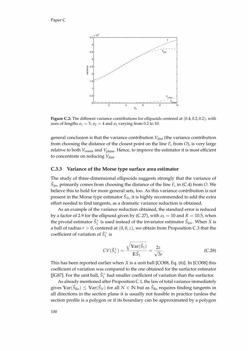
Paper C

2 4 6 8 100

0.5

1

1.5

2

2.5

3

3.5

4

4.5x 10

5

a3

variance

Vdist

Vorient

Vplane

T

Figure C.2: The different variance contributions for ellipsoids centered at (0.4, 0.2, 0.2), withaxes of lengths a1 = 5, a2 = 4 and a3 varying from 0.2 to 10.

general conclusion is that the variance contribution Vdist (the variance contributionfrom choosing the distance of the closest point on the line Fz from O), is very largerelative to both Vorient and Vplane. Hence, to improve the estimator it is most efficientto concentrate on reducing Vdist.

C.3.3 Variance of the Morse type surface area estimator

The study of three-dimensional ellipsoids suggests strongly that the variance ofSinv primarily comes from choosing the distance of the line Fz in (C.4) from O. Webelieve this to hold for more general sets, too. As this variance contribution is notpresent in the Morse type estimator SN , it is highly recommended to add the extraeffort needed to find tangents, as a dramatic variance reduction is obtained.

As an example of the variance reduction obtained, the standard error is reducedby a factor of 2.9 for the ellipsoid given by (C.27), with a3 = 10 and R = 10.5, whenthe pivotal estimator S+

1 is used instead of the invariator estimator Sinv. When X isa ball of radius r > 0, centered at (0, 0, z), we obtain from Proposition C.3 that thecoefficient of variation of S+

1 is

CV(S+1 ) =

√Var(S1)

ES1=

2z√3r

. (C.28)

This has been reported earlier when X is a unit ball [CO08, Eq. (6)]. In [CO08] thiscoefficient of variation was compared to the one obtained for the surfactor estimator[JG87]. For the unit ball, S+

1 had smaller coefficient of variation than the surfactor.As already mentioned after Proposition C.1, the law of total variance immediately

gives Var(Sflo) ≤ Var(SN) for all N ∈ N but as Sflo requires finding tangents inall directions in the section plane it is usually not feasible in practice (unless thesection profile is a polygon or if its boundary can be approximated by a polygon

100

C.3. Variance

using automated segmentation as briefly discussed in Section C.5.2). We thereforerestrict attention to SN in what follows.

Let Y = X ∩ L2, L2 ∈ L2, be the section profile. Applying systematic samplingin the section plane typically reduces the variance. More specifically, using thatM(Y, U) = M(Y, U + π), U ∼ unf(S2 ∩ L2), and Cauchy-Schwarz inequality, weobtain

Var(S2N) ≤ Var(SN) ≤ Var(S1) (C.29)

for all N ∈ N. This was shown for X ∈ K in [DJ13, Section 2.2]. We only mentionhere that using [GACO00, Eq. (2.4)], the variance of the Morse type estimator SN

can be expressed as

Var(SN) = Vplane + E[2π

N

N−1

∑l=0

g(ul πN)−

∫S2∩L2

g(ω)dω | L2

],

where the function g is the circular covariogram of M on the section profile

g(ω) =∫

S2∩L2

M(Y, u)M(Y, u + ω)du, ω ∈ S2 ∩ L2.

C.3.4 Efficiency of the Morse type surface area estimator

We now discuss how the number N of directions in L2 should be chosen so thatthe variance of SN becomes small while still keeping a reasonable workload of thesampling procedure in L2. As the variance contribution Vplane is common for allsurface area estimators considered here, we ignore this contribution in the followingdiscussion and consider the variance of SN given L2. Clearly, the function f (N) =

Var(SN |L2) depends crucially on the shape of the underlying object. We thereforecarried out a simulation study with a variety of different shapes shown in Figure C.3.The simulations were done using R.

Shape 1 Shape 2 Shape 3 Shape 4 Shape 5

Shape 6 Shape 7 Shape 8 Shape 9 Shape 10

Figure C.3: Polygons and half-circles.

101

Paper C

In the next section, we determine the empirical CV’s of SN , N ∈ {1, 2, 3, 4, 5},from independent Monte Carlo replications and derive an empirical recommenda-tion for the choice of N. In Section C.3.4.2 we compare empirically the precision andworkload required for the new estimator SN and the well-known estimator Sgrid.

C.3.4.1 Choice of N

Although the variance of SN for a given section profile does not increase whenthe number of orientations sampled is doubled, as shown in (C.29), it is not a non-increasing function of N. Table C.2 presents estimates of the CV’s for the shapes in

CV N = 1 N = 2 N = 3 N = 4 N = 5

Shape 1 0.6388 0.0242 0.0151 0.0085 0.0055Shape 2 0.3410 0.0848 0.0146 0.0141 0.0123Shape 3 0.2652 0.1048 0.0249 0.0087 0.0120Shape 4 0.2587 0.1487 0.0246 0.0149 0.0090Shape 5 0.1376 0.0188 0.0239 0.0084 0.0049Shape 6 0.1970 0.0228 0.0065 0.0080 0.0029Shape 7 0.2217 0.0747 0.0456 0.0167 0.0072Shape 8 0.3025 0.0422 0.0331 0.0204 0.0082Shape 9 0.2783 0.0129 0.0037 0.0023 0.0013Shape 10 0.2542 0.0908 0.0255 0.0162 0.0091

Table C.2: CV for the shapes in Figure C.3.

Figure C.3, which are all contained in a reference disk of radius one, centered at O. Torecommend a value of N, we suggest that a CV of not more than 2.5% is acceptable.Hence, the smallest N for a given shape where the empirical CV is 2.5% or less,is our recommendation for the choice of N. We only need to find tangents in twodirections for shapes 1, 5, 6 and 9, in three directions for shapes 2, 3 and 4 and in fourdirections for shapes 7, 8 and 10. For all simulated ellipses, two orientations give aCV of less than 2.5%. This is even true for ellipses not containing the reference pointO. This is not surprising as it follows from [DJ13] that S2 and Sflo are identical whenY is an ellipse with O in its interior, as already mentioned at the end of Section C.2.2for three-dimensional ellipsoids. When the reference point is moved away from thecenter of an ellipse, the CV increases. This is evident for a disk from (C.28). Theelongation of the ellipse does not seem to influence the CV when N > 1. For N = 1,the CV increases slightly for increased elongation of the ellipse.

A number of simulations were carried out and they suggest strongly that takingN = 4 is sufficient for obtaining a CV of less than 2.5% for a large class of shapes.Although the CV can increase as N increases, as is the case for Shape 5 with N = 2and N = 3, it is our experience that this increase is rare, and, when it occurs, it is notsubstantial. Therefore taking N = 4 instead of N = 3 should typically not decreasethe precision of the estimator. When the object of interest resembles an ellipse, werecommend using N = 2. We note that these recommendations are only based on

102

C.3. Variance

the variance of the sampling procedure. When there are other sources of variationthat are much larger than the variance due to the sampling procedure, N = 2 istypically adequate, see Section C.4.4.

C.3.4.2 Comparison of SN and Sgrid

We still consider a given section profile Y = X∩ L2 and fix L2 ∈ L2. An alternative tothe Morse type estimator SN is the invariator grid estimator Sgrid given by (C.5). Wecompare the efficiency of these two estimators by finding the amount of workloadneeded to estimate E[Sflo|L2] at a given precision. Define the complexity numbers

CSN= total number of tangents for the N directions,

CSgrid= 2 ∑

zχ(Y ∩ Fz) + ∑

z1{(Y∩Fz)=∅} .

Hence, CSgridis the total number of points in the intersection of the boundary of the

section profile with the test lines plus the number of test lines that do not hit thesection profile. Both complexity numbers are motivated by the number of mouseclicks in an interactive microscopy software to determine the estimator; see alsoSection C.4.3. The workload in obtaining these numbers is typically not equivalent,as determining a critical point is most likely more difficult than to determine if a linehits the boundary of the object or not. But given the ratio Q = CSgrid

/CSN, a clinical

expert can decide if it is more feasible to use SN or Sgrid. The simulation study showsstrong evidence for that SN should be preferred to Sgrid, at least when N > 1.

For a given polygon we generated 1000 independent replications of SN for agiven N and of Sgrid for a given grid distance d. From these observations we calcu-lated an empirical estimate for the variance of SN , Sgrid, respectively, and recordedthe complexity constants CSN

. We then used a normal kernel with smoothness pa-rameter s to smooth Var(Sgrid) as a function of the grid distance d. We denote thesmoothed estimate of the variance by Vars(Sgrid). For a given N we found d suchthat Sgrid has essentially the same precision as SN , that is, such that

|Vars(Sgrid)− Var(SN)| ≤ 10−6.

Given this d we then again generated 1000 independent replications of Sgrid andcalculated CSgrid

. For a given N and the corresponding d we obtained an unbiasedestimate of the ratio Q

Q =1

1000

1000

∑i=1

CSgrid

CSN

.

In Table C.3 results for the shapes in Figure C.3 can be seen, where the smoothnessparameter s = 0.1 has been used. When N > 2, d is close to zero and Q very large(much greater than 100) for all the shapes in Figure C.3. This means that Sgrid onlyattains the efficiency of SN when unrealistically many test lines are used, makingthe complexity number of Sgrid large compared to the one of SN . For ellipses we findthat Q > 2 when N = 1 and that it is very large when N = 2. The ratio Q typicallydecreases with increased elongation of an ellipse.

103

Paper C

Var d Q

Shape 1N = 1 3.52 0.81 2.9N = 2 4.8 · 10−3 ' 0 �100

Shape 2N = 1 6.7 · 10−2 0.64 4.9N = 2 7.2 · 10−3 0.21 22.6

Shape 3N = 1 2.56 · 10−1 0.65 3.7N = 2 3.84 · 10−2 0.32 7.9

Shape 4N = 1 2.08 · 10−1 0.68 4.9N = 2 7.2 · 10−2 0.46 5.3

Shape 5N = 1 1.23 0.48 5.0N = 2 2.08 · 10−2 ' 0 �100

Shape 6N = 1 1.47 0.51 3.2N = 2 1.6 · 10−2 ' 0 �100

Shape 7N = 1 5.92 · 10−1 0.36 8.6N = 2 6.72 · 10−2 0.10 52.1

Shape 8N = 1 1.33 0.58 4.4N = 2 1.34 · 10−2 0.04 �100

Shape 9N = 1 4.06 · 10−1 0.43 10.0N = 2 8.30 · 10−4 ' 0 �100

Shape 10N = 1 4.19 · 10−1 0.40 12.0N = 2 5.41 · 10−2 0.16 35.0

Table C.3: Comparison for the shapes in Figure C.3.

The simulations imply that Q is always greater than 2. Hence, SN should at leastbe preferred to Sgrid if the workload needed to identify a tangent, as well as its typeand critical value, is not more than twice of that needed to determine if a line hitsthe boundary of an object or not. It should be noted that this factor 2 is a worst-casescenario. The ratio Q can be much larger than two even when N = 1, as can be seenin Table C.3. When the software, described in Section C.4.3, is used, the estimator SN

can be obtained very efficiently and should therefore always be preferred to Sgrid.

C.3.4.3 Convex hull

Rather surprisingly it is not necessarily better (with respect to variance) to find SN

for the convex hull of an object than for the true object. We show this by an example.The object in Figure C.4 to the left is a disk of radius r, where one fourth has beencut off, and the one to the right is its convex hull. In Table C.4 estimates for the CV’sbased on 1000 independent replications of SN for N ∈ {1, 2, 3} and each of the twoobjects can be seen.

We note that the CV’s for the convex hull, the object to the right in Figure C.4,are considerably larger than those for the object to the left. This can be explained by

104

C.4. Application of the Morse type surface area estimator

Figure C.4: A disk of radius r, where one fourth has been cut off, and its convex hull.

CV N = 1 N = 2 N = 3

Fig. C.4 left 0.001140 0.000165 0.000357Fig. C.4 right 0.075878 0.040691 0.020190

Table C.4: CV for the objects in Figure C.4

considering the integrand in the generalized flower estimator, the function M. Thetrue value E[Sflo|L2] can be written as

E[Sflo|L2] = 2∫ 2π

0f (α)dα.

where for the object to the left the function f is a constant, f (α) = r2 for all α ∈[0, 2π), while for the convex hull

f (α) =

r2, α ∈ [0, 3π/2)

r2 sin2 α, α ∈ [ 3π2 , 7π

4 )

r2 cos2 α, α ∈ [ 7π4 , 2π).

This explains the greater variance of SN for the convex hull.

C.4 Application of the Morse type surface area estimator togiant-cell glioblastoma

We illustrate the application of the Morse type estimator SN in a study of giant-cellglioblastoma. The goal is to estimate the average surface area of the nucleus of giant-cell glioblastoma from microscopy images. Giant-cell glioblastoma is a rare brainneoplasm which accounts for 1% of glioblastomas. It is formerly known as monstro-cellular brain tumour. Histologically, the tumour is characterized by bizarre-looking,variable sized and shaped multinucleated giant-cells with abundant eosinophilic cy-toplasm [OPN+00]. Giant-cell glioblastoma is a subtype of glioblastoma multiforme,however the rarity of giant-cell glioblastoma has prevented further characterization.Giant-cell glioblastoma is more prevalent in young-male patients and tends to occurmore in parietal and temporal lobe of brain. We chose to illustrate the estimator forthe nuclei of giant-cell glioblastoma as they are typically non-convex in shape, seeFigure C.5.

105

Paper C

Figure C.5: Section profiles through a nucleoli of the nuclei of two giant-cell glioblastoma.

C.4.1 Model-based setting

In the preceding sections we have assumed that the structure of interest is deter-ministic and the section plane is random, that is we have worked in a design-basedsetting. We will now adopt the common model-based approach, where the par-ticles, here nuclei of giant-cell glioblastoma, are random isotropic and the planeis deterministic. This isotropy assumption allows us to avoid a complicated, timeconsuming protocol, where each particle is sectioned physically or optically by anew isotropically generated plane. Hence we assume that the nuclei are realizationsof an ergodic isotropic random process, meaning that nuclei far away from eachother have independent orientations. We then can apply a model-based version ofthe estimator SN . The estimator is identical to the one given by (C.15), but now theparticle X is assumed to be random and the section plane L2 fixed. For all randomnuclei X we assume that ES(X) = S, where the expectation is with respect to therandom particle process and S is the average surface area of the typical particle. S isthe target quantity. The unbiasedness of the model-based version of the estimatorthen follows from the unbiasedness of the design-based estimator and the stronglaw of large numbers.

C.4.2 Materials and preparation methods

From ten small pieces of tissue biopsies sized 1 mm3 to 2 mm3, one piece was ran-domly chosen, embedded in glycol methacrylate (GMA) for preparation of a plasticblock. Two 40 µm-thick plastic sections were serially sectioned on a microtome(HM355, Microm, DMK & Michelsen, Denmark) and stained with hematoxylin andeosin stain for light microscopy. Data-acquisition was performed using a stereo-logical microscopy system (BX-51 microscope, Olympus, Denmark) equipped withthe NewCast Version 4.1 software package (Visiopharm, Hoersholm, Denmark)and mounted with a digital camera (Olympus DP72) on top of the microscopeto project live views of tissue sections on a monitor. The z-axis of the microscopewas monitored with a Heidenhain electronic microcator and the x-y position wasmonitored by motorized stage system (ProscanTM, Prior Scientific Instruments Ltd.,Cambridge, U.K).

106

C.4. Application of the Morse type surface area estimator

The image of the tumour region was captured and delineated by navigator toolof NewCast with 4× objective. An unbiased counting frame (X × Y, 15 × 13 =

195 µm2) was used to sample randomly a total of n = 51 nuclei. The red and green‘rectangle’ on the images in Figure C.6 is a counting frame. The images of nucleiwere captured by optical disector with an oil objective (100×, NA: 1.25).

As already mentioned in Section C.2, any point in the nucleus can serve asreference point as long as it is easily identifiable in any section direction. We chosethe nucleoli in the selected nuclei as reference points. If a nucleus contained severalnucleoli, we chose one out of all the admissible nucleoli (with respect to the countingframe) with uniform probability. In order to decrease the variance of the estimatorsystematic sampling was applied in the tissue by using a counting frame with astep-length of 400 µm in both x and y direction. This assures that the nuclei can beassumed to have independent orientations. In other words, we can assume thatthe n sampled nuclei are realizations of independent, isotropic random particlesX1, X2, . . . , Xn satisfying ES(Xi) = S for i = 1, . . . , n.

C.4.3 Implementation of the Morse type surface area estimator

The estimator SN was used to estimate the surface areas of the sampled nuclei. InSection C.3.4.1 we recommended to use N = 4, that is to find tangents for four direc-tions in the section plane (N = 2 when the object of interest resembles an ellipsoid),to obtain a good precision of the surface area. In the present implementation weused one, two and four directions in the section plane in order to be able to comparethe performance of the estimators. The estimation was done using an expert-assistedprocedure which was implemented using Matlab. It is based on a program derivedin [Kal12] for estimating the perimeter of planar geometric structures. The interac-tive software is available at the home page home.imf.au.dk/olofth. We give a briefdescription of it in the following.

The present implementation is an off-line expert-assisted procedure, where thesampled section profiles – microscopy images in JPEG format – are used as input.The user, preferably a clinical expert, can choose the number N of directions thatare to be sampled. As previously stated we recommend using N = 4 (N = 2 forellipsoids) but we describe the procedure for an arbitrary N. Microscopy images areoften stored with a scale, see for instance Figure C.5 to the left. If this is the case, theuser should indicate the scale before running the procedure. If a scale is reported,the calculated surface area estimate is given on this scale, otherwise it is given inpixel units. We assume in the following that a scale is given.

When the procedure is run, the image pops up with a short explanation of whatthe user should do next. The measurement procedure consists of three steps whichare illustrated in Figure C.6.

Scale The user left clicks on the endpoints of the scale, see the image in the upperleft corner in Figure C.6. This tells the program that the length of the red‘measure’ line segment is 10.706 µm.

107

Paper C

Figure C.6: An illustration of the expert-assisted procedure on one section profile through anucleolus of the nucleus of a giant-cell glioblastoma. The short black line segment indicatesthe sampled direction. Positive tangents are colored red while negative tangents are coloredblue.

Reference point The user left clicks on the reference point, see the image in theupper right corner in Figure C.6.

Tangents The computer generates a random unit vector U in the section planeincluding an angle α0 with the x-axis that is uniform in [0, π/N). In the imagein the lower left corner in Figure C.6, this vector is indicated as a short blackline segment attached to the red line orthogonal to U, passing through theposition of the mouse cursor. The line can be translated using the mouse.The user now marks all tangent positions of this line to the section profile,clicking left whenever a positive tangent is located, and clicking right forevery negative tangent. If N > 1 this step is repeated with all N − 1 lines withassociated angles α0 + lπ/N, l ∈ {1, 2, . . . , N − 1}.

When these three steps are completed and the user has found all tangents for theN sampled directions an estimate SN of the surface area is calculated. The numberof tangents that need to be placed gives the complexity number CSN

defined in

108

C.4. Application of the Morse type surface area estimator

Section C.3.4.2. It should be noted again that it certainly is more time consumingto place tangents at a given direction than just counting intersection points of theprofile boundary with a given line, as is the case for the invariator estimator. But foran experienced user of the software, the Morse type estimator SN can be obtainedvery efficiently and should be preferred to the alternative invariator grid estimatorSgrid.

As biological images are blurred, there might be tangents that appear to passthrough a point of inflection of the boundary (although this event has probabilityzero with idealized mathematical particles). The easiest solution is to ignore thesetangent lines, and neither left- nor right click at these positions. This is in corre-spondence with the theory, as a sweeping line passing through this tangent willneither increase nor decrease the associated Euler characteristic. It can also happenin practice, that the sweeping line appears to be tangent to the section profile atmore than one point for certain critical values. As the images are blurred, it couldfor example appear that the sweeping line enters more than one new connectedcomponent at a critical value or that it enters a new connected component andleaves a part of the section profile at the same critical value. These events also haveprobability zero with idealized mathematical particles. To deal with these tangents,we simply suggest making a left- or a right mouse click for every change, withouttranslating the line.

C.4.4 Results

We used the expert-assisted procedure to obtain estimates of the surface area of then = 51 section profiles. We did this for N = 1, 2 and 4. An unbiased estimator forthe average surface area of the nucleus X of a giant-cell glioblastoma is then givenby

SaveN (X) =

151

51

∑i=1

SN(Xi ∩ L2),

where L2 is a fixed plane and SN is the Morse-type estimator given by (C.15). Empir-ical estimates for the average surface areas can be found in Table C.5.

N = 1 N = 2 N = 4

SaveN (X) 675.0 µm2 597.8 µm2 599.3 µm2

Table C.5: Empirical estimates for the average surface area of the nucleus of a giant-cellglioblastoma, depending on the number N of systematic directions used in the section plane.

In Figure C.7 boxplots for the surface area estimates of the nuclei for N = 1, 2and 4, respectively, can be found. The red lines in Figure C.7 are the medians, thebottom and the top of the boxes represent the lower quartiles (25th percentiles) andthe upper quartiles (75th percentiles), respectively, and the red ‘pluses’ are outliers(more than 1.5 IQR from the upper quartiles). The boxplots in Figure C.7 do notsuggest that sampling with a higher number N of directions gives a more precise

109

Paper C

0

500

1000

1500

2000

2500

3000

1 2 4

Figure C.7: Boxplots for the surface area estimates of the 51 nuclei for N = 1, 2 and 4,respectively.

estimator. This seemingly counter-intuitive result can be explained by looking at thedifferent sources of variation of Save

N (X). The variance of SaveN (X) can be decomposed

into the true population variance, that is the variation in surface area among thenuclei, and the mean variance due to the estimation procedure within each nucleus.The variance due to the estimation procedure within each nucleus can then again bedecomposed into Vplane and Vorient, as shown in Proposition C.1. The true populationvariance is unknown and as the data only consist of one section profile for eachsampled nuclei we can not assess Vplane. For a given nucleus, Vorient can be estimatedfrom the section profile. This was done for each of the estimators in Table C.5 fora few of the section profiles. A large decrease in Vorient was observed for each ofthe studied nuclei when N was increased. This decrease in Vorient was much morepronounced when N was increased from one to two than when it was increasedfrom two to four. However, this variance contribution is very small compared tothe sum of the true population variance and the mean variance due to choosing theplane within each nucleus. This explains why there is no noticeable precision gainin Figure C.7 when N is increased. In the present application the choice N = 1 led toan extreme outlier and Vorient that is much larger than when N = 2. As a conclusion,this example suggests that the choice N = 2 is preferrable in situations where arelatively large population variance is present. The workload for the choice N = 2is not very high.

110

C.5. Discussion

C.5 Discussion

C.5.1 Account of main results

We have presented the Morse type surface area estimator and an expert-assistedprotocol to apply it in practice. The Morse type estimator is a generalization ofCruz-Orive’s surface area estimator for convex objects [CO05, Eq. (3.2)] ((C.16) withN = 2) to non-convex objects.

The surfactor is an alternative surface area estimator. The surfactor does not onlyrequire measuring distances in an IR section plane but also angles of the sectionprofile with certain test rays. It was implied in [CO05] that this requirement toperform angle measurements might be difficult in practice and yield inaccurateestimates due to the singularity in its representation. In light of this belief and thesimplicity of the estimator (C.16) it was claimed in [CO05] that (C.16) was the onlyreasonably efficient surface area estimator available at that time.

As mentioned in Section C.3.3, the surfactor was compared to the one-ray pivotalestimator, (C.17) with N = 1, in [CO08]. This variance comparison was extended toellipsoidal particles in [DJ13]. The results obtained in [DJ13] show that the surfactorperforms better than previously thought. In a simulation study involving ellipsoids,the surfactor was shown to be neither much affected by the singularity in its repre-sentation nor by inaccuracies in the necessary angle measurements. In [DJ13] it wasalso shown that the surfactor with two orthogonal directions sampled in the sectionplane [DJ13, Eq. (12) with N = 4] needs twice as much workload to obtain similarprecision as (C.16) with N = 2. Hence, although the surfactor is a better competitorto (C.16) than previously expected, (C.16) is more efficient and should be preferredwhen the object of interest is convex. This recommendation can be transferred tothe Morse type surface area estimator, which we showed to be the preferred surfacearea estimator available.

We have shown in Section C.3.1 that the variance of the pivotal estimator Spiv

decomposes into three parts Vplane, Vorient and Vdist according to the randomizationof the section plane, and the orientation and position of the test line, respectively.Among all estimators considered in the present paper, the generalized flower es-timator has the lowest variance, as this variance coincides with Vplane. However,this estimator requires exact knowledge of the boundary of the section profile. Wetherefore also considered estimators derived from Sinv that still have a reasonableworkload but a better variance than Sinv. The detailed analysis of the three variancecontributions in Section C.3.2 in the case of ellipsoidal particles showed that Vdist

is by far the largest variance contribution. We therefore suggested the Morse typesurface area estimator SN for which this variance contribution vanishes. By choosingthe number N of systematic random test directions, also the variance contributiondue to the randomization of the direction can be decreased. However, we have seenthat only small values of N have to be considered, and that values N = 2 or N = 4are theoretically advisable depending on the regularity of the objects. This also isin agreement with Figure C.2 that shows that Vorient is a relatively small variance

111

Paper C

contribution (in the case of ellipsoids).The application example of giant-cell glioblastoma showed that other sources

of variation, such as the population variance or the uncertainty of measurementsdue to blurred or ambiguous images can be of the same order or larger than thetheoretical variance contribution of the estimator. This indicates that the choiceN = 2 appears to be appropriate in real-world applications.

C.5.2 Automatic and semi-automatic estimation of surface area

Inspired by [CO12] it was shown in [TK13] that the generalized flower estimatorSflo given by (C.12) and the integrated surfactor [CO12, Eq. (24)] coincide. The gen-eralized flower estimator is the optimal estimator with respect to variance (amongall the estimators considered in this paper) but as mentioned in Section C.3.3 it cantypically not be calculated in practice if the section profile is not a polygon. However,if it is possible to identify the boundary of a given section profile by automatedsegmentation, the boundary can be approximated by a polygon. Using this approxi-mation the generalized flower estimator Sflo, with the true section profile Y = X ∩ L2

replaced by its estimate, can be obtained using [TK13, Corollary 10] as mentioned inSection C.2.2.3. If the segmentation is flawless, this automatic estimator is unbiased.However, if it is of poor quality, the estimator can be heavily biased. To deal withthis problem a semi-automatic procedure for estimating surface area was proposedin [DJ13], based on a similar approach for volume estimation in [HNAJ11]. In thesemi-automatic procedure, a clinical expert supervises the process and determines ifthe automated segmentation of the boundary of a given section profile is satisfactoryor not. If it is determined to be satisfactory the surface area is obtained using Sflo

with Y being the estimate obtained by the automated segmentation. If it is unsatisfac-tory, the clinical expert intervenes and performs the necessary measurements in thesection plane. In [DJ13] it was suggested to use (C.16) in the case where all particlesare convex. We suggest to use the Morse-type estimator, which does not requireany convexity assumption and reduces to (C.16) when the particles are convex. Thissemi-automatic procedure can reduce the workload substantially.

Acknowledgement

This research was supported by Centre for Stochastic Geometry and AdvancedBioimaging, funded by the Villum Foundation. The authors want to thank BenedicteParm Ulhøi at the Institute of Pathology, Aarhus University Hospital NBG, for pro-viding the tissue biopsies and expert knowledge on histological aspects of tumours.The authors also want to thank Thomas Kallemose for writing the program whichthe expert-assisted procedure is based on.

112

Appendix: Variance decomposition for ellipsoids

Appendix: Variance decomposition for ellipsoids

The following proposition gives the different variance contributions in Proposi-tion C.1 more explicitly when X is a three-dimensional ellipsoid containing O. Aproof can be found in [Thó10, Theorem 25]. As the reference set RB3 is triviallyinvariant under all rotations at the origin, and as the sampling procedure is rotationinvariant, we may assume without loss of generality that the ellipsoid’s main axesare parallel to the standard coordinate axes.

Proposition C.4. Let E3 ⊆ RB3 be a non-degenerate ellipsoid given by

E3 ={

x ∈ R3∣∣∣ 3

∑i=1

(xi − zi

ai

)2

≤ 1}

, (C.30)

where a1, a2, a3 > 0 and (z1, z2, z3) ∈ R3. If O ∈ E3, the variance of Sinv given by (C.4),can be expressed as

Var(Sinv) = Vdist + Vorient + Vplane,

where

Vdist = 4π∫ 2π

0

∫ π/2

0

(R2( 1

λ1+

1λ2

+ (z′1)2 + (z′2)

2)−( 3

4λ21+

12λ1λ2

+3

4λ22

+34((z′1)

4 + 2(z′1)2(z′2)

2 + (z′2)4) + ((z′1)u

′1 + (z′2)u

′2)

2(9

21

λ1+

32

1λ2

)+ (z′1u′′1 + z′2u′′2 )

2( 3

2λ1+

92λ2

)))sin θdθdφ, (C.31)

Vorient = 4π∫ 2π

0

∫ π/2

0

( 34λ2

1+

12λ1λ2

+3

4λ22+

34((z′1)

4 + 2(z′1)2(z′2)

2 + (z′2)4)

+ (z′1u′1 + z2u′2)2( 9

2λ1+

32λ2

)+ (z′1u′′1 + z′2u′′2 )

2( 3

2λ1+

92λ2

)− 1

2

( 1λ1

+1

λ2+ (z′1)

2 + (z′2)2)2)

sin θdθdφ, (C.32)

Vplane = 2π∫ 2π

0

∫ π/2

0

( 1λ1

+1

λ2+ (z′1)

2 + (z′2)2)2

sin θdθdφ

−( ∫ 2π

0

∫ π/2

0

( 1λ1

+1

λ2+ (z′1)

2 + (z′2)2)

sin θdθdφ)2

. (C.33)

Here λ−1/21 and λ−1/2

2 are the lengths of the semiaxes of the ellipse E3 ∩ L2, u′ = (u′1, u′2)t,

u′′ = (u′′1 , u′′2 )t its corresponding principal axes and (z′1, z′2)

t its center, all written withrespect to a suitably chosen orthonormal basis of the IR plane L2.

Although the decomposition formulae for ellipsoids are quite complicated it is notdifficult to derive a theoretical formula for the total variance of Sinv when X is an

113

Paper C

ellipsoid. When X is a convex body, χ(X ∩ L2 ∩ Fz) is a Bernoulli random variableand hence using the unbiasedness of Sinv

Var(Sinv) = S(∂X)(S(∂(RB3))− S(∂X)). (C.34)

As a side note, this immediately gives the coefficient of variation of the estimator,which is

CV(Sinv) =( 4πR2

S(∂X)− 1)1/2

,

in accordance to [CO08, Eq. (18)], as well as the total variance (C.26) of the estimatorwhen X is a ball.

Let now E3 be a non-degenerate ellipsoid given by (C.30). Assume without lossof generality that a1 ≥ a2 ≥ a3. Then the surface area of E3 is given by [Eag58,(12) on p. 281]

S(∂E3) = 2π(

a23 +

a2a23√

a21 − a2

3

F(σ, m) + a2

√a2

1 − a23E(σ, m)

),

where

σ = arcsin

√a2

1 − a23

a21

, m =a2

1(a22 − a2

3)

a22(a2

1 − a23)

and F(·, ·) and E(·, ·) are the incomplete elliptic integrals of the first kind and of thesecond kind, respectively. Inserting this into (C.34), we find

Var(Sinv) = 4π2(

2R2(

a23 +

a2a23√

a21 − a2

3

F(σ, m) + a2

√a2

1 − a23E(σ, m)

)

−((

a23 +

a2a23√

a21 − a2

3

F(σ, m) + a2

√a2

1 − a23E(σ, m)

))2). (C.35)

For an oblate ellipsoid (that is when a1 = a2 > a3), the surface area has an explicitform and the total variance becomes

Var(Sinv) = 4π2(

2R2(

a21 +

a1a23√

a21−a2

3log(√

a21−a2

3+a1a3

))−(

a21 +

a1a23√

a21−a2

3log(√

a21−a2

3+a1a3

))2);

see [Thó10, p. 34] for a derivation. When X is an oblate or a prolate ellipsoid, explicitanalytic expressions for Vplane can be found in [DJ13, Eq. (2.5) and (2.6)].

Bibliography

[Bad84] A.J. Baddeley. Stochastic geometry and image analysis. In Proceed-ings of the CWI symposium on mathematics and computer science. CWIMonographs, 1984.

114

Bibliography

[BS12] C.G. Bowsher and P.S. Swain. Identifying sources of variation andthe flow of information in biochemical networks. Proceedings of theNational Academy of Sciences, 109(20):E1320–E1328, 2012.

[CO05] L.M. Cruz-Orive. A new stereological principle for test lines in three-dimensional space. J. Microsc., 219(1):18–28, 2005.

[CO08] L.M. Cruz-Orive. Comparative precision of the pivotal estimators ofparticle size. Image Anal. Stereol., 27(1):17–22, 2008.

[CO11] L.M. Cruz-Orive. Flowers and wedges for the stereology of particles.J. Microsc., 243(1):86–102, 2011.

[CO12] L.M. Cruz-Orive. Uniqueness properties of the invariator, leading tosimple computations. Image Anal. Stereol., 31(2):89–98, 2012.

[CORHAP10] L.M. Cruz-Orive, M.L. Ramos-Herrera, and E. Artacho-Pérula. Stereo-logy of isolated objects with the invariator. J. Microsc., 240(2):94–110,2010.

[DeH67] R.T. DeHoff. The quantitative estimation of mean surface curvature.Trans. Metal. Soc. AIME, 239:617–621, 1967.

[DJ13] J. Dvorák and E.B.V. Jensen. On semiautomatic estimation of surfacearea. J. Microsc., 250(2):142–157, 2013.

[Eag58] A. Eagle. The Elliptic Functions as they should be: An account, withapplications, of the functions in a new canonical form. Galloway andPorter, Cambridge, 1958.

[GACO00] X. Gual-Arnau and L.M. Cruz-Orive. Systematic sampling on thecircle and on the sphere. Adv. Appl. Prob., 32(3):628–647, 2000.

[Gun88] H.J.G. Gundersen. The nucleator. J. Microsc., 151(1):3–21, 1988.

[HNAJ11] L.V. Hansen, J.R. Nyengaard, J.B. Andersen, and E.B.V. Jensen. Thesemi-automatic nucleator. J. Microsc., 242(2):206–215, 2011.

[Jen98] E.B.V. Jensen. Local Stereology. World Scientific, Singapore, 1998.

[JG87] E.B.V. Jensen and H.J.G. Gundersen. Stereological estimation ofsurface area of arbitrary particles. Acta Stereol., 6:25–30, 1987.

[Kal12] T. Kallemose. Application of stereological projection formulae forperimeter estimation. Master’s thesis, Aarhus University, 2012.

[Mil63] J.W. Milnor. Morse Theory. Princeton University Press, Princeton,1963.

[OPN+00] H. Ohgaki, A. Peraud, Y. Nakazato, K. Watanabe, and A. Von Deim-ling. Giant cell glioblastoma. In World Health Organization classificationof tumours. Pathology and genetics of tumours of the nervous system, pages40–41. IARC Press, Lyon, 2000.

[Thó10] Ó. Thórisdóttir. Variance for surface area estimation based on theinvariator. Master’s thesis, Aarhus University, 2010.

115

Paper C

[TK13] Ó. Thórisdóttir and M. Kiderlen. The invariator principle in convexgeometry. Submitted, 2013.

116