Advances in Computer Vision and Pattern Recognitionvplab/downloads/opt/(Advances in Computer... ·...

Advances in Computer Vision and Pattern Recognition

Optimization for Computer Vision

Marco Alexander Treiber

An Introduction to Core Concepts and Methods

Advances in Computer Vision and PatternRecognition

For further volumes:

http://www.springer.com/series/4205

Marco Alexander Treiber

Optimization for ComputerVision

An Introduction to Core Conceptsand Methods

Marco Alexander TreiberASM Assembly Systems GmbH & Co. KGMunich, Germany

ISSN 2191-6586 ISSN 2191-6594 (electronic)Advances in Computer Vision and Pattern RecognitionISBN 978-1-4471-5282-8 ISBN 978-1-4471-5283-5 (eBook)DOI 10.1007/978-1-4471-5283-5Springer London Heidelberg New York Dordrecht

Library of Congress Control Number: 2013943987

© Springer-Verlag London 2013This work is subject to copyright. All rights are reserved by the Publisher, whether the whole or partof the material is concerned, specifically the rights of translation, reprinting, reuse of illustrations,recitation, broadcasting, reproduction on microfilms or in any other physical way, and transmission orinformation storage and retrieval, electronic adaptation, computer software, or by similar or dissimilarmethodology now known or hereafter developed. Exempted from this legal reservation are brief excerptsin connection with reviews or scholarly analysis or material supplied specifically for the purpose of beingentered and executed on a computer system, for exclusive use by the purchaser of the work. Duplicationof this publication or parts thereof is permitted only under the provisions of the Copyright Law of thePublisher’s location, in its current version, and permission for use must always be obtained fromSpringer. Permissions for use may be obtained through RightsLink at the Copyright Clearance Center.Violations are liable to prosecution under the respective Copyright Law.The use of general descriptive names, registered names, trademarks, service marks, etc. in thispublication does not imply, even in the absence of a specific statement, that such names are exemptfrom the relevant protective laws and regulations and therefore free for general use.While the advice and information in this book are believed to be true and accurate at the date ofpublication, neither the authors nor the editors nor the publisher can accept any legal responsibility forany errors or omissions that may be made. The publisher makes no warranty, express or implied, withrespect to the material contained herein.

Printed on acid-free paper

Springer is part of Springer Science+Business Media (www.springer.com)

Series EditorsProf. Sameer Singh

Research School of Informatics

Loughborough University

Loughborough

UK

Dr. Sing Bing Kang

Microsoft Research

Microsoft Corporation

Redmond, WA

USA

This book is dedicated to my family:My parents Maria and ArminMy wife BirgitMy children Lilian and MarisaI will always carry you in my heart

Preface

In parallel to the much-quoted enduring increase of processing power, we can

notice that that the effectiveness of the computer vision algorithms themselves is

enhanced steadily. As a consequence, more and more real-world problems can be

tackled by computer vision. Apart from their traditional utilization in industrial

applications, progress in the field of object recognition and tracking, 3D scene

reconstruction, biometrics, etc. leads to a wide-spread usage of computer vision

algorithms in applications such as access control, surveillance systems, advanced

driver assistance systems, or virtual reality systems, just to name a few.

If someone wants to study this exciting and rapidly developing field of computer

vision, he or she probably will observe that many publications primarily focus on

the vision algorithms themselves, i.e. their main ideas, their derivation, their

performance compared to alternative approaches, and so on.

Compared to that, many contributions place less weight on the rather “technical”

issue of the methods of optimization these algorithms employ. However, this does

not come up to the actual importance optimization plays in the field of computer

vision. First, the vast majority of computer vision algorithms utilize some form of

optimization scheme as the task often is to find a solution which is “best” in some

respect. Second, the choice of the optimization method seriously affects the perfor-

mance of the overall method, in terms of accuracy/quality of the solution as well as

in terms of runtime. Reason enough for taking a closer look at the field of

optimization.

This book is intended for persons being about to familiarize themselves with the

field of computer vision as well as for practitioners seeking for knowledge how to

implement a certain method. With existing literature, I feel that there are the

following shortcomings for those groups of persons:

• The original articles of the computer vision algorithms themselves often don’t

spend much room on the kind of optimization scheme they employ (as it is

assumed that readers already are familiar with it) and often confine themselves at

reporting the impact of optimization on the performance.

vii

• General-purpose optimization books give a good overview, but of course lack in

relation to computer vision and its specific requirements.

• Dedicated literature dealing with optimization methods used in computer vision

often focusses on a specific topic, like graph cuts, etc.

In contrast to that, this book aims at

• Giving a comprehensive overview of a large variety of topics of relevance in

computer vision-related optimization. The included material ranges from classi-

cal iterative multidimensional optimization to up-to-date topics like graph cuts

or GPU-suited total variation-based optimization.

• Bridging the gap between the computer vision applications and the optimization

methods being employed.

• Facilitating understanding by focusing on the main ideas and giving (hopefully)

clearly written and easy to follow explanations.

• Supplying detailed information how to implement a certain method, such as

pseudocode implementations, which are included for most of the methods.

As the main purpose of this book is to introduce into the field of optimization, the

content is roughly structured according to a classification of optimization methods

(i.e. continuous, variational, and discrete optimization). In order to intensify the

understanding of these methods, one or more important example applications in

computer vision are presented directly after the corresponding optimization

method, such that the reader can immediately learn more about the utilization of

the optimization method at hand in computer vision. As a side effect, the reader is

introduced into many methods and concepts commonly used in computer vision

as well.

Besides hopefully giving easy to follow explanations, the understanding is

intended to be facilitated by regarding each method from multiple points of view.

Flowcharts should help to get an overview of the proceeding at a coarse level,

whereas pseudocode implementations ought to give more detailed insights. Please

note, however, that both of them might slightly deviate from the actual implemen-

tation of a method in some details for clarity reasons.

To my best knowledge, there does not exist an alternative publication which

unifies all of these points. With this material at hand, the interested reader hopefully

finds easy to follow information in order to enlarge his knowledge and develop a

solid basis of understanding of the field.

Dachau Marco Alexander Treiber

March 2013

viii Preface

Contents

1 Introduction . . . . . . . . . . . . . . . . . . . . . . . . . . . . . . . . . . . . . . . . . . . 1

1.1 Characteristics of Optimization Problems . . . . . . . . . . . . . . . . . . 1

1.2 Categorization of Optimization Problems . . . . . . . . . . . . . . . . . . . 3

1.2.1 Continuous Optimization . . . . . . . . . . . . . . . . . . . . . . . . . 4

1.2.2 Discrete Optimization . . . . . . . . . . . . . . . . . . . . . . . . . . . 5

1.2.3 Combinatorial Optimization . . . . . . . . . . . . . . . . . . . . . . . 5

1.2.4 Variational Optimization . . . . . . . . . . . . . . . . . . . . . . . . . 6

1.3 Common Optimization Concepts in Computer Vision . . . . . . . . . . 7

1.3.1 Energy Minimization . . . . . . . . . . . . . . . . . . . . . . . . . . . . 8

1.3.2 Graphs . . . . . . . . . . . . . . . . . . . . . . . . . . . . . . . . . . . . . . 10

1.3.3 Markov Random Fields . . . . . . . . . . . . . . . . . . . . . . . . . . 12

References . . . . . . . . . . . . . . . . . . . . . . . . . . . . . . . . . . . . . . . . . . . . . 16

2 Continuous Optimization . . . . . . . . . . . . . . . . . . . . . . . . . . . . . . . . . 17

2.1 Regression . . . . . . . . . . . . . . . . . . . . . . . . . . . . . . . . . . . . . . . . . 18

2.1.1 General Concept . . . . . . . . . . . . . . . . . . . . . . . . . . . . . . . 18

2.1.2 Example: Shading Correction . . . . . . . . . . . . . . . . . . . . . . 19

2.2 Iterative Multidimensional Optimization: General Proceeding . . . . 22

2.2.1 One-Dimensional Optimization Along a Search

Direction . . . . . . . . . . . . . . . . . . . . . . . . . . . . . . . . . . . . . 25

2.2.2 Calculation of the Search Direction . . . . . . . . . . . . . . . . . 30

2.3 Second-Order Optimization . . . . . . . . . . . . . . . . . . . . . . . . . . . . . 31

2.3.1 Newton’s Method . . . . . . . . . . . . . . . . . . . . . . . . . . . . . . 31

2.3.2 Gauss-Newton and Levenberg-Marquardt Algorithm . . . . . 33

2.4 Zero-Order Optimization: Powell’s Method . . . . . . . . . . . . . . . . . 40

2.4.1 General Proceeding . . . . . . . . . . . . . . . . . . . . . . . . . . . . . 40

2.4.2 Application Example: Camera Calibration . . . . . . . . . . . . 45

2.5 First-Order Optimization . . . . . . . . . . . . . . . . . . . . . . . . . . . . . . . 49

2.5.1 Conjugate Gradient Method . . . . . . . . . . . . . . . . . . . . . . . 50

2.5.2 Application Example: Ball Inspection . . . . . . . . . . . . . . . . 52

2.5.3 Stochastic Steepest Descent and Simulated Annealing . . . . 55

ix

2.6 Constrained Optimization . . . . . . . . . . . . . . . . . . . . . . . . . . . . . . 61

References . . . . . . . . . . . . . . . . . . . . . . . . . . . . . . . . . . . . . . . . . . . . . 64

3 Linear Programming and the Simplex Method . . . . . . . . . . . . . . . . . 67

3.1 Linear Programming (LP) . . . . . . . . . . . . . . . . . . . . . . . . . . . . . . 67

3.2 Simplex Method . . . . . . . . . . . . . . . . . . . . . . . . . . . . . . . . . . . . . 71

3.3 Example: Stereo Matching . . . . . . . . . . . . . . . . . . . . . . . . . . . . . 80

References . . . . . . . . . . . . . . . . . . . . . . . . . . . . . . . . . . . . . . . . . . . . . 85

4 Variational Methods . . . . . . . . . . . . . . . . . . . . . . . . . . . . . . . . . . . . . 87

4.1 Introduction . . . . . . . . . . . . . . . . . . . . . . . . . . . . . . . . . . . . . . . . 87

4.1.1 Functionals and Their Minimization . . . . . . . . . . . . . . . . . 87

4.1.2 Energy Functionals and Their Utilization

in Computer Vision . . . . . . . . . . . . . . . . . . . . . . . . . . . . . 91

4.2 Tikhonov Regularization . . . . . . . . . . . . . . . . . . . . . . . . . . . . . . . 93

4.3 Total Variation (TV) . . . . . . . . . . . . . . . . . . . . . . . . . . . . . . . . . 97

4.3.1 The Rudin-Osher-Fatemi (ROF) Model . . . . . . . . . . . . . . 97

4.3.2 Numerical Solution of the ROF Model . . . . . . . . . . . . . . . 98

4.3.3 Efficient Implementation of TV Methods . . . . . . . . . . . . . 103

4.3.4 Application: Optical Flow Estimation . . . . . . . . . . . . . . . . 104

4.4 MAP Image Deconvolution in a Variational Context . . . . . . . . . . 109

4.4.1 Relation Between MAP Deconvolution

and Variational Regularization . . . . . . . . . . . . . . . . . . . . . 109

4.4.2 Separate Estimation of Blur Kernel

and Non-blind Deconvolution . . . . . . . . . . . . . . . . . . . . . 110

4.4.3 Variants of the Proceeding . . . . . . . . . . . . . . . . . . . . . . . . 113

4.5 Active Contours (Snakes) . . . . . . . . . . . . . . . . . . . . . . . . . . . . . . 116

4.5.1 Standard Snake . . . . . . . . . . . . . . . . . . . . . . . . . . . . . . . . 118

4.5.2 Gradient Vector Flow (GVF) Snake . . . . . . . . . . . . . . . . . 123

References . . . . . . . . . . . . . . . . . . . . . . . . . . . . . . . . . . . . . . . . . . . . . 126

5 Correspondence Problems . . . . . . . . . . . . . . . . . . . . . . . . . . . . . . . . 129

5.1 Applications . . . . . . . . . . . . . . . . . . . . . . . . . . . . . . . . . . . . . . . . 129

5.2 Heuristic: Search Tree . . . . . . . . . . . . . . . . . . . . . . . . . . . . . . . . 133

5.2.1 Main Idea . . . . . . . . . . . . . . . . . . . . . . . . . . . . . . . . . . . . 133

5.2.2 Recognition Phase . . . . . . . . . . . . . . . . . . . . . . . . . . . . . . 134

5.2.3 Example . . . . . . . . . . . . . . . . . . . . . . . . . . . . . . . . . . . . . 140

5.3 Iterative Closest Point (ICP) . . . . . . . . . . . . . . . . . . . . . . . . . . . . 140

5.3.1 Standard Scheme . . . . . . . . . . . . . . . . . . . . . . . . . . . . . . . 140

5.3.2 Example: Robust Registration . . . . . . . . . . . . . . . . . . . . . 143

5.4 Random Sample Consensus (RANSAC) . . . . . . . . . . . . . . . . . . . 149

5.5 Spectral Methods . . . . . . . . . . . . . . . . . . . . . . . . . . . . . . . . . . . . 154

5.5.1 Spectral Graph Matching . . . . . . . . . . . . . . . . . . . . . . . . . 154

5.5.2 Spectral Embedding . . . . . . . . . . . . . . . . . . . . . . . . . . . . . 160

x Contents

5.6 Assignment Problem/Bipartite Graph Matching . . . . . . . . . . . . . . 161

5.6.1 The Hungarian Algorithm . . . . . . . . . . . . . . . . . . . . . . . . 162

5.6.2 Example: Shape Contexts . . . . . . . . . . . . . . . . . . . . . . . . 170

References . . . . . . . . . . . . . . . . . . . . . . . . . . . . . . . . . . . . . . . . . . . . . 174

6 Graph Cuts . . . . . . . . . . . . . . . . . . . . . . . . . . . . . . . . . . . . . . . . . . . . 177

6.1 Binary Optimization with Graph Cuts . . . . . . . . . . . . . . . . . . . . . 177

6.1.1 Problem Formulation . . . . . . . . . . . . . . . . . . . . . . . . . . . . 177

6.1.2 The Maximum Flow Algorithm . . . . . . . . . . . . . . . . . . . . 180

6.1.3 Example: Interactive Object Segmentation/GrabCut . . . . . 185

6.1.4 Example: Automatic Segmentation for Object

Recognition . . . . . . . . . . . . . . . . . . . . . . . . . . . . . . . . . . 191

6.1.5 Restriction of Energy Functions . . . . . . . . . . . . . . . . . . . . 194

6.2 Extension to the Multi-label Case . . . . . . . . . . . . . . . . . . . . . . . . 196

6.2.1 Exact Solution: Linearly Ordered Labeling Problems . . . . 196

6.2.2 Iterative Approximation Solutions . . . . . . . . . . . . . . . . . . 202

6.3 Normalized Cuts . . . . . . . . . . . . . . . . . . . . . . . . . . . . . . . . . . . . 212

References . . . . . . . . . . . . . . . . . . . . . . . . . . . . . . . . . . . . . . . . . . . . . 220

7 Dynamic Programming (DP) . . . . . . . . . . . . . . . . . . . . . . . . . . . . . . 221

7.1 Shortest Paths . . . . . . . . . . . . . . . . . . . . . . . . . . . . . . . . . . . . . . 222

7.1.1 Dijkstra’s Algorithm . . . . . . . . . . . . . . . . . . . . . . . . . . . . 222

7.1.2 Example: Intelligent Scissors . . . . . . . . . . . . . . . . . . . . . . 228

7.2 Dynamic Programming Along a Sequence . . . . . . . . . . . . . . . . . . 232


7.2.2 Application: Active Contour Models . . . . . . . . . . . . . . . . 235

7.3 Dynamic Programming Along a Tree . . . . . . . . . . . . . . . . . . . . . 240


7.3.2 Example: Pictorial Structures for Object Recognition . . . . 243

References . . . . . . . . . . . . . . . . . . . . . . . . . . . . . . . . . . . . . . . . . . . . . 254

Index . . . . . . . . . . . . . . . . . . . . . . . . . . . . . . . . . . . . . . . . . . . . . . . . . . . 255

Contents xi

Chapter 1

Introduction

Abstract The vast majority of computer vision algorithms use some form of

optimization, as they intend to find some solution which is “best” according to

some criterion. Consequently, the field of optimization is worth studying for

everyone being seriously interested in computer vision. In this chapter, some

expressions being of widespread use in literature dealing with optimization are

clarified first. Furthermore, a classification framework is presented, which intends

to categorize optimization methods into the four categories continuous, discrete,

combinatorial, and variational, according to the nature of the set from which they

select their solution. This categorization helps to obtain an overview of the topic

and serves as a basis for the structure of the remaining chapters at the same time.

Additionally, some concepts being quite common in optimization and therefore

being used in diverse applications are presented. Especially to mention are

so-called energy functionals measuring the quality of a particular solution by

calculating a quantity called “energy”, graphs, and last but not least Markov

Random Fields.

1.1 Characteristics of Optimization Problems

Optimization plays an important role in computer vision, because many computer

vision algorithms employ an optimization step at some point of their proceeding.

Before taking a closer look at the diverse optimization methods and their utilization

in computer vision, let’s first clarify the concept of optimization. Intuitively, in

optimization we have to find a solution for a given problem which is “best” in the

sense of a certain criterion.

Consider a satnav system, for example: here the satnav has to find the “best”

route to a destination location. In order to rate alternative solutions and eventually

find out which solution is “best,” a suitable criterion has to be applied. A reasonable

criterion could be the length of the routes. We then would expect the optimization

algorithm to select the route of shortest length as a solution. Observe, however, that

M.A. Treiber, Optimization for Computer Vision: An Introduction to Core Conceptsand Methods, Advances in Computer Vision and Pattern Recognition,

DOI 10.1007/978-1-4471-5283-5_1, © Springer-Verlag London 2013

1

other criteria are possible, which might lead to different “optimal” solutions, e.g.,

the time it takes to travel the route leading to the fastest route as a solution.

Mathematically speaking, optimization can be described as follows: Given a

function f : S ! R which is called the objective function, find the argument x�

which minimizes f :

x� ¼ arg minx2S

f ðxÞ (1.1)

S defines the so-called solution set, which is the set of all possible solutions for

our optimization problem. Sometimes, the unknown(s) x are referred to designvariables. The function f describes the optimization criterion, i.e., enables us to

calculate a quantity which indicates the “goodness” of a particular x.In the satnav example, S is composed of the roads, streets, motorways, etc.,

stored in the database of the system, x� is the route the system has to find, and the

optimization criterion f ðxÞ (which measures the optimality of a possible solution)

could calculate the travel time or distance to the destination (or a combination of

both), depending on our preferences.

Sometimes there also exist one or more additional constraints which the solution

x� has to satisfy. In that case we talk about constrained optimization (opposed to

unconstrained optimization if no such constraint exists). Referring to the satnav

example, constraints could be that the route has to pass through a certain location or

that we don’t want to use toll roads.

As a summary, an optimization problem has the following “components”:

• One or more design variables x for which a solution has to be found

• An objective function f ðxÞ describing the optimization criterion

• A solution set S specifying the set of possible solutions x• (optional) One or more constraints on x

In order to be of practical use, an optimization algorithm has to find a solution in

a reasonable amount of time with reasonable accuracy. Apart from the performance

of the algorithm employed, this also depends on the problem at hand itself. If we

can hope for a numerical solution, we say that the problem is well-posed. Forassessing whether an optimization problem can be solved numerically with reason-

able accuracy, the French mathematician Hadamard established several conditions

which have to be fulfilled for well-posed problems:

1. A solution exists.

2. There is only one solution to the problem, i.e., the solution is unique.3. The relationship between the solution and the initial conditions is such that small

perturbations of the initial conditions result in only small variations of x�.

If one or more of these conditions is not fulfilled, the problem is said to be

ill-posed. If condition (3) is not fulfilled, we also speak of ill-conditioned problems.

Observe that in computer vision, we often have to solve so-called inverse

problems. Consider the relationship y ¼ TðxÞ , for example. Given some kind of

2 1 Introduction

observed data y , the inverse problem would be the task to infer a different data

representation x from y . The two representations are related via some kind of

transformation T. In order to infer x from y directly, we need to know the inverse of

T, which explains the name. Please note that this inverse might not exist or could be

ambiguous. Hence, inverse problems often are ill-posed problems.

An example of an inverse problem in computer vision is the task of image

restoration. Usually, the observed image I is corrupted by noise, defocus, or motion

blur. I x; yð Þ is related to the uncorrupted data R by I ¼ TðRÞ þ n, where T could

represent some kind of blur (e.g., defocus or motion) andndenotes an additive noise

term. Image restoration tries to calculate an estimate ofR (termed R in the following)from the sensed image I.

A way out of the dilemma of ill-posedness here is to turn the ill-posed problem

into a well-posed optimization problem. This can be done by the definition of a

so-called energy E, which measures the “goodness” of R being an estimation of R.

Obviously, E should measure the data fidelity of R to I and should be small if Rdoesn’t deviate much from I, because usually R is closely related to I. Additional(a priori) knowledge helps to ensure that the optimization problem is well-posed,

e.g., we can suppose that the variance of R should be as small as possible (because

many images contain rather large regions of uniform or slowly varying bright-

ness/color).

In general, the usage of optimization methods in computer vision offers a variety

of advantages; among others there are in particular to mention:

• Optimization provides a suitable way of dealing with noise and other sources of

corruption.

• The optimization framework enables us to clearly separate between problem

formulation (design of the objective function) and finding the solution

(employing a suitable algorithm for finding the minimum of the objective

function).

• The design of the objective function provides a natural way to incorporate

multiple source of information, e.g., by adding multiple terms to the energy

function E, each of them capturing a different aspect of the problem.

1.2 Categorization of Optimization Problems

Optimization methods are widely used in numerous computer vision applications of

quite diverse nature. As a consequence, the optimization methods which are best

suited for a certain application are of quite different nature themselves. However,

the optimization methods can be categorized according to their properties. One

popular categorization is according to the nature of the solution set S (see e.g. [7]),which will be detailed below.

1.2 Categorization of Optimization Problems 3

1.2.1 Continuous Optimization

We talk about continuous optimization if the solution set S is a continuous subset ofRn. Typically, this can be a bounded region ofRn, such as a subpixel position x; y½ � ina camera image (which is bounded by the image width W and height H : x; y½ �2 0; . . . ;W � 1½ � � 0; . . . ;H � 1½ �Þ or an m-dimensional subspace of Rn where m(e.g., a two-dimensional surface of a three-dimensional space – the surface of an

object). Here, the bounds or the subspace concept acts as constraints, and these are

two examples why continuous optimization methods often have to consider

constraints.

A representative application of continuous optimization is regression, whereobserved data shall be approximated by functional relationship. Consider the

problem of finding a line that fits to some measured data points xi; yi½ � in a

two-dimensional space (see Fig. 1.1). The line l to be found can be expressed

through the functional relationship l : y ¼ mxþ t. Hence, the problem is to find the

parameters m and t of the function. A criterion for the goodness of a particular fit is

how close the measured data points are located with respect to the line. Hence, a

natural choice for the objective function is a measure of the overall squared

distance:

fl xð Þ ¼X

i

yi � m � xi þ tð Þj j2

Continuous optimization methods directly operate on the objective function and

intend to find its minimum numerically. Typically, the objective function f xð Þ is

multidimensional where x 2 Rn with n > 1. As a consequence, the methods often

are of iterative nature, where a one-dimensional minimum search along a certain

search direction is performed iteratively: starting at an initial solutionxi�1, each step

i first determines the search direction ai and then performs a one-dimensional

0

0.5

1

1.5

2

2.5

3

3.5

0 1 2 3 4 5 6 7 8

Fig. 1.1 Depicting a set of data points (blue squares) and the linear regression line (bold red line)minimizing the total sum of squared errors

4 1 Introduction

optimization of f xð Þ along ai yielding an updated solution xi. The next step repeats

this proceeding until convergence is achieved.

A further categorization of continuous optimization methods can be done

according to the knowledge of f xð Þwhich is taken into account during optimization:

some methods only use knowledge of f xð Þ, some additionally utilize knowledge of

its first derivativerf xð Þ (gradient), and some also make use of its second derivative,

i.e., the Hessian matrix H f xð Þ; xð Þ.

1.2.2 Discrete Optimization

Discrete optimization deals with problems where the elements of the solution set Stake discrete values, e.g., S � Zn ¼ i1; i2; . . . ; inf g; in 2 Z.

Usually, discrete optimization problems are NP-hard to solve, which, informally

speaking, in essence states that there is no known algorithm which finds the correct

solution in polynomial time. Therefore, execution times soon become infeasible as

the size of the problem (the number of unknowns) grows.

As a consequence, many discrete optimization methods aim at finding approximate

solutions, which can often be proven to be located within some reasonable bounds to

the “true” optimum. These methods are often compared in terms of the quality of the

solution they provide, i.e., how close the approximate solution gets to the “true”

optimal solution. This is in contrast to continuous optimization problems, which aim

at optimizing their rate of convergence to local minima of the objective function.

In practice it turns out that the fact that the solution can only take discrete values,

which acts as an additional constraint, often complicates matters when we effi-

ciently want to find a solution. Therefore, a technique called relaxation can be

applied, where the discrete problem is transformed into its continuous version: The

objective function remains unchanged, but now the solution can take continuous

values, e.g., by replacing Sd � Zn with Sc � Rn, i.e., the (additional) constraint that

the solution has to take discrete values is dropped. The continuous representation

can be solved with an appropriate continuous optimization technique. A simple way

of deriving the discrete solution x�d from the thus obtained continuous one x�c is tochoose that element of the discrete solution set Sd which is closest to x

�c. Please note

that there is no guarantee that x�d is the optimal solution of the discrete problem, but

under reasonable conditions it should be sufficiently close to it.

1.2.3 Combinatorial Optimization

In combinatorial optimization, the solution set S has a finite number of elements,

too. Therefore, any combinatorial optimization problem is also a discrete problem.

Additionally, however, for many problems it is impractical to build S as an explicit

enumeration of all possible solutions. Instead, a (combinatorial) solution can be

expressed as a combination of some other representation of the data.

1.2 Categorization of Optimization Problems 5

To make things clear, consider to the satnav example again. Here,S is usually notrepresented by a simple enumeration of all possible routes from the start to a

destination location. Instead, the data consists of a map of the roads, streets,

motorways, etc., and each route can be obtained by combining these entities

(or parts of them). Observe that this allows a much more compact representation

of the solution set.

This representation leads to an obvious solution strategy for optimization problems:

we “just” have to try all possible combinations and find out which one yields the

minimum value of the objective function. Unfortunately, this is infeasible due to the

exponential growth of the number of possible solutions when the number of elements

to combine increases (a fact which is sometimes called combinatorial explosion).An example of combinatorial optimization methods used in computer vision are

the so-called graph cuts, which can, e.g., be utilized in segmentation problems:

consider an image showing an object in front of some kind of background. Now we

want to obtain a reasonable segmentation of the foreground object from the

background. Here, the image can be represented by a graph G ¼ V;Eð Þ , whereeach pixel i is represented by a vertex vi 2 V , which is connected to all of its

neighbors via an edge eij 2 E (where pixels i and j are adjacent pixels; typically a

4-neighborhood is considered).

A solution s of the segmentation problem which separates the object region from

the background consists of a set of edges (where each of these edges connects a

pixel located at the border of the object to a background pixel) and can be called a

cut of the graph. In order to find the best solution, a cost cij can be assigned to each

edge eij, which can be derived from the intensity difference between pixel i and j: thehigher the intensity difference, the higher cij. Hence, the solution of the problem is

equal to find the cut which minimizes the overall cost along the cut. As each cut

defines a combination of edges, graph cuts can be used to solve combinatorial

optimization problems. This combinatorial strategy clearly is superior to enumerate

all possible segmentations and seek the solution by examination of every element of

the enumeration.

1.2.4 Variational Optimization

In variational optimization, the solution set S denotes a subspace of functions(instead of values in “normal” optimization), i.e., the goal is to find a function

which best models some data.

A typical example in computer vision is image restoration, where we want to

infer an “original” image R x; yð Þ without perturbations based on a noisy or blurry

observation I x; yð Þ of that image. Hence, the task is to recover the function R x; yð Þwhich models the original image. Consequently, restoration is an example of an

inverse problem.

Observe that this problem is ill-posed by nature, mainly because the number of

unknowns is larger than the number of observations and therefore many solutions

6 1 Introduction

can be aligned with the observation. Typically, we have to estimateW � H pixel in

R and, additionally, some other quantities which model the perturbations like noise

variance or a blur kernel, but we have only W � H observations in I.Fortunately, such problems can often be converted into a well-posed optimiza-

tion problem by additionally considering prior knowledge. Based on general

considerations, we can often state that some solutions are more likely than others.

In this context, the usage of the so-called smoothness assumption is quite common.

This means that solutions which are “smooth,” i.e., take constant or slowly varying

values, are to be favored and considered more likely.

A natural way to consider such a priori information about the solution is the usage

of a so-called energy functionalEas objective function (a more detailed description is

given below in the next section). Emeasures the “energy” of a particular explanation

R of the observed data I. If E has low values, R should be a good explanation of I.Hence, seeking the minimum of E solves the optimization problem.

In practice E is composed of multiple terms. At first, the so-called external

energy models the fidelity of a solution R to the observed data I. Obviously, R is a

good solution if it is close to I . In order to resolve the discrepancy between the

number of observed data and unknowns, additional prior knowledge is introduced

in E . This term is called internal energy. In our example, most natural images

contain large areas of uniform or smoothly varying brightness, so a reasonable

choice for the internal energy is to integrate all gradients observed in I . As a

consequence, the internal energy acts as a regularization term which favors

solutions which are in accordance with the smoothness assumption.

To sum it up, the introduction of the internal energy ensures the well-posedness

of variational optimization problems. A smoothness constraint is quite common in

this context.

Another example are so-called active contours, e.g., “snakes,” where the course of

a parametric curve has to be estimated. Imagine an image showing an object with

intensity distinct from background intensity, but some parts of its boundary cannot be

clearly separated from the background. The sought curve should pass along the

borders of this object. Accordingly, its external energy is measured by local intensity

gradients along the curve. At the same time, object boundaries typically are smooth.

Therefore, the internal energy is based on first- and second-order derivatives. These

constraints help to fully describe the object boundary by the curve, even at positions

where, locally, the object cannot be clearly separated from the background.

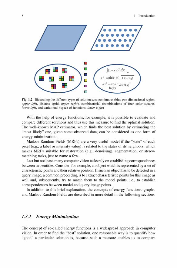
A graphical summarization of the four different types of solution sets can be seen

in Fig. 1.2.

1.3 Common Optimization Concepts in Computer Vision

Before taking a closer look at the diverse optimization methods, let’s first introduce

some concepts which are of relevance to optimization and, additionally, in

widespread use in computer vision.

1.3 Common Optimization Concepts in Computer Vision 7

With the help of energy functions, for example, it is possible to evaluate and

compare different solutions and thus use this measure to find the optimal solution.

The well-known MAP estimator, which finds the best solution by estimating the

“most likely” one, given some observed data, can be considered as one form of

energy minimization.

Markov Random Fields (MRFs) are a very useful model if the “state” of each

pixel (e.g., a label or intensity value) is related to the states of its neighbors, which

makes MRFs suitable for restoration (e.g., denoising), segmentation, or stereo-

matching tasks, just to name a few.

Last but not least, many computer vision tasks rely on establishing correspondences

between two entities. Consider, for example, an object which is represented by a set of

characteristic points and their relative position. If such an object has to be detected in a

query image, a common proceeding is to extract characteristic points for this image as

well and, subsequently, try to match them to the model points, i.e., to establish

correspondences between model and query image points.

In addition to this brief explanation, the concepts of energy functions, graphs,

and Markov Random Fields are described in more detail in the following sections.

1.3.1 Energy Minimization

The concept of so-called energy functions is a widespread approach in computer

vision. In order to find the “best” solution, one reasonable way is to quantify how

“good” a particular solution is, because such a measure enables us to compare

(x − x 0 )2 dx

(x − x 0 )

ax2 + bx + c

e x tanh(c x )

c

ln(x)sin(x)

Fig. 1.2 Illustrating the different types of solution sets: continuous (blue two-dimensional region,

upper left), discrete (grid, upper right), combinatorial (combinations of four color squares,

lower left), and variational (space of functions, lower right)

8 1 Introduction

different solutions and select the “best”. Energy functions E are widely used in this

context (see, e.g., [6]).

Generally speaking, the “energy” is a measure how plausible a solution is. High

energies indicate bad solutions, whereas a low energy signalizes that a particular

solution is suitable for explaining some observed data. Some energies are so-called

functionals. The term “functional” is used for operators which map a functional

relationship to a scalar value (which is the energy here), i.e., take a function as

argument (which can, e.g., be discretely represented by a vector of values) and

derive a scalar value from this. Functionals are needed in variational optimization,

for example.

With the help of such a function, a specific energy can be assigned to each

element of the solution space. In this context, optimization amounts to finding the

argument which minimizes the function:

x� ¼ argminx2S

EðxÞ (1.2)

As already mentioned in the previous section, E typically consists of two

components:

1. A data-driven or external energy Eext , which measures how “good” a solution

explains the observed data. In restoration tasks, for example, Eext depends on the

fidelity of the reconstructed signal R to the observed data I.2. An internal energyEint, which exclusively depends on the proposed solution (i.e.,

is independent on the observed data) and quantifies its plausibility. This is the

point where a priori knowledge is considered: based on general considerations,

we can consider some solutions to be more likely than others and therefore

assign a low internal energy to them. In this context it is often assumed that the

solution should be “smooth” in a certain sense. In restoration, for example, the

proposed solution should contain large areas with uniform or very smoothly

varying intensity, and therefore Eint depends on some norm of the sum of the

gradients between adjacent pixels.

Overall, we can write:

E ¼ Eext þ λ � Eint (1.3)

where the parameter λ specifies the relative weighting between external and

internal energy. High values of λ tend to produce smoothly varying optimization

results (if Eint measures the smoothness of the solution), whereas low values of λfavor results being close to the observed values.

Please observe that the so-called MAP (maximum a posteriori) estimation,

which is widely used, too, is closely related to energy minimization. MAP estima-

tion tries to maximize the probability p M Djð Þ of some model M , given some

observed data D (p M Djð Þ is called the posterior probability, because it denotes a


probability after observing the data). However, it is difficult to quantify p M Djð Þ inpractice. A way out is to apply Bayes’ rule:

p M Djð Þ ¼ p D Mjð Þ � pðMÞpðDÞ (1.4)

where p D Mjð Þ is called the likelihood of the data and pðMÞ the prior, whichmeasures how probable a certain model is.

If we are only interested in finding the most likely model M� (and not in the

absolute value of the posterior at this position M� ), we can drop pðDÞ and,

additionally, take the logarithm of both sides of (1.4). As a common way to

model the probabilities are Gaussian distributions, taking the logarithm simplifies

calculations considerably, because it eliminates the exponentials. If we take the

negative logarithm, we have:

M� ¼ argmin � log p D Mjð Þ½ � � log pðMÞ½ �ð Þ (1.5)

If we set Eext ¼ � log p D Mjð Þ½ � and Eint ¼ � log pðMÞ½ � , we can see that the

structure of (1.5) is the same as we encountered in (1.2).

However, please note that MAP estimation is not completely equivalent to

energy-based optimization in every case, as there are many possibilities how to

model the terms of the energy functional, and the derivation from MAP estimation

is just one kind, albeit a very principled one. Because of this principled proceeding,

Bayesian modeling has several potential advantages over user-defined energy

functionals, such as:

• The parameters of probability distributions can be learned from a set of

examples, which in general is more accurate than just estimating or manually

setting weights of the energy functional, at least if a suitable training base is

available.

• It is possible to estimate complete probability distributions over the unknowns

instead of determining one single value for each of them at the optimum.

• There exist techniques for optimizing unordered variables (e.g., the labels

assigned to different regions in image segmentation tasks) with MAP

estimations, whereas unordered variables pose a serious problem when they

have to be compared in an energy function.

1.3.2 Graphs

The concept of graphs can be found in various vision applications. In the context of

optimization, graphs can be used to model the problem at hand. An optimization

procedure being based on a graph model can then utilize specific characteristics of

the graph – such as a special structure – in order to get a fast result. In the following,

10 1 Introduction

some definitions concerning graphs and their properties are introduced (a more

detailed introduction can be found in, e.g., [4]).

A graph G ¼ N;Ef g is a set of nodes N ¼ n1; n2; . . . ; nLf g , which are also

called vertices. The nodes are connected by edges, where the edges model the

relationship between the nodes: Two nodes ni and nj are connected by an edge eijif they have a special relationship. All edges are pooled in the edge set E ¼ eij

� �

(see the left of Fig. 1.3 with circles as nodes and lines as edges for an example).

Graphs are suitable for modeling a wide variety of computer vision problems.

Typically, the nodes model individual pixels or features derived from the image,

such as interest points. The edges model the relationship between the pixels and

features. For example, an edge eij indicates that the pixels i and j influence each

other. In many cases this influence is limited to a rather small local neighborhood or

adjacent pixels. Consequently, edges are confined to nearby or, even more restric-

tive, adjoining pixels.

Additionally, an edge can feature a direction, i.e., the edge eij can point from

node ni to node nj, e.g., because pixel i influences pixel j, but not vice versa. In that

case, we talk about a directed graph (otherwise the graph is called undirected).Moreover, a weight wij can be associated to an edge eij. The weights serve as a

measure how strongly two nodes are connected.

A path in a graph from node ni to node nk denotes a sequence of nodes starting atni and ending at nk, where two consecutive nodes are connected by an edge at a time

(see blue nodes/red edges in the middle part of Fig. 1.3). If ni is equal to nk, i.e., startnode and termination node are the same, the path is termed a cycle (right part ofFig. 1.3). The length of the path is the sum of the weights of all edges along the path.

An important special case of graphs are trees. A graph is said to be a tree if it isundirected, contains no cycles, and, additionally, is connected, which means that

there is a path between any two nodes of the graph (see left of Fig. 1.4). In a tree,

one node can be arbitrarily picked as root node (light red node in right tree of

Fig. 1.4). All other nodes have a certain depth from the root, which is related to the

number of edges along the path between them and the root (as depth increases, color

saturation of the circles decreases in the right part of Fig. 1.4).Another subclass of graphs are bipartite graphs. A graph is said to be bipartite if

its nodes can be split into two disjoint subsets A and B such that any edge of the

Fig. 1.3 Exemplifying a graph consisting of nodes (circles), which are linked by edges (lines)(left). In the graph shown in themiddle, the blue nodes form a path, which are connected by the rededges. Right: example of a cycle (blue nodes, green edges)


graph connects one node of A to one node of B . This means that for any edge,

exactly one of the nodes it connects is an element ofA and exactly one is an element

of B (see left part of Fig. 1.5, where the nodes are split by the edges into the blueand the green subset). Bipartite graphs can be useful for so-called assignment

problems, where a set of features has to be matched to another feature set, i.e.,

for each feature of one set, the “best corresponding” feature of the other set has to

be found.

Last but not least, we talk about a matching M, ifM is a subset of the edge set Ewith the property that each node of the bipartite graph belongs to at most one

edge of M (see right part of Fig. 1.5). If each node is connected by exactly one

edge 2 M, M is said to be a perfect matching. Observe that the red edge set of

the right graph of Fig. 1.5 is not a perfect matching, because some nodes are not

connected to any of the red edges.

1.3.3 Markov Random Fields

One example of graphs are so-called Markov Random Fields (orMRFs), which are

two-dimensional lattices of variables and were introduced for vision applications by

[3]. Over the years, they found widespread use in computer vision (see, e.g., [1] for

an overview).

In computer vision tasks, it is natural to regard each of those variables as

one pixel of an image. Each variable can be interpreted as one node ni of a graphG ¼ N;Ef g consisting of a set of nodesN, which are connected by a set of edges E,as described in the previous section. The value each pixel takes is referred to the

state of the corresponding node.

Fig. 1.4 Showing a tree example (left). Right: same tree, with specification of a root node

(light red). Depending on their depth, the nodes get increasingly darker

Fig. 1.5 Illustrating a bipartite graph (left), where the edges split the nodes into the two blue andgreen subsets (separated by dashed red line). Right: the same bipartite graph, with a matching

example (red edges)

12 1 Introduction

In practice, the state of each node (pixel) is influenced by other nodes (pixels).

This influence is represented in the MRF through edges: if two nodes ni and njinfluence each other, they are connected by an edge eij . Without giving the exact

mathematical definition here, we note that the nature of MRFs defines that:

• Each node ni is influenced only by a well-defined neighborhood S nið Þ around it,

e.g., 4-neighborhood.

• If nj 2 S nið Þ , the relation ni 2 S nj� �

is also true, i.e., if nj is within the local

neighborhood of ni , then the same observation holds vice versa: ni is locatedwithin the neighborhood of nj.

A weight sij can be assigned to each edge eij . The sij determines how strong

neighboring nodes influence each other and are called pairwise interactionpotentials. Another characteristic of Markovian models is that a future state of a

node depends only on the current states of the nodes in the neighborhood. In other

words, there is no direct dependency (on past states of them).

Normally, the nodes N represent “hidden” variables, which cannot be measured

directly. However, each ni can be related to a variable oi which is observable. Each

ni; oið Þ pair is connected by an edge, too. A weight wi can be assigned to each of

these edges as well, and eachwi defines how strong the state of ni is influenced by oi.Markov Random Fields are well suited for Bayesian-modeled energy functionals

as introduced in the previous section and in particular for reconstruction or restora-

tion problems: Given a measured image I, which is corrupted by noise, blur, etc.,

consider the task to reconstruct its uncorrupted version R. In order to represent this

problem with an MRF, we make the following assignments:

• Each node (hidden variable) represents one unknown of the optimization prob-

lem, i.e., the state of a particular node ni represents the (unknown) value R xi; yið Þof the pixel xi; yi½ � of the image to be reconstructed.

• EachR xi; yið Þ is related to the measured value at this position I xi; yið Þ, i.e., each oiis assigned to one observed value I xi; yið Þ.

• The weightw xi; yið Þmodels how strong R xi; yið Þ is influenced by the observationI xi; yið Þ . Therefore, high values of w ensure a high fidelity of the R to the

measured image data. This corresponds to the relative weighting of the external

energy (see parameter λ in (1.3)).

• The edges eij between the hidden variables can be considered as a way of

modeling the influence of the prior probability. One way to do this is to compare

the values of neighboring hidden variables (cf. the smoothness assumption,

where low intensity differences between adjacent pixels are considered more

likely than high differences). In doing so, the weights sij determine which

neighbors influence a particular hidden variable and how strong they do this.

Due to its simplicity, it is tempting to use a 4-neighborhood. In many cases, this

simple neighborhood proves to be sufficient enough for modeling reality, which

makes it the method of choice for many applications.

If we assume a 4-neighborhood, we can model the MRF graphically as

demonstrated in Fig. 1.6. The grid of hidden variables, where each variable represents


a pixel, is shown on the left side of the figure. The right side of the figure illustrates a

(zoomed) part of the MRF (red) in more detail. The hidden variables are illustrated

via white circles. Each hidden variable is connected to its four neighbors via edges

with weights sx and sy (symbolized by white squares). An observed data value (gray

circles) is associated to each hidden variable with weight w (gray square). It is

possible to utilize spatially varying weightssx x; yð Þ,sy x; yð Þ, andw x; yð Þ, if desired, butin many cases it is sufficient to use weights being constant over the entire MRF.

If the MRF models an energy functional, the following relationships are

frequently used: The external or data-driven energy Eext x; yð Þ of each pixel

depends on the difference between the state of the hidden variable and the

observed value:

Eext x; yð Þ ¼ w x; yð Þ � ρext R x; yð Þ � I x; yð Þð Þ (1.6)

The energy being based on the prior follows a smoothness assumption and

therefore penalizes adjacent hidden variables of highly differing states:

Eint x; yð Þ ¼sx x; yð Þ � ρint I x; yð Þ � I xþ 1; yð Þð Þ þ sy x; yð Þ�ρint I x; yð Þ � I x; yþ 1ð Þð Þ (1.7)

In both (1.6) and (1.7), ρ denotes a monotonically increasing function, e.g., a

linear (total variation) penalty ρðdÞ ¼ dj j or a quadratic penalty ρðdÞ ¼ dj j2. In the

case of quadratic penalties, we talk about Gaussian Markov Random Fields

(GMRFs), because quadratic penalties are best suited when the corruption of the

observed signal is assumed to be of Gaussian nature.

However, in many cases, a significant fraction of measurements is disturbed by

outliers with gross errors, and a quadratic weighting puts too much emphasis on the

influence of these outliers. Therefore, hyper-Laplacian penalties of the type ρðdÞ ¼dj jp; p < 1 are also common.

Fig. 1.6 Showing a graphical illustration of a Markov Random Field (left) and a more detailed

illustration of a part of it (right)

14 1 Introduction

The total energy associated to the current state of an MRF equals the sum of the

external as well as internal energy terms over all pixels:

EMRF ¼X

x;y

Eint x; yð Þ þX

x;y

Eext x; yð Þ (1.8)

Minimization of these types of MRF-based energies used to be performed by a

method called simulated annealing (cf. [5]) when MRFs were introduced to the

vision community (see [3]). Simulated annealing is an iterative scheme which, at

each iteration, randomly picks a variable which is to be changed in this iteration. In

later stages, the algorithm is rather “greedy,” which means that it has a strong bias

toward changes which reduce the energy. In early stages, however, a larger fraction

of changes which does not immediately lead to lower energies is allowed. The

justification for this is that the possibility to allow changes which increase the

energy helps to avoid being “trapped” in a local minimum of the energy functional.

In the meantime, however, it was shown that another class of algorithm called

graph cuts is better suited for optimization and outperforms simulated annealing in

most vision applications (see, e.g., [2]). Here, the algorithm works on the graph

representation of the MRF and intends to find a “cut” which separates the graph into

two parts where the total sum of the weights of edges to be cut attains a minimum.

MRFs have become popular to model problems where a reasonable prior is to

assume that the function to be found varies smoothly. Therefore, it can be

hypothesized that each pixel has a high probability to take values identical or

very similar to its neighbors, and this can be modeled very well with an MRF.

Apart from the already mentioned restoration task, MRFs are also suited for

segmentation, because it is unlikely that the segmentation label (all pixels belong-

ing to the same region are “labeled” with identical value) changes frequently

between neighboring pixels, which would result in a very fragmented image. The

same fact applies for stereo matching tasks, where the disparity between associated

pixels, which is a measure of depth of the scene, should vary slowly spatially.

A variant of MRFs are so-called conditional random fields (CRF), which differ

from standard MRFs in the influence of the observed data values: More specifically,

the weights of the pairwise interaction potentials can be affected by the observed

values of the neighboring pixels (see Fig. 1.7). In that case, the prior depends not

Fig. 1.7 Illustrating the

structure of a so-called

conditional random field.

The influence of the observed

data values on the pairwise

interaction weights to

neighboring nodes is

indicated by red lines


only on the hidden variables but additionally on the sensed data in the vicinity of

each pixel.

The answer to the question whether an MRF or CRF is better depends on the

application. For some applications, the additional connections between observed

data values and the prior (which for MRFs do not exist) are advantageous. For

example, we can observe that the smoothness assumption of MRFs has a bias

toward slowly varying states of the hidden variables, which is not desirable in the

presence of edges, because then they are smoothed, too. If, however, the smooth-

ness weights sx x; yð Þ and sy x; yð Þ are reduced for pixels where a strong edge is

present in the observed data, these edges are more likely to be preserved. Hence,

CRFs are one means of attenuating this bias.

References

1. Blake A, Kohli P, Rother C (2011) Markov random fields for vision and image processing. MIT

Press, Cambridge, MA. ISBN 978-0262015776

2. Boykov J, Veksler O, Zabih R (2001) Fast approximate energy minimization via graph cuts.

IEEE Trans Pattern Anal Mach Intell 23(11):1222–1239

3. Geman S, Geman D (1984) Stochastic relaxation, Gibbs distributions, and the Bayesian

restoration if images. IEEE Trans Pattern Anal Mach Intell 6(6):721–741

4. Gross JL, Yellen J (2005) Graph theory and its applications, 2nd edn. Chapman & Hall/CRC,

Boca Raton. ISBN 978-1584885054

5. Kirkpatrick S, Gelatt CD, Vecchi MP (1983) Optimization by simulated annealing. Science 220

(4598):671–680

6. Rangarajan A, Vemuri B, Yuille A (eds) (2005) Energy minimization methods in computer

vision and pattern recognition: 5th international workshop (proceedings). Springer, Berlin.

ISBN 978-3540302872

7. Velho L, Gomes J, Pinto Carvalho PC (2008) Mathematical optimization in computer graphics

and vision. Morgan Kaufmann, Amsterdam. ISBN 978-0127159515

16 1 Introduction

Chapter 2

Continuous Optimization

Abstract A very general approach to optimization are local search methods, where

one or, more typically, multiple variables to be optimized are allowed to take

continuous values. There exist numerous approaches aiming at finding the set of

values which optimize (i.e., minimize or maximize) a certain objective function. The

most straightforward way is possible if the objective function is a quadratic form,

because then taking its first derivative and setting it to zero leads to a linear system of

equations, which can be solved in one step. This proceeding is employed in linear

least squares regression, e.g., where observed data is to be approximated by a

function being linear in the design variables. More general functions can be tackled

by iterative schemes, where the two steps of first specifying a promising search

direction and subsequently performing a one-dimensional optimization along this

direction are repeated iteratively until convergence. These methods can be

categorized according to the extent of information about the derivatives of the

objective function they utilize into zero-order, first-order, and second-order methods.

Schemes for both steps of the general proceeding are treated in this chapter.

In continuous optimization problems, the solution set S is a continuous subset of Rn.

Usually we have n > 1, and, therefore, we talk about multidimensional optimiza-

tion. The nature of this kind of optimization problem is well understood, and there

exist numerous methods for solving this task (see, e.g., [3] for a comprehensive

overview). In order to find the most appropriate technique for a given problem, it is

advisable (as always in optimization) to consider as much knowledge about the

specific nature of the problem at hand as possible, because this specific knowledge

usually leads to (sometimes dramatically) faster as well as more accurate solutions.

Hence, the techniques presented in the following are structured according to

their specific characteristics. Starting with the special case of regression, where the

problem leads to a quadratic form, we move on to more general techniques which

perform an iterative local search. They differ in the knowledge available about first-

and second-order derivatives of the objective function. Clearly, additional



17

knowledge about derivatives helps in speeding up the process in terms of iterations

needed, but may not be available or time-consuming to calculate.

2.1 Regression

2.1.1 General Concept

A special case of objective functions f xð Þ are quadratic forms, where the maximum

order in the design variables is two. In multidimensional optimization, a quadratic

objective function can be written as

f xð Þ ¼ 12� xT �H � x� aT � xþ c (2.1)

The minimum of such an objective function can be found analytically by setting

its first derivative @f xð Þ @x= to zero. This leads to a system of linear equations

H � x� ¼ a (2.2)

with x� being the desired minimizer of f xð Þ. x� can be obtained by solving the linearequation system (2.2) using standard techniques. Please observe that @f xð Þ @x= ¼ 0

is just a necessary condition that f xð Þ takes a minimal value at x� (e.g., a point withzero derivative could also be a maximum or a saddle point). However, by design of

f xð Þ it is usually assured that f xð Þ has a unique minimum.

Obtaining a proper (unique) solution of (2.2) is possible if the so-called pseudo-

inverseHþ exists. This is fulfilled if the columns ofH are linearly independent. We

will come back to this point later when we see how H is built during regression.

Now let’s turn to regression. The goal of regression is to approximate observed

data by some function. The kind/structure of the function is usually specified in

advance (e.g., a polynomial of order up to seven), and hence, the remaining task is

to determine the coefficients of the function such that it fits best to the data.

As we will see shortly, regression problems can be turned into quadratic optimi-

zation problems if the function is linear in the coefficients to be found. A typical

example is an approximation of observed data gðxÞ by a polynomial pðxÞ ¼ c0 þ c1�xþ c2 � x2 þ � � � þ cn � xn, which is performed quite often in practice. Clearly, this

function is linear in its coefficients. A generalization to the multidimensional case

where x is a vector is straightforward.

Now the task of polynomial regression is to determine the coefficients such that

the discrepancy between the function and the observed data becomes minimal.

A common measure of the error is the sum of the squared differences (SSD)

between the observed data g xið Þ and the values p c; xið Þ of the approximation

function (which is a polynomial in our case) at these positions xi . Consequently,this sum of squared differences is to be minimized. Therefore, we talk about least

18 2 Continuous Optimization

squares regression. Under certain reasonable assumptions about the error being

introduced when observing the data (e.g., noise), the least squares solution

minimizes the variance of the errors while keeping the mean error at zero at the

same time (unbiased error). Altogether, the objective function in polynomial least

squares regression can be formulated as

fR cð Þ ¼XN

i¼1p c; xið Þ � g xið Þj j2 (2.3)

where g xið Þ is a measured data value at position xi andN denotes the number of data

values available. As can easily be seen, fR cð Þ is a quadratic form in c (as it is a

summation of terms containing powers of the ci’s up to order two), and, therefore,

its minimizer c� can be determined by the solution of a suitable system of linear

equations.

2.1.2 Example: Shading Correction

In order to show how this works in detail, let’s consider an image processing

example named shading correction: Due to inhomogeneous illumination as well

as optical effects, the observed intensity values often decrease at image borders,

even if the camera image depicts a target of uniform reflectivity which should

appear uniformly bright all over the image. This undesirable effect can be

compensated by determining the intensity decline at the image borders (shading)

with the help of a uniformly bright target. To this end, the decline is approximated

by a polynomial function pS c; xð Þ. Based on this polynomial, a correction function

lS xð Þ can be derived such that pS c; xð Þ � lS xð Þ � 1 for every pixel position x .Subsequently, lS xð Þ can be used in order to compensate the influence of shading.

The first question to be answered is what kind of polynomial pS c; xð Þwe choose.This function should be simple, but approximate the expected shading well at the

same time. Typically, shading is symmetrical to the center of the camera image.

Therefore, it suffices to include terms of even order only in pS c; xð Þ if x specifies theposition with respect to the camera center. Next, in order to limit the number of

coefficients c; it is assumed that a maximum order of four is sufficient for pS c; xð Þbeing a good approximation to observed shading. Hence, we can define pS c; xð Þ asfollows:

pS c; xð Þ ¼c0 þ c1 � u2 þ c2 � v2 þ c3 � u2 � v2 þ c4 � u4þþ c5 � v4 þ c6 � u4 � v2 þ c7 � u2 � v4 þ c8 � u4 � v4

(2.4)

where u ¼ x� xcj j y and v ¼ y� ycj j denote the pixel distances to the image center

xc; yc½ � in x- and y -directions. Altogether, we have nine parameters c0 to c8, whosenumerical values are to be determined during regression. Consequently, c0 to c8 actas design variables in the optimization step.

2.1 Regression 19

In order to generate data values to which we can fit pS c; xð Þ, we take an image of

a special target with well-defined and uniform brightness and surface properties

(which should appear with uniform intensity in the camera image if shading was not

present). As we want to be independent of the absolute intensity level, we take the

observed intensity values I xð Þ normalized with respect to the maximum observed

intensity:

~I xð Þ ¼ I xð ÞImax

Our goal is to find a parameter setting c such that pS c; xð Þ approximates the

normalized intensities well. Hence, we can write ~I xð Þ ¼ pS c; xð Þ þ eor, equivalently,

1 u2 v2 . . . u4v4� � �

c0c1...

c8

26664

37775 ¼

~I xð Þ þ e (2.5)

where e denotes the error to be minimized. If we compare observed data values and

the polynomial at different locations xi; i 2 1 . . .N½ � , we can build one equation

according to (2.5) for each data point i and stack them into a system ofN equations:

1 u12 v1

2 u12v1

2 u14 v1

4 u14v1

2 u12v1

4 u14v1

4

1 u22 v2

2 u24v2

4 u24 v2

4 u24v2

2 u22v2

4 u24v2

4

..

. ... ..

. ... ..

. ... ..

. ... ..

.

1 uN2 vN

2 uN2vN

2 uN4 vN

4 uN4vN

2 uN2vN

4 uN4vN

4

266664

377775�

c0

c1

..

.

c8

266664

377775�

~I x1ð Þ~I x2ð Þ...

~I xNð Þ

266664

377775

or X � c � d

(2.6)

where the matrix X summarizes the position information and the data vector d is

composed of the normalized observed intensity values ~I.The goal of regression in this case is to find some coefficients c� such that the

sum of squared distances between the observed ~I and their approximation X � c� isminimized:

c� ¼ argmin X � c� dk k2 (2.7)

This minimizer c� of this quadratic form can be found by setting the derivative

@ X � c� dk k2 @c= to zero, which leads to

XT � X � c� ¼ XT � d (2.8)


which is called the normal equation of the least squares problem. A solution is

possible ifXT � X is non-singular, i.e.,XT � Xhas linearly independent columns. This

constraint can be fulfilled by a proper choice of the positions u; v½ �. In that case, thepseudo-inverse exists and the solution is unique.

The system of normal equations can be solved by performing either a LR or QR

decomposition of XT � X (e.g., see [6]). The former has the advantage of being

faster, whereas the latter is usually numerically more stable, especially if the matrix

XT � X is almost singular. Another way to find c� is to calculate the pseudo-inverse

XT � X� �þby performing a singular value decomposition (SVD) of XT � X [6].

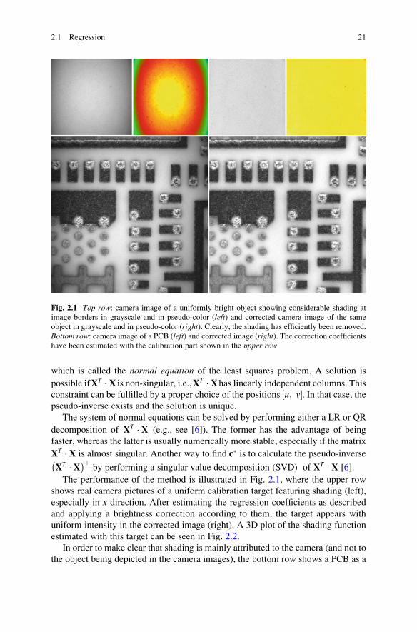
The performance of the method is illustrated in Fig. 2.1, where the upper row

shows real camera pictures of a uniform calibration target featuring shading (left),

especially in x-direction. After estimating the regression coefficients as described

and applying a brightness correction according to them, the target appears with

uniform intensity in the corrected image (right). A 3D plot of the shading function

estimated with this target can be seen in Fig. 2.2.

In order to make clear that shading is mainly attributed to the camera (and not to

the object being depicted in the camera images), the bottom row shows a PCB as a

Fig. 2.1 Top row: camera image of a uniformly bright object showing considerable shading at

image borders in grayscale and in pseudo-color (left) and corrected camera image of the same

object in grayscale and in pseudo-color (right). Clearly, the shading has efficiently been removed.

Bottom row: camera image of a PCB (left) and corrected image (right). The correction coefficientshave been estimated with the calibration part shown in the upper row

2.1 Regression 21

highly structured object, where shading is clearly visible. The right image shows the

same PCB after correction according to the coefficients calculated through the

usage of the calibration target. Observe that the background of the PCB appears

uniformly bright after correction, so the results obtained with the calibration target

can be transferred to other objects as well.

The matrix X is of dimensionality M � N , which means that we have M

unknowns (the coefficients of the polynomial) and N equations. Hence, XT � X is of

dimensionality N � N. In order to get a unique solution, it has to be ensured that we

have at least as much equations than unknowns, i.e., N M. Usually however, there

are so many data points available such that N >> M , which would mean that

the system of normal equations to be solved would become extremely large. Consider

the shading example: if we took every pixel as a separate data value,Nwould be in the

order of hundreds of thousands or millions. In order to get to manageable data sizes,

the image can be partitioned into horizontal as well as vertical tiles. For each tile,

a mean intensity value can be calculated, which serves as input for (2.6). The tile

position is assumed to be the center position of the tile. Taking just the mean value of

the tiles significantly reduces N and also reduces the noise influence drastically.

2.2 Iterative Multidimensional Optimization:General Proceeding

The techniques presented in this chapter are universally applicable, because they:

• Directly operate on the energy function f ðxÞ.• Do not rely on a special structure of f ðxÞ.

The broadest possible applicability can be achieved if only information about the

values of f ðxÞ themselves is required.

Fig. 2.2 Plot of the

estimated shading function

based on regression of the

intensity data of the upperleft image of Fig. 2.1


The other side of the coin is that these methods are usually rather slow.

Therefore, some of the methods of the following sections additionally utilize

knowledge about the first- and second-order derivatives f 0ðxÞ and f 00ðxÞ . Thisrestricts their applicability a bit in exchange for an acceleration of the solution

calculation. As was already stated earlier, it usually is best to make use of as much

specific knowledge about the optimization problem at hand as possible. The usage

of this knowledge will typically lead to faster algorithms.

Furthermore, as the methods of this chapter typically perform a local search,there is no guarantee that the global optimum is found. In order to avoid to get stuck

in a local minimum, a reasonably good first estimate x0 of the minimal position x� isrequired for those methods.

The general proceeding of most of the methods presented in this chapter is

a two-stage iterative approach. Usually, the function f xð Þ is vector valued, i.e., xconsists of multiple (sayN) elements. Hence, the optimization procedure has to findN

values simultaneously. Starting at an initial solutionxk, this can be done by an iteratedapplication of the following two steps:

1. Calculation of a so-called search direction sk along which the minimal position is

to be searched.

2. Update the solution by finding a xkþ1 which reduces f xkþ1� �

(compared to f xk� �

)

by performing a one-dimensional search along the direction sk . Because sk

remains fixed during one iteration, this step is also called a line search.

Mathematically, this can be written as

xkþ1 ¼ xk þ αk � sk (2.9)

where, in the most simple case, αk is a fixed step size or – more sophisticated – is

estimated during the one-dimensional search such that xkþ1 minimizes the objective

function along the search direction sk . The repeated procedure stops either if

convergence is achieved, i.e., f xkþ1� �

is sufficiently close to f xk� �

and hence we

assume that no more progress is possible, or if the number of iterations exceeds an

upper thresholdKmax. This iterative process is visualized in Fig. 2.3 with the help of

a rather simple example objective function.

As should have become apparent, this proceeding basically involves performing

a local search, meaning that there is no guarantee that the global minimum of f xð Þ isfound. However, in most cases of course, the global optimum would be the desired

solution. In order to be sure that a local minimum also is the global one, the function

has to be convex, i.e., the following inequality has to hold for everyx1; x2 2 R N and

0 < λ < 1:

f λ � x1 þ 1� λð Þ � x2ð Þ λ � f x1ð Þ þ 1� λð Þ � f x2ð Þ (2.10)

For most problems, convexity is only ensured in a limited area of the solution

space, which is called the area of convergence. As a consequence, the iterative local

2.2 Iterative Multidimensional Optimization: General Proceeding 23

search methods presented below rely on a sufficiently “good” initial solution x0 ,which is located within the area of convergence of the global optimum. This also

means that despite being applicable to arbitrary objective functions f xð Þ , localsearch methods are typically not suited to optimize highly non-convex functions,

because then the area of convergence is very small and, as a result, there is a large

risk that the local search gets stuck in a local minimum being arbitrarily far away

from the desired global optimum.

In order to overcome this restriction, the local iterative search can be performed

at multiple starting points x0l ; l 2 1; 2; . . . ; L½ �. However, there still is no guarantee

that the global minimum is found. But the probability that the found solution is

sufficiently close to the true optimum is increased significantly. Of course the cost

of such a proceeding is that the total runtime of the algorithm is increased

significantly.

Methods for both parts of the iterative local search (estimation of sk and the

one-dimensional search along sk) shall be presented in more detail below. Observe

that some methods (like Newton’s method) slightly deviate from the general

proceeding just outlined, because they don’t perform a one-dimensional optimiza-

tion along the search direction, but take a step of fixed, predefined, or estimated size

in that direction instead.

Pseudocode

function optimizeContinuousMultidim (in Image I , in

objective function f xð Þ , in initial solution x0, in conver-gence criterion ε, out refined solution x�)

Fig. 2.3 Visualizing the iterative proceeding in multidimensional optimization when performing

a local search: starting from some position (black dot in left image), the search direction is

calculated first (red arrow in middle image), and then a one-dimensional optimization is performed

in this direction (result: red dot in right image). The new position serves as a starting point for the

next iteration until convergence is achieved


k 0

// main optimization looprepeat

calculate search direction sk (see section 2.2.2)

find one-dimensional minimum along direction sk (see (2.9)and section 2.2.1) OR take one step of a fixed predefined

or estimated size in the search direction, yielding xkþ1

k k þ 1

untilf xkð Þ�f xkþ1ð Þf xkð Þþf xkþ1ð Þ ε OR k > Kmax

x� xk

2.2.1 One-Dimensional Optimization Alonga Search Direction

In this section, step two of the general iterative procedure is discussed in more

detail. The outline of the proceeding of this step is to first bound the solution and

subsequently iteratively narrow down the bounds until it is possible to interpolate

the solution with good accuracy. In more detail, the one-dimensional optimization

comprises the following steps (see also flowchart of Fig. 2.4):

1. Determine upper and lower bounds xku ¼ xk þ α0u � sk and xkl ¼ xk þ α0l � sk whichbound the current solution xk (α0u and α0l have opposite signs).

2. Recalculate the upper and lower bounds xiu and xil in an iterative scheme, i.e.,

decrease the distance betweenxiu andxil as the iteration proceeds. Please note that,

for a better understanding, the superscript k indicating the index of the multidi-

mensional iteration is dropped and replaced by the index i of the current

one-dimensional iteration. One possibility to update the bounds is the so-called

golden section method, which will be presented below. As the distance between

the bounds is reduced by a fixed fraction at each iteration there, we can set the

number of iterations necessary to a fixed value N.

no

Calculate ini-tial bounds;

n=0

Update onebound (e.g.

Golden Section)

Incre-ment n

n==N?Cubic inter-pol.: Refine1D optimum

S

Eyes

Fig. 2.4 Flowchart of the golden section method


3. Refine the solution by applying a polynomial interpolation to the data found in

step 2, where the refined boundsxiu and xil as well as two intermediate points were

found (see below). Hence, we have four data points and can perform a cubic

interpolation based on these four points.

At the end of step 3, we have determined an estimate ofαk such that the update ofthe multidimensional solution can be calculated according to (2.9). Hence, the task

of one-dimensional optimization here is to find an appropriate αk. For the moment,

let’s start with a closer look at step 2 and assume that some upper as well as lower

bounds α0u and α0l are already determined by step 1.

An important point to mention is that it is assumed that the function to be

minimized is unimodal between xku and xkl . This means that it is convex and has

only one minimum in between those two points. As we already know that the

desired optimal position has to be located within the bounds x0u and x0l , the task

of step two can be interpreted as an iterative refinement of the upper and lower

bounds until the distance between those two points is sufficiently small. To this

end, the function is evaluated at two intermediate points x01 ¼ xk þ α01 � sk and x02 ¼xk þ α02 � sk. α01 and α02 are chosen such that α0l < α01 < α02 < α0u; and, therefore, itis guaranteed thatx01 andx

02 are both located within the current bounds. Furthermore,

x01 is closer to x0l than x02 is x01 � x0l�� < x02 � x0l

�� . In other words, it is ensured that

the four points x0l , x01, x

02, and x0u are strictly ordered.

Now consider the values f x01� �

and f x02� �

of the objective at the two intermediate

positions: because of the unimodality constraint, we can conclude that either f x01� �

will form a new lower bound or f x02� �

will form a new upper bound of the solution.

If f x01� �

< f x02� �

, then x02 will become a new upper bound of the solution, i.e.,

x1u ¼ x02. If f x01� �

> f x02� �

, however, then x01 will form a new lower bound of the

solution, i.e., x1l ¼ x01 (see Fig. 2.5 for both of the two cases). Hence, at each

iteration step either the lower or the upper bound is replaced by one of the two

intermediate points. A repeated application of this proceeding leads to narrower

bounds at each step. Eventually, they are so close that convergence is achieved.

Fig. 2.5 Illustrating the refinement of the bounds of the solution. The blue points indicate currentlower and upper bounds, whereas the red color of a point indicates that the point becomes a new

bound. Left: as x1 (red) takes a higher function value than x2 (green), x1 is a new lower bound.

Right: as x2 (red) takes a higher function value than x1 (green), x2 is a new upper bound


Please note that if the unimodality constraint is violated, this proceeding might get

stuck in a local minimum.

What remains to be answered is the question of where to place the intermediate

points. (From now on, we replace the superscript 0 of the above equations by the

index i, as we consider the iterated scheme now and the basic principle remains

the same for all iteration steps.) Obviously, xi1 and xi2 have to be positioned such that

the average performance of the method is optimized. To this end, the following two

criteria must hold:

• The positions xi1 and xi2 should be placed symmetric about the center of the

interval between the upper and lower bound, i.e., αiu � αi2 ¼ αi1 � αil. This is inaccordance with intuition that convergence is on average achieved fastest if the

distance between the two bounds is reduced by a fixed fraction, regardless of

whether the upper or the lower bound is altered.

• Additionally, it is desirable to minimize the number of function evaluations as

much as possible. Therefore, it is advisable to reuse the data calculated in previous

iteration steps. More specifically, if, e.g., xi1 becomes the new lower bound, then it

would be good if we could setxiþ11 ¼ xi2 (or, equivalently,αiþ11 ¼ αi2). In turn, ifx

i2

becomes the new upper bound, we must aim to set xiþ12 ¼ xi1 (or, equivalently,

αiþ12 ¼ αi1 ). In order to achieve this as well, the following relation must hold:αi1�αi

l

αiu�αil¼ αi

2�αi

1

αiu�αi1.

This leads to the following rules:

αi1 ¼ 1� τð Þ � αil þ τ � αiuαi2 ¼ 1� τð Þ � αiu þ τ � αil

with τ ¼ 3� ffiffiffi5p

2� 0:38197 (2.11)

The ratio defined by τ is called the golden section number, and therefore, this

one-dimensional search method is called golden section algorithm.In order to identify convergence, a suitable convergence criterion has to be

defined. A reasonable choice is to reduce the size of the interval between upper

and lower bound to a fixed small fraction of the size of the starting interval. By

definition of τ it is ensured that the interval is reduced by a fixed fraction at each

iteration step. Accordingly, convergence is achieved after a fixed number N of

iteration steps are performed. Taking the above value of τ into account, N can be

calculated as follows:

N � �2:078�ln εþ 3 (2.12)

where ε defines the fraction of the original interval size to be fallen below. For

example, if it is requested that convergence is achieved when the interval size is

below 0.1 % of the original size (i.e., ε ¼ 0:001), we have to perform N ¼ 18

iteration steps.

After the iteration has terminated, the values αil, αi1, α

i2, and α

iu are available. Thus,

we can use these for values for an interpolation with a cubic polynomial, as the four


coefficients of the cubic polynomial can be calculated straightforward from αil, αi1, α

i2,

andαiu as well as their function values (step three of the one-dimensional method). The

final result of one-dimensional optimization αk can be set according to that one of thepossibly two real roots of the cubic polynomial which is located in between αil and α

iu.

Now let’s come back to step one of our one-dimensional optimization scheme, the

search for the initial bounds of the one-dimensional solution. The first estimate of the

bounds can be done by taking a fixed step in the direction of sk and another one with

opposite sign, both starting from the current estimate of the minimum xk. As the step

size is somehow arbitrary, we can simply take x0l ¼ xk � sk and x0u ¼ xk þ sk. If both

f x0l� �

and f x0u� �

are larger than f xk� �

, we’re finished and the bounds are found. This

situation can be seen in the left part of Fig. 2.6: The function values of the left bound

estimate (blue, opposite to current search direction) as well as the right bound

estimate (light blue, in current search direction) are both larger than at the current

solution. Therefore, the two points can be taken as new lower and upper bounds,

respectively.

If not, the exact search direction can be defined by comparing f x0l� �

and f x0u� �

. If

f x0l� �

> f x0u� �

, the function has a negative slope in the direction of sk at xk (middle

picture in Fig. 2.6), which is usually the case if sk was chosen properly (because wewant to find a minimum, it should be expected that the slope in the search direction

is negative). We can also observe that the step size was taken too small and

therefore x0l and x0u don’t bracket the solution yet.

Therefore, we have to update x0u iteratively. To this end, set x0u as a new

intermediate point x1 ¼ x0u and update x0u according to

xjþ1u ¼ 1þ að Þ � xju � a � xjl with a ¼ 1þ ffiffiffi5p

2(2.13)

This choice of the step size a ensures that xjl, x1; and xju can be taken directly as

starting values x0l , x01; and x0u of the golden section method. Furthermore, it also

ensures that the steps increase in size from iteration to iteration such that a valid

bracketing of the minimum is achieved in reasonable time if the (arbitrary) starting

step size chosen was far too small.

Fig. 2.6 Showing three

different situations in the

calculation of the initial

lower and upper bounds,

starting from the current

solution (green dots). Thesearch direction is indicated

by gray arrows. See text fordetails


The iteration stops if f xjþ1u

� �> f x1ð Þ, because then the negative slope at x0l in the

direction ofx0u has turned into a positive one when going further in this direction and

eventually arriving at xjþ1u . If f xjþ1u

� � f x1ð Þ, then set xjþ1l ¼ x1 (because the slope

is still negative when moving from x1 to xjþ1u ) and apply (2.13) again. Take a look at

the middle part of Fig. 2.6: here, the function value of the right bound estimate is

lower than the value at the current solution. Therefore, we have to search further in

this direction until the function value becomes larger than at the current solution

(red point).

If f x0l� �

< f xk� �

< f x0u� �

, in fact we have to search the minimum in direction

opposite to sk, because now the slope in the direction of sk is positive. This can be

achieved by interchanging x0l and x0u and then applying the iterative bounds search

just described with the interchanged positions. Observe the right picture of Fig. 2.6:

here, we have the same situation as in the middle part, except that the current search

direction has the wrong sign (shown by dotted arrow and indicated by the fact that

the border estimate in search direction (light blue) takes a higher function value

compared to the value at the green position but in the opposite direction the function

value is lower (blue)). Therefore, the search direction is turned around (solid arrow)

and the iteration proceeds until a proper bound is found (red).

Pseudocode

function optimizeContinuousOnedim (in Image I, in objective

function f xð Þ, in current solution xk, in search direction sk, in

convergence criterion ε, out refined solution xkþ1)

// step 1: estimate initial lower and upper bounds xkl and xkucalculate x0l ¼ xk � sk and x0u ¼ xk þ sk

if f x0l� �

< f xk� �

< f x0u� �

then // right picture of Figure 2.6

sk � sk // invert search direction

interchange x0l and x0uend if

if f x0u� �

< f xk� �

then // middle picture of Figure 2.6

// iterative search until a “valid” upper bound is foundrepeat

j 0

x1 xjucalculate xjþ1u according to (2.13)j jþ 1

until f xju� �

> f xk� �

end if

// iterative refinement of the bounds (golden section method)calculate N according to (2.12)

calculate α0l and α0u, based on xjl, xju, and sk.


calculate x01 (if not known already) and x02 by determining α01 andα02 according to (2.11)for i ¼ 0 to N � 1

if f xi1� �

< f xi2� �

then

// new upper bound found

xiþ1u xi2xiþ12 xi1calculate xiþ11 by determining αiþ11 according to (2.11)

else// new lower bound found

xiþ1l xi1xiþ11 xi2calculate xiþ12 by determining αiþ12 according to (2.11)

end ifnext

// final refinement of solution by cubic interpolation

calculate xkþ1 based on cubic interpolation at the four points

xil, xi1, xi2, and xiu

2.2.2 Calculation of the Search Direction

The choice of the search direction is very important for the runtime performance of

the entire optimization method, because the total number of one-dimensional

optimization steps is to a large extent influenced by this choice. Hence, a proper

choice of the search direction plays an important role in the algorithm design.

Having this in mind, some algorithms are designed such that they try to make use

of the performance of the past steps when the search direction of the current

optimization step is estimated. Apart from that, it is advisable to incorporate as

much knowledge about the objective function f xð Þas possible. One way to do this isto make use of the derivatives of f xð Þ . In fact, optimization methods can be

categorized according to the maximum order of the derivatives they make use of:

• Zero-order methods: The search directions sk are calculated solely based on f xð Þitself; no derivative information is taken into account.

• First-order methods: The gradientrf xð Þ is also considered in the calculations ofsk.• Second-order methods: Here the matrix H xð Þ consisting of the second-order

derivatives (also called Hessian matrix) influences the search direction sk, too.

The gradient rf xð Þ is defined as

rf xð Þ ¼ @f

@x1;@f

@x2; . . . ;

@f

@xN

� T(2.14)


where N denotes the number of elements of the vector x. The Hessian matrix H xð Þcan be written as

H xð Þ ¼@2f

@x1@x1� � � @2f

@x1@xN

..

. . .. ..

.

@2f@xN@x1

� � � @2f@xN@xN

2664

3775 (2.15)

As can easily be seen, H xð Þ is symmetric.

Clearly, the more derivative information is taken into account, the fewer itera-

tion steps should be needed. Bear in mind, however, that the additional calculation/

estimation of the derivatives itself takes time, too. Apart from that, it might not be

possible to calculate the derivatives analytically in some cases, or their numerical

estimation might be error-prone. Therefore, methods of all three categories men-

tioned above have its justification and some representatives of each category will be

presented in the following sections.

2.3 Second-Order Optimization

2.3.1 Newton’s Method

Newton’s method is a classical example of second-order continuous optimization

(see, e.g., [2] for a more detailed description). Here, the function f xð Þ is

approximated by a second-order Taylor expansion T at the current solution xk:

f xð Þ ffi T δxð Þ ¼ f xk� �þrf xk

� � � δxþ 1

2δxT �H xk

� � � δx (2.16)

with δx being the difference x� xk. As long as δx remains sufficiently small, we can

be quite sure that the second-order Taylor expansion T δxð Þ is a sufficiently good

approximation of f xð Þ.As f xð Þ is approximated by a quadratic form, a candidate of its minimum can be

found analytically in a single step by setting the derivative of the quadratic form to

zero. This yields a linear system of equations which can be solved with standard

techniques (see also Sect. 2.1). Because the Taylor expansion is just an approxima-

tion of f xð Þ, its minimization at a single position is usually not sufficient for finding

the desired solution. Hence, finding a local minimum of f xð Þ involves an iterative

application of the following two steps:

1. Approximate f xð Þ by a second-order Taylor expansion T δxð Þ (see (2.16)).2. Calculate the minimizing argumentδx� of this approximationT δxð Þby setting its

first derivative to zero: rT δxð Þ ¼ 0

2.3 Second-Order Optimization 31

In order for δx� to be a local minimum of T δxð Þ, the following two conditions

must hold:

1. rT δx�ð Þ ¼ 0:

2. H xk� �

is positive, i.e., dT �H xk� � � d > 0 for every vector d. This is equivalent to

the statement that all eigenvalues of H xk� �

are positive real numbers. This

condition corresponds to the fact that for one-dimensional functions, their

second derivative has to be positive at a local minimum.

Now let’s see how the two steps of Newton’s method can be implemented in

practice. First, a differentiation of T δxð Þ with respect to δx yields:

rf xð Þ ffi rT δxð Þ ¼ rf xk� �þH xk

� � � δx (2.17)

Setting (2.17) to zero leads to the following linear system of equations:

H xk� � � δx ¼ �rf xk

� �(2.18)

The minimizer δx� of (2.18) can be found by, e.g., a QR or LR decomposition of

the matrix of the normal equation of (2.18) or directly via a singular value

decomposition of H xk� �

(see, e.g., [6]). Now that δx� is found, the solution can

be updated as follows:

xkþ1 ¼ xk þ δx� (2.19)

In the notion of (2.9), we can alternatively formulate the following update rule

for Newton’s method:

xkþ1 ¼ xk �H xk� ��1 � rf xk

� �; i:e: sk ¼ �H xk

� ��1 � rf xk� �

(2.20)

As far as implementation is concerned, (2.20), which involves explicitly calcu-

lating the inverseH xk� ��1

, is not applied. The linear equation system (2.18) is solved

instead. Note also that no separate one-dimensional optimization is performed in this

method. Instead, the direction as well as the step size are estimated together in one

step, as can be seen in (2.20). The whole process is summarized in Fig. 2.7.

Please observe that Newton’s method has only a limited area of convergence,

i.e., the initial solution x0 has to be sufficiently close to the true minimum of f x�ð Þ,because T δxð Þ is a sufficiently good approximation of f xð Þ in just a limited local

neighborhood around the optimum. This also relates to the fact that the second of

the above-mentioned conditions has to be fulfilled (positivity of the Hessian): if we

are too far away from the minimum, the Hessian might not be positive any longer.

Please note that this condition is not checked explicitly in the method, and

consequently, if the condition is violated, the method will have poor performance.

On the other hand, the convergence of Newton’s method is very fast. Therefore, it is

well suited for a fast and accurate refinement of a sufficiently “good” initial

solution.


Pseudocode

function optimizeMultidimNewton (in Image I, in objective

function f xð Þ, in initial solution x0, in convergence crite-rion ε, out final solution x�)

// main search loop (each pass is one iteration)k 0

repeatapproximate f xð Þ by a second-order Taylor expansion

around xk according to (2.16), i.e. calculate H xk� �

and

rf xk� �

build linear system of equations according to (2.18)solve this linear equation system, e.g. by QR decomposi-tion, yielding δx�

xkþ1 xk þ δx�k k þ 1

until convergence: f xk�1� �� f xk

� �� ε � f xk�1� �� þ f xk

� ��

x� xk

2.3.2 Gauss-Newton and Levenberg-Marquardt Algorithm

2.3.2.1 Basic Principles

A special case occurs if the objective function f xð Þ is composed of a sum of squared

values:

f xð Þ ¼XN

i¼1ri xð Þ2 (2.21)

no

Calculate∇f (xk ), H(xk )

Calculateδx∗ (min.

Taylor exp.)

Convergence?

S

E

yes

Update so-lution with

δx∗

Fig. 2.7 Flowchart of Newton’s method


Such a specific structure of the objective can be encountered, e.g., in least squares

problems, where the ri xð Þ are deviations from the values of a regression function to

observed data values (so-called residuals). There are numerous vision applications

where we want to calculate some coefficients x such that the regression function fits

“best” to the sensed data in a least squares sense.

If the residuals are linear in x, we can apply the linear regression method already

presented in Sect. 2.1. Nonlinear ri xð Þ; however, are a generalization of this

regression problem and need a different proceeding to be solved.

Please bear in mind that in order to obtain a powerful method, we always should

utilize knowledge about the specialties of the problem at hand if existent. The

Gauss-Newton algorithm (see, e.g., [1]) takes advantage of the special structure of

f xð Þ (i.e., f xð Þ is composed of a sum of residuals) by approximating the second-

order derivative by first-order information.

To understand this, let’s examine how the derivatives used in Newton’s method

can be written for squared residuals. Applying the chain rule, the elements of the

gradient rf xð Þ can be written as

rfj xð Þ ¼ 2XN

i¼1ri xð Þ � Jij xð Þ with Jij xð Þ ¼ @ri xð Þ

@xj(2.22)

where the Jij xð Þ are the elements of the so-called Jacobi matrix Jr xð Þ, which pools

first-order derivative information of the residuals. With the help of the product rule,

the Hessian H can be derived from rf xð Þ as follows:

Hjl xð Þ ¼ rfj xð Þ@xl

¼ 2XN

i¼1

@ri xð Þ@xl

� Jij xð Þ þ ri xð Þ � @Jij xð Þ@xl

�

¼ 2XN

i¼1Jil xð Þ � Jij xð Þ þ ri xð Þ � @

2ri xð Þ@xj � @xl

� (2.23)

If we drop the second term of the summands, which contains the second-order

derivatives, the Hessian can be approximated by first-order information only:

H xð Þ � 2 � Jr xð ÞT � Jr xð Þ (2.24)

In this case we obtain the following update rule for Newton’s method (according

to (2.22), the gradient is obtained by rf xð Þ ¼ 2 � Jr xð ÞT � r):

xkþ1 ¼ xk þ sk with sk ¼ � Jr xð ÞT � Jr xð Þ� �1

� Jr xð ÞT � r (2.25)

Usually, the inverse Jr xð ÞT � Jr xð Þ� �1

is not calculated explicitly. Instead, the

normal equations are solved, e.g., by a QR decomposition of Jr xð Þ. Observe that Nhas to be at least equal to the number of elements of x (the number of unknowns;

otherwise, the inverse doesn’t exist.


However, there is no guarantee that in general the method converges (or even

that an iteration step improves the solution). However, we can expect convergence

if the approximation of (2.24) holds, i.e., if we can ignore the second-order terms of

(2.23). This is usually the case in either of the two following cases:

• The residuals ri xð Þ are small, which is usually fulfilled if we are near the

optimum.

• The second-order terms are small, i.e., f xð Þ can be approximated well by a

linear function, at least near the current position xk.

Then we can expect the Gauss-Newton method to converge (almost) as fast as

Newton’s method. Compared to Newton’s method, though, each iteration can be

calculated much quicker, because we don’t have to calculate second-order

derivatives. However, the method usually relies on a quite well initial solution x0.In order to overcome this problem, Levenberg [10] suggested to combine the

Gauss-Newton method with gradient descent, where the search direction points to

the negative gradient: sk ¼ �rf xk� �

(a more detailed presentation of gradient

descent methods will be given later on). Roughly speaking, gradient descent is very

likely to improve the solution but has a poor convergence rate, at least in some

situations.

Consequently, the search direction at each step of the iterative optimization is a

combination of (2.25) and the direction of the negative gradient �rf xk� �

:

xkþ1 ¼ xk þ sk with sk ¼ � Jr xð ÞT � Jr xð Þ þ λ � I� �1

� Jr xð ÞT � r (2.26)

where I is the identity matrix and the parameter λ controls the relative weight

between the Gauss-Newton update and gradient descent. For small values of λ, themethod is close to the Gauss-Newton method, whereas for large λ , the large

influence of the gradient steers the method to behave similar to the gradient descent

approach.

The performance of the method is largely influenced by a suitable choice of λ,which will be described below in more detail. For the moment, let’s just state that in

early iterations, large values of λ ensure that the situation improves (because the

search direction is dominated by gradient descent for large λ ). As the method

proceeds, λ can be reduced successively such that later iterations benefit from the

fast convergence of the Gauss-Newton method near the optimum.

Please note the method of Levenberg (2.26) has the drawback that for large

values of λ, second-order approximations via the Jacobi matrix are not used at all.

However, exploiting information of estimated curvature could be useful in early

steps of the iteration, too. Imagine a situation where the gradient in the direction of a

specific element of x is small but curvature in that direction is quite high. This leads

to a poor convergence rate, because the small gradient involves small steps in that

direction, whereas the high curvature suggests it would be promising to take larger

steps. Therefore, Marquardt [12] suggested to modify the method of Levenberg

such that each component of the gradient is scaled according to the curvature


(which is estimated based on JrðxÞT � JrðxÞ ). This leads to the well-known

Levenberg-Marquardt algorithm:

xkþ1 ¼ xk þ sk with

sk ¼ � Jr xð ÞT � Jr xð Þ þ λ � diag Jr xð ÞT � Jr xð Þ� h i�1

� Jr xð ÞT � r ð2:27Þ

where, compared to (2.26), the identity matrix is replaced by a diagonal matrix,

whose elements are based on the Jacobian.

For the choice of the λ parameter, [12] suggests an adjustment of λ at each

iteration step as follows: Starting with a rather large λ ¼ λ0 and a factor ν > 1,

(2.27) is performed twice at each iteration, once with λ and another time with λ ν= ,

yielding f xð Þkþ1λ and f xð Þkþ1λ ν= . Then we have to decide whether to update λ according

to the following cases:

• f xð Þkþ1λ ν= < f xð Þk: Reducing λ improves the situation. Consequently, setλnew ¼ λ ν= .

• f xð Þkþ1λ < f xð Þk and f xð Þkþ1λ ν= > f xð Þk: Only the safer method with more emphasis

on gradient descent improves the situation. Consequently, leave λ unchanged.

• f xð Þkþ1λ > f xð Þk and f xð Þkþ1λ ν= > f xð Þk : Both current steps don’t improve the

situation. Therefore, it is better to modify λ such that the safer steps of gradient

decent are favored. Consequently, increaseλbymultiplying it withν:λnew ¼ λ � ν:Repeat the multiplication with ν until the situation improves, i.e., f xð Þkþ1λ�ν < f xð Þk.Convergence is indicated if:

• The reduction of the objective after appropriate update of λ becomes sufficiently

small or

• a suitable update of λ cannot be found in reasonable amount of time, i.e.,

a repeated increase of λ being performed Lmax times still results in f xð Þkþ1λ >

f xð Þk and f xð Þkþ1λ ν= > f xð Þk.A schematic overview of the proceeding is given in the flowchart of Fig. 2.8,

whereas a more detailed insight is given in the pseudocode implementation below.

Pseudocode

function optimizeLevenbergMarquardt (in Image I, in objec-

tive function f xð Þ ¼PN

i¼1ri xð Þ2 , in initial solution x0 , in

parameters λ0 and ν, in convergence criterion ε, out finalsolution x�)// main iterative multidimensional search loopk 0

repeat


calculate the Jacobi matrix Jr xk� �

at the current position xk

update the solution according to (2.27) twice: with λ

yielding xkþ1λ and f xð Þkþ1λ , and with λ ν= yielding xkþ1λ ν= and f xð Þkþ1λ ν=

// update weighting of the components (lambda parameter)

if f xð Þkþ1λ ν= < f xð Þk thenλ λ ν=xkþ1 xkþ1λ ν=

else

if f xð Þkþ1λ < f xð Þk thenxkþ1 xkþ1λ // lambda remains unchanged

else// successive update of lambdal 0

repeatλ λ � vcalculate xkþ1λ�ν and f xð Þkþ1λ�νxkþ1 xkþ1λ�ν

if l > Lmax then // convergence

x� xk

returnend ifl lþ 1

until f xð Þkþ1λ�ν < f xð Þkend if

end ifk k þ 1

until convergence: f xk�1� �� f xk

� �� ε � f xk�1� �� þ f xk

� ��

x� xk

no

Calculate Jacobimatrix Jr(xk )

Joint updateof solutionxk+1 and l

S

E

yes

Convergence?

Calculate two so-lution candidates:

xkl and xk

l / v

Fig. 2.8 Flowchart of the Levenberg-Marquardt method


2.3.2.2 Example: Shape Registration

Nonlinear parametric regression, where the coefficients of some nonlinear function

have to be estimated, is applied in various vision tasks. One example is nonlinear

shape registration: suppose we have knowledge about a reference shape, the

so-called template. The aim of registration is to find the parameters of a transform

aligning this template to some observed shape. Many transforms are linear, but

some important transformations like the planar homography or transformations

allowing for local distortions are nonlinear in its coefficients. Hence, one means

of estimating their coefficients is nonlinear regression, which can be performed

with the help of the Levenberg-Marquardt algorithm.

Domokos et al. [5] suggest a scheme for nonlinear shape registration for binary

shapes which applies the Levenberg-Marquardt algorithm. Unlike classical registra-

tion methods – where the shapes to be registered are represented by a set of landmark

points and the transformation can be estimated by detecting corresponding points

between template and observation (see Chap. 5) – the algorithm of [5] is not based on

correspondences. The authors argue that some types of objects contain no or at least

very little texture (e.g., prints or traffic signs). Textural information, however, is

utilized in many correspondence-based methods in order to find correct corres-

pondences between template and observation.

In the following, just the outline of the method of [5] is presented. Our main goal

is not to explain the mode of operation in detail, instead it shall be demonstrated that

although introduced many decades ago, nonlinear regression with the Levenberg-

Marquardt algorithm still is used in state-of-the-art methods of computer vision.

Letxdenote a position in the (2D) template coordinate frame, andy its transformed

position in the observed frame, respectively. If the transformation is represented by

φ �ð Þ, we can write y ¼ φ xð Þ. Please note that the method presented here provides just

a framework, which can be applied to various kinds of aligning transforms, like

perspective transformation, thin plate splines (TPS), etc. If an appropriateφ is chosen

for an application at hand, the goal is to estimate the parameters of φ.To this end, Domokos et al. make use of the observation that, if template shape

and observation belong to the same object class and the aligning transform is

represented by a particular φ , the center of mass of the shapes (yc;o and xc;t ,

respectively) can also be converted by the same aligning transform:

yc;o ¼ φ xc;t� �

(2.28)

If we have a binary representation of a shape, the center of mass can easily be

calculated by summing the positions of all foreground pixels: xc ¼ ð1=NÞPx2F

x

(where F denotes the foreground region and N denotes the number of foreground

pixels). If we replace each center of mass in (2.28) with this sum, we can write:

X

y2Fo

y ¼X

x2Ft

φ xð Þ � Jφ xð Þ�� (2.29)


http://dx.doi.org/10.1007/978-1-4471-5283-5_5

where Jφ xð Þ�� is the determinant of the Jacobi matrix of φ xð Þ consisting of the

partial derivatives of φ with respect to the components of x. The multiplication

with Jφ xð Þ�� is necessary, because otherwise a bias would be introduced due to

the differing areas covered by one pixel in the two different coordinate spaces of

x and y.If we want to evaluate the suitability of a particular φ for characterizing the

aligning transform between template and observation, we can evaluate the

squared difference between both sides of (2.29). As x and y are 2D variables,

(2.29) actually is a system of two equations. Consequently, the squared error E is

given by

E ¼X

y12Fo

y1 �X

x12Ft

φ x1ð Þ � Jφ xð Þ�� " #2

þX

y22Fo

y2 �X

x22Ft

φ x2ð Þ � Jφ xð Þ�� " #2

(2.30)

(2.30) is of the form of (2.21); hence, one might think that the solutionφ� can becalculated by utilization of the Levenberg-Marquardt algorithm. Unfortunately,

though, most φ contain more than two coefficients (say the number of coefficients

is K), i.e., unknowns. Consequently, the matrix inverse used in the calculation of

the search direction (see (2.25)) does not exist and a direct application of the

Levenberg-Marquardt algorithm is not possible. Therefore, the authors of [5]

suggest the following trick: they create additional equations by transforming the

x and y with the help of some nonlinear function ωi on both sides of (2.29). This

leads to

X

y2Fo

ωi yð Þ ¼X

x2Ft

ωi φ xð Þ½ � � Jφ xð Þ�� ; i ¼ 0; 1; 2; . . . ; L½ � (2.31)

If we extend (2.30) accordingly, it consists ofL summands. IfL > K, there shouldbe enough information in order to derive the K coefficients. Observe that the new

functions do not provide any new information; they act as additional constraints

instead. Geometrically, (2.31) compares the volumes over the shapes, where the

“height” is modulated by the ωi (see Fig. 2.9).

In principle, the algorithm of Domokos et al. tries to find the transformation

coefficients by applying the Levenberg-Marquardt with as many residuals as

necessary. However, in order to compensate the weighting inherently introduced

with the utilization of the ωi , some normalization of each squared error has to be

done. Moreover, the method can be sped up ifφ as well as allωi are polynomials (if

φ is not in polynomial form, a Taylor approximation can be used). The interested

reader is referred to [5] for details.

The aligning performance of the method can be shown in Fig. 2.10, where some

images containing traffic signs are to be registered. As can be seen, the algorithm

performs quite well.


2.4 Zero-Order Optimization: Powell’s Method

For some problems, gradient and/or second-order derivative information about f xð Þmight not be available, e.g., because f xð Þ is not continuously differentiable or

because it is difficult to derive H xð Þ analytically and/or very costly to estimate it

numerically. In those cases, zero-order methods like the method proposed by

Powell can be applied. In the following, the method itself is presented in detail

first before an example application is provided.

2.4.1 General Proceeding

Anobvious and simple proceeding for doing zero-order search is to perform an iterative

one-dimensional search along the standard base vectors ei ¼ 0; . . . ; 0; 1i; 0; . . . ; 0½ �Twhere only the ith element is unequal to zero. ForN-dimensional optimization, we can

performN such steps with i varying from 1 toN. The sequence of theseN steps can be

repeated until convergence is achieved. This proceeding is sometimes referred to the

Fig. 2.9 Exemplifying the height modulation of a shape with three different ωi (3D views in

bottom row) (© 2012 IEEE. Reprinted, with permission, from Domokos et al. [5])

Fig. 2.10 Illustrating the aligning performance for some traffic signs. Top row: template shapes.

Bottom row: matched templates in some query images visible as yellow overlays (© 2012 IEEE.

Reprinted, with permission, from Domokos et al. [5])


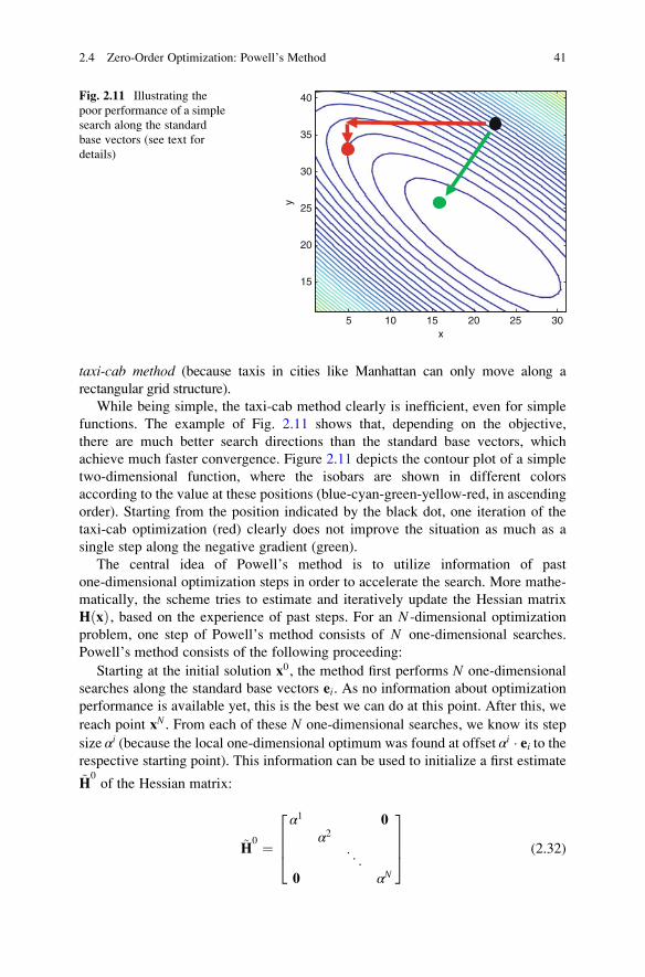
taxi-cab method (because taxis in cities like Manhattan can only move along a

rectangular grid structure).

While being simple, the taxi-cab method clearly is inefficient, even for simple

functions. The example of Fig. 2.11 shows that, depending on the objective,

there are much better search directions than the standard base vectors, which

achieve much faster convergence. Figure 2.11 depicts the contour plot of a simple

two-dimensional function, where the isobars are shown in different colors

according to the value at these positions (blue-cyan-green-yellow-red, in ascending

order). Starting from the position indicated by the black dot, one iteration of the

taxi-cab optimization (red) clearly does not improve the situation as much as a

single step along the negative gradient (green).

The central idea of Powell’s method is to utilize information of past

one-dimensional optimization steps in order to accelerate the search. More mathe-

matically, the scheme tries to estimate and iteratively update the Hessian matrix

H xð Þ, based on the experience of past steps. For an N -dimensional optimization

problem, one step of Powell’s method consists of N one-dimensional searches.

Powell’s method consists of the following proceeding:

Starting at the initial solution x0, the method first performs N one-dimensional

searches along the standard base vectors ei. As no information about optimization

performance is available yet, this is the best we can do at this point. After this, we

reach point xN . From each of these N one-dimensional searches, we know its step

size αi (because the local one-dimensional optimum was found at offset αi � ei to therespective starting point). This information can be used to initialize a first estimate

~H0of the Hessian matrix:

~H0 ¼

α1 0α2

. ..

0 αN

2664

3775 (2.32)

x

y

5 10 15 20 25 30

15

20

25

30

35

40Fig. 2.11 Illustrating the

poor performance of a simple

search along the standard

base vectors (see text for

details)

2.4 Zero-Order Optimization: Powell’s Method 41

Furthermore, a combined search direction can be calculated from the N steps by

setting sNþ1 ¼PN

i¼1αiei , which is equivalent to the sum of the columns of ~H

0. For

most kinds of functions f xð Þ , sNþ1 should be a much better search direction

compared to the ei . Consequently, we perform a one-dimensional search along

direction sNþ1 , thus reaching xNþ1 . Furthermore, we update ~H0by replacing one

column by sNþ1, yielding ~H1.

Now we can repeat N one-dimensional searches in the directions of the columns

of the current Hessian estimate ~H1, i.e., each of the N one-dimensional search

directions equals one column of ~H1. As a result, the position x2Nþ1 is reached. After

this, we can again calculate a combined search direction s2Nþ2, do a single search in

this direction, and update ~H1(reaching x2Nþ2 and obtaining ~H

2). This process can be

repeated until convergence is achieved. The entire proceeding can be summarized

in the following steps:

1. Initialization with a first successive search: PerformN one-dimensional searches

along the standard base vectors ei and estimate ~H0according to (2.32) yielding

the current solution estimate xN . Set k ¼ 0.

2. Search integration: Calculate s kþ1ð Þ� Nþ1ð Þ, where each element is the sum over all

columns of ~Hk(~hkjl denotes the element in the jth row and lth column of ~H

k):

skþ1ð Þ� Nþ1ð Þj ¼

X

l

~hkjl (2.33)

3. Combined search: Perform a single one-dimensional optimization in the direc-

tion of s kþ1ð Þ� Nþ1ð Þ yielding the current solution estimate x kþ1ð Þ� Nþ1ð Þ:

4. Update: Build ~Hkþ1

by replacing one column of ~Hkwith s kþ1ð Þ� Nþ1ð Þ:

5. Convergence check: Stop when the iteration slows down, e.g., when

x kþ1ð Þ� Nþ1ð Þ � xk Nþ1ð Þ�� ε; otherwise, increment k and go on with step 6.

6. Successive search: Perform N one-dimensional searches along the column

vectors of the current Hessian estimate ~Hk(yielding the current solution estimate

x kþ1ð Þ� Nþ1ð Þ�1) and go on with step 2.

One remaining question is which column of ~Hkis to be replaced by the average

search direction s kþ1ð Þ� Nþ1ð Þ in step 4. In the standard method, the first row of ~Hkis

replaced in each iteration step. A better choice, however, is to replace the column~hklmax

(with column index lmax), which specifies the search direction along which the

greatest decrease of f xð Þ (denoted by Δfmax ) occurred. This proceeding, which is

employed in the enhanced Powell method, is justified by the fact that column lmax has

a major influence when calculating the average search direction s kþ1ð Þ� Nþ1ð Þ and

therefore shouldn’t be considered twice.


This alleviates the drawback that, after a few iterations, the columns of ~Hktend to

become parallel and thus some directions are “lost,” as we cannot move toward these

directions any longer. As a consequence, the scheme might not converge anymore.

When replacing the direction being the most significant part of s kþ1ð Þ� Nþ1ð Þ, the trend

to linear dependency between the columns of ~Hkwill become less likely.

In addition to that, two checks are introduced after step 2 in the enhanced Powell

method. The combined search of step 3 is only performed if both checks are

positive. These two checks can be described as follows:

• The first check evaluates whether a further processing along the average search

direction s kþ1ð Þ� Nþ1ð Þ will actually be likely to improve the result. This is

considered to be true if the following condition holds:

f x kþ1ð Þ� Nþ1ð Þ�1 þ 2 � s kþ1ð Þ� Nþ1ð Þ�

< f x kþ1ð Þ� Nþ1ð Þ�1�

(2.34)

In detail, (2.34) evaluates whether the values of the function after considering

the extended average search direction (it is taken twice) are lower compared to the

function value at the current solution. If this is not the case, the assumption that the

average search direction represents a good direction for continuing the search is

supposed to be not true and, consequently, themethod proceeds directly with step 6.

• The second check helps ensuring that the columns of ~Hkwill be less likely to

become linear dependent. If the search direction ~hklmax, i.e., the direction in which

the greatest decrease Δfmax occurred during the last successive search, actually

contributes a major part to the total decrease of this last successive search, we

should replace ~hklmaxby the combined search direction in order to avoid linear

dependency (otherwise, this simply is not necessary). This can be considered to

be true if the following condition holds:

2 � fStart � 2 � fN þ fEð Þ � fStart � fN � Δfmaxð Þ2 < Δfmax � fStart � fEð Þ2 with

fE ¼ f x kþ1ð Þ� Nþ1ð Þ�1 þ 2 � s kþ1ð Þ� Nþ1ð Þ�

fN ¼ f x kþ1ð Þ� Nþ1ð Þ�1�

fStart ¼ f xk� Nþ1ð Þ�

(2.35)

Otherwise the method proceeds directly with step 6 (without performing the

average search and update of ~Hk). An overview of the method is given in the

flowchart of Fig. 2.12.

Some implementations of the method re-initialize the proceeding if no improve-

ment can be achieved in any direction employed in the successive search of step 6:

If none of the search directions ~hki ; i 2 1; 2; . . . ;N½ � yields a decrease of the function


f xð Þ, ~H is re-initialized with the standard base vectors ei and the method restarts with

step 1. Please note, however, that this case could also be a sign of convergence: if

we are sufficiently close to the minimum, no improvement can be made either.

Therefore, the algorithm has to deal with this as well.

Convergence criteria can be based on the displacement between solutions of

successive iteration steps (as stated above) or on the relative change of the function

values at these positions. In the second case, convergence is achieved if the

following inequality holds:

fStart � fNj j ε � fStartj j þ fNj jð Þ (2.36)

To sum it up, Powell’s method does not rely on an extensive analytical knowl-

edge of f xð Þ. Instead, it tries to improve its performance by incorporating knowl-

edge gathered in past optimization steps. Typically, this works well for problems up

to moderate dimension as well as for problems where there is not much coupling

between the individual variables to be minimized. In this case, the HessianH is near

diagonal.

In cases of several thousands of variables or if there is a strong coupling between

the variables (i.e.,H has many off-diagonal terms significantly differing from zero),

higher-order optimization methods usually perform better, i.e., need significantly

less function evaluations until convergence is achieved. However, please have in

mind that each function evaluation could be much more costly if the derivatives are

to be calculated as well. Consequently, Powell’s method could be an alternative if

the calculation and/or estimation of derivative information about f xð Þ is very time-

consuming.

Optimizationalong std.

base vectors

First approx. ofHessian H

∼ 0SCalculate com-bined search

dir.

Searchalong col.vec. of H

∼ k

Improvementwith combined

search ?

Convergence ?

no

no

yes

yesE

Combinedsearch

Update of H

∼ k

Fig. 2.12 Flowchart of the enhanced Powell method


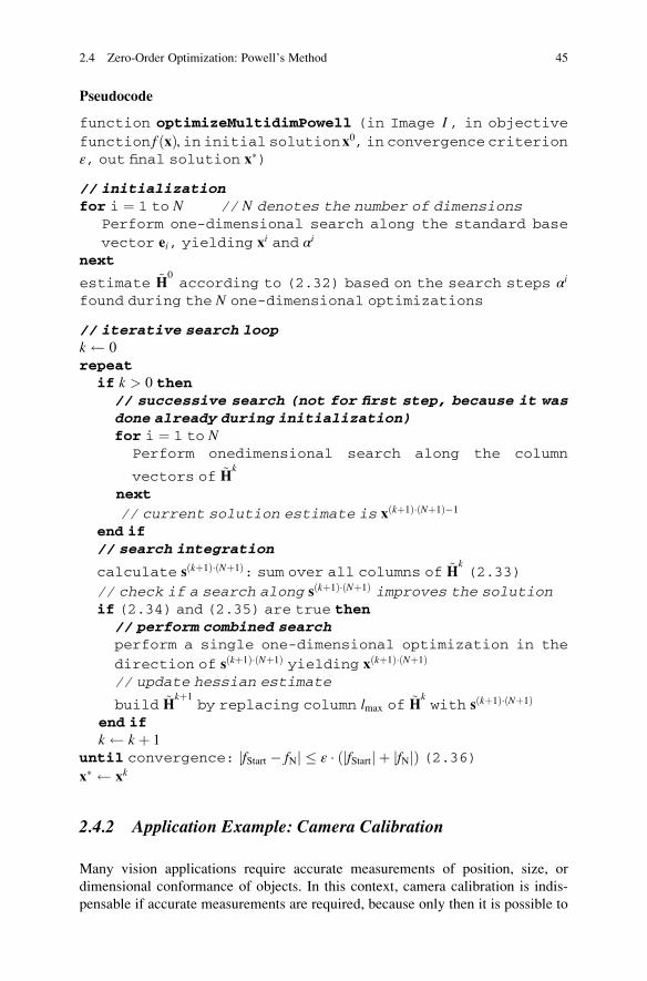
Pseudocode

function optimizeMultidimPowell (in Image I, in objective

function f xð Þ, in initial solutionx0, in convergence criterionε, out final solution x�)

// initializationfor i ¼ 1 to N // N denotes the number of dimensions

Perform one-dimensional search along the standard base

vector ei, yielding xi and αi

next

estimate ~H0according to (2.32) based on the search steps αi

found during the N one-dimensional optimizations

// iterative search loopk 0

repeatif k > 0 then

// successive search (not for first step, because it wasdone already during initialization)for i ¼ 1 to N

Perform onedimensional search along the column

vectors of ~Hk

next

// current solution estimate is x kþ1ð Þ� Nþ1ð Þ�1

end if// search integration

calculate s kþ1ð Þ� Nþ1ð Þ: sum over all columns of ~Hk(2.33)

// check if a search along s kþ1ð Þ� Nþ1ð Þ improves the solutionif (2.34) and (2.35) are true then

// perform combined searchperform a single one-dimensional optimization in the

direction of s kþ1ð Þ� Nþ1ð Þ yielding x kþ1ð Þ� Nþ1ð Þ

// update hessian estimate

build ~Hkþ1

by replacing column lmax of ~Hkwith s kþ1ð Þ� Nþ1ð Þ

end ifk k þ 1

until convergence: fStart � fNj j ε � fStartj j þ fNj jð Þ (2.36)x� xk

2.4.2 Application Example: Camera Calibration

Many vision applications require accurate measurements of position, size, or

dimensional conformance of objects. In this context, camera calibration is indis-

pensable if accurate measurements are required, because only then it is possible to


accurately infer metric values from pixel positions. In this section one example of

camera calibration, which utilizes Powell’s method, is presented. Observe that there

exist numerous applications requiring calibration of one or multiple cameras. The

book of Hartley and Zisserman [8] gives a good overview of this topic.

In many industrial applications, e.g., when inspecting manufactured objects, the

geometric setting of the camera relative to the objects to be measured can be chosen

such that simple conversions between metric and pixel values are possible. In a

frequently used setup, the camera axis is orthogonal to the object plane and the

distance between object and camera is fixed. Hence, if the sensor scale is known, it

should be possible to convert positions/sizes measured by the vision algorithm in

pixels into metric values in a simple fashion.

However, in practical applications, some imperfections usually occur. For

example, the optical properties of the lens usually include some imperfections.

Furthermore, it cannot be assured that the camera axis is perfectly orthogonal to the

object plane. Both effects reduce the accuracy of the system. Therefore, the

influence of these effects has to be quantified, which makes a correction of these

errors possible. This is done by modeling a transformation T between ideal and real

setup. Once T is known, we can apply T�1 for correction. To this end, camera

calibration has to estimate the coefficients of this transformation.

This is usually done by inspecting a calibration target, which is assured to be

manufactured very accurately and contains structures with known geometry, e.g.,

a regular grid of points with known pitch of the points (see, e.g., the upper right image

of Fig. 2.15, which depicts a camera image of a regular grid of points on a glass

calibration target). The coefficients are estimated by comparing measured positions

ui; vi½ � of the points to their nominal position xi; yi½ �, where the transformation u; v½ �¼ T x; y½ �ð Þ should be chosen such that the deviation (squared distance) E between

transformed and measured position becomes minimal (the vector t summarizes all

transformation coefficients):

t� ¼ argmintðEÞ ¼ argmin

t

X

i

ui; vi½ � � T xi; yi½ �; tð Þj j2 !

(2.37)

This is the point where optimization comes into play: optimization reveals the

desired parameters t� , which can be utilized for correction. In this example of

camera calibration, two effects are modeled:

• Perspective distortion: Here, rectangular structures are transformed into general

quadrangles, i.e., the angle between lines is not preserved (see Fig. 2.13). Such a

transformation is able to model out-of-plane rotation of the sensor chip of the

camera and hence the deviations between optical axis and object plane normal in

our case. Through the usage of so-called homogeneous coordinates (where the

2D positions are augmented by a third coordinate), this nonlinear relationship

can be modeled by a linear transform (see Fig. 2.13).


• Radial distortion: Typical lens imperfections result in a nonideal projection of

concentric circles. Each circle is projected to a circle again, but the diameter is

altered depending on the position of the circle with respect to the image center

(see equation in Fig. 2.14): the diameter of circles in the outer areas of the image

is mapped either too small (barrel distortion) or too large (pincushion distortion;

see Fig. 2.14).

If we combine both effects, each position xi; yi½ � is mapped to ui; vi½ � as follows(where xc; yc½ � is the center of the radial distortion):

uiðtÞ ¼ cos arctanp2;iðtÞp1;iðtÞ ��

� diðtÞ þ xc

viðtÞ ¼ sin arctanp2;iðtÞp1;iðtÞ ��

� diðtÞ þ yc

diðtÞ ¼ffiffiffiffiffiffiffiffiffiffiffiffiffiffiffiffiffiffiffiffiffiffiffiffiffiffiffiffiffiffiffiffiffip1;iðtÞ2 þ p2;iðtÞ2

q

1þ κ � p1;iðtÞ2 þ p2;iðtÞ2� with

p1;iðtÞ ¼ a11xi þ a12yi þ a13a31xi þ a32yi þ 1

� xc

p2;iðtÞ ¼ a21xi þ a22yi þ a23a31xi þ a32yi þ 1

� yc

(2.38)

The task of optimization here is to find a parameter vector parameter vector

t¼ a11; a12; a13; a21; a22; a23; a31; a32; κ; xc; yc½ � such that the sum of squared

11yx

a32a31

a23a22a21

a13a12a11

wvwuw

Fig. 2.13 Illustrating the effects of perspective transformation: generally, a rectangle is mapped

to a quadrangle (left). Using homogeneous coordinates, the transformation can be described by a

linear relationship (right)

21 ddd ′

Fig. 2.14 Illustrating the effects of radial distortion: here, circles are mapped to circles of different

diameter (left). The relationship between original and mapped diameter is stated in the middle. The

effect of radial distortion can be visualized with the help of rectangular point grids: the grid is

distorted especially in the image borders (right, with pincushion distortion)


deviations between measured and expected positions is minimized. This is a

classical nonlinear regression problem, where the Levenberg-Marquardt algorithm

could be used. However, to this end, derivative information of the transformation Twith respect to the parameter vector t ¼ a11; a12; a13; a21; a22; a23; a31; a32; κ; xc; yc½ �would be required. If we look at (2.38), it should be clear that this information is

difficult to be obtained. Therefore, Powell’s method seems suitable for a numerical

solution of (2.37).

The results of applying Powell’s method to this optimization can be seen in

Fig. 2.15: the upper left part depicts a camera image of the calibration target used,

which consists of a regular 11 � 11 grid of dark points. Usually the geometry of the

calibration target (particularly the spacing of the points) as well as the (mean)

sensor scale are known. Consequently, we can derive the expected pixel position

ui; vi½ � for each grid point from its corresponding position in metric coordinates

Fig. 2.15 Depicting some aspects of camera calibration (combination of perspective and radial

distortion) with Powell’s method: calibration target (upper left), calibration results (upper right),optimization details (lower left), and error analysis (lower right). See text for details


xi; yi½ �. A scheme detecting the dark circles reveals the actual positions ui; vi½ � in thecamera image. Hence, all input data needed for an application of Powell’s method

in order to reveal the transformation coefficients t is known.The overlaid circles shown in the upper right part of Fig. 2.15 illustrate the

optimization result: the green circles indicate the nominal position of each point,

whereas the red circles indicate the measured position (sometimes barely visible).

The blue circles show the estimated perspective part of the transformation, whereas

the orange circles indicate the entire transformation estimation (perspective+radial

distortion combined). Deviations of red, blue, and orange circles are magnified by a

constant factor for better visibility.

Ideally, the red and orange circles should coincide, if the estimated transforma-

tion parameters were able to perfectly model the distortion. As clearly can be seen,

the actual conditions come very close to this: most red circles are at least partly

shadowed by the orange ones (which relate to the estimated model), because their

positions are very close to each other.

This can also be seen in the lower right part of Fig. 2.15, where the deviation

between measured and nominal position of the points can be seen (y-axis),depending on the distance of the point to the image center (x-axis) before (red)

and after correction (green). Before correction, distortion is largest at positions far

away from the image center. After correction, the error at each point is virtually

independent from the distance and can be reduced by approximately one order of

magnitude here. These residual errors are mainly due to measurement accuracy

when estimating the actual position of each point, e.g., because of camera noise.

The course of a few parameters as optimization proceeds can be seen in the

upper left part of Fig. 2.15: here, the value of the objective function (red), the center

of radial distortion xc (green), and yc (blue) as well as the value of κ (yellow) are

shown for each calculation of (2.37). In total there are about 6,000 evaluations of

the objective function, with quite accurate results obtained after approximately

1,000 evaluations.

As far as performance is concerned, typical runtime of the optimization is about

200 ms on a notebook with a 2.2 GHz Intel Core i7 CPU (only one core is used).

2.5 First-Order Optimization

The methods presented so far utilize second-order derivatives of the objective

function (either explicitly or at least approximations) or no derivative information

at all. Instead of completely ignoring derivatives, there is something better we can

do, even if second-order information sometimes is difficult or impossible to be

obtained: we can take account of first-order information. The most simple way to

exploit first-order information is to take the negative gradient as search direction,

i.e., we can set sk ¼ �rf xk� �

. This simple proceeding, which is also known as

steepest descent method, is locally the best which can be done, because the negativegradient indicates the direction in which the function decreases fastest at the current

position. However, the actual rate of convergence can be quite poor in some

situations. In case of high curvature, e.g., the direction of fastest decrease might

change quite quickly if we move away from the current position.

2.5 First-Order Optimization 49

Nevertheless, the steepest descent is often used as initialization step of more

sophisticated methods. One of them, which is termed conjugate gradient method, ispresented in the following.

2.5.1 Conjugate Gradient Method

The conjugate gradient method (see, e.g., [13, 14]) picks search directions which

are conjugate to the search directions of the previous step. Two search directions siand sj are conjugate with respect to each other if the following relationship holds forsymmetric, positive definite matrices H:

sTi �H � sj ¼ 0 (2.39)

Why is picking conjugate search directions a good idea? In order to clarify this,

let’s assume that the objective function is anN-dimensional convex quadratic form,

e.g., f xð Þ ¼ 12� xT �H � x� aT � xþ c (where the N � N matrix H is symmetric and

positive definite). Now it can be shown that the minimum of this objective can be

found by successively performing line searches along the elements of a set of at

most N linearly independent search directions, which are mutually conjugate as

defined in (2.39). In other words, if we utilize “suitable” conjugate search

directions, we are able to find the minimum of a convex quadratic form in at

most N one-dimensional searches.

If we want to take gradient information into account, the best start is to perform a

steepest descent search, i.e., set s0 ¼ �rf x0ð Þ. Subsequent iterations now can try to

make use of the nice convergence properties of conjugate searches by searching

along directions which are conjugate with respect to the previous search direction.

The search direction of step k is calculated as follows:

sk ¼ �rf xk� �þ βksk�1

βk ¼ rf xk� �� 2

rf xk�1ð Þj j2(2.40)

Clearly, the current search direction sk is a combination of the direction of

steepest descent and the search direction of the last step. This utilization of

information about previous steps helps in improving the rate of convergence

(compared to steepest descent). As already said, this method is guaranteed to

converge in at most N steps for the special case of convex quadratic functions of

dimensionality N. For non-quadratic functions, however, of course more iterations

are necessary, but the expectation is that for those more general situations, the rate

of convergence is improved, too, at least as long the objective can be locally

approximated by a quadratic form sufficiently well.


The choice of βk as given in (2.40) ensures that sk and sk�1 are conjugate. It

was first proposed by Fletcher and Reeves, and that’s why the update rule in the

form of (2.40) is also known as Fletcher-Reeves method. Over the last decades,

many alternative rules for updating the βk aiming at increasing convergence

properties for non-quadratic objectives have been proposed (see, e.g., [7] for an

overview).

Observe, however, that the repeated application of (2.40) might result in numer-

ical ill-conditioning in some cases. In order to resolve numerical ill-conditioning,

two criteria can be applied. If one of them is fulfilled, the method can be restarted

with a steepest descent step. The resulting general proceeding can be seen in the

flowchart of Fig. 2.16.

In detail, these criteria are:

1. The one-dimensional search doesn’t improve the solution, i.e., f xk� �

> f xk�1� �

.

Please observe that this fact could also indicate that convergence is achieved.

Therefore, if a subsequent one-dimensional search in the direction of the steepest

descent doesn’t improve the search direction either, it is assumed that the

method has converged.

2. The slope of f with respect to the step size α of the general proceeding (see

Sect. 2.2) is positive: @f@α ¼ rf xk

� �; sk

� �> 0 (where �h i denotes the dot product

operator). This indicates numerical ill-conditioning. Consequently, the method

is restarted with steepest descent.

In general, this rather small modification compared to steepest descent results in

quite good rates of convergence. In particular, the conjugate gradient method is able

to follow “narrow valleys” of the objective rather quickly, whereas steepest descent

searches slow down in these situations.

Nevertheless, there exist other first-order methods trying to do better. For

example, in the so-called variable metric methods, information of previous steps

isn’t considered via a simple scalar β , but via an n-dimensional array, which is

capable of transporting more detailed information, of course. Examples of variable

metric methods are the Davidson-Fletcher-Powell algorithm (DFP) [14] or the

Broydon-Fletcher-Goldfarb-Shanno method (BFGS) [14].

noSet steepestdescent assearch dir.

1D-Optimizationin search dir.

S

E

yes

Convergence ?Ill-

conditioning ?

Set conjugategradient assearch dir.

no

yes

Fig. 2.16 Flowchart of the conjugate gradient method


Pseudocode

function optimizeMultidimConjugateGradient (in Image I, in

objective function f xð Þ , in initial solution x0, in conver-gence criterion ε, out final solution x�)

// initializazionk 0

bSteepestDescent true // calculate search directionaccording to steepest descent in the next iteration

// iterative main search looprepeat

if bSteepestDescent ¼¼ true then// set search direction to steepest descent

sk �rf xk� �

bSteepestDescent falseelse

// search direction is based on conjugate gradient

set search direction sk conjugate to the search directionof the last iteration according to (2.40)

end if

perform one-dimensional search along sk yielding xk

// check for ill-conditioning

if f xk� �

> f xk�1� �

|| rf xk� �

; sk� �

> 0 then

// ill-conditioning! restart with steepest descentbSteepestDescent true

if f xk� �

> f xk�1� �

&& f xk�1� �

> f xk�2� �

then

// no improvement could be made in two successiveiterations! convergence is achieved

x� xk

returnend if

end ifk k þ 1

until convergence: f xk� �� f xk�1

� �� ε � f xk� ��

x� xk

2.5.2 Application Example: Ball Inspection

Certain, mainly industrial, applications involve the usage of metal balls, e.g., ball

bearings, ball pens, or ball valves. In order to ensure proper functionality, it has to

be ensured that the ball shape is undamaged. Normally, this is done via dedicated


3D inspection systems (e.g., based on laser triangulation or structured light),

allowing for accurate 3D measurements. However, inspection with limited accu-

racy can also be performed with “conventional” 2D intensity images. If the position

of the balls has to be determined anyway, e.g., for gripping them during production,

a “conventional” camera system might already be in place. Inspection of the shape

can then be done without additional hardware.

Consider a scenario where the camera axis is perpendicular to the object plane

and the images of the ball(s) to be inspected are taken with slanted illumination. As

the mostly shiny surface of the metal balls leads to mainly direct reflections of the

incident light, the balls appear as bright rings in the grayscale camera image, where

the ring diameter depends on the slant angle.

This is illustrated in Fig. 2.17. The left part illustrates the reflectance model of

mostly shiny surfaces like polished metal. For those materials direct reflections

dominate (the dashed lines indicate reflected light and the thickness indicates

illumination strength). Applied to ball-shaped objects (right picture of Fig. 2.17),

we can see that only a small range of surface orientations leads to reflections into

the sensor chip (blue), in case the ball is illuminated from the side (indicated by

solid lines). Due to the ball shape, the surface patches with “correct” orientation are

arranged as a ring. Consequently, the ball appears as a bright ring with slanted

illumination, where the diameter depends on the slant angle.

Inspection can then be fulfilled by designing a parametric model for the bright-

ness appearance of a ball in the camera image (which should take the shape of a

ring) and then fitting this model to the camera image showing a particular ball to

inspect. This fitting represents an optimization task, which can be accomplished

with the method just presented above, as we will see shortly. During optimization,

the parameters of the model are optimized such that they best represent the image.

Subsequently, the optimization result can be used twofold for inspection:

• First, it can be checked whether the estimated model parameters are within the

expected range.

• Second, the difference between the optimized model and the ball appearance in

the camera image (which is the value of the objective function after convergence

of the optimization algorithm) has to remain below a certain threshold; other-

wise, the ball features a deformation which is too large.

a

a

Fig. 2.17 Illustrating the reflectance properties of mostly shiny reflections (left), where the main

part of the light from the object surface is a direct reflection of the incoming light. Consequently,

ball-shaped objects appear as bright rings with slanted illumination, as the reflected light hits the

sensor only if the surface patch has a specific normal angle (right, sensor in blue)


An appropriate model M of a bright ring is a radially shifted two-dimensional

Gaussian, which can be expressed in Cartesian coordinates by

M x; yð Þ ¼ oþ m � exp �ffiffiffiffiffiffiffiffiffiffiffiffiffiffiffiffiffiffiffiffiffiffiffiffiffiffiffiffiffiffiffiffiffiffiffiffiffiffiffiffiffix� xcð Þ2 þ y� ycð Þ2

q� r

a

0@

1A

2264

375 (2.41)

where x; y½ � represents the pixel coordinate, xc; yc½ � the center of the ring, r and a itsradius and width, o the brightness offset, and m the intensity magnitude of the ring

(see Fig. 2.18).

The objective function can be defined as the sum of the squared differences

between observed image data and the model in a local neighborhood where the

ball is expected:

F xð Þ ¼X

x;y2NI x; yð Þ �M x; y; xð Þ½ �2 (2.42)

where I x; yð Þ denotes the intensity of the camera image at position x; y½ �, defines

the neighborhood for which camera image and model are to be compared, and

x¼ xc; yc; r; a;m; o½ �T is the vector containing the design variables of the model to

be optimized. Hence, we end up with a six-dimensional continuous optimization

problem.

In order to improve convergence, we can also consider derivative information

during the optimization process. By repeatedly applying the chain rule, the partial

derivatives of F xð Þwith respect to the model parameters are (for convenience, let’s

introduce d ¼ffiffiffiffiffiffiffiffiffiffiffiffiffiffiffiffiffiffiffiffiffiffiffiffiffiffiffiffiffiffiffiffiffiffiffiffiffiffiffiffiffix� xcð Þ2 þ y� ycð Þ2

qand k ¼ � d � rð Þ a=ð Þ2):

Fig. 2.18 Depicting a 3D

plot of the circular ring

brightness model of (2.41)


@F xð Þ@xc

¼X

x;y2N2M x; yð Þ � 2I x; yð Þð Þ � m � ek � 2 x� xcð Þ

a21� r

d

� ��

@F xð Þ@yc

¼X

x;y2N2M x; yð Þ � 2I x; yð Þð Þ � m � ek � 2 y� ycð Þ

a21� r

d

� ��

@F xð Þ@r

¼X

x;y2N2M x; yð Þ � 2I x; yð Þð Þ � m � ek � � 2r � 2d

a2

��

@F xð Þ@a

¼X

x;y2N2M x; yð Þ � 2I x; yð Þð Þ � m � ek � � 2 d � rð Þ2

a3

!" #

@F xð Þ@m

¼X

x;y2N2M x; yð Þ � 2I x; yð Þð Þ � ek� �

@F xð Þ@o

¼X

x;y2N2M x; yð Þ � 2I x; yð Þ½ �

(2.43)

When regarding the first derivatives of (2.43), it is evident that it would be very

cumbersome to derive second-order information analytically (apart from the compu-

tational effort to calculate the Hessian numerically in each iteration step). Conse-

quently, only first-order derivative information shall be considered during

optimization and the conjugate gradient method is chosen in order to minimize F xð Þ.Now each ball can be checked individually for deformations. Figure 2.19 shows

two example balls where the images were taken with flat illumination: a good ball

(top row) and a bad ball (bottom row). In the top row the model approximates the

image region very well (small differences for all pixels; see right column). Com-

pared to that, the bottom row reveals that the ring diameter is larger (r too large), itsthickness is slightly smaller (small a), and, additionally, there are more pixels with

significant brightness difference between optimized model and camera image,

especially in the right region of the ring as well as within the region composed of

the ball center (right column: similar brightness is indicated by gray pixels).

This inspection can be performed for multiple slant angles, where each slant

angle could reveal ball deformations on different parts of the ball surface. Clearly,

this method is not as powerful as dedicated 3D surface inspection, but it is

economical and quite capable of detecting major deformations.

2.5.3 Stochastic Steepest Descent and Simulated Annealing

2.5.3.1 General Proceeding

A special case of objective functions which can be found quite often in practice is

characterized by the fact that the objective function can be written as a sum of Nelements:


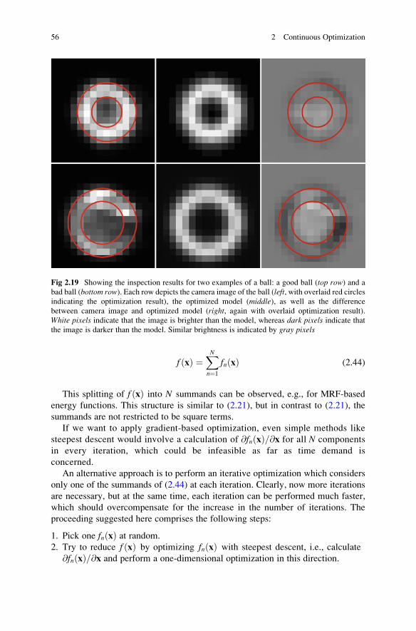
f xð Þ ¼XN

n¼1fn xð Þ (2.44)

This splitting of f xð Þ into N summands can be observed, e.g., for MRF-based

energy functions. This structure is similar to (2.21), but in contrast to (2.21), the

summands are not restricted to be square terms.

If we want to apply gradient-based optimization, even simple methods like

steepest descent would involve a calculation of @fn xð Þ @= x for all N components

in every iteration, which could be infeasible as far as time demand is

concerned.

An alternative approach is to perform an iterative optimization which considers

only one of the summands of (2.44) at each iteration. Clearly, now more iterations

are necessary, but at the same time, each iteration can be performed much faster,

which should overcompensate for the increase in the number of iterations. The

proceeding suggested here comprises the following steps:

1. Pick one fn xð Þ at random.

2. Try to reduce f xð Þ by optimizing fn xð Þ with steepest descent, i.e., calculate

@fn xð Þ @= x and perform a one-dimensional optimization in this direction.

Fig 2.19 Showing the inspection results for two examples of a ball: a good ball (top row) and a

bad ball (bottom row). Each row depicts the camera image of the ball (left, with overlaid red circlesindicating the optimization result), the optimized model (middle), as well as the difference

between camera image and optimized model (right, again with overlaid optimization result).

White pixels indicate that the image is brighter than the model, whereas dark pixels indicate thatthe image is darker than the model. Similar brightness is indicated by gray pixels


Now, the derivative calculation should be rather simple at each step. The

procedure is repeated until convergence, e.g., the reduction of f xð Þ is sufficientlysmall. This proceeding is called stochastic steepest descent (or stochastic gradientdescent) and is an example of a so-called greedy algorithm, as each iteration seeks

to maximize the reduction of f xð Þ.The main drawback of this proceeding (like any local method presented in this

chapter) is its susceptibility to get trapped in a local minimum if the objective

function is not convex. A method to overcome this problem is to allow for updates

of the solution which actually increase to objective function with a certain proba-

bility. Then it should be possible to escape local minima.

Rather than minimizing fn xð Þ at each step, we can select a certain state x with

probabilityp xð Þ / exp �fn xð Þ T=½ �. For most of the time,x is modified such that fn xð Þis reduced (because then p xð Þ takes a rather high value, which makes xmore likely

to be selected), but sometimes states are chosen where the fn xð Þ is actually

increased, enabling the algorithm to get away from a local minimum. High values

ofT lead to rather random updates, whereas low values ofT effect in a quick decline

in p xð Þ for high energy states and therefore strongly bias updates which reduce the

objective.

In an approach called simulated annealing, stochastic gradient descent is

performed with high T at start, and T is gradually lowered (“annealed”) as iteration

proceeds (see [9]). Simulated annealing was the method of choice for a long time

for applications where local minima trapping is an issue. In the meantime, however,

more powerful methods, which have proven to outperform simulated annealing in

many situations, emerged. Especially to mention here are so-called graph cuts,

which will be presented in Chap. 7.

2.5.3.2 Example: Classified Training for Object Class Recognition

Vijnhoven et al. [15] showed how stochastic gradient descent optimization can be

successfully applied to the task of training a decision function for object detection.

They considered the application of detecting instances of a certain object category,

e.g., “cars” or “pedestrians,” in an image, which can be solved by the approach

suggested in [4].

Dalal et al. derive a feature vector d (a so-called descriptor) which they call

“Histograms of Oriented Gradients” (HOG) from a subregion of the image and,

based ond, run a classifier which decides whether an instance of the object categoryto be searched is present at this particular position or not. The classifier has a binary

output: -1 for “object not present” and 1 for “object present.” In order to scan the

image, they propose a so-called sliding window approach, where the region for

calculating the descriptor is shifted pixel by pixel over the entire image, with a

subsequent classification at every position. Finally, they obtain a position vector

where each element reveals the position of a detected instance of the searched

object category.


http://dx.doi.org/10.1007/978-1-4471-5283-5_7

The classifier has to be trained prior to recognition in an off-line teaching phase

with the help of example images. A Support Vector Machine (SVM) for classifica-

tion is used in [4], whereas the authors of [15] suggest to employ SGD in the

classifier training step. Through the usage of SGD, they showed to reduce training

times by a factor of 100–1,000 with similar recognition performance.

Before we describe in detail how SGD is utilized in training, let’s first take a closer

look at some different aspects of the proceeding of [4] (HOG descriptor, sliding

window, and classifier design) in order to get a better understanding of the method.

HOG Descriptor

Similar to the well-known SIFT descriptor (see [11]), the HOG descriptor proposed

by Dalal et al. accumulates intensity gradient orientations into histograms. To this

end, the area of interest is partitioned into small “cells,” e.g., of 8 � 8 pixel in size

(see Fig. 2.20). Now, within each cell, a histogram of gradient orientation is

calculated, i.e., the range of possible orientations (0�–360� if we want to consider

gradient sign) is partitioned into a certain number of bins (typically 10–20 bins are

used), and each pixel votes for the bin which corresponds to its gradient orientation

(see Fig. 2.20). The vote can be provided with a weight, e.g., according to gradient

magnitude and/or distance between the pixel and a block center (see below).

This proceeding leads to a considerable invariance of the resulting descriptor

with respect to typical variations occurring when acquiring images of different

instances of the object class to be detected, such as varying illumination, small

deformations, and viewpoint change. The usage of gradient orientations makes the

descriptor robust with respect to illumination changes, whereas the rather loose

spatial pooling of pixels into cells increases the invariance with respect to spatial

variations, like local deformations and viewpoint change.

Additionally, neighboring cells can be combined to one so-called block, e.g.,

2 � 2 cells form one block. Within each block, a local contrast normalization is

performed in order to compensate for illumination variance or effects like

shadowing. To this end, the block descriptor vector is normalized with respect to

some vector norm. In [4] it was reported that histogram sizes of 18 bins give good

results; therefore, a block consisting of 2 � 2 cells results in a descriptor of size 72.

This process of computing normalized descriptors for a block is repeated for all

blocks of the area of interest. Note that recognition performs best if overlapping

blocks are used. To this end, neighboring blocks are shifted by only one cell with

respect to each other, i.e., they share some cells (cf. Fig. 2.20). The descriptors of all

blocks being part of the area of interest are concatenated into one common

descriptor vector d, which now is a robust representation of the area of interest.

The overlapped calculation may seem to be redundant, but Dalal et al. showed that

accurate local contrast normalization is crucial for good performance and

overlapping helps to achieve this.


Sliding Window

During recognition, a “dense” calculation of the HOG descriptor is performed,

i.e., the window of pixels which contribute to the descriptor is shifted densely, e.g.,

by just one pixel, and after each shift a new descriptor is calculated. Each

HOG descriptor can be used as input for a binary classification, which outputs

“object present” or “no object present” for a particular descriptor/position. This

dense evaluation is in contrast to other descriptor-based approaches for object

detection (like the usage of SIFT descriptors as proposed in [11]), which

Fig. 2.20 Indicating the flow of the calculation of a HOG descriptor: after gradient calculation,

the detection window is partitioned into cells, and within each cell a 1D histogram of gradient

orientations is calculated. Several cells are pooled into a block, and a local normalization step is

performed for all cells of the block. The final feature vector consists of the information of all

blocks in the detection window, whereas the blocks spatially overlap (From Dalal and Triggs [4],

with kind permission)


concentrate on interest points and therefore are “sparse.” A dense calculation is

more time-consuming but at the same time considers more information, which

increases recognition performance.

Classification

For the classification being performed at each position of the dense sampling grid,

a linear classifier is used, i.e., the decision function c dð Þ is a weighted sum of the

elements of the feature vector d:

c dð Þ ¼ wT � dþ b (2.45)

where w is a vector of weights and b is a bias. Values of c dð Þ > 0 indicate the

presence of an object instance. The weights w and b are to be trained in a training

phase, which is performed “off-line” prior to recognition based on a database of

training images showing the object class to be detected.

The goal of the training step is to determine the weights w� and bias b� whichyields best classification performance if applied to the set of training samples,

which consists of N images. Optimal parameters w� and b� can now be found

with a stochastic gradient descent method, as shown in [15].

To this end, a HOG descriptor dn; n 2 1; 2; 3; . . . ;Nf g is calculated for each

training image. We need a supervised training here, which means that a label ln2 �1; 1f g is assigned to each training image by a supervisor, depending on whether

the image contains an instance of the object class to be searched or not.

For each training image, we can apply the linear classifier to its HOG descriptor.

As a result, we get an estimation ln for its label: ln ¼ wT � dn þ b. The difference

between the user annotation ln and its estimation ln can be used to define a loss

function En, which should be small if there is a small discrepancy between ln and lnand large if ln differs significantly from ln

En ¼ max 0; 1� ln � wTdn þ b� ��

(2.46)

The performance of a particular classifier can be measured by the total loss for

the entire training set, which is based on a sum of the losses of each individual

training sample:

E ¼ λ

2� wk k2 þ 1

N

XN

n¼1En ln; ln� �

(2.47)

where wk k is a regularization term and λ determines the relative weighting between

the regularization term and the correctness of classification. Without using a

regularizer there would be the danger that the optimization gives extremely high

weights to just a small fraction of the examples which can easily be classified

correctly and therefore ignores poor classification performance of a possibly large

number of examples with small weights.


With the help of a minimization of the energy function defined in (2.47), we can

determine the weight vector w� and bias b� which yield the best partitioning of the

training set (into “object” or “no object” classes).

Standard gradient descent now would require to compute all partial derivatives

@En @w= with respect to w and optimize the entire sum of (2.47) taking all training

examples into account at each one-dimensional step. Typically, this joint

one-dimensional optimization of E is computationally expensive or even infeasible

even for training sets of moderate size.

At this point, stochastic gradient descent comes into play. Here,w is also updated

iteratively, but now the update is performed based on just one training sample at

each iteration. Taking just one @En @w= into account yields the following update

formula:

wtþ1 ¼ wt � η

t� @En

@wt

¼ wt � ηt � λwt þ@En ln wT

t dn þ b� ��

@wt

�with ηt ¼

1

λ � tþ t0ð Þ ð2:48Þ

where the parameters λ and t0 have to be chosen by the user. At each iteration step t,one training sample n is picked at random, until all training images are used. In [15]

training is performed in just one sweep (i.e., the optimization with respect to each

training sample is performed exactly once), but it is also conceivable to do multiple

sweeps.

Experimental results provided in [15] for the object class “car” indicate that,

compared to the standard SVM implementation of the HOG scheme, SGD has the

following advantages:

• Training can be sped up by two to three orders of magnitude, depending on the

particular SVM implementation.

• A slight increase in recognition performance can be reported for some object

classes. In order to get an impression about the performance of the scheme,

Fig. 2.21 shows detection results for several challenging scenes for the object

class “car”. Red frames indicate wrong detections and green frames correct ones

(with a significantly large overlap between detected area and ground truth).

• The nature of the training algorithm admits online training, because we can do an

extra iteration of the SGD training step at any time, e.g., when some new

samples (which should help to improve classification performance) become

available.

2.6 Constrained Optimization

For the methods presented up to now, the only criterion when calculating the

solution x� is to minimize the objective f xð Þ. In many applications, however, x�

has to fulfill additional requirements. More specifically, the range of values each

2.6 Constrained Optimization 61

element of x� can take might be constrained. In other words, the solution space S isconstrained to some subspace of Rn . For example, when calibrating a camera as

proposed in Sect. 2.4.2, a reasonable assumption is that the center of the radial

distortion is located within the image.

Of course, such constraints (if existent) have to be considered when calculating

the solution. The field dealing with these additional requirements is called

constrained optimization. Due to space reasons, we don’t give an exhaustive

treatment of this topic and just present some important ideas on how to consider

additional constraints. The interested reader is referred to, e.g., [3] for a more

detailed introduction.

First, we have to note that there are two types of constraints. The first type is

called equality constraint, because here some function of the elements of x� has tobe exactly equal to some constant value. Mathematically, this can be expressed by

gm xð Þ ¼ 0 with m 2 1; 2; . . . ;M½ � (2.49)

Fig. 2.21 Illustrating the recognition performance of a HOG detector for cars when trained with

stochastic gradient descent. Correct detections are boxed by a green rectangle and false

classifications by a red one. As clearly can be seen, the algorithm shows good performance,

even if the appearance of the cars varies significantly (© 2010 IEEE. Reprinted, with permission,

from Vijnhoven and de Width [15])


where each gm describes a separate constraint. Another type of constraints are the

so-called inequality constraints, where some function hn xð Þ is restricted to take

values which are constrained by an upper bound:

hn xð Þ 0 with n 2 1; 2; . . . ;N½ � (2.50)

A simple example for both types of constraints is given in Fig. 2.22 in the case of a

two-dimensional solution space, where in the left illustration the solution is

constrained to be located on a circle of radius r (i.e., x21 þ x22 ¼ r), which is an equalityconstraint. The right image depicts a situation where the solution has to be located

inside some circle (i.e., x21 þ x22 r), which is an example of an inequality constraint.

In the following, some ideas on how to consider these constraints are given. In

the following, the schemes dealing with constraints are categorized into three

categories:

• Projection methods

• Penalty methods

• Barrier methods

The main idea of so-called projection methods is to first calculate the solution

update with some iterative method as described previously as in the unconstrained

case and then project back this update to a “valid” position which meets the

constraints. This back-projection is done at the end of each iteration.

A particularly simple proceeding can be performed if each element of x is

constrained to be within a certain range of values, i.e., xi;l xi xi;u. Then we can

simply set xki to xi;l if it is below this threshold, and, respectively, to xi;u if is largerthan xi;u . After this correction step, the iteration can proceed analogously to the

unconstrained case.

The back-projection can be integrated very well into iterative the methods

presented in the previous chapters. The only modification compared to the uncon-

strained case is to perform the additional back-projection step at the end of each

iteration.

Different from this, penalty methods aim at modifying the objective f xð Þ suchthat solutions located far away from the constrained solution space are penalized

r

x1

x2

r

x1

x2

Fig. 2.22 Illustrating the different types of constraints for a two-dimensional example: in the leftfigure, the solution space is restricted to a circle with radius r (equality constraint), whereas in the

right figure the interior of the circle is part of the solution space, too (inequality constraint)

2.6 Constrained Optimization 63

and therefore avoided by the optimization algorithm. To this end, a penalty term is

introduced in the objective:

p xð Þ ¼ f xð Þ þ c �XM

m¼1gm xð Þ2 þ

XN

n¼1max 0; hn xð Þ2

� " #(2.51)

The modified objective p xð Þ can now be optimized with any unconstrained

optimization method. However, please note that there is no guarantee that all

constraints are actually met by the found solution, violations of the constraints

just become less likely. Therefore, the whole process is performed iteratively,

where in each iteration l , the weight cl of the influence of the penalty term is

increased successively in order to be sure that the constraints are met at finish.

Observe that here one iteration comprises the application of the complete proceed-

ing of an unconstrained optimization method.

Similar to that, the so-called barrier methods (also termed interior methods)modify the objective function through the introduction of a penalty term, too.

Additionally, they assume that the optimization starts within the constrained

solution space and hence can only be applied to problems with inequality

constraints. The penalty term should introduce costs getting larger when we

approach the border of the constrained solution space. This can be formulated as

b xð Þ ¼ f xð Þ � c �XN

n¼1

1

hn xð Þ (2.52)

As each hn xð Þ 0, this actually introduces costs. These additional costs aim at

ensuring that the constrained solution space is never left. Observe that the hn can

always be designed to take nonpositive values by multiplication with �1, if

necessary.

Again, b xð Þ can be optimized through the iterative application of an uncon-

strained optimization method. This time, however, the cl is successively reduced,

which means that the constraints are loosened if we already are near the optimum in

order to get more accurate results.

References

1. Bjorck A (1996) Numerical methods for least squares problems. Society for Industrial and

Applied Mathematics, Philadelphia. ISBN 978-0-898-71360-2

2. Bonnans J-F, Gilbert JC, Lemarechal C, Sagastizabal CA (2006) Numerical optimization –

theoretical and practical aspects, 2nd edn. Springer, Berlin\New York. ISBN 978-3-540-

35445-1

3. Boyd S, Vandenberghe L (2004) Convex optimization, 2nd edn. Cambridge University Press,

Cambridge\New York. ISBN 978-0-521-83378-3

4. Dalal N, Triggs B (2005) Histograms of oriented gradients for human detection. Comput Vis

Pattern Recognit 1:886–893


5. Domokos C, Nemeth J, Kato Z (2012) Nonlinear shape registration without correspondences.


6. Golub GH, Van Loan CF (1996) Matrix computations, 3rd edn. Johns Hopkins University

Press, Baltimore. ISBN 0-8018-5414-8

7. Hager WW, Zhang H (2006) A survey of nonlinear conjugate gradient methods. Pac J Optimiz

2(1):35–58

8. Hartley R, Zisserman A (2004) Multiple view geometry in computer vision, 2nd edn.

Cambridge University Press, Cambridge. ISBN 978–0521540513

9. Kirkpatrick S, Gelatt CD, Vecchi MP (1983) Optimization by simulated annealing. Science

220(4598):671–680

10. Levenberg K (1944) A method for the solution of certain non-linear problems in least squares.

Q Appl Math 2:164–168

11. Lowe DG (2004) Distinctive image features from scale-invariant viewpoints. Int J Comput Vis

60:91–111

12. Marquardt D (1963) An algorithm for least-squares estimation of nonlinear parameters. SIAM

J Appl Math 11(2):431–441

13. Shewchuck JR (1994) An introduction to the conjugate gradient method without the agonizing

pain. Technical Report Carnegie Mellon University, Pittsburgh

14. Vanderplaats GN (1984) Numerical optimization techniques for engineering design. McGraw

Hill, New York. ISBN 0-07-066964-3

15. Vijnhoven R, de Width P (2010) Fast training of object detection using stochastic gradient

descent. In: 20th international conference on pattern recognition, Washington DC. pp 424–427

References 65

Chapter 3

Linear Programming and the SimplexMethod

Abstract Problems where the objective function to be optimized is linear in its

design variables are of particular interest, because then a solution can be found

very efficiently. Solutions of linear objective functions can only be unique if

additional constraints exist. While the constraints bound the solution space, the

linear nature of the objective ensures that the solution must be located at

the border of this bounded solution space. In the case of linear constraints, the

bounded solution space has the form of a polyhedron, and, hence, it suffices to

seek for the solution at the vertices of the bounded space. As a consequence, the

optimum can be found very fast. One method for solving linear programs is the

simplex algorithm, which is one of the most famous optimization algorithms. It

identifies the solution by moving from a vertex to one of its neighbors until the

value of the objective cannot be reduced further for all neighboring vertices. In

order to benefit from the speed advantage of linear programming, it sometimes

is promising to approximate a given problem by linear relationships. Such an

approximation is presented for the task of stereo disparity estimation at the end

of this chapter.

3.1 Linear Programming (LP)

As already stated above, a special case of continuous optimization occurs when the

objective function is linear in all its variables, i.e.,

f xð Þ ¼ c1x1 þ c2x2 þ � � � þ cNxN ¼XN

i¼1

cixi ¼ cT � x (3.1)

Please note that this function has no local minima, as all derivatives are nonzeroover the entire solution space: @f xð Þ @xi ¼ ci 6¼ 0 8 i 2 1; . . . ;N½ �= . Please note that

it can be assumed that all ci ’s are nonzero, because if a specific ci was zero, theobjective function would be independent of xi , and, consequently, no optimization



67

would be possible for this design variable. Consequently, if the solution space is

unbounded, no solution exists (as it would be located at some point in infinity).

Hence, a solution can only be obtained if additional constraints are introduced:

XN

i¼1

aji xi � bj or; equivalently; aTj � x � bj; j 2 1; . . . ;M½ � (3.2)

If the sum on the left-hand side has to be exactly equal to bj , we talk about

an equality constraint; otherwise, the constraint is termed an inequality constraint.M denotes the number of constraints which exist for a given problem.

Observe that all constraints of the form of (3.2) are linear in the design variables,

too. A situation where not only the objective function but also the constraints are

linear in all design variables is called a linear program (LP) .

A graphical interpretation of linear programs is that all contour lines, where f xð Þtakes the same value, are straight lines. The constraints are also represented by

straight lines. This can be shown with the help of a two-dimensional example:

consider the objective function f xð Þ ¼ 3 � x1 � 1:5 � x2, which is represented by its

contour lines in Fig. 3.1. The colors of the contour lines indicate the value of the

objective at a particular position. Here, the standard MATLAB color palette is used

(red-orange-yellow-cyan-blue-dark blue, in decreasing order). Suppose that each

design variable is limited to nonnegative values (limits are indicated by the black

coordinate axes). After introducing two additional constraints � 0:3 � x1 þ x2 � 5

(indicated by the thick red line) and 6:25 � x1 þ x2 � 50 (thick blue line), the

solution space is bounded by a quadrangle consisting of segments of the constraints.

Considering the extension to N-dimensional problems, the solution set becomes a

convex polyhedron.

x

y

−1 0 1 2 3 4 5 6 7 8 9 10−1

0

1

2

3

4

5

6

7

8

9


solution set of a

two-dimensional objective

function, which is restricted

by several constraints

68 3 Linear Programming and the Simplex Method

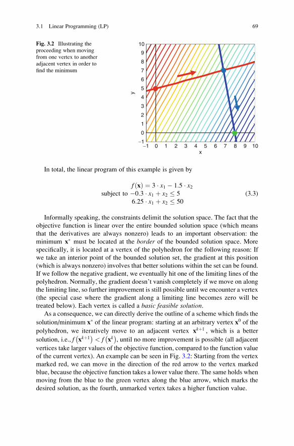
In total, the linear program of this example is given by

subject to

f xð Þ ¼ 3 � x1 � 1:5 � x2�0:3 � x1 þ x2 � 5

6:25 � x1 þ x2 � 50

(3.3)

Informally speaking, the constraints delimit the solution space. The fact that the

objective function is linear over the entire bounded solution space (which means

that the derivatives are always nonzero) leads to an important observation: the

minimum x� must be located at the border of the bounded solution space. More

specifically, it is located at a vertex of the polyhedron for the following reason: If

we take an interior point of the bounded solution set, the gradient at this position

(which is always nonzero) involves that better solutions within the set can be found.

If we follow the negative gradient, we eventually hit one of the limiting lines of the

polyhedron. Normally, the gradient doesn’t vanish completely if we move on along

the limiting line, so further improvement is still possible until we encounter a vertex

(the special case where the gradient along a limiting line becomes zero will be

treated below). Each vertex is called a basic feasible solution.As a consequence, we can directly derive the outline of a scheme which finds the

solution/minimum x� of the linear program: starting at an arbitrary vertex x0 of the

polyhedron, we iteratively move to an adjacent vertex xkþ1 , which is a better

solution, i.e., f xkþ1� �

< f xk� �

, until no more improvement is possible (all adjacent

vertices take larger values of the objective function, compared to the function value

of the current vertex). An example can be seen in Fig. 3.2: Starting from the vertex

marked red, we can move in the direction of the red arrow to the vertex marked

blue, because the objective function takes a lower value there. The same holds when

moving from the blue to the green vertex along the blue arrow, which marks the

desired solution, as the fourth, unmarked vertex takes a higher function value.

x

y

−1 0 1 2 3 4 5 6 7 8 9 10−1

0

1

2

3

4

5

6

7

8

9


proceeding when moving

from one vertex to another

adjacent vertex in order to

find the minimum

3.1 Linear Programming (LP) 69

Please note that the minimum was found in just two iterations. This observation

gives a hint why linear programs are so attractive: the fact that the solution (if

existent) must lie at the border of the constrained solution set enables us to find it

very quickly. Consequently, many researchers try to describe or approximate their

problem at hand by a linear program.

However, the existence of a unique solution is not guaranteed. Actually, four

types of solution exist for linear programs, depending on the constraints:

1. Unique solution: Here, the constraints ensure that the solution set is entirely

bounded. This case is shown in the left picture of the upper row of Fig. 3.3 (the

solution set is indicated by the ruled area). The solution is located at a vertex of

the polyhedron bounding the solution set.

2. Non-unique solution: As in case (1), the constraints entirely bound the solution

set. In contrast to case (1), however, one of the lines indicating the constraints is

parallel to the contour lines. Consequently, the objective function takes the same

value at each position of the “constraint line”. If the value of the objective

function along this line is minimal for the constrained set, there exist multiple

x

y

-1 0 1 2 3 4 5 6 7 8 9 10-10123456789

10

y

y

-1 0 1 2 3 4 5 6 7 8 9 10-10123456789

10

x

y

-1 0 1 2 3 4 5 6 7 8 9 10-10123456789

10

x

y

-1 0 1 2 3 4 5 6 7 8 9 10-10123456789

10

Fig. 3.3 Depicting the solution set for different cases (see text for details)


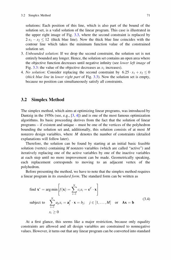
solutions: Each position of this line, which is also part of the bound of the

solution set, is a valid solution of the linear program. This case is illustrated in

the upper right image of Fig. 3.3, where the second constraint is replaced by

2�x1 � x2 � 12 (thick blue line). Now the thick blue line coincides with the

contour line which takes the minimum function value of the constrained

solution set.

3. Unbounded solution: If we drop the second constraint, the solution set is not

entirely bounded any longer. Hence, the solution set contains an open area where

the objective function decreases until negative infinity (see lower left image of

Fig. 3.3: the value of the objective decreases as x1 increases).4. No solution: Consider replacing the second constraint by 6:25 � x1 þ x2 � 0

(thick blue line in lower right part of Fig. 3.3). Now the solution set is empty,

because no position can simultaneously satisfy all constraints.

3.2 Simplex Method

The simplex method, which aims at optimizing linear programs, was introduced by

Dantzig in the 1950s (see, e.g., [3, 4]) and is one of the most famous optimization

algorithms. Its basic proceeding derives from the fact that the solution of linear

programs – if existent and unique – must be one of the vertices of the polyhedron

bounding the solution set and, additionally, this solution consists of at most Mnonzero design variables, where M denotes the number of constraints (detailed

explanations will follow later).

Therefore, the solution can be found by starting at an initial basic feasible

solution (vertex) containing M nonzero variables (which are called “active”) and

iteratively replacing one of the active variables by one of the inactive variables

at each step until no more improvement can be made. Geometrically speaking,

each replacement corresponds to moving to an adjacent vertex of the

polyhedron.

Before presenting the method, we have to note that the simplex method requires

a linear program in its standard form. The standard form can be written as

find x� ¼ argmin f xð Þ ¼XN

i¼1

cixi ¼ cT � x" #

subject toXN

i¼1

ajixi ¼ aTj � x ¼ bj; j 2 1; . . . ;M½ � or Ax ¼ b

xi � 0

(3.4)

At a first glance, this seems like a major restriction, because only equality

constraints are allowed and all design variables are constrained to nonnegative

values. However, it turns out that any linear program can be converted into standard

3.2 Simplex Method 71

form with rather little effort. Typically, this conversion is done by the introduction

of additional variables, which become part of the optimization:

• Any unbounded design variable xi can be replaced by the difference of two

positive variables: xi ¼ x0i � x00i; x0i; x00i � 0:• Any inequality constraint can be converted into an equality constraint by the

introduction of a so-called slack variable xNþj . This means that an inequality

constraintPN

i¼1 ajixi ¼ aTj � x � bj is replaced by the equality constraintPN

i¼1

ajixi þ xNþj ¼ bj. The newly introduced variablexNþj takes the value of the quantity

which is missing from aTj � x to bj (the “slack,” which by definition is nonnegative).Please note that if we consider the standard form of a linear program, the number

of nonzero design variables in its minimum x� is at most M (the number of

constraints).

Let’s check this for our toy example (3.2). Observe that the solution space in

standard form is of dimension four (two design variables and two slack variables,

which are necessary to convert the two inequality constraints into equality

constraints). Moreover, the bounded solution space contains four vertices.

At the origin (which is one of those vertices), both x1 and x2 are equal to zero. Inturn, both slack variables x3 and x4 have to be different from zero, because both

equality constraints are not fulfilled. At the position of the vertex located at the

intersection of the lines representing the inequality constraints (red and blue lines),

bothx1 andx2 are different from zero. As equality is fulfilled for both constraints, the

two slack variables x3 and x4 can both be set to zero. In total, two design variables

are different from zero at both vertices.

Now consider a vertex being the intersection of a colored line and one of the

coordinate axes: here, only one of the variables x1 or x2 is different from zero.

However, now one of the slack variables has to be unequal to zero, too, because the

vertex is not a part of either the red or the blue line any longer. Accordingly, again

two variables are different from zero.

Another two-dimensional example can be seen in Fig. 3.4, where three inequality

constraints exist (indicated by the bold red, green, and blue lines). This means also that

we have three slack variables in that case. Now even for the vertices where both x1 andx2 are different from zero, equality is impossible to be assured for all of the constraints

simultaneously. Therefore, one stack variable has to be greater than zero (if bothx1 andx2 are unequal to zero), which sums up to three nonzero variables in total.

Now let’s turn toward the mode of operation of the simplex method. Basically, it

consists of two phases:

• Phase I finds an initial basic feasible solution (picks one of the vertices of the

polyhedron) and thereby converts the program into a so-called canonical form.

The characteristics of the canonical form are as follows:

– The program is available in standard form (as specified by (3.4)).

– All bj are nonnegative.– All theM “active” variables representing the basic feasible solution (denoted

by the set xlf g; l 2 1; . . . ;N½ �; xlf gj j ¼ M) affect only one line of the equation


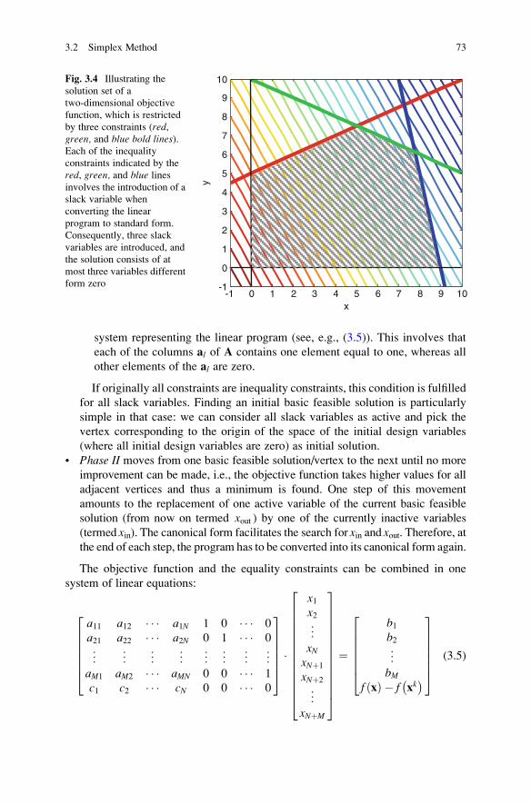
system representing the linear program (see, e.g., (3.5)). This involves that

each of the columns al of A contains one element equal to one, whereas all

other elements of the al are zero.

If originally all constraints are inequality constraints, this condition is fulfilled

for all slack variables. Finding an initial basic feasible solution is particularly

simple in that case: we can consider all slack variables as active and pick the

vertex corresponding to the origin of the space of the initial design variables

(where all initial design variables are zero) as initial solution.

• Phase II moves from one basic feasible solution/vertex to the next until no more

improvement can be made, i.e., the objective function takes higher values for all

adjacent vertices and thus a minimum is found. One step of this movement

amounts to the replacement of one active variable of the current basic feasible

solution (from now on termed xout ) by one of the currently inactive variables

(termed xin). The canonical form facilitates the search for xin and xout. Therefore, atthe end of each step, the program has to be converted into its canonical form again.

The objective function and the equality constraints can be combined in one

system of linear equations:

a11 a12 � � � a1N 1 0 � � � 0

a21 a22 � � � a2N 0 1 � � � 0

..

. ... ..

. ... ..

. ... ..

. ...

aM1 aM2 � � � aMN 0 0 � � � 1

c1 c2 � � � cN 0 0 � � � 0

2666664

3777775�

x1x2...

xNxNþ1

xNþ2

..

.

xNþM

26666666666664

37777777777775

¼

b1b2...

bMf xð Þ � f xk

� �

2666664

3777775

(3.5)

x

y

-1

0

1

2

3

4

5

6

7

8

9

10

-1 0 1 2 3 4 5 6 7 8 9 10


solution set of a

two-dimensional objective

function, which is restricted

by three constraints (red,green, and blue bold lines).Each of the inequality

constraints indicated by the

red, green, and blue linesinvolves the introduction of a

slack variable when

converting the linear

program to standard form.

Consequently, three slack

variables are introduced, and

the solution consists of at

most three variables different

form zero


where the first M rows represent the constraints and the last row represents the

objective function, with f xk� �

being its value at the current solution. (3.5) is often

referred to as the simplex tableau. If all M constraints are inequality constraints,

only the slack variables xNþ1 to xNþM are active in the initial basic feasible solution,

and, consequently, the lastM columns of the matrix contain only one element equal

to 1, all others are zero.

For the moment, let’s assume that the problem already is available in canonical

form. Then, phase II of the simplex algorithm proceeds as follows. Each iteration

has to asses which active variable xout is to be substituted and which inactive

variable xin will replace xout. Overall, each iteration comprises the following steps:

1. Specification of xin : This can be done by examining the coefficients of the last

row of (3.4). A negative coefficient ci < 0 indicates that the value of the

objective will decrease if the corresponding variable xi will become greater

than zero. Consequently, xin will be chosen such that the corresponding coeffi-

cient cin has the most negative value among all ci belonging to currently inactivevariables. If all such ci have positive values, no more improvement can be made

and the iteration stops.

2. Specification of xout: In order to find xout, the ratios bj aj;in�

are calculated for all

j 2 1; . . . ;M½ �. The index out is chosen such that bout aout;in�

has the smallest ratio

among all ratios whereaj;in is positive. In order to find the variablexout leaving thebasic feasible solution, we search for the active variable which has a coefficient

equal to 1 in row out.

3. Rearrangement of the simplex tableau such that it is canonical with respect to theupdated basic variables. This operation is called pivoting on the element aout;in.The goal is to modify the simplex tableau such that column ain contains only one

nonzero element at position out, which can be set to one, i.e., akþ1out;in ¼ 1 and all

other akþ1j;in ¼ 0. Therefore, the following two steps are performed:

1. Divide row out by aout;in. This ensures that akþ1out;in ¼ 1.

2. For all other rows j, multiply the updated rowout byaj;in and subtract the result

from row j. This ensures that akþ1j;in ¼ 0.

After the iteration has stopped, the ci of the non-basic (inactive) variables revealthe type of the solution:

• All ci are positive: the solution is unique.

• One or more ci’s are equal to zero: the solution is not unique.

• One or more ci’s are less than zero: the solution is unbounded.

An overview of the general proceeding can be seen in Fig. 3.5.

Let’s illustrate this proceeding with the help of a little example. Consider the

objective f xð Þ ¼ �3 � x1 � 1:5 � x2 þ 20 and the constraints � 0:5 � x1 þ x2 � 5,

5�x1 þ x2 � 45, and 0:5 � x1 þ x2 � 10 (see Fig. 3.4). For the initial basic feasible


solution x1 ¼ x2 ¼ 0 (black point in Fig. 3.6), the objective takes the value f 0ð Þ¼ 20. Hence, the simplex tableau can be written as

�0:5 1 1 0 0

5 1 0 1 0

0:5 1 0 0 1

�3 �1:5 0 0 0

2664

3775 �

x1x2x3x4x5

266664

377775¼

5

45

10

f xð Þ � 20

2664

3775 (3.6)

with x3 to x5 denoting the slack variables.

As all three constraints are inequality constraints, we have three slack

variables in total. (3.5) already is in canonical form, so we can directly proceed

with phase II of the simplex algorithm. The most negative coefficient of the last

row is �3 in the first column, so x1 will enter the solution. Consequently, the

first column of the matrix has to be considered for determining the variable

which has to leave the solution. There, we have two positive elements, with the

ratio of b2 a2;1�

being the smallest. Consequently, we have to pivot on a2;1. An

examination of row 2 reveals that x4 will leave the solution. Geometrically

speaking, this corresponds to a movement along the x-axis (indicated by the

black arrow in Fig. 3.6) to the vertex marked green in Fig. 3.6.

In order to rearrange the tableau to canonical form, we first divide row 2 by the

value 5 and then subtract the thus updated row �0.5 times from row 1 (thus add it

0.5 times), subtract it 0.5 times from row 3, and subtract it�3 times (add it 3 times)

from row 4. This yields the following updated simplex tableau:

Formulate program in

standard formS

Is program in canonical

form?

Convergence ?

no

no

yes

E

Solve modi-fied program with Phase II

Introduce artificial variables

yes

Specify ini-tial solution

Determinex in and xout

Re-establish canonical

form

Retrieve x∗

from the ci ´s

Fig. 3.5 Flowchart of the simplex method


0 1:1 1 0:1 0

1 0:2 0 0:2 0

0 0:9 0 �0:1 1

0 �0:9 0 0:6 0

2664

3775 �

x1x2x3x4x5

266664

377775¼

9:59

5:5f xð Þ þ 7

2664

3775 (3.7)

In the next iteration, we see that progress can still be made, as the second

coefficient of the last row is negative. Hence, x2 will enter the solution. As the

elements a1;2 , a2;2 , and a3;2 are all positive, the ratio of all of them has to

be calculated. Because b3 a3;2�

yields the smallest value, pivoting is done on a3;2,

and x5 leaves the solution (see Fig. 3.6: movement along the green arrow until the

red vertex is reached). According to step 3, the third row is to be divided by 0.9,

and the result is to be subtracted 1.1 times from row 1 and 0.2 times from row 2 and

added 0.9 times from the last row. As a result, the following updated simplex

tableau is obtained:

0 0 12

9� 11

9

1 0 02

9� 2

9

0 1 0 � 1

9

10

9

0 0 0 0:5 1

266666664

377777775

�

x1x2x3x4x5

266664

377775¼

25

9

70

9

55

9

f xð Þ þ 12:5

266666664

377777775

(3.8)

Now all coefficients in the last row belonging to non-basic variables are positive.

Consequently, the iteration stops and the obtained solution is unique. As x4 and x5are zero, the solution can be seen directly from equation (3.8). The first row reveals

that x3 ¼ 25 9= , from the second row we obtain x1 ¼ 70 9= , and the third row yields

x2 ¼ 55 9= .

x

y

−1 0 1 2 3 4 5 6 7 8 9 10−1

0

1

2

3

4

5

6

7

8

9


proceeding when optimizing

the linear program (3.6) with

the simplex method


Now let’s come back to phase I, which is needed if the standard form of the

linear program is not in canonical form at start. Consider replacing the second

constraint in the above example by � x1 þ x2 � �2 . Now b2 is negative, and

consequently, the program is not in its canonical form if the initial basic solution

contains the slack variables x3 to x5:

�0:5 1 1 0 0

�1 1 0 1 0

0:5 1 0 0 1

�3 �1:5 0 0 0

2664

3775 �

x1x2x3x4x5

266664

377775¼

5

�2

10

f xð Þ � 20

2664

3775 (3.9)

In order to make b2 positive, row 2 can be multiplied by �1, but, in turn, this

makes the coefficient of x4 negative. This means that x4 is not an active variable anylonger. A way out of this dilemma is to introduce another variable x6 (which is

appended to row 2, as row 2 was multiplied by �1) as well as another function x6¼ r . The introduction of x6 ¼ r means that we add another row to the simplex

tableau and treat the former last row belonging to the “real” objective as a constraint

equation. Now we have

�0:5 1 1 0 0 0

1 �1 0 �1 0 1

0:5 1 0 0 1 0

�3 �1:5 0 0 0 0

0 0 0 0 0 1

266664

377775�

x1x2x3x4x5x6

26666664

37777775¼

5

2

10

f xð Þ � 20

r

266664

377775

(3.10)

This tableau can be converted into canonical form by ensuring that only one

coefficient of the last column of the matrix is nonzero. This can be done if row 2 is

subtracted from row 6 yielding

�0:5 1 1 0 0 0

1 �1 0 �1 0 1

0:5 1 0 0 1 0

�3 �1:5 0 0 0 0

�1 1 0 1 0 0

266664

377775�

x1x2x3x4x5x6

26666664

37777775¼

5

2

10

f xð Þ � 20

r � 2

266664

377775

(3.11)

which now is in canonical form with the basic variables x3,x5, and x6. However, as x6doesn’t exist in the original problem, it has to be eliminated again. This can be done

by solving (3.11), i.e., finding a basic feasible solution which minimizes r. To this


end, the proceeding of phase II can be applied. If we end up with a solution which

sets r to zero (x6 ¼ r ¼ 0), we can eliminate x6 again (drop the last column as well as

the last row) and solve the remaining simplex tableau with phase II. However, if

the solution of phase I does lead to a solution where r 6¼ 0, a solution without the

artificial variable x6 cannot be found. This means that no solution exists for the

original linear program in that case.

Overall, phase I consists of the following steps:

1. Multiplication of all rows j which have a negative bj by �1, if necessary.

2. Introduction of as many artificial variables as necessary (introduce new variables

until there are M variables affecting only one constraint, i.e., “their” column

features only one nonzero value which is equal to 1).

3. Creation of a new objective function r, which is equal to the sum of all newly

introduced variables.

4. Converting the extended problem into canonical form by subtracting all rows

where new variables were introduced from the last row (such that the last row

contains zeros in all columns where the variables are part of the initial basic

feasible solution).

5. Solution of the just obtained linear program by applying phase II.

6. Elimination of the just introduced artificial variables in the case of r ¼ 0. If r 6¼ 0,

no solution exists.

Pseudocode

function solveLinearProgramSimplex (in objective functionf xð Þ, in constraints specified by A and b, out solution x�)

// conversion of linear program to standard formintroduce a slack variable for each inequality constraint inorder to convert it into an equality constraintsplit each non-restricted design variable into the differ-ence of two design variables restricted to non-negativevaluescreate the simplex tableau according to (3.5)

// conversion of simplex tableau into canonical form, ifnecessary (phase I)if linear program is not canonical then

for each row j where bj < 0

// not in accordance with canonical formmultiply row j by -1

nextadd new artificial design variables until M designvariables affect only one constraint (one element ofcolumn equals one, the others are zero)create a new objective r which equals the sum of all artifi-cial design variables


convert the thus obtained tableau into canonical form by rowsubtraction

// solve the modified linear program by executing phase IIcall solveSimplexPhaseII(f xð Þ, simplex tabl., out x�PI)if r ¼¼ 0 then

eliminate all artificial design variables againelseexit // no solution exists

end ifend if

// solve the linear program (phase II of the simplex method)call solveSimplexPhaseII(f xð Þ, simplex tableau, out x�)check the ci‘s in order to determine the kind of the solution

function solveSimplexPhaseII (in objective function f xð Þ, insimplex tableau specified by A and b, out solution x�)

specify initial basic feasible solution (contains onlyslack variables)

// iterative search loop (moves from vertex to vertex)repeat

// replace design variable xout by xinfind cin which has the most negative value (yields xin)

find the smallest ratio bj aj;in�

for all j 2 1::M½ � where aj;in > 0

(yields xout)// pivot on aout;in: re-establish canonical formdivide row out by aout;infor all other rows j

multiply the updated row out by aj;insubtract the result from row j

nextuntil convergence (all ci‘s are >¼0)retrieve solution x� form the ci ‘s of the current simplextableau

Over the years, many other solvers for linear programs have been developed.

One important class of solvers are the so-called interior point methods (sometimes

also called barrier methods), where the interior of the solution space is explored

(see, e.g., [4–6] or [7]). It can be proven that these methods are able to find the

optimum in polynomial time. On average, performance of interior point methods is

comparable to the simplex method. For practical examples, however, it depends on

the specific nature of the problem whether the simplex method or interior point

methods perform better.

If additionally the values of the design variables are required to be integers, the

resulting program is called an integer program. In contrast to linear programs, the


solution of these programs is NP-hard. For special subclasses, however, there exist

efficient solutions (see, e.g., [8]).

3.3 Example: Stereo Matching

Bhusnurmath et al. showed that stereo matching can be formulated as a linear

program [2]. In stereo matching, a scene is captured by a pair of cameras with

known geometric configuration, i.e., the distance between the two cameras as well

as the orientations of both cameras are known. Because the two cameras take a

different viewpoint, objects which are captured by both cameras appear with a shift

between them when we compare the two camera images.

This shift, which is also called disparity, is a function of the z-distance between

the object and the camera system (the so-called depth of the scene). The closer the

object, the larger is the disparity. Many computer vision tasks require an estimation

of the scene depth. If the cameras are calibrated, it is possible to infer the depth from

the disparity values. Hence, the problem of stereo matching amounts to estimating

the disparity di for each pixel pi. This process can also be thought of labeling each piwith the label di.

As already stated above, the z-distance between the object which is depicted at

pixel pi and the camera system can be directly derived from di if the camera

parameters and geometric relation between the two cameras are known. As a result,

a so-called height map can be calculated, which depicts the z-distance to the camera

system for each pixel of the image. Height maps can be used, e.g., in obstacle

avoidance applications.

The geometric configuration of the two cameras conditions that all disparities

appear in the same direction, i.e., the vectors between a pixel pi in the first image

and its “counterpart” in the second image point to the same direction for all pixels.

Therefore, we can search along a scan line with known direction when we want to

calculate a disparity d pið Þ for a given pixel pi, which will be denoted di for brevity inthe following. Usually it can be assumed that the scan line is a horizontal line

(which can be assured through the application of a preprocessing step known as

rectification). Consequently, if we examine all pixels with the same y-coordinate inboth images, we can determine the disparities for all pixels of this row. Addition-

ally, a proper choice of the reference camera ensures that all disparities are positive.

Now the question remains how to determine the disparities di . In [2], a joint

calculation of all disparities of a scan line in one optimization step is suggested.

To this end, an energyE dð Þ can be calculated for each scan line, which is a functionof the vector d accumulating all disparities di along this line. E dð Þ indicates howwell the di explains the content of the two images. If d is a good explanation, E dð Þshould be low. E dð Þ consists of two parts:

• A data-driven term Edata dið Þ, which measures how well the observed image data

at positionpi in the first image conforms to the observed image data in the second


image, shifted by di pixels, i.e., at position pi þ di. A common approach in stereo

for measuring how well the image data fits is to calculate some function (match

score) based on the cumulated intensity differences between

– all pixels located within an image patch around pixelpi (whose center positionin the first image is xi; yið Þ) and

– the pixels of the corresponding image patch centered at position xi þ di; yið Þ inthe second image.

• A so-called smoothness term Esmooth dið Þ takes into account that disparities tend

to be “smooth”. For example, it is quite common that the image shows multiple

planar objects with a surface normal parallel to the camera axis. As a conse-

quence, the disparities should be constant in areas covered by these objects and

develop steps at the object borders. Noise or artifacts, however, tend to introduce

variations between the disparities of adjacent pixels everywhere in the image

plane. In order to reduce the influence of noise, the total sum of the disparity

gradients (i.e., the difference of disparities between adjacent pixels) should be

small. Consequently, one part of Esmooth dið Þ , which we term Egrad di; diþ1ð Þ ,measures the sum of disparity gradient magnitudes between adjacent pixels piand piþ1. A second component, Elap di; diþ1; di�1ð Þ, takes the second derivatives

into account: if planar objects show out-of-plane rotation, i.e., their surface

normal is not parallel to the camera axis, the disparity map has gradients, but

no curvature. Therefore, the total curvature should be minimal.

Overall, the energy EðdÞ of a scan line can be modeled as follows1:

E dð Þ ¼XW

i¼1

Edata dið Þ þXW�1

i¼1

Egrad di; diþ1ð Þ þXW�1

i¼2

Elap di; diþ1; di�1ð Þ (3.12)

where W denotes the image width. The data-driven energy can be modeled by

intensity differences between corresponding image patches. The gradient-based

energy term should be high when the difference of the disparities of adjacent pixels

is high:

Egrad di; diþ1ð Þ ¼ 0 if di � diþ1j j � εwg;i � di � diþ1j j � εð Þ otherwise

�(3.13)

Through the introduction of ε, small disparity changes are not punished. wg;i is a

weighting parameter (corresponding to pixel pi ) and allows to adjust the relative

importance of a pixel. Consider the disparities at the edge between two objects, for

example: usually, the z-distance of the two objects differs, and consequently, the

1 For convenience, only the one-dimensional solution, where all disparities along one scan line are

estimated simultaneously, is presented here. However, the extension to the 2D case is possible and

rather straightforward.

3.3 Example: Stereo Matching 81

disparity shows a discontinuity at the edge between the objects. Therefore, the

weighting factors of these “edge pixels” obtain a low value in order to allow for

disparity discontinuities at these positions.

The second-order Laplacian term should punish high curvatures of the disparity

as many objects are assumed to be at least nearly planar. It can be set to the discrete

approximation of the Laplacian (once again with a weighting term wl;i):

Elap di; diþ1; di�1ð Þ ¼ wl;i � �di�1 þ 2di � diþ1j j (3.14)

In stereo matching, the goal is to find for each scan line the disparitiesd� such thatE dð Þ gets minimal for the line currently under consideration: d� ¼ argminE dð Þ .In order to solve this task, the authors of [2] suggest to convert the problem into a

linear program, which can then be solved by an appropriate linear program solver.

This problem formulation has the advantage that the continuous nature of linear

programs avoids quantization at intermediate steps (opposed to discrete methods,

which are widely used for stereo matching).

Concerning the smoothness terms, the objectives Egrad and Elap are not linear in

the design variablesdbecause of the absolute values. In order to convert these terms

into linear relations, additional variables are introduced and, additionally,

constraints are built for these additional variables.

Let’s consider Egrad, for example: For each pixel, Egrad is set to a proxy variable

yg;i , weighted by wg;i : Egrad di; diþ1ð Þ ¼ wg;i � yg;i . If di � diþ1j j > ε and therefore

yg;i > 0, we have to consider two cases: Ifdi > diþ1, yg;i is set to yg;i ¼ di � diþ1 � ε.Respectively, we have to set yg;i ¼ diþ1 � di � ε in the case of di < diþ1 . This

ambiguity can be resolved by replacing the equality by three inequalities which

have to be fulfilled simultaneously:

yg;i � di � diþ1 � εyg;i � diþ1 � di � ε0 � yg;i � gmax

(3.15)

Considering the first two inequalities, we can see that one of them is more

restrictive than the other, i.e., if the more restrictive is fulfilled, the other holds,

too. Whether the first or second is more restrictive depends on the sign of di � diþ1.

With the help of this little “trick,” we managed to achieve linearization. The third

inequality constraint ensures positivity for yg;i and that it is upper-bounded by gmax.

Similar considerations can be made for Elap and lead to

yl;i � �di�1 þ 2di � diþ1

yl;i � di�1 � 2di þ diþ1

0 � yl;i � lmax

(3.16)


The upper bounds gmax and lmax respect the fact that disparity values are bounded

in practice.

Please note that in general the calculation of the data term of the energy by

summing up intensity differences as described above is not linear nor convex.

However, this would be desirable, because if the objective is known to be convex,

it is assured that a found local minimum is also the global minimum. A typical

example of the data-driven energyEdata dið Þat one pixel is shown in the blue curve ofFig. 3.7, where the pixel-wise energy is calculated dependent on the assumed

disparity value. Clearly, this function is not linear nor convex. Therefore, the

function is approximated by piecewise linear functions aj;idi þ bj;i, which act as a

lower bound of the energy Edata dið Þ (see red curve in Fig. 3.7).

In order to formulate the stereo problem as a linear program, another auxiliary

variable ym;i is introduced for each pixel. ym;i directly measures the data-driven

energy at this pixel. The line segments of the piecewise linear convex approxima-

tion serve as constraints, which ensure that ym;i is always located above all line

segments, e.g., above all red line segments shown in Fig. 3.7. Altogether,

concerning Edata dið Þ, we haveEdata dið Þ ¼ wm;i � ym;iym;i � aj;idi þ bj;i; j 2 1; 2; . . . ; J½ �0 � ym;i � ymax

(3.17)

The final formulation of the energy is given by

5

6

7

8

9

10

11

12

13

14

15

16

5 10 15 20 25 30 35 40 45 50 55 60

E_Data

Disparity

Fig. 3.7 Illustrating the data-driven energy for different disparities (blue) and its convex lower-

bound approximation

3.3 Example: Stereo Matching 83

E dð Þ ¼XW

i¼1

wm;i � ym;i þXW�1

i¼1

wg;i � yg;i þXW�1

i¼2

wl;i � yl;i (3.18)

The weights wm;i should reflect the degree of confidence in the match score

(obtained through intensity comparisons) and should be low in occluded areas.

Gradient and Laplacian weights wg;i and wl;i are based on the intensity or color

difference between the pixels under consideration and therefore should be low if the

pixels belong to different objects (which are likely to have differing colors or

intensities). Therefore, they allow for clear disparity discontinuities between

objects without penalizing.

(3.17) can be written as the linear functionwT � x, wherex is a vector concatenatingall design variables: x ¼ d ym yg yl

� �Tand w is a vector containing the

corresponding weights: w ¼ 0 wm wg wl½ �T . To sum it up, (3.15, 3.16, 3.17,

and 3.18) build a linear program, as all equations and inequality constraints are linear

in the design variables. Consequently, this program can be solved by an appropriate

optimization scheme for linear programs like the simplex method.

Details of the composition of the constraints as well as the solver employed

(Bhusnurmath et al. chose an interior point method as a solver) can be found in [1,

2] and are beyond our scope here.

To sum it up, the algorithm estimating the disparities for one row of the images

consists of the following steps:

1. Calculation of Edata dið Þ for all legal disparities and all pixels

2. Approximation of Edata dið Þ with piecewise linear functions for each pixel

3. Estimation of the weights w ¼ 0 wm wg wl½ �T4. Formulation of the linear program with the help of the introduction of the

auxiliary variables ym, yg, and yl5. Solution of the linear program with an interior point barrier method

Please observe that the dimensionality of the linear equation system is very

large, as the number of design variables is four times the number of pixels.

Moreover, the number of constraints is quite high as well. For example, a closer

look at (3.16) reveals that for each pixel there existJ constraints, whereJ denotes thenumber of line segments used for convex approximation. This leads to rather long

execution times, albeit because of linearity a fast optimization scheme can be

employed. With a MATLAB-based implementation, the authors of [2] reported

running times in the order of minutes.

Results for some images of the Middleburry data set (which is often used to

compare the performance of stereo matching algorithms) can be found in the

original article [2]. As can be seen there, the height map calculated by the algorithm

is very close to the ground truth. Please observe that the algorithm intends to “fill

gaps” at pixels where there is no reliable data available due to occlusion.


References

1. Bhusnurmath A (2011) Applying convex optimization techniques to energy minimization

problems in computer vision. PhD thesis, Proquest Umi Dissertation Publishing, Philadelphia.

ISBN 978–1243494221

2. Bhusnurmath A, Taylor CJ (2008 ) Solving stereo matching problems using interior point

methods. In: Fourth international symposium on 3D data processing, visualization and trans-

mission, pp 321–329

3. Dantzig GB (1951) Maximization of a linear function of variables subject to linear inequalities.

In: Activity analysis of production and allocation. Wiley, New York, pp 339–347

4. Dantzig GB, Thapa MN (1997) Linear programming: 1: introduction. Springer, New York.

ISBN 978-0387948331

5. Fang S-C, Puthenpura S (1993) Linear optimization and extensions: theory and algorithms.

Prentice Hall, Englewood Cliffs. ISBN 978-0139152658

6. Gondzio J, Terlaky T (1994) A computational view of interior point methods for linear

programming. In: Advances in linear and integer programming. Oxford University Press,

Oxford

7. Karmarkar N (1984) A new polynomial-time algorithm for linear programming. In: Proceedings

of the sixteenth annual ACM symposium on theory of computing, New York, pp 302–311

8. Nemhauser G, Wolsey A (1999) Integer and combinatorial optimization. Wiley, New York.

ISBN 978-0471359432

References 85

Chapter 4

Variational Methods

Abstract The main goal of many computer vision tasks can in summary be

described by finding a function which is optimal according to some criteria.

Examples of such functions are the two-dimensional intensity/color function of

the image itself in image restoration or deblurring, two-dimensional vector fields

like optical flow, or the course of a curve separating the image into multiple areas

(which are all presented as examples in this chapter). This is the domain of

variational optimization, which aims at estimating those functional relationships.

The functional quantifying the quality of a particular solution typically consists of

two terms: one for measuring the fidelity of the solution to the observed data and a

second term for incorporating prior assumptions about the expected solution, e.g.,

smoothness constraints. There exist several ways of finding the solution, such as

closed-form solutions via the so-called Euler-Lagrange equation, or iterative

gradient-based schemes. Despite of the iterative and therefore inherently slow

nature of the last-mentioned approach, quite simple iterative update rules can be

found for some applications, which allow for a very fast implementation on

massively parallel hardware like GPUs. Therefore, variational methods currently

are an active area of research in computer vision.

4.1 Introduction

4.1.1 Functionals and Their Minimization

Variational optimization deals with the problem of directly finding optimal

functions themselves. This means that the solution space is composed of functions

as elements. Compared to that, the methods presented up to now reduce the degrees

of freedom when seeking the solution by fixing the structure of the function in

advance. In that case, optimization is about estimating the parameters of the

specified function type. For example, the shading correction algorithm we encoun-

tered already in Chap. 2 as an example of regression a priori specifies that the



87

http://dx.doi.org/10.1007/978-1-4471-5283-5_2

shading has to be modeled by a two-dimensional polynomial up to a certain order.

During optimization, just the values of the coefficients of the polynomial terms are

calculated, whereas the design of the objective function remains unchanged. In

contrast to that, a variational approach would make no a priori assumptions about

the course of the shading function – any course would be allowed for the solution.

Let’s further examine this concept with the help of another short example: given

two points p and q in the two-dimensional xy-plane, we want to find the curve

connecting these two points with minimal arc length. The course of the curve can be

expressed by a functional relationship, and therefore, the task is to find the function

that minimizes the arc length. Intuitively, we all know that the shortest connection

between p and q is given by a straight line segment. But how can we find this

solution mathematically? This can be done as follows (see also [6]):

Positions on the curve can be expressed as x; yðxÞð Þ. Hence, our aim is to find a

functional relationship y�ðxÞ which minimizes the arc length. Let the position of pand q be expressed by p ¼ a; yðaÞð Þ and q ¼ b; yðbÞð Þ. The arc length ly can be

derived by integrating over the length of infinitesimal straight line segments and is

given by

ly ¼Z b

a

ffiffiffiffiffiffiffiffiffiffiffiffiffiffiffiffiffiffiffiffi1þ y0ðxÞ2

qdx (4.1)

where y0ðxÞ denotes the first derivative of y with respect to x : y0ðxÞ ¼ dy dx= .

Consequently, the desired y�ðxÞ can be found by minimizing (4.1).

A more general formulation of (4.1) is

F yðxÞ½ � ¼Z b

a

f x; yðxÞ; y0ðxÞð Þdx (4.2)

Functions like F are called functionals, which have the characteristic that they

map a function to a scalar value. The task of variational optimization is then to find

the argument y�ðxÞ (which is a function) of F yielding the smallest value of F, i.e.,y�ðxÞ is the minimizer F . Please note that the goal of finding a function is just

conceptually. In practice, usually numerical implementations try to find a

discretized version of y�ðxÞ , where the quantities y�i xið Þ at sampled positions xiare to be found. Hence, in practice usually we seek a finite set of function values.

The minimization of (4.2) can be performed with a paradigm called calculus ofvariations (see [6] for a good introduction). We can formulate a necessary condition

for y�ðxÞ being a local minimum of the functional F, which is known as the Euler-Lagrange equation. The Euler-Lagrange equation relates to the fact that for minima

of “ordinary” functions, the first derivative of the function to be minimized must be

equal to zero. The Euler-Lagrange equation transfers this to functionals with

functions as arguments. It is a partial differential equation and is given by

@f

@y� d

dx

@f

@y0

� �¼ 0 (4.3)

88 4 Variational Methods

The name “calculus of variations” comes from the proceeding when solving

the Euler-Lagrange equation, where a set of functions, whose elements are all

variations of yðxÞ, is considered.The calculus of variations tries to solve (4.3) for a given problem (which is

usually done iteratively) and then assumes that this solution is the desired solution

y�ðxÞ. Observe, however, that (4.3) is only a necessary condition, and, moreover, we

don’t know whether F has a minimum at all. Consequently, we have no guarantee

that we actually find the desired minimum when applying the calculus of variations.

A quite common case is that f does not directly depend on x, i.e., we can write

f yðxÞ; y0ðxÞð Þ. Then (4.3) simplifies to

f � y0 � @f@y0¼ C (4.4)

where C is a constant. This is known as the Beltrami identity.The general form of F is suited for many vision applications. Consider the

examples of image restoration (e.g., denoising or deconvolution) being described in

detail in the next section. In restoration applications, we want to infer the original

version of an image R x; yð Þ (i.e., we seek a function) but only have access to the

observed data I x; yð Þ, usually corrupted by noise and/or blur. This kind of problem is

said to be an inverse problem, where, based on some observations, we want to

“infer” the unobservable but uncorrupted original signal.

As R x; yð Þ should be close to I x; yð Þ, f should reflect a measure of difference

between the two signals. Additionally, we can also assume that R x; yð Þ varies onlysmoothly in many regions, e.g., because many objects are of uniform or slowly

varying brightness/color. This is known as the so-called smoothness assumption.

Consequently, f is also influenced by the derivative of R x; yð Þ.Hence, f can be interpreted as measuring the suitability of R x; yð Þ being a

plausible explanation of I x; yð Þ at a particular position x; y½ �. However, we want tofind a function which best explains the observed data in the entire image. Accord-

ingly, we integrate f over the image area, which leads us to formulating the problem

such that a functional of the form of F is to be minimized.

The general proceeding of utilizing the calculus of variations in variational

optimization of computer vision problems can be summarized as follows:

1. Formulate f such that it reflects the suitability for yðxÞ explaining some observed

data x:2. Add a smoothness constraint to f . Usually, this constraint is independent of x but

relates to some derivative information of yðxÞ.3. Build the variational integral F being based on f .4. Find the solution by calculating the minimizing argument y�ðxÞ of F.

Step 4 usually requires some discretization step in practice. There does not exist

a standard proceeding for this step. One possibility is to set up the Euler-Lagrange

equation explicitly first and then calculate the (discretized) minimizer of a

discretized version of it (e.g., for active contours, see Sect. 4.5). Another option

4.1 Introduction 89

is to perform discretization at an early stage in the domain of f . This proceedingseems natural in image restoration tasks (see Sects. 4.2 and 4.3), where I x; yð Þalready is available in discretized form along the pixel grid. As a consequence, F is

present in a discretized version, too. Its minimizing argument can therefore be

expressed by a finite set of values at the sample positions.

Before we take a closer look at some variational methods in detail, let’s make

some comments on the quality of solutions obtained with variational methods in

practice. Please note that many variational schemes are local methods (e.g., the

Euler-Lagrange equation acts only locally) and therefore lead to solutions which are

the best among just a local neighborhood (local optima). Consequently, we cannot

be sure that its solution indeed is the desired global optimum.

However, the functionals utilized in practice in many computer vision

applications are so-called convex functions. Geometrically speaking, this means

that if we connect any two points x1; f x1ð Þ½ � and x2; f x2ð Þ½ � by a straight line, the linesegment between these two points is always “above” the course of the function f(see Fig. 4.1). If this condition holds, f is convex. Mathematically speaking, f is

convex if

f θ � x1 þ 1� θð Þ � x2ð Þ � θ � f x1ð Þ þ 1� θð Þ � f x2ð Þ (4.5)

Convex functions, in turn, have the nice property, that they have only one

minimum, which therefore is ensured to be the global one. Consequently, if we

know that the functional of our problem at hand is convex, we can be sure that a

local optimum found has to be the global one, too.

In situations where the functional does not satisfy (4.5), there often exists the

following resort: sometimes we can “relax” the functional to a different functional,

0

10

20

30

40

50

60

−5

−4.5 −4

−3.5 −3

−2.5 −2

−1.5 −1

−0.5 0

0.5 1

1.5 2

2.5 3

3.5 4

4.5 5

f(x)

x

Fig. 4.1 Exemplifying a convex function (black curve). Each straight line segment connecting

two points on the function lies “above” the function. The red and green dashed lines are two

examples of this


which serves as a lower bound of the original functional and is convex at the same

time. Thus, the global optimum of that relaxed functional can be found. As this

relaxed functional is not equal to our original functional, the thus obtained solution

is only an approximation of the true optimum. However, it can sometimes be shown

that there is an upper bound for the difference between the exact solution and the

approximation, e.g., a small constant factor. Thus, the strategy of approximating the

functional by a convex lower bound and taking the global optimum of the lower

bound functional yields quite good performance in practice.

4.1.2 Energy Functionals and Their Utilizationin Computer Vision

Functionals in the form of (4.2) are appropriate to represent many computer vision

applications. They often act as an energy E being able to judge the suitability of a

particular solution y. The energy is high if y doesn’t represent an adequate solution.This can be explained best by considering a typical application, namely, resto-

ration. Restoration techniques are applied to reconstruct or infer “cleaned” data

without artifacts, given some measured data. In our case we deal with restoration of

images, where, given some sensed image data I x; yð Þ , the task is to infer the

reconstructed version R x; yð Þ of the original unobserved image R x; yð Þ. Noise and

sometimes also other effects like blur, which are inevitably present to some

extent in I, should be removed in R. In this application, the relationship between

R and I can be modeled by

I x; yð Þ ¼ K � R x; yð Þ þ n ¼ð ð

K a; bð ÞR a� x; b� yð Þda dbþ n (4.6)

where n is a noise term, * is the convolution operator, and K denotes a convolution

kernel which typically models some kind of blur, e.g., motion or camera defocus.

The problem of estimating R given I is called ill-posed, because there exist many

solutions for a particular I and we are faced with the problem which one to choose.

This comes from the fact that there are more unknowns than observations: Let Ndenote the number of pixels. Then, considering I, we haveN observations, but more

than N unknowns, because we have to estimate N pixel values of R and, in addition

to that, the blur kernel K.The removal of the ill-posedness is tackled by designing an energy functional E,

which measures the “goodness” of R being a proper reconstruction of R. The higher

the value (“energy”) of E, the less suited is R for a reconstruction of R. Hence,through the usage of E, several possible solutions can be rated with respect to their

suitability for being a good reconstruction.

Additionally, new information can easily be introduced inEvia additional terms.

This is necessary in order to overcome the under-determination. This technique is

4.1 Introduction 91

known as regularization, which enables us to solve the originally ill-posed problem.

In most cases we can make a priori assumptions about the functions to be found

(e.g., often the function to be searched is likely to vary only smoothly) and thereby

introduce additional information. As a summary, through the usage of E , the

original ill-posed problem should be turned into an optimization problem which

is well posed.

Now let’s come back to the restoration example. To make things simple, the

effect of the kernelK is neglected for now. As a consequence, the restoration task is

reduced to remove the image noise, which is also known as denoising. Then, a

reasonable optimization criterion is that R should be close to I , which can be

expressed by the data-driven energy term Ed:

Ed ¼ð ð

R x; yð Þ � I x; yð Þ� �2dx dy (4.7)

Obviously, this criterion is not sufficient, because it is solved by the trivial

solution R ¼ I . Therefore, we have to make additional assumptions in order to

obtain a proper solution. This comes in the form of a priori knowledge: most images

are composed of a certain number of regions with relatively small intensity (or

color) changes inside each region, e.g., because some rather uniform object (like a

car where most of the region depicts the (uniform) finish of the car) or background

(like blue sky) is depicted there. Therefore, R should be smooth, which can be

expressed by a smoothness-based energy term Es , which is based on the first

derivative of R:

Es ¼ð ðrR x; yð Þ�� 2

2dx dy (4.8)

where rR x; yð Þ denotes the gradient vector of R: rR ¼ @R @x= ; @R @y=� T

and the

operator �k k2 refers to the Euclidean vector norm (or L2 norm), i.e., rR x; yð Þ�� 22

¼ @R @x=� �2 þ @R @y=

� �2. In other words, the accumulated squares of gradient

strengths should be as small as possible.

Please note that the sensed data is in general corrupted by noise, which

introduces additional gradients and reduces overall smoothness. Therefore, Es

ensures that noise is suppressed during reconstruction, which is a desirable effect.

Es, which incorporates prior information (i.e., Es is independent of the observed

data), is also called a regularization term, because it should regulate the solution

such that a “simple” explanation of the observed data is found. “Simple” solutions

should be favored among the set of possible solutions, according to a principle

called “Occam’s razor”.


The incorporation of different terms in E is quite common for variational

optimization. Typically, E is composed of two or three components:

• The data-driven term Ed measures how well a particular solution is in accord

with the sensed data. The lower the Ed, the better is the fidelity of the solution to

the data.

• With the help of the so-called internal energy Eint , a priori knowledge can be

incorporated into the solution. Roughly speaking, Eint is a measure how likely a

solution occurs. In the denoising example, we know that R will probably be

smooth and thereforeEs represents the total sum of the magnitudes of the squared

gradients.

• Sometimes, a third term Eext, which is called external energy, is introduced in E.Eext captures how well a particular solution represents external specifications.

For example, Eext can be used to represent the accordance to user input.

In our case, the optimization problem can now be formulated by

R� ¼ minRðEÞ with E ¼ Ed R; I

� �þ α � Es R� �

(4.9)

where the Lagrange multiplier α controls the effect of smoothing. This design of

energy functionals consisting of two parts (data fidelity term and constraint based

on prior knowledge) is able of representing a large variety of problems and

therefore of widespread use in computer vision. Examples will follow in the next

sections.

4.2 Tikhonov Regularization

Tikhonov [26] (see also [1]) provided the mathematical framework for optimization

of functionals as defined in (4.7, 4.8, and 4.9) and, in particular, showed that the

solution R� of the now well-posed optimization problem (4.9) is a reasonable

approximation of the originally ill-posed problem. We speak of Tikhonov regulari-zation if the regularization term involves the usage of square terms (here the

integral of the squares of gradient magnitude in (4.8)). The utilization of squared

L2 terms also involves differentiability of the energy, and, moreover, the existence

of a closed-form solution (which means that a fast calculation of the solution is

possible), as we will see shortly.

For a numerical solution, the denoising problem has to be discretized. The

data-driven energy Ed turns into

Ed ¼XW�1

x¼0

XH�1

y¼0w x; yð Þ R x; yð Þ � I x; yð Þ� 2

(4.10)

4.2 Tikhonov Regularization 93

where W and H denote the width and height of the image, respectively. Moreover,

due to readability, continuous and discrete versions of some variables are named

identically. The contribution of each pixel can be weighted by a factor w x; yð Þ .The introduction of w x; yð Þ admits to deal with areas where no measurements are

available or assumed to be uncertain. If measurements are not available, w x; yð Þ isset to zero. At positions where measurements are present, w x; yð Þ can be used

to control how strongly the solution is forced to be equal or near sensed data.

A reasonable choice of w x; yð Þ is to set it to the inverse variance of the measured

data in a neighborhood around x; yð Þ: If there is little variance, data measurements

are supposed to be reliable, and, therefore, the solution should be similar to

measured data. Please note that the w x; yð Þ are known factors during optimization,

as they can be calculated solely based on I x; yð Þ in advance.

The discrete version of the smoothness termEs can be obtained via finite element

analysis. Terzopoulos showed in [25] that in our case Es has an especially simple

form:

Es ¼XW�1

x¼0

XH�1

y¼0sx x; yð Þ R xþ 1; yð Þ � R x; yð Þ þ @I @x= x; yð Þ� 2þ

þXW�1

x¼0

XH�1

y¼0sy x; yð Þ R x; yþ 1ð Þ � R x; yð Þ þ @I @y= x; yð Þ� 2 ð4:11Þ

where sx x; yð Þ and sy x; yð Þ are optional smoothness weights and control the degree of

smoothing. They can be set, for example, inversely proportional to the gradient

magnitude rI x; yð Þj j. As a result, in locations with strong gradients, which indicate

the presence of an edge in the image, the smoothness constraint is rather loose.

Again, sx x; yð Þ and sy x; yð Þ depend only on I x; yð Þ and therefore can be calculated

in advance. Consequently, they are not part of the optimization.

In its discrete form, it is possible to rearrange the energy functionalE ¼ Ed R; I� �

þα � Es R� �

(which is composed of (4.10) and (4.11)) as a quadratic form:

E ¼ rTAr� 2rTbþ c (4.12)

The vector r is obtained by a row-wise stacking of the 2D data R x; yð Þ :r ¼ R 0; 0ð Þ; R 1; 0ð Þ; . . . ; R w� 1; 0ð Þ; R 0; 1ð Þ; R 1; 1ð Þ; . . . ; R w� 1; 1ð Þ; . . . ; R

�

w� 1; h� 1ð Þ�T. The matrix A is composed of weighting factors originating from

those terms in (4.10) and (4.11) containing the square of some R. This rearrange-ment is important, because the quadratic form (4.12) enables us to derive a closed-

form solution by setting its first derivative to zero, as illustrated in Chap. 2.

In order to illustrate the calculation ofA, let’s first rewrite one term of the sum of

(4.11) (where no summarization is performed for mixed terms):


http://dx.doi.org/10.1007/978-1-4471-5283-5_2

sx x; yð ÞR xþ 1; yð Þ2 � R xþ 1; yð ÞR x; yð Þ þ R xþ 1; yð Þ@I @x= x; yð Þ�� R x; yð ÞR xþ 1; yð Þ þ R x; yð Þ2 � R x; yð Þ@I @x= x; yð Þþþ @I @x= x; yð ÞR xþ 1; yð Þ � @I @x= x; yð ÞR x; yð Þ þ @I @x= x; yð Þ2

26664

37775þ

þ sy x; yð ÞR x; yþ 1ð Þ2 � R x; yþ 1ð ÞR x; yð Þ þ R x; yþ 1ð Þ@I @y= x; yð Þ�� R x; yð ÞR x; yþ 1ð Þ þ R x; yð Þ2 � R x; yð Þ@I @y= x; yð Þþþ @I @y= x; yð ÞR x; yþ 1ð Þ � @I @y= x; yð ÞR x; yð Þ þ @I @y= x; yð Þ2

26664

37775

(4.13)

For illustrative purpose, let’s assume for the moment that r contains only three

elements and, accordingly, A is a 3�3 matrix. Then, rTAt can be written as

r0 r1 r2½ � �a00 a01 a02

a10 a11 a12

a20 a21 a22

264

375 �

t0

t1

t2

264

375 ¼

r0a00 þ r1a10 þ r2a20

r0a01 þ r1a11 þ r2a21

r0a02 þ r1a12 þ r2a22

264

375

T

�t0

t1

t2

264

375 ¼

r0a00 þ r1a10 þ r2a20ð Þ � t0 þ r0a01 þ r1a11 þ r2a21ð Þ � t1þr0a02 þ r1a12 þ r2a22ð Þ � t2

(4.14)

A closer look at (4.14) reveals that the row index of A selects which component

of r contributes to the sum, whereas the column index ofA selects which component

of tcontributes to the sum. For example, if r0 and t2 should make a joint contribution,

a02 has to be different from zero. With this knowledge, we can derive from (4.13)

which summand of (4.13) makes a contribution to which element ofA. For example,

in order to consider the term � α � sx x; yð Þ � R xþ 1; yð ÞR x; yð Þ , the element

ay�wþxþ1;y�wþx has to be incremented by � α � sx x; yð Þ . Now we can go through

(4.13) and identify all terms which contribute to some element of A (the ones which

contain products of two elements of R, either square products of the same element or a

product of two different elements) and, based on the indices of these elements, derive

the indices of the element ofA towhich theymake a contribution. Observe thatwe also

have one quadratic term of R in (4.10), which has to be considered, too. Altogether,

one term of the sums of (4.10) and (4.11) contributes to the elements ofA as follows:

ay�wþxþ1;y�wþxþ1þ ¼ α � sx x; yð Þay�wþxþ1;y�wþx� ¼ α � sx x; yð Þay�wþx;y�wþxþ1� ¼ α � sx x; yð Þay�wþx;y�wþxþ ¼ w x; yð Þ þ α � sx x; yð Þ þ α � sy x; yð Þ

a yþ1ð Þ�wþx; yþ1ð Þ�wþxþ ¼ α � sy x; yð Þa yþ1ð Þ�wþx;y�wþx� ¼ α � sy x; yð Þay�wþx; yþ1ð Þ�wþx� ¼ �α � sy x; yð Þ

(4.15)

4.2 Tikhonov Regularization 95

The complete matrixA can be built based on (4.15) if all x 2 0; . . . ;W � 2½ � andy 2 0; . . . ;H � 2½ � are considered.

Similarly, we can compute the increments of b by considering all terms of (4.10)

and (4.11) which contain one element of R:

by�wþxþ1þ ¼ 2α � sx x; yð Þ � @I @x= x; yð Þby�wþx� ¼ 2α � sx x; yð Þ � @I @x= x; yð Þþ

þ 2α � sy x; yð Þ � @I @y= x; yð Þ þ 2w x; yð Þ � I x; yð Þb yþ1ð Þ�wþxþ ¼ 2α � sy x; yð Þ � @I @y= x; yð Þ

(4.16)

Now that we know how to build the energy functional E in its quadratic form

(4.12), we can proceed with the question how to calculate the solution R� whichminimizesE. A necessary condition forR�minimizingE is that the first derivative is

zero at this point: @E @R

R�ð Þ ¼ 0. This relates to applying the Euler-Lagrange

equation for variational energy functionals. Considering E in its quadratic form,

setting its derivative to zero yields a closed-form solution, which has the convenient

property that it is linear in the unknowns and therefore simple to calculate. It can be

found when we solve the following linear system:

Ar� ¼ b (4.17)

Provided that A is non-singular, this linear system of equations could be solved

with a standard method like QR decomposition or directly with singular value

decomposition (SVD) of A (see, e.g., [7]). However, please consider that A is

extremely large (its dimensions are W � H �W � H, and, thus, the number of rows/

columns of A amounts to several hundreds of thousands or even millions), which

usually makes the usage of such general techniques prohibitive in terms of runtime

and memory demand.

In order to solve (4.17) efficiently, we have to exploit the special structure of A.Taking a closer look at (4.15) reveals that each pixel affects seven elements of Awhich are arranged in a symmetrical structure. It is easy to see that for pixel (0,0)

these elements are also symmetric with respect to the diagonal of A . As each

successive pixel affects elements which are shifted by one row as well as diago-

nally, the whole matrix A is symmetric and multi-banded. Each row has five

elements which are nonzero (except for the first and last rows of A ). As a

consequence, A is extremely sparse. This fact, in turn, can be exploited when

solving (4.17). There exist special techniques making use of this fact like multigrid

methods or conjugate gradient methods. A detailed description is beyond the scope

of this book. The interested reader is referred to [2].

As far as the capability of the method is concerned, we can conclude that the

regularization term efficiently removes noise (see Fig. 4.2, where the Tikhonov

solution for a denoising example of a butterfly image is depicted in the lower left).However, the L2 norm of the regularizer strongly penalizes large gradients, which

has the undesirable effect of oversmoothing step edges. A method avoiding this

kind of artifacts is presented in the next section.


4.3 Total Variation (TV)

4.3.1 The Rudin-Osher-Fatemi (ROF) Model

There exist implementations of regularization techniques being different from

Tikhonov’s approach. More specifically, they differ in the calculation of the regulari-

zation term Es. For example, if we take the integral of the absolute gradients instead

of the squared magnitudes, we talk about total variation regularization, which was

first used in an image processing context by Rudin et al. [22] for noise suppression.

When we use total variation as a regularizer, we make use of the observation that

noise introduces additional gradient strength, too. In contrast to Tikhonov regulari-

zation, however, total variation takes the absolute values of the gradient strength

as regularization term, which is rR x; yð Þ�� ¼ffiffiffiffiffiffiffiffiffiffiffiffiffiffiffiffiffiffiffiffiffiffiffiffiffiffiffiffiffiffiffiffiffiffiffiffiffiffiffiffiffiffiffiffiffiffiffiffi@RR @x=� �2 þ @R @y=

� �2q. Conse-

quently, the energy functional of Rudin et al. can be written as

Fig. 4.2 Illustrating the performance of total variation regularization. Upper left: original image.

Upper right: image with synthetically added noise. Lower left: denoising solution with Tikhonov

regularization. Lower right: denoising solution with total variation (From Pock [20], with kind

permission)

4.3 Total Variation (TV) 97

ETV ¼ 1

2λ�ð ð

R x; yð Þ � I x; yð Þ� �2dx dyþ

ð ðrR x; yð Þ�� dx dy (4.18)

According to first letters of the names of the authors of [22], Rudin, Osher, and

Fatemi, this energy functional is also known as the ROF model in literature.

The smoothness term differs fromTikhonov regularization, where the L2 norm of

the gradient strength is used. A disadvantage of the L2 norm is that it tends to

oversmooth the reconstructed image because it penalizes strong gradients too much.

However, sharp discontinuities producing strong gradients actually do occur in real

images, typically at the boundary between two objects or object and background. In

contrast to the L2 norm, the absolute gradient strength (or L1 norm of the gradient

strength) has the desirable property that it has no bias in favor of smooth edges. The

shift from L2 to L1 norm seems only a slight modification, but in practice it turns

out that the quality of the results can be improved considerably, because the bias to

oversmoothed reconstructions is removed efficiently.

Compare two situationswhere an intensity increase of 100 gray values occurswithin

just a few pixels (situation A) or is distributed along very many pixels (situation B).

Clearly, the square operation in Tikhonov regularization favors situation B, because

the gradient is significantly lower at each pixel here, and, therefore, the sum of the

squared gradients is lower compared to situationA. Total variation, however, does not

favor any of the two situations, because the absolute sum remains 100 gray values for

both situations, regardless of its distribution. As a consequence, step edges, which

occur quite often, are preserved during regularization.

An example of the impact of moving from Tikhonov regularization to total

variation-based denoising can be seen in Fig. 4.2. In the upper left part, we can see

an image of a butterfly with many structures at a fine level of detail. Synthetic noise

has been added to the upper right image. The two lower images are obtained by

applying denoising with Tikhonov regularization (left) as well as total variation

denoising (right). Both schemes are able to suppress the noise, but clearly the TV

norm yields a much better result, because the edges are preserved much better.

On the other side, albeitETV is convex and therefore a unique solution exists, the

regularization term of ETV is not differentiable when rR tends to zero because

of the L1 norm. This means that a closed-form solution is not possible here.

Consequently, the solution is more difficult to calculate compared to Tikhonov

regularization. In particular, the absence of a closed-form solution requires an

iterative scheme, which is computationally more complex. However, as we will

see later, the iteration can be implemented very efficiently on massively parallel

processing units such as GPUs, because it can be parallelized very well.

4.3.2 Numerical Solution of the ROF Model

A technique for solving (4.18) numerically, which leads to a quite simple update

procedure, was suggested by Chambolle [3]. The derivation is rather complicated;


therefore, only an outline will be given here. The interested reader is referred to

[3, 4, 20] for details.

In order to obtain a solution, Chambolle transforms the original problem into a

so-called primal-dual formulation. The primal-dual formulation of the problem

involves the usage of a 2-dimensional vector field p x; yð Þ ¼ p1 x; yð Þ; p2 x; yð Þ½ � .The vector field p is introduced as an auxiliary variable (also termed dual variable)

and helps to convert the regularization term into a differentiable expression. With

the help of p, the absolute value vj j of a 2-dimensional vector v can be rewritten as

vj j ¼ suppj j�1

v; ph i (4.19)

where �h i denotes the dot product and can be written as v; ph i ¼ vj j � pj j � cos θ, i.e.,the product of the lengths of the two vectorsvandpwith the angleθ in between thesetwo vectors. If pj j ¼ 1 and, furthermore, v and p point in the same direction (i.e.,

θ ¼ 0), v; ph iexactly equals vj j. Therefore, vj j is the supremum of the dot product for

all vectors p which are constrained to lie within the unit circle, i.e., pj j � 1.

Utilizing (4.19), the total variationÐ Ð rR x; yð Þ�� dx dy can be rewritten as

maxpj j�1

Ð Ð rR x; yð Þ; p x; yð Þ� dx dy, because the dot product only equals rR x; yð Þ��

if we pick the “right” p. If we plug this into (4.18), the solution R� minimizing

the TV energy functional can be expressed as

R� ¼ minETV ¼

minR

maxpj j�1

1

2λ�ð ð

R x; yð Þ � I x; yð Þ� �2dxdyþ

ð ðrR x; yð Þ; p x; yð Þ�

dxdy

� �ð4:20Þ

The main advantage of this new primal-dual formulation is that now the regu-

larization term is differentiable, because the dot product can be calculated by

rR; p� ¼ @R @x= � p1 þ @R @y= � p2 , which is a differentiable expression. On the

other side, however, we have to deal with the additional constraint pj j � 1, which

requires some care during optimization.

Because what we actually seek now is the minimum of the energy in the R-direction as well as its maximum in p-direction, geometrically speaking we are

looking for a saddle point of the rewritten energy functional (see Fig. 4.3 for a

schematic illustration of a function containing a saddle point, which is marked red).

As (4.20) is now differentiable in R as well as in p , a natural choice for an

optimization procedure would be to iteratively perform a gradient ascend step in

p-direction, followed by a gradient descent step in the R-direction, until conver-gence (see Fig. 4.3, where the blue arrow indicates the ascend step in the p -

direction, followed by the descent step in the R-direction, indicated by a red arrowand reaching the saddle point marked red). However, it turns out that for a givenp, it

is possible to perform the minimization in the R-direction explicitly. We should

make use of this finding in order to accelerate the method.


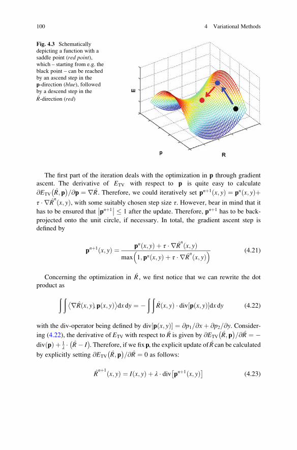
The first part of the iteration deals with the optimization in p through gradient

ascent. The derivative of ETV with respect to p is quite easy to calculate

@ETV R; p� �

@= p ¼ rR. Therefore, we could iteratively set pnþ1 x; yð Þ ¼ pn x; yð Þþτ � rRn

x; yð Þ, with some suitably chosen step size τ. However, bear in mind that it

has to be ensured that pnþ1�� 1 after the update. Therefore, pnþ1 has to be back-

projected onto the unit circle, if necessary. In total, the gradient ascent step is

defined by

pnþ1 x; yð Þ ¼ pn x; yð Þ þ τ � rRnx; yð Þ

max 1; pn x; yð Þ þ τ � rRnx; yð Þ

� � (4.21)

Concerning the optimization in R , we first notice that we can rewrite the dot

product as

ð ðrR x; yð Þ; p x; yð Þ�

dx dy ¼ �ð ð

R x; yð Þ � div p x; yð Þ½ �dx dy (4.22)

with the div-operator being defined by div p x; yð Þ½ � ¼ @p1 @x= þ @p2 @y= . Consider-

ing (4.22), the derivative of ETV with respect to R is given by @ETV R; p� �

@= R ¼ �div pð Þ þ 1

λ � R� I� �

. Therefore, if we fixp, the explicit update of R can be calculated

by explicitly setting @ETV R;p� �

@= R ¼ 0 as follows:

Rnþ1

x; yð Þ ¼ I x; yð Þ þ λ � div pnþ1 x; yð Þ� (4.23)

Fig. 4.3 Schematically

depicting a function with a

saddle point (red point),which – starting from e.g. the

black point – can be reached

by an ascend step in the

p-direction (blue), followedby a descend step in the

R-direction (red)


Altogether, the following update rules are to be performed in alternation:

pnþ1 x; yð Þ ¼ pn x; yð Þ þ τ � rRnx; yð Þ

max 1; pn x; yð Þ þ τ � rRnx; yð Þ

� �

Rnþ1

x; yð Þ ¼ I x; yð Þ þ λ � div pnþ1 x; yð Þ� (4.24)

where 0 < τ � 1 8λð Þ= and the iteration is initialized by R0x; yð Þ � I x; yð Þ and

p0 x; yð Þ � 0; 0½ � (i.e., set p to the zero vector for each position x; yð Þ ). Thedenominator on the right-hand side of the first line of (4.24) ensures that the

magnitudes of the vector field pnþ1 x; yð Þ are always smaller than 1 or equal to 1.

Finally, the iteration converges to the desired solution R� x; yð Þ . Convergence is

indicated, for example, if the change of the energyEnþ1TV � En

TV falls below a certain

threshold ε. Some implementations just perform a fixed number of iterations and

assume that a more or less steady state has been reached. The general proceeding is

illustrated in the flowchart of Fig. 4.4.

If we want to implement (4.24) numerically, we move from the continuous to the

discrete domain. To this end, we have to define the finite versions of the gradient

and divergence operators. There are several ways to calculate the gradient and

divergence numerically. Because (4.22) has to be satisfied in the discrete domain as

well, the gradient is calculated by forward differences, whereas the divergence is

calculated by backward differences. This yields the following simple calculation

rules:

rR x; yð Þ ¼ Rx

Ry

� � Rx ¼ R xþ 1; yð Þ � R x; yð Þ if 0 < x < W0 x ¼ W

�

Ry ¼ R x; yþ 1ð Þ � R x; yð Þ if 0 < y < H0 y ¼ H

� (4.25)

no

Initialization:R0 = I ; p0 =0

Update Rwith explicitminimization

S

E

yes

Convergence ?

Update pby gradient

ascent

Fig. 4.4 Flowchart of the variational optimization of the ROF model


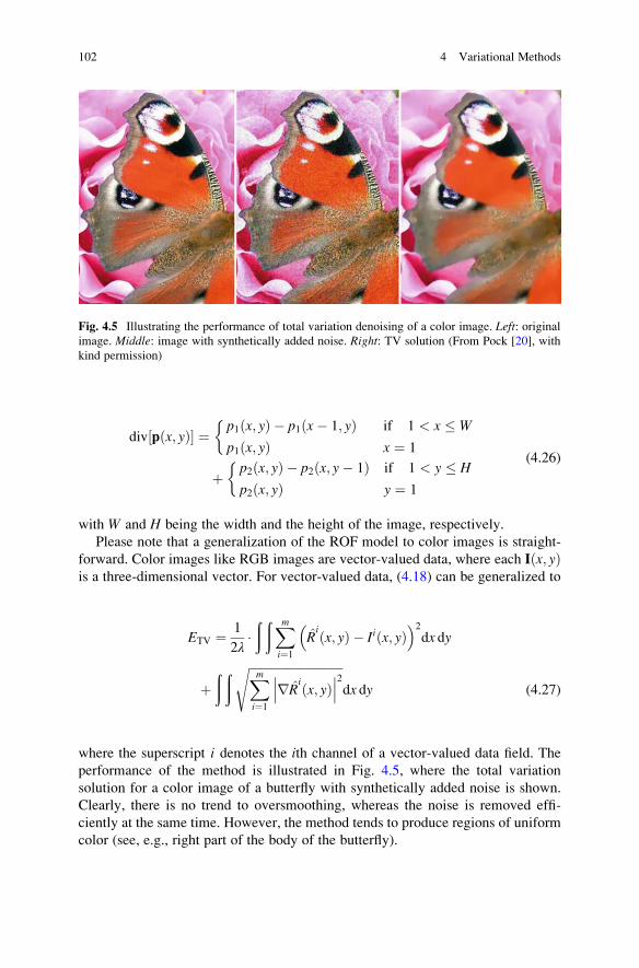
div p x; yð Þ½ � ¼ p1 x; yð Þ � p1 x� 1; yð Þ if 1 < x � W

p1 x; yð Þ x ¼ 1

�

þ p2 x; yð Þ � p2 x; y� 1ð Þ if 1 < y � H

p2 x; yð Þ y ¼ 1

� (4.26)

with W and H being the width and the height of the image, respectively.

Please note that a generalization of the ROF model to color images is straight-

forward. Color images like RGB images are vector-valued data, where each I x; yð Þis a three-dimensional vector. For vector-valued data, (4.18) can be generalized to

ETV ¼ 1

2λ�ð ðXm

i¼1Rix; yð Þ � Ii x; yð Þ

� �2

dx dy

þð ð ffiffiffiffiffiffiffiffiffiffiffiffiffiffiffiffiffiffiffiffiffiffiffiffiffiffiffiffiffiffiffi

Xm

i¼1rRi

x; yð Þ��

��2

sdx dy (4.27)

where the superscript i denotes the ith channel of a vector-valued data field. The

performance of the method is illustrated in Fig. 4.5, where the total variation

solution for a color image of a butterfly with synthetically added noise is shown.

Clearly, there is no trend to oversmoothing, whereas the noise is removed effi-

ciently at the same time. However, the method tends to produce regions of uniform

color (see, e.g., right part of the body of the butterfly).

Fig. 4.5 Illustrating the performance of total variation denoising of a color image. Left: originalimage. Middle: image with synthetically added noise. Right: TV solution (From Pock [20], with

kind permission)


Pseudocode

function denoiseTotalVariation (in Image I , in algoparameters τ and λ , in convergence criterion ε , outreconstructed image R�)

// initializationn 0

R0 I

p0 0

// main optimization looprepeat

// gradient ascend in p-direction (R fixed)for y ¼ 0 to H � 1

for x ¼ 0 to W � 1

calculate rRnx; yð Þ according to (4.25)

set pnþ1 x; yð Þ according to (4.21) // update pnext

next

// explicit minimization in R-direction (p fixed)for y ¼ 0 to H � 1

for x ¼ 0 to W � 1

calculate div pnþ1 x; yð Þ½ � according to (4.26)

set Rnþ1

x; yð Þ according to (4.23) // update Rnext

next

calculate energy Enþ1TV according to (4.18)

n nþ 1

until EnTV � En�1

TV < ε // convergence criterion

R� Rn

4.3.3 Efficient Implementation of TV Methods

Despite there is a considerable amount of theoretical background knowledge

necessary in order to develop the proceeding for finding the solution of the TV

problem formulation of denoising, the numerical procedure itself is very straight-

forward to calculate. In fact, the nature of the calculations being necessary when the

iterative update rule of (4.24) is applied makes the method perfectly suitable for an

implementation on massively parallel hardware such as graphical processing units

(GPUs). As a result, the method can be implemented very efficiently and thereby

the calculations are accelerated significantly.


So why do TV methods benefit so much from GPU implementations? Let’s take

a look at (4.24) from this perspective. We don’t want to go into detail here on how

to program GPUs efficiently (see, e.g., [11] for a good and easy to understand

introduction). For now, it suffices to mention that the main point is that for a good

performance on a GPU, it has to be possible to calculate the result for each pixel

separately, because then there will always be enough data to calculate for every

processing entity of the GPU. This is true for both left-hand sides of (4.24), as the

updated value of each pixel does not depend on the updated value of any other

pixel. This also becomes evident in the pseudocode implementation, where the

updates are performed in the inner part of the loops iterating over the image plane.

As a consequence, it is possible to calculate the updates of each pixel in a separate

thread, which results in hundreds of thousands or even more threads for typical

image sizes, which are definitely enough to use the massively parallel hardware at

full capacity.

Moreover, the numerical operations necessary to calculate the updated value of

one pixel are rather simple and therefore very fast to calculate. Apart from some

multiplications and additions (and one max-operation), the gradients of Rnas well

as the div �ð Þ-operators with argumentpnþ1 x; yð Þhave to be calculated for each pixel.Both of them depend on only a small amount of input data and can be calculated

with just a few multiplications and additions. Additionally, the whole iteration can

be processed on the GPU, which avoids extensive copy of data between CPU and

GPU, which can occur in algorithms where only parts of the calculation are done on

the GPU and the rest on the CPU.

Please note that in spite of being derived for the rather special case of image

denoising, the ROF model can be reused as a building block in total variation

solutions for quite a variety of vision problems, such as:

• Deconvolution (see, e.g., [19])

• Optical flow calculation (see, e.g., [32])

• Multi-view stereo reconstruction (see, e.g., [12])

• Segmentation/multi-class labeling (see, e.g., [14])

• Globally consistent depth estimation from 4D light fields (see, e.g., [28])

Without going into details, these methods use variants of the iterative TV update

of (4.24) or contain it as a building block next to other calculations, and, therefore,

all benefit from its particular suitability for a GPU implementation. Consequently,

TV methods have been a very active area of research in the last few years. One of

these examples, namely, optical flow calculation, will be presented in the following.

4.3.4 Application: Optical Flow Estimation

In this section, we will learn more about how total variation-based approaches can

be utilized for the optimization of other vision problems. In particular, we will

examine how a variant of the TV-based ROF model can be used to estimate the

optical flow between two images.


Consider a scenario where we have two images I0 and I1 which both show

the same scene, which contains moving objects like animals, cars, pedestrians, etc.

If I0 and I1 are acquired at different points of time, the moving objects will appear

at different locations in both images, whereas the background remains static. As

displacement can take place in two directions (x and y), the movement (which can be

different for each pixel) can be expressed as a two-dimensional vector u x; yð Þ ¼u1 x; yð Þ; u2 x; yð Þ½ �T for each pixel. Altogether, the movement is described by the

two-dimensional vector field u, which is called optical flow.Taking the two images I0 and I1 as input, we can deriveuby assigning a position

x of I0 to that position xþ u xð Þð Þ of I1 depicting the same scene element. By doing

this for every pixel, we can derive the optical flow u for the whole image plane.

This is another example of an ill-posed problem, because in addition to the

unknowns u x; yð Þ, I0 and I1 are also influenced by unknown perturbations like

noise and blur, which also have to be considered somehow during the optimiza-

tion process if their influence should be suppressed. In total, we again have more

unknowns than observations, which results in ill-posedness.

In their seminal work, Horn and Schunck therefore suggested a variational

approach in order to estimate u [8], which minimizes an energy being based on a

data term as well as a regularizer. Because their data fidelity term penalizes

deviations in a quadratic way, their method is not robust with respect to outliers

in the data. Therefore, the authors of [32] suggested a total variation-based energy

functional as follows:

ETVL1 ¼ λ �ð ð

I0 xð Þ � I1 xþ u xð Þð Þj jdxþð ðru1 xð Þj j þ ru2 xð Þj jdx (4.28)

The regularization part of this energy consists of the sum of the total variation of

the two components of the vector field u. The usage of TV here ensures that the

optimization preserves discontinuities in the flow field, which typically occur at the

borders of moving objects. The data fidelity term sums up the differences between

the intensity values I0 xð Þ in the first image and the intensities at their assumed

corresponding positions I1 xþ u xð Þð Þ in the second image. Because here the data

term utilizes L1 norms, too, the impact of data outliers is reduced compared to the

model of Horn and Schunck. We therefore speak of TVL1 optimization (instead of

TVL2, as used in the ROF model, where the data term contains a sum of squares).

If we want to find the minimizer u� of (4.28), we first have to notice that in

contrast to the ROF model, the data-driven part does not directly depend on u, as uonly appears in the argument of I1 xþ u xð Þð Þ. Explicit differentiations of the data

term with respect tou are therefore not possible at the moment. This can be resolved

by applying a first-order Taylor approximation of the data term at the current

estimate u0 (i.e., the data term is linearized):

I1 xþ u xð Þð Þ ffi I1 xþ u0 xð Þð Þ þ u xð Þ � u0 xð Þ;rI1 xþ u0 xð Þð Þh i (4.29)


with �h i denoting the dot product. Now we can rewriteETVL1 as follows (for brevity,

we will just write u instead of u xð Þ):

ETVL1 ¼ λ �ð ð

I0 xð Þ � I1 xþ u0ð Þ � u� u0;rI1 xþ u0ð Þh ij jdx

þð ðru1j j þ ru2j jdx ð4:30Þ

The next problem is that here both parts of ETVL1 are not continuously differen-

tiable, because the data term contains the L1 norm, too. This problem can

be handled well by formulating a convex approximation of (4.30). Convexity

can be obtained by decoupling the data term and the regularizer, which currently

both depend on u . To this end, an auxiliary variable v can be introduced,

which should approximate u. Therefore, v is a 2D vector field of the same size as

u. When replacing uwith v in the data term as well as abbreviating the data term by

ρ vð Þ ¼ I0 xð Þ � I1 xþ v0ð Þ � v� v0;rI1 xþ v0ð Þh i; a convex approximation of

(4.30) can be formulated by

ETVL1 ¼ λ

ð ðρ vð Þj jdxþ 1

2θ

ð ðu1 � v1ð Þ2 þ u2 � v2ð Þ2dx

þð ðru1j j þ ru2j jdx (4.31)

Now the data residuals and the regularization term are decoupled. Through the

introduction of the middle term, solutions wherevdiffers much fromu are penalizedand therefore avoided. Typically, θ is chosen as a small constant and ensures that vstays close to u.

In the form of (4.31), the energy depends on bothu andv . Consequently, it has tobe minimized with respect to both variables when calculating the solution. This can

be done by an iterative scheme, where in the first step one variable is fixed and

(4.31) is minimized with respect to the other. After that, we fix the just optimized

variable and minimize (4.31) with respect to the previously fixed variable. These

two steps are performed in alternation until finally the scheme converges.

Let’s first take a look at how to optimize ETVL1 in the form of (4.31) with respect

touwhen v is fixed. As the data term ρ vð Þ does not depend on u any longer, it can beneglected during this step. We can now minimize ETVL1 with respect to each of the

two components of u in a separate step by calculating

minud

1

2θ

ð ðud � vdð Þ2dxþ

ð ðrudj jdx

� �(4.32)

with d 2 1; 2f g. Taking a closer look at (4.32), we can see that this is exactly the

ROF model, and, therefore, we can apply the same iterative procedure as previously


described in order to optimize it.1 Please note that this iteration does not have to

fully converge; in practice it turned out that good overall solutions can be obtained

by just performing a fixed small number of iterations each time when (4.32) is to be

optimized.

The second step of the general iterative proceeding deals with minimization of

(4.31) with respect to v when u is fixed. In that step we have to calculate

minv

λ �ð ð

ρ vð Þj jdxþ 1

2θ

ð ðu1 � v1ð Þ2 þ u2 � v2ð Þ2dx

� �(4.33)

which has the desirable property that it can be solved point-wise in the discrete

domain, i.e., for each pixel separately, because in its discrete version, the integral is

replaced by a sum and each summand just considers a single pixel. Observe that

(4.33) does not depend on any derivatives, which would involve neighboring pixels.

Therefore, the solution can be calculated very quickly and is particularly suited for

a GPU implementation as well. Without giving any details here, the solution of the

discretized version of (4.33) is given by

v x; yð Þ ¼ u x; yð Þ þλθ � rI1 x; yð Þ�λθ � rI1 x; yð Þ�ρ uð Þ rI1 x;yð Þ

rI1 x;yð Þj j2

if ρ uð Þ < �λθ rI1 x; yð Þj j2if ρ uð Þ > λθ rI1 x; yð Þj j2if ρ uð Þj j � λθ rI1 x; yð Þj j2

8><>:

(4.34)

This can be seen as a soft thresholding step, which bounds the distance betweenvandu in cases where the absolute value of the data-driven energy ρ uð Þ gets too large(first two cases of (4.34)). This way, it is ensured thatv stays close tou. Details of thederivation of (4.34) can be found in [20, 32].

The last thing to mention is that the linearization step of (4.29) might introduce

too large errors at positions where u xð Þ gets too large. Therefore, [32] suggests a

top-down approach, which first calculates a solution at a coarse level of pixel

resolution. Subsequently, this solution serves as a starting point and can be succes-

sively refined by increasing the resolution until full resolution is reached.

An example of the performance of the method can be seen in Fig. 4.6 for two

examples. In the left two rows, we can see two images of the same scene taken at

different points of time. Each of the two scenes contains moving objects on a static

background. The right images show the optical flow estimate, which is color-coded

such that the hue represents the direction of the flow, whereas the saturation

indicates its magnitude. All moving objects were captured correctly.

1 Actually, (4.32) describes two ROF models: one for u1 (where d ¼ 1) and one for u2 (where

d ¼ 2). Consequently, we have to perform two (separate) optimizations.


Pseudocode

function opticalFlowEstimationTVL1 (in Image I0, in Image I1,in max. downscale factor K, in algo parameters τ, λ and θ,in convergence criterion ε, out optical flow estimate u�)

// initialization

uK;0 0

vK;0 uK;0

// main iteration loop (controlling pixel resolution)for k ¼ K to 0 step -1

if k > 0 then

downscale I0 and I1 by factor 2k

end ifn 0// main optimization loop (at current resolution)repeat

// optimization of u with ROF model (v fixed)

calculate uk;nþ11 by optimizing the ROF model based on(4.32) with d ¼ 1 // with fixed small number of it.

calculate uk;nþ12 by optimizing the ROF model based on(4.32) with d ¼ 2 // with fixed small number of it.// point-wise optimization of v (u fixed)

for y ¼ 0 to H � 1ð Þ 2k

Fig. 4.6 Illustrating the performance of TVL1 optimization when estimating the optical flow

between two images. See text for details (From Zach et al. [32], with kind permission from

Springer Science and Business Media)


for x ¼ 0 to W � 1ð Þ 2k

calculate vk;nþ1 x; yð Þ according to (4.34)next

next

calculate energy Enþ1TVL1 according to (4.31)

n nþ 1

until EnTVL1 � En�1

TVL1 < ε // convergence criterionif k > 0 then

uk�1;0 upscale of uk;n (by factor of 2)

vk�1;0 upscale of vk;n (by factor of 2)end if

next

u� u0;n

4.4 MAP Image Deconvolution in a Variational Context

4.4.1 Relation Between MAP Deconvolutionand Variational Regularization

The proceeding to recoverR from observed image data I in consideration of the blurkernelK (see (4.6)) is referred to as deconvolution, and another example of applying

variational methods, as our goal, is to estimate some functions R and K. Dependingon whether the blur kernel K is known or not, we talk about blind deconvolutionðK is unknown; see, e.g., [13]) or non-blind deconvolution, respectively.

An early technique of blind deconvolution, given the observed image I , is to

perform a joint estimation of R and K through a MAP (maximum a posteriori)estimation, which means that the goal is to jointly maximize the probability of Rand K, given the image data I . As we will see shortly, there is an interesting link

betweenMAP estimation and the energy-based variational approach presented so far.

The quantityp R;K Ijð Þdescribes the (joint) probability distribution ofR andK afterobservation of the image data I and is therefore denoted as the posterior probabilityAs we want to maximize the posterior p R;K Ijð Þ in order to infer the original image,

this kind of maximization is referred to as maximum a posteriori estimation.

If we knew the probability distribution p R;K Ijð Þ, we could select R� andK� suchthat p R;K Ijð Þ is maximized, i.e., R�;K�ð Þ ¼ argmax

R;Kp R;K Ijð Þ, under consideration

of the observed data I . Unfortunately though, this distribution is usually not

known. A way out of this dilemma is the application of Bayes’ rule, which states

that p R;K Ijð Þ can be modeled by

p R;K Ijð Þ ¼ p I R;Kjð Þ � pðRÞ � pðKÞpðIÞ (4.35)

4.4 MAP Image Deconvolution in a Variational Context 109

The quantity p I R;Kjð Þ is a data-driven term and quantifies the probability that an

image observation I occurs given a specific model setting R;Kð Þ and is usually

denoted as the likelihood function. pðRÞ and pðKÞ denote PDFs independent of

observing any data and are called prior probabilities (or just prior). They represent

knowledge about the model which can be assumed without considering observed

data, e.g., we can assume that images with very high overall gradient strength are

not very likely.

For the moment, let’s assume that we don’t want to favor any specific kernel, i.e.,

pðKÞ is the same for every possible kernel. Moreover, when judging different R;Kð Þsettings during optimization, we always use the same input image I. Therefore,pðKÞand pðIÞ can be dropped.

Please note that it is much easier to model the likelihood p I R;Kjð Þ than the

posterior p R;K Ijð Þ. A natural choice for p I R;Kjð Þ can be derived from the fact that

p I R;Kjð Þ should be high ifP

K � R� Ij j is small (where � denotes the convolu-

tion operator), because it can be assumed that the observed data is closely related to

the ground truth. Please observe the relation to (4.7).

The prior pðRÞ can be set such that the probability is low when the overall

gradient is high (in accordance to (4.8)), because natural images are assumed to

contain many uniform or smoothly varying regions.

Because PDFs are often modeled as Gaussian distribution involving exponential

terms, it is more convenient to optimize the logarithm of the above function. Taking

the negative � log p R;K Ijð Þ½ � converts the optimization problem into the following

minimization task:

R�;K�ð Þ ¼ argmin � log p R;K Ijð Þ½ �ð Þ argmin � log p I R;Kjð Þ½ � � log pðRÞ½ �ð Þ(4.36)

The term � log p R;K Ijð Þ½ � can be regarded as another representation of the

energy E defined in (4.9). Hence, � log p I R;Kjð Þ½ � and � log pðRÞ½ � can be

interpreted as Ed and Es , respectively. Therefore, MAP estimation in this context

is equivalent to a regularization-based variational approach utilizing an energy

functional consisting of two terms. In the MAP context, the likelihood is related

to a data-driven energy, whereas the priors act as regularization terms (which are

often smoothing terms). In other words, a MAP estimation in the form of (4.36) can

be considered as one way of performing variational optimization. As with the

previous section, the prior should help to overcome ill-posedness.

4.4.2 Separate Estimation of Blur Kerneland Non-blind Deconvolution

Observe that a joint estimation of R�;K�ð Þ with the MAP criterion usually fails,

mainly because the choice of the prior, which penalizes sharp edges (which


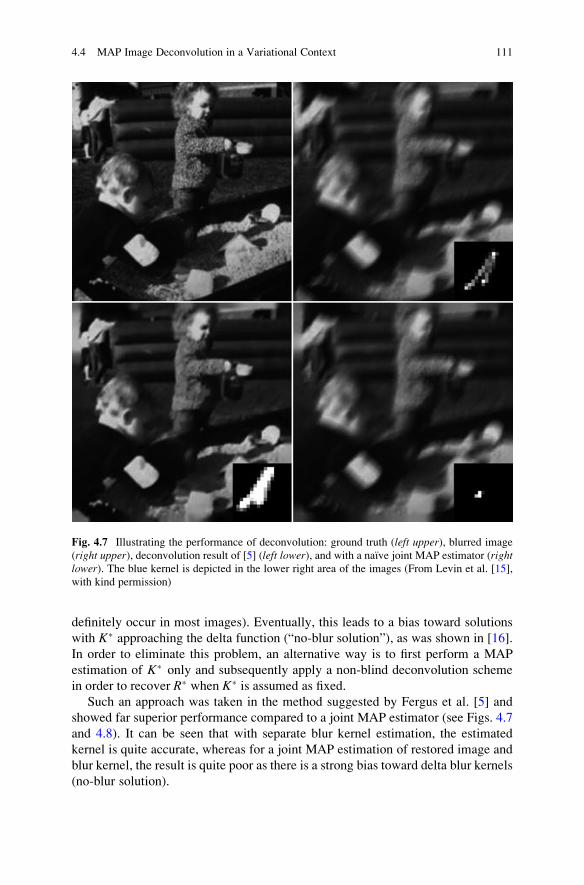
definitely occur in most images). Eventually, this leads to a bias toward solutions

with K� approaching the delta function (“no-blur solution”), as was shown in [16].

In order to eliminate this problem, an alternative way is to first perform a MAP

estimation of K� only and subsequently apply a non-blind deconvolution scheme

in order to recover R� when K� is assumed as fixed.

Such an approach was taken in the method suggested by Fergus et al. [5] and

showed far superior performance compared to a joint MAP estimator (see Figs. 4.7

and 4.8). It can be seen that with separate blur kernel estimation, the estimated

kernel is quite accurate, whereas for a joint MAP estimation of restored image and

blur kernel, the result is quite poor as there is a strong bias toward delta blur kernels

(no-blur solution).

Fig. 4.7 Illustrating the performance of deconvolution: ground truth (left upper), blurred image

(right upper), deconvolution result of [5] (left lower), and with a naıve joint MAP estimator (rightlower). The blue kernel is depicted in the lower right area of the images (From Levin et al. [15],

with kind permission)


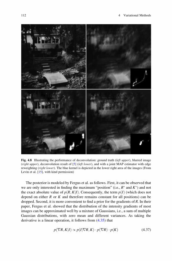
The posterior is modeled by Fergus et al. as follows. First, it can be observed that

we are only interested in finding the maximum “position” (i.e., R� and K�) and not

the exact absolute value of p R;K Ijð Þ. Consequently, the term pðIÞ (which does not

depend on either R or K and therefore remains constant for all positions) can be

dropped. Second, it is more convenient to find a prior for the gradients of R. In theirpaper, Fergus et al. showed that the distribution of the intensity gradients of most

images can be approximated well by a mixture of Gaussians, i.e., a sum of multiple

Gaussian distributions, with zero mean and different variances. As taking the

derivative is a linear operation, it follows from (4.35) that

p rR;K Ijð Þ / p I rR;Kjð Þ � p rRð Þ � pðKÞ (4.37)

Fig. 4.8 Illustrating the performance of deconvolution: ground truth (left upper), blurred image

(right upper), deconvolution result of [5] (left lower), and with a joint MAP estimator with edge

reweighting (right lower). The blue kernel is depicted in the lower right area of the images (From

Levin et al. [15], with kind permission)


The likelihood p I rR;Kjð Þ can be modeled by a Gaussian distribution with mean

rR � K and variance σ2 (which denotes the image noise). As already mentioned,

p rRð Þ is modeled by a mixture of C zero-mean Gaussians , where

wc is a weighting term and vc denotes the variance. Hence, denotes

the Gaussian probability distribution forrR, given zero mean and variance vc. Bothwcand vc can be specified in advance by evaluating training images, i.e., p rRð Þ isestimated based on a representative image set and it is assumed that this gradient

distribution is also valid for the images to be restored.

The prior pðKÞ should favor sparse kernels, i.e., only a small proportion of the

elements of K should differ significantly from zero. Therefore, a mixture of

exponential distributions is chosen: with for

x � 0. The constraint that x is not allowed to take negative values relates to the factthat all elements ofK have to be nonnegative. To sum it up, (4.37) can be rewritten as

ð4:38Þ

where i indexes over the pixels of the image and j over the elements of the kernel K.Observe that the probabilities for different pixels are modeled as being independent;

hence, the product of the contributions of the individual pixels is calculated in (4.38).

The exact optimization algorithm applied by Fergus et al. is quite advanced and

beyond our scope here, so it will be just roughly outlined. As a direct optimization

of (4.38) (or the negative logarithm of (4.38)) did not yield the desired results,

the authors of [5] employed a variational Bayesian approach which computes

an approximation of the MAP. This approximation distribution is the product

q rR;Kð Þ ¼ q rRð Þ � qðKÞ . Moreover, they built a cost function representing the

distance between the approximation and the true posterior, which was set to the

Kullback-Leibler divergence. The minimum of this cost function yields the desired

estimate K� of the blur kernel. The main advantage of using the Kullback-Leibler

divergence here is that, in its closed form, it can be expressed as simple as by a sum

of several expectations, where each expectation relates to a specific design variable.

Details can be found in [5, 9, 17] as well as the references therein.

In a subsequent step, the reconstructed image R� can be found using the well-

knownRichardson-Lucy algorithm [21] as a classical non-blind deconvolution scheme.

4.4.3 Variants of the Proceeding

The method of Shan et al. [23] takes a modified approach of the successive

blur kernel estimation and non-blind deconvolution. It introduces two major

modifications:


• Reweighting of the gradients when calculating � log pðRÞ½ � : Similar to the

weighting factors sx x; yð Þ and sy x; yð Þ of (4.11), the gradients in R can be

weighted according to the gradients of I . If the sensed data I exhibits a high

gradient at a certain position a; bð Þ, the penalty of high gradients atR a; bð Þ can belowered. As a consequence, such an edge reweighting favors solutions which are

piecewise constant. This is desirable, because this reduces so-called ringing

artifacts, which are sinusoidal intensity modulations and are encountered very

often in blind deconvolution. As can be seen in the lower right image of Fig. 4.8,

this reweighting enables the joint estimator to be pulled away from the no-blur

solution (compared to joint MAP estimation without gradient reweighting;

cf. lower right image of Fig. 4.7) but still is far from the optimum.

• Iterative update of the likelihood: Shan et al. proposed an iterative estimation of

R� and K�, i.e., R� and K� are updated in alternation until convergence is

achieved. Additionally, the likelihood term is weighted differently at each

iteration k . More specifically, they introduced a weighting factor λ for the

likelihood term � log p I R;Kjð Þ½ �. As the iteration proceeds, λ changes its value.It is advisable to start with low λ values in early iterations and then successively

increase λ as k increments. As was shown in [16], low values of λ favor solutionswith kernel estimatesK�;k being much closer to the true kernelK compared to the

naıve joint MAP estimator. As a consequence, there is a much better chance to

avoid being stuck at a local minimum if λ is set to low values in early iteration

steps. Because the updated solutions R�;k;K�;k� �

are searched only locally at

each iteration step, the algorithms stays at a local minimum where the current

kernel estimation K�;k is close to the true K. This should also hold when λ takeshigher values.

As can be seen in Fig. 4.9, quite impressive results can be obtained for blind

deconvolution. However, the algorithm needs a rough initial kernel estimate K�;0.The deconvolution algorithms presented so far assume that the blur kernel K is

uniform for the entire image. However, this might be not true. AsWhyte et al. found

out [30], pixel displacements caused by camera rotation during exposure typically

are larger than displacements by camera translation, at least for consumer cameras.

Camera rotation, however, causes non-uniform blur, i.e., it varies across the image

plane, as illustrated in Fig. 4.10. Therefore, Whyte et al. suggest a modified

proceeding capable of removing non-uniform blur caused by camera rotation.

The displacement of an image point x caused by camera rotation can be modeled

by a projective transformation, which can be written as a linear system of equations

when homogeneous coordinates are used:

x0 ¼s � x0s � y0s

24

35 ¼ H � x ¼

h11 h12 h13h21 h22 h23h31 h32 1

24

35 �

xy1

24

35 (4.39)

Homogeneous coordinates can be transformed back into inhomogeneous

coordinates by dividing all elements by the last element of the vector, i.e., by the


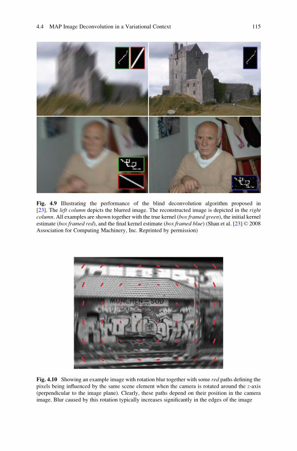
Fig. 4.9 Illustrating the performance of the blind deconvolution algorithm proposed in

[23]. The left column depicts the blurred image. The reconstructed image is depicted in the rightcolumn. All examples are shown together with the true kernel (box framed green), the initial kernelestimate (box framed red), and the final kernel estimate (box framed blue) (Shan et al. [23] © 2008

Association for Computing Machinery, Inc. Reprinted by permission)

Fig. 4.10 Showing an example image with rotation blur together with some red paths defining thepixels being influenced by the same scene element when the camera is rotated around the z-axis(perpendicular to the image plane). Clearly, these paths depend on their position in the camera

image. Blur caused by this rotation typically increases significantly in the edges of the image


scale factor s used in (4.39). The matrix H defines the projective transformation

specified by eight independent parameters. If camera parameters are known, the

matrix H can be replaced by a product of the camera’s internal calibration matrix

and a rotation matrix with only three degrees of freedom, which relate to the

rotations about the three axes of a 3D space.

If we consider a non-uniformly blurred image where camera rotation follows a

certain profile during exposure, the exposure time can be partitioned into T small

time slots t. Within each time slot, the camera rotation can be assumed constant and

thus is defined by a single matrixHt. As a result, the observed image I is a summation

of T versions of the transformed non-blurred image R, plus a noise term n:

I xð Þ ¼XT

t¼1R Ht � xð Þ þ n (4.40)

As we do not know the temporal progression of camera rotation, the observed

image can be modeled by the weighted summation over all possible camera

rotations θ, where each weight wθ is proportional to the amount of time the camera

stays at rotation θ:

I xð Þ ¼X

θ

wθR Hθ � xð Þ þ n (4.41)

Consequently, all wθ can be combined into a blur kernelW, which now consists

of quantities specifying the influence of several rotated versions of the unblurred

image. For the deconvolution procedure, Whyte et al. used the framework of [5],

i.e., they first calculate an estimation W� of the blur kernel using the variational

method of [5] (adapted to non-uniform blur) and subsequently estimate the

reconstructed image R� with the Richardson-Lucy algorithm [21].

In order to illustrate the performance of the method, let’s take a look at Fig. 4.11:

Here, a street scene (upper left) is blurred by camera rotation about the z-axis duringexposure (upper right). The increased influence of the blur in the edges of the image

is clearly visible. The deblurring result of Fergus et al. is shown in the lower left

image, whereas the result of the non-uniform algorithm proposed by Whyte et al. is

shown in the lower right image. Clearly, the non-uniform deconvolution performs

much better for this example, especially in the corners of the image.

4.5 Active Contours (Snakes)

Another application where variational optimization can be applied are so-called

active contours, which are also termed snakes. The following section, which

introduces into the concept of active contours and describes lesion detection in


skin cancer images as an example application, is a modified version of Sect. 6.2

of [27].

Snakes are parametric curves and can be used, for example, as a description of

the outer shape of an object. In such cases the parameters of the curve should be

chosen such that the curve follows the object contour, i.e., it proceeds along the

border of the object to the background. A parametric curve v s;φð Þ can be written as

v s;φð Þ ¼ x s;φð Þ; y s;φð Þ½ � (4.42)

with φ being a vector of model parameters specifying the curve and s being a scalarmonotonously increasing from 0 to 1 as the curve is traversed, which is often

referred to as the arc length parameter. The run of the curve should approximate

the object contour as good as possible. As the curve is represented by a functional

relationship, a specific curve v s;φð Þ being suitable for describing an object shape

accurately can be found by means of variational optimization. Numerical

implementations aim at calculating the xi; yi½ �-positions for sampled values si ofthe arc length parameter s.

Fig. 4.11 Illustrating the performance of the non-uniform deconvolution presented in [30]

(see text for details) (© 2010 IEEE. Reprinted, with permission, from Whyte et al. [30])

4.5 Active Contours (Snakes) 117

http://dx.doi.org/10.1007/978-1-4471-5283-5_6

4.5.1 Standard Snake

4.5.1.1 Main Idea

Snakes have initially been proposed by Kass et al. [10] as a method of detecting

contours of deformable objects. They behave like an elastic band which is pulled to

the object contour by forces. The run of the curve/band is iteratively updated, and

eventually it should converge to the outer shape of the object being searched. The

forces affecting the snake are represented by an energy functional, which is iteratively

minimized.As a result, theminimizing argument specifies the updated curve positions.

During energy minimization the snakes change their location dynamically, thus

showing an active behavior until they reach a stable position being conform with

the object contour. For this reason they are also called active contour models. The

“movement” of the curve as the iteration proceeds reminds of snakes, which

explains the name. See e.g. [18] for a good introduction.

According to Kass et al. [10] the energy functional E accounts for multiple

influences and can be written as

E ¼Z1

0

Eint v s;φð Þð Þ þ Ed v s;φð Þð Þ þ Eext v s;φð Þð Þds (4.43)

Taking a closer look at (4.43), we can see that the total energy consists of three

components, which can be described as follows:

• Eint denotes the internal energy, which exclusively depends on v s;φð Þ, i.e., it isindependent of the observed image. Eint plays the role of a smoothness

constraint and helps to enforce that the run of the curve is smooth. To this

end, Eint is influenced by derivative information. More specifically, it depends

on the first- and second-order derivatives ofv s;φð Þwith respect tos. Consideringthe first-order derivative should exclude discontinuities, whereas second-order

information helps punishing curves containing sections of high curvature. In

this context, curvature can be interpreted as a measure of the energy which is

necessary to bend the curve.

• The data-driven term Ed measures how well the curve fits to the image data. The

curve should be attracted by local intensity discontinuities in the image

(locations with high gradients), because usually the object brightness differs

from the background intensity, and, therefore, we should observe some rapid

intensity changes at the object borders.

• The external constraints Eext aim at ensuring that the snake should remain near

the desired minimum as the iterative optimization proceeds. This can be

achieved by user input (e.g., when Eext is based on the distance of the curve to

user-selected “anchor points,” which are supposed by the user to be located on

the object contour) or by feedback of a higher-level scene interpretation method,

which could be run subsequently.


During optimization, the curve has to be estimated numerically. To this end, it is

sampled at a certain number of control points. Now, the task is to adjust the

positions of these control points such that the energy functional E reaches a

minimum. The appropriate optimization procedure is outlined in the following,

details can be found in the appendix of [10].

4.5.1.2 Optimization

As already mentioned, the internal energy, which acts as a smoothness constraint, is

usually modeled by a linear combination of the first- and second-order derivatives

of v s;φð Þ with respect to s:

Eint ¼ 1

2� α vs s;φð Þj j2 þ β vss s;φð Þj j2h i

(4.44)

Here, the parameters α and β determine the relative influence of the first- and

second-order derivative (which are denoted byvs andvss, respectively). The purposeof the two terms of (4.44) is to punish discontinuities and high curvature parts,

respectively. If β is set to 0, the curve is allowed to contain corners. It is possible tomodel α and β dynamically dependent on s or statically as constants.

Concerning the data-driven term, Ed should take smaller values at points of

interest, such as edge points. Consequently, the negative gradient magnitude is a

natural measure forEd. However, object borders usually lead to high gradient values

(and therefore large negative values of Ed) only within a very limited area in the

surrounding of the border. As a result, the convergence area, where the curve is

driven in the right direction, is usually very limited for this choice of Ed. It can be

increased, though, by utilizing a spatially blurred version of the gradient magnitude.

To this end, a convolution of the image content with a Gaussian kernelG x; y; σð Þ isapplied:

Ed x; yð Þ ¼ � r G x; y; σð Þ � I x; yð Þ½ �j j2

with G x; y; σð Þ ¼ 1ffiffiffiffiffi2πp

σ� e� x2þy2ð Þ 2σ2= (4.45)

where r and � denote the gradient and convolution operator, respectively.

As far as the external constraintsEext are concerned, they are often set to zero and

therefore aren’t considered any longer in this section.

As already said, the minimization of the energy functional is usually performed

without explicit calculation of the model parameters φ of the curve. Instead,

the curve position is optimized at N discrete positions v sið Þ ¼ x sið Þ; y sið Þ½ � withi 2 1; . . . ;N½ � and siþ1 ¼ si þ Δs. Δs denotes a suitably chosen step size. In other

words, the optimization task is to estimate the position of a discrete set of pointsv sið Þ.


If the internal and image constraints are modeled as described above and,

additionally, we assume that α and β are constants, the snake must satisfy a system

of two independent Euler equations in order to minimizeE. The Euler equations aredefined by

XN

i¼1αxss sið Þ þ βxssss sið Þ þ @Ed sið Þ

@x¼ 0

XN

i¼1αyss sið Þ þ βyssss sið Þ þ @Ed sið Þ

@y¼ 0

(4.46)

with xssðsÞ resp. yssðsÞ being the second-order derivative and xssssðsÞ resp. yssssðsÞ thefourth-order derivative of the components of v with respect to s . The desired

minimum is found if the left-hand side of the Euler equations is equal to zero. (4.46)

is derived from the fact that, at the optimum, the derivative of the total energy is

equal to zero: rE ¼ rEint þrEd � 0.

A solution of these partial differential equations can be found numerically by

treating v as a function of time t and iteratively adjusting the discrete v si; tð Þ untilconvergence is achieved (see the appendix of [10] for details): starting from an

initial solution, an updated solution is calculated by approximating the derivatives

numerically at each time step tk, using the data at the current position of the sample

points.

The numerical approximation of the second-order derivatives of xssðsÞ and yssðsÞis given as follows:

xss sið Þ ¼ x si�1ð Þ � 2x sið Þ þ x siþ1ð Þyss sið Þ ¼ y si�1ð Þ � 2y sið Þ þ y siþ1ð Þ (4.47)

The fourth-order derivatives can be approximated by taking the second deriva-

tive of (4.47). Consequently, xssssðsÞ is approximated by

xssss sið Þ ¼ xss si�1ð Þ � 2xss sið Þ þ xss siþ1ð Þ¼ x si�2ð Þ � 4x si�1ð Þ þ 6x sið Þ � 4x siþ1ð Þ þ x siþ2ð Þ (4.48)

yssssðsÞ can be approximated analogously.

The derivatives @Ed sið Þ @x= and @Ed sið Þ @y= of the image constraint can be

calculated numerically by first performing a discrete convolution of I with a

Gaussian kernel G (whose size in pixel depends on the σ-parameter) yielding IGand then approximating the derivative by taking the differences between adjacent

pixels of IG in x-direction (or y-direction, respectively).


Through the usage of the numerical approximations defined by (4.47) and (4.48),

αxss sið Þ þ βxssss sið Þ is defined by β � x si�2ð Þ þ α� 4βð Þ � x si�1ð Þ þ 6β � 2αð Þ � x sið Þþ α� 4βð Þ � x siþ1ð Þ þ β � x siþ2ð Þ. Consequently, the Euler equations of (4.46) can

be written in matrix form:

A � xþ gx ¼ 0A � yþ gy ¼ 0

with

A ¼

6β � 2α α� 4β β 0 � � � 0 β α� 4β

α� 4β 6β � 2α α� 4β β 0 � � � 0 β

β α� 4β 6β � 2α α� 4β β 0 � � � 0

0 β α� 4β 6β � 2α α� 4β β 0 0

..

.0 . .

. . .. . .

. . .. . .

.0

0 � � � 0 β α� 4β 6β � 2α α� 4β β

β 0 � � � 0 β α� 4β 6β � 2α α� 4β

α� 4β β 0 � � � 0 β α� 4β 6β � 2α

266666666666664

377777777777775

x ¼

x s1ð Þx s2ð Þx s3ð Þ...

x sN�1ð Þx sNð Þ

2666666664

3777777775

y ¼

y s1ð Þy s2ð Þy s3ð Þ...

y sN�1ð Þy sNð Þ

2666666664

3777777775

gx ¼

@Ed s1ð Þ @x=

@Ed s2ð Þ @x=

@Ed s3ð Þ @x=

..

.

@Ed sN�1ð Þ @x=

@Ed sNð Þ @x=

2666666664

3777777775

gy ¼

@Ed s1ð Þ @y=

@Ed s2ð Þ @y=

@Ed s3ð Þ @y=

..

.

@Ed sN�1ð Þ @y=

@Ed sNð Þ @y=

2666666664

3777777775

(4.49)

Observe that for closed contours, the index of the points v sið Þ is “cyclic”, i.e.,v s0ð Þ ¼ v sNð Þ, v s�1ð Þ ¼ v sN�1ð Þ, and v sNþ1ð Þ ¼ v s1ð Þ.

The solution is now specified by the vectors x and y. At first glance, it seems that

it could be obtained by just solving the linear equation systems specified in (4.49).

However, in practice the solution has to be calculated iteratively. Please note that,

as long as the iteration has not converged yet, the right-hand sides of the Euler

equations don’t vanish, because the time derivative of the left-hand side is not zero. It

can be set to the difference between two successive steps of the iteration (multiplied

by a step size γ). Therefore, solving the linear system of equations defined in (4.49)

once is not enough. Instead, we have to employ an iterative scheme, where, unlike in

(4.49), the difference of the solution between two successive steps is considered, too.

Eventually, the suggested optimization method is a gradient descent algorithm.

In [10] it is suggested to use explicit Euler for the external forces (and therefore

evaluate gx and gy at position xt; ytð Þ) and implicit Euler for the internal energy (and

therefore multiply A by xtþ1 and ytþ1 ) (see the appendix of [10] for details).

Incorporating this in (4.49) yields the following update formulas:

A � xtþ1 þ gx xt; ytð Þ ¼ �γ � xtþ1 � xt� �

A � ytþ1 þ gy xt; ytð Þ ¼ �γ � ytþ1 � yt� � ð4:50Þ


These equations can be solved by matrix inversion, leading to

xtþ1 ¼ Aþ γ � Ið Þ�1 � xt � gx xt; ytð Þð Þytþ1 ¼ Aþ γ � Ið Þ�1 � yt � gy xt; ytð Þ

� � (4.51)

where I denotes the identity matrix. An iterative application of (4.51) dynamically

changes the course of the curve until finally it “snaps” to dominant edges and

convergence is achieved. The general flow of the method is illustrated in Fig. 4.12.

For constants α and β, the matrix A does not depend on position or time, and

therefore, the inverse Aþ γ � Ið Þ�1 can be calculated offline prior to the iterative

update of the control point positions. If α x; yð Þ and β x; yð Þ are location dependent,Ahas to be updated at each iteration step. As the matrix Aþ γ � Ið Þ has a

pentadiagonal structure (cf. (4.49)), its inverse can be calculated fast by an LU

decomposition of Aþ γ � Ið Þ.Figure 4.13 shows an example of fitting an initially circle-shaped curve to a

triangle form. The energy is minimized iteratively with the help of sample points

located on the current curve representation (indicated by green squares). The

images show the location of the sample points in the different steps of the iteration

(at start, after 6, 10, 15, 20, and the final iteration, from top left to bottom right). The

“movement” of each sample point as the iteration proceeds is shown by a specific

curve for each point (green and red curves).

Being a global approach, snakes have the very desirable property of being quite

insensitive to contour interruptions or local distortions. For this reason they are

often used in medical applications where, due to low SNR images, closed contours

often are difficult to obtain. A major drawback of snakes, though, is the fact that

they rely on a reasonable starting point of the curve (i.e., a rough idea where the

object border could be) for ensuring convergence to the global minimum of the

energy functional. If the starting point is located outside the convergence area of the

global minimum, the iteration might get stuck in a local minimum being arbitrarily

far away from the desired solution. Additionally, snakes sometimes failto penetrate

into deep concavities because the smoothness constraint is overemphasized in

those scenarios.

no

Calculate A

Update control points

on curveS

E

yesConvergence ?

Calc. Inverse(A+ g ·I)−1

Fig. 4.12 Flowchart of the variational optimization of active contour models


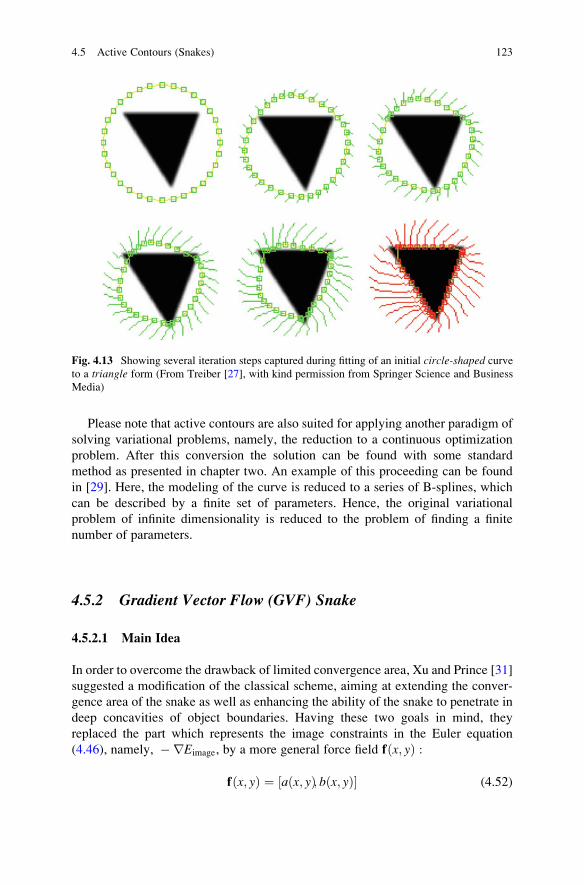
Please note that active contours are also suited for applying another paradigm of

solving variational problems, namely, the reduction to a continuous optimization

problem. After this conversion the solution can be found with some standard

method as presented in chapter two. An example of this proceeding can be found

in [29]. Here, the modeling of the curve is reduced to a series of B-splines, which

can be described by a finite set of parameters. Hence, the original variational

problem of infinite dimensionality is reduced to the problem of finding a finite

number of parameters.

4.5.2 Gradient Vector Flow (GVF) Snake

4.5.2.1 Main Idea

In order to overcome the drawback of limited convergence area, Xu and Prince [31]

suggested a modification of the classical scheme, aiming at extending the conver-

gence area of the snake as well as enhancing the ability of the snake to penetrate in

deep concavities of object boundaries. Having these two goals in mind, they

replaced the part which represents the image constraints in the Euler equation

(4.46), namely, �rEimage, by a more general force field f x; yð Þ :

f x; yð Þ ¼ a x; yð Þ; b x; yð Þ½ � (4.52)

Fig. 4.13 Showing several iteration steps captured during fitting of an initial circle-shaped curve

to a triangle form (From Treiber [27], with kind permission from Springer Science and Business

Media)


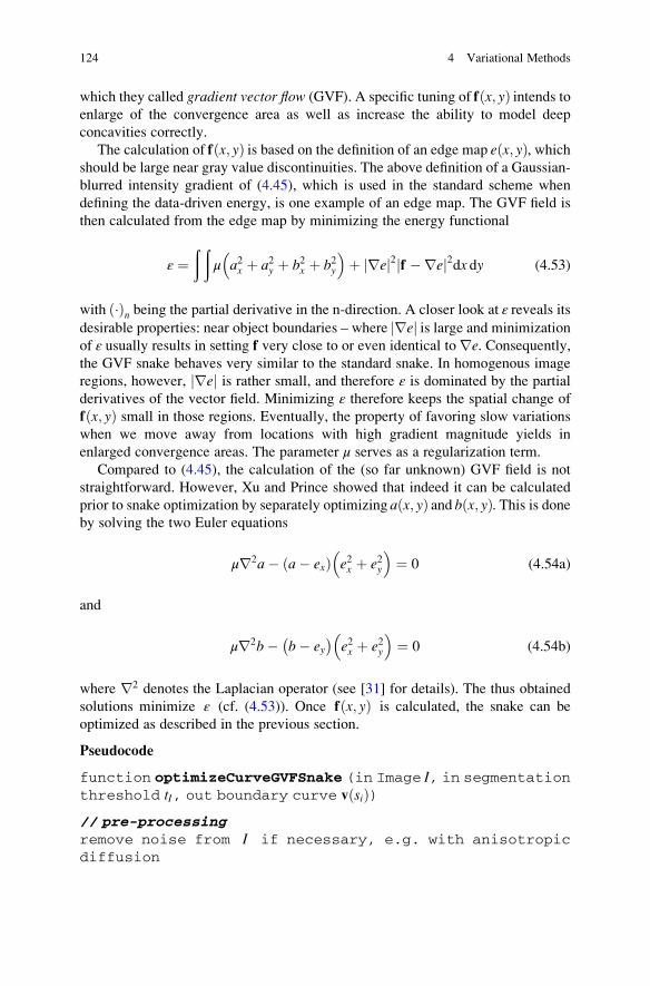
which they called gradient vector flow (GVF). A specific tuning of f x; yð Þ intends toenlarge of the convergence area as well as increase the ability to model deep

concavities correctly.

The calculation of f x; yð Þ is based on the definition of an edge map e x; yð Þ, whichshould be large near gray value discontinuities. The above definition of a Gaussian-

blurred intensity gradient of (4.45), which is used in the standard scheme when

defining the data-driven energy, is one example of an edge map. The GVF field is

then calculated from the edge map by minimizing the energy functional

ε ¼ð ð

μ a2x þ a2y þ b2x þ b2y

� �þ rej j2 f �rej j2dx dy (4.53)

with �ð Þn being the partial derivative in the n-direction. A closer look at ε reveals itsdesirable properties: near object boundaries – where rej j is large and minimization

of ε usually results in setting f very close to or even identical tore. Consequently,the GVF snake behaves very similar to the standard snake. In homogenous image

regions, however, rej j is rather small, and therefore ε is dominated by the partial

derivatives of the vector field. Minimizing ε therefore keeps the spatial change of

f x; yð Þ small in those regions. Eventually, the property of favoring slow variations

when we move away from locations with high gradient magnitude yields in

enlarged convergence areas. The parameter μ serves as a regularization term.

Compared to (4.45), the calculation of the (so far unknown) GVF field is not

straightforward. However, Xu and Prince showed that indeed it can be calculated

prior to snake optimization by separately optimizing a x; yð Þ and b x; yð Þ. This is doneby solving the two Euler equations

μr2a� a� exð Þ e2x þ e2y

� �¼ 0 (4.54a)

and

μr2b� b� ey� �

e2x þ e2y

� �¼ 0 (4.54b)

where r2 denotes the Laplacian operator (see [31] for details). The thus obtained

solutions minimize ε (cf. (4.53)). Once f x; yð Þ is calculated, the snake can be

optimized as described in the previous section.

Pseudocode

function optimizeCurveGVFSnake (in Image I, in segmentationthreshold tI, out boundary curve v sið Þ)// pre-processingremove noise from I if necessary, e.g. with anisotropicdiffusion


init of edge map e x; yð Þ with Gaussian blurred intensity gradi-ent magnitude of I (c.f. (4.45))calculate GVF field f x; yð Þ by solving Equation 4.54

// init of snake: segment the object from the background andderive the initial curve from its outer boundaryfor y ¼ 1 to height(I)

for x ¼ 1 to width(I)if I x; yð Þ � tI then

add pixel x; y½ � to object area oend if

nextnextget all boundary points b of osample boundary points b in order to get a discrete repre-sentation of parametric curve v si; 0ð Þ

// optimization (just outline, details see [10])t 0

calculate matrix inverse Aþ γ � Ið Þ�1calculate gx and gy according to positions defined by v si; 0ð Þrepeat

v si; tþ 1ð Þ result of update equation 4.51 // update curveupdate gx and gy according to the new positions defined by

v si; tþ 1ð Þt tþ 1

until convergence

4.5.2.2 Example: Lesion Detection

A medial image application of GVF snakes is presented by Tang [24], where the

GVF snake is incorporated in a lesion detection scheme for skin cancer images.

Starting from a color image showing one or more lesions of the skin, the exact

boundary of the lesion(s) is extracted (cf. Fig. 4.14). As can be seen in Fig. 4.14, the

images can contain more or less heavy clutter such as hairs or specular reflections in

the lesion region.

The method consists of four major steps:

1. Conversion of the original color image to a gray value image.

2. Noise removal by applying a so-called anisotropic diffusion filter: The basic ideaof anisotropic diffusion is to remove noise without blurring the gradients at true

object borders at the same time. To this end, the image is iteratively smoothed by

application of a diffusion process such that pixels with high intensity

(“mountains”) diffuse into neighboring pixels with lower intensity (“valleys”).


The main point is that this is done in an anisotropic way: diffusion should not

take place in the direction of dominant gray value gradients (thereby gradient

blurring is avoided!), but preferably perpendicular to it (where variations are

attributed to noise). Details can be found in [24] and are beyond the scope of

this book.

3. Rough segmentation by applying simple gray value thresholding: This step

serves for the estimation of reasonable starting regions for the subsequent

snake optimization.

4. Fine segmentation using a GVF snake. (To be correct, Tang [24] applied a

modified version aiming at making the method suitable for multi-lesion images

by modifying the force field, without giving any details here. In those cases the

snake has to be prevented to partly converge to one lesion and party to another

lesion in its vicinity.)

Especially to mention is that some restrictions of the standard snake scheme can

be overcome or at least alleviated by the usage ofGVF snakes. The additional degrees

of freedomobtained by the introduction ofmore general force fields can be utilized to

enlarge the convergence area or make the optimization more robust in situations

where the scene image contains multiple objects. On the other hand, the calculation

of the force field needs a second optimization procedure during recognition, which

increases the computational complexity of the method.

References

1. Bakushinsky A, Goncharsky A (1994) Ill-posed problems: theory and applications. Kluwer

Academic Publishers, Dordrecht. ISBN 978-0792330738

2. Briggs WL, Henson VE, McCormick SF (2000) A multigrid tutorial, 2nd edn. Society for

Industrial and Applied Mathematics, Philadelphia

Aniso.Diff.

Segmen-tation

GVF Calcu-lation

Snake Op-timization

Fig. 4.14 Illustrating the boundary extraction of the lesions of skin cancer images (after the initial

gray value conversion). The proceeding is explained in the text (From Treiber [27], with kind

permission from Springer Science and Business Media, with images taken from Tang [24], with

permission from Elsevier)


3. Chambolle A (2004) An algorithm for total variation minimization and applications. J Math

Imaging Vis 20:89–97

4. Chambolle A (2005) Total variation minimization and a class of binary MRF models. Int Conf

Energy Minimization Methods Comput Vision Pattern Recogn 5:136–152

5. Fergus R, Singh H, Hertzmann A, Rotweis S.T, Freeman W.T (2006) Removing camera shake

from a single photograph. In: SIGGRAPH, Boston

6. Fischen, J (1999) Introduction to the calculus of variations. http://online.redwoods.cc.ca.us/

instruct/darnold/staffdev/assignments/calcvarb.pdf. Published online



8. Horn K, Schunck B (1981) Determining optical flow. Artif Intell 17:185–203

9. Jordan M, Ghahramani Z, Jaakkola T, Saul L (1999) An introduction to variational methods

for graphical models. Mach Learn 38:183–233

10. Kass M, Witkin A, Terzopoulos D (1988) Snakes: active contour models. Int J Comput Vis

1:321–331

11. Kirk D.B, Hwu W.W (2012) Programming massively parallel processors: a hands-on

approach, 2nd edn. Morgan Kaufman, San Francisco. ISBN 978-0124159921

12. Kolev K, Klodt M, Brox T, Cremers D (2009) Continuous global optimization in multiview 3D

reconstruction. Int J Comput Vis 84(1):80–96

13. Kundur D, Hatzinakos D (1996) Blind image deconvolution. IEEE Signal Proc Mag

13(3):43–64

14. Lellman J, Becker F, Schnorr C (2009) Convex optimization for multi-class image labeling

with a novel family of total variation based regularizers. IEEE Int Conf Comput Vis

12:646–653

15. Levin A, Weiss Y, Durand F, Freeman WT (2009) Understanding blind deconvolution

algorithms. Extended Technical Report

16. Levin A, Weiss Y, Durand F, Freeman WT (2011) Understanding blind deconvolution

algorithms. IEEE Signal Proc Mag 33(12):2354–2367

17. Miskin J,MacKay DC (2000) Ensemble learning for blind image separation and deconvolution.

In: Girolani M (ed) Advances in independent component analysis. Springer, London

18. Nixon M, Aguado A (2007) Feature extraction and image processing. Academic Press,

New York. ISBN 978-0-12-372538-7

19. Oliveira JP, Bioucas-Dias JM, Figueiredo M (2009) Adaptive total variation image deblurring:

a majorization-minimization approach. Signal Process 89(9):1683–1693

20. Pock T (2008) Fast total variation for computer vision. PhD thesis, TU, Graz

21. Richardson WH (1972) Bayesina-based iterative method of image restoration. J Opt Soc

Am 62(1):55–59

22. Rudin LI, Osher S, Fatemi E (1992) Nonlinear total variation based noise removal algorithms.

Physica D 60:259–268

23. Shan Q, Jia J, Agarwala A (2008) High-quality motion deblurring from a single image.

ACM Trans Graphic 27(3)

24. Tang J (2009) A multi-direction GVF snake for the segmentation of skin cancer images.

Pattern Recogn 42:1172–1179

25. Terzopoulos D (1983) Multilevel computational processes for visual surface reconstruction.

Comput Vis Graph Image Process 24:52–96

26. Tikhonov AN, Arsenin VY (1997) Solutions of ill-posed problems. V.H. Winston,

Washington, DC. ISBN 047-099-1240

27. Treiber M (2010) An introduction to object recognition – selected algorithms for a wide

variety of applications. Springer, London. ISBN 978-1849962346

28. Wanner S, Goldluecke B (2012) Globally consistent depth labeling of 4D light fields. IEEE

Conf Comput Vis Pattern Recogn 25:41–48

References 127

http://online.redwoods.cc.ca.us/instruct/darnold/staffdev/assignments/calcvarb.pdf

http://online.redwoods.cc.ca.us/instruct/darnold/staffdev/assignments/calcvarb.pdf

29. Wesselink JW (1996) Variational modeling of curves and surfaces. PhD thesis, Technische

Universiteit Eindhoven

30. Whyte O, Sivic J, Zisserman A, Ponce J (2010) Non-uniform deblurring for shaken images.

IEEE Conf Comput Vision Pattern Recogn 23:491–498

31. Xu C, Prince JL (1998) Snakes, shapes and gradient vector flow. IEEE Trans Image Process

7(3):359–369

32. Zach C, Pock T, Bischof H (2007) A duality based approach for realtime TV-L1 optical flow.

In: Proceedings of the 29th DAGM conference on pattern recognition. Springer, Berlin,

pp 214–223


Chapter 5

Correspondence Problems

Abstract Quite numerous computer vision applications require an assignment of

the elements of a set of some extracted salient positions/descriptors to their

corresponding counterpart in a model set, at some point of their proceeding.

Examples are object recognition or image registration schemes. Because an exhaus-

tive evaluation of all possible combinations of individual assignments is infeasible

in terms of runtime, more sophisticated approaches are required, and some of them

will be presented in this chapter. Possible ways of speeding up the search are

applying heuristics, as done in the so-called search tree, or iterative approaches

like the iterative closest point method. A typical challenge when trying to find the

correct correspondences is the existence of a quite large number of outliers, e.g.,

positions being spoiled by gross errors. The straightforward approach of minimizing

total deviations runs into difficulties in that cases, and consequently, methods being

more robust to outliers are required. Examples of robust schemes are the random

sample consensus (RANSAC) or methods transforming the problem into a graph

representation, such as spectral graph matching or bipartite graph matching as done in

the so-called Hungarian algorithm.

5.1 Applications

Various applications comprise a step where the elements p1;m of one set of points

P1 ¼ p1;m;m 2 1; . . . ;M½ �� ; p1;m ¼ x1;m; y1;m

� �are to be matched to the elements

p2;n of a second point set P2 ¼ p2;n; n 2 1; . . . ;N½ �� ; p2;n ¼ x2;n; y2;n

� �, i.e.,

correspondences between the elements of P1 and P2 have to be established. This

task is described as the correspondence problem in literature. A correspondencecmn isfound if a certainp1;mmatches “best” top2;n. Somematching criteria will be described

below. A typical scenario is the matching of a data point set to a set of model points.

These correspondences can be used, for example, in image registration tasks,

where the content of different images is to be transformed into a single coordinate

system. A classical approach to registration tasks is to find corresponding points in



129

different images and, subsequently, utilize the positions of corresponding points for

an estimation of the parameters of an aligning transform, which maps the positions

of the first image into the corresponding position of the second image. A special

case of image registration is image stitching, where several images partly overlap.

By finding corresponding points in the overlapping part of two images, the trans-

formation between these two images can be estimated and the images can be

combined into a single image frame. With this technique, it is possible to assemble

a panorama image from multiple images. Correspondence problems can also arise

in stereo vision, where the displacement between corresponding points in two

images (which is called disparity) can be used to calculate the depth of the scene,

i.e., the z-distance from the scene to the stereo camera system.

Establishing correspondences can also be very helpful in the context of object

detection. Some object models consist of a spatial configuration of a set of points,

e.g., each point specifies the center position of a salient part of the object to be

found. By matching the set of characteristic points found in a query image to the

model point set, the so-called object pose can be revealed. Here, the object pose

denotes the set of parameters specifying the object location, e.g., x-/y-position,rotation, and scale.

Please note that in general the cardinality of the two point sets is different, i.e.,

M 6¼ N. In many applications, when correspondences between the points of two sets

are to be found, it is not necessary to establish one-to-one mappings between all

points in the two sets. There may be unmatched points in one of the sets, e.g., due to

background clutter (which introduces some extra points in one of the sets) or

occlusion (which makes some of the points invisible in one of the images). Some

applications also allow a point to be matched to multiple points in the other set

(so-called many-to-one mappings).

These examples illustrate the widespread appearance of correspondence

problems in computer vision. Therefore, let’s discuss how it can be solved in

more detail in this chapter. Obviously, the brute force approach of evaluating all

possible correspondences quickly becomes infeasible as the number of points

increases, because the number of possible correspondences grows exponentially

with the number of points. This exponential growth of possible assignments is

sometimes called the combinatorial explosion. Consequently, something more

elaborate has to be found in order to optimize the correspondences.

Before we take a closer look at the task of matching the points (i.e., finding the

correspondences), let’s first give a brief answer to the following two questions in

order to get a better understanding of the applications.

1. How can we find the points?

2. What criteria can be defined for matching?

For the first question, two different strategies are to be mentioned:

• Predefined filters: If we know what we search for, e.g., the outer shape of the

object parts, we can incorporate these shapes in the design of special filters,

which are applied to the image and yield high responses at positions where the

130 5 Correspondence Problems

image content fits to the filter design. If a filter is shifted pixel-by-pixel over the

search area and the filter response is calculated at each position, these responses

can be accumulated in a two-dimensional matching function. The local maxima

of the matching function being above a certain threshold indicate occurrences of

the searched object part and can be used as points to be matched. This proceed-

ing is well suited for industrial object detection (or inspection) applications,

where the object to be searched is known in advance. Hence, the filter can, e.g.,

be derived from CAD data.

• Interest point detection: A more generic proceeding is to search for the so-called

keypoints (also called interest points), which are to be located at highly infor-

mative positions. For example, the so-called Harris detector [8] aims at detecting

positions where the image intensity changes in both directions (x and y), i.e.,

there is a significant intensity gradient in x- as well as in y-direction. This

happens to be true at corners of objects, for example. In contrast to such points,

positions of uniform or slowly varying intensity only contain little information,

as they are very similar compared to their neighbors. Positions with significant

gradient in just one direction, e.g., at lines or edges, allow for accurate localiza-

tion in just one direction (at which the gradient points to), but not perpendicular

to it. For a more detailed introduction, the interested reader is referred to, e.g.,

[23] or [17].

As far as the matching criteria are concerned, there are two main approaches:

• Spatial configuration: If just the position of the points is available, we can evaluatewhich elements p2;n of P2 are spatially consistent to which elements p1;m of P1,

i.e., the spatial configuration defined by the matched points ofP2 has to be similar

to the one defined by their corresponding elements of P1 . What is meant to be

“similar” depends on the type of transformation a point set undergoes between the

first and the second image. For pure translations and Euclidean transformations,

for example, the distances between the points within a set have to be preserved.

Similarity transforms maintain the ratio of distances and so on.

• Descriptors: Here, the spatial position of the points is not the only source of

information which can be used for matching. In addition to the spatial positions, it

can be assumed that the appearance of a local image patch around one elementp2;nof P2 has to be similar to the appearance around its corresponding element p1;m of

P1. Therefore, an additional matching criterion can be defined by comparing the

image data of local patches around two matching candidates. Please note that in

many situations, we have to deal with effects like varying illumination conditions,

small deformations, or appearance change due to change of viewpoint. Therefore,

a comparison of the raw image data would lead to a quick decline of similarity in

the presence of those effects. A better approach is to derive a feature vector d(which is also called descriptor) from the image data, which on the one hand

remains its discriminative power and on the other hand is invariant to the types of

variations typically expected. A well-known and widely used example is the SIFTdescriptor suggested by Lowe [14], which partitions the patch into a small number

5.1 Applications 131

of cells and for each cell accumulates intensity gradient orientations into a 1D

orientation histogram. The usage of intensity gradient orientations leads to a good

invariance with respect to varying illumination, whereas the rather loose spatial

binning into cells is quite robust to appearance changes due to change of perspec-

tive, e.g., viewpoint change (see e.g., [23] or [16] for a more detailed

introduction).

In fact, the two-step paradigm of interest point detection (which concentrates on

highly informative parts of the image), and subsequently using spatial configuration

as well as descriptor information for finding the correct correspondences, has

proven to be quite a powerful approach for generic object detection (see also

Fig. 5.1). It was first introduced in [21], and in the meantime, many extensions/

variants have been reported in literature.

A rather simple and quite often used strategy for finding correspondences is to

search for the nearest neighbor (NN) in descriptor space, i.e., for each d1;m the

descriptor d2;n with highest similarity to d1;m is selected. While being rather easy to

implement, such a proceeding has two drawbacks: first, there might be a considerable

number of outliers (i.e., incorrect correspondences) which introduce a gross error,

because their spatial positions do not fit into the rest of the spatial distribution of point

positions. Therefore, these outliers could seriously spoil a transformation estimation

subsequent to matching (as done in image stitching applications, for example).

Furthermore, the nearest neighbor search might not minimize the total error (espe-

cially if only one-to-one correspondences are allowed), because just the individual

errors between descriptors of one correspondence are minimized. Instead, it could be

better to match some point/descriptor to, e.g., its second closest NN, because the NN

better matches to some other descriptor.

Model

Match corresp.Transformation est.

Fig. 5.1 Illustrating the proceeding suggested by Schmid and Mohr [21] in order to find

correspondences: First, interest regions are detected (middle part, indicated by blue circles).Second, a descriptor is calculated for each interest region (right part), which can in turn be

matched to some model or second data set (indicated by red color) (From Treiber [23], with

kind permission from Springer Science and Business Media)


5.2 Heuristic: Search Tree

5.2.1 Main Idea

In the context of industrial object detection, the authors of [19] proposed a method

which avoids the combinatorial explosion by accelerating the assignment of

correspondences through the usage of a heuristic. To be more specific, the

correspondences are assigned successively: just one correspondence is added at

each step. In this context, a correspondence denotes a matching between a feature

detected in a query image containing the object to be found and a feature being part

of the object model.

In order to speed up the matching, knowledge about the matches already made is

utilized for each new correspondence which is to be established. More specifically,

it is possible to derive the parameters of an aligning transform between the two

feature sets from the already matched features. Taking the estimated transform

being based on the already matched features into account, a prediction about the

position of a new matching candidate can be made. Please note that in general,

industrial objects are very “rigid.” This means that they show at most very little

local deformations with respect to each other (at least if they are not defective). Due

to the object rigidity, we can make a quite precise prediction of the expected

position of the next feature to be matched. This leads to the selection of promising

“candidates” at each matching step: we just have to consider the features which are

located nearby the predicted position. As many possible correspondences can be

sorted out this way, this proceeding usually results in a very fast matching.

This heuristic can be implemented by organizing the one-to-one correspondences

already established between a model feature and a feature candidate of the scene

image in a tree structure (c.f. the search tree approach proposed by Rummel and

Beutel [19]). For a more detailed description, see also [23]. The rest of this section is a

modified version of section 4.3.2 of [23].

Each node of this tree represents one correspondence. Two nodes are connected if

they are spatially consistent. As already said, already established correspondences

enable us to hypothesize an aligning transform for each node of the tree. Nodes

(correspondences) are only connected to a specific node if their positions are consis-

tent with this transform.

Starting from a root node, each level of the tree represents possible pairings for a

single-specific model feature, i.e., the first level consists of the pairings containing

model feature 1 (denoted as fM;1, with position pM;1), the second level consists of the

pairings containing model feature 2 (denoted as fM;2 , with position pM;2 ), and so

on. This organization implies a ranking of the model features, which is defined prior

to the recognition process. The ranking takes the ability of the features to reduce the

uncertainty of the aligning transform estimation into account, e.g., features located far

away from each other yield a more accurate rotation and scale estimate and therefore

should get a high ranking. The search order is mainly geared to this ranking, as we

will see shortly.

5.2 Heuristic: Search Tree 133

5.2.2 Recognition Phase

During recognition, this tree structure is built iteratively by expanding just one node

(correspondence) at each iteration (see also Table 5.1 for an illustrative toy exam-

ple). At start, the tree consists of a single root node. The root expanded by finding

all possible correspondences for the first model feature fM;1 ranked top in the search

order. In some situations, we can restrict the position of matching candidates to

some region; otherwise, we have to consider all features of the entire image plane.

Each node nk;1 of the first level of the tree represents one of these correspondencesand can be seen as a hypothesis for the matching based on the correspondence

between the model feature fM;1 and some scene image feature fS;k . Based on this

matching hypothesis, information about the transformation parameters t can be

derived.

Next, we try to expand the tree at one of the current leaf nodes by finding

correspondences for the model feature fM;2 ranked second. The position of the

matching candidates can now be restricted based on the correspondence already

established according to the node to be expanded as follows. Generally speaking,

because of the model feature ranking, an edge between two nodes na;lv and nb;lvþ1can only be built between successive levels lv and lvþ 1 . Such an edge is

established if the two correspondences are consistent. This is the case if the

transformed position T t; pM;lvþ1� �

of the model feature being assigned to the

“candidate node” (of level lvþ 1) is located nearby the position pS;b of the scene

image feature of this candidate node. The transformation T used in this comparison

is based on the current transform parameter estimates t.A bounded error model can be applied in the consistency check: for example, the

deviation of the positions has to remain below a fixed threshold td:

pS;b � T t; pM;lvþ1� �� td (5.1)

Observe that it is possible that (5.1) holds for multiple features. Consequently,

each node of level lv can be linked to multiple nodes of level lvþ 1.

This process of expanding a single node by consistent correspondences can now

be repeated iteratively. When expanding one node at a time, the topological

structure resulting from this proceeding is a tree structure, where the number of

levels equals the number of model features. From a node in the “bottom level”

(which contains the “leafs” which define pairings for the lowest ranked model

feature), the complete correspondence information for a consistent matching of all

model features can be derived by tracking the tree back to the first level.

Up to now, an open question is how to choose the node to be expanded.

A straightforward proceeding would be to choose one node by random, expand it,

and repeat this proceeding until all leaf nodes are located in the bottom tree level

relating to the model feature ranked lowest. However, please note that if we are

interested in finding just one object instance, the tree doesn’t have to be built


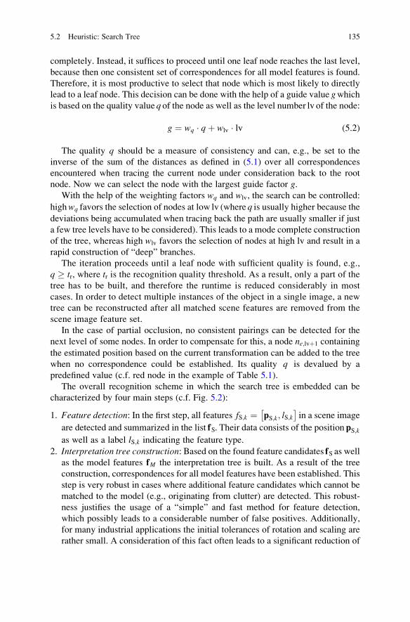
completely. Instead, it suffices to proceed until one leaf node reaches the last level,

because then one consistent set of correspondences for all model features is found.

Therefore, it is most productive to select that node which is most likely to directly

lead to a leaf node. This decision can be done with the help of a guide value gwhichis based on the quality value q of the node as well as the level number lv of the node:

g ¼ wq � qþ wlv � lv (5.2)

The quality q should be a measure of consistency and can, e.g., be set to the

inverse of the sum of the distances as defined in (5.1) over all correspondences

encountered when tracing the current node under consideration back to the root

node. Now we can select the node with the largest guide factor g.With the help of the weighting factors wq and wlv, the search can be controlled:

highwq favors the selection of nodes at low lv (where q is usually higher because thedeviations being accumulated when tracing back the path are usually smaller if just

a few tree levels have to be considered). This leads to a mode complete construction

of the tree, whereas high wlv favors the selection of nodes at high lv and result in a

rapid construction of “deep” branches.

The iteration proceeds until a leaf node with sufficient quality is found, e.g.,

q � tr, where tr is the recognition quality threshold. As a result, only a part of the

tree has to be built, and therefore the runtime is reduced considerably in most

cases. In order to detect multiple instances of the object in a single image, a new

tree can be reconstructed after all matched scene features are removed from the

scene image feature set.

In the case of partial occlusion, no consistent pairings can be detected for the

next level of some nodes. In order to compensate for this, a node ne;lvþ1 containingthe estimated position based on the current transformation can be added to the tree

when no correspondence could be established. Its quality q is devalued by a

predefined value (c.f. red node in the example of Table 5.1).

The overall recognition scheme in which the search tree is embedded can be

characterized by four main steps (c.f. Fig. 5.2):

1. Feature detection: In the first step, all features fS;k ¼ pS;k; lS;k� �

in a scene image

are detected and summarized in the list fS. Their data consists of the position pS;kas well as a label lS;k indicating the feature type.

2. Interpretation tree construction: Based on the found feature candidates fS as wellas the model features fM the interpretation tree is built. As a result of the tree

construction, correspondences for all model features have been established. This

step is very robust in cases where additional feature candidates which cannot be

matched to the model (e.g., originating from clutter) are detected. This robust-

ness justifies the usage of a “simple” and fast method for feature detection,

which possibly leads to a considerable number of false positives. Additionally,

for many industrial applications the initial tolerances of rotation and scaling are

rather small. A consideration of this fact often leads to a significant reduction of


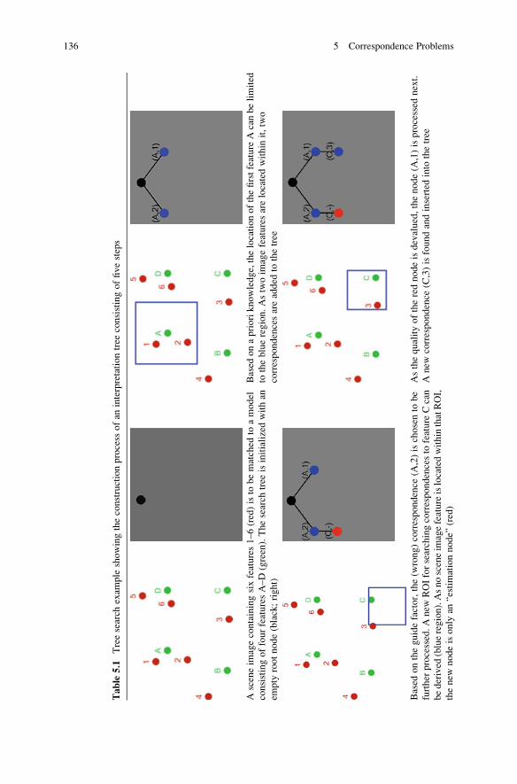
Table

5.1

Treesearch

exam

ple

showingtheconstructionprocess

ofan

interpretationtree

consistingoffivesteps

Asceneim

agecontainingsixfeatures1–6(red)isto

bematched

toamodel

consistingoffourfeaturesA–D(green).Thesearch

tree

isinitializedwithan

empty

rootnode(black;right)

Based

onaprioriknowledge,thelocationofthefirstfeature

Acanbelimited

totheblueregion.Astwoim

agefeaturesarelocatedwithin

it,two

correspondencesareadded

tothetree

Based

ontheguidefactor,the(w

rong)correspondence

(A,2)ischosento

be

further

processed.Anew

ROIforsearchingcorrespondencesto

feature

Ccan

bederived

(blueregion).Asnosceneim

agefeatureislocatedwithinthatROI,

thenew

nodeisonly

an“estim

ationnode”

(red)

Asthequalityoftherednodeisdevalued,thenode(A

,1)isprocessed

next.

Anew

correspondence

(C,3)isfoundandinserted

into

thetree


Inthenextstep,node(C,3)isexpanded.Thesize

ofthesearch

region(blue)

canbereducedas

thepositionestimatebecomes

more

accurate.Two

correspondencesarefoundandadded

tothetree

Inthenextstep,theROIsize

canbereducedfurther,andacorrespondence

for

lastmodelfeature

ofthesearch

order

(B)isfound.Hence,acompletesolution

isavailable(green

node).Anaccuratepositionestimationbased

onthefound

correspondencesisalso

possible

From

Treiber

[23],withkindpermissionfrom

Springer

Science

andBusinessMedia


possible correspondences, too, because the search areas (blue regions in

Table 5.1) can be kept rather small.

3. Transformation estimation: The parameters t of the transformation T (e.g., the

four parameters translation tx; ty� �

, rotation θ , and scale s of a similarity

transform) are estimated with the help of the found correspondences.

4. Inspection (optional): Based on the detected features, it is often easy to decide

whether the part has been manufactured with sufficient quality. For example, it

could be checked whether the position of a drilling, which can easily be

represented by a specific feature, is within its tolerances.

Pseudocode

function detectObjectPosInterpretationTree (in Image I, in

ordered list fM of model features fM;i ¼ pM;i; lM;i

� �, in distance

threshold td, in recognition threshold tr, out object positionlist p�)

// step 1: feature detection

detect all feature candidates fS;k ¼ pS;k; lS;k� �

in scene image I

and arrange them in list fSwhile fS is not empty do // loop for multiple obj. detection

init of tree st with empty root node nroot; set its qualityvalue qroot to maximum qualitybFound FALSE

// step 2: search tree construction (loop for detection ofa single object instance)lv 0

Model

Matching

Feature extraction

Transformation estimation

Inspection

Fig. 5.2 Illustrating the proceeding of object detection with interpretation trees for a stamped

sheet as a typical example for an industrial part (From Treiber [23], with kind permission from

Springer Science and Business Media)


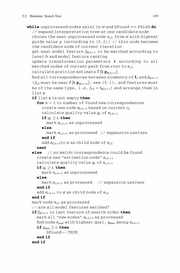
while unprocessed nodes exist in st and bFound ¼¼ FALSE do// expand interpretation tree at one candidate nodechoose the next unprocessed node ni;lv from st with highestguide value g (according to (5.2)) // this node becomesthe candidate node of current iterationget next model feature fM;lvþ1 to be matched according tolevel lv and model feature rankingupdate transformation parameters t according to allmatched nodes of current path from root to ni;lvcalculate position estimate T t; pM;lvþ1

� �

find all correspondences between elements of fS and fM;lvþ1( fS;k must be near T t; pM;lvþ1

� �, see (5.1), and features must

be of the same type, i.e. lS;k ¼ lM;lvþ1) and arrange them inlist cif list c is not empty then

for k ¼ 1 to number of found new correspondencescreate new node nk;lvþ1 based on current ckcalculate quality value qk of nk;lvþ1if qk � tr then

mark nk;lvþ1 as unprocessedelse

mark nk;lvþ1 as processed // expansion uselessend ifadd nk;lvþ1to st as child node of ni;lv

nextelse // no match/correspondence could be found

create new “estimation node” ne;lvþ1calculate quality value qe of ne;lvþ1if qe � tr then

mark ne;lvþ1 as unprocessedelse

mark ne;lvþ1 as processed // expansion uselessend ifadd ne;lvþ1 to st as child node of ni;lv

end ifmark node ni;lv as processed// are all model features matched?if fM;lvþ1 is last feature of search order then

mark all “new nodes” nk;lvþ1 as processedfind node ngoal with highest qual. qmax among nk;lvþ1if qmax � tr then

bFound TRUEend if

end if


lv lvþ 1

end whileif bFound ¼ TRUE then

// step 3: transformation estimationcollect all correspondences by tracking the tree backfrom ngoal to nrootestimate the parameters t� of T by performing minimiza-tion of position deviations for all correspondencesadd t� to position list p�

remove all matched features from list fSelse

return // no more object instance could be foundend if

end while

5.2.3 Example

An example of recognizing industrial parts like stamped sheets is presented in

Table 5.2. The objects are recognized by utilizing different parts of their contour as

features to be matched. Please observe that correct correspondences are found even

in scenes with a significant amount of clutter.

Please note that the method is much more robust with respect to clutter (when

trying to expand the tree at a node that is based on a correspondence originating

from clutter, there is no consistent correspondence very quickly) compared to

occlusion (disadvantageous trees are possible especially if the first correspondences

to be evaluated don’t exist because of occlusion).

To sum it up, interpretation trees are well suited for industrial applications,

because the method is relatively fast, an additional inspection task fits well to the

method, and we can concentrate on detecting characteristic details of the objects.

On the other hand, the rigid object model is prohibitive for objects with consider-

able variations in shape.

5.3 Iterative Closest Point (ICP)

5.3.1 Standard Scheme

Another algorithmic concept which deals with the task of the registration of a data

point set PD ¼ pD;i� �

; 1 � i � ND to a set of model points PM ¼ pM;j

n o; 1 � j

� NM is the Iterative Closest Point algorithm (ICP). As the method provides a

framework, it can be adapted to and used in various applications. Both the


registration of 2D and 3D point sets is possible with ICP. The basic form of the

algorithm was initially proposed in [2].

The goal of registration is to find a common coordinate reference frame for both

point sets and hence identify a transformation between the two sets. Consequently,

the task is twofold:

• Establish the correct correspondences between the elements ofPD andPM. In this

context, this means that for each element i of the data point set, it should be

Table 5.2 Giving more detailed information about the detection and position measurement of

stamped sheets, which are a typical example of industrial parts

Scene image containing several stamped sheets.

Due to specular reflections, the brightness of the

planar surface is not uniform. One object is

completely visible and shown in the upper-left

area

View of all detected features (marked red). The

object model consists of the holes and some

corners, which are detected independently.

Several additional features are detected due to

clutter

Interpretation tree: found correspondences are

marked green; estimated correspondences are

marked red. Due to clutter, many

correspondences are found for the first feature of

the search order. However, the search is very

efficient, e.g., the solution is almost unique after

the third level

Matched features of the final solution of the tree

(marked green). All correspondences are

established correctly. An inspection step, e.g.,

for the holes, could follow

From Treiber [23], with kind permission from Springer Science and Business Media

5.3 Iterative Closest Point (ICP) 141

matched to the “closest” model point j, where the function j ¼ ϕðiÞ describes themapping.

• Estimate the parameters t of a transformation T, which describes the relationshipbetween the two coordinate frames.

Now let’s assume that some correspondences have been found already (i.e., a

first estimate ofϕ is known). This is a reasonable assumption for some applications,

e.g., initial correspondences could be estimated by matching descriptors. Then, a

typical way to estimate the parameter vector t is to minimize an energy function

E t;ϕð Þbeing composed of the sum of squared distances between the positions of the

transformed data points pD;i and the positions of their corresponding model points

pM;ϕðiÞ:

t� ¼ argmint

E t;ϕð Þ½ � ¼ argmint

XND

i¼1pM;ϕðiÞ � T t; pD;i

� ��2

" #(5.3)

As ϕ has to be estimated in the optimization process, too, the energy E t;ϕð Þ canbe reformulated as

E tð Þ ¼XND

i¼1minj

pM;j � T t; pD;i� �� 2 (5.4)

where the min-operator selects that model point being located closest to a

specific data point pD;i . Observe that the min-operator prohibits a straightforward

closed form solution of (5.4). Therefore, the optimization of (5.4) is done itera-

tively, where two steps are performed in alternation. Starting at an initial transfor-

mation estimation t0, the following two steps are executed iteratively:

1. Correspondence estimation: While fixing the current transformation tk, for eachdata point, find the model point, which is located closest to the position of this

data point after application of the current transformation estimation tk , i.e., foreach data point pD;i apply

ϕkðiÞ ¼ argminj2PM

pM;j � T tk; pD;i� �� 2 (5.5)

2. Transformation estimation: Now, as ϕk is known, we can solve the following

least mean squares problem in closed form, e.g., for linear transformations by

applying linear regression:

tkþ1 ¼ argmint

XND

i¼1pM;ϕkðiÞ � T tk; pD;i

� ��2

(5.6)

The convergence criterion is quite obvious: if the correspondences ϕk don’t

change any more compared to the previous iteration, we will end up with an


unchanged transformation estimate, too. Consequently, the method has converged.

An overview of the proceeding is given in the flowchart of Fig. 5.3.

The iterative nature implies that the ICP algorithm performs a local search around

the current estimate. However, typically we cannot assume that E tð Þ is convex.

Therefore, we are in danger of being “trapped” in a local minimum if the initial

estimate t0 is located too far from the global optimum. For that reason ICP is basically

just a refinement scheme, i.e., it requires some reasonably good initial estimate, e.g.,

by evaluating descriptor information. In some cases, the method can start without any

prior knowledge by taking the identity transform as starting point. However, this only

works if the two point sets already are aligned sufficiently well at start.

A possible way out would be to perform the ICP algorithm multiple times with

different initial transformations and select that solution yielding the lowest energy

at convergence. However, this proceeding increases the runtime of the algorithm

considerably and still we cannot be sure that one of the initial estimates is suffi-

ciently close to the optimum.

5.3.2 Example: Robust Registration

In order to enlarge the limited convergence area of the standard ICP algorithm and

thereby increase its robustness, many modifications have been proposed. Here we

will present the work of Fitzgibbon (see [7]) in more detail. Fitzgibbon proposed to

replace the Euclidean-based distance measure in (5.4) by a more robust estimate.

However, the introduction of a robust distance measure involves difficulties when

trying to estimate the transformation parameters in step 2 of ICP in closed form.

Therefore, in [7] it is suggested to utilize a general purpose regression scheme like

the Levenberg-Marquardt algorithm [15] instead. Consequently, we take a closer

look how the Levenberg-Marquardt algorithm can be applied to this specific

problem.

A first step to increase the robustness of ICP is to allow for unmatched points.

Consider the situation where a pointpD;i in the data point set is present due to clutter

and actually doesn’t have a correspondence in the model point set. This situation

occurs quite often in practice. However, standard ICP as presented above always

SFind all clos-est points,based on t k

Re-estimatet k+1 , based oncurrent corresp.

Corresp. un-changed ?

E

no

yes

Fig. 5.3 Flowchart of the ICP proceeding


matches every data point to some model point. This could lead to a large distance

for pD;i, and therefore, the (wrong) correspondence introduces a large error in (5.4).

This situation can be alleviated by introducing weights wi 2 0; 1f g in step 2 of

ICP. A weight wi is set to zero if no correspondence could be found for pD;i, e.g.,

when its transformed position is too far away from any model point. If a correspon-

dence was found, wi is set to 1.

The main contribution Fitzgibbon [7] in order to increase robustness, however, is

to replace the Euclidean-based distance pM;ϕðiÞ � T t; pD;i� ��

��2

(abbreviated as xk k2

in the following) by a more robust measure ε xð Þ2, such as the so-called Huber kernel:

ε xð Þ2 ¼ xk k2 xk k < σ2σ xk k � σ2 otherwise

(5.7)

Compared to the Euclidean distance measure, the Huber kernel takes smaller

values for large distances, i.e., when xk k > σ (see Fig. 5.4, with σ ¼ 3). As a

consequence, the influence of large distances in (5.6) is reduced.

As can be seen in Fig. 5.5, the area of convergence can be increased considerably

through the usage of the Huber kernel compared to standard ICP (compare the green

to the light blue curve). The left part of the figure depicts an application where two 2D

curves (black and blue dots) are to be aligned. For the tests, the lower right “C” has

been rotated synthetically prior to matching it to the upper-left “C.” In the diagram at

the right, the x-axis denotes the rotation difference between the initial transformation

estimation and the actual rotation between the two point sets in degrees, and the

y-axis plots some error measure after the algorithm has converged. As clearly can be

seen, the introduction of the Huber kernel allows for far larger errors in the initial

0

20

40

60

80

100

120

0

0.5 1

1.5 2

2.5 3

3.5 4

4.5 5

5.5 6

6.5 7

7.5 8

8.5 9

9.5 10

Euclid

Huber

Fig. 5.4 Comparison of the Euclidean distance measure with the Huber kernel: the x-axis denotesthe distance xk k, and σ is set to 3


rotation estimate as it leads to smaller total errors after convergence for a larger

rotation deviation range.

The problem which is involved with the usage of the Huber kernel is that now the

solution of the transformation estimation (step 2 of ICP) in closed form is compli-

cated by the case-by-case analysis in (5.7). As a consequence, the minimization

problem in the transformation step has to be solved numerically. Here we can make

use of the fact that the total error measure is a sum of squared contributions Ei tð Þfrom the individual correspondences, which can be stacked into a vector e:

E tð Þ ¼XND

i¼1Ei tð Þ2 ¼ eT � e

with Ei tð Þ ¼ ffiffiffiffiffiwip �min

jε pM;j � T t; pD;i

� �� (5.8)

Through approximating (5.8) by a Taylor expansion around the current transfor-

mation estimate tk , applying a Gauss-Newton approximation (approximate the

second order derivatives with the Jacobi matrix) and making use of the vector e,we can write

E tk þ Δ� � � eT � eþ 2 � Δ � JT � eþ ΔT � JT � J � Δ (5.9)

where theΔ vector denotes the transformation parameter differences with respect to

tk and Jacobi-Matrix J contains the partial first-order derivatives of the Ei tð Þ. Itconsists of ND L elements (L is the number of transformation parameters), which

can be calculated via Jil ¼ @Ei tk

� �@tl= .

Fig. 5.5 Illustrating the improved area of convergence, when the robust Huber kernel is used (as

far as rotation deviations are concerned) (Reprinted from Fitzgibbon [7], with permission from

Elsevier)


An iterative optimization scheme can now estimate theΔ vector and then update

the current transformation estimate accordingly: tkþ1 ¼ tk þ Δ.Fitzgibbon suggested to use the Levenberg-Marquardt optimization algorithm,

which combines updates according to Gauss-Newton as well as gradient descent

(see Chap. 2). With Gauss-Newton,Δ is set toΔ ¼ � JT � J� ��1 � J � e, whereas withgradient descent, we have Δ ¼ �λ�1 � JT � e . Overall, the update of LM can be

written as

Δ ¼ � JT � Jþ λ � I� ��1 � J � etkþ1 ¼ tk þ Δ

(5.10)

with I being the identity matrix. At each iteration of the second step of the modified

ICP algorithm, one update step according to LM (see (5.10)) is performed. In order

for LM algorithms to perform well, the parameter λ , which controls the relative

weight of Gauss-Newton and gradient descent, has to be chosen sufficiently well. In

early steps, λ is chosen large, such that the gradient descent dominates. Thereby, the

method takes small steps, where we can be quite sure that the error function is

actually reduced. As the iteration proceeds, λ is reduced successively, which gives

more emphasis to Gauss-Newton, because it can be assumed that the Taylor

approximation used in Gauss-Newton has little error near the optimum, and,

therefore, we can make use of the fast convergence of Gauss-Newton.

One question still to be answered is how to calculate the elements Jil of the Jacobimatrix, which involve taking derivatives of Ei tð Þ. A numerical approach is to take

finite differences, i.e., at the current transformation estimate tk, we calculate Ei tk

� �,

modify tk by an arbitrarily chosen small amount δtk, calculateEi tk þ δtk

� �, and take

the difference toEi tk

� �. The author of [7] pointed out the importance of reestimating

the correspondences when moving from tk to tk þ δtk. Hence, each Jil ¼ @Ei tk

� �@tl=

can be calculated as follows:

1. calculateEi tk

� �, based on the current closest point of the model point set pM;ϕkðiÞ,

which was determined during step one of ICP.

2. Choose a small δtk (where only the l-th component is different from zero) and

reestimate the closest model point (yielding p0M;ϕkðiÞ ), based on the modified

transformation tk þ δtk. Please note that this correspondence could change as wemove from tk to tk þ δtk.

3. calculate Ei tk þ δtk

� �, based on the (potentially) updated p0M;ϕkðiÞ

4. set Jil ¼ Ei tk

� �� Ei tk þ δtk

� �� δtk

��

The usage of the robust measure ε xð Þ in conjunction with the LM algorithm leads

to better performance but at the same time to increased execution time, as the

calculation of the derivatives needs extra time. Therefore, Fitzgibbon suggested a

speedup of the algorithm through the usage of a so-called distance transform, which


http://dx.doi.org/10.1007/978-1-4471-5283-5_2

exploits the fact that the penalties of transformed data points, compared to their

closest model points depend only on the model point set for a given data point

position. Consequently, they can be calculated prior to the ICP iterations and be

reused for different data points pD;i and transformations t (see [7] for details).

Figure 5.6 illustrates the superior performance of the modified algorithm as

suggested in [7] compared to standard ICP for 3D point sets. The point sets

which are to be aligned consist of points located on the surface of a bunny. The

standard ICP method, whose result is displayed in the right part of the top row,

clearly shows considerable deformations between model and transformed data

point sets. Compared to this, the two sets are aligned much better when the

algorithm of [7] is used.

Fig. 5.6 Showing the performance gain of the algorithm of [7] (bottom), compared to standard

ICP (top). In this application, two sets of 3D points located on the surface of a bunny (blue and redpoints) are to be aligned (Reprinted from Fitzgibbon [7], with permission from Elsevier)


Pseudocode

function robustICPRegistration (in data point set PD ¼ pD;i� �

,

in model point set PM ¼ pM;j

n o, in initial transformation

estimate t0 , in maximum correspondence distance dmax , outcorrespondences ϕ�, out final transformation estimate t�

k 0// main loop of ICPrepeat

// step 1: find closest point for each data pointfor i ¼ 1 to ND

di;min max_floatfor j ¼ 1 to NM

dij ¼ pM;j � T tk; pD;i� ��

// do we have a new closest point candidate?if dij < di;min then

di;min dijϕkðiÞ j

end ifif dij > dmax then

wi 0 // max. distance exceeded -> no corresp.else

wi 1 // distance limit okend if

nextnext// step 2: update transformation parameters// calculate Jacobi matrixfor i ¼ 1 to ND

calculate Ei tk

� �according to (5.8)

for l ¼ 1 to L // L: number of transformation params

set δtk ¼ 0; 0; . . . ; δ; 0; . . . ; 0½ � // only lth elem 6¼ 0

re-estimate correspondence ϕkðiÞ0calculate Ei t

k þ δtk� �

based on ϕkðiÞ0 according to (5.8)

set Jil ¼ Ei tk

� �� Ei tk þ δtk

� �� δtk

��

nextnextupdate λcalculate Δ and update transformation estimate tkþ1

according to (5.10)k k þ 1

until convergence, e.g. ϕkþ1 ¼ ϕk or E tkþ1� �� E tk

� �� E tkþ1� ��

þE tk� �Þ � δ

t� tk

ϕ� ϕk


5.4 Random Sample Consensus (RANSAC)

Considering the task of image registration, where we have to align two (or more)

images which at least partly overlap, we can detect a set of interest points in both

images (P1 ¼ p1;m ;m 2 1; . . . ;M½ �� and P2 ¼ p2;n ; n 2 1; . . . ;N½ ��

). We could

then use the ICP algorithm which performs an iterative refinement of the

correspondences as well as the transformation estimate between the two point

sets. However, in order to work properly, the ICP algorithm needs a sufficiently

well chosen initial estimate of the transformation, which allows the algorithm to

converge to the desired optimum.

Additional information can be obtained if we derive descriptors from a local

image patch around each interest point, e.g., by calculating SIFT descriptors

[14]. This adds up to two sets of descriptors D1 ¼ d1;m� �

and D2 ¼ d2;n� �

. As

already mentioned, we can make use of this descriptor information in order to get a

sufficiently “good” initial estimate of the aligning transform and then apply the ICP

algorithm. A straightforward approach would be:

1. Detect the set of interest points P1 and P2 in both images, e.g., by detecting

corner-like points with the Harris detector [8].

2. Derive a descriptor from the image patch around each interest point yielding the

descriptor sets D1 and D2, e.g., SIFT [14].

3. Establish correspondences n ¼ ϕðmÞ between the elements of D1 and the

elements of D2 yielding the correspondence set Φ . A correspondence is

established if fsim d1;m; d2;n� � � tsim, where fsim is some measure estimating the

similarity between the two descriptors (e.g., the inverse of the Earth Mover’s

Distance or χ2 distance; see e.g., [18]) and tsim a similarity threshold.

4. Estimate the parameters t of the transformation T between the two images, e.g.,

by a least squares approach, which minimizes the sum of the distances between

p1;m and T t; p2;ϕðmÞ�

.

5. Refine ϕ and t with the ICP algorithm.

The problem with this proceeding is that all correspondences are taken into

account when estimating the transform parameters. Wrong correspondence

estimates usually introduce gross errors and therefore can seriously spoil the

transformation estimation. Averaging methods like least squares (which is optimal

for Gaussian-distributed errors) assume that the maximum error between the

“observation” (here: p1;m ) and the “model” (here: T t; p2;ϕðmÞ�

) is related to the

size of the data set, and, therefore, averaging can successfully smooth large errors

(this assumption is termed smoothness assumption in literature).

However, this doesn’t have to be true here: a few wrongly estimated

correspondences lead to some large error terms being far from the distribution of

5.4 Random Sample Consensus (RANSAC) 149

the remaining errors. This is where RANSAC (Random Sample Consensus) [6]comes into play. The RANSAC proceeding is more a paradigm than a specific

algorithm. It can also be used for the problem of image registration, and, therefore,

we will present RANSAC in this context.

Fisher et al. [6] distinguish between two sources of error:

• Measurement error: This type of error is introduced when measuring the data,

e.g., when the measured position of an interest point deviates a bit from its “true”

position, e.g., due to sensor noise. Many sources of noise or other perturbations

are normally distributed, and, therefore, usually the smoothness assumption

holds for this type of errors.

• Classification error: Many algorithms feature a hard decision, which in our case

is the assignment of correspondences. Errors like the estimation of a wrong

correspondence (which can occur if many descriptors are very similar) can

introduce large deviations and are in general not related to the data set size.

Therefore, the smoothness assumption does not hold for this type of error.

As a consequence, we need a method which is robust in the sense that it features

a mechanism which automatically ignores gross errors and not just tries to averagethem out. The RANSAC approach exactly aims at achieving this. It is designed

such that it tolerates as many outliers as possible. The basic proceeding after

estimating the correspondences (step 3 of the procedure outlined above) is as

follows (see also the flowchart of Fig. 5.7):

4. Random selection: Randomly select a subset of the data (here: a subsetΦR of all

found correspondences). The size of this subset should be as small as possible.

For example, for affine transformations in 2D, only three points are necessary in

order to uniquely determine the six transformation parameters. Therefore, only

three correspondences should be chosen at this step.

S

E

yes

no

Interest pointand descriptor

calculation

Detect indi-vidual corre-spondences

Generatehypothesis t

Consensus setlarge enough ?

Add all con-sistent corre-spondences toconsensus set

Re-estimatet∗

Fig. 5.7 Flowchart of the RANSAC proceeding


5. Model instantiation: Based on this subset, a first instance of the model should be

derived. In our case, the transformation parameters t can be calculated

completely based on the selected correspondences.

6. Consistency check: Based on the initial model estimation (here: transformation

estimation t), we can check all data (correspondences) whether they are consis-

tent with this initial estimation. This mean here that the transformed position T

t; p2;ϕðmÞ�

has to be sufficiently close to p1;m: if T t; p2;ϕðmÞ�

� p1;m

�� ε, the

correspondence n ¼ ϕðmÞ is added to the subset ΦR (also called consensus set).7. Termination check: If the size of the enlarged consensus set is above some

threshold tsize, it can be assumed that only inliers were chosen as initial consensus

set, and, therefore, the transformation estimate is broadly supported by the data.

Therefore, the final transformation parameters t� are reestimated based on the

enlarged consensus set. If tsize is not reached, the process is restarted at step

4 until the maximum number of trials Nmax is reached.

Observe that RANSAC fundamentally differs from the schemes up to now.

Whereas methods like ICP, for example, try to optimize a current solution in

some form, RANSAC is essentially a hypothesis testing scheme: basically, step

4 formulates a hypothesis about the solution, which is then tested for consistency

with the rest of the data.

The RANSAC proceeding contains three parameters, (ε, tsize , and Nmax), whose

values have to be chosen properly in advance. As far as ε is concerned, it is often

determined empirically. To this end, a scenario with known correspondences can be

created. Next, the data set is artificially corrupted by noise. Based on the errors which

were introduced, the transformation estimation is affected more or less seriously. As

we also know the “ground truth,” it is possible to quantify the error introduced by the

perturbation. Based on this quantification it should be possible to choose ε such that itseparates correct from wrong correspondence estimates sufficiently well.

In contrast to that, the parameters tsize andNmax can be calculated in closed form.

They are mainly influenced by the proportion of outliers as well as the desired

probability that at least one random pick exclusively contains inliers. Details can be

found in [6].

An illustration of the performance of a RANSAC-based correspondence/transfor-

mation estimation can be seen in Fig. 5.8. Here, two images of the same scene taken

from different viewpoints can be seen in (a) and (b). The yellow points of (c) and

(d) indicate the detected interest points. The initial estimation of correspondences is

visualized by yellow lines in (e) and (f). Correspondences were estimated based on

simple normalized cross correlations of the intensity values of a patch around each

interest point. Clearly, these initial correspondences contain a significant proportion

of outliers. The consensus set after applying the RANSAC procedure can be seen in

(g) and (h). Their visual appearance indicates that all outliers were ignored by the

procedure.


Fig. 5.8 Illustrating the performance of a RANSAC-based correspondence estimator. See text for

details (From Hartley and Zisserman [9], with kind permission)


Pseudocode

function robustRANSACImageRegistration (in image I1 , inimage I2, in algorithm parameters tsim, ε, tsize, and Nmax, outconsensus set of consistent correspondences ΦR , out finaltransformation estimate t�

// interest point and descriptor calculation

detect set of interest pointsP1 ¼ p1;m;m 2 1; . . . ;M½ �� in image I1

, e.g. with Harris detector

detect set of interest pointsP2 ¼ p2;n; n 2 1; . . . ;N½ �� in image I2,

e.g. with Harris detectorderive a descriptor d1;m for each interest point p1;m from the

patch of image I1 around it, e.g. SIFT descriptorderive a descriptor d2;n for each interest point p2;n from the

patch of image I2 around it, e.g. SIFT descriptor

// correspondence detectionΦ fgfor n ¼ 1 to N // loops for every possible descr. combination

for m ¼ 1 to M

if fsim d1;m; d2;n� � � tsim then

add n ¼ ϕðmÞ to the correspondence set: Φ Φ [ ϕf gend if

nextnext

// robust RANSAC transformation estimationk 0repeat

randomly select a subset ΦR with minimum size out of Φ// step 1

estimate t based on ΦR // step 2// enlarge ΦR, if additional correspondences are consis-

tent with t (step 3)for i ¼ 1 to Φj j // loop for all “remaining” correspondences

if ϕi=2ΦR ^ T t; p2;φiðmÞ�

� p1;m

�� ε then

add n ¼ ϕðmÞ to the consensus set: ΦR ΦR [ ϕf gend if

nextk k þ 1

until ΦRj j � tsize or k ¼ Nmax // step 4re-estimate t� based on the enlarged consensus set ΦR


In the meantime, quite numerous extensions/modifications in order to improve

performance have been proposed (see e.g., [3] for a quick systematic overview).

The authors of [3] classify the modifications according to the aspect of RANSAC

they seek to improve:

• Accuracy: These modifications aim at optimizing the correctness of the

estimated parameters t� of the aligning transform. One possibility is to reestimate

t� by taking all consistent correspondences into account, as already mentioned.

Apart from that, we can modify the way a hypothesis is evaluated. Standard

RANSAC simply counts the number of inliers in step 7 of the proceeding

outlined above. However, such a hard decision does not take the error

distributions of inliers and outliers into account. A better way is to assign a

cost to each tested datum which varies more smoothly with respect to the

consistency with the hypothesis to be tested and then to sum up all these costs.

• Speed: Variations of this category intend to optimize the runtime of the algo-

rithm. One way is to consider similarity scores of individual correspondences

(e.g., descriptor similarity), if available. These similarity scores allow for a

ranking of the correspondences. We can try to make use of this information by

choosing top-ranked data with high probability during the random selection

process of step 4. This accounts for the fact that correspondences being based

on descriptors with high degree of similarity are more likely to be correct that

those with low descriptor similarity. As a result, on average the method needs

less iterations until convergence is achieved.

• Robustness: As the RANSAC method needs some parameters (ε, tsize, and Nmax),

which affect its performance, care is required when choosing their values. To

this end, there have been several suggestions to tune their parameters, either

based on a priori considerations or depending on the nature of the data at hand

(see [3] for details).

5.5 Spectral Methods

5.5.1 Spectral Graph Matching

The method proposed by Leordeanu and Herbert [13] takes an alternative approach

in order to make the correspondence estimation more robust. Here, the problem is

represented by a properly constructed graph, which is built in a first step. Next, the

solution can be obtained by an adequate examination of the graph through utilizing

its so-called spectral properties (see below). This method is also an example of the

usage of relaxation methods for discrete optimization problems.

In [13] two issues are considered during correspondence estimation:

1. Individual correspondence affinity: This term measures the confidence that two

points p1;m and p2;n (which are elements of two different point sets

P1 ¼ p1;m;m 2 1; . . . ;M½ �� andP2 ¼ p2;n; n 2 1; . . . ;N½ ��

) form a correspon-

dence if we just consider the properties of the points themselves, i.e., without


taking their relation to other points into account. This can be done by calculating

a descriptor-like SIFT [14] for each point (yielding d1;m and d2;n ) and then

measuring the individual affinity through the similarity betweend1;m andd2;n, forexample. If a potential correspondence is very unlikely, e.g., becaused1;m differs

much fromd2;n, this correspondence is not accepted, i.e., no node is created in thegraph.

2. Pairwise affinity: Here, a pair of possible correspondences is considered. Imagine

that we want to evaluate how consistent it would be if we matchedp1;m1top2;n1 (in

the following denoted as possible correspondence a) and p1;m2to p2;n2 (possible

correspondence b). A measure of consistency between a and b could be based on

the similarity of the distance between p1;m1and p1;m2

to the distance between p2;n1and p2;n2 . If the distances are similar, it is likely that the relationship between the

points of both correspondences can be expressed by the same transformation.

Please note that this measure is only suitable for distance-preserving

transformations like the Euclidean transformation considering translation and

rotation. This metric doesn’t work any longer when we also want to consider a

significant amount of scaling, for example.

A measure m a; bð Þ for the distance similarity used in [13] is given in the

following, where g i; jð Þ denotes some distance measure between i and j, whereasthe parameter σd controls the sensitivity of the metric with respect to discrepancies

in the distances. For small σd,m a; bð Þ declines rapidly when the difference betweenthe two distances increases.

m a; bð Þ ¼ 4:5� g m1;m2ð Þ�g n1;n2ð Þ½ �22σd2

if g m1;m2ð Þ � g n1; n2ð Þj j < 3σd0 otherwise

((5.11)

Based on these two types of affinity, the correspondence problem can be

represented by an appropriately constructed graph. Each node na of the graph

utilized in [13] correlates to a possible correspondence a between a point p1;m of the

first and a point p2;n of the second point set. A weight depending on the individual

correspondence affinity can be attributed to each node. For example, the degree of

similarity between the two descriptors around the points represented by the poten-

tial correspondence can be taken as a weight, which can be set to some similarity

measure fsim d1;m; d2;n� �

, e.g., the inverse of the Earth Mover’s Distance or χ2

distance (see e.g. [18]) being based on the descriptors derived for each point.

Furthermore, two nodes na and nb are linked by an edge eab if their pairwise affinitymeasurem a; bð Þ is larger than zero. The weight associated with eab can be set equalto m a; bð Þ.

The key observation of Leordeanu et al. [13] is that potential correspondences,

which are consistent to a common transformation, tend to form a large cluster in the

graph, where the nodes are strongly connected to each other (connection strength is

indicated by the pairwise affinities as defined above). Outliers, in turn, tend to form

5.5 Spectral Methods 155

“isolated” connections. As a consequence, the task here is to find the largest

strongly connected cluster of the graph.

This can be done by representing the graph through its so-called adjacency

matrix M, which incorporates the weights of the graph nodes and edges:

• The diagonal elementsm a; að Þ represent the individual correspondence affinities,i.e., the weights associated to the nodes of the graph (e.g., the descriptor

similarities). Observe that usually many possible correspondences can be

excluded from the solution search, because their individual similarity is very

low. In that case we can reduce the size of M by simply not considering those

correspondences when M is constructed, i.e., by omitting row/column a. As aconsequence, M stays rather small (of dimensionality NC NC , where NC

denotes the number of combinations between two descriptors of different sets

with a similarity above some threshold tsim ). This accelerates the subsequent

optimization considerably. If no individual correspondence affinity measure is

available, the m a; að Þ can be set to zero. Of course, the size of M cannot be

reduced in that case (which means thatM is aM � N M � N–matrix in that case).

• The off-diagonal elements m a; bð Þ represent the pairwise affinities, which can be

calculated, e.g., via (5.11). Generally it can be assumed thatm a; bð Þ ¼ m b; að Þ, andtherefore, M is symmetric. Observe that m a; bð Þ is zero if the distance difference

between pairs of potential correspondences is large. This should be the case for

many pairs, so in general M is a sparse matrix. As each weight m a; bð Þ (and the

m a; að Þ, too) is nonnegative,M is a nonnegative matrix of dimensionalityNC NC.

How can we utilize M in order to get a solution to our problem? The goal is to

find the cluster in the graph with maximum cumulative weights. To this end, we can

introduce an indicator vector x consisting ofNC elements, which indicates which of

the possible correspondences are actually selected as (correct) correspondences.

The element xðaÞ is equal to 1 if a represents a correct correspondence and zero

otherwise. Then the sum S of those weights associated with the chosen

correspondences can be calculated by S ¼ xT �M � x. As we want to find the largestcluster in the graph where many correspondences are tightly connected, we seek for

the indicator vector yielding the maximum value of S. Consequently, the

correspondences to be found are specified by:

x� ¼ argmaxx

xT �M � x� �(5.12)

Please note that usually the value of one element of x influences some others,

because the correspondences obey some constraints, depending on the application.

A frequently used constraint is that a point in one set can be matched to at most one

point of the other set. Consequently, if a represents the possible correspondence

between p1;m1and p2;n1 and xðaÞ ¼ 1, then all other elements of x related to p1;m1

or

p2;n1 have to be equal to zero. Otherwise the solution of (5.12) would be trivial

because of the nonnegativity of M , the highest score would be achieved if we


consider all possible correspondences, i.e., all entries of x are set to one. Hence, wehave two constraints to be considered in (5.12):

• Matching constraints (as just described)

• The elements of xðaÞ can either be one or zero.

The authors of [13] now suggest a scheme which at first finds a solution by

ignoring both of these constraints and then updates the solution by considering the

constraints again. Ignoring the binary nature of the elements of the indicator vector

(only two values are possible: one and zero) leads to relaxation, as now each

element can take continuous values. In this case, we can set the L2-norm of x

equal to one without influencing the solution, i.e., xT � x ¼ 1.

Without constraints, (5.12) is a classical Rayleigh quotient problem (see e.g.,

[22]). This means that if x is set to some eigenvector v ofM, the Rayleigh quotient

will yield the corresponding eigenvalue. As we seek indicator vectors which

maximize (5.12), the solution of the relaxation of (5.12) is the eigenvector belong-

ing to the largest eigenvalue of M. The fact that the largest cluster of the graph is

found with the help of some eigenvalue calculation explains why the method is

termed “spectral.”

This principal eigenvector can be found efficiently with the so-called power

iteration method (see e.g., [22]). Starting from some v0, the method performs the

iterative update

vkþ1 ¼ M � vkM � vkk k (5.13)

The iteration finally converges to the desired principal eigenvector v� . If allelements of v0 are set to nonnegative values, it is ensured that all elements of v� willbe within the interval 0 . . . 1½ �. Remember that all elements of M are nonnegative,

too, and therefore, multiplication with the nonnegative elements of vk always yieldsnonnegative elements again. Moreover, the normalization step of the iteration

ensures that the values are bounded by one. We can interpret a particular value v�

ðaÞ as the confidence that the pairing of points expressed by a indeed is a valid

correspondence, which belongs to the main cluster of the graph.

In order to obtain the final solution, we have to introduce the constraints again.

To this end, in [13] the following iterative greedy proceeding is suggested (see also

flowchart of Fig. 5.9):

1. Acceptance: Select the pairing amax ¼ argmax v�ðaÞ, i.e., choose that element of

v� which has the highest value and add it to the set of estimated correspondences

ΦR . For amax , we can have the highest confidence that it actually is a correct

correspondence.

2. Rejection: Remove amax as well as that elements from v�, where the underlyingpairing is not consistent with amax. For example, if amax contains a point p1;m and

we have to ensure that each point can be part of at most one correspondence, then

we have to remove all elements from v� which contain p1;m, too. After this, we


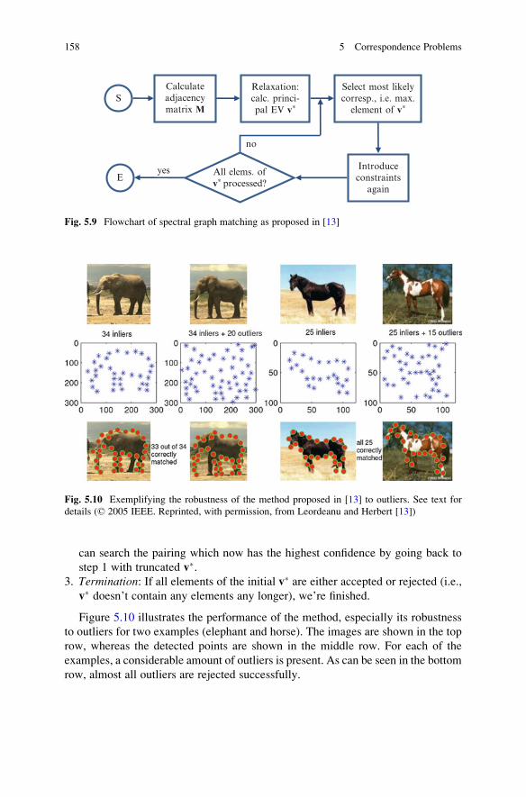
can search the pairing which now has the highest confidence by going back to

step 1 with truncated v�.3. Termination: If all elements of the initial v� are either accepted or rejected (i.e.,

v� doesn’t contain any elements any longer), we’re finished.

Figure 5.10 illustrates the performance of the method, especially its robustness

to outliers for two examples (elephant and horse). The images are shown in the top

row, whereas the detected points are shown in the middle row. For each of the

examples, a considerable amount of outliers is present. As can be seen in the bottom

row, almost all outliers are rejected successfully.

Fig. 5.10 Exemplifying the robustness of the method proposed in [13] to outliers. See text for

details (© 2005 IEEE. Reprinted, with permission, from Leordeanu and Herbert [13])

S

Eyes

no

Calculateadjacencymatrix M

Relaxation:calc. princi-pal EV v∗

Select most likelycorresp., i.e. max.

element of v∗

Introduceconstraints

again

All elems. ofv∗ processed?

Fig. 5.9 Flowchart of spectral graph matching as proposed in [13]


Pseudocode

function spectralGraphMatching (in point set 1

P1 ¼ p1;m;m 2 1; . . . ;M½ �� , in point set 2 P2 ¼ p2;n; n 2 1; . . . ;N½ ��

, in

image I1 , in image I2 , in algorithm parameters tsim andbUseDescr, out set of consistent correspondences ΦR

// calculation of adjacency matrix M// 1st step: indiv. corresp. affinities (diag. elems of M)if bUseDescr ¼¼ TRUE then

// descriptor calculationderive a descr. d1;m for each p1;m from the patch of image I1around it (e.g. SIFT) and d2;n for all p2;n accordingly

// set individual correspondence affinitiesNC 0for n ¼ 1 to N

for m ¼ 1 to M

if fsim d1;m; d2;n� � � tsim then

m NC;NCð Þ ¼ fsim d1;m; d2;n� �

NC NC þ 1

end ifnext

nextelse

// don’t use individual correspondences -> set diagonalelements of M to zeroNC M � N // exhaustive combinationset all m a; að Þ ¼ 0

end if// 2nd step: pairwise affinities (off-diagonal elems of M)for a ¼ 1 to NC

for b ¼ 1 to a� 1

set m a; bð Þ ¼ m b; að Þ according to (5.11)next

next

// calc. confidences in correspondence by relaxation: calcu-late principal eigenvector ofM with power iteration method

v0 ¼ 1; 1; . . . 1½ � // initialization of vk 0

repeat

vkþ1 ¼M � vk M � vk��

k k þ 1

until convergence (yielding v�)


// introduce constraints againΦR fgrepeat

select amax ¼ argmax v�ðaÞadd amax to ΦR.// “correct” correspondence foundv� amaxð Þ 0

for a ¼ 1 to NC

if a is not consistent with amax thenv�ðaÞ 0

end ifnext

until all NC elements of v� are processed (are of value 0)

Observe that this proceeding can be extended to the so-called higher-order

cliques, where affinities between more than two points can be considered. This is

useful if the relation between the two point sets has to be characterized by more

general transformations. For example, if we take triplets of points, the angles of the

triangle spanned by such a triplet are invariant in case of the more general class of

similarity transformations. The affinities can then be described by multidimensional

tensors, whose principal eigenvector can be found by a generalization of the power

iteration method (see [4] for a more detailed description).

Another very recent modification of the method is reported in [5], where a

probabilistic interpretation of spectral graph matching is given. This leads to a

modification of the power iteration method, which updates the adjacency matrixMat each iteration as well, such that high-probability correspondences are reinforced.

The authors of [5] report performance superior to state-of-the-art methods in the

presence of noise and outliers at the cost of increased runtime.

5.5.2 Spectral Embedding

Jain et al. [10] proposed to utilize the spectral domain in a different respect as

follows. Imagine a situation where two 3D shapes are to be matched. It is assumed

that the shapes are represented by a mesh of surface points. Instead of estimating the

mutual consistence of two possible correspondences and cumulating them in a

matrix as done in the previous section, the authors of [10] build a separate matrix

for each shape.

Each of these two matrices A and B is composed of the distances between the

vertices of the mesh representations. For example, the element aij represents

the distance from the i th vertex of the first shape to the j th vertex of the same

shape. The vertices should be sampled rather uniformly sampled for both shapes.

Moreover, the vertex count should be similar for both shapes.

As far as the distances are concerned, Euclidean distances could be used. As we

have a mesh representation, however, it is advisable to use the so-called geodesic

distances, where the connection between two vertices (whose length defines the


distance) is restricted to be located on the shape surface. Each row of such a so-called

affinitymatrixAorBcharacterizes the shape propertieswith respect to one vertex, as it

accumulates distance information from that vertex to all other vertices of the mesh.

Therefore, it could be used as a descriptor for estimating correspondences.

The correspondence search, however, is not done in the spatial domain. Instead, a

transformation into the spectral domain is performed prior to the correspondence

search. This means that an eigendecomposition of each of the matricesA andB takes

place. When taking the top k eigenvectors of the N N matrix A and concatenating

them in the N k matrix Ek , we can project the affinity matrix A onto the spectral

domain by calculating Ak ¼ ETk � A . Now each column ai of Ak represents a (k-

dimensional) spectral embedding of a vertex descriptor. Correspondences can now be

searched by comparing the analogously obtained bj with the ai in the spectral domain.

Estimating the correspondence in the spectral domain has the following advantages:

• As usually k << N, potential correspondences can be evaluated much faster.

• Together with some suitable normalizations, the correspondence search

becomes more robust compared to a search in the spatial domain, e.g., in the

presence of scaling and moderate distortions.

The basic proceeding suggested in [10] can now be summarized as follows:

1. Calculation of the affinity matrices A and B:2. Spectral embedding with the help of an eigendecomposition ofA andB, yielding

Ak and Bk if only the top k eigenvectors (i.e., the eigenvectors relating to the klargest eigenvalues) are chosen.

3. Iterative estimation of the correspondences by

(a) comparing the columns bj with the ai and(b) updating the estimation of a transformation intending to align the two shapes

in alternation in a modified ICP proceeding in the spectral domain.

Observe that this proceeding is just a rough outline of the method proposed in

[10]. Details about normalization, re-sorting of the eigenvectors, modifications of

the ICP algorithm employed in step 3 in order to increase robustness with respect to

local distortions, etc., are omitted here for brevity. The interested reader is referred

to [10]. As was shown there, the method outperforms many well-known registration

schemes in the context of nonrigid 3D shape matching.

Essentially, this proceeding can be seen as an enhancement of the classical ICP

approach. Apparently, the utilization of spectral embedding makes the method

more robust with respect to quite common effects like scaling or surface bending.

5.6 Assignment Problem/Bipartite Graph Matching

A special case of the correspondence problem is the so-called assignment problem.

Based on two sets P1 and P2 of same size, the task here is to assign exactly one

element p2;n of P2 to each element p1;m of P1 , i.e., to establish one-to-one

correspondences between all elements of the two sets.

5.6 Assignment Problem/Bipartite Graph Matching 161

Additionally, a weight wmn is associated to each possible assignment, which

should reflect the plausibility of the assignment under consideration. The

assignments have to be chosen such that the total weight of all assignments actually

made is maximized. The weightswmn can, e.g., be set to the similarity between p1;mand p2;n . The similarity can, e.g., be calculated with the help of some similarity

measure fsim d1;m; d2;n� �

between some descriptors d1;m and d2;n derived from the

image patches around p1;m and p2;n, e.g., the inverse of the Earth Mover’s Distance

or χ2 distance (see e.g., [18]),The assignment problem can be reformulated as one of finding a perfect matching

in a so-called bipartite graph, where the total similarity is maximized. In bipartite

graphs, the node set N is separated into two disjoint sets A and B (see Chap. 1). If we

take P1 and P2 as disjoint sets, the assignment problem can be represented by a

bipartite graph G ¼ N ¼ A [ B;Eð Þ;A \ B ¼ fg. Here, each node nA;i represents apoint p1;m of set P1, whereas each node nB;j represents a point p2;n of P2.

The weight wij of edge eij 2 E represents the similarity fsim d1;m; d2;n� �

. All edges

eij connect nodes of different sets. All correspondences being actually established

can be summarized in the matching M, which a subset of the edges of the graph:

M E. It contains those edges which connect matched nodes. A matching is called

perfect if it connects all nodes of the graph, i.e., it defines a correspondence for

every node of G.

5.6.1 The Hungarian Algorithm

A method of finding a perfect matching with maximal similarity is the so-called

Hungarian algorithm, which was developed by Kuhn [12] and later refined by

Munkres [17]. It is largely based on earlier work of two Hungarian mathematicians,

which explains its name.

Before we describe how the method works in detail, let’s introduce some

definitions in addition to the definitions already made in Chap. 1. Considering the

bipartite graph shown in Fig. 5.11 on the left, the red edges form the matching M.

The dashed edges form a so-called alternating path, because its edges alternate

between being not part of M (black) and being part of M (red). Additionally, its

two endpoints are free. A node is called free if it is not linked to an edge being

part of M , i.e., it is not matched to a node of the other set. An alternating path

with the additional property that both of its endpoints are free is called augmenting

Fig. 5.11 Illustrating the principle of alternating paths


http://dx.doi.org/10.1007/978-1-4471-5283-5_1

http://dx.doi.org/10.1007/978-1-4471-5283-5_1

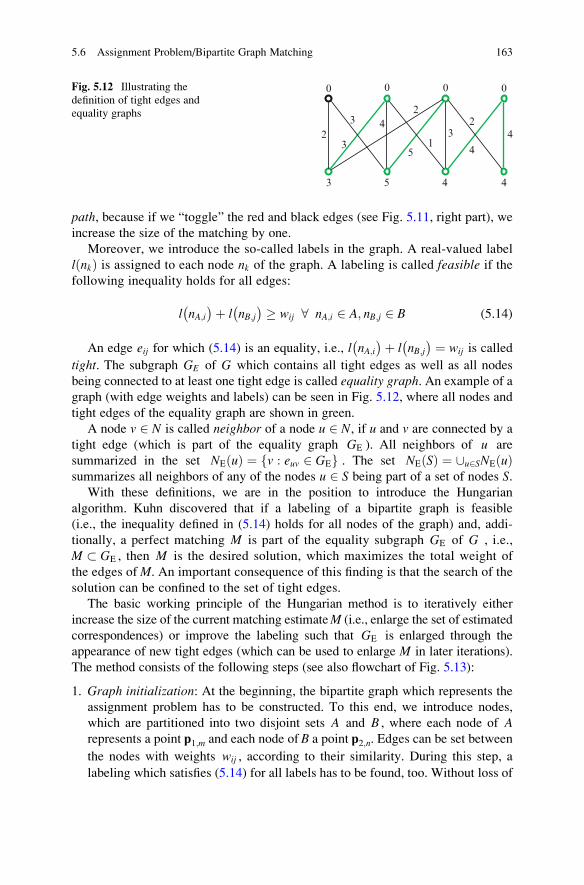
path, because if we “toggle” the red and black edges (see Fig. 5.11, right part), we

increase the size of the matching by one.

Moreover, we introduce the so-called labels in the graph. A real-valued label

l nkð Þ is assigned to each node nk of the graph. A labeling is called feasible if thefollowing inequality holds for all edges:

l nA;i� �þ l nB;j

� � � wij 8 nA;i 2 A; nB;j 2 B (5.14)

An edge eij for which (5.14) is an equality, i.e., l nA;i� �þ l nB;j

� � ¼ wij is called

tight. The subgraph GE of G which contains all tight edges as well as all nodes

being connected to at least one tight edge is called equality graph. An example of a

graph (with edge weights and labels) can be seen in Fig. 5.12, where all nodes and

tight edges of the equality graph are shown in green.

A node v 2 N is called neighbor of a node u 2 N, if u and v are connected by a

tight edge (which is part of the equality graph GE ). All neighbors of u are

summarized in the set NEðuÞ ¼ v : euv 2 GEf g . The set NEðSÞ ¼ [u2SNEðuÞsummarizes all neighbors of any of the nodes u 2 S being part of a set of nodes S.

With these definitions, we are in the position to introduce the Hungarian

algorithm. Kuhn discovered that if a labeling of a bipartite graph is feasible

(i.e., the inequality defined in (5.14) holds for all nodes of the graph) and, addi-

tionally, a perfect matching M is part of the equality subgraph GE of G , i.e.,

M � GE , then M is the desired solution, which maximizes the total weight of

the edges ofM. An important consequence of this finding is that the search of the

solution can be confined to the set of tight edges.

The basic working principle of the Hungarian method is to iteratively either

increase the size of the current matching estimateM (i.e., enlarge the set of estimated

correspondences) or improve the labeling such that GE is enlarged through the

appearance of new tight edges (which can be used to enlarge M in later iterations).

The method consists of the following steps (see also flowchart of Fig. 5.13):

1. Graph initialization: At the beginning, the bipartite graph which represents the

assignment problem has to be constructed. To this end, we introduce nodes,

which are partitioned into two disjoint sets A and B , where each node of Arepresents a point p1;m and each node of B a point p2;n. Edges can be set between

the nodes with weights wij , according to their similarity. During this step, a

labeling which satisfies (5.14) for all labels has to be found, too. Without loss of

2

2

3

3 4

5

31

4

24

0 0 0

3 5 4 4


definition of tight edges and

equality graphs


generality, we can set the label of all nodes of set B to zero (see also Fig. 5.12,

where the nodes of set B are all placed in the top row of the graph). In order to

satisfy (5.14), the label for each of the nodes of set A can be chosen such that it

corresponds to the maximum weight of all edges which are connected to that

node: 8nA;i 2 A : l nA;i� � ¼ max

nB;j2Bwij (an example can be seen in Fig. 5.12). As a

consequence, each node nA;i is connected to at least one tight edge. We can

choose as subset of these tight edges as initial matching M.

2. Iteration initialization: The method works on two node sets S and T . At thebeginning of each iteration, let be T ¼ fg (empty) and initialize S with one

arbitrarily picked node u of set A: S ¼ uf g; u 2 A. Additionally, u has to meet the

condition that it is free, i.e., that it is connected to at least one tight edge and that

it is not part of the current matching M. Informally speaking, the set S contains

points inAwhich are endpoints of potential matching extensions, whereas the set

T contains points in Bwhich are validated to be already part of the matching and

therefore must not be used for new matching edges.

3. Neighborhood definition: In this step, we calculate NEðSÞ, which is the set of all

nodes which are neighbors to a node of S. By comparing NEðSÞ with T, we’re inthe position to determine whether the matching or the labeling has to be updated.

Given that nodes of S serve as endpoints of potential matching extensions,NEðSÞcontains the endpoints “on the other side” of potential new matching edges. In

order to determine whether the labeling or the matching has to be updated, we

compare NEðSÞ with T (see step 4 and 5).

4. Label update: If NEðSÞ ¼ T , all potential “counterparts” of new matching

candidates of A already are part of the current matching. Therefore, we update

S

E

yes

no

Init bipar-tite graph

Update la-beling of

nodes

Init sets Sand T if

necessary

CalculateNE(S)

NE (S) == T ?

Is M a per-fect matching ?

Updatematching Mif possible

yes

no

Fig. 5.13 Flowchart of the Hungarian algorithm


the labels with the goal to create new tight edges (in other words, we enforce

NEðSÞ 6¼ T ), which will be useful when extending the matching in later

iterations. This is done with the following update rule, which is applied to all

nodes n of the graph:

Δ ¼ minx2S;y=2T

lðxÞ þ lðyÞ � wxy

� �

lnewðnÞ ¼lðnÞ � Δ if n 2 S

lðnÞ þ Δ if n 2 T

lðnÞ otherwise

8><>:

ð5:15Þ

After this update, we go on with step 3 (Recalculation of NEðSÞ).5. Matching update: If NEðSÞ 6¼ T , it could be possible to extend the matching.

Therefore, we arbitrarily pick a node y 2 NEðSÞ � T. If y is already matched to a

node z, we must not take it as a new endpoint of an additional matching edge.

Therefore, we extend the setsS ¼ S [ zf g andT ¼ T [ yf g (i.e., enlarge the setTcontaining all nodes validated to be already matched to some other node by y)and go on with the next iteration (step 3). If y is free, we’re in the position to

extend the matching. According to the above assumptions and definitions, the

path from u to y has to be an augmenting path (alternation between tight edges

which are part ofM and not part ofMwith two free endpoints). Therefore, we can

extend the matching by one edge if we alternate the affiliation of all edges of the

path fromu toy: if an edgeeij 2 M, we exclude it fromM, ifeij=2M, we include it in

M. Finally, the size of M is increased by one edge.

6. Convergence check: Stop if M is a perfect matching. Otherwise continue

with step 2

A toy example which illustrates the mode of operation of the Hungarian

method can be seen in Table 5.3. The bipartite graph shown there consists of

two node sets A ¼ nA;i� �

; i ¼ 1; 2; 3; 4f g (bottom row of each graph) and B ¼nB;j

� �; j ¼ 1; 2; 3; 4f g (top row of each graph), which are in some way connected

by some edges with weights given next to each edge (see left graph of top row).

In the first step, an initial feasible labeling has to be found according to the

proceeding explained above. According to the initial labeling, the graph contains

four tight edges, from which two are selected more or less arbitrarily as being part

of the initial matching This can be seen in the right graph of top row, where

matching edges are in red; tight edges not being part of the matching are indicated

by green color. Before we describe the proceeding of the method in detail, let’s

clarify the meaning of the different colors used in Table 5.3, which hopefully help

to understand the method:

• Red edge: Part of the current matching (is therefore tight, too)

• Green edge: Tight edge but not part of the current matching

• Bold edge: Edge where an important change happens

• Dark yellow node: Node being part of set S• Light blue node: Node being part of set NEðSÞ


• Node framed blue: Node which is considered during the calculation of the label

update Δ.• Colored labels: Labels which have just been updated

• Dashed edges: Augmenting paths where the matching has been updated

Table 5.3 Illustrating the working principle of the Hungarian method

2

2

3

3 4

5

31

4

2

4

nA,1 nA,2 nA,3nA,4

nB,1 nB,2 nB,3 nB,4 0

4

2

2

3

3 4

5

31

4

2

4

0 0 0

3 5 4

0

4

2

2

3

3 4

5

31

4

2

4

0 0 0

3 5 4

000 0

44

2

2

3

3 4

5

31

4

2

4

3 5

3 3

2

2

3

3 4

5

31

4

2

4

0 0 0

3 5

1

33

2

2

3

3 4

5

31

4

2

4

0 0 0

3 5

1

2

2

3

3 4

5

31

4

2

4

0 0 1

3 4 2 2

2

2

2

3

3 4

5

31

4

2

4

0 0 1

3 4 2 2

2

2

2

3

3 4

5

31

4

2

4

0 1 2

2 3 1 1

3

2

2

3

3 4

5

31

4

2

4

0 1

2 3 1 1

32

For details, see text


The iteration is initialized with the sets S ¼ nA;3� �

(dark yellow node) and

T ¼ fg . Based on S , the neighborhood is defined by NEðSÞ ¼ nB;4� �

(Conse-

quently, nB;4 is marked light blue node, see right part of top row of Table 5.3). As

NEðSÞ 6¼ T, we can try to extend the matching. Because nB;4 is a free node, this ispossible and the path between nA;3 and nB;4 is augmented. As this path contains

only one edge, we just have to include the said edge into the matching in this

simple case (see the bold edge in the left graph of the second row, which

switches its color from green to red).

Now we can redefine the node sets according to S ¼ nA;4� �

and T ¼ fg .Therefore, NEðSÞ ¼ nB;4

� �and again NEðSÞ 6¼ T (see left graph in the second

row). This time, however, y ¼ nB;4 is not free any longer. It is matched to z ¼ nA;3instead. Therefore, we enlarge S ¼ nA;3; nA;4

� �and T ¼ nB;4

� �. This leads to NE

ðSÞ ¼ nB;4� �

(c.f. right graph of second row). Now NEðSÞ ¼ T, which means that

we will update the labeling of all nodes of S and T. To this end, the update valueΔhas to be determined according to (5.15).Δ is calculated under consideration of all

nodes framed blue in the right graph of the second row and their connections and is

therefore set to 1.

The new labeling can be seen in the left graph of the third row (all colored values

have been updated). The label update has caused the emergence of an additional tight

edge (bold green). As a result, the neighborhood is enlarged to NEðSÞ ¼ nB;3; nB;4� �

.

This means that NEðSÞ 6¼ T (indicating an update of the matching), but nB;3 ¼ NEðSÞ�T is already part of the matching. Consequently, we enlarge S ¼ nA;2; nA;3; nA;4

� �

and T ¼ nB;3; nB;4� �

(right graph of the third row). Now NEðSÞ ¼ T and we perform

another label update step based on all nodes framed blue (again, Δ is set to 1). This

leads to a new labeling, another tight edge (bold green) and the updated NEðSÞ ¼nB;2; nB;3; nB;4

� �(left graph of fourth row).

Thus, NEðSÞ 6¼ T , and as nB;2 ¼ NEðSÞ � T is already part of the matching, no

matching update is to be performed (analogously to before). Instead, we enlarge

S ¼ nA;1; nA;2; nA;3; nA;4� �

and T ¼ nB;2; nB;3; nB;4� �

(right graph of the fourth row).

As a consequence,NEðSÞ ¼ T, which indicates one more label update step based on

all nodes framed blue (Δ is set to 1). This leads to a new labeling, two new tight

edges (bold green) and the updated NEðSÞ ¼ nB;1; nB;2; nB;3; nB;4� �

(left graph of

bottom row).

Accordingly, NEðSÞ 6¼ T, but in contrast to the previous steps, nB;1 ¼ NEðSÞ � Tis free. Therefore, we have an augmenting path from nB;1 to nA;4, both of which are

free endpoints (the path is indicated by dashed edges). Consequently, we can

“toggle” each edge of the path, which leads to a new matching (see red edges in

right graph of bottom row). Finally, this new matching is complete and we’re

finished. The total matching weight is 13.

The overall complexity is O n3ð Þ , with n being the cardinality of the two

point sets.


Please note that the algorithm given above maximizes the sum of the weightswij

of the matching. Many problems involve evaluating costs cij associated with each

correspondence though, and thus the algorithm should minimize the sum of the

weights of the matching. However, the minimization problem can easily be

converted to a maximization problem by calculating the weights wij as differences

cmax � cij, where cmax is chosen sufficiently large in order to ensure that all wij are

positive. Hence, small costs result in large weights.

In its initial form, the Hungarian algorithm can only match point sets of equal

size, because it determines a matching for every node of the graph. However, the

method can easily be extended to point sets of different size by the introduction of

the so-called dummy nodes. For example, if the cardinalityK ofP1 is larger than the

cardinality L ofP2 (i.e.,K � L ¼ D), the introduction ofD dummy nodes in node set

B ensures that both node sets are of equal size. If a node of set A is matched to a

dummy node, this means that it has no corresponding point in practice. Moreover,

we can introduce some additional dummy nodes in both sets in order to allow

unmatched points for both sets.

Each dummy node is connected to every node of the other set (such that every of

those nodes could be connected to a dummy node). The weight of those edges can

be set to tsim, which defines the minimum similarity two nodes must have in order to

be matched during recognition.

Pseudocode

function bipartiteGraphMatching (in point set 1

P1 ¼ p1;m;m 2 1; . . . ;K½ �� , in point set 2 P2 ¼ p2;n; n 2 1; . . . ; L½ ��

, in

number of dummy nodes D, in minimum similarity tsim, out per-fect matching M

// initialization of bipartite graphNum max K; Lð Þ þ D // at least D dummy nodes in each setfor m ¼ 1 to K // node set A

for n ¼ 1 to L // node set B

calculate similarity fsim between p1;m and p2;n, e.g. χ2-distance between descriptors d1;m and d2;nwmn fsim

nextnextfill graph with dummy nodes and connect each dummy node to eachnode of the other set with edge weight wd ¼ tsim.

// initial edge labelingfor i ¼ 1 to Num

l nA;i� � max

nB;j2Bwij

l nB;i� � 0

nextchoose initial matching M as a subset of all tight edges


// main iteration loopbInitSets truerepeat

// initialization of S and T, if necessaryif bInitSets ¼¼ true then

for i ¼ 1 to Numif nA;i is free then

S nA;i� �

i Num // a free node in A is found! stopend if

nextT fgbInitSets false

end if// calculation of NEðSÞfor all nodes of S (index r)

for all edges ert connecting nA;rif ert is a tight edge and nB;t=2NEðSÞ then

NEðSÞ NEðSÞ [ nB;t� �

end ifnext

next// check whether matching or labeling is to be updatedif NEðSÞ ¼¼ T then

// update labeling

Δ minx2S;y=2T

lðxÞ þ lðyÞ � wxy

� �

for i ¼ 1 to Numif nA;i 2 S then

l nA;i� � l nA;i

� �� Δend ifif nB;i 2 T then

l nB;i� � l nB;i

� �þ Δend if

nextelse // update matching, if possible

arbitrarily pick a node y 2 NEðSÞ � Tif y is free then

for all edges eij on path from u to yif eij 2 M then

M M � eij� �

else

M M [ eij� �

end if


nextbInitSets true // restart iterationelse // y is already matched to some node z

S S [ zf gT T [ yf g

end ifend if

until M is a perfect matching (all nodes belong to exactlyone element of M)

5.6.2 Example: Shape Contexts

One example of solving the correspondence problem with bipartite graph matching

is a method for object recognition proposed by Belongie et al. [1]. The objects are

recognized by utilizing an object model learned in a training phase. This object

model is based on the so-called shape contexts, which are descriptors being built on

the shapes of the object to be recognized. Briefly speaking, each shape context

represents the spatial distribution of points being located on the object contour in a

local neighborhood around one of those contour points (also called landmarkpoints”).

As we will see soon, bipartite graph matching is utilized in [1] in order to find

correspondences between the shape contexts extracted from a scene image under

investigation and shape contexts from the object model. Once the correspondences

are estimated, the algorithm derives the parameters of a transformation between the

two sets of shape contexts as well as a measure of similarity between the scene

image shape context set and the model set. Based on this similarity measure, it is

possible to distinguish between different kinds of objects: we simply can calculate

the similarity measure for all models of a model database. The model with the

highest score is considered as recognized if the score is above a certain threshold.

Bipartite graph matching should enable the algorithm to robustly find a consistent

matching set which contains no or at least very few outliers, such that the subsequent

transformation estimation ought to be successful. Before we take a closer look at how

bipartite graph matching is employed in the method, let’s first introduce the concept

of shape context as well as the general algorithm flow of the method.

In order to understand the working principle of shape contexts, we assume that

the object is represented by a set of so-called contour points, which are located at

positions with rapid local changes of intensity. At each contour point, a shape

context can be calculated. Each shape context defines a histogram of the spatial

distribution of other landmark points relative to the current one. These histograms

provide a distinctive characterization for each landmark point, which can be used as

a descriptor.

A shape context example is depicted in Fig. 5.14: in the left part, sampled contour

points of a handwritten character “A” are shown. At the location of each of them, the


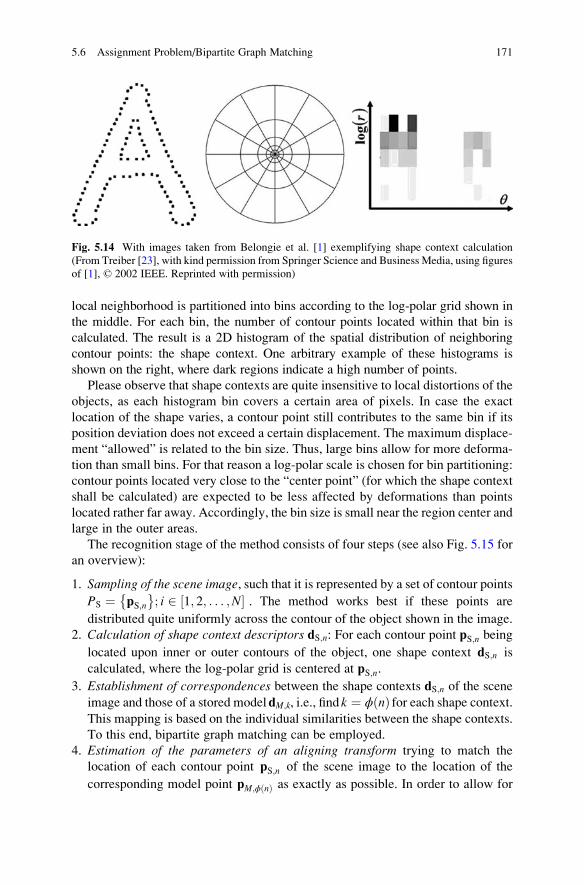
local neighborhood is partitioned into bins according to the log-polar grid shown in

the middle. For each bin, the number of contour points located within that bin is

calculated. The result is a 2D histogram of the spatial distribution of neighboring

contour points: the shape context. One arbitrary example of these histograms is

shown on the right, where dark regions indicate a high number of points.

Please observe that shape contexts are quite insensitive to local distortions of the

objects, as each histogram bin covers a certain area of pixels. In case the exact

location of the shape varies, a contour point still contributes to the same bin if its

position deviation does not exceed a certain displacement. The maximum displace-

ment “allowed” is related to the bin size. Thus, large bins allow for more deforma-

tion than small bins. For that reason a log-polar scale is chosen for bin partitioning:

contour points located very close to the “center point” (for which the shape context

shall be calculated) are expected to be less affected by deformations than points

located rather far away. Accordingly, the bin size is small near the region center and

large in the outer areas.

The recognition stage of the method consists of four steps (see also Fig. 5.15 for

an overview):

1. Sampling of the scene image, such that it is represented by a set of contour points

PS ¼ pS;n� �

; i 2 1; 2; . . . ;N½ � . The method works best if these points are

distributed quite uniformly across the contour of the object shown in the image.

2. Calculation of shape context descriptors dS;n: For each contour point pS;n being

located upon inner or outer contours of the object, one shape context dS;n is

calculated, where the log-polar grid is centered at pS;n.

3. Establishment of correspondences between the shape contexts dS;n of the sceneimage and those of a stored modeldM;k, i.e., findk ¼ ϕðnÞ for each shape context.This mapping is based on the individual similarities between the shape contexts.

To this end, bipartite graph matching can be employed.

4. Estimation of the parameters of an aligning transform trying to match the

location of each contour point pS;n of the scene image to the location of the

corresponding model point pM;ϕðnÞ as exactly as possible. In order to allow for

Fig. 5.14 With images taken from Belongie et al. [1] exemplifying shape context calculation

(From Treiber [23], with kind permission from Springer Science and Business Media, using figures

of [1], © 2002 IEEE. Reprinted with permission)


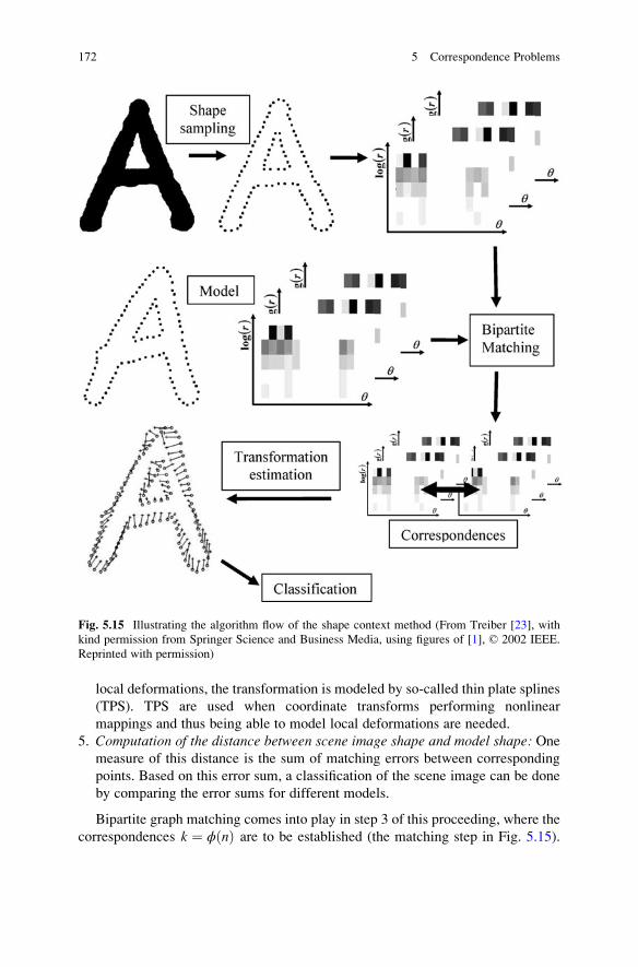
local deformations, the transformation is modeled by so-called thin plate splines

(TPS). TPS are used when coordinate transforms performing nonlinear

mappings and thus being able to model local deformations are needed.

5. Computation of the distance between scene image shape and model shape: Onemeasure of this distance is the sum of matching errors between corresponding

points. Based on this error sum, a classification of the scene image can be done

by comparing the error sums for different models.

Bipartite graph matching comes into play in step 3 of this proceeding, where the

correspondences k ¼ ϕðnÞ are to be established (the matching step in Fig. 5.15).

Fig. 5.15 Illustrating the algorithm flow of the shape context method (From Treiber [23], with

kind permission from Springer Science and Business Media, using figures of [1], © 2002 IEEE.

Reprinted with permission)


Therefore, we focus on this step and refer the interested reader to [1] for a detailed

description of the other steps.

In order to find the correspondences, the problem has to be formulated as a

bipartite graph. Accordingly, each landmark point is represented as a node in the

graph, where all scene image landmark points pS;n are collected in a node set A and

all model landmark pointspM;k in a second setB. Edges are established only between

nodes of different sets. Without the usage of any prior knowledge, each pS;n is

connected to all pM;k by the edges enk.

Moreover, a cost cnk can be calculated for each edge based on the dissimilarity

between the shape contextsdS;n anddM;k. To this end, the χ2 test metric is suggested,

which is given by

cnk ¼ 1

2

XR

r¼1

dS;nðrÞ � dM;kðrÞ� �2

dS;nðrÞ þ dM;kðrÞ (5.16)

where dðrÞ is the rth element of the descriptor vector d. Possible modifications

aim at considering further aspects in the costs cnk, e.g., appearance similarities,

which can be measured by normalized cross correlations of image patches

around each landmark point. Observe that (5.16) is a measure of dissimilarity,

i.e., in order to find the correct correspondence (5.16) has to be minimized. If

we want to convert the problem into a maximization problem, a weight wnk can

be set such that wnk ¼ cmax � cnk.The resulting bipartite graph matching problem can now be solved with the

Hungarian method presented in the previous section. Belongie et al. [1], however,

suggested to use the method of [11], which was considered to be more efficient in

this case by the authors. Additionally, the total similarity value of the found

matching can be utilized in a subsequent classification step (step 5 of the above

proceeding).

Observe that with bipartite graph matching all correspondences are estimated

through a joint optimization, whereas iterative methods like ICP search the best

correspondence for each element individually. As a consequence, the estimated

correspondences should contain less outliers, and, therefore, no iterative proceeding

is needed; the aligning transform can (hopefully) be estimated reliably in a single step.

The authors of [1] tested object recognition with shape contexts in different

applications, such as handwritten digit recognition and trademark retrieval.

Figure 5.16 presents some of their results for trademark retrieval. The left icon of

each group is the query trademark, whereas the three icons to the right of the query

icon show the top three most similar icons of a model database as suggested by the

algorithm. The numbers given below indicate the distance calculated by the system.

A very recent approach of estimating the correspondences between two 3D

shapes uses bipartite graph matching as a building block (see [20]). There, the

point set to be matched is sampled from a mesh representation of the shapes. The

method does not make use of descriptors; the weights of the bipartite graph, which


indicate the probabilities that two points from different shapes correspond to each

other, are derived from a spectral embedding of the sampled mesh points (as

described earlier in this chapter, c.f. [10]) instead.

Subsequently, the correspondences are estimated in an iterative Expectation-

Maximization (EM) algorithm. In the M-Step the correspondences are estimated

via bipartite graph matching, followed by a refinement step which also allows for

many-to-one mappings. The E-Step updates the weights of the bipartite graph, i.e.,

the probabilities that two points form a correspondence. M-Step and E-Step are

performed in alternation until convergence.

The combination of various methods (spectral embedding, bipartite graph

matching, iterative refinement) into one framework results in very accurate results,

as was shown in [20]. In order to get an impression of the performance, the

interested reader is referred to the figures presented in the original article [20].

References

1. Belongie S, Malik J, Puzicha J (2002) Shape matching and object recognition using shape

contexts. IEEE Trans Pattern Anal Mach Intell 24(4):509–522

2. Besl PJ, McKay ND (1992) A method for registration of 3-D shapes. IEEE Trans Pattern Anal

Mach Intell 14(2):239–256

Fig. 5.16 Illustrating the performance of the algorithm in the context of trademark retrieval (©2002 IEEE. Reprinted, with permission, from Belongie et al. [1])


3. Choi S, Kim T, Yu W (2009) Performance evaluation of RANSAC family. In: Proceedings of

the British machine vision conference, London, pp 81.1–81.12

4. Duchenne O, Bach F, Kweon I-S, Ponce J (2011) A tensor-based algorithm for high-order

graph matching. IEEE Trans Pattern Anal Mach Intell 33:2383–2395

5. Egozi A, Keller Y, Guterman H (2013) A probabilistic approach to spectral graph matching.


6. Fishler MA, Bolles RC (1981) Random sample consensus: a paradigm for model fitting with

applications to image analysis and automated cartography. Mag Commun ACM 24

(6):381–395

7. Fitzgibbon AW (2003) Robust registration of 2D and 3D point sets. Image Vis Comput 21

(13–14):1145–1153

8. Harris C, Stephens M (1988) A combined corner and edge detector. In: Alvey vision confer-

ence, Manchester, pp 147–151

9. Hartley R, Zisserman A (2004) Multiple view geometry in computer vision, 2nd edn.

Cambridge University Press, Cambridge. ISBN 978–0521540513

10. Jain V, Zhang H (2006) Robust 3D shape correspondence in the spectral domain. IEEE Int

Conf Shape Model Appl 118–129

11. Jonker R, Volgenant A (1987) A shortest augmenting path algorithm for dense and sparse

linear assignment problems. J Comput 38:325–340

12. Kuhn HW (1955) The Hungarian method for the assignment problem. Nav Res Logist Q

2:83–87

13. Leordeanu M, Herbert M (2005) A spectral technique for correspondence problems using

pairwise constraints. In: Proceedings of the 10th IEEE international conference on computer

vision, vol 2, Beijing, pp 1482–1489

14. Lowe DG (2004) Distinctive image features from scale-invariant viewpoints. Int J Comput Vis

60:91–111

15. Marquardt D (1963) An algorithm for least-squares estimation of nonlinear parameters. SIAM

J Appl Math 11(2):431–441

16. Mikolajczyk K, Schmid C (2005) A performance evaluation of local descriptors. IEEE Trans

Pattern Anal Mach Intell 27(10):1615–1630

17. Mikolajczyk K, Tuytelaars T, Schmid C, Zisserman A, Matas J, Schaffalitzky F, Kadir T, Van

Gool L (2005) A comparison of affine region detectors. Int J Comput Vis 65:43–72

17. Munkres J (1957) Algorithms for assignment and transportation problems. J Soc Ind Appl

Math 5(1):32–38

18. Rubner Y, Tomasi C, Leonidas JG (2000) The earth mover’s distance as a metric for image

retrieval. Int J Comput Vis 40(2):99–121

19. Rummel P, Beutel W (1984) Workpiece recognition and inspection by a model-based scene

analysis system. Pattern Recognit 17(1):141–148

20. Sahilloglu Y, Yemez Y (2012) Minimum-distortion isometric shape correspondence using EM

algorithm. IEEE Trans Pattern Anal Mach Intell 34(11):2203–2215

21. Schmid C, Mohr R (1997) Local grey value invariants for image retrieval. IEEE Trans Pattern

Anal Mach Intell 19:530–535

22. Trefethen LN, Bau D (1997) Numerical linear algebra. Society for Industrial and Applied

Mathematics, Philadelphia. ISBN 978-0898713619

23. Treiber M (2010) An introduction to object recognition – selected algorithms for a wide

variety of applications. Springer, London. ISBN 978–1849962346

References 175

Chapter 6

Graph Cuts

Abstract Energy functions consisting of a pixel-wise sum of data-driven energies

as well as a sum of terms affected by two adjacent pixels (aiming at ensuring

consistency for neighboring pixels) are quite common in computer vision. This kind

of energy can be represented well by Markov Random Fields (MRFs). If we have to

take a binary decision, e.g., in binary segmentation, where each pixel has to be

labeled as “object” or “background,” the MRF can be supplemented by two

additional nodes, each representing one of the two labels. The globally optimal

solution of the resulting graph can be found by finding its minimum cut (where the

sum of the weights of all severed edges is minimized) in polynomial time by

maximum flow algorithms. Graph cuts can be extended to the multi-label case,

where it is either possible to find the exact solution when the labels are linearly

ordered or the solution is approximated by iteratively solving binary decisions.

An instance of the max-flow algorithm, binary segmentation, as well as stereo

matching and optical flow calculation, which can both be interpreted as multi-

labeling tasks, is presented in this chapter. Normalized cuts seeking a spectral, i.e.,

eigenvalue solution, complete the chapter.

6.1 Binary Optimization with Graph Cuts

6.1.1 Problem Formulation

Many computer vision problems can be modeled by a Markov Random Field(MRF), because MRFs are well suited for representing a class of energy functions

which are of widespread use in computer vision. These energy functions mainly

consist of two terms (cf. (6.1)):

• A data-driven term Ed, where we can evaluate for each pixel p (represented by anode in the MRF) how well our estimations correspond to the observed data.



177

• Interaction potentials Eint between adjacent pixels (nodes of the MRF), which

measure the “consistency” between estimations of adjacent pixels p and q, e.g.,all pixels within a 4-neighborhood .

ð6:1Þ

Consider a binary segmentation task, for example, where we want to partition an

image into object and background, i.e., we have to decide for each pixelpwhether itcan be classified as “object” or “background.” Informally speaking, a “good”

segmentation is obtained when all pixels of the same class have similar intensities

(or colors) and if the boundaries between pixels labeled as “object” and “back-

ground” are located such that adjacent pixels of different labels have dissimilar

intensities/colors. The mapping of these criteria to the two terms of the energy of

(6.1) is straightforward as follows:

• Ed measuring data fidelity can be derived from an evaluation how well the

observed data at pixel p fits into intensity/color statistics obtained from pixels

with known labeling, which could, e.g., be brightness histograms or Gaussian

mixture models of color distributions.

• The interaction potentials Eint , which measure the cost of assigning different

labels to adjacent pixels, can be based on the intensity or color difference

between adjacent pixels p and q (e.g., where q is located within a 4-neighborhoodaround p). High differences are mapped to low costs and vice versa.

This kind of energy function can be modeled by an MRF, where each pixel p is

represented by a node (see Fig. 6.1 for a small example covering just 3 � 3 pixels).

In accordance to the pixel grid, these nodes are arranged in a rectangular

two-dimensional grid. Adjacent nodes p and q are connected by an edge epq(black lines in Fig. 6.1). For example, a node p can be connected to all nodes withinits 4-neighborhood. Another common choice is connecting all nodes within an 8-

neighborhood. The weight wpq of each edge epq represents the interaction potentialsEint p; qð Þ between adjacent pixels.wpq should be high when the intensities/colors of


topology of a two-terminal

graph (left), for which a

minimum cut is to be

calculated (right, cut ingreen)

178 6 Graph Cuts

p and q are similar. The numerical value of the weights is indicated by the thickness

of the connections in Fig. 6.1.

In order to incorporate the data-driven terms Ed , two additional so-called

terminal nodes (one “source” node s and one “sink” t ) are introduced. Every

nonterminal node can be connected to s as well as t by additional edges eps and ept.These edges are also called t-links (terminal links), whereas edges between two

nonterminal nodes are called n-links (neighborhood links). Each terminal node

represents a label, e.g., for binary segmentation s can be chosen as “object terminal”

and t as “background terminal.”

The weights wps reflect the fidelity of the intensity/color at pixel p to the object

pixel statistics (andwpt the fidelity to the statistics of the background pixels). Hence,

wps should be high (andwpt low) if the data observed atpfits well into the statistics ofall known object pixels. Respectively, wps should be low (and wpt high) when the

appearance at p is in accordance with background appearance.

As a summary, the whole setting is described by a graph G ¼ N;Eð Þ consistingof nonterminal nodes representing the pixels of the image, two terminal nodes

representing the two labels “object” and “background,” as well as edges connecting

the nodes, whose weights represent the energies as defined in (6.1).

A binary segmentation of the image can now be represented by a so-called

graph cut. A cut C of a graph is a subset of edges (C � E), which separate the

node set N of the graph into two disjoint subsets A and B, i.e., N ¼ A [ B and

A \ B ¼ fg.C defines a valid binary segmentation if the two terminals are contained

in different subsets. This implies that each nonterminal node remains either

connected to s or t, which can be interpreted as follows: if the node of a pixel still

is connected to s, it is classified as “object”; if it remains connected to t, it is assignedto the “background” label.

For each cutC, we can define a so-called cut functionEC, which can be set to the

sum of the weights of the edges it severs:

EC ¼X

e2Cwe (6.2)

Consequently, the optimal segmentation can be found if we find the minimum

cut, e.g., the subset of edges which minimizes (6.2):

C� ¼ argminX

e2Cwe (6.3)

In the general case, the problem of finding the minimum cut is NP-hard, but for

the special case of two terminals, it has been proven that the minimum cut can be

found in polynomial time. Efficient algorithms are presented in the next section.

The main advantage of graph cuts is that in contrast to many other methods, it is

possible to find a global optimum of the energy function defined in (6.1) if

appropriate algorithms are employed to find the minimum cut. Moreover, the

computational complexity of the worst case is quadratic with the number of pixels

6.1 Binary Optimization with Graph Cuts 179

and in practice allows a rather fast optimization for typical image sizes. However,

up to now, as we just have two terminals, only binary decisions can be modeled by

graph cuts.

In fact, Grieg et al. [13] were the first to introduce graph cuts in computer vision

applications by proposing to solve the problem of restoring binary images with

graph cuts. Probably mainly due to this restriction, their work remained unnoticed

for a long time. However, in the meantime it was discovered that a fairly large

amount of vision problems can be tackled by binary decisions, and, furthermore,

graph cuts can be extended to a multi-label case efficiently. As a consequence, this

field became a quite active area of research over the last decade.

6.1.2 The Maximum Flow Algorithm

Now that we know how to build a graph representing energy functions for binary

labeling problems in the form of (6.1), let’s turn to the question how to find the

minimum cut of the graph. Please note that most algorithms do not try to solve the

optimization problem of (6.3) directly. Instead, they seek for the so-called maxi-

mum flow through the graph, which was shown by Ford and Fulkerson [9] to yield

the same solution as finding the minimum cut.

Here, the edges of the graph are interpreted as “pipes,” which can be used to

pump water through them. The maximum total amount of water which can be

pumped from the source to the sink is called the maximum flow. The weight of each

edge can be interpreted as the “capacity” defining the maximum amount of water

which can run through the corresponding pipe segment. An edge is called

“saturated” if it contains as much water as possible and, consequently, there is no

spare capacity left. We can increase the total flow through the graph until the

maximum flow is found. At that point, every possible path from s to t contains atleast one saturated edge, because if there would exist a path where every segment

has spare capacity left, we could further increase the flow.

According to Ford and Fulkerson, the maximum flow solution, which yields a set

of saturated edges, is equivalent to the minimum cut solution. After calculating the

maximum flow, the set of saturated edges directly leads to the minimum cut

solution (if a unique solution exists) as follows: If we exclude all saturated edges

from the graph, every nonterminal node remains connected either to the source or

the sink. Consequently, the set of saturated edges partitions the graph into two

disjoint node subsets. Consequently, all former edges between nodes belonging to

different subsets must be part of the minimum cut.

Informally speaking, evidence for equivalence of the maximum flow and mini-

mum cut solution is given because of two reasons:

• Every path from s to t has to contain at least one saturated edge. Otherwise, therewould be some capacity left at each pipe segment of the path and we could

increase the flow. The fact that there is at least one saturated edge in every path

180 6 Graph Cuts

from s to t ensures the fact that s and t are contained in different subsets of the

partitioned graph.

• Pipes with small capacity are expected to saturate soon as the flow through the

graph increases. This corresponds to the fact that the minimum cut should

contain many edges with small weight.

Basically, there are two main classes of algorithms intending to find the maxi-

mum flow:

• Augmenting path algorithms: This type dates back to the article of Dinic [8] and is

an iterative procedure, which maintains a “valid” flow at each iteration. In order to

be a valid solution, the incoming flow has to be equal to the outgoing flow at every

node of the graph. Starting from zero flow, these methods try to iteratively

increase (“augment”) the total flow by first identifying a path with spare capacity

left and then increasing the flow through this path as much as possible in each

iteration step. The iteration terminates when no more increase is possible.

• Push/relabel algorithms introduced by Goldberg [11] allow the nodes to have a

flow “excess,” when the incoming flow is larger than the outgoing flow. As the

occurrence of an excess represents an invalid total flow, the excess has to be

eliminated again at some point of the proceeding. To this end, the algorithm

seeks to distribute the excess occurring at a node among its neighbors. Without

going into details here, we refer the interested reader to [7], which gives a good

explanation of this class of algorithms.

In the following, we want to present the algorithm of Boykov and Kolmogorov

[3], which falls into the class of augmenting path algorithms and tries to reuse

information gathered at previous iterations during the search for paths with spare

capacity. While it is commonly accepted that push/relabel algorithms perform best

for general graph cut applications, the authors of [3] experimentally showed that

their algorithm outperformed other max-flow methods in the special context of

typical vision applications.

As already mentioned, augmenting path algorithms fall into the class of iterative

procedures, where in each iteration a path from s to twith spare capacity is identifiedfirst. Next, we can try to increase the flow along this path as much as possible. The

iteration stops when no more growth of the flow is possible. Because the total flow

is augmented at each step (and never reduced), the algorithm is guaranteed to

converge.

In order to identify paths with spare capacity in an efficient manner, the algorithm

maintains two data structures, a so-called residual graph and a search tree:

• The residual graph has the same topology as the graph to be optimized, but in

contrast to the “main” graph, the weights of its edges are set to the spare capacity

which can be used to augment the flow along these edges. At start (where the

total flow is zero), the residual graph is identical to the main graph. As iteration

proceeds, the weights of its edges will successively be reduced. As a conse-

quence, saturated edges will disappear, because their spare capacity (and conse-

quently their weight in the residual graph) will be zero. With the help of the


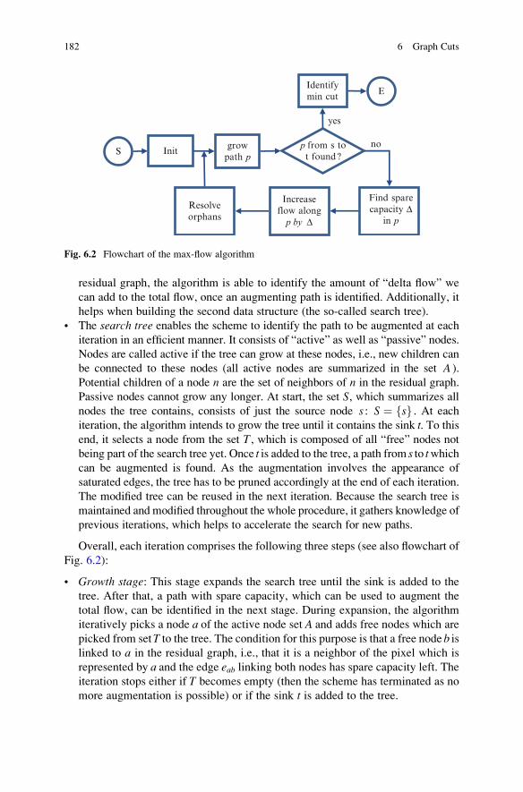
residual graph, the algorithm is able to identify the amount of “delta flow” we

can add to the total flow, once an augmenting path is identified. Additionally, it

helps when building the second data structure (the so-called search tree).

• The search tree enables the scheme to identify the path to be augmented at each

iteration in an efficient manner. It consists of “active” as well as “passive” nodes.

Nodes are called active if the tree can grow at these nodes, i.e., new children can

be connected to these nodes (all active nodes are summarized in the set A ).

Potential children of a node n are the set of neighbors of n in the residual graph.

Passive nodes cannot grow any longer. At start, the set S, which summarizes all

nodes the tree contains, consists of just the source node s : S ¼ sf g . At eachiteration, the algorithm intends to grow the tree until it contains the sink t. To thisend, it selects a node from the set T, which is composed of all “free” nodes not

being part of the search tree yet. Once t is added to the tree, a path from s to twhichcan be augmented is found. As the augmentation involves the appearance of

saturated edges, the tree has to be pruned accordingly at the end of each iteration.

The modified tree can be reused in the next iteration. Because the search tree is

maintained and modified throughout the whole procedure, it gathers knowledge of

previous iterations, which helps to accelerate the search for new paths.

Overall, each iteration comprises the following three steps (see also flowchart of

Fig. 6.2):

• Growth stage: This stage expands the search tree until the sink is added to the

tree. After that, a path with spare capacity, which can be used to augment the

total flow, can be identified in the next stage. During expansion, the algorithm

iteratively picks a node a of the active node set A and adds free nodes which are

picked from setT to the tree. The condition for this purpose is that a free nodeb islinked to a in the residual graph, i.e., that it is a neighbor of the pixel which is

represented by a and the edge eab linking both nodes has spare capacity left. Theiteration stops either if T becomes empty (then the scheme has terminated as no

more augmentation is possible) or if the sink t is added to the tree.

S

E

Initgrowpath p

p from s tot found ?

Identifymin cut

yes

no

Find sparecapacity Δ

in p

Increaseflow along

p by Δ

Resolveorphans

Fig. 6.2 Flowchart of the max-flow algorithm

182 6 Graph Cuts

• Augmentation stage: Starting from t, the tree can be traced back to the source s,which allows us to identify the path p to be augmented: p consists of all nodes wepassed when tracing back the tree. The next task is to identify the smallest spare

capacity Δ along p . This can be done by evaluating the edge strengths of the

residual graph. Now we can augment the flow by adding Δ. Consequently, the

strength of all edges along p has to be reduced by Δ in the residual graph. Please

note that now at least one edge becomes saturated. Accordingly, all newly

saturated edges are removed from the residual graph and from the tree as well.

As a result, some nodes of the search tree become “orphans,” i.e., they don’t have a

parent any longer. These nodes are collected in the set O. In other words, the treesplits into a “forest,” where the newly emerged trees have some node ofO as root.

• Adaption stage: In this stage, the aim is to recover a single tree from the forest.

To this end, either a new parent has to be found for each orphan or, if this is not

possible, the orphan has to be removed from the tree and added to the set of free

nodes T. In that case, all of the children of that orphan have to be added toO (and

subsequently processed in the adaption stage) as well. This stage terminates

whenObecomes empty. In order to find a parent for an orphano 2 O, all nodesq,which are linked to o via a non-saturated edge, are checked. If q 2 S, and if the

tree to whichqbelongs to has the source s as root, thenq can be accepted as a newparent of o. If these conditions are met by none of the members, o is removed

from the tree and all children of o are added to O. These nodes are also added to

the active node set A (if they are not active already), because those nodes are

neighbors of o, which has just been added to the free node set. This means that

there exists a free neighbor for all those nodes, i.e., a possibility to expand the

tree, and consequently their status has to be set to “active.”

Pseudocode

function augmentingPathMinGraphCut (in graph G ¼ N;Eð Þ, outminimum cut C�)

// initializationS sf g // the only node of search tree is source nodeA sf g // the only active node is the source nodeT N � sf g // all other nodes are “free” nodesO fg // no “orphans”GR ¼ G // residual graph GR is equal to “main” graph

// main iteration looprepeat

// growth stagep ¼ fg // no augmenting path is known at this pointif t 2 S then // tree contains sink from previous step

trace back tree from t to s! identify and set path pend ifwhile p ¼¼ fg ^ A 6¼ fg // active nodes for expansion exist

randomly pick an active node a 2 A


for all non-saturated edges eaq linking ato some neighbor qif q 2 T then // q is a free node

S S [ qf g // add q to search treeA A [ qf g // q is an active nodeT T � qf g // remove q form free node setRemember a as parent of q (for backtracking)if q ¼¼ t then // path to sink found

trace back tree from t to s! identify pbreak // path found ! terminate while-loop ofgrowth stage

end ifend if

nextA A� af g // all neighbors of a are processed

end while

// augmentation stageif p 6¼ fg then // augmenting path is found: p not empty)

find smallest free capacity Δ along pupdate GR by decreasing all data weights along p by Δfor each edge eqr becoming saturated

O O [ rf g // r becomes an “orphan”next

// adaption stagewhile O 6¼ fg // orphans still exist and must beeliminated

randomly pick an orphan o 2 ObParentFound falsefor all non-saturated edges eqo linking a potential new

parent q of o to oif q 2 S and q is linked to source s then

// parent foundconnect o to q in search treebParentFound truebreak // abort for-loop as new parent is found

end ifnextif bParentFound ¼¼ false then // no parent found

S S� of g // remove o from treeA A� of g if o 2 A // free node can’t be activeT T [ of g // add o to free node setadd all children of o to the set of orphans Oadd all children of o to active node set A, if theycurrently are =2A

end if

184 6 Graph Cuts

O O� of g // o is processed nowend while

end ifuntil p ¼¼ fg // terminate when no augmentation path isfound

// find minimum cutC� fgfor all edges e 2 E

if e=2GR then // e is saturated (not part of GR)C� C� [ ef g // add e to minimum cut

end ifnext

6.1.3 Example: Interactive Object Segmentation/GrabCut

As alreadymentioned, graph cuts can be used for binary segmentation (see, e.g., [1, 2]),

where the task is to partition every pixel of an image into one of two sets (“object” and

“background”).

This task can be accomplished by finding the minimum cut of a graph G as

presented above, where the nodes are arranged in a rectangular grid. Each pixel

is represented by one node p , which is linked to its neighbors. In [2] an

8-neighborhood is used, but other topologies are possible. Additionally, Gcontains two terminal nodes, where the source s is called “object terminal” and

the sink t represents the “background terminal.”

A cut ofG, which partitions the node set into two disjoint subsets A and B, wheres and t are forced to belong to different subsets, defines a segmentation such that all

pixels remaining connected to s are considered to be classified as “object” pixels.

Accordingly, all pixels remaining connected to t are considered to be classified as

“background” pixels. The segmentation boundary is defined by all n-links between

two nonterminal nodes being severed by the cut. Observe that such a cut imposes no

topology constraints, i.e., the “object area” can be split into multiple regions, which

can also have holes, and so on.

A segmentation can be specified by a binary vector l, whose number of elements

is equal to the number of pixels. The entry lp 2 0; 1f g relating to pixel/node p is setto 1 if p belongs to the object region and set to 0 if p belongs to the background

region, respectively.

The “quality” of a segmentation can be measured by a cost function E lð Þconsisting of two terms:

ð6:4Þ

where λ is a weighting factor balancing the two terms. The two contributions of the

cost can be explained as follows:


• The regional term R lð Þ evaluates how well the pixels fit into the region they are

assigned to (which is defined by l). To this end, it sums up the contributions

Rp lp� �

of each pixel p (the Rp lp� �

sometimes are also called unary term, as they

are affected by only one pixel). A simple measure is how well the intensity (or

color) of p fits into an intensity (or color) distribution, which for now is assumed

to be known for both regions. TheRp’s should act as a cost: if the intensity Ip of pcorrelates well with the intensity distribution of the “object class,” Rpð1Þ shouldbe low (conversely, Rpð0Þ should be low if Ip fits well into the background

statistic). The Rp’s can be represented by the edge weights of the t-links in the

graph. For example, if Ip is in accordance with the “object distribution,” there

should be a strong link to the source (object) terminal s and a weak link to the

sink (background) terminal t . Therefore, the edge weight wpt of the edge

connecting p with the terminal is set to Rpð1Þ (which is low in case Ip fits wellinto the object intensity distribution and can therefore be severed at low cost).

The edge weight wps to the source is set to Rpð0Þ, respectively.• The boundary term B lð Þ defines the cost of assigning adjacent pixels to different

regions. It therefore consists of the sum of the contributions Bpq of all

combinations of pixels p and q located in a neighborhood , e.g.,

8-neighborhood. The δ-function ensures that we only count costs when p and qare assigned to different regions, i.e., lp 6¼ lq. A simple measure for Bpq is based

on the intensity difference between p and q: if Ip is similar to Iq, Bpq should be

high, because it is unlikely that adjacent pixels with similar appearance belong

to different regions. The Bpq can be represented by the edge weights wpq of the

n-links in the graph.

The aim of the segmentation algorithm is to find a segmentation l� such that E lð Þis minimized: l� ¼ argmin

lE lð Þ. In order to find l�, we can apply a minimum graph

cut algorithm, because – if we set the edge weights as just explained –E lð Þ is definedby the sum of the weights of all edges ofG being severed by a particular cut. Hence,

finding the minimum cut also reveals an optimal segmentation in the sense thatE lð Þis minimized.

Up to now, an open question is how to calculate the individual costs Rp and Bpq.

Considering the boundary costs Bpq, it can be assumed that the cost of a cut is high,

if the intensities of p and q are similar. This can be expressed by

Bpq ¼ exp � Ip � Iq� �2

2σ2

!� 1

d p; qð Þ (6.5)

where d p; qð Þ denotes the spatial distance between p and q. In a 4-neighborhood thisterm can be neglected, but in a 8-neighborhood it can be used to devalue the

diagonal relationships.

As desired, Bpq takes low values when Ip and Iq are quite different. However,

please note that intensity differences between single pixels are sensitive to camera

186 6 Graph Cuts

noise. Generally, it is not indented to obtain low values of Bpq because of noise.

Therefore, the factor σ is introduced. σ determines how much Ip and Iq have to differ

for a low cost. Roughly speaking, the cost is small if Ip � Iq�� < σ. Hence, a proper

value of σ can be derived from camera noise estimation.

As far as the regional terms Rp are concerned, we need to define a quantity

measuring how well the intensity Ip fits into intensity statistics of the object or back-

ground pixels. For the moment, let’s assume that we know the intensity histograms

HO of the “object” class and HB of the “background class,” respectively. After

appropriate smoothing,HO andHB can directly be interpreted as a probability that

a pixel with intensity I belongs to the corresponding class: P lp ¼ 1� � / HO Ip

� �and

P lp ¼ 0� � / HB Ip

� �, respectively. However, we need costs instead of probabilities.

Observe that probabilities can easily be converted into costs if we take the negative

logarithm of the probability distribution. Consequently, the Rp can be expressed as

Rp lp� � ¼ � ln ~HO Ip

� �� if lp ¼ 1

� ln ~HB Ip� ��

if lp ¼ 0

�(6.6)

where the ~HO and ~HB are smoothed and scaled versions (such that the sum of all

entries equals 1) of the intensity histograms. With (6.5) and (6.6) the graph is

completely defined. Its minimum cut can, e.g., be found by applying the method

described in the previous section.

But there still is the open question how to get knowledge about the distributions~HO and ~HB . In some applications, ~HO and ~HB can be derived from a priori

knowledge. However, this might not be possible in every case. Therefore, [2]

suggest an interactive procedure: At start, the user marks some pixels as “object”

and some as “background” by drawing brushes upon the image. Now the system

can derive the histograms from the regions covered by the brushes.

Because the marked pixels just have to be located somewhere within the object

and background regions, the exact position of the brush is not crucial. This fact

makes this type of user input rather convenient (compared, e.g., to a definition of

boundary pixels as necessary in the “intelligent scissors” method presented in the

next chapter, where the positions should be as accurate as possible).

Please note that there is a second way of making use of the brushes: In fact, the

pixels of the brushed regions have already been classified by the user. This

classification acts as “hard constraints” for the subsequent automatic segmentation,

as it must not be changed by the system. Consequently, we can set the Rp’s of those

pixels such that it is ensured that the label of those pixels remains unchanged.

Observe that these hard constraints simplify the problem, because the number of

unknowns is reduced.

An example of the performance of graph cut segmentation can be seen in

Fig. 6.3, where the segmentation result is indicated by the coloring. While the

original images are grayscale, the segmented background is colored blue, whereas

the object area is indicated by red color. The solid red and blue brushes indicate the

user input serving as hard constraints. As clearly can be seen, the method is capable


of accurately separating the object of interest from the background, even in the

presence of considerable texture in both regions.

Observe that the segmentation process can also be implemented as an interactive

update procedure: after a first “round” of user input, the system calculates the

minimum cut according to this input and presents the segmentation result to the

user. Now, the user can add additional brushes in order to refine the result. The

newly added brushes lead to new hard constraints and the graph is adjusted

accordingly by changing the weights of the affected t-links. Based on the former

solution, the system can now calculate a refined segmentation very quickly. Of

course, additional update steps are possible.

However, new user input leads to an altered segmentation result only if the user-

specified label differs from the automatic labeling. Moreover, the change of the

t-link weights might involve a reduction of weights such that the constraint that all

paths from the source terminal to the sink contain a valid flow gets violated. This

would mean that the new solution would have to be calculated from scratch again.

Such a situation can be avoided, though, if the weight is increased for both t-linksof a node being affected by the new hard constraints appropriately (see [1] for details)

One advantage of graph cuts is that an extension to higher dimensional data is

straightforward. For example, the two-dimensional graph grid can be extended to a

3D volume of nodes, which are connected by 6- or 26-neighborhoods. Then, the

minimum cut defines a 2D surface, which optimally separates object volumes from

the background.

A typical application is the segmentation of volumetric data in medical imaging.

Figure 6.4 shows an example of this, where the task is to separate bone tissue in a

3D volume acquired by a CT scanner. The user can specify the hard constraints in

one (or more) 2D slice(s) of the data (left image, red: bone tissue, blue: back-

ground). After that, the system is able to generate a 3D segmentation based on this

input (right image, showing the extracted bone tissue volume).

Fig. 6.3 Exemplifying the performance of graph cut segmentation for two grayscale photographs

(From Boykov and Funka-Lea [1], with kind permission from Springer Science and Business

Media)

188 6 Graph Cuts

A further modification is to introduce directed edges in the graph. In doing so,

neighboring nonterminal nodes are connected via a pair of directed n-links of oppositedirection (see the graph example in left of Fig. 6.5). If a cut separates two neighboring

nodes, exactly one of the edge weights is contained in the total cut cost, whereas the

other is ignored. For example, if p remains connected to the source (object) terminal

andq to the sink (background), we can specify that the weightwpq contributes to the cut

cost and wqp is ignored. Respectively, if p remains connected to the sink and q to the

source, wqp is considered in the cut cost calculation and wpq is ignored.

Such a modeling helps to incorporate contrast direction information, for exam-

ple. Suppose we know in advance that the object we want to segment should be

brighter than the background. Then, we can set wpq to a high constant value in the

case of Ip < Iq, because if the cut separates p and q such that p remains connected to

the source/“object” terminal, by definition we have to include wpq into the cost.

Taking a priori knowledge into account, this should not occur and therefore has to

be punished. As far as the wqp are concerned, they can be set according to (6.5),

because the higher the difference Ip � Iq, the lower the cut cost should be.

Such a refined modeling can help to considerably improve segmentation result,

as Fig. 6.5 shows. Here, we want to segment the liver tissue from the background.

The liver tissue is known to appear brighter than the muscle tissue, which surrounds

it. However, very bright bone tissue can be located very close to the liver. Without

this knowledge, the system calculates a segmentation boundary along the bone,

because there the local contrast is very high (second image from the right in

Fig. 6.5). Considering contrast direction information leads to the result shown in

the right image of Fig. 6.5, which is more accurate (especially near the bone tissue).

The GrabCut system proposed by Rother et al. [16] enhances the binary seg-

mentation scheme of [2] in three respects:

• As the method is designed for color images, the region costsRp are derived from

the similarity of the color at pixel p to a mixture of Gaussian distributions

Fig. 6.4 Showing an example of the usage of graph cuts in 3D segmentation for a medical

imaging application (From Boykov and Funka-Lea [1], with kind permission)


(Gaussian mixture model/GMM) instead of simple intensity histograms. This

allows for a more precise modeling of the object and background statistics and

hence improves the segmentation quality.

• The segmentation is calculated in an iterative manner without additional user

input between the iterations. Starting with an initial GMM, the algorithm

calculates an initial segmentation and then iteratively alternates between an

update of the GMM based on the segmentation result and an update of the

segmentation based on the improved GMM, until convergence is achieved. This

simplifies the user input in two respects: First, the algorithm can start with a

single rectangular bounding box containing the object specified by the user

instead of multiple brushed regions. Second, less “correction steps” with addi-

tional hard constraints specified by the user are needed.

• A border matting process is performed after “hard” segmentation, which

calculates alpha values in a small strip around the segmentation boundary

which was found by the minimum cut. This allows for soft transitions between

object and background and thereby reduces artifacts caused by pixels showing a

mixture of foreground and background (e.g., due to blur) in the original image.

An example of the good performance of the algorithm can be seen in Fig. 6.6,

where, despite the challenging situation, the scheme is able to produce a good

segmentation result.

6.1.3.1 Rating

Let’s give some notes about what distinguishes graph cuts from other optimization

methods. At first, there is to mention that graph cuts are able to find the globaloptimum, whereas, e.g., variational methods conceptually just search just a local

optimum (if the energy functional is not convex) by solving the Euler-Lagrange

equation. In that case we have no guarantee how close the local solution gets to the

Fig. 6.5 Illustrating the improvement when using directed graphs (left). The right partexemplifies this enhancement for an example of a medical image segmentation (see text for

details) (From Boykov and Funka-Lea [1], with kind permission from Springer Science and

Business Media)

190 6 Graph Cuts

global optimum. Compared to other segmentation methods using shortest path

algorithms (like intelligent scissors; see next chapter), it can be seen that those

methods only use boundary terms during optimization, whereas with graph cuts it is

possible to include regional terms as well and, additionally, to perform a relative

weighting of these two parts. Moreover, graph cuts offer the possibility of a

straightforward extension to higher dimensions.

On the other hand, graph cuts are said to have a so-called shrinking bias, because

there is a trend that the total cost sinks if only a few n-links are severed, especially

in setups where the regional terms get high weighting.

6.1.4 Example: Automatic Segmentation for ObjectRecognition

Very recent applications of graph cuts and max-flow algorithms can be found in

[5, 6] as well as [15], for example. We don’t want to present these two algorithms in

full detail here. Instead, they are included in order to stress that graph cuts and their

Fig. 6.6 Exemplifying the performance of the iterative GrabCut segmentation. The original

image (red rectangle: initial user-specified region) is shown upper left. The lower left imageshows the segmentation result after additionally adding some hard constraints (shown in the upperright image; background: red brushes, foreground: white brush). A close-up of the region around

the hands, which is particularly difficult to segment is shown lower right ([16]© 2004 Association

for Computing Machinery, Inc. Reprinted by permission)


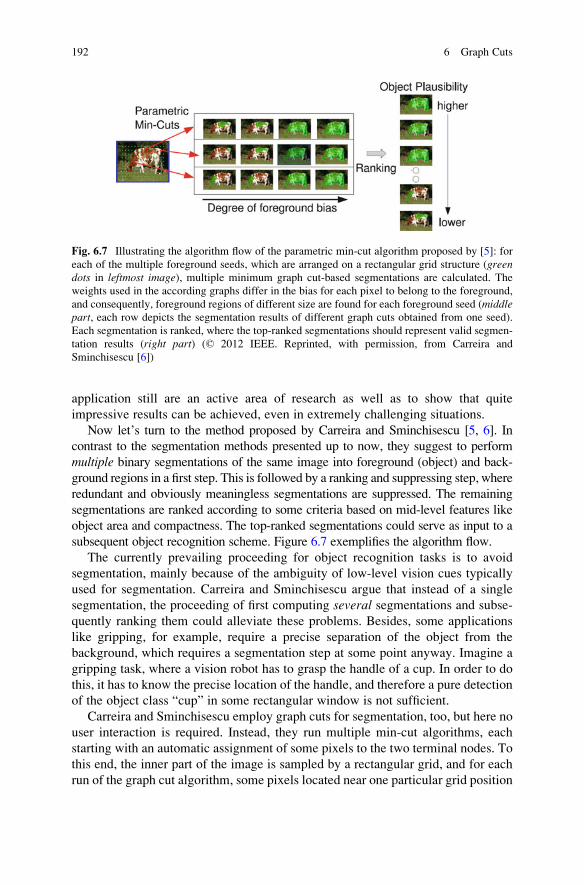
application still are an active area of research as well as to show that quite

impressive results can be achieved, even in extremely challenging situations.

Now let’s turn to the method proposed by Carreira and Sminchisescu [5, 6]. In

contrast to the segmentation methods presented up to now, they suggest to perform

multiple binary segmentations of the same image into foreground (object) and back-

ground regions in a first step. This is followed by a ranking and suppressing step, where

redundant and obviously meaningless segmentations are suppressed. The remaining

segmentations are ranked according to some criteria based on mid-level features like

object area and compactness. The top-ranked segmentations could serve as input to a

subsequent object recognition scheme. Figure 6.7 exemplifies the algorithm flow.

The currently prevailing proceeding for object recognition tasks is to avoid

segmentation, mainly because of the ambiguity of low-level vision cues typically

used for segmentation. Carreira and Sminchisescu argue that instead of a single

segmentation, the proceeding of first computing several segmentations and subse-

quently ranking them could alleviate these problems. Besides, some applications

like gripping, for example, require a precise separation of the object from the

background, which requires a segmentation step at some point anyway. Imagine a

gripping task, where a vision robot has to grasp the handle of a cup. In order to do

this, it has to know the precise location of the handle, and therefore a pure detection

of the object class “cup” in some rectangular window is not sufficient.

Carreira and Sminchisescu employ graph cuts for segmentation, too, but here no

user interaction is required. Instead, they run multiple min-cut algorithms, each

starting with an automatic assignment of some pixels to the two terminal nodes. To

this end, the inner part of the image is sampled by a rectangular grid, and for each

run of the graph cut algorithm, some pixels located near one particular grid position

Fig. 6.7 Illustrating the algorithm flow of the parametric min-cut algorithm proposed by [5]: for

each of the multiple foreground seeds, which are arranged on a rectangular grid structure (greendots in leftmost image), multiple minimum graph cut-based segmentations are calculated. The

weights used in the according graphs differ in the bias for each pixel to belong to the foreground,

and consequently, foreground regions of different size are found for each foreground seed (middlepart, each row depicts the segmentation results of different graph cuts obtained from one seed).

Each segmentation is ranked, where the top-ranked segmentations should represent valid segmen-

tation results (right part) (© 2012 IEEE. Reprinted, with permission, from Carreira and

Sminchisescu [6])

192 6 Graph Cuts

(the foreground seed) are linked to the foreground terminal. As far as the back-

ground terminal is concerned, some pixels of the image border are treated as

background seeds at each run.

Additionally, the cost function employed for the regional term features a param-

eter λ , whose value can be chosen arbitrarily. Different values of λ result in a

different bias of the cost function for assigning the pixels to the foreground.

Consequently, multiple segmentations can be produced with the same seed pixels,

as different values of λ are used. Please note that it is not necessary to run a separatemax-flow algorithm for each value of λ . Instead, a variant of the max-flow

algorithm, called parametric max flow, is able to calculate the minimum cuts for

all values of λ in a single run.

In a last step, the segmentations are ranked based on a vector of different region

properties like area, perimeter, and value of the cut (see [6] for details). As was

shown by the authors, the top-ranked segmentations allow for a plausible interpre-

tation of the scene, even in challenging situations. Their scheme performed best in

the VOC 2009 and VOC 2010 image segmentation and labeling challenges, which

supply a tough test bed and compare state-of-the-art algorithms. However, due to

the multiple runs of the min-cut algorithm, their method is rather slow.

Another recent approach using graph cuts in order to obtain a binary segmenta-

tion is presented by [15]. Within their method, the segmentation task is formulated

as the problem of finding the optimal boundary surrounding the region around a

so-called fixation point, which roughly speaking defines a point of special interest

which could be fixated by the eyes of a human observer. The fixation point can be

estimated automatically by evaluating the saliency of all pixels of the interest

region and taking the most salient one. This proceeding tries to imitate the human

visual system, where there is evidence that humans first fixate a characteristic point

and subsequently recognize the object around it.

Furthermore, the algorithm calculates a probability map being composed of the

probabilities of each pixel for being part of the region border. Various cues are

combined in order to estimate these probabilities. Obviously, intensity or color

discontinuities or changes in the texture around a pixel indicate a high probability of

being a border pixel. However, this can also occur inside an object.

In order to resolve this ambiguity, other cues like depth discontinuities (if a

stereo camera system is used) or motion (if a video sequence is available) can be

used (see [15] for details about how to combine the cues as well as the probability

map calculation). These so-called dynamic cues are much more unlikely to appear

in the interior of objects. For example, a sharp change of scene depth strongly

indicates that there is a transition form background to a foreground object being

located much closer to the camera at this position.

These probabilities are used for the boundary termBpq of (6.4) and the according

graph to be cut. This means that the weights of the n-links of pixels with high border

probability should be low. The Rp’s of (6.4) are chosen such that they represent all

knowledge about the segmentation before calculating the minimum graph cut.

More specifically, it can be assumed that the fixation point is part of the foreground,


whereas the image border pixels are part of the background. TheRp’s of those pixels

are set accordingly, whereas the Rp ’s of all other pixels are set to zero, as no

information about their bias is available. Now the graph is completely defined and

can be cut, e.g., via a max-flow algorithm.

As far as the shrinking bias is concerned, the authors of [15] try to avoid this

drawback by transforming the image into the polar space with equal spacing in the

annular as well as radial direction, where the fixation point coincides with the center

of the polar transform. Observe that circular contours of different diameter have

equal length in polar space. Therefore, it can be argued that the problem of graph

cuts tending to favor a segmentation of small regions with rather short boundaries

can effectively be suppressed by applying a polar transform and then building the

graph based on the polar space representation of the image, because then the

number of nodes to be severed is relatively independent of the region size.

The performance of the method is illustrated in Fig. 6.8. In the top row, three

challenging situations can be seen. The fixation point is marked by a green cross.

The images of the bottom row show the segmentation result (the segmented

foreground is highlighted and enclosed by a green contour). Despite significant

interior gradients, heavy background clutter, as well as objects featuring colors

similar to the background in some cases, the algorithm segments the object of

interest (almost) perfectly from the background.

6.1.5 Restriction of Energy Functions

This section deals with the following question: Which properties of a function are

necessary such that it can be minimized via graph cuts? This question is important,

because its answer can be used to guide the design of suitable energy functions as

Fig. 6.8 Demonstrating the performance of the algorithm proposed in [15]. See text for details (©2012 IEEE. Reprinted, with permission, from Mishra et al. [15])

194 6 Graph Cuts

well as to decide whether graph cuts can be employed for a given problem or not.

The paper of [14] investigates this issue and we will briefly mention the main

points here.

The energy function defined in (6.4) being used for segmentation is one example

of modeling a binary problem by a function which can be minimized by a graph cut

algorithm. A generalization of (6.4) can be written as

ð6:7Þ

where P denotes the image domain, lp defines some kind of binary assign-

ment to each pixel p (i.e., lp 2 0; 1½ �), Dp models the penalty of assigning label

lp to p, and Vpq models the cost of assigning lp to p and lq to q, with p and q being

adjacent pixels. Despite their compact and simple formulation, energy functions

in the form of (6.7) are hard to optimize, mainly because the dimensionality of

the space of unknowns is extremely large, as every pixel is treated as a separate

unknown. Hence, such problems often contain millions of unknowns. Conse-

quently, fast and efficient optimization algorithms are required (related to the

number of unknowns), and that’s where graph cuts come into play.

According to [14], energy functions of the type of (6.7) can be minimized via

graph cuts if the following condition holds:

Vpq 0; 0ð Þ þ Vpq 1; 1ð Þ � Vpq 0; 1ð Þ þ Vpq 1; 0ð Þ (6.8)

In other words, the sum of costs of assigning the same labels to p and q has to beat most equal to the sum of costs when p and q are assigned to opposite labels. Suchfunctions are said to be submodular. In the energy definition of (6.4), the δ-functionensures that the cost of assigning the same label to neighboring pixels is always

zero. Consequently, (6.8) holds if we assume nonnegative costs Vpq.

Informally speaking, the Dp ’s are data-driven cost terms and ensure that

the solution, i.e., the assigned labels, “fit well” to the observed data. The Vpq ’s

represent some prior information about the optimal solution. Because only neigh-

boring pixels are considered, the Vpq ’s essentially enforce spatial smoothness

by penalizing adjacent pixels with different labels.

This interpretation of (6.7) fits well into the demands of quite a variety of vision

applications including segmentation, object extraction, video texture synthesis, and

stereo reconstruction. Fortunately, the restrictions imposed by (6.8) are rather loose

and can be fulfilled in many cases as well. Together with the fact that graph cuts can

be extended to the multi-label case (which will be shown in the next sections), this

explains to a large extent why graph cuts have become increasingly popular among

the vision community over the last decade.


6.2 Extension to the Multi-label Case

With the graph cut methods presented up to now, only binary optimization

problems, which assign one out of two possible states to each pixel in an image

(or, more generally, voxel in a N-D data volume), can be solved. Because graph cut

optimization methods have the nice property of finding a global optimum, it is

desirable to extend the proceeding from the two-label case to the more general

multi-labeling problems, if possible.

In the multi-labeling problem, the task is to assign a label lp to each pixel p withlp 2 1; 2; . . . ; L½ �, i.e., each label can take one value out of a finite set of values withcardinality L . If we want to find an optimal labeling, the same kind of energy

function as in (6.7) can be applied, but now the lp’s (and lq’s) can take more than two

values.

As we will see below, there exist two ways in order to achieve this:

• Adaption of the topology of the graph: Essentially, each pixel is represented by

multiple nodes here. The number of nodes being necessary to represent one pixel

is in accord with the number of labels L: each pixel is represented by as many

nodes as are necessary such that one edge exists for each label. This means that

in order to get L edges, each pixel has to be represented by L� 1 nonterminal

nodes. This results in an extension of the graph to higher dimensions. When

calculating the minimum cut, it has to be ensured that exactly one of the edges

connecting the nodes belonging to the same pixel is severed by the minimum cut.

Now the severed edge uniquely identifies the value of the label of that pixel.

Observe that this proceeding is only applicable if the labels satisfy the so-called

linear ordering constraint (see below).

• Conversion into an iterative approximation scheme: Here, the multi-label prob-

lem is converted into a series of binary labeling problems, which are iteratively

solved and finally give an approximation of the multi-label solution. While an

exact calculation of the global solution typically is not possible, it can be shown

that the approximate solution lies within some constant factor of the “true”

global optimum. In other words, the approximate solution is sufficiently

“good” in many practical applications.

6.2.1 Exact Solution: Linearly Ordered Labeling Problems

A special case of multi-label problems is problems where the labels can be linearlyordered. Informally speaking, this means that considering any two labels a and b,there exists a measure which allows us to decide which of the two labels is smaller.

Moreover, we can assume that if a < b and b < c, a has to be smaller than c (a < c).Now we’re in the position to order all labels of the finite set in a linear ascending

order, i.e., a < b < c < . . . .

196 6 Graph Cuts

For example, consider the task of estimating disparities d in the two-camera

stereo matching problem, where we have to find a disparity d for each pixel. The

disparityd defines the position shift between a pixel in the left camera image and the

corresponding pixel in the image of the right camera, which depicts the same point

of the 3D scene being covered by the cameras. After a proper quantization of d, theproblem of identifying the (quantized) disparities for each pixel is a multi-labeling

problem where the labels (i.e., the quantized disparities) are linearly ordered. For

example, it is obvious that a disparity value of one pixel is smaller than a disparity

value of two pixels.

In contrast to that, consider a multi-label segmentation, where the image is

partitioned into multiple regions and each region is described by a unique label.

These labels cannot be linearly ordered, because it doesn’t make sense to define one

label as “smaller” than another.

6.2.1.1 Graph Construction

If a linear ordering of the labels is possible, we can give a natural definition of the

pairwise costsVpq, which depends on the difference between their labels lp and lq. In

the simplest case, Vpq can be set to the absolute differences lp � lq�� . Then, the

energy function can be written as

ð6:9Þ

where λpq is a weighting factor for setting the relative importance of the smoothness

term, which can be chosen differently for each pair of pixels, but is often set to a

constant: λpq λ 8 p; q.Without loss of generality, let’s further assume that the labels are integer values

in the range 1; 2; . . . ; L½ �. Then, the graph can be constructed as follows (see also

Fig. 6.9 for the simple illustrative case of only two pixels p and q). As usual, thegraph contains the two terminal vertices s and t. Additionally, L� 1 nodes p1; p2;. . . ; pL�1 are introduced for each pixel p.

These nodes are connected with the edges esp1 ; ep1p2 ; . . . ; epL�1t (black lines in

Fig. 6.9). Hence, there exist L such edges in the graph for each p and consequently,

each edge defines a (possible) labeling with one specific value. Therefore, let’s call

these edges “label edges.” The weights of those edges directly depend on the data-

driven costsDp, which specify the cost of applying a specific label to a node. We can

set wpl�1pl ¼ DpðlÞ þ Kp , where Kp is a constant (i.e., Kp takes identical values

for all edges relating to node p). The meaning of Kp will become clear later on.

Additionally, the graph also contains edges eplql connecting neighboring nodes

(cf. gray edges in Fig. 6.9. As we have only two pixels p and q, each node contains

only one of those edges for this example). Usually a 4-neighborhood is assumed.

The weight wplql of these edges should reflect the penalty when assigning different

labels to neighboring nodes. Therefore, these edges are also called “penalty edges.”

6.2 Extension to the Multi-label Case 197

The weight of those edges is set equal to the smoothness weighting factor: wplql

¼ λpq 8 l 2 1; 2; . . . ; L½ �. The reason for this will be clear soon.

A cut separating s from t (green line in Fig. 6.10) severs label edges as well as

penalty edges (dashed lines in Fig. 6.10). The severed label edges directly define the

labels assigned to each node. If, for example, the cut severs the edge ep1p2, the labellp ¼ 2 is assigned to pixel p. In the example of Fig. 6.10, based on the cut, we can

make the assignments lp ¼ 2 and lq ¼ 4.

Observe that the number of penalty edges of adjacent nodespandqbeing severedby the cut is equal to the absolute difference of the labels assigned to these nodes,

i.e., lp � lq�� . The sum of the weights of the severed edges should be equal to Vpq.

Considering the definition of Vpq in (6.9) (which is Vpq ¼ λpq � lp � lq�� ), this can be

achieved by setting the weight of each penalty edge wplql to λpq.If the cut shall uniquely define the labeling of each node (which is what we aim

for), it has to be ensured that it severs exactly one of the label edges belonging to

one node, i.e., the graph must not contain “folds.” This can be enforced by an

appropriate choice of Kp: if the Kp’s are sufficiently large, a cut severing multiple

label ledges belonging to the same pixel will become too costly. Therefore, theKp is

set slightly larger than the sum of the weights of all penalty edges belonging to pixel

where defines the neighborhood of p. As the same Kp

is added to all label edges relating to node p, the relative influence of the Dp lp� �

is

not affected by the introduction of the Kp.

Please note that the property of finding the global optimum can only be assured

through the special design of the Vpq term of the energy function, which takes the

L1 norm.

On the other hand, however, the L1 norm might tend to produce oversmoothing

in the vicinity of sharp boundaries in the data (e.g., large jumps of disparity in stereo

matching), because large jumps between adjacent pixels lead to a costly cut

Fig. 6.9 Exemplifying the graph construction for multi-label problems with just two pixels pand q; where each pixel is related to the black nodes of one row of the graph. The terminal

nodes are indicated by red and blue color

Fig. 6.10 Illustrating how a cut (green) helps identifying the label assignment

198 6 Graph Cuts

severing many penalty edges. Consequently, the optimization intends to minimize

the number of pixels where such a large jump occurs and therefore irregularly

shaped object boundaries tend to be smoothed. This behavior could be improved by

truncating the L1 norm, but truncated L1 norms cannot be represented by the graph

topology introduced in this section. Truncated, discontinuity-preserving energy

functions can be treated by the approximation methods presented in Sect. 6.2.2.

6.2.1.2 Example: Stereo Matching

Graphs with a topology just described are suitable for usage in stereo matching (see

[17, 18]). Consider the standard two-camera stereo setup, where the same scene is

captured by two spatially separated cameras, whose optical axes are parallel, i.e.,

they have the same viewing direction. Due to the displacement between the two

cameras, the same scene position is depicted with a slight shift when we compare

the images acquired by the two cameras. This shift is called disparity d.The disparity d directly relates to the geometry of the setup of the two cameras.

In the standard setup, the cameras are shifted only horizontally, i.e., the line

connecting the two camera centers (also called baseline) is parallel to the x-axis.

As a result, the positions in the two camera images depicting the same scene point

also feature a horizontal shift, i.e., I1 x; yð Þ ¼ I2 x� d; yð Þ.If we know the disparityd as well as some camera calibration parameters, we can

infer the depth of the scene position from the tuple x; y; d½ � . Therefore, the task

of stereo matching results in identifying the disparityd for each x; y½ �-position of oneof the two camera images. Without loss of generality we further assume that I1 is

acquired by the left of the two cameras. As a consequence, d is always nonnegative.As we know that pixels depicting the same scene point must be located upon

straight lines (which are called epipolar lines), it is sufficient to perform indepen-

dent searches along these epipolar lines (which are horizontal lines in our case), i.e.,

jointly estimate the disparity for one row of the image in a separate step and then

move on to the next row. The optimization of each row can be solved efficiently

with a dynamic programming approach, for example.

However, the independent optimization leads to artifacts, because the disparity

usually tends to be smooth in both directions in the image plane. This effect can be

tackled by a post-processing of the calculated disparities after estimating them for

each row independently. It would be more convenient though to perform a global

optimization of the entire image plane, which could incorporate smoothness

constraints in both directions (x and y) in a natural way.

This can be achieved by the usage of graph cuts adapted for multi-labeling

problems as presented in the previous section. In order to apply graph cuts, we have

to quantize and constrain the search space such that the searched disparities can be

expressed by a finite set of integer values: d 2 0; 1; . . . ; dmax½ � . In [17], it is

suggested to construct the graph as follows (see also Fig. 6.11):

Each pixel p is represented by dmax þ 2 nodes in the d-direction, which are

connected by label edges as described in the previous section. Consequently, there


exist dmax þ 1 label edges for each pixel p , and each label edge represents one

disparity of the set 0; 1; . . . ; dmax½ �. In order to catch the whole image, there exist

W � H nodes at each disparity level (whereW andH denote the image dimensions).

All “front” nodes p0 are connected to the source s of the graph, whereas all “back”nodes pdmaxþ1 are connected to the sink t. Adjacent nodes of the same disparity level

(which are of equal d value) are connected by penalty edges. As can be seen in

Fig. 6.11, a 4-neighborhood is assumed (cf. the encircled close-up).

A cut through this graph separating s from t can be interpreted as a hyperplane

separating the matching volume. The label edges severed by the cut define the

disparities as follows: if edge epdpdþ1 is severed by the cut, then the disparity d is

assigned to pixel p.Concerning the edge weights, the weights of all t-links connecting s or t to some

other node are set to infinity. This ensures that these edges are never severed by the

minimum cut. The weight of all penalty edges is set to a constant K , which is a

smoothness factor. If K ¼ 0, there is no penalty even for large disparity jumps

between adjacent pixels. On the other hand, a value of K ¼ 1 would enforce that

no penalty edge is severed at all by the minimum cut, and consequently all pixels

would be assigned to the same disparity. Reasonable values of K are in between

these two extremes and should lead to a well-balanced trade-off between data

fidelity and smoothness.

The weight of the label edges should reflect the suitability of a given disparity to

explain the data. If the assumption that we have a certain disparity d at pixel p¼ x; y½ � is correct, the intensity I1 x; yð Þobserved in the first camera image at position

x; y½ � should be very similar to the intensity I2 x� d; yð Þ of the second camera image

observed at position x� d; y½ �, because both pixels depict the same scene object.

front

Back

Sink

Ta

Source

S

b

d

Cut(depth surface)

Fig. 6.11 Depicting the graph topology utilized in [17] for stereo matching. Please note that the

axes denoted as a and b correspond to x and y, which is the notation used in the text (From Roy

[17], with kind permission from Springer Science and Business Media)

200 6 Graph Cuts

Consequently, the weight wpdpdþ1 can be set to the L2 norm of the intensity

difference between corresponding pixels in both camera images:

wpdpdþ1 ¼ I1 x; yð Þ � I2 x� d; yð Þ½ �2 þ C (6.10)

where C is a constant which is chosen sufficiently large enough in order to ensure

that exactly one label edge is cut for each pixel (and thus prohibits folds of the cut).

If the intensity difference between I1 x; yð Þ and I2 xþ d; yð Þ is low, this indicates thatthe corresponding disparity is a good solution and consequently wpdpdþ1 is low.

Now the graph is completely defined. As it is a two-terminal graph, the minimum

cut can be calculated with any max-flow method, such as the augmenting path

algorithm presented in Sect. 6.1.2.

An example of the performance of the method can be seen in Fig. 6.12, which

shows a pair of stereo images depicting a house wall with some shrubs and a sign

placed in front of it (first row). The second row shows disparity maps calculated by

various methods. The left map is calculated by a standard dynamic programming

approach, which performs separate optimizations for each row. The artifacts in the

vertical direction introduced by separately optimizing disparities for each row are

clearly visible. Post-processing (middle map, histogram equalized) improves the

situation but cannot eliminate the artifacts completely. The usage of the max-flow

graph cut method presented in this chapter (right map), however, clearly gives the best

Fig. 6.12 Illustrating the performance of graph cuts used in stereo matching. The top row shows a

pair of stereo images, whereas the bottom row shows the solutions obtained with the standard DP

approach of stereo matching (left), DP with post-processing (middle), and graph cuts (right) (FromRoy [17], with kind permission from Springer Science and Business Media)


results, as disparities are smoothed in both directions such that a global optimum of the

underlying energy function is found. Please note, however, that dynamic programming

approaches typically are significantly faster than the max-flow method used here.

This indicates that the quality of the solution can significantly be improved by

the spatial smoothing introduced with the weights of the penalty edges, which is set

to K. The influence of different choices of K is visualized in Fig. 6.13 (also for the

shrub example depicted in the top row of Fig. 6.12). Whereas not considering any

smoothing at all (K ¼ 0) produces very noisy results of poor quality, it can be seen

that a fairly wide range of smoothing parameters lead to good results (middle

images). Of course, very high smoothing parameters lead to oversmoothed results

(right image).

6.2.2 Iterative Approximation Solutions

One drawback of the exact solution of the multi-labeling problem presented in the

previous section is that it requires non-discontinuity-preserving interaction

potentials such as Vpq / lp � lq�� . However, such functions tend to oversmoothing,

becauseVpq is not bounded and can get very large at discontinuities where the labels

lp and lq differ significantly between adjacent pixels p and q (which will occur at

some position in most images). Consequently, the algorithm tends to avoid large

discontinuities by reducing the number of pixels they occur at as much as possible.

A possible solution is to bound the cost of assigning different labels, such as

Vpq ¼ λpq �min lp � lq�� ;K� �

, where λpq � K is the upper bound. Now, large

discontinuities don’t lead to increased costs any longer and therefore are chosen

with higher probability by the optimization algorithm. A special case is the simplest

of such bounded functions, the so-called Potts model, where all different labelings

between adjacent pixels are punished by the same cost:

Vpq ¼ λpq � T lp 6¼ lq� �

with T ¼ 0 if lp ¼ lq1 if lp 6¼ lq

�(6.11)

Fig. 6.13 Depicting the role of the smoothing parameter K of the min-cut method for the stereo

image pair presented in Fig. 6.12 (From Roy [17], with kind permission from Springer Science and

Business Media)

202 6 Graph Cuts

Observe that the Potts model can also be used for problems where the values of

the unknowns cannot be linearly ordered. Imagine a segmentation problem where

the task is to partition the image into multiple regions. Setting the interaction

potentials according to (6.11) allows to equally punish all positions where the labels

of adjacent pixels are different, regardless of the actual values.

Such bounded functions, however, don’t allow for a global minimum cut

solution, even for the simplest case of the Potts model. Therefore, Boykov et al.

[4] suggested an iterative scheme, which approximates the solution. They also

showed that the approximate solution lies within a small multiplicative constant

of the global optimum, which makes the method interesting for practical use.

At each iteration, the authors of [4] propose to solve a binary decision problem,

which can be modeled by a two-terminal graph we are already familiarized with.

Hence, each of those binary problems can be solved by the min-cut/max-flow

algorithm already presented.

Iterative algorithms for that type of energy minimization problems were already

used before graph cuts emerged. A formerly quite commonly used algorithm is the

so-called simulated annealing method (see, e.g., Chap. 2 or [10]). However, many

of those algorithms performed what the authors of [4] call a “standard move” at

each iteration. Within a standard move, the labeling of just one single pixel isallowed to change. As a consequence, a very large number of iterations have to be

performed until the solution is finally found.

In order to overcome this drawback, Boykov et al. proposed to perform the

so-called large moves. During execution of each large move, the labeling of manypixels is allowed to change in a single iteration. They suggested two types of such

moves, namely, expansion moves and swap moves (see also Fig. 6.14).

During one swap move, all pixels with current labelα are allowed to change theirlabel to β, and, respectively, all pixels with current label β are allowed to change

their label to α, if this reduces the total cost. All pixels labeled different from α or βhave to keep their label (see (c) in Fig. 6.14, where the transition between the red

and blue areas in the lower part of the image is rectified).

Fig. 6.14 Illustrating different single moves of an iterative approximation. Suppose an initial

labeling consisting of three labels α, β , and γ (a). In a standard move, which is used by many

iterative optimization schemes, the label of only one pixel is allowed to change during a single

iteration (highlighted by a white circle in (b)). An α� β � swap move (c) allows all pixels withcurrent labelαorβ to swap their label. An expansion move (d) allows the expansion of the labelα tomany pixels with a previous labeling different from α at once. As clearly can be seen, both move

types allow for significant changes in a single step


http://dx.doi.org/10.1007/978-1-4471-5283-5_2

In one α� expansion move, the label α is allowed to “expand,” i.e., the label of

all pixels with current labeling different from α is allowed to be changed to α if thisimproves the situation. Moreover, all pixels with current labelαmaintain their label

(see (d) in Fig. 6.14, where the red area of all pixels labeled α is expanded).

The possibility to change the labels of many pixels simultaneously in one

iteration step significantly accelerates the optimization, which is quite obvious if

we compare the labeling changes of (c) or (d) with (b) in Fig. 6.14.

An important observation is that the decision which label has to be assigned to

each pixel during one expansion move or swap move essentially is a binary

decision. Due to the nature of the large moves, the pixels either keep their labels

or change it, but there is only one value to which the labels can switch. In α�expansion moves, for example, all pixels labeled different from α can either keep

their current label or change it to α. Similarly, all pixels labeled α (or β) can either

keep their label or change it to β (or α, respectively) in one swap move.

These binary decisions are well suited for being represented by a two-terminal

graph, which reveals the optimal decision through the calculation of its minimum

cut. Observe that in contrast to the examples of Sect. 6.1, the topology of the graphs

involved here depends on the current labeling, and, consequently, a different graph

has to be built at each iteration.

As far as the overall proceeding when expansion moves are employed is

concerned, we can iterate through the set of all possible labels 1; 2; . . . ; L½ � , bybeginning with an α� expansion move with α ¼ 1 (i.e., solve this binary decision

problem by calculating the min-cut/max-flow of the according graph), then con-

tinue to do the same with α ¼ 2, and so on, until α ¼ L is reached. This is what is

called a “cycle” in [4]. Consequently, a cycle consists ofOðLÞ single moves. If any

of these L expansion moves was able to make any progress, i.e., could achieve a

reduction of the overall cost, the system performs another cycle, and so on, until

none of the expansion moves of the cycle was able to reduce the total cost (see also

the flowchart of Fig. 6.15). Similarly, one cycle of α� β � swap moves consists of

finding a minimum graph cut for every combination of α and β labels.

6.2.2.1 Graph Cut Optimization with Swap Moves

If swap moves are to be utilized, we have to perform an α� β � swap move for all

possible combinations of α and β in each cycle with the only restriction that it

suffices to consider only combinations where α < β. This is because Vpq has to be

symmetric, as we will see later. Therefore, combinations withα > β can be omitted.

Furthermore, swapping doesn’t make sense if α ¼ β. Hence, each cycle contains

O L2ð Þ single moves when α� β � swap moves are carried out.

Now let’s turn to the question how to build the graph for solving the binary

decision problem of each single move. For swap moves, we just have to include all

pixels into the graph whose current label is α or β, because the label of all other

nodes/pixels must not change and therefore these pixels don’t need to be

204 6 Graph Cuts

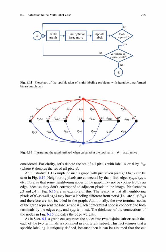
considered. For clarity, let’s denote the set of all pixels with label α or β by Pαβ

(where P denotes the set of all pixels).

An illustrative 1D example of such a graph with just seven pixels p1 to p7 can beseen in Fig. 6.16. Neighboring pixels are connected by the n-link edges ep1p2, ep2p3,etc. Observe that some neighboring nodes in the graph may not be connected by an

edge, because they don’t correspond to adjacent pixels in the image. Pixels/nodes

p3 and p4 in Fig. 6.16 are an example of this. The reason is that all neighboring

pixels of p3 as well as p4may have a labeling different from α or β (i.e., are all =2Pαβ)

and therefore are not included in the graph. Additionally, the two terminal nodes

of the graph represent the labelsαandβ. Each nonterminal node is connected to both

terminals by the edges ep3α and ep3β (t-links). The thickness of the connections ofthe nodes in Fig. 6.16 indicates the edge weights.

As in Sect. 6.1, a graph cut separates the nodes into two disjoint subsets such that

each of the two terminals is contained in a different subset. This fact ensures that a

specific labeling is uniquely defined, because then it can be assumed that the cut

S

E

Buildgraph

Find optimallarge move

Cyclecompleted ?

yes

no

Updatelabels

E reduced incurrent cycle ?

no

yes

Fig. 6.15 Flowchart of the optimization of multi-labeling problems with iteratively performed

binary graph cuts

Fig. 6.16 Illustrating the graph utilized when calculating the optimal α� β � swap move


severs exactly one t-link of each nonterminal node. In contrast to the examples of

Sect. 6.1, however, here a node is assigned to the label whose corresponding edge is

actually severed. For example, if the cut severs ep1β, the pixel p1 is assigned to labelβ. This can be ensured by a proper choice of the edge weights.

Moreover, the weights have to be chosen such that the minimum cut defines a

labeling of all pixels p 2 Pαβ which reduces the cost function as much as possible.

This is in fact just a local minimum of the total cost, because the labeling of all other

pixels is enforced to remain constant during one α� β � swap move and therefore

the global optimum is not reached. We can set the weightswpq of the n-links to Vpq,

because if a cut severs neighboring nodes, this means that one pixel is assigned to

label α and the other to β and, according to the definition of the cost function (6.7),

this assignment should be punished by the quantity Vpq α; βð Þ.As far as the weights of the t-links are concerned, they are set according to

ð6:12Þ

Clearly, these weights should contain the data termDp. Additionally, some costs

for all pixels adjacent to p with a labeling different from α or β (i.e., )

have to be included. The reason for this is that the interaction costs of the pixel pairs

consisting of p and one of those pixels are not considered in the current graph so far,simply because those pixels are not included in the current graph. Therefore, these

costs should be added to the according t-link cost.

If we assign the labelα to p, for example, this induces pairwise costs for all pixels

q adjacent to p with a labeling different from α (i.e., lq 6¼ α). Some of those pixels

already are included in the current graph (namely, the ones with label β ), and,consequently, their pairwise cost is considered by the weight of the n-link linking

both nodes. However, all neighbors of pwhich are not contained in Pαβ are missing

in the current graph and therefore these pairwise costs are added to wpα . Similar

considerations can be made for the wpβ.

Now the graph is completely defined, the minimum cut can be efficiently

obtained by a max-flow algorithm, such as the one presented in Sect. 6.1.

As α� β � swap moves work with undirected graphs with positive edge

weights, we have to constrain the pairwise costs such that they are symmetric and

nonnegative, i.e., Vpq α; βð Þ ¼ Vpq β; αð Þ 0. Furthermore, the Vpq is set to zero

where the neighbors p and q are assigned the same value: Vpq α; αð Þ ¼ 0. Any

function Vpq satisfying these two conditions is said to be a semi-metric. Hence, α�β � swap moves are applicable if Vpq is a semi-metric.

Pseudocode

function multiLabelOptSwap (in image I, in data-driven costfunction Dp, in pairwise cost function Vpq, in initial label-

ing l0 (arbitrary), out optimized labeling l�)

k 0

// main iteration loop (one pass is one cycle)

206 6 Graph Cuts

repeat// loop for all swap moves within one cycle (allcombinations of α and β)bSuccess false // flag indicating whether reduction of

total cost was possible in current cyclefor α ¼ 1 to L

for β ¼ αþ 1 to L// construction of graph G ¼ N;Eð ÞN sα; tβ

� // add the two terminals

for all pixels p 2 Pif p 2 Pαβ then // label of p is either α or β

N N [ pf g // add p to node set

E E [ epα; epβ�

// connect p to src and sink

set wpα and wpβ according to (6.12)end if

nextfor all neighboring pixels p 2 Pαβ and q 2 Pαβ

E E [ epq�

, wpq Vpq α; βð Þnext// find optimal α� β � swap movecalculate minimum cut C� of Gfor all pixels p 2 Pαβ

if epα 2 C� thenlkþ1p α // assign label α to pixel p

else

lkþ1p β // assign label β to pixel p

end ifnext// check convergence

if E lkþ1� �

< E lk� �

then

bSuccess true // total energy could be reducedend if

nextnextk k þ 1

until bSuccess ¼¼ false

// set solution to current labeling

l� lk

6.2.2.2 Graph Cut Optimization with Expansion Moves

The other possibility of approximating multi-label optimization by iteratively

solving binary problems suggested in [4] is to perform α� expansion moves,


where the label α is allowed to “expand,” i.e., any pixel currently labeled different

fromα is allowed to change its label toα at each iteration, whereas all pixels alreadylabeled α keep their label. As with swap moves, the optimal α� expansion move

can also be found by the construction of an appropriate two-terminal graph,

followed by the calculation of the minimum cut of this graph as follows.

The two terminals of this graph represent the labelsα and �α (see Fig. 6.17). Pixelsassociated to the �α-terminal keep their current labels, which are different from α.Like with expansion moves, all edges severed by a cut indicate to which terminal a

particular node/pixelpbelongs: If edge epα is severed by the cut, the label ofp isα ; ifep�α is severed, p keeps its current label lp, which is different from α.

Because every pixel of an image is labeled either to α or to �α , all pixels areincluded in the graph here. Every node is connected to both terminals by the edgesepαand ep�α , where the weight wpα is set to the data-driven cost of assigning α to p:wpα ¼ Dp αð Þ . As far as the weights wp�α are concerned, we have to distinguish

whether the current label of p is α or not. Because the region of pixels labeled α can

be expanded only, we have to ensure that no node with current label α is assigned

to the�α-terminal by the cut. This can be done by settingwp�α ¼ 1 for all pixelsp 2 Pα

(p1 in Fig. 6.17). For all other nodes p =2 Pα; we can set wp�α ¼ Dp lp� �

, where lpdenotes the current label of p.

As far as the n-links are concerned, there is a fundamental difference between

neighbors p and qwhich are assigned to the same label and neighbors with different

labeling.

If p and q share the same label lp, an assignment of one of them to α and the otherto �αmeans that the cut must sever the n-link epq between them. Because both nodes

previously had the same label, the cost wpq for this assignment can be set to Vpq

lp; α� �

, regardless of whether p or q is now assigned to α.Obviously, for pairs p and qwith different labels (lp 6¼ lq), this does not work any

longer. Here, the costs are different depending on whether p or q is assigned to α

Fig. 6.17 Illustrating the graph utilized when calculating the optimal α� expansion move, where

p1 is currently assigned to α, p2, p3, and p4 are all assigned to some other label β, whereas p5 is

assigned to label γ

208 6 Graph Cuts

after the current move (i.e., Vpq lp; α� �

or Vpq lq; α� �

). This can be resolved by the

introduction of an auxiliary nodea, which is placed in betweenpandq (there are twoexamples of such auxiliary nodes in Fig. 6.17, which are shown in green, as lp1 6¼ lp2and lp4 6¼ lp5). Now we have two n-links epa and eaq, where we can define the weights

wpa ¼ Vpq lp; α� �

and waq ¼ Vpq α; lq� �

. Now the costs of both possibilities are

modeled in the graph.

But how to connect the auxiliary node to the terminals and how to choose the

weights for those links? Figure 6.18, where a part of the graph containing an

auxiliary node a is shown, helps to explain the choice. First, we note that a is

only connected to the �α-terminal. Then, there exist two possible ways of a cut which

assigns p to �α and q to α (left and right part of Fig. 6.18, cut in green). Both possiblecuts sever edges ep�α and eαq (indicated by dotted edges), but the cut on the left

additionally severs epa, whereas the cut on the right severs eaα and eaq.Obviously, the left cut is “correct,” because it correctly accounts for the pairwise

cost Vpq lp; α� �

to be considered as p is assigned to �α (i.e., keeps its current label lp)

and q is labeled withα. An appropriate choicewa�α should make sure that the graph is

always cut in this way. When we setwa�α ¼ Vpq lp; lq� �

, it can be enforced that the cut

severs epa if we impose additional constraints on the pairwise cost function. More

specifically, the so-called triangle inequality has to hold:

Vpq lp; α� � � Vpq lp; lq

� �þ Vpq lq; α� �

(6.13)

Additionally, Vpq has to be nonnegative and symmetric as well, because it has to

be ensured that Vpq lp; lp� � ¼ 0, which are the same constraints as with swap moves.

All conditions are fulfilled if Vpq is a (true) metric. For example, the Potts model

(6.11) meets all of these conditions.

Fig. 6.18 Exemplifying the two possibilities of a cut when p and q are assigned to different labels(cut in bold green)


Observe that the constraints for swap moves are not as restrictive as for expan-

sion moves (no triangle inequality required), which makes swap moves applicable

to a broader range of applications. In terms of runtime, however, expansion moves

typically converge faster, mainly because each cycle contains less single moves.

This overcompensates the effect that each single move has a higher complexity

compared to swap moves.

Pseudocode

function multiLabelOptExpansion (in image I, in data-drivencost function Dp, in pairwise cost function Vpq, in initial

labeling l0 (arbitrary), out optimized labeling l�)

k 0

// main iteration loop (one pass is one cycle)repeat

bSuccess false // flag indicating whether reduction oftotal cost was possible in current cycle

// loop for all expansion moves within one cyclefor α ¼ 1 to L

// construction of graph G ¼ N;Eð Þcreate one node for each pixelN N [ sα; t�αf g // add the two terminals// add t-links to both terminals for each node/pixelfor all pixels p 2 P

E E [ epα; ep�α�

set t-link weights appropriatelynextfor all neighboring pixels p and q

if lkp 6¼ lkq then // p and q have different labels

N N [ af g // add an auxiliary node a

E E [ epa; eaq; ea�α�

// connect a to p, q and sink

wa�α Vpq lkp; lkq

�, wpa Vpq lkp; α

�, waq Vpq α; lkq

�

else // p and q have the same label

E E [ epq�

, wpq Vpq lkp; α �

end ifnext// find optimal α� expansion movecalculate minimum cut C� of Gfor all pixels p 2 P

if epα 2 C� thenlkþ1p α // assign label α to pixel p

else

lkþ1p lkp // keep current labeling for p

210 6 Graph Cuts

end ifnext// check convergence

if E lkþ1� �

< E lk� �

then

bSuccess true // total energy could be reducedend if

nextk k þ 1

until bSuccess ¼¼ false

// set solution to current labeling

l� lk

6.2.2.3 Example: Nonrigid Cat Motion

Boykov et al. tested the performance of their algorithm in various applications. One

of them, namely, a motion prediction (aka optical flow), is presented here. Taking a

pair of images depicting the same scene at different times, the task is to predict for

each scene element how much it has moved within the period of time between both

image acquisitions, i.e., to calculate the disparity between a pixel showing the same

scene element.

Because motion is two-dimensional, we have a vertical as well as a horizontal

displacement. Two-dimensional disparity can be modeled by a labeling such that

the label of a pixelpconsists of two components: lhp indicating horizontal motion and

lvp indicating vertical motion, respectively. As graph cuts only work with scalars,

every combination of lhp and lvp can be represented by a scalar number lp. In [4], eight

horizontal and five vertical displacements are used; hence, this amounts to 40 labels

altogether.

As with stereo, the displacements attributed to adjacent pixels should be similar

for most positions. However, usually discontinuities occur at the borders of moving

objects. Therefore, the pairwise cost Vpq lp; lq� �

is set to the truncated measure Vpq

lp; lq� � ¼ K �min 8; lhp � lhq

�2þ lvp � lvq

�2� . Because this measure doesn’t fulfill

the triangle inequality, the swap algorithm is used for optimization.

Figure 6.19 shows an example of a cat moving in front of a highly textured

background (a). Despite texture helps to calculate a dense motion field, its calcula-

tion still is a difficult task as the cat’s motion is nonrigid. The horizontal movement

result is shown in (b) and vertical movement in (c) (gray coded). As can be seen,

the cat is clearly separated from the background and was accurately detected by the

algorithm. The running time reported in [4] has to be seen in the context of the

hardware available at reporting date and should be in the order of seconds for

images of several 100,000 s of pixels with up-to-date hardware.


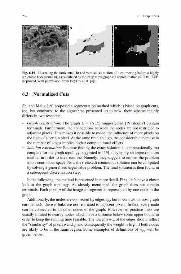
6.3 Normalized Cuts

Shi and Malik [19] proposed a segmentation method which is based on graph cuts,

too, but compared to the algorithms presented up to now, their scheme mainly

differs in two respects:

• Graph construction: The graph G ¼ N;Eð Þ suggested in [19] doesn’t contain

terminals. Furthermore, the connections between the nodes are not restricted to

adjacent pixels. This makes it possible to model the influence of more pixels on

the state of a certain pixel. At the same time, though, the considerable increase in

the number of edges implies higher computational efforts.

• Solution calculation: Because finding the exact solution is computationally too

complex for the graph topology suggested in [19], they apply an approximation

method in order to save runtime. Namely, they suggest to embed the problem

into a continuous space. Now the (relaxed) continuous solution can be computed

by solving a generalized eigenvalue problem. The final solution is then found in

a subsequent discretization step.

In the following, the method is presented in more detail. First, let’s have a closer

look at the graph topology. As already mentioned, the graph does not contain

terminals. Each pixel p of the image to segment is represented by one node in the

graph.

Additionally, the nodes are connected by edges epq, but in contrast to most graph

cut methods, these n-links are not restricted to adjacent pixels. In fact, every node

can be connected to all other nodes of the graph. However, in practice links are

usually limited to nearby nodes which have a distance below some upper bound in

order to keep the running time feasible. The weights wpq of the edges should reflect

the “similarity” of pixels p and q, and consequently the weight is high if both nodesare likely to be in the same region. Some examples of definitions of wpq will be

given below.

Fig. 6.19 Illustrating the horizontal (b) and vertical (c) motion of a cat moving before a highly

structured background (a) as calculated by the swap move graph cut approximation (© 2001 IEEE.

Reprinted, with permission, from Boykov et al. [4])

212 6 Graph Cuts

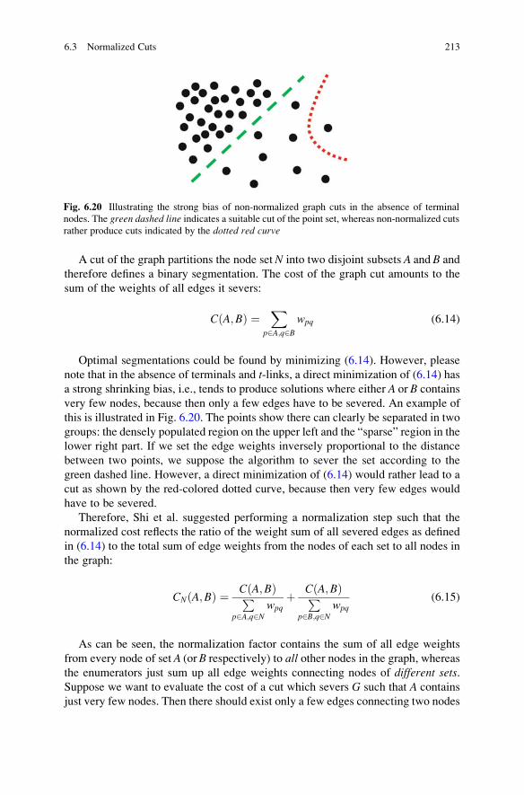
A cut of the graph partitions the node set N into two disjoint subsets A and B and

therefore defines a binary segmentation. The cost of the graph cut amounts to the

sum of the weights of all edges it severs:

C A;Bð Þ ¼X

p2A;q2Bwpq (6.14)

Optimal segmentations could be found by minimizing (6.14). However, please

note that in the absence of terminals and t-links, a direct minimization of (6.14) has

a strong shrinking bias, i.e., tends to produce solutions where either A or B contains

very few nodes, because then only a few edges have to be severed. An example of

this is illustrated in Fig. 6.20. The points show there can clearly be separated in two

groups: the densely populated region on the upper left and the “sparse” region in the

lower right part. If we set the edge weights inversely proportional to the distance

between two points, we suppose the algorithm to sever the set according to the

green dashed line. However, a direct minimization of (6.14) would rather lead to a

cut as shown by the red-colored dotted curve, because then very few edges would

have to be severed.

Therefore, Shi et al. suggested performing a normalization step such that the

normalized cost reflects the ratio of the weight sum of all severed edges as defined

in (6.14) to the total sum of edge weights from the nodes of each set to all nodes in

the graph:

CN A;Bð Þ ¼ C A;Bð ÞPp2A;q2N

wpqþ C A;Bð ÞP

p2B;q2Nwpq

(6.15)

As can be seen, the normalization factor contains the sum of all edge weights

from every node of set A (or B respectively) to all other nodes in the graph, whereasthe enumerators just sum up all edge weights connecting nodes of different sets.Suppose we want to evaluate the cost of a cut which severs G such that A contains

just very few nodes. Then there should exist only a few edges connecting two nodes

Fig. 6.20 Illustrating the strong bias of non-normalized graph cuts in the absence of terminal

nodes. The green dashed line indicates a suitable cut of the point set, whereas non-normalized cuts

rather produce cuts indicated by the dotted red curve

6.3 Normalized Cuts 213

which are both elements ofA. Consequently, a large fraction of all edges connectinga node of A to some other node is severed by the cut (as there should be more edges

epq connecting p 2 A to some node q 2 B than edges connecting p 2 A to q 2 A).As a result, the first summand of (6.15) should be near 1 and therefore the relative

cost of such a cut should be high compared to other cuts.

Now, we are interested how to find a cut which minimizes (6.15). Assume that

the binary segmentation is indicated by a vector x of dimensionality n (where ndenotes the number of pixels), whose elements can take two values. If xp ¼ 1, then

p is assigned to A, whereas a value of xp ¼ �1 indicates that p 2 B. Moreover, the

total sum of the weights of all edges containing p is denoted by dp ¼Pqwpq. Now

we can rewrite the cut cost in terms of x and the dp ’s. In order to find a proper

segmentation, we have to minimize the following expression:

x� ¼ argminx

CN xð Þ ¼ argminx

Pxp>0; xq<0

�wpqxpxq

Pxp>0 dp

þ

Pxp<0; xq>0

�wpqxpxq

Pxp<0 dp

(6.16)

However, it turns out that finding the exact solution x� is NP-complete

and therefore infeasible, because typically n can amount up to hundreds of

thousands or even millions. Therefore, Shi et al. suggest calculating an approxi-

mate solution. LetD be a diagonal matrix of dimensionality n� n, whose diagonalelements are set to the dp ’s and W denote the n� n matrix with its elements

equal to the edge weights, i.e., W p; qð Þ ¼ wpq. Together with the introduction of

k ¼Pxp>0 dpP

p dp

., b ¼ k

1�k , and y ¼ 1þ xð Þ � b 1� xð Þ, the authors of [19]

showed that a minimization of (6.16) is equal to the following relation:

y� ¼ argminx

CN xð Þ ¼ argminy

yT D�Wð ÞyyTDy

(6.17)

where the elements ofycan take the binary values �b; 1f g, i.e.,yp 2 �b; 1f g. Pleaseobserve that the right part of (6.17) is the well-known Rayleigh quotient. If we relaxthe binary constraint and allow the yp to take real values (i.e., embed the problem in

a continuous space), then we can make use of the fact that the Rayleigh quotient can

be minimized by calculating the eigenvectors of the generalized eigensystem

D�Wð Þy ¼ λDy (see, e.g., [12]). In other words, Shi et al. transform the original

problem to a more convenient representation (we now seek an indicator vector yinstead of x) and then employ a continuous spectral (i.e., eigenvalue) method to

obtain the graph cut (which is discrete by nature). Of course, this is totally different

to the discrete methods described up to now in this chapter.

For the relaxed continuous problem, there exist n generalized eigenvectors vi ,which can be sorted according to their eigenvalues λi. Please note that there alwaysexists the trivial solution λ1 ¼ 0, v1 ¼ 1, because by definition dp is the sum of all

edge weights associated with node p, which are exactly the elements of the pth row

214 6 Graph Cuts

ofW. Without going into details, a property of the Rayleigh quotient is that we can

obtain our solution by taking the eigenvector v2 associated to the second smallest

eigenvalue (see [12]): y� ¼ v2.Becausev2 is real-valued, we have to threshold its elements in order to determine

the segmentation, i.e., transform the solution back to the discrete domain. To this

end, various simple methods exist, e.g., a simple thresholding operation, where the

pixels corresponding to all elements above the threshold t are assigned to one node

set and the pixels corresponding to all elements below t are assigned to the other

node set, respectively. As far as the choice of t is concerned, it can, e.g., be set to themedian of the elements of v2.

Overall, the algorithm comprises the following steps (see also flowchart of

Fig. 6.21):

1. Graph construction: Given an image I, build the graphG ¼ N;Eð Þ such that anypixel p is represented by one node and is connected to the other nodes accordingto the weightswpq (examples of a proper choice of the weighs will follow below).

2. Rayleigh quotient formulation: Derive D and W from the edge weights.

3. Spectral solution: Calculate the eigenvalues of the generalized eigenvalue

system D�Wð Þy ¼ λDy.4. Binary decision: Take the second smallest eigenvector v2 and perform a binary

partitioning of the image according to the values of the elements of v2 (above orbelow threshold t).

The suitability of the spectral solution of the normalized cut is illustrated in

Fig. 6.22, which shows a baseball sports scene (a) for which some generalized

eigenvectors are calculated as described above ((b)–(i)). The eigenvector

corresponding to the second smallest eigenvalue is depicted in (b). It clearly

structures the scene such that a separation of the dominant object (the player in the

lower left area of the image) is possible by a simple thresholding of the pixel values.

In their contribution, Shi et al. pointed out that for most scenes, there doesn’t

exist a single best solution of the segmentation problem. If a human person is asked

to segment a scene manually, he/she generally produces different segmentations

depending on the level of detail. At a “coarse” level, it suffices to perform a binary

segmentation which separates a dominant object from the rest of the scene. If

details are to be taken into account, it is usually necessary to do a multi-label

S

E

Buildgraph

Rayleigh quotient

formulation

Spectral Solu-tion: calc. 2nd

smallest EV v2

Segmentation:binary thres-holding of v2

Fig. 6.21 Flowchart of the normalized cut algorithm


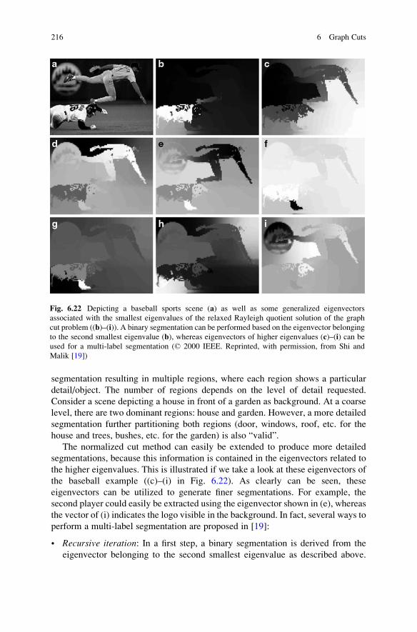
segmentation resulting in multiple regions, where each region shows a particular

detail/object. The number of regions depends on the level of detail requested.

Consider a scene depicting a house in front of a garden as background. At a coarse

level, there are two dominant regions: house and garden. However, a more detailed

segmentation further partitioning both regions (door, windows, roof, etc. for the

house and trees, bushes, etc. for the garden) is also “valid”.

The normalized cut method can easily be extended to produce more detailed

segmentations, because this information is contained in the eigenvectors related to

the higher eigenvalues. This is illustrated if we take a look at these eigenvectors of

the baseball example ((c)–(i) in Fig. 6.22). As clearly can be seen, these

eigenvectors can be utilized to generate finer segmentations. For example, the

second player could easily be extracted using the eigenvector shown in (e), whereas

the vector of (i) indicates the logo visible in the background. In fact, several ways to

perform a multi-label segmentation are proposed in [19]:

• Recursive iteration: In a first step, a binary segmentation is derived from the

eigenvector belonging to the second smallest eigenvalue as described above.

Fig. 6.22 Depicting a baseball sports scene (a) as well as some generalized eigenvectors

associated with the smallest eigenvalues of the relaxed Rayleigh quotient solution of the graph

cut problem ((b)–(i)). A binary segmentation can be performed based on the eigenvector belonging

to the second smallest eigenvalue (b), whereas eigenvectors of higher eigenvalues (c)–(i) can be

used for a multi-label segmentation (© 2000 IEEE. Reprinted, with permission, from Shi and

Malik [19])

216 6 Graph Cuts

Next, for each of the both regions, the whole method is applied again, i.e., a new

subgraph for all pixels of one region is built, spectrally solved, and so on. This

leads to a further binary partition of both regions. The recursion stops when the

normalized cut cost exceeds a certain threshold. In that case a region is not split

any further. This proceeding produces stable results but is computationally

wasteful, because only the second smallest eigenvector is used at each iteration.

The information contained in the other eigenvectors is ignored.

• Recursive splitting: Here, the generalized eigensystem is calculated only once.

After performing a binary segmentation with the second smallest eigenvector,

we can use the eigenvector of the third smallest eigenvalue to recursively

subdivide the regions by thresholding this eigenvector (e.g., by calculating a

separate threshold for each region, where the threshold is based on a subset of the

eigenvector values belonging to this region). Next, we move on to the vector of

the fourth smallest eigenvalue, which further sub-partitions the subregions, and

so on, until the normalized cut costs exceed a certain threshold (see [19] for

details). While this is computationally more efficient, some care is required here:

– There may exist eigenvectors which are not suited for partitioning, because

their values vary smoothly. A simple way of dealing with this problem is to

skip these eigenvectors, e.g., by checking the distribution of the values of the

eigenvector elements, i.e., the histogram of the element values (see [19] for

details).

– Because the segmentation is derived from a real-valued approximation, the

approximation error accumulates at each step and eventually makes the

segmentation unreliable.

• Simultaneous splitting: Here, for each pixel a vector zp is built, which

accumulates all “its” values of the eigenvectors of the M smallest eigenvalues

(i.e., for pixel p this vector contains all vm;p , where 2 � m � M). These vectors

are clustered, e.g., by a k-means algorithm intokclusters, yielding a segmentation

intok regions. Practically,k is chosen such that an over-segmentation is produced.

In a subsequent cleanup step, regions are combined again, if necessary.

Let’s now turn to some implementation issues. The first is how we should choose

the edge weights wpq . Shi and Malik proposed a weight which considers both

similarity of the appearance of pixels p and q as well as their spatial distance. As theweights should reflect the likelihood that p and q belong to the same object, wpq

should be large in case of similar appearance as well as spatial proximity. Both

terms can be combined as follows:

wpq ¼ exp� FðpÞ � FðqÞk k2

σ2F

!� exp

� XðpÞ�XðqÞk k2σ2X

�if XðpÞ � XðqÞk k < r

0 otherwise

( )

(6.18)


where FðpÞ denotes an appearance parameter, which could, e.g., be chosen to the

brightness of p, its RGB values for color images, or some more elaborate function

like a descriptor. XðpÞ denotes the position of p such that XðpÞ � XðqÞk k is the

Euclidean distance between p and q . σ2F are parameters controlling the falloff

rate of the exponential terms. If the distance between p and q exceeds a certain

maximum distance r , the wpq will become zero and therefore the threshold reffectively leads to graphs which are connected only locally.

Another point is that computing the complete generalized eigensystem

would be computationally too expensive, as D and W are matrices of size n� n,with n denoting the number of pixels. However, please note that due to local

connectivity W is usually sparse and, additionally, we’re only interested in just a

few eigenvectors. An efficient solver taking these two circumstances into account is

the so-called Lanczos method (see, e.g., [12]), which makes the running times

feasible. A usage of the Lanczos method is possible, because we can transform

the generalized eigensystem into an “ordinary” eigensystem, which is denoted by

D�1=2 D�Wð ÞD�1=2y ¼ λy.The performance of the method is illustrated in Fig. 6.23, where a weather image

is separated into multiple segments (multi-labeling is performed with the “recursive

splitting” method). Observe that the objects here have rather ill-defined boundaries

but could be segmented quite accurately by the system.

Fig. 6.23 Depicting a weather radar image (a) along with the multi-label segmentation (b)–(g)calculated by the normalized cut method (© 2000 IEEE. Reprinted, with permission, from Shi and

Malik [19])

218 6 Graph Cuts

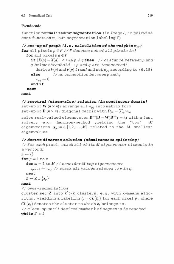
Pseudocode

function normalizedCutSegmentation (in image I, in pairwisecost function w, out segmentation labeling l�)

// set-up of graph (i.e. calculation of the weights wpq)for all pixels p 2 P // P denotes set of all pixels in I

for all pixels q 2 Pif XðpÞ � XðqÞk k < r && p 6¼ q then // distance between p andq below threshold ! p and q are “connected”

derive FðpÞ and FðpÞ from I and set wpq according to (6.18)else // no connection between p and q

wpq 0

end ifnext

next

// spectral (eigenvalue) solution (in continuous domain)set-up of W (n� n): arrange all wpq into matrix form

set-up of D (n� n): diagonal matrix with Dpp ¼P

q wpq

solve real-valued eigensystem D�12 D�Wð ÞD�1

2y ¼ λy with a fastsolver, e.g. Lanczos-method yielding the “top” Meigenvectors ym;m 2 1; 2; . . . ;M½ � related to the M smallest

eigenvalues

// derive discrete solution (simultaneous splitting)// for each pixel, stack all of itsM eigenvector elements ina vector zpZ fgfor p ¼ 1 to n

for m ¼ 2 to M // consider M top eigenvectorszp;m�1 vm;p // stack all values related to p in zp

next

Z Z [ zp�

next// over-segmentation

cluster set Z into k0 > k clusters, e.g. with k-means algo-

rithm, yielding a labeling lp ¼ CL zp� �

for each pixel p, where

CL zp� �

denotes the cluster to which zp belongs to.

// clean-up until desired number k of segments is reached

while k0 > k


merge two segments into one, e.g. according to k-way mini-mum cut criterion (see [19] for details) (i.e. adjustlabeling l)k0 k0 � 1

end while// set solution to current labelingl� l

References

1. Boykov J, Funka-Lea G (2006) Graph cuts and efficient N-D image segmentation. Int J

Comput Vis 70(2):109–131

2. Boykov J, Jolly MP (2001) Interactive graph cuts for optimal boundary and region segmenta-

tion of objects in N-D images. Int Conf Comput Vis 1:105–112

3. Boykov J, Kolmogorov V (2004) An experimental comparison of min-cut/max-flow

algorithms for energy minimization in vision. IEEE Trans Pattern Anal Mach Intell 26

(9):1124–1137

4. Boykov J, Veksler O, Zabih R (2001) Fast approximate energy minimization via graph cuts.


5. Carreira J, Sminchisescu C (2010) Constrained parametric min-cuts for automatic object

segmentation. Proc IEEE Int Conf Comput Vis Pattern Recognit 23:3241–3248

6. Carreira J, Sminchisescu C (2012) CPMC: automatic object segmentation using constrained

parametric min-cuts. IEEE Trans Pattern Anal Mach Intell 34(7):1312–1328

7. Cook WJ, Cunningham WH, Pulleyblank WR, Schrijver A (1998) Combinatorial optimiza-

tion. Wiley, New York. ISBN 978–0471558941

8. Dinic EA (1970) Algorithm for solution of a problem of maximum flow in networks with

power estimation. Soviet Math Doklad 11:1277–1280

9. Ford L, Fulkerson D (1962) Flows in networks. Princeton University Press, Princeton. ISBN

978–0691146676

10. Geman S, Geman D (1984) Stochastic relaxation, Gibbs distributions, and the Bayesian

restoration if images. IEEE Trans Pattern Anal Mach Intell 6(6):721–741

11. Goldberg A, Tarjan R (1988) A new approach to the maximum flow problem. J Assoc Comput

Mach 35(4):921–940



13. Grieg B, Porteous B, Scheult A (1989) Exact maximum a posteriori estimation for binary

images. J R Stat Soc B 51(2):271–279

14. Kolmogorov V, Zabih R (2004) What energy functions can be minimized via graph cuts? IEEE

Trans Pattern Anal Mach Intell 26(2):147–159

15. Mishra AK, Aloimonos Y, Cheong L-F, Kassim AA (2012) Active visual segmentation. IEEE

Trans Pattern Anal Mach Intell 34(4):639–653

16. Rother C, Kolmogorov V, Blake A (2004) GrabCut – interactive foreground extraction using

iterated graph cuts. ACM Trans Graphic 23(3):309–314

17. Roy S (1999) Stereo without epipolar lines: a maximum-flow formulation. Int J Comput Vis 34

(2/3):147–161

18. Roy S, Cox IJ (1998) A maximum-flow formulation of the n-camera stereo correspondence

problem. Int Conf Comput Vis 6:492–499

19. Shi J, Malik J (2000) Normalized cuts and image segmentation. IEEE Trans Pattern Anal Mach

Intell 22(8):888–905

220 6 Graph Cuts

Chapter 7

Dynamic Programming (DP)

Abstract Some problems of computer vision can be formulated in a recursive

manner. For this class of problems, the paradigm of dynamic programming (DP)

represents an interesting tool in order to obtain a fast discrete solution. Here, the

overall problem is broken down into a series of sub-problems, which are built upon

each other and can therefore be solved iteratively. This way computation can be

sped up considerably through the reusage of information gathered in already solved

sub-problems. This chapter starts with presenting the well-known method of

Dijkstra as an example of shortest path algorithms, which are closely related to

DP. “Intelligent scissors” interactively segmenting an image are one example

application. Furthermore, this chapter deals with two ways of applying the dynamic

programming paradigm. First, dynamic programming is applicable if optimal

positions or labels are to be found for a sequence of points, where the optimality

criterion for each point depends on its predecessor(s). The task of calculating active

contours can be reformulated in this manner. Second, some problems show a

treelike structure, which makes a recursive formulation possible, too. The recogni-

tion of objects which are modeled as a configuration of parts is one example of this.

Dynamic programming (often abbreviated by DP) is based on the work of Bellman

and is more a paradigm than a specific algorithm. It can accelerate discrete optimiza-

tion considerably if the problem at hand has a special structure. Dynamic program-

ming algorithms try to split the overall problem into a series of smaller sub-problems,

which are easier to solve. Typically, the solution of the first sub-problem is more or

less obvious or at least very simple. The other sub-problems get increasingly complex

but can be solved quite fast as well in a recursive manner, because their solution is

based on the solutions of the sub-problems they depend on.

In other words, we start by solving the smallest sub-problem and then iteratively

go on with solving increasingly larger sub-problems, where we can make use of the

solutions already obtained. This is a typical bottom-up approach, where information

about the solutions of the sub-problems is stored and can then be reused when

calculating the solutions of the larger problems.



221

However, such a proceeding requires that there exists a direct relation between

the larger sub-problems and the sub-problems they depend on. This relation is

termed the Bellman equation in literature.

In order to decide whether the dynamic programming paradigm is applicable for

a given problem, we can check whether the problem features the following two key

characteristics:

• Optimal substructure: This means that the solution of the problem can be

derived from a combination of the solutions of some sub-problems. Usually,

this is the case if a recursive problem formulation is possible.

• Overlapping sub-problems: Ideally, the solution of all sub-problems can be

calculated by the same proceeding, e.g., by applying the same recursive formula.

This is desirable because it allows for a straightforward implementation. Hence,

this property states that there are at most just a few calculation rules for the

solution of the sub-problems. If every sub-problem had its own rules, an efficient

implementation in a computer program would not be possible.

After this short rather general introduction, we directly go on to some application

fields of dynamic programming, because a deeper understanding of the working

principle behind dynamic programming is probably best obtained by examining the

applications. We start with shortest path algorithms and subsequently present

dynamic programming along a sequence and in a tree.

7.1 Shortest Paths

7.1.1 Dijkstra’s Algorithm

Consider a graph G ¼ N;Eð Þ consisting of nodes of the set N, which are linked by

edges of the setE, where each edge eij has a nonnegative weightwij. A quite common

question is to find a shortest path between two nodes u and v, i.e., the path from u to vwhich has the smallest sum of edge weights. One well-known application of this

shortest path algorithm is the problem to find the shortest route in a satnav system.

Here, the eij corresponds to roads and the wij to their lengths.

Such problems can be solved with Dijkstra’s algorithm (see [3]). Dijkstra makes

use of the fact that if a specific path between u and v actually is the shortest path

between these two nodes, the sub-path between u and any “intermediate” node ralong the path as well as the sub-path between r and v are shortest paths, too.

This observation directly leads to a recursive formulation of the problem, where

the total length of the shortest path between u and v can be calculated based on the

lengths of the shortest paths between u and all neighbors of v. Let luv be the length ofthe shortest path between u and v. Furthermore, RðvÞ shall denote the set of all

neighbors of v, where each ri 2 RðvÞ is connected to v by just one edge with weight

222 7 Dynamic Programming (DP)

wriv. We can then calculate luv by examining the luri as well as the wriv. The relation

between luv and the luri is given by

luv ¼ minri2RðvÞ

luri þ wrivð Þ (7.1)

The relation of (7.1) helps to identify the shortest path as follows. Suppose we

pick one node xwhere the shortest path length lux between u and x is already known.This information can now be utilized for an update of the of the shortest path length

estimates between u and all neighbors of x: suppose that for a neighbor ri of x; there

already exists an estimate lkuri of the length of the shortest path form u to ri. From

(7.1) we now know that the new estimate under consideration of x can be set to

lkþ1uri¼ min lkuri ; lux þ wxri

� �.

We can start at u and then iteratively expand the knowledge of the shortest pathsacross the graph by applying the same update formula at each iteration. This clearly

shows that the problem has optimal substructure, which relates Dijkstra’s method

closely to dynamic programming.

Please observe that such a proceeding does not try to go straight to the destina-

tion node. Instead, the algorithm assumes that the destination will be reached

anyway sooner or later and just goes on until exactly this happens. In other

words, because the scheme performs an iterative update of the path lengths of allneighbors, it has no bias that the nodes under consideration gravitate quickly toward

the destination node.

Before we describe how algorithm works in detail, let’s first state that the node

set N can be split into three disjoint subsets in the following way:

• Analyzed nodes: This setAcontains all nodes where the calculation is “finished”,i.e., the lengths of the shortest path from u to r; r 2 A are already known.

• Candidate nodes: Nodes of this setB already have been considered at least once.

When we use the algorithm presented below, this means that there is at least one

estimate for the length of the shortest path betweenu and xk; xk 2 B. In contrast tothe nodes of set A, however, not all edges which connect xk to some other node

have been examined yet. Therefore, it might still be possible to reduce the

shortest path length estimate. At each iteration, Dijkstra’s algorithm picks one

node out of set B.• Unvisited nodes: This set C consists of nodes which have not been considered

at all, i.e., have never been visited so far. Therefore, currently there is no

estimate for the length of the shortest path from u to any node of this set

available yet.

Utilizing this node classification, we can assign a cost lur between the starting

node u and more and more nodes r and try to expand the set of known shortest pathsto the neighbors of r as the iteration proceeds. Because usually we don’t want to justcalculate the lowest cost but also the route of the shortest path, the algorithm

additionally remembers the incoming edge which belongs to the shortest path

7.1 Shortest Paths 223

from u to r for each node of setA. With the help of this information, the shortest path

can be traced back from any node of set A to the starting node u.The proceeding of the scheme first initializes the node sets withA ¼ fg (empty),

B ¼ uf g (contains just the starting nodeu), andC ¼ N � uf g. The length of the startnode u to itself is equal to zero: luu ¼ 0. All other lengths are set to infinity as we

don’t know anything about these values yet. The iteration which reveals the shortest

paths comprises the following steps, which are performed repeatedly (see also

flowchart in Fig. 7.1):

1. Take the node xk from B, which has the lowest current shortest path estimate:

xk ¼ argmin luxkð Þ . This node is considered most promising when trying to

enlarge the set A.2. Examine all neighbors ri of xk which are not part of A already (ri =2 A). If luxkþwxkri < luri, then we have found a shorter path from u to ri. This new estimate of

the shortest path from u to ri passes through xk. We can update the shortest path

length estimate according to luri ¼ luxk þ wxkri . In order to be able to restore the

route of the shortest path, we additionally remember a pointer to xk for each

updated ri, i.e., the edge s rið Þ between ri and xk. We also transfer ri toB, if it still ispart of C (i.e., visited for the first time).

3. Transfer xk from B to A , because now all edges connecting xk are already

examined and consequently luxk will not change any longer.

This iteration terminates if either the destination node v is added to A (and hence

the desired solution is found, so we can stop the iteration) or the setB gets empty. If

B gets empty before v is reached, this means that v is unreachable from u. If v is

reached, we know the total sum of edge weights along the shortest path. In order to

recover the course of the shortest path, we trace back the stored edges, starting with

sðvÞ, and collect them in the set S, until we reach the start node u.Efficient implementations of the method have a complexity in the order of

O E � logðNÞð Þ.

S

E

InitSelect node xkwith shortestpath length

Destinationnode u ∈A ?

yes

no

Update pathlength estimates

of neighbors of xk

Update nodesets A, B,and C

Fig. 7.1 Flowchart of the Dijkstra algorithm


Example

The working principle of the method is best shown with a small toy example.

Consider the graph shown in Fig. 7.2, where the shortest path from node a to nodeg has to be found. The weights of the edges along the path are given next to

each edge.

In the initialization stage of Dijkstra’s algorithm, the node sets are initialized as

follows:A ¼ fg,B ¼ af g, andC ¼ b; c; d; e; f ; gf g. The distance estimate to a is setto zero (laa ¼ 0), whereas all other distance estimates are set to infinity (lab ¼ lac¼ . . . ¼ lag ¼ 1). A complete overview of the proceeding of the method for this

example can be seen in Table 7.1.

In the first iteration, we pick node a from B (as it is the only node of this set) and

update the distance estimates of the neighbors b, c; and e according to the weights ofthe edges between these nodes and node a. Moreover, these nodes are transferred

from setC toB. Because all of its edges are now examined, a is transferred fromB to

A (for a summary, see column “Iter. 1” of Table 7.1). In order to be able to trace

back the shortest path, set sðbÞ ¼ sðcÞ ¼ sðeÞ ¼ a.Iteration 2 starts with picking the node of set B with the smallest distance

estimate, which is node b. The only neighbor of bwhich is not examined completely

yet is node d , which is transferred to B. The distance estimate is set to lad ¼ labþwbd ¼ 2þ 6 ¼ 8, sðdÞ ¼ b. All other updates can be seen in column “Iter. 2” of

Table 7.1.

The third iteration (see “Iter. 3”) begins with the selection of node e, which can

be used for a first estimate of laf and lag. Moreover, we can see that the route tod viae

is shorter than the previous estimate, as lae þ wed ¼ 4þ 2 ¼ 6 < 8. Consequently,

we reduce lad to six and change sðdÞ to e. From now on, each node is visited at least

once, and accordingly set C gets empty.

The main impact of iterations 4 and 5 is the reduction of laf from 12 to 10 and

7, respectively, because we find a shorter path for f in each step. Additionally, sðf Þ isfinally changed to d.

In the last iteration, we find a better route to the destination node g. Tracing backthe predecessors, the path g! f ! d ! e! a is revealed (see Fig. 7.3).

a

c f

g

edb

5 5

18

4

8

4

2

2

6

Fig. 7.2 Exemplifying a

graph, where the shortest

path from node a to node ghas to be found. The edge

weights are given next to

each edge


Tab

le.7.1

SummarizingtheproceedingofDijkstra’s

algorithm

fortheexam

ple

shownin

Fig.7.2.

Init

Iter.1

Iter.2

Iter.3

Iter.4

Iter.5

Iter.6

Afg

a fg

a;b

fg

a;b;e

fg

a;b;c;e

fg

a;b;c;d;e

fg

a;b;c;d;e;f

fg

Bafg

b;c;e

fg

c;e;d

fg

c;d;f;g

fg

d;f;g

fg

f;g

fg

gfg

Cb;c;d;e;f;g

fg

d;f;g

fg

f;g

fg

fgfg

fgfg

minðBÞ

ab

ec

df

l aa

00

00

00

0

l ab

12

22

22

2

l ac

15

55

55

5

l ad

11

86

66

6

l ae

14

44

44

4

l af

11

112

107

7

l ag

11

112

12

12

11

sðbÞ

–a

aa

aa

a

sðcÞ

–a

aa

aa

a

sðdÞ

––

be

ee

e

sðeÞ

–a

aa

aa

a

sðfÞ

––

–e

cd

d

sðgÞ

––

–e

ee

f


Pseudocode

function shortestPathDijkstra (in graph G ¼ N;Eð Þ, in start

node u, in destination node v, in edge weighs W ¼ wij

� �, out

edges of shortest path S ¼ sðxÞf g// initializationA fgB uf g; luu 0C N � uf g// main looprepeat

// step 1: select the most “promising” node xk of Bluxk FLOAT_MAXfor all nodes b of B

if lub < luxk thenluxk lubxk b

end ifnext// step 2: examine all neighbors ri of xk which are =2Afor all nodes ri linked to xk by an edge exkri && ri=2A

if luxk þ wxkri < luri then// shorter path between u and ri foundluri luxk þ wxkri // update shortest path estimates rið Þ exkri // remember edge for path tracingif ri 2 C then

B B [ rif gC C� rif g

end ifend if

next// step 3: update node setsA A [ xkf gB B� xkf g

until xk ¼¼ v (convergence) || B ¼¼ fg (abort)// trace back shortest path

a

c f

g

edb

55

18

4

8

4

2

2

6

Fig. 7.3 Same path as in

Fig. 7.2, where the shortest

path from node a to node g isshown in bold green


xk vrepeat

S S [ s xkð Þf gset xk to the “other” node of s xkð Þ

until xk ¼¼ u (start node reached)

A disadvantage of Dijkstra’s algorithm is that it does not make any effort to

directly search the shortest path from u to the destination node v. This just happens“accidentally” sooner or later. As a consequence, the scheme does a lot of unneces-

sary work in unfavorable situations.

In order to overcome this weakness, some variants have been proposed over the

years. Especially to mention is the A* method [10], which is a variant of Dijkstra’s

algorithm, which tries to select a “better” node xk at each iteration than the original

algorithm does. In this context, “better” means that the node choice is steered

toward the destination node.

To this end, the node selection in step 1 is modified such that the decision value

not only reflects the cost of the path traveled so far but also includes a term dxkv ,which estimates the distance to the destination node. We can now define the

modified decision value lduxk by lduxk ¼ luxk þ dxkv. Consequently, the A* algorithmselects the node xk of B with the lowest lduxk .

However, some care is required, because the dxkv must not overemphasize the

distance to the destination node. Otherwise we might choose nodes with a current

shortest path estimatewhich could be reduced ifwe had considered all of its neighbors.

This situation can be avoided if the following relation holds: dxv � dyv�� wxy ,

i.e., the absolute difference of the d�v ’s between adjacent nodes x and y is at most

the weight wxy of the edge connecting these two nodes.

7.1.2 Example: Intelligent Scissors

Shortest path algorithms can also be used for vision applications. One method

utilizing shortest paths is termed “intelligent scissors” [11], which is a scheme for

an interactive segmentation of images.

The segmentation of images, i.e., the separation of one or more objects shown in

an image from the background, is a difficult task, among other reasons because both

objects as well as the background can be highly structured, which makes it difficult

to recognize them as connected regions. As a consequence, a fully automatic

segmentation is often error-prone. Therefore, an interactive scheme for segmenta-

tion, which is guided by user input, is suggested in [11].

The general proceeding of the method is an interactive derivation of a curve,

which separates an object from its surrounding background. To this end the user

first selects a “seed point” where the curve should start. This point is placed at the

boundary of the object to be segmented. Subsequently, the system automatically

calculates “optimal” segmentation curves from the seed point to every other pixel ofthe image. These curves should follow the object boundary as much as possible. As


the user moves a mouse pointer within the image, the system displays the “optimal”

curve from the seed point to the pixel currently covered by the mouse pointer. If the

user wants to accept the curve as part of the object boundary, she/he can select it via

mouse click.

In the next step, the user can select another starting point in order to define the

next segment, probably near the end of the just determined curve segment. Again,

the system calculates optimal curves to all other points, and one of them is selected

by the user. This process is repeated until the segmentation is fully defined.

Now let’s turn to the question how to calculate “optimal” curves from a seed point

to all other pixels. To this end, the image is represented by a graph, where each pixel

is represented by a node. Neighboring pixels p and q are connected by edges epq suchthat each pixel is connected to all pixels in its 8-neighborhood (see Fig. 7.4).

Consequently, a segmentation can be represented by a set of contiguous edges (see

edges marked green in the right part of Fig. 7.4). In order to select the edges which

represent a segmentation, a weight w p; qð Þ is attributed to each edge epq. The weightshould reflect the suitability of an edge of being part of the segmentation. High

probabilities of being part of an object boundary should lead to low edge weights.

Within this setup, we can determine the “optimal” segmentation curve from start

pixel s to a termination pixel twith a shortest path algorithm. In order to calculate the

shortest paths between s and all other pixels of the image, Mortensen et al. [11]

utilize a variant of Dijkstra’s algorithm, which proceeds until all pixels of the image

are contained in set A.The edge weightsw p; qð Þbetween the pixelsp andq are composed of three terms:

• Laplacian: Second-order derivative information can be useful in order to judge

whether a pixel p is likely to be located on the boundary of an object. Usually,

the object intensity or color is different from the background. Positions where

the second derivative of image intensity changes its sign (zero-crossing) indicate

object boundaries, because zero-crossings in the second derivative correspond to

local maxima (or minima) of the gradient. In order to approximate the second

Fig. 7.4 Exemplifying the representation of a pixel grid as a graph. Each pixel (square) is

represented by a node (circle), which is connected to its eight neighbors (left grid: one pixel is

highlighted red as an example). Right grid: a segmentation is represented by contiguous edges in

bold green


derivative of the image intensities, the image I can be convolved with a

Laplacian kernel KL , i.e., LðxÞ ¼ IðxÞ � KL , where * denotes the convolution

operator. The Laplacian-based edge weight wLðqÞ can be calculated as follows:

ð7:2Þwhere denotes the 8-neighborhood of pixel q. In other words,wLðqÞ, whichhas the meaning of a cost, is set to zero if a zero-crossing of L occurs between

pixel q and any of its 8 neighbors; otherwise it is set to one.

• Gradient Magnitude: It is well known that gradient strength is a good indicator

for object boundaries, too. Usually, the larger the gradient magnitude GðqÞ ¼ffiffiffiffiffiffiffiffiffiffiffiffiffiffiffiffiffiffiffiffiffiffiffiffiffiffiffiffiffiffiffiffiffiffiffiffiffiffiffiffiffiffiffiffiffiffiffiffiffiffiffiffiffi@IðqÞ @x=ð Þ2 þ @IðqÞ @y=ð Þ2

qof a pixel q gets, the higher is the probability of q

being part of an object boundary. Consequently, we can use GðqÞ as anothercontribution wGðqÞ to w p; qð Þ:

wGðqÞ ¼ 1� GðqÞGmax

(7.3)

where Gmax is the maximum gradient of the entire image, which ensures that

wGðqÞ is between 0 and 1. Please note that wGðqÞ is small if GðqÞ is near themaximum gradient and large otherwise.

• Gradient direction: Object boundaries typically don’t have many sharp changes

of direction when we move from one boundary pixel to a second one being

adjacent to it. Therefore, the third term wD p; qð Þ should reflect this bias to

smooth edges by penalizing sharp changes in boundary direction. To this end,

gradient directions can be used as follows. Consider the direction dðpÞ ¼@IðpÞ @y= ;�@IðpÞ @x=½ �T, which is perpendicular to the direction of the intensity

gradient of p and usually reflects the direction of the object boundary if the

boundary is straight. We can therefore compare dðpÞ as well as dðqÞ with the

direction l p; qð Þ of the link between p and q. If l p; qð Þ deviates much from dðpÞ ordðqÞ, this indicates that we have a sharp change of boundary direction. “Smooth”

boundaries in turn have only small deviations between l p; qð Þ and dðpÞ or dðqÞ.Consequently, wD p; qð Þ should be small for smooth boundaries. The dot product

�h i is a good measure for direction differences, and the authors of [11] suggest to

calculate wD p; qð Þ by

wD p; qð Þ ¼ 1

π

1

cos dðpÞ; l p; qð Þh ið Þ þ1

cos l p; qð Þ; dðqÞh ið Þ�

with l p; qð Þ ¼ q� p if dðpÞ; q� ph i � 0

p� q if dðpÞ; q� ph i < 0

(7.4)

Overall, w p; qð Þ is calculated by


w p; qð Þ ¼ α � wLðqÞ þ β � wGðqÞ þ γ � wD p; qð Þ (7.5)

where α, β; and γ are weighting terms reflecting the relative influence of the

corresponding term and are chosen empirically.

The application of (7.5) in a shortest path algorithm together with interactive

user assistance yields a quite powerful and easy to handle method. Figure 7.5

illustrates the proceeding as well as the result. There you can see how the user

moves the mouse pointer after selecting a seed point (white curve). Different

positions on the white curve involve different shortest paths, which follow the

true object contour as much as possible, and the branch to the current mouse pointer

position (orange – true boundary, green paths: “branches” through the background

to some selected mouse pointer positions). The orange path is the shortest path to

the last known mouse pointer position as calculated by the system. As can easily be

seen, this path is a very good approximation of the true object contour.

The image in Fig. 7.6 illustrates that the method works well even in challenging

situations. This exemplifies the performance of the method, which is achieved with

very little user input.

Usually, the user-selected endpoint does not lie exactly on the object boundary.

A convenient possibility to “correct” this is to select the next starting point some

pixels away from the current endpoint such that it coincides with the object

boundary. Another possibility is to use the snap-in functionality of the algorithm,

which forces the mouse pointer to positions of maximum gradient magnitude within

a small neighborhood, e.g., 11�11 pixel.

Fig. 7.5 Exemplifying the proceeding of the intelligence scissors method (Mortensen and Barett

[11] © 1995 Association for Computing Machinery, Inc. Reprinted by permission)


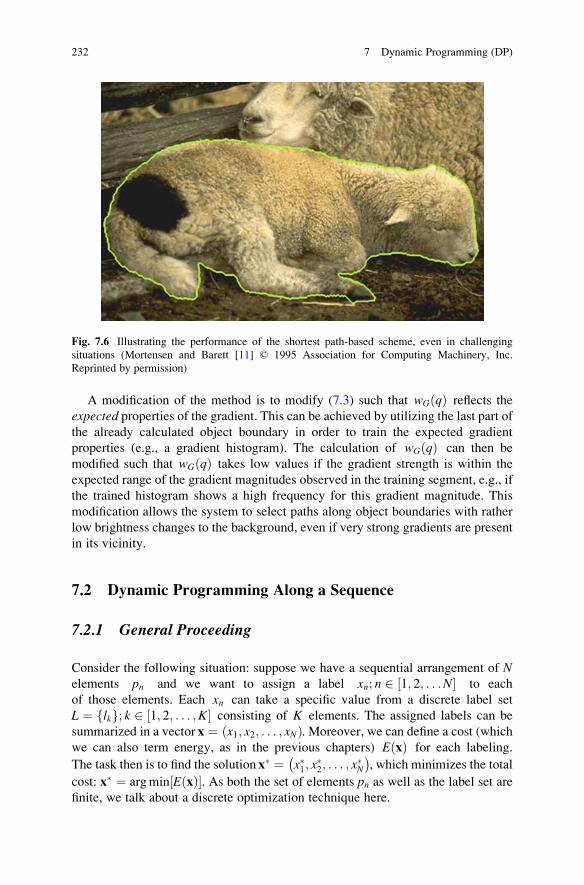
A modification of the method is to modify (7.3) such that wGðqÞ reflects the

expected properties of the gradient. This can be achieved by utilizing the last part ofthe already calculated object boundary in order to train the expected gradient

properties (e.g., a gradient histogram). The calculation of wGðqÞ can then be

modified such that wGðqÞ takes low values if the gradient strength is within the

expected range of the gradient magnitudes observed in the training segment, e.g., if

the trained histogram shows a high frequency for this gradient magnitude. This

modification allows the system to select paths along object boundaries with rather

low brightness changes to the background, even if very strong gradients are present

in its vicinity.

7.2 Dynamic Programming Along a Sequence


Consider the following situation: suppose we have a sequential arrangement of Nelements pn and we want to assign a label xn; n 2 1; 2; . . .N½ � to each

of those elements. Each xn can take a specific value from a discrete label set

L ¼ lkf g; k 2 1; 2; . . . ;K½ � consisting of K elements. The assigned labels can be

summarized in a vector x ¼ x1; x2; . . . ; xNð Þ. Moreover, we can define a cost (which

we can also term energy, as in the previous chapters) E xð Þ for each labeling.

The task then is to find the solution x� ¼ x�1; x�2; . . . ; x

�N

� �, which minimizes the total

cost: x� ¼ argmin E xð Þ½ �. As both the set of elements pn as well as the label set arefinite, we talk about a discrete optimization technique here.

Fig. 7.6 Illustrating the performance of the shortest path-based scheme, even in challenging

situations (Mortensen and Barett [11] © 1995 Association for Computing Machinery, Inc.

Reprinted by permission)


In many applications, E xð Þ can be defined to have the following structure (see

also [6]; examples will follow later on):

E xð Þ ¼XN

n¼1Dn xnð Þ þ

XN�1

n¼1V xn; xnþ1ð Þ (7.6)

Usually, theDn xnð Þ are data-dependent terms, which describe the cost of assigning

the label xn to the nth element of the sequence, based on some observed data. The

V xn; xnþ1ð Þ represent priors, which should reflect the probabilities of a joint labelingof two successive elements of the sequence. They are independent of the data and can

therefore be calculated in advance for any possible combination of labels.

A closer look at (7.6) reveals that the energy defined here has the same structure

as many energies utilized in the previous chapters: it is also composed of two terms,

where one reflects the fidelity to some observed data, whereas the other incorporates

some kind of prior knowledge, e.g., smoothness constraints. However, observe that

the sums are taken along a (one-dimensional) sequence of elements, which is

opposed to the two-dimensional sums along a pixel grid we already encountered.

In order to find the solution x�, dynamic programming can be used. The special

case that the elements pn are arranged along a one-dimensional sequence enables us

to formulate the calculation of the energy in a recursive manner. Consider a labeling

of a part of the sequence x1; x2; . . . ; xnð Þ; n � N. The cost for this labeling depends

on the cost of the labeling of the subsequence x1; x2; . . . ; xn�1ð Þ where the last

element pn is excluded as follows:

E x1; x2; . . . ; xnð Þ ¼ E x1; x2; . . . ; xn�1ð Þ þ Dn xnð Þ þ V xn�1; xnð Þ (7.7)

Clearly, this is a recursive formulation. This fact can be exploited in dynamic

programming by first calculating the minimum energy for a part of the sequence

(i.e., solving a smaller sub-problem) and then reusing this information when

extending the sequence by one additional element (i.e., extending the solution to

a larger problem), until the minimum cost for the entire sequence is found.

In practice, for each element pn of the sequence, a table Bn can be calculated,

where each entry of Bn xnð Þ denotes the minimum cost of the subsequence from the

first to the nth element pn , under the assumption that the label xn takes a specific

value lk. Therefore, eachBn is composed ofK elements. The initialization for the first

element of the sequence is trivial, because we can simply set B1 x1ð Þ ¼ D1 x1ð Þ. Theentries of all other tables can be calculated via the recursive formulation:

Bn xnð Þ ¼ Dn xnð Þ þminxn�1

Bn�1 xn�1ð Þ þ V xn�1; xnð Þð Þ (7.8)

In other words, after starting with the trivial calculation of the minimum costs for

the first table B1, we can recursively extend the solution by one element in each step

according to (7.8). Observe that previously computed tablesBn�1 are reused in a lateriteration, which is a typical characteristic of the dynamic programming paradigm.

7.2 Dynamic Programming Along a Sequence 233

This speeds up calculations, because the reusage of previous computations

accelerates the solution of each sub-problem significantly.

Up to now, we just calculate minimum costs, but we haven’t determined the

optimal labeling yet. However, as soon as the last element is reached, we can

determine the labeling of the last element by examining the values of BN xNð Þ: Thesolution x�N can be identified such that the energy associated to x

�N becomes minimal:

x�N ¼ argminxN

BN xNð Þð Þ . Once x�N is determined, we can trace back the solution

according to

x�n ¼ argminxn

Bn xnð Þ þ V xn; x�nþ1

� �� (7.9)

until the first element of the sequence is reached. Again, we can see that previously

computed Bn xnð Þ are reused to find the solution.

To sum it up, the general proceeding consists of two steps (Fig. 7.7):

1. Forward step: First, the optimal costs Bn xnð Þ under the assumption that the last

element of the sequence is labeled with the specific value are calculated recur-

sively using (7.8) and stored in the tables Bn while moving “forward” from the

first element to the last.

2. Backward step: Once the optimal costs are known, we can trace back the

solution according to (7.9) while moving “backward” from the end of the

sequence to the beginning.

The complexity of the algorithm is given by O NK2ð Þ , because we have Ntables to be filled, where each of them consists of K entries. The time necessary

for calculating each table entry is of OðKÞ. Without giving any details here, let’s

note that this complexity can be reduced in many cases through the usage of

so-called distance transforms (e.g., the interested reader is referred to [4]).

Observe that the problem given here can also be represented by a graph

(see Fig. 7.8). Each element of the (horizontally arranged) sequence is represented

S

E

n=1Calculatevalues oftable Bn

Last elem(n>N)?

yes

no

Incre-ment n

n=NCalculate

opt. label x*n

Deccre-ment n

First elem(n<1)?

yes

no

Fig. 7.7 Flowchart of the general dynamic programming algorithm flow. The forward step can be

seen in the top row, the backward step in the bottom row


by K nodes (one vertical column in Fig. 7.8), which amounts to NK nodes for

the whole sequence. Each node is connected to all K nodes of the subsequent

element, which results in NK K � 1ð Þ edges in total. Moreover, a weight

Dnþ1 xnþ1 ¼ lk2ð Þ þ V xn ¼ lk1; xnþ1 ¼ lk2ð Þ can be attributed to the edge from

node n; k1ð Þ to node nþ 1; k2ð Þ . Additionally, two “special” nodes s and t areintroduced (red nodes), where the edges from s to 1; kð Þ are weighted byD1 x1 ¼ lkð Þ,whereas all edges to node t have weight zero. Figure 7.8 shows such a situation withN ¼ 6 and K ¼ 4.

With this setup, it is possible to obtain the solution by an algorithm, which finds

the shortest path from s to t . If we apply Dijkstra’s algorithm, for example, the

overall complexity is of O NK2 � log NKð Þð Þ (because there are approximately NK2

edges and NK nodes). Compared to the recursive dynamic programming approach,

the higher complexity of Dijkstra’s algorithm can be explained by the fact that those

algorithms can handle more general situations, i.e., graphs with cycles. The DP

method presented here is faster, because it exploits the special structure of the

problem. This is another piece of evidence that, in general, optimization methods

specializing in the problem at hand also are very fast.

7.2.2 Application: Active Contour Models

Now that the theory is clear, let’s turn to the question which problems can be

formulated such that their solution can be obtained by finding the optimal path

through a sequence of points. Interestingly, it turns out that the method outlined

above can be applied to the problem of finding a suitable deformable curve, which

we encountered when dealing with active contours (see also Chap. 4).

Briefly summarized, active contours try to find a curve which fits best to the

observed data, i.e., is located upon locations of high intensity gradient, but also

satisfies some smoothness constraints, i.e., its first- and second-order derivatives

should be rather low. The “classical” approach to find a solution is to set up an

energy functional, which is based on data fidelity (“external energy”) as well as

smoothness constraints (“internal energy”), and obtain a solution by a variational

approach, which seeks a solution of the Euler-Lagrange equation derived from the

functional.

However, a problem with this proceeding is that a solution satisfying the Euler-

Lagrange equation only provides a necessary condition for optimality. Consequently,

s t

Fig. 7.8 Illustrating how the problem of finding a sequence of minimum cost can be represented

by a graph (see text for details)


http://dx.doi.org/10.1007/978-1-4471-5283-5_4

there is no guarantee that the result is a global or even at least a local minimum in fact.

Moreover, the calculations involve the estimation of higher-order derivatives, which

are typically numerically derived from discrete data and therefore prone to sensor

noise. In contrast to that, the DP approach guarantees to find the global optimum

within the specified search space. However, it is a discrete optimization technique, so

if we want to apply it to find a continuous contour, we must find a way to reformulate

it as a discrete optimization problem (see, e.g., [1]).

Discretization can be done if we approximate the contour to be estimated by a

finite set of N control points pn; 1 � n � N . Furthermore, the location xn of each

control point can be approximated by a finite set of K discrete positions (see [6]).

This approximation allows us to use the model described in the previous section as

follows:

• Each control point can be interpreted as a specific element of a sequence of

points.

• Each of theK possible positions of a specific control point can be interpreted as a

state (or a label) of an element of the sequence just defined.

The data-dependent term Dn xnð Þ can be derived from the intensity gradient at

position xn. Hence, theDn xnð Þ can be seen as a representation of the external energyused in variational optimization. Dn xnð Þ should be low at positions where the

gradient is high, as these positions are likely to be part of an object border. For

example, a linear dependence on the intensity gradient G xnð Þ can be used:

Dn xnð Þ ¼ 1� G xnð Þ Gmax= with

G xnð Þ ¼ffiffiffiffiffiffiffiffiffiffiffiffiffiffiffiffiffiffiffiffiffiffiffiffiffiffiffiffiffiffiffiffiffiffiffiffiffiffiffiffiffiffiffiffiffiffiffiffiffiffiffiffiffiffiffiffiffi@I xnð Þ @x=ð Þ2 þ @I xnð Þ @y=ð Þ2

q; Gmax ¼ max

x;yð Þ2IG x; yð Þ (7.10)

The pairwise cost V xn; xnþ1ð Þ can be set proportional to the distance between

successive control points, which steers the solution toward short curves. For

example, we can take

V xn; xnþ1ð Þ ¼ α � xn � xnþ1k k2 (7.11)

where �k k denotes the L2 norm and α serves as a weighting factor controlling the

relative influence of the different terms during optimization.

However, an important part of the internal energy in variational optimization is

the bending energy, which is high if the second derivative of the curve is high.

Therefore, considering the bending energy in the energy functional devalues parts

of high curvature and encourages the solution to be smooth. Second-order deriva-

tive information can be approximated by considering three successive control

points, e.g., by

H xn; xnþ1; xnþ2ð Þ ¼ β � xn � 2 � xnþ1 þ xnþ2k k2 (7.12)

Again, β is a weighting factor. H is high at positions of high curvature and

therefore penalizes such control point position combinations.


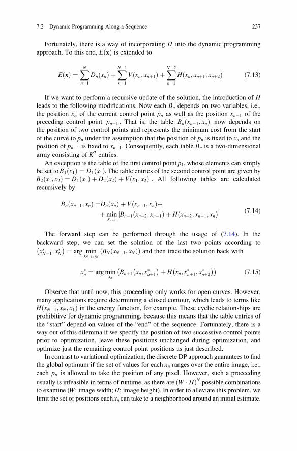
Fortunately, there is a way of incorporating H into the dynamic programming

approach. To this end, E xð Þ is extended to

E xð Þ ¼XN

n¼1Dn xnð Þ þ

XN�1

n¼1V xn; xnþ1ð Þ þ

XN�2

n¼1H xn; xnþ1; xnþ2ð Þ (7.13)

If we want to perform a recursive update of the solution, the introduction of Hleads to the following modifications. Now each Bn depends on two variables, i.e.,

the position xn of the current control point pn as well as the position xn�1 of the

preceding control point pn�1 . That is, the table Bn xn�1; xnð Þ now depends on

the position of two control points and represents the minimum cost from the start

of the curve to pn under the assumption that the position of pn is fixed to xn and the

position of pn�1 is fixed to xn�1. Consequently, each table Bn is a two-dimensional

array consisting of K2 entries.

An exception is the table of the first control point p1, whose elements can simply

be set toB1 x1ð Þ ¼ D1 x1ð Þ. The table entries of the second control point are given byB2 x1; x2ð Þ ¼ D1 x1ð Þ þ D2 x2ð Þ þ V x1; x2ð Þ . All following tables are calculated

recursively by

Bn xn�1; xnð Þ ¼Dn xnð Þ þ V xn�1; xnð Þþþmin

xn�2Bn�1 xn�2; xn�1ð Þ þ H xn�2; xn�1; xnð Þ½ � (7.14)

The forward step can be performed through the usage of (7.14). In the

backward step, we can set the solution of the last two points according to

x�N�1; x�N

� � ¼ arg minxN�1;xN

BN xN�1; xNð Þð Þ and then trace the solution back with

x�n ¼ argminxn

Bnþ1 xn; x�nþ1

� �þ H xn; x�nþ1; x

�nþ2

� �� (7.15)

Observe that until now, this proceeding only works for open curves. However,

many applications require determining a closed contour, which leads to terms like

H xN�1; xN; x1ð Þ in the energy function, for example. These cyclic relationships are

prohibitive for dynamic programming, because this means that the table entries of

the “start” depend on values of the “end” of the sequence. Fortunately, there is a

way out of this dilemma if we specify the position of two successive control points

prior to optimization, leave these positions unchanged during optimization, and

optimize just the remaining control point positions as just described.

In contrast to variational optimization, the discrete DP approach guarantees to find

the global optimum if the set of values for each xn ranges over the entire image, i.e.,

each pn is allowed to take the position of any pixel. However, such a proceeding

usually is infeasible in terms of runtime, as there are W � Hð ÞN possible combinations

to examine (W: image width;H: image height). In order to alleviate this problem, we

limit the set of positions eachxn can take to a neighborhood around an initial estimate.


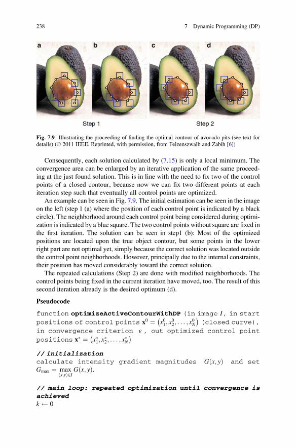
Consequently, each solution calculated by (7.15) is only a local minimum. The

convergence area can be enlarged by an iterative application of the same proceed-

ing at the just found solution. This is in line with the need to fix two of the control

points of a closed contour, because now we can fix two different points at each

iteration step such that eventually all control points are optimized.

An example can be seen in Fig. 7.9. The initial estimation can be seen in the image

on the left (step 1 (a) where the position of each control point is indicated by a black

circle). The neighborhood around each control point being considered during optimi-

zation is indicated by a blue square. The two control points without square are fixed in

the first iteration. The solution can be seen in step1 (b): Most of the optimized

positions are located upon the true object contour, but some points in the lower

right part are not optimal yet, simply because the correct solution was located outside

the control point neighborhoods. However, principally due to the internal constraints,

their position has moved considerably toward the correct solution.

The repeated calculations (Step 2) are done with modified neighborhoods. The

control points being fixed in the current iteration have moved, too. The result of this

second iteration already is the desired optimum (d).

Pseudocode

function optimizeActiveContourWithDP (in image I, in start

positions of control points x0 ¼ x01; x02; . . . ; x

0N

� �(closed curve),

in convergence criterion ε , out optimized control point

positions x� ¼ x�1; x�2; . . . ; x

�N

� �

// initializationcalculate intensity gradient magnitudes G x; yð Þ and setGmax ¼ max

x;yð Þ2IG x; yð Þ.

// main loop: repeated optimization until convergence isachievedk 0

Fig. 7.9 Illustrating the proceeding of finding the optimal contour of avocado pits (see text for

details) (© 2011 IEEE. Reprinted, with permission, from Felzenszwalb and Zabih [6])


repeat// forward step: calculate minimum costsrandomly choose two successive points xs�1 and xs as “fixedpoints” (where the position doesn’t change in currentiteration); 1 � s � N

init of recursion: Bs�1 xks�1� � ¼ Ds�1 xks�1

� �and Bs xks�1; x

ks

� � ¼Ds�1 xks�1

� �þ Ds xks� �þ V xks�1; x

ks

� �.

n sþ 1

if n > N thenn n� N // “cyclic” permutation

end ifwhile n 6¼ s

for all positions of the neighborhood around current

estimate xknfor all positions of the neighborhood around cur-

rent position estimate xkn�1calculate Bn xn�1; xnð Þ according to (7.14)

nextnextn n mod Nð Þ þ 1 // “cyclic” increment

end whilere-calculation of total cost for the two fixed points by

usage of B�s xks�1; xks

� � ¼ minxs�2

Bs�1 xs�2; xks�1� �þ H xs�2; xks�1; x

ks

� � �

// backward step: trace back and update solution

x�s xks // position is fixed

x�s�1 xks�1 // position is fixed

n s� 2

if n < 1 thenn nþ N // “cyclic” permutation

end ifrepeat

calculate x�n according to (7.15)n n� 1

if n < 1 thenn nþ N // “cyclic” permutation

end ifuntil n ¼¼ s// prepare next iteration

Δ PN

n¼1x�n � xkn

��

k k þ 1

xk x�

until Δ < ε // Δ < ε indicates convergence (Δ is cumulativedisplacement between solutions of two successiveiterations)


Please note that the pseudocode given above works for closed curves, as this is

more common than open curves. However, for closed curves we have to take care

that all indices s� 1, n� 1, etc. have to be within the bounds given by 1; . . . ;N½ �.This can be ensured by a cyclic permutation, i.e., by settingN þ 1 to 1,N to 0, and so

on. For reasons of clarity this cyclic permutation is not explicitly performed for all

indices used in the pseudocode above, but of course has to be done in a real

implementation.

7.3 Dynamic Programming Along a Tree

As we will see in this section, some applications make use of a tree-shaped model,

e.g., object recognition tasks, where the object model can be split into several parts

which are allowed to move with respect to each other. Consider so-called articulated

shapes, for example. This object model dates back to [9] and consists of several

parts, where some of them have a special relationship between each other. A model

of the human body, for example, could be split into different parts, such as head,

torso, legs, and arms. Some of the parts are “connected” to each other in a hierar-

chical manner, e.g., arms to head and hand to arm. Articulation here means that the

parts are allowed to move with respect to each other, at least up to a certain extent.

If wewant to detect objects of varying appearance due to articulation, themodeling

by a tree is an elegant way of incorporating these intra-class variations. It makes the

object detectionmethodmore invariant to those variations, because despite the overall

appearance of the object can vary considerably, the appearance of each part remains

rather static and can therefore be detected more reliably. Through usage of the

articulation model, we can bring together the individual detections of the object parts.

It turns out that dynamic programming is applicable to tree-based models as

well. The next section describes what has to be done in general such that DP can be

applied to the optimization of tree-shaped models. After that, the example of

utilizing such tree-shaped models for object recognition is presented in more detail.


Consider a tree consisting of a set of nodes N ¼ nif g; 1 � i � Nk k , where �k kdenotes the cardinality of a set (i.e., the number of its elements). Furthermore,

we can assign a label xi to each node ni with xi 2 L; Lk k ¼ K , where L ¼ lkf g;k 2 1; 2; . . . ;K½ � represents the set of labels which can be applied to each node witha cardinality of K.

Moreover, two nodes ni and nj are connected by an edge eij if they have a special

relationship. We can assign a costVij xi; xj� �

to each eij, depending on the labeling of

ni and nj.Similar to the sequence case, we can define an energy measure which considers

the labeling of the whole tree and is defined by


E x1; x2; . . . ; xNð Þ ¼ E xð Þ ¼XN

i¼1Di xið Þ þ

X

eij

Vij xi; xj� �

(7.16)

Now the task is to find a labeling x� ¼ x�1; x�2; . . . ; x

�N

� �of the whole tree which

globally minimizes (7.16).

The nature of trees prohibits the existence of cycles in the graph. This is essential

for the applicability of a DP approach, because only then it is possible to formulate

the minimization problem in a recursive manner. If the graph contains no cycles,

we can arbitrarily pick one node as the root node nr. The nodes connected to nr arecalled children of nr , and nr is called their parent node. A node can have one or

more children, but all nodes (except the root) have exactly one parent. Nodes

without children are called leaf nodes. As a tree doesn’t contain cycles, each

node ni has a certain depth di , which amounts to the number of edges between niand the root nr. The depth of ni and its parent np differ exactly by one: di ¼ dp þ 1.

An example of a tree can be seen in Fig. 7.10 (left), where the root node is marked

red and all leaf nodes are marked green.

This special structure of a tree can be exploited for a recursive formulation of the

proceeding of finding the global minimum x�. The main observation here is that the

solution of a subtree, i.e., the optimal labeling if we consider only a part of the tree,

doesn’t change if we enlarge the subtree and recalculate the solution. This is

illustrated in the right part of Fig. 7.10: suppose we already have found an optimal

labeling for the subtree marked blue. If we expand the tree by the unique parent

(marked green) and recalculate the solution of the expanded subtree, the optimal

labeling of the blue part remains unchanged.

Consequently, we can start at the leaf nodes, where the minimum cost can be

found very quickly, and then enlarge the solution by expanding the subtrees by

including parent nodes. Based on this, we can calculate the solution of the whole

tree in two steps (just as in the sequence case) as follows:

1. Forward step: In this step, we want to find the minimum costs of the subtrees

starting at the leaf nodes up to a certain node ni under the assumption that the last

element of the subtree is labeled with the specific value xi. That is, our aim is to

calculate the optimal costs Bi xið Þ for all nodes, where each Bi xið Þ is a table

consisting of K elements. One element contains the minimal subtree cost under

Fig. 7.10 Exemplifying a tree structure (left) and illustrating the suitability of trees for dynamic

programming (right)

7.3 Dynamic Programming Along a Tree 241

the assumption that xi ¼ lk, as in the sequence case. We start at the leaf nodes,

where we can simply set Bl xlð Þ ¼ Dl xlð Þ. After this, all subtrees (which after the

first step consist of only one leaf node) are expanded iteratively by inclusion of

the unique parent of the “newest” node (i.e., the node which was included most

recently in the subtree currently under consideration) until the root is reached. If

we include a node ni in the subtree, we set the Bi xið Þ according to

Bi xið Þ ¼ Di xið Þ þX

nj2Ci

min Bj xj� �þ Vij xi; xj

� �� (7.17)

where Ci denotes the set of all children of ni. Just a quick look at (7.17) reveals

that the table entries can be calculated once and be reused in later iterations when

examining the parent nodes.

Please note that in order to calculate the Bi xið Þ as defined in (7.17), the Bj xj� �

of all child nodes have to be known already. This implies certain constraints,

which have to be fulfilled when we choose the subtree which is to be expanded

next. One idea is to take only nodes where the cumulated costs of all children are

known already. An example of the proceeding is given in Fig. 7.11, where the

nodes already processed are marked blue and all possible expansions are marked

green. Observe that not all parent nodes are marked green, because the minimum

costs of the subtrees of those potential parents are not known for all subtrees. An

alternative approach is to expand the subtrees according to the depth of the

nodes. Starting with all nodes having maximum depth of the tree (which by

definition must all be leaf nodes), we can expand all nodes of the same depth at

each step. In each iteration, the depth is decreased by one until the root is

reached: decreasing by one ensures that all child nodes of the “new” nodes

have been processed already.

2. Backward step: Once the optimal costs are known, we can trace back the

solution starting at the root node and moving “backward” to the child nodes

until a leaf node is reached. At the root, we can pick the label x�r according to

x�r ¼ argminxr

Br xrð Þð Þ. If wemove backward to some childni, its labelx�i is given by

x�i ¼ argminxi

Bi xið Þ þ Vij xi; x�j

� �� (7.18)

where x�j denotes the solution of the (unique) parent nodenj of ni. This proceedingstops if the optimal labeling of all nodes is determined.

The computational complexity of this proceeding is given by O Nk k � K2ð Þ,because the runtime is largely determined by the forward step where we have to

calculate a table of optimal values for each of the nodes of the tree, each table

consists of K entries, and for each entry, OðKÞ operations are necessary for

finding the minimum according to (7.17). This can be further reduced through

the usage of distance transforms.


7.3.2 Example: Pictorial Structures for Object Recognition

7.3.2.1 Framework

A major challenge in object recognition is to handle the large intra-class variations

of some object classes. Consider the task of detecting human persons, for example.

Their appearance can vary considerably, because particularly the limbs can take

quite different positions compared to the rest of the body. Consequently, a detector

relying on a rather rigid object model will run into difficulties.

One way of tackling this problem is to split up the model into multiple parts:

Here, the model consists of a separate modeling of each part (e.g., head, torso) as

well as their spatial relationships with respect to each other. By splitting the model

into parts and allowing to move each part around its expected position (relative to

the object center), we get extra degrees of freedom allowing to handle local

deformations of the object, which could be articulation in our case. This paradigm

was first introduced in [9]. A further example is a scheme proposed by

Felzenszwalb and Huttenlocher, which is called “Pictorial Structures for Object

Fig. 7.11 Illustrating the proceeding of the forward step of the dynamic programming approach

considering a tree. At start, the costs of the leafs can be calculated (marked green in the graph on

the right side of the first row). All possible expansions are shown in the left graph of the second

row. Right to this, we can see the expansions of the next iteration. This proceeding is repeated until

the costs of the root node can be calculated (right graph of the bottom row)


Recognition” [5]. In the meantime, this quite powerful method has been refined by

the same research group (cf. [7], [8]) and shall be presented in more detail in the

following.

As already mentioned, Felzenszwalb and Huttenlocher adopt the approach of

splitting the object into different parts, too. Each part ni is described by some

appearance parameters ui and its position li. The relationship between the parts is

modeled by a graph G ¼ N;Eð Þ, where the nodes N ¼ n1; . . . ; nMf g correspond to

the M parts. A pair of nodes ni and nj is linked by an edge ni; nj� � 2 E if ni and nj

feature a characteristic relationship. The properties of this relationship, in turn, is

modeled by some connection parameters cij.Now let’s assume thatG has the form of a tree, i.e., does not contain any cycles.

For most object classes, this assumption not really constitutes a noteworthy restric-

tion. If we prohibit cycles in G, however, we are able to apply dynamic program-

ming in the object recognition process. A part-based modeling in a tree is quite

natural for many object classes. For example, in [5] it is suggested to model the

human body by a tree of ten parts, consisting of head, torso, and the four limbs,

which are split into two parts each (cf. left image of Fig. 7.12). This configuration isflexible enough for modeling considerable articulation, as the right image of

Fig. 7.12 shows.

Star-based models have also been suggested. They are composed of a root node

which covers the whole object at coarse resolution and leaf nodes where each node

covers one part of the object at a finer resolution. Hence, a star-based model is a

simple form of a tree, which consists of the root and leaf nodes only. This simple

model is suitable for modeling a large variety of object classes (like cars, different

kind of animals), where the relative position of the parts is subject to variations,

e.g., due to viewpoint change, local deformations, and so on.

During recognition, the aim of the method is to find the positions of all parts of

the searched model in a query image. This can be summarized in a vector L ¼l1; . . . ; lMð Þ called configuration by the authors of [5], where each li denotes the(center) position of a part. To this end, we can define an energy functionF, which iscomposed of two terms:

1. Appearance-based term mi li; uið Þ measuring the degree of mismatch between

model and query image if part i is placed at location li in the query image.

Usually, mi li; uið Þ is calculated by comparing the image content in a neighbor-

hood around li (appearance) with the part model (represented by the appearance

parameters ui). These appearance parameters ui have to be learned in a training

stage.

2. Deformation-based term dij li; lj; cij� �

reflecting the degree of deformation if we

place part i at location li and part j at location lj. Observe that dij li; lj; cij� �

is only

calculated if ni and nj are connected by an edge eij. During training, we can learnthe likelihood of particular location combinations. This distribution is

represented by the connection parameters cij.


In total, we have

FðLÞ ¼XM

i¼1mi li; uið Þ þ

X

ni;njð Þ2Edij li; lj; cij� �

(7.19)

Now the goal is to find the configuration L� ¼ argminL

FðLÞ which minimizes

(7.19). Observe that L� is a global minimum of L , which jointly considers the

appearance of each part as well as their relative positions. This is in contrast to (and

superior to) many other part-based methods, which first make some hard decisions

about the location of the parts and then evaluate the geometric configuration. The

problem with the joint consideration of appearance and geometry is the computa-

tional complexity, because the search space of each li is in the order of the image size,

which can amount up to millions of pixels. However, due to the structure of (7.19)

and the tree model, we can apply dynamic programming, which, together with

further speedups through distance transforms, makes a joint processing feasible.

Another advantage of this approach is that the modeling of the appearance of

each part as well as their positional arrangement takes place separately. Hence, the

object model allows for variations in the appearance of each part and deformations

of the relative positions of the parts at the same time. This kind of object represen-

tation is very generic and can be applied to a large number of object classes. Please

note that (7.19) only provides a framework, and we are free to model the parameters

mi, ui, dij, and cij such that they best fit to a particular problem at hand.

7.3.2.2 Example: Star Model with HOG Appearance

It was shown in [7] and [8] that a tree-based object model is flexible enough for a

detection of a wide variety of object classes. Felzenszwalb et al. reported similar or

leading recognition performance compared to state-of-the-art algorithms on diverse

VOC (Visual Object Classes Challenge) data sets ([12], [13]), which are


human body model of [5],

where each part is

represented by a rectangle.

Connections between parts

are indicated by red circles atthe joints between the parts.

The basic configuration can

be seen in the left part,whereas an example of an

articulated model is depicted

in the right part


acknowledged to be very challenging. The research group suggested several ways

of modeling the objects for different applications. In the following, one example of

applying this framework utilizing a so-called star model (consisting of a root node,

which is connected to multiple leaf nodes) together with appearance modeling with

the help of HOG descriptors is presented.

Modeling of Geometry

As far as the geometric modeling of the parts is concerned, the authors of [7],

[8] utilize a star model (as just mentioned), where the entire object at a coarse

resolution is used as a root. The root is connected to all parts, which are

evaluated at twice resolution compared to the root. Because of the reduction

of resolution, it is possible to model the entire object in a single more or less

rigid manner, as variations due to deformation / articulation are reduced during

downsampling, too.

The deformation between the parts and the root (second term of (7.19)) can be

measured by comparing the relative distance of part i to the position of the root (whichshall from now on be denoted by subscript one). If we take li ¼ xi; yi½ � as part positioncurrently under consideration,l1 ¼ x1; y1½ �as supposed root position, andvi as nominal

value of the relative displacement between part i and the root, we can calculate the

deformation dxi; dyi½ � by dxi; dyi½ � ¼ li � l1ð Þ � vi, i.e., the difference between actualand expected displacement between the ith part and the root. The deformation cost can

then be set to the sum of the deformations and their squares, weighted by factorswi ( �h idenotes the dot product):

di1 li; l1; vi;wið Þ ¼ wi; dih i (7.20)

where the vector di ¼ dxi; dyi; dxi2; dyi

2½ � summarizes the displacement informa-

tion. Hence, the connection parameters ci1 comprise the expected displacement vibetween the part and root as well as the weighting factors wi. The optimal splitting

of the object into parts, the relative position vi of the parts compared to the root, and

the parameters wi of the deformation cost are all learned in a training stage in an

automatic manner (see below).

Modeling of Appearance

As far as the appearance is concerned, a descriptor-based modeling is suggested in

[7], [8].1 To this end, the HOG descriptor (Histogram of Oriented Gradients) [2] is

chosen, which already has been presented in more detail in Chap. 2.

1 Please note that in [7] and especially [8] several modifications for performance-tuning are

proposed, which have been omitted here for clarity reasons. In this section, we just describe the

outline of the method. The interested reader is referred to the references for details.


http://dx.doi.org/10.1007/978-1-4471-5283-5_2

Briefly summarized, we can represent the appearance by first calculating the

intensity gradient magnitude and orientation at each pixel and quantizing the

orientation into a moderate number of discrete orientations (a typical number of

orientation bins is 9, ranging from 0 to just 180 in order to be contrast-insensitive).Furthermore, the image is divided into nonoverlapping cells of, e.g., 8�8 pixels

size, and the discretized orientations of all pixels within one cell are accumulated

into a 9-bin histogram. The contribution of each pixel is weighted by its gradient

magnitude. Finally, the orientation histogram of a cell is normalized with respect to

multiple neighborhoods. Specifically, four separate normalizations are performed,

which eventually leads to a descriptor consisting of 4�9 ¼ 36 elements for

each cell.

Up to now, an open question is how to evaluate the appearance costs mi li;uið Þduring recognition. In the method presented here, we are only interested in finding

translated and scaled versions of the object model, but don’t consider rotation.2

Therefore, the HOG descriptor is calculated “densely” (i.e., at every possible x/y

location). The concatenation of all descriptors which are supposed to cover part i(under the assumption that it is located at position li) can then be compared to the

model (represented by the appearance parameters ui).Actually, instead of calculating costs, a similarity measure is calculated, which

takes high values when the HOG descriptors are similar to the model. Conse-

quently, during recognition we have to perform a maximization instead of a

minimization. However, this can be done by the same dynamic programming

proceeding; we just have to replace the min-operators by max-operators.

Because we want to consider scale, too, the descriptors are also calculated and

compared at different resolutions, which are obtained by a repeated downsampling

of the original image. This proceeding is illustrated in Fig. 7.13: At first, the image

is downsampled repeatedly by a predefined factor λ (e.g., λ ¼ 1:15, which leads to

five images for each “octave.” Within each octave, the resolution is decreased by a

factor of 2). Stacking all images on top of each other in the order of decreasing

resolution leads to a so-called image pyramid (left part of Fig. 7.13).For each image of the pyramid, the HOG descriptors are calculated separately

and accumulated in a so-called feature pyramid. This is symbolized in the right part

of Fig. 7.13, where each gray square represents one descriptor. At each location

l ¼ x; y; s½ � (s denotes the scale index, i.e., the pyramid index of the image), we can

calculate a descriptorH x; y; sð Þ containing the 9-bin histogram of oriented gradients

of a cell whose upper left pixel is located at position x; y½ � . Each H x; y; sð Þ is

normalized with respect to four different neighborhoods, leading to a 36-element

descriptor at each location and scale.

The appearance similarity mi li; uið Þ is then calculated by at first concatenating

the descriptors of all pixels, which are supposed to be covered by part i (termed

2However, the method can be extended to account for rotated versions of the object as well by

introducing a rotation parameter in the li.


ϕ H; x; y; sð Þ, illustrated by colored rectangles in Fig. 7.13), and then calculating thedot product between ϕ and the appearance parameters ui of part i:

mi li; uið Þ ¼ ui;ϕ H; lið Þh i (7.21)

Because the root position has to be calculated at a coarser resolution compared to

the parts, it has to be located at higher levels of the pyramid (cyan rectangle),

compared to the parts (yellow rectangles).

Training Phase

The model parameters are summarized in θ , which consists of the appearance

parameters, the graph structure, and the connection parameters: θ ¼ u;E; cð Þ. Allparameters of θ have to be determined in a training stage. With the VOC data set,

this can be done in a weakly supervised manner. The data set contains training

images, where the objects are user labeled by a rectangular bounding box. How-

ever, no partitioning into parts is given. Therefore, Felzenszwalb et al. use a latent

Fig. 7.13 Illustrating the hierarchical search of the root filter (cyan) and the parts (yellow) (©2008 IEEE. Reprinted, with permission, from Felzenszwalb et al. [7])


Support Vector Machine (SVM) approach in order to learn the model parameters,

where the (unknown) positions of the parts are treated as latent variables. Further-

more, the configuration of the parts is automatically determined by the system, too.

As we concentrate on dynamic programming, we do not give any details about

training here and assume that θ is known for all object classes to be detected.

However, please note that the training stage is critical for good detection perfor-

mance, because the number of model parameters utilized by the system is quite

high. Therefore, we need an effective training procedure as well as rich training

data in order to obtain a correct modeling. If too few training images are used, we

are in danger of running into difficulties called “overfitting,” where the model is not

capable to represent unseen instances of the object sufficiently well. Probably, this

is the reason why simpler methods, which contain much less parameters and

therefore are much easier to train, often achieve quite competitive performance in

practice despite of their limitations.

Recognition Phase

Coming back to the recognition phase, instances of objects are detected by

maximizing the score function

S l1; . . . ; lMð Þ ¼XM

i¼1mi li; uið Þ �

XM

i¼2di1 li; l1; vi;wið Þ

¼XM

i¼1ui;ϕ H; lið Þh i �

XM

i¼2wi; dih i

(7.22)

where the solution is given by l�1; . . . ; l�M

� � ¼ argmax S l1; . . . ; lMð Þ . As a star-

shaped model is used, the forward step of a dynamic programming optimization

of (7.22) consists of just two iterations. A direct application of the DP approach in

the forward step would involve calculating S lið Þ ¼ mi li; uið Þ for each part separately(for every possible location x; y; s½ � in the image pyramid) in the first iteration. In the

second iteration, we could then calculate the overall score function S for each

possible location of the root part by fixing l1, calculate the maximum score for that

particular fixed l1 on the basis of (7.17), and repeat this proceeding for all possible l1.Compared exhaustive combination, the DP approach significantly reduces compu-

tational complexity, because according to (7.17) each non-root part can be treated

separately during maximization. This eventually leads to a computational com-

plexity which is quadratic in the pyramid size.

However, this complexity still is infeasible for typical image sizes. Therefore,

Felzenszwalb et al. make use of a generalized distance transform, which makes it

possible to reduce the complexity to be linear in the image size. The proceeding is

described in more detail in [4], [5], and we give only a short summary here.


Briefly summarized, the modified proceeding rearranges (7.22) by calculating

the quantities

Di;s x; yð Þ ¼ maxdx;dy

ui;ϕ H; xþ dx; yþ dy; sð Þh i � wi; di dx; dyð Þh i½ � (7.23)

which can be interpreted as the maximum possible contribution of part i to the

overall score S, under the assumption that the root is located at position l1. Fixing l1involves an expected location of part i at pixel x; y½ � (according to the offsets vilearned during training) and pyramid level s (under consideration of the nominal

offset vector vi only, i.e., in absence of any deformation). The Di;s x; yð Þ are

calculated by taking the dot product of the appearance model vector ui with the

concatenated HOG descriptors at position xþ dx; yþ dy½ � (first term in the argu-

ment of the max-operator), considering the deformation cost based on dx; dy½ �(second term in the argument of the max-operator), and maximizing this difference

in a neighborhood around x; y½ �. Hence, this operation propagates high appearance

similarities to nearby locations under consideration of the deformation involved if

we move away from the expected part location. By usage of the generalized

distance transform, the Di;s x; yð Þ can be calculated in a time linear in the number

of pixels. Now, the overall score can be calculated by summing the appearance

similarity of the root part and the Di;s x; yð Þ:

S x1; y1; s1ð Þ ¼ u1;ϕ H; x1; y1; s1ð Þh i þXM

i¼2Di;s1�k x1; y1ð Þ � við Þ (7.24)

where k denotes the change of scale between the root and the object parts. Throughrearranging (7.22) by the introduction of the Di;s x; yð Þ, (7.24) can be maximized

with a complexity being linear in the pyramid size.

In addition to that, generalized distance transforms can also be used for the

calculation of optimal displacements Pi ¼ dx�i ; dy�i

�, which specify the optimal

position of a part, if we already know the position x�1; y�1

�of the root. This is needed

in the backward step of DP optimization, when the optimal root position is known

already and where we have to derive the optimal position for each part, given

x�1; y�1

�. The optimal displacements are given by

Pi x; y; sð Þ ¼ argmaxdx;dy

ui;ϕ H; xþ dx; yþ dy; sð Þh i � wi; di dx; dyð Þh i½ � (7.25)

Hence, it is possible to store the dx; dy½ � which maximize (7.23) for every

Di;s x; yð Þ and reuse this data in the DP backward step.

The whole recognition process is visualized in Fig. 7.14. Here, we want to

localize humans in upright position. The model is depicted in the upper right,

where we can see the HOG model of the root in its left picture (dominant gradient


orientations are marked as bold white line segments), the part models at finer

resolution in the middle picture (five parts: head, right shoulder, left shoulder,

thighs, and lower legs), and the deformation model in the right picture, where for

each part a rectangle of “allowed” positions exists (bright positions indicate high,

dark positions low deformation costs).

Fig. 7.14 Exemplifying the overall measurement flow in the recognition process of part-based

pedestrian detection (© 2010 IEEE. Reprinted, with permission, from Felzenszwalb et al. [8])


In a first step of the recognition phase, the feature maps at all levels of the image

pyramid are calculated. Subsequently, these feature maps are used during the

evaluation of the appearance similarity to the model by calculating the dot product

according to (7.21) (exemplified here for the root, the head part and the right

shoulder part). Observe that the resolution for the parts equals twice the resolution

for the root. Bright location in the similarity filter responses indicate high similarity

values (see color scale at the bottom left corner). Concerning the part similarities,

they are transformed according to (7.23) before finally all similarity values are

summed when calculating the overall score.

For this example we can see that there are two distinct maxima in the score

function, which correctly correspond to locations of the searched human objects.

Hence, we can easily detect multiple instances of the searched object class in one

image. The only thing which has to be done is accepting all local maxima above a

certain threshold instead of just searching the global maximum of the score

function. Observe also that the head part is more discriminative than the right

shoulder part.

In order to illustrate the recognition performance, some correctly detected

objects are visualized as overlays in Fig. 7.15. The test images are taken from the

Pascal VOC Challenge 2007 [12], which is acknowledged to be a challenging data

set. In each image, the object position is indicated by a red rectangle, whereas the

detected part positions are notified by a blue rectangle.

Fig. 7.15 Exemplifying the recognition performance for challenging images of various object

classes: bottle, car, horse (top row), and person, cat (bottom row) (© 2010 IEEE. Reprinted, with

permission, from Felzenszwalb et al. [8])


Pseudocode

function partbasedObjectRecgonition (in image I, in objectmodel θ ¼ u;E; v;wð Þ, in threshold tscore, out object location list

L� ¼ L�1; L�2; . . . ; L

�Z

� �)

// build image pyramidI1 I // set lowest level of pyramid to input imagefor s ¼ 1 to K // K: number of pyramid levels

IG Is � G // convolve Is with Gaussian kernel Gcalculate Isþ1 by subsampling of Is with factor λ

next

// build HOG feature pyramidfor s ¼ 1 to K

calculate gradient orientation image Iφ;s and gradient mag-nitude image IMag;s

for y ¼ 1 to H step 8 (cell size 8; H: image height)for x ¼ 1 to W step 8 (cell size 8; W: image width)

set H0 x; y; sð Þ as gradient orientation histogram, basedon Iφ;s and weighted by IMag;s

nextnextcalculate H x; y; sð Þ through normalization of H0 x; y; sð Þ withrespect to 4 different blocks (of size 2x2 cells each)containing current cell

next

// forward DP step: calculate matching score function Sfor s ¼ 1 to K


for i ¼ 1 to M // for each part (including root)calculate appearance similarity mi x; y; s; uið Þ (7.21)if i 6¼ 1 then // for every non-root part

“spread” similarity to nearby locations,i.e. calculate Di;s x; yð Þ according to (7.23) withgeneralized distance transformcalculate Pi x; y; sð Þ (7.25) for subsequent backwardDP step

end ifnext

nextnext

nextfor s ¼ 1 to K // calculate optimal matching score contri-bution for each part i.



calculate S x1; y1; s1ð Þ acc. to (7.24)next

nextnext

// backward DP step: find all local max. L�1; L�2; . . . ; L

�Z

� �

find all local maxima l�1;z ( z 2 1; 2; . . . ; Z½ � ) of root part above

similarity threshold tscorefor z ¼ 1 to Z // loop for all found position candidates

for i ¼ 2 to M // for each part

l�i;z Pi l�1;z þ vi;; s�1;z � k

� �

nextnext

References

1. Amini A, Weymouth T, Jain R (1990) Using dynamic programming for solving variational

problems in vision. IEEE Trans Pattern Anal Mach Intell 12(9):855–867

2. Dalal N, Triggs B (2005) Histograms of oriented gradients for human detection. Comput Vis

Pattern Recogn 1:886–893

3. Dijkstra EW (1959) A note on two problems in connection with graphs. Numer Math

1:269–271

4. Felzenszwalb P, Huttenlocher D (2004) Distance transform of sampled functions. Technical

Report 2004-1963, Cornell University CIS

5. Felzenszwalb P, Huttenlocher D (2005) Pictorial structures for object recognition. Int J

Comput Vis 61(1):55–79

6. Felzenszwalb P, Zabih R (2011) Dynamic programming and graph algorithms in computer

vision. IEEE Trans Pattern Anal Mach Intell 33(4):721–740

7. Felzenszwalb P, McAllester D, Ramanan, D (2008) A discriminatively trained, multiscale,

deformable part model. IEEE Conf Comput Vision Pattern Recogn 1:1–8

8. Felzenszwalb P, Girshick R, McAllester D, Ramanan D (2010) Object detection with discrimi-

natively trained part-based models. IEEE Trans Pattern Anal Mach Intell 32(9):1627–1645

9. Fischler MA, Elschlager RA (1973) The representation and matching of pictorial structures.

IEEE Trans Comput 22(1):67–92

10. Hart PE, Nilsson NJ, Raphael B (1968) A formal basis for the heuristic determination of

minimum cost paths. IEEE Trans Syst Sci Cyb 4(2):100–107

11. Mortensen EN, Barett WA (1995) Intelligent scissors for image composition. In: Proceedings

of the 22nd annual conference on computer graphics and interactive techniques. ACM Press,

New York, pp 191–198

12. EveringhamM, Van Gool L, Williams CKI, Winn J, Zisserman A (2007) The PASCAL Visual

Object Classes Challenge 2007 (VOC 2007) results. [Online] http://www.pascal-network.org/

challenges/VOC/voc2007/

13. Everingham M, Van Gool L, Williams C.K.I, Winn J, Zisserman A (2008) The PASCAL

Visual Object Classes Challenge 2008 (VOC 2008) results. [Online] http://www.pascal-net-

work.org/challenges/VOC/voc2008/


http://www.pascal-network.org/challenges/VOC/voc2007/




Index

AActive contours, 7, 116

Adjacency matrix, 156

Affinity matrix, 161

Anisotropic diffusion, 125

Area of convergence, 24

Articulated shape, 240

Assignment problem, 12, 161

BBackward step, 234

Barrel distortion, 47

Barrier methods, 64. See also Interior

point methods

Baseline, 199

Basic feasible solution, 69

Bayes’ rule, 10, 109

Bellman equation, 222

Beltrami identity, 89

Bipartite graph, 11, 162

Broydon-Fletcher-Goldfarb-Shanno

method, 52

CCalculus of variations, 88

Canonical form

of a linear program, 73

Chi-square test, 173

Child node, 241

Combinatorial explosion, 6, 130

Combinatorial optimization, 5–6

Conditional random field, 15

Conjugate gradient method, 50

Consensus set, 151

Constrained optimization, 2, 61

Continuous optimization, 4

Convex functions, 23, 90

Correspondence problem, 129

Cut function, 179

DDavidson-Fletcher-Powell algorithm, 52

Deconvolution, 109

Denoising, 92

Depth

of a node, 241

Descriptor, 57, 131

Design variables, 2

Dijkstra’s algorithm, 222

Discrete optimization, 5

Disparity, 80, 130, 199

Distance transform, 234

DP. See Dynamic programming (DP)

Dynamic programming (DP), 221

EEdge map, 124

Energy functional, 7

Energy functions, 8

Enhanced Powell method, 42

Epipolar lines, 199

Equality constraint, 62, 68

Equality graph, 163

Euler-Lagrange-equation, 88

Expansion moves, 203

External energy, 7, 93


DOI 10.1007/978-1-4471-5283-5, © Springer-Verlag London 2013

255

FFeature pyramid, 247

Fixation point, 193

Fletcher-Reeves method, 51

Forward step, 234

Functional, 9, 88

GGauss-Newton algorithm, 34

Gaussian mixture model (GMM), 190

Geodesic distance, 160

Golden section algorithm, 27

GrabCut, 189

Gradient vector flow (GVF), 123

Graph, 10

Graph cuts, 6, 15, 179

Greedy algorithms, 57

GVF. See Gradient vector flow (GVF)

HHarris detector, 131

Height map, 80

Hessian matrix, 30

Histogram of oriented gradients (HOG),

57, 246

HOG. See Histogram of oriented gradients

(HOG)

Homogeneous coordinates, 47, 114

Huber kernel, 144

Hungarian algorithm, 162

IICP. See Iterative closest point (ICP)Ill-conditioned problems, 2

Ill-posed problems, 2, 91

Image pyramid, 247

Image registration, 129

Image restoration, 6, 92

Image stitching, 130

Inequality constraint, 63, 68

Integer program, 79

Intelligent scissors, 228

Interest point. See KeypointInterior methods. See Barrier methods

Interior point methods, 79

Internal energy, 7, 93

Interpretation tree, 133

Inverse problem, 3, 89

Iterative closest point (ICP), 140

JJacobi matrix, 34

KKeypoint, 131

Kullback–Leibler divergence, 113

LLanczos method, 218

Landmark point, 170

Leaf node, 241

Least squares, 19

Levenberg-Marquardt algorithm, 36

Likelihood function, 10, 110

Line search, 23

Linear classifier, 60

Linear program (LP), 68

LP. See Linear program (LP)

MMarkov random field (MRF), 12, 177

Matching

perfect matching, 162

Maximum a posteriori (MAP) estimation,

9, 109

Maximum flow, 180

Metric, 209

MRF. See Markov random field (MRF)

NN-link. See Neighborhood link (N-link)

Neighborhood link (N-link), 179

Newton’s method, 32

Normal equation, 21

NP-hard problems, 5

OObjective function, 2

Optical flow, 104

Out-of-plane rotation, 81

PPairwise interaction potentials, 13

Parametric max flow, 193

Parent node, 241

Penalty methods, 63

256 Index

Pincushion distortion, 47

Pivoting, 74

Pose

of an object, 130

Posterior probability, 9, 109

Potts model, 202

Powell’s method, 40

Power iteration method, 157

Prior probability, 10, 110

Projection methods, 63

Pseudo-inverse, 18

RRandom sample consensus (RANSAC), 150

RANSAC. See Random sample consensus

(RANSAC)

Rayleigh quotient, 157, 214

Rectification, 80

Regression, 4, 18

Regularization, 92

Regularization term, 62

Relaxation, 5

Residual graph, 181–182

Residuals, 34

Richardson-Lucy algorithm, 113

Rudin Osher Fatemi (ROF) model, 97

SScale-invariant feature transform (SIFT), 131

Search direction, 23

Search tree. See Interpretation tree

Semi-metric, 206

Shading correction, 19

Shape context, 170

Shrinking bias, 191

SIFT. See Scale-invariant feature transform(SIFT)

Simplex tableau, 74

Simulated annealing, 15, 57, 203

Singular value decomposition (SVD), 21

Slack variable, 72

Sliding window, 57, 58

Smoothness assumption, 7, 89, 149

Snakes, 7, 116

Solution set, 2

SSD. See Sum of squared differences (SSD)

Standard form

of a linear program, 71

Star model, 245, 246

Steepest descent method, 49

Stochastic gradient descent (SGD). SeeStochastic steepest descent

Stochastic steepest descent, 57

Submodular functions, 195

Sum of squared differences (SSD), 18

SVD. See Singular value decomposition (SVD)

Swap moves, 203

TT-link. See Terminal link (T-link)

Taxi-cab method, 41

Taylor expansion, 31

Terminal link (T-link), 179

Terminal node, 179

Thin plate splines (TPS), 38, 172

Tikhonov regularization, 93

Total variation (TV) regularization, 97

TPS. See Thin plate splines (TPS)

Tree, 11, 12

TV regularization. See Total variation (TV)

regularization

UUnconstrained optimization, 2

Unimodal function, 26

VVariable metric methods, 51, 52

Variational optimization, 6, 7

Vertex

of a graph, 11

WWell-posed problem, 2

Index 257

Advances in Computer Vision and Pattern Recognitionvplab/downloads/opt/(Advances in Computer... ·...

Documents

Transcript of Advances in Computer Vision and Pattern Recognitionvplab/downloads/opt/(Advances in Computer... ·...