Advanced VNA Cable Measurements Product Brief...4 | Advanced VNA Cable Measurements VNA Fundamentals...

Product Brief

Advanced VNA CableMeasurements

VNA Master™ High Performance Handheld S-Parameters

2 | Advanced VNA Cable Measurements

Advanced VNA Cable Measurements

In This Field Brief ................................................................................................... 3

Advanced VNA Cable Measurements ................................................................... 3

VNA Fundamentals ................................................................................................ 4

Phase and Group Delay Parameters .................................................................... 6

Smith Chart ............................................................................................................ 6

Making Cable Phase Measurements in the Field ................................................ 10

Two-Port Measurements ..................................................................................... 12

One-Port Measurements ..................................................................................... 14

Exploiting the Time-Domain Algorithm ................................................................. 17

Frequency Domain Reflectometry ....................................................................... 17

Waveguide Transmission Lines ........................................................................... 19

One Way Versus Round Trip ............................................................................... 20

Gated Time Domain ............................................................................................. 22

Measurement Readout and Interpretation ........................................................... 22

Setup Considerations .......................................................................................... 23

Gate Setup to Simultaneously Measure Cable Loss and Return Loss ................ 24

FGT Reveals Return Loss and Cable Loss ......................................................... 25

Gate Shape: Minimal, Nominal, Wide, and Maximum ......................................... 26

Time Domain Diagnostics for Balanced/Differential Transmission Lines ............ 27

Time Domain Separation of S-Parameters ......................................................... 28

Summary ............................................................................................................. 30

References .......................................................................................................... 31

3w w w. a n r i t s u . c o m

In This Field Brief

This field brief will discuss phase-matching cables, S-parameter definitions as they apply to cable characterization and other cable parameters such as Phase Shift and Group Delay. Advanced Time-Domain measurements will also be presented as enhancements to the well-known Distance-to-Fault (DTF) techniques. In addition, diagnostic tools like the Smith Chart will be briefly described.

Advanced VNA Cable Measurements

For the contractor, engineer or field technician burdened with bringing powerful instrumentation such as vector network analyzers or vector voltmeters—connected to a power cord—to a remote field site, the latest generation of handheld, portable tools offers an amazing array of performance, capabilities, and ease-of-use. The need for precision measurements in both magnitude and phase at RF and microwave frequencies is driving a trend toward more portable, field-friendly instruments. The benefit of portable instruments is in their ability to bring diagnostic tools to the Device-under-Test (DUT), instead of sending them back to the factory for maintenance or repair operation. Conducting measurements any time, anywhere is critical in deploying and maintaining the wireless applications we take for granted today.

Measuring and computing the most sophisticated cable parameters requires the full precision of a Vector Network Analyzer (VNA) because it provides both magnitude and phase of the test parameters. While phase measurements are important, the availability of phase information provides the potential for many new computed-measurement features, including Smith Charts, time domain and group delay. Phase information also allows greater measurement accuracy through vector-error correction of the measured signal. The flagship VNA Master MS20xxC models, for example, corrects errors using the 12-term mathematical models found in a benchtop VNA to ensure utmost measurement accuracy.


VNA Fundamentals

Any RF or microwave component (DUT), or cable with 2-ports can be functionally described by four complex, frequency-dependent parameters which are called Scattering Parameters or more commonly S-parameters. Figure 1 shows that for Port 1, the S11 parameter reveals the forward reflected function, while S21 describes the forward transmission function. In turn, at Port 2, the S22 parameter is the “transfer function” of the reverse reflection and S12 is the reverse transmission function.

The VNA Master MS20xxC models have a 2-port 2-path architecture that automatically measures these four S-parameters with a single connection. There are three tuned receivers, all phase locked to the test generator and tracking the generator’s signal as it sweeps the frequency range set by the operator (Figure 2). The forward sweep from Port 1 simultaneously yields S11 and S21 and the reverse sweep from Port 2 simultaneously yields S22 and S12. With a single connection, the VNA Master quickly provides precision measurements and hands-free operation.

S21

S11

S12

S22

DUT

Figure 1. Four scattering parameters describe the frequency-dependent

transfer function of a 2-port device or cable under test.

S21

S11

S12

S22DUT

Port 1 Port 2

ReceiverPort 1

ReceiverPort 2

Bridge/Coupler

Bridge/Coupler

RF TestSource

ReferenceReceiver

Switch

Figure 2. The 3-receiver architecture of a modern 2-port 2-path VNA tracks the test signal and delivers magnitude and phase information on all 4 S-parameters with a single connection.


Phase data and measurement in all three receivers is carefully maintained to great accuracy. The microwave test signal is down converted into the passband of the intermediate frequency (IF) of both test channels. To measure the phase of this signal as it passes through the DUT, the reference receiver provides the phase comparison. If the phase of the DUT test signal is 90 degrees, it is 90 degrees different from the reference signal. The VNA reads this as –90 degrees, since the test signal is delayed by 90 degrees with respect to the reference signal. The phase reference can be obtained by splitting off a portion of the microwave signal before the measurement.

A VNA automatically samples the reference signal so no external hardware is needed. A variety of complex mathematical computations then provide user-friendly parameters such as Group Delay or Smith Chart formats for display. The VNA Master is available as an economical 1-path, 2-port version or a full 2-path, 2-port version (Figure 3). Both furnish the all-important phase data for the user.

S21

S11

S12

S22DUT

Port 1 Port 2

ReceiverPort 1

ReceiverPort 2

ReceiverPort 2

Bridge/Coupler

Bridge/Coupler

RF TestSource

ReferenceReceiver

Switch

S21

S11 DUT

Port 1 Port 2

ReceiverPort 1

Bridge/Coupler

RF TestSource

ReferenceReceiver

MS20xxB1-Path2-Port

MS20xxC2-Path2-Port

Figure 3. Two versions of VNA instruments are available. On the left is an economical 1-path, 2-port, version, while the full 2-path, 2-port version that can measure all 4 S-parameters without reconnection is on the right. Either version provides accurate measurements on

cables, connectors, filters, duplexers, combiners, and antennas.


Phase and Group Delay Parameters

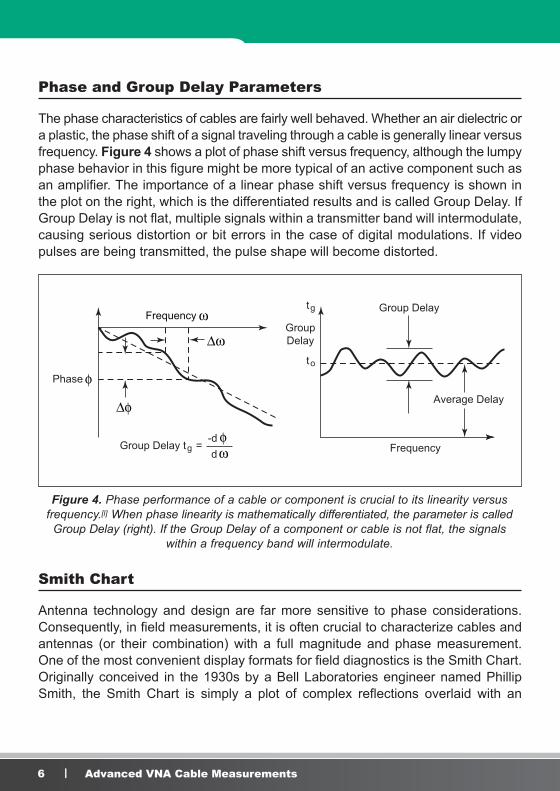
The phase characteristics of cables are fairly well behaved. Whether an air dielectric or a plastic, the phase shift of a signal traveling through a cable is generally linear versus frequency. Figure 4 shows a plot of phase shift versus frequency, although the lumpy phase behavior in this figure might be more typical of an active component such as an amplifier. The importance of a linear phase shift versus frequency is shown in the plot on the right, which is the differentiated results and is called Group Delay. If Group Delay is not flat, multiple signals within a transmitter band will intermodulate, causing serious distortion or bit errors in the case of digital modulations. If video pulses are being transmitted, the pulse shape will become distorted.

Smith Chart

Antenna technology and design are far more sensitive to phase considerations. Consequently, in field measurements, it is often crucial to characterize cables and antennas (or their combination) with a full magnitude and phase measurement. One of the most convenient display formats for field diagnostics is the Smith Chart. Originally conceived in the 1930s by a Bell Laboratories engineer named Phillip Smith, the Smith Chart is simply a plot of complex reflections overlaid with an

Frequency

φ

φ

∆φ

∆ω

ω

ω Frequency

Phase

Group Delay tg = -d

d

Group Delay

Average Delay

GroupDelay

tg

to

Figure 4. Phase performance of a cable or component is crucial to its linearity versus frequency.[l] When phase linearity is mathematically differentiated, the parameter is called Group Delay (right). If the Group Delay of a component or cable is not flat, the signals

within a frequency band will intermodulate.


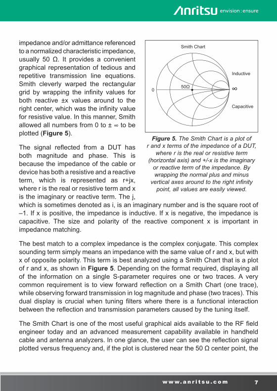
impedance and/or admittance referenced to a normalized characteristic impedance, usually 50 Ω. It provides a convenient graphical representation of tedious and repetitive transmission line equations. Smith cleverly warped the rectangular grid by wrapping the infinity values for both reactive ±x values around to the right center, which was the infinity value for resistive value. In this manner, Smith allowed all numbers from 0 to ± ∞ to be plotted (Figure 5).

The signal reflected from a DUT has both magnitude and phase. This is because the impedance of the cable or device has both a resistive and a reactive term, which is represented as r+jx, where r is the real or resistive term and x is the imaginary or reactive term. The j, which is sometimes denoted as i, is an imaginary number and is the square root of –1. If x is positive, the impedance is inductive. If x is negative, the impedance is capacitive. The size and polarity of the reactive component x is important in impedance matching.

The best match to a complex impedance is the complex conjugate. This complex sounding term simply means an impedance with the same value of r and x, but with x of opposite polarity. This term is best analyzed using a Smith Chart that is a plot of r and x, as shown in Figure 5. Depending on the format required, displaying all of the information on a single S-parameter requires one or two traces. A very common requirement is to view forward reflection on a Smith Chart (one trace), while observing forward transmission in log magnitude and phase (two traces). This dual display is crucial when tuning filters where there is a functional interaction between the reflection and transmission parameters caused by the tuning itself.

The Smith Chart is one of the most useful graphical aids available to the RF field engineer today and an advanced measurement capability available in handheld cable and antenna analyzers. In one glance, the user can see the reflection signal plotted versus frequency and, if the plot is clustered near the 50 Ω center point, the

50Ω

Smith Chart

Inductive

Capacitive

0 ∞

Figure 5. The Smith Chart is a plot of r and x terms of the impedance of a DUT,

where r is the real or resistive term (horizontal axis) and +/-x is the imaginary

or reactive term of the impedance. By wrapping the normal plus and minus

vertical axes around to the right infinity point, all values are easily viewed.


component is well matched. Using it, such problems can be solved in mere seconds, lessening the possibility of errors creeping into the calculations. Because Smith Chart graphically demonstrates how various RF parameters (e.g., impedances, reflection coefficients, S-parameters, noise figure circles, and gain contours) behave at one or more frequencies, it offers an alternative to using tabular information.

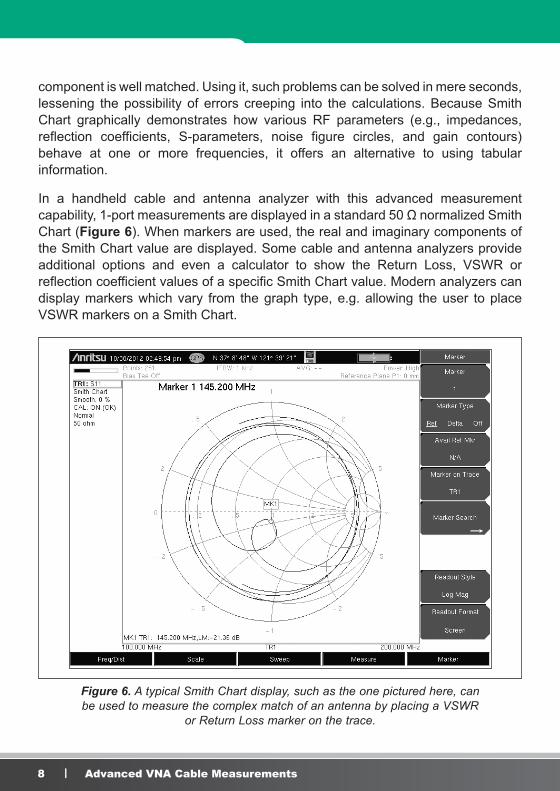
In a handheld cable and antenna analyzer with this advanced measurement capability, 1-port measurements are displayed in a standard 50 Ω normalized Smith Chart (Figure 6). When markers are used, the real and imaginary components of the Smith Chart value are displayed. Some cable and antenna analyzers provide additional options and even a calculator to show the Return Loss, VSWR or reflection coefficient values of a specific Smith Chart value. Modern analyzers can display markers which vary from the graph type, e.g. allowing the user to place VSWR markers on a Smith Chart.

Figure 6. A typical Smith Chart display, such as the one pictured here, can be used to measure the complex match of an antenna by placing a VSWR

or Return Loss marker on the trace.


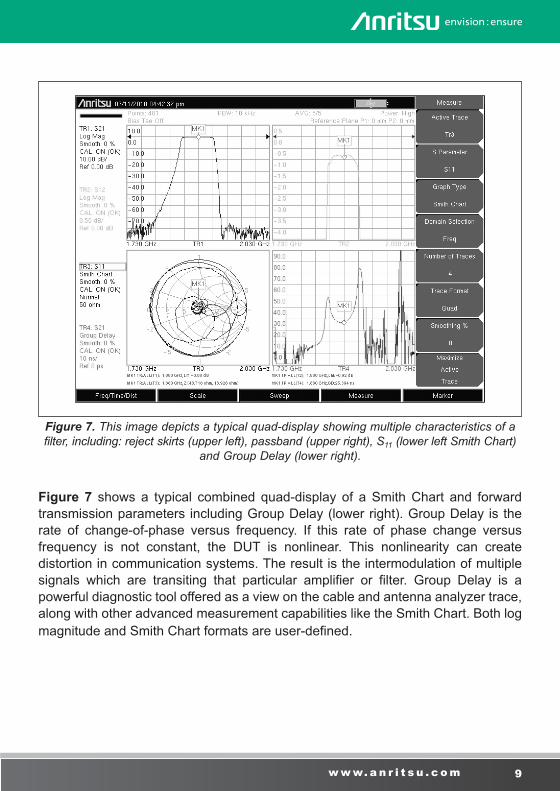
Figure 7 shows a typical combined quad-display of a Smith Chart and forward transmission parameters including Group Delay (lower right). Group Delay is the rate of change-of-phase versus frequency. If this rate of phase change versus frequency is not constant, the DUT is nonlinear. This nonlinearity can create distortion in communication systems. The result is the intermodulation of multiple signals which are transiting that particular amplifier or filter. Group Delay is a powerful diagnostic tool offered as a view on the cable and antenna analyzer trace, along with other advanced measurement capabilities like the Smith Chart. Both log magnitude and Smith Chart formats are user-defined.

Figure 7. This image depicts a typical quad-display showing multiple characteristics of a filter, including: reject skirts (upper left), passband (upper right), S11 (lower left Smith Chart)

and Group Delay (lower right).


Making Cable Phase Measurements in the Field

For measuring absolute insertion phase characteristics of a cable or comparing phase match between multiple RF/Microwave cables, especially in the field where access to AC power is limited, a portable VNA is the most appropriate tool. Some VNA models come with an optional built-in Vector Voltmeter (VVM) capability that enables a contractor, field technician or engineer to accurately measure or match the phase parameter in one or a multiple of cables with ease and high accuracy. A VNA with a VVM capability effectively replaces the functional ratio measurements of the now obsolete VVM and the signal generator.[1]

Many RF/Microwave systems depend on multiple antenna elements to create their transmitted beam, often with exceedingly precise requirements on the insertion phase or the phase match between the transmit cables. As an example, consider that precise directional characteristics are needed for the VHF Omnirange (VOR) navigation antenna systems at most airports. Detailed procedures are published for maintenance personnel to provide the exact phase match between cables. Glide slope antenna cables also require careful phase matching.

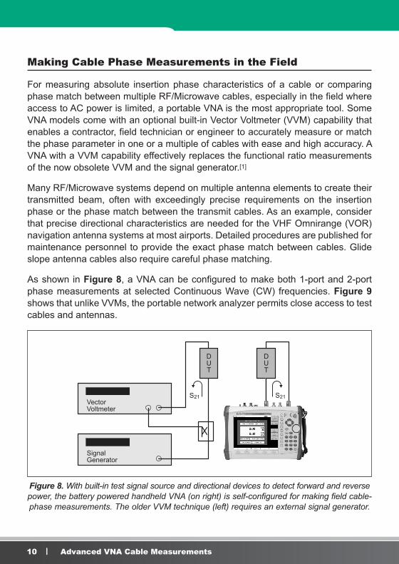
As shown in Figure 8, a VNA can be configured to make both 1-port and 2-port phase measurements at selected Continuous Wave (CW) frequencies. Figure 9 shows that unlike VVMs, the portable network analyzer permits close access to test cables and antennas.

VectorVoltmeter

SignalGenerator

DUT

DUT

S21 S21

Figure 8. With built-in test signal source and directional devices to detect forward and reverse power, the battery powered handheld VNA (on right) is self-configured for making field cable-phase measurements. The older VVM technique (left) requires an external signal generator.


Insertion and Reflection are two common techniques employed by the VNA to obtain cable-phase measurements. Both are based on S-parameters. The preferred method, Insertion, utilizes the VNA’s 2-port setup to make insertion phase measurements by measuring the S21 vector transmission from Port 1 to Port 2 through the cable. This allows the operator to determine the phase shift of the component or cable from its input connector to its output connector. Measured S21 data is displayed as cable insertion loss in dB, while insertion phase is displayed in degrees.

Reflection, on the other hand, measures the reflected signal S11 on a test cable, and is dependent on the far end of the cable being deliberately mismatched—either shorted or left as an open circuit. With the deliberate mismatch, virtually 100% of the input signal is reflected and as a result, the phase delay of the measured reflected signal is equal to twice the one-way phase of the cable. Similarly, the cable measured return loss is twice the one-way loss.

This reflection technique is especially useful in situations where the operator must manually create multiple phase-matched cables using the “measure-and-snip” operation. This operation requires the contractor, engineer or field technician to carefully snip small amounts of cable with a diagonal cutter, perhaps 1/8th inch at a time, and re-measure the effect on the 2-way phase. The reflection technique is also useful on already installed cables where the far end cannot be brought near the VNA instrument.

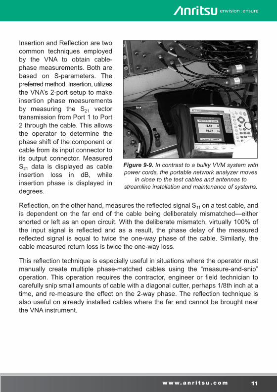
Figure 9-9. In contrast to a bulky VVM system with power cords, the portable network analyzer moves

in close to the test cables and antennas to streamline installation and maintenance of systems.


Two-Port Measurements

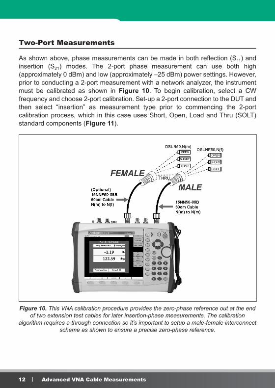
As shown above, phase measurements can be made in both reflection (S11) and insertion (S21) modes. The 2-port phase measurement can use both high (approximately 0 dBm) and low (approximately –25 dBm) power settings. However, prior to conducting a 2-port measurement with a network analyzer, the instrument must be calibrated as shown in Figure 10. To begin calibration, select a CW frequency and choose 2-port calibration. Set-up a 2-port connection to the DUT and then select “insertion” as measurement type prior to commencing the 2-port calibration process, which in this case uses Short, Open, Load and Thru (SOLT) standard components (Figure 11).

Figure 10. This VNA calibration procedure provides the zero-phase reference out at the end of two extension test cables for later insertion-phase measurements. The calibration

algorithm requires a through connection so it’s important to setup a male-female interconnect scheme as shown to ensure a precise zero-phase reference.


Note that when preparing system cables for precise match to other cables and the connectors of the cable under test are both the same gender (e.g., male-male), an extra female-female insert must be used in the calibration routine and its insertion effect on phase shift computed out of the final results.

For phase-matching cables, a good general practice is:

Step 1. Connectorize the first (reference) cable on both ends.

Step 2. Make an insertion phase measurement and store the data.

Step 3. Cut a second cable to length, being careful not to cut shorter than the reference cable, and connectorize it on both ends.

Step 4. Measure the second connectorized cable and compare it to the first (reference) cable.

From the difference observed, the user can estimate the trim required for the second cable. For more accurate trimming, one of the second cable’s connectors must be removed and the center conductor trimmed. Re-connect the connector back for another measured comparison with the first cable. Although, it may be difficult to trim the cable correctly the first time, experienced users often achieve success in the first two or three tries. However, this practice of measure-and-cut varies with frequency. Lower frequencies (VHF) will likely be in the 1/16th to 1/8th inch range for final iterations, while at 1 GHz and above, the re-connecting might only involve unsoldering the center conductor and trimming it 1/32 of an inch or less, and just letting the solder cool.

For example, at 118.5 MHz, 1.0 inch length of 1/4 inch diameter Andrew Heliax® with a phase velocity Vp = 0.84, equals approximately 4.28 degrees, while at 332.3 MHz, it equals 12.05 degrees. Often times, trimming the cable precisely for the last few tenths of a degree can be very exacting. Nevertheless, with careful and clever attention to detail and data, users can establish their own learning curve. The 2-port measurements taken appear on the analyzer’s display window as shown in Figure 12.

Figure 11. Convenient calibration components for the VNA provide the

Open, Short and Load standards for the SOLT calibration procedure.


One-Port Phase Measurements

The reflection or 1-port phase measurement is favored when one end of the cable cannot be brought up to the test instrument. Or, in cases where “measure-and-snip” operations must be performed to create cables of exactly the right phase length for a prescribed frequency. Prior to making these measurements, the VNA must be calibrated for 1-port measurements using the Open, Short, and Load setup shown in Figure 13.When using this technique to measure a cable’s phase length, it is assumed that the raw end of the cable reflects back 100% of the power. This condition is dependent on frequency. An open coaxial cable end will reflect virtually all of the power back at low frequencies (below 500 MHz), but might function as a non-efficient antenna at microwave frequencies. Thus, at higher frequencies the reflection is not complete. While in the VHF range, 100 to 500 MHz, an open end offers 100% reflection.

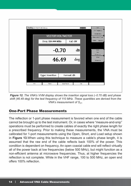
Figure 12. The VNA’s VVM display shows the insertion signal loss (–0.70 dB) and phase shift (46.49 deg) for the test frequency of 110 MHz. These quantities are derived from the

VNA’s measurement of S21.


Depending on the model, the VNA is capable of measurements up to 4, 6 or 20 GHz. At these higher microwave ranges, users are advised to prepare the cable center conductor and braided shield to be electrically shorted, such as by soldering the two together to ensure a good short. This extra soldering step complicates the “measure-and-snip” technique since once the required phase is obtained by multiple snips, the final addition of the real connector starts with a slightly damaged cable end. Nonetheless, with a little experience, the user will understand and adapt to the process.

While interactively measuring and snipping cables for matched phase may be a tedious job, it is made faster by experience. Two tips that can help with this task include:

Tip 1. At any one frequency, cut the cable to be prepared several inches longer than the final length. Solder the raw end, creating a good short and take a measurement. Next, cut off exactly one inch of cable, solder it identically again and take another measurement. Note the change in phase from the removal of the one inch segment

Figure 13. The reflection or 1-port phase measurement is the preferred procedure for cable measurements when both ends of the test cable cannot be brought to the

instrument. Prior to making these measurements, the VNA must be calibrated for 1-port measurements using the Open, Short and Load setup.


and calculate the amount of phase difference for, say, 1/8th inch. When the snip procedure brings you closer to the final desired value of the measured phase, you will have a good idea of how much more to snip.

Tip 2. Using the 1-port method, make a shorted-end phase measurement and note the value. Attach the final cable connector at that length using the normal connector attaching process. Next, make a 2-port connector-to-connector insertion phase measurement, as described above in Tip 1, and note the difference in phase. This correction value can be utilized in later steps when converting from the raw end measurements to the final connectorized configuration.

For comparing multiple cables for matched phase, the VNA can save measured phase and amplitude values of multiple cables in the memory of the portable cable and antenna analyzer as a convenient table. With this feature, the operator can save the first cable measurement as a reference, view the differences between the reference cable and other cables, and then output a final report showing both absolute and relative values of all cables. As an example, Figure 14 shows a

Figure 14. This screen capture displays results for multiple cables, showing both measured values of phase and amplitude for each cable. On the right is a typical soft key “Measurement Menu” cluster, showing the operator choices as the measurement progresses.


display table with measured values of phase and amplitude for each cable. Their relative phase and amplitude, with respect to a chosen “golden standard cable,” is shown in the top box as the REL standard.

Exploiting the Time-Domain Algorithm

For contractors, engineers and field technicians, the ability of time-domain analysis to separate impairments by time or distance is a powerful tool to analyze cables for faults. The instrument displays that provide DTF capture all the discontinuities that may occur due to a loose connection, corrosion, aging effects, or physical damage. This section will discuss special variations of Time-Domain measurements as applied to cable characterization, and distributed transmission elements where the ability to separate S-parameters by distance or time is a very valuable tool.[2]

Frequency Domain Reflectometry

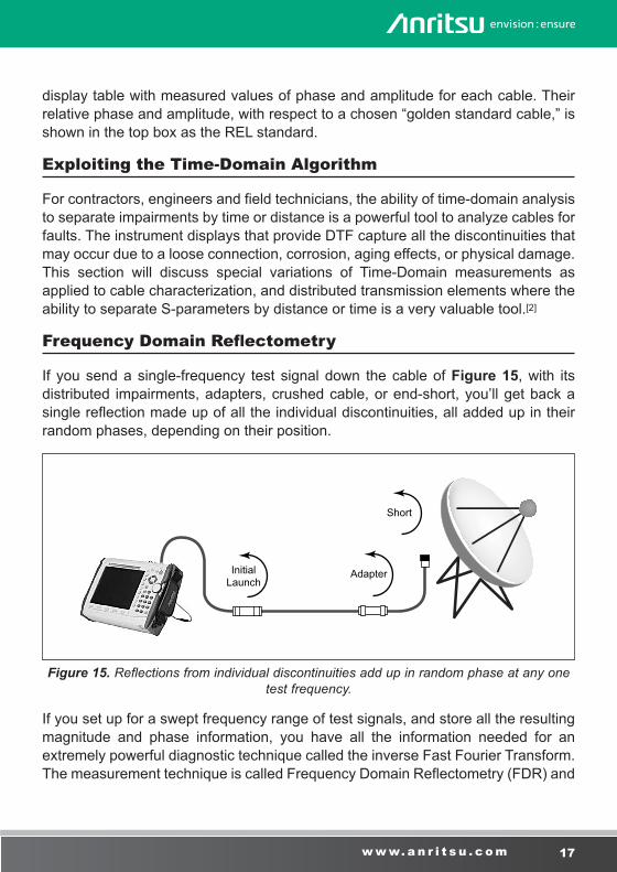
If you send a single-frequency test signal down the cable of Figure 15, with its distributed impairments, adapters, crushed cable, or end-short, you’ll get back a single reflection made up of all the individual discontinuities, all added up in their random phases, depending on their position.

If you set up for a swept frequency range of test signals, and store all the resulting magnitude and phase information, you have all the information needed for an extremely powerful diagnostic technique called the inverse Fast Fourier Transform. The measurement technique is called Frequency Domain Reflectometry (FDR) and

Short

AdapterInitialLaunch

Figure 15. Reflections from individual discontinuities add up in random phase at any one test frequency.


the VNA Master is configured to use operational frequencies (instead of DC-based pulses from the classic TDR approaches) to more precisely identify discontinuities. When access to both ends of the cable is convenient, a similar time-domain analysis is available on transmission (S21) measurements too.[3], [4]

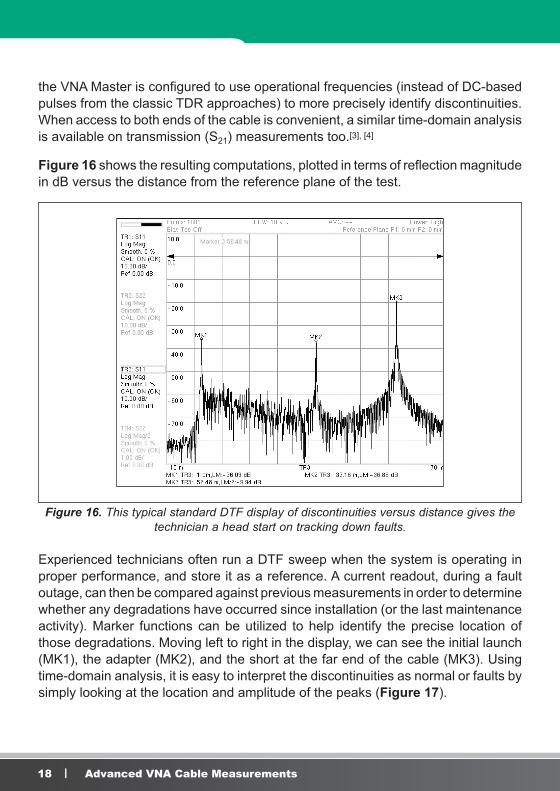
Figure 16 shows the resulting computations, plotted in terms of reflection magnitude in dB versus the distance from the reference plane of the test.

Experienced technicians often run a DTF sweep when the system is operating in proper performance, and store it as a reference. A current readout, during a fault outage, can then be compared against previous measurements in order to determine whether any degradations have occurred since installation (or the last maintenance activity). Marker functions can be utilized to help identify the precise location of those degradations. Moving left to right in the display, we can see the initial launch (MK1), the adapter (MK2), and the short at the far end of the cable (MK3). Using time-domain analysis, it is easy to interpret the discontinuities as normal or faults by simply looking at the location and amplitude of the peaks (Figure 17).

Figure 16. This typical standard DTF display of discontinuities versus distance gives the technician a head start on tracking down faults.


With the Time Domain Analysis (Option 0002), the VNA Master can also display the S-parameter measurements separated in the time or distance domain using this popular analysis mode. The broadband frequency coverage coupled with 4,001 data points means that you can measure discontinuities both near and far with unprecedented clarity for a handheld tool. With this option, you can simultaneously view S-parameters in frequency, time, and distance domain to quickly identify faults in the field.

Waveguide Transmission Lines

For microwave systems, with high power transmitters, the transmission line is often fabricated of waveguide. In the field, waveguide flanges can leak moisture and the condensation is a strong absorber. Also, the soft aluminum or brass waveguide is subject to physical damage in place. To handle waveguide lines in the field, the VNA Master also contains the mathematical functions which can compensate for the dispersion effect of the velocity of propagation in waveguide transmission lines.

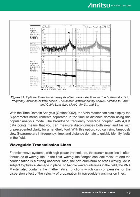
Figure 17. Optional time-domain analysis offers trace selections for the horizontal axis in frequency, distance or time scales. This screen simultaneously shows Distance-to-Fault

and Cable Loss (Log Mag/2) for S11 and S22.


One Way Versus Round Trip

With the ability to transform any S-parameter to the time domain, one question that arises is whether the time or distance that is plotted represents a one-way or a round-trip propagation. The one-way propagation represents the transmission (or 2-port) measurement, in which the signal is transmitted from one port, propagates through the DUT and is received on the second port. One-way propagation occurs when transforming S21 or S12.

The round-trip propagation represents a reflection (1-port) measurement, in which the signal is transmitted from one port, propagates through the DUT, fully reflects at the end of the device, and is received back at the same port. One-way propagation occurs when transforming S11 or S22.

The VNA Master handles one-way and round-trip propagation differently in the time and distance domains. In the time domain, the VNA Master plots the response against the actual time the signal travels from the transmission port to the receiving port without accounting for whether the measurement is transmission (2-port) or reflection (1-port). In the distance domain, however, the VNA Master compensates for the round-trip propagation by showing the actual length of the DUT (essentially dividing the distance by 2 for the reflection measurements).

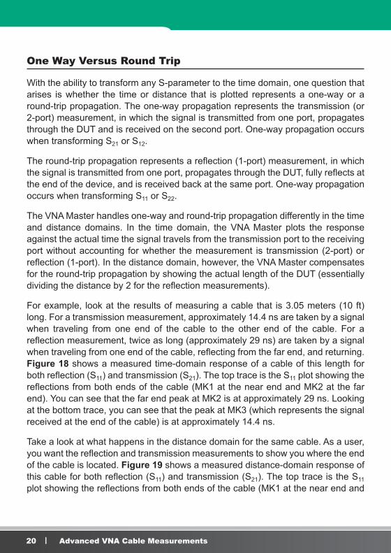
For example, look at the results of measuring a cable that is 3.05 meters (10 ft) long. For a transmission measurement, approximately 14.4 ns are taken by a signal when traveling from one end of the cable to the other end of the cable. For a reflection measurement, twice as long (approximately 29 ns) are taken by a signal when traveling from one end of the cable, reflecting from the far end, and returning. Figure 18 shows a measured time-domain response of a cable of this length for both reflection (S11) and transmission (S21). The top trace is the S11 plot showing the reflections from both ends of the cable (MK1 at the near end and MK2 at the far end). You can see that the far end peak at MK2 is at approximately 29 ns. Looking at the bottom trace, you can see that the peak at MK3 (which represents the signal received at the end of the cable) is at approximately 14.4 ns.

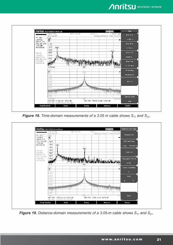
Take a look at what happens in the distance domain for the same cable. As a user, you want the reflection and transmission measurements to show you where the end of the cable is located. Figure 19 shows a measured distance-domain response of this cable for both reflection (S11) and transmission (S21). The top trace is the S11 plot showing the reflections from both ends of the cable (MK1 at the near end and


Figure 18. Time-domain measurements of a 3.05 m cable shows S11 and S21.

Figure 19. Distance-domain measurements of a 3.05-m cable shows S11 and S21.


MK2 at the far end). The bottom trace shows the transmission S21 measurement with the peak representing the signal received at the end of the cable (MK3). Looking at the signal at MK2 and MK3, you can see that the reflection and transmission measurements produced the same result for the length of the cable. The VNA Master compensated for the round-trip condition in the S11 measurement so that the distance information matches the physical length of the cable, just as it does in the S21 measurement.

Note that the measured cable had a propagation velocity of 70%, which was entered into the VNA Master. Measurements in the distance domain use the entered propagation velocity value to calculate the actual physical length of cables. If the default value of 100% were used, then the measured cable length would be wrong (4.4 meters in the above example). Time-domain measurements are not dependent on the propagation velocity values.

Gated Time Domain

Gating is a popular technique for further analyzing discontinuities observed in the time domain. In the most popular scenario, one would highlight a desired discontinuity with a gate consisting of start and stop criteria. Once selected and enabled, the gate modifies measurements to show only the effect of the gate from start to stop in the swept frequency display. As an alternative, the gate can be configured as a notch to remove the effect of the gated portion from the current measurement. For closely spaced discontinuities, additional filtering options are provided to control how the gate is applied to further optimize the current measurement.

Anti-aliasing is an important consideration for time-domain analysis to ensure adequate distance/time is available for viewing discontinuities. For improved distance resolution, closely spaced discontinuities may require greater frequency spans. For greater maximum distance, more data points or narrower frequency spans will increase the maximum alias-free viewable distance (e.g., Dmax). For more setup information, refer to Chapter 4 on measurement aids.

Measurement Readout and Interpretation

When gating is enabled, the trace readout in frequency domain is labeled with Frequency Gated with Time (FGT) to differentiate this applied post-processing from normal measurements. Verifying deployed cable is operating properly usually requires, at a minimum, the measurement of Cable Loss and Return Loss. In this


typical field scenario, the far end of the cable is disconnected from the antenna and replaced by calibration devices: open/short for Cable Loss and load/termination for Return Loss. The following example shows how to use the new gating features to observe Cable Loss and Return Loss with a single connection.

Setup Considerations

Let’s start by configuring the instrument to show Cable Loss and Return Loss on a single display. As a setup step, calibrate the instrument at Port 1 for 1-port measurements between 1 GHz and 2 GHz with 201 data points. Two traces are setup with S11 log magnitude displays as their assigned S-parameter: trace 1 (TR1) is Return Loss and trace 2 (TR2) is Cable Loss (e.g., Log Mag/2 graph type).

Following the 1-port calibration, we connect two 1.5 m cables in series, representing the DUT with propagation velocity (vp) of 0.7 for the sequence of measurements that follow.

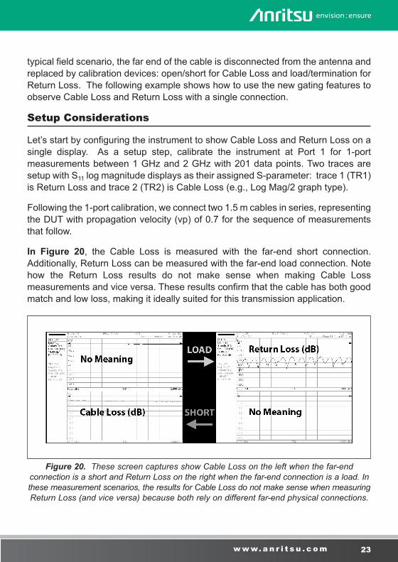
In Figure 20, the Cable Loss is measured with the far-end short connection. Additionally, Return Loss can be measured with the far-end load connection. Note how the Return Loss results do not make sense when making Cable Loss measurements and vice versa. These results confirm that the cable has both good match and low loss, making it ideally suited for this transmission application.

Figure 20. These screen captures show Cable Loss on the left when the far-end connection is a short and Return Loss on the right when the far-end connection is a load. In these measurement scenarios, the results for Cable Loss do not make sense when measuring Return Loss (and vice versa) because both rely on different far-end physical connections.


Gate Setup to Simultaneously Measure Cable Loss and Return Loss

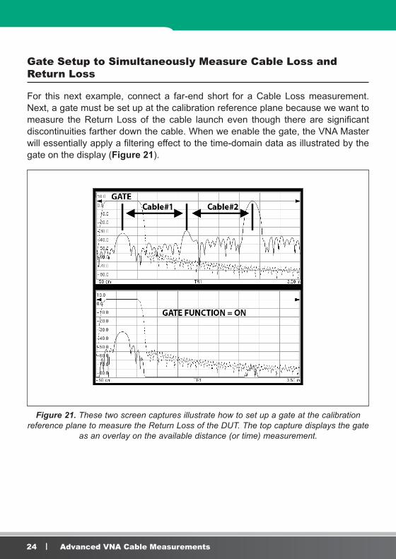
For this next example, connect a far-end short for a Cable Loss measurement. Next, a gate must be set up at the calibration reference plane because we want to measure the Return Loss of the cable launch even though there are significant discontinuities farther down the cable. When we enable the gate, the VNA Master will essentially apply a filtering effect to the time-domain data as illustrated by the gate on the display (Figure 21).

Figure 21. These two screen captures illustrate how to set up a gate at the calibration reference plane to measure the Return Loss of the DUT. The top capture displays the gate

as an overlay on the available distance (or time) measurement.


FGT Reveals Return Loss and Cable Loss

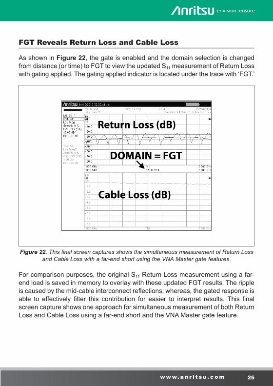
As shown in Figure 22, the gate is enabled and the domain selection is changed from distance (or time) to FGT to view the updated S11 measurement of Return Loss with gating applied. The gating applied indicator is located under the trace with ‘FGT.’

For comparison purposes, the original S11 Return Loss measurement using a far-end load is saved in memory to overlay with these updated FGT results. The ripple is caused by the mid-cable interconnect reflections; whereas, the gated response is able to effectively filter this contribution for easier to interpret results. This final screen capture shows one approach for simultaneous measurement of both Return Loss and Cable Loss using a far-end short and the VNA Master gate feature.

Figure 22. This final screen captures shows the simultaneous measurement of Return Loss and Cable Loss with a far-end short using the VNA Master gate features.


Gate Shape: Minimal, Nominal, Wide, and Maximum

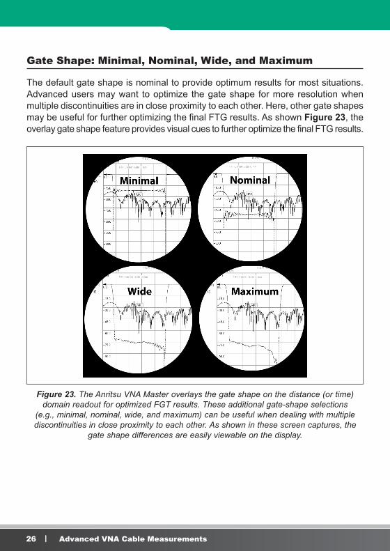
The default gate shape is nominal to provide optimum results for most situations. Advanced users may want to optimize the gate shape for more resolution when multiple discontinuities are in close proximity to each other. Here, other gate shapes may be useful for further optimizing the final FTG results. As shown Figure 23, the overlay gate shape feature provides visual cues to further optimize the final FTG results.

Figure 23. The Anritsu VNA Master overlays the gate shape on the distance (or time) domain readout for optimized FGT results. These additional gate-shape selections

(e.g., minimal, nominal, wide, and maximum) can be useful when dealing with multiple discontinuities in close proximity to each other. As shown in these screen captures, the

gate shape differences are easily viewable on the display.


Time Domain Diagnostics for Balanced/Differential Transmission Lines

Modern digital communications systems utilize pulse rates in the 10 Gbps range. Such pulses require frequency-response bandwidths of 25 GHz and more. When those extremely high data rate signals are to be cabled from one sub-system rack to another, simple shielded twisted pair wiring will not do. Yet, the signals must be designed to be immune to noise pickup. This leads system designers to specify balanced or differential coaxial transmission lines. The digital data stream is contained between the two center conductors of regular coaxial transmission lines. The terminology for the S11 parameter for such differential line set is Sd1d1.

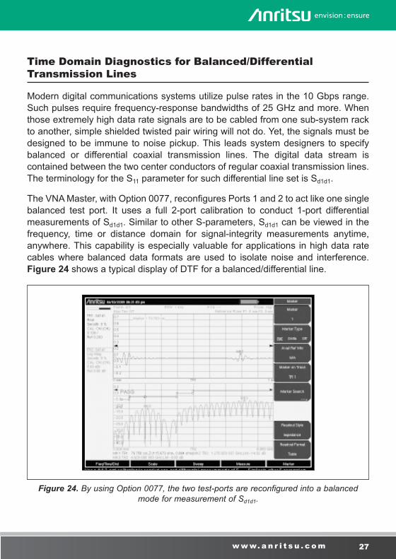
The VNA Master, with Option 0077, reconfigures Ports 1 and 2 to act like one single balanced test port. It uses a full 2-port calibration to conduct 1-port differential measurements of Sd1d1. Similar to other S-parameters, Sd1d1 can be viewed in the frequency, time or distance domain for signal-integrity measurements anytime, anywhere. This capability is especially valuable for applications in high data rate cables where balanced data formats are used to isolate noise and interference. Figure 24 shows a typical display of DTF for a balanced/differential line.

Figure 24. By using Option 0077, the two test-ports are reconfigured into a balanced mode for measurement of Sd1d1.


Time Domain Separation of S-Parameters

While not strictly a cable or antenna characterization, the following tuning procedures for highly-complex passband filters demonstrates the powerful ability of the Time Domain function to separate the S-parameters of a DUT in distance or time.[5] In the quest for superior filter performance, and the ability to create specific filter specifications, filter designers now utilize extremely complex architectures. This makes manufacturing and final test a difficult endeavor, not to mention the challenges associated with the field servicing requirement.

In this case, a number of different resonators can be used; lumped LC circuits are good for production on printed circuit type technology. Cavity resonators are good for high power. Waveguide models have used “waffle iron” type machining to develop filtering. Dielectric resonators tend to have higher Q factors. Producing more sophisticated filter parameters, sharper skirts and flatter passbands, multiple “poles” or resonators need to be used. Suppose you use 5 resonators designed to “cross-couple” certain individual effects, multiplying their features and producing sharper rejection skirts and deeper stop bands. Flat passbands are still maintained with the desired flat Group Delay.

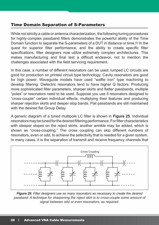
A generic diagram of a tuned multipole LC filter is shown in Figure 25. Individual resonators may be tuned for the desired filtering performance. For filter characteristics with steeper slopes on the reject skirts, another wrinkle may be added, which is shown as “cross-coupling.” The cross coupling can skip different numbers of resonators, even or odd, to achieve the selectivity that is needed for a given system. In many cases, it is the separation of transmit and receive frequency channels that

Cross Coupling

Figure 25. Filter designers use as many resonators as necessary to create the desired passband. A technique for sharpening the reject skirt is to cross-couple some amount of

signal between odd or even resonators, as required.


determines the specific design. Since the resonators are physically distributed, the VNA Master’s Time-Domain function can be used to display the tuning effect of each resonator individually.

While in general, the more poles or tunable resonant circuits used, the better the flatness, this is not completely true. More resonances also mean more loss across the passband, so practical filters might be 5 or 8 poles. But in the tuning stages, if the only measurement instrument shows a frequency versus attenuation plot, the tuning situation can be hopeless because of the extreme interaction between almost all tuning screwdriver slots.

One measurement answer is the ability to electronically separate the display of individual resonators by their physical position. This can be done with a powerful time-domain feature found in modern VNAs. Figure 26 shows a typical measurement display where the time domain separation assists in tuning bandpass characteristics.

Figure 26. Powerful insights are now available with time-domain measurements of multiple resonator filters. This screen shot shows two views of S21 passband, one with 0.5 dB and

the other 5.0 dB per division. The bottom trace shows the time-domain separated views of individual resonators, allowing the filter tuner person to have a better idea of what the

tuning is doing.


On the top overlay, two versions of the passband S21 are overlaid, one being 0.5 dB per division and the other (showing sharp skirts) is 5.0 dB per division. The lower display shows attenuation for the various resonators, separated by distance, with the markers MK1 and MK2 designating their physical distance.

Finally, it should be noted that the Time Domain option for VNAs is not the traditional nanosecond-pulses-down-a-coaxial line of oscilloscope TDRs. Instead it is based on the use of a FDR technique, which captures data over a band-limited range of frequencies, and uses powerful inverse-Fourier transform data processing to develop and display a time separated view of transmission or reflection. The use of band-limited data also means it is also useful for waveguide lines which are band-limited by definition.

Summary

The insight and diagnostic power that the handheld VNA brings to field test and maintenance is stunning. For all the simple routines of characterizing components, cables and antennas, its accuracy and speed is expected. But, for the complex and sophisticated test routines of Time Domain and Precision Phase measurements, the specialized options of the VNA are crucial. Although not discussed herein, the ability of the contractor, field technician or engineer to add a powerful spectrum analyzer to the basic VNA takes a brand new test system on the road, anytime, anywhere.


References

1. Practical Tips on Making “Vector Voltmeter (VVM)” Phase Measurements using VNA Master (Opt 15), Anritsu Application Note 11410-00531.

2. Distance to Fault, Anritsu Application Note 11410-00373.

3. Reflectometer Measurements—Revisited, Anritsu Application Note 11410-00214.

4. Time Domain Measurements Using Vector Network Analyzers, Anritsu Application Note 11410-00206.z

5. Primer on Vector Network Analysis 11410-00387.

• United States Anritsu Company1155 East Collins Boulevard, Suite 100, Richardson, TX, 75081 U.S.A. Toll Free: 1-800-267-4878 Phone: +1-972-644-1777 Fax: +1-972-671-1877

• Canada Anritsu Electronics Ltd.700 Silver Seven Road, Suite 120, Kanata, Ontario K2V 1C3, Canada Phone: +1-613-591-2003 Fax: +1-613-591-1006

• Brazil Anritsu Electrônica Ltda.Praça Amadeu Amaral, 27 - 1 Andar 01327-010 - Bela Vista - Sao Paulo - SP - Brazil Phone: +55-11-3283-2511 Fax: +55-11-3288-6940

• Mexico Anritsu Company, S.A. de C.V.Av. Ejército Nacional No. 579 Piso 9, Col. Granada 11520 México, D.F., México Phone: +52-55-1101-2370 Fax: +52-55-5254-3147

• United Kingdom Anritsu EMEA Ltd.200 Capability Green, Luton, Bedfordshire LU1 3LU, U.K. Phone: +44-1582-433280 Fax: +44-1582-731303

• France Anritsu S.A.12 avenue du Québec, Batiment Iris 1-Silic 612, 91140 Villebon-sur-Yvette, France Phone: +33-1-60-92-15-50 Fax: +33-1-64-46-10-65

• Germany Anritsu GmbHNemetschek Haus, Konrad-Zuse-Platz 1 81829 München, Germany Phone: +49-89-442308-0 Fax: +49-89-442308-55

• Italy Anritsu S.r.l.Via Elio Vittorini 129, 00144 Roma Italy Phone: +39-06-509-9711 Fax: +39-06-502-2425

• Sweden Anritsu ABKistagången 20B, 164 40 KISTA, Sweden Phone: +46-8-534-707-00 Fax: +46-8-534-707-30

• Finland Anritsu ABTeknobulevardi 3-5, FI-01530 VANTAA, Finland Phone: +358-20-741-8100 Fax: +358-20-741-8111

• Denmark Anritsu A/SKay Fiskers Plads 9, 2300 Copenhagen S, Denmark Phone: +45-7211-2200 Fax: +45-7211-2210

• Russia Anritsu EMEA Ltd. Representation Office in RussiaTverskaya str. 16/2, bld. 1, 7th floor. Moscow, 125009, Russia Phone: +7-495-363-1694 Fax: +7-495-935-8962

• Spain Anritsu EMEA Ltd. Representation Office in SpainEdificio Cuzco IV, Po. de la Castellana, 141, Pta. 5 28046, Madrid, Spain Phone: +34-915-726-761 Fax: +34-915-726-621

• United Arab Emirates Anritsu EMEA Ltd. Dubai Liaison OfficeP O Box 500413 - Dubai Internet City Al Thuraya Building, Tower 1, Suite 701, 7th floor Dubai, United Arab Emirates Phone: +971-4-3670352 Fax: +971-4-3688460

• India Anritsu India Pvt Ltd.2nd & 3rd Floor, #837/1, Binnamangla 1st Stage, Indiranagar, 100ft Road, Bangalore - 560038, India Phone: +91-80-4058-1300 Fax: +91-80-4058-1301

• Singapore Anritsu Pte. Ltd.11 Chang Charn Road, #04-01, Shriro House Singapore 159640 Phone: +65-6282-2400 Fax: +65-6282-2533

• P. R. China (Shanghai) Anritsu (China) Co., Ltd.27th Floor, Tower A, New Caohejing International Business Center No. 391 Gui Ping Road Shanghai, Xu Hui Di District, Shanghai 200233, P.R. China Phone: +86-21-6237-0898 Fax: +86-21-6237-0899

• P. R. China (Hong Kong) Anritsu Company Ltd.Unit 1006-7, 10/F., Greenfield Tower, Concordia Plaza, No. 1 Science Museum Road, Tsim Sha Tsui East, Kowloon, Hong Kong, P. R. China Phone: +852-2301-4980 Fax: +852-2301-3545

• Japan Anritsu Corporation8-5, Tamura-cho, Atsugi-shi, Kanagawa, 243-0016 Japan Phone: +81-46-296-6509 Fax: +81-46-225-8352

• Korea Anritsu Corporation, Ltd.5FL, 235 Pangyoyeok-ro, Bundang-gu, Seongnam-si, Gyeonggi-do, 13494 Korea Phone: +82-31-696-7750 Fax: +82-31-696-7751

• Australia Anritsu Pty Ltd.Unit 20, 21-35 Ricketts Road, Mount Waverley, Victoria 3149, Australia Phone: +61-3-9558-8177 Fax: +61-3-9558-8255

• Taiwan Anritsu Company Inc.7F, No. 316, Sec. 1, Neihu Rd., Taipei 114, Taiwan Phone: +886-2-8751-1816 Fax: +886-2-8751-1817

Part No. 11410-00685, Rev. B Printed in United States 2017-07©2017 Anritsu Company. All Rights Reserved

® Anritsu All trademarks are registered trademarks of their respective companies. Data subject to change without notice. For the most recent specifications visit: www.anritsu.com

Specifications are subject to change without notice.

Advanced VNA Cable Measurements Product Brief...4 | Advanced VNA Cable Measurements VNA Fundamentals...

Documents

Transcript of Advanced VNA Cable Measurements Product Brief...4 | Advanced VNA Cable Measurements VNA Fundamentals...