Advanced Planning & Scheduling (APS)

The acronym APS or Advanced Planning & Scheduling originated with the Advanced Manufacturing Research (AMR) in the early 1990s.

It was created because a new breed of software was becoming available that failed the traditional ERP & MES litmus test.

A few hallmarks of an APS system usually include:

– Fewer internal users than ERP systems

– The use of memory resident models in addition to traditional data base management systems.

– Advanced planning & scheduling functionality

– Advanced optimization algorithms such as linear programming and other heuristics.

– Planning at a finer time increment

– Ability to do rapid what-if simulation

– Advanced problem notification

APS Software Solution Providers

There are only a few significant companies providing APS software solution. However, this number is expected to grow in the future.

Major APS software providers are:

– SAP

– i2 Technologies

– Manugistics

– Oracle (up and coming)

– Plus others

SAP APO

The SAP APO application is SAP’s version of Advanced Planning & Scheduling.

APO is bundled with several other advanced planning applications into mySAP SCM 5.0.

– Advanced Planning & Optimization (APO)

– Forecasting and Replenishment – Retail

– Inventory Collaboration Hub

– Event Manager

– Extended Warehouse Management

MySAP SCM

APO Architecture

APO Architecture

Legend:BW=BusinessWarehouseATP=GlobalAvailable-To-PromiseDP=DemandPlanningLC=Live CacheOB=MasterData ObjectsSNP=SupplyNetworkPlanningRDB=RelationalData BaseCIF=CoreInterface

System Definition (provided by UCC)

YOU WILL NEEDTO CREATE A NEW ENTRY INTO YOUR SAP GUI

System Definition (provided by UCC)

Data Flows

APO Demand Planning (DP)

APO Demand Planning (DP) is used to create a forecast of market demand for your company's products.

DP allows you to take into consideration the many different causal factors that affect demand.

DP contains a large library of statistical forecasting models.

Customers may also develop unique forecasting models using a powerful macro tool.

Forecasts created by APO DP may be released to APO Supply Network Planning or passed to R/3 for MRP planning.

APO Supply Network Planning (SNP)

APO Supply Network Planning (SNP) integrates purchasing, manufacturing, distribution, and transportation so that a comprehensive tactical planning and sourcing decisions can be simulated and implemented on the basis of a single, global consistent model.

Starting from a demand plan, Supply Network Planning creates a medium-term, rough-cut plan for fulfilling the estimated sales volumes.

Supply Network Planning uses advanced optimization techniques, based on constraints and penalties, to plan product flow along the supply chain

APO Production Planning/Detail Scheduling (PP/DS)

APO Production Planning/Detailed Scheduling (PP/DS) is intended to be a short-term (1-6 weeks), detailed planning and scheduling tool.

The PP portion of PP/DS is capable of creating finite supply chain plans taking capacities into consideration.

The DS portion of PP/DS is capable of creating optimized scheduling sequences

PP/DS accomplishes it primary mission by using various advanced heuristic and linear programming algorithyms.

APO Global Available To Promise (GATP)

Global Available To Promise (GATP) is an advanced order promising tool.

It extends the Available-To-Promise capability currently in SAP R/3 to include:

– Multiple plant planning

– Simulation of orders (Capable-To-Promise)

– Rule-based order promising

APO Transportation Planning/Vehicle Scheduling (TP/VS)

Transportation Planning/Vehicle Scheduling is intended to optimize the planning and schedule inbound and outbound freight.

The Transportation Planning portion of TP/VS enables you to make optimal use of the available capacity of trucks, trains, ships, and airplanes.

The Vehicle Scheduling component of TP/VS will optimize the delivery routes.

TP/VS utilizes advanced linear programming algorithms to accomplish its mission.

APO Alert Monitor

The Alert Monitor is an advanced monitoring system to detect supply chain problems at the earliest possible time.

The Alert Monitor is capable of operating within all the APO sub-modules (DP, SNP, PPS/DS, TP/VS).

Alert conditions may customized by company or individual user.

APO Alert Monitor

Introduction To CIF

The APO Core Interface framework (CIF) is used for the data exchange between SAP APO and SAP R/3 Systems.

The CIF will transfer both master data and transaction data from SAP R/3 to SAP APO and also from SAP APO to SAP R/3.

Data passing between SAP R/3 and SAP APO may be either real-time or batched.

The IT technology used for the interface is the Remote Function Call (RFC).

The passing of data is enabled by the creation and maintenance of Integration Models.

All Integration Models are defined in SAP R/3 (host system)

CIF Architecture

Integration With Multiple R/3 Systems

Master Data Transfer Through CIF

Transaction Data Transfer Through CIF

Integration Models

Multiple integration models will be used in connecting SAP R/3 to APO. Each model will transfer different data.

– Example – an integration model will be defined for transferring the organizational data elements (plant, storage locations, etc) to APO.

Integration models are always defined in the SAP R/3 system.

Various definitions must be made in configuration in both R/3 and APO.

R/3 and APO contain various tools for monitoring and handling integration errors.

Integration Model Example

Master Data Maintenance

Master data that was originated in SAP R/3 IS MAINTAINED IN R/3

Master data that is unique to APO IS MAINTAINED IN APO.

Selecting APO Planned Materials

Models In APO

All Master Data transferred using the CIF is automatically assigned to model 000 (Active model) in live cache.

Therefore models in APO contain master data.

Since APO may be used for simulation or what-if planning, other models may be created that contain master data different from the model 000 (active model).

Versions In APO

All transaction data that is transferred to APO through the CIF is stored in Version 000 (Active Version).

Examples of transaction data would be forecasts, sales orders, etc.

Since APO may be used for simulation or what-if purposes, other versions may be created that contain transaction data different from Version 000 (active version).

All transaction data transferring from APO to R/3 must be stored in Version 000.

Models & Versions In APO

Aaa

The University of Texas at Dallas© 2005 by SAP AG. All rights reserved.

13

Models & Versions In APO

What-IfModel

Versions containTransaction data

Models containMaster data

APO Master Data

The Master Data Objects in SAP APO have different names from their SAP R/3 counterparts. For example, the Material Master in R/3 is named Product Master in APO.

Many of the APO master data fields originate in R/3 and are transferred through the Core Interface (CIF).

APO has many other master data fields that do not have counterparts in R/3. These master data fields are needed to perform the APS functionality that does not exist in R/3.

APO also has one master data objects that does not have a R/3 counterpart.

Master data is maintained in its system of origin. R/3 fields in R/3 and APO fields in APO.

APO Master Data

Location Master

The Location Master is a common master data object used to house the following R/3 objects:

– Plant

– Customer

– Supplier

– Plus others

The University of Texas at Dallas© 2005 by SAP AG. All rights reserved.

APO Master Data

Quota Arrangement

Transportation Lane

Procurement Relationship

Purchasing Info Record

Scheduling Agreement

The location master is crucial to supply chain management because it is the building block for so many other relationships.

Location Master

Location Master Example

Transportation Lane

The APO Transportation Lane (TL) does not have a R/3 counterpart.

The TL defines all valid transportation method between two locations.

TLs may be defined for all products moved between two locations or may be specific by product.

If no TL exists between two locations then one location cannot be a source of supply to the other.

The TL may define multiple valid transportation means (truck, rail, air) along with the transportation time and cost for each.

APO sourcing algorithms will examine the TL for cost and time data to determine the optimum method.

Transportation Lane Example

Quota Arrangement

The quota arrangement determines the source and quantity demanded when several possible suppliers (i.e. locations) are available.

Quota arrangements exist in R/3 BUT ARE NOT USED IN APO.

Quota arrangements may be defined for all products sourced from a location or it may be product specific.

Product splits may be defined as:

– Fixed split

– Determined by a heuristic algorithm

– Determined optimally and then remain fixed.

If there is only 1 source of supply than no quota arrangement is needed.

Quota Arrangement Example

Product Master

The APO Product Master is the direct equivalent of the R/3 Material Master.

Most of the data from the MRP data views will pass through the Core Interface to create the Product Master.

The Product Master will also contain data elements that do not exist in R/3. A few examples are:

– Penalty costs – these reflect the relative cost of missing an order due date.

– Storage costs – the relative cost of storing a product.

– Good receipt/issue costs.

These costs are used to influence the Optimizer program in Supply Network Planning.

Product Master

Product Master

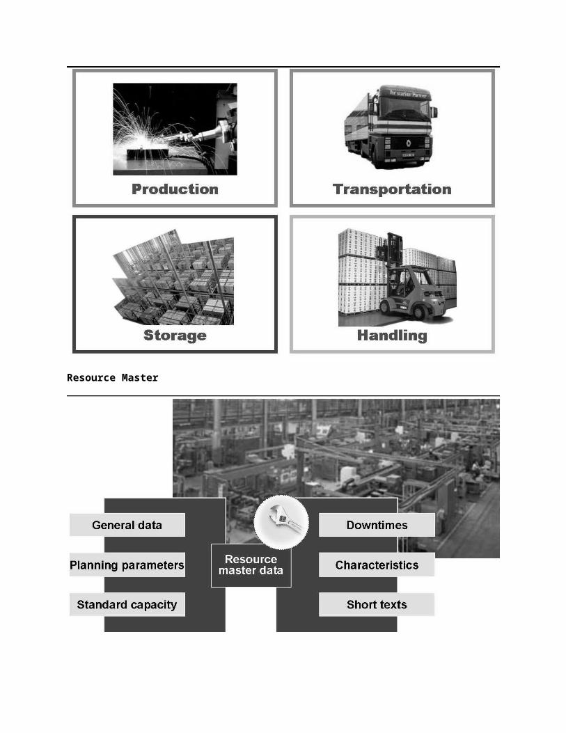
Resource Master

The APO Resource Master is the direct equivalent of the R/3 Work Center (discrete) or Resource (process).

The APO Resource Master is considerably more flexible than its R/3 counterparts. For example, in R/3 a work center may have multiple capacities (labor and machine).

When used in a APO environment, each capacity will create a separate and distinct resource. This allows for capacity planning for both resources.

Finally, the APO Resource may be used to model transportation and material handling resources.

Resources in APO may be Model/Version dependent for what-if simulation purposes.

Resource Master

Resource Master

Resource Master Example

Production Process Model (PPM)

The APO PPM is a complicated and sophisticated object that combines the major components of the R/3 BOM and Routing.

There the PPM will contain all the materials required and all the process steps, resources and processing times.

Additionally the PPM may also contain production cost data. This allows for PPMs to be created for various locations (plants) with different production costs. A linear programming sourcing model may then determine the optimum quantity to source from each location.

Two Types of PPMs

PPM Example

Procurement Relationship

The APO Procurement Relationship object is the direct equivalent of the R/3 Purchasing Information Record, Contract or Scheduling Agreement.

Since all of these R/3 objects define a valid relationship between a supplier and a trading partner the Core Interface will automatically create a Transportation Lane.

Procurement Relationship Example

Forecasting Basics

A forecast is a prediction of a variable of interest for a future time period.

The three absolutes of forecasting are:

– Forecasts are always wrong

– Forecasts are more accurate in groups rather than individuals

– Forecasts are more accurate in the near term

Forecasting techniques in SAP are:

– Manual

– Sales & Operations Planning (SOP)

– Flexible Planning (R/3)

– APO Demand Planning

Forecast Generation Methods

Forecast are almost always generated at a product family level as a background job that runs automatically.

Various organizations may make independent forecasts. Examples may include: sales, marketing, finance, and operations management.

The frequency of running the forecast will vary from company and industry. However, a monthly update frequency is the most common.

For each forecast cycle some time periods will be re-forecasted and some time periods will be forecasted for the 1st time. The overall horizon of the forecast is dependent upon several factors including:

– 1. Purpose of forecast

– 2. Cumulative product lead time

The forecast cycle may terminate with a consensus forecast as part of a Sales & Operations Planning (S&OP) meeting.

When the automatic forecast is completed, any alert conditions are noted and sent to customers.

Adjustments to automatic forecast are usually performed manually.

Typical Industry Forecasting Process

Approaches to Forecasting

Qualitative Method subjective inputs

– Subjective inputs

• “Soft” information (human factors, personal opinion, hunch)

• Hard to quantify

Quantitative Method objective, or hard, data

– Projection of historical data

– Associative models utilizing explanatory variables

Types of Forecasts

Qualitative

Judgmental - uses subjective inputs(consumer surveys, sales staff, managers/executives, expert panels)

Quantitative

Time series - uses historical data assuming the future will be like the past

Associative models - uses explanatory variables to predict the future

Time Series Forecasts

Time series – time-ordered sequence of observations taken at regular intervals

– Assume future can be estimated by past

– Identify underlying behavior without identifying causes

Time Series Forecasts

Trend – long-term upward/downward movement in data

Seasonality – short-term regular variations in data

Cycle – wavelike variations of more than one year’s duration

Irregular variations – caused by unusual circumstances

Random variations – caused by chance…what’s left

Forecast Variations

trend, seasonality, cycle, irregular variation, randomness

Techniques for Averaging

Historical data has “white noise or variation”

Averages smooth variations

3 Techniques

– Moving average

– Weighted moving average

– Exponential smoothing

Moving Averages

Technique that averages a number of recent actual values, updated as new values become available

Simple Moving Average

Weighted Moving Averages

Weighted moving average – more recent values in a series are given more weight in computing the forecast

Exponential Smoothing

Weighted averaging method based on previous forecast plus a percentage of the forecast error

WHERE ALPHA (SMOOTHING FACTOR) IS GREATER THAN OR EQUAL TO ZERO BUT LESS THAN OR

EQUAL TO 1

Example: Exponential Smoothing

Picking a Smoothing Constant

Forecast Evaluation

Forecast Errors

All error measures compare the forecast model to the actual data for the ExPost Forecast region

Errors Measure

t F(t) A(t)Error

F(t) - A(t) | F(t) - A(t) |25 95 91 4 426 125 137 -12 1227 197 193 4 428 227 199 28 2829 230 278 -48 4830 274 344 -70 7031 274 291 -17 1732 255 250 5 533 244 171 73 7334 211 152 59 5935 114 111 3 336 85 127 -42 42

Sum -13 365

All error measures are based on the comparison of forecast values to actual values in the ExPost Forecast region—do not include data from initialization.

Bias and MAD

t F(t) A(t)Error

F(t) - A(t) | F(t) - A(t) |25 95 91 4 426 125 137 -12 12

35 114 111 3 336 85 127 -42 42

Sum -13 365

Bias and MAD

Bias tells us whether we have a tendency to over- or under-forecast. If our forecasts are “in the middle” of the data, then the errors should be equally positive and negative, and should sum to zero

MAD (Mean Absolute Deviation) is the average error, ignoring whether the error is positive or negative.

Errors are bad, and the closer to zero an error is, the better the forecast is likely to be.

Error measures tell how well the method worked in the ExPost forecast region. How well the forecast will work in the future is uncertain

Practice

Bias=∑ F ( t )−A ( t )

n=−1312

=−1.08

MAD=∑|F ( t )−A ( t )|

n=

36512

=30. 42

Exp.a = 0.3

Exp.a = 0.8

t A(t) F(t) F(t) - A(t) | F(t) - A(t) | F(t) F(t) - A(t) | F(t) - A(t) |1 122 17 14.5 14.53 14 15.3 1.25 1.25 16.5 2.50 2.54 19 14.9 -4.12 4.12 14.5 -4.50 4.55 16 16.1 0.11 0.11 18.1 2.10 2.16 12 16.1 4.07 4.07 16.4 4.42 4.47 23 14.9 -8.14 8.14 12.9 -10.11 10.1

17.3 -6.83 17.69 21.0 -5.6 23.6

MPE and MAPE

When the numbers in a data set are larger in magnitude, then the error measures are likely to be large as well, even though the fit might not be as “good”

Mean Percentage Error (MPE) and Mean Absolute Percentage Error (MAPE) are relative forms of the Bias and MAD, respectively.

MPE and MAPE can be used to compare forecasts for different sets of data

MPE and MAPE

Mean Percentage Error (MPE)

MAD=∑|F ( t )−A ( t )|

n=

23 .65

=4 . 73

MAD=∑|F ( t )−A ( t )|

n=

17 .695

=3 .54

Bias=∑ F ( t )−A ( t )

n=−5 . 6

5=−1 .12Bias=

∑ F ( t )−A ( t )n

=−6 . 83

5=−1 . 37

MPE=∑ F ( t )−A( t )

A ( t )n

Mean Absolute Percentage Error (MAPE)

*100

MPE and MAPE

t A(t) F(t)F(t) - A(t)

A(t)| F(t) - A(t) |

A(t)9 177 125.4 -0.292 0.29210 275 338.85 0.232 0.23211 363 493.2 0.359 0.35912 91 89.1 -0.021 0.02113 194 176 -0.093 0.09314 376 463.05 0.232 0.23215 659 658.8 0.000 0.00016 146 116.7 -0.201 0.20117 219 226.6 0.035 0.03518 514 587.25 0.143 0.14319 875 824.4 -0.058 0.05820 130 144.3 0.110 0.110

0.446 1.774

Demand Planning in SAP

MAPE=∑ |F ( t )−A( t )|

A ( t )n

MPE=0. 44612

=0 .037

MAPE=1 .77412

x100=14 . 8 %

APO DP Functionality

Global server with a BW infrastructure

Exception handling is integrated and you can define your own alerts

Planning is based on a main memory

Flexible navigation in the planning table, variable drill-down

Wide range of forecasting techniques

Promotion planning and evaluation, like modeling

Enables collaborative planning over the Internet

Demand Planning BOM

Forecasting Process

What influences the forecast?

Characteristic – A Definition

The term characteristic is a common term in the SAP vocabulary and has different definitions depending upon the circumstance.

For APO DP, a characteristic is a organizational or master data field. For example, material (product) or plant , customer, or sales organization.

Characteristics are used to determine the level at which you are forecasting. For example, a sales rep may need to create a forecast at the sales-org-product-customer level. Product, Sales Org. and Customer are all characteristics.

APO DP has a built-in library containing many commonly used characteristics. However, customer unique characteristics may also be created

Characteristic Value Combinations (CVC)

Historical data is stored in the APO BW info cube and is organized by dimensions (characteristics).

Once historical data is stored, it may be analyzed to create historical facts of characteristic combinations

Example

– Info cube contains the following dimensions (characteristics): Product, Location, Customer, Sales organization, Date

– Performing an analysis of the historical data yields the combination: Product P-101 was sold to customer 12345 by sales org ABCD and shipped at location 1000.

CVCs represent the master data for APO DP

CVCs are stored in a Planning Object Structure (POS).

APO Business Warehouse (BW)

Info Cubes

Forecasting Methods Available

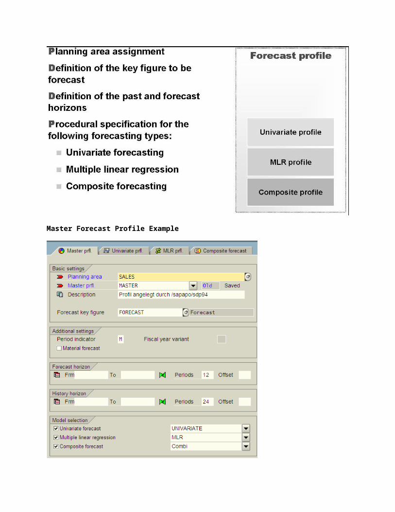
APO DP supports the following types of forecasting methods.

– Univariate (statistical)

– Multiple Linear Regression (MLR)

– Composite

Key Figure – A Definition

Key Figures are numeric or quantitative data that are useful for forecasting purposes.

APO DP has a built-in library containing many commonly used key figures. However, customer unique key figures may also be created.

Key figures usually appear as rows in spreadsheet looking screens.

Planning Areas

Planning Book/Data View Example

Creating The Selection ID

Drilling Down To Lower Details

Aggregating & Disaggregating

Aggregation is the automatic function by which key figure values on the lowest level of detail are summed at run time and displayed or planned on a high level

Disaggregation is the automatic function by which a key figure value on a high level is broken down to the detailed level.

Proportional Factors

Proportional factors are used to disaggregate the forecast.

They are derived from historical data and represent ratios or percentage.

For example, if a sales for product T-F200 in a certain time period was 1000.

T-F200 was sold from 3 locations:

– Location 1000 – sold 230 units

– Location 2400 - sold 450 units

– Location 2500 – sold 320 units

Therefore, the proportional factor for location 1000 is 230/1000 or 23%. That is, 23% of the sales for this time period occurred at location 1000.

Forecasting Pre-requisites

To generate a forecast in APO DP the following are hard pre-requisites:

– Master data in the form of characteristic-value-combinations (CVC)

– A selection ID – What to forecast

– A forecast profile – How to forecast?

Univariate Forecasting Techniques

Is a statistical forecast

Examples include:

– Moving average

– Constant models, trend models, seasonal models

– Exponential smoothing

– Seasonal linear regression

– The Holt-Winter.s method

– Croston.s method (for sporadic demand)

– Automatic selection

Master Forecast Profile

Master Forecast Profile Example

Multiple Linear Regression (MLR)

APO DP supports Multiple Linear Regression as a forecasting technique.

You use MLR to determine how a dependent variable, such as sales, is connected with independent variables called casual variables, such as prices, advertising, and seasonal factors.

MLR uses historical data as a basis to calculate the regression coefficients, b, for causal analysis.

The demand planner has the task to identify and quantify the most important independent variables and to model the causal connection

MLR Example

The Composite Forecast

Collaborative Forecasting

You collaborate with your customers over an internet connection.

Customers will view your statistical forecast and can give feedback on whether it is too high or too low.

The result can be improved forecast accuracy

Collaborative planning requires a strong business relationship between trading partners and most of TRUST.

Consensus Based Forecasting

APO DP supports consensus based forecasting.

Consensus based forecasting may be performed various ways including:

– Different planning books for different forecasting organizations

Consensus forecasting business meetings where all parties participate in arriving at the best possible forecast

The Alert Monitor

The APO Alert Monitor may be used to send alerts regarding important abnormal situations.

For Demand Planning the important abnormality is a forecast error that exceed a pre-defined threshold level.

For example,

– You wish to be alerted if a MAPE calculated forecast error exceeds 15%.

– If a given forecast has a MAPE of 22% an alert will be created.

Alerts may be delivered via several media including email.

Product Life Cycle (PLM)

Forecasting the demand for new products can be difficult since they have not previous historical data.

Additionally, forecasting the “end-of-life” for products being phased out is important from an inventory management point of view.

Product Life Cycle (PLM)

Product Life Cycle (PLM)

Promotion Planning

Promotions can be created to apply patterns to the demand forecast.

The patterns can be stored in the promotion pattern library and used, as required (multiple times).

The function is also available to detect promotion patterns in historical data and to create promotion patterns based on them

Promotion Planning

The Release Process

After the demand plan has been approved for it must be released for operations planning.

Various potential paths exist for releasing the demand plan. See the graphic on the next slide.

After the release process, the forecast requirements will be classified as planned independent requirements (PIR).

The forecast release almost always will contain four basic parameters: 1) product, 2) location, 3) quantity, and 4) time.

MRP in R/3 or SNP in APO may act on PIRs to create replenishment planned orders.

Forecast Data Flows

APO Release Architecture

DP Release Example

APO Release Architecture

Introduction To Supply Network Planning (SNP)

APO Supply Network Planning (SNP) is an intermediate time frame planning function.

Its primary purpose is to create a good rough-cut supply plan across the entire supply chain.

SNP may be used for either infinite or finite capacity planning.

Three separate and unique replenishment planning engines are bundled into SNP:

– Heuristic

– Capable-To-Match (CTM)

– Optimizer

In addition to supply and demand matching, SNP is capable of performing two additional supply chain management functions:

– Deployment

– Transportation Load Builder

APO Planning Horizons

SNP Process Flow

SNP Planning Engines

SNP Architecture

Order Based Live Cache

Interactive Supply Network Planning

The SNP Heuristic

The role of Heuristic planning to is to plan the supply to meet demand throughout the entire supply chain.

Heuristic planning is quantity-based planning. This means it will create a supply quantity for a specific time period regardless of the actual order quantities.

The SNP Heuristic plans in a level-by-level planning method similar to MRP in SAP R/3.

Heuristic planning assumes infinite capacity when planning.

Sourcing decisions (that is, what locations should be used as supplies) is driven primarily by Quota Arrangements.

Heuristic Example

The SNP Heuristic Scenario

Quota Arrangements In Heuristic

Other APO Master Data Used In Heuristic

SNP Capacity Balancing

SNP Heuristic planning is based on the assumption that resources have an infinite capacity.

After the SNP Heuristic run is complete, the planner can make a capacity check, which allows the planner to see the impact that planned orders will have on

resources and to quickly determine whether or not the plan is feasible.

If there is a capacity overload, an alert is displayed.

The planner can decide how to modify the production plan to meet demand before actually going into production.

Capacity Balancing Alternatives

Increase capacity through overtime or additional resources

Move work backward in time where capacity is available (subject to material availability)

Move work forward in time where capacity is availability (subject to material availability)

Move work to an alternate resource

Split the order (i.e. sub-divide) into quantities that will meet available capacity.

SNP Capacity Balance Example

SNP Capacity Leveling Example

Capacity Leveling Example

SNP Review

APO SNP is an intermediate range planning tool.

It will plan supplies to match demands using several potential software algorithms:

– Heuristic – infinite capacity planning only

– Optimizer – finite capacity planning

– Capable-To-Match (CTM) – infinite or finite capacity planning.

This lesson will focus on the use of the Optimizer and Capable-To-Match techniques

Linear Programming

Linear programming (LP) traces it history to the 1940’s as a method of solving complex planning problems with war time implications.

George Dantzig is considered the primary inventory of LP but John von Neumann is also considered by many as a co-inventor.

LP is a special class of mathematical problems in which a linear function (called the objective function) is either minimized (like costs) or maximized (like profits).

The other two components of a linear programming problem besides the objective function are:

– Decision variables

– Constraints

Linear Programming

Decision variables are used to model the various “decisions” that may be required in supply chain planning. Examples of decision variables are:

– What products should be produced?

– How much of each product should be produced?

– Where should the products be produced?

– How should the products be transported?

Constraints

– Constraints represent realities that essentially “bound” the solution options to that the result is feasible.

– Examples include:

• Demands must be met

• Cannot exceed capacity

• Storage capacity is limited

Non-Linear Programming

In many cases, the objective function may be non-linear. In this case other solution techniques must be employed. A few optimization techniques are:

– Non-linear programming (NLP)

– Mixed-Integer linear programming (MILP)

– Mixed integer non-linear programming (MINLP)

SAP APO supports LP and MILP problems.

APO SNP Optimizer

The Optimizer or “solver” in APO SNP uses linear programming to consider all relevant factors simultaneously.

SAP has embedded a 3rd party “solver” – ILOG CPLEX into the APO system.

The optimizer compares alternative solutions using costs that would be incurred. It determines the most cost-effective solution based on the constraints and objective function defined in the system.

You use penalty costs to prioritize demands. If a product brings high sales revenues, you set high penalty costs.

The result of the optimization run might be that due dates are violated or that safety stocks are not replenished

Optimizer

Capable To Match (CTM)

CTM is an order-based planning method, which means that every single sales order or Planned Independent Requirement PIR is planned separately.

CTM uses demand priorities as the primary basis performing supply network planning.

Demand priorities may be defined using multiple methods consistent with corporate policy or culture.

For example, demand priorities may be defined as:

– Preferred customer

– Due date

– Revenue

CTM is capable of panning with either finite or infinite capacity assumption.

CTM does not perform optimization. It terminates when it find the 1st feasible solution to the problem.

CTM Process

CTM Scenario

First Feasible Solution Example

Prioritizing Demands In CTM

Prioritizing Supplies In CTM

Safety Stock Planning

The following uncertainties occur during planning:

– Demand uncertainty (forecast)

– Replenishment lead time

To safeguard against these uncertainties, you can plan safety stock (SStk) as follows:

– Maintaining the safety stock manually in the product master

– Calculate the time-dependent safety stock in an SNP key figure in the Interactive Planning Table.

– Create a model dependent safety stock to achieve a certain customer service level.

APO SNP provides more sophisticated safety stock planning than R/3.

Model-Dependent Safety Stock

Deployment

At the time of actually executing the distribution plan, the stock levels, stock receipts and sales orders are not at the same levels as when the planning run was run last.

For example, SNP created a planned order for 500 during a planning run 3 months ago. The order due date is next week. However, there were production problems and the order qty is now 450.

This means that we can only distribute (that is, deploy) 450 instead of the 500 originally expected.

The SNP Deployment process will determine how the remaining 450 will be deployed to their respective destinations. It uses various “fair-share” rules.

Actual deployment orders are created in R/3

Deployment Fair Share Example

Transportation Load Builder (TLB)

Once the question of deployment has been determined, then we can begin to do some transportation planning.

Transportation Load Builder is a lite-transportation load builder that will optimize the use of the transportation fleet of vehicles.

TLB only creates full loads

TLB does not perform any route planning.

Actual transportation orders are created in R/3.

Transportation Load Builder (TLB)

Executing The Supply Plan

Supply Chain Engineer

The APO Supply Chain Engineer (SCE) is a convenient graphical tool that allows customers to graphically view and edit their APO master data objects.

With literally thousands of master data elements in a supply chain the management of master date can be become overwhelming.

The SCE allows a customer to create a filter containing those master data objects that are under his responsibility.

The resulting filtered master data objects is called a “work area”.

Model/Version

Supply Chain Engineer

SC Engineer

Defining Work Areas

Sample Supply Chain Engineer

The Risks Of Software Implementations

Software implementations can be a high risk, high cost and potentially disastrous process for a company.

Rarely are software implementations a slam dunk success!

Many factors influence the overall success of a software implementation including:

– Project manager

– Top management support

– Technical issue

– End user issues

– End user training

Software implementation methodologies reduce the risk and cost of a software implementation.

Software Implementation Methodologies

A methodology is a structured, proven process of accomplishing a task.

Software implementation methodologies have existed for many years. They are usually defined by major phases.

The SAP software implementation methodology consists of the following phases:

– Project preparation

– Business blueprint

– Realization

– Final preparation

– Go live & support

Project Preparation

The project preparation phase will define the general conditions for implementing the project successfully. It will include:

– Defining the goals and objectives of the project.

– Establishing the project organization

– Creating the project plan

– Determining the project standard procedures

– Training the project team

– Setting up the SAP 3-system landscape

– Creating a communication plan for the project

– Take certain benchmark measurements

Business Blueprint

The business blueprint phase is a critical phase in the methodology. Failure to take adequate time to lack of forward thinking in this phase will significantly increase the risk of the overall project.

Each major department being affected by the scope of the software will undertake an analysis of their current processes.

The resulting analysis will document the functional requirements that the new software implementation.

– Example – the SAP system should capable of automatically determining a source of supply for a requirement.

Realization

This phase will begin the implementation of the functional requirements defined in the Business Blueprint phase. This phase will include the following activities:

– Configuring the SAP system

– Setting up the test environment

– Setting up the security/administration settings

– Setting up any workflow processes

– Writing test scripts

Final Preparation

This phase will include the following activities:

– Loading master data

– Unit, function and integration testing

– End user training

– Customer sign-off

Go Live & Support

This phase will launch the new application and provide the necessary support for a period of time required to achieve institutionalization.

Activities include:

– End user re-training

– Software trouble call support

– Software de-bug support

– Configuration re-setting