Washington University in St. LouisWashington University Open Scholarship

Arts & Sciences Electronic Theses and Dissertations Arts & Sciences

Spring 5-15-2018

Advanced Methods in Comparative Politics:Modeling Without Conditional IndependenceDavid George CarlsonWashington University in St. Louis

Follow this and additional works at: https://openscholarship.wustl.edu/art_sci_etds

Part of the Political Science Commons

This Dissertation is brought to you for free and open access by the Arts & Sciences at Washington University Open Scholarship. It has been acceptedfor inclusion in Arts & Sciences Electronic Theses and Dissertations by an authorized administrator of Washington University Open Scholarship. Formore information, please contact digital@wumail.wustl.edu.

Recommended CitationCarlson, David George, "Advanced Methods in Comparative Politics: Modeling Without Conditional Independence" (2018). Arts &Sciences Electronic Theses and Dissertations. 1517.https://openscholarship.wustl.edu/art_sci_etds/1517

WASHINGTON UNIVERSITY IN ST. LOUIS

Department of Political Science

Dissertation Examination Committee:

Jacob M. Montgomery, Chair

Roman Garnett

Jeff Gill

Guillermo Rosas

Margit Tavits

Advanced Methods in Comparative Politics:

Modeling Without Conditional Independence

by

David George Carlson

A dissertation presented to

The Graduate School

of Washington University in

partial fulfillment of the

requirements for the degree

of Doctor of Philosophy

May 2018

St. Louis, Missouri

c©2018, David George Carlson

Table of Contents

List of Figures v

List of Tables vi

Acknowledgements vii

Abstract ix

Introduction 11.1 Modeling Related Processes with an Excess of Zeros . . . . . . . . . . . . . . 21.2 Modeling Without Conditional Independence: Gaussian Process Regression

for Time-Series Cross-Sectional Analyses . . . . . . . . . . . . . . . . . . . . 51.3 Executive Moderation and Public Approval in Latin America . . . . . . . . . 61.4 Concluding Remarks . . . . . . . . . . . . . . . . . . . . . . . . . . . . . . . 7

Modeling Related Processes with an Excess of Zeros 102.5 Zero-Inflated and Correlated Errors: Issues and Solutions . . . . . . . . . . . 13

2.5.1 Models with Zero-Inflation and Seemingly Unrelated Regressions . . . 132.5.2 Partial observability in strategic settings . . . . . . . . . . . . . . . . 14

2.6 ZIMVOP Specification . . . . . . . . . . . . . . . . . . . . . . . . . . . . . . 152.6.1 First Step . . . . . . . . . . . . . . . . . . . . . . . . . . . . . . . . . 162.6.2 Second Step . . . . . . . . . . . . . . . . . . . . . . . . . . . . . . . . 172.6.3 Likelihood . . . . . . . . . . . . . . . . . . . . . . . . . . . . . . . . . 182.6.4 Priors . . . . . . . . . . . . . . . . . . . . . . . . . . . . . . . . . . . 19

2.7 Applying ZIMVOP . . . . . . . . . . . . . . . . . . . . . . . . . . . . . . . . 202.7.1 Implementation on Simulated Data . . . . . . . . . . . . . . . . . . . 202.7.2 Application: Presidential Campaigns in Mexico . . . . . . . . . . . . 26

2.8 Conclusion . . . . . . . . . . . . . . . . . . . . . . . . . . . . . . . . . . . . . 30

Modeling Without Conditional Independence: Gaussian Process Regressionfor Time-Series Cross-Sectional Analyses 323.9 Time-Series Cross-Sectional Analyses: Issues and Solutions . . . . . . . . . . 34

3.9.1 Prevalence of Current Approaches . . . . . . . . . . . . . . . . . . . . 363.9.2 Fixed-Effects Specifications . . . . . . . . . . . . . . . . . . . . . . . 36

ii

3.9.3 Random-Effects Specifications . . . . . . . . . . . . . . . . . . . . . . 393.9.4 Clustering Standard Errors . . . . . . . . . . . . . . . . . . . . . . . . 393.9.5 Correcting for Serial Correlation . . . . . . . . . . . . . . . . . . . . . 41

3.10 Gaussian Process Regression for TSCS Data . . . . . . . . . . . . . . . . . . 413.10.1 GPR Specification . . . . . . . . . . . . . . . . . . . . . . . . . . . . 433.10.2 Priors . . . . . . . . . . . . . . . . . . . . . . . . . . . . . . . . . . . 47

3.11 Applying GPR . . . . . . . . . . . . . . . . . . . . . . . . . . . . . . . . . . 483.11.1 Implementation on Simulated Data . . . . . . . . . . . . . . . . . . . 493.11.2 Application: The Effect of Inflation on Anti-Americanism in Latin

America . . . . . . . . . . . . . . . . . . . . . . . . . . . . . . . . . . 583.11.3 Replication: The Effect of the Threat of Rockets on the Right-Wing

Vote in Israel . . . . . . . . . . . . . . . . . . . . . . . . . . . . . . . 643.12 Conclusion . . . . . . . . . . . . . . . . . . . . . . . . . . . . . . . . . . . . . 65

Executive Moderation and Public Approval in Latin America 684.13 Theoretical Expectations . . . . . . . . . . . . . . . . . . . . . . . . . . . . . 704.14 Data and Method . . . . . . . . . . . . . . . . . . . . . . . . . . . . . . . . . 76

4.14.1 Variables . . . . . . . . . . . . . . . . . . . . . . . . . . . . . . . . . . 774.14.2 Modeling Choice: Gaussian Process Regression . . . . . . . . . . . . 82

4.15 Results . . . . . . . . . . . . . . . . . . . . . . . . . . . . . . . . . . . . . . . 844.15.1 Comparison to Alternative Modeling Choices . . . . . . . . . . . . . . 91

4.16 Conclusion . . . . . . . . . . . . . . . . . . . . . . . . . . . . . . . . . . . . . 96

Concluding Remarks 985.17 Related Future Work . . . . . . . . . . . . . . . . . . . . . . . . . . . . . . . 100

References 103

Appendix 1157.18 Modeling Related Processes with an Excess of Zeros Supplementary Information115

7.18.1 ZIMVOP JAGS Model . . . . . . . . . . . . . . . . . . . . . . . . . . 1157.18.2 ZIMVOP Simulation Exercise . . . . . . . . . . . . . . . . . . . . . . 1177.18.3 Presidential Campaigns in Mexico . . . . . . . . . . . . . . . . . . . . 120

7.19 Executive Moderation and Public Approval in Latin America SupplementaryInformation . . . . . . . . . . . . . . . . . . . . . . . . . . . . . . . . . . . . 122

iii

List of Figures

2.1 Parties’ decision trees. . . . . . . . . . . . . . . . . . . . . . . . . . . . . . . 122.2 Results of the simulations varying the degree of zero-inflation. . . . . . . . . 232.3 Results of the simulations varying correlations. . . . . . . . . . . . . . . . . . 252.4 Results from the presidential campaign visits in Mexico. . . . . . . . . . . . 29

3.5 Inflation and anti-Americanism in Mexico . . . . . . . . . . . . . . . . . . . 353.6 Two-way fixed-effects model fit and residuals of inflation in Latin American

countries over time . . . . . . . . . . . . . . . . . . . . . . . . . . . . . . . . 383.7 GPR fit of inflation in Latin American countries over time . . . . . . . . . . 443.8 Example simulated serial correlation data, ρ = 0.9 . . . . . . . . . . . . . . . 513.9 Results of simulations with varying degrees of serial correlation in error and

explanatory variable . . . . . . . . . . . . . . . . . . . . . . . . . . . . . . . 523.10 Results of simulations with varying degrees of correlation between group in-

tercept and explanatory variable . . . . . . . . . . . . . . . . . . . . . . . . . 543.11 False positive rates across models . . . . . . . . . . . . . . . . . . . . . . . . 553.12 Results of simulations with varying number of units and observations per unit 573.13 Estimated effect of inflation on anti-Americanism . . . . . . . . . . . . . . . 613.14 Actual data points and posteriors in Mexico . . . . . . . . . . . . . . . . . . 623.15 Estimated effect of being within bomb range on right vote . . . . . . . . . . 66

4.16 Theoretical expectations for the effect of moderation conditional on extremity 734.17 Histogram of Approval difference . . . . . . . . . . . . . . . . . . . . . . . . 784.18 Histogram of Ideological moderation . . . . . . . . . . . . . . . . . . . . . . . 794.19 Histogram of Extremity . . . . . . . . . . . . . . . . . . . . . . . . . . . . . . 804.20 The effect of moderation on changes in approval . . . . . . . . . . . . . . . . 844.21 The effect of moderation on changes in approval conditional on extremity . . 864.22 The predicted point-wise effect of moderation on changes in approval as ex-

tremity increases . . . . . . . . . . . . . . . . . . . . . . . . . . . . . . . . . 874.23 The effect of election year on executive moderation . . . . . . . . . . . . . . 884.24 The effect of election year on executive moderation conditional on extremity 904.25 The predicted point-wise effect of election year in election years on moderation

as extremity increases . . . . . . . . . . . . . . . . . . . . . . . . . . . . . . . 91

iv

4.26 The predicted point-wise effect of election year in non-election years on mod-eration as extremity increases . . . . . . . . . . . . . . . . . . . . . . . . . . 92

4.27 The effect of executive moderation on changes in public approval, model com-parison . . . . . . . . . . . . . . . . . . . . . . . . . . . . . . . . . . . . . . . 93

4.28 The effect of executive moderation on changes in public approval conditionalon extremity, model comparison . . . . . . . . . . . . . . . . . . . . . . . . . 94

4.29 The effect of election year on executive moderation, model comparison . . . 954.30 The effect of election year on executive moderation conditional on extremity,

model comparison . . . . . . . . . . . . . . . . . . . . . . . . . . . . . . . . . 96

7.31 Comparing ZIMVOP to a model without correlations on the main application 121

v

List of Tables

4.1 Theoretical expectations for the effect of movement . . . . . . . . . . . . . . 714.2 Theoretical expectations for movement . . . . . . . . . . . . . . . . . . . . . 71

7.3 True parameters for the first round of simulations . . . . . . . . . . . . . . . 1187.4 True parameters for the second round of simulations . . . . . . . . . . . . . . 1197.5 Posterior β estimates for the first hypothesis . . . . . . . . . . . . . . . . . . 1227.6 Posterior β estimates for the second hypothesis . . . . . . . . . . . . . . . . 1227.7 Posterior β estimates for the third hypothesis . . . . . . . . . . . . . . . . . 1227.8 Posterior β estimates for the fourth hypothesis . . . . . . . . . . . . . . . . . 123

vi

Acknowledgements

I would like to sincerely thank Jacob M. Montgomery, my chair, for his countless hours of

work providing invaluable feedback and support. I would also like to thank my committee,

Roman Garnett, Jeff Gill, Guillermo Rosas, and Margit Tavits, for their time and effort.

The Washington University Political Data Science Lab deserves immense recognition for

comments on many early drafts of this dissertation. Finally, the members of the Comparative

Politics Workshop at Washington University provided incredibly useful critiques throughout

this project’s development.

David George Carlson

Washington University

May 2018

vii

Dedicated to Elif Ozdemir

viii

ABSTRACT OF THE DISSERTATION

Advanced Methods in Comparative Politics:

Modeling Without Conditional Independence

by

David George Carlson

Doctor of Philosophy in Political Science

Washington University in St. Louis, 2018

Professor Jacob M. Montgomery, Chair

One of the most significant assumptions we invoke when making quantitative inferences is the

conditional independence between observations. There are, however, many situations when

we may doubt this independence. For instance, two seemingly distinct data-generating pro-

cesses may in fact share unobserved relations. Time-series and cross-sectional studies are also

plagued by a lack of independence. If we ignore this common violation of our fundamental

modeling assumptions we may draw improper conclusions from our data. This dissertation

introduces two methods to the political science literature: a zero-inflated multivariate or-

dered probit and Gaussian process regression for time-series cross-sectional analyses. This

latter model is then applied to demonstrate that executives in Latin America enjoy increased

public support following ideological moderation, but executives are less willing to moderate

during election years. These effects, however, are conditional on the extremity of the execu-

tive. The dissertation as a whole contributes both methodologically and theoretically to the

field.

ix

Introduction

When making quantitative inferences in political science, one of the most significant assump-

tions we invoke is the conditional independence between observations. There are, however,

many situations when we may doubt this independence. For instance, two seemingly distinct

data-generating processes may in fact share unobserved relations (Zellner 1962; Zellner and

Huang 1962). Time-series and cross-sectional studies are also plagued by a lack of inde-

pendence (Pang 2014). If we ignore this common violation of our fundamental modeling

assumptions we may draw improper conclusions from our data.

Although political science has made great strides to better recognize and address these

issues (e.g., Monogan 2015, Ch. 9), the best practices for the analyses of certain types of data

remain elusive. For example, time-series cross-sectional analyses have become increasingly

sophisticated, yet there is no default solution, and for any given problem the “best” solution

is often still not ideal. Similarly, multivariate analyses for related processes are under-utilized

and have not been expanded in scope to some of the more advanced and newly developed

models.

In this dissertation, I present three chapters to fill these gaps. The first, “Modeling Re-

lated Processes with an Excess of Zeros,” extends existing models and develops a zero-inflated

multivariate ordered probit model. Political science research frequently models binary or or-

dered outcomes involving related processes. However, traditional modeling of these outcomes

ignores common data issues and cannot capture nuances. There is often an excess of zeros,

1

the observed outcomes for different actors are inherently related, and competing actors may

respond to the same factors differently. The proposed model is ideal for capturing strategic

interactions between competing parties when there exist resource constraints. The model

allows and estimates correlations between the competing actors’ decision processes. Not

only does it relax our assumptions that these outcomes are independent, but it provides the

means to measure the degree of interaction. I apply the model to presidential campaign

strategies in Mexico.

The next chapter, “Modeling Without Conditional Independence: Gaussian Process Re-

gression for Time-Series Cross-Sectional Analyses,” utilizes a machine-learning approach to

regression and develops a novel technique to model time-series cross-sectional data. Simu-

lations show that it out-performs extant models commonly used for these types of data. I

apply this model to better understand the effect of inflation on anti-Americanism in Latin

America, and I replicate an analysis on the effect of rocket threat on the right-wing vote in

Israel.

The next chapter, “Executive Moderation and Executive Approval in Latin America,” is

a more detailed application of the Gaussian process to show the relationship between Latin

American executives’ use of position-taking in annual addresses and public approval. This is

an ideal application for the Gaussian process regression model and an important substantive

question. I will now outline the three chapters in more detail.

1.1 Modeling Related Processes with an Excess of Ze-

ros

Political scientists frequently test hypotheses in which the outcome variable is binary or or-

dered. However, there are often two distinct challenges analyses of this sort encounter. The

outcome variable exhibits an excess of zeros, and the data-generating process for multiple

2

outcomes may be related. This is particularly true when studying strategic interactions be-

tween political actors who must allocate scarce resources. As an example, consider campaign

decisions by competing parties to visit municipalities. Campaigns can only realistically visit

a small proportion of these municipalities, so the outcome, a visit, exhibits an excess of zeros.

Further, there are likely decisions made based on covariates to never even consider visiting

certain municipalities. To add to the complication of the true data-generating process, the

decisions made by the parties to visit are likely highly interdependent. Parties are very likely

responding to the anticipated or observed behavior of their competitors.

Ignoring either of these issues – zero inflation and strategic interdependence – can bias

parameter estimates, and typical modeling strategies tend to have inefficient estimators. Fur-

thermore, by failing to address these problems, we miss an opportunity to better understand

important nuances of the underlying dynamics of the data generating process. Returning to

the example of campaign visits, we should be interested in the factors that lead to a munic-

ipality being considered for a visit, even if the party never actually visits (the outcome is a

zero). There are thus two types of observed zeros, and we wish to be able to discriminate

between them to better understand the parties’ calculi. We also want to test the proposition

that these decisions are in fact related, and the parties are strategically interacting.1 Finally,

different actors may have different decision-making criteria. For example, parties may not

respond to covariates in the same way. We want to be able to test for this heterogeneity and

explore the various relationships of our variables of interest.

In this chapter, I extend the zero-inflated ordered probit (Harris and Zhao 2007) to better

address these issues by allowing for interdependent multivariate outcomes, developing a zero-

inflated multivariate ordered probit (ZIMVOP). This model is novel not only to political

science, it has yet to be developed in any literature. It consists of two steps. The first

1Because these decisions are being made at an unobserved time, or simultaneously, standard strategicinteraction models are inappropriate (Bas, Signorino, and Walker 2008; Carson and Roberts 2005; Signorino2002; Signorino 2003).

3

step models the observation as a potential non-zero, splitting the population into “always

zeros” and “potential non-zeros.” The second step is a multivariate ordered probit, allowing

correlations of the disturbance terms across equations over dimensions.

To make this model more concrete, and to provide a running example, I re-analyze a

dataset of Mexican presidential campaign visits in 2006 and 2012 for the three major parties

– the Partido Revolucionario Institucional (PRI), the Partido Accion Nacional (PAN), and

the Partido de la Revolucion Democratica (PRD) (Langston and Rosas 2016). The outcome

of interest is the level of visitation by each of the parties – no visit, hold a meeting, or hold

a rally. Because there are three parties, the outcome is trivariate. In other words, each

municipality has three outcomes, one for each party, that are inherently related. Further,

the vast majority of the municipalities were never visited by any party.

Extant models cannot capture the nuances I have described. Zero-inflated models would

not test for or allow the heterogeneity if the data are pooled. If separate zero-inflated models

are run for each party, we could not test if there exists strategic interdependence in their

visit strategies. Models allowing correlations between outcomes (e.g., seemingly unrelated

regressions) would not capture the zero inflation. I show through simulation exercises that

ZIMVOP also outperforms the extant alternatives by reducing bias and increasing efficiency.

Therefore, if ZIMVOP were not employed on data suffering these two issues, besides not

capturing nuances, we may come to incorrect substantive conclusions. The contribution of

this chapter, therefore, is to provide a model that can correctly account for both zero inflation

and strategic interactions to allow political science researchers to better understand these

kinds of processes.

4

1.2 Modeling Without Conditional Independence: Gaus-

sian Process Regression for Time-Series Cross-Sectional

Analyses

Researchers in political science very frequently need to analyze panel data or time-series

cross-sectional data. There are well-known problems these analyses encounter, however,

such as time-varying confounders, serial correlation in the variables of interest across time,

between-subject heterogeneity, spatial correlations, and more, that make inferences partic-

ularly difficult. Both parameter estimates and their standard errors can be misleading and

biased when inappropriately modeled, often leading to spurious results (Granger and New-

bold 1974). Esarey and Menger (2017) provide a thorough analysis of the more common

solutions to these problems, including hierarchical modeling and various ways of adjusting

standard errors. Although the article offers good suggestions for various situations, there is

no default solution and the best option for a given data set can still produce excessive false

positives and negatives, biased estimates, and tend to be inefficient. This chapter offers a

different modeling strategy utilizing Gaussian process regression (GPR) that surpasses ex-

tant alternatives on many criteria across a range of situations, and may serve as a better

default option for applied research than any used in current practice. It offers the simplicity

of standard inferential techniques while handling complex underlying data-generation.

GPR is primarily known for its uses in machine learning classification and prediction

(Rasmussen and Williams 2006), but the models have been utilized to make inferences about

populations as well (e.g., Kirk and Stumpf 2009; Huang, Zhang, and Scholkopf 2015; Garg,

Singh, and Ramos 2012; Qian, Zhou, and Rudin 2011; Gibson et al. 2012). Monogan and Gill

(2016) use a GPR approach, which they refer to as Bayesian kriging, to estimate a posterior

density blanket of citizens’ ideologies across the United States. Despite having relatively

5

sparse data, the method allows for any level of geographic aggregation and provides an

estimate, with uncertainty, of the ideology of the region by smoothing across space.

This smooth blanket over the U.S. is a useful introduction to conceptualize GPR. Data,

in this case, some measure capturing ideology, is not independent. The average ideology

in a town is likely similar to the ideology in its neighboring towns. We can consider these

outcomes (ideology) as coming from a joint normal distribution if we assume each realization

comes from a normal distribution. A Gaussian process is a distribution over function space,

with each observed outcome coming from a normal distribution, making the joint distribution

a multivariate normal. We do not need to consider data as independent, and we do not need

to impose many assumptions on the relationship of the correlational structure.

The “smoothing” across space is intuitive, but we can smooth over any input dimension

we choose, including, of course, time. The same way neighboring towns are likely heavily

correlated, so too are temporally proximate observations, or observations sharing similar

explanatory variables. These correlations can also vary from dimension to dimension. In

other words, temporally proximate observations need not share the same correlation as ge-

ographically proximate observations. Rather than considering data as independent, or even

sequential, we can think of all observations as coming from one joint distribution, with data

points close to each other in the hyperplane likely similar. The flexibility of the model makes

it ideal for modeling situations in which there are violations of the conditional independence

assumption but the nature of these correlations is not known a priori.

1.3 Executive Moderation and Public Approval in Latin

America

It is very common for executives in Latin America to shift their professed ideology or policy

positions over the course of their tenure as president (Arnold, Doyle, and Wiesehomeier

6

2017). However, the literature on the region has not fully investigated the effect this has on

executive public approval, and as such is missing a critical explanation for this movement. I

argue that moderation, i.e., moving closer to the median voter, boosts public approval overall.

Further, these benefits are enjoyed most by extreme executives, whose movement is more

noticeable and whose moderation increases the utility of voters more than moderation by

centrist executives. This gives an added incentive for presidents to moderate their professed

ideology, because public approval increases their legislative bargaining power (Calvo 2007).

There are costs associated with this movement, however. Executives, particularly extreme

executives, rely on relatively extreme supporters who turn out to vote and are more politically

active (Samuels and Shugart 2010; Samuels 2008b). Because of this, presidents have an

incentive to shift their professed ideology towards the extremes during either executive or

legislative election years. This helps turn out their voters and activists to ensure personal

and / or party electoral success.

To test these claims, I rely on ideal points estimated from the constitutionally mandated

annual addresses of presidents (Arnold, Doyle, and Wiesehomeier 2017) to capture their

professed positions on a left-right scale over time. I also utilize time-series public approval

data estimated from representative surveys (Carlin et al. 2016). Standard analyses of these

data are problematic for all of the reasons discussed in the previous chapter, making Gaus-

sian process regression a proper strategy. The models support my hypotheses. Alternative

modeling strategies provide mixed results, but in general are largely consonant with GPR.

1.4 Concluding Remarks

The following three chapters all highlight the issues with ignoring violations to the commonly

invoked assumption of conditional independence. Traditional modeling in political science

can lead to biased estimates, tend to be inefficient, and, perhaps the worst drawback, may

7

lead to incorrect substantive conclusions. There is very frequently reason to doubt con-

ditional independence when analyzing social science data, yet, as the chapters will argue,

ignoring the violation is unfortunately quite common in the discipline.

Besides discussing the issues associated with this problem and arguing for more careful

modeling, I also propose novel solutions to model some of the more common types of data

encountered in political science, particularly comparative political science. The first model,

a zero-inflated multivariate ordered probit, has never been developed in any literature. The

second model, Gaussian process regression for time-series cross-sectional (TSCS) analyses, is

a unique parameterization of an under-utilized statistical model specifically for TSCS data.

I thus am both introducing the model to political science and demonstrating how it can be

modified to fit our purposes as social scientists.

The dissertation also adds to our theoretical understanding of core political concepts.

The first of the three chapters demonstrates that parties in Mexico in competition with one

another while campaigning have varying motivations and strategies to visit or hold rallies in

particular municipalities. Further, the chapter demonstrates that these decisions are related

to one another. This is both an interesting substantive finding and justifies the use of a

model that does not assume conditional independence.

The second of the three chapters demonstrates that across Latin America inflation leads

to less anti-Americanism in the region. Latin American citizens view the United States

as a source of economic well-being. When they feel the pressure of declining purchasing

power they want their countries to increase relations with the United States to improve

their economic situation. Standard approaches to modeling these data fail to uncover this

interesting finding.

Finally, the third chapter explores in depth the effects of Latin American executive ide-

ological moderation on public approval, shedding light on the motivations presidents in the

region have for dampening their policy or ideological stances. While executives, especially

8

extreme executives, benefit from moderation, they do so at the cost of disappointing party

activists and extreme voters who turn out. Executives are therefore less willing to moderate

during electoral years to benefit themselves and / or their party electorally.

This dissertation therefore examines a methodological issue in the discipline, begins to

address and solve some of these issues, and contributes to our understanding of Latin Amer-

ican politics and politics more generally. Following the three chapters I have discussed thus

far, I conclude with a discussion of the contribution and directions for future work. There is

also a short appendix for the second and fourth chapters.

9

Modeling Related Processes with an

Excess of Zeros

In many settings, political scientists wish to test theories where they must confront two dis-

tinct data challenges: (1) there is often an excess of zeros in the outcome variable, and (2) the

data generating process for multiple outcomes may be related. This is particularly true when

studying related decisions between political actors who must allocate scarce resources. For

instance, consider the decision-making processes of competing parties regarding candidate

visits during a presidential campaign. In practice, these campaigns can only visit a small

proportion of localities within a country during a single campaign. (The outcome exhibits

an excess of zeros.) Thus, many municipalities are never considered worthwhile for visits by

any candidate due their small populations or non-competitive nature. To make things more

complicated, however, of those municipalities that are worthwhile to (potentially) visit, deci-

sions by campaigns are also interdependent. That is, parties may visit municipalities simply

because they anticipate that they will be visited by their opponents, or actors may make

decisions based on similar but unobserved factors.

Ignoring either of these issues – zero inflation and interdependence – can bias parameter

estimates and decrease the efficiency of the estimators. Furthermore, by failing to address

them, we miss an opportunity to better understand important features of the data generating

process. What factors are related to being either a unit that is considered for resource

10

allocation or excluded completely? Is there really evidence that the behavior of one actor

is related to, or even shaped by, the (anticipated) behavior of other actors?2 Finally, do

different actors respond heterogeneously to different factors?

In this chapter, I extend the zero-inflated ordered probit (Harris and Zhao 2007) to

better address these issues by allowing for interdependent multivariate outcomes, developing

a zero-inflated multivariate ordered probit (ZIMVOP). It consists of two steps. The first

step models the observation as a potential non-zero, splitting the population into “always

zeros” and “potential non-zeros.” The second step is a multivariate ordered probit, allowing

correlations of the disturbance terms across equations over dimensions.

To make this model more concrete, and to provide a running example, I re-analyze a

dataset of Mexican presidential campaign visits in 2006 and 2012 for the three major parties

– the Partido Revolucionario Institucional (PRI), the Partido Accion Nacional (PAN), and

the Partido de la Revolucion Democratica (PRD) (Langston and Rosas 2016). The outcome

of interest is the level of visitation by each of the parties – no visit, hold a meeting, or hold

a rally. Because there are three parties, the outcome is trivariate. In other words, each

municipality has three outcomes, one for each party, that are inherently related. Further,

the vast majority of the municipalities were never visited by any party. Figure 2.1 provides

a graphical depiction of the parties’ decisions.

Unfortunately, no current model can accurately capture the decision tree described. Zero-

inflated models cannot measure the extent of interdependence between parties’ decisions.

Models allowing correlations between outcomes (e.g., seemingly unrelated regressions) would

not capture the zero inflation. Both approaches are inefficient and could lead to inaccurate

estimates and potentially incorrect conclusions. The contribution of this chapter, therefore,

2Because these decisions are being made at an unobserved time, or simultaneously, standard strategicinteraction models are inappropriate (Bas, Signorino, and Walker 2008; Carson and Roberts 2005; Sig-norino 2002; Signorino 2003). Further, the interdependence can arise from unobservables as well as strategicinteractions.

11

Figure 2.1: Parties’ decision trees.

not visitable visitable

Municipality

don’t go

PRI PAN PRD

don

’tgo

meetin

g

rally

don

’tgo

meetin

g

rally

don

’tgo

meetin

g

rally

Note: The decision of a party is split into two steps. The first decision is whether or nota municipality is visitable. The second decision is the type of visit, conditional on themunicipality being visitable. This decision is likely related to the decisions of other parties.

is to provide a model that can correctly account for both zero inflation and interdependence

to allow political science researchers to better understand these kinds of processes.

The outline of the chapter is as follows. First, I discuss the issues of zero-inflated and

correlated outcomes, and explain how ZIMVOP addresses both. As part of the discussion, I

discuss both its relationship to existing statistical approaches and also its distinct advantages.

Second, I provide the details for the ZIMVOP model. Third, I demonstrate its effectiveness

using simulated data and an application to the Mexican Elections example discussed above.

I conclude with a discussion of the limitations of the approach as well as potential future

applications.

12

2.5 Zero-Inflated and Correlated Errors: Issues and

Solutions

In this section, I discuss the issues associated with outcomes that exhibit an excess of zeros

and current approaches to dealing with these issues. I then do the same for multivariate

models that have correlated error terms, known as seemingly unrelated regressions (SUR).

Neither of these families of models adequately addresses the problems of both zero-inflated

outcomes and correlated error terms. Through the discussion, I highlight the advantages to

current approaches and demonstrate that ZIMVOP, a synthesis of the two families of models,

is an intuitive extension when dealing with data that raise both of these concerns.

2.5.1 Models with Zero-Inflation and Seemingly Unrelated Re-

gressions

King and Zeng (2001a and 2001b) introduce a unique approach to modeling rare outcomes,

focusing primarily on international conflict. They argue that modeling conflict on all country

dyads underestimates the effect of certain factors, producing biased estimates. This is due to

the fact that the vast majority of dyads will never go to war, regardless of certain observed

characteristics that may actually be deterministic in other dyads. The approach they suggest

is to save data collection, maintain all non-zero observations in the data, randomly sample

zero outcomes, and focus more time on the quality of the data than the quantity of data.

This recommendation saves data collection and may lead to less biased estimates relative

to running a standard probit on lower-quality data. However, observed zeros may have

distinct data-generating processes, suggesting a split-population approach (Harris and Zhao

2007). This split-population method differs from the rare events method by modeling the

outcome in two steps. The first step models the probability that an observation is a potential

13

non-zero, and the second step models the outcome conditional on the observation being a

potential non-zero. The split-population refers to splitting the population into “potential

non-zeros” and “always zeros.” An intuitive example relates to civil conflict. Bagozzi, Hill,

Moore, and Mukherjee (2015), using a zero-inflated ordered probit, find that a country’s

GDP has a reliable and negative effect on the potential for political violence, but on a

potential non-zero, the effect is positive. That is, rich countries are less likely to experience

political violence, but on a potential non-zero, income has a positive effect on the outcome,

likely due to greater resources.

This example highlights both the issues related to ignoring an excess of zeros and the

benefits in addressing them. If the two steps were ignored, the nuanced effects of these

covariates would be lost and the estimates of the effects would be biased, because a stan-

dard model with no inflation would lead to a correlation between the error terms and the

explanatory variables (Bagozzi and Marchetti 2014; Dunne and Tian n.d.).

In addition to the problems associated with an excess of zeros, outcomes also may share

related data-generating processes. The SUR class of models stacks regressions and allows

the error terms across these stacked regressions to be correlated (Zellner 1962). Jointly

estimating a set of equations improves asymptotic relative efficiency over the equation-by-

equation case by combining information across equations (King 1989; Zellner and Huang

1962). In other words, in the limit, the estimators produce estimates with smaller mean

squared errors and smaller variances.

2.5.2 Partial observability in strategic settings

The ZIMVOP model I propose below seeks to combine the approaches above in order to

achieve three simultaneous goals: (1) understand the relationship between the main explana-

tory variables and the outcome, (2) understand the process that leads some observations to

be excluded from consideration, and (3) detect inter-dependencies in the data generating

14

process for multiple outcomes. While several of the models above can achieve one or two of

these goals, none can accomplish all three simultaneously.

Nonetheless, it is important to note that there are several other models in the literature

that are similar in important ways to my own. Gurmu and Dagne (2012) developed a

zero-inflated bivariate ordered probit, but it does not easily extend to the multivariate case

(see also Kadel 2013).3 ZIMVOP generalizes this zero-inflated ordered probit to have a

theoretically unbounded number of dimensions in an intuitive, straight-forward manner.

Another project for settings with partially observable outcomes is presented by Nieman

(2015), who proposes a model for strategic interactions in a two-player, sequential game.

Similar to ZIMVOP, we observe the same outcome from two distinct data-generating pro-

cesses (status quo or government acquiesces). Despite the seeming similarity, the underlying

behavior modeled by ZIMVOP and Nieman are quite distinct, with the former estimating

related decision-making or processes, and the latter modeling a strategic game.

2.6 ZIMVOP Specification

ZIMVOP has two major components that in combination set the model apart from current

approaches. The first is a zero-inflation step. This is simply a univariate standard probit

that models the probability that an observation is a potential participator, or a potential

non-zero. In the Mexico example, this is whether or not any party will even consider visiting

a given municipality. This follows the zero-inflated ordered probit approach developed by

Harris and Zhao (2007).

The second component is a multivariate ordered probit for the final outcomes. For each

observation, there is a vector of outcomes, one scalar outcome for each dimension. In the

Mexico example, the “dimensions” are each party, one dimension for the PRI, one for the

3The principles of ZIMVOP do not vary substantially from these bivariate models, but the implementa-tion is much more straight-forward and these bivariate approaches only allow for one correlation parameter.

15

PAN, and one for the PRD. Each observation is a municipality in a given time period, and

the outcome is a vector of length three, with one outcome for each party. The outcome for

each component takes one of three values: 0 for no visit, 1 for a meeting, and 2 for a rally.

In this step, conditional on being a potential non-zero (e.g., a visitable municipality), an

ordered outcome is modeled separately for each dimension, but the error terms are allowed

to correlate across dimensions (parties). In other words, the decision processes at the second

step for each party are not assumed independent in a given municipality and time period.

In presenting the model, I follow the presentations of Harris and Zhao (2007), Gurmu and

Dagne (2012), and Kadel (2013). This setup requires that we model the observed outcome

for unit i on dimension r, yri, as the product of two unobserved discrete latent parameters,

yri = sizri, where si indicates whether unit i is a potential non-zero, and zri is the estimated

level of outcome conditional on observation i being a potential non-zero. In our Mexico

example, si ∈ 0, 1 represents whether a municipality is “visitable” by one of the parties,

while zri ∈ 0, 1, 2 is the model’s estimate of whether there will be no visit (0), a meeting

(1), or a rally (2) by party r in that municipality.

2.6.1 First Step

Both the first-step probit and the second-step multivariate ordered probit follow Albert

and Chib’s (1993) data augmentation approach such that we include in our model latent

parameters. Sampling of latent parameters leads to probability distributions for the observed

outcomes, and significantly improves computational tractability.

Let s∗i be a latent parameter capturing the potential for observation i to be a non-zero

(visitable) observation such that the probability of i being a non-zero is equal to Pr(s∗i > 0).

This latent value is modeled as a linear function of a matrix of covariates, V, with each row,

vi, being a vector of observation-level covariates (including a constant). Specifically, we let

s∗i = v′iγ + µi, where γ is a vector of unknown parameters to be estimated and µi is the

16

error term such that µi ∼ N(0, 1).4

Now, let si, the latent categorical parameter indicating potential non-zero observations,

be defined as:

si =

0 if s∗i ≤ 0,

1 if s∗i > 0.

Let Φ(·) denote the normal cumulative distribution function. Then,

Pr(si = 1) = Φ(s∗i ) = Φ(v′iγ)

is the probability of the observation being a potential non-zero.

2.6.2 Second Step

In the second step, let r = 1, . . . , D, where D is the total number of dimensions. The

Mexico example has a trivariate outcome (D = 3), with r equal to 1, 2, and 3, each number

indicating a party. Again following the standard data augmentation approach, let z∗ri be the

latent parameter related to the outcome level for observation i on dimension r conditional

on observation i being a potential non-zero. These levels of participation for the Mexico

parties are, in order: do not go (0), go for a meeting (1), or go for a rally (2). Let Xr be

a n by p matrix of predictors for the level of participation on dimension r (which includes

a constant). Let the n by p by D array of all second-step predictors for all dimensions be

denoted X . We let z∗ri = x′riβr+εri, where εri is the error term and βr is the unknown vector

to be estimated for dimension r.

Our goal is to estimate the latent categorical parameter zri, which is the level of participa-

tion for observation i on dimension r conditional on being a potential non-zero. In the data

augmentation approach, to allow for multiple categories, we need to also estimate a vector

of “cutoff” parameters (Albert and Chibb 1993). Let ar be the vector of cut-off points of

4The standard normal distribution is used to identify the model, although other choices could be used.I discuss all the prior distributions in Section 3.3.

17

length jr, where jr is the maximum possible outcome on dimension r (in our example jr = 2

for all r), and ark is the kth cutoff on dimension r. We can now define zri as:

zri =

0 if z∗ri ≤ ar1,

k if ark < z∗ri ≤ ark+1, k = 1, . . . , jr − 1,

jr if z∗ri > arjr−1.

Critically, in the second step we want to allow the error terms to be correlated.5 We

therefore let the vector of error terms across dimensions, εi, be distributed multivariate

normal with mean 0D, a vector of zeros of length d, with variance-covariance matrix ΣD:

εi ∼ ND(0D,ΣD). Finally, we model the observed vector of outcomes for a municipality, yri

as the product sizri.

2.6.3 Likelihood

In the likelihood function that follows, allow i to index observations. Let Y denote the matrix

of observations for all dimensions. To write the likelihood for any number of dimensions and

because the outcomes are not assumed independent, we must let g index the vectors of

potential outcomes. Let I(zi = g) be an indicator function as to whether the observation

is equal to g. For example, to simplify the likelihood, consider the probability of different

outcomes in the trivariate case. A zero outcome on three dimensions would be the probability

that si = 0 added to the probability that si = 1 multiplied by the probability of all outcomes

equaling zero (g would be equal to [0,0,0]): Pr(yi = [0, 0, 0]) = Pr(si = 0) + Pr(si =

1) × Pr(z1i = 0, z2i = 0, z3i = 0). An outcome of, for example, [1, 0, 2], would be: Pr(si =

5Harris and Zhao (2007) allow the errors from the first and second-step equations to be correlated.However, Gurmu and Dagne (2012) find that when moving from the zero-inflated univariate to the bivariateordered probit allowing this correlation does not improve the model. Substantively, if we let the second-steperror terms be correlated with the first step, the estimated correlations between error terms at the secondstep would be biased and lose substantive meaning, as they would covary with the univariate error andpotentially induce less efficient estimation. For example, if the first-step errors are positively correlated withthe second-step errors, and there is a correlation between the second-step errors, this latter correlation couldeither be estimated as a joint correlation to the first-step errors or a correlation between second-step errors,leading to a poorly identified model.

18

1)× Pr(z1i = 1, z2i = 0, z3i = 2). The likelihood function for any number of dimensions is:

L(Y|X ,V,β1, . . . ,βD,γ, a1, . . . , aD, s,Z) =

N∏i=1

(∏g=0

[Pr(si = 0) + Pr(si = 1)Pr(zi = g)]I(zi=0)

×∏g 6=0

[Pr(si = 1)Pr(zi = g)]I(zi=g)).

Now that I have specified the model’s two-step process and the generalized likelihood, I will

discuss the prior distributions for the parameters of interest to fully specify ZIMVOP.

2.6.4 Priors

Let the first-step error terms, µi, follow the normal distribution with mean 0 and standard

deviation 1: µi ∼ N (0, 1). In frequentist statistics, setting the standard deviation to 1 is

necessary to identify the model (Cameron and Trivedi, 2005). Though in a Bayesian context

we could put a hyperprior on the variance, I choose not to in order to make the model easier

to interpret and to hasten convergence.

The precision matrix Σ−1d is distributed inverse-Wishart with the d × d identity matrix

as the mean and degrees of freedom ν: Σ−1d ∼ IW(Id, ν).6

Because the variance is unconstrained in the specification, two cut-offs along each dimen-

sion are set to identify the model.7 By setting two cut-offs rather than just one at zero, the

variance along each dimension is identified. Set ar1 to 0 and ar2 to some positive constant cr

for each dimension. We can let all undefined ark follow a log-normal distribution with mean 0

6The inverse-Wishart is a conjugate prior for the multivariate normal distribution and it ensures generat-ing positive-definite matrices. However, the inverse-Wishart has been criticized for the lack of independencebetween the variance and the correlations when sampling (Barnard, McCulloch, and Meng 2000). The beststrategy to address this is to vary the degrees of freedom, ν, to ensure robustness of the results to differentprior specifications. ν should always be equal to or greater than d to be uninformative. Note that theexpected value of the precision matrix is a square matrix with diagonal elements equal to ν and off-diagonalelements equal to 0.

7Again, this is not strictly necessary, but aids in convergence and interpretability.

19

and variance σ2: ark>2 ∼ lnN (0, σ2). Note that no order is imposed on these cut-offs. In our

trivariate Mexico example, there are only two cut-offs, which are both defined as constants,

so this choice in prior is for generalizability only and is not implemented in the application.

Finally, we let our coefficients, γ and β1:d, have diffuse normal priors centered at zero. The

model is written in JAGS and the code is provided in the Appendix. Note that these priors

can be changed to meet the needs of a particular data analysis, but this subsection, aside

from specifying how I choose to set the priors, highlights the considerations necessary.

2.7 Applying ZIMVOP

This section first shows illustrative examples on simulated data to demonstrate the problems

that can arise when researchers ignore the zero-inflation or the correlations in the underlying

data-generating processes. I then apply the model to presidential campaigns in Mexico.

2.7.1 Implementation on Simulated Data

ZIMVOP synthesizes zero-inflation and SUR models. To isolate the gains of ZIMVOP in

comparison to either models not accounting for zero-inflation or not accounting for corre-

lated errors, I perform two sets of simulation exercises. The first set compares ZIMVOP

to a multivariate ordered probit without zero-inflation, varies the degree of zero-inflation,

and does not impose a correlation on the generated error terms. The second set compares

ZIMVOP to an unpooled (i.e., separate equations for each dimension) zero-inflated probit,

varies the correlation of the error terms, and does not vary the degree of zero-inflation.8 By

performing these simulation exercises separately, as opposed to comparing all three models

on the same sets of data, I can set up the data to make the competing model better able to

capture the parameters of interest, allowing for a harder test of ZIMVOP.

8All competing models are also run in JAGS.

20

Simulation Exercise I: Zero-Inflation

The first set of simulations compare ZIMVOP to a model without the zero-inflation step,

a multivariate ordered probit (a SUR model). Data are generated through eight different

zero-inflated processes. The generation of the data involves a zero-inflation step with an

intercept (γ0) of −1.5 and a coefficient (γ1) changing from four to 11 by increments of one.9

The first-step equation is therefore;

s∗i = −1.5 + vi × γ1 + µi,

µi ∼ N (0, 1), and

si =

0 if s∗i ≤ 0,

1 otherwise.

The first-step variable of interest is a single vector, v, of length 500, drawn randomly from

a standard normal. For each simulation analysis, these data are resampled in this manner,

but I analyze each unique data set by the competing models to ensure comparability. These

data are not nested in the second-step variables, which are independently generated. This

is a harder test than nesting the values, because some of the variation of the zero-inflation

step should be accounted for in the second-step intercept estimates, and much of it could

be accounted for by the modeled correlation. In other words, if the zero-inflation step is

unmodeled, the second-step estimates can in theory predict reasonable non-zero outcomes,

and use the correlation and variance of the error terms to explain the excess zeros not

following the pattern of the second step.

The second step consists of three levels of outcome on three dimensions. In generating

the outcome, the intercept term on each dimension is set to 0, and the three dimensions each

have one predictor, set to 2, 2.5, and 2. The second-step equation is therefore;

9The Appendix contains tables of the true parameters for both sets of simulations.

21

zi = xi

2

2.5

2

′

+ εi, εi ∼ N (03, I3).

The cut-offs for every dimension are set to 0 and 2.10 To demonstrate only the issues

arising from not modeling the inflation, all correlations are set to zero, meaning the random

errors used to generate the outcome are completely independent. This further allows the

first step to be captured by the correlation estimates, acting as an observation-level random

effect. The matrix X is a 500× 3 matrix of random draws from the standard normal, with

a column for each dimension. Again, these are redrawn for each simulation, but I analyze

each unique data set by both models. These simulations are repeated 100 times for each of

the γ1 values, for a total of 800 sets of data and 1,600 analyses.11

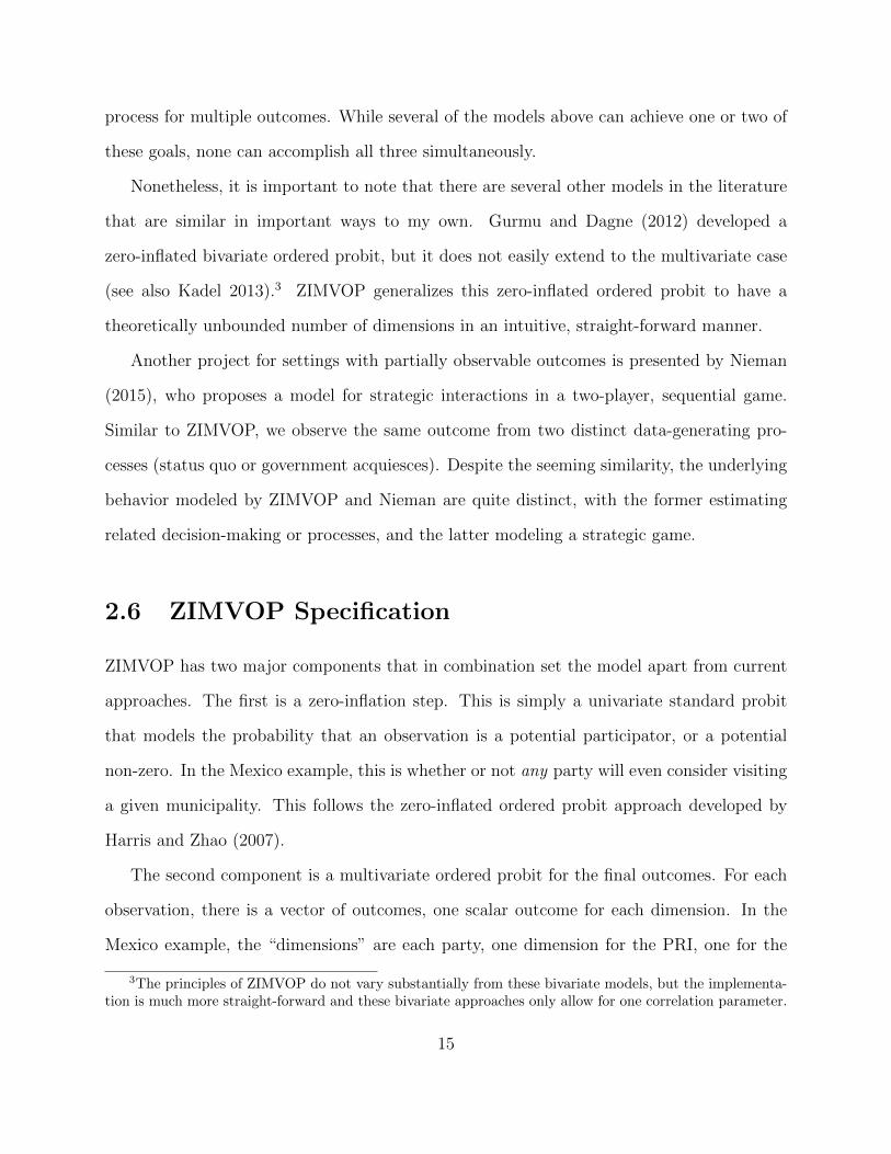
Despite the difficulty of the test, Figure 2.2 shows that across specifications, the model

accounting for the zero inflation performs better. The root mean squared error (RMSE),12 a

measure of bias and inefficiency, of the second-step estimates is smaller, while the standard

deviations, a measure of precision, of the posteriors are smaller. The average bias across

specifications is very close to zero for both models, suggesting that in the aggregate neither

has an expectation of bias, but, as shown by the relatively high RMSE, any given estimate

using the MVOP estimator is much less likely to be close to the true value of interest.

Further, the estimation of the correlation is much closer to the true values when modeling

the zero-inflation. If we have a substantive interest in the correlations, we will get very

10Although the coefficients are relatively large for a probit model, the large cut-offs across dimensionsensures a reasonable number of outcomes that are one or two. Nevertheless, I analyze a smaller set ofsimulations using smaller coefficients and smaller cut-offs, and another set increasing the noise to signalratio, and the improvements to the estimates hold. The choice of larger numbers for both the coefficientsand cut-offs was made out of convenience only.

11The first of every simulation set-up, for both the first and second set, were run for 10,000 iterations andtwo chains. All R’s were close to one and lack-of-convergence tests with the package superdiag indicatedno problems. The remaining were run for 20,000 iterations to make convergence likely without having totest for convergence on all models.

12RMSE is calculated by squaring the difference between the estimates and the true values and takingthe mean.

22

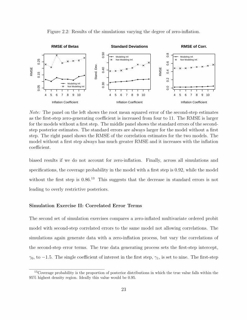
Figure 2.2: Results of the simulations varying the degree of zero-inflation.

4 5 6 7 8 9 10

0.05

0.15

0.25

RMSE of Betas

Inflation Coefficient

RM

SE

Modeling Inf.Not Modeling Inf.

4 5 6 7 8 9 10

0.30

0.40

0.50

Standard Deviations

Inflation Coefficient

Sta

nd. D

ev.

Modeling Inf.Not Modeling Inf.

4 5 6 7 8 9 10

0.0

0.2

0.4

0.6

0.8

RMSE of Corr.

Inflation Coefficient

RM

SE

Modeling Inf.Not Modeling Inf.

Note: The panel on the left shows the root mean squared error of the second-step estimatesas the first-step zero-generating coefficient is increased from four to 11. The RMSE is largerfor the models without a first step. The middle panel shows the standard errors of the second-step posterior estimates. The standard errors are always larger for the model without a firststep. The right panel shows the RMSE of the correlation estimates for the two models. Themodel without a first step always has much greater RMSE and it increases with the inflationcoefficient.

biased results if we do not account for zero-inflation. Finally, across all simulations and

specifications, the coverage probability in the model with a first step is 0.92, while the model

without the first step is 0.86.13 This suggests that the decrease in standard errors is not

leading to overly restrictive posteriors.

Simulation Exercise II: Correlated Error Terms

The second set of simulation exercises compares a zero-inflated multivariate ordered probit

model with second-step correlated errors to the same model not allowing correlations. The

simulations again generate data with a zero-inflation process, but vary the correlations of

the second-step error terms. The true data generating process sets the first-step intercept,

γ0, to −1.5. The single coefficient of interest in the first step, γ1, is set to nine. The first-step

13Coverage probability is the proportion of posterior distributions in which the true value falls within the95% highest density region. Ideally this value would be 0.95.

23

equation is therefore;

s∗i = −1.5 + vi × 9 + µi,

µi ∼ N (0, 1), and

si =

0 if s∗i ≤ 0,

1 otherwise.

The values of v, which is of length 500, are again all drawn from the standard normal for

each simulation, and each unique data set is analyzed by the competing models to ensure

comparability. The values of the predictors are generated independently of the second-step

values, which are generated as above, from a standard normal. They are not nested.

The second step has three outcome levels on each of three dimensions. The coefficients

used are the same as the earlier round of simulations. Intercepts are set to zero and the

parameters of interest are set to 2, 2.5, and 2. The outcomes generated however are deter-

mined using correlated error terms, with the correlation varying across simulations.14 The

second-step equation is:

zi = xi

2

2.5

2

′

+ εi,

εi ∼ N

0

0

0

,

1 ρ12 ρ13

ρ12 1 ρ23

ρ13 ρ23 1

.

Again, the cut-offs for every dimension are set to 0 and 2. These simulations are repeated

100 times each, resulting in 2,700 sets of data, analyzed once by each model.

14There are twenty-seven different data generating processes. The first nine set the second and thirdcorrelations, ρ13 and ρ23, to zero, and ρ12 varies from −0.8 to 0.8 by 0.2. The second nine keep the sameρ12 shift, setting ρ13 to ρ212 and ρ23 to ρ312. The final nine again maintain the same ρ12 shift and set ρ13 toρ12 and ρ23 = ρ212. This choice stemmed partly from the need to generate positive definite matrices. Thismeans that when the first correlation coefficient is large (positive), the others are also positive or zero, whilewhen it is small (negative), the other two are sometimes of opposite signs.

24

Figure 2.3: Results of the simulations varying correlations.

−0.5 0.0 0.5

0.08

0.12

0.16

RMSE

ρ12

RM

SE

Modeling Corr.Not Modeling Corr.

−0.5 0.0 0.5

0.88

0.92

0.96

Coverage Probability

ρ12

Cov

erag

e P

rob.

Modeling Corr.Not Modeling Corr.

−0.5 0.0 0.5

0.28

0.32

0.36

0.40

Standard Deviations

ρ12

Sta

nd. D

ev.

Modeling Corr.Not Modeling Corr.

Note: The panel on the left shows the root mean squared error of the second-step estimatesas the first correlation coefficient increases. The model allowing correlation performs betterby this metric. The middle shows the coverage probability of the second-step estimates, witha line at 0.95. The right panel shows the standard deviations of the posterior distributions.Despite the decent coverage of the model allowing correlations, the standard deviation of theposterior distribution is markedly smaller, performing best when the absolute correlationsare high.

Results of the exercise are shown in Figure 2.3, pooled by the first correlation coefficient.

Again, we see a smaller RMSE in the second-step estimates with tighter posteriors as shown

by the smaller standard deviations. The average bias across estimators is very close to zero,

but any given estimate is less likely to be close to the true value of interest if ignoring

the correlations in the error terms, as shown by the high RMSE. Despite the increase in

precision, the average coverage probability is still close to 0.95. Further, the ZIOP does not

produce correlation estimates, which are substantively interesting, for example to capture

the relationship between parties’ decisions.

When comparing the proposed model to both one not modeling the zero-inflation and

one not modeling correlations, the proposed model outperforms these currently extant al-

ternatives. Results hold across various specifications and different benchmarks. Overall, the

RMSE of the second-step estimates is reduced, and the posterior densities are more precise

while still maintaining approximately 0.95 coverage. ZIMVOP is more accurate, more effi-

25

cient, and produces substantively interesting results by modeling both the zero-inflation step

and the second-step correlations.

2.7.2 Application: Presidential Campaigns in Mexico

Having demonstrated the benefits to our inferences using ZIMVOP, I will now apply it to

presidential campaigns in Mexico. Langston and Rosas (2016) argue that municipal-level

party support and competitiveness are significant determinants to party campaigns’ calculi

when deciding which municipalities to visit, and whether that visit is a meeting or a rally.

Visits can help assess and signal local party strength and their mobilization networks, and

can signal a party’s interest in a locality. If they hold a rally and it is not well-attended,

however, this can impose more costs than benefits, signaling a lack of strength in the area.

Rallies are also expensive, and if the return is not great enough the cost is not worth it.

To test the saliency of certain factors entering into this decision, they analyze the Mexican

presidential campaigns of 2006 and 2012, focusing on the three major parties – the PRI, the

PAN, and the PRD, using a pooled zero-inflated ordered probit.

The current analysis builds on this with two main propositions: (1) the strategies of

parties are not the same and will respond to local support differently, and (2) the deci-

sions made by parties are related. Parties likely engage in a Colonel Blotto-type interaction,

targeting the municipalities their rivals are targeting,15 and their decisions are likely inter-

dependent based on unobservable characteristics as well. ZIMVOP is uniquely suited to test

these propositions because coefficient estimates vary between parties, and the correlation

between the parties’ decision processes captures the degree to which parties decisions are

related. This proposed relationship between the parties should result in a positive estimate

15The Colonel Blotto game, first solved by Borel (1921), is a game based on the idea that battlefieldswill be won by whichever side sends the most troops, causing a pooling of resources at locations. This ideahas been used as a metaphor for party competition in the political science literature (see Laslier and Picard2002; Myerson 1993).

26

of the correlation. Further, the vast majority of municipalities are never visited. To obtain

reliable estimates of the correlations between parties’ calculi and the coefficients of interest,

a zero-inflation step is necessary.

The outcome is a vector of ordered party outcomes – 0 for no visit, 1 for a meeting,

and 2 for a rally. There are three dimensions, one for the PRI, one for the PAN, and one

for the PRD. For example, if the PRI holds a meeting in a municipality at a given time

period, the PAN do not visit, and the PRD hold a rally, the outcome would be [1,0,2]. The

first-step predictors consist of one matrix of municipal characteristics. I use three variables:

Population size, Vote HHI, and 2012 dummy. The variable Population size is a measure of

how populated a municipality is. Sparsely populated municipalities are not worth a visit.

The variable 2012 dummy is a dummy variable indicating if the observation is in 2012 rather

than 2006. The visits are, according to Langston and Rosas (2016), a common strategy in

newer democracies that still have clientelistic networks. As a state’s democracy grows and

evolves, these visits should be less common. Finally, to capture competitiveness, I include

the HHI (Herfindahl-Hirschman) index of the previous vote as a general measure for party

dominance in the municipality. This measure is a sum of the squared previous vote shares

for each of the three parties. When it is high, it indicates one party has dominance over the

others. These municipalities should be less appealing for parties to visit. Either it is the

dominating party and there is little to be gained from a visit, or it is the weaker party and

going would be both a waste of resources and potentially damaging.

The second step includes all of the variables used in Langston and Rosas (2016), including

the first-step variables. Variables included that are not in the first step are Gira, Concurrent,

Coparty mayor, and Previous vote. The variable Gira is a dummy variable for whether or

not the visit was part of a multi-stop tour. The variable Concurrent is a dummy indicating

whether or not the mayoral race is concurrent with the presidential race. The two main

variables of interest are Coparty mayor, an indicator for whether or not there is a mayor

27

of the same party, and Previous vote, the party’s previous vote share. These capture the

underlying political support for a party. In the original data, if a party visits a municipality

more than once in a given time period it is included twice. For this analysis, to keep the

number of observations the same and to not falsely give parties 0 outcomes or repeated

outcomes, duplicates are dropped, keeping the highest outcome. This only affects about 150

out of over 3,000 observations. About half of the data are randomly selected municipalities

that were not visited by any party.

Analysis

The results of the analysis are presented graphically in Figure 2.4.16 There is strong evidence

for the two propositions. First, the correlation estimates are all positive and reliable. This

suggests parties are engaging in Colonel Blotto dynamics and targeting municipalities their

competitors also target, and that municipalities have unobserved attributes that make them

more or less attractive to parties. Second, the second-step estimates for the parties of the

variables of interest vary considerably. The estimates for Coparty mayor and Previous vote

vary across parties, suggesting different calculi for the parties.

For the PAN, having a mayor of the same party reliably increases the odds ratio of moving

up a category in the visitation scheme. It is unreliable for the PRI, but indicates that the

PRD may be responding to this in the opposite direction. The estimates for Previous vote

suggest something similar: parties are not responding in the same way to the same factors.

Again, the PAN seem to go where they have support, but so do the PRD, while the PRI

estimate, though (just barely) unreliable at a 95% level, suggests that the PRI is more likely

to visit and hold rallies in municipalities with less support.

Langston and Rosas (2016) find that Coparty mayor has a positive effect, while they fail

to reject the null that Previous vote has any effect. This is somewhat of an unfair comparison,

16Two chains of 150,000 iterations were run. The package superdiag indicated no evidence of lack-of-convergence, and all R’s are close to one.

28

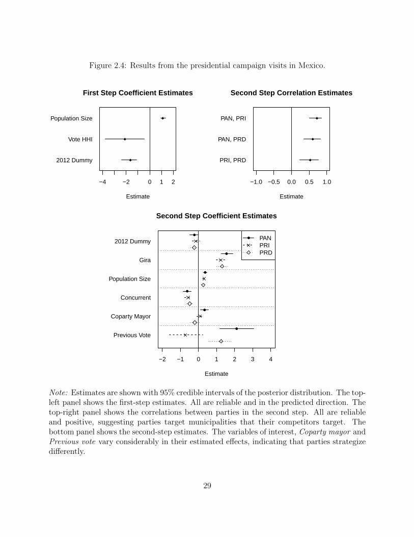
Figure 2.4: Results from the presidential campaign visits in Mexico.

−4 −2 0 1 2

First Step Coefficient Estimates

Estimate

2012 Dummy

Vote HHI

Population Size

−1.0 −0.5 0.0 0.5 1.0

Second Step Correlation Estimates

Estimate

PRI, PRD

PAN, PRD

PAN, PRI

−2 −1 0 1 2 3 4

Second Step Coefficient Estimates

Estimate

PANPRIPRD

Previous Vote

Coparty Mayor

Concurrent

Population Size

Gira

2012 Dummy

Note: Estimates are shown with 95% credible intervals of the posterior distribution. The top-left panel shows the first-step estimates. All are reliable and in the predicted direction. Thetop-right panel shows the correlations between parties in the second step. All are reliableand positive, suggesting parties target municipalities that their competitors target. Thebottom panel shows the second-step estimates. The variables of interest, Coparty mayor andPrevious vote vary considerably in their estimated effects, indicating that parties strategizedifferently.

29

as they test a generalizable pattern on pooled data, but at the same time this highlights the

advantage to allowing actors to respond to factors differently. Perhaps a fairer test is to

compare these results to a model not allowing correlation, but allowing the second-step

estimates to vary, as in the second simulation exercise. The first-step estimates are nearly

identical, but the second-step posteriors are fairly different, with the estimate for previous

vote of the PRI no longer reliable even at the 90% level. The second-step estimates from

both models are compared in the Appendix. Perhaps most importantly, we are losing the

ability to draw substantive conclusions from the correlations in the latter model. Further,

the simulation exercises suggest we should trust the posteriors from ZIMVOP.

2.8 Conclusion

Binary and ordered outcomes are often of interest in political science, but analyses of these

data can be problematic. There is often an excess of zeros, and the data generating pro-

cesses of seemingly unrelated outcomes may in fact be related. These issues can lead to

inaccurate and inefficient estimators. This chapter proposes a new extension to existing

models, ZIMVOP, that appropriately addresses these issues and in doing so opens the door

to answering questions we have been unable to answer. ZIMVOP not only provides better

estimates of our parameters of interest as shown in the simulation exercises, it also helps us

recover useful information that otherwise would be lost. We can investigate the nature of the

related processes causing observed outcomes and analyze the varying effects of observables

at the zero-inflation step and the outcome step. I applied ZIMVOP to presidential campaign

visits in Mexico to illustrate the model’s benefits.

Though ZIMVOP outperforms existing models in certain contexts, it is not as straight-

forward to interpret as its simpler alternatives. ZIMVOP is also fairly computationally

intensive, with some models taking a very long time to converge. Further, it only applies to

30

cases in which we believe processes are related and an excess of zeros suggests two steps of

data generation. Nevertheless, the applicability of ZIMVOP is potentially wide.

For example, decision-making often results in unanimity. During U.S. Supreme Court

agenda setting, most Justices vote to not hear the case. If we want to explain the likelihood

of SCOTUS accepting a case, there is very likely a relationship between the processes of

one Justice voting to hear the case and another Justice wanting to hear the case that is

unexplained from observables. This would in fact be a very interesting question because

some correlations, such as those of ideologically proximate Justices, may be positive, while

those of ideologically distant Justices may be negative. Survey questions are also a very well-

suited application of the model, with frequent pooling at “do not know” or “indifferent.”

Finally, ZIMVOP as proposed in this chapter has a zero-inflation step modeling the all-

zero state. In other words, though the outcome is multivariate, the zero-inflation step is

univariate. This is computationally less demanding and in general theoretically sensible.

There are municipal-level characteristics that make no municipality visitable, for example.

With this example, particularly when considering that the underlying processes are related,

there would be no reason to deviate from this univariate zero-inflation. However, ZIMVOP

could easily allow for inflation in each component, potentially opening up new avenues of

application.

31

Modeling Without Conditional

Independence: Gaussian Process

Regression for Time-Series

Cross-Sectional Analyses

In political science research, we frequently rely on the conditional independence assumption.

That is, potential outcomes are unconditional on our explanatory variable, conditional on

our covariates. Related, and perhaps more simply, we assume that our error terms are

independently and identically distributed. Yet it is well-understood that this assumption is

frequently violated.

These modeling and data features, representing violations to conditional independence,

are particularly prevalent in time-series cross-sectional (TSCS) and panel analyses. To ac-

count for these violations, the most common solution is to model the data-generating process

ignoring violations of conditional independence then correct the standard errors afterwards

to account for non-independence. These procedures, such as robust clustered standard errors

or panel corrected standard errors, have well-known problems, including biasing estimates

and standard errors and leading to incorrect inferences (Esarey and Menger 2017; King and

Roberts 2015).

32

In this chapter, I introduce Gaussian process regression (GPR) to political science as a

solution by which we directly model non-independence (Gibson et al. 2012; Gramacy and

Lee 2008; Rasmussen and Williams 2006; Gramacy 2005). GPR is a very flexible Bayesian

machine-learning algorithm that concurrently models the error distribution as a function of

the input space and the outcomes conditional on the covariates.

As a consequence of explicitly handling non-independence, GPR outperforms existing

alternatives in terms of bias, efficiency, and false positives and negatives in TSCS analyses.

GPR is also relatively insensitive to the common problems arising in real-world data analyses

including small cluster sizes or small intra-cluster sample sizes.

The outline of the chapter is as follows. First, I discuss the issues and current solutions to

TSCS analyses, highlighting the drawbacks and benefits of extant modeling strategies. Sec-

ond, I specify the GPR model, with some discussion of the theory and spirit of the approach.

Third, I apply the model, showing improvements to extant approaches through several sim-

ulation exercises. I then demonstrate that inflation in Latin America leads to improved

sentiment towards the United States, while other modeling strategies cannot reject the null

hypothesis of no effect. This exercise demonstrates that ignoring or improperly correcting

for violations of the conditional independence assumption may lead to false conclusions. It

also shows that the degrees of freedom lost by the most common strategies under-estimate

the causal impact of an explanatory variable on the outcome. In this subsection, I also

discuss issues of over-fitting, out-of-sample predictions, and model selection. I next replicate

Getmansky and Zeitzoff (2014), showing that the authors under-estimate the effect of terror

threats on right-wing votes in Israel. In the replication, different modeling strategies lead to

very different substantive results. This highlights the importance of model choice, and the

general under-estimation of the effect again demonstrates the potential issues that arise when

decreasing the degrees of freedom in the model. I conclude in the final section with future

directions. As part of this project, I provide Stan code as implemented in the R computing

33

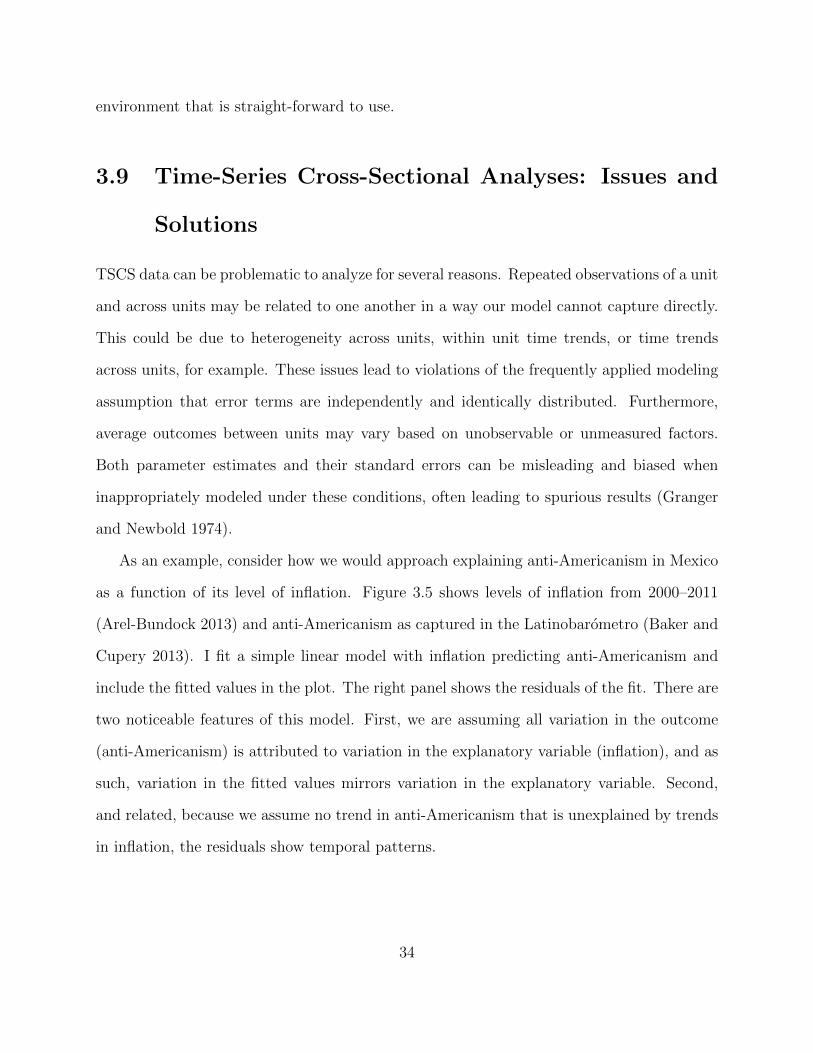
environment that is straight-forward to use.

3.9 Time-Series Cross-Sectional Analyses: Issues and

Solutions

TSCS data can be problematic to analyze for several reasons. Repeated observations of a unit

and across units may be related to one another in a way our model cannot capture directly.

This could be due to heterogeneity across units, within unit time trends, or time trends

across units, for example. These issues lead to violations of the frequently applied modeling

assumption that error terms are independently and identically distributed. Furthermore,

average outcomes between units may vary based on unobservable or unmeasured factors.

Both parameter estimates and their standard errors can be misleading and biased when

inappropriately modeled under these conditions, often leading to spurious results (Granger

and Newbold 1974).

As an example, consider how we would approach explaining anti-Americanism in Mexico

as a function of its level of inflation. Figure 3.5 shows levels of inflation from 2000–2011

(Arel-Bundock 2013) and anti-Americanism as captured in the Latinobarometro (Baker and

Cupery 2013). I fit a simple linear model with inflation predicting anti-Americanism and

include the fitted values in the plot. The right panel shows the residuals of the fit. There are

two noticeable features of this model. First, we are assuming all variation in the outcome

(anti-Americanism) is attributed to variation in the explanatory variable (inflation), and as

such, variation in the fitted values mirrors variation in the explanatory variable. Second,

and related, because we assume no trend in anti-Americanism that is unexplained by trends

in inflation, the residuals show temporal patterns.

34

Figure 3.5: Inflation and anti-Americanism in Mexico

(a) Data points and fitted values

2000 2002 2004 2006 2008 2010

45

67

89

10

Year

Infla

tion

Year

2.0

2.2

2.4

2.6

2.8

Ant

i−A

mer

ican

ism

Inflation (explanatory)Anti−Americanism (outcome)Fitted

(b) Residuals of model fit

2000 2002 2004 2006 2008 2010−0.

3−

0.1

0.1

0.2

0.3

Year

Res

idua

ls

Note: The left panel shows inflation in Mexico (green dots), anti-Americanism in Mexico(blue triangles), and fitted values of a linear model (black x’s) with inflation explaininganti-Americanism. The right panel shows the residuals of the model. Trends in the outcomeare assumed to mirror trends in the explanatory variable, yet the residuals demonstrate thatthere is likely a trend in the outcome unexplained by trends in the explanatory variable.

Common modeling approaches ignore the violations to the conditional independence as-

sumption and adjust the standard errors afterwards, allowing for clustering at the unit of

observation. Serial correlation of observations within units may also be accounted for through

an autoregressive framework. Fixed effects may be employed both as a way to adjust the

standard errors and account for heterogeneity of the units. Alternatively, random effects

serve a related purpose in multilevel modeling approaches. Unfortunately, there is no best

practice, as every data set is unique. In this section I discuss the advantages and disadvan-

tages of the more common, although by no means exhaustive, strategies used in political

science research, after a brief review of current practice.

35

3.9.1 Prevalence of Current Approaches

I reviewed all time-series cross-sectional articles17 in the last three years18 from American

Political Science Review, American Journal of Political Science, Journal of Politics, and

Comparative Political Studies, noting the strategies employed to deal with the data. Of

the 320 TSCS articles reviewed, 82 run a model with group and time fixed effects (FE),

47 with only a group fixed effect, and 25 with only a time fixed effect.19 48 articles use

random effects (RE) modeling strategies. 172 articles use robust clustered standard errors

(RCSE), 17 use panel corrected standard errors (PCSE), and one uses Newey-West standard

errors. 23 lag one or more dependent variables (LDV). 17 use some time trend specification.

Finally, one article uses a first differences approach. Based on the prevalence, I will discuss

and compare GPR to FE with RCSE, PCSE, and LDV, and to RE specifications, the most

common strategies.

3.9.2 Fixed-Effects Specifications

Fixed-effects (FE) regressions are often used when the researcher believes there is heterogene-

ity in baseline outcomes across groups, and this heterogeneity is based on omitted variables

that are correlated with included regressors (Greene 2003, p. 359). Essentially, a different

intercept is estimated for each unit. Specifically, let i index units, y be a vector of outcomes,

X be a matrix of covariates, and β our estimand. The group fixed-effect models the data

according to:

y = γ + Xβ + ε, (3.1)

17Models such as survival or hazard models are not included in this discussion.18The end date is July 2017.19Note that articles often use a mixture of strategies in different models, so the number will not sum to

the total, 320.

36

where γ is a vector of the unit-level intercepts for each unit i.

There are a few major drawbacks to this general modeling strategy. First, for the iden-

tification of the covariance matrix within-group variation of the data is required (Greene

2003, p. 362). If there is little variation of the explanatory variable the results of the model

are not asymptotically unbiased or efficient. If there is no variation in a given variable, the

effect cannot be estimated at all (Greene 2003, p. 360). Second, this method is only con-

sistent in large data sets. In other words, while consistent asymptotically, we often have to

analyze relatively small data sets and the method may produce misleading results in these

situations (e.g., Esarey and Menger 2017). Fixed effects models also rely on the assumption

that a unit’s error term and the constant capturing the unit’s unique characteristics are not

correlated with other units (Greene 2003, p. 359).

In addition to including a fixed effect for each group, it is also common to include a fixed

effect for each time period in TSCS analyses. We estimate a separate intercept for each

group and for each time period, indexed by t. We then model the data according to:

y = γ + τ + Xβ + ε, (3.2)

with τ the vector of time-specific intercepts for each time t.

We might consider a model of this sort if we believe there are confounders across time

experienced equally by every unit, again correlated with our variables of interest. While

the goal is to allow for time effects, the same effect is assumed for each unit, which is often

unrealistic. For example, returning to the question of inflation in Latin America, Figure 3.6

shows inflation in four Latin American countries from 2000–2011, with the posteriors of a

fitted two-way fixed effects model.

37

Figure 3.6: Two-way fixed-effects model fit and residuals of inflation in Latin Americancountries over time

(a) Model fit

2000 2002 2004 2006 2008 2010

05

1015

2025

30

Year

Infla

tion

VENURYGTMPER

(b) Residuals of model

2000 2002 2004 2006 2008 2010

−6

−4

−2

02

46

8

Year

Res

idua

ls

VENURYGTMPER

Note: Displayed in the left panel are actual inflation in four Latin American countries,Venezuela, Uruguay, Guatemala, and Peru, from 2000–2011 with a 50% linear fixed-effectsposterior of the observations. The only information in the model is an indicator for thecountry and a continuous time variable. The right panel shows the residuals of the fit.

Unrealistically, the trend for each country is assumed to be the same, leading to poor

model fit, with only their averages, i.e. group-level intercepts, allowed to vary. Further, as

seen in the residiual plot in the right panel, there are time trends in the residuals within

countries, and because each year is essentially averaging the “effect” of time, the residuals

are not independent, but instead mirror other countries. If the residual of one country is

high, the others necessarily must be lower on average.

In addition to these issues, the substantial cost in terms of degrees of freedom in the

two-way FE model is often not justified, and the model ignores timewise evolution. Time

effects are unlikely independent from the previous time effect, for example, but this is ignored

with the modeling strategy (Greene 2003, p. 364). In addition, these models can accentuate

problems of multicollinearity among regressors (Baltagi 2008, p. 35).

38

3.9.3 Random-Effects Specifications

Fixed-effect regression can be thought of as applying only to the units in the study, not

out-of-sample units. This both means the strategy does not allow out-of-sample inference,

and more theoretically assumes the population being studied is complete. In this case it is

reasonable to assume the model is constant (Greene 2003, p. 370). Alternatively, we can

model the individual constant terms as randomly distributed across units (Greene 2003, p.

371).

This modeling strategy, known as random effects (RE) regression, is only appropriate

if the omitted unit effects are uncorrelated with the regressors, and the sampled units are

drawn from a large population. Random effect estimation reduces the number of parameters

to be estimated, allows for time-invariant predictors, and allows for out-of-sample inference.

However, if the assumptions are not valid, the estimators are inconsistent (Greene 2003;

Mundlak 1978). Further, while the specification allows disturbances to be correlated within

groups, it does not allow for a correlation between groups. As with fixed effects, random

effects can be estimated for group and/or time.

To determine whether FE or RE is more appropriate given the data, the most common

test is Hausman’s specification test (Greene 2003; Hausman 1978). However, this test has

been criticized for assuming the RE model as the null (Baltagi 2008, p. 65–73), and has

been shown to perform poorly under certain violations to the underlying assumptions, with

no clear alternative (Esarey and Jaffe 2017).

3.9.4 Clustering Standard Errors

Clustered standard errors are most common when coupled with a fixed effects model. Clus-

tering the error terms allows for dependency of the residuals within units. The most widely

used variants of clustering standard errors is the modification of robust standard errors

39

(White 1980) to allow for clustering, known as robust clustered standard errors (RCSE)

(Cameron, Gelbach, and Miller 2011). Although consistent in various situations (Liang and

Zeger 1986), the use and prevalence of RCSE has been criticized for leading to false positives

and negatives when the number of units is small (Esarey and Menger 2017). Further, King

and Roberts (2015) argue that when robust standard errors and the maximum likelihood

standard errors diverge, this is evidence that the model is misspecified, suggesting their use

should be limited to testing specification problems (see also Tauchen 1985; Newey 1985;

White 1982). There is often a divergence of the two in the presence of serial correlation

(Cameron and Miller 2015), suggesting that serial correlation can lead to a misspecified

model.

Another clustering alternative is panel corrected standard errors (PCSE) (Beck and Katz

1995). PCSE are derived with the expectation that errors are serially correlated within units

and correlated between units at a given time. It is a method for computing a heteroskedastic-

consistent covariance matrix specifically for TSCS data. Again, this method is frequently

coupled with fixed effects when the researcher believes each unit has a different baseline

outcome, and the errors are clustered within units. This method also relies on a large

number of units, and can lead to very misleading results when the number of units is small,

with no general rule-of-thumb as to how small a number is inappropriate for this strategy.

Further, when the errors are correlated with a regressor the standard errors can become

much larger than desired (Cameron and Miller 2015). Finally, this two-way clustering does

not pick up on all potential correlations in the data (Cameron and Miller 2012).

As outlined in Esarey and Menger (2017), there are other, more exotic clustering strate-

gies in the statistics literature that are largely absent from the political science literature.

For example, cluster-adjusted t-statistics (CATs) (Ibragimov and Muller 2010), wild cluster

bootstrapped t-statistics (WCBSTs) (Cameron, Gelbach, and Miller 2008), and pairs cluster

bootstrapped t-statistics (PCBTs) (Cameron, Gelbach, and Miller 2008) are all clustering

40

alternatives. However, like in Esarey and Menger (2017), preliminary simulation exercises

demonstrated that more traditional approaches out-perform these less-known clustering op-

tions.

3.9.5 Correcting for Serial Correlation

Serial correlation in the outcome can be either due to serial correlation of the error terms,

in other words the outcome itself, or due to serial correlation of an explanatory variable.

Ignoring the correlation can lead to very misleading results (Granger and Newbold 1974).

Although PCSE corrects for serial correlation in the error terms, RCSE has no temporal

component, nor does a varying-intercept multilevel model. However, adjustments, such

as Newey-West standard errors (Newey and West 1987; Andrews 1991), can account for

serial dependence in the error terms in static data-generating processes. If a dynamic data-

generating process is suspected, lagging the dependent variable can account for both serial

correlation and the underlying dynamics (Beck 1985). These models, however, perform

poorly when the process is static or weakly dynamic, or the dependent variable is non-

stationary (Keele and Kelly 2005). In the latter case, modeling first differences or including

time trends may alleviate some of the issues, but these do not handle breaks in the trends

well. Further, these approaches assume a sequential data-generating process, ignoring the

possibility of endogeneity and an effect of anticipation. I will now discuss GPR as an alter-

native modeling choice for TSCS data and compare GPR to these most common strategies.

3.10 Gaussian Process Regression for TSCS Data

GPR is primarily known for its uses in machine learning classification and prediction (Ras-

mussen and Williams 2006), but the models have been utilized to make inferences about

populations as well (e.g., Kirk and Stumpf 2009; Huang, Zhang, and Scholkopf 2015; Garg,

41

Singh, and Ramos 2012; Qian, Zhou, and Rudin 2011; Gibson et al. 2012). Monogan and

Gill (2016) use a GPR approach, which they refer to as Bayesian kriging, to estimate a

posterior density blanket of citizens’ ideologies across the United States. Despite having rel-

atively sparse data, the method allows for any level of geographic aggregation and provides

an estimate, with uncertainty, of the ideology of the region by smoothing across space.

This smooth blanket over the U.S. is a useful introduction to conceptualize GPR. Data, in

Monogan and Gill (2016) a measure capturing ideology, are not conditionally independent.

The average ideology in a town is likely similar to the ideology in its neighboring towns

even conditional on covariates. We can consider these outcomes (ideology in neighboring

towns) as coming from a joint normal distribution if we assume each realization comes from

a separate normal distribution, with the outcomes sharing a correlation.

The mean of the multivariate normal can be parameterized allowing for standard infer-

ences on parameters of interest, i.e., how changes in an explanatory variable correlate with

changes in a dependent variable. The variance-covariance matrix is similar to kernel regu-

larized least squares (Hainmueller and Hazlett 2013), but different in that the approach is

fully Bayesian. This allows estimation of a much more flexible variance-covariance matrix

in a kernel with weakly informative priors rather than setting the tuning parameters, and

provides a posterior of variance-covariance matrices through MCMC. The effect of a variable

on an outcome is also not easily interpretable in KRLS, whereas the sampled mean in GPR

provides easily understood posteriors of our parameters of interest.

The “smoothing” across geographic space is intuitive, but in reality we can smooth over

any input dimension we choose, including, of course, time. The same way neighboring towns

are likely heavily correlated, so too are temporally proximate observations, or observations

sharing similar explanatory variables. These correlations can also vary from dimension to

dimension. In other words, geographic proximity and temporal proximity need not share

the same correlation. Rather than considering data as independent, or even sequential, we

42

can think of all observations as coming from one joint distribution, with data points close

to each other in the covariate space likely similar. The flexibility of the model makes it

ideal for modeling situations in which there are violations of the conditional independence

assumption but the degree of these correlations is not known a priori.

These features of GPR make the model uniquely suited to deal with TSCS data. Se-

rial correlation within units and across units, between unit heterogeneity, and correlations

between unit-level averages (i.e., intercepts) and unit-level explanatory variables can all be

accounted for in the learning kernel and the parameterization of the mean function. Per-

haps most importantly, we do not require heroic assumptions about the nature of these data

features, unlike the most commonly applied approaches.

To continue with the example of inflation, Figure 3.7 shows the same inflation data as

Figure 3.6 in four Latin American countries over time, with posterior predictive distributions

generated with GPR using only a dummy variable for the country and a linear measure of

time. Rather than model the outcomes with typical distributional assumptions where errors

are assumed to be independent and identically distributed, all errors are modeled jointly as

coming from a multivariate normal distribution that explicitly allows for non-independence

between observations. The variance-covariance matrix is learned from the data, smooth-

ing the posterior over the input space. As can be seen in the figure, the posteriors track

the outcomes very well, and GPR provides reasonable predictions even where there are no

covariates. Further, despite the flexibility, standard inferential techniques are still straight-

forward. GPR provides estimates of the posterior distributions of the parameters of interest

in a fashion similar to any Bayesian model.

3.10.1 GPR Specification

Now that I have explained the intuition behind the model, I will fully specify the TSCS GPR

model, both for completeness and to further aid in the intuition. We would typically assume

43

Figure 3.7: GPR fit of inflation in Latin American countries over time

2000 2002 2004 2006 2008 2010

05

1015

2025

30

Year

Infla

tion

VENURYGTMPER

Note: Displayed are actual inflation in four Latin American countries, Venezuela, Uruguay.Guatemala, and Peru, from 2000–2011 with a 50% GPR predictive posterior of theobservations. The only information in the model is an indicator for the country and acontinuous time variable.

44

a data generating process of observations in a linear model according to:

yi ∼ N (xiβ, σ2), (3.3)

with xi a vector of covariates for observation i and σ2 a scalar of the variance for all ob-

servations. However, with GPR, we assume a multivariate normal distribution modeling all

outcomes jointly. Specifically, the vector of outcomes, y, is distributed:

y ∼MVN (Xβ, σ2Ω). (3.4)

In Equation 3.4, the mean is still a linear function of the covariate space, but because

it is a multivariate normal the input is the entire covariate matrix for all observations, X.

This covariate matrix includes unit indicators (akin to fixed effects) to account for unit

heterogeneity. The linearity of the mean function allows for posterior inferences on our

parameters of interest (β), while allowing the kernel Ω to learn the complex underlying

data-generation from the data itself.

I deviate from previous implementations of the Gaussian process by allowing the data

used in the mean function to be different from the data used in the kernel. For TSCS pur-

poses, the kernel includes all covariates, including unit indicators, and includes a continuous

time input. Time is not included in the mean function, as we have no interest in the effect

of time, but we want to smooth over this dimension to account for time trends within and

between units.

In order to smooth over our covariate space, we want observations that are close in the

covariate space to share a correlation, while points further in the covariate space to share less

correlation. Therefore, we sum the squared distances across input columns. We then take

45

the exponential of the negative sum to capture the correlation. Let m indicate the number of

columns of the input matrix to the kernel, and let p index these columns in the summation.

Also let j and i indicate two observations. We start with setting the correlations according

to:

Ω(xj,xi) = exp

−

m∑p=1

(xpj − xpi)2. (3.5)

However, we want time one and time two to perhaps have a different correlation than

location one and location two, for example. For this purpose, we introduce another parameter

to the kernel, ζ, a vector learned from the data that estimates the degree of correlation

relative to distance for each dimension. The kernel then becomes:

Ω(xj,xi|ζ) = exp

−

m∑p=1

(xpj − xpi)2

ζp

, (3.6)

which is a symmetric matrix with all diagonal elements equal to one, because the sum of

the distance of the covariate space will be zero for elements that are identical, and all off-

diagonal elements represent a correlation. However, to ensure the matrix is non-singular, we

add a small constant to the diagonal elements. This is necessary because points very close

in the covariate space will have almost one in the kernel matrix, and this leads to numerical

instabilities. This is called the nugget.

To distinguish between inputs to the mean and inputs to the kernel, allow X to indicate

inputs to the mean and X∗ to indicate inputs to the kernel. The fully specified model is

therefore:

46

y ∼MVN (Xβ, σ2Ω), (3.7)

Ω(x∗j ,x∗i ) = Ω†(x∗j ,x

∗i ) + δgj,i, (3.8)

gi,j =

1 if j = i,

0 otherwise.(3.9)

Ω†(x∗j ,x∗i |ζ) = exp

−

m∑p=1

(xpj − xpi)2

ζp

. (3.10)

This kernel is known as the separable-exponential kernel. Other choices are possible (e.g.,

Rasmussen and Williams 2006, Ch. 4), but are left out for simplicity in the presentation.

The intuition is that the closer the inputs are in the hyperplane, the more correlated the

observations will be. However, each dimension has a separate estimate of the ζ parameter,

a scaling of the degree of correlation. The vector ζ is estimated in the learning resulting in

a posterior distribution. Now that the model is specified, I will discuss the priors used in

estimation.

3.10.2 Priors

The choice of priors comes from a combination of computational efficiency, a lack of prior

information, and constraints on the parameters. Other choices can be made, and inferences

from simulation exercises are not sensitive to the choices. However, scaling variables is

recommended if the scales are very different, or priors should be adjusted. The nugget, δ,

needs to be greater than zero. Let δ ∼ Exp(1) to ensure a positive term with weak prior

information that it would not be sensible for it to be too large, as that would lead to a poorly

fitting model. The nugget is only meant to allow the matrix to be non-singular, and large

values would add noise around data points that is already accounted for by the variance σ2.

47

The individual ζ terms also need be greater than zero, and we wish to be non-informative

as to whether a given dimension has a wavy or smooth surface (Gramacy and Lee 2008). As

such, we let each ζ be a mixture of gamma distributions, ζp = ζp1+ζp22

with ζp1 ∼ G(1, 20)

and ζp2 ∼ G(10, 10), giving roughly equal weight to parameterizations of wavy and smooth

populations.

I set the variance that pre-multiplies the kernel to have an inverse-gamma prior distri-

bution, σ2 ∼ IG(1, 1), again to be fairly non-informative, and to ensure a positive term.

Finally, β has a diffuse normal prior, specifically βiid∼ N (0, 3). Hyperpriors can be set, for

example the variance of the β’s, however this slows down estimation with no discernible gain

in inferences. I fit the model using Hamiltonian MCMC in Stan (Carpenter et al. 2016)

through the R package RStan (Stan Development Team 2016).

3.11 Applying GPR

I now apply GPR to simulated data to demonstrate its benefits. After validating the method

through the simulation results, I analyze the effect of inflation on anti-Americanism in Latin

America. I find that inflation decreases anti-American sentiment, but competing models

are unable to reject the null. I then replicate and expand upon Getmansky and Zeitzoff

(2014), showing that the threat of terror has a positive effect on right-wing voting, but the

effect is under-estimated in the original analysis and when applying the competing models.

Both applications show that modeling choice has a substantive impact on our conclusions,

and that over-specifying the models and decreasing the degrees of freedom decreases the

explanatory power of an independent variable. Further, there are likely issues with extant

approaches due to small sample sizes, serial correlation, and more.

48

3.11.1 Implementation on Simulated Data

In this section, I compare the results from GPR to those from the most common approaches to

handling time-series cross-sectional data under situations with problematic data-generating

processes. Specifically, I compare GPR to regressions using group and time fixed effects

using RCSE, PCSE, and lagging the dependent variable (LDV), and random effects models

using group and time effects (RE). GPR outperforms these extant alternatives when there

is serial correlation in the explanatory variable and the error terms within units, when there

is correlation between the explanatory variable and the unit-level intercept, when there is

correlation between an unrelated variable and the unit-level intercept, and when the number

of units or observations within a unit is small. GPR performs at least as well as the extant

alternatives even when these issues are less prevalent. In most circumstances, the estimator

is more efficient, less biased, produces better coverage probabilities, and produces fewer false

positives and negatives.

Serial correlation in error terms and explanatory variable within groups

A very common characteristic of time-series cross-sectional analyses is the existence of serial

correlation in the explanatory variable (e.g., inflation at time t in a country is correlated with

inflation at time t − 1). Serial correlation also commonly exists in the dependent variable,

or the error terms (e.g., anti-Americanism at time t in a country is correlated with anti-

Americanism at time t − 1). These correlations over time may arguably be unrelated to

other variables, but simply trends that are not easily captured without heroic assumptions.

GPR is well-suited to modeling these data relative to extant alternatives, because the

correlation matrix smooths over the input dimensions with minimal assumptions about the

degree of these correlations. To demonstrate the GPR benefits, I simulate data from a simple

process for 15 units at 15 points in time (n = 15 × 15 = 225), varying the level of serial

correlation within the units in 10 separate processes.

49

Specifically, the main explanatory variable, x, at time t = 1 is generated from an inde-

pendent standard normal across units. Subsequent x values are generated from a Markov

chain within each group, with the correlation ranging from ρ = 0.0 to ρ = 0.9 by 0.1. All

x’s are generated according to:

xi,t = ρxi,t−1 +√

1− ρ2F, (3.11)

with F representing a draw from the standard normal distribution. The generation of the

error terms, ε, follows the exact same procedure as the generation of x. The outcome, y, is

simply generated as:

y = 2 + x + ε. (3.12)

Each of the 10 processes is repeated 100 times, resulting in 1,000 analyses.

To visualize the simulated data, Figure 3.8 shows one unit over time when the serial

correlation is equal to 0.9. Note that this does not appear unrealistic data, especially when

considering the earlier real-world examples, and this is the highest level of serial correlation

simulated.

As the serial correlation increases, all models decrease in performance, but the GPR

outperforms them all easily. Figure 3.9 shows the average coverage probabilities and the

mean squared errors of the estimates as serial correlation increases. All models always

correctly identified x as having an effect distinguishable from zero at the 0.95 level, but

they do not capture the true parameter of interest as correlation increases, as shown by the

low coverage probabilities, and they have higher mean squared errors. The mean squared

errors of the lagged dependent variable model become too large to show graphically and still

50

Figure 3.8: Example simulated serial correlation data, ρ = 0.9

2 4 6 8 10 12 14

−2.

0−

1.5

−1.

0−

0.5

Time

x

0.0

0.2

0.4

0.6

0.8

1.0

y

xy

Note: This is one example of a unit in the serial correlation exercise, when the degree ofcorrelation equals 0.9. There is serial correlation in the explanatory variable (x) and serialcorrelation in the outcome (y) that is due both to the explanatory variable’s trend and itsown time trend.

compare the other competing models.

Correlation between the main explanatory variable and the group intercept

Another common problem with time-series cross-sectional analyses is the possibility of a

correlation between the main explanatory variable within a unit and the unit intercept. For

example, the average level of anti-Americanism within a country may be correlated with the

average level of inflation. This makes inferences regarding how changes in the explanatory

variable within a group impacts changes in the outcome particularly difficult. In this exercise,

I again vary the level of correlation of simulated explanatory variables and the unit intercept

and compare the performance of GPR to the most common modeling strategies.

I simulate 15 units with 15 observations (time points) per unit. For each unit, an inter-

cept, γi, is generated independently from the standard normal distribution. The explanatory

variable, x, is generated with a correlation again ranging from ρ = 0.0 to ρ = 0.9 by 0.1:

51

Figure 3.9: Results of simulations with varying degrees of serial correlation in error andexplanatory variable

(a) Average coverage probabilities

0.0 0.2 0.4 0.6 0.8

0.0

0.2

0.4

0.6

0.8

1.0

Correlation

Cov

erag

e pr

obab

ility

0.95

GPRRCSEPCSELDVRE

(b) Mean squared errors of estimates

0.0 0.2 0.4 0.6 0.8

0.00

50.

010

0.01

50.

020

Correlation

MS

E

GPRFELDVRE

Note: The left panel shows the average coverage probabilities across models as serial corre-lation increases with a dashed line at the ideal 0.95 level. The right panel shows the meansquared errors. GPR outperforms the most common modeling strategies by these metrics.

xi = ργi +√

1− ρ2F, (3.13)

where F are draws from a standard normal. The error terms, ε, are generated independently

from the standard normal. The outcome, y, is generated:

yi = γi + 0.35xi + εi. (3.14)

As before, each process is repeated 100 times for a total of 1,000 simulations.

The random effects model has the best true positive rates across simulations, almost

always estimating a reliable effect of x on the outcome. GPR is second best, modestly

outperforming the various fixed effects models. However, the random effects model has a

very poor coverage probability and a very high mean squared error relative to the other

52

models as the correlation increases. This is shown graphically in Figure 3.10.

Correlation between an unrelated variable and the group intercept

Perhaps a more problematic situation is when there exists a variable in the model that is

correlated with the unit intercept but has no effect on the outcome, as this can potentially

lead to false positives. In this simulation exercise, I generate unit intercepts γ from a

standard normal for 15 units, and generate 15 observations per unit, x, from the standard

normal. I also generate a vector of disturbances, ε, from the standard normal. The outcome

is then generated according to:

y = γ + .25x + ε. (3.15)

However, we model the data-generating process with an additional variable, z, that is cor-

related to the unit intercepts γ at ρ = 0.0 to ρ = 0.9 by 0.1. Specifically, I generate the

unrelated variable according to:

z = ργ +√

1− ρ2F, (3.16)

where F are draws from the standard normal. The assumed data-generating process is

therefore:

y = γ + xβ1 + zβ2, (3.17)

53

Figure 3.10: Results of simulations with varying degrees of correlation between group inter-cept and explanatory variable

(a) True positive rates across models

0.0 0.2 0.4 0.6 0.8

0.5

0.6

0.7

0.8

0.9

1.0

Correlation

True

pos

itive

rat

e

GPRRCSEPCSELDVRE

(b) Average coverage probabilities

0.0 0.2 0.4 0.6 0.8

0.4

0.6

0.8

1.0

Correlation

Cov

erag

e pr

obab

ility

0.95

GPRRCSEPCSELDVRE

(c) Mean squared errors across models

0.0 0.2 0.4 0.6 0.8

0.02

0.04

0.06

0.08

0.10

Correlation

MS

E

GPRFELDVRE

Note: The top-left panel shows the true positive rates. The top-right panel shows coverageprobabilities across models as the correlation of the intercept and explanatory variableincreases, with a dashed line at 0.95. The bottom panel shows the mean squared errors ofthe estimates. While the random effects model has the best power as shown by the truepositive rates, it also has the largest mean squared error and smallest coverage probability.GPR is on par with the other models, but mildly better at true positive rates.

54

Figure 3.11: False positive rates across models

0.0 0.2 0.4 0.6 0.8

0.0

0.2

0.4

0.6

0.8

Correlation

Fals

e po

sitiv

e ra

te

GPRRCSEPCSELDVRE

Note: As the correlation between the unit intercept and a variable unrelated to theoutcome increases, false positive rates stay low with the exception of the random effectsmodel.

and we are interested in whether we incorrectly estimate z as having an effect on y. In other

words, we should not be able to reject the null that β2 = 0. Again, each set-up is run 100

times for a total of 1,000 simulations.

All coverage probabilities, true positive rates, and mean squared errors of the effect of

x on the outcome are very good across all specifications, as there were no issues in that

variable. The false positive rates, that z is estimated as reliably affecting the outcome, are

good across all specifications except for the random effects models, which have very high

false acceptance rates. This is shown in Figure 3.11.

Varying the number of observations and number of units

Esarey and Menger (2017) find that modeling choices of TSCS data should in part be based

on the number of units. In this exercise, I vary the number of units and the number of

observations per unit when there is serial correlation as in the first exercise and when there

is a correlation in the explanatory variable and the unit intercept as in the second exercise.

Both of these issues are very common in TSCS data, and in comparative research in particular

55

we may not have the luxury of a large dataset. It is important, therefore, to analyze the

competing models’ properties at different amounts of data.

To achieve this, I simulate data sets, varying the number of units from five to 20 by five

and the number of observations in a unit from five to 20 by five. This results in data sets

that are 5× 5, 5× 10, . . . , 20× 20. Each data set is generated identically, only changing the

number of observations and units.

Group intercepts, γ, are generated independently from the standard normal distribution.

To create serial correlation in the x variable within units, the x is generated according to

Equation 3.11, setting the correlation, ρ, to 0.5. This is then added to 1.5 times the group

intercept to generate a serially correlated variable that is also correlated with the group

intercept. Finally, the error terms are generated according to Equation 3.11 as well. The

outcome is generated:

y = γ + 0.5x + ε. (3.18)

Each simulation set-up is repeated 100 times for a total of 1,600 simulations.

The results of the exercise are shown in Figure 3.12. The first column pools the results of

the data set by the number of units varying from five to 20. The first data point, for example,

shows the results when there are five units, and the number of observations per unit is five,

10, 15, and 20. The second column does the same but pools on number of observations in a

unit.

Because the data are problematic, and the average data set in any point is relatively small,

the coverage probabilities are fairly low, with the random effects model very low. However,

the random effects model has the highest true positive rate, but as demonstrated above this

56

Figure 3.12: Results of simulations with varying number of units and observations per unit

(a) Average coverage probabilities

5 10 15 20

0.4

0.5

0.6

0.7

0.8

0.9

Number of units

Cov

erag

e pr

obab

ility

GPRRCSEPCSELDVRE

(b) Average coverage probabilities

5 10 15 20

0.4

0.5

0.6

0.7

0.8

0.9

Number of observations in a unit

Cov

erag

e pr

obab

ility

GPRRCSEPCSELDVRE

(c) True positive rates

5 10 15 20

0.65

0.75

0.85

0.95

Number of units

True

pos

itive

rat

e

GPRRCSEPCSELDVRE

(d) True positive rates

5 10 15 20

0.6

0.7

0.8

0.9

1.0

Number of observations in a unit

True

pos

itive

rat

e

GPRRCSEPCSELDVRE

(e) Mean squared errors of estimates

5 10 15 20

0.02

0.04

0.06

0.08

Number of units

MS

E

GPRFELDVRE

(f) Mean squared errors of estimates

5 10 15 20

0.02

0.06

0.10

0.14

Number of observations in a unit

MS

E

GPRFELDVRE

Note: The first column pools on number of units and shows how the models perform as thenumber of units increases. The second column pools on the number of observations in aunit and shows performance as the number of observations (time periods) increases.

57

is generally at the expense of potential false positives under similar conditions. The mean

squared errors are also highest for the random effects model, and GPR outperforms all other

models at the true positive rate and has the lowest mean squared error of the estimates.

These simulation exercises have demonstrated that, under common issues plaguing TSCS

data, GPR outperforms the most widely applied extant models. In general, GPR leads to

fewer false positives and negatives, is a more efficient estimator, and decreases the error of

the estimate. These results are even more pronounced when the sample size is low. Having

demonstrated the benefits of GPR under common TSCS data characteristics, I will now apply

the model to better understand the relationship between inflation and anti-Americanism in

Latin America.

3.11.2 Application: The Effect of Inflation on Anti-Americanism

in Latin America

While GPR performs well across an array of metrics, it is important to understand how

our modeling choice impacts our substantive conclusions, the goal of quantitative research

in political science. It is also important to investigate the potentially deleterious effect of

making an inappropriate modeling decision. To show the differences in conclusions drawn

from different models, I apply the same models from the simulation exercises to a novel

substantive question regarding inflation and anti-Americanism in Latin America.

Do Latin American citizens blame the United States during periods of economic hardship,

or do they value the U.S. as a potential avenue to better their economic situation? I argue

that the latter is a more common reaction in the region. Specifically, as inflation, one

of the most meaningful indicators of economic hardship in Latin America, increases, anti-

Americanism will decrease. Or, in other words, pro-Americanism will increase.

Baker and Cupery (2013) find that economic exchange with the United States increases

58

sentiment towards the U.S. in Latin America, arguing that citizens of the region see the

economic hegemon as a source of material wellbeing and a destination for exports and emi-

grants (see also Weiss, Arguello, and Arguello 1995). In addition, there is empirical evidence

that economic integration with the United States benefits Latin American citizens (Florensa,

Marquez-Ramos, and Recalde 2015), and that Latin American citizens are distinctly in favor

of trade openness and economic integration (Baker 2003; Milner and Kubota 2005). Because

of this, it is reasonable to expect that a citizen facing lower purchasing power would increas-

ingly value the wealth that relations with the U.S. provide. When they are relatively well-off,

on the other hand, they will see less value in the economic effects of U.S. economic relations

and focus more on its foreign policy, which unsurprisingly is generally viewed negatively

(Fonseca 2008).

Data

To test the proposition, I utilize the question on the Latinobarometro20 used by Baker and

Cupery (2013), asking respondents their opinion of the U.S. Following Baker and Cupery

(2013), I average the responses from the representative sample in each country from 1995–

2011 to obtain yearly estimates of the dependent variable, Anti-Americanism. 18 countries

are included in the barometer, resulting in 256 total observations.21

The independent variable of interest is yearly country-level inflation.22 This is a well-used

variable in the literature to measure economic hardship in Latin America (e.g., Petras and

Veltmeyer 2016, p. 14), because inflation captures individuals’ economic well-being in the

region. When inflation is high, goods as necessary as groceries become hard to purchase.

Further, inflation directly harms foreign investment and trade, potentially decreasing the

positive economic relationship between Latin American countries and the U.S. (Campello

20http://www.latinobarometro.org/21The question was not asked in all countries every year.22All inflation data was retrieved in R using the WDI package (Arel-Bundock 2013).

59

2015, p. 46, 184). As inflation rises, Latin American citizens are aware that the economic

benefits of U.S. relations become in jeopardy.

In addition to the main explanatory variable, I also control for US imports and US

exports, as these economic exchanges may impact both the levels of anti-Americanism and

the degree of inflation in the country. I control for US aid flows as a percentage of the

country’s GDP for similar reasons. Finally, I include the proportion of the population that

are living in the United States, US emigrants. Emigrants may affect their home economy

through remittances and may promote goodwill towards the United States back home. All

variables are scaled for interpretability.

Method

As seen in Figure 3.7, there is a high level of autocorrelation in inflation within countries,

but not all countries experience the same trend. We should also be concerned with autocor-

relation in the outcome as this is a repeated measure within countries over time. Finally,

we also need to account for heterogeneity across units. These features make GPR uniquely

suited to analyze the data. I also compare inferences from GPR to RCSE, PCSE, LDV, and

RE models. The results are shown in Figure 3.13.

As is clearly seen, inferences vary considerably when using GPR as compared to the

other methods. While GPR provides evidence in favor of the hypothesized relationship, the

other methods fail to reject the null hypothesis of no effect. Because analyzing this data is

problematic for all of the reasons mentioned above, the results of the simulation exercises

give us confidence that GPR is a more appropriate choice. Further, as demonstrated in

Figure 3.14, GPR is fitting the data very well, while RCSE, the most common approach to

analyzing TSCS data, has relatively poor fit.

60

Figure 3.13: Estimated effect of inflation on anti-Americanism

−0.3 −0.2 −0.1 0.0 0.1Estimates

RE

LDV

PCSE

RCSE

GPR

Note: This figure displays the estimated effect of inflation on anti-Americanism in LatinAmerica using different modeling choices. Only GPR rejects the null hypothesis of noeffect.

Over-fitting and out-of-sample predictions

While Figure 3.14 shows a very well-fitting model, we might be concerned about over-fitting.

Over-fitting a model can lead to imprecise estimators and false conclusions (Hawkins 2004).

To test for this possibility, out-of-sample prediction is a valid assessment.

I randomly select 80% of the Latin American data as a training set (n = 204), run the

model, and test the remaining 20% (n = 52). The predictions for the test sample correlate

with the observed values at 0.87, suggesting a highly accurate estimation. The predictive

0.95 intervals also capture all but one of the test observations (probability is 0.98 of the

observations falling within the bounds). This gives us confidence that while the model is

fitting the data extremely well, it is not over-fitting the data.

61

Figure 3.14: Actual data points and posteriors in Mexico

1995 2000 2005 2010

−1.

00.

00.

51.

01.

52.

0

Year

Ant

i−A

mer

ican

ism

GPR posterior estimatesActual data pointsRCSE fitted values

Note: This figure displays actual data points of the outcome variable plotted alongsideGPR predictive posteriors and RCSE fitted values. GPR fits the data much better thanthe most common approach to analyzing TSCS data.

62

Model selection and comparison to the null

Related to model fit, it is common to determine whether or not adding an explanatory vari-

able is justified. For Hamiltonian MCMC in Stan, it is suggested to use the Watanabe-Akaike

or widely applicable information criterion (WAIC) (Watanabe 2010; Vehtari, Gelman, and

Gabry 2016b). The WAIC is similar to the deviance information criterion (DIC), but fully

Bayesian and more applicable to the discussed model. We can compare nested models, with

and without the explanatory variable, using the WAIC to determine if its inclusion improves

the model’s validity. This is straight-forward using the R package loo (Vehtari, Gelman, and

Gabry 2016a), but requires computing the log-likelihood in a “generated parameters” Stan

block.

We can also use leave-one-out (LOO) cross-validation to assess model fit. To ease the

computational load of fitting hundreds of complex models, and to stabilize estimates, we rely

on truncated importance sampling (Vehtari, Gelman, and Gabry 2016b; Ionides 2008). Both

WAIC and LOO are meant to capture the predictive accuracy of the model, relative to other

choices. Asymptotically, the WAIC and LOO are equivalent. However, in practice, if there

is a difference, the WAIC should be preferred when interested in a hypothetical replicated

experiment, while the LOO should be preferred when interested in out-of-sample predictions.

In this example, the model including inflation significantly outperforms the model not

including inflation in both LOO and WAIC, and the difference between the two approaches

is negligible. The WAIC differs by 93.31 with a standard error of 22.90, while the LOO

differs by 103.9 with a standard error of 25.81. Both are reliable differences and substantial,

suggesting the model including inflation ought be preferred.

63

3.11.3 Replication: The Effect of the Threat of Rockets on the

Right-Wing Vote in Israel

Again to demonstrate the differences in conclusions from various modeling strategies, and to

further investigate an important substantive finding, I replicate the Getmansky and Zeitzoff

(2014) analysis here with all models used thus-far. The replication demonstrates the various

conclusions stemming from model choice, and also shows that the degrees of freedom lost to

two-way effect models often underestimate the causal effect of an explanatory variable on an

outcome.

Getmansky and Zeitzoff (2014) analyze the effect of the threat of terrorism on voting for

right-wing parties. Exploiting the variation across time and space of rocket ranges in Israel,

they argue that merely being threatened by an attack from Gaza, i.e., being within range,

increases voting for right-wing parties. Right-wing parties are considered more aggressive

towards terror organizations and less supportive of Palestine. They utilize a two-way fixed-

effects regression with RCSE to support the argument.

Variables of Interest

The outcome variable of interest is RightVote, the proportion of votes in a given municipality

that go to parties of the right bloc. The main explanatory variable is Range, which indicates

if a given municipality in a given time period is within range of rockets or mortars.

The main analysis also controls for a host of time-varying demographic characteristics,

including population size (logged), median age, ratio of males to females, the share of Jewish

population in a locality, and the share of high school graduates among those aged 17–24. To

control for the local economy, standardized locality mean wage adjusted for inflation using

2006 as the base year is included. Migration is included as a control measured as the net

migration divided by locality’s population. Finally, the logged number of local fatalities due

64

to suicide attacks three months prior to an election is included. See the original paper for

justification, but these are generally included because they affect right-wing voting and can

therefore increase the precision of the estimate of the main effect. Whether these are causally

prior to the explanatory variable is left out of this discussion.

Analysis

I replicate their analysis here, and argue that they in fact underestimate this effect. Because

of the lack of explanatory power of a variable when variation is drastically impacted by

so few degrees of freedom, the two-way FE model is under-representing the covariation of

voting and being within rocket range. I compare results of the replication to GPR and the

earlier-used methods in Figure 3.15. I maintain all controls used in the original analysis.

Because the panel is unbalanced with few observations per municipality, in order to identify

the PCSE model all municipalities with fewer than three observations need to be dropped.

The LDV model also drops all municipalities with only one observation.

It is evident that the modeling strategy utilized in Getmansky and Zeitzoff (2014) un-

derestimates the effect of the explanatory variable, being within rocket range. Further, the

modeling choice makes a substantial difference on inferences, with some failing to reject

the null. Also, because there are so few observations within municipalities, some modeling

strategies require omitting an unacceptable number of observations. This is a problem com-

mon in comparative politics, and should not be ignored when relying on extant modeling

strategies.

3.12 Conclusion

In this chapter, I presented Gaussian process regression (GPR) as a method to analyze

time-series cross-sectional (TSCS) data. Analyses of these data often ignore a very likely

65

Figure 3.15: Estimated effect of being within bomb range on right vote

0.00 0.02 0.04 0.06 0.08 0.10Estimates

RE

LDV

PCSE

RCSE

GPR

Note: This figure displays the estimated effect of being within bomb range on right votechoice in Israel. GPR provides stronger evidence in favor of the hypothesized relationshipthan any other modeling decision.

lack of conditional independence and adjust the standard errors after fitting the model.

GPR, on the other hand, models the outcomes jointly and estimates the nature of the

underlying correlational structure with minimal assumptions. I demonstrated the advantages

through simulation exercises, showing that GPR produces fewer false positives and negatives,

estimates posteriors with better coverage probabilities, and is more efficient and less biased

than extant alternatives. While the model does not solve every problem in TSCS analyses,

it may serve as a better default choice than any alternative. I then applied the model to

demonstrate that inflation in Latin America leads to less anti-Americanism, and that terror

threats increase the right-wing vote.

While the model performs quite well, there are two important and related drawbacks. It

is much slower than other approaches, with the Latin America exercise running for fifteen

minutes, and the replication running for almost two weeks. This runtime will increase

66

dramatically as the number of observations or units increases. The method is not scalable,

and as the data set becomes larger typical computers will be unable to estimate the model.

However, in future work I plan to make the method more tractable through approximation

methods for large datasets (e.g., Rasmussen and Williams 2006, Ch. 8). Also, the model I

presented has a linear specification, although generalizing it to use a link function is a very

straight-forward extension. Finally, I treat units as discrete in this presentation. The kernel

allows correlation between units, but if we are concerned about spatial correlations, latitude

and longitude can easily be included in the kernel such that the smoothing can occur over

space.

GPR can also be applied to many problems in political science, not just TSCS analyses.

It is an ideal model for prediction, and could be extended as a less data-hungry alternative

to the synthetic control method. GPR is also commonly used in text analysis, and could

complement current approaches in the discipline.

67

Executive Moderation and Public

Approval in Latin America

Executives in Latin America often change their professed ideologies over the course of their

tenure, sometimes moving closer to the median voter and other times moving further towards

the political extremes. The effect this movement has on presidential public approval has

largely been ignored, and is an oversight in the literature on the region. Because the effect

has not been investigated, we lack a complete understanding of the incentives presidents face

in the region for professed ideological movement.

I argue that presidential moderation, that is, movement towards the median voter, boosts

public approval overall, but these effects are enjoyed most by the more extreme executives

across the region. This moderation is viewed by the public both as a necessary executive

tool, and as sincere, sedulous representation. This gives an added incentive for movement,

as public approval can also boost presidential legislative bargaining power (Calvo 2007). I

further argue that moderation is conditional on the electoral cycle. While presidents gain

support from the general electorate following ideological shifts towards the center, they do

so at the risk of disappointing their core voters. Therefore, this moderation is less likely

during election years. However, this effect is nuanced. Executives that are closer to the

center are more likely to maintain their positions or continue moderating in order to increase

overall support, while extreme executives move further to the extreme, targeting their core

68

supporters.

To test these hypotheses I utilize presidential ideological points estimated from their an-

nual addresses (Arnold, Doyle, and Wiesehomeier 2017), and data from the Executive Ap-

proval Project (Carlin et al. 2016). I apply Gaussian process regression (GPR) for time-series

cross-sectional (TSCS) analyses as outlined in the previous chapter to test my theoretical

expectations. Given the nature of the data, this novel approach is an appropriate choice.

The models provide support for the argued relationships.

This ideological moderation has clear implications on policy outcomes. Presidents are

able to shift the status quo in their professed ideological direction, even if the shift is not as

far as their professed or publicly perceived ideal points. President Menem of Argentina, for

example, was a very strong proponent of the Washington Consensus, complete free trade,

and the privatization of the public sector. He moderated this extreme viewpoint and suc-

cessfully proposed two bills, the Law of Economic Emergency and the Law of State Reform,

decreasing some barriers to free trade and privatizing particular industries (Romero 2013,

p. 288). This example demonstrates the effects executives can have on policy outcomes

despite not necessarily having a vote in the legislature. While their veto power and common

misalignment with the median legislator was theorized to likely lead to legislative gridlock

(Linz 1990; Stepan and Skach 1993; Maeda 2010; Mainwaring 1993), examples such as these

not only demonstrate that gridlock is not in fact the norm, but also that moderation helps

alleviate this potential for inactivity.

The chapter is organized as follows. First, I outline my theoretical expectations. I

develop four explicit hypotheses based on these expectations. I then discuss the data and

methodology that I use to test my claims. Following this discussion, I evaluate the results,

which support the hypothesized relationships, and compare alternative modeling strategies.

I conclude with drawbacks of the study and thoughts for future work in this area.

69

4.13 Theoretical Expectations

Executives have an incentive to maximize their popular support. This is beneficial in its

own right, and also because popular presidents in Latin America can more effectively bar-

gain for policy in their favor (Calvo 2007). According to the literature, the main objective

of executives across Latin America is to govern (Aleman and Tsebelis 2011; Saiegh 2009,

1342). That is, presidents wish to move the status quo closer to their ideal points (Strom

1990). Increasing their bargaining power is essential to their legislative success and influence

over the legislature (Abranches 1988; Carlin, Love, and Martınez-Gallardo 2015; Cox and

Morgenstern 2001; Martinez-Gallardo 2011; Raile, Pereira, and Power 2011; Samuels 2008a,

p. 164).

I argue that one strategy at the disposal of executives is to moderate their professed

ideologies towards the median voter. This moderation causes desirable boosts to their public

approval, as they appeal to the larger electorate. If the increased ability to influence the

legislature is not enough, the presidents can, or threaten to, “go public” with a bill, utilizing

the public appeal to their advantage (Cox and McCubbins 2005, 226). In this way, presidents

can raise the salience of bills, increasing the cost of denying bill consideration on the floor of

the legislature. I further argue that executives who are relatively more extreme will benefit

from this moderation the most.

However, presidents are constrained in their ability to moderate their professed ideologies.

Executives in the region are often elected by extremist core supporters (Samuels and Shugart

2010; Samuels 2008b). If they moderate too much, they risk losing this support. This leads

to variation in the degree of moderation across presidents in the region. Further, I argue that

this moderation is therefore conditional on the electoral cycle. Relatively extreme executives

will moderate less, or move further towards the extremes, during election years, in order to

target the supporters who voted the president and / or the president’s party in to office in

70

the first place. Relatively centrist executives, on the other hand, will continue appealing to

the median voter to increase overall support.

While I do not treat extremity as dichotomous in this chapter, simple two-by-two tables

can help clarify my expectations before I go into greater detail. Table 4.1 shows my ex-

pectations for the effect of movement on public support. This leads to my expectations for

executive movement given electoral year, as shown in Table 4.2.

Table 4.1: Theoretical expectations for the effect of movement

Moderate Move to extremesCentrist executive ? Decreased public supportExtreme executive Increased public support Increased core voter support

Table 4.2: Theoretical expectations for movement

Non-election year Election yearCentrist executive Moderate or stay centrist Moderate or stay centristExtreme executive Moderate Move to extreme

Executives need not maintain the expressed, campaigning ideal points throughout their

tenure. Presidents may have different audiences while campaigning and while governing

(Stokes 2001). Their core voters who are most likely to vote may be relatively extreme, but

the public as a whole may have more centrist preferences in the aggregate.23 The literature

has not yet engaged with the effect this moderation has on public approval, and is therefore

overlooking an important incentive for professing less extreme ideologies.

Appealing to the median voter ought lead to increased overall support. Saiegh (2015)

23Whether their sincere ideal points may be the extreme ideology expressed during elections or thegoverning ideal points expressed while in office following moderation is unknown, and outside the scopeof this study. What we can safely assume, however, is that presidents will want to move the status quo intheir preferred direction. We can also assume that an executive would not campaign on the opposite side ofsincere ideal movement, i.e., a leftist would not campaign as a rightist and a rightist would not campaign as aleftist. Therefore, while centrist movement may or may not result in a status quo in line with the executive’ssincere ideology, it may shift it closer to the sincere ideology.

71

finds that across Latin American countries there tend to be three distinct ideological clusters

of voters: left-leaning, centrist, and right-leaning, of roughly equal size. Therefore, moder-

ation, while necessarily displeasing one of these clusters, should appeal to the other two

clusters. Further, if, as an example, a left-leaning president shifts towards the center, the

left-leaning cluster of voters is still likely to approve of the executive despite the modera-

tion. Lupu (2016, p. 27) argues that party movement towards the center in Latin America

places the party closer to a larger segment of the population. Although this argument is

framed at the party-level, it should apply to presidential shifts as well. This leads to the

first hypothesis:

H1: Public support for executives will increase as the executive moderates policy

position.

While I argue that this is a general trend, I also argue that it is conditional. That is,

the more extreme an executive, the more these moderations will be observed by the public

and the more benefit the president will accrue by movement in the form of public approval.

Put slightly more formally, if we assume that voters in the aggregate have a quadratic utility

function, shifts of more extreme candidates towards the median voter will cause a greater

positive shift in utility for the voters and therefore a greater boost in approval. This is shown

graphically in Figure 4.16, and leads to the second hypothesis:

H2: The more extreme an executive’s policy position, the greater the increased

support she will experience following moderation of policy position.

That is, the effect of moderation is conditional on the extremity of the president.

If executives face these incentives to moderate their policy positions in order to pass

legislation, there must be costs associated with the movement or we would not see variation

in the degree of movement across executives. The first cost is relatively intuitive: they only

72

Figure 4.16: Theoretical expectations for the effect of moderation conditional on extremity

Position

Util

ity o

f med

ian

vote

r o

o

A

B

Note: If we assume that in the aggregate voters have a quadratic utility function, ascandidate A, an extreme candidate, shifts towards the center, the gained utility and hencethe increase in approval is greater than if candidate B shifts towards the center.

want to shift their ideal points far enough to be effective legislatively but also keep it close

enough to their true ideal point so as to pass desired legislation.24

The second cost is related to the election period. While moderation may boost public

support in general, it is at the risk of decreased enthusiasm from their core supporters,

who may be relatively extreme in their positions. Presidents are able to move their policy

positions because they do not necessarily have to toe the party line (Johnson and Crisp 2003;

Wiesehomeier and Benoit 2009), and their individual preferences are key to understanding

their behavior in office (Cheibub 2007; Kiewit and McCubbins 1991). However, as Stokes

(2001, p. 66) argues, even if presidents in the region are not running for reelection, they

have a strong incentive for their party to be victorious. While executives may have to build

cross-assembly support in order to successfully form a coalition and pass legislation, this

24This assumes, however, that their campaigning ideology is their sincere ideology. We can relax thisassumption as I discuss above, and simply rely on the assumption that they desire movement in theirprofessed direction.

73

is much easier when the party has a strong presence (Aleman and Tsebelis 2011; Cheibub,

Przeworski, and Saiegh 2004; Colomer and Negretto 2005; Negretto 2006). Further, ensuring

party success stabilizes the presidential legislative agenda pursued during their tenure.

Therefore, during either presidential or legislative election years, to maintain core party

supporters, to ensure their supporters turn out, and to distinguish themselves from other

candidates and parties, executives in the aggregate will be less willing to moderate and

likely move more towards the extremes, if that is where their core voters lie on the political

spectrum. In other words, there are “centrifugal” forces during election years (Cox 1990).25

That is, we would not expect the median voter theorem to hold during elections in the

institutional environment of Latin American countries. Many candidates often run for office,

and the elections are nationwide plurality systems. Campaigning executives therefore have

incentives to distinguish themselves from other candidates, turn out core supporters, and

move away from the median voter. This leads to the third hypothesis:

H3: During election years, executives will be less willing to moderate in general,

and will move towards the extremes.

Once again, however, there is likely heterogeneity of this strategy based on the extremity

of the president. A centrist executive does not have the support of extreme and enthusiastic

voters and activists (Samuels and Shugart 2010; Samuels 2008b). Centrists instead rely

on appealing to the median voter to maximize voting returns. Therefore, rather than move

towards the extremes to increase turnout for their vote, they are more likely to move towards

the median voter, or stay close to the median voter, in order to maximize the number

25However, this raises the question, if the public is attuned to the policy positions of the executivesthroughout their tenure, why then would they forgive this governing moderation and continue voting for theexecutive and / or the executive’s party? Either the public is aware that these moderations are necessaryand trust the president to mandate, or, perhaps more realistically, these politically enthusiastic and activevoters are going with their best possible option. Afterall, the voters, like the executive, wish to see policymoved in their preferred direction, even if they realize perfect conformity to their ideal point is unrealistic.Further, Lupu (2016, p. 17) argues that in Latin America, voters tend to make decisions based on veryshort-term retrospection.

74

of supporters during election years. Targeting core voters is less important, or less of a

possibility, to centrist executives than increasing overall support and trying to win votes.

While a centrist executive may have incentive to either not move or even move more

towards the center in order to appeal to the general electorate during electoral periods,

extremist executives wish to distinguish themselves and ensure the parties’ core supporters

turn out to vote. Extremist executives and parties need to appeal to the extreme voters and

activists rather than the general electorate for electoral success. This leads to the conditional

expectation of hypothesis four:

H4: During election years, centrist executives will either not move or move closer

to the center, while more extreme executives will move towards the extremes.

That is, the more extreme the candidate, the larger the marginal effect will be of electoral

periods on extremist movement.

The literature has thus far not analyzed the effect of executive ideological moderation on

public approval. We therefore have an incomplete understanding of the incentives executives

may have for movement and the effect of this movement. Arnold, Doyle, and Wiesehome-

ier (2017) argue that moderation towards the median legislator in the governing coalition

improves executive legislative success. Through this ideological movement, presidents are

able to more effectively bargain with the governing coalition to pass desirable legislation.

Amorim Neto (2006) argues that executives foster coalition building, and extreme execu-

tives are less likely to be successful in coalition formation (see also Aleman and Tsebelis

2005; Chasquetti 2001; Cheibub, Przeworski, and Saiegh 2004; Negretto 2006). This implies

that if an executive, particularly an extreme executive, wants to be involved in the coalition

and have greater legislative influence, they have an incentive to appeal to multiple, or large,

parties, and ideological movement may be necessary to achieve this goal. These factors help

avoid the theoretically expected legislative gridlock in the region (Linz 1990; Stepan and

75

Skach 1993; Maeda 2010; Mainwaring 1993). Missing from these accounts, however, is the

impact movement has on the population’s perceptions of the executive.

I argue that moderation, particularly by extreme executives, will boost support overall.

This boost in public approval allows the president to be more effective legislatively. Regard-

less of the incentives for moderation, ideologically shifting towards the median voter ought to

generally raise approval ratings. While this should add an incentive for moderation, there are

likely many reasons presidents shift towards the median voter. The current study primarily

engages with the effect of the moderation.

I further argue that there are electoral incentives to profess extremist ideologies during

election years, particularly for those presidents and parties that are perceived as extreme.

Executives need to target their core supporters and mobilize voters. Appealing to the median

voter is therefore less of a priority for extreme executives, and these presidents will moderate

less during election years. I next discuss how I test these hypotheses.

4.14 Data and Method

Presidents across most of Latin America give annual addresses on the state of the nation.

These addresses are highly institutionalized. Executives in the countries included in this

study are required by their respective constitutions to address the legislature about the state

of the nation. As part of these speeches, presidents reveal policy positions, with both the

legislators and the citizens as their audience. Because these are comparable across countries

and over time, they are an ideal representation of the ideologies presidents choose to profess.

I will now elaborate on the variables that I use to test my hypotheses before discussing my

modeling choice.

76

4.14.1 Variables

Main Variables of Interest

The first two hypotheses require a measure of public approval for executives in Latin America

over time. The Executive Approval Project provides a time-series cross-sectional database

capturing presidential approval across many countries based on representative public opinion

polls (Carlin et al. 2016). We are interested, however, in how approval changes over time, and

specifically how it changes following an annual presidential address. Therefore, I average the

provided four quarters of approval data before the addresses, and the four quarters of data

after the addresses, and take the difference. I label this variable Approval difference, and it is

the outcome variable for the first two hypotheses. This variable ranges from −29.71 to 42.73

with a mean of 1.02. However, as I discuss below, all variables are scaled before running the

models for interpretability and prior choice. The largest drop in approval was experienced

by President Wasmosy of Paraguay after accusing an opposition leader of plotting a coup

(Claude 2000). The largest gain in public approval was experienced by President Jorge Batlle

of Uruguay following the largest executive moderation in the data, as I discuss more below.

A histogram of this variable is shown in Figure 4.17.

To measure professed ideology, I rely on the annual presidential addresses given by most

executives in the region. Using WORDFISH in a Bayesian framework to estimate political

ideologies (Proksch and Slapin 2008), Arnold, Doyle, and Wiesehomeier (2017) place each

presidential address on a continuous left-right scale. As they argue, this is the best way to

capture the professed ideology on a continuous left-right scale for executives in the region.

Presidents do not typically vote, so roll-call procedures are not useful. Further, survey data

can not necessarily be analyzed ex post without suffering from temporal anchoring problems.

Speech data, on the other hand, can be used to retrieve a reliable time-series measure of

professed ideology.

77

Figure 4.17: Histogram of Approval difference

Approval difference

Fre

quen

cy

−20 0 20 40

02

46

810

14

Note: Shown is the distribution of the variable Approval difference. This is the outcomevariable for the first two hypotheses.

I utilize the estimated points to create a variable Ideological moderation, which captures

the extent to which an executive has moved closer to the center on the left-right spectrum in

these speeches. To be more precise, the variable captures movement away from the side the

executive professed in her earlier speech.26 This variable is the main explanatory variable

for the first two hypotheses, and the outcome variable for the third and fourth hypotheses.

While not necessarily capturing sincere ideology, these ideal points represent what is being

professed and consumed by citizens. The mean of this variable is −0.10, with a range of

−2.90 to 1.13. The minimum, representing shifts to the ideological extreme, was achieved

by President Wasmosy of Paraguay during an election year. He ultimately lost this election,

but the shift was likely a last-ditch effort to save his presidency which was marred by fraud

and corruption (Lambert 2000). The maximum value was earned by rightist President Jorge

26There is one occurence in which the executive switches sides, and is is coded as positive moderation. In1998, following a substantial drop in public approval, President Fujimori of Peru switched to the left. Thefollowing year he is estimated as being back on the right, but very close to center.

78

Batlle of Uruguay during a non-election year but in a period in which the left was becoming

more unified and powerful (Cason 2002), and moderation was likely necessary to pass desired

legislation. A histogram of this variable is shown in Figure 4.18.

Figure 4.18: Histogram of Ideological moderation

Moderation

Fre

quen

cy

−3 −2 −1 0 1

05

1020

30

Note: Shown is the distribution of the variable Ideological moderation. This is theexplanatory variable for the first two hypotheses, and the outcome variable for the thirdand fourth hypotheses.

The explanatory variable for the third and fourth hypotheses is Election year. This is

an indicator as to whether or not the observation occurs in either an executive or legislative

electoral year. These data were coded by the author. Of the data analyzed, 35% of the years

are election years.

Finally, to test the conditional hypotheses two and four, I need a measure of the professed

extremity of the president, Extremity. This is captured using the same ideological points

as estimated in Arnold, Doyle, and Wiesehomeier (2017). It is the absolute distance from

the mean of zero of the professed ideology in the previous annual speech. This captures

the professed extremity of the president, prior to the annual address. The mean of this

variable is 0.79 and ranges from 0.02 to 2.13. Notice that this maximum is less than the

79

extreme movement by President Wasmosy, indicating that in the election year he moved

further extreme than the most extreme executive during any president’s tenure in the data.

The most extreme president in the data is the rightist President Batlle, in the same year

that he moderated the maximum amount. The most centrist president in the data is Fox of

Mexico in 2004. A histogram of this variable is shown in Figure 4.19.

Figure 4.19: Histogram of Extremity

Extremity

Fre

quen

cy

0.0 0.5 1.0 1.5 2.0

01

23

45

6

Note: Shown is the distribution of the variable Extremity. This is the variable used in thesecond and fourth hypotheses to test the conditionality claims.

Control Variables

In order to increase the precision of the estimates and account for confounders, I control

for a number of variables. These variables are included in all models. Hypotheses one and

two require their inclusion because they are likely causally prior to both the explanatory

variable(s) and outcome variable. Although not temporally prior to election years, these

variables are completely exogenous to election years and so are included to increase the

precision of the estimates for hypotheses three and four. Further, they are causally prior to

80

the expressed extremity of the executive, so to make the conclusions from testing hypotheses

three and four comparable, I include all control variables in both tests.

The first two variables capture the economic conditions of the country, Inflation (logged)

and GDP growth, measured in the year prior to the speech. Presidents have drastically

changed policy positions in response to economic conditions (Campello 2014; Kaplan 2013;

Samuels and Shugart 2010; Stokes 2001). Further, citizens are likely to, at least partially,

blame or credit the executive for such circumstances. Controlling for the economic situation

is therefore necessary.

The distribution of pork can aid an executive’s bargaining power and legislative support

(Ames 2001; Amorim Neto 2002; Arnold, Doyle, and Wiesehomeier 2017; Cox and Morgen-

stern 2001; Raile, Pereira, and Power 2011), making shifts and appeals to the public less

necessary. These transfers, often public goods, are also likely to affect public support. I

therefore control for central spending in the year prior, Spending, in all models.

Finally, trade openness may both affect public approval for the executive and executive

behavior (Baker and Cupery 2013; Baker 2003; Milner and Kubota 2005; Weiss, Arguello,

and Arguello 1995). I therefore control for Trade, lagged, as a proxy for openness.

Sample

The available data spans 39 democratically elected presidents across 11 countries: Brazil,

Chile, Colombia, Costa Rica, Ecuador, El Salvador, Guatemala, Mexico, Paraguay, Peru,

and Uruguay, ranging from 1990–2008. Because of the nature of the tests, the presidents

need to have served at least two years in order to calculate the difference in their expressed

ideologies, and to be included in the dataset. The control data is also unavailable for many

country-years in the original data, and these are dropped from the analysis. While dropping

the data is not ideal, the proportion of missingness makes imputation problematic.27 The

27Specifically, Argentina and Venezuela had to be completely dropped from the data, as did other country-year pairs. The original data has 227 observations.

81

total sample size is a modest N = 108. Having discussed the variables I will employ, I will

now specify the model and explain its merits.

4.14.2 Modeling Choice: Gaussian Process Regression

The data analyzed is time-series cross-sectional data, and analyses of these sort are often

problematic. There are well-known problems these analyses encounter that make inferences

particularly difficult: time-varying confounders, serial correlation in the variables of interest

across time, between-subject heterogeneity, and more. In these circumstances, both param-

eter estimates and their standard errors can be misleading and biased when inappropriately

modeled, often leading to spurious results (Esarey and Menger 2017; King and Roberts

2015).

As further outlined in the previous chapter, more standard approaches can bias results

and tend to be inefficient, whereas Gaussian process regression (GPR) alleviates many of

these concerns by relaxing the assumption of conditional independence on which other mod-

els rely. In TSCS data, that is, data in which observations within multiple units are observed

at multiple points in time, there is strong reason to believe conditional independence does

not hold. There exist time trends within units and across units, certain units share varying

degrees of correlation with other units, there are often problems of multicollinearity of re-

gressors, and more. The nature of these data features violating conditional independence is

often not known a priori.

The most common approaches to modeling TSCS data include two-way fixed-effects

regression with robust clustered standard errors (RCSE), panel corrected standard errors

(PCSE), lagged dependent variable specifications (LDV), and random effects models (RE),

following the previous chapter. Unfortunately, none of these can be considered a default ap-

proach for the problems associated with modeling these data, but under a range of situations

GPR performs as well or better than each common approach. Further, the two-way effects

82

models decrease in the degrees of freedom is often not justified (Greene 2003, p. 364), and

this data is likely related in non-linear ways, which these approaches do not handle well.

Rather than modeling the outcomes conditionally independently as in a standard linear

model, GPR models all of the outcomes jointly as a process. Specifically, allow y to be the

entire vector of outcomes, and allow X to be a matrix of the covariates for all observations.

In addition to the variables mentioned above, I also include indicators for each president

to account for baseline heterogeneity across presidents. Let the parameters of interest be

denoted β. We model the outcomes as coming from a multivariate normal distribution:

y ∼MVN (Xβ, σ2Ω), (4.19)

with unknown variance-covariance σ2Ω. This is learned from the data in a Gaussian learning

kernel. The estimation of this kernel includes all covariates as well as the presidential indi-

cators, to account for heterogeneity in the variance-covariance across presidents. I also use a

continuous time variable in the estimation of the variance-covariance to account for temporal

trends in the outcome that are unexplained by the covariates. Denote the covariates that

are used to estimate the variance-covariance as X∗.

To be more precise, the fully specified variance-covariance is:

Ω(x∗j ,x∗i ) = Ω†(x∗j ,x

∗i ) + δgj,i, (4.20)

gi,j =

1 if j = i,

0 otherwise.(4.21)

Ω†(x∗j ,x∗i |ζ) = exp

−

m∑p=1

(x∗pj − x∗pi)2

ζp

. (4.22)

83

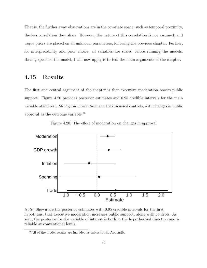
That is, the further away observations are in the covariate space, such as temporal proximity,

the less correlation they share. However, the nature of this correlation is not assumed, and

vague priors are placed on all unknown parameters, following the previous chapter. Further,

for interpretability and prior choice, all variables are scaled before running the models.

Having specified the model, I will now apply it to test the main arguments of the chapter.

4.15 Results

The first and central argument of the chapter is that executive moderation boosts public

support. Figure 4.20 provides posterior estimates and 0.95 credible intervals for the main

variable of interest, Ideological moderation, and the discussed controls, with changes in public

approval as the outcome variable.28

Figure 4.20: The effect of moderation on changes in approval

−1.0 −0.5 0.0 0.5 1.0 1.5 2.0Estimate

Trade

Spending

Inflation

GDP growth

Moderation

Note: Shown are the posterior estimates with 0.95 credible intervals for the firsthypothesis, that executive moderation increases public support, along with controls. Asseen, the posterior for the variable of interest is both in the hypothesized direction and isreliable at conventional levels.

28All of the model results are included as tables in the Appendix.

84

As seen in the figure, GPR provides support for the hypothesized relationship at conven-

tional levels. Specifically, the estimated effect is approximately 0.33. Because all variables

are scaled, this should be interpreted as a one standard deviation shift in the explanatory

variable causes a shift in the outcome variable of 0.33 standard deviations. This translates

to a boost in approval of over 3%. More concrete examples are given below, following the

more nuanced hypothesis test.

As outlined in the previous chapter, the widely applicable information criteria (WAIC)

and the leave-one-out cross validation (LOO) are useful for assessing model fit for GPR using

Hamiltonian MCMC. The WAIC for the full model is −506.4, and the LOO is −645.3. How-

ever, when running the model without including the main explanatory variable, Ideological

moderation, the WAIC and LOO are −674.7 and −901.3, respectively. The differences are

therefore 168.3 for the WAIC and 256.0 for the LOO, with standard errors of 51.6 and 46.4,

both substantial differences, suggesting the model including the main explanatory variable

ought be preferred.

However, I argue that this effect is nuanced and conditional on the expressed extremity of

the president. That is, the more extreme an executive, the greater this effect of moderation

on changes in support. Testing this claim, Figure 4.21 shows the posterior estimates with

0.95 reliable intervals of the variables of interest, Ideological moderation, Extremity, and their

interaction, along with the controls.

While the interaction is in the hypothesized direction, to understand the conditionality of

the effect we have to explore the marginal effects. However, to fully understand the marginal

effect that is not strictly linear, I run the model trained on the observed data and use it to

predict values if Executive moderation was one unit larger than the observed values. I then

take the difference in the outcome, Approval difference, and the predicted outcomes. These

differences along with 0.95 credible intervals are shown in Figure 4.22. Each point is the

predicted difference for a president in a given year. As seen in the figure, the more extreme

85

Figure 4.21: The effect of moderation on changes in approval conditional on extremity

−1.0 −0.5 0.0 0.5 1.0 1.5Estimate

Trade

Spending

Inflation

GDP growth

Moderation x Extremity

Extremity

Moderation

Note: Shown are the posterior estimates with 0.95 credible intervals for the secondhypothesis, that the effect of executive moderation on increased public support isconditional on the extremity of the executive. The estimate for the interaction is in thehypothesized direction and reliable at conventional levels, but Figure 4.22 shows themarginal effect of moderation as extremity increases.

executives enjoy greater shifts in public approval following moderation, while more moderate

executives do not enjoy the same boost in support, and in fact the estimated marginal effect

is negative for the most moderate presidents.

While I do not strictly predict this negative relationship, it is an interesting empiri-

cal trend. Perhaps more moderate executives are viewed as non-committal when moving

in the centrist ideological spectrum, even perceived as switching sides when moderating,

while extremist executives’ shifts towards the center are viewed as necessary moderation

for negotiation. This warrants further investigation that is outside the scope of the current

project. Nevertheless, looking into some of the president’s moves and the associated changes

in approval is a fruitful exercise.

86

Figure 4.22: The predicted point-wise effect of moderation on changes in approval as ex-tremity increases

−1 0 1 2

−2

−1

01

23

Extremity

Pre

dict

ed p

oint

wis

e ef

fect

Note: Shown is the estimated difference in predicted values and actual values whenmoderation increases by one unit, with 0.95 credible intervals. This can be interpreted as apredicted marginal effect. This plot shows predicted values of changes in the outcome atdifferent levels of extremity as moderation increases. Each point represents a president in agiven year.

President Fox of Mexico is the most centrist president in the data. His second speech,

given in 2002, is estimated as the most moderating after his first speech in 2001. His approval

dropped by over 9% points following the speech. His two least moderating speeches, in

which he moved further to the right, are associated with boosts of approval of over 2 and 5%

points. President Garcia of Peru, on the other hand, a relatively extreme leftist, moderated

substantially in 1990 and saw a boost in approval of over 13%, despite significantly negative

GDP growth and overwhelming inflation.

To assess model fit, I compare the model both to the null model including only controls,

and to a model including Ideological moderation and Extremity but not their interaction,

for completeness. Compared to the previously described null model with only controls, the

WAIC differs by 22.9 with a standard error of 6.67, and the LOO differs by 70.8 with a

87

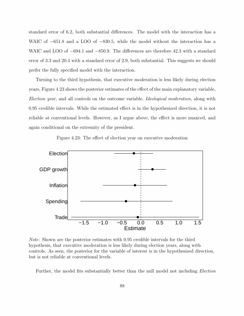
standard error of 6.2, both substantial differences. The model with the interaction has a

WAIC of −651.8 and a LOO of −830.5, while the model without the interaction has a

WAIC and LOO of −694.1 and −850.9. The differences are therefore 42.3 with a standard

error of 3.3 and 20.4 with a standard error of 2.9, both substantial. This suggests we should

prefer the fully specified model with the interaction.

Turning to the third hypothesis, that executive moderation is less likely during election

years, Figure 4.23 shows the posterior estimates of the effect of the main explanatory variable,

Election year, and all controls on the outcome variable, Ideological moderation, along with

0.95 credible intervals. While the estimated effect is in the hypothesized direction, it is not

reliable at conventional levels. However, as I argue above, the effect is more nuanced, and

again conditional on the extremity of the president.

Figure 4.23: The effect of election year on executive moderation

−1.5 −1.0 −0.5 0.0 0.5 1.0 1.5Estimate

Trade

Spending

Inflation

GDP growth

Election

Note: Shown are the posterior estimates with 0.95 credible intervals for the thirdhypothesis, that executive moderation is less likely during election years, along withcontrols. As seen, the posterior for the variable of interest is in the hypothesized direction,but is not reliable at conventional levels.

Further, the model fits substantially better than the null model not including Election

88

year. The model with only the controls has a WAIC and LOO of −3768.9 and −1643.0,

while the model including the explanatory variable has a WAIC and LOO of −1443.6 and

−1643.0, making the differences 2325.3 with a standard error of 580.1 and 1296.1 with a

standard error of 109.6, both large. This implies that while the explanatory variable is not

estimated as having a reliable impact on the outcome variable at conventional levels, the

model including the variable should still be preferred.

Figure 4.24 shows the estimated effect of Election year, Extremity, their interaction, and

all controls on Ideological moderation, along with 0.95 credible intervals. The interaction is

reliable at conventional levels and in the hypothesized direction. Again, however, we need

to investigate the marginal effect of election years on executive moderation as extremity

increases.

Again, the marginal effect is not strictly linear in prediction. I therefore proceed similarly

as before. I train the model on all of the data, and use the model to predict moderation in all

election years if there were not an election. I then take the difference between the observed

level of moderation for these years (N = 38), and the estimated level of moderation had there

not been an election. Figure 4.25 shows these predicted differences as extremity increases.

I repeat this process for non-election years (N = 70), predicting the differences if there

were an election. These predictive differences are shown in Figure 4.26. At higher levels of

extremity, executives are indeed less likely to moderate during election years. Very moderate

presidents, on the other hand, are estimated to moderate more during election years, likely

attempting to target the median voter and increase overall support, as opposed to targeting

the loyal, generally extreme supporters presidents and parties at far ends of the ideological

spectrum tend to target.

Again, to assess model fit, I employ WAIC and LOO. The values are, respectively,

−1303.8 and −1411.0. Compared to the null model only including controls, this leads to the

substantial differences of 2465.0 with a standard error of 646.4 and 1528.1 with a standard

89

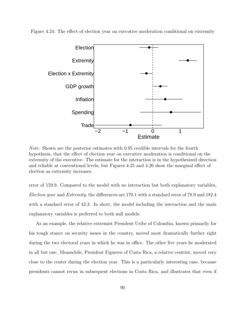
Figure 4.24: The effect of election year on executive moderation conditional on extremity

−2 −1 0 1Estimate

Trade

Spending

Inflation

GDP growth

Election x Extremity

Extremity

Election

Note: Shown are the posterior estimates with 0.95 credible intervals for the fourthhypothesis, that the effect of election year on executive moderation is conditional on theextremity of the executive. The estimate for the interaction is in the hypothesized directionand reliable at conventional levels, but Figures 4.25 and 4.26 show the marginal effect ofelection as extremity increases.

error of 159.9. Compared to the model with no interaction but both explanatory variables,

Election year and Extremity, the differences are 170.1 with a standard error of 78.9 and 182.4

with a standard error of 42.3. In short, the model including the interaction and the main

explanatory variables is preferred to both null models.

As an example, the relative extremist President Uribe of Colombia, known primarily for

his tough stance on security issues in the country, moved most dramatically further right

during the two electoral years in which he was in office. The other five years he moderated

in all but one. Meanwhile, President Figueres of Costa Rica, a relative centrist, moved very

close to the center during the election year. This is a particularly interesting case, because

presidents cannot rerun in subsequent elections in Costa Rica, and illustrates that even if

90

Figure 4.25: The predicted point-wise effect of election year in election years on moderationas extremity increases

−1.5 −1.0 −0.5 0.0 0.5 1.0 1.5

−6

−4

−2

02

Extremity

Pre

dict

ed p

oint

wis

e ef

fect

Note: Shown is the difference between moderation in an election year and the predictedmoderation in a non-election year as extremity increases, with 0.95 reliable intervals. Thereare 38 election years, and each point represents the difference in actual moderation in theseyears and the predicted level of moderation, had there not been an election. Moderatepresidents are estimated to moderate more in election years, and extreme executives areestimated to moderate less in election years.

the president is not running, there is incentive for party success.

4.15.1 Comparison to Alternative Modeling Choices

While analyses of these data suffer the common problems in TSCS applications, and I argue

that the approach taken in the previous chapter is the best method of analyzing these data,

comparison to more conventional modeling strategies may provide some completeness of the

results. Across all four hypotheses, I compare GPR to a two-way fixed-effects regression

using robust clustered standard errors (RCSE), panel corrected standard errors (PCSE), a

lagged dependent variable model (LDV), and a two-way random effects model (RE), following

Chapter 3.

91

Figure 4.26: The predicted point-wise effect of election year in non-election years on moder-ation as extremity increases

−1 0 1 2−4

−2

02

4

Extremity

Pre

dict

ed p

oint

wis

e ef

fect

Note: Shown is the difference between the predicted moderation in an election year andthe observed moderation in a non-election year as extremity increases, with 0.95 reliableintervals. There are 70 non-election years, and each point represents the difference in thepredicted level of moderation if there had been an election, and the actual observed level ofmoderation in these non-election years. Moderate presidents are estimated to moderatemore in election years, and extreme executives are estimated to moderate less in electionyears.

I argue that all of these models are over-specified, and the degrees of freedom lost from

two-way effects models is not warranted (Greene 2003, p. 364). In addition, these mod-

els can accentuate problems of multicollinearity among regressors (Baltagi 2008, p. 35).

Nevertheless, due to the novelty of the chosen modeling strategy, a comparison is useful.

For the first hypothesis, that Executive moderation positively affects Approval difference,

the results are not reliable at conventional levels for any modeling strategy but the random

effects model. RCSE, PCSE, and LDV all produce positive estimates, but are only reliable

at the 0.90 credible level. Specifically, RCSE estimates the effect is 0.19 with a standard

92

error of 0.11. PCSE29 estimates the effect to be 0.29 with a standard error of 0.15. RE

estimates the effect to be 0.19 (SE = 0.06). Finally, LDV estimates an effect of 0.16 (SE

= 0.09). These estimates with 0.95 and 0.90 reliable intervals are shown in Figure 4.27.

Figure 4.27: The effect of executive moderation on changes in public approval, model com-parison

−0.1 0.0 0.1 0.2 0.3 0.4 0.5Estimate

RE

LDV

PCSE

RCSE

GPR

Note: Shown are estimates with 0.95 and 0.90 reliable intervals for the effect of executivemoderation on changes in public approval using the most common modeling strategies forTSCS data, along with the estimated effect using GPR.

The second hypothesis is that this effect is conditional on Extremity. The interaction

between Extremity and Executive moderation is reliable at conventional levels for RCSE

and PCSE, but not RE or LDV. To be more precise, the estimate for RCSE is 0.16 with

a standard error of 0.07. PCSE estimates an effect of 0.25 (SE = 0.11). The RE estimate

is 0.10 (SE = 0.06), reliable at the 0.90 level but not 0.95. The LDV model estimates an

effect of 0.11 (SE = 0.08). These estimates with 0.95 and 0.90 reliable intervals are shown

in Figure 4.28.

GPR does not provide conventionally reliable support for the third hypothesis, that

29In order to identify the PCSE model, presidents and years with only one observation need to be dropped,so the estimates are not identical to RCSE.

93

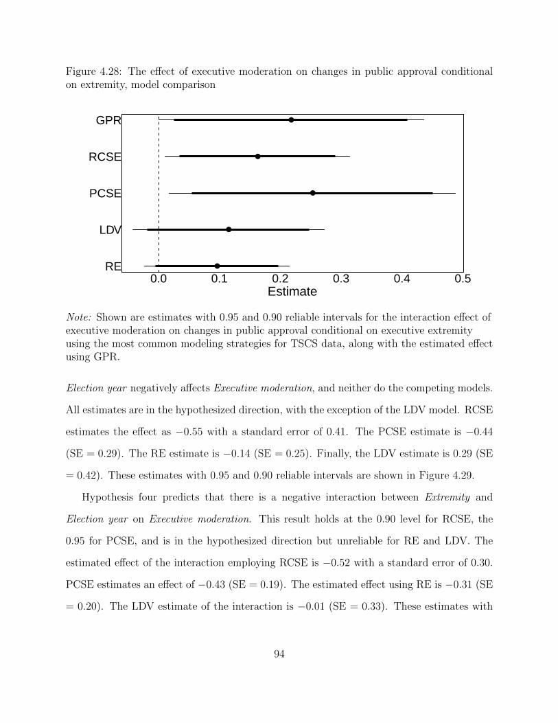
Figure 4.28: The effect of executive moderation on changes in public approval conditionalon extremity, model comparison

0.0 0.1 0.2 0.3 0.4 0.5Estimate

RE

LDV

PCSE

RCSE

GPR

Note: Shown are estimates with 0.95 and 0.90 reliable intervals for the interaction effect ofexecutive moderation on changes in public approval conditional on executive extremityusing the most common modeling strategies for TSCS data, along with the estimated effectusing GPR.

Election year negatively affects Executive moderation, and neither do the competing models.

All estimates are in the hypothesized direction, with the exception of the LDV model. RCSE

estimates the effect as −0.55 with a standard error of 0.41. The PCSE estimate is −0.44

(SE = 0.29). The RE estimate is −0.14 (SE = 0.25). Finally, the LDV estimate is 0.29 (SE

= 0.42). These estimates with 0.95 and 0.90 reliable intervals are shown in Figure 4.29.

Hypothesis four predicts that there is a negative interaction between Extremity and

Election year on Executive moderation. This result holds at the 0.90 level for RCSE, the

0.95 for PCSE, and is in the hypothesized direction but unreliable for RE and LDV. The

estimated effect of the interaction employing RCSE is −0.52 with a standard error of 0.30.

PCSE estimates an effect of −0.43 (SE = 0.19). The estimated effect using RE is −0.31 (SE

= 0.20). The LDV estimate of the interaction is −0.01 (SE = 0.33). These estimates with

94

Figure 4.29: The effect of election year on executive moderation, model comparison

−1.0 −0.5 0.0 0.5 1.0Estimate

RE

LDV

PCSE

RCSE

GPR

Note: Shown are estimates with 0.95 and 0.90 reliable intervals for the effect of electionyear on executive moderation using the most common modeling strategies for TSCS data,along with the estimated effect using GPR.

0.95 and 0.90 reliable intervals are shown in Figure 4.30.

This subsection highlights that modeling choice can sometimes make a difference on our

substantive conclusions. However, the modeling strategies employed here are largely conso-

nant with GPR. Where there is disagreement, because GPR makes fewer assumptions about

the underlying data-generating process, and the assumptions made are relatively realistic,

we should consider GPR as the best modeling strategy. While other methods produce mixed

results with regards to the hypotheses, these results are based on models with problematic

issues as discussed in the previous chapter (see also Esarey and Menger 2017). Further, as I

already mention, the degrees of freedom lost to these two-way effect models is not justified,

and severely diminishes the explanatory power of our variables of interest on the outcome.

95

Figure 4.30: The effect of election year on executive moderation conditional on extremity,model comparison

−1.0 −0.5 0.0 0.5Estimate

RE

LDV

PCSE

RCSE

GPR

Note: Shown are estimates with 0.95 and 0.90 reliable intervals for the interaction effect ofelection year on executive moderation conditional on executive extremity using the mostcommon modeling strategies for TSCS data, along with the estimated effect using GPR.

4.16 Conclusion

This chapter argues that presidents across Latin America enjoy a boost of public support

following moderation of their expressed ideological points. These benefits are heterogeneous,

however, and the more extreme an executive the greater the increased support following

shifts. Further, executives, particularly extreme executives, are less willing to moderate

during election years in order to target their core voters.

To test these arguments, I apply Gaussian process regression for time-series cross-sectional

analyses. The data consist of yearly ideological points as estimated from the constitutionally

imposed annual presidential addresses, along with yearly public approval data from repre-

sentative surveys. The results are largely in line with expectations, and begin to fill the

gap in the literature on the effect of executive ideological movement on public opinion, and

therefore the incentives for executives to shift.

96

However, there are still open questions for future research. For example, empirically,

more moderate presidents seem to be publicly damaged following ideological moderation.

This could be due to perceptions of switching sides, and may even be linked to the nuances

of coalition building and cross-assembly support. There is also the question of endogeneity.

Less popular presidents may change their professed ideology in order to become more popular.

Further, more moderate executives do not seem to move to the extremes during election

years, but instead move further towards the center. While this chapter argues this is due to

different electoral dynamics of support for these executives and their parties, there is no test

of the underlying causal mechanism for this argument.

Finally, while suggestive of which presidents benefit from moderation and why we see

heterogeneity of presidential willingness to moderate, this chapter does not explore the true

ideal points of executives, only their professed ideal points, and can therefore not make

strong claims about the incentives presidents face for moderation. Further work in this area

would be fruitful. To conclude, this project starts to help us better understand the causes

and consequences of presidential movement, but also opens the door for more work in this

area.

97

Concluding Remarks

The three main chapters of this dissertation argue that the modeling assumption of condi-

tional independence is often violated, and this violation is often ignored in political science

research. Ignoring this fundamental principle can lead to biased estimates, inefficient estima-

tors, and incorrect substantive conclusions. We also lose some of the nuance of the theoretical

understanding of political science by not addressing this problem. The dissertation in part

is therefore a claim that the discipline needs to be more careful about understanding the

true data-generating process that leads to our observations, and needs to model the data in

a more thoughtful manner that represents the underlying relationships between variables in

which we have interest.

I begin to address some of the more common analyses we encounter in political science,

particularly comparative political science, by developing two models. The second chapter

develops a zero-inflated multivariate ordered probit to handle ordered, multivariate outcomes

that may share a relationship in the underlying dynamics that generate the observations.

I apply the model to party campaign dynamics, but the model can be utilized for many

questions in comparative political science. Ordered outcomes are very common, and in

comparative politics there is often a reason to doubt the assumption that (1) the outcomes

do not share commonalities in the underlying data-generating process, and (2) every actor

or unit of observation responds to observables in the same manner. The chapter therefore

provides a very useful model, and suggests how to carefully consider the underlying nature

98

of the models chosen for analyzing data commonly encountered in the discipline.

The third chapter uniquely parameterizes Gaussian process regression (GPR) for applica-

tions to time-series cross-sectional (TSCS) data. While not a new model, it is underutilized

in political science and this chapter not only helps introduce the model to the discipline but

demonstrates how it can be changed for our purposes as social scientists. Though specific

to TSCS data in this chapter, of which analyses commonly suffer problems that GPR helps

alleviate, many other types of analyses can benefit from considering models of this class.

Both of these chapters also discuss and show through example how these models can be

applied in the discipline.

Further, all three chapters aid in our understanding of comparative politics in Latin

America and politics more generally. The second chapter, using Mexico as a case study,

shows that the choices for presidential campaigns to visit a municipality or hold a rally

are related to other campaigns’ decisions. Further, the strategic calculi for municipal-level

behavior varies from party to party. Campaigns do not respond to the same variables in the

same way. This is a novel finding that likely generalizes to other cases, and would be missed

with traditional analysis techniques.

The third chapter demonstrates that inflation in Latin America leads to decreased anti-

American sentiment in the region. Latin American citizens view the United States as a source

of economic well-being. When the economy, specifically the citizens’ purchasing power, a

very tangible economic indicator, is not doing well, they want to increase relations with

the United States and see the U.S. as a way out of their economic hardship. This finding

helps us better understand the international perceptions of the United States and in which

circustances these perceptions may change. This chapter also re-analyzes, with stronger

results, the effect of rocket threat on the right vote in Israel. Voters who are within range

of Palestinian rockets are substantially more likely to vote for parties on the right. This is

in line with previous research, but the magnitude of the relationship is much stronger than

99

previously thought.

The fourth chapter generates and tests more in-depth hypotheses, specifically regard-

ing Latin American presidential position-taking and the effect this has on executive public

approval, and therefore the incentives for executive ideological movement. I argue that presi-

dential moderation in their professed ideology increases overall public support. This support

is beneficial to the executive both in its own right and because it increases legislative bar-

gaining power. However, extreme executives enjoy greater benefit from moderation. This

moderation comes at a cost, particularly for relatively extreme executives, by decreasing the

enthusiasm of their core supporters. Therefore, in order to turn out the vote and appeal to

their core supporters and activists, this moderation is less likely during election years, and

extreme executives will shift their professed ideology back to the extremes. This relation-

ship between executive movement and public perception has been largely ignored in Latin

America, and this chapter begins to address this oversight.

The dissertation contributes both methodologically and theoretically to political science,

particularly comparative political science in Latin America. However, it also opens the

door for more research, again both methodologically and theoretically. Before discussing the

drawbacks of the dissertation and directions for future work, I will outline my plans for the

progression of the dissertation.

5.17 Related Future Work

This dissertation opens the door for much future work. The second chapter develops a zero-

inflated multivariate ordered probit, and applies it to an interesting substantive question.

However, there are two drawbacks. The first is that the model is computationally very

expensive. I intend to recode the model in Stan in order to increase the speed with which

the model is estimated. I then plan to write an easy to use R package that will allow much

100

easier estimation with the model for the end user. This will be published on CRAN shortly

thereafter.

The second drawback of the ZIMVOP model is that consumers may not know how to

apply it to their own substantive questions. I plan, as part of the package development,

to write open-source vignettes that apply the model to a few more substantive questions

using the developed package. While work on this model will not result in peer-reviewed

publications, I strongly believe it will help increase the model’s exposure and future use to

researchers in the field.

The third chapter introduces Gaussian process regression (GPR) as a solution to time-

series cross-sectional analyses. However, the applications are nearly endless. We have strong

reason to doubt our modeling assumption of conditional independence in many situations,

and I plan to capitalize on the model’s relaxation of this assumption for many more applica-

tions. For example, while Monogan and Gill (2016) make great strides introducing Bayesian

kriging to spatial applications, very little attention has been paid to this work in compar-

ative politics. Further, the implications this work can have on spill-over effects, spatial

correlations, and any question regarding geographic units have not been fully exploited.

Computer scientists and statisticians have also made numerous developments to the Gaus-

sian process of which political scientists are seemingly unaware. There are almost countless

projects that I envision introducing these strides to the political science literature. As an

example, Roman Garnett, Jacob M. Montgomery, and I are working to improve sentiment

analysis of political text using Gaussian process machine learning algorithms. I also have

several ideas for future sole- and / or co-authored work further developing and introducing

this class of models to the discipline.

Finally, the fourth chapter, while introducing and validating novel hypotheses, also leaves

unanswered questions that I plan to continue investigating. For example, developing a more

granular measure of professed ideal points for presidents to test richer hypotheses would be

101

fruitful. Executives are communicating to the public in many ways other than the annual

addresses. Unfortunately, this will require a major data-gathering exercise. Fortunately,

with the funding and research assistance I will have in the coming years, I should be able to

make great advances towards reaching this goal.

The fourth chapter also does not adequately test the effect of professed moderation or

movements to the extreme by centrist executives on public perception. I believe that a

survey experiment is the best avenue to approach this. It can help us better understand why

moderation by centrist executives seems to harm the executive’s public approval.

To conclude, this dissertation solves many methodological and theoretical problems in

political science. It also, however, will continue developing novel work in methodology,

comparative politics, and Latin American politics.

102

References

Abranches, Sergio. 1988. “Presidencialismo de coalizao: o dilema institucional brasileiro”.

Dados 31 (1): 5–38.

Albert, James H, and Siddhartha Chib. 1993. “Bayesian analysis of binary and polychoto-

mous response data”. Journal of the American Statistical Association 88 (422): 669–679.

Aleman, Eduardo, and George Tsebelis. 2011. “Political parties and government coalitions

in the Americas”. Journal of Politics in Latin America 3 (1): 3–28.

— . 2005. “The origins of presidential conditional agenda-setting power in Latin America”.

Latin American Research Review 40 (2): 3–26.

Ames, Barry. 2001. “The deadlock of democracy in Brazil: interests, identities, and institu-

tions in comparative politics”. Ann Arbor: University of Michigan Press.

Amorim Neto, Octavio. 2002. “Presidential Cabinets and Legislative Cohesion in Brazil”.

Legislative Politics in Latin America: 48–78.

— . 2006. “The presidential calculus: Executive policy making and cabinet formation in the

Americas”. Comparative Political Studies 39 (4): 415–440.

Andrews, Donald W. K. 1991. “Heteroskedasticity and Autocorrelation Consistent Covari-

ance Matrix Estimation”. Econometrica 59 (3): 817–858. issn: 00129682, 14680262. http:

//www.jstor.org/stable/2938229.

103

Arel-Bundock, Vincent. 2013. WDI: World Development Indicators (World Bank). R package

version 2.4. https://CRAN.R-project.org/package=WDI.

Arnold, Christian, David Doyle, and Nina Wiesehomeier. 2017. “Presidents, Policy Compro-

mise, and Legislative Success”. The Journal of Politics 79 (2): 380–395.

Bagozzi, Benjamin E, and Kathleen Marchetti. 2014. “Distinguishing occasional abstention

from routine indifference in models of vote choice”. Political Science Research and Meth-

ods.

Bagozzi, Benjamin E, et al. 2015. “Modeling two types of peace: The zero-inflated ordered

probit (ZiOP) model in conflict research”. Journal of Conflict Resolution 59 (4): 728–752.

Baker, Andy. 2003. “Why is trade reform so popular in Latin America?: A consumption-

based theory of trade policy preferences”. World Politics 55 (3): 423–455.

Baker, Andy, and David Cupery. 2013. “Anti-Americanism in Latin America: Economic

exchange, foreign policy legacies, and mass attitudes toward the colossus of the North”.

Latin American Research Review 48 (2): 106–130.

Baltagi, Badi. 2008. Econometric analysis of panel data. John Wiley & Sons.

Barnard, John, Robert McCulloch, and Xiao-Li Meng. 2000. “Modeling covariance matrices

in terms of standard deviations and correlations, with application to shrinkage”. Statistica

Sinica: 1281–1311.

Bas, Muhammet Ali, Curtis S Signorino, and Robert W Walker. 2008. “Statistical backwards

induction: A simple method for estimating recursive strategic models”. Political Analysis

16 (1): 21–40.

Beck, Nathaniel. 1985. “Estimating Dynamic Models is Not Merely a Matter of Technique”.

Political Methodology 11 (1/2): 71–89. issn: 01622021. http://www.jstor.org/stable/

41289329.

104

Beck, Nathaniel, and Jonathan N Katz. 1995. “What to do (and not to do) with time-series

cross-section data”. American political science review 89 (03): 634–647.

Borel, Emile. 1921. “La theorie du jeu et les equations integrales a noyau symetrique”.

Comptes Rendus de l’Academie des Sciences 173 (58): 1304–1308.

Calvo, Ernesto. 2007. “The responsive legislature: Public opinion and law making in a highly

disciplined legislature”. British Journal of Political Science 37 (2): 263–280.

Cameron, A Colin, Jonah B Gelbach, and Douglas L Miller. 2008. “Bootstrap-based im-

provements for inference with clustered errors”. The Review of Economics and Statistics

90 (3): 414–427.

— . 2011. “Robust inference with multiway clustering”. Journal of Business & Economic

Statistics 29 (2): 238–249.

Cameron, A Colin, and Douglas L Miller. 2015. “A practitioner’s guide to cluster-robust

inference”. Journal of Human Resources 50 (2): 317–372.

— . 2012. “Robust Inference with Dyadic Data: with Applications to Country-pair Interna-

tional Trade”. University of California-Davis. Unpublished.

Cameron, A Colin, and Pravin K Trivedi. 2005. Microeconometrics: Methods and applica-

tions. Cambridge university press.

Campello, Daniela. 2014. “The politics of financial booms and crises: Evidence from Latin

America”. Comparative Political Studies 47 (2): 260–286.

— . 2015. The Politics of Market Discipline in Latin America. Cambridge University Press.

Carlin, Ryan E, Gregory J Love, and Cecilia Martınez-Gallardo. 2015. “Cushioning the fall:

Scandals, economic conditions, and executive approval”. Political Behavior 37 (1): 109–

130.

105

Carlin, Ryan E., et al. 2016. Executive Approval Database. www.executiveapproval.org.

Version 1.0.

Carpenter, Bob, et al. 2016. “Stan: A probabilistic programming language”. In press, Journal

of Statistical Software.

Carson, Jamie L, and Jason M Roberts. 2005. “Strategic politicians and US House elections,

1874–1914”. Journal of Politics 67 (2): 474–496.

Cason, Jeffrey. 2002. “Electoral reform, institutional change, and party adaptation in Uruguay”.

Latin American Politics and Society 44 (3): 89–109.

Chasquetti, Daniel. 2001. “Elecciones presidenciales mayoritarias en America Latina”.

Cheibub, Jose Antonio. 2007. Presidentialism, parliamentarism, and democracy. Cambridge

University Press.

Cheibub, Jose Antonio, Adam Przeworski, and Sebastian M Saiegh. 2004. “Government

coalitions and legislative success under presidentialism and parliamentarism”. British

Journal of Political Science 34 (4): 565–587.

Claude, Luis Lezcano. 2000. “El control de constitucionalidad sobre actos de los poderes

legislativo y ejecutivo en el Paraguay”. Anuario iberoamericano de justicia constitucional,

no. 4: 221–242.

Colomer, Josep M, and Gabriel L Negretto. 2005. “Can presidentialism work like parliamen-

tarism?” Government and Opposition 40 (1): 60–89.

Cox, Gary W. 1990. “Centripetal & Centrifugal Incentives in Electoral Systems”. American

Journal of Political Science 34:903–935.

Cox, Gary W., and Matthew D. McCubbins. 2005. Setting the Agenda: Responsible Party

Government in the US House of Representatives. New York: Cambridge University Press.

106

Cox, Gary W, and Scott Morgenstern. 2001. “Latin America’s reactive assemblies and proac-

tive presidents”. Comparative Politics : 171–189.

Dunne, John Paul, and Nan Tian. “The determinants of civil war and excess zeros”. Working

Paper.

Esarey, Justin, and Jacob Jaffe. 2017. “A Direct Test for Consistency of Random Effects

Models that Outperforms the Hausman Test”.

Esarey, Justin, and Andrew Menger. 2017. “Practical and Effective Approaches to Dealing

with Clustered Data”. Department of Political Science, Rice University, Unpublished

Manuscript.

Florensa, Luis Marcelo, Laura Marquez-Ramos, and Marıa Luisa Recalde. 2015. “The effect

of economic integration and institutional quality of trade agreements on trade margins:

evidence for Latin America”. Review of World Economics 151 (2): 329–351.

Fonseca, Carlos da. 2008. “O Governo George W. Bush e o relacionamento EUA-America

Latina”. Relacoes Internacionais (R: I), no. 19: 147–158.

Garg, Sahil, Amarjeet Singh, and Fabio Ramos. 2012. “Learning non-stationary space-time

models for environmental monitoring”. In Proceedings of the AAAI Conference on Arti-

ficial Intelligence, 25:45. 35.

Getmansky, Anna, and Thomas Zeitzoff. 2014. “Terrorism and Voting: The Effect of Rocket

Threat on Voting in Israeli Elections”. American Political Science Review 108 (3): 588–

604. doi:10.1017/S0003055414000288.

Gibson, NP, et al. 2012. “A Gaussian process framework for modelling instrumental system-

atics: application to transmission spectroscopy”. Monthly notices of the royal astronomical

society 419 (3): 2683–2694.

107

Gramacy, Robert B. 2005. “Bayesian treed Gaussian process models”. PhD thesis, UNIVER-

SITY OF CALIFORNIA SANTA CRUZ.

Gramacy, Robert B, and Herbert K H Lee. 2008. “Bayesian treed Gaussian process models

with an application to computer modeling”. Journal of the American Statistical Associ-

ation 103 (483): 1119–1130.

Granger, Clive WJ, and Paul Newbold. 1974. “Spurious regressions in econometrics”. Journal

of Econometrics 2 (2): 111–120.

Greene, William H. 2003. Econometric analysis. Pearson Education India.

Gurmu, Shiferaw, and Getachew A Dagne. 2012. “Bayesian approach to zero-inflated bi-

variate ordered probit regression model, with an application to tobacco use”. Journal of

Probability and Statistics 2012.

Hainmueller, Jens, and Chad Hazlett. 2013. “Kernel regularized least squares: Reducing mis-

specification bias with a flexible and interpretable machine learning approach”. Political

Analysis 22 (2): 143–168.

Harris, Mark N, and Xueyan Zhao. 2007. “A zero-inflated ordered probit model, with an

application to modelling tobacco consumption”. Journal of Econometrics 141 (2): 1073–

1099.

Hausman, Jerry A. 1978. “Specification tests in econometrics”. Econometrica: Journal of the

Econometric Society : 1251–1271.

Hawkins, Douglas M. 2004. “The problem of overfitting”. Journal of chemical information

and computer sciences 44 (1): 1–12.

Huang, Biwei, Kun Zhang, and Bernhard Scholkopf. 2015. “Identification of Time-Dependent

Causal Model: A Gaussian Process Treatment.” In IJCAI, 3561–3568.

108

Ibragimov, Rustam, and Ulrich K Muller. 2010. “t-Statistic based correlation and hetero-

geneity robust inference”. Journal of Business & Economic Statistics 28 (4): 453–468.

Ionides, Edward L. 2008. “Truncated importance sampling”. Journal of Computational and

Graphical Statistics 17 (2): 295–311.

Johnson, Gregg B, and Brian F Crisp. 2003. “Mandates, powers, and policies”. American

Journal of Political Science 47 (1): 128–142.

Kadel, Rajendra. 2013. “A latent mixture approach to modeling zero-inflated bivariate or-

dinal data”. PhD thesis, University of South Florida.

Kaplan, Stephen B. 2013. Globalization and austerity politics in Latin America. Cambridge

University Press.

Keele, Luke, and Nathan J Kelly. 2005. “Dynamic models for dynamic theories: The ins and

outs of lagged dependent variables”. Political analysis 14 (2): 186–205.

Kiewit, Rodrik, and Matthew McCubbins. 1991. “The Logic of Delegation Chicago”. IL:

University of Chicago.

King, Gary. 1989. “A seemingly unrelated Poisson regression model”. Sociological Methods

& Research 17 (3): 235–255.

King, Gary, and Margaret E Roberts. 2015. “How robust standard errors expose method-

ological problems they do not fix, and what to do about it”. Political Analysis 23 (2):

159–179.

King, Gary, and Langche Zeng. 2001a. “Explaining rare events in international relations”.

International Organization 55 (03): 693–715.

— . 2001b. “Logistic regression in rare events data”. Political Analysis 9 (2): 137–163.

109

Kirk, Paul DW, and Michael PH Stumpf. 2009. “Gaussian process regression bootstrapping:

exploring the effects of uncertainty in time course data”. Bioinformatics 25 (10): 1300–

1306.

Lambert, Peter. 2000. “A decade of electoral democracy: continuity, change and crisis in

Paraguay”. Bulletin of Latin American Research 19 (3): 379–396.

Langston, Joy, and Guillermo Rosas. 2016. “Presidential campaigns under single-district

plurality: Visits, rallies, and the calculus of electoral mobilzation in Mexico”. Submitted.

Laslier, Jean-Francois, and Nathalie Picard. 2002. “Distributive politics and electoral com-

petition”. Journal of Economic Theory 103 (1): 106–130.

Liang, Kung-Yee, and Scott L Zeger. 1986. “Longitudinal data analysis using generalized

linear models”. Biometrika 73 (1): 13–22.

Linz, Juan J. 1990. “The perils of presidentialism”. Journal of Democracy 1 (1): 51–69.

Lupu, Noam. 2016. Party brands in crisis: partisanship, brand dilution, and the breakdown

of political parties in Latin America. Cambridge University Press.

Maeda, Ko. 2010. “Two modes of democratic breakdown: A competing risks analysis of

democratic durability”. The Journal of Politics 72 (4): 1129–1143.

Mainwaring, Scott. 1993. “Presidentialism, multipartism, and democracy: The difficult com-

bination”. Comparative Political Studies 26 (2): 198–228.

Martinez-Gallardo, Cecilia. 2011. “Designing cabinets: presidential politics and cabinet in-

stability in Latin America”. University of Notre Dame, Kellogg Institute Working Paper

(375).

Milner, Helen V, and Keiko Kubota. 2005. “Why the move to free trade? Democracy and

trade policy in the developing countries”. International Organization 59 (1): 107–143.

110

Monogan, James E. 2015. Political Analysis Using R. Switzerland: Springer Internation Pub-

lishing.

Monogan, James E, and Jeff Gill. 2016. “Measuring State and District Ideology with Spatial

Realignment”. Political Science Research and Methods 4 (01): 97–121.

Mundlak, Yair. 1978. “On the pooling of time series and cross section data”. Econometrica:

Journal of the Econometric Society : 69–85.

Myerson, Roger B. 1993. “Incentives to cultivate favored minorities under alternative elec-

toral systems.” American Political Science Review 87 (04): 856–869.

Negretto, Gabriel L. 2006. “Minority presidents and democratic performance in Latin Amer-

ica”. Latin American Politics and Society 48 (3): 63–92.

Newey, Whitney K. 1985. “Maximum likelihood specification testing and conditional moment

tests”. Econometrica: Journal of the Econometric Society : 1047–1070.

Newey, Whitney K., and Kenneth D. West. 1987. “A Simple, Positive Semi-Definite, Het-

eroskedasticity and Autocorrelation Consistent Covariance Matrix”. Econometrica 55 (3):

703–708. issn: 00129682, 14680262. http://www.jstor.org/stable/1913610.

Nieman, Mark David. 2015. “Statistical Analysis of Strategic Interaction with Unobserved

Player Actions: Introducing a Strategic Probit with Partial Observability”. Political Anal-

ysis. doi:10.1093/pan/mpv003. eprint: http://pan.oxfordjournals.org/content/

early/2015/03/22/pan.mpv003.full.pdf+html.

Pang, Xun. 2014. “Varying responses to common shocks and complex cross-sectional de-

pendence: dynamic multilevel modeling with multifactor error structures for time-series

cross-sectional data”. Political Analysis 22 (4): 464–496.

Petras, James, and Henry Veltmeyer. 2016. What’s left in Latin America?: Regime change

in new times. Routledge.

111

Proksch, Sven-Oliver, and Jonathan B Slapin. 2008. “WORDFISH: Scaling software for

estimating political positions from texts”. Version 1:323–344.

Qian, P, Y Zhou, and C Rudin. 2011. “Using Gaussian processes to monitor diabetes de-

velopment”. In Proceedings of the 6th INFORMS Workshop on Data Mining and Health

Informatics (DM-HI 2011) P. Qian, Y. Zhou, C. Rudin, eds.

Raile, Eric D, Carlos Pereira, and Timothy J Power. 2011. “The executive toolbox: Building

legislative support in a multiparty presidential regime”. Political Research Quarterly 64

(2): 323–334.

Rasmussen, Carl Edward, and Christopher KI Williams. 2006. Gaussian processes for ma-

chine learning. Vol. 1. MIT press Cambridge.

Romero, Luis Alberto. 2013. A History of Argentina in the Twentieth Century: Updated and

Revised Edition. Penn State Press.

Saiegh, Sebastian M. 2009. “Political prowess or “Lady Luck”? Evaluating chief executives’

legislative success rates”. The Journal of Politics 71 (4): 1342–1356.

Saiegh, Sebastian M. 2015. “Using joint scaling methods to study ideology and representa-

tion: Evidence from Latin America”. Political Analysis 23 (3): 363–384.

Samuels, David. 2008a. “Brazilian Democracy under Lula and the PT”. Constructing Demo-

cratic Governance in Latin America: 15–32.

— . 2008b. “Political ambition, candidate recruitment, and legislative politics in Brazil”.

Pathways to Power. Political Recruitment and Candidate Selection in Latin America.

Pennsylvania, The Pennsylvania State University Press : 76–91.

Samuels, David J, and Matthew S Shugart. 2010. Presidents, parties, and prime ministers:

How the separation of powers affects party organization and behavior. Cambridge Univer-

sity Press.

112

Signorino, Curtis. 2002. “Strategy and selection in international relations”. International

Interactions 28 (1): 93–115.

Signorino, Curtis S. 2003. “Structure and uncertainty in discrete choice models”. Political

Analysis 11 (4): 316–344.

Stepan, Alfred, and Cindy Skach. 1993. “Constitutional frameworks and democratic consol-

idation: Parliamentarianism versus presidentialism”. World Politics 46 (1): 1–22.

Stokes, Susan C. 2001. Mandates and democracy: Neoliberalism by surprise in Latin America.

Cambridge University Press.

Strom, Kaare. 1990. “A behavioral theory of competitive political parties”. American Journal

of Political Science: 565–598.

Tauchen, George. 1985. “Diagnostic testing and evaluation of maximum likelihood models”.

Journal of Econometrics 30 (1-2): 415–443.

Vehtari, Aki, Andrew Gelman, and Jonah Gabry. 2016a. loo: Efficient leave-one-out cross-

validation and WAIC for Bayesian models. R package version 1.0.0. https://github.

com/stan-dev/loo.

— . 2016b. “Practical Bayesian model evaluation using leave-one-out cross-validation and

WAIC”. Statistics and Computing.

Watanabe, Sumio. 2010. “Asymptotic equivalence of Bayes cross validation and widely ap-

plicable information criterion in singular learning theory”. Journal of Machine Learning

Research 11 (Dec): 3571–3594.

Weiss, Arriaga, Vıctor A Suarez Arguello, Ana Rosa Suarez Arguello, et al. 1995. “Estados

Unidos desde America Latinasociedad, polıtica y cultura”. In Encuentro de Latinoamer-

icanos Dedicados al Estudio de Estados Unidos. 2o. 1992. Mexico, DF. 330.973 E5.

113

White, Halbert. 1980. “A heteroskedasticity-consistent covariance matrix estimator and a

direct test for heteroskedasticity”. Econometrica: Journal of the Econometric Society :

817–838.

— . 1982. “Maximum likelihood estimation of misspecified models”. Econometrica: Journal

of the Econometric Society : 1–25.

Wiesehomeier, Nina, and Kenneth Benoit. 2009. “Presidents, parties, and policy competi-

tion”. The Journal of Politics 71 (4): 1435–1447.

Zellner, Arnold. 1962. “An efficient method of estimating seemingly unrelated regressions

and tests for aggregation bias”. Journal of the American Statistical Association 57 (298):

348–368.

Zellner, Arnold, and David S Huang. 1962. “Further properties of efficient estimators for

seemingly unrelated regression equations”. International Economic Review 3 (3): 300–

313.

114

Appendix

7.18 Modeling Related Processes with an Excess of Ze-

ros Supplementary Information

7.18.1 ZIMVOP JAGS Model

The JAGS model follows the chapter’s specification, and is quite general. It can handle any

number of predictors, any number of dimensions, and any number of cut-offs within the

different dimensions. It assumes that there is some observation-level data that can predict

participation, and once participation is attained, it predicts the level of participation on

all d dimensions. The estimated variance-covariance matrix can be used to determine the

correlations between dimensions.

model

#y is a matrix of outcomes of dimension NxD

#N is the number of observations

#D is the number of dimensions

#Z is the matrix of first-stage predictors of dimension NxK

#K is the number of first-stage predictors, including an intercept

#X is an array of predictors for the second stage

#n.cut is a scalar, the number of cut points

#c is a vector, the second cut point

#R is the inverse-Wishart prior matrix

115

for(i in 1:N)

#if outcomes have different number of levels, change n.cut to a vector

#first stage

S[i] <- max(min(S.star[i],1),0)

probit(S.star[i]) <- s.star[i] #participation regime probability

s.star[i] <- inprod(Z[i,], gamma[1:K])

#second stage

for(d in 1:D)

Xnew[d,i] <- inprod(X[i,,d], beta[1:J,d])

y.star[i, 1:D] ~ dmnorm(Xnew[,i], invW[,])

for(d in 1:D)

for (i.cut in 1:n.cut)

probit(Q[i,i.cut,d]) <- tau.unsorted[i.cut, d] - y.star[i,d]

for(d in 1:D)

p[i,d,1] <- (1-S[i]) + S[i]*max(min(Q[i,1,d],1),0)

for(i.cut in 2:n.cut)

p[i,d,i.cut] <- S[i]*(max(min(Q[i,i.cut,d],1),0) - max(min(Q[i,i.cut-1,d],1),0))

p[i,d,n.cut+1] <- S[i]*(1 - max(min(Q[i,2,d],1),0))

y[i,d] ~ dcat(p[i,d,])

for(j in 1:J)

for(d in 1:D)

beta[j,d] ~ dnorm(0,0.0001)

for(k in 1:K)

gamma[k] ~ dnorm(0,0.0001)

for(d in 1:D)

tau.unsorted[1,d] <- 0

tau.unsorted[2,d] <- c[d]

#uncomment below for more than three outcomes

#for(i.cut in 3:n.cut)

# tau.unsorted[i.cut,d] <- tau[i.cut, d]

116

# tau[i.cut, d] ~ dlnorm(0,0.025)

#

#can change D+1 to be anything greater than or equal to D

#can pass this in as a parameter

invW[1:D,1:D] ~ dwish(R[,],D+1)

Sigma[1:D,1:D] <- inverse(invW[,])

for(d in 1:D)

vars[d] <- Sigma[d,d]

for(l in 1:(D-1))

for(q in l:(D-1))

rho[q+l-1] <- Sigma[l,q+1]/sqrt(vars[l]*vars[q+1])

7.18.2 ZIMVOP Simulation Exercise

Table 7.3 shows the true parameters for the data generating process for the first round ofsimulations. Table 7.4 shows the true parameters for the data generating process for thesecond round of simulations.

117

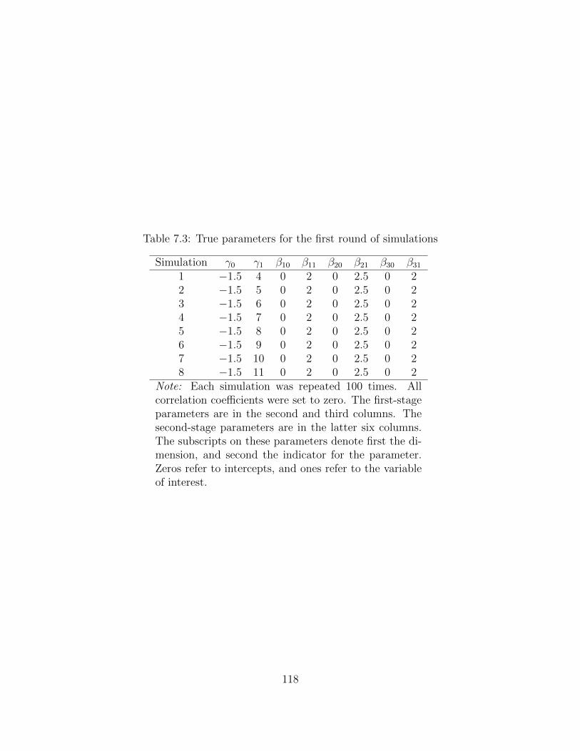
Table 7.3: True parameters for the first round of simulations

Simulation γ0 γ1 β10 β11 β20 β21 β30 β311 −1.5 4 0 2 0 2.5 0 22 −1.5 5 0 2 0 2.5 0 23 −1.5 6 0 2 0 2.5 0 24 −1.5 7 0 2 0 2.5 0 25 −1.5 8 0 2 0 2.5 0 26 −1.5 9 0 2 0 2.5 0 27 −1.5 10 0 2 0 2.5 0 28 −1.5 11 0 2 0 2.5 0 2

Note: Each simulation was repeated 100 times. Allcorrelation coefficients were set to zero. The first-stageparameters are in the second and third columns. Thesecond-stage parameters are in the latter six columns.The subscripts on these parameters denote first the di-mension, and second the indicator for the parameter.Zeros refer to intercepts, and ones refer to the variableof interest.

118

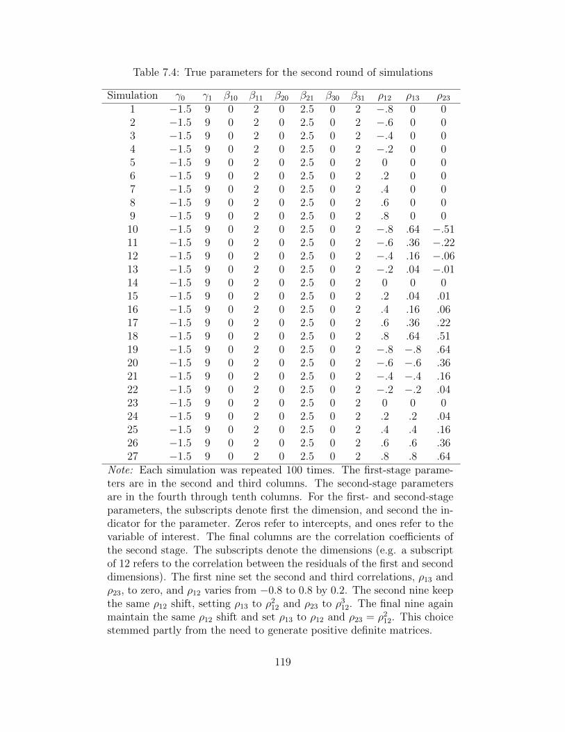
Table 7.4: True parameters for the second round of simulations

Simulation γ0 γ1 β10 β11 β20 β21 β30 β31 ρ12 ρ13 ρ231 −1.5 9 0 2 0 2.5 0 2 −.8 0 02 −1.5 9 0 2 0 2.5 0 2 −.6 0 03 −1.5 9 0 2 0 2.5 0 2 −.4 0 04 −1.5 9 0 2 0 2.5 0 2 −.2 0 05 −1.5 9 0 2 0 2.5 0 2 0 0 06 −1.5 9 0 2 0 2.5 0 2 .2 0 07 −1.5 9 0 2 0 2.5 0 2 .4 0 08 −1.5 9 0 2 0 2.5 0 2 .6 0 09 −1.5 9 0 2 0 2.5 0 2 .8 0 010 −1.5 9 0 2 0 2.5 0 2 −.8 .64 −.5111 −1.5 9 0 2 0 2.5 0 2 −.6 .36 −.2212 −1.5 9 0 2 0 2.5 0 2 −.4 .16 −.0613 −1.5 9 0 2 0 2.5 0 2 −.2 .04 −.0114 −1.5 9 0 2 0 2.5 0 2 0 0 015 −1.5 9 0 2 0 2.5 0 2 .2 .04 .0116 −1.5 9 0 2 0 2.5 0 2 .4 .16 .0617 −1.5 9 0 2 0 2.5 0 2 .6 .36 .2218 −1.5 9 0 2 0 2.5 0 2 .8 .64 .5119 −1.5 9 0 2 0 2.5 0 2 −.8 −.8 .6420 −1.5 9 0 2 0 2.5 0 2 −.6 −.6 .3621 −1.5 9 0 2 0 2.5 0 2 −.4 −.4 .1622 −1.5 9 0 2 0 2.5 0 2 −.2 −.2 .0423 −1.5 9 0 2 0 2.5 0 2 0 0 024 −1.5 9 0 2 0 2.5 0 2 .2 .2 .0425 −1.5 9 0 2 0 2.5 0 2 .4 .4 .1626 −1.5 9 0 2 0 2.5 0 2 .6 .6 .3627 −1.5 9 0 2 0 2.5 0 2 .8 .8 .64

Note: Each simulation was repeated 100 times. The first-stage parame-ters are in the second and third columns. The second-stage parametersare in the fourth through tenth columns. For the first- and second-stageparameters, the subscripts denote first the dimension, and second the in-dicator for the parameter. Zeros refer to intercepts, and ones refer to thevariable of interest. The final columns are the correlation coefficients ofthe second stage. The subscripts denote the dimensions (e.g. a subscriptof 12 refers to the correlation between the residuals of the first and seconddimensions). The first nine set the second and third correlations, ρ13 andρ23, to zero, and ρ12 varies from −0.8 to 0.8 by 0.2. The second nine keepthe same ρ12 shift, setting ρ13 to ρ212 and ρ23 to ρ312. The final nine againmaintain the same ρ12 shift and set ρ13 to ρ12 and ρ23 = ρ212. This choicestemmed partly from the need to generate positive definite matrices.

119

7.18.3 Presidential Campaigns in Mexico

To better assess how our inferences would be changed if the main application in the chapterdid not allow for correlations, I present a model that restricts the correlation parameters tobe zero. This is similar to the simulation exercises comparing ZIMVOP to an uncorrelatedmultivariate probit. The first-step estimates are nearly identical between models, but thesecond-step estimates vary fairly substantially, with some estimates reliable in one modeland not in the other. A main parameter of interest, Previous vote, though not reliable atthe 95% level for the PRI, is not even reliable at the 90% in the second model. The results,presented next to each other, are shown in Figure 7.31. Not only would we be losing theinformation provided by the correlation estimates, the simulations suggest that we shouldtrust the posteriors from ZIMVOP.

120

Figure 7.31: Comparing ZIMVOP to a model without correlations on the main application

−2 0 1 2 3 4

Second Step CoefficientEstimates, Original

Estimate

PANPRIPRD

Previous Vote

Coparty Mayor

Concurrent

Population Size

Gira

2012 Dummy

−2 0 1 2 3 4

Second Step CoefficientEstimates, No Correlation

Estimate

PANPRIPRD

Previous Vote

Coparty Mayor

Concurrent

Population Size

Gira

2012 Dummy

Note: The second-step results from ZIMVOP are presented on the left panel, and the resultsnot allowing correlations is on the right panel. As can be seen, the posteriors are fairlydifferent. Not only would we be losing the information provided by the correlation estimates,the simulations suggest that we should trust the posteriors from ZIMVOP.

121

7.19 Executive Moderation and Public Approval in Latin

America Supplementary Information

Below are the tables of the β estimates for all of the GPR models run in the fourth chapter.I suppress the estimates for the presidential indicators for space.

Table 7.5: Posterior β estimates for the first hypothesis

mean 2.5% 97.5%

Executive moderation 0.328 0.097 0.567GDP growth 0.362 −0.005 0.736Inflation (logged) −0.249 −1.012 0.585Spending 0.068 −1.114 1.185Trade 0.580 −0.939 2.215

Table 7.6: Posterior β estimates for the second hypothesis

mean 2.5% 97.5%

Executive moderation −0.052 −0.340 0.259Extremity 0.760 0.252 1.220Executive moderation × Extremity 0.217 0.009 0.418GDP growth 0.362 0.064 0.691Inflation (logged) 0.135 −0.682 0.901Spending 0.695 −0.561 1.875Trade 0.308 −1.090 1.613

Table 7.7: Posterior β estimates for the third hypothesis

mean 2.5% 97.5%

Election year −0.186 −0.692 0.317GDP growth 0.306 −0.068 0.664Inflation (logged) −0.156 −0.992 0.684Spending −0.394 −1.589 0.835Trade −0.082 −1.832 1.541

122

Table 7.8: Posterior β estimates for the fourth hypothesis

mean 2.5% 97.5%

Election year −0.135 −0.484 0.203Extremity 1.271 0.956 1.604Election year × Extremity −0.235 −0.449 −0.018GDP growth 0.274 0.014 0.535Inflation (logged) 0.449 −0.262 1.087Spending 0.660 −0.450 1.752Trade −0.818 −2.092 0.331

123