Advanced International Macroeconomics and Finance OUP Book, Chapter … · 2014-04-01 · Advanced...

Advanced International Macroeconomics and FinanceOUP Book, Chapter 3:

Dynamic Macroeconomic Approaches tothe Balance of Payments and the Exchange Rate

Miguel A. León-Ledesma∗ and Alexander Mihailov†

January 24, 2011‡

Abstract

Having explored various implications of the comparative statics analysis in thepreceding chapter, we now turn to deterministic (i.e., not stochastic) dynamicmacroeconomic models of balance of payments adjustment and exchange rate deter-mination. These models are based on postulated aggregate relationships in open-economy environments and are dynamic insofar they are solved under perfect fore-sight, which is the strongest form of rational expectations. After briefly introducingthe concept of rational expectations in section 1, we first review in section 2 thestock, or asset (market), model of the BoP and the NER under flexible prices. Thisis the monetary approach developed in the late 1960s and the 1970s. Section 3 thenswitches to sticky prices and presents in detail a very influential article, the Dorn-busch (1976) model of exchange rate overshooting, in fact, a dynamic version of thestatic Mundell-Fleming framework studied in chapter 2. It is, certainly, due to thesignificant contribution made by each of these three authors that this general set-upand its extensions in the subsequent literature are sometimes called the Mundell-Fleming-Dornbusch tradition (or paradigm) in international macroeconomics. Weconclude the chapter by reviewing, in section 4, some empirical implications of theexchange rate models discussed, considering in particular the random walk hypoth-esis of the exchange rate in Meese and Rogoff (1983 a, b) and later work. Asa technical complement underlying the chapter, backward and forward solutionsto stochastic difference equations as well as the general solution to deterministichomogeneous differential equations are illustrated with some detail in appropriatecontexts; also, the difference among and the rationale for perfect foresight, static,adaptive and rational expectations as well as mean error (ME), mean absolute error(MAE) and root mean square error (RMSE) of forecasts are analytically clarified.

∗Department of Economics, Keynes College, University of Kent, Canterbury, Kent, CT2 7NP, UK;[email protected]

†Department of Economics, University of Reading, Whiteknights, Reading RG6 6AA, andDepartment of Economics, University of Warwick, Coventry, CV4 7AL, United Kingdom;[email protected].

‡Comments welcome. All remaining errors are ours.

Contents

1 The Rational Expectations Revolution 11.1 Expectations and Economic Behaviour . . . . . . . . . . . . . . . . . . . 11.2 A Basic Analytical Taxonomy of Modelling Expectations in Economics . 1

1.2.1 Perfect Foresight . . . . . . . . . . . . . . . . . . . . . . . . . . . 11.2.2 Naive or Static Expectations . . . . . . . . . . . . . . . . . . . . 21.2.3 Adaptive Expectations . . . . . . . . . . . . . . . . . . . . . . . . 21.2.4 Rational Expectations . . . . . . . . . . . . . . . . . . . . . . . . 3

1.3 Muth (1961) and the Rational Expectations Revolution in Macroeconomics 4

2 Flexible-Price Stock Approach under Perfect Foresight: The MonetaryModel 42.1 The Monetary Approach to the Balance of Payments (Peg) . . . . . . . 6

2.1.1 Origins: The Classical (Humean) Price-Specie-Flow Mechanism . 62.1.2 Main Assumptions . . . . . . . . . . . . . . . . . . . . . . . . . . 72.1.3 Set-Up and Derivation of Key Result . . . . . . . . . . . . . . . . 72.1.4 Analysis and Interpretation . . . . . . . . . . . . . . . . . . . . . 9

2.2 The Monetary Approach to the Exchange Rate (Float): The MonetaryModel . . . . . . . . . . . . . . . . . . . . . . . . . . . . . . . . . . . . . 102.2.1 Set-Up and Derivation of Key Results . . . . . . . . . . . . . . . 102.2.2 General Forward-Looking Solution . . . . . . . . . . . . . . . . . 112.2.3 No-Bubbles Solution . . . . . . . . . . . . . . . . . . . . . . . . . 122.2.4 Rational Bubbles . . . . . . . . . . . . . . . . . . . . . . . . . . . 13

3 Sticky-Price Models of Exchange Rate Dynamics under Perfect Fore-sight: The Dornbusch (1976) Overshooting Model 153.1 Stylised Facts the Model was Designed to Explain . . . . . . . . . . . . 153.2 Key Assumptions of the Model . . . . . . . . . . . . . . . . . . . . . . . 16

3.2.1 General Assumptions . . . . . . . . . . . . . . . . . . . . . . . . . 163.2.2 Capital Mobility and Exchange-Rate Expectations Formation . . 173.2.3 Money Market Structure and Equilibrium . . . . . . . . . . . . . 173.2.4 Goods Market Structure and Equilibrium . . . . . . . . . . . . . 19

3.3 Model Equilibrium and Transition Paths . . . . . . . . . . . . . . . . . . 213.3.1 Graphical Analysis . . . . . . . . . . . . . . . . . . . . . . . . . . 213.3.2 Alternative Ways of Goods Market Clearing . . . . . . . . . . . . 233.3.3 Consistent Expectations . . . . . . . . . . . . . . . . . . . . . . . 23

3.4 Model Main Result: Exchange Rate Overshooting . . . . . . . . . . . . 24

4 Empirics of the Nominal Exchange Rate and the Random Walk Hy-pothesis 274.1 Meese and Rogoff (1983): The Exchange Rate Disconnect Puzzle . . . . 274.2 Explaining the Meese and Rogoff (1983) Results . . . . . . . . . . . . . 30

4.2.1 Econometric Issues . . . . . . . . . . . . . . . . . . . . . . . . . . 304.2.2 Engel and West (2005): The Exchange Rate as a Near-Random

Walk . . . . . . . . . . . . . . . . . . . . . . . . . . . . . . . . . . 344.2.3 Where Do We Stand? . . . . . . . . . . . . . . . . . . . . . . . . 35

List of Figures

1 The Dornbusch Model: Long-Run Equilibrium and Transition Paths . . 222 The Dornbusch Model: Exchange Rate Overshooting . . . . . . . . . . . 24

List of Tables

1 The Meese-Rogoff Results . . . . . . . . . . . . . . . . . . . . . . . . . . 312 Long-Horizon Forecasts . . . . . . . . . . . . . . . . . . . . . . . . . . . 33

Advanced International Macroeconomics and Finance OUP Book, Chapter 3 1

1 The Rational Expectations Revolution

This first section has the purpose to introduce the concept of rational expectations (RE)and to compare it analytically with a few alternative ways of modelling expectations thathave been common in macroeconomics.

1.1 Expectations and Economic Behaviour

The behaviour of economic agents is based on certain expectations concerning the futurelevel or evolution of relevant variables or processes. This fact differentiates social fromnatural sciences as acknowledged by Evans and Honkapohja (2001): “Modern economictheory recognises that the central difference between economics and natural scienceslies in the forward-looking decisions made by economic agents.” (p. 5). They furtherascertain that expectations influence the time path of the macroeconomy, and vice versa,so that there is a profound two-sided relationship, a challenge to modellers.

Evans and Honkapohja (2001) also indicate that systematic economic theories at-tributing a major role to expectations can be first seen in Thornton (1802) and Cheysson(1887). Classical economists implicitly applied perfect foresight, and Marshall is cred-ited with the concept of static expectations. Long-run expectations of prospective yieldsand asset prices are main themes in Keynes (1936), while in the 1950s and 1960s adap-tive expectations or related lagged adjustment mechanisms had become widespread inmacroeconomic models. Muth (1961) is the seminal paper which explicitly defines ra-tional expectations in an economic context. His impact on how to write down andsolve economic models under assumptions for rationality of forward-looking agents wassomewhat delayed, but crucial indeed for the profession. Since Lucas (1972) and Sar-gent (1973) introduced and extended his RE methodology to macroeconomics, it hasbeen the dominant feature of dynamic theoretical analysis. Rogoff (2002) attributes toBlack (1973) the first consideration of rational expectations in an international financecontext.1

Before moving to the perfect foresight models in the next sections, we first ‘catalogue’the key types of expectations having been employed in economics in a taxonomy allowingclear comparison by means of analytical expressions.

1.2 A Basic Analytical Taxonomy of Modelling Expectations in Eco-nomics

Following Evans and Honkapohja (2001), the major types of expectations that have beenimportant in economic modelling are characterised here by their defining formulas.

1.2.1 Perfect Foresight

Perfect foresight is a common assumption in earlier RE models endowing economicagents with superhuman powers. Perfect foresight, in fact, means that these agentsmake no mistakes in predicting the future value of a variable of interest. I.e., theexpected value, pet , of a variable p (say, some price) at time t is simply the actual (orrealised) value of the same variable:

1Evans (1985) and Evans and Honkapohja (1995, 2001) developed this line of research further tobounded rationality that incorporates statistical learning.

2 León-Ledesma and Mihailov (January 24, 2011)

pet = pt.

This is, naturally, not at all a realistic assumption. Yet it disciplines the researcherto restrict attention to the study of behaviour that is model-consistent, as we makeclearer below. Moreover, before better techniques for handling analytically expectationsin macroeconomics were developed by the late 1970s, perfect foresight had been theprevalent RE hypothesis assumed.

1.2.2 Naive or Static Expectations

Static (or naive) expectations imply that the expected value of a variable p at time tis the actual (or realised) value of the same variable at the previous date (i.e., at timet− 1):

pet = pt−1.

Static expectations thus predict no change.

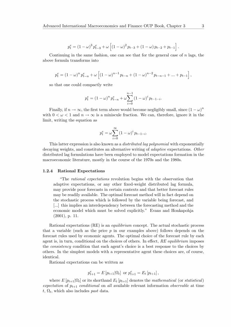
1.2.3 Adaptive Expectations

This type of modelling expectations appears to have been explicitly introduced in Cagan(1956). It implies that the expected value of a variable p at time t is the expected value ofthe same variable p at time t−1 plus a term accounting for the forecast error pt−1−pet−1at time t− 1 (an error correction term):

pet = pet−1 + ω¡pt−1 − pet−1

¢.

The weight on the forecast error is given above by the constant 0 < ω < 1 (yet, moregenerally, weights can change too, so that ωt then would be the right notation). Theabove equation can be solved backwards for pet . Write it as

2

pet = (1− ω) pet−1 + ωpt−1

and start by lagging it one period (compare the subscripts):

pet−1 = (1− ω) pet−2 + ωpt−2. (1)

Then substitute for pet−1 from the latter into the former expression:

pet = (1− ω)£(1− ω) pet−2 + ωpt−2

¤| z =pet−1

+ ωpt−1,

pet = (1− ω)2 pet−2 + ω [(1− ω) pt−2 + pt−1] . (2)

Now lag equation (1) by one period,

pet−2 = (1− ω) pet−3 + ωpt−3

and substitute for pet−2 from the latter expression into (2) to obtain:

2An alternative notation to implement the same solution in a more compact writing makes use ofthe lag operator.


pet = (1− ω)3 pet−3 + ωh(1− ω)2 pt−3 + (1− ω) pt−2 + pt−1

i.

Continuing in the same fashion, one can see that for the general case of n lags, theabove formula transforms into

pet = (1− ω)n pet−n + ωh(1− ω)n−1 pt−n + (1− ω)n−2 pt−n−1 + ...+ pt−1

i,

so that one could compactly write

pet = (1− ω)n pet−n + ωn−1Xi=0

(1− ω)i pt−1−i.

Finally, if n→∞, the first term above would become negligibly small, since (1− ω)n

with 0 < ω < 1 and n → ∞ is a miniscule fraction. We can, therefore, ignore it in thelimit, writing the equation as

pet = ω∞Xi=0

(1− ω)i pt−1−i.

This latter expression is also known as a distributed lag polynomial with exponentiallydecaying weights, and constitutes an alternative writing of adaptive expectations. Otherdistributed lag formulations have been employed to model expectations formation in themacroeconomic literature, mostly in the course of the 1970s and the 1980s.

1.2.4 Rational Expectations

“The rational expectations revolution begins with the observation thatadaptive expectations, or any other fixed-weight distributed lag formula,may provide poor forecasts in certain contexts and that better forecast rulesmay be readily available. The optimal forecast method will in fact depend onthe stochastic process which is followed by the variable being forecast, and[...] this implies an interdependency between the forecasting method and theeconomic model which must be solved explicitly.” Evans and Honkapohja(2001), p. 11.

Rational expectations (RE) is an equilibrium concept. The actual stochastic processthat a variable (such as the price p in our examples above) follows depends on theforecast rules used by economic agents. The optimal choice of the forecast rule by eachagent is, in turn, conditional on the choices of others. In effect, RE equilibrium imposesthe consistency condition that each agent’s choice is a best response to the choices byothers. In the simplest models with a representative agent these choices are, of course,identical.

Rational expectations can be written as

pet+1 = E [pt+1|Ωt] or pet+1 = Et [pt+1] ,

where E [pt+1|Ωt] or its shorthand Et [pt+1] denotes the mathematical (or statistical)expectation of pt+1 conditional on all available relevant information observable at timet, Ωt, which also includes past data.


1.3 Muth (1961) and the Rational Expectations Revolution inMacroe-conomics

Muth (1961) was the first to formulate the rational expectations hypothesis as a theory ofexpectations formation and to show that its implications are roughly consistent with therelevant data. In essence, he defined rational expectations, or “informed predictions offuture events”, as “the same as the predictions of the relevant economic theory”, that is,in the sense of model-consistency. More precisely, the hypothesis states: “expectationsof firms (or, more generally, the subjective probability distribution of outcomes) tend tobe distributed, for the same information set, about the prediction of the theory (or the‘objective’ probability distributions of outcomes).” Muth (1961), p. 316.

As clarified in the original article, the RE hypothesis asserts three propositions:

1. The economic system does not waste scarce information.

2. Expectations formation depends specifically on the structure of the relevant systemdescribing the economy.

3. Public predictions will have no substantial effect on the operation of the economicsystem, unless based on inside information.

After formulating the RE hypothesis, Muth (1961) applied it to a simple economicenvironment, introducing the basic mathematics to handle such analysis.

The overwhelming influence of Muth’s (1961) RE methodology on the mainstreamof contemporary macroeconomics has commonly been termed the rational expectationsrevolution. Starting with Lucas (1972) and Sargent (1973) in closed-economy set-ups,and with Black (1973) in an open-economy framework, the profession has been accu-mulating better techniques to address expectations formation and to analyse its impactin various economic environments, up until the current proliferation of the literature onbounded rationality with statistical learning, to which we shall briefly return by the endof this book.3

2 Flexible-Price Stock Approach under Perfect Foresight:The Monetary Model

With the notions of RE and perfect foresight now defined, this section goes on to outlinein more detail the so-called stock approach to BoP adjustment and NER determination insubsections 2.1 and 2.2.4 It is important to understand a major difference in perspectivewith respect to chapter 2, which focused on flow approaches. The models that belongto the group of the asset (market) or stock approaches to the BoP and/or the NERemphasise the view that flow adjustments of financial variables are ultimately driven

3Recent macroeconomics literature within the maximizing agents framework has also critizised thewidespread use of the basic notion of RE in Dynamic Stochastic General Equilibrium (DSGE) models.This is the case, for instance, in Sim’s (2003) idea of “rational inattention”.

4We focus in this chapter on the monetary model only because of its relevance for modern researchin international macroeconomics and the lasting influence it has exerted. There is, however, a (nowsomewhat obsolete) literature on “portfolio balance models” (PBMs) of the exchange rate. These includestock-flow approaches such as Branson and Buiter (1983) for general equilibrium and Branson andHenderson (1985) for partial equilibrium. A concise summary of PBMs can be found in Sarno andTaylor (2002).


by the adjustment of the underlying desired stocks of assets held in various currencydenominations as part of wealth portfolios of economic agents. The stock approachesdo not, however, totally ignore the flow of funds arising from trade, highlighted in themodels of chapter 2. Rather, they point to the fact that there is much more to flowadjustment, i.e., in addition to flow adjustment, and that the magnitude of stocks is gen-erally much higher than the magnitude of flows, so that even a small percentage changein stock-supply or stock-demand may generate a large percentage change of correspond-ing flows. Moreover, the stock and flow adjustments are, by definition, influencing eachother, so another term — and approach — commonly employed in analysis of the BoPand/or the NER has been termed stock-flow models.

The rationale for the shift of emphasis from flow to asset approaches in academicresearch can also partly be seen as a consequence of institutional changes in the globalmonetary system, with an increasing capital mobility and deregulation of internationalfinancial transactions after the demise of Bretton Woods. As Lindbeck (1976), p. 139,duly remarks, such changes have led to different conceptual interpretations of the re-lations between the current (CA) and financial (KA) accounts of the BoP. In analysesbefore World War II, long-term capital movements were usually assumed to be deter-mined by differentials among real rates of return on physical assets; consequently, theCA was assumed to adjust via changes in relative prices, stock of assets, exchange ratesor income. During the Bretton Woods system of fixed parities under heavily regulatedcapital flows, largely inconvertible currencies and small stocks of foreign claims relativeto the flows of trade, the emphasis in analyses of the BoP and the NER moved to theCA; the KA, then, was assumed to adjust to the state of the CA, via capital flows in-duced by interest rate differentials or political control. Lindbeck (1976) concludes thatthe increasing size of the stock of foreign financial assets and (related) capital flows sincethe early 1970s has once again modified the focus through which researchers analyse theinteraction between the CA and the KA. In line with the asset approach, establishingitself more firmly since about that same time, the most important short-run effects onthe BoP and the NER were asserted to come from shifts in stock-demand and stock-supply unrelated to the current account. However, these effects were accumulating onthe current account as time passed by, and with subsequent feedbacks on the marketsfor assets and foreign exchange.5

Models along the above lines that view the exchange rate as an asset price under per-fect foresight were developed employing assumptions of both flexible prices (this section)and sticky prices (section 3). Among the flexible-price perfect foresight models, our focusis on the most prominent one, the monetary model of the exchange rate. It is often thecase, and we shall note that in this book on several occasions, that open-economy mod-els are in essence extensions of corresponding, methodologically similar, closed-economymodels. The monetary model under flexible prices presented further down is, thus, anextension of the empirical set-up of Cagan (1956) analysing hyperinflations in a closedeconomy.6

5See Johnson (1977) for an overview of the different approaches to the BoP up to the monetarymodel.

6For more details on the Cagan (1956) model in its initial closed-economy version and later open-economy extension, see the original contribution and chapter 8 in Obstfeld and Rogoff (1996).


2.1 The Monetary Approach to the Balance of Payments (Peg)

The monetary approach to the balance of payments was developed in the 1960s, in partwithin the research department of the IMF under the intellectual leadership of JacquesPolak and in the context of the Bretton Woods system of fixed exchange rates. With itscollapse, the approach was extended to cover the case of flexible exchange rates, thusbecoming one of the major theories of NER determination. The monetary approach tothe balance of payments is described in a comprehensive manner in the volume editedby Frenkel and Johnson (1976). In this and the next subsections, we present its twoversions, for a regime of peg or float, respectively.7

No matter that the monetary approach to the BoP found its accomplished form inthe 1970s, its proponents, e.g., Frenkel (1976), have claimed that the intellectual originsof this theory go back to Hume (1752), Wheatley (1803), Ricardo (1821) and to Cassel’s(1918, 1921) revival of ideas of the Salamanca School in the 16-th century related to theproposition of purchasing power parity (PPP). The Casselian approach to PPP has laterbeen articulated by Samuelson (1964) in the context of a generalisation of the law of oneprice (LOP) ensured by commodity arbitrage for all internationally traded goods. PPPis definitely violated in the short run, but tends to be a long-run equilibrium concept towhich nominal exchange rates gravitate.8 That is why it is often an ingredient in manyeconomic models, including the monetary approach, especially as a long-term condition.For this reason, and also because of the assumption of flexible prices, the monetarymodel should be understood as a benchmark long-run equilibrium model.

2.1.1 Origins: The Classical (Humean) Price-Specie-Flow Mechanism

In summary, the classical theory of balance of payments adjustment under the goldstandard, building on ideas of Hume (1752), is as follows. A surplus in the BoP (or,more precisely, the current account) causes an inflow of gold. The gold inflow increasesthe price level. This is because of two mechanisms: (i) the link between gold reserves andthe amount of money in circulation under the gold standard due to (full) convertibility of(paper) money into metal equivalent; (ii) the link between money and prices originatingin the quantity theory of money (QTM) with the economy operating at full employmentwhich states: MtV = PtY . That is, if Mt ↑, then Pt ↑ too, since the income velocity ofmoney V and real output Y are assumed constant by the QTM. Hence, as the goodsof the surplus country become relatively more expensive in the international market,the increased demand for imports by residents and the reduced demand for exportsby nonresidents lead to a gradual reduction of the initial trade surplus. Analogouslogic applies to the case of a CA deficit. Thus, the so-called price-specie(=gold)-flowmechanism ensures automatically BoP equilibrium under the gold standard.

A different perspective on the same process is based on the notion of the optimumor desired distribution of the stock of specie (gold) among all countries in the world.Any BoP disequilibrium, which is a flow disequilibrium, is therefore determined by theunderlying stock disequilibrium, i.e., a distribution of the stock of gold available in theworld which does not coincide with the desired one, ensuring BoP equilibrium.

The important point of Hume’s price-specie-flow mechanism is that the ultimatecause of balance of payments disequilibria is to be found in money stock disequilibria:

7Our exposition is based on original articles, e.g., Lindbeck (1976), Frenkel (1976) and Mussa (1976),as well as on Mark (2001), chapter 3, and Gandolfo (2001), parts of chapters 12, 13 and 15.

8Chapter 6 will discuss the evidence on PPP.


a divergence of the quantity of money (gold) supplied and the quantity demanded byeach country’s residents. It is from such considerations that the monetary approach tothe BoP took its source.

2.1.2 Main Assumptions

1. PPP is a key assumption in the monetary approach, justified as an aggregation ofthe law of one price (LOP) in the markets for goods and services.

2. UIP is assumed to hold as well, so we have perfect substitutability between homeand foreign assets.

3. In contrast to the flow approaches to BoP adjustment we studied thus far, allprices are assumed flexible under the monetary approach.

4. Again, opposite to the flow models explored earlier, the focus of the monetaryapproach is on conditions for stock equilibrium in the money market: the BoP isessentially a monetary phenomenon, and should therefore be analysed in terms ofadjustment of money stocks.

5. Production is assumed at the level of full employment, so real income is fixed.This assumption, together with flexible prices ensure no short-run output-inflationtrade-off (i.e. a vertical Phillips Curve).

6. A stable money demand function is taken to exist.

7. We will consider below the small open-economy case, although two-country ver-sions of the model are straightforward to write down.

The monetary approach to BoP adjustment (under fixed exchange rates) or to NERdetermination (under flexible exchange rates) has been widely used for policy analy-sis. We shall see in later chapters that many of its predictions are confirmed by morecomplicated optimising models, both in flexible-price and sticky-price environments.

As is customary in the literature, the model will be presented in a notation dis-tinguishing between levels of the variables, denoted by upper -case letters, and corre-sponding (natural) logarithms of the variables, denoted by lower -case letters (except forinterest rates, which are themselves in (net) per-unit terms and are in levels).

2.1.3 Set-Up and Derivation of Key Result

Using the notation we introduced so far, we start by writing the definition of the moneysupply, in levels:

MSt ≡ μMBt ≡ μ (DCt + IRt) , (3)

where μ ≡ E[MSt]E[MBt]

is the money multiplier, assumed constant.We next proceed to a logarithmic expansion of the money supply and its components

about their mean values. Such first-order expansion of (3) could be done as follows.Taking expectations from both sides of (3),

E [MSt] ≡ μE [DCt] + μE [IRt] ,


subtracting the above equation from (3) and rearranging, yields:

MSt −E [MSt] ≡ μ (DCt −E [DCt]) + μ (IRt −E [IRt]) .

Dividing through by E [MSt],

MSt −E [MSt]

E [MSt]≡ μ (DCt −E [DCt])

E [MSt]+

μ (IRt −E [IRt])

E [MSt],

substituting for the definition of μ and rewriting gives:

MSt −E [MSt]

E [MSt]≡ (DCt −E [DCt])

E [MBt]+(IRt −E [IRt])

E [MBt],

MSt −E [MSt]


E[DCt]E[DCt]

E [MBt]+(IRt −E [IRt])E[IRt]E[IRt]

E [MBt],

Defining θ ≡ E[IRt]E[MBt]

and, hence, (1− θ) ≡ E[DCt]E[MBt]

, we get, by substitution:

MSt −E [MSt]


E[DCt]1−θ

+(IRt −E [IRt])

E[IRt]θ

,

MSt −E [MSt]

E [MSt]≡ (1− θ)

(DCt −E [DCt])

E [DCt]+ θ

(IRt −E [IRt])

E [IRt].

Now, since for a random variable Zt,Zt−E[Zt]E[Zt]

≈ ln (Zt) − ln (E [Zt]), ignoring anarbitrary constant depending on the mean values, we can write the money supply in thecorresponding logarithms:

mst ≈ (1− θ) dt + θirt. (4)

A standard transactions and speculation motive gives rise to the following demandfor money function in levels:

Mdt

Pt= Y φ

t e−λιte t .

Written in logarithms, i.e., taking logs from both sides, this yields

mdt − pt = φyt − λιt + t, (5)

with 0 < φ < 1 being the income elasticity of money demand, λ > 0 the interestsemi-elasticity (since the interest rate is not in natural logs, as noted earlier) of moneydemand and the error term assumed independently and identically distributed (iid) with

zero mean and constant variance, tiid∼ ¡0, σ2¢.

We next use PPP and UIP, as assumed within the monetary approach framework.Since the exchange rate is fixed, say at s, PPP implies (in logs as below, from

Pt = SP ∗t in levels) that the domestic price level in the SOE is determined by theexogenous foreign (RoW) price level:

pt = s+ p∗t . (6)


Moreover, assuming a credible peg, market participants do not expect a change inthe NER, i.e., Et [St+1] = St = S = const for any t (hence ln Et[St+1]

St= ln S

S= ln 1 = 0),

so that UIP reduces (taking log approximations) to

ιt = ι∗t , (7)

which implies that the interest rate in the SOE is equal to the exogenous foreign(RoW) interest rate.

We finally assume that the money market is continuously in equilibrium, so that wecan equate the supply of money (4) to the demand for money (5):

(1− θ) dt + θirt = pt|z=s+p∗t

+ φyt − λ ιt|z=ι∗t

+ t.

Rearranging, one obtains:

θirt = s+ p∗t + φyt − λι∗t + t| z =md

t

− (1− θ) dt. (8)

2.1.4 Analysis and Interpretation

Equation (8) summarises the main insights of the monetary approach to the balance ofpayments, or, which is the same, of the monetary model (of the balance of payments)under peg. It is evident from the money demand function (5) that if the SOE in questionexperiences any of the following:

• positive income growth, yt ↑;• declining interest rates, ιt ↓;• rising prices, pt ↑;the demand for nominal money balances will grow, md

t ↑.Equation (8) further shows that if this increased demand for money is not satisfied

by an accommodating increase in domestic credit, dt, so that mdt > (1− θ) dt in (8),

the public will obtain the additional money it desires to hold by running an overallBoP surplus, i.e., an increase in international reserves, irt; if, on the other hand, thecentral bank engages in a domestic credit expansion that exceeds the growth of moneydemand, so that md

t < (1− θ) dt in (8), the public will eliminate the excess supply ofmoney (it does not wish to hold) by spending or investing it abroad and thus runninga(n overall) BoP deficit, i.e., a decrease in international reserves. Consequently, themoney supply, ms

t ≡ (1− θ) dt + θirt, in the monetary model under peg is endogenous,that is, determined by expression (8).

Note that this endogeneity of money supply is also a common feature of the Mundell-Fleming model analysed in chapter 2. In essence, the conclusion that under fixed ex-change rates the monetary authority loses control of domestic credit (the policy instru-ment in this model) remains unchanged. Note also that, with fixed exchange rates, thecorrection of any disequilibrium in the BoP induced by, say, a shock to money demand( t) is brought about by an adjustment of the level of reserves (the specie-flow). In otherwords, the stock disequilibrium in the money market is corrected by a flow adjustmentof reserves.


2.2 The Monetary Approach to the Exchange Rate (Float): The Mon-etary Model

Changing the assumption of a peg with the alternative of a flexible exchange rate regimetransforms the above model into what has become known as the monetary approach tothe (nominal) exchange rate.9

The similarities between the monetary model under peg and under float are manyindeed. However, there are also differences, originating in the alternative assumptionabout the NER regime: these differences are evident below in the expressions for PPPand UIP, which still hold but in a modified analytical form. We write the model assumingtwo countries, Home and Foreign (RoW). We also assume that the pair of moneydemand equations has identical parameters for the two countries.

2.2.1 Set-Up and Derivation of Key Results

Under float, the money supply is exogenous, i.e., it is determined by the monetaryauthority in each of the countries, since the central bank does not need to target acertain value of the NER. Equilibrium in the money market in Home and Foreign isthen given by the pair of equations:

mt − pt| z supply of real balances in H

= φyt − λιt| z demand for real balances in H

, (9)

m∗t − p∗t| z supply of real balances in F

= φy∗t − λι∗t| z demand for real balances in F

. (10)

International capital market equilibrium is determined by UIP, now allowing forexpected depreciation under the float regime (i.e., with ln Et[St+1]

St= lnEt [St+1]−lnSt ≡

Et [st+1]− st):

ιt − ι∗t = Et [st+1]− st. (11)

PPP relates the price levels in the two economies through the exchange rate, giventhat LOP holds for the individual products ensuring equilibrium in the market for goodsvia arbitrage:

st = pt − p∗t . (12)

A usual simplification of the notation at this point, which allows certain interpreta-tion as to what constitutes the (economic) fundamentals of the exchange rate, is:

ft ≡ (mt −m∗t )− φ (yt − y∗t ) , (13)

where ft is the vector of fundamentals that determine the exchange rate multipliedby their respective coefficients (vector [1,−φ]0).

Substituting (9), (10) and then (11) and (13) into (12) and rearranging, we get:

st = mt − φyt + λιt| z =pt, from (9)

− (m∗t − φy∗t + λι∗t )| z =p∗t , from (10)

,

9Obstfeld and Rogoff (1996), pp. 526-530, also call the monetary model “the Cagan model”, inhonour of the mentioned early contribution by Cagan (1956) with application to hyperinflation.


st = (mt −m∗t )− φ (yt − y∗t )| z ≡ft, from (13)

+ λ (ιt − ι∗t )| z =Et[st+1]−st, from (11)

,

st = ft + λ (Et [st+1]− st) . (14)

If we now solve for st we obtain:

st = ft + λEt [st+1]− λst,

(1 + λ) st = ft + λEt [st+1] ,

st =1

1 + λ| z ≡γ

ft +λ

1 + λ| z ≡(1−γ)

Et [st+1] ,

st = γft + (1− γ)Et [st+1] . (15)

(15) is the central equation in the monetary model. It is a first-order dynamic-stochastic difference equation that states that the current value of the exchange rate isa function of future expected values of the exchange rate. From the composition of thefundamentals term ft it is clear that high relative money growth in Home, mt−m∗t > 0,leads to a depreciation of the Home currency, st ↑, while high relative income growth,yt − y∗t > 0, tends to appreciate it, st ↓. In the long-run equilibrium or steady state,when st = Et [st+1], we then have that st = ft.

2.2.2 General Forward-Looking Solution

Equation (15) can be solved forward for the exchange rate, under an (implicit or explicit)assumption of rational expectations.10 This is done by first writing (15) one periodforward,

st+1 = γft+1 + (1− γ)Et+1 [st+2] ,

then taking expectations conditional on time t information,

Et [st+1] = γEt [ft+1] + (1− γ)Et [Et+1 [st+2]] ,

and using the law of iterated expectations,11 to obtain

Et [st+1] = γEt [ft+1] + (1− γ)Et [st+2] ,

by which we substitute Et [st+1] back into (15) to get

st = γft + (1− γ)(γEt [ft+1] + (1− γ)Et [st+2])| z =Et[st+1]

.

10Note the parallels in the algorithm with the backward solution for the expected price in the subsectionintroducing adaptive expectations earlier in the chapter.11Here meaning, in particular, that Et [Et+1 [st+2]] = Et [st+2]. That is, with the information set

available at time t, agents “expect to expect” in period t+ 1 exactly what they expect in period t.


Further rearranging, one could write

st = γ Et [ft] + (1− γ)Et [ft+1]+ (1− γ)2Et [st+2] ,

st = γ1X

j=0

(1− γ)jEt [ft+j ] + (1− γ)2Et [st+2] .

We can now repeat the same procedure by advancing time in (15) by two, three,four periods and so forth, say up to k periods ahead. The result will be the generalequivalent of the equation above:

st = γkX

j=0

(1− γ)jEt [ft+j ] + (1− γ)k+1Et [st+k+1] . (16)

2.2.3 No-Bubbles Solution

If now we let k → ∞, the second term in (16) will vanish, becoming negligible asymp-totically:12

limk→∞

(1− γ)kEt [st+k] = 0. (17)

Equation (17) is called in similar models a transversality condition (TVC). By im-posing it, we restrict the rate at which the exchange rate can grow asymptotically toobtain the unique fundamentals (or no-bubbles) solution:13

st = γkX

j=0

(1− γ)jEt [ft+j ] . (18)

(18) expresses the current period (t) exchange rate as the present discounted value(PDV) of expected future values of the fundamentals. That is, the current NER reflectsnot only the current value of the fundamentals, but all the future expected path offundamentals. Hence, the NER is a reflection of market participants’ expectations, justlike in finance theory of asset pricing. For the latter theory a stock price, for instance, isthe present discounted value of the firm’s expected dividends. Because of this similarity,the monetary model is sometimes referred to as the asset approach to the exchange rate.From the perspective of this approach, it is natural to expect the exchange rate to bemore volatile than fundamentals, just like the prices of assets such as stocks are morevolatile than the corresponding dividends, an issue directly addressed by the Dornbuschovershooting model to be analysed in section 3.

12Recall that 0 < (1−γ) ≡ λ1+λ < 1 because we have, by definition, restricted λ to be positive (λ > 0),

so that the interest semi-elasticity of money demand, −λ, is negative (i.e., a higher interest rate would,ceteris paribus, reduce the demand for money).13Note that the TVC will hold only if, as k→∞, (1−γ)k goes to zero faster than st+k goes to infinity

in expected value.


2.2.4 Rational Bubbles

If the TVC does not hold, the behaviour of the exchange rate will be governed in partby an (asymptotically) explosive bubble, bt, which will eventually dominate the fun-damentals.14 We can show why this is the case by assuming that the bubble evolvesaccording to a first-order autoregressive process (AR1), where the autoregressive coef-ficient (measuring persistence) is defined to be 1

1−γ and thus exceeds 1 (11−γ > 1 since

0 < 1− γ < 1), which means that the bubble process is explosive:

bt =1

1− γbt−1 + ξt, (19)

where ξtiid∼ N

³0, σ2ξ

´. We can now add the bubble process (19) to the fundamentals

solution (18) to obtain back the general solution of the first-order stochastic differenceequation for the exchange rate we started with, (15), but now assuming a bubble:

bst = st + bt. (20)

One can check that bst violates the TVC, by simply substituting (20) into (17):limk→∞

(1− γ)kEt [bst+k] = limk→∞

(1− γ)kEt [st+k]| z =0

+ limk→∞

(1− γ)kEt [bt+k]| z =bt

= bt 6= 0. (21)

To understand why bt = limk→∞

(1 − γ)kEt [bt+k] in the expression just above, solve

forward (19):

(1− γ)bt = bt−1 + (1− γ)ξt,

bt−1 = (1− γ)bt − (1− γ)ξt.

Taking expectation at t− 1:

Et−1 [bt−1] = (1− γ)Et−1 [bt]− (1− γ)Et−1 [ξt]| z =0

,

bt−1 = (1− γ)Et−1 [bt] .

Or, which is the same,

bt = (1− γ)Et [bt+1] .

Hence,

14The solution path for any variable yt defined by a first-order linear difference equation has a particularsolution (or integral) and a complementary function. The sum of these two constitutes the generalsolution. In the case of (16) the TVC simply eliminates the possibility of an explosive complementaryfunction. However, if the TVC does not hold, then the solution will include the particular solution (18)plus an explosive component or bubble.


bt = (1− γ)Et

⎡⎢⎣ =bt+1z | (1− γ)Et+1 [bt+2]

⎤⎥⎦ ,bt = (1− γ)2Et [bt+2] ,

and so on, up to lead k:

bt = (1− γ)kEt [bt+k] .

Now it is clear that limk→∞

(1− γ)kEt [bt+k] = limk→∞

bt = bt.

No matter that it violates the TVC, bst = st + bt is still a solution to the modelbecause it solves (15). To check, substitute (20) into (15):

st + bt| z =bst

= γft + (1− γ)Et[st+1 + bt+1]| z =bst+1

,

st + bt = γst − (1− γ)Et [st+1]

γ| z =ft, from (15)

+ (1− γ)Et [st+1] + (1− γ)Et

∙1

1− γbt + ξt+1

¸| z =bt+1, from (19)

,

st + bt = st − (1− γ)Et [st+1] + (1− γ)Et [st+1] + (1− γ)1

(1− γ)bt,

st + bt = st + bt.

However, even being a solution to (15), bst = st + bt is an unstable one, since thebubble will eventually dominate the fundamentals, as we saw in (21), and will thusdrive the exchange rate arbitrarily far away from them. Because the bubble arises in amodel where people are assumed (by working out the forward-looking solutions to thestochastic difference equation for the behaviour of the exchange rate) to hold rationalexpectations, it is known as a rational bubble.

The intuition behind this result is simple. Rational agents may still want to holdon to a currency that is overvalued relative to its fundamental value if they can becompensated by an expected capital gain. This, in itself, reinforces the bubble, whichbecomes self-fulfilling. Such was the case of the large overvaluation of the US dollar inthe mid-1980s. At that time, as the value of the dollar continued to raise, it was certainlynot rational to sell dollars. It may be the case that forex markets are occasionally drivenby bubbles, but real-world experience suggests that such bubbles eventually pop, andthat the probability of the bubble bursting increases as the NER departs further fromfundamentals. This is a reason not to focus too much on the solution with a (rational)bubble to explain the equilibrium behaviour of the exchange rate.

There is, however, evidence that the presence of bubbles is not a rare event in finan-cial markets and, specifically, the forex market. The presence of bubbles was originallytested using the variance bounds test proposed by Shiller (1981) to study the volatilityof long-term bonds. Shiller’s method was employed by Huang (1981) to examine thepresence of bubbles in the Deutsche mark exchange rate. The volatility test is basedon the idea that if prices have a bubble component, causing them to deviate from the


fundamentals solution, then they will vary even if fundamentals are unchanged. In thiscase, too much price variation suggests the presence of a bubble. This class of test isessentially a test of excess volatility of the actual exchange rate relative to the volatilityof the exchange rate based on the fundamentals solution. A problem with this approachis that it relies heavily on the choice of fundamentals. More recent approaches, sinceEvans (1991), have tested the idea of periodically collapsing bubbles . These includeMarkov-switching models such as Hall et al. (1999), and random-coefficient autoregres-sive models such as Psaradakis et al. (2001).

3 Sticky-Price Models of Exchange Rate Dynamics underPerfect Foresight: The Dornbusch (1976) OvershootingModel

We now switch from flexible to sticky prices,15 but still consider the dynamics of ex-change rates under perfect foresight. In this section, we concentrate in detail on the mostprominent set-up representative of this line of research, the Dornbusch (1976) model ofexchange rate overshooting.

Dornbusch (1976) develops a formal but not optimising framework, in the senseof assuming explicit functional forms not derived from microfoundations. This formalapproach enables him to solve analytically for the time path of the endogenous variablesunder perfect foresight. Dornbusch’s model was very influential both among academiccircles and in policy making. Furthermore, as a dynamic, RE reformulation of thestatic (Keynesian) Mundell-Fleming framework, it has been for long the ‘workhorse’ ofopen-economy macro and a major tool for policy analysis across the globe.16 For thesereasons at least, it is worth devoting some more attention to the Dornbusch (1976)model: drawing largely on the original article, we analyse in the present section itsstructure, solution and interpretation.

3.1 Stylised Facts the Model was Designed to Explain

1. The observed large exchange rate volatility — much higher than that of underlyingfundamentals such as relative money supplies and demands, relative output orrelative interest rates — in the years just after the demise of the Bretton Woodssystem; this high NER volatility needed to be consistent, at the same time, withrational expectations formation, i.e., the model had to also incorporate rationality(as summarised in the beginning of the chapter).

15Wage rigidity is a prominent feature of Keynes (1936). The Keynesian tradition in macroeconomicslater on incorporated sticky prices too. Recall that such stickiness of prices (including wages) leads toshort-run real effects of monetary policy; yet in the long run, when prices have sufficient time to adjustcompletely, money growth causes just a proportional growth in the price level, i.e., money homogeneitywith respect to the price level (dp = dm), which is at the same time money neutrality with respect tooutput (and other real variables). More recently, nominal rigidity was rationalised by the ‘menu costs’literature of the New Keynesian school, started by Mankiw (1985) and Akerlof and Yelen (1985). Theessential point in it is that even small costs of changing prices, e.g., of a restaurant’s menus, can lead —via some magnification mechanism — to large macroeconomic fluctuations. The assumption of nominalstickiness in (New) Keynesian models is often supported empirically by real-world evidence of wage andprice rigidity (of various duration across sectors).16See Rogoff (2002).


2. The effects of a monetary expansion, which is observed to generate:

(a) in the short run, an immediate domestic currency depreciation: monetaryexpansion thus seems to account for fluctuations in the exchange rate andthe terms of trade (ToT);

(b) during the adjustment process, rising prices may be accompanied by an ap-preciating exchange rate so that the trend behaviour of exchange rates andthe cyclical behaviour of exchange rates and prices stand potentially in con-trast;

(c) during the adjustment process, there is also a direct effect of the exchangerate on domestic inflation: in this context, the exchange rate is identified asa critical channel for the transmission of monetary policy to the aggregatedemand for domestic output.

3. The differential speed of adjustment of asset versus goods markets, which wasbecoming at that time an interesting novel topic for research.

3.2 Key Assumptions of the Model

As before, all lowercase variables except interest rates denote logarithms. The model isset up in continuous time (but explicit time indexing is not used, in principle, excepton several occasions, as in the original article).17 Another ‘value added’ of analysingDornbusch’s paper is therefore that it will provide some revision of differential equationsas a technique to solve continuous-time dynamic models, in addition to the analogousmethods of solving difference equations in discrete time we applied in section 2.

3.2.1 General Assumptions

1. We consider the case of a small-open economy (SOE). Hence: (i) the world (nom-inal) interest rate ι∗ is given in the world asset market (i.e., is exogenous to theSOE); (ii) the world price of SOE’s imports p∗ is also given (exogenously) in theworld goods market.

2. Domestic output is an imperfect substitute for imports, i.e., for foreign output.From this and the previous assumption it follows that aggregate demand (AD) fordomestic goods will determine both the absolute and the relative value of SOE’simports.

3. Differential adjustment speed of markets: goods markets adjust slowly relative toasset (including exchange rate) markets, the latter adjusting instantaneously.

4. Consistent expectations: expectations are model-consistent, in the sense we ex-plained in section 1, and perfect foresight, i.e. the extreme form of rational expec-tations, is assumed.

17For easier reference, the notation is kept on purpose to correspond exactly with that of the originalDornbusch (1976) model. Two exceptions are that — for consistency with the conventions adopted earlierin this book — we use ι and s (instead of Dornbusch’s i and e) to designate the interest rate and (thelog of) the exchange rate, respectively.


3.2.2 Capital Mobility and Exchange-Rate Expectations Formation

1. Perfect capital mobility: assets denominated in domestic and foreign currencyare perfect substitutes given a proper premium (or discount) to offset anticipatedNER changes; equivalently, this is (a form of) the uncovered interest parity (UIP)condition which states that net asset yields, corrected for expected exchange ratemovements, should be equalised by arbitrage:

ι = ι∗ + x, (22)

where x > 0 is interpreted as expected NER depreciation and ι is the domestic(nominal) interest rate determined by imposing equilibrium in the SOE’s moneymarket (i.e., ι is endogenous); incipient capital flows ensure that (22), a represen-tation of perfect capital mobility, holds at all times.

2. Exchange-rate expectations formation: agents distinguish between the long-runexchange rate, s, to which the economy will eventually converge, and the current-date, or spot, exchange rate, s, which may deviate from its long-run value. Moreprecisely, the expected rate of depreciation, x, of the spot NER is assumed propor-tional (via some coefficient θ) to the discrepancy between the long-run exchangerate s and the current spot rate s:

x = θ (s− s) . (23)

Dornbusch (1976) makes the point that while expectations formation according to(23) may appear ad-hoc, it will actually be consistent with perfect foresight. This willbe more clearly shown further down.

3.2.3 Money Market Structure and Equilibrium

1. A conventional money demand function: it states that the demand for real moneybalances is assumed to depend negatively on the domestic interest rate (as a proxyfor the opportunity cost of holding money) and positively on real income (as a proxyfor the total number of transactions in an economy); it is, in fact, this function that‘introduces’ money into the model18 and helps determine the domestic (nominal)interest rate ι, given also the three assumptions stated next.

2. The nominal quantity of the money stock (or supply), ms in logs, is exogenouslydetermined by the SOE’s central bank.

3. Real income — or output, or aggregate supply (AS) — is also (initially) given at itsfull -employment level, y.19

18Money thus enters as a medium of exchange, not through a cash-in-advance (CiA) constraint ora money-in-the-utility (MiU) assumption, popular shortcuts — as we shall see in later chapters — inmicrofounded monetary models.19Dornbusch (1976) relaxes this assumption in Part V of his article, where output is allowed to vary

in response to aggregate demand. This modification, however, changes accordingly two key results ofthe model: (i) the liquidity effect of a monetary expansion (namely, the lower interest rate); and (ii)the exchange rate overshooting. Both these effects, which arise always under fixed output (i.e., outputunaffected by aggregate demand) may not occur under the alternative assumption of variable output,as Dornbusch (1976) points out. See question 1 in the exercise set for this chapter.


4. Money market equilibrium: the domestic money market is in equilibrium, i.e.ms = md = m; thus money demand can be written as

m− p = −λι+ φy ⇔ ι = −1λ(m− p) +

φ

λy, (24)

where the parameters λ and φ have the same interpretation as in (5) above. Sub-stituting for x from (23) in (22), then for ι from (24) in (22), and finally solving(22) for p −m, we obtain a relationship linking the spot and long-run exchangerates with the price level :

p−m = −φy + λι∗ + λθ (s− s) . (25)

5. A stationary money supply process: with stationary money supply assumed, long-run equilibrium will imply s = s and, hence, through (23) and (22), ι = ι∗; thus,from (25) with s = s, an expression for the long-run equilibrium price level isderived:

p = m− φy + λι∗, (26)

where we can observe the standard long-run property of proportionality betweenmoney and prices.

Substituting for m from (26) in (25) — to eliminate it — and solving (25) for s, akey equation showing the relationship between the exchange rate and the price level isobtained:

s = s− 1

λθ(p− p) . (27)

Solving (27) for p will determine what Dornbusch (1976) termed the asset marketequilibrium (or QQ) schedule, which we shall need for later use in the graphs illustratingthe model:

p = p− λθ (s− s) = p− λθs+ λθs. (28)

Dornbusch (1976), p. 1164, suggests the following interpretation of key equation(27). For given long-run values s and p, the spot exchange rate s can be determinedfrom (27) as a function of the current price level p. Given the price level p, we havea domestic interest rate ι from (24) and an interest rate differential ι − ι∗ from (22)determined endogenously. Given also the long-run exchange rate s, from (23) there is aunique level of the spot exchange rate s such that expected depreciation x matches theinterest differential ι−ι∗. So an increase in the price level, because it raises the domesticinterest rate from (24), causes next an incipient capital inflow that will appreciate from(22) and (23) the spot exchange rate to the point where the anticipated depreciation xoffsets exactly the increase in ι. That is, an increase in p needs to generate an expecteddepreciation for the UIP condition to hold. Hence, the spot rate has to appreciate bymore than the equilibrium NER, which happens because of of the capital inflow inducedby the increase in the domestic interest rate.


3.2.4 Goods Market Structure and Equilibrium

1. The foreign price level is normalised to unity, and hence p∗ = 0, and the relativeprice of domestic goods (in logarithms), s+ p∗ − p, becomes simply s− p.

2. A special, ad-hoc form of the aggregate demand function for domestic output isassumed:

lnD = u+ δ (s− p) + γy − σι, (29)

with u introduced as a shift parameter; (29) says that the demand for domesticoutput depends on the relative price of domestic goods (in terms of foreign goods),s − p, on the interest rate, ι, and on real income, y. Note that a decrease in therelative price of domestic output (s ↑ or p ↓) raises lnD, as does an increase inreal income (y ↑) or a fall in the interest rate (ι ↓).

3. A special, ad-hoc form of the rate of increase of the price of domestic goods,20·p ≡ dp

dt , is assumed too:·p is proportional (via some coefficient π) to an excess

demand measure, lnD − lnY :

·p = π

⎛⎝lnD − lnY|z≡y

⎞⎠ = π [u+ δ (s− p) + (γ − 1) y − σι] . (30)

4. The long run equilibrium implies that

·p = 0,

because D = Y , and, since s = s we have

ι = ι∗.

Further substituting for ι = ι∗ from the money demand function (24) in (30) tofinally solve (30) for s gives the long run equilibrium exchange rate, s:

s = p+1

δ[σι∗ + (1− γ) y − u] , (31)

where p is defined in (26). It is evident in equation (31) that the long-run exchangerate depends on both monetary and real variables. This is a similar expression tothe one obtained from the steady state of the monetary model with flexible prices,which is evident from the fact that, in the long run we assume that prices areflexible.

Now the price adjustment equation (30) can be simplified using (31) to substitutein (30) for s and (22) and (23) to express x = ι − ι∗ = θ (s− s). Subtract first s fromboth sides of (31) and rearrange, solving (implicitly) for s:

20E.g., the GDP deflator or the producer price index (PPI) in real-world economies.


s− s = p− s+1

δ[σι∗ + (1− γ) y − u] ,

s = (s− s) + p+1

δ[σι∗ + (1− γ) y − u] ;

Plug the above expression for s in (30):

·p = π

⎡⎢⎢⎣u+ δ

½(s− s) + p+

1

δ[σι∗ + (1− γ) y − u]− p

¾| z

=s

+ (γ − 1) y − σι

⎤⎥⎥⎦ ,and rearrange, to progressively obtain

·p = π [u+ δ (s− s) + δp+ σι∗ + (1− γ) y − u− δp+ (γ − 1) y − σι] ,

·p = π

⎡⎢⎣δ (s− s) + δ (p− p) + σ(ι∗ − ι)| z =θ(s−s)

⎤⎥⎦ ,·p = π [(δ + σθ) (s− s) + δ (p− p)] .

Finally, using (27) to substitute out s− s above,

·p = π

⎡⎢⎢⎢⎣(δ + σθ)

µ− 1λθ

¶(p− p)| z

=s−s

+ δ (p− p)

⎤⎥⎥⎥⎦ ,·p = π

∙µδ + σθ

λθ+ δ

¶(p− p)

¸,

one can get Dornbusch’s (1976) price adjustment equation,

·p = −π

µδ + σθ

θλ+ δ

¶(p− p) = −ν (p− p) , (32)

where the definition of the speed of price adjustment, parameter ν, of the abovedifferential equation is:

ν ≡ π

µδ + σθ

θλ+ δ

¶. (33)

Recall that a first-order linear homogeneous differential equation of some function oftime z (t),

dz

dt|z≡ ·z

+ cz = 0,


where c is a constant — like ν in (32) above — has a (definite) solution of the form

z (t) = z (0) e−ct.

Now solving (32) by analogy (also taking into account the long-run equilibriumconstant p subtracted from both sides in our case), given some initial p0 ≡ p (0), yieldsthe dynamics (i.e., the time path) of the price of domestic output in the SOE considered:

p (t)− p = (p0 − p) e−νt, (34)

p (t) = p+ (p0 − p) e−νt. (35)

That is, the price of domestic output will converge to its long-run equilibrium levelat the speed ν, itself determined by (33). Substitution of (34) in (27), finally results intoDornbusch’s (1976) key model equation describing NER dynamics, i.e., the time path ofthe nominal exchange rate:

s (t) = s− 1

λθ(p0 − p) e−νt = s+ (s0 − s) e−νt. (36)

We can write the second equality because of (27), which states that

s (t)− s =1

λθ[p (t)− p] .

From (36) the exchange rate will likewise converge to its long-run level. The domesticcurrency will appreciate, s (t) ↓, if prices are initially below their long-run level, p0 < p,so that p0−p < 0, hence the sign of the term − 1

λθ (p0 − p) e−νt in (36) becomes positive,meaning that the spot rate, s (t), is temporarily higher than its long-run equilibriumvalue, s, and will therefore revert back to it, i.e., appreciate; and conversely in theopposite initial situation.

3.3 Model Equilibrium and Transition Paths

3.3.1 Graphical Analysis

Equilibrium in Dornbusch’s (1976) model can be illustrated graphically. Figure 1 showsthe long-run equilibrium level of the NER and the price level in the SOE considered(point A), as well as the transition paths from an initial position from a higher NERand lower price level (point B, path B to A) and from a lower NER and higher pricelevel (point C, path C to A).

Based on the preceding detailed derivation of the model, we now briefly interpretthe elements of the graph and the transitions to long-run equilibrium.

As mentioned earlier, equation (28) defines the so-called QQ schedule describingasset (here also money) market equilibrium. The same equation shows that the slope ofQQ is negative, and that it, therefore, should intersect the 45-degree line.

The·p = 0 schedule shows, in turn, all combinations of price levels and exchange

rates for which the goods market and the money market clear. This schedule can bederived from equation (30), using

·p = 0 and the money demand function (24) to express

the domestic interest rate in (30):


QQ

A

450 linep

ssLRsC sB

pC

pLR

0

B

0=p&C

pB

Figure 1: The Dornbusch Model: Long-Run Equilibrium and Transition Paths. Source:Authors, based on Dornbusch’s (1976) original Figure 1, p. 1166.

0|z=·p

= π

⎡⎢⎢⎢⎣u+ δ (s− p) + (γ − 1) y − σm− p− φy

−λ| z =ι, from (24)

⎤⎥⎥⎥⎦ ,and then solve for p:

λδ + σ

λp = u+ δs+

σ

λm+

∙(γ − 1)− φσ

λ

¸y,

p =λ

λδ + σu+

λδ

λδ + σs+

σ

λδ + σm+

λ (γ − 1)− φσ

λδ + σy.

The above expression shows that the slope of the·p = 0 schedule in Figure 1, λδ

λδ+σ ,is positive and between zero and unity in value. Hence, the schedule must intersect the45-degree line too.

Finally, the simultaneous interpretation of the two schedules in the figure is the fol-lowing. For any given price level, the NER adjusts instantaneously to clear the asset(money) market. Accordingly, we are continuously on the QQ schedule, since moneymarket equilibrium and the UIP conditions hold continuously. Goods market equilib-rium, to the contrary, is only achieved in the long run. Conditions in the goods marketare however critical in moving the SOE from initial disequilibrium (excess demand of,or supply for, domestic output) by inducing rising or falling prices (and hence NERappreciation or depreciation respectively) to the long-run equilibrium at point A. Twosuch initial conditions (at points B and C in the graph) and the corresponding tran-sition paths (the arrows from B to A in the former case and, conversely, from C toA in the latter) are illustrated. Once the long-run equilibrium (point A) is attained,interest rates are equal internationally, the goods market clears, prices are constant andexpected exchange rate changes are zero.


3.3.2 Alternative Ways of Goods Market Clearing

It is interesting to note that Dornbusch (1976) highlights in his exchange rate dynamicsmodel two alternative (or, rather, complementary) ways of clearing the goods market inthe presence of sticky prices. These are evident from equation (30) above, bearing alsoin mind that equation (24) determines the (nominal) domestic interest rate ι. With (30),(24) and their relationship via ι in front of us, we can easily verify these two channelsof goods market adjustment the Dornbusch (1976) model identifies:

1. domestic currency depreciation, s ↑, lowers the relative price of domestic output(that is, the relative price of imports goes up), (s− p) ↑, and thus creates excessdemand for domestic output, ln D

Y ↑;2. to restore equilibrium, the price of domestic output increases, p ↑ (but proportion-ally less than s ↑ since an increase in p affects AD both via the relative price effect(the first channel above) and via higher domestic interest rates, ι ↑, that is, via thelast term in equation (30) (the second channel here of goods market adjustment).

3.3.3 Consistent Expectations

Until now, no restrictions have been placed on the formation of expectations other thanthe assumption concerning anticipated exchange rate changes embodied in (23). Butfrom (35) and (36) we have that the rate at which prices and the exchange rate convergeto their long-run equilibrium values is determined in the Dornbusch (1976) model bythe parameter ν. Furthermore, it is clear from (33) that the rate of convergence ν is afunction of the NER expectations coefficient θ. Therefore, if the expectations formationprocess in (23) must correctly predict — in compliance with perfect foresight — the actualpath of exchange rates, it must also be true that the two parameters in question coincide,i.e., that θ = ν. Accordingly, Dornbusch (1976) argues, the expectations coefficient, θ,that corresponds to the perfect foresight path, or, equivalently, that is consistent withthe model he developed, is given by the solution to the equation

θ = ν ≡ π

µδ + σθ

θλ+ δ

¶. (37)

The consistent expectations coefficient, eθ, is obtained as a solution21 to (37). eθ isthus a function of the structural parameters of the model:

eθ (δ, λ, π, σ) = πσλ + δ

2+

sµπσλ + δ

2

¶2+

πδ

λ. (38)

Equation (38) gives the rate at which the Dornbusch (1976) economy will converge tolong run equilibrium along the perfect foresight path. If expectations are formed accord-ing to (23) and (38), exchange rate predictions will actually be borne out. Dornbusch(1976) defends his interest in this particular path, the perfect foresight path, by empha-sising that it is the only expectational assumption (i) that is not arbitrary (given themodel) and (ii) that does not involve persistent prediction errors. The perfect foresightpath is, obviously, the deterministic equivalent of rational expectations, he concludes.22

21Dornbusch (1976), footnote 9, p. 1167, clarifies that he has taken the positive and therefore stableroot of the quadratic equation implied by (37).22Footnote 10, p. 1167.


The characteristics of the perfect foresight path one could infer from (38) are that— for any given price adjustment parameter π — the Dornbusch (1976) economy willconverge faster the lower the interest-rate response of money demand, λ; and the higherthe interest-rate response of goods demand, σ, and the price elasticity of demand fordomestic output, δ. Dornbusch (1976) eloquently provides the intuition (which becomeseven clearer when checking the respective algebraic expressions):

“... The reason is simply that with a low interest response a given changein real balances will give rise to a large change in interest rates which, incombination with a high interest response of goods demand, will give riseto a large excess demand and therefore inflationary impact. Similarly, alarge price elasticity serves to translate an exchange rate change into a largeexcess demand and, therefore, serves to speed up the adjustment process.”Dornbusch (1976), p. 1167.

3.4 Model Main Result: Exchange Rate Overshooting

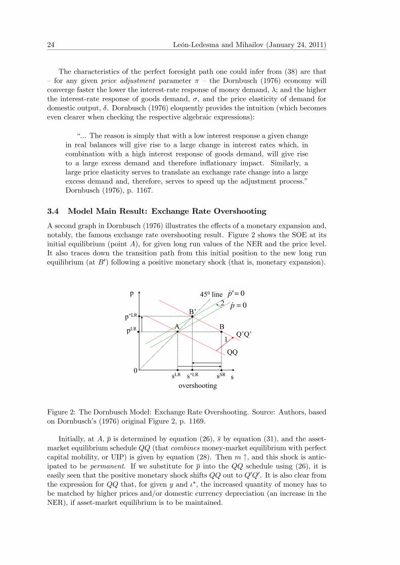
A second graph in Dornbusch (1976) illustrates the effects of a monetary expansion and,notably, the famous exchange rate overshooting result. Figure 2 shows the SOE at itsinitial equilibrium (point A), for given long run values of the NER and the price level.It also traces down the transition path from this initial position to the new long runequilibrium (at B0) following a positive monetary shock (that is, monetary expansion).

QQ

B’

AQ’Q’

450 linep

ssLR s’LR sSR

p’LR

pLR

0

B

1

2 0=p&0'=p&

overshooting

Figure 2: The Dornbusch Model: Exchange Rate Overshooting. Source: Authors, basedon Dornbusch’s (1976) original Figure 2, p. 1169.

Initially, at A, p is determined by equation (26), s by equation (31), and the asset-market equilibrium schedule QQ (that combines money-market equilibrium with perfectcapital mobility, or UIP) is given by equation (28). Then m ↑, and this shock is antic-ipated to be permanent. If we substitute for p into the QQ schedule using (26), it iseasily seen that the positive monetary shock shifts QQ out to Q0Q0. It is also clear fromthe expression for QQ that, for given y and ι∗, the increased quantity of money has tobe matched by higher prices and/or domestic currency depreciation (an increase in theNER), if asset-market equilibrium is to be maintained.


We now describe in greater detail the economic forces that lead to the exchange rateovershooting phenomenon.

1. At the initial level of prices p, the positive monetary shock, from (24), reducesdomestic (nominal) interest rates, that is, ι ↓. This is because y is assumedfixed and p is predetermined in the short run. This leads to an anticipation ofa domestic currency depreciation in the long run and, therefore, at the currentNER, to an expectation of a depreciating exchange rate. Both the falling interestrate and the expected depreciation reduce the attractiveness of domestic-currencydenominated assets, thus leading to incipient capital outflow and causing the spotrate to depreciate, s ↑. “. . . the extent of that depreciation has to be sufficient togive rise to an anticipation of appreciation at just sufficient a rate to offset thereduced domestic interest rate”, Dornbusch (1976), p. 1168. Hence, at point B,we have that s > s ⇔ s − s > 0 ⇔ expected appreciation. This first stage ofthe adjustment process of the SOE, only through the NER, corresponds to theconstant-price path from A to B, where the economy finds itself in a short-runequilibrium.

2. At point B, however, the lower interest rates and the lower relative price of do-mestic goods will cause domestic prices to start rising (there is excess demand fordomestic output). This gradually reduces real money balances, rising interest ratesand, thus, the currency depreciation reverses into an appreciation which continuesuntil the point where the spot NER reaches its new long run equilibrium. Thatis, from the (s− s) term of the QQ schedule (28), we get a process of a gradualupward adjustment of prices until the point when s− s = 0⇔ s = s. This secondstage of the SOE’s adjustment to a permanent monetary shock corresponds to asimultaneous adjustment of the NER and the price level until the new long-runequilibrium is reached at B0.

In effect, such a two-stage adjustment implies exchange rate overshooting, a phe-nomenon whereby the spot exchange rate temporarily exceeds its new long-run value,illustrated by the short-run equilibrium at point B in Figure 2.

To better understand overshooting, let us focus on some important features of theDornbusch (1976) model. Equation (30) says that the rate of inflation,

·p, is proportional

(via π) to excess demand for goods, lnD − lnY . As Mark (2001), p. 186, points out,because excess demand is always finite, the rate of change in goods prices is always finitetoo, so there are no jumps in the price level. If the price level cannot jump, then at anypoint in time it is instantaneously fixed. The adjustment of the price level toward itslong run value must occur over time, and it is in this sense that goods prices are stickyin the Dornbusch (1976) model.

Now bearing in mind that (i) p is instantaneously fixed because of the sticky-priceassumption, (ii) y is fixed too and (iii) ι∗ is constant and taken as given by the SOE,first totally differentiate equation (24). The result from the differentiation shows thatan unanticipated23 monetary expansion, dm > 0, will produce the liquidity effect, i.e.,dι < 0, of which there was mention before:

23As stressed by Mark (2001) in footnote 6 on p. 187, this often used thought experiment in economicanalysis brings up an uncomfortable question under the common assumption, as in Dornbusch (1976),of perfect foresigt: how then can a shock be unanticipated?


dι

dm= −1

λ< 0. (39)

Also, (iv) an increase in money causes an equiproportionate increase in prices andthe exchange rate in the long run (i.e., the long run homogeneity property that parallelsmoney neutrality we also mentioned earlier):

ds = dp = dm.

Then totally differentiate (22) using ds = dm (and holding ι∗ constant) in (23) toobtain:

dι = θ

⎛⎝ dm|z=ds

− ds

⎞⎠ .Use the above expression to eliminate dι in (39):

θ (dm− ds)

dm= −1

λ.

Finally solving for the instantaneous depreciation ds yields:

ds = dm+1

λθdm,

ds =

µ1 +

1

λθ

¶dm|z=ds

, (40)

and since

1 +1

λθ> 1,

we obtain

ds > ds,

which is the exchange-rate overshooting result derived analytically.24 The extentof this overshooting will depend, as clear from (40), on two parameters of the model,the interest-rate semi-elasticity in the money demand function, λ, and the expectations(formation) coefficient, θ. A high interest response of money demand (high λ) will serveto dampen the overshooting because it implies, from (24), that a given expansion inthe (real) quantity of money will only induce a small reduction in the interest rate.

24An alternative way to obtain the same result, which however misses the point about the liquidityeffect, is to totally differentiate directly equation (25):

dp|z=0

− dm = −φ dy|z=0

+ λ dι∗|z=0

+ λθ (ds− ds) ,

or

−dm = λθ (ds− ds)

and then use again the long run homogeneity assumption allowing us to replace ds = dm and finallysolve for ds

dm= 1 + 1

λθ.


The latter, from (22), requires only a small expectation of appreciation to offset it andtherefore, given θ and s, only a small depreciation of the spot rate s (in excess of thelong run NER) to generate that expectation. A similar interpretation applies to thecoefficient of expectations in equation (40), θ.

As Dornbusch (1976) points out, the short run effects of monetary expansion arethus entirely dominated by asset markets and, more specifically, by capital mobility andexpectations formation. This feature of his model corresponds to the crucial assumptionthat asset market prices such as the exchange rate adjust fast relative to the price ofdomestic output (the price level) in the goods market.

We can also observe that, from (40) the volatility of exchange rate changes is higherthan that of changes in fundamentals since V ar[ds] =

¡1 + 1

λθ

¢2V ar[dm]. This is one

of the prominent facts the model originally aimed to explain. A careful examination ofthe adjustment process to a monetary shock also shows that the model is compatiblewith the other stylised facts spelled out in Section 3.1.

4 Empirics of the Nominal Exchange Rate and the Ran-dom Walk Hypothesis

So far we have presented in detail two key theoretical models of exchange rate dynamics.A central issue in macroeconomics is how well these models fare when tested againstthe data. Important changes in the way researchers develop theory are due to empiricalfindings that lend support or stand against theory conclusions. Possibly nowhere elsein international macroeconomics is this interaction so important as in exchange ratedetermination theory. In this section, hence, we review how successful dynamic macroe-conomic models are in explaining the behavior of exchange rates. We focus here mainlyon the monetary model, but the results easily apply to other fundamentals-based mod-els. The evidence reviewed pertains mainly to the ability of structural macroeconomicmodels to forecast exchange rates, although this is not the only possible way of assessingtheory.25

4.1 Meese and Rogoff (1983): The Exchange Rate Disconnect Puzzle

There is a very large applied literature studying the power of key exchange rate modelsto forecast out-of-sample over horizons of up to four years. The literature started withMeese and Rogoff’s (1983 a, b) conclusion that a set of widely used structural (i.e.,theory-based) models, including the monetary model and the Dornbusch model, cannotpredict future exchange rates better than the simplest, but not very informative, timeseries model, the random walk. In a nutshell, the random walk without drift is a uni-variate time series model which implies that the best prediction for the future level ofa variable zt is its level today,26 i.e., Et [zt+1] = zt.27 In fact, what Meese and Rogoff

25Other possible criteria can be performance in-sample, the economic value of predictability for in-vestors (Abhyankar et al., 2005), ability to predict the direction of exchange rate changes and, moregenerally, economic value for policy makers. It also has to be noted that, following Clements and Hendry(2001), incorrect but simple models can outperform correct models in terms of forecast accuracy.26This also represents static expectations, as no change is anticipated. Recall also the discussion in

section 3.4. of Chapter 1 about unit-roots and mean-reversion.27Kilian (1999) favours comparison with a random walk model with drift, Et [zt+1] = υ + zt, so that

the model predicts a constant rate of change of zt equal to υ.


(1983) found was often termed the random walk hypothesis of the exchange rate. Itbasically means that the exchange rate appears to be (close to) a random walk process,hence difficult to predict by structural exchange rate models of the kind we studied inthis chapter. The hypothesis also forms part of the wider exchange rate disconnect puzzlein Obstfeld and Rogoff (2001): the very weak connection between the NER and virtu-ally any macroeconomic fundamentals.28 In a way, such a conclusion made senselessearlier and further attempts to try to explain exchange rate determination and dynam-ics by modelling macroeconomic details of relevance to the exchange rate. Some of theresearch on exchange rates that followed, therefore, directed its interest to purely sta-tistical modelling of exchange rates, e.g., the literature on the fundamental equilibriumexchange rate (FEER) or the behavioural equilibrium exchange rate (BEER).29 Otherresearchers began focusing on a deeper study of what became known as the microstruc-ture approach to the exchange rate, to which we shall return later in the book. Muchof the profession continued to be interested in improving the theoretical foundations ofexchange rate modelling, by incorporating additional and more realistic features intotraditional exchange rate macro-models, and notably by deriving equilibrium conditionsfrom microeconomic principles of agents’ optimisation, as we shall see in the next partsof the book.

Let us now provide more detail here on the persistent and widely debated empiricalfailure of structural exchange rate models.30 Meese and Rogoff (1983a) compared theforecasting performance of two types of exchange rate models: structural, such as themonetary or Dornbusch models, and time series models, such as the random walk modelor the unconstrained vector autoregression (VAR) we shall sketch further down. Theysummarised, in fact, three models, the third one an extension of the Dornbusch model toincorporate consideration of current account effects, into a general (semi-reduced form)specification:

s = a0+ a1 (m−m∗) + a2 (y − y∗) + a3 (ι− ι∗) + a4 (πe − πe∗) + a5tb+ a6tb

∗+ u. (41)

The notation in (41) is as introduced thus far, with the interest rates being short-term, expected inflation rates (πe, πe∗) long-run, and tb and tb∗ being cumulated tradebalances. The disturbance term u may be serially correlated. The Home variables areproxied by data for the US, while the Foreign variables (denoted by asterisk) correspondto data for Germany, the UK, Japan and a trade-weighted index, respectively. As onecan see, (41) expresses the exchange rate as a function of Home-Foreign differentials inmoney supplies, real incomes, interest rates, expected inflation rates and of the levelsof cumulative trade balances. The above general specification implies some constraints,nesting the three structural models employed in the Meese-Rogoff tests. For example,one assumption is that a1 = 1, which in a more formal language states that the exchangerate exhibits homogeneity of degree 1 in relative money supplies. Furthermore, Meeseand Rogoff (1983a) impose the constraints that the coefficients to the Home and Foreign

28The other manifestation being that transitions to floating-exchange-rate regimes lead to sharp in-creases in nominal and real exchange rate volatility with no corresponding changes in the volatility offundamentals.29See, e.g., Clark and MacDonald (1998) and Isard (2007).30We follow in our exposition the original papers, in particular Meese and Rogoff (1983 a, b), Mark

(1995), Rogoff (2001), Engel and West (2005), Engel, Mark and West (2007) and the comments to thelatter paper.


money demand functions and price adjustment equations are the same (which is not thecase, however, for the trade balances).31 Then, if a4 = a5 = a6 = 0, the generalspecification (41) reduces to the monetary model. The Dornbusch model, which impliesslow domestic price adjustment, can be obtained instead by setting a5 = a6 = 0, sincenow interest rate differentials do not cancel out immediately due to price stickiness.The third structural model Meese and Rogoff (1983a) test corresponds to the generalspecification itself, with no zero coefficients at all. The authors note that all thesethree regressions perform reasonably well in-sample. Yet out-of-sample they do notforecast better than a simple univariate random walk or an unconstrained multivariateVAR. The random walk is a first logical benchmark against which one would judgeabout any improvement of fit or forecasts arising from ‘enlightenment’ from economictheories because according to the random walk model no information could help predictfuture change. The random walk is, thus, agnostic, always forecasting no change.32

Furthermore, the simple random walk model requires no estimation, while the VARMeese and Rogoff (1983a) estimate is of the form:

st = a1st−1 + a2st−2 + ...+ anst−n +B01Xt−1 +B02Xt−2 + ...+B0nXt−n + ut,

where Xt−j is a vector of the explanatory variables in the single-equation regression(41), lagged j periods, the aj ’s are autoregressive coefficients, and Bj is a vector ofcoefficients.33 The other six univariate time series models, in addition to the randomwalk, that Meese and Rogoff (1983a) employed were simple autoregressive models withdifferent lag selection criteria available in the econometric literature at the time. Themodels were estimated using Ordinary Least Squares (OLS), Generalised Least Squares(GLS) to correct for residual autocorrelation of orders 1 and 5, and an Instrumental Vari-ables (IV) estimator that also corrects for residual autocorrelation.34 The forecastingperformance of all these models, structural and statistical, was compared along theirout-of-sample accuracy, the latter measured by three alternative but complementarystatistics, mean error (ME), mean absolute error (MAE) and root mean square error(RMSE), defined as follows:

ME ≡Nk−1Xq=0

F (t+ q + k)−A (t+ q + k)

Nk,

MAE ≡Nk−1Xq=0

|F (t+ q + k)−A (t+ q + k)|Nk

,

RMSE ≡vuutNk−1X

q=0

[F (t+ q + k)−A (t+ q + k)]2

Nk,

31Meese and Rogoff (1983a), p. 6, report that no gain in out-of-sample fit results from estimatingseparate coefficients for the Home and Foreign money supplies and real incomes.32Or a constant rate of change in the case of the random walk with drift.33 In fact, with monthly data Meese and Rogoff (1983a), p. 9 and footnote 9, have estimated the

uniform lag length across their seven equations in the VAR system to be 2 for all specifications of theForeign country, except for Japan, when this lag was 4.34They also use an estimator that minimises absolute deviations (MAD). This estimator is believed

to be more robust for series that display “fat tails” (and hence non-normality) as is the case with manyfinancial variables.


where k = 1, 3, 6, 12 is the forecast step, Nk the total number of forecasts in theprojection period for which A (t) is the actual value and F (t) the corresponding forecastvalue. The principal criterion applied for comparing the forecasts is RMSE. Yet RMSE isnot appropriate if exchange rates are governed by a non-normal stable Paretian processwith infinite variance, and here comes one rationale for adding MAE, the other beingthat MAE is also useful when the distribution has fat tails (known too as leptokurticdistributions and empirically common among asset prices). Meese and Rogoff’s (1983a)justification for adding ME as well is that by comparing MAE and ME they can ascertainwhether a model systematically over- or underpredicts. The main results are summarisedin Table 1, which is slightly adapted from the original study (p. 13) and reports onlythe RMSE.35

What is evident in the table is that none of the models achieves systematicallyand significantly lower RMSE than the random walk.36 Moreover, actual values of theexplanatory variables in the structural models were used to obtain the exchange rateforecasts instead of forecasts of these explanatory variables. Meese and Rogoff (1983a)claim that such a procedure actually favours structural models, an issue to which we willreturn later. Thus, the random walk emerges as the model that predicts the exchangerate no worse than either time series models or structural models. Hence, exchangerate dynamics appear to be better approximated by a random walk.

4.2 Explaining the Meese and Rogoff (1983) Results

The reaction to the Meese-Rogoff results has become a subdiscipline within interna-tional macroeconomics in itself. Exchange rate forecasting is not only a potentiallyuseful tool for investors seeking to gain returns from currency trading, but a way oftesting the validity of fundamentals-based models of exchange rate determination. It isnot surprising, hence, that the profession has greatly built up and developed on theseinitial results. Much of the debate has been enriched by advances in the econometrictheory of time series, which has formed the core of many responses to the random walkhypothesis. Recently, however, alternative explanations of the “puzzle” also focus onthe interpretation of well-established theory results. Here we review several of them ina succinct way.

4.2.1 Econometric Issues

As noted above, the way Meese and Rogoff obtain forecasts of exchange rates usingfundamentals is not a proper out-of-sample forecast, as they used the actual valuesof fundamentals instead of their forecasts. This led to the appearance of true out-of-sample forecast exercises, of which Mark (1995) is perhaps the best exponent. Hereports evidence that, at long-horizons, changes in the log of the exchange rate containa component that is significantly predictable by fundamentals.

This evidence of long-horizon predictability is based on the ideas coming from thetheory of integration and cointegration. As discussed in section 3.4 of Chapter 1, arandom walk is not mean reverting, meaning that its autoregressive root is equal to1. A time-series process like xt = xt−1 + t with t ∼ iid N(0, σt) is a non-stationaryprocess. Its variance grows with time and it can be shown that V ar(xt) = σ2t. That is,

35Meese and Rogoff also report forecasts from using forward rates to predict spot rates.36Meese and Rogoff (1983a), p. 12, described this result in stronger words, calling it ‘the striking

feature’ of the table.


Table 1: The Meese-Rogoff ResultsModel: Random Forward Univariate VAR Monetary Dornbusch Complete

walk rate AR model model eq. (41)Ex. rate Horizon

$/DM 1 3.72 3.20 3.51 5.40 3.17 3.65 3.506 8.17 9.03 12.40 11.83 9.64 12.03 9.9512 12.98 12.60 22.53 15.06 16.12 18.87 15.69

$/yen 1 3.68 3.72 4.46 7.76 4.11 4.40 4.206 11.58 11.93 22.04 18.90 13.38 13.94 11.9412 18.31 18.95 52.18 22.98 18.55 20.41 19.20

$/£ 1 2.56 2.67 2.79 5.56 2.82 2.90 3.036 6.45 7.23 7.27 12.97 8.90 8.88 9.0812 9.96 11.62 13.35 21.28 14.62 13.66 14.57

trade- 1 1.99 n.a. 2.72 4.10 2.40 2.50 2.74weighted 6 6.09 n.a. 6.82 8.91 7.07 6.49 7.11$ NEER 12 8.65 14.24 11.14 10.96 11.40 9.80 10.35

Source: Meese and Rogoff (1983), Table 1, p. 13, slightly shortened by theauthors. The table reports the RMSE for the full forecasting period, Novem-ber 1976 through June 1981, approximately in percentage terms. The threestructural models are estimated using and IV estimator to correct for first-order serial correlation. The measure of money is narrow money (M1-B) andthe long-term interest rate differential serves as the proxy for the long-runexpected inflation differential in the two sticky-price models.

it has infinite memory as it permanently accumulates shocks and hence diverges fromits initial value x0. A variable like xt can be transformed into a stationary variableby applying the first difference operator, so that ∆xt is a zero mean constant varianceprocess. This is usually termed an integrated process of order 1 and denoted I(1), ora difference stationary variable, since first differencing it will result in a stationary (orI(0)) process.

There is little doubt that many macroeconomic variables can be represented as I(1)processes.37 However, for any pair of I(1) variables, if there is any linear combinationof the two that yields a stationary process, then they are said to be cointegrated. Theidea of cointegration was first introduced by Granger (1981). Suppose that we observetwo I(1) variables xt and yt. Then xt and yt are cointegrated if there exists a β suchthat yt − βxt is I(0). This means that in the regression equation

yt = βxt + ut,

the error term ut is an I(0) process so that xt and yt do not drift away from each otherbut are tied together by a long-run relationship given by the cointegration vector (-1 β).

37See Aksoy and León-Ledesma (2008) for an analysis on a set of 249 macroeconomic variables for theG7 countries.


That is, even if the two variables are non-stationary, they share an equilibrium relation.Hence, by the Engle and Granger (1987) error-correction representation theorem eitheryt or xt has to adjust towards this long-run relationship. That is, in the long-run, current(time t) deviations from equilibrium must be corrected so that changes in the variablesfrom t to any t+k must be in the direction of this equilibrium relationship. This means,then, that ut should be a predictor for ∆xt,t+k or ∆yt,t+k.

If we go back to equation (14) in the monetary model, we can rearrange it so that

st − ft = λ (Et [st+1]− st) . (42)

The right-hand side of this equation can be solved by using the present-value (no-bubbles) solution for st (18), so that

λ (Et [st+1]− st) = λ

⎛⎝γkX

j=0

(1− γ)jEt [ft+1+j ]− γkX

j=0

(1− γ)jEt [ft+j ]

⎞⎠ =

= λγkX

j=0

(1− γ)jEt [∆ft+j+1] .

Hence, given that λγ = 1− γ, we obtain

st − ft =kX

j=1

(1− γ)jEt [∆ft+j ] . (43)

Both st and ft are commonly found to be non-stationary variables. But looking atequation (43), since ∆ft is stationary, the discounted sum of expected future changes inthe fundamentals must also be stationary.38 Hence, the theory suggests that st and ftare cointegrated. This means that st − ft should be a predictor for ∆st,t+k, and hencefundamentals could help forecast exchange rate returns, at least for long-horizons. Thisis tested by Mark (1995) using the following regression model:

st+k − st = β(st − ft) + εt+k, (44)

where εt+k is an error term, β an error-correction coefficient, k the forecast horizonand t = 1, 2, . . . , T . If fundamentals help explaining exchange rates, we would expect βto be positive, statistically significant, and an increasing function of k. This equation isused by Mark (1995) to compare the forecasts of a fundamentals-based model with thoseof a naïve random walk. The value for parameter φ for the construction of fundamentalscan be either estimated or pre-fixed to any value between 1 and 0.39 Then equation (44)can be estimated for a sub-sample [1, 2, . . . , τ ], with τ < T , and used to obtain out-of-sample k-step ahead forecasts. That is, forecasts from (44) for observations τ + 1, τ +2, . . . , τ + k. Then the equation is estimated up to observation τ + 1 and forecastsobtained for τ + 2, τ + 3, . . . , τ + k + 1. This process is recursively repeated until weobtain the last estimate up to observation T − k. This yields a series of forecasts for

38 If the fundamentals follow a driftless random walk ft = ft−1 + t, then ∆ft = t. Since t ∼iid N(0, σt), then

kPj=1

(1− γ)jEt [∆ft+j ] must also be a zero-mean stationary process.

39The results reported by Mark (1995) use a pre-fixed value of φ = 1.


each different horizon k. We can then compute the RMSE and compare it to that of arandom-walk. A simple, yet statistically not devoid of problems, metric for comparison isto calculate Theil’s statistic U = RMSEf/RMSERW , where RMSEf and RMSERW

are the RMSE of the fundamentals and the random walk models respectively. If thisratio is below unity, then fundamentals-based models outperform the random-walk atthat particular horizon. Mark (1995) performs forecasts using quarterly data for forecasthorizons of k = 1, 4, 8, 12, 16 and finds a significant forecastable exchange rate componentfor the Deutsche Mark, Japanese Yen and Swiss Franc against the US dollar, especiallyfor forecast horizons of 12 and 16 quarters. Mark and Sul (2001) use a panel versionof (44) by pooling data for 19 industrialised countries. They find that the monetarymodel outperforms the random-walk for 16 quarter horizons, but also for 1 quarter in asubstantial number of countries.

We reproduced Mark’s (1995) test for the quarterly bilateral exchange rates ofCanada, Japan and the UK against the US dollar for the period 1974:1 to 2001:3.We set t0 in 1987:3 so as to capture about half of the sample and forecast on the otherhalf. The results of Theil’s U index are reported in Table 2 for k = 1, 6, 12, 16, wherewe pre-fixed the value of φ to 1. We can observe that, for 1-quarter ahead forecasts, themodel only marginally outperforms the random walk (RW) for Japan, being practicallyindistinguishable from the RW for the other two. The forecast performance does notimprove for Canada. However, for Japan and the UK, it substantially outperforms theRW for the 16 quarters forecast. These results support the evidence in Mark (1995) thatfundamentals can improve on a RW when forecasting exchange rates at long-horizons.

Table 2: Long-Horizon ForecastsCountry Canada Japan UKHorizon1 0.998 0.981 1.0006 1.014 0.955 0.97612 1.033 0.939 0.93816 1.009 0.847 0.889

Source: Authors’ own calculations of Theil’s U =

RMSEf/RMSERW . Money is M1 and output is GDP.Data from IMF’s IFS database for 1974:1—2001:3.

The assumption of the literature is that Meese and Rogoff (1983) give an “unfair”advantage to the fundamentals model since they use true values of the fundamentals,rather than their forecasts. Engel, Mark and West (2007) challenge this assumption byarguing that the in-sample fit of the model can be arbitrarily changed by the way wewrite the model. One can re-scale the variables in such a way that they yield a smallervariance, a problem that is not present in (44). They also claim that, if exchange ratesare also driven by “unobserved” fundamentals, the use of actual observed values mayworsen forecasts if these are correlated with the “unobserved” variables.

The recent literature has focused on improving the forecast performance of modelslike (44) by focusing on a variety of econometric problems. These range from the use ofhistorical data (Rapach and Wohar, 2002), panel data (Mark and Sul, 2001 and Groen,2005), high-persistence (Rossi, 2005), parameter instability (Rossi, 2006), small-sampleinference (Kilian, 1999), nonlinear mean-reversion in deviations from fundamentals (Kil-ian and Taylor, 2003), etc. The findings of these studies all point towards statistically


and economically significant gains from using fundamentals to forecast exchange rates.However, this appears to happen only at long-horizons, and this positive performanceis not robust.40

4.2.2 Engel and West (2005): The Exchange Rate as a Near-Random Walk

In an important paper, Engel and West (2005) take a different route. They claim thatexchange rates and fundamentals are linked in a way that is broadly consistent withasset-pricing models of the exchange rate. Looking back at equation (18), one caneasily see that the exchange rate should be a good predictor of the future evolution offundamentals, as they reflect market participants’ expectations about the future streamof fundamentals. In order to test this hypothesis, they present Granger-causality testsbetween fundamentals and exchange rates for the G7 countries and for different measuresof fundamentals. The concept of Granger-causality simply means that, for two stochasticvariables xt and yt, yt Granger-causes xt if past values of yt improve the forecasts of xtbeyond the information contained in past values of xt. We have already seen that, iftwo variables are cointegrated, then at least one of them adjusts towards the long-runrelationship implying Granger-causality. But if two I(1) variables are not cointegrated,there may still be information content if we model them in first-differences. Engel andWest (2005) find little evidence in favour of cointegration between exchange rates andfundamentals, and hence run Granger-causality tests in first differences by estimating:

∆ft =dX

i=1

ζi∆ft−i +dX

i=1

ξi∆st−i + εt, (45)

where d is the maximum lag-length that can be determined by a variety of methods.The Granger-causality test then consists of a joint test of significance for the ξi coeffi-cients (using an F -test or a Likelihood Ratio (LR) test).41 They perform the test forboth variables, that is, Granger-causality from ∆st to ∆ft and from ∆ft to ∆st. Theyfind that exchange rates help predict fundamentals for a number of cases, but confirmthat fundamentals are of little use in predicting the exchange rate. This is then stillcompatible with the asset approach to exchange rates.

The question is, however, why can’t fundamentals predict exchange rates? This isexplained by an analytical finding that, under plausible conditions, models like (18)actually predict that the exchange rate will behave as a near -random walk. This is thecase if the discount factor 1− γ approaches unity and fundamentals are I(1) processes.Under these conditions, they prove that the log of the exchange rate approximates aprocess which, for finite samples, is practically undistinguishable from the random walk.It is not surprising, hence, that the NER appears to be well approximated by a randomwalk.

Engel, Mark and West (2007) claim that this theorem renders forecast comparisonsrelative to the random walk unreliable.42 So they propose a number of alternative ways

40See Cheung, Chinn and García-Pascual (2005) for a general assessment. Rogoff and Stavrakeva(2008) also show that exchange rate forecasts are not robust to the choice of forecasting window (essen-tially the choice of τ).41Properly speaking, this is a test for Granger non-causality, i.e. the null hypothesis is non-causality.42Sarno and Sojli (2009) directly test the implications of the model by estimating the discount factor

using survey data on expectations. They find point estimates in the range of 0.98-0.99, which supportsthe Engel and West (2005) hypothesis.


of model evaluation, including in-sample fit, the role of monetary policy in affectingexpectations, the response by exchange rates to news about future fundamentals, modelsthat account for observed exchange rate volatility as well as models that allow for surveyforecasts in determining the future value of the fundamentals. Their conclusions are lesspessimistic than the prevailing literature, claiming that fundamentals-based models,when analyzed from different angles, are not as bad as previously thought.43

4.2.3 Where Do We Stand?

The large empirical literature on the link between fundamentals and exchange rates,despite having started with rather nihilistic results, has proven useful in understandingthe dynamics of exchange rates. Several facts have been accumulating since the seminalwork of Meese and Rogoff. Without attempting to be exhaustive, some of these factscan be summarized in the following points:

• Exchange rate models appear to beat the random walk at forecast horizons beyondone year, although these results are not fully robust and shorter horizon forecastsstill remain problematic.

• The in-sample fit of exchange rate models is satisfactory although, as Engel, Markand West (2007) maintain, is not a reliable benchmark.

• As stated by Rogoff (2001a), in periods of current and/or expected high inflation(especially for emerging markets) exchange rate models have proven extremelyuseful.

• Exchange rates and fundamentals appear to be linked in a way that is not in-compatible with asset-price models. Specifically, exchange rates seem to containsignificant information about the future evolution of fundamentals; a relation thatRossi (2007) finds to be quite robust.

• Fundamentals are good predictors of exchange rates for so-called “commodity cur-rencies” pertaining to the Australian, Canadian, and New Zealand dollars (Chenand Rogoff, 2003). Because a significant share of the overall exports of each ofthese three countries is accounted for by commodities, the respective country’smajor commodity export prices are highly correlated with exchange rate changeseven in out-of-sample forecasts.

• There is ample evidence that news about macroeconomic fundamentals affect ex-change rates in a manner that is compatible with theoretical predictions.

The important question is then to analyze the potential reasons for the failure ofthese models beyond mere statistical issues. Rogoff (2001a and 2001b) summarisedthe reasons for this failure. One cause for the failure is the link between exchangerates and prices, which leads to the famous PPP condition: this link is a very long runrelationship, as claimed in Rogoff (1996) too, with the half-life of PPP deviations beingvery persistent (3 to 4 years) in linear models. A second cause is the potential instabilityof the money demand function, which would make the link between money and pricesless transparent. This adds to the well-reported changes in monetary policy stance in

43See Rogoff ’s (2007) reply to Engel, Mark and West (2007) for further discussion of these points.


most major industrialised countries: the current practice is to set interest rates, makingmoney supply endogenous.44 A related point is that this change in policy stance led toa downward convergence process in inflation rates across major countries, making theeffects of changes in monetary aggregates more difficult to detect. A final, perhaps morefundamental, cause has to do with the magnitude of market segmentation: even acrossindustrialised countries, it is of an order consistent with international transactions costsfor all GDP (not just the actually traded goods) averaging 25% or more, an argumentemphasised by Obstfeld and Rogoff (2001).

In light of these points, and given the simplifying assumptions of standard theoreticalmodels, one could indeed claim that they perform well empirically in spite of theirsimplicity. As a conclusion, Rogoff (2007) writes that “exchange rates remain a verytough nut to crack, even after the Great Moderation in macroeconomic variables. Rightnow, things still look pretty good if we can call the glass ten percent full.”

Problems and Exercises

1. Government spending in the overshooting model. Assume that we now introducegovernment spending (G or lnG = g) in the model. The expression for aggregatedemand (29) now becomes

lnD = u+ δ (s− p) + γy − σι+ g,

Analyse the impact on the exchange rate of an expansionary fiscal policy, dg.Would this fiscal policy expansion induce NER overshooting?

2. Dornbusch (1976) Part V. In the sticky price model, suppose that we relax theassumption of fixed output and we allow short run changes in output to respond tochanges in aggregate demand. The goods-market equilibrium condition becomes

y = lnD ≡ u+ δ (s− p) + γy − σι,

which can also be written as

y = μ [u+ δ (s− p)− σι] , μ ≡ 1

1− γ> 0,

and the price adjustment equation is now

·p = π (y − y) ,

where y denotes the full-employment level of output, so that inflation is now afunction of the output gap. Find the equilibrium of the model and analyse the im-pact of a permanent unanticipated monetary expansion. Is there an overshootingeffect?

3. Forecasting exchange rates. Using the long run forecasting equation (44) andassuming values for λ = [0.1, 0.4, 1.0], compute the 1, 2, 4, 8 and 16 quartersahead forecast for the bilateral NER of Canada, Japan and the UK against theUSD. Use the data provided in www.oup.co.uk/leonledesma-mihailov/Ch3.45

44Engel, Mark and West (2007) discuss this point at length and provide further references.45A Gauss 8.0 code is provided in the webpage.


References

[1] Abhyankar, Abhay, Lucio Sarno and Giorgio Valente (2005), “Exchange Rates andFundamentals: Evidence on the Economic Value of Predictability”, Journal of In-ternational Economics 66, 325-348.

[2] Akerlof, George A. and Janet L. Yelen (1985), “A Near-Rational Model of theBusiness Cycle, with Wage and Price Inertia”, Quarterly Journal of Economics100 (Supplement), 823-838.

[3] Aksoy, Yunus and Miguel A. León-Ledesma (2008) “Non-Linearities and Unit Rootsin G7 Macroeconomic Variables,” The B.E. Journal of Macroeconomics 8 (Topics),Article 5.

[4] Baxter, Marianne and Alan C. Stockman (1989), “Business Cycles and the Ex-change Rate Regime: Some International Evidence”, Journal of Monetary Eco-nomics 23, 377-400.

[5] Black, Stanley W. (1973), “International Money Markets and Flexible ExchangeRates”, Princeton Studies in International Finance No. 32, Princeton, NJ: Prince-ton University Press.

[6] Branson, William and Wilhem Buiter (1983), “Monetary and Fiscal Policy andFlexible Exchange Rates”, chapter 9 in Bhandari, J. S. and Putnam, B. H. (eds.),Inflation and Employment in Open Economies, Amsterdam: North Holland.

[7] Branson, William and Dale Henderson (1985), “The Specification and Influence ofAsset Markets”, chapter 15 in Jones, R. W. and Kenen, P. B. (eds.), Handbook ofInternational Economics, Vol. II, Amsterdam: North Holland.

[8] Cagan, Phillip (1956), “The Monetary Dynamics of Hyperinflation”, in Friedman,M. (ed.), Studies in the Quantity Theory of Money, Chicago: University of ChicagoPress.

[9] Cassel, Gustav (1918), “Abnormal Deviations in International Exchanges”, Eco-nomic Journal 28, 413-415.

[10] Cassel, Gustav (1921), The World’s Monetary Problems, London: Constable.

[11] Chen, Yu-chin and Kenneth Rogoff (2003), “Commodity Currencies”, Journal ofInternational Economics 60 (May), 133-160.

[12] Cheysson, Emile (1887), “La statistique géométrique : ses applications industrielleset commerciales”, Le Genie civil, Jan. 29 and Feb. 5, 10, 206-210 and 224-228.

[13] Cheung, Yin-Wong, Menzie D. Chinn and Antonio Garcia-Pascual (2005), “Empir-ical Exchange Rate Models of the Nineties: Are Any Fit to Survive?” Journal ofInternational Money and Finance 24, 1150-1175.

[14] Clark, Peter and Ronald MacDonald (1998), “Exchange Rates and Economic Fun-damentals: A Methodological Comparison of BEERs and FEERs”, IMF WorkingPaper WP/98/67.


[15] Clements, Mike P. and David F. Hendry (2001), “Forecasting With Difference andTrend Stationary Models”. The Econometrics Journal 4, S1-S19.

[16] Dornbusch, Rudiger (1976), “Expectations and Exchange Rate Dynamics”, Journalof Political Economy 84 (6, December), 1161-1176.

[17] Engle, Robert and Clive W.J. Granger (1987) “Co-integration and Error-Correction: Representation, Estimation, and Testing,” Econometrica 55, 251-76.

[18] Engel, Charles and Kenneth D. West (2005), “Exchange Rate and Fundamentals”,Journal of Political Economy 84, 485-517.

[19] Engel, Charles, Nelson Mark and Kenneth D. West (2007), “Exchange Rate ModelsAre Not As Bad As You Think”, NBER Macroeconomics Annual 22, 381-441

[20] Evans, George W. (1985), “Expectational Stability and the Multiple EquilibriaProblem in Linear Rational Expectations Models”, Quarterly Journal of Economics100, 1217-1233.

[21] Evans, George W. (1991), “Pitfalls in Testing for Explosive Bubbles in AssetPrices”, American Economic Review 81, 922:930.

[22] Evans, George W. and Seppo Honkapohja (1995), “Adaptive Learning and Expec-tational Stability”, in Kirman, A. and Salmon, M. (eds.), Learning and Rationalityin Economics, Basil Blackwell: Oxford, 102-126.

[23] Evans, George W. and Seppo Honkapohja (2001), Learning and Expectations inMacroeconomics, Princeton and Oxford: Princeton University Press.

[24] Frankel, Jeffrey (1983), “Monetary and Portfolio Models of Exchange Rate Deter-mination”, in Bhandari, J. S. and Putnam, B. H. (eds.), Economic Interdependenceand Flexible Exchange Rates, Cambridge (Mass.): MIT Press, 84-115.

[25] Frenkel, Jacob A. (1976), “A Monetary Approach to the Exchange Rate: DoctrinalAspects and Empirical Evidence”, Scandinavian Journal of Economics 78 (2, May),200-224.

[26] Frenkel, Jacob A. and Harry G. Johnson (1976), The Monetary Approach to theBalance of Payments, London: Allen & Unwin.

[27] Gandolfo, Giancarlo (2001), International Finance and Open-Economy Macroeco-nomics, Springer.

[28] Granger, Clive W.J. (1981), “Some Properties of Time Series Data and Their Usein Econometric Model Specification”, Journal of Econometrics 16, 121-130.

[29] Groen, Jan J.J. (2005), “Exchange Rate Predictability and Monetary Fundamentalsin a Small Multi-Country Panel”, Journal of Money, Credit and Banking 37, 495-516.

[30] Hall, Stephen G., Zacharias Psaradakis and Martin Sola (1999), “Detecting Pe-riodically Collapsing Bubbles: A Markov-Switching Unit Root Test”, Journal ofApplied Econometrics 14, 143-154.


[31] Huang, Roger D. (1981), “The Monetary Approach to Exchange Rate in a EfficientForeign Exchange Market: Tests Based on Volatility”, Journal of Finance 36, 31-41.

[32] Hume, David (1752), “Of the Balance of Trade”, in Hume, D., Political Dis-courses, Edinburgh; reprinted in Hume, D. (1955), Writings on Economics, editedby Rotwein, E., London: Nelson, 60ff.

[33] Isard, Peter (2007), “Equilibrium Exchange Rates: Assessment Methodologies”,IMF Working Paper 07/296.

[34] Johnson, Harry G. (1977), “The Monetary Approach to the Balance of Payments”.Journal of International Economics 7, pp. 251-268.

[35] Keynes, John Maynard (1936), The General Theory of Employment, Interest andMoney, London: Macmillan.

[36] Killian, Lutz (1999), “Exchange Rates And Monetary Fundamentals: What DoWe Learn From Long-Horizon Regressions?,” Journal of Applied Econometrics 14,491-510.

[37] Killian, Lutz and Mark P. Taylor (2003) “Why Is It so Difficult to Beat the RandomWalk Forecast of Exchange Rates?,” Journal of International Economics 60, 85-107.

[38] Lindbeck, Assar (1976), “Approaches to Exchange Rate Analysis — An Introduc-tion”, Scandinavian Journal of Economics 78 (2, May), 133-145.

[39] Lucas, Jr., Robert E. (1972), “Expectations and the Neutrality of Money”, Journalof Economic Theory 4, 103-124.

[40] Mankiw, N. Gregory (1985), “Small Menu Costs and Large Business Cycles: AMacroeconomic Model of Monopoly”, Quarterly Journal of Economics 100 (May),529-539.

[41] Mark, Nelson (1995), “Exchange Rates and Fundamentals: Evidence on Long-Horizon Predictability”, American Economic Review 85 (1, March), 201—218.

[42] Mark, Nelson (2001), International Macroeconomics and Finance: Theory andEconometric Methods, Blackwell.

[43] Mark, Nelson and Donggyu Sul (2001), “Nominal Exchange Rates and MonetaryFundamentals: Evidence from a Small Post-Bretton Woods Panel”, Journal ofInternational Economics 53, 29—52.

[44] Markowitz, Harry (1952), “Portfolio Selection”, Journal of Finance 7 (March), 77-91.

[45] Meese, Richard C. and Kenneth Rogoff (1983a), “Empirical Exchange Rate Modelsof the Seventies: Do They Fit Out of Sample?”, Journal of International Economics14, 3-24.

[46] Meese, Richard C. and Kenneth Rogoff (1983b), “The Out-Of-Sample Failure ofEmpirical Exchange Rate Models: Sampling Error or Misspecification?”, in Frenkel,J. A. (ed.), Exchange Rates and International Macroeconomics, NBER and Univer-sity of Chicago Press.


[47] Mussa, Michael (1976), “The Exchange Rate, the Balance of Payments, and Mon-etary and Fiscal Policy Under a Regime of Controlled Floating”, ScandinavianJournal of Economics 78 (2, May), 229—248.

[48] Muth, John (1961), “Rational Expectations and the Theory of Price Movements”,Econometrica 29 (3, July), 315-335.

[49] Obstfeld, Maurice and Kenneth Rogoff (1996), Foundations of InternationalMacroeconomics, MIT Press.

[50] Obstfeld, Maurice and Kenneth Rogoff (2001), “The Six Major Puzzles in Interna-tional Macroeconomics: Is There a Common Cause?”, in Bernanke, B. and Rogoff,K. (eds.), NBER Macroeconomics Annual 2001, Cambridge: MIT Press, 339-390.

[51] Obstfeld, Maurice and Kenneth Rogoff (2003), “Risk and Exchange Rates”, inHelpman, E. and Sadka, E. (eds.), Economic Policy in the International Economy:Essays in Honor of Assaf Razin Cambridge: Cambridge University Press.

[52] O’Connell, J. (1984), “Stock Adjustment and the Balance of Payments”, EconomicNotes 1, 136-144.

[53] Psaradakis, Zacharias, Martin Sola and Fabio Spagnolo (2001), “A Simple Proce-dure for Detecting Periodically Collapsing Rational Bubbles”, Economics Letters72, 317-323.

[54] Rapach, David E. and Mark E. Wohar (2002) “Testing the Monetary Model ofExchange Rate Determination: New Evidence from a Century of Data”, Journal ofInternational Economics 58, 359-385.

[55] Ricardo, David (1821), Principles of Political Economy and Taxation, edited by E.C. Connor, G. Bell and Sons: London, 1911.

[56] Rogoff, Kenneth (1996), “The Purchasing Power Parity Puzzle,” Journal of Eco-nomic Literature 34, 647-68.

[57] Rogoff, Kenneth (2001a), “Monetary Models of the Dollar/Yen/Euro Nominal Ex-change Rate: Dear or Undead?” Economic Journal 109, F655-F659.

[58] Rogoff, Kenneth (2001b), “The Failure of Empirical Exchange Rate Models: NoLonger New, But Still True,” Economic Policy Web Essay (September).

[59] Rogoff, Kenneth (2002), “Dornbusch’s Overshooting Model After 25 Years: IMFMundell-Fleming Lecture,” IMF Staff Papers 49 (Special Issue), 1-35 (includingremarks by Rudiger Dornbusch).

[60] Rogoff, Kenneth (2007), “Comment on ’Exchange Rate Models Are Not as Bad asYou Think’,” NBER Macroeconomics Annual 22.

[61] Rogoff, Kenneth and Vania Stavrakeva (2008), “The Continuing Puzzle of ShortHorizon Exchange Rate Forecasting,” mimeo, Harvard University.

[62] Rossi, Barbara (2005), “Testing Long-Horizon Predictive Ability with High Persis-tence, and the Meese-Rogoff Puzzle”, International Economic Review 46, 61-92.


[63] Rossi, Barbara (2006), “Are Exchange Rates Really Random Walks? Some Evi-dence Robust to Parameter Instability”, Macroeconomic Dynamics 10, 20-38.

[64] Rossi, Barbara (2007), “Comment on ’Exchange Rate Models Are Not as Bad asYou Think’,” NBER Macroeconomics Annual 22.

[65] Samuelson, Paul A. (1964), “Theoretical Notes on Trade Problems”, Review ofEconomics and Statistics 46, 145-154.

[66] Sargent, Thomas (1973), “Rational Expectations, the Real Rate of Interest andthe Natural Rate of Unemployment”, Brookings Papers on Economic Activity 2,429-472.

[67] Sarno, Lucio and Mark Taylor (2002), The Economics of Exchange Rates, Cam-bridge University Press.

[68] Sarno, Lucio and Elvira Sojli (2009), “The Feeble Link Between Exchange Ratesand Fundamentals: CanWe Blame the Discount Factor?,” Journal of Money, Creditand Banking, forthcoming.

[69] Shiller, Robert J., (1981) “Do Stock Prices Move by Two Much to be Justified bySubsequent Changes in Dividends?” American Economic Review 71, 421-436.

[70] Thornton, Henry (1802), An Enquiry into the Nature and Effects of the Paper Creditof Great Britain, published in 1939 by Allen and Unwin: London.

[71] Tobin, James (1952), “Asset Holdings and Spending Decisions”, American Eco-nomic Review 42 (May), 109-123.

[72] Wheatley, J. (1803), Remarks on Currency and Commerce, Burton: London.

Indexadaptive expectations, 1, 3

bubble, 13bubbles, 12, 14, 15, 32

cointegration, 30, 31, 34

difference equation, 11, 13, 14

error-correction, 32exchange rate disconnect puzzle, 28

fundamentals, 10—15, 27, 28, 30, 32—35

Granger-causality, 34

integrated process, 31

logarithmic expansion, 7

monetary approach, 1, 6—10monetary model, 4—6, 9—12, 17, 19, 27,

29, 32, 33money demand, 7—10, 12, 17—19, 21, 24,

26, 29, 35Mundell-Fleming, 1, 9, 15

out-of-sample forecast, 30, 35overshooting, 1, 12, 15, 17, 24—26, 36

perfect foresight, 5, 17perfect foresigt, 4, 5, 15, 16, 23—25price-specie-flow mechanism, 6purchasing power parity (PPP), 6—8, 10,

35

quantity theory, 6

random walk, 1, 27—30, 32—35rational bubble, 13, 14rational expectations, 1, 3, 4, 14—16, 23

static expectations, 1sticky prices, 5, 15, 23stock approach, 4, 5

transversality condition, 12—14

Uncovered Interest Parity (UIP), 7—10,17, 18, 22, 24

vector autoregression, 28

42

Advanced International Macroeconomics and Finance OUP Book, Chapter … · 2014-04-01 · Advanced...

Documents

Transcript of Advanced International Macroeconomics and Finance OUP Book, Chapter … · 2014-04-01 · Advanced...