Advanced Integration Techniques - WordPress.comAdvanced Integration Techniques Advanced approaches...

Advanced IntegrationTechniques

Advanced approaches for solving many complex integrals using special functions and some

transformations

Second Version

ZAID ALYAFEAIYEMEN

mailto:[email protected]


Contents

1 Differentiation under the integral sign 10

1.1 Example . . . . . . . . . . . . . . . . . . . . . . . . . . . . . . . . . . . . . . . . . . . . . . . . . . . 10

1.2 Example . . . . . . . . . . . . . . . . . . . . . . . . . . . . . . . . . . . . . . . . . . . . . . . . . . . 11

1.3 Example . . . . . . . . . . . . . . . . . . . . . . . . . . . . . . . . . . . . . . . . . . . . . . . . . . . 12

2 Laplace Transform 14

2.1 Basic Introduction . . . . . . . . . . . . . . . . . . . . . . . . . . . . . . . . . . . . . . . . . . . . . 14

2.1.1 Example . . . . . . . . . . . . . . . . . . . . . . . . . . . . . . . . . . . . . . . . . . . . . . . 14

2.2 Example . . . . . . . . . . . . . . . . . . . . . . . . . . . . . . . . . . . . . . . . . . . . . . . . . . . 15

2.3 Convolution . . . . . . . . . . . . . . . . . . . . . . . . . . . . . . . . . . . . . . . . . . . . . . . . . 15

2.4 Inverse Laplace transform . . . . . . . . . . . . . . . . . . . . . . . . . . . . . . . . . . . . . . . . 15

2.4.1 Example . . . . . . . . . . . . . . . . . . . . . . . . . . . . . . . . . . . . . . . . . . . . . . . 15

2.5 Interesting results . . . . . . . . . . . . . . . . . . . . . . . . . . . . . . . . . . . . . . . . . . . . . 16

2.5.1 Example . . . . . . . . . . . . . . . . . . . . . . . . . . . . . . . . . . . . . . . . . . . . . . . 16

2.5.2 Example . . . . . . . . . . . . . . . . . . . . . . . . . . . . . . . . . . . . . . . . . . . . . . . 17

2.5.3 Example . . . . . . . . . . . . . . . . . . . . . . . . . . . . . . . . . . . . . . . . . . . . . . . 18

3 Gamma Function 19

3.1 Definition . . . . . . . . . . . . . . . . . . . . . . . . . . . . . . . . . . . . . . . . . . . . . . . . . . . 19

3.2 Example . . . . . . . . . . . . . . . . . . . . . . . . . . . . . . . . . . . . . . . . . . . . . . . . . . . 19

3.3 Example . . . . . . . . . . . . . . . . . . . . . . . . . . . . . . . . . . . . . . . . . . . . . . . . . . . 20

3.4 Exercises . . . . . . . . . . . . . . . . . . . . . . . . . . . . . . . . . . . . . . . . . . . . . . . . . . . 20

3.5 Extension . . . . . . . . . . . . . . . . . . . . . . . . . . . . . . . . . . . . . . . . . . . . . . . . . . . 21

3.5.1 Theorem . . . . . . . . . . . . . . . . . . . . . . . . . . . . . . . . . . . . . . . . . . . . . . . 21

3.5.2 Reduction formula . . . . . . . . . . . . . . . . . . . . . . . . . . . . . . . . . . . . . . . . 21

3.6 Other Representations . . . . . . . . . . . . . . . . . . . . . . . . . . . . . . . . . . . . . . . . . . . 21

3.6.1 Euler Representation . . . . . . . . . . . . . . . . . . . . . . . . . . . . . . . . . . . . . . . 21

3.6.2 Example . . . . . . . . . . . . . . . . . . . . . . . . . . . . . . . . . . . . . . . . . . . . . . . 23

3.6.3 Weierstrass Representation . . . . . . . . . . . . . . . . . . . . . . . . . . . . . . . . . . . 23

3.7 Laurent expansion . . . . . . . . . . . . . . . . . . . . . . . . . . . . . . . . . . . . . . . . . . . . . 24

3.8 Example . . . . . . . . . . . . . . . . . . . . . . . . . . . . . . . . . . . . . . . . . . . . . . . . . . . 25

3.9 More values . . . . . . . . . . . . . . . . . . . . . . . . . . . . . . . . . . . . . . . . . . . . . . . . . 26

1

3.10 Legendre Duplication Formula . . . . . . . . . . . . . . . . . . . . . . . . . . . . . . . . . . . . . 28

3.11 Example . . . . . . . . . . . . . . . . . . . . . . . . . . . . . . . . . . . . . . . . . . . . . . . . . . . 28

3.12 Euler’s Reflection Formula . . . . . . . . . . . . . . . . . . . . . . . . . . . . . . . . . . . . . . . . 29

3.13 Example . . . . . . . . . . . . . . . . . . . . . . . . . . . . . . . . . . . . . . . . . . . . . . . . . . . 30

3.14 Example . . . . . . . . . . . . . . . . . . . . . . . . . . . . . . . . . . . . . . . . . . . . . . . . . . . 31

4 Beta Function 33

4.1 Representations . . . . . . . . . . . . . . . . . . . . . . . . . . . . . . . . . . . . . . . . . . . . . . . 33

4.1.1 First integral formula . . . . . . . . . . . . . . . . . . . . . . . . . . . . . . . . . . . . . . . 33

4.1.2 Second integral formula . . . . . . . . . . . . . . . . . . . . . . . . . . . . . . . . . . . . . 33

4.1.3 Geometric representation . . . . . . . . . . . . . . . . . . . . . . . . . . . . . . . . . . . . 33

4.2 Example . . . . . . . . . . . . . . . . . . . . . . . . . . . . . . . . . . . . . . . . . . . . . . . . . . . 33

4.3 Example . . . . . . . . . . . . . . . . . . . . . . . . . . . . . . . . . . . . . . . . . . . . . . . . . . . 34

4.4 Example . . . . . . . . . . . . . . . . . . . . . . . . . . . . . . . . . . . . . . . . . . . . . . . . . . . 34

4.5 Example . . . . . . . . . . . . . . . . . . . . . . . . . . . . . . . . . . . . . . . . . . . . . . . . . . . 35

4.6 Example . . . . . . . . . . . . . . . . . . . . . . . . . . . . . . . . . . . . . . . . . . . . . . . . . . . 36

4.7 Example . . . . . . . . . . . . . . . . . . . . . . . . . . . . . . . . . . . . . . . . . . . . . . . . . . . 37

4.8 Example . . . . . . . . . . . . . . . . . . . . . . . . . . . . . . . . . . . . . . . . . . . . . . . . . . . 37

4.9 Example . . . . . . . . . . . . . . . . . . . . . . . . . . . . . . . . . . . . . . . . . . . . . . . . . . . 38

4.10 Exercise . . . . . . . . . . . . . . . . . . . . . . . . . . . . . . . . . . . . . . . . . . . . . . . . . . . . 38

5 Digamma function 39

5.1 Definition . . . . . . . . . . . . . . . . . . . . . . . . . . . . . . . . . . . . . . . . . . . . . . . . . . . 39

5.2 Example . . . . . . . . . . . . . . . . . . . . . . . . . . . . . . . . . . . . . . . . . . . . . . . . . . . 39

5.3 Difference formulas . . . . . . . . . . . . . . . . . . . . . . . . . . . . . . . . . . . . . . . . . . . . 39

5.3.1 First difference formula . . . . . . . . . . . . . . . . . . . . . . . . . . . . . . . . . . . . . 39

5.3.2 Second difference formula . . . . . . . . . . . . . . . . . . . . . . . . . . . . . . . . . . . . 40

5.4 Example . . . . . . . . . . . . . . . . . . . . . . . . . . . . . . . . . . . . . . . . . . . . . . . . . . . 40

5.5 Series Representation . . . . . . . . . . . . . . . . . . . . . . . . . . . . . . . . . . . . . . . . . . . 41

5.6 Some Values . . . . . . . . . . . . . . . . . . . . . . . . . . . . . . . . . . . . . . . . . . . . . . . . . 42

5.7 Example . . . . . . . . . . . . . . . . . . . . . . . . . . . . . . . . . . . . . . . . . . . . . . . . . . . 43

5.8 Integral representations . . . . . . . . . . . . . . . . . . . . . . . . . . . . . . . . . . . . . . . . . . 43

5.8.1 First Integral representation . . . . . . . . . . . . . . . . . . . . . . . . . . . . . . . . . . . 43

5.8.2 Second Integral representation . . . . . . . . . . . . . . . . . . . . . . . . . . . . . . . . . 45

2

5.8.3 Third Integral representation . . . . . . . . . . . . . . . . . . . . . . . . . . . . . . . . . . 45

5.8.4 Fourth Integral representation . . . . . . . . . . . . . . . . . . . . . . . . . . . . . . . . . 46

5.9 Gauss Digamma theorem . . . . . . . . . . . . . . . . . . . . . . . . . . . . . . . . . . . . . . . . . 47

5.10 More results . . . . . . . . . . . . . . . . . . . . . . . . . . . . . . . . . . . . . . . . . . . . . . . . . 47

5.11 Example . . . . . . . . . . . . . . . . . . . . . . . . . . . . . . . . . . . . . . . . . . . . . . . . . . . 48

5.12 Example . . . . . . . . . . . . . . . . . . . . . . . . . . . . . . . . . . . . . . . . . . . . . . . . . . . 48

5.13 Example . . . . . . . . . . . . . . . . . . . . . . . . . . . . . . . . . . . . . . . . . . . . . . . . . . . 50

5.14 Example . . . . . . . . . . . . . . . . . . . . . . . . . . . . . . . . . . . . . . . . . . . . . . . . . . . 51

5.15 Example . . . . . . . . . . . . . . . . . . . . . . . . . . . . . . . . . . . . . . . . . . . . . . . . . . . 52

6 Zeta function 54

6.1 Definition . . . . . . . . . . . . . . . . . . . . . . . . . . . . . . . . . . . . . . . . . . . . . . . . . . . 54

6.2 Bernoulli numbers . . . . . . . . . . . . . . . . . . . . . . . . . . . . . . . . . . . . . . . . . . . . . 54

6.3 Relation between zeta and Bernoulli numbers . . . . . . . . . . . . . . . . . . . . . . . . . . . . 55

6.4 Exercise . . . . . . . . . . . . . . . . . . . . . . . . . . . . . . . . . . . . . . . . . . . . . . . . . . . . 56

6.5 Integral representation . . . . . . . . . . . . . . . . . . . . . . . . . . . . . . . . . . . . . . . . . . . 56

6.6 Hurwitz zeta and polygamma functions . . . . . . . . . . . . . . . . . . . . . . . . . . . . . . . 57

6.6.1 Definition . . . . . . . . . . . . . . . . . . . . . . . . . . . . . . . . . . . . . . . . . . . . . . 57

6.6.2 Relation between zeta and polygamma . . . . . . . . . . . . . . . . . . . . . . . . . . . . 57

6.7 Example . . . . . . . . . . . . . . . . . . . . . . . . . . . . . . . . . . . . . . . . . . . . . . . . . . . 59

7 Dirichlet eta function 61

7.1 Definition . . . . . . . . . . . . . . . . . . . . . . . . . . . . . . . . . . . . . . . . . . . . . . . . . . . 61

7.2 Relation to Zeta function . . . . . . . . . . . . . . . . . . . . . . . . . . . . . . . . . . . . . . . . . 61


8 Polylogarithm 63

8.1 Definition . . . . . . . . . . . . . . . . . . . . . . . . . . . . . . . . . . . . . . . . . . . . . . . . . . . 63

8.2 Relation to other functions . . . . . . . . . . . . . . . . . . . . . . . . . . . . . . . . . . . . . . . . 63


8.4 Square formula . . . . . . . . . . . . . . . . . . . . . . . . . . . . . . . . . . . . . . . . . . . . . . . 64

8.5 Exercise . . . . . . . . . . . . . . . . . . . . . . . . . . . . . . . . . . . . . . . . . . . . . . . . . . . . 64

8.6 Dilogarithms . . . . . . . . . . . . . . . . . . . . . . . . . . . . . . . . . . . . . . . . . . . . . . . . . 65

8.6.1 Definition . . . . . . . . . . . . . . . . . . . . . . . . . . . . . . . . . . . . . . . . . . . . . . 65

3

8.6.2 First functional equation . . . . . . . . . . . . . . . . . . . . . . . . . . . . . . . . . . . . . 65

8.6.3 Second functional equation . . . . . . . . . . . . . . . . . . . . . . . . . . . . . . . . . . . 66

8.6.4 Third functional equation . . . . . . . . . . . . . . . . . . . . . . . . . . . . . . . . . . . . 67

8.6.5 Example . . . . . . . . . . . . . . . . . . . . . . . . . . . . . . . . . . . . . . . . . . . . . . . 68

8.6.6 Example . . . . . . . . . . . . . . . . . . . . . . . . . . . . . . . . . . . . . . . . . . . . . . . 68

8.6.7 Example . . . . . . . . . . . . . . . . . . . . . . . . . . . . . . . . . . . . . . . . . . . . . . . 69

8.6.8 Example . . . . . . . . . . . . . . . . . . . . . . . . . . . . . . . . . . . . . . . . . . . . . . . 70

9 Ordinary Hypergeometric function 71

9.1 Definition . . . . . . . . . . . . . . . . . . . . . . . . . . . . . . . . . . . . . . . . . . . . . . . . . . . 71

9.2 Some expansions using the hypergeomtric function . . . . . . . . . . . . . . . . . . . . . . . . 71

9.3 Exercise . . . . . . . . . . . . . . . . . . . . . . . . . . . . . . . . . . . . . . . . . . . . . . . . . . . . 73


9.5 Transformations . . . . . . . . . . . . . . . . . . . . . . . . . . . . . . . . . . . . . . . . . . . . . . . 74

9.6 Special values . . . . . . . . . . . . . . . . . . . . . . . . . . . . . . . . . . . . . . . . . . . . . . . . 76

10 Error Function 77

10.1 Definition . . . . . . . . . . . . . . . . . . . . . . . . . . . . . . . . . . . . . . . . . . . . . . . . . . . 77

10.2 Complementary error function . . . . . . . . . . . . . . . . . . . . . . . . . . . . . . . . . . . . . 77

10.3 Imaginary error function . . . . . . . . . . . . . . . . . . . . . . . . . . . . . . . . . . . . . . . . . 77

10.4 Properties . . . . . . . . . . . . . . . . . . . . . . . . . . . . . . . . . . . . . . . . . . . . . . . . . . . 77

10.5 Relation to other functions . . . . . . . . . . . . . . . . . . . . . . . . . . . . . . . . . . . . . . . . 77

10.6 Example . . . . . . . . . . . . . . . . . . . . . . . . . . . . . . . . . . . . . . . . . . . . . . . . . . . 79

10.7 Example . . . . . . . . . . . . . . . . . . . . . . . . . . . . . . . . . . . . . . . . . . . . . . . . . . . 79

10.8 Example . . . . . . . . . . . . . . . . . . . . . . . . . . . . . . . . . . . . . . . . . . . . . . . . . . . 80

10.9 Example . . . . . . . . . . . . . . . . . . . . . . . . . . . . . . . . . . . . . . . . . . . . . . . . . . . 81

10.10Exercise . . . . . . . . . . . . . . . . . . . . . . . . . . . . . . . . . . . . . . . . . . . . . . . . . . . . 82

11 Exponential integral function 83

11.1 Definition . . . . . . . . . . . . . . . . . . . . . . . . . . . . . . . . . . . . . . . . . . . . . . . . . . . 83

11.2 Example . . . . . . . . . . . . . . . . . . . . . . . . . . . . . . . . . . . . . . . . . . . . . . . . . . . 83

11.3 Example . . . . . . . . . . . . . . . . . . . . . . . . . . . . . . . . . . . . . . . . . . . . . . . . . . . 83

11.4 Example . . . . . . . . . . . . . . . . . . . . . . . . . . . . . . . . . . . . . . . . . . . . . . . . . . . 84

11.5 Example . . . . . . . . . . . . . . . . . . . . . . . . . . . . . . . . . . . . . . . . . . . . . . . . . . . 85

4

11.6 Example . . . . . . . . . . . . . . . . . . . . . . . . . . . . . . . . . . . . . . . . . . . . . . . . . . . 85

11.7 Exercise . . . . . . . . . . . . . . . . . . . . . . . . . . . . . . . . . . . . . . . . . . . . . . . . . . . . 87

12 Complete Elliptic Integral 88

12.1 Complete elliptic of first kind . . . . . . . . . . . . . . . . . . . . . . . . . . . . . . . . . . . . . . 88

12.2 Complete elliptic of second kind . . . . . . . . . . . . . . . . . . . . . . . . . . . . . . . . . . . . 88

12.3 Hypergeometric representation . . . . . . . . . . . . . . . . . . . . . . . . . . . . . . . . . . . . . 88

12.4 Example . . . . . . . . . . . . . . . . . . . . . . . . . . . . . . . . . . . . . . . . . . . . . . . . . . . 89

12.5 Identities . . . . . . . . . . . . . . . . . . . . . . . . . . . . . . . . . . . . . . . . . . . . . . . . . . . 89

12.6 Special values . . . . . . . . . . . . . . . . . . . . . . . . . . . . . . . . . . . . . . . . . . . . . . . . 92

12.7 Differentiation of elliptic integrals . . . . . . . . . . . . . . . . . . . . . . . . . . . . . . . . . . . 95

13 Euler sums 97

13.1 Definition . . . . . . . . . . . . . . . . . . . . . . . . . . . . . . . . . . . . . . . . . . . . . . . . . . . 97

13.2 Generating function . . . . . . . . . . . . . . . . . . . . . . . . . . . . . . . . . . . . . . . . . . . . 97

13.3 Integral representation of Harmonic numbers . . . . . . . . . . . . . . . . . . . . . . . . . . . . 97

13.4 Example . . . . . . . . . . . . . . . . . . . . . . . . . . . . . . . . . . . . . . . . . . . . . . . . . . . 98

13.5 Example . . . . . . . . . . . . . . . . . . . . . . . . . . . . . . . . . . . . . . . . . . . . . . . . . . . 98

13.6 General formula . . . . . . . . . . . . . . . . . . . . . . . . . . . . . . . . . . . . . . . . . . . . . . . 100

13.7 Example . . . . . . . . . . . . . . . . . . . . . . . . . . . . . . . . . . . . . . . . . . . . . . . . . . . 100

13.8 Example . . . . . . . . . . . . . . . . . . . . . . . . . . . . . . . . . . . . . . . . . . . . . . . . . . . 101

13.9 Example . . . . . . . . . . . . . . . . . . . . . . . . . . . . . . . . . . . . . . . . . . . . . . . . . . . 103

13.10Relation to polygamma . . . . . . . . . . . . . . . . . . . . . . . . . . . . . . . . . . . . . . . . . . 104

13.11Integral representation for r=1 . . . . . . . . . . . . . . . . . . . . . . . . . . . . . . . . . . . . . . 105

13.12Symmetric formula . . . . . . . . . . . . . . . . . . . . . . . . . . . . . . . . . . . . . . . . . . . . . 106

13.13Example . . . . . . . . . . . . . . . . . . . . . . . . . . . . . . . . . . . . . . . . . . . . . . . . . . . 106

14 Sine Integral function 109

14.1 Definition . . . . . . . . . . . . . . . . . . . . . . . . . . . . . . . . . . . . . . . . . . . . . . . . . . . 109

14.2 Example . . . . . . . . . . . . . . . . . . . . . . . . . . . . . . . . . . . . . . . . . . . . . . . . . . . 109

14.3 Example . . . . . . . . . . . . . . . . . . . . . . . . . . . . . . . . . . . . . . . . . . . . . . . . . . . 110

14.4 Example . . . . . . . . . . . . . . . . . . . . . . . . . . . . . . . . . . . . . . . . . . . . . . . . . . . 111

14.5 Example . . . . . . . . . . . . . . . . . . . . . . . . . . . . . . . . . . . . . . . . . . . . . . . . . . . 111

14.6 Example . . . . . . . . . . . . . . . . . . . . . . . . . . . . . . . . . . . . . . . . . . . . . . . . . . . 112

5

14.7 Example . . . . . . . . . . . . . . . . . . . . . . . . . . . . . . . . . . . . . . . . . . . . . . . . . . . 113

14.8 Example . . . . . . . . . . . . . . . . . . . . . . . . . . . . . . . . . . . . . . . . . . . . . . . . . . . 114

15 Cosine Integral function 116

15.1 Definition . . . . . . . . . . . . . . . . . . . . . . . . . . . . . . . . . . . . . . . . . . . . . . . . . . . 116

15.2 Relation to Euler constant . . . . . . . . . . . . . . . . . . . . . . . . . . . . . . . . . . . . . . . . . 116

15.3 Example . . . . . . . . . . . . . . . . . . . . . . . . . . . . . . . . . . . . . . . . . . . . . . . . . . . 117

15.4 Example . . . . . . . . . . . . . . . . . . . . . . . . . . . . . . . . . . . . . . . . . . . . . . . . . . . 118

15.5 Example . . . . . . . . . . . . . . . . . . . . . . . . . . . . . . . . . . . . . . . . . . . . . . . . . . . 119

15.6 Example . . . . . . . . . . . . . . . . . . . . . . . . . . . . . . . . . . . . . . . . . . . . . . . . . . . 119

15.7 Example . . . . . . . . . . . . . . . . . . . . . . . . . . . . . . . . . . . . . . . . . . . . . . . . . . . 120

15.8 Example . . . . . . . . . . . . . . . . . . . . . . . . . . . . . . . . . . . . . . . . . . . . . . . . . . . 121

16 Integrals involving Cosine and Sine Integrals 122

16.1 Example . . . . . . . . . . . . . . . . . . . . . . . . . . . . . . . . . . . . . . . . . . . . . . . . . . . 122

16.2 Example . . . . . . . . . . . . . . . . . . . . . . . . . . . . . . . . . . . . . . . . . . . . . . . . . . . 123

17 Logarithm Integral function 125

17.1 Definition . . . . . . . . . . . . . . . . . . . . . . . . . . . . . . . . . . . . . . . . . . . . . . . . . . . 125

17.2 Example . . . . . . . . . . . . . . . . . . . . . . . . . . . . . . . . . . . . . . . . . . . . . . . . . . . 125

17.3 Find the integral . . . . . . . . . . . . . . . . . . . . . . . . . . . . . . . . . . . . . . . . . . . . . . 126

17.4 Find the integral . . . . . . . . . . . . . . . . . . . . . . . . . . . . . . . . . . . . . . . . . . . . . . 127

17.5 Example . . . . . . . . . . . . . . . . . . . . . . . . . . . . . . . . . . . . . . . . . . . . . . . . . . . 128

17.6 Example . . . . . . . . . . . . . . . . . . . . . . . . . . . . . . . . . . . . . . . . . . . . . . . . . . . 129

18 Clausen functions 131

18.1 Definition . . . . . . . . . . . . . . . . . . . . . . . . . . . . . . . . . . . . . . . . . . . . . . . . . . . 131

18.2 Duplication formula . . . . . . . . . . . . . . . . . . . . . . . . . . . . . . . . . . . . . . . . . . . . 131

18.3 Example . . . . . . . . . . . . . . . . . . . . . . . . . . . . . . . . . . . . . . . . . . . . . . . . . . . 132

18.4 Example . . . . . . . . . . . . . . . . . . . . . . . . . . . . . . . . . . . . . . . . . . . . . . . . . . . 132

19 Clausen Integral function 135

19.1 Definiton . . . . . . . . . . . . . . . . . . . . . . . . . . . . . . . . . . . . . . . . . . . . . . . . . . . 135


19.3 Duplication formula . . . . . . . . . . . . . . . . . . . . . . . . . . . . . . . . . . . . . . . . . . . . 136

6

19.4 Example . . . . . . . . . . . . . . . . . . . . . . . . . . . . . . . . . . . . . . . . . . . . . . . . . . . 137

19.5 Example . . . . . . . . . . . . . . . . . . . . . . . . . . . . . . . . . . . . . . . . . . . . . . . . . . . 138

19.6 Example . . . . . . . . . . . . . . . . . . . . . . . . . . . . . . . . . . . . . . . . . . . . . . . . . . . 138

19.7 Second Integral representation . . . . . . . . . . . . . . . . . . . . . . . . . . . . . . . . . . . . . . 139

19.8 Example . . . . . . . . . . . . . . . . . . . . . . . . . . . . . . . . . . . . . . . . . . . . . . . . . . . 140

20 Barnes G function 142

20.1 Definition . . . . . . . . . . . . . . . . . . . . . . . . . . . . . . . . . . . . . . . . . . . . . . . . . . . 142

20.1.1 Functional equation . . . . . . . . . . . . . . . . . . . . . . . . . . . . . . . . . . . . . . . . 142

20.2 Reflection formula . . . . . . . . . . . . . . . . . . . . . . . . . . . . . . . . . . . . . . . . . . . . . 143

20.3 Values at positive integers . . . . . . . . . . . . . . . . . . . . . . . . . . . . . . . . . . . . . . . . 145

20.4 Relation to Hyperfactorial function . . . . . . . . . . . . . . . . . . . . . . . . . . . . . . . . . . . 146

20.5 Loggamma integral . . . . . . . . . . . . . . . . . . . . . . . . . . . . . . . . . . . . . . . . . . . . 146

20.6 Glaisher-Kinkelin constant . . . . . . . . . . . . . . . . . . . . . . . . . . . . . . . . . . . . . . . . 148

20.7 Relation to Glaisher-Kinkelin constant . . . . . . . . . . . . . . . . . . . . . . . . . . . . . . . . . 148

20.8 Example . . . . . . . . . . . . . . . . . . . . . . . . . . . . . . . . . . . . . . . . . . . . . . . . . . . 148

20.9 Example . . . . . . . . . . . . . . . . . . . . . . . . . . . . . . . . . . . . . . . . . . . . . . . . . . . 151

20.10Relation to Howrtiz zeta function . . . . . . . . . . . . . . . . . . . . . . . . . . . . . . . . . . . . 151

20.11Example . . . . . . . . . . . . . . . . . . . . . . . . . . . . . . . . . . . . . . . . . . . . . . . . . . . 153

7

Acknowledgement

I want to offer my sincerest gratitude to all those who supported me during my journey to finish this

book. Especially my parents, sisters and friends who supported the idea of this book. I also want to

thank my Math teachers at King Fahd University because I wouldn’t be able to learn the advanced

without having knowledge of the elementary. I also want to extend my thanks to all my friends on the

different math forums like MMF, MHB and stack exchange without them I wouldn’t be learning any

thing.

Reviewers

A special thank for Mohammad Nather Shaaban for reviewing some parts of the book.

What is new?

Basically, there are 5 new functions added to the book. The Cosine and Sine Integral functions, the

Clausen functions, the logarithm integral function and the Barnes G function. The structure of the book

is basically the same. Many typos and computation mistakes were corrected.

The future work

I have a plan to add many other sections. Basically I’ll try to focus on transformations like Mellin and

fourier transforms. Also many other functions like the Jacobi theta function and q-series. Also I am

thinking of adding a long section about contour integration.

8

Introduction

This book is a summary of working on advanced integrations for around four years. It collects many

examples that I gathered during that period. The approaches taken to solve the integrals aren’t neces-

sarily the only and best methods but they are offered for the sake of explaining the topic. Most of the

content of this book I already wrote on mathhelpboards.com during the past three years but I thought

that publishing it using a pdf would be easier to read and distribute. The motivation behind this book is

to allow those who are interested in solving complicated integrals to be able to use the different methods

to solve them efficiently. When I started learning about these techniques I would suffer to get enough

information about all the required approaches so I tried to collect every thing in just one book. You are

free to distribute this book and use any of the methods to solve the integrals or use the same techniques.

The methods used are not necessarily new or ground-breaking but as I said they introduce the concept

as easy as possible.

To follow this book you have to be know the basic integration techniques like integration by parts, by

substitution and by partial fractions. I don’t assume that the readers know any other stuff from any

other topics or advanced courses from mathematics. Usually the details that require deep knowledge of

analysis or advanced topics are left or just touched upon lightly to give the reader some hints but not

going into details.

After reading this book you should be able to solve many advanced integrals that you might face

in engineering courses. I hope you enjoy reading this book and if you have any suggestions, com-

ments or correction I will be happy to recieve them through my email mailto:[email protected]

or this email mailto:[email protected]. Also I am avilable as a staff member at http://www.

mathhelpboards.com if you have some questions that I could reply to you directly using Latex.

9



http://www.mathhelpboards.com

http://www.mathhelpboards.com

1 Differentiation under the integral sign

This is one of the most commonly used techniques to solve a numerous number of questions.

Assume that we have the following function of two variables

∫b

af(x, y)dx

Then we can differentiate with respect to y provided that f is continuous and has a partial continuous

derivative on a chosen interval

F ′(y) = ∫b

afy(x, y)dx

Now using this in many problems is not that clear you have to think a lot to get the required answer

because many integrals are usually in one variable so you need to introduce the second variable and

assume it is a function of two variables.

1.1 Example

Assume we want to solve the following integral

∫1

0

x2 − 1

log(x)dx

That seems very difficult to solve but using this technique we can solve it easily. The crux move is to

decide where to put the second variable! So the problem with the integral is that we have a logarithm

in the denominator which makes the problem so difficult to tackle! Remember that we can get a natural

logarithm if we differentiate exponential functions i.e F (a) = 2a ⇒ F ′(a) = log(a) ⋅ 2a

Applying this to our problem

F (a) = ∫1

0

xa − 1

log(x)dx

Now we take the partial derivative with respect to a

F ′(a) = ∫1

0

∂

∂a( x

a − 1

log(x)) dx = ∫

1

0xa dx = 1

a + 1

Integrate with respect to a

F (a) = log (a + 1) +C

10

To find the value of the constant put a = 0

F (0) = log(1) +C Ô⇒ C = 0

This implies that

∫1

0

xa − 1

log(x)dx = log (a + 1)

By this powerful method we were not only able to solve the integral we also found a general formula for

some a where the function is differentiable in the second variable.

To solve our original integral put a = 2

∫1

0

x2 − 1

log(x)dx = log (2 + 1) = log(3)

1.2 Example

Find the following integral

∫π2

0

x

tanxdx

So where do we put the variable a here? that doesn’t seem to be straight forward , how do we proceed ?

Let us try the following

F (a) = ∫π2

0

arctan(a tan(x))tan(x)

dx

Now differentiate with respect to a

F ′(a) = ∫π2

0

1

1 + (a tan(x))2dx

It can be proved that

∫π2

0

1

1 + (a tan(x))2dx = π

2(1 + a)

Now Integrate both sides

F (a) = π2

log(1 + a) +C

Substitute a = 0 to find C = 0

11

∫π2

0

arctan(a tan(x))tan(x)

dx = π2

log(1 + a)

Put a = 1 in order to get our original integral

∫π2

0

x

tan(x)dx = π

2log(2)

1.3 Example

∫∞

0

sin(x)x

dx

This problem can be solved by many ways , but here we will try to solve it by differentiation. So as I

showed in the previous examples it is generally not easy to find the function to differentiate. Actually

this step might require trial and error techniques until we get the desired result, so don’t just give up if

an approach doesn’t work!

Let us try this one

F (a) = ∫∞

0

sin(ax)x

dx

If we differentiated with respect to a we would get the following

F ′(a) = ∫∞

0cos(ax)dx

But unfortunately this integral doesn’t converge, so this is not the correct one. Actually, the previous

theorem will not work here because the integral is improper.

So let us try the following

F (a) = ∫∞

0

sin(x)e−ax

xdx

Take the derivative

F ′(a) = −∫∞

0sin(x)e−ax dx

Use integration by parts twice

F ′(a) = −∫∞

0sin(x)e−ax dx = −1

a2 + 1

Integrate both sides

12

F (a) = −arctan(a) +C

To find the value of the constant take the limit as a grows large

C = lima→∞

F (a) + arctan(a) = π2

So we get our F (a) as the following

F (a) = −arctan(a) + π2

For a = 0 we have

∫∞

0

sin(x)x

= π2

13

2 Laplace Transform

2.1 Basic Introduction

Laplace transform is a powerful integral transform. It can be used in many applications. For example, it

can be used to solve Differential Equations and its rules can be used to solve integration problems.

The basic definition of Laplace transform

F (s) = L(f(t)) = ∫∞

0e−stf(t)dt

This integral will converge when

Re(s) > a , ∣f(t)∣ ≤Meat

Let us see the Laplace transform for some functions

2.1.1 Example

Find the Laplace transform of the following functions

1. f(t) = 1

F (s) = ∫∞

0e−st dt = 1

s

2. For f(t) = tn where n ≥ 0

We can prove using integration by parts

F (s) = ∫∞

0e−sttn dt = n!

sn+1

3. For the geometric function f(t) = cos(at), Use integration by parts

F (s) = ∫∞

0e−st cos(at)dt = s

s2 + a2

14

2.2 Example


∫∞

0e−2tt3 dt

We can directly use the formula in the previous example

∫∞

0e−sttn dt = n!

sn+1

Here we have s = 2 and n = 3

∫∞

0e−2tt3 dt = 3!

23+1= 3

8

2.3 Convolution

Define the following integral

(f ∗ g)(t) = ∫t

0f(s)g(t − s)ds

Then we have the following

L ((f ∗ g)(t)) = L(f(t))L(g(t))

2.4 Inverse Laplace transform

So, basically you are given F (s) and we want to get f(t) this is denoted by

L(f(t)) = F (s) Ô⇒ L−1(F (s)) = f(t)

2.4.1 Example

Find the inverse Laplace transform of

1. F (s) = 1s3

We use the results applied previously

L(t2) = 2!

s3⇒ 1

2L(t2) = 1

s3

15

Now take the inverse to both sides

t2

2= L−1 ( 1

s3)

2. F (s) = ss2+4

we can use the Laplace of cosine to deduce

cos(2t) = L−1 ( s

s2 + 4)

Exercises

Find the Laplace transform

sin(at)

Find the inverse Laplace1

sn+1

2.5 Interesting results

2.5.1 Example

Prove the following

β(x, y) = ∫1

0tx−1 (1 − t)y−1 dt = Γ(x)Γ(y)

Γ(x + y)

β is the Beta function and Γ is the Gamma function. We will take enough time and examples to explain both

functions in the next sections.

proof

We need convolution rule we described earlier

Let us choose some functions f and g

f(t) = tx , g(t) = ty

Hence we get

(tx ∗ ty) = ∫t

0sx(t − s)y ds

So by the convolution rule we have the following

16

L (tx ∗ ty) = L(tx)L(ty)

We can now use the Laplace of the power

L (tx ∗ ty) = x! ⋅ y!

sx+y+2

Notice that we need to find the inverse of Laplace L−1

L−1 (L(tx ∗ ty)) = L−1 ( x! ⋅ y!

sx+y+2) = tx+y+1 x! ⋅ y!

(x + y + 1)!

So we have the following

(tx ∗ ty) = tx+y+1 x! ⋅ y!

(x + y + 1)!

By definition we have

tx+y+1 x! ⋅ y!

(x + y + 1)!= ∫

t

0sx(t − s)y ds

Now put t = 1 we get

x! ⋅ y!

(x + y + 1)!= ∫

1

0sx(1 − s)y ds

By using that n! = Γ(n + 1) we deduce that

∫1

0sx(1 − s)y ds = Γ(x + 1)Γ(y + 1)

Γ(x + y + 2)

which can be written as

∫1

0sx−1(1 − s)y−1 ds = Γ(x)Γ(y)

Γ(x + y)

2.5.2 Example

Prove the following

∫∞

0

f(t)t

dt = ∫∞

0L(f(t))ds

proof

we know from the definition

17

∫∞

0L(f(t))ds = ∫

∞

0(∫

∞

0e−st f(t)dt) ds

Now by the Fubini theorem we can rearrange the double integral

∫∞

0f(t) (∫

∞

0e−st ds) dt

The integral inside the parenthesis

∫∞

0e−st ds = 1

t

Now substitute this value in the integral

∫∞

0

f(t)t

dt

2.5.3 Example


∫∞

0

sin(t)t

dt

This is not the first time we see this integral and not the last . We have seen that we can find it using

differentiation under the integral sign.

Let us use the previous example

∫∞

0

sin(t)t

dt = ∫∞

0L(sin(t))ds

We can prove that

L(sin(t)) = 1

s2 + 1

Substitute in our integral

∫∞

0

ds

1 + s2= tan−1(s)∣s=∞ − tan−1(s)∣s=0 =

π

2

18

3 Gamma Function

The gamma function is used to solve many interesting integrals, here we try to define some basic prop-

erties, prove some of them and take some examples.

3.1 Definition

Γ(x + 1) = ∫∞

0e−t tx dt

For the first glance that just looks like the Laplace Transform, actually they are closely related.

So let us for simplicity assume that x = n where n ≥ 0 (is an integer )

Γ(n + 1) = ∫∞

0e−t tn dt

We can use the Laplace transform

∫∞

0e−t tn = n!

sn+1∣s=1 = n!

So we see that there is a relation between the gamma function and the factorial. We will assume for the

time being that the gamma function is defined as the following

n! = Γ(n + 1)

This definition is somehow limited but it will be soon replaced by a stronger one.

3.2 Example

Find the following integrals

∫∞

0e−tt4 dt

By definition this can be replaced by

∫∞

0e−tt4 dt = Γ(4 + 1) = 4! = 24

19

3.3 Example

Solving the following integrals

1.

∫∞

0e−t

2

t dt

We need a substitution before we go ahead, so let us start by putting x = t2 so the integral becomes

1

2∫

∞

0e−xx

12 ⋅ x−

12 dt = 1

2Γ(1 + 0) = 1

2

2.

∫1

0log(t) t2 dt

we use the substitution t = e− x2

∫1

0log(t) t2 dt = −1

4∫

∞

0e−

3x2 ⋅ xdx

Using another substitution t = 3x2

−1

9∫

∞

0e−x xdx = −Γ(2)

9= −1

9

It is an important thing to get used to the symbol Γ. I am sure that you are saying that this seems

elementary, but my main aim here is to let you practice the new symbol and get used to solving some

problems using it.

3.4 Exercises

Prove that

Γ(5) ⋅ Γ(2)Γ(7)

= 1

30


∫∞

0e−

160 t t20 dt

20

3.5 Extension

For simplicity we assumed that the gamma function only works for positive integers. This definition

was so helpful as we assumed the relation between gamma and factorial. Actually, this restricts the

gamma function, we want to exploit the real strength of this function. Hence, we must extend the gamma

function to work for all real numbers except for some values. Actually we will see soon that we can

extend it to work for all complex numbers except where the function has poles.

3.5.1 Theorem

Using the integral representation we can extend the gamma function to x > −1.

proof

We need only consider the case when −1 < x < 0.

Near infinity we have the following

∣∫∞

0e−t tx dt∣ ≤ ∫

∞

εe−tdt <∞

Near zero when x = −z we have the following

∣∫ε

0

e−t

tzdt∣ ∼ ∫

ε

0

1

tzdt <∞

3.5.2 Reduction formula

Γ(x + 1) = xΓ(x)

This can be proved through integration by parts for x > 0. Actually this representation allows us to

extend the gamma function for all real numbers for non-negative integers. In terms of complex analysis

this function is analytic except at non-positive integers where it has poles.

3.6 Other Representations

3.6.1 Euler Representation

Γ(z) = limn→∞

nz

z

n

∏k=1

k

k + z= 1

z

∞∏k=1

(1 + 1k)z

1 + zk

proof

Note that

Γ(z + n + 1) = Γ(z + 1)n

∏k=1

(k + z)

21

Which indicates that

n

∏k=1

(k + z) = Γ(z + n + 1)zΓ(z)

Also note that

n

∏k=1

k = n!

Hence we have

limn→∞

nz

z

n

∏k=1

k

k + z= Γ(z) lim

n→∞nz × n!

Γ(z + n + 1)

Hence we must show that

limn→∞

nz × n!

Γ(z + n + 1)= 1

Note that by Stirling formula

Γ(z + n + 1) ∼√

2π(n + z)n+z+1/2e−(n+z)

and

n! ∼√

2πnn+1/2e−n

Hence we have by

limn→∞

nz × (√

2πnn+1/2e−n)√2π(n + z)n+z+1/2e−(n+z)

= limn→∞

nn

(n + z)ne−z= 1

Note that

limn→∞

(1 + zn)n

= ez

To prove the other product formula note that

n

∏k=1

(1 + 1

k)z

= ∏nk=1 (1 + k)z

∏nk=1 kz

= (n + 1)z ∼ nz

Hence we deduce

limn→∞

nz

z

n

∏k=1

k

k + z= limn→∞

∏nk=1 (1 + 1k)z

z

n

∏k=1

1

1 + zk

= 1

z

∞∏k=1

(1 + 1k)z

1 + zk

22

3.6.2 Example

Prove that

Γ(x)Γ(y)Γ(x + z)Γ(y − z)

=∞∏k=0

[(1 + z

x + k)(1 − z

y + k)]

proof

Start by

Γ(z) = limn→∞

nz

z

n

∏k=1

k

k + z

We have


= limn→∞

(nx

x ∏nk=1

kk+x) (

ny

y ∏nk=1

kk+y)

(nx+zx+z ∏

nk=1

kk+x+z ) (

ny−z

y−z ∏nk=1

kk+y−z )

By simplifications we have


= limn→∞

(x + z)(y − z)xy

n

∏k=1

(k + x + z)(k + y − z)(k + x)(k + y)

This simplifies to


=∞∏k=0

(k + x + z)(k + y − z)(k + x)(k + y)

=∞∏k=0

[(1 + z

x + k)(1 − z

y + k)]

3.6.3 Weierstrass Representation

Γ(z) = e−γz

z

∞∏n=1

(1 + zn)−1

ez/n

where γ is the Euler constant

proof

Take logarithm to the Euler representation

log zΓ(z) = limn→∞

zn

∑k=1

(log (1 + k) − log(k)) −n

∑k=1

log (1 + zk)

Note the alternating sum

n

∑k=1

(log (1 + k) − log(k)) = log(n + 1)

Hence we have

23


z log(n + 1) −n

∑k=1

log (1 + zk)

Now we can use the harmonic numbers

Hn =n

∑k=1

1

n

Add and subtract zHn+1


z log(n + 1) − zHn+1 +n

∑k=1

[log (1 + zk)−1

+ zk] + z

n + 1

The last term goes to zero and by definition we have the Euler constant

γ = limn→∞

Hn − log(n)

Hence the first term is the Euler constant

log zΓ(z) = −zγ +∞∑k=1

log (1 + zk)−1

+ zk

By taking the exponent of both sides

zΓ(z) = e−γz∞∏k=1

(1 + zk)−1

ezk

3.7 Laurent expansion

Γ(z) = 1

z− γ + 1

2!(γ2 + ζ(2))z +O(z2)

proof

Note that f(z) = Γ(z + 1) has a Maclurain expansion near 0

Γ(z + 1) =∞∑k=0

Γ(k)(1)k!

zk

For the first term

f(0) = Γ(1 + 0) = 1

For the second term

f ′(0)1!

= Γ′(1)

24

To find the derivative, note that by the Weierstrass representation

log Γ(z) = −γz − log(z) +∞∑n=1

log (1 + zn)−1

+ zn

By taking the derivaive we have

Γ′(z)Γ(z)

= −γ − 1

z+ z

∞∑k=1

1

k(z + k)

Hence we have

Γ′(1) = −γ − 1 +∞∑k=1

1

k(1 + k)= −γ − 1 + 1 = −γ

For the third term

f ′′(0)2!

= Γ′′(1)2

Taking the second derivative

Γ′′(z)Γ(z) − (Γ′(z))2

Γ2(z)= 1

z2+

∞∑k=1

1

(z + k)2

Which indicates that

Γ′′(1) = (Γ′(z))2 + 1 +∞∑k=1

1

(1 + k)2= γ2 + ζ(2)

Hence we deduce that

Γ(z + 1) = 1 − γz + 1

2!(γ2 + ζ(2))z2 +O(z3)

Dividing by z we get our result.

3.8 Example

Find the integral

∫∞

0

e−t√tdt

Now according to our definition this is equal to Γ ( 12) but this value can be represented using elementary

functions as follows

Let us first make a substitution√t = x

2∫∞

0e−x

2

dx

25

Now to find this integral we need to do a simple trick, start by the following

(∫∞

0e−x

2

dx)2

= (∫∞

0e−x

2

dx) ⋅ (∫∞

0e−x

2

dx)

Since x is a dummy variable we can put

(∫∞

0e−x

2

dx) ⋅ (∫∞

0e−y

2

dy)

Now since they are two independent variables we can do the following

∫∞

0∫

∞

0e−(x

2+y2) dy dx

Now by polar substitution we get

∫π2

0∫

∞

0e−r

2

r dr dθ

The inner integral is 12

, hence we get

∫π2

0

1

2dθ = π

4

So we have

(∫∞

0e−x

2

dx)2

= π4

Take the square root to both sides

∫∞

0e−x

2

dx =√π

2

2∫∞

0e−x

2

dx =√π

So we have our result

Γ(1

2) =

√π

3.9 More values

We can use the reduction formula and the value of Γ(1/2) to deduce other values. Assume that we want

to find

26

Γ(3

2)

If we used this property we get

Γ(1 + 1

2) = 1

2⋅ Γ(1

2) =

√π

2

Not all the time the result will be reduced to a simpler form as the previous example. For example we

don’t know how to express Γ( 14) in a simpler form but we can approximate its value

Γ(1

4) ≈ 3.6256⋯

Hence we just solve some integrals in terms of gamma function since we don’t know a simpler form.

For example solve the integral

∫∞

0e−tt

14 dt

we know by definition of gamma function that this reduces to

∫∞

0e−tt

14 dt = Γ(5

4) =

Γ ( 14)

4

We have seen that Γ ( 12) =

√π but what about Γ (−1

2) ?

By the reduction formula

Γ(1 − 1

2) = −1

2Γ(−1

2)

so we have that

Γ(−1

2) = −2

√π

Then we can prove that any fraction where the denominator equals to 2 and the numerator is odd can be

reduced into

Γ(2n + 1

2) = C Γ(1

2) , C ∈ Q , n ∈ Z

27

3.10 Legendre Duplication Formula

Γ(1

2+ n) = (2n)!

4nn!

√π

proof

For the proof we use induction by assuming n ≥ 0. If n = 0 we have our basic identity

Γ(1

2) =

√π

Now we need to prove that

Γ(1

2+ n) = (2n)!

4nn!

√π Ô⇒ Γ(1

2+ n + 1) = (2n + 2)!

4n+1(n + 1)!√π

Now we use the reduction formula

Γ(1

2+ n + 1) = 1 + 2n

2Γ(1

2+ n)

By the inductive step we have

1 + 2n

2Γ(1

2+ n) = 1 + 2n

2⋅ (2n)!

4nn!

√π

We can multiply and divide by 2n + 2

1 + 2n

2⋅ (2n)!

4nn!

√π ⋅ 2n + 2

2n + 2= (2n + 2)!

4n+1(n + 1)!√π

3.11 Example

∫∞

0

e−t cosh(a√t)√

tdt

we have a hyperbolic function

We know that we can expand cosh using power series

cosh(x) =∞∑n=0

x2n

(2n)!

Let x = a√t

cosh(a√t) =

∞∑n=0

a2n ⋅ tn

(2n)!

Substituting back in the integral we have

28

∫∞

0e−t

∞∑n=0

a2n ⋅ tn

(2n)!√tdt

Now since the series is always positive we can swap the integral and the series

∞∑n=0

a2n

(2n)![∫

∞

0e−ttn−

12 dt]

Hence we have by using the gamma function

∞∑n=0

a2n Γ ( 12+ n)

(2n!)

Using LDF (Legendre Duplication Formula) we get

∞∑n=0

a2n

(2n!)((2n)!

4nn!

√π)

By further simplification

√π

∞∑n=0

a2n

4n n!

Now that looks familiar since we know that

∞∑n=0

zn

n!= ez

Putting z = a2

4and multiplying by

√π we get

√π

∞∑n=0

(a2

4)n

n!=√π e

a2

4

So we have finally that

∫∞

0

e−t cosh(a√t)√

tdt =

√πe

a2

4

3.12 Euler’s Reflection Formula

Γ (z)Γ (1 − z) = π

sin (πz),∀z ∉ Z

proof

We have to use the sine infinite product formula

π

sin(πz)= 1

z

∞∏n=1

(1 − z2

n2)−1

29

Now we start by noting that

Γ(z)Γ(1 − z) = −zΓ(z)Γ(−z)

Now using the Weierstrass formula we have

−zΓ(z)Γ(−z) = −z ⋅ e−γz

z

∞∏n=1

(1 + zn)−1

ez/n ⋅ eγz

−z

∞∏n=1

(1 − zn)−1

e−z/n

This simplifies to

1

z

∞∏n=1

(1 − z2

n2)−1

= π

sin(πz)

3.13 Example

Find the following

1.

Γ(3

4) Γ(1

4)

The first example we can write

Γ(1 − 1

4) Γ(1

4)

Now by ERF (Euler reflection formula) we have the following

Γ(1 − 1

4) Γ(1

4) = π

sin (π4)=√

2π

2.

Γ(1 + i2

)Γ(1 − i2

)

Using the same idea for the second one

Γ(1 + i2

)Γ(1 − 1 + i2

)

This expression simplifies to

π

sin (π(1+i)2

)= π

cos ( iπ2)

30

By geometry to hyperbolic conversions we get

π

cosh (π2)= π sech (π

2)

3.14 Example

Find the integral

∫a+1

alog Γ(x)dx

Let the following

f(a) = ∫a+1

alog Γ(x)dx

Differentiate both sides

f ′(a) = log Γ(1 + a) − log Γ(a) = log(a)

Integrate both sides

f(a) = a log(a) − a +C

Let a→ 0

We have

C = ∫1

0log Γ(x)dx

By the reflection formula

∫1

0log Γ(x)dx = ∫

1

0logπ dx − ∫

1

0log sin(πx)dx − ∫

1

0log Γ(1 − x)dx

Which implies that

2∫1

0log Γ(x)dx = ∫

1

0logπ dx − ∫

1

0log sin(πx)dx = log(2π) − ∫

1

0log ∣2 sin(πx)∣dx

Note that this is the Clausen Integral

∫1

0log ∣2 sin(πx)∣dx = 2

π∫

2π

0log ∣2 sin(x/2)∣dx = 2

πcl2(2π) = 0

31

Hence we finalize by

∫1

0log Γ(x)dx = 1

2log(2π)

32

4 Beta Function

4.1 Representations

4.1.1 First integral formula

∫1

0tx−1(1 − t)y−1 dt = B(x, y)

It is related to the gamma function through the identity

β(x, y) = Γ(x)Γ(y)Γ(x + y)

We have proved this identity earlier when we discussed convolution.

We shall realize the symmetry of beta function that is to say

β(x, y) = β(y, x)

Beta function has many other representations all can be deduced through substitutions

4.1.2 Second integral formula

B(x, y) = ∫∞

0

tx−1

(1 + t)x+ydt

4.1.3 Geometric representation

B(x, y) = 2 ∫π2

0cos2x−1(t) sin2y−1(t)dt

The proofs are left to the reader as practice.

4.2 Example

Prove the following

∫∞

0

1

z2 + 1dz = π

2

proof

Put z =√t

1

2∫

∞

0

t−12

t + 1dt

33

We can use the second integral representation by finding the values of x and y

x − 1 = −1

2⇒ x = 1

2

x + y = 1 ⇒ y = 1

2

Hence we have

1

2∫

∞

0

t−12

(t + 1)dt =

B( 12, 1

2)

2=

Γ( 12)Γ( 1

2)

2=

√π ⋅

√π

2= π

2

4.3 Example

∫∞

0

1

(z2 + 1)2dz

Using the same substitution as the previous example we get

1

2∫

∞

0

t−12

(t + 1)2dt

Then we can find the values of x and y

x − 1 = −1

2⇒ x = 1

2

x + y = 2 ⇒ y = 3

2

Then

1

2∫

∞

0

t−12

(t + 1)2dt =

B( 12, 3

2)

2=

Γ( 12)Γ( 3

2)

2=

Γ( 12)Γ( 1

2)

4= π

4

4.4 Example

Find the generalization

∫∞

0

1

(x2 + 1)ndx , ∀ n > 1

2

Using the same substitution again

1

2∫

∞

0

t−12

(t + 1)ndt

34

Then we can find the values of x and y

x − 1 = −1

2⇒ x = 1

2

x + y = n ⇒ y = n − 1

2

Then

1

2∫

∞

0

t−12

(t + 1)ndt =

Γ( 12) ⋅ Γ (n − 1

2)

2Γ(n)

Now by LDF

Γ(n − 1

2) = (2n − 2)!

√π

4n−1 (n − 1)!= Γ (2n − 1)

√π

4n−1 Γ(n)

Substituting in our integral we have the following

1

2∫

∞

0

t−12

(t + 1)ndt = 2π ⋅ Γ (2n − 1)

4n ⋅ Γ2(n)

∫∞

0

1

(x2 + 1)ndx = π ⋅ Γ (2n − 1)

22n−1 ⋅ Γ2(n)

It is easy to see that for n ∈ Z+ we get a π multiplied by some rational number.

4.5 Example

∫1

0

zn√1 − z

dz = 2 ⋅ (2n)!!(2n + 1)!!

Where the double factorial !! is defined as the following

n!! =

⎧⎪⎪⎪⎪⎪⎪⎪⎪⎪⎪⎨⎪⎪⎪⎪⎪⎪⎪⎪⎪⎪⎩

n ⋅ (n − 2)⋯5 ⋅ 3 ⋅ 1 ; if n is odd

n ⋅ (n − 2)⋯6 ⋅ 4 ⋅ 2 ; if n is even

1 ; if n = 0

The integral in hand can be rewritten as

∫1

0zn ⋅ (1 − z)−

12 dz

We find the variables x and y

35

x − 1 = n ⇒ x = n + 1

y − 1 = −1

2⇒ y = 1

2

This can be written as

∫1

0zn ⋅ (1 − z)−

12 dz = B(n + 1,

1

2)

By some simplifications

B (n + 1,1

2) =

Γ ( 12)Γ(n + 1)

Γ (n + 32)

=√πΓ(n + 1)

(n + 12)Γ (n + 1

2)

Now you shall realize that we must use LDF

√πΓ(n + 1)

(n + 12)Γ (n + 1

2)= 2

√π n!

(2n + 1)√π (2n)!

4n n!

= 2 ⋅ 22n(n!)2

(2n)!

Now we should separate odd and even terms in the denominator

2 ⋅ 22n(n ⋅ (n − 1)⋯3 ⋅ 2 ⋅ 1)2

(2n ⋅ (2n − 2) ⋯ 4 ⋅ 2)((2n + 1) ⋅ (2n − 1)⋯3 ⋅ 1)

We insert 22n into the square to obtain

2 ⋅ (2n ⋅ (2n − 2)⋯6 ⋅ 4 ⋅ 2)2

(2n ⋅ (2n − 2)⋯4 ⋅ 2)((2n + 1) ⋅ (2n − 1)⋯3 ⋅ 1)= 2 ⋅ (2n)!!

(2n + 1)!!

4.6 Example


∫∞

−∞(1 + x2

n − 1)−n2

dx

First we shall realize the evenness of the integral

2∫∞

0(1 + x2

n − 1)−n2

dx

Let t = x2

n−1

√n − 1∫

∞

0

t−12

(1 + t)n2dt

36

Now we see that our integral becomes so familiar

√n − 1B (1

2,n − 1

2) =

√π(n − 1)Γ (n−1

2)

Γ (n2)

4.7 Example


∫∞

0

x−p

x3 + 1dx

Let us do the substitution x3 = t

1

3∫

∞

0

t−p+23

t + 1dt

Now we should find x, y

x = 1 − p3

y + x = 1 ⇒ y = 1 − 1 − p3

so we have our beta representation of the integral

B ( 1−p3, 1−p

3)

3=

Γ ( 1−p3

)Γ (1 − 1−p3

)3

Now we should use ERF

Γ ( 1−p3

)Γ (1 − 1−p3

)3

= π

3 sin (π(1−p)3

)= π

3csc(π − πp

3)

4.8 Example

Now let us try to find

∫π2

0

√sin3 z dz

Rewrite as

∫π2

0sin

32 z cos0 z dx

37

This is the Geometric representation

2x − 1 = 3

2⇒ x = 5

4

2y − 1 = 0 ⇒ y = 1

2

Then

∫π2

0sin

32 z dz =

B ( 54, 1

2)

2=

Γ ( 54)Γ ( 1

2)

2Γ ( 74)

4.9 Example


∫π2

0(sin z)i ⋅ (cos z)−i dz

This is the geometric representation

2x − 1 = i ⇒ x = 1 + i2

2y − 1 = −i ⇒ y = 1 − i2

Then

1

2Γ(1 + i

2) Γ(1 − i

2)

Now we see that we have to use ERF

1

2Γ(1 + i

2) Γ(1 − 1 + i

2) = π

2 sin (π(1+i)2

)= π

2sech (π

2)

4.10 Exercise

Prove

∫∞

0

x2m+1

(ax2 + c)ndx = m! (n −m − 2)!

2(n − 1)!am+1 cn−m−1

38

5 Digamma function

5.1 Definition

ψ(x) = Γ′(x)Γ(x)

We call digamma function the logarithmic derivative of the gamma function. Using this we can define

the derivative of the gamma function.

Γ′(x) = ψ(x)Γ(x)

5.2 Example

Find the derivative of

f(x) = Γ(2x + 1)Γ(x)

We can use the differentiation rule for quotients

2Γ′(2x + 1)Γ(x) − Γ′(x)Γ(2x + 1)Γ2(x)

which can be rewritten as

2Γ(2x + 1)ψ(2x + 1)Γ(x) − ψ(x)Γ(x)Γ(2x + 1)Γ2(x)

= Γ(2x + 1)Γ(x)

(2ψ(2x + 1) − ψ(x))

5.3 Difference formulas

5.3.1 First difference formula

ψ(1 − x) − ψ(x) = π cot(πx)

proof

We know by ERF that

Γ(x)Γ(1 − x) = π csc(πx)

Now differentiate both sides

39

ψ(x)Γ(x)Γ(1 − x) − ψ(1 − x)Γ(x)Γ(1 − x) = −π2 csc(πx) cot(πx)

Which can be simplified

Γ(x)Γ(1 − x) (ψ(1 − x) − ψ(x)) = π2 csc(πx) cot(πx)

Further simplifications using ERF results in

ψ(1 − x) − ψ(x) = π cot(πx)

5.3.2 Second difference formula

ψ(1 + x) − ψ(x) = 1

x

proof

Let us start by the following

Γ(1 + x)Γ(x)

= x

Now differentiate both sides

Γ(1 + x)Γ(x)

(ψ(1 + x) − ψ(x)) = 1

Which simplifies to

ψ(1 + x) − ψ(x) = Γ(x)Γ(1 + x)

= 1

x

5.4 Example


∫∞

0

log(x)(1 + x2)2

dx

Consider the general case

∫∞

0

xa

(1 + x2)2dx

Use the following substitution x2 = t

40

1

2∫

∞

0

ta−12

(1 + t)2dt

By the beta function this is equivalent to

1

2∫

∞

0

ta−12

(1 + t)2dt = 1

2B (a + 1

2,2 − a + 1

2) = 1

2Γ(a + 1

2)Γ(2 − a + 1

2)

Differentiate with respect to a

F ′(a) = 1

4∫

∞

0

log(t) t a−12

(1 + t)2dt = 1

4Γ(a + 1

2)Γ(2 − a + 1

2) [ψ (a + 1

2) − ψ (2 − a + 1

2)]

Now put a = 0

1

4∫

∞

0

log(t) t −12(1 + t)2

dt = 1

4Γ(1

2)Γ(3

2) [ψ (1

2) − ψ (3

2)]

Now we use our second difference formula

ψ (1

2) − ψ (3

2) = −(ψ (1 + 1

2) − ψ (1

2)) = −2

Also by some gamma manipulation we have

Γ(1

2)Γ(3

2) = 1

2Γ2 (1

2) = π

2

The integral reduces to

1

4∫

∞

0

log(t) t −12(1 + t)2

dt = −π4

Putting x2 = t we have our result

∫∞

0

log(x)(1 + x2)2

dx = −π4

5.5 Series Representation

ψ(x) = −γ − 1

x+

∞∑n=1

x

n(n + x)

proof

We start by taking the logarithm of the Weierstrass representation of the gamma function

log (Γ(x)) = −γ x − log(x) +∞∑n=1

− log (1 + xn) + x

n

41

Now we shall differentiate with respect to x

ψ(x) = −γ − 1

x+

∞∑n=1

−1n

1 + xn

+ 1

n

Further simplification will result in the following

ψ(x) = −γ − 1

x+

∞∑n=1

x

n(n + x)

5.6 Some Values

Find the values of

1. ψ(1)

ψ(1) = −γ − 1 +∞∑n=1

1

n(n + 1)

It should be easy to prove that

∞∑n=1

1

n(n + 1)= 1

Hence we have

ψ(1) = −γ

2. ψ ( 12)

ψ (1

2) = −γ − 2 +

∞∑n=1

1

n(2n + 1)

We need to find∞∑n=1

1

n(2n + 1)

We can start by

∞∑n=1

xn

n= − log(1 − x)

So we can prove easily that

42

∞∑n=1

1

n(2n + 1)= 2 − 2 log(2)

Hence

ψ (1

2) = −γ − 2 log(2)

5.7 Example

Prove that

∫1

0

1

log(x)+ 1

1 − xdx = γ

proof

Let x = e−t

∫∞

0

1

et − 1− e

−t

tdt

Let the following

F (s) = ∫∞

0

ts

et − 1− ts−1e−t dt = ζ(s + 1)Γ(s + 1) − Γ(s)

Hence the limit

lims→0

Γ(s + 1) (ζ(s + 1) − 1

s) = lim

s→0ζ(s + 1) − 1

s

Use the expansion of the zeta function

ζ(s + 1) = 1

s+

∞∑n=0

γnn!

(−s)n

Hence the limit is equal to γ0 = γ.

5.8 Integral representations

5.8.1 First Integral representation

ψ(a) = ∫∞

0

e−z − (1 + z)−a

zdz

We begin with the double integral

43

∫∞

0∫

t

1e−xz dxdz = ∫

∞

0

e−z − e−tz

zdz

Using fubini theorem we also have

∫t

1∫

∞

0e−xz dz dx = ∫

t

1

1

xdx = log t

Hence we have the following

∫∞

0

e−z − e−tz

zdz = log(t)

We also know that

Γ′(a) = ∫∞

0ta−1e−t log t dt

Hence we have

Γ′(a) = ∫∞

0ta−1e−t (∫

∞

0

e−z − e−tz

zdz) dt = ∫

∞

0∫

∞

0

ta−1e−te−z − ta−1e−t(z+1)

zdz dt

Now we can use the fubini theorem

Γ′(a) = ∫∞

0∫

∞

0

ta−1e−te−z − ta−1e−t(z+1)

zdt dz

Γ′(a) = ∫∞

0

1

z(e−z ∫

∞

0ta−1e−t dt − ∫

∞

0ta−1e−t(z+1) dt) dz

But we can easily deduce using Laplace that

∫∞

0ta−1e−t(z+1) dt = Γ(a) (z + 1)−a

Aslo we have

∫∞

0ta−1e−t dt = Γ(a)

Hence we can simplify our integral to the following

Γ′(a) = Γ(a) ∫∞

0

e−z − (1 + z)−a

zdz

Γ′(a)Γ(a)

= ψ(a) = ∫∞

0

e−z − (1 + z)−a

zdz

44

5.8.2 Second Integral representation

ψ(s + 1) = −γ + ∫1

0

1 − xs

1 − xdx

proof

This can be done by noting that

ψ(s + 1) = −γ +∞∑n=1

s

n(n + s)

It is left as an exercise to prove that

∞∑n=1

s

n(n + s)= ∫

1

0

1 − xs

1 − xdx

5.8.3 Third Integral representation

ψ (a) = ∫∞

0

e−t

t− e−(at)

1 − e−tdt

proof

Let e−t = x

∫1

0− 1

log(x)− xa−1

1 − xdx

By adding and subtracting 1

−∫1

0

1

log(x)+ 1

1 − xdx + ∫

1

0

1 − xa−1

1 − xdx

Using the second integral representation

−∫1

0

1

log(x)+ 1

1 − xdx + γ + ψ(a)

We have already proved that

∫1

0

1

log(x)+ 1

1 − xdx = γ

Finally we get

∫∞

0

e−t

t− e−(at)

1 − e−tdt = −γ + γ + ψ(a) = ψ(a)

45

5.8.4 Fourth Integral representation

Prove that

ψ(z) = log(z) − 1

2z− 2∫

∞

0

t

(t2 + z2)(e2π − 1)dt ; Rez > 0

We prove that

2∫∞

0

t

(t2 + z2)(e2π − 1)dt = log(z) − 1

2z− ψ(z)

First note that

2

e2πt − 1= coth(πt) − 1

Also note that

coth(πt) = 1

πt+ 2t

π

∞∑k=1

1

k2 + t2

Hence we conclude that

2t

e2πt − 1= 1

π− t + 2t2

π

∞∑k=1

1

k2 + t2

Substitute the value in the integral

∫∞

0

1

t2 + z2{ 1

π− t + 2t2

π

∞∑k=1

1

k2 + t2}dt

The first integral

1

π∫

∞

0

1

t2 + z2dt = 1

2z

Since the second integral is divergent we put

∫N

0

t

t2 + z2dt = 1

2log(N2 + z2) − log(z)

Also for the series

2

π

N

∑k=1∫

∞

0

t2

(t2 + z2)(t2 + k2)dt =

N

∑k=1

1

k + z

Which simplifies to

46

N

∑k=1

1

k + z=

N

∑k=1

1

k−

N

∑k=1

z

k(k + z)=HN −

N

∑k=1

z

k(k + z)

Now take the limit

limN→∞

−1

2log(N2 + z2) + log(z) +HN −

N

∑k=1

z

k(k + z)

Or

limN→∞

HN − log(N) + log(z) −∞∑k=1

z

k(k + z)

This simplifies to

log(z) + γ −∞∑k=1

z

k(k + z)= log(z) − 1

z− ψ(z)

Collecting the results we have

2∫∞

0

t

(t2 + z2)(e2π − 1)dt = log(z) + 1

2z− 1

z− ψ(z) = log(z) − 1

2z− ψ(z)

5.9 Gauss Digamma theorem

Let p/q be a rational number with 0 < p < q then

ψ (pq) = −γ − log(2q) − π

2cot(p

qπ) + 2

q/2−1

∑k=1

cos(2πpk

q) log [sin(πk

q)]

proof

The proof is omitted.

5.10 More results

Assume that p = 1 and q > 1 is an integer then

ψ (1

q) = −γ − log(2q) − π

2cot(π

q) + 2

q/2−1

∑k=1

cos(2πk

q) log [sin(πk

q)]

So for example

47

ψ (1

3) = 1

6(−6γ − π

√3 − 9 log(3))

ψ (1

4) = 1

2(−2γ − π − 6 log(2))

ψ (1

6) = −γ − 1

2

√3π − 2 log(2) − 3

2log(3)

5.11 Example


∫∞

0e−at log(t)dt

We start by considering

F (b) = ∫∞

0e−at tb dt

Now use the substitution x = at we get

F (b) = 1

a∫

∞

0e−x (x

a)b

dx

We can use the gamma function

F (b) = 1

a∫

∞

0e−x (x

a)b

dx = Γ(b + 1)ab+1

Now differentiate with respect to b

F ′(b) = 1

a∫

∞

0e−x log (x

a)(x

a)b

dx = Γ(b + 1)ψ(b + 1)ab+1

− log(a)Γ(b + 1)ab+1

Now put b = 0 and at = x

∫∞

0e−at log(t)dt = ψ(1) − log(a)

a= −γ + log(a)

a

5.12 Example

Prove the following

∫1

0

(1 − xa)(1 − xb)(1 − xc)(1 − x)(− logx)

dx = log{ Γ(b + c + 1)Γ(c + a + 1)Γ(a + b + 1)Γ(a + 1)Γ(b + 1)Γ(c + 1)Γ(a + b + c + 1)

}

proof

48

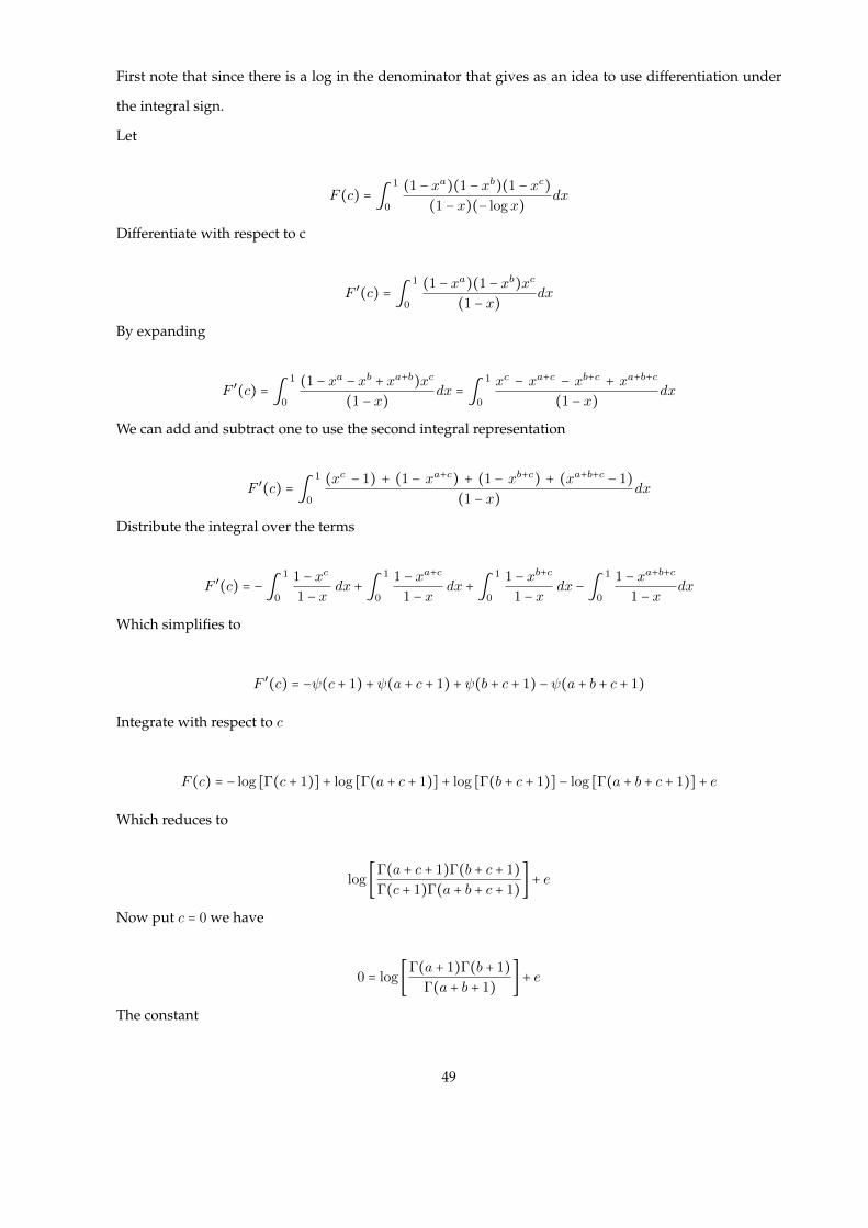
First note that since there is a log in the denominator that gives as an idea to use differentiation under

the integral sign.

Let

F (c) = ∫1

0

(1 − xa)(1 − xb)(1 − xc)(1 − x)(− logx)

dx

Differentiate with respect to c

F ′(c) = ∫1

0

(1 − xa)(1 − xb)xc

(1 − x)dx

By expanding

F ′(c) = ∫1

0

(1 − xa − xb + xa+b)xc

(1 − x)dx = ∫

1

0

xc − xa+c − xb+c + xa+b+c

(1 − x)dx

We can add and subtract one to use the second integral representation

F ′(c) = ∫1

0

(xc − 1) + (1 − xa+c) + (1 − xb+c) + (xa+b+c − 1)(1 − x)

dx

Distribute the integral over the terms

F ′(c) = −∫1

0

1 − xc

1 − xdx + ∫

1

0

1 − xa+c

1 − xdx + ∫

1

0

1 − xb+c

1 − xdx − ∫

1

0

1 − xa+b+c

1 − xdx

Which simplifies to

F ′(c) = −ψ(c + 1) + ψ(a + c + 1) + ψ(b + c + 1) − ψ(a + b + c + 1)

Integrate with respect to c

F (c) = − log [Γ(c + 1)] + log [Γ(a + c + 1)] + log [Γ(b + c + 1)] − log [Γ(a + b + c + 1)] + e

Which reduces to

log [Γ(a + c + 1)Γ(b + c + 1)Γ(c + 1)Γ(a + b + c + 1)

] + e

Now put c = 0 we have

0 = log [Γ(a + 1)Γ(b + 1)Γ(a + b + 1)

] + e

The constant

49

e = − log [Γ(a + 1)Γ(b + 1)Γ(a + b + 1)

]

So we have the following

F (c) = log [Γ(a + c + 1)Γ(b + c + 1)Γ(c + 1)Γ(a + b + c + 1)

] − log [Γ(a + 1)Γ(b + 1)Γ(a + b + 1)

]

Hence we have the result

∫1

0

(1 − xa)(1 − xb)(1 − xc)(1 − x)(− logx)

dx = log{ Γ(b + c + 1)Γ(c + a + 1)Γ(a + b + 1)Γ(a + 1)Γ(b + 1)Γ(c + 1)Γ(a + b + c + 1)

}

5.13 Example


∫∞

0(e−bx − 1

1 + ax) dx

x

Let us first use the substitution t = ax

∫∞

0(e−

bta − 1

1 + t) dt

t

Add and subtract e−t

∫∞

0(e−t − e−t + e−

bta − 1

1 + t) dt

t

Separate into two integrals

∫∞

0(e−t − 1

1 + t) dt

t+ ∫

∞

0

e−bta − e−t

tdt

The first integral is a representation of the Euler constant when a = 1

∫∞

0(e−t − 1

1 + t) dtt= −γ

We also proved

∫∞

0

e−bta − e−t

tdt = − log ( b

a) = log (a

b)

Hence the result

∫∞

0(e−bx − 1

1 + ax) dx

x= log (a

b) − γ

50

5.14 Example


∫∞

0e−ax ( 1

x− coth(x)) dx

By using the exponential representation of the hyperbolic functions

∫∞

0e−ax ( 1

x− 1 + e−2x

1 − e−2x) dx

Now let 2x = t so we have

∫∞

0e−(

at2) (1

t− 1 + e−t

2(1 − e−t)) dt

∫∞

0

e−(at2)

t− e

−( at2 ) + e(− at2 −t)

2(1 − e−t)dt

By adding and subtracting some terms

∫∞

0

e−t + e−( at2 ) − e−t

t− e−(

at2) + e−( at2 ) − e− at2 + e−( at2 )−t

2(1 − e−t)dt

Separate the integrals

∫∞

0

e−t

t− e−(

at2)

1 − e−tdt + ∫

∞

0

e−(at2) − e(− at2 −t)

2(1 − e−t)dt + ∫

∞

0

e−(at2) − e−t

tdt

By using the third integral representation

∫∞

0

e−t

t− e−(

at2)

1 − e−tdt = ψ (a

2)

The second integral reduces to

∫∞

0

e−(at2) − e−( at2 −t)

2(1 − e−t)= ∫

∞

0

e−(at2)

2dt = 1

a

The third integral

∫∞

0

e−(at2) − e−t

tdt = − log (a

2)

By collecting the results

∫∞

0e−ax ( 1

x− coth(x)) dx = ψ (a

2) − log (a

2) + 1

a

51

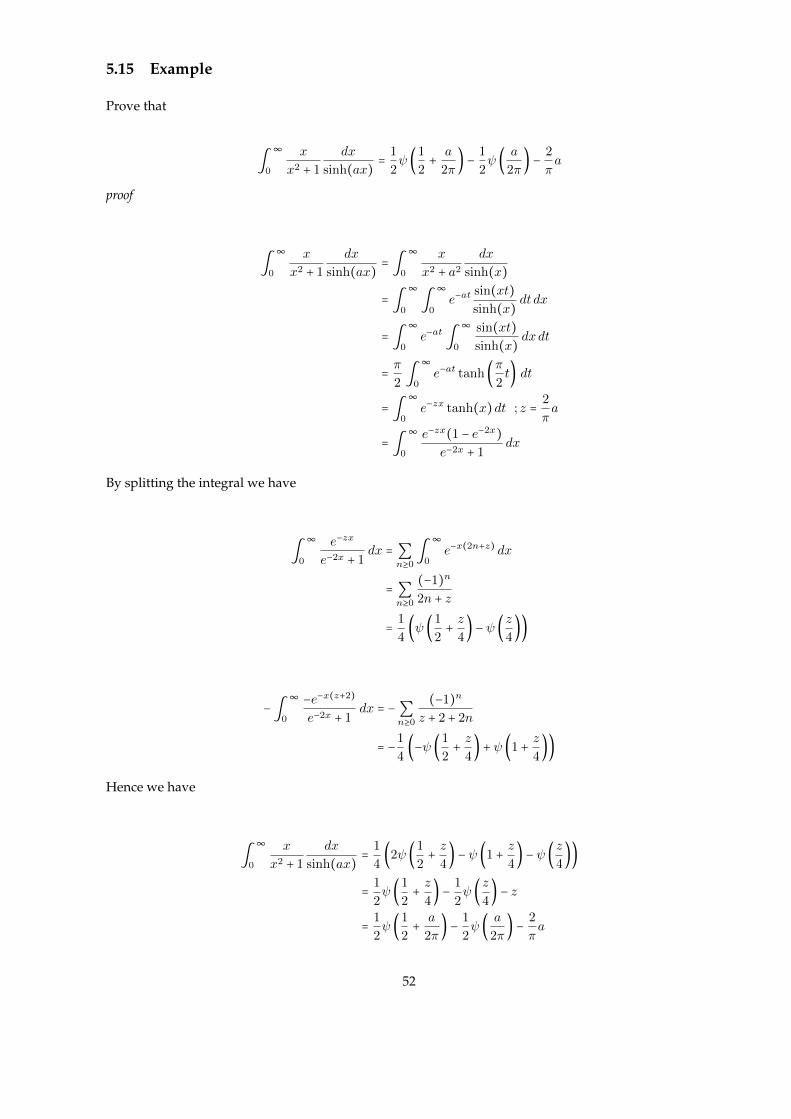
5.15 Example

Prove that

∫∞

0

x

x2 + 1

dx

sinh(ax)= 1

2ψ (1

2+ a

2π) − 1

2ψ ( a

2π) − 2

πa

proof

∫∞

0

x

x2 + 1

dx

sinh(ax)= ∫

∞

0

x

x2 + a2

dx

sinh(x)

= ∫∞

0∫

∞

0e−at

sin(xt)sinh(x)

dt dx

= ∫∞

0e−at ∫

∞

0

sin(xt)sinh(x)

dxdt

= π2∫

∞

0e−at tanh(π

2t) dt

= ∫∞

0e−zx tanh(x)dt ; z = 2

πa

= ∫∞

0

e−zx(1 − e−2x)e−2x + 1

dx

By splitting the integral we have

∫∞

0

e−zx

e−2x + 1dx = ∑

n≥0∫

∞

0e−x(2n+z) dx

= ∑n≥0

(−1)n

2n + z

= 1

4(ψ (1

2+ z

4) − ψ (z

4))

−∫∞

0

−e−x(z+2)

e−2x + 1dx = −∑

n≥0

(−1)n

z + 2 + 2n

= −1

4(−ψ (1

2+ z

4) + ψ (1 + z

4))

Hence we have

∫∞

0

x

x2 + 1

dx

sinh(ax)= 1

4(2ψ (1

2+ z

4) − ψ (1 + z

4) − ψ (z

4))

= 1

2ψ (1

2+ z

4) − 1

2ψ (z

4) − z

= 1

2ψ (1

2+ a

2π) − 1

2ψ ( a

2π) − 2

πa

52

Let a = π/2

∫∞

0

x

x2 + 1

dx

sinh(π2x)

= 1

2ψ (1

2+ 1

4) − 1

2ψ (1

4) − 1

= π2

cot(π/4) − 1

= π2− 1

53

6 Zeta function

Zeta function is one of the most important mathematical functions. The study of zeta function isn’t

exclusive to analysis. It also extends to number theory and the most celebrating theorem of Riemann.

6.1 Definition

ζ(s) =∞∑n=1

1

ns

6.2 Bernoulli numbers

We define the Bernoulli numbers Bk as

x

ex − 1=

∞∑k=0

Bkk!xk

Now let us derive some values for the Bernoulli numbers , rewrite the power series as

x = (ex − 1)∞∑k=0

Bkk!xk

By expansion

x = (x + 1

2!x2 + 1

3!x3 + 1

4!x4 +⋯) ⋅ (B0 +B1 x +

B2

2!x2 + B3

3!x3 +⋯)

By multiplying we get

x = B0x + (B1 +B0

2!)x2 + (B0

3!+ B2

2!+ B1

2!)x3 + (B0

4!+ B1

3!+ B2

2! 2!+ B3

3!)x4 +⋯

By comparing the terms we get the following values

B0 = 1 , B1 = −1

2+ B2 =

1

6, B3 = 0 , B4 = −

1

30,⋯

Actually we also deduce that

B2k+1 = 0 , ∀ k ∈ Z+

54

6.3 Relation between zeta and Bernoulli numbers

According to Euler we have the following relation

ζ(2k) = (−1)k−1B2k22k−1

(2k)!π2k

proof

We start by the product formula of the sine function

sin(z)z

=∞∏n=1

(1 − z2

n2 π2)

Take the logarithm to both sides

log(sin(z)) − log(z) =∞∑n=1

log(1 − z2

n2 π2)

By differentiation with respect to z

cot(z) − 1

z= −2

∞∑n=1

zn2 π2

1 − z2

n2 π2

By simple algebraical manipulation we have

z cot(z) = 1 − 2∞∑n=1

z2

n2 π2

⎛⎝

1

1 − z2

π2 n2

⎞⎠

Now using the power series expansion

1

1 − z2

π2 n2

=∞∑k=0

1

n2k π2kz2k , ∣z∣ < π n

z2

n2 π2

⎛⎝

1

1 − z2

π2 n2

⎞⎠=

∞∑k=0

1

n2k+2 π2k+2z2k+2 =

∞∑k=1

1

n2k π2kz2k

So the sums becomes

z cot(z) = 1 − 2∞∑n=1

∞∑k=1

1

n2k

z2k

π2k

Now if we invert the order of summation we have

z cot(z) = 1 − 2∞∑k=1

∞∑n=1

1

n2k

z2k

π2k= 1 − 2

∞∑k=1

ζ(2k)π2k

z2k

Euler didn’t stop here, he used power series for z cot(z) using the Bernoulli numbers.

Start by the equation

55

x

ex − 1=

∞∑k=0

Bkk!xk

By putting x = 2iz we have

2iz

e2iz − 1=

∞∑k=0

Bkk!

(2iz)k

Which can be reduced directly to the following by noticing that B2k+1 = 0

z cot(z) = 1 −∞∑k=1

(−1)k−1B2k22k

(2k)!z2k

The result is immediate by comparing the two different representations.

6.4 Exercise

Find the values of

ζ(4) , ζ(6) , B5 , B6

6.5 Integral representation

ζ(s) = 1

Γ(s) ∫∞

0

ts−1

et − 1dt

proof

Start by the integral representation

∫∞

0

e−tts−1

1 − e−tdt

Using the power expansion

1

1 − e−t=

∞∑n=0

e−nt

Hence we have

∫∞

0e−tts−1 (

∞∑n=0

e−nt) dt

By swapping the series and integral

∞∑n=0∫

∞

0ts−1e−(n+1)t dt = Γ(s)

∞∑n=0

1

(n + 1)s= Γ(s)ζ(s)

56

6.6 Hurwitz zeta and polygamma functions

Hurwitz zeta is a generalization of the zeta function by adding a parameter .

6.6.1 Definition

ζ(a, z) =∞∑n=0

1

(n + z)a; ζ(a,1) = ζ(a)

Let us define the polygamma function as the function produced by differentiating the Digamma function

and it is often denoted by

ψn(z) ∀ n ≥ 0

We define the digamma function by setting n = 0 so it’s denoted by ψ0(z) .

Other values can be found by the following recurrence relation

ψ′n(z) = ψn+1(z)

So we have

ψ1(z) = ψ′0(z)

6.6.2 Relation between zeta and polygamma

∀ n ≥ 1

ψn(z) = (−1)n+1n! ζ(n + 1, z)

ψ2n−1(1) = (−1)n−1B2n22n−2

nπ2n

proof

We have already proved the following relation

ψ0(z) = −γ −1

z+

∞∑n=1

z

n(n + z)

This can be written as the following

ψ0(z) = −γ +∞∑k=0

1

k + 1− 1

k + z

By differentiating with respect to z

57

ψ1(z) =∞∑k=0

1

(k + z)2

ψ2(z) = −2∞∑k=0

1

(k + z)3

ψ3(z) = 2 ⋅ 3∞∑k=0

1

(k + z)4

ψ4(z) = −2 ⋅ 3 ⋅ 4∞∑k=0

1

(k + z)5

Continue like that to obtain

ψn(z) = (−1)n+1n!∞∑k=0

1

(k + z)n+1

We realize the RHS is just the Hurwitz zeta function

ψn(z) = (−1)n+1n! ζ(n + 1, z)

By setting z = 1 we have an equation in terms of the ordinary zeta function

ψn(1) = (−1)n+1n! ζ(n + 1)

Now since we already proved in the preceding section that

ζ(2k) = (−1)k−1B2k22k−1

(2k)!π2k

we can easily verify the following

ψ2n−1(1) = (2n − 1)! (−1)n−1B2n22n−1

(2n)!π2n = (−1)n−1B2n

22n−2

nπ2n

This can be used to deduce some values for the polygamma function

ψ1(1) =π2

6, ψ3(1) =

π4

15

Other values can be evaluated in terms of the zeta function

ψ2(1) = −2ζ(3) , ψ4(1) = −24ζ(5)

58

6.7 Example

Prove that

∫π2

0x sin(x) cos(x) log(sinx) log(cosx)dx = π

16− π3

192

proof

Start by the transformation x→ π2− x

∫π2


4∫

π2

0sin(x) cos(x) log(sinx) log(cosx)dx

We need to find

∫π2

0sin(x) cos(x) log(sinx) log(cosx)dx

Let us start by the following

F (a, b) = 2∫π2

0sin2a−1(x) cos2b−1(x)dx = Γ(a)Γ(b)

Γ(a + b)

Now let us differentiate with respect to a

∂

∂a(F (a, b)) = 4∫

π2

0sin2a−1(x) cos2b−1(x) log(sinx)dx = Γ(a)Γ(b) (ψ0(a) − ψ0(a + b))

Γ(a + b)

Differentiate again but this time with respect to b

∂

∂b(Fa(a, b)) = 8∫

π2

0sin2a−1(x) cos2b−1(x) log(sinx) log(cosx)dx

=Γ(a)Γ(b) (ψ2

0(a + b) + ψ0(a)ψ0(b) − ψ0(a)ψ0(a + b) − ψ0(b)ψ0(a + b) + ψ1(a + b))Γ(a + b)

Putting a = b = 1 we have the following

∫π2

0sin(x) cos(x) log(sinx) log(cosx)dx = ψ

20(2) + ψ2

0(1) − ψ0(1)ψ0(2) − ψ0(1)ψ(2) − ψ1(2)8

By simple algebra we arrive to

∫π2

0sin(x) cos(x) log(sinx) log(cosx)dx = (ψ0(2) − ψ0(1))2 − ψ1(2)

8

We already know that ψ0(1) = −γ and ψ0(2) = 1 − γ

Now to evaluate ψ1(2) , we have to use the zeta function we have already established the following

relation

59

ψ1(z) =∞∑k=0

1

(n + z)2

Now putting z = 2 we have the following

ψ1(2) =∞∑k=0

1

(k + 2)2

Let us write the first few terms in the expansion

∞∑k=0

1

(k + 2)2= 1

22+ 1

32+ 1

42+⋯

we see this is similar to ζ(2) but we are missing the first term

ψ1(2) = ζ(2) − 1 = π2

6− 1

Collecting all these results together we have

∫π2

0sin(x) cos(x) log(sinx) log(cosx)dx = 1

4− π

2

48

Finally we get our result

∫π2


16− π3

192

60

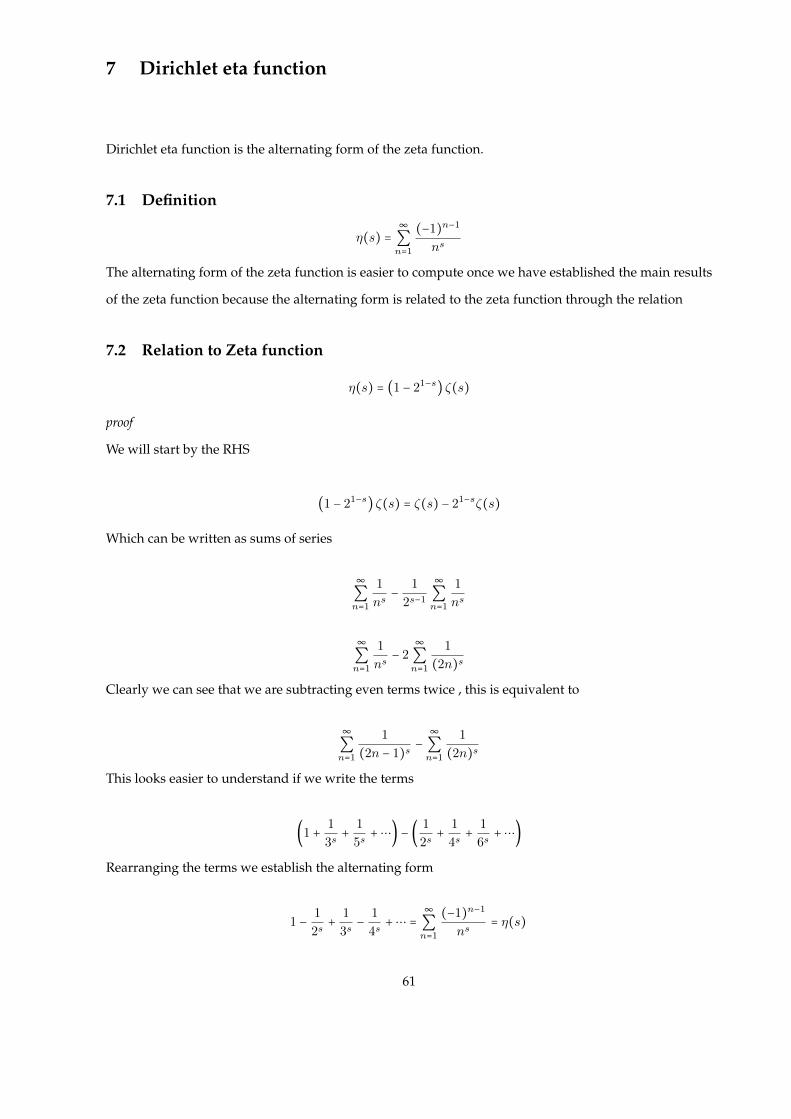
7 Dirichlet eta function

Dirichlet eta function is the alternating form of the zeta function.

7.1 Definition

η(s) =∞∑n=1

(−1)n−1

ns

The alternating form of the zeta function is easier to compute once we have established the main results

of the zeta function because the alternating form is related to the zeta function through the relation

7.2 Relation to Zeta function

η(s) = (1 − 21−s) ζ(s)

proof

We will start by the RHS

(1 − 21−s) ζ(s) = ζ(s) − 21−sζ(s)

Which can be written as sums of series

∞∑n=1

1

ns− 1

2s−1

∞∑n=1

1

ns

∞∑n=1

1

ns− 2

∞∑n=1

1

(2n)s

Clearly we can see that we are subtracting even terms twice , this is equivalent to

∞∑n=1

1

(2n − 1)s−

∞∑n=1

1

(2n)s

This looks easier to understand if we write the terms

(1 + 1

3s+ 1

5s+⋯) − ( 1

2s+ 1

4s+ 1

6s+⋯)

Rearranging the terms we establish the alternating form

1 − 1

2s+ 1

3s− 1

4s+⋯ =

∞∑n=1

(−1)n−1

ns= η(s)

61


η(s)Γ(s) = ∫∞

0

ts−1

et + 1dt

proof

Start by the RHS

∫∞

0

ts−1

et + 1dt = ∫

∞

0

e−tts−1

1 + e−tdt

Now using the power expansion we arrive to

∫∞

0e−tts−1dt(

∞∑n=0

(−1)ne−nt)

∞∑n=0

(−1)n ∫∞

0e−(n+1)tts−1dt

Using Laplace transform we can solve the inner integral

∫∞

0e−(n+1)tts−1dt = Γ(s)

(n + 1)s


Γ(s)∞∑n=0

(−1)n

(n + 1)s= Γ(s)

∞∑n=1

(−1)n−1

ns= Γ(s)η(s)

An easy result of the above integral

∫∞

0

t

et + 1dt = Γ(2)η(2) = π

2

12

62

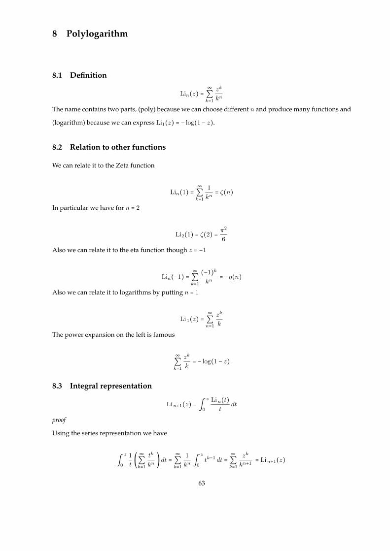
8 Polylogarithm

8.1 Definition

Lin(z) =∞∑k=1

zk

kn

The name contains two parts, (poly) because we can choose different n and produce many functions and

(logarithm) because we can express Li1(z) = − log(1 − z).

8.2 Relation to other functions

We can relate it to the Zeta function

Lin(1) =∞∑k=1

1

kn= ζ(n)

In particular we have for n = 2

Li2(1) = ζ(2) =π2

6

Also we can relate it to the eta function though z = −1

Lin(−1) =∞∑k=1

(−1)k

kn= −η(n)

Also we can relate it to logarithms by putting n = 1

Li1(z) =∞∑n=1

zk

k

The power expansion on the left is famous

∞∑k=1

zk

k= − log(1 − z)


Lin+1(z) = ∫z

0

Lin(t)t

dt

proof

Using the series representation we have

∫z

0

1

t(∞∑k=1

tk

kn)dt =

∞∑k=1

1

kn∫

z

0tk−1 dt =

∞∑k=1

zk

kn+1= Lin+1(z)

63

8.4 Square formula

Lin(−z) + Lin(z) = 21−n Lin(z2)

proof

As usual we write the series representation of the LHS

∞∑k=1

zk

kn+

∞∑k=1

(−z)k

kn

Listing the first few terms

z + z2

2n+ z

3

3n+⋯ + (−z + z

2

2n− z

3

3n+⋯)

The odd terms will cancel

2z2

2n+ 2

z4

4n+ 2

z6

6n+⋯

Take 21−n as a common factor

21−n (z2 + (z2)2

2n+ (z2)3

3n+⋯) = 21−n

∞∑k=1

(z2)k

kn= 21−n Lin(z2)

8.5 Exercise

Prove that

Li2(z) = −∫z

0

log(1 − t)t

dt

64

8.6 Dilogarithms

Of all polylogarithms Li2(z) is the most interesting one, in this section we will see why!

8.6.1 Definition

Li2(z) =∞∑k=1

zk

k2= −∫

z

0

log(1 − t)t

dt

The curious reader should try to prove the integral representation using the recursive definition we

introduced in the previous section .

8.6.2 First functional equation

Li2 (−1

z) + Li2(−z) = −

1

2log2(z) − π

2

6

proof

We will start by the following

Li2 (−1

z) = −∫

−1z

0

log(1 − t)t

dt

Differentiate with respect to z

d

dzLi2 (−1

z) = 1

z2

⎛⎝−

log (1 + 1z)

−1z

⎞⎠=

log (1 + 1z)

z= log(1 + z) − log(z)

z

Now integrate with respect to z

Li2 (−1

z) = ∫

−z

0

log(1 − t)t

dt − 1

2log2(z) +C = −Li2(−z) −

1

2log2(z) +C

To find the constant C let z = 1

C = 2Li2 (−1)

Now we must be aware that

C = 2Li2(−1) = −2η(2) = −π2

6

Which proves the result by simple rearrangement

Li2 (−1

z) + Li2(−z) = −

1

2log2(z) − π

2

6

65

8.6.3 Second functional equation

Li2(z) + Li2(1 − z) =π2

6− log(z) log(1 − z) , 0 < z < 1

proof

Start by the following

Li2 (z) = −∫z

0

log(1 − t)t

dt

Now integrate by parts to obtain

Li2 (z) = −∫z

0

log(t)1 − t

dt − log(z) log(1 − z)

By the change of variable t = 1 − x we get

∫z

0

log(t)1 − t

dt = −∫1−z

1

log(1 − x)x

dx

For 0 < z < 1

∫1

1−z

log(1 − x)x

dx = ∫1

0

log(1 − x)x

dx − ∫1−z

0

log(1 − x)x

dx

Now it is easy to see that

∫1

1−z

log(1 − x)x

dx = −Li2(1) + Li2(1 − z)

Which implies that

Li2 (z) = Li2(1) − Li2(1 − z) − log(z) log(1 − z)

Li2 (z) + Li2(1 − z) = Li2(1) − log(z) log(1 − z)

Now since Li2(1) = ζ(2) = π2

6

Li2 (z) + Li2(1 − z) = π2

6− log(z) log(1 − z)

We can easily deduce that for z = 12

2Li2 (1

2) = π

2

6− log2 (1

2)

Li2 (1

2) = π

2

12− 1

2log2 (1

2)

66

8.6.4 Third functional equation

Li2(z) + Li2 ( z

z − 1) = −1

2log2(1 − z) z < 1

proof


Li2 ( z

z − 1) = −∫

zz−1

0

log(1 − t)t

dt

Differentiate both sides with respect to z

d

dzLi2 ( z

z − 1) = 1

(z − 1)2

⎛⎝

log (1 − zz−1

)zz−1

⎞⎠

Upon simplification we obtain

d

dzLi2 ( z

z − 1) = − log(1 − z)

z(z − 1)

Using partial fractions decomposition

d

dzLi2 ( z

z − 1) = log(1 − z)

1 − z+ log(1 − z)

z

Integrate both sides with respect to z

Li2 ( z

z − 1) = −1

2log2(1 − z) − Li2(z) +C

Put z = −1 to find the constant

Li2 (1

2) = −1

2log2(2) − Li2(−1) +C

Remember that

Li2 (1

2) = π

2

12− 1

2log2 (1

2) , Li2(−1) = −π

2

12

Hence we deduce that C = 0

Li2 ( z

z − 1) = −1

2log2(1 − z) − Li2(z)

Which can be written as

Li2 ( z

z − 1) + Li2(z) = −

1

2log2(1 − z)

67

8.6.5 Example

Prove that

Li2 (√

5 − 1

2) = π

2

10− log2 (

√5 − 1

2)

proof

First we add the two functional equations of this section to obtain

Li2 ( z

z − 1) + 1

2Li2(z2) − Li2(−z) = −

1

2log2(1 − z)

Now let z = 1−√

52

z2 = 1 − 2√

5 + 5

4= 3 −

√5

2Ô⇒ z

z − 1=

√5 − 1

1 +√

5= 3 −

√5

2

Hence we have

3

2Li2 (3 −

√5

2) − Li2 (

√5 − 1

2) = −1

2log2 (

√5 + 1

2)

We already established the following functional equation

Li2(z) + Li2(1 − z) =π2

6− log(z) log(1 − z)

Put z = 3−√

52

Li2 (3 −√

5

2) + Li2 (

√5 − 1

2) = π

2

6− log(3 −

√5

2) log(

√5 − 1

2)

Solving the two representations for Li2 (√

5−12

) we get our result.

8.6.6 Example


I = ∫1

0

log(1 − x) log(x)x

dx

Integrate by parts

I = − log(x)Li2(x)∣10 + ∫1

0

Li2(t)t

dt = Li3(1) =∞∑k=1

1

k3= ζ(3)

68

8.6.7 Example

Evaluate the following integral

∫x

0

log2(1 − t)t

dt , 0 < x < 1

Integrating by parts we get the following

∫x

0

log2(1 − t)t

dt = − log(1 − x)Li2(x) − ∫x

0

Li2(t)1 − t

dt

Now we are left with the following integral

∫x

0

Li2(t)1 − t

dt = ∫1

1−x

Li2(1 − t)t

dt

Using the first functional equation

∫1

1−x

π2

6− Li2(t) − log(1 − t) log(t)

tdt

−π2

6log(1 − x) − ∫

1

1−x

Li2(t)t

dt − ∫1

1−x

log(1 − t) log(t)t

dt

The first integral

∫1

1−x

Li2(t)t

dt = Li3(1) − Li3(1 − x)

The second integral is the same as the first exercise

∫1

1−x


= Li3(1) + log(1 − x)Li2(1 − x) − Li3(1 − x)

Collecting the results together we obtain

∫x

0

Li2(t)1 − t

dt = −π2

6log(1 − x) − Li2(1 − x) log(1 − x) + 2 Li3(1 − x) − 2ζ(3)

Finally we have

∫x

0

log2(1 − t)t

dt = − log(1 − x)Li2(x) +π2

6log(1 − x) + Li2(1 − x) log(1 − x) − 2 Li3(1 − x) + 2ζ(3)

69

8.6.8 Example


I(a) = ∫a

0

x

ex − 1dx

Start by the power expansion of 11−e−x

I(a) = ∫a

0

x

ex − 1dx = ∫

a

0xe−x

∞∑n=0

e−nx

By swapping the integral and the summation

I(a) =∞∑n=0∫

a

0xe−x(n+1) dx

The integral could be solved by parts

I(a) =∞∑n=0

1

(n + 1)2− e

−(n+1)a

(n + 1)2− ae

−(n+1)a

(n + 1)

Distribute the summation to obtain

I(a) = ζ(2) + a log(1 − e−a) − Li2(e−a)

70

9 Ordinary Hypergeometric function

Ordinary or sometimes called the Gauss hypergoemtric function is a generalization of the power expan-

sion definition. Before we start with the definition we will explain some notations.

9.1 Definition

Define the raising factorial as follows

(z)n =

⎧⎪⎪⎪⎪⎨⎪⎪⎪⎪⎩

1 ∶ n = 0

Γ(z+n)Γ(z) ∶ n > 0

Using this definition have

2F1(a, b; c; z) =∞∑n=0

(a)n(b)n(c)n

zn

n!

9.2 Some expansions using the hypergeomtric function

We can represent famous functions using the hypergeomtric function

1. Logarithm

z2F1(1,1; 2;−z) = z∞∑n=0

(1)n(1)n(2)n

(−z)n

n!=

∞∑n=0

(−1)n n!

(n + 1)!zn+1 =

∞∑n=0

(−1)n zn+1

n + 1= log(1 + z)

2. Power function

2F1(a,1; 1; z) =∞∑n=0

(a)n (1)n(1)n

zn

n!=

∞∑n=0

(a)nn!

zn = (1 − z)−a

3. Sine inverse

z 2F1 ( 12, 1

2; 3

2; z2) =

∞∑n=0

( 12)n( 1

2)n

( 32)n

z2n+1

n!=

∞∑n=0

( 12)n

2n + 1

z2n+1

n!=

∞∑n=0

1 ⋅ 3 ⋅ 5⋯(2n − 1)2n n! (2n + 1)

z2n+1


z 2F1 ( 12, 1

2; 3

2; z2) =

∞∑n=0

(2n)!4n (n!)2 (2n + 1)

z2n+1 =∞∑n=0

(2nn)

4n (2n + 1)z2n+1 = arcsin(z)

Now we consider converting the Taylor expansion into the equivalent hypergeomtric representation

Suppose the following

71

2F1(a, b; c; z) =∞∑k=0

tk zk , t0 = 1

Now consider the ratio

tk+1

tk= (k + a)(k + b)

(k + c)(k + 1)z

Using this definition, we can easily find the terms a, b, c.

Let us consider some examples

1. Exponential function

f(z) = ez

The power expansion is

f(z) = ez =∞∑k=0

zk

k!

Hence we have

tk+1

tk= z

k + 1

Comparing to our representation we conclude

ez = 2F1(−,−;−; z)

2. Cosine function

f(z) = cos(z) =∞∑k=0

(−1)kz2k

(2k)!

By the same approach

tk+1

tk= − 1

(2k + 2)(2k + 1)z = 1

(k + 1) (k + 12)−z2

4

Hence we have

cos(z) = 2F1 (−,−;1

2;−z2

4)

72

3. Power function

f(z) = (1 − z)−a =∞∑k=0

(a)kk!

zk

By the same approach

tk+1

tk= (k + a)

(k + 1)z = (k + a)(k + 1)

(k + 1)(k + 1)z

Hence we have

(1 − z)−a = 2F1(a,1; 1; z)

9.3 Exercise

Find the hypergeoemtric representations of the following functions

arcsin(z), sin(z)


β(c − b, b) 2F1(a, b; c; z) = ∫1

0

tb−1(1 − t)c−b−1

(1 − tz)adt

proof

Start by the RHS

∫1

0tb−1(1 − t)c−b−1 (1 − tz)−a dt

Using the expansion of (1 − tz)−a we have

∫1

0tb−1(1 − t)c−b−1

∞∑k=0

(a)kk!

(tz)k

Interchanging the integral with the series

∞∑k=0

(a)kk!

zk ∫1

0tk+b−1(1 − t)c−b−1 dt

Recalling the beta function we have

∞∑n=0

(a)kΓ(k + b)Γ(c − b)Γ(k + c)

zk

k!

73

Using the identity that

β(c − b, b) = Γ(b)Γ(c − b)Γ(c)

and

Γ(z + k)Γ(z)

= (z)k

We deduce that

β(c − b, b)∞∑k=0

(a)kΓ(k + b)Γ(c)Γ(b)Γ(k + c)

zk

k!= β(c − b, b)

∞∑k=0

(a)k(b)k(c)k

zk

k!

9.5 Transformations

1. Pfaff transformations

2F1 (a, b; c; z) = (1 − z)−a2F1 (a, c − b; c; z

z − 1)

and

2F1 (a, b; c; z) = (1 − z)−b2F1 (c − a, b; c; z

z − 1)

proof


2F1 (a, b; c; z) = 1

β(b, c − b) ∫1

0

tb−1(1 − t)c−b−1

(1 − tz)adt

By the the transformation t→ 1 − t

∫1

0

(1 − t)b−1tc−b−1

(1 − (1 − t)z)adt = ∫

1

0

(1 − t)b−1tc−b−1

(1 − z + tz)adt


(1 − z)−a

β(b, c − b) ∫1

0tc−b−1(1 − t)b−1 (1 − t z

z − 1)−adt

Note this is the integral representation of

74

(1 − z)−a2F1 (a, c − b; c; z

z − 1)

Also using that

2F1 (a, b; c; z) = 2F1 (b, a; c; z)

We deduce that

2F1 (a, b; c; z) = (1 − z)−b2F1 (c − a, b; c; z

z − 1)

2. Euler transformation

2F1 (a, b; c; z) = (1 − z)c−a−b2F1 (c − a, c − b; c; z)

proof

In the Pfaff transformations let z → zz−1

2F1 (a, b; c; z

z − 1) = (1 − z)−a2F1 (a, c − b; c; z)

and

2F1 (a, b; c; z

z − 1) = (1 − z)−b2F1 (c − a, b; c; z)

By equating the two transformations

(1 − z)−a2F1 (a, c − b; c; z) = (1 − z)−b2F1 (c − a, b; c; z)

Now use the transformation b→ c − b

(1 − z)−a2F1 (a, b; c; z) = (1 − z)c−b2F1 (c − a, c − b; c; z)

Which can be reduced to

2F1 (a, b; c; z) = (1 − z)c−a−b2F1 (c − a, c − b; c; z)

75

3. Quadratic transformation

2F1 (a, b; 2b; z) = (1 − z)−a2 2F1 (a

2, b − a

2; b + 1

2;

z2

4z − 4)

4. Kummer

2F1 (a, b; c; z) = 2F1 (a, b; 1 + a + b − c; 1 − z)

9.6 Special values

1. At z = 1

2F1(a, b; c; 1) = Γ(c)Γ(c − a − b)Γ(c − a)Γ(c − a)

Start by the integral representation at z = 1

2F1(a, b; c; 1) = 1

β(c − b, b) ∫1

0tb−1(1 − t)c−b−a−1 dt

Now we can use the first integral representation of the beta function

2F1(a, b; c; 1) = 1

β(c − b, b)⋅ Γ(b)Γ(c − b − a)

Γ(c − a)

Which could be simplified to

2F1(a, b; c; 1) = Γ(c)Γ(b)Γ(c − b)

⋅ Γ(b)Γ(c − b − a)Γ(c − a)

= Γ(c)Γ(c − a − b)Γ(c − a)Γ(c − a)

2. At z = −1

2F1(a, b; 1 + a − b;−1) =Γ(1 + a − b)Γ (1 + a

2)

Γ(1 + a)Γ(1 + a2− b)

76

10 Error Function

The error function is an interesting function that has many applications in probability, statistics and

physics.

10.1 Definition

erf(x) = 2√π∫

x

0e−t

2

dt

10.2 Complementary error function

erfc(x) = 1 − erf(x)

10.3 Imaginary error function

erfi(x) = −ierf(ix)

10.4 Properties

1. The error function is odd

erf(−x) = 2√π∫

−x

0e−t

2

dt = − 2√π∫

x

0e−t

2

dt = −erf(x)

2. Real part and imaginary parts

R erf(z) = erf(z) + erf(z̄)2

I erf(z) = erf(z) − erf(z̄)2i

Using complex variables it can be done using erf(z̄) = erf(z)

10.5 Relation to other functions

1. Hypergeomtric function

erf(x) = 2x√π

1F1 (1

2,3

2,−x2)

77

proof

By expanding the hypergeometirc function

2x√π

1F1 (1

2,3

2,−x2) = 2x√

π

∞∑k=0

( 12)k

( 32)k

(−x2)k

k!

Which can be simplified to

2x√π

1F1 (1

2,3

2,−x2) = x√

π

∞∑k=0

(−x2)k

( 12+ k)k!

Notice that this is actually the expanded error function

2√π∫

x

0e−t

2

dt = 2√π∫

x

0

∞∑k=0

(−x2)k

k!dt = 2√

π

∞∑k=0

(−x)2k+1

(2k + 1)k!

2. Incomplete Gamma function

erf(x) = 1 −Γ ( 1

2, x2)

√π

proof

By the definition of the incomplete gamma function

Γ(1

2, x2) = ∫

∞

x2t−

12 e−t dt

Let t = y2

Γ(1

2, x2) = 2∫

∞

xe−y

2

dy

We need to get the interval (0, x)

Γ(1

2, x2) = 2∫

∞

0e−y

2

dy − 2∫x

0e−y

2

dy

We have already proved that

2∫∞

0e−y

2

dy =√π

Hence we have using the definition of the error function

78

Γ(1

2, x2) =

√π −

√πerf(x)

By rearrangements we get our result.

10.6 Example

Find the integral

I = ∫x

0et

2

dt

The function has no elementary anti-derivative so we represent it using the error function.

Consider the imaginary error function

erfi(x) = −i 2√π∫

ix

0e−t

2

dt

By differentiating both sides we have

d

dxerfi(x) = 2√

πex

2

Hence we have

ex2

= d

dx

√π

2erfi(x)

By integrating both sides we have

∫x

0et

2

dt =√π

2erfi(x)

10.7 Example

Prove that

∫∞

0erfc(x)dx = 1√

π

proof

Using the complementary error function

∫∞

0(1 − erf(x))dx

79

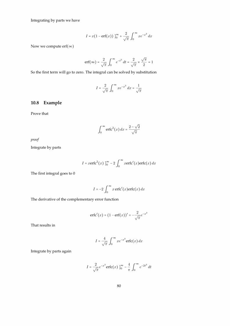
Integrating by parts we have

I = x(1 − erf(x)) ]∞0 + 2√π∫

∞

0xe−x

2

dx

Now we compute erf(∞)

erf(∞) = 2√π∫

∞

0e−t

2

dt = 2√π×

√π

2= 1

So the first term will go to zero. The integral can be solved by substitution

I = 2√π∫

∞

0xe−x

2

dx = 1√π

10.8 Example

Prove that

∫∞

0erfc2(x)dx = 2 −

√2√

π

proof

Integrate by parts

I = xerfc2(x) ]∞0 − 2∫∞

0xerfc′(x)erfc(x)dx

The first integral goes to 0

I = −2∫∞

0x erfc′(x)erfc(x)dx

The derivative of the complementary error function

erfc′(x) = (1 − erf(x))′ = − 2√πe−x

2

That results in

I = 4√π∫

∞

0xe−x

2

erfc(x)dx

Integrate by parts again

I = 2√πe−x

2

erfc(x) ]∞0 − 4

π∫

∞

0e−2t2 dt

80

At infinity the integral goes to 0. At 0 we get

2√πe−x

2

erfc(x)]x=0 =2√π(1 − erf(0)) = 2√

π

The integral can be evaluated to

∫∞

0e−2t2 dt =

√π

2√

2

Collecting the results together we have

I = 2√π−

√π

2√

2× 4

π= 2 −

√2√

π

10.9 Example

Prove that

∫∞

0sin(x2)erfc(x)dx = π − 2 coth−1

√2

4√

2π

proof

Using the substitution x =√t

1

2∫

∞

0sin(t)t−

12 erfc(

√t)dt

Consider the function

I(a) = 1

2∫

∞

0sin(t)t−

12 erfc(a

√t)dt

Differentiating with respect to a we have

I ′(a) = −1√π∫

∞

0sin(t)e−a

2t dt = −1√π⋅ 1

a4 + 1

Now integrating with respect to a

I(a) = −1√π∫

a

0

dx

x4 + 1+C

To evaluate the constant we take a→∞

I(∞) = −1√π∫

∞

0

dx

x4 + 1+C

81

The function has an anti-derivative and the value is

−1√π∫

∞

0

dx

x4 + 1= −

√π

2√

2

Note that

erfc(∞) = 0 Ô⇒ C =√π

2√

2

Finally we get

I(a) = −1√π∫

a

0

dx

x4 + 1+

√π

2√

2

Let a = 1 in the integral

I(1) = ∫∞

0sin(x2)erfc(x)dx =

√π

2√

2− 1√

π∫

1

0

dx

x4 + 1

Also knowing that

1√π∫

1

0

dx

x4 + 1= π + 2 coth−1

√2

4√

2π

Hence we have the result

∫∞

0sin(x2)erfc(x)dx = π − 2 coth−1

√2

4√

2π

10.10 Exercise

Can you find closed forms for

∫∞

0erfc3(x)dx =?

∫∞

0erfc4(x)dx =?

What about

∫∞

0erfcn(x)dx =?

82

11 Exponential integral function

11.1 Definition

E(x) = ∫∞

x

e−t

tdt = ∫

∞

1

e−xt

tdt

11.2 Example

Prove that

limx→0

[log(x) +E(x)] = −γ

proof

Integration by parts for E(x)

E(x) = e−t log(t) ]∞x + ∫∞

xlog(t)e−t dt

The limit at infinity goes to zero

E(x) = −e−x log(x) + ∫∞

xlog(t)e−t dt

Hence by taking the limit

limx→0

[log(x) +E(x)] = limx→0

(log(x) − e−x log(x)) + ∫∞

0log(t)e−t dt

The first limit goes to 0

limx→0

[log(x) +E(x)] = ∫∞

0log(t)e−t dt = ψ(1) = −γ

11.3 Example

Prove that for p > 0

∫∞

0xp−1E(ax)dx = Γ(p)

pap

proof

Integrating by parts we have

83

∫∞

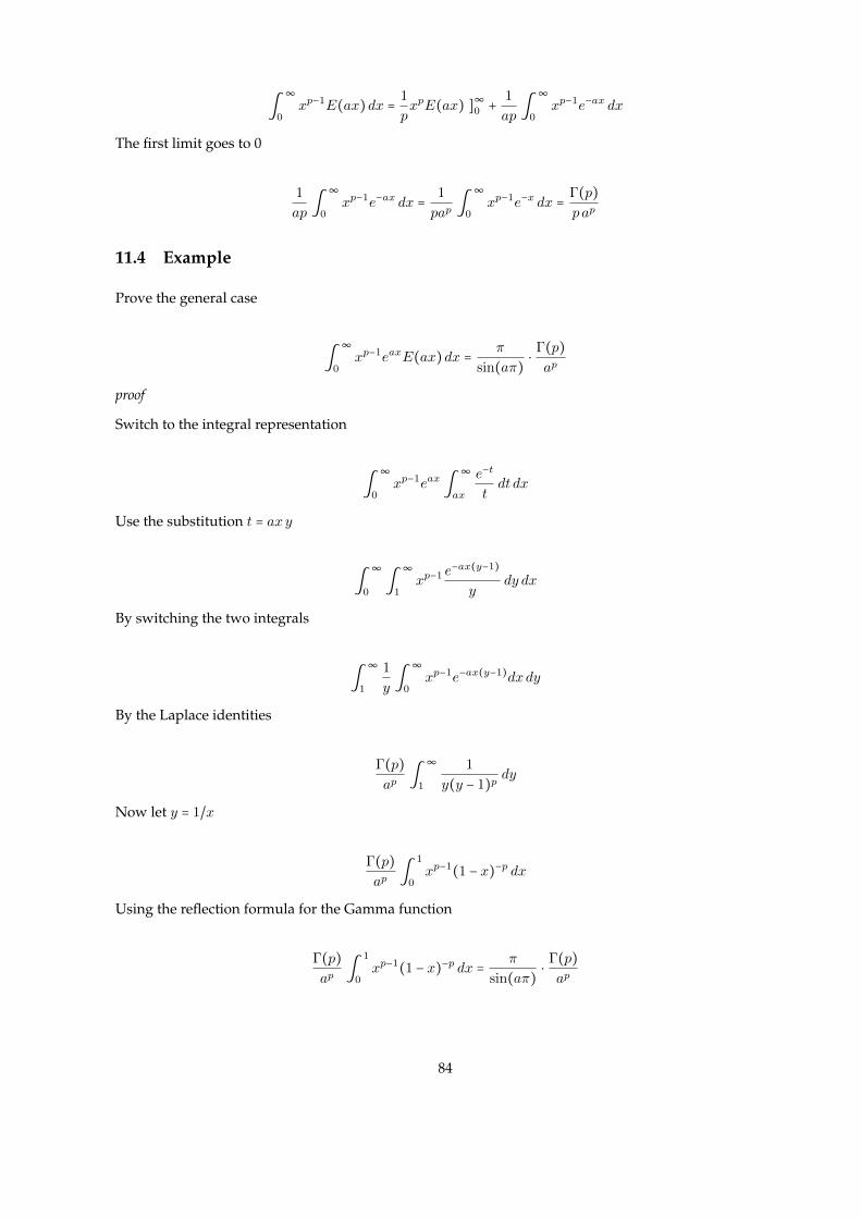
0xp−1E(ax)dx = 1

pxpE(ax) ]∞0 + 1

ap∫

∞

0xp−1e−ax dx

The first limit goes to 0

1

ap∫

∞

0xp−1e−ax dx = 1

pap∫

∞

0xp−1e−x dx = Γ(p)

pap

11.4 Example

Prove the general case

∫∞

0xp−1eaxE(ax)dx = π

sin(aπ)⋅ Γ(p)ap

proof

Switch to the integral representation

∫∞

0xp−1eax ∫

∞

ax

e−t

tdt dx

Use the substitution t = axy

∫∞

0∫

∞

1xp−1 e

−ax(y−1)

ydy dx

By switching the two integrals

∫∞

1

1

y∫

∞

0xp−1e−ax(y−1)dxdy

By the Laplace identities

Γ(p)ap∫

∞

1

1

y(y − 1)pdy

Now let y = 1/x

Γ(p)ap∫

1

0xp−1(1 − x)−p dx

Using the reflection formula for the Gamma function

Γ(p)ap∫

1

0xp−1(1 − x)−p dx = π

sin(aπ)⋅ Γ(p)ap

84

11.5 Example

Prove that

∫∞

0ezE2(z)dz = π

2

6

proof

Using the integral representation

E2(z) = ∫∞

1∫

∞

1

e−xze−yz

xydxdy

∫∞

0ezE2(z)dz = ∫

∞

0∫

∞

1∫

∞

1

e−z(x+y−1)

xydxdy dz

Swap the integrals

∫∞

1

1

y∫

∞

1

1

x∫

∞

0e−z(x+y−1) dz dxdy

∫∞

1

1

y∫

∞

1

1

x(x + y − 1)dxdy

The inner integral is an elementary integral

∫∞

1

1

x(x + y − 1)dx = − log(y)

1 − y

The integral becomes

∫∞

1

log(y)y(y − 1)

dy

Now use the substitution y = 1/x

−∫1

0

log(x)(1 − x)

dx = −∫1

0

log(1 − x)x

dx = Li2(1) =π2

6

11.6 Example

Prove that

∫∞

0zp−1E2(z)dz = 2Γ(p)

p2 2F1(p, p;p + 1;−1)

proof

85

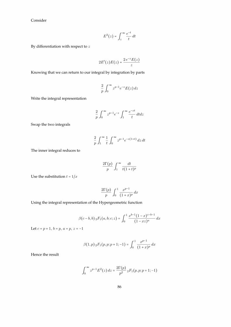
Consider

E2(z) = ∫∞

z

e−t

tdt

By differentiation with respect to z

2E′(z)E(z) = 2 e−zE(z)z

Knowing that we can return to our integral by integration by parts

2

p∫

∞

0zp−1e−zE(z)dz

Write the integral representation

2

p∫

∞

0zp−1e−z ∫

∞

1

e−zt

tdtdz

Swap the two integrals

2

p∫

∞

1

1

t∫

∞

0zp−1e−z(1+t) dz dt

The inner integral reduces to

2Γ(p)p∫

∞

1

dt

t(1 + t)p

Use the substitution t = 1/x

2Γ(p)p∫

1

0

xp−1

(1 + x)pdx

Using the integral representation of the Hypergeometric function

β(c − b, b) 2F1(a, b; c; z) = ∫1

0

xb−1(1 − x)c−b−1

(1 − xz)adx

Let c = p + 1, b = p, a = p, z = −1

β(1, p) 2F1(p, p;p + 1;−1) = ∫1

0

xp−1

(1 + x)pdx

Hence the result

∫∞

0zp−1E2(z)dz = 2Γ(p)

p2 2F1(p, p;p + 1;−1)

86

Where

β(1, p) = Γ(p)Γ(p + 1)

= 1

p

11.7 Exercise

Find the integral fo n ∈ N

∫∞

0xnE2(x)dx

87

12 Complete Elliptic Integral

12.1 Complete elliptic of first kind

K(k) = ∫π2

0

dθ√1 − k2 sin2 θ

= ∫1

0

dx√1 − x2

√1 − k2x2

12.2 Complete elliptic of second kind

E(k) = ∫π2

0

√1 − k2 sin2 θ dθ = ∫

1

0

√1 − k2x2

√1 − x2

dx

12.3 Hypergeometric representation

K(k) = π2

2F1 (1

2,1

2,1, k2)

and

E(k) = π2

2F1 (1

2,−1

2,1, k2)

proof

Using the integral representation of the hypergeometric function

β(c − b, b) 2F1(a, b, c, z) = ∫1

0

tb−1(1 − t)c−b−1

(1 − tz)adt

Now use the substitution t = x2 and z = k2

β(c − b, b) 2F1(a, b, c, k2) = 2∫1

0

x2b−1(1 − x2)c−b−1

(1 − k2x2)adx

Put a = 12

; b = 12

and c = 1

∫1

0

dx√1 − x2

√1 − k2x2

= 1

2β(1/2,1/2) 2F1 (1

2,1

2,1, k2)

By the beta function we have

1

2β(1/2,1/2) = 1

2Γ2 (1

2) = π

2

Hence the result

K(k) = π2

2F1 (1

2,1

2,1, k2)

88

By the same approach we have

E(k) = π2

2F1 (1

2,−1

2,1, k2)

12.4 Example

Prove that

∫1

0K(k)dk = 2G

G is the Catalan’s constant.

proof


I = ∫1

0∫

1

0

1√1 − x2

√1 − k2x2

dxdk

Switching the two integrals

I = ∫1

0

1√1 − x2

∫1

0

1√1 − k2x2

dk dx

I = ∫1

0

arcsinx

x√

1 − x2dx

Now let arcsinx = t hence we have x = sin t

I = ∫π2

0

t

sin tdt

The previous integral is a representation of the constant

G = I2Ô⇒ I = 2G

12.5 Identities

1. For k ≥ 1

K(√k) = 1√

1 − kK

⎛⎝

√k

k − 1

⎞⎠

and

89

E(√k) =

√1 − kE

⎛⎝

√k

k − 1

⎞⎠

proof

Starting by the integral representation

K(k) = ∫1

0

dx√1 − x2

√1 − k2x2

Use the substitution x =√

1 − y2

∫1

0

y dy√1 − y2

√1 − (1 − y2)

√1 − k2(1 − y2)

By cancelling the terms we have

∫1

0

dy√1 − y2

√1 − k2 + k2y2

Take√

1 − k2 as a common factor

∫1

0

dy√

1 − k2√

1 − y2√

1 − k2

k2−1y2

Comparing this to the integral representation we get

K(k) = 1√1 − k2

K⎛⎝

√k2

k2 − 1

⎞⎠

We can finish by k →√k

K(√k) = 1√

1 − kK

⎛⎝

√k

k − 1

⎞⎠

Similarly for the second representation

E(√k) = ∫

1

0

√1 − kx2

√1 − x2

dx

By using that x =√

1 − y2

E(√k) =

√1 − k∫

1

0

√1 − k

k−1y

√1 − y2

dy =√

1 − kE⎛⎝

√k

k − 1

⎞⎠

90

2.

K(k) = 1

k + 1K ( 2

√k

1 + k)

proof

Start by the Quadratic transformation

2F1 (a, b,2b, 4z

(1 + z)2) = (1 + z)2a

2F1 (a, a − b + 1

2, b + 1

2, z2) .

Hence we can deduce by putting a = b = 1/2

K ( 2√k

1 + k) = (1 + k)K(k)

Or we have

K(k) = 1

k + 1K ( 2

√k

1 + k)

3.

K ( 2√k

1 + k) = 1 + k

1 − kK (2

√−k

1 − k)

and

E ( 2√k

1 + k) = 1 − k

1 + kE (2

√−k

1 − k)

proof


K ( 2√k

1 + k) = ∫

1

0

1√

1 − x2√

1 − 4k(1+k)2x

2dx

By some simplifications we have

E ( 2√k

1 + k) = (1 + k)∫

1

0

1√1 − x2

√(1 + k)2 − 4k x2

dx

Use x =√

1 − y2

∫1

0

1 + k√1 − y2

√(1 + k)2 − 4k (1 − y2)

dy = 1 + k1 − k ∫

1

0

1√

1 − y2√

1 + 4k(1−k)2 y

2dy

91

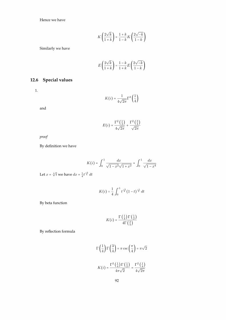
Hence we have

K ( 2√k

1 + k) = 1 + k

1 − kK (2

√−k

1 − k)

Similarly we have

E ( 2√k

1 + k) = 1 − k

1 + kE (2

√−k

1 − k)

12.6 Special values

1.

K(i) = 1

4√

2πΓ2 (1

4)

and

E(i) =Γ2 ( 1

4)

4√

2π+

Γ2 ( 34)

√2π

proof


K(i) = ∫1

0

dx√1 − x2

√1 + x2

= ∫1

0

dx√1 − x4

Let x = 4√t we have dx = 1

4t−34 dt

K(i) = 1

4∫

1

0t−34 (1 − t)

−12 dt

By beta function

K(i) =Γ ( 1

4)Γ ( 1

2)

4Γ ( 34)

By reflection formula

Γ(1

4)Γ(3

4) = π csc(π

4) = π

√2

K(i) =Γ2 ( 1

4)Γ ( 1

2)

4π√

2=

Γ2 ( 14)

4√

2π

92

E(i) =Γ2 ( 1

4)

4√

2π+

Γ2 ( 34)

√2π


E(i) = ∫1

0

√1 + x2

√1 − x2

dx

Separating the two integrals

E(i) = ∫1

0

1 + x2

√1 − x4

dx = ∫1

0

1√1 − x4

dx + ∫1

0

x2

√1 − x4

dx

The first integral is K(i) for the second integral use x = 4√t

1

4∫

1

0t34−1(1 − t)−

12 dt =

Γ ( 34)Γ ( 1

2)

4Γ ( 54)

=Γ2 ( 3

4)

√2π

Hence we have

E(i) =K(i) +Γ2 ( 3

4)

√2π

=Γ2 ( 1

4)

4√

2π+

Γ2 ( 34)

√2π

2.

K ( 1√2) = 1

4√π

Γ2 (1

4)

and

E ( 1√2) =

Γ2 ( 14)

8√π

+Γ2 ( 3

4)

2√π

proof

Start by the identity

K(√k) = 1√

1 − kK

⎛⎝

√k

k − 1

⎞⎠

For the value k = −1

K(i) = 1√2K ( 1√

2)

Using the value for K(i)

93

K ( 1√2) =

√2K(i) = 1

4√π

Γ2 (1

4)

Similarly we have

E ( 1√2) =

Γ2 ( 14)

8√π

+Γ2 ( 3

4)

2√π

3.

K (2√−4 + 3

√2) = 1 +

√2

4√

2πΓ2 (1

4)

and

E (2√−4 + 3

√2) =

√2

1 +√

2

⎡⎢⎢⎢⎣

Γ2 ( 14)

8√π

+Γ2 ( 3

4)

√π

⎤⎥⎥⎥⎦

proof

Start by the identity

K(k) = 1

k + 1K ( 2

√k

1 + k)

Hence we have for k = 1√2

K (2√−4 + 3

√2) = 1 +

√2√

2K ( 1√

2) = 1 +

√2

4√

2πΓ2 (1

4)

For the elliptic integral of second kind using the hypergeomtric representation with a = −12

and

b = 12

2F1 (−1/2,1/2,1, 4z

(1 + z)2) = (1 + z)−1

2F1 (−1/2,−1/2,1, z2)

The later hypergeometric series can be written in terms of elliptic integrals using some general

contiguity relations

2F1 (−1/2,−1/2,1, z2) = 2

π(2E(k) + (k2 − 1)K(k))

So we have

2E(k) + (k2 − 1)K(k) = (k + 1)E ( 2√k

1 + k)

94

For k = 1√2

E (2√−4 + 3

√2) =

√2

1 +√

2

⎡⎢⎢⎢⎣

Γ2 ( 14)

8√π

+Γ2 ( 3

4)

√π

⎤⎥⎥⎥⎦

4.

K (2√−4 − 3

√2) = π

√π

4⋅ 2 −

√2

Γ2 ( 34)

and

E (2√−4 − 3

√2) =

(2 +√

2) (π2 + 4Γ4 ( 34))

4√πΓ2 ( 3

4)

proof

Start by the following identity

K ( 2√k

1 + k) = 1 + k

1 − kK (2

√−k

1 − k)

Let x = 1/√

2

K (2√−4 − 3

√2) = π

√π

4⋅ 2 −

√2

Γ2 ( 34)

E (2√−4 − 3

√2) =

(2 +√

2) (π2 + 4Γ4 ( 34))

4√πΓ2 ( 3

4)

12.7 Differentiation of elliptic integrals

Note We should remove the variable k and denote elliptic integrals E and K once there is no confusion.

It is assumed that the variable is k when we use these symbols.

Interestingly the derivative of elliptic integrals can be written in terms of elliptic integrals

Derivative of complete elliptic integral of second kind

d

dkE = ∫

1

0

∂∂ k

√1 − k2x2

√1 − x2

dx

d

dkE = ∫

1

0

−k x2

√1 − x2

√1 − k2 x2

dx

Adding and subtracting 1 results in

1

k∫

1

0

√1 − k2x2

√1 − x2

dx − 1

k∫

1

0

dx√1 − x2

√1 − k2 x2

95

Upon realizing the relation to elliptic integrals we conclude

d

dkE = E −K

k

For the complete elliptic integral of first kind we need more work


d

dkK = ∫

1

0

1√1 − x2

∂

∂ k[ 1√

1 − k2x2]dx

d

dkK = ∫

1

0

kx2

√1 − x2

√1 − k2x2(1 − k2x2)

dx

Adding and subtracting 1 we have

−1

k∫

1

0

1 − kx2 − 1√1 − x2

√1 − k2x2(1 − k2x2)

dx = 1

k∫

1

0

dx√1 − x2

√1 − k2x2(1 − k2x2)

− Kk

Let us focus on the first integral

∫1

0

1√1 − x2(1 − k2 x2) 3

2

dx

Let x =√t and we have dx = 1

2√tdt

1

2∫

1

0

t−12

√1 − t(1 − k2 t) 3

2

dx

Using the hypergeometric integral representation

1

2∫

1

0

t−12

√1 − t(1 − k2 t) 3

2

= π2

2F1 (3

2,1

2,1, k2)

Using the linear transformation

2F1 (a, b, c, z) = (1 − z)c−a−b 2F1 (c − a, c − b, c, z)

We get by putting k′ =√

1 − k2

π

22F1 (3

2,1

2,1, k2) = 1

1 − k2

π

22F1 (−1

2,1

2,1, k2) = E

k′2

So finally we get

d

dkK = 1

k( Ek′2

−K)

96

13 Euler sums

13.1 Definition

Spr,q =∞∑k=1

(H(p)k )r

kq

Where we define the general harmonic number

H(p)k =

k

∑n=1

1

np; H

(1)k ≡Hk =

k

∑n=1

1

n

Euler sums were greatly studied by Euler, hence the name.

13.2 Generating function∞∑k=1

H(p)k xk =

Lip(x)1 − x

Proof

Start by writing H(p)k as a sum

∞∑k=1

H(p)k xk =

∞∑k=1

k

∑n=1

1

npxk

By interchanging the two series we have

∞∑n=1

∞∑k=n

xk

np=

∞∑n=1

1

np

∞∑k=n

xk

The inner sum is a geometric series

1

1 − x

∞∑n=1

xn

np=

Lip(x)1 − x

We can use this to generate some more functions by integrating.

13.3 Integral representation of Harmonic numbers

Hn = ∫1

0

1 − xn

1 − xdx

proof

We can use the geometric series of xn

∫1

0

1 − xn

1 − xdx =

∞∑k=0∫

1

0xk − xn+k dx

97

∞∑k=0

1

k + 1− 1

n + k + 1=Hn

13.4 Example∞∑n=1

Hn

n2= 2ζ(3)

proof


∫1

0

1

1 − x

∞∑n=1

1 − xn

n2dx = ∫

1

0

ζ(2) − Li2(x)1 − x

dx

Now use the functional equation

ζ(2) − Li2(x) = Li2(1 − x) + log(x) log(1 − x)

Hence we have

∫1

0

Li2(1 − x) + log(x) log(1 − x)1 − x

dx

The first integral

∫1

0

Li2(1 − x)1 − x

= Li3(1) = ζ(3)

The Second integral using integration by parts

∫1

0

log(1 − x) log(x)x

dx = ∫1

0

Li2(x)x

= ζ(3)

Finally we have

∞∑n=1

Hn

n2= ζ(3) + ζ(3) = 2ζ(3)

13.5 Example∞∑k=1

Hk

k2xk = Li3(x) − Li3(1 − x) + log(1 − x)Li2(1 − x) +

1

2log(x) log2(1 − x) + ζ(3)

proof

In the general definition assume p = 1

98

∞∑k=1

Hkxk = − log(1 − x)

1 − x

Divide by x and integrate to get

∞∑k=1

Hk

kxk = Li2(x) +

1

2log2(1 − x)

Now divide by x and integrate again

∞∑k=1

Hk

k2xk = Li3(x) +

1

2∫

x

0

log2(1 − t)t

dt

Now let us look at the integral

∫x

0

log2(1 − t)t

dt

Integrating by parts

∫x

0

log2(1 − t)t

dt = − log(1 − x)Li2(x) − ∫x

0

Li2(t)1 − t

dt

Use a change of variable in the integral

∫x

0

Li2(t)1 − t

dt = ∫1

1−x

Li2(1 − t)t

dt

Now we can use the second functional equation of the dilogarithm

∫1

1−x

π2

6− Li2(t) − log(1 − t) log(t)

tdt


−π2

6log(1 − x) − ∫

1

1−x

Li2(t)t

dt − ∫1

1−x


dt

The first integral

∫1

1−x

Li2(t)t

dt = Li3(1) − Li3(1 − x)

Use integration by parts in the second integral

∫1

1−x


= Li3(1) + log(1 − x)Li2(1 − x) − Li3(1 − x)

Collecting the results together we obtain

99

∫x

0

Li2(t)1 − t

dt = −π2

6log(1 − x) − Li2(1 − x) log(1 − x) + 2 Li3(1 − x) − 2ζ(3)

Hence we solved the integral

∫x

0

log2(1 − t)t

dt = − log(1 − x)Li2(x) +π2

6log(1 − x) + Li2(1 − x) log(1 − x) − 2 Li3(1 − x) + 2ζ(3)

So we have got our Harmonic sum

∞∑k=1

Hk

k2xk = Li3(x) +

1

2(− log(1 − x)Li2(x) +

π2

6log(1 − x) + Li2(1 − x) log(1 − x) − 2 Li3(1 − x) + 2ζ(3))

∞∑k=1

Hk

k2xk = Li3(x) − Li3(1 − x) + log(1 − x)Li2(1 − x) +

1

2log(x) log2(1 − x) + ζ(3)

13.6 General formula∞∑n=1

Hn

nq= (1 + q

2) ζ(q + 1) − 1

2

q−2

∑k=1

ζ(k + 1)ζ(q − k)

This can be proved using complex analysis.

13.7 Example

∫1

0

log2(1 − x) log(x)x

= − π4

180

proof

Using the generating function

∞∑k=1

Hkxk−1 = − log(1 − x)

x(1 − x)

By integrating both sides

∞∑k=1

Hk

kxk = Li2(x) +

1

2log2(1 − x)

Or

log2(1 − x) = 2∞∑k=1

Hk

kxk − 2Li2(x)

plugging this in our integral we have

100

2∫1

0(∞∑k=1

Hk

kxk − Li2(x))

log(x)x

dx

Which simplifies to

2∞∑k=1

Hk

k∫

1

0log(x)xk−1 dx − 2∫

1

0Li2(x)

log(x)x

dx

The second integral

−2∫1

0Li2(x)

log(x)x

dx = 2∫1

0

Li3(x)x

dx = 2ζ(4)

The first integral

2∞∑k=1

Hk

k∫

1

0xk−1 log(x)dx

Using integration by parts twice and the general formula for q = 3

−2∞∑k=1

Hk

k3= −5ζ(4) + ζ2(2)

Finally we get

∫1

0

log2(1 − x) log(x)x

= −5ζ(4) + ζ2(2) + 2ζ(4) = ζ2(2) − 3ζ(4)

13.8 Example

Show that

∫∞

0e−at sin(bt) log t

tdt = −( log(a2 + b2)

2+ γ)arctan( b

a)

Proof

We can start by the following integral

I(s) = ∫∞

0ts−1 e−at sin(bt)dt

By using the the expansion of the sine function

I(s) = ∫∞

0ts−1 e−at

∞∑n=0

(−1)n(bt)2n+1

Γ(2n + 2)

By swapping the summation and integration

101

I(s) =∞∑n=0

(−1)n(b)2n+1

Γ(2n + 2) ∫∞

0ts+2n e−atdt = 1

as

∞∑n=0

(−1)n(b)2n+1Γ(s + 2n + 1)Γ(2n + 2)a2n+1

By differentiating and plugging s = 0 we have

I ′(0) =∞∑n=0

(−1)nψ0(2n + 1)2n + 1

( ba)

2n+1

− log(a)∞∑n=0

(−1)n

2n + 1( ba)

2n+1

Now use that ψ(n + 1) + γ =Hn

I ′(0) =∞∑n=0

(−1)nH2n − γ2n + 1

( ba)

2n+1

− log(a)arctan( ba)

I ′(0) =∞∑n=0

(−1)nH2n

2n + 1( ba)

2n+1

− (γ + log(a))arctan( ba)

Now we look at the harmonic sum

∞∑k=0

(−1)kH2kx2k =

∞∑k=0

(−1)kx2k ∫1

0

1 − t2k

1 − tdt

Use the integral representation

∫1

0

1

1 − t

∞∑k=0

(−1)kx2k (1 − t2k) dt

Swap the series and the integral

∫1

0

1

1 − t

∞∑k=0

(−1)k (x2k − (xt)2k) dt

Evaluate the geometric series

∫1

0

1

1 − t( 1

1 + x2− 1

1 + t2x2) dt = −x2

1 + x2 ∫1

0

(1 − t2)(1 − t)(1 + t2x2)

dt

which simplifies to

−x2

1 + x2 ∫1

0

1 + t(1 + t2x2)

dt = −x2

1 + x2(∫

1

0

1

1 + t2x2+ t

1 + t2x2dt)

Evaluating the integrals

−1

2(1 + x2)(2xarctan(x) + log(1 + x2))

Using this we conclude by integrating

∞∑k=0

(−1)kH2k

2k + 1x2k = −1

2log(1 + x2)arctan(x)

102

Hence the following

∞∑k=0

(−1)kH2k

2k + 1( ba)

2k+1

= −1

2log(a

2 + b2

a2)arctan( b

a)

Substituting that in our integral

∫∞

0e−at sin(bt) log t

tdt = −(1

2log(a

2 + b2

a2) + γ + log(a))arctan( b

a)

= −( log(a2 + b2)2

+ γ)arctan( ba)

13.9 Example

∫1

0

Lip(x) Liq(x)x

dx =p−1

∑n=1

(−1)n−1ζ(p − n + 1)ζ(q + n) − 1

2

p+q−2

∑n=1

(−1)p−1ζ(n + 1)ζ(p + q − n)

+ (−1)p−1 (1 + p + q2

) ζ(p + q + 1)

proof

We can see that

∫1

0

Lip(x) Liq(x)x

dx =∞∑k=1

∞∑n=1

1

kqnp(n + k)

Let us first look at the following

C (α, k) =∞∑n=1

1

nα(n + k); C (1, k) = Hk

k

This can be solved using

C (α, k) =∞∑n=1

1

k nα−1( 1

n− 1

n + k)

= 1

kζ(α) − 1

kC (α − 1, k)

= 1

kζ(α) − 1

k2ζ(α − 1) + 1

k2C (α − 2, k)

⋅

⋅

⋅

= 1

kζ(α) − 1

k2ζ(α − 1) +⋯ + (−1)α ζ(2)

kα−1+ 1

kα−1C (α − (α − 1), k)

=α−1

∑n=1

(−1)n−1 ζ(α − n + 1)kn

+ (−1)α−1Hk

kα

103

Hence we have the general formula

C (α, k) =α−1

∑n=1

(−1)n−1 ζ(α − n + 1)kn

+ (−1)α−1Hk

kα

Dividing by kβ and summing w.r.t to k

∞∑k=1

C (α, k)kβ

=α−1

∑n=1

(−1)n−1ζ(α − n + 1)ζ(β + n) + (−1)α−1∞∑k=1

Hk

kα+β

Now we use the general formula

∞∑n=1

Hn

nq= (1 + q

2) ζ(q + 1) − 1

2

q−2

∑k=1

ζ(k + 1)ζ(q − k)

Hence we have

∞∑n=1

Hn

nα+β= (1 + α + β

2) ζ(α + β + 1) − 1

2

α+β−2

∑k=1

ζ(k + 1)ζ(α + β − k)

And the generalization is the following formula

∞∑k=1

C (α, k)kβ

=α−1

∑n=1

(−1)n−1ζ(α − n + 1)ζ(β + n) − 1

2

α+β−2

∑n=1

(−1)α−1ζ(n + 1)ζ(α + β − n)

+ (−1)α−1 (1 + α + β2

) ζ(α + β + 1)

We conclude by putting that

∞∑k=1

∞∑n=1

1

kqnp(n + k)=

∞∑k=1

C (p, k)kq

13.10 Relation to polygamma

We can relate the generalized harmonic number to the polygamma function

H(p)k = ζ(p) + (−1)p−1ψp−1(k + 1)

(p − 1)!

proof

H(p)k =

k

∑n=1

1

np= ζ(p) −

∞∑

n=k+1

1

np

Now change the index in the sum n = i + k + 1

H(p)k =

k

∑n=1

1

np= ζ(p) −

∞∑i=0

1

(i + k + 1)p

104

We know that

(−1)pψp−1(k + 1)

(p − 1)!=

∞∑i=0

1

(i + k + 1)pp ≥ 1

Hence we have

H(p)k = ζ(p) + (−1)p−1ψp−1(k + 1)

(p − 1)!

We can use that to obtain a nice integral representation.

13.11 Integral representation for r=1∞∑k=1

H(p)k

kq= ζ(p)ζ(q) + (−1)p 1

(p − 1)! ∫1

0

Liq(x) log(x)p−1

1 − xdx

proof

Note that

ψ0(a + 1) = ∫1

0

1 − xa

1 − xdx

By differentiating with respect to a , p times we have

ψp(a + 1) = ∂

∂ap∫

1

0

1 − xa

1 − xdx

ψp(a + 1) = −∫1

0

xa log(x)p

1 − xdx

Let a = k

ψp−1(k + 1) = −∫1

0

xk log(x)p−1

1 − xdx

Use the relation to polygamma

H(p)k = ζ(p) + (−1)p 1

(p − 1)! ∫1

0

xk log(x)p−1

1 − xdx

Now divide by kq and sum with respect to k

∞∑k=1

H(p)k

kq= ζ(p)ζ(q) + (−1)p 1

(p − 1)! ∫1

0

Liq(x) log(x)p−1

1 − xdx

105

13.12 Symmetric formula∞∑k=1

H(p)k

kq+

∞∑k=1

H(q)k

kp= ζ(p)ζ(q) + ζ(p + q)

proof

Take the leftmost series and swap the finite and infinite sums

∞∑i=1

∞∑k=i

1

ip1

kq=

∞∑i=1

∞∑k=1

1

ip1

kq−

∞∑i=1

1

ip

i−1

∑k=1

1

kq

The second sum can be written as

∞∑i=1

1

ip

i−1

∑k=1

1

kq=

∞∑i=1

1

ip(i

∑k=1

1

kq− 1

ip)

By separating and changing the index we get

∞∑k=1

H(q)k

kp− ζ(p + q)

Hence we have

∞∑k=1

H(p)k

kq= ζ(p)ζ(q) −

∞∑k=1

H(q)k

kp+ ζ(p + q)

∞∑k=1

H(p)k

kq+

∞∑k=1

H(q)k

kp= ζ(p)ζ(q) + ζ(p + q)

For the special case p = q = n

∞∑k=1

H(n)k

kn= ζ

2(n) + ζ(2n)2

13.13 Example∞∑k=1

H(3)k

k2= 11ζ(5)

2− 2ζ(2)ζ(3)

proof

Using the symmetric formula

∞∑k=1

H(3)k

k2= ζ(2)ζ(3) + ζ(5) −

∞∑k=1

H(2)k

k3

Using the integral formula on the second sum

∞∑k=1

H(2)k

k3= ζ(2)ζ(3) + ∫

1

0

Li3(x) log(x)1 − x

dx

106

Using integration by parts on the integral

∫1

0


dx = −∫1

0

Li2(x)Li2(1 − x)x

dx

Let us think of solving

∫1

0

Li2(x)Li2(1 − x)x

dx

Using the duplication formula

Li2(1 − x) = ζ(2) − Li2(x) − log(x) log(1 − x)

∫1

0

Li2(x)(ζ(2) − Li2(x) − log(x) log(1 − x))x

dx

The first integral

ζ(2)∫1

0

Li2(x)x

dx = ζ(2)ζ(3)

The third integral

∫1

0

Li2(x) log(x) log(1 − x)x

dx = 1

2∫

1

0

Li22(x)x

dx

Finally we get

∫1

0


dx = 3

2∫

1

0

Li22(x)x

dx − ζ(2)ζ(3)

So

∞∑k=1

H(2)k

k3= 3

2∫

1

0

Li22(x)x

dx

Hence we finally get that

∞∑k=1

H(3)k

k2= ζ(2)ζ(3) + ζ(5) − 3

2∫

1

0

Li22(x)x

dx

Let us solve the integral

∫1

0

Li22(x)x

dx

By series expansion

107

∞∑n=1

∞∑k=1

1

(nk)2 ∫1

0xn+k−1 dx =

∞∑n=1

∞∑k=1

1

(nk)2(n + k)

By some manipulations we get

∞∑k=1

1

k3

∞∑n=1

k

n2(n + k)=

∞∑k=1

1

k3

∞∑n=1

1

n2−

∞∑k=1

1

k3

∞∑n=1

1

n(n + k)

This can be simplified to conclude that

∫1

0

Li22(x)x

dx = ζ(2)ζ(3) −∞∑k=1

Hk

k4

Now using that

∞∑k=1

Hk

k4= 3ζ(5) − ζ(2)ζ(3)

Hence

∫1

0

Li22(x)x

dx = 2ζ(2)ζ(3) − 3ζ(5)

Finally we get

∞∑k=1

H(3)k

k2= ζ(2)ζ(3) + ζ(5) − 3

2(2ζ(2)ζ(3) − 3ζ(5)) = 11ζ(5)

2− 2ζ(2)ζ(3)

108

14 Sine Integral function

14.1 Definition

We define the following

Si(z) = ∫z

0

sin(x)x

dx

A closely related function is the following

si(z) = −∫∞

z

sin(x)x

dx

These functions are related through the equation

Si(z) = si(z) + π2

A closely related function is the sinc function

sinc(x) =

⎧⎪⎪⎪⎪⎪⎨⎪⎪⎪⎪⎪⎩

1 x = 0

sin(x)x

x ≠ 0

Using that we conclude

d

dxSi(x) = sinc(x)

For integration we have

∫ Si(x)dx = cos(x) + xSi(x) +C

14.2 Example

Show that

∫∞

0sin(x)si(x)dx = −π

4

proof

Using integration by parts we get

−∫∞

0

sin(x) cos(x)x

dx = −1

2∫

∞

0

sin(2x)x

dx

109

Let 2x = t

−1

2∫

∞

0

sin(t)t

dx = −π4

14.3 Example

Prove

∫∞

0xα−1 si(x)dx = −Γ(α)

αsin(πα

2)

proof


−∫∞

0xα−1 ∫

∞

x

sin(t)t

dt dx

Let xy = t

−∫∞

0xα−1 ∫

∞

1

sin(xy)y

dy dx

Switching the integrals we get

−∫∞

1

1

y∫

∞

0xα−1 sin(xy)dxdy

Now let xy = t

−∫∞

1

1

yα+1 ∫∞

0tα−1 sin(t)dt dy

The Mellin transform of the sine function is defined as

Ms(sin(x)) = ∫∞

0xs−1 sin(x)dx = Γ(s) sin(πs

2)


−Γ(α) sin(πα2

)∫∞

1

1

yα+1= −Γ(α)

αsin(πα

2)

110

14.4 Example

Show that

∫∞

0e−αx si(x)dx = −arctan(α)

α

proof


−∫∞

0e−αx ∫

∞

x

sin(t)t

dt dx

Let xy = t

−∫∞

0e−αx ∫

∞

1

sin(xy)y

dy dx

Switching the integrals

−∫∞

1

1

y∫

∞

0e−αx sin(xy)dxdy

The inner integral is the laplace transform of the sine function

Ls(sin(at)) =a

s2 + a2


−∫∞

1

1

y2 + α2dy = −arctan(α)

α

14.5 Example

Prove the following

∫∞

0si(x) log(x)dx = γ + 1

proof We know that

∫∞

0xα−1 si(x)dx = −Γ(α)

αsin(πα

2)

Differentiate with respect to α

111

∫∞

0xα−1 si(x) log(x)dx = Γ(α)

α2sin(πα

2) − Γ(α)ψ(α)

αsin(πα

2) − πΓ(α)

2αcos(πα

2)

Let α → 1

∫∞

0si(x) log(x)dx = 1 − ψ(1) = 1 − (−γ) = 1 + γ

14.6 Example

Find the integral

∫∞

0si(x) sin(px)dx

solution


[− si(x) cos(px)p

]∞

0

+ 1

p∫

∞

0

sin(x)x

cos(px)dx

Taking the limits

limx→0

− si(x) cos(px)p

= si(0)p

= π

2p

limx→∞

− si(x) cos(px)p

= 0

Hence we get

− π2p

+ 1

p∫

∞

0

sin(x)x

cos(px)dx

The integral

∫∞

0

sin(x)x

cos(px)dx = 1

2∫

∞

0

sin((p + 1)x) − sin((p − 1)x)x

dx


I = 1

2∫

∞

0

sin((p + 1)x)x

dx − 1

2∫

∞

0

sin((p − 1)x)x

dx

If p − 1 > 0 we get

I = π4− π

4= 0

112

If p − 1 < 0

I = 1

2∫

∞

0

sin((p + 1)x)x

dx + 1

2∫

∞

0

sin((1 − p)x)x

dx = π2

If p = 1 we have

I = 1

2∫

∞

0

sin(2x)x

dx + 0 = π4

Finally we get

∫∞

0si(x) sin(px)dx =

⎧⎪⎪⎪⎪⎪⎪⎪⎪⎪⎪⎨⎪⎪⎪⎪⎪⎪⎪⎪⎪⎪⎩

− π2p

p > 1

− π4p

p = 1

0 p < 1

14.7 Example

Prove that for 0 < a < 2

∫∞

0si2(x) cos(ax)dx = π

2alog(a + 1)

proof


[ si2(x) sin(ax)a

]∞

0

− 2

a∫

∞

0

si(x) sin(x)x

sin(ax)dx

Taking the limits

limx→0

si2(x) sin(ax)a

= 0

limx→∞

si2(x) sin(ax)a

= 0

Let the integral

I(a) = ∫∞

0

si(x) sin(x)x

sin(ax)dx


I ′(a) = ∫∞

0si(x) sin(x) cos(ax)dx

113

Now use the product to sum trigonometric rules

I ′(a) = 1

2∫

∞

0si(x)(sin((a + 1)x) − sin((a − 1)x))dx

From the previous exercise we have

∫∞

0si(x) sin((a + 1)x)dx = −π

4(a + 1); a > 0

∫∞

0si(x) sin((a + 1)x)dx = 0 ; a < 2

Hence we conclude that for 0 < a < 2

I ′(a) = − π

4(a + 1)


I(a) = −π4

log(a + 1) +C

Let a→ 0

I(0) = 0 +C → C = 0

Hence we have

∫∞

0

si(x) sin(x)x

sin(ax)dx = −π4

log(a + 1)

Which implies that

∫∞

0si2(x) cos(ax)dx = −2

a(−π

4log(a + 1)) = π

2alog(a + 1)

14.8 Example

Find the integral, for a ≠ 1

∫∞

0si(x) cos(ax)dx

solution

Use integration by parts to obtain

114

1

a∫

∞

0

sin(x) sin(ax)x

dx

Let the integral

I(t) = ∫∞

0e−tx

sin(x) sin(ax)x

dx

Differentiate with respect to t

I ′(t) = −∫∞

0e−tx sin(x) sin(ax)dx

Use product to sum rules

I ′(t) = 1

2∫

∞

0e−tx(cos((a + 1)x) − cos((a − 1)x))dx

Now we can use the Laplace transform

I ′(t) = 1

2( t

t2 + (a + 1)2− t

t2 + (a − 1)2)

Integrate with respect to t

I(t) = −1

4log( t

2 + (a + 1)2

t2 + (a − 1)2) +C

After verifying the constant goes to 0, we have

∫∞

0e−tx

sin(x) sin(ax)x

dx = −1

4log( t

2 + (a + 1)2

t2 + (a − 1)2)

Let t→ 0

∫∞

0

sin(x) sin(ax)x

dx = −1

4log (a + 1

a − 1)

2

We conclude that

∫∞

0si(x) cos(ax)dx = − 1

4alog (a + 1

a − 1)

2

115

15 Cosine Integral function

15.1 Definition

Define

ci(x) = −∫∞

x

cos(t)t

dt

A related function is the following

Cin(x) = ∫x

0

1 − cos(t)t

dt

The derivative is

d

dxci(x) = cos(x)

x

The integral

∫ ci(x)dx = xci(x) − sin(x) +C

15.2 Relation to Euler constant

Prove that

limz→∞

Cin(z) − log z = γ

proof

Write the integral representation

limz→∞∫

z

0

1 − cos(t)t

dt − log z

Can be written

limz→∞∫

z

0

1 − cos(t)t

dt − ∫z

0

1

1 + tdt = ∫

∞

0

1

t(1 + t)− cos(t)

tdt

This is equivalent to

lims→0∫

∞

0

ts−1

(1 + t)− ts−1 cos(t)dt

The first integral

116

∫∞

0

ts−1

(1 + t)= Γ(s)Γ(1 − s)

The second integral

∫∞

0ts−1 cos(t)dt = Γ(s) cos(πs/2)

Hence, it reduces to evaluating the limit

lims→0

Γ(s)Γ(1 − s) − Γ(s) cos(πs/2)

Using Γ(s + 1) = sΓ(s)

lims→0

Γ(1 − s) − cos(πs/2)s

Use L’Hospital rule

lims→0

−Γ(1 − s)ψ(1 − s) + (π/2) sin(πs/2) = −ψ(1) = γ

15.3 Example

Prove the following

Cin(x) = −ci(x) + log(x) + γ

Start by

Cin(x) = ∫x

0

1 − cos(t)t

dt

Rewrite as

Cin(x) = ∫∞

0

1 − cos(t)t

dt − ∫∞

x

1 − cos(t)t

dt

Which simplifies to

Cin(x) = limz→∞

[∫z

0

1 − cos(t)t

dt − log(z)] − ci(x) + log(x)

The limit goes to the Euler Maschorinit constant

Cin(x) = γ − ci(x) + log(x)

117

15.4 Example

Find the integral

∫∞

0ci(x) cos(px)dx

solution


[ci(x) sin(px)p

]∞

0

− 1

p∫

∞

0

cos(x)x

sin(px)dx

Taking the limits

limx→0

ci(x) sin(px)p

= 0

limx→∞

ci(x) sin(px)p

= 0

Hence we get

−1

p∫

∞

0

cos(x)x

sin(px)dx

The integral

∫∞

0

cos(x)x

sin(px)dx = 1

2∫

∞

0

sin((p − 1)x) + sin((p + 1)x)x

dx


I = 1

2∫

∞

0

sin((p + 1)x)x

dx + 1

2∫

∞

0

sin((p − 1)x)x

dx

If p − 1 > 0 we get

I = π4+ π

4= π

2

If p − 1 < 0

I = π4− π

4= 0

If p = 1 we have

118

I = 1

2∫

∞

0

sin(2x)x

dx + 0 = π4

Finally we get

∫∞

0ci(x) cos(px)dx =

⎧⎪⎪⎪⎪⎪⎪⎪⎪⎪⎪⎨⎪⎪⎪⎪⎪⎪⎪⎪⎪⎪⎩

− π2p

p > 1

− π4p

p = 1

0 p < 1

15.5 Example

Find for p > 1

∫∞

0ci(px)ci(x)dx

solution

Let

I(p) = ∫∞

0ci(px)ci(x)dx

Differentiate with respect to p

I ′(p) = 1

p∫

∞

0cos(px)ci(x)dx

If p > 1 from the previous example we conclude that

I ′(p) = 1

p(−π

2p) = − π

2p2

Integrate with respect to p

I(p) = π

2p+C

Take the limit p→∞, so C = 0.

15.6 Example

Prove that

∫∞

0xα−1ci(x)dx = −Γ(α)

αcos(απ

2)

119

proof


−∫∞

0xα−1 ∫

∞

x

cos(t)t

dt dx

Let t = yx

−∫∞

0xα−1 ∫

∞

1

cos(yx)y

dy dx

Switch the integrals

−∫∞

1

1

y∫

∞

0xα−1 cos(yx)dxdy

Using the Mellin transform we get

−Γ(α) cos(απ2

)∫∞

1

1

y1+α dy = −Γ(α)α

cos(απ2

)

15.7 Example

Prove that

∫∞

0ci(x) log(x)dx = π

2

proof

From the previous example we know

∫∞

0xα−1ci(x)dx = −Γ(α)

αcos(απ

2)


∫∞

0xα−1ci(x) log(x)dx = Γ(α)

α2cos(απ

2) − Γ(α)ψ(α)

αcos(απ

2) + π

2

Γ(α)α

sin(απ2

)

Take the limit α → 1

∫∞

0ci(x) log(x)dx = 0 − 0 + π

2sin(π

2) = π

2

120

15.8 Example

Show that

∫∞

0ci(x)e−αx dx = − 1

αlog

√1 + α2

proof


−∫∞

0e−αx ∫

∞

1

cos(yx)y

dy dx


−∫∞

1

1

y∫

∞

0e−αx cos(yx)dxdy

Use the Laplace transformation

−∫∞

1

α

y(α2 + y2)dy = − 1

2αlog(1 + α2) = − 1

αlog

√1 + α2

121

16 Integrals involving Cosine and Sine Integrals

16.1 Example

Find the integral

∫∞

0si(qx)ci(x)dx

solution


−∫∞

0si(qx)∫

∞

1

cos(yx)y

dy dx


−∫∞

1

1

y∫

∞

0si(qx) cos(yx)dxdy

We also showed that

∫∞

0si(x) cos(ax)dx = − 1

2alog (a + 1

a − 1)

Let a = y/q

∫∞

0si(x) cos(yx/q)dx = − q

2ylog (y + q

y − q)

Let x = tq

∫∞

0si(qt) cos(yt)dx = − 1

2ylog (y + q

y − q)

Substitue the value of the itnegral

1

2∫

∞

1

1

y2log (y + q

y − q) dy

We can prove that the anti-derivative

[ log(y)q

− 1

2qlog(y2 − q2) − 1

2ylog (y + q

y − q)]

∞

1

Which simplifies

[− 1

2qlog(y

2 − q2

y2) − 1

2ylog (y + q

y − q)]

∞

1

122

The limit y →∞

limy→∞

1

2qlog(y

2 − q2

y2) + 1

2ylog (y + q

y − q) = 0

The limit y → 1

1

2qlog (1 − q2) + 1

2log (1 + q

1 − q)

Can be written as

1

4qlog (1 − q2)2 + 1

4log (1 + q

1 − q)

2

16.2 Example

Prove that

∫∞

0

ci(αx)x + β

dx = −1

2{si(αβ)2 + ci(αβ)2}

proof

Let the following

I(α) = ∫∞

0

ci(αx)x + β

dx


I ′(α) = 1

α∫

∞

0

cos(αx)x + β

dx

Let x + β = t

I ′(α) = 1

α∫

∞

β

cos(α(t − β))t

dt

Use trignometric rules

I ′(α) = 1

α∫

∞

β

cos(αt) cos(αβ) + sin(αt) sin(αβ)t

dt


I ′(α) = cos(αβ)α

∫∞

β

cos(αt)t

dt + sin(αβ)α

∫∞

β

sin(αt)t

dt

This simplifies to

123

I ′(α) = −cos(αβ)α

ci(αβ) − sin(αβ)α

si(αβ)

Integrate with respect to α

I(α) = −1

2{si(αβ)2 + ci(αβ)2} +C

If α →∞ we have C = 0.

124

17 Logarithm Integral function

17.1 Definition

Define =

li(x) = ∫x

0

dt

log(t)

The derivative is

d

dzli(z) = 1

log(z)

The integral

∫ li(z)dz = zli(z) −Ei(2 log z)

By using integration by parts

∫ li(z)dz = zli(z) − ∫z

0

x

log(x)dx

In the integral let −2 log(x) = t

∫ li(z)dz = zli(z) + ∫∞

−2 log(z)

e−t

tdt = zli(z) −Ei(2 log z)

17.2 Example

Prove that

∫1

0li(x)dx = − log(2)

proof

Let the following

I(a) = ∫1

0∫

x

0

e−a log(t)dt

log(t)dx


I ′(a) = −∫1

0∫

x

0t−a dt dx

125

I ′(a) = 1

a − 1∫

1

0x1−a dx

Which reduces to

I ′(a) = 1

(a − 1)(2 − a)= 1

2 − a− 1

1 − a


I(a) = log (1 − a2 − a

) +C

Take the limit a→∞ we get C = 0

∫1

0∫

x

0

e−a log(t)dt

log(t)dx = log (1 − a

2 − a)

Let a→ 0

∫1

0li(x)dx = log (1

2) = − log(2)

17.3 Find the integral

∫1

0xp−1li(x)dx

solution

Let the following

I(a) = ∫1

0xp−1 ∫

x

0

e−a log(t)dt

log(t)dx


I ′(a) = −∫1

0xp−1 ∫

x

0t−a dt dx

I ′(a) = 1

a − 1∫

1

0xp−a dx

Which reduces to

I ′(a) = 1

(a − 1)(p − a + 1)= 1

p{ 1

p − a + 1− 1

1 − a}


126

I(a) = 1

plog ( 1 − a

p − a + 1) +C

Take the limit a→∞ we get C = 0

∫1

0xp−1 ∫

x

0

e−a log(t)dt

log(t)dx = 1

plog ( 1 − a

p − a + 1)

Let a→ 0

∫1

0xp−1 ∫

x

0

e−a log(t)dt

log(t)dx = 1

plog ( 1

p + 1) = −1

plog (p + 1)

17.4 Find the integral

∫1

0li( 1

x) sin(a log(x))dx

proof

Let the following

I(b) = ∫1

0sin(a log(x))∫

1x

0

e−b log(t)dt

log(t)dx

Differentiate with respect to b

I ′(b) = −∫1

0sin(a log(x))∫

1x

0t−b dt dx

I ′(b) = 1

b − 1∫

1

0xb−1 sin(a log(x))dx

Let log(x) = −t

I ′(b) = 1

1 − b ∫∞

0e−tb sin(at)dt

Using the Laplace transform

I ′(b) = a

(b − 1)(a2 + b2)

Integrate with respect to b

I(b) = a log(a2 + b2) − a log(b − 1)2 + 2 arctan(b/a)2a2 + 2

+C

Let b→∞

127

0 = π

2(a2 + 1)+C

Hence we have

∫1

0sin(a log(x))∫

1x

0

e−b log(t)dt

log(t)dx = a log(a2 + b2) − a log(b − 1)2 + 2 arctan(b/a)

2a2 + 2− π

2(a2 + 1)

Let b→ 0

∫1

0sin(a log(x))li(x)dx = a log(a2)

2a2 + 2− π

2(a2 + 1)= 1

a2 + 1(a log(a) − π

2)

17.5 Example

Find the integral

∫1

0

li(x)x

logp−1 ( 1

x) dx

proof

Let the following

I(a) = ∫1

0

1

x[∫

x

0

e−a log(t)

log(t)dt] logp−1 ( 1

x) dx


I ′(a) = −∫1

0

1

x[∫

x

0t−adt] logp−1 ( 1

x) dx

I ′(a) = 1

a − 1∫

1

0x−a logp−1 ( 1

x) dx

Let − log(x) = t

I ′(a) = 1

a − 1∫

∞

0e−(1−a)ttp−1 dt

I ′(a) = − Γ(p)(1 − a)(1 − a)p

= − Γ(p)(1 − a)p+1


I(a) = − Γ(p)p(1 − a)p

128

Let a→ 0, Hence

∫1

0

li(x)x

logp−1 ( 1

x) dx = −Γ(p)

p

17.6 Example

Prove that

∫∞

1li( 1

x) logp−1(x)dx = − π

sin(πp)Γ(p)

proof

Let the following

I(a) = ∫∞

1li (x−a) logp−1(x)dx


d

dali (x−a) = d

da∫

x−a

0

dt

log(t)= x

−a

a

Hence we have

I ′(a) = 1

a∫

∞

1x−a logp−1(x)dx

Let log(x) = t

I ′(a) = 1

a∫

∞

0e−(a−1)ttp−1 dt

Using the Laplace transform

I ′(a) = Γ(p) 1

a(a − 1)p

Take the integral

∫∞

1I ′(a)da = Γ(p)∫

∞

1

1

a(a − 1)pda

The left hand-side

I(∞) − I(1) = Γ(p)∫∞

1

1

a(a − 1)pda

129

Now since I(∞) = 0

I(1) = −Γ(p)∫∞

1

1

a(a − 1)pda

Which implies that

∫∞

1li( 1

x) logp−1(x)dx = −Γ(p)∫

∞

1

1

a(a − 1)pda

Now let t = a − 1

∫∞

0

t−p

t + 1dt

Using the beta integral x + y = 1 and x − 1 = −p which implies that x = 1 − p, y = p

Hence we have

∫∞

0

t−p

t + 1dt = β(p,1 − p) = Γ(p)Γ(1 − p) = π

sin(πp)

Finally we get

∫∞

1li( 1

x) logp−1(x)dx = − π

sin(πp)Γ(p)

130

18 Clausen functions

18.1 Definition

Define

clm(θ) =

⎧⎪⎪⎪⎪⎪⎨⎪⎪⎪⎪⎪⎩

∑∞k=1sin(kθ)km

m is even

∑∞k=1cos(kθ)km

m is odd

18.2 Duplication formula

clm(2θ) = 2m−1(clm(θ) − (−1)mclm(π − θ))

proof

If m is even then

clim(π − θ) =∞∑k=1

sin(kπ − kθ)km

= −∞∑k=1

(−1)k sin(kθ)km

This implies

cl2(θ) + clim(π − θ) =∞∑k=1

(−1)k sin(kθ)km

+∞∑k=1

sin(kθ)km

= 1

2m−1

∞∑k=1

sin(2kθ)km

This implies that

clm(2θ) = 2m−1(clm(θ) − clm(π − θ))

If m is odd then

clim(π − θ) =∞∑k=1

cos(kπ − kθ)km

=∞∑k=1

(−1)k cos(kθ)km

∞∑k=1

cos(kθ)km

+∞∑k=1

(−1)k cos(kθ)km

= 1

2m−1

∞∑k=1

sin(2kθ)km

Which implies that

clm(2θ) = 2m−1(clm(θ) + clm(π − θ))


clm(2θ) = 2m−1(clm(θ) − (−1)mclm(π − θ))

131

18.3 Example

Find the integral, for m is even

∫π

0clm(θ)dθ

solution

Using the series representation

∫π

0

∞∑k=1

sin(kθ)km

dθ

Swap the integral and the series

∞∑k=1

1

km∫

π

0sin(kθ)dθ

The integral

∫π

0sin(kθ)dθ = − [1

kcos(kθ)]

π

0= −(−1)k + 1

k

We get the summation

∞∑k=1

−(−1)k + 1

km+1= ζ(m + 1) + η(m + 1)

Now use that

η(s) = (1 − 21−s)ζ(s)

∞∑k=1

−(−1)k + 1

km+1= ζ(m + 1) + (1 − 2−m)ζ(m + 1) = ζ(m + 1)(2 − 2−m)

18.4 Example

Find the integral for m is even

∫∞

0clm(θ)e−nθ dθ


∫∞

0

∞∑k=1

sin(kθ)km

e−nθ dθ

132

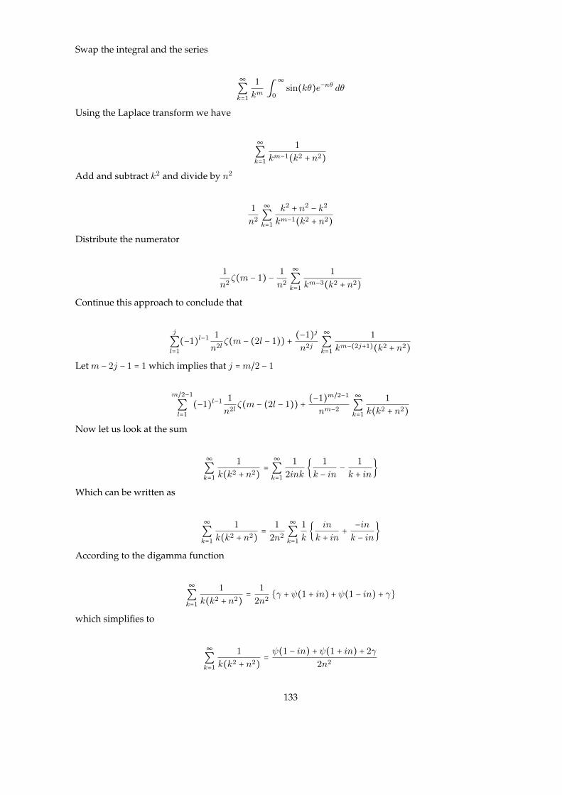
Swap the integral and the series

∞∑k=1

1

km∫

∞

0sin(kθ)e−nθ dθ

Using the Laplace transform we have

∞∑k=1

1

km−1(k2 + n2)

Add and subtract k2 and divide by n2

1

n2

∞∑k=1

k2 + n2 − k2

km−1(k2 + n2)

Distribute the numerator

1

n2ζ(m − 1) − 1

n2

∞∑k=1

1

km−3(k2 + n2)

Continue this approach to conclude that

j

∑l=1

(−1)l−1 1

n2lζ(m − (2l − 1)) + (−1)j

n2j

∞∑k=1

1

km−(2j+1)(k2 + n2)

Let m − 2j − 1 = 1 which implies that j =m/2 − 1

m/2−1

∑l=1

(−1)l−1 1

n2lζ(m − (2l − 1)) + (−1)m/2−1

nm−2

∞∑k=1

1

k(k2 + n2)

Now let us look at the sum

∞∑k=1

1

k(k2 + n2)=

∞∑k=1

1

2ink{ 1

k − in− 1

k + in}


∞∑k=1

1

k(k2 + n2)= 1

2n2

∞∑k=1

1

k{ in

k + in+ −ink − in

}

According to the digamma function

∞∑k=1

1

k(k2 + n2)= 1

2n2{γ + ψ(1 + in) + ψ(1 − in) + γ}

which simplifies to

∞∑k=1

1

k(k2 + n2)= ψ(1 − in) + ψ(1 + in) + 2γ

2n2

133

Now we we can verify ψ(1 − in) = ψ(1 + in)

Which suggests that

ψ(1 + in) + ψ(1 − in) = 2R{ψ(1 + in)}

Hence we have the sum

∞∑k=1

1

k(k2 + n2)= 2R{ψ(1 + in)} + 2γ

2n2= R{ψ(1 + in)} + γ)

n2

This concludes to

m/2−1

∑l=1

(−1)l−1 ζ(m − (2l − 1))n2l

+ (−1)m/2−1R{ψ(1 + in)} + γnm

134

19 Clausen Integral function

19.1 Definiton

We define

cl2(x) = ∑k=1

sin(kx)k2


cl2(θ) = −∫θ

0log [2 sin(φ

2)]dφ

proof


Li2(eiθ) =∞∑k=1

eikθ

k2=

∞∑k=1

cos(kθ)k2

+ i∞∑k=1

sin(kθ)k2

By the integral definition of the dilogarithm

Li2(eiθ) − ζ(2) = −∫eiθ

1

log(1 − x)x

dx

Let x = eiφ

Li2(eiθ) − ζ(2) = −i∫θ

0log(1 − eiφ)dφ

Let us look at the following

1 − eiφ = 1 − cos(φ) − i sin(φ) = 2 sin2(φ/2) − 2i sin(φ/2) cos(φ/2)

Which simplifies to

1 − eiφ = 2 sin(φ/2) [sin(φ/2) − i cos(φ/2)] = 2 sin(φ/2)e−(i/2)(π−φ)

Hence our integral

Li2(eiθ) − ζ(2) = −i∫θ

0log [2 sin(φ/2)e−(i/2)(π−φ)]dφ

Use the complex logarithm properties

Li2(eiθ) − ζ(2) = −i∫θ

0log [2 sin(φ/2)]dφ + 1

4(π − θ)2 − 1

4π2

135

By equating the imaginary parts we have our result.

We can see the special value

cl2 (π2) =

∞∑k=1

sin(kπ/2)k2

=∞∑k=0

(−1)k

(2k + 1)2= G

Where G is the Catalan’s constant.

19.3 Duplication formula

Prove the following

cl2(2θ) = 2(cl2(θ) − cl2(π − θ))

proof

We provide a proof using the integral representation

cl2(2θ) = −∫2θ

0log [2 sin( t

2)]dt

Let t = 2φ

−2∫θ

0log [2 sin (φ)]dφ

Use the double angle identity

−2∫θ

0log [4 sin(φ

2) cos(φ

2)]dφ

Separate the logarithms

−2∫θ

0log [2 sin(φ

2)]dφ − 2∫

θ

0log [2 cos(φ

2)]dφ

We can verify that

cl2(π − θ) = ∫θ

0log [2 cos(φ

2)]dφ

Hence

cl2(2θ) = 2(cl2(θ) − cl2(π − θ))

Using that we get the value

136

cl2(3π) = 2cl2 (3π

2) − 2cl2 (−π

2)

Since cl2(3π) = 0

cl2 (3π

2) = cl2 (−π

2) = −cl2 (π

2) = −G

19.4 Example

Prove that

∫2π

0cl2(x)2dx = π

5

90


∞∑k=1

∞∑n=1

1

(nk)2 ∫2π

0sin(kx) sin(nx)dx

Consider the integral

∫2π

0sin(kx) sin(nx)dx = 1

2∫

2π

0cos((k − n)x) − cos((k + n)x)dx

We have two cases

If n = k then

1

2∫

2π

01 − cos(2nx)dx = π

If n ≠ k

1

2∫

2π

0cos((k − n)x) − cos((k + n)x)dx = 1

2[ sin((k − n)x)

k − n− sin((k + n)x)

k + n]

2π

0

= 0

Hence we have

∫2π

0sin(kx) sin(nx)dx =

⎧⎪⎪⎪⎪⎪⎨⎪⎪⎪⎪⎪⎩

0 n ≠ k

π n = k

We can write the series as

∞∑n=1

∞∑k=1

1

(nk)2=

∞∑n≠k

1

(nk)2+

∞∑n=1

1

n4

Now since the integral n ≠ k goes to zero the result reduces to

137

π∞∑n=1

1

n4= πζ(4) = π

5

90

19.5 Example

Prove that

∫π/2

0x log(sinx) dx = 7

16ζ(3) − π

2

8log 2

proof

I = ∫π2

0x log(sinx)dx = ∫

π2

0x log(2 sinx) − π

2

8log(2)

The integral reduces to

∫π2

0x log(2 sinx)dx = 1

2∫

π2

0Cl2(2θ)dθ

= 1

2∫

π2

0

∞∑n=1

sin(2nθ)n2

dθ

= −1

4∑n=1

(−1)n

n3+ 1

4∑n=1

1

n3

= 7

16ζ(3)

Collecting that together we have

I = 7

16ζ(3) − π

2

8log(2)

19.6 Example

Prove that

∫π/4

0x cot(x)dx = −π

8log(2) +G/2

proof

Start by integration by parts

∫π/4

0x cot(x)dx = π

8log(2) − ∫

π/4

0log(sinx)dx

In the integral

138

∫π/4

0log(sinx)dx

Let x→ t/2

1

2∫

π/2

0log(sin t/2)dt


1

2∫

π/2

0log(2 sin t/2)dt − 1

2∫

π/2

0log(2)dt

Using the Clausen integral function we get

−1

2cl2(π/2) −

π

4log(2)

Note that cl2(π/2) = G

We deduce that

∫π/4

0log(sinx)dx = −G/2 − π

4log(2)


∫π/4

0x cot(x)dx = π

8log(2) +G/2 − π

4log(2) = −π

8log(2) +G/2

19.7 Second Integral representation

Prove that

cl2(θ) = − sin(θ)∫1

0

log(x)x2 − 2 cos(θ)x + 1

dx

proof

Note that

x2 − 2 cos(θ)x + 1 = x2 − (eiθ + e−iθ)x + 1 = (x − eiθ)(x − e−iθ)

This implies

1

x2 − 2 cos(θ)x + 1= 1

eiθ − e−iθ{ 1

x − eiθ− 1

x − e−iθ}

139

Note that eiθ − e−iθ = 2i sin(θ)

1

x2 − 2 cos(θ)x + 1= 1

2i sin(θ){ 1

x − eiθ− 1

x − e−iθ}

Now use the geometric series

1

x2 − 2 cos(θ)x + 1= −1

2i sin(θ){∞∑k=0

xke−i(k+1)θ −∞∑k=0

xkei(k+1)θ}

1

x2 − 2 cos(θ)x + 1= 1

sin(θ)

∞∑k=1

xk−1 sin(kθ)

That implies

− sin(θ)∫1

0

log(x)x2 − 2 cos(θ)x + 1

dx = −∞∑k=1

sin(kθ)∫1

0xk−1 log(x)dx = cl2(θ)

19.8 Example

Find the value of

cl2 (2π

3)

proof

Use the second integral representation

cl2(2π/3) = −√

3

2∫

1

0

log(x)x2 + x + 1

dx

Use that

x3 − 1 = (x − 1)(x2 + x + 1)

Hence

cl2(2π/3) = −√

3

2∫

1

0

x − 1

x3 − 1log(x)dx

Let x3 = t

cl2(2π/3) = −1

6√

3∫

1

0

t1/3−1(t1/3 − 1)t − 1

log(t)dx

Note that

140

ψ′(s) = ∫1

0

xs−1

1 − xlog(x)dx

We deduce that

cl2(2π/3) = −1

6√

3(ψ′(2/3) − ψ′(1/3))

141

20 Barnes G function

20.1 Definition

G(z + 1) = (2π)z/2 exp(−z + z2(1 + γ)2

)∞∏n=1

{(1 + zn)n

exp( z2

2n− z)}

20.1.1 Functional equation

Prove that

G(z + 1) = Γ(z)G(z)

proof

From the series representation we have

G(z + 1)G(z)

=√

2π exp(−z − γz + γ2)

∞∏k=1

( k + zk + z − 1

)k

exp(2z − 1 − 2k

2k) .

This can be written as

G(z + 1)G(z)

= z√

2π exp(−z + γ2)

∞∏k=1

( k + zk + z − 1

)k

exp(−1 + 2k

2k)(1 + z

k) e

−γz

z

∞∏k=1

(1 + zk)−1

e(zk)

Use the definition of the gamma function

G(z + 1)G(z)

= zΓ(z)√

2π exp(−z + γ2)

∞∏k=1

( k + zk + z − 1

)k

exp(−1 + 2k

2k)(1 + z

k)

It suffices to prove that

z√

2π exp(−z + γ2)

∞∏k=1

( k + zk + z − 1

)k

exp(−1 + 2k

2k)(1 + z

k) = 1

or

∞∏k=1

( k + zk + z − 1

)k

exp(−1 + 2k

2k)(1 + z

k) =

exp (z − γ2)

z√

2π

Start by

limN→∞

N

∏k=1

( k + zk + z − 1

)k

exp(−1 + 2k

2k)(1 + z

k)

Notice

142

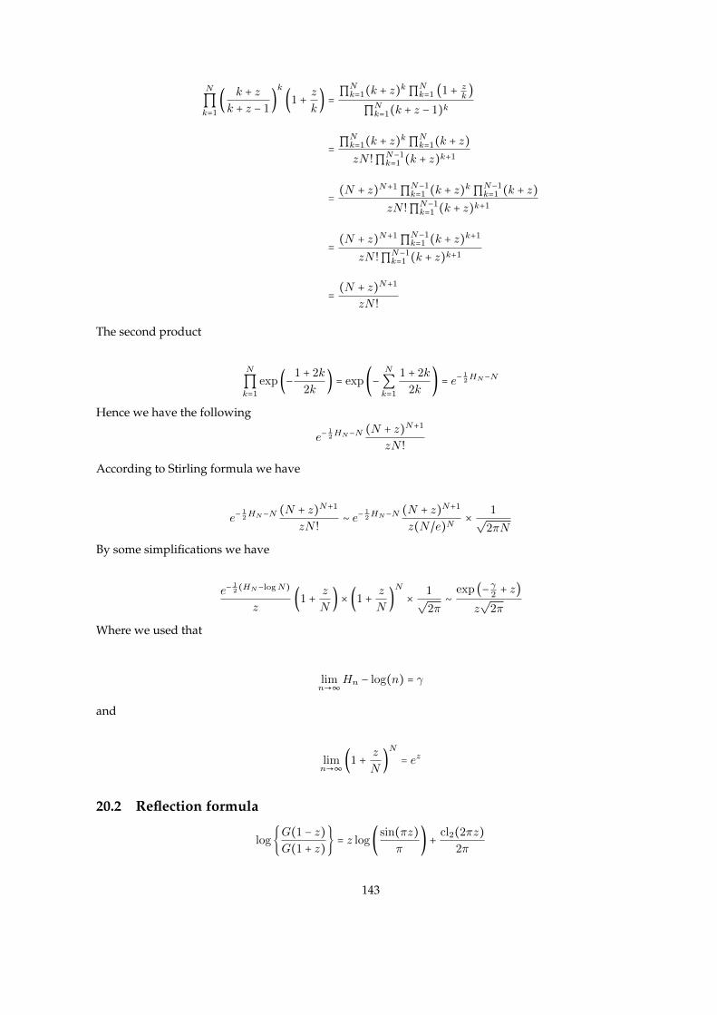
N

∏k=1

( k + zk + z − 1

)k

(1 + zk) =∏Nk=1(k + z)k∏

Nk=1 (1 + z

k)

∏Nk=1(k + z − 1)k

= ∏Nk=1(k + z)k∏

Nk=1(k + z)

zN !∏N−1k=1 (k + z)k+1

= (N + z)N+1∏N−1k=1 (k + z)k∏N−1

k=1 (k + z)zN !∏N−1

k=1 (k + z)k+1

= (N + z)N+1∏N−1k=1 (k + z)k+1

zN !∏N−1k=1 (k + z)k+1

= (N + z)N+1

zN !

The second product

N

∏k=1

exp(−1 + 2k

2k) = exp(−

N

∑k=1

1 + 2k

2k) = e−

12HN−N


e−12HN−N (N + z)N+1

zN !

According to Stirling formula we have

e−12HN−N (N + z)N+1

zN !∼ e−

12HN−N (N + z)N+1

z(N/e)N× 1√

2πN

By some simplifications we have

e−12 (HN−logN)

z(1 + z

N) × (1 + z

N)N

× 1√2π

∼exp (−γ

2+ z)

z√

2π

Where we used that

limn→∞

Hn − log(n) = γ

and

limn→∞

(1 + z

N)N

= ez

20.2 Reflection formula

log{G(1 − z)G(1 + z)

} = z log( sin(πz)π

) + cl2(2πz)2π

143

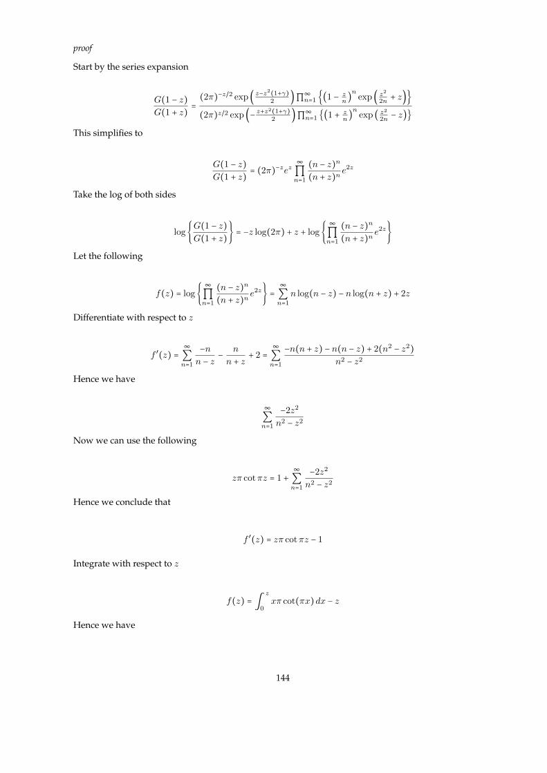
proof

Start by the series expansion

G(1 − z)G(1 + z)

=(2π)−z/2 exp ( z−z

2(1+γ)2

)∏∞n=1 {(1 − z

n)n exp ( z

2

2n+ z)}

(2π)z/2 exp (− z+z2(1+γ)2

)∏∞n=1 {(1 + z

n)n exp ( z2

2n− z)}

This simplifies to

G(1 − z)G(1 + z)

= (2π)−zez∞∏n=1

(n − z)n

(n + z)ne2z

Take the log of both sides

log{G(1 − z)G(1 + z)

} = −z log(2π) + z + log{∞∏n=1

(n − z)n

(n + z)ne2z}

Let the following

f(z) = log{∞∏n=1

(n − z)n

(n + z)ne2z} =

∞∑n=1

n log(n − z) − n log(n + z) + 2z


f ′(z) =∞∑n=1

−nn − z

− n

n + z+ 2 =

∞∑n=1

−n(n + z) − n(n − z) + 2(n2 − z2)n2 − z2

Hence we have

∞∑n=1

−2z2

n2 − z2

Now we can use the following

zπ cotπz = 1 +∞∑n=1

−2z2

n2 − z2


f ′(z) = zπ cotπz − 1

Integrate with respect to z

f(z) = ∫z

0xπ cot(πx)dx − z

Hence we have

144

log{G(1 − z)G(1 + z)

} = −z log(2π) + ∫z

0zπ cot(πx)dx

Now use integration by parts for the integral

∫z

0xπ cot(πx)dx = z log(sinπz) − ∫

z

0log(sinπx)dx (1)

= z log(2 sinπz) − ∫z

0log(2 sinπx)dx (2)

= z log(2 sinπz) − 1

2π∫

2πz

0log (2 sin

x

2)dx (3)

= z log(2 sinπz) + cl2(2πz)2π

(4)

(5)

That implies

log{G(1 − z)G(1 + z)

} = z log(2 sinπz) − z log(2π) + cl2(2πz)2π

= z log( sin(πz)π

) + cl2(2πz)2π

20.3 Values at positive integers

Prove that

G(n) =n−1

∏k=1

Γ(k)

proof

It can be proved by induction. For G(1) = 1, suppose

G(n) =n−1

∏k=1

Γ(k)

We want to show

G(n + 1) =n

∏k=1

Γ(k)

By the functional equation

G(n + 1) = Γ(n)G(n) = Γ(n)n−1

∏k=1

Γ(k) =n

∏k=1

Γ(k)

145

20.4 Relation to Hyperfactorial function

We define the hyperfactorial function as

H(n) =n

∏k=1

kk

Prove for n is a positive integer

G(n + 1) = (n!)n

H(n)

proof

We can prove it by induction for n = 0 we have, G(1) = 1,

suppose that

G(n) = Γ(n)n−1

H(n − 1)

we want to show that

G(n + 1) = Γ(n)G(n) = Γ(n) Γ(n)n−1

H(n − 1)

Notice that

H(n − 1) =n−1

∏ kk = ∏n kk

nn= H(n)

nn

We deduce that

G(n + 1) = Γ(n)G(n) = Γ(n)n × nn

H(n)= (n!)n

H(n)

20.5 Loggamma integral

Prove that

∫z

0log Γ(x)dx = z

2log(2π) + z(z − 1)

2+ z log Γ(z) − logG(z + 1)

proof

Take the log to the series representation

logG(z + 1) = z2

log(2π) − z + z2(1 + γ)2

+∞∑n=1

n log (1 + zn) + z2

2n− z

146

Let the following

f(z) =∞∑n=1

n log (1 + zn) + z2

2n− z


f ′(z) =∞∑n=1

n

z + n+ zn− 1 =

∞∑n=1

z2

n(n + z)

Now use the following

ψ(z) = −γ − 1

z+

∞∑n=1

z

n(n + z)

which implies that

∞∑n=1

z2

n(n + z)= zψ(z) + γz + 1

Hence we have

f ′(z) = zψ(z) + γz + 1

Integrate with respect to z

f(z) = ∫z

0xψ(x)dx + γz

2

2+ z

which implies that

f(z) = z log Γ(z) − ∫z

0log Γ(x)dx + γz

2

2+ z

Hence we have

logG(z + 1) = z2

log(2π) − z + z2(1 + γ)2

+ z log Γ(z) − ∫z

0log Γ(x)dx + γz

2

2+ z

By some rearrangements we have

∫z

0log Γ(x)dx = z

2log(2π) + z(z − 1)


147

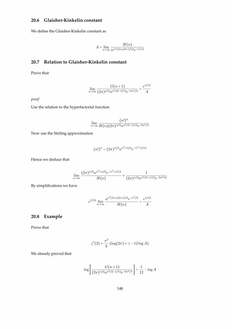
20.6 Glaisher-Kinkelin constant

We define the Glaisher-Kinkelin constant as

A = limn→∞

H(n)nn2/2+n/2+1/12e−n2/4

20.7 Relation to Glaisher-Kinkelin constant

Prove that

limn→∞

G(n + 1)(2π)n/2nn2/2−1/12e−3n2/4 = e

1/12

A

proof

Use the relation to the hyperfactorial function

limn→∞

(n!)n

H(n)(2π)n/2nn2/2−1/12e−3n2/4

Now use the Stirling approximation

(n!)n ∼ (2π)n/2nn2+n/2e−n

2+1/12


limn→∞

(2π)n/2nn2+n/2e−n

2+1/12

H(n)× 1

(2π)n/2nn2/2−1/12e−3n2/4


e1/12 limn→∞

nn2/2+n/2+1/12e−n

2/4

H(n)= e

1/12

A

20.8 Example

Prove that

ζ ′(2) = π2

6(log(2π) + γ − 12 logA)

We already proved that

log [ G(n + 1)(2π)n/2nn2/2−1/12e−3n2/4 ] ∼

1

12− logA

148

Let the following

f(n) = log [ G(n + 1)(2π)n/2nn2/2−1/12e−3n2/4 ]

Use the series representation of the Barnes functions

f(n) = log

⎡⎢⎢⎢⎢⎢⎣

(2π)n/2 exp (−n+n2(1+γ)2

)∏∞k=1 {(1 + n

k)k exp (n

2

2k− n)}

(2π)n/2nn2/2−1/12e−3n2/4

⎤⎥⎥⎥⎥⎥⎦Which reduces to

f(n) = −n + n2(1 + γ)2

+∞∑k=1

{k log (1 + nk) + n

2

2k− n} − (n

2

2− 1

12) log(n) + 3n2

4

Differentiate with respect to n

f ′(n) = −1

2− n − γn + nψ(n) + γn + 1 − n log(n) − n

2+ 1

12n+ 3n

2

Note that we already showed that

d

dn

∞∑k=1

{k log (1 + nk) + n

2

2k− n} = nψ(n) + γn + 1


f ′(n) = nψ(n) − n log(n) + 1

12n+ 1

2

Now use that

ψ(n) = log(n) − 1

2n− 2∫

∞

0

zdz

(n2 + z2)(e2πz − 1)dz


f ′(n) = −2∫∞

0

nzdz

(n2 + z2)(e2πz − 1)dz + 1

12n

Integrate with respect to n

f(n) = −∫∞

0

z log(n2 + z2)(e2πz − 1)

dz + 1

12log(n) +C

Take the limit n→ 0

C = limn→0

f(n) − 1

12log(n) + ∫

∞

0

z log(z2)(e2πz − 1)

dz

149

Hence we have the limit

limn→0

G(n + 1)(2π)n/2nn2/2−1/12e−3n2/4 −

1

12log(n) = lim

n→0log

G(n + 1)(2π)n/2nn2/2e−3n2/4 = 0

Hence we see that

C = 2∫∞

0

z log(z)(e2πz − 1)

dz

Finally we have

f(n) = −∫∞

0

z log(n2 + z2)(e2πz − 1)

dz + 1

12log(n) + 2∫

∞

0


dz

f(n) = −∫∞

0

z log (1 + z2

n2 )(e2πz − 1)

dz − log(n2)∫∞

0

z

(e2πz − 1)dz + 1

12log(n) + 2∫

∞

0


dz

Also we have

∫∞

0

z

(e2πz − 1)dz = 1

24

That simplifies to

f(n) = −∫∞

0

z log (1 + z2

n2 )(e2πz − 1)

dz + 2∫∞

0


dz

Take the limit n→∞

2∫∞

0


dz = 1

12− logA

Now use that

2∫∞

0


dz = 2∫∞

0

z log(z)e2πz

× 1

1 − e−2πzdz

= 2∞∑n=0∫

∞

0e−2πz(n+1)z log(z)dz

=∞∑n=1

ψ(2) − log(2π) + log(n)2π2n2

= (ψ(2) − log(2π))ζ(2) + ζ ′(2)2π2


ζ ′(2) = (log(2π) − ψ(2))ζ(2) + 2π2 ( 1

12− logA) = ζ(2)(log(2π) + γ − 12 logA)

150

20.9 Example

Prove that

ζ ′(−1) = 1

12− logA

proof

Start by

ζ(s) = limm→∞

(m

∑k=1

k−s − m1−s

1 − s− m

−s

2+ sm

−s−1

12) , Re(s) > −3.

Differentiate with respect to s

ζ ′(s) = limm→∞

(−m

∑k=1

k−s log(k) − m1−s

(1 − s)2+ m

1−s

1 − slog(m) + m

−s

2log(m) + m

−s−1

12− m

−s−1

12log(m))

Now let s→ −1

ζ ′(−1) = limm→∞

(−m

∑k=1

k log(k) − m2

4+ m

2

2log(m) + m

2log(m) + 1

12− 1

12log(m))

Take the exponential of both sides

eζ′(−1) = e1/12 lim

m→∞mm2/2+m/2−1/12e−m

2/4

e∑mk=1 k log(k) = e1/12 lim

m→∞mm2/2+m/2−1/12e−m

2/4

H(m)= e

1/12

A

We conclude that

ζ ′(−1) = 1

12− logA

20.10 Relation to Howrtiz zeta function

Prove that

logG(z + 1) − z log Γ(z) = ζ ′(−1) − ζ ′(−1, z)

proof


ζ(s, z) = z−s

2+ z1−s

s − 1+ 2∫

∞

0

sin(sarctan(x/z))(z2 + x2)s/2(e2πx − 1)

dx

Take the derivative with respect to s and s→ −1

151

ζ ′(−1, z) = −z log(z)2

+ z2 log(z)

2− z

2

4+ ∫

∞

0

x log(x2 + z2) + 2z arctan(x/z)(e2πx − 1)

dx

Now use that

ψ(z) = log(z) − 1

2z− 2∫

∞

0

x

(z2 + x2)(e2πx − 1)dx

Which implies that

∫∞

0

2zx

(z2 + x2)(e2πx − 1)dx = z log(z) − 1

2− zψ(z)

By taking the integral

∫∞

0

x log(x2 + z2) − x log(x2)(e2πx − 1)

dx = ∫z

0x log(x)dx − ∫

z

0xψ(x)dx − z

2

Which simplifies to

∫∞

0

x log(x2 + z2)(e2πx − 1)

dx = ζ ′(−1) − z2

4+ 1

2z2 log(z) − z log Γ(z) + ∫

z

0log Γ(x)dx − z

2

Also we have

2∫∞

0

x

(x2 + z2)(e2πx − 1)dx = log(z) − 1

2z− ψ(z)

By integration we have

2∫∞

0

arctan(x/z)(e2πx − 1)

dx = z + log(z)2

− z log(z) + log Γ(z) +C

Let z → 1 to evaluate the constant

2∫∞

0

arctan(x/z)(e2πx − 1)

dx = z + log(z)2

− z log(z) + log Γ(z) − 1

2log(2π)

Multiply by z

2∫∞

0

z arctan(x/z)(e2πx − 1)

dx = z2 + z log(z)2

− z2 log(z) + z log Γ(z) − z2

log(2π)

Substitute both integrals in our formula

∫z

0log Γ(x)dx = z

2log(2π) + z(1 − z)

2− ζ

′

(−1) + ζ′

(−1, z)

We also showed that

152

∫z

0log Γ(x)dx = z

2log(2π) + z(1 − z)


By equating the equations we get our result.

20.11 Example

Prove that

G(1

2) = 21/24π−1/4e1/8A−3/2

proof

We know that

logG(z) + log Γ(z) − z log Γ(z) = ζ ′(−1) − ζ ′(−1, z)

Note that

ζ (s, 1

2) = (2s − 1)ζ(s)

Which implies that

ζ ′ (−1,1

2) = log(2)

2ζ(−1) − 1

2ζ ′(−1)

Hence we have

logG(1

2) + 1

2log Γ(1

2) = 3

2ζ ′(−1) − log(2)

2ζ(−1)

Using that we have

G(1

2) = 21/24π−1/4e

32 ζ

′(−1)

Note that

ζ(−1) = − 1

12

This can be proved by the functional equation of the zeta function.

153

References

[1] Leonard Lewin. Polylogarithms and associated functions. New York, 1981.

[2] Marko Petkovsek, Herbert Wilf, Dorom Zeilbegreger. A=B. Philadelphia, 1997.

[3] Pedro Freitas. Integrals of polylogarithmic functions, recurrence relations and associated Euler sums. 2004.

[4] Gradshteyn, Ryhik. Edited by Alan Jeffrey, Daniel Zillinger. Table of integrals, series and products. 2007.

[5] Habib Muzaffiar, Kenneth Williams. Evaluation of complete elleptic integrals of the first kind at singular

moduli. 2006.

[6] Stefan Boettner, Victor Moll. The integrals in Gradshteyn and Ryzhik, Part 16: Complete elliptic integrals.

2010.

[7] Factorial, Gamma and Beta function http://mhtlab.uwaterloo.ca/courses/me755/web_chap1.pdf

[8] Keith Conrad. Differentiation under the integral sign.

[9] http://www.mymathforum.com

[10] http://www.mathhelpboards.com

[11] http://www.mathstackexchange.com

[12] http://www.integralsandseries.prophpbb.com

[13] http://www.wikipedia.org

[14] http://mathworld.wolfram.com

[15] http://dlmf.nist.gov/

154

Advanced Integration Techniques - WordPress.comAdvanced Integration Techniques Advanced approaches...

Documents

Transcript of Advanced Integration Techniques - WordPress.comAdvanced Integration Techniques Advanced approaches...