Advanced Digital Signal Processing Based Redefined Power ... · ADVANCED DIGITAL SIGNAL PROCESSING...
137
University of South Carolina Scholar Commons eses and Dissertations 12-15-2014 Advanced Digital Signal Processing Based Redefined Power Quality Indices, and eir Applications to Wind Power Md Moinul Islam University of South Carolina - Columbia Follow this and additional works at: hp://scholarcommons.sc.edu/etd is Open Access Dissertation is brought to you for free and open access by Scholar Commons. It has been accepted for inclusion in eses and Dissertations by an authorized administrator of Scholar Commons. For more information, please contact [email protected]. Recommended Citation Islam, M. M.(2014). Advanced Digital Signal Processing Based Redefined Power Quality Indices, and eir Applications to Wind Power. (Doctoral dissertation). Retrieved from hp://scholarcommons.sc.edu/etd/2987
Transcript of Advanced Digital Signal Processing Based Redefined Power ... · ADVANCED DIGITAL SIGNAL PROCESSING...

University of South CarolinaScholar Commons
Theses and Dissertations
12-15-2014
Advanced Digital Signal Processing BasedRedefined Power Quality Indices, and TheirApplications to Wind PowerMd Moinul IslamUniversity of South Carolina - Columbia
Follow this and additional works at: http://scholarcommons.sc.edu/etd
This Open Access Dissertation is brought to you for free and open access by Scholar Commons. It has been accepted for inclusion in Theses andDissertations by an authorized administrator of Scholar Commons. For more information, please contact [email protected].
Recommended CitationIslam, M. M.(2014). Advanced Digital Signal Processing Based Redefined Power Quality Indices, and Their Applications to Wind Power.(Doctoral dissertation). Retrieved from http://scholarcommons.sc.edu/etd/2987

ADVANCED DIGITAL SIGNAL PROCESSING BASED REDEFINED POWER QUALITY
INDICES, AND THEIR APPLICATIONS TO WIND POWER
by
Md Moinul Islam
Bachelor of Science
Bangladesh University of Engineering and Technology, 2007
Master of Engineering
University of South Carolina, 2011
Submitted in Partial Fulfillment of the Requirements
for the Degree of Doctor of Philosophy in
Electrical Engineering
College of Engineering and Computing
University of South Carolina
2014
Accepted by:
Charles Brice, Major Professor
Enrico Santi, Committee Member
Herbert Ginn, Committee Member
Lingyu Yu, Committee Member
Lacy Ford, Vice Provost and Dean of Graduate Studies

c© Copyright by Md Moinul Islam, 2014
All Rights Reserved.
ii

DEDICATION
Dedicated to my wife Navila Rahman, my newborn baby Maahira Islam, my late par-
ents Md Nazrul Islam, and Shirin Akter, and my step mother Shahina Akter.
iii

ACKNOWLEDGMENTS
I would like to thank all of those who contributed their valuable times to help me. A spe-
cial thanks goes to my academic adviser Dr. Charles Brice who helped me in the strenuous
process of my graduation, successful completion of research projects, finishing this dis-
sertation document, and his continuous support to stay focus. I would like to thank Dr.
Yong-June Shin as well for teaching me time-frequency analysis technique, and his time
for my research publications, and for the support during his stay in the US. Dr. Roger Dou-
gal and Dr. Enrico Santi also helped me through attending my practice presentations for
GRid-connected Advanced Power Electronics Systems (GRAPES) center, and with their
valuable guidelines and suggestions to make successful presentations and completion of
the projects. I would like to thank Dr. Herbert Ginn and Dr. Lingyu Yu for attending my
final defense. I would also like to thank Nat Paterson, Burt Ashley, and Hope Johnson
for their time and efforts for helping me with official procedures for my dissertation, and
research trips. I would like to thank Rich Smart as well for helping me writing my research
publications.
I would like to thank the members of the Power IT group in South Carolina. I would
like to thank Dr. Phillip E. C. Stone for helping me out in the beginning of my graduate re-
search. I would also like to thank my collaborators Hossein Ali Mohammadpur and Cuong
Nguyen for their help and contributions in the successful completion of the projects in a
team-environment. Wang Jing-Jang, Mohammed Hassan, Patrick Mitchell, Ryan Lukens,
Amin Ghaderi, and Qiu Deng were all members of the same research team, and gave me
helpful advice and suggestions throughout my studies. Last, but not least, I would like to
thank all of my family and close friends who sacrificed time for me: my wife Navila Rah-
iv

man, my mother Shahina Akter, my siblings Mrs. Rahima Akter, Md Ziaul Islam, Fatema
Akter, my uncle Md Monirul Islam, my friends Rassel Raihan, Iftekhar Hossain Shovon,
B. M. Farid Rahman, Fazle Rabbi, Sayful Islam, Atikur Rahman, Faisal Jahan, and Ishtiaq
Rouf who always supported me, and helped me focus. I would also like to thank all the
Bangladeshi faculty members and the rest of the Bangladeshi community in Columbia, SC
for wonderful times on different social, religious, and cultural occasions.
The projects that make up this dissertation document have been supported by Indus-
try/University Cooperative Research Center on GRid-connected Advanced Power Elec-
tronics Systems (GRAPES) center. I would like to thank all the IAB members, especially
Dr. Ram Adapa, involved in the GRAPES for their comments, and suggestions for success-
ful completion of all the projects. Thanks to NREL and AEP for providing us real-world
power quality disturbances that which have been utilized in my dissertation for analysis
purpose.
v

ABSTRACT
This dissertation proposes a time-frequency distribution (TFD) based new method to rede-
fine the power quality (PQ) indices for the assessment of PQ disturbances typically present
in electric power systems. The redefined PQ indices are applied to various types of syn-
thetic and real-world PQ disturbances in order to verify the efficacy and applicability of
the proposed method. The case studies show that the proposed method provides actual re-
sults with respect to the existing TFD-based transient PQ indices, and provides much more
accurate results than the traditional fast Fourier transform (FFT) based PQ indices under
stationary and nonstationary PQ disturbances.
In addition, utilizing the proposed method, the power components contained in the
IEEE Standard 1459-2010 are redefined for single-phase, and three-phase power systems
under sinusoidal, nonsinusoidal, balanced and unbalanced conditions. Unlike the tradi-
tional FFT-based method, the proposed method is able to extract the time information lost
in the FFT, and provides very accurate and instantaneous assessment of the power com-
ponents according to the IEEE Standard 1459-2010. Also, the proposed method will have
the advantage of finding the instantaneous direction of time-varying harmonics power flow
which can be positive or negative depending on the harmonics flow to the network or to
the load. According to the IEEE Standard 1459-2010, the harmonic active power PH is
obtained by subtracting the fundamental active power P1 from the total active power P
(PH = P− P1). However, the indirect measurement of the harmonic active power may
provide imprecise result since harmonic active power is generally very small part of the
total active power. In this dissertation, a direct assessment of the harmonic active power is
carried out to obtain accurate result based on the proposed method.
vi

In addition, a new perspective for wind power grid codes is proposed in order to verify
that a wind generating plant conforms to grid codes requirements under stationary and non-
stationary PQ disturbances, and to obtain supervisory data to protect system reliability.
The proposed method is also able to extract the dynamic signature of PQ disturbances
introduced by variable speed wind energy conversion systems onto the electrical grid. Also,
a TFD-based new method is proposed for the assessment of grid frequency deviation caused
by wind power fluctuations in fixed speed wind energy conversion systems.
vii

TABLE OF CONTENTS
DEDICATION . . . . . . . . . . . . . . . . . . . . . . . . . . . . . . . . . . . iii
ACKNOWLEDGMENTS . . . . . . . . . . . . . . . . . . . . . . . . . . . . . . iv
ABSTRACT . . . . . . . . . . . . . . . . . . . . . . . . . . . . . . . . . . . . vi
LIST OF TABLES . . . . . . . . . . . . . . . . . . . . . . . . . . . . . . . . . xi
LIST OF FIGURES . . . . . . . . . . . . . . . . . . . . . . . . . . . . . . . . xii
CHAPTER 1 INTRODUCTION . . . . . . . . . . . . . . . . . . . . . . . . . . 1
1.1 Motivation and Objectives . . . . . . . . . . . . . . . . . . . . . . . . . . 1
1.2 Organization . . . . . . . . . . . . . . . . . . . . . . . . . . . . . . . . . . 8
CHAPTER 2 TIME-FREQUENCY DISTRIBUTION, AND ITS ISSUES IN DEFIN-
ING POWER QUALITY INDICES . . . . . . . . . . . . . . . . . . 10
2.1 Time-Frequency Distribution . . . . . . . . . . . . . . . . . . . . . . . . . 10
2.2 Issues Associated with TFD in Defining PQ Indices . . . . . . . . . . . . . 13
CHAPTER 3 POWER QUALITY ANALYSIS OF VARIABLE SPEED TURBINE
GENERATORS . . . . . . . . . . . . . . . . . . . . . . . . . . . 21
3.1 Review of Existing RID-Based PQ Indices . . . . . . . . . . . . . . . . . . 21
3.2 Power Quality of Wind Power . . . . . . . . . . . . . . . . . . . . . . . . 23
3.3 Wind Energy Conversion System . . . . . . . . . . . . . . . . . . . . . . . 24
3.4 IEC PQ Standards . . . . . . . . . . . . . . . . . . . . . . . . . . . . . . . 26
3.5 PQ Analysis of wind turbine DFIG and SG . . . . . . . . . . . . . . . . . . 27
viii

3.6 Conclusion . . . . . . . . . . . . . . . . . . . . . . . . . . . . . . . . . . 34
CHAPTER 4 ASSESSMENT OF FUNDAMENTAL FREQUENCY DEVIATION OF
FIXED SPEED WIND ENERGY CONVERSION SYSTEM . . . . . . . 35
4.1 Introduction . . . . . . . . . . . . . . . . . . . . . . . . . . . . . . . . . . 35
4.2 Studied Wind Energy Conversion System . . . . . . . . . . . . . . . . . . 36
4.3 Case Studies . . . . . . . . . . . . . . . . . . . . . . . . . . . . . . . . . . 38
4.4 Conclusion . . . . . . . . . . . . . . . . . . . . . . . . . . . . . . . . . . 46
CHAPTER 5 REDEFINED EXISTING REDUCED INTERFERENCE DISTRIBU-
TION BASED POWER QUALITY INDICES FOR STATIONARY AND
NONSTATIONARY POWER QUALITY DISTURBANCES . . . . . . . 47
5.1 Introduction . . . . . . . . . . . . . . . . . . . . . . . . . . . . . . . . . . 47
5.2 Limitations of Existing Transient PQ Indices . . . . . . . . . . . . . . . . . 47
5.3 Redefined PQ Indices . . . . . . . . . . . . . . . . . . . . . . . . . . . . . 49
5.4 Case Study Analysis . . . . . . . . . . . . . . . . . . . . . . . . . . . . . . 53
5.5 Conclusion . . . . . . . . . . . . . . . . . . . . . . . . . . . . . . . . . . 60
CHAPTER 6 SINGLE-PHASE INSTANTANEOUS POWER COMPONENTS FOR
TRANSIENT DISTURBANCES ACCORDING TO THE IEEE STAN-
DARD 1459-2010 . . . . . . . . . . . . . . . . . . . . . . . . . 63
6.1 Introduction . . . . . . . . . . . . . . . . . . . . . . . . . . . . . . . . . . 63
6.2 Definitions of Power Components . . . . . . . . . . . . . . . . . . . . . . 63
6.3 Redefined Power Components . . . . . . . . . . . . . . . . . . . . . . . . 65
6.4 Case Study Analysis . . . . . . . . . . . . . . . . . . . . . . . . . . . . . . 68
6.5 Conclusion . . . . . . . . . . . . . . . . . . . . . . . . . . . . . . . . . . 78
ix

CHAPTER 7 REDEFINED THREE-PHASE POWER COMPONENTS ACCORD-
ING TO IEEE STANDARD 1459-2010 UNDER NONSINUSOIDAL,
BALANCED AND UNBALANCED CONDITIONS . . . . . . . . . . . 79
7.1 Introduction . . . . . . . . . . . . . . . . . . . . . . . . . . . . . . . . . . 79
7.2 Review of Three-Phase Power Components . . . . . . . . . . . . . . . . . 79
7.3 Redefined Three-Phase Power Components . . . . . . . . . . . . . . . . . 82
7.4 PQ Disturbance Case Study Analysis . . . . . . . . . . . . . . . . . . . . . 85
7.5 Conclusion . . . . . . . . . . . . . . . . . . . . . . . . . . . . . . . . . . 89
CHAPTER 8 A NEW PERSPECTIVE FOR WIND POWER GRID CODES UNDER
POWER QUALITY DISTURBANCES . . . . . . . . . . . . . . . . 91
8.1 Introduction . . . . . . . . . . . . . . . . . . . . . . . . . . . . . . . . . . 91
8.2 Power Quality Indices for Wind Power Grid Codes . . . . . . . . . . . . . 94
8.3 Simulated Case Study . . . . . . . . . . . . . . . . . . . . . . . . . . . . . 97
8.4 Studied Wind Generating Plant . . . . . . . . . . . . . . . . . . . . . . . . 98
8.5 Conclusion . . . . . . . . . . . . . . . . . . . . . . . . . . . . . . . . . . 106
CHAPTER 9 CONCLUSION . . . . . . . . . . . . . . . . . . . . . . . . . . . 107
BIBLIOGRAPHY . . . . . . . . . . . . . . . . . . . . . . . . . . . . . . . . . 109
x

LIST OF TABLES
Table 2.1 Kernels of Cohen’s class TFDs . . . . . . . . . . . . . . . . . . . . . . . 12
Table 3.1 PQ indices for transient disturbance . . . . . . . . . . . . . . . . . . . . 33
Table 3.2 PQ indices for three-phase-to-ground fault . . . . . . . . . . . . . . . . . 34
Table 4.1 Parameters of single 0.746 MW and aggregated 100 MW Fixed Speed
wind energy conversion system . . . . . . . . . . . . . . . . . . . . . . 38
Table 4.2 Ramp and Gust Wind Speed Data . . . . . . . . . . . . . . . . . . . . . 38
Table 4.3 Random Wind Speed Data . . . . . . . . . . . . . . . . . . . . . . . . . 39
Table 5.1 Power Quality Analysis Results (pu) for Stationary Example . . . . . . . 55
Table 5.2 Power Quality Analysis Results (pu) for Transient Example . . . . . . . 57
Table 5.3 PQ Analysis Results (pu) for Voltage Swell Example . . . . . . . . . . . 59
Table 5.4 PQ Analysis Results (pu) for Voltage Sag Example . . . . . . . . . . . . 61
Table 6.1 Stationary Case Study Results . . . . . . . . . . . . . . . . . . . . . . . 69
Table 7.1 Three-Phase Power Components in pu Obtained via various TFDs for
Stationary PQ Disturbance case study (Sbase = 100 kVA, Vbase = 380 V) . 86
Table 7.2 Three-Phase Power Components in pu Obtained via various TFDs for
nonstationary PQ disturbance case study (Sbase = 100 kVA, Vbase =
380 V) . . . . . . . . . . . . . . . . . . . . . . . . . . . . . . . . . . . 88
Table 8.1 Summary of Case Study Analysis Results . . . . . . . . . . . . . . . . . 105
xi

LIST OF FIGURES
Figure 1.1 A nonstationary PQ disturbance signal comprised of 60 Hz, 7th, and
time-varying 15th harmonic components. . . . . . . . . . . . . . . . . . 2
Figure 1.2 FFT of the nonstationary PQ disturbance signal. . . . . . . . . . . . . . 2
Figure 1.3 Time-frequency distribution of the nonstationary PQ disturbance
signal in Fig. 1.1 . . . . . . . . . . . . . . . . . . . . . . . . . . . . . . 4
Figure 2.1 (a) A transient PQ disturbance. . . . . . . . . . . . . . . . . . . . . . . 14
Figure 2.2 TFD of the transient signal utilizing (a) WV TFD, and (b) RID TFD. . . 15
Figure 2.3 Transient PQ voltage and current disturbances. . . . . . . . . . . . . . . 16
Figure 2.4 (a) Active power P, (b) Reactive power Q, and (c) Apparent power
S obtained via RID. . . . . . . . . . . . . . . . . . . . . . . . . . . . . 17
Figure 2.5 Active power of the voltage and current PQ disturbances utilizing
(a) WV TFD, and (b) RID TFD . . . . . . . . . . . . . . . . . . . . . . 18
Figure 2.6 Computational time associated with WV, CW, RID, and Page TFDs
with an increase number of inputs. . . . . . . . . . . . . . . . . . . . . 19
Figure 3.1 Block diagram of a variable speed (a) Wind turbine DFIG and, (b)
Wind turbine SG. . . . . . . . . . . . . . . . . . . . . . . . . . . . . . 25
Figure 3.2 Instantaneous voltage, extracted disturbance, and time-frequency
distribution of the disturbance due to introduction of a wind turbine
DFIG. . . . . . . . . . . . . . . . . . . . . . . . . . . . . . . . . . . . 27
Figure 3.3 PCC RMS voltage of (a) WTG DFIG and (b) WTG SG for generator trip. 28
Figure 3.4 Instantaneous voltage, extracted disturbance, and time-frequency
distribution of the disturbance introduced by wind turbine DFIG trip. . . 29
xii

Figure 3.5 Instantaneous voltage, extracted disturbance, and time-frequency
distribution of the disturbance introduced by wind turbine SG trip. . . . 29
Figure 3.6 (a) Instantaneous THD (ITHD(t)) and (b) Instantaneous frequency
(IF(t)) for wind turbine DFIG trip. . . . . . . . . . . . . . . . . . . . . 30
Figure 3.7 (a) Instantaneous THD (ITHD(t)) and (b) Instantaneous frequency
(IF(t)) respectively for wind turbine SG trip. . . . . . . . . . . . . . . . 30
Figure 3.8 PCC RMS voltage of (a) Wind turbine DFIG and (b) wind turbine
SG for a three phase line-to-ground fault. . . . . . . . . . . . . . . . . . 31
Figure 3.9 Instantaneous voltage, extracted disturbance, and time-frequency
distribution of the disturbance introduced by a three-phase-to-ground
fault applied to a wind turbine DFIG. . . . . . . . . . . . . . . . . . . . 31
Figure 3.10 Instantaneous voltage, extracted disturbance, and time-frequency
distribution of the disturbance introduced by a three-phase-to-ground
fault applied to wind turbine SG. . . . . . . . . . . . . . . . . . . . . . 32
Figure 3.11 (a) Instantaneous THD (ITHD(t)), and (b) Instantaneous frequency
(IF(t)) for a fault applied to a wind turbine DFIG. . . . . . . . . . . . . 32
Figure 3.12 (a) Instantaneous THD (ITHD(t)) and (b) Instantaneous frequency
(IF(t)) for a fault applied to wind turbine SG. . . . . . . . . . . . . . . . 33
Figure 4.1 One line diagram of a fixed speed wind energy conversion system. . . . 37
Figure 4.2 (a) Ramp wind speed, (b) Rotor speed, (c) Power delivered to the
grid, and (d) Grid current signal. . . . . . . . . . . . . . . . . . . . . . 40
Figure 4.3 TFD of the grid current signal. . . . . . . . . . . . . . . . . . . . . . . 41
Figure 4.4 Instantaneous frequency of the grid current signal. . . . . . . . . . . . . 41
Figure 4.5 (a) Ramp wind speed, (b) Rotor speed, (c) Power delivered to the
grid, and (d) Grid current signal. . . . . . . . . . . . . . . . . . . . . . 42
Figure 4.6 TFD of the grid current signal. . . . . . . . . . . . . . . . . . . . . . . 43
Figure 4.7 Instantaneous frequency of the grid current signal. . . . . . . . . . . . . 43
xiii

Figure 4.8 (a) Random wind speed, (b) Rotor speed, (c) Power delivered to the
grid, and (d) Grid current signal. . . . . . . . . . . . . . . . . . . . . . 44
Figure 4.9 TFD of the grid current signal. . . . . . . . . . . . . . . . . . . . . . . 45
Figure 4.10 Instantaneous frequency of the grid current signal. . . . . . . . . . . . . 45
Figure 5.1 Transient PQ indices (a) ITHD, (b) IDIN, (c) IF, and (d) IK accord-
ing to the [22]. . . . . . . . . . . . . . . . . . . . . . . . . . . . . . . . 49
Figure 5.2 (a) Voltage THD, (b) Voltage DIN, (c) PF, (d) Voltage TIF, and (e)
Voltage K-factor for stationary PQ disturbance. . . . . . . . . . . . . . 54
Figure 5.3 A transient PQ (a) Voltage, and (b) Current disturbance waveforms. . . . 55
Figure 5.4 (a) Voltage THD, (b) Voltage DIN, (c) PF, (d) Voltage TIF, and (e)
Voltage K-factor for transient PQ disturbance. . . . . . . . . . . . . . . 56
Figure 5.5 A (a) Voltage swell, and corresponding (b) Current PQ disturbance
waveforms. . . . . . . . . . . . . . . . . . . . . . . . . . . . . . . . . 57
Figure 5.6 (a) Voltage THD, (b) Voltage DIN, (c) PF, (d) Voltage TIF, and (e)
Voltage K-factor for voltage swell PQ disturbance. . . . . . . . . . . . . 58
Figure 5.7 A (a) Voltage sag, and corresponding (b) Current disturbance waveforms 59
Figure 5.8 (a) Voltage THD, (b) Voltage DIN, (c) PF, (d) Voltage TIF, and (e)
Voltage K-factor for voltage sag PQ disturbance. . . . . . . . . . . . . . 60
Figure 6.1 TF based fundamental (a) Active power, (b) Reactive power, and
non-fundamental (c) Active power and (d) Reactive power spectra
of the steady state signal, respectively. . . . . . . . . . . . . . . . . . . 68
Figure 6.2 TF based fundamental and non-fundamental active power and reac-
tive power spectra of the transient disturbance signal. . . . . . . . . . . 70
Figure 6.3 TF based fundamental power components of the transient distur-
bance signal. . . . . . . . . . . . . . . . . . . . . . . . . . . . . . . . . 70
xiv
Figure 6.4 Instantaneous non-fundamental and combined power components
of the transient disturbance signal. . . . . . . . . . . . . . . . . . . . . 71
Figure 6.5 Capacitor switching (a) Voltage waveform, (b) Current waveform,
separated (c) Fundamental voltage, (d) Fundamental current, (e)
Voltage disturbance, and (f) Current disturbance, respectively. . . . . . . 73
Figure 6.6 TF based fundamental and non-fundamental active power and reac-
tive power spectra of the real-world transient disturbance case study. . . 73
Figure 6.7 Time-frequency distribution of transient voltage disturbance. . . . . . . 74
Figure 6.8 Time-frequency distribution of transient current disturbance. . . . . . . 74
Figure 6.9 Disturbance active power in time-frequency domain obtained via XTFD. 75
Figure 6.10 Instantaneous fundamental power components of the real-world tran-
sient disturbance case study. . . . . . . . . . . . . . . . . . . . . . . . . 75
Figure 6.11 Instantaneous non-fundamental and combined power components
of the real-world transient disturbance case study. . . . . . . . . . . . . 76
Figure 7.1 A steady state, nonsinusoidal and unbalanced PQ (a) Voltage, and
(b) Current disturbance waveforms . . . . . . . . . . . . . . . . . . . . 85
Figure 7.2 Percentage errors associated with various TFDs for three-phase sta-
tionary PQ disturbance case study . . . . . . . . . . . . . . . . . . . . . 87
Figure 7.3 Three-phase nonstationary PQ disturbance-(a) Voltage sag, and cor-
responding (b) Current disturbance waveforms . . . . . . . . . . . . . . 87
Figure 7.4 Percentage errors associated with various TFDs for three-phase volt-
age sag case study . . . . . . . . . . . . . . . . . . . . . . . . . . . . . 89
Figure 8.1 Low voltage ride through curve by FERC. . . . . . . . . . . . . . . . . 92
Figure 8.2 Percentage errors associated with the simulated state case study analysis. 97
Figure 8.3 Simplified one-line diagram of Trent Mesa wind project. . . . . . . . . . 98
Figure 8.4 (a) Voltage sag, and (b) Current disturbance waveforms. . . . . . . . . . 99
xv

Figure 8.5 Results of voltage sag case study analysis - Effective (a1) rms volt-
age, (a2) power Factor, (a3) Voltage THD, (a4) Current THD, (b1)
Positive sequence active power, (b2) Harmonic active power, (b3)
Total active power, (b4) Harmonic apparent power, (c1) Non-fundametnal
apparent power, (c2) Total apparent power, (c3) Positive sequence
reactive power, and (c4) Harmonic pollution factor. . . . . . . . . . . . 100
Figure 8.6 Transient (a) Voltage, and (b) Current disturbance waveforms. . . . . . . 101
Figure 8.7 Results of trasient case study analysis - Effective (a1) rms voltage,
(a2) power Factor, (a3) Voltage THD, (a4) Current THD, (b1) Pos-
itive sequence active power, (b2) Harmonic active power, (b3) Total
active power, (b4) Harmonic apparent power, (c1) Non-fundametnal
apparent power, (c2) Total apparent power, (c3) Positive sequence
reactive power, and (c4) Harmonic pollution factor. . . . . . . . . . . . 102
Figure 8.8 Oscillatory (a) Voltage, and (b) Current disturbance waveforms. . . . . . 103
Figure 8.9 Results of oscillatory case study analysis - Effective (a1) rms volt-
age, (a2) power Factor, (a3) Voltage THD, (a4) Current THD, (b1)
Positive sequence active power, (b2) Harmonic active power, (b3)
Total active power, (b4) Harmonic apparent power, (c1) Non-fundametnal
apparent power, (c2) Total apparent power, (c3) Positive sequence
reactive power, and (c4) Harmonic pollution factor. . . . . . . . . . . . 104
xvi

CHAPTER 1
INTRODUCTION
1.1 MOTIVATION AND OBJECTIVES
The increase penetration of nonlinear loads and power electronic devices such as dis-
tributed generation, variable frequency drives, electric arc furnaces, and flexible ac trans-
mission systems in the existing grid are sources of low electric power quality (PQ) [1]-[7].
Low electric PQ encompasses the loss of 10 billion Euros in Europe, and U.S. 24 billion
every year [8]. For assessment purpose of the electric power degradation, PQ indices such
as total harmonic distortion (THD), distortion index (DIN), power factor (PF), telephone
interference factor (TIF), C message, and K-factor are defined in [9]. The IEEE 519 [10]
and IEC 61400-21 [11] are also two examples for the assessment of low electric PQ in
electric power systems. The most recommended power theory for the assessment of low
electric PQ can be found in IEEE Standard 1459 [12], [13] that defines a set of power com-
ponents such as displacement power factor, distortion power, harmonic pollution, and total
power factor for single-phase, and three-phase electrical power systems under sinusoidal,
nonsinusoidal, balanced or unbalanced conditions.
According to the IEEE Standard 1459, the PQ indices are defined based on the “fre-
quency domain” approach utilizing the fast Fourier transform (FFT). The application of the
FFT in defining the power components according to the IEEE Standard 1459 is employed
for single-phase and three-phase electrical power systems in [14], [15], respectively. How-
ever, FFT inherently assumes the signal is periodic, therefore, it can provide accurate re-
sults in case of stationary PQ disturbances only. In fact, not all real-world PQ disturbances
1

0 0.03 0.07 0.1−3
0
3
PQ
Dis
turb
ance
Sig
nal (
pu)
Time (s)
Figure 1.1: A nonstationary PQ disturbance signal comprised of 60 Hz, 7th, and time-
varying 15th harmonic components.
0.06 0.42 0.9 1.50
0.4
0.8
1
Frequency (kHz)
Am
plitu
de (
pu)
Figure 1.2: FFT of the nonstationary PQ disturbance signal.
such as voltage sag, voltage swell, capacitor switching, etc. result in periodic waveform
and exhibit time-varying harmonics characteristics, and can be best described as nonsta-
tionary in nature. Therefore, FFT-based method provides erroneous assessment of the PQ
indices in the presence of PQ disturbances typically present in electrical power systems
due to spectral leakage [16]-[25]. In addition, no time information can be obtained via
FFT since the power components are evaluated in the frequency domain. For example,
Fig. 1.1 represents a nonstationary PQ disturbance signal which is composed of 60 Hz,
7th harmonic, and time-varying 15th harmonic that persists from 0.03 to 0.07 s. The cor-
responding FFT in Fig. 1.2 confirms that the PQ disturbance signal is comprised of 60 Hz,
7th, and 15th harmonic components, however, it does not provide any time information
regarding the presence of these frequency components in the PQ disturbance signal. Also,
side lobes are observed in Fig. 1.2 at other frequency components rather than 60 Hz, 7th,
and 15th harmonic components due to spectral leakage phenomenon that causes inaccurate
2

assessment of nonstationary PQ disturbances.
Regarding the limitations of the FFT, “time domain” techniques based on the Clarke-
Park transformation have been utilized for the measurement purpose of the power compo-
nents in [26]-[31]. The approaches in [29]-[31] are particularly more convenient than the
frequency domain technique for the measurement of the power components according to
the IEEE Standard 1459 as one can assess the fundamental and positive-sequence compo-
nents of voltage and current without any spectral analysis. Nonetheless, the assessment of
the power components under nonsinusoidal conditions may be erroneous because of the
low-pass filters employed in the methods [32]. It has been illustrated in [32] that in order
to obtain more accurate results using the methods in [29]-[31], high order filters with spe-
cific cut-off frequencies must be employed depending on the grid conditions. Therefore,
low-pass filters are replaced in [32] with a recursive algorithm which estimates the aver-
age values. The method shows improved assessment precision, however, it suffers from
synchronization restrictions for frequency excursions as does the FFT [33].
“Time-frequency domain” is another viable alternative approach for the analysis of
PQ disturbances as it can preserve simultaneous time and variable harmonics information
of nonstationary PQ disturbance events. One of the time-frequency domain techniques
based on wavelet transform has been frequently utilized in assessment, detection, localiza-
tion, and classification of nonstationary PQ disturbances in [34]-[39]. Also, Morsi et al.
redefined the single-phase and three-phase power components in time-frequency domain
according to the IEEE Standard 1459 employing discrete wavelet transform, stationary
wavelet transform, and wavelet packet transform in [17]-[21], which acquire very accurate
results for different types of stationary and nonstationary PQ disturbance events. However,
wavelet transform employs long window for low frequency components, and short win-
dow for high frequency components, respectively. Therefore, good frequency resolution
but low time resolution are obtained for the low frequency components, and good time
resolution but low frequency resolution are acquired for the high frequency components
3

Time−Frequency Distribution of a PQ Disturbance Signal
Time (s)
Fre
quen
cy (
kHz)
0 0.03 0.07 0.1
0.06
0.42
0.9
1.5
1.8
2
2.2
2.4
2.6
2.8
Figure 1.3: Time-frequency distribution of the nonstationary PQ disturbance signal in Fig.
1.1
[40]. Therefore, wavelet transform is particularly convenient for the analysis of nonsta-
tionary PQ disturbances when the signal is composed of high frequency components for
short duration, and low frequency components for long duration, for example, a signal with
transient disturbances [40].
The application of another “time-frequency domain” approach based on time-frequency
distribution (TFD) is also motivated as it can provide both time and variable harmonics in-
formation of nonstationary PQ disturbances. The time-varying harmonics in electric power
systems have been heavily studied in [41]-[58]. However, TFD can also be employed for
the purpose of identifying, monitoring, and analyzing the time-varying harmonics of non-
stationary PQ disturbances which will be discussed in the scope of the work in this dis-
sertation. For example, Fig. 1.3 represents the TFD of the PQ disturbance signal in Fig.
1.1, and shows the presence of 60 Hz, 7th harmonic, and time-varying 15th harmonic com-
ponents in the time-frequency domain, and provides good time and frequency resolutions
as well for both low and high frequency components. Thus, TFD restores the time infor-
mation and time-frequency resolution lost in the FFT and wavelet transform, respectively.
The following is a brief summary of the previous works for the analysis of stationary and
4

nonstationary PQ disturbances typically present in electric power systems employing the
TFD.
TFD can be classified into linear and bilinear TFDs. A classical linear TFD is the
short time Fourier transform (STFT) that computes the FFT of the PQ disturbance signal
for a short time duration by a time-localized window [16]. If the time window is suf-
ficiently narrow, the PQ disturbance signal is considered as periodic so that FFT can be
employed. Employing the STFT technique, [59]-[63] performed electrical PQ assessment
and characterization of distributed PQ disturbance events. Nonetheless, one significant dis-
advantage of the STFT is the inherent tradeoff between time and frequency resolution [16].
The squared STFT, known as the spectrogram, has been employed for the PQ analysis in
[64]-[65]. However, the analytic signal representation of PQ disturbances is considered in
these works. Therefore, [64]-[65] provide misleading results as the energy of a original PQ
disturbance signal is half the energy of the analytic signal [16].
Bilinear TFDs such as Wigner-Ville (WV), Choi-Williams (CW), reduced interference
distribution (RID), Zhao-Atlas-Marks (ZAM), Born-Jordan (BJ), Page are generalized by
L. Cohen in [16]. In [66], WV TFD is utilized for the analysis and detection of PQ dis-
turbance events, such as voltage sag, voltage swell and harmonics. However, WV TFD
suffers from a severe cross-terms issue since no time-frequency domain filter is employed
to minimize the cross-terms. Therefore, the presence of cross-terms leads to misleading
sag and swell magnitudes in [66].
In order to minimize the cross-terms low pass time-frequency domain filter, known as
kernel, is introduced in CW, RID, ZAM, BJ, Page TFDs [69]-[73]. Employing the CW and
RID kernels PQ analysis has been carried out for transient disturbances in [67]-[68], and
[22]-[24]. In [22], a set of PQ indices such as instantaneous THD, instantaneous DIN, in-
stantaneous frequency, and instantaneous K-factor are proposed for transient disturbances
based on the energy information provided by RID TFD, and these transient PQ indices have
been employed for the assessment of wind power PQ disturbances in [23]-[24]. However,
5

the PQ assessment utilizing the existing transient PQ indices in [22] provide misleading
results, as the indices are defined based on the energy instead of rms values [25].
Regarding the limitations of the existing transient PQ Indices, in this dissertation, a
solution has been provided based on the RID TFD which redefines the existing transient PQ
indices, and provides precise results under different types of stationary and nonstationary
PQ disturbances. Also, other PQ indices, such as power factor, telephone interference
factor, K-factor, and C message are redefined in the time-frequency domain employing
RID TFD. The accuracy of the proposed method has been compared to the traditional
FFT-based method which justifies that the proposed method provides much more accurate
results than the FFT-based method under nonstationary PQ disturbances.
The second contribution of this dissertation is redefining the PQ indices contained in the
IEEE Standard 1459-2010 employing TFD method. Although, TFDs have been frequently
utilized for the analysis of PQ disturbance events, there is not yet much work devoted
to defining power components for single-phase and three-phase electric power systems
under stationary and nonstationary PQ disturbances according to the IEEE Standard 1459-
2010. There are two reasons that can limit the application of the TFDs in defining the
power components. First, selection of the proper TFD in order to minimize the cross-
terms. Second, Cohen’s class TFDs cannot provide any phase information for a pair of
voltage and current signals [25], [74].
Regarding the limitation of the TFD in obtaining phase information, a new state of the
art method cross TFD (XTFD) is proposed in [74] which allows one to obtain time- and
frequency-localized phase difference, active power, and reactive power information for PQ
disturbances. The XTFD method is employed to capacitor switching direction finding and
postural sway behavior in [75], and [76], respectively. However, like cross-terms, cross-
power will emerge if a pair of voltage and current PQ disturbance signals are composed of
multiple frequency components that has not been addressed in [75], and [76]. Therefore,
the presence of cross-power in XTFD may provide inaccurate assessment of phase angle
6

difference, active power, and reactive power for a pair of voltage and current signals. In
this dissertation, the cross-power issue associated with the XTFD has been identified, and a
solution has been provided by utilizing the RID and Page TFDs which are able to minimize
the cross-terms and cross-power, simultaneously.
Based on the TFD and XTFD, in this dissertation, a new method is proposed for the
assessment of power components according to the IEEE Standard 1459-2010 for single-
phase and three-phase stationary and nonstationary PQ disturbances. Unlike the FFT, the
proposed method is able to estimate the power components precisely under sinusoidal,
nonsinusoidal, transient, balanced or unbalanced conditions. Additionally, the technique
will allow one to identify the time-varying frequency components responsible for transient
disturbances. Also, one can find the direction of transient active and reactive power flow
in electric power systems through XTFD. The IEEE Standard 1459 measures the harmonic
active power by subtracting the fundamental active power from the total active power. This
indirect measurement of the harmonic active power may result in inaccurate assessment
since harmonic active power is generally very small part of the total active power [30].
Utilizing the XTFD, in this dissertation, a direct assessment of the harmonic active power
is performed to obtain precise result. In addition, this dissertation represents the harmon-
ics active power in the time-frequency domain employing XTFD method which will en-
able one to monitor, analyze, and identify time-varying harmonics active power typically
present in electric power systems.
Finally, in this dissertation, a new perspective for wind power grid codes, issued by
the Federal Energy Regulatory Commission (FERC) [77] in the U.S., is proposed utilizing
the Page TFD-based three-phase power components under stationary and nonstationary PQ
disturbances. The proposed technique provides instantaneous verification of wind power
grid codes under various wind PQ disturbances introduced by commonly used variable
speed wind energy conversion systems onto the grid. The efficacy of the proposed method
has been demonstrated by employing it to three real-world wind PQ disturbances collected
7

from Trent Mesa wind generating plant in Texas - a voltage sag, a transient, and a oscil-
latory type PQ disturbances. The analysis results detect large amount of reverse active
power flow into the Trent Mesa wind farm in case of voltage sag disturbance. Therefore,
disconnections of wind generating plant from the grid may be required in order to protect
system reliability. Also, the proposed method is able to extract the dynamic signature of
PQ disturbances typically present in wind power systems.
1.2 ORGANIZATION
The organization of this dissertation is as follows:
• In chapter 2 fundamentals of the TFD and cross TFD methods are discussed, rms
value, average active power, and reactive power are defined correctly in time-frequency
domain utilizing TFD and XTFD, issues associated with the TFD and cross TFD in
defining PQ indices are pointed out, and solutions are recommended with the selec-
tion of appropriate TFDs.
• Chapter 3 shows the application of the existing transient PQ indices for PQ analysis
of variable speed wind energy conversion systems.
• In chapter 4, a TFD-based new method is proposed for the assessment of grid-
frequency deviation caused by wind power fluctuations in fixed speed wind energy
conversion systems.
• In chapter 5, the limitations of existing transient PQ indices [22] are discussed, and
a solution is provided by redefining the existing PQ indices which provide correct
assessments, and much more accurate results than the traditional FFT-based method.
• A novel method based on the RID TFD is proposed in chapter 6 for instantaneous
assessment of single-phase power components according to IEEE Standard 1459-
2010.
8

• Chapter 7 redefines the three-phase power components according to the IEEE Stan-
dard 1459-2010 based on Page TFD which provides more accurate results and faster
computational speed than previously used RID method.
• Based on the improved the Page TFD method proposed in the chapter 7, a new per-
spective for wind power grid codes is proposed in chapter 8 to verify that a wind
generating plant conforms to the grid codes requirements, issued by the FERC, un-
der PQ disturbances.
• Finally, conclusions are drawn in chapter 9.
9

CHAPTER 2
TIME-FREQUENCY DISTRIBUTION, AND ITS ISSUES IN
DEFINING POWER QUALITY INDICES
2.1 TIME-FREQUENCY DISTRIBUTION
Traditional fast Fourier transform (FFT) cannot provide time-localized information of the
time-varying characteristics of nonstationary PQ disturbances typically present in electrical
power systems. Therefore, the application of time-frequency distribution (TFD) is moti-
vated as it has the ability to provide time and variable frequency information of nonsta-
tionary PQ disturbances. The first approach in the TFD is the short time Fourier transform
(STFT) that takes Fourier transform of nonstationary PQ disturbances for a short time du-
ration specified by a time localized window. The absolute value squared of the STFT is
called the spectrogram which is defined for a signal s(t) as follows:
SPs(t,ω) = |STFTs(t,ω)|2 = | 1√2π
∫ ∞
−∞s(τ)h(τ− t)e− jωτdτ|
2
(2.1)
However, uncertainty principle [78] inhibits the application of STFT for the analysis of
PQ disturbances. The uncertainty principle is the product of the time resolution ∆t, and
frequency resolution ∆ω, and expressed as follows:
∆t ·∆ω ≥ 1
2(2.2)
The uncertainty principal implies that the product of time resolution and frequency res-
olution has a lower boundary, therefore, it is not possible to obtain high time resolution
and frequency resolution for a signal simultaneously. In other words, there is an inherent
tradeoff between time resolution and frequency resolution in case of STFT.
10

Wigner-Ville (WV) TFD is a prototype distribution function that is qualitatively differ-
ent from the spectrogram and STFT. The definition of WV (t,ω) TFD is as follows:
WVs(t,ω) =1
2π
∫s∗(u− τ
2)s(u+
τ
2)e− jτωdτ (2.3)
The WV TFD is said to be bilinear in the signal as the signal appears twice in Eq. (2.3).
Note that s(t) in the Eq (2.3) is analytic representation of the original signal. The purpose
of the analytic signal representation is to consider the positive frequencies only in the TFD
[16].
WV TFD is a bilinear transform, and suffers from a severe cross-terms issue if a sig-
nal is composed of multiple frequency components. For example, consider the following
signal:
s(t) = A1e jω1t +A2e jω2t (2.4)
According to the Eq. (2.3), WV TFD of the signal s(t) is calculated as follows:
WVs(t,ω) =1
2π
∫ (
A1e jω1(t+τ2 )+A2e jω2(t+
τ2 )
)(
A1e− jω1(t− τ2 )+A2e− jω2(t− τ
2 )
)
e− jωτdτ
= A21δ(ω−ω1)
︸ ︷︷ ︸
WV (t,ω1)
+A22δ(ω−ω2)
︸ ︷︷ ︸
WV (t,ω2)
+2A1A2 cos((ω2 −ω1)t)δ(ω− ω1 +ω2
2)
︸ ︷︷ ︸
cross-terms
(2.5)
We see that the WV TFD of the sum of the two signals is not the sum of the WV dis-
tribution of each signal but has the cross-term. Regarding the limitation of WV TFD,
Choi-Williams [69] suggested, and Jeong and Williams provided the reduced interference
distribution (RID) [70] function by introducing a two dimensional low pass filter in the
time-frequency domain. The definition of CW TFD is as follows:
CWs(t,ω;σ) =1
4π32
∫ ∞
−∞
∫ ∞
−∞
1√
τ2/σs∗(u− τ
2)s(u+
τ
2)e−σ(u−t)2/τ2− jτωdudτ (2.6)
The CW TFD of the signal in the Eq. (2.4) is as follows:
CWs(t,ω;σ)= A21δ(ω−ω1)+A2
2δ(ω−ω2)+2A1A2 cos((ω2−ω1)t)η(ω,ω1,ω2,σ) (2.7)
where
η(ω,ω1,ω2,σ) =
√
1
4π(ω1−ω2)2/σ
e−(ω− 12(ω1+ω2))
2/4(ω1−ω2)
2/σ (2.8)
11

Table 2.1: Kernels of Cohen’s class TFDs
Name Kernel φ(θ,τ)
Spectrogram s∗(u− τ2)s(u+ τ
2)e− jθudu
WV 1
CW e−θ2τ2/σ
RID 2D symmetric low poss filter
ZAM g(τ)|τ| sinαθταθτ
BJsin 1
2 θτ12 θτ
Page e jθ|τ|
We can see that cross-term can be minimized significantly with the selection of small value
of σ, however, they cannot be minimized completely.
Besides CW TFD, there are other TFDs, such as reduced interference distribution
(RID), Zhao-Altas-Marks (ZAM), Born-Jordan (BJ), Page, etc that are utilized to mini-
mize the cross-terms in time-frequency domain [16]. All TFDs can be obtained from the
definition of Cohen’s class as [16]:
T FDs(t,ω;φ) =1
4π2
∫ ∫ ∫s∗(u− τ
2)s(u+
τ
2)φ(θ,τ)e− jθt− jτω+ jθudθdτdu (2.9)
where s(t) is the analytic (complex) representation of a signal, and s∗(t) is the complex
conjugate of s(t), respectively. The variable θ represents a frequency domain shift and τ
a time domain shift. The two dimensional function φ(θ,τ) is known as a kernel which is
basically two dimensional low pass filter employed in the time-frequency domain in order
to minimize the cross-terms. Some examples of the kernels, that belongs to Cohen’s class
TFD, are provided in the Table 2.1.
The time-frequency representation of a signal will depend on the selection of the kernel
φ(θ,τ). For the selection of the kernel, we will focus on the two significant properties of the
TFD, time and frequency marginal properties, in defining PQ indices for PQ disturbances.
The time and frequency marginal properties of the TFD are expressed in the following
12

manner [16]:
Time Marginal of TFD:
T Ms =
∫T FDs(t,ω;φ)dω = |s(t)|2; {for φ(θ,τ = 0) = 1} (2.10)
Frequency Marginal of TFD:
FMs =∫
T FDs(t,ω;φ)dt = |S(ω)|2; {for φ(θ = 0,τ) = 1} (2.11)
where S(ω) denotes the Fourier transform of the time domain signal s(t). Therefore, TFD
collapses to absolute value squared time domain signal for the time marginal with the
kernel requirement such that φ(θ,τ = 0) = 1, and absolute value squared Fourier transform
for the frequency marginal with the kernel requirement φ(θ= 0,τ)= 1. Note that Parseval’s
theorem provides the physical validity of FFT-based PQ indices for periodic waveforms,
In the same way, time and frequency marginal properties confirm the physical validity of
TFD-based PQ indices which we will redefine in this dissertation for PQ disturbances.
2.2 ISSUES ASSOCIATED WITH TFD IN DEFINING PQ INDICES
In this section, we will point out the potential issues associated with TFD in defining PQ
indices for PQ disturbances. At first, we will focus on defining rms value appropriately
utilizing the TFD.
Defining RMS Value
The rms value of a signal s(t) is defined as follows:
S =
√√√√√
1
T
T∫
0
s(t)2dt (2.12)
However, TFD utilizes the analytic signal representation instead of the original signal,
and provides energy information of the analytic signal Ea = |s(t)|2 according to the time-
marginal property. The spectrum of the original real signal satisfies |S(ω)|= |S(−ω)|, and
13

0 0.03 0.06 0.09−6
−3
0
3
6
Tra
nsie
nt S
igna
l (pu
)
Time (s)
Figure 2.1: (a) A transient PQ disturbance.
therefore the energy of the original signal Eorg is as follows:
Eorg =
∞∫
−∞
|S(ω)|2dω = 2
∞∫
0
|S(ω)|2dω =1
2
∫|2S(ω)|2dω =
1
2Ea (2.13)
Therefor, one can define the rms value based on the time marginal property of the TFD as
follows:
ST FD =1√2
√√√√√
1
T
T∫
0
∫
ω
T FDs(t,ω;φ)dωdt (2.14)
The scale factor 1√2
is introduced in the TFD-based rms Eq. (2.14) as the energy of the
original signal is half the energy of the analytic signal. In [64]-[65], the scale factor is
missing in the rms definition which leads to erroneous assessments of rms values of PQ
disturbances. Therefore, one should be careful in utilizing TFD-based rms value for the
assessment of PQ disturbances because of the scale factor 1√2.
Cross-terms
Cohen’s class TFDs are bilinear transform, therefore, cross-terms will be emerged in case
of a signal composed of multiple frequency components. Therefore, the selection of the
TFD should be carefully investigated in defining PQ indices utilizing TFDs since the pres-
ence of cross-terms may lead to erroneous assessment of PQ disturbances. Fig. 2.1 shows
a transient PQ disturbance signal which is composed of 60 Hz, 5th harmonic, and time-
varying 15th harmonic component that appears at t = 0.03 s. The corresponding TFDs
utilizing the WV and RID are shown in Fig. 2.2(a) and (b), respectively. As seen in the
14

(a) (b)
WV TFD of a Transient PQ Disturbance Signal
Time (s)
Fre
quen
cy (
kHz)
0 0.03 0.06 0.090.060.180.3
0.480.6
0.9
2Time−Frequency Distribution of a Transient Signal
Time (s)
Fre
quen
cy (
kHz)
0 0.03 0.06 0.090.06
0.3
0.9
2
Figure 2.2: TFD of the transient signal utilizing (a) WV TFD, and (b) RID TFD.
Fig. 2.2(a), we can see the presence of cross-terms at 180 Hz in between 60 Hz and 5th
harmonic, and cross-terms with center frequencies of 480 Hz, and 600 Hz in between 5th
harmonic and 15th harmonic components. However, utilizing the RID, the cross-terms are
minimized, therefore, only the original frequency components 60 Hz, 5th harmonic and
time-varying 15th harmonic are observed in the TFD as seen in Fig. 2.2(b).
Phase Information
The self-conjugate terms s∗(u − τ2)s(u+ τ
2) in the Cohen’s Eq. (2.9) basically provide
energy information |s(t)|2| of a signal according to the time marginal property, therefore
cannot provide any phase information for a pair of voltage and current PQ disturbances.
Thus, active power, and reactive power information cannot be obtained utilizing Cohen’s
class TFDs. In order to obtain phase information, self conjugate terms s(u+ τ2)s∗(u− τ
2) in
the Eq. (2.9) are replaced by a pair of PQ voltage and current disturbance signals as v(u+
τ2)i∗(u− τ
2). The state-of-the-art, known as cross time-frequency distribution (XTFD), is
introduced in [74], and expressed as follows:
XTFDvi(t,ω;φ) =1
4π2
∫ ∫ ∫v(u+
τ
2)i∗(u− τ
2)φ(θ,τ)e− jθt− jτω+ jθudθdτdu (2.15)
15

0 0.03 0.06 0.09−7
−3
0
3
7
Tra
nsie
nt S
igna
l (pu
)
Time (s)
VoltageCurrent
Figure 2.3: Transient PQ voltage and current disturbances.
Thus, time-frequency complex power according to the Eq. (2.15) can be expressed in the
following manner [74]:
XTFDvi(t,ω;φ) = |XTFD(t,ω;φ)|e jΘvi(t,ω;φ) (2.16)
where Θvi(t,ω;φ) is the time-frequency phase spectrum of phase angle difference between
voltage and current signals as:
Θvi(t,ω;φ) = Θv(t,ω;φ)−Θi(t,ω;φ) (2.17)
Note that the phase difference between voltage and current is localized in terms of “time”
and “frequency” simultaneously, and corresponds to the classical power angle. In addi-
tion, the time and frequency marginal properties of the XTFD breakdown to the classical
notations of power either in the time domain or in the frequency domain as follows:
Time Marginal of Cross TFD:
T Mvi =
∫XT FDvi(t,ω,φ)dω = v(t) · i∗(t) (2.18)
Frequency Marginal of Cross TFD:
FMvi =
∫XT FDvi(t,ω,φ)dt =V (ω) · I∗(ω) (2.19)
where V (ω) and I(ω) are Fourier transform of the voltage and current signals v(t) and i(t),
respectively. Based on the time marginal property of the XTFD, one can obtain instanta-
neous active power P, reactive power Q, and apparent power S for a pair of voltage and
16

0 0.03 0.06 0.090
20
40
60
Act
ive
Pow
er, P
(pu
)
(a)
0 0.03 0.06 0.09
−0.50
0.51
1.5R
eact
ive
Pow
er, Q
(pu
) (b)
0 0.03 0.06 0.090
20
40
60
App
aren
t Pow
er, S
(pu
)
Time (s)
(c)
Figure 2.4: (a) Active power P, (b) Reactive power Q, and (c) Apparent power S obtained
via RID.
current signals as follows:
P(t) = ℜ
{∫XT FDvi(t,ω,φ)dω
}
(2.20)
Q(t) = ℑ
{∫XTFDvi(t,ω,φ)dω
}
(2.21)
S(t) = abs
{∫XTFDvi(t,ω,φ)dω
}
(2.22)
Fig. 2.4 represents an example of the instantaneous active power P, reactive power Q, and
apparent power S for a pair of transient voltage and current disturbance signals shown in
Fig. 2.3 obtained via RID.
Obtaining Average Active Power and Reactive Power
Like time marginal property of the TFD, XTFD utilizes the analytic signal representation
of a pair of voltage and current signals, and provides complex power with time based on
17

(a) (b)
Active Power of Transient Voltage & Current Disturbances
Time (s)
Fre
quen
cy (
kHz)
0 0.03 0.06 0.090.060.180.3
0.480.6
0.9
2Active Power of Transient Voltage & Current Disturbances
Time (s)
Fre
quen
cy (
kHz)
0 0.03 0.06 0.090.06
0.3
0.9
2
Figure 2.5: Active power of the voltage and current PQ disturbances utilizing (a) WV TFD,
and (b) RID TFD
the time marginal property of XTFD. However, complex power of the original signal S∗org
will be half the complex power of analytic signal S∗a as follows:
S∗org =
∞∫
−∞
V (ω)I∗(ω)dω = 2
∞∫
0
V (ω)I∗(ω)dω =1
2
∫(2V (ω))(2I∗(ω))dω =
1
2S∗a (2.23)
Therefore, based on the XTFD, one can define the average active power and reactive power
as follows:
PXT FD =1
2· 1
T
T∫
0
ℜ
{∫
ω
XTFDvi(t,ω;φ)dω
}
dt (2.24)
QXT FD =1
2· 1
T
T∫
0
ℑ
{∫
ω
XT FDvi(t,ω;φ)dω
}
dt (2.25)
Note that the scale factor 12
is introduced in the average active power and reactive power
definitions as the complex power of the original voltage and current signals is half the
complex power of the analytic voltage and current signals.
18

2 4 6 8 100
20
40
60
Number of inputs (N)C
ompu
tatio
nal T
ime
(s)
PageCWRIDWV
Figure 2.6: Computational time associated with WV, CW, RID, and Page TFDs with an
increase number of inputs.
Cross-Power
Like cross-term, cross-power will emerge in the XTFD if a voltage and a current PQ dis-
turbance signals are composed of multiple frequency components. For example, Fig. 2.3
shows a pair of voltage and current PQ transient disturbances which are composed of 60 Hz,
5th and time-varying 15th harmonic components. Utilizing the WV TFD in Fig. 2.5 (a), we
can see the presence of cross-power at 3rd harmonic, and in between 5th and 15th harmonic
components with center frequencies of 8th and 10th harmonic components. Thus, the pres-
ence of cross-power may provide erroneous assessment in [75]-[76] that utilize WV TFD
for direction finding of capacitor switching and postural sway behavior. However, cross-
power can be minimized by proper selection of the TFD. For example, Fig. 2.5(b) justifies
that utilizing the RID cross power are minimized in the time-frequency domain. Therefore,
cross-power in the XTFD should be carefully treated in defining PQ indices, and to obtain
accurate results.
Computational Complexity
Cohen’s class TFDs are bilinear transforms of the signal, and suffer from a high computa-
tional complexity [79]. However, computational complexity can be reduced by selecting
a suitable TFD for the assessment of PQ indices for PQ disturbances. The computational
19

time associated with WV, CW, RID, and Page TFDs are shown Fig. 2.6 which justifies that
WV and Page TFDs provide much lower computational time than the CW and RID with
an increase number of inputs. Therefore, for faster computational speed one can select the
WV and Page TFDs, however, WV TFD suffers from cross-terms and cross-power issues,
therefore, for faster computational speed we will employ Page TFD in this dissertation.
In this chapter, we introduce the TFD method, and identify the significant issues associ-
ated with TFD and XTFD in defining PQ indices for PQ disturbances. It can be concluded
that STFT, SP, and WV TFDs are not suitable TFDs in defining the PQ indices as there is
an inherent tradeoff between time and frequency resolution in STFT, SP does not satisfy
the marginal properties [16], and WV suffers from a severe cross-terms and cross-power
issues. Therefore, the application of other TFDs such as CW, RID, ZAM, BJ, and Page
TFDs are recommended in defining PQ indices as they employ two dimensional low-pass
filter to minimize the cross-terms, and cross-power, provide good time and frequency reso-
lution, and satisfy the marginal properties of the TFD and XTFD. Also, rms value of a PQ
disturbance signal, and active and reactive power for a pair of voltage and current PQ dis-
turbance signals are defined correctly by introducing the scale factors. Utilizing the TFD
method, in this dissertation, we will redefine the existing RID-based transient PQ indices
[22], PQ indices for single-phase and three-phase electric power systems according to the
IEEE Standard 1459-2010 [13], and will propose a new perspective for wind power grid
codes utilizing the three-phase PQ indices. At first, we will review and demonstrate the ap-
plications of RID-based existing PQ indices in chapter 2 and chapter 3, and redefine these
indices for accurate assessment of PQ disturbances in chapter 4.
20

CHAPTER 3
POWER QUALITY ANALYSIS OF VARIABLE SPEED
TURBINE GENERATORS
3.1 REVIEW OF EXISTING RID-BASED PQ INDICES
In this chapter, at first we will review the existing RID-based transient PQ indices defined
in [22]. After the review of existing transient PQ indices, we will apply the PQ indices for
PQ analysis of two commonly used variable speed wind energy conversion systems.
In [22], four PQ indices, such as instantaneous THD (ITHD), instantaneous DIN (IDIN),
instantaneous frequency (IF), and instantaneous K-factor (IK) are proposed for the analysis
of transient PQ disturbances. The PQ indices are defined based on the signal decomposi-
tion method in [22]. To illustrate the decomposition method briefly, consider the following
transient PQ disturbance s(t):
s(t) = A1 cos(ω1t +θ1)+A5 cos(5ω1t +θ5)
+Ke−(t−t1)
τ A15 cos(15ω1(t − t1))(u(t2)−u(t1))
= s1(t)+ s5(t)+ s15(t)︸ ︷︷ ︸
sD(t)
(3.1)
The transient PQ indices are defined based on the separation of the fundamental com-
ponent s1(t) and disturbance component sD(t) of the transient signal s(t). The method
estimates the amplitude A1 and phase θ1 of the fundamental frequency component from
the TFD at the fundamental frequency T FD(t,ω1), and a curve fitting routine, θ1= argθ
min |s(t)− s1(t)|2, respectively. The disturbance component sD(t) is then obtained by sub-
tracting the fundamental component s1(t) from the PQ disturbance signal s(t). After the
21

separation of the fundamental and disturbance components, the four PQ indices are defined
based on the RID as follows:
Instantaneous THD
The definition of ITHD provides a time-varying assessment of the PQ as an energy ratio of
the disturbance frequencies to the fundamental frequency as follows:
IT HD = {
∫T FDD(t,ω;φ)dω
∫T FDF(t,ω;φ)dω
}1/2 ×100% (3.2)
where T FDF(t,ω;φ), and T FDD(t,ω;φ) are the TFDs of the fundamental, and disturbance
components, respectively which provide energy associated with the fundamental and dis-
turbance components according to the time marginal property.
Instantaneous DIN
Instantaneous DIN is the defined based on the energy ratio of the disturbance component
to the energy of the fundamental plus disturbance components, and expressed as follows:
IDIN = {
∫T FDD(t,ω;φ)dω
∫T FDF(t,ω;φ)dω+
∫T FDD(t,ω;φ)dω
}1/2 ×100% (3.3)
Instantaneous Frequency
Another RID-based transient PQ index is the instantaneous frequency (IF). This metric
prioritizes higher frequencies typically present in transient disturbances. It identifies the
local frequency content of a signal, and is defined as:
IF(t) = {
∫ω ·TFDs(t,ω;φ)dω∫
T FDs(t,ω;φ)dω}×100% (3.4)
where T FDS(t,ω;φ) is the time-frequency distribution of a transient PQ disturbance signal
s(t).
22

Instantaneous K-factor
The other transient PQ index is the instantaneous K-factor, and is defined based on the
second order moment of the TFD. The IK is expressed as follows:
IK(t) = {
∫ω2
N ·T FDs(t,ω;φ)dω∫
T FDs(t,ω;φ)dω}×100% (3.5)
where ωN is the normalized frequency.
In order to quantify the transient PQ indices as a single value, “principal average” [22]
of the time-frequency PQ indices, T FPQ as an average of the time-frequency based PQ
index function over a fundamental period T is defined as follows:
T FPQ =1
T
t0+T2∫
t0− T2
T FPQ(t)dt (3.6)
where t0 = argmaxtT FPQ(t) denotes the time at which maximum value of the transient
PQ indices is obtained. Out of these four transient PQ indices, we will employ ITHD,
and IF for PQ analysis of variable speed wind energy conversion systems. At first we will
discuss the PQ issues associated with wind energy conversion systems, and the variable
speed wind energy conversion system models utilized in this chapter for the analysis of PQ
disturbances.
3.2 POWER QUALITY OF WIND POWER
Wind energy can play an important role in mitigating the increasing demands of power
generation on the electrical grid. However, WTGs are problematic in the sense that they
introduce voltage and current disturbances which may lower the PQ of a grid. Transient
voltage disturbances are introduced by WTGs when they are connected to or disconnected
from the grid [80] and by such events as capacitors switching [81]. Furthermore, power
electronics used in the power converters necessary to connect variable speed WTGs to the
23

grid can inject harmonics. Also, voltage sags may be caused by uneven power production
from wind turbine installation or a power system fault. Studying and understanding the
PQ impact of such disturbances through modeling and simulation is a prerequisite for the
actual connection of a WTG to the electrical supply grid. It is required to identify the
causes of the disturbances and quantify them as well in order to attenuate their detrimental
effects by designing compensating devices such as harmonic filter.
The converter of a DFIG wind turbine is typically designed to approximately 25% of
the turbine rated power [82]. Although, this partial-scale frequency converter makes the
wind turbine DFIG more attractive than the wind turbine SG from an economic point of
view, further investigation is required to analyze the performance from a PQ point of view.
The current PQ standard for wind turbines, issued by the IEC, defines the parame-
ters of the wind turbine behavior in terms of the quality of power. The IEC standard also
provides recommendations to carry out measurements and assess the PQ characteristics of
grid-connected WTGs [11]. According to the IEC recommendations, PQ measurements for
variable speed WTGs are discussed in [83]. Voltage fluctuations and harmonics caused by
variable speed WTGs are analyzed in [84]-[85] as well. [86] has proposed a control algo-
rithm recently to keep a WTG in operation successfully under unbalanced and/or harmoni-
cally distorted grid voltage conditions. However, identifying and quantifying time-varying
frequency characteristics can add further stimulus to the PQ analysis of grid-connected
WTGs.
3.3 WIND ENERGY CONVERSION SYSTEM
In this section, we will briefly discuss the two variable speed WTGs models, a WT DFIG,
and a WT SG, utilized in this chapter for PQ analysis utilizing the exiting transient PQ
indices ITHD, and IF.
24

Figure 3.1: Block diagram of a variable speed (a) Wind turbine DFIG and, (b) Wind turbine
SG.
Wind Turbine DFIG
The DFIG concept with a partial-scale frequency converter on the rotor circuit is shown
in Fig. 3.1(a). The partial-scale frequency converter performs the reactive power com-
pensation and enables a smoother grid connection. In this model, a 1.2 MVA DFIG is
driven by a wind turbine, and is connected to the grid through a transformer with turns
ratio of 0.69:22.9 and a 10 km long transmission with line impedance of (0.182+ j0.392)
[ohm/km]. The short circuit capacity of the grid is 68.38 MVA. The line-to-neutral voltage
and frequency of the DFIG are 1.195 kV and 60 Hz, respectively. The details of the rotor
side converter control system and its concept can be found in [87].
Wind Turbine SG
The variable speed wind turbine SG connection to the grid through a full-scale frequency
converter is shown in Fig. 3.1(b). The frequency converter consist of an uncontrolled
rectifier and a voltage source inverter performs the reactive power compensation and the
25

smoother grid connection. In this work, a direct driven wind turbine SG is connected to
the grid through a transformer with turns ratio of 1.195:22.9, and a transmission line. The
transmission line impedance and the grid short circuit capacity of the wind turbine SG are
kept same as wind turbine DFIG. The line-to-neutral voltage and frequency of the SG are
1.1 kV and 60 Hz, respectively.
3.4 IEC PQ STANDARDS
The need for consistent and replicable documentation, IEC 61400-21 [11] describes pro-
cedures for determining the PQ characteristics of the wind turbines. According to the IEC,
the sudden voltage reduction (d) may be assessed as follows:
d = 100ku(ψk)Sn
Sk
(3.7)
where Sn and Sk are the rated and short-circuit apparent power of a wind turbine and grid
respectively, and ku(ψk) is the voltage change factor caused by a single switching operation.
This factor is a function of a network impedance phase angle, ψk.
Another potential PQ issue of variable speed WTGs is the harmonic distortion. As
mentioned in [11], the total harmonic distortion of a variable speed WTG is measured at
the point of common coupling (PCC) and is defined as follows:
VT HD =
√
40
∑n=2
V 2n
V1(3.8)
where Vn and V1 are nth harmonic voltage and fundamental voltage, respectively.
The IEC PQ standards defined above may not be able to provide any information about
when and which frequency components are responsible for a WTG disturbance. More-
over, grid short circuit capacity, WTG ratings, impedance angle etc. are required for PQ
assessment according to IEC PQ standards. However, time-frequency analysis of a WTG
disturbance may provide some advantages over existing IEC PQ standards. Consider a
disturbance caused by a wind turbine DFIG startup. The disturbance signal normalized by
26

Figure 3.2: Instantaneous voltage, extracted disturbance, and time-frequency distribution
of the disturbance due to introduction of a wind turbine DFIG.
its steady state peak value is shown in the top axis of Fig. 3.2. The second and the third
axes of the figure show the extracted disturbance and the time-frequency distribution of the
disturbance, respectively. From the time-frequency distribution, the presence of high fre-
quency components (750 Hz and 450 Hz) are noticed during the transient duration from 60
ms to 100 ms. There are some other frequency components which have low energy content
compared to these two frequency components (750 Hz and 450 Hz). Thus, time-frequency
based PQ indices can play an important role to identify and quantify the time-varying fre-
quency characteristics of the variable speed WTGs which is discussed in details in the next
section.
3.5 PQ ANALYSIS OF WIND TURBINE DFIG AND SG
Power quality analysis of the wind turbine DFIG and SG via time-frequency analysis for
two case studies, a wind turbine generator trip and recovery, and a three-phase-to-ground
27

4900 5000 5100 5200 5300
0.998
1
1.002
Time (s)
VR
MS
D (
pu)
(b)
4900 5000 5100 5200 53000.96
0.98
1
VR
MS
C (
pu)
(a)
Figure 3.3: PCC RMS voltage of (a) WTG DFIG and (b) WTG SG for generator trip.
fault, are presented in this section. The sampling frequency of the case studies is 4 kHz.
Due to presence of the low-order harmonics, time-frequency distributions for the wind
turbine DFIG are shown for down sample of 0.8 kHz for high resolution in the case studies.
In this case study, the WTG trips at 5 s and is reconnected to the system at 5.2 s. Fig.
3.3 shows the RMS values of the voltages at the PCC for both types of variable speed
WTGs to their respective grids. As seen in the figure, the RMS voltage variation caused by
WTG disconnection and connection transient disturbance is very low and does not provide
any time-varying frequency information.
WTG Trip and Recovery
Transient voltage and current disturbances may occur due to capacitor switchings, lighting,
adjustable speed drive trips and malfunctions of other electronically controlled loads. In
addition, if the wind speed exceeds the cut-out speed (i.e., 25 m/s), the WTG can no longer
deliver power. This may happen during a storm, for instance. In this work, in order to see
the impact of a variable speed WTG connection and disconnection to the grid, a transient
disturbance caused by such an event is analyzed, and compared for both types of WTGs.
The phase A transient voltage events at the PCC introduced by the wind turbine DFIG
28

Figure 3.4: Instantaneous voltage, extracted disturbance, and time-frequency distribution
of the disturbance introduced by wind turbine DFIG trip.
Figure 3.5: Instantaneous voltage, extracted disturbance, and time-frequency distribution
of the disturbance introduced by wind turbine SG trip.
and the wind turbine SG trip and recovery are shown in the top axes of Fig. 3.4 and Fig. 3.5,
respectively. The extracted disturbances and the time-frequency distributions of the distur-
bances are shown in the second and the bottommost axes of the figures, respectively. The
time-frequency distributions shown in Fig. 3.4 exhibit the DFIG voltage disturbance con-
29

0
5
10
15
%
(a)
4900 5000 5100 5200 5300
50
100
time (ms)H
z
(b)
Figure 3.6: (a) Instantaneous THD (ITHD(t)) and (b) Instantaneous frequency (IF(t)) for
wind turbine DFIG trip.
0
5
10(a)
%
4900 5000 5100 5200 5300
50
100
150
time (ms)
Hz
(b)
Figure 3.7: (a) Instantaneous THD (ITHD(t)) and (b) Instantaneous frequency (IF(t)) re-
spectively for wind turbine SG trip.
tains relatively low-order frequency (2nd and 3rd) components when the generator comes
on-line and the energy content of these frequencies decreases in magnitude as the PCC
voltage becomes stable. For the wind turbine SG, the 7th harmonic and some high-order
harmonics 15th, 17th, 23rd, and 26th have high energy content. That is, the wind turbine
SG transient disturbance contains high order harmonics whereas low order harmonics are
observed for the DFIG.
Fig. 3.6 and Fig. 3.7 show the two PQ indices for the wind turbine SG and the wind
turbine DFIG phase voltages, respectively. As shown in these figures, the variation of the
PQ indices indicates presence of time-varying harmonics in the variable speed WTGs. In
the case of the wind tubine DFIG, the peak value of ITHD(t) is 12.44% whereas it is 8.65%
30

4900 5000 5100 5200 53000.2
0.6
1
VR
MS
C (
pu)
(a)
4900 5000 5100 5200 53000.2
0.6
1
Time (s)
VR
MS
D (
pu)
(b)
Figure 3.8: PCC RMS voltage of (a) Wind turbine DFIG and (b) wind turbine SG for a
three phase line-to-ground fault.
Figure 3.9: Instantaneous voltage, extracted disturbance, and time-frequency distribution
of the disturbance introduced by a three-phase-to-ground fault applied to a wind turbine
DFIG.
for the wind turbine SG. Due to the presence of the high frequency components in the wind
turbine SG, the peak value (100.01 Hz) of IF(t) is higher than that (85.05 Hz) of the wind
turbine DFIG.
31

Figure 3.10: Instantaneous voltage, extracted disturbance, and time-frequency distribution
of the disturbance introduced by a three-phase-to-ground fault applied to wind turbine SG.
0
25
50
75
100
%
(a)
4900 5000 5100 5200 5300
200
400
600
800
time (ms)
Hz
(b)
Figure 3.11: (a) Instantaneous THD (ITHD(t)), and (b) Instantaneous frequency (IF(t)) for
a fault applied to a wind turbine DFIG.
Three-Phase-to-Ground Fault Analysis
Power system fault is a common type of PQ disturbance. In the past, WTGs were allowed
to disconnect from the system during a fault. Due to the increase in penetration of wind
power, now-a-days grid code requires WTGs remain connected to the grid during a fault.
In this work, a three-phase-to-ground fault is applied at the both WTGs terminals, and the
WTGs maintain connection to the system during the fault (5 s to 5.2 s).
The PCC RMS voltages of the both WTGs decrease below 0.4 pu during the fault as
32

0255075
100
%
(a)
4900 5000 5100 5200 5300
250
500
750
time (ms)
Hz
(b)
Figure 3.12: (a) Instantaneous THD (ITHD(t)) and (b) Instantaneous frequency (IF(t)) for
a fault applied to wind turbine SG.
Table 3.1: PQ indices for transient disturbance
PQ
indicesDFIG SG
ITHD
peak value (%) 12.44 8.65
peak time (ms) 5204 5242
principal avg 4.88 3.51
IF
peak value (Hz) 85.05 100.01
peak time (ms) 5237 5242
principal avg 58.96 58.88
shown in Fig. 3.8. Fig. 3.9 and Fig. 3.10 show the time-frequency distributions of the
instantaneous disturbances for the both WTGs due to a three-phase-to-ground fault. When
the fault is cleared, the transient introduced by wind turbine SG has high frequency (23rd
and 26th harmonics) energy content which decreases in magnitude with time as the system
becomes stable, whereas the low-order harmonics (2nd and 3rd) are present in the DFIG
fault transient disturbance.
The peak value of ITHD(t) for the WTG SG is 92.32% at the instant of the fault clear-
ance which is higher than that of the wind turbine DFIG (82.75%), and are shown in Fig.
3.11 and Fig. 3.12, respectively. And the peak values of IF(t) are 698.69 Hz and 759.88
Hz for the wind turbine DFIG and the wind turbine SG, respectively.
33

Table 3.2: PQ indices for three-phase-to-ground fault
PQ
indicesDFIG SG
ITHD
peak value (%) 82.75 92.32
peak time (ms) 5202 5202
principal avg 35.99 36.88
IF
peak value (Hz) 698.69 759.88
peak time (ms) 5000 5000
principal avg 64.65 78.16
The results of the PQ analysis discussed above are summarized in Table 3.1 and Table
3.2. Comparing the PQ indices for the disturbance case studies, it can be concluded that
the peak value of IF(t) of the SG is always higher than that of the DFIG because of high
order harmonics presence. The DFIG performs better than the SG from the PQ point of
view except for ITHD(t) of WTG trip and recovery case study.
3.6 CONCLUSION
This chapter focuses on the limitation of Fourier transform based traditional PQ indices
in quantifying the time-varying disturbances caused by variable speed WTGs. Therefore,
time-frequency distribution based PQ indices are utilized as an effective way to identify,
quantify and compare the time-varying frequency characteristics of variable speed WTGs.
In addition, based on the analyses shown in this chapter, designing appropriate passive or
an active filter, particular harmonics can be eliminated, and compensating devices such as
energy storage can be applied to damp the transient disturbance in order to improve the PQ
of grid-connected WTGs.
34

CHAPTER 4
ASSESSMENT OF FUNDAMENTAL FREQUENCY DEVIATION
OF FIXED SPEED WIND ENERGY CONVERSION SYSTEM
4.1 INTRODUCTION
In this chapter we will utilize the existing PQ index instantaneous frequency for the assess-
ment of grid frequency deviation caused by fixed speed wind energy conversion systems.
Currently, 2.3% of the total energy in the US is generated from wind power, and it has
been estimated to be increased to 20% by 2030 [88]. The increase interest of wind en-
ergy has lead to the integration of large wind energy conversion systems (WECS) to the
existing grid. Although, variable speed wind turbine generators (WTGs) are currently the
most used WECS, fixed speed WTGs are still a significant part of the rapidly growing wind
power markets [89].
Fixed speed WTGs have the advantages of being simple, robust, and reliable with sim-
ple and inexpensive electric systems. However, due to the fixed operation, all fluctuations
in wind speed are transmitted into the mechanical torque and further, as electrical fluctua-
tions, into the grid which affect the power grid frequency [90]. Excessive power frequency
variation may lead to power system blackout if frequency relays trip the circuit breakers
[91]-[93]. Therefore, it is necessary to estimate the power frequency deviation, and take
necessary steps to control the power frequency in order to avoid power system blackout.
Several methodologies have been proposed to estimate the grid frequency variation
caused by wind power fluctuation [91]-[93]. In these works, grid frequency deviation is
measured based on the analysis of 1-hour deterministic wind power fluctuation. How-
35

ever, the stochastic power fluctuation of the wind farm is not considered in these studies
at all. Therefore, [94] has proposed stochastic system analysis for the assessment of grid
frequency deviation due to wind power fluctuation based on time-frequency method. The
method obtains power spectral density of grid frequency deviation in frequency domain
from time series wind power fluctuation via Fourier transform (FT), and finally, applies
inverse FT to restore the grid frequency deviation in time domain. Thus, the method in-
volves three stages of “Time → Frequency → Time” transformation which will eventually
increase the computational cost. Also, FT-based assessment of grid frequency may be er-
roneous due to spectral leakage as wind power fluctuation is aperiodic in nature.
In this chapter, we employ time-frequency analysis technique in order to assess the grid
frequency deviation caused by the wind speed change of fixed speed wind energy conver-
sion systems. The proposed method interprets the effects of power fluctuation caused by
the wind speed change in terms of voltage/current signal energy. In case of fixed speed
wind energy conversion systems, the variation of the energy caused by wind power fluctua-
tion is associated with the fundamental frequency component only. Therefore, by exploring
the frequency localization via time-frequency analysis, the severity of the wind power fluc-
tuation caused by the wind speed change is estimated in terms of frequency. The method
can estimate the instantaneous frequency regardless of the wind speed data, and involves
one stage of “Time-Frequency” transformation only. For the assessment of instantaneous
frequency, we employ WV TFD as it provides faster computational speed than the RID.
Note that in fixed speed wind energy conversion systems, voltage/current signal is com-
posed of fundamental frequency component only, therefore, cross-terms won’t appear in
the assessment of fundamental frequency deviation.
4.2 STUDIED WIND ENERGY CONVERSION SYSTEM
Power extracted from wind by a wind turbine is given by the following equations [95]:
Pwind =1
2ρACp(λ,β)V
3 (4.1)
36

Figure 4.1: One line diagram of a fixed speed wind energy conversion system.
Cp(λ,β) = 0.5(λ−0.022β2−5.6)e−0.17λ (4.2)
where Pwind is the captured power from the wind [W ], ρ is the air density [kg/m3], A is
the rotor area [m2], V is the wind speed [m/s], and Cp is the power coefficient which is a
function of both tip speed ratio (λ) and pitch angle (β) [deg]. Tip speed ratio is defined as
follows:
λ =ωR
V(4.3)
where ω is the rotational speed [rad/s] and R is rotor radius [m]. The fixed speed wind
energy conversion system studied in this work is shown in Fig 4.1. The wind energy con-
version system provided in the figure is the aggregation of 135 small 0.74 MW self-excited
double-cage induction generators according to [96]. A shunt capacitor is added to the wind
farm terminal for the reactive power compensation of the induction generator, and the trans-
mission line for the wind farm model is derived from the IEEE first benchmark model as
in [97]. We will be studying this wind farm model for the estimation of the fundamental
frequency deviation caused by wind speed change in the next section. The parameters of
the aggregated 100 MW wind energy conversion are given as follows:
It is worth to address the grid code while estimating the the fundamental frequency
deviation caused by the wind power fluctuation. According to the grid code of the wind
power in USA, the fundamental frequency deviation caused by the wind turbine generator
at the point of common coupling should be within the limit of ± 1 Hz [77]. Therefore,
in our study, we will also verify the grid code while power fluctuation caused by the wind
speed change is introduced into the grid.
37

Table 4.1: Parameters of single 0.746 MW and aggregated 100 MW Fixed Speed wind
energy conversion system
Rated wind speed, Vr 10.33 [m/s] 10.33 [m/s]
Rated power, Pr 0.746 MW 100 MW
Rated voltage, Vr 26 kV 26 kV
Stator leakage reactance, Xls 0.091 pu 0.091 pu
Rotor leakage reactance, Xlr 0.0539 pu 0.0539 pu
Magnetizing reactance, Xm 0.01418 pu 0.01418 pu
Stator resistance, Rs 0.015 pu 0.015 pu
Rotor resistance, Rr 0.0507 pu 0.0507 pu
Inertia constant, Hg 0.5 s 0.5 s
4.3 CASE STUDIES
In this section, we will consider three different wind speeds for the estimation of the fun-
damental frequency deviation caused by fixed speed wind energy conversion system. The
three wind speeds - a ramp, a gust and a random wind speeds are applied to the wind tur-
bine using PSCAD/EMTDC simulation software, and the fundamental frequency variation
of the grid current signal is analyzed employing the WV time-frequency analysis technique.
The parameters of ramp, gust, and random wind speeds are provided as follows:
Table 4.2: Ramp and Gust Wind Speed Data
Parameters Ramp Gust
Total number 1 1
Maximum velocity 2 [m/s] 1 [m/s]
Ramp period 1 [s] 1 [s]
Ramp start time 5 [s] 5 [s]
38

Table 4.3: Random Wind Speed Data
Mean wind speed, Vr 10 [m/s]
Random amplitude controlling parameter, An 1 [rad/s]
Number of noise components, n 50
Random seed number 8
Surface drag coefficient, K 0.0192
Time interval for random generation, t 0.0006 [s]
Turbulence scale, H 10 [m]
Ramp Wind Speed
A ramp wind speed with peak velocity of 2 [m/s] applied to the wind turbine is provided in
Fig. 4.2(a), and the corresponding rotor speed, power delivered to the grid and grid current
are shown in Fig. 4.2(b), (c) and (d), respectively. The ramp wind speed applied at 5 s
goes up to 12.33 m/s from the rated speed of 10.33 m/s within 1 s duration. When wind
speed is restored to its rated speed at 6 s, the rotor speed exhibits oscillatory behavior and
comes to steady state after a while as seen in Fig. 4.2(b). It is observed in the figure, the
fluctuation in the wind speed is transmitted as fluctuation in the rotor speed and then as
fluctuation in the electrical power on the grid. The power variation in turn leads to large
current fluctuation as shown in Fig. 4.2(d). The fluctuation in the current signal indicates
the variation of the energy associated with 60 Hz frequency component which can be best
observed from TFD of the signal itself.
The TFD of the grid current signal is shown in Fig. 4.3. As seen in the figure, no
energy fluctuation of 60 Hz frequency component is observed in the steady state. As a
ramp wind speed is applied at 5 s, the energy content of 60 Hz frequency tends to increase,
and have the highest energy content at 6 s. This is because, when the wind speed is restored
to its rated speed at 6 s, the rotor speed and the power delivered to the grid have the largest
fluctuations as observed in Fig. 4.2(b) and (c), respectively. The large variation of the
power delivered to the grid causes a large variation of the energy content of the 60 Hz
39

4 5 6 710
11
12
13
m/s
(a)
4 5 6 70.98
1
1.02
1.04
pu
(b)
4 5 6 750
100
150
200
MW
(c)
4 5 6 7
−0.25
0
0.25
kA
(d)
Time (s)
Figure 4.2: (a) Ramp wind speed, (b) Rotor speed, (c) Power delivered to the grid, and (d)
Grid current signal.
frequency component current signal as seen in Fig. 4.3. However, the energy content of
60 Hz frequency component decreases gradually after 6 s as the oscillation in the power
delivered to the grid dies out with time.
The instantaneous frequency of the grid current signal in Fig. 4.4 shows the variation
of the fundamental frequency around 60 Hz. The maximum value of the fundamental
frequency of the grid current signal is 60.21 Hz at 6.005 s, while the minimum value is
59.20 Hz at 6.205 s. The maximum and the minimum values of the fundamental frequency
correspond to the highest and lowest power fluctuation to the grid at 6.005 s and 6.205 s,
respectively. However, the fundamental frequency variation does not exceed the limit of
±I Hz as mentioned in the wind power grid code requirements.
40

Fre
quen
cy (
Hz)
Time
Time−Frequency Distribution of Current Signal
4 5 6 7
500
100
1500
2000
Figure 4.3: TFD of the grid current signal.
4 5 6 758
59
60
61
62
Fre
quen
cy (
Hz)
Time
Instantaneous Frequency of Current Signal
Figure 4.4: Instantaneous frequency of the grid current signal.
Gust Wind Speed
In this case study, a gust wind speed with peak velocity of 1 [m/s] is applied to the wind
turbine at 5 s and shown in Fig. 4.5(a). The variation of the rotor speed, power delivered to
the grid and the grid current as a result of the gust wind speed are provided in Fig. 4.5(b),
(c) and (d), respectively. As seen in the figure, the rotor speed and the power delivered to
the grid reach the peak values of 1.015 pu and 150 MW, respectively during the gust period
(5 s to 6 s), and increases the grid current to the maximum value of 0.25 kA consequently. A
very small oscillation is observed in the rotor speed, delivered power and the grid current
41

4 5 6 7
10
11
12
m/s
(a)
4 5 6 7
1
1.015
1.03
pu
(b)
4 5 6 7
100
150
200
MW
(c)
4 5 6 7
−0.25
0
0.25
kA
(d)
Time (s)
Figure 4.5: (a) Ramp wind speed, (b) Rotor speed, (c) Power delivered to the grid, and (d)
Grid current signal.
signal as well after the wind speed is restored to its rated speed at 6 s, and these small
fluctuations die out with time eventually as the wind energy conversion system becomes
stable.
The variation of the power delivered to the grid causes the fluctuation of the funda-
mental frequency energy content of the grid current signal, which in turn leads to the fun-
damental frequency deviation from the normal operating condition. The time-frequency
distribution of the current signal in Fig. 4.6 shows the fundamental frequency component
has the highest energy content at the instant of the maximum power delivered to the grid.
The energy variation of the 60 Hz frequency component becomes in steady state as soon
as wind speed is restored to the rated speed and power fluctuation caused by the gust wind
42

Fre
quen
cy (
Hz)
Time
Time−Frequency Distribution of Current Signal
4 5 6 7
500
100
1500
2000
Figure 4.6: TFD of the grid current signal.
4 5 6 758
59
60
61
62
Fre
quen
cy (
Hz)
Time
Instantaneous Frequency of Current Signal
Figure 4.7: Instantaneous frequency of the grid current signal.
speed dies out with time.
The instantaneous frequency of the grid current signal in Fig. 4.4 shows the variation
of the fundamental frequency with time caused by the gust wind speed. The maximum and
minimum values of the fundamental frequency are 59.96 Hz and 59.64 Hz, respectively.
Therefore, the frequency deviation is within the limit imposed by the grid code. However,
the frequency deviation in this case study is smaller than that of the ramp wind speed. This
is because of the peak value of the gust wind speed is 1 m/s, while it is 2 m/s in case of
the ramp wind speed. As a result of the higher ramp wind speed, the maximum power
43

4 5 6 7
10
11
12
m/s
(a)
4 5 6 7
1
1.015
1.03
pu
(b)
4 5 6 7
75100125
MW
(c)
4 5 6 7−0.25
0
0.25
kA
(d)
Time (s)
Figure 4.8: (a) Random wind speed, (b) Rotor speed, (c) Power delivered to the grid, and
(d) Grid current signal.
delivered to the grid is more than 150 MW, while it is 150 MW in the case of gust wind
speed. Therefore, power fluctuation caused by the ramp wind speed is higher than that of
the gust wind speed. As a result, the higher fundamental frequency deviation is observed
in the case of ramp wind speed.
Random Wind Speed
In the final case study, a noise wind speed, Vn is applied to the wind turbine according to
[98] as follows:
Vn = 2n
∑n=1
√
Sv(ωn) ·An · cos(ωn · t +φn) (4.4)
44

Fre
quen
cy (
Hz)
Time
Time−Frequency Distribution of Current Signal
4 5 6 7
500
100
1500
2000
Figure 4.9: TFD of the grid current signal.
4 5 6 757
58
59
60
61
Fre
quen
cy (
Hz)
Time
Instantaneous Frequency of Current Signal
Figure 4.10: Instantaneous frequency of the grid current signal.
where
ωn = (n−0.5)An (4.5)
Sv(ωn) =2 ·K ·H2 ·ωn
π2[1+(H·ωn
Vr·π )2]43
(4.6)
where An, φn, K, H and Vr are noise amplitude controlling parameter in [rad/s], random
variable on the interval 0 to 2π, surface drag coefficient, turbulence scale in [m] and mean
wind speed in [m/s], respectively. The random wind speed is generated using wind source
component available in PSCAD/EMTDC simulation software.
45

The random wind speed, and corresponding simulation results of the rotor speed, power
delivered to the grid and the grid current are shown in Fig. 4.8(a), (b), (c), and (d), respec-
tively. The simulation results show the fluctuations of the rotor speed, power delivered to
the grid and the current signal as the wind speed changes with time. The random variation
of the power delivered to the grid causes the rapid energy change of grid current signal as
seen in the TFD of the current signal in Fig. 4.9. From the time-frequency distribution, it
can be observed that the fundamental frequency component has the highest energy after 6
s because of the large wind power fluctuation.
The instantaneous frequency of the grid current signal in Fig. 4.10 shows the rapid
variation of 60 Hz frequency components as wind speed varies with time. The maximum
and minimum values of the fundamental frequency are 60.44 Hz at 6.271s, and 57.73 Hz
at 6.218 s, respectively. Unlike the ramp and gust wind speeds, random wind speed case
study shows the violation of the grid code as the fundamental frequency drops below 59
Hz, while fundamental frequency remains within the range from 59 Hz to 60 Hz in case of
the ramp and gust wind speed case studies. However, the fundamental frequency deviation
may vary depending on the severity of the ramp, gust and random wind speeds.
4.4 CONCLUSION
This chapter presents a time-frequency based new assessment method for fundamental fre-
quency deviation of grid current for three different wind speed changes - a ramp, a gust and
a random wind speed. The IEEE first benchmark model has been utilized in order to justify
the efficacy of the proposed method for fixed speed wind energy conversion systems. The
simulation results and the analysis shown in this chapter justify that the proposed time-
frequency based instantaneous frequency estimates grid frequency deviation accurately,
and requires less computational complexity as well. Therefore, the proposed method can
be a viable alternative for the assessment of grid frequency deviation caused by fixed speed
wind energy conversion systems.
46

CHAPTER 5
REDEFINED EXISTING REDUCED INTERFERENCE
DISTRIBUTION BASED POWER QUALITY INDICES FOR
STATIONARY AND NONSTATIONARY POWER QUALITY
DISTURBANCES
5.1 INTRODUCTION
In chapter 2, and 3, we show the applications of existing transient PQ indices for the anal-
ysis of variable speed wind PQ disturbances, and assessment of grid frequency deviation
caused by fixed speed wind energy conversion systems. Although, existing PQ indices
are good indication of transient disturbances, they cannot provide actual values of the PQ
indices [25]. As regards this shortcoming, in this chapter, we will redefine them to pro-
vide accurate assessment of PQ disturbances. To validate the efficacy of the redefined
PQ indices, we will compare them to traditional FFT-based PQ indices for stationary and
nonstationary PQ disturbances.
5.2 LIMITATIONS OF EXISTING TRANSIENT PQ INDICES
In this section, we will discuss the limitations of existing transient PQ indices ITHD, IDIN,
IF, and IK proposed in [22] as follows:
• The decomposition method assumes the power system frequency to be constant at
50/60 Hz. In fact, power system frequency deviates from nominal to off nominal
47

frequency in real-world PQ disturbances.
• The PQ indices provide misleading results [25] of ITHD, IDIN as these two indices
are defined based on the energy ratio of the fundamental and disturbance components
instead of rms value. Although, IF, which is a first order moment of TFD [16], and
a good indication of the presence of high frequency components in transient distur-
bances, it cannot provide any useful information for stationary PQ disturbances. In
addition, IK is a second order moment of TFD [16] that basically provides squared
frequency bandwidth of a signal, and does not result in actual value of K-factor.
• Finally, the PQ indices are quantified as a single value employing “principal average”
which evaluates average of the transient PQ indices over one fundamental cycle cen-
tered around the peak value. Thus, principal average provides high value for transient
disturbances, however, cannot afford true values of PQ indices for the assessment of
PQ disturbances.
To further illustrate the limitations, the transient PQ indices in [22] are represented in
Fig. 5.1 for a stationary PQ voltage disturbance signal v(t)= cos(ω1t+30o)+0.2cos(ω3t+
60o)+0.15cos(ω5t +120o). Note that true values of THD, DIN, and K-factor for the sta-
tionary PQ disturbance v(t) are 0.25, 0.2425, and 0.9318 pu, respectively. However, Figs.
1(a), (b), and (c) justify that employing the method in [22], IDIN, ITHD, and IK provide
oscillating results instead of the true values.
Regarding the limitations of the existing PQ indices discussed above, we will redefine
the existing PQ indices ITHD, IDIN, and IK, and also reformulate other PQ indices PF, TIF,
and C-message for stationary and nonstationary PQ disturbances. At first we will modify
the decomposition method to overcome the limitations of decomposition method utilized
in [22]. Then, RID method will be applied to redefine PQ indices in order to obtain correct
assessment of PQ disturbances.
48

0 0.05 0.10
0.2
0.4
Time (s)
ITH
D (
pu)
(a)
0 0.05 0.10
0.2
0.4
IDIN
(pu
)
Time (s)
(b)
0 0.05 0.10
60
120
IF (
Hz)
Time (s)
(c)
0 0.05 0.10
0.1
0.2
IK (
pu)
Time (s)
(d)
Figure 5.1: Transient PQ indices (a) ITHD, (b) IDIN, (c) IF, and (d) IK according to the
[22].
5.3 REDEFINED PQ INDICES
The existing PQ indices are redefined based on the modified decomposition method of
fundamental and harmonic components which is discussed step by step as follows:
• Step 1: First step starts with the frequency energy spectrum obtained via frequency
marginal-property of TFD in order to assign bandwidth (B) for each frequency com-
ponent in a PQ disturbance signal. By assigning the bandwidth for each frequency
component, the modified decomposition method eliminates the assumption of con-
stant power system frequency.
• Step 2: In step 2, energy associated with each frequency bandwidth is calculated
49

from TFD as follows:
E1 =∫
Bω1
T FD(t,ω;φ)dω; E3 =∫
Bω3
T FD(t,ω;φ)dω; (5.1)
E5 =∫
Bω5
T FD(t,ω;φ)dω; (5.2)
...........................
En =
∫Bωn
T FD(t,ω;φ)dω; (5.3)
• Step 3: In step 3, the instantaneous rms values of the fundamental and each harmonic
component are defined based on the energy information obtained in Step 2 as follows:
S1 =1√2
√
1
T
∫ t
t−TE1dt; S3 =
1√2
√
1
T
∫ t
t−TE3dt (5.4)
S5 =1√2
√
1
T
∫ t
t−TE5dt (5.5)
............................
Sn =1√2
√
1
T
∫ t
t−TEndt; (5.6)
Based on the rms values of the fundamental component S1 and harmonic components
S3, S5, ...Sn, obtained via TFD one can redefine PQ indices, such as THD, DIN, TIF,
C message, and K factor for stationary and nonstationary PQ disturbances. Note
that TFD considers analytic expression of a signal [16], therefore, scale factor 1√2
is
introduced in the rms equations as energy of the original signal is half the energy of
analytic signal.
• Step 4: Phase information for a pair of voltage and current signal can be obtained
from XTFD as:
θvi = atan−1 ℜ{XT FDvi(t,ω;φ)}ℑ{XT FDvi(t,ω;φ)} (5.7)
From the phase information obtained via Eq. (5.7), one can define PF for a pair of
voltage and current stationary and nonstationary PQ disturbance events.
50

However, the decomposition method will have the limitation due to the presence of cross-
terms since there is no TFD that can minimize the cross-terms completely [16] in time-
frequency domain. Among various TFDs, RID shows the most suitable properties for the
minimization of cross-terms employing a two dimensional low pass filter in time-frequency
domain [70], [99]. Therefore, in this work, we employ RID method to redefine PQ indices
which is discussed in the following subsections.
Total Harmonic Distortion
The voltage and current THDs are ratio of rms fundamental and harmonic components, and
defined as follows:
T HDRIDV =
√1T
∫ tt−T ∑n
n6=1 EVndt
√1T
∫ tt−T EV1
dt
(5.8)
T HDRIDI =
√1T
∫ tt−T ∑n
n6=1 EIndt
√1T
∫ tt−T EI1
dt
(5.9)
where EV1, and EVn
are energy associated with fundamental and harmonic voltage, respec-
tively, and EI1, and EIn
are energy associated with fundamental and harmonic current, re-
spectively.
Distortion Index
The DIN is utilized to overcome the difficulty of the nonexistence of fundamental compo-
nent, and is defined for voltage and current signals based on the RID TFD as:
DINRIDV =
√1T
∫ tt−T ∑n
n6=1 EVndt
√1T
∫ tt−T ∑n
n=1 EVndt
(5.10)
DINRIDI =
√1T
∫ tt−T ∑n
n6=1 EIndt
√1T
∫ tt−T ∑n
n=1 EIndt
(5.11)
where EVn, and IVn
are energy associated with the PQ voltage and current disturbances,
respectively.
51

Power Factor
The PF for a pair of voltage and current PQ disturbances can be obtained in the following
manner utilizing the Eq. (5.7):
PF = cosθvi =
∫ tt−T
∫ℜ{XTFDvi(t,ω;φ)}dωdt∫ t
t−T
∫abs{XTFDvi(t,ω;φ)}dωdt
(5.12)
Telephone Interference Factor
The TIF based on the RID can be defined in the following manner:
T IFRIDV =
√1T
∫ tt−T ∑∞
n6=1 wT IFn EVn
dt√
1T
∫ tt−T EV1
dt
(5.13)
T IFRIDI =
√1T
∫ tt−T ∑∞
n6=1 wT IFn EIn
dt√
1T
∫ tt−T EI1
dt
(5.14)
where W T IFn is the TIF weights that can be found in [10]. Similarly, C message for voltage
and current PQ disturbances can be obtained by replacing TIF weights W T IFn by C message
weights WCn that can be found in [10] as well.
K-Factor
The voltage and current K-factor are obtained as:
KRIDV =
√1T
∫ tt−T ∑∞
n6=1 n2EVndt
√1T
∫ tt−T EV1
dt
(5.15)
KRIDI =
√1T
∫ tt−T ∑∞
n6=1 n2EIndt
√1T
∫ tt−T EI1
dt
(5.16)
In order to quantify the redefined PQ indices as a single value, the PQ indices are assessed
over a fundamental period T instead of a running window according to the Eqs. (5.8)-
(5.16). Thus, redefined PQ indices correspond to “true average”, and can be utilized to
52

justify the efficacy of the redefined PQ indices by comparing them to the traditional FFT-
based PQ indices. For example, the true average of redefined PQ (TAPQ) indices for
T HDRIDV can be obtained as follows:
TAPQRIDTHDV
=
√1T
∫ T0 ∑n
n6=1 EVndt
√1T
∫ T0 EV1
dt
(5.17)
Similarly, other RID-based redefined PQ indices can be quantified as a single value accord-
ing to the Eq. (5.17)
5.4 CASE STUDY ANALYSIS
In this section, we will analyze four synthetic stationary and nonstationary PQ disturbances
in order to justify the efficacy of redefined PQ indices in Sec. 5.3. The synthetic PQ
disturbances are considered as we will have prior information of the actual values of PQ
indices.
Synthetic Stationary PQ Disturbance
In stationary PQ disturbance, we consider the same voltage signal that is used to illus-
trate the limitations of existing transient PQ indices in Fig. 5.1. The following signal is
considered for the current disturbance:
i(t) = cos(ω1t)+0.3cos(ω3t +30o)+0.2cos(ω5t +60o) (5.18)
Fig. 5.2 represents the instantaneous redefined PQ indices obtained via RID. Unlike
the existing transient PQ indices shown in Fig. 5.1, employing the redefined PQ indices
actual values of voltage THD, DIN, and K-factor are obtained after the first cycle as shown
in Figs. 5.2(a), (b), and (e), respectively. Also, two other PQ indices PF and voltage TIF in
Figs. 5.2(c), and (d) result in actual values.
Table 5.1 summarizes the redefined PQ indices obtained via TAPQ as single values
which are compared to the FFT-based method. As seen in the table, RID-based redefined
53

0 0.05 0.10.1
0.25
0.4
TH
DV (
pu)
(a)
0 0.05 0.10.12
0.2425
0.3
DIN
V (
pu)
(b)
0 0.05 0.1
0.8378
0.94
PF
(pu
)
(c)
0 0.05 0.1
2.4278
2.8
TIF
V (
pu)
(d)
0 0.05 0.1
0.9318
1.1
KV (
pu)
Time (s)
(e)
Figure 5.2: (a) Voltage THD, (b) Voltage DIN, (c) PF, (d) Voltage TIF, and (e) Voltage
K-factor for stationary PQ disturbance.
PQ indices provide very accurate results, and result in smaller percentage errors (ε) com-
pared to the FFT-based method. In stationary PQ disturbance, FFT-based method is com-
petitive to the proposed RID-based method as the voltage and current signals are periodic
in stationary PQ disturbances.
Synthetic Transient PQ Disturbance
In synthetic transient PQ analysis, transient disturbance is introduced in voltage and current
signals at t = 0.05 and persists for a short duration of t = 0.015 s as shown in Fig. 5.3. The
PQ indices obtained via modified RID method are incorporated in Fig. 5.4. Fig. 5.4 shows
that all the PQ indices increase due to transient voltage and current PQ disturbances.
54

Table 5.1: Power Quality Analysis Results (pu) for Stationary Example
PQ Indices Actual FFT RID FFT %|ε| RID %|ε|T HDV 0.2500 0.2498 0.2499 0.0800 0.0400
T HDI 0.3606 0.3606 0.3606 0 0
DINV 0.2425 0.2424 0.2424 0.0412 0.0412
DINI 0.3392 0.3392 0.3392 0 0
PF 0.8378 0.8379 0.8379 0.0119 0.0119
T IFV 2.4278 2.4278 2.4282 0 0.0165
T IFI 3.2178 3.2137 3.2142 0.1274 0.1119
KV 0.9318 0.9317 0.9318 0.0107 0
KI 1.2656 1.2641 1.2643 0.1185 0.1027
0 0.05 0.1−1.5
0
2
Vol
tage
(pu
)
(a)
0 0.05 0.1−1.5
0
2.5
Time (s)
Cur
rent
(pu
)
(b)
Figure 5.3: A transient PQ (a) Voltage, and (b) Current disturbance waveforms.
The redefined PQ indices take one cycle to reach steady state value after the transient is
cleared, as they are assessed over a moving window of one fundamental cycle T = 0.0167
s according to the Eqs. (5.8)-(5.16). Therefore, in Fig. 5.4, the PQ indices becomes steady
state condition at t = 0.065+0.0167= 0.0817 s approximately. Note that the dynamic sig-
nature of the redefined PQ indices will depend on the time-varying nature of nonstationary
PQ disturbances, and will be different for different types of PQ disturbances.
Table 5.2 summarizes the redefined PQ indices quantified as a single value via TAPQ
55

0 0.05 0.10
0.4
0.8
TH
DV (
pu)
(a)
0 0.05 0.10
0.4
0.8
DIN
V (
pu)
(b)
0 0.05 0.10.995
0.997
1
PF
(pu
)
(c)
0 0.05 0.10
5
10
TIF
V (
pu)
(d)
0 0.05 0.10
1.5
3
KV (
pu)
Time (s)
(e)
Figure 5.4: (a) Voltage THD, (b) Voltage DIN, (c) PF, (d) Voltage TIF, and (e) Voltage
K-factor for transient PQ disturbance.
in order to compare with the traditional FFT-based method, and to justify the efficacy of
the redefined PQ indices under the transient PQ disturbance. Table 5.2 validates that the
proposed RID-based redefined PQ indices provide very accurate results, and percentage
errors associated with the redefined PQ indices are smaller than the traditional FFT-based
method for the transient PQ disturbance.
Synthetic Voltage Swell PQ Disturbance
A voltage swell and corresponding current PQ disturbance waveforms are provided in Fig.
5.5 where voltage increases and current increases at t = 0.05 s. Fig. 5.6 represents the
56

Table 5.2: Power Quality Analysis Results (pu) for Transient Example
PQ Indices Actual FFT RID FFT %|ε| RID %|ε|T HDV 0.2187 0.2230 0.2185 1.9662 0.0914
T HDI 0.1450 0.1505 0.1444 3.7931 0.4138
DINV 0.2137 0.2176 0.2135 1.8250 0.0936
DINI 0.1435 0.1489 0.1430 3.7631 0.2340
PF 0.9971 0.9974 0.9970 0.0301 0.0100
T IFV 6.3338 7.2174 6.1952 13.9506 2.1883
T IFI 5.0832 5.8804 4.9588 15.6830 2.4473
KV 1.6077 1.7851 1.5808 11.0344 1.6732
KI 1.2411 1.4093 1.2155 13.5525 2.0627
0 0.05 0.1−2
0
2
Vol
tage
(pu
)
(a)
0 0.05 0.1−1.5
0
1.5
Time (s)
Cur
rent
(pu
)
(b)
Figure 5.5: A (a) Voltage swell, and corresponding (b) Current PQ disturbance waveforms.
PQ indices based on RID for the synthetic voltage swell PQ disturbance. In voltage swell
PQ disturbance, RID-based voltage PQ indices decrease due to increase in fundamental
frequency component caused by voltage swell PQ disturbance. In the same way, current
PQ indices increase due to decrease in fundamental current.
Table 5.3 justifies that RID-based PQ indices result in musch smaller percentage errors
than the traditional FFT-based method which justify the efficacy of proposed RID-based
PQ assessment method.
57

0 0.05 0.10.1
0.25
0.4
TH
DV (
pu)
(a)
0 0.05 0.10.1
0.25
0.4
DIN
V (
pu)
(b)
0 0.05 0.10.6
0.8
1
PF
(pu
)
(c)
0 0.05 0.11.5
2.6
4
TIF
V (
pu)
(d)
0 0.05 0.10.4
0.9
1.4
KV (
pu)
Time (s)
(e)
Figure 5.6: (a) Voltage THD, (b) Voltage DIN, (c) PF, (d) Voltage TIF, and (e) Voltage
K-factor for voltage swell PQ disturbance.
Synthetic Voltage Sag Disturbance
In final example, we consider a voltage sag PQ disturbance whose voltage and current
waveforms are shown in Fig. 5.7. In this figure, sag disturbance is introduced at t = 0.05
s, and cleared at t = 0.08 s. The corresponding PQ indices for the synthetic voltage sag
disturbance are incorporated in Fig. 5.8 which represents dynamic behavior of PQ indices
under voltage sag disturbance. Also, the voltage PQ indices such as T HDV , DINV , T IFV ,
and Kv in Fig. 5.8 increase during the voltage sag as the sag disturbance is caused by the
decrease in fundamental frequency component.
The TAPQ of RID-based PQ indices are summarized in Table 5.4. Table 5.4 justi-
58

Table 5.3: PQ Analysis Results (pu) for Voltage Swell Example
PQ Indices Actual FFT RID FFT %|ε| RID %|ε|T HDV 0.2112 0.2648 0.2121 25.3788 0.4261
T HDI 0.2418 0.2968 0.2430 22.7461 0.4963
DINV 0.2067 0.2560 0.2075 23.8510 0.3870
DINI 0.2350 0.2845 0.2361 21.0638 0.5322
PF 0.7458 0.8615 0.7461 15.5135 0.0402
T IFV 2.7420 3.4050 2.7520 24.1794 0.3647
T IFI 4.3201 3.5096 4.3272 18.7611 0.1643
KV 0.9122 1.1313 0.9156 24.0189 0.3727
KI 1.4977 1.2175 1.5003 18.7087 0.1736
0 0.05 0.1−1.2
0
1.2
Vol
tage
(pu
)
(a)
0 0.05 0.1−1.8
0
1.8
Time (s)
Cur
rent
(pu
)
(b)
Figure 5.7: A (a) Voltage sag, and corresponding (b) Current disturbance waveforms
fies that the redefined PQ indices provide much more accurate assessment of voltage sag
disturbance than the traditional FFT-base PQ indices. The maximum percentage error as-
sociated with the FFT-based PQ indices is 12.3916% whereas maximum error in redefined
PQ indices is only 0.1958%.
Four case study analyses verify that the redefined PQ indices provide more accurate
results than the FFT-based method under nonstationary PQ disturbances. Also, dynamic
behavior of the PQ indices are extracted which provides actual value of PQ indices with
59

0 0.05 0.10.1
0.2
0.3
TH
DV (
pu)
(a)
0 0.05 0.10.1
0.2
DIN
V (
pu)
(b)
0 0.05 0.10.4
0.7
1
PF
(pu
)
(c)
0 0.05 0.11.5
2.6
4
TIF
V (
pu)
(d)
0 0.05 0.1
0.9
1.4
KV (
pu)
Time (s)
(e)
Figure 5.8: (a) Voltage THD, (b) Voltage DIN, (c) PF, (d) Voltage TIF, and (e) Voltage
K-factor for voltage sag PQ disturbance.
time under PQ disturbances. Therefore, the proposed PQ indices can be a viable alternative
for the assessment of PQ disturbances in electric power systems.
5.5 CONCLUSION
This chapter focuses on the limitations of decomposition method, and transient PQ in-
dices proposed in [22]. Regarding the limitations of the decomposition method in [22], in
this work, an improved decomposition method is proposed by defining tolerant frequency
bandwidth in TFD for each frequency component which does not require any assumption
of power system frequency.
60

Table 5.4: PQ Analysis Results (pu) for Voltage Sag Example
PQ Indices Actual FFT RID FFT %|ε| RID %|ε|T HDV 0.1580 0.1420 0.1586 10.1266 0.3797
T HDI 0.1622 0.1822 0.1629 12.3305 0.4316
DINV 0.1560 0.1406 0.1567 9.8718 0.4487
DINI 0.1601 0.1792 0.1608 11.9300 0.4372
PF 0.7660 0.8382 0.7675 9.2559 0.1958
T IFV 2.3617 2.1280 2.3707 9.8954 0.3811
T IFI 2.0247 1.9258 2.0321 4.8847 0.3655
KV 0.7387 0.8369 0.7515 10.0176 0.3790
KI 0.6803 0.7646 0.6828 12.3916 0.3675
Based on the improved decomposition method, the transient PQ indices ITHD, IDIN,
and IK [22] are redefined correctly which provide accurate results under stationary and
non-stationary PQ disturbances. Other PQ indices PF, TIF, and C message are redefined in
the time-frequency domain as well for the assessment of PQ disturbances.
Also, in order to justify the efficacy of the redefined PQ indices, the PQ indices are
quantified as a single value by a new index “true average” which replaces the “principal av-
erage” defined in [22], and provides very accurate values for stationary and non-stationary
PQ disturbances. The “true average” of redefined PQ indices are compared to the tradi-
tional FFT-based method for four synthetic stationary and nonstationary PQ disturbances.
The analysis results prevail that the redefined PQ indices provide very accurate values,
and the percentage errors associated them are much smaller than the traditional FFT-based
method under nonstationary PQ disturbances. Therefore, the new PQ indices can be viable
alternative solution for the assessment of PQ disturbances under stationary and nostation-
ary PQ disturbances.
Utilizing the proposed PQ indices, one can extract dynamic signature of PQ distur-
bances, thus, detect and classify PQ disturbance events typically present in electric power
61

systems. Furthermore, one can reformulate the single phase and three-phase power compo-
nents according to the IEEE Standard 1459-2010 under sinusoidal, nonsinusoidal, balanced
or unbalanced conditions for stationary and nonstationary PQ disturbances which we will
discuss in the next two chapters.
62

CHAPTER 6
SINGLE-PHASE INSTANTANEOUS POWER COMPONENTS
FOR TRANSIENT DISTURBANCES ACCORDING TO THE
IEEE STANDARD 1459-2010
6.1 INTRODUCTION
In order to assess electric PQ and develop proper compensation techniques, the IEEE Stan-
dard 1459-2010 defines a set of power components for measuring PQ factors, such as
displacement power factor, harmonic pollution and total power factor [13]. In this chapter,
we will redefine the power components for PQ disturbances based on the time-frequency
analysis method utilizing the RID.
6.2 DEFINITIONS OF POWER COMPONENTS
In a single-phase system, non-sinusoidal voltage and current can be expressed as follows:
v(t) = v1(t)+ vh(t) (6.1)
=√
2V1 sin(ω1t −α1)+V0(t)+√
2 ∑h6=1
Vh sin(hω1t −αh) (6.2)
i(t) = i1(t)+ ih(t) (6.3)
=√
2I1 sin(ω1t −β1)+ I0(t)+√
2 ∑h6=1
Ih sin(hω1t −βh) (6.4)
where h stands for the integer and non-integer number harmonics, α1 and β1 are funda-
mental voltage and current phase angle, respectively, and αh and βh are harmonic voltage
and current phase angle, respectively.
63

Fundamental Power Components: According to the IEEE Standard 1459-2010 [13],
the rms voltage and current are defined as:
V =
√√√√√
1
T
T∫
0
v(t)2dt =
√
(V 21 +V 2
H) (6.5)
I =
√√√√√
1
T
T∫
0
i(t)2dt =
√
(I21 + I2
H) (6.6)
where V1 and I1 are fundamental voltage and current, respectively.
The fundamental apparent power, active power, reactive power and displacement power
factor are defined as:
S1 = V1I1 (6.7)
P1 = V1I1 cos(α1 −β1) =V1I1 cosθ1 (6.8)
Q1 = V1I1 sin(α1 −β1) =V1I1 sinθ1 (6.9)
PF1 =P1
S1= cosθ1 (6.10)
Non-Fundamental And Combined Power Components: The harmonic rms voltage
and current are defined as:
VH =
√
V 20 + ∑
h6=1
V 2h = P−P1; IH =
√
I20 + ∑
h6=1
I2h (6.11)
Total harmonic distortion factors for voltage and current are:
T HDV =VH
V1; T HDI =
IH
I1(6.12)
The voltage distortion power DV , current distortion power DI , harmonic apparent power
SH and non-fundamental apparent power SN are defined as follows:
DV = VH I1 = S1 ·THDV (6.13)
DI = V1IH = S1 ·THDI (6.14)
SH = VH IH = S1 ·T HDV ·T HDI (6.15)
S2N = D2
V +D2I +S2
H (6.16)
64

The harmonic active power and the harmonic distortion power are expressed in the
following equations:
PH =V0I0 + ∑h6=1
VhIh cosθh; DH =√
S2H −P2
H (6.17)
The total apparent power, active power and non-active power are defined as:
S2 = S21 +D2
V +D2I +S2
H (6.18)
P = P1 +PH ; N =√
S2 −P2 (6.19)
Finally, the harmonics pollution level and total power factor can be calculated as:
HP =SN
S1; PF =
P
S(6.20)
Note that according to the IEEE Standard 1459, harmonic active power is assessed as:
PH = P−P1 (6.21)
This indirect assessment of harmonic active power may provide erroneous result as har-
monic active power is usually very small part of the total active power [30].
6.3 REDEFINED POWER COMPONENTS
In this section, the power components are redefined based on the TFD and XTFD of the
fundamental and disturbance components of transient voltage and current signals.
Time-Frequency Based Instantaneous Fundamental Power Components: Time-
frequency (TF) based fundamental power components such as fundamental rms voltage,
rms current, apparent power, active power, reactive power, and displacement power factor
65

are defined as follows:
V T F1 =
1√2
√√√√√
1
T
t∫
t−T
∫
ω
T FDv1(t,ω;φ)dωdt (6.22)
ITF1 =
1√2
√√√√√
1
T
t∫
t−T
∫
ω
T FDi1(t,ω;φ)dωdt (6.23)
ST F1 = V T F
1 · ITF1 (6.24)
PT F1 =
1
2· 1
T
t∫
t−T
ℜ
{∫
ω
XTFDv1i1(t,ω;φ)dω
}
dt (6.25)
QT F1 =
1
2· 1
T
t∫
t−T
ℑ
{∫
ω
XTFDv1i1(t,ω;φ)dω
}
dt (6.26)
PFT F1 =
PTF1
STF1
(6.27)
where T FDv1(t,ω;φ) and T FDi1(t,ω;φ) are the TFDs of the fundamental voltage and fun-
damental current, respectively, and XTFDv1i1(t,ω;φ) is the cross TFD of the fundamental
voltage and current. The scale factors 1√2
and 12
are introduced in the Eqs. (6.22)-(6.23),
and Eqs. (6.25)-(6.26), respectively because of the energy and complex power of the orig-
inal signal being half the energy and complex power of the analytic signal, respectively.
Time-Frequency Based Instantaneous Non-Fundamental And Combined Power
Components: The TF based disturbance rms voltage and current are defined as:
V T FD =
1√2
√√√√√
1
T
t∫
t−T
∫
ω
T FDVD(t,ω;φ)dωdt (6.28)
ITFD =
1√2
√√√√√
1
T
t∫
t−T
∫
ω
T FDID(t,ω;φ)dωdt (6.29)
where T FDVD(t,ω;φ) and T FDID
(t,ω;φ) are the TFDs of the voltage and current distur-
bances, respectively.
66

The voltage and current THD formed on the TF are as follows:
T HDT FV =
V T FD
V T F1
; T HDT FI =
IT FD
IT F1
(6.30)
The TF based voltage distortion power, current distortion power, disturbance apparent
power and non-fundamental apparent power are expressed as:
DT FV = V T F
D ITF1 = ST F
1 ·THDT FV (6.31)
DT FI = V T F
I ITFD = ST F
1 ·THDT FI (6.32)
ST FD = V T F
D ITFD = ST F
1 ·THDT FV ·THDT F
I (6.33)
(ST FN )
2= (DT F
V )2+(DT F
I )2+(ST F
D )2
(6.34)
The TF based disturbance active power and disturbance distortion power are obtained as
follows:
PT FD =
1
2· 1
T
t∫
t−T
ℜ
{∫
ω
XTFDVDID(t,ω;φ)dω
}
dt (6.35)
DT FD =
√
(STFD )
2 − (PTFD )
2(6.36)
Note that the disturbance active power PTFD is assessed directly from the cross time-frequency
distribution of the voltage and current disturbances XT FDVDID(t,ω;φ).
Therefore, the TF based total apparent power, active power and non-active power can
be obtained as:
(STF)2
= (STF1 )
2+(DT F
V )2+(DT F
I )2+(ST F
D )2
(6.37)
PT F = PT F1 +PT F
D ; NT F =
√
(ST F)2 − (PTF)2(6.38)
Finally, the disturbance pollution (DP) level and total power factor based on the TF method
can be calculated as:
DPT F =STF
N
S1; PFT F =
PT F
STF(6.39)
Note that owing to the time marginal property∫
T FDs(t,ω;φ)dω = |s(t)|2 for a signal
s(t), the transient power components proposed in this chapter will correspond to traditional
FFT-based power components, if the disturbance is periodic in steady state.
67

0 0.2 0.4 0.60
1.5
3
4.5x 10
10
PT
F1
Spe
ctru
m (
W)
(a)
0 0.2 0.4 0.60
1
2
3x 10
10
QT
F1
Spe
ctru
m (
var)
(b)
0 0.2 0.4 0.6−2
0
2
4x 10
9
PT
FD
Spe
ctru
m (
W)
Frequency (kHz)
(c)
0 0.2 0.4 0.60
1.5
3
4.5x 10
9
QT
FD
Spe
ctru
m (
var)
Frequency (kHz)
(d)
Figure 6.1: TF based fundamental (a) Active power, (b) Reactive power, and non-
fundamental (c) Active power and (d) Reactive power spectra of the steady state signal,
respectively.
6.4 CASE STUDY ANALYSIS
In this section, we will assess TF based power components for three different PQ distur-
bance events - first two waveforms are simulated steady state and transient disturbance
waveforms, and the other waveform is a real-world transient disturbance waveform. The
purpose of the simulated case study analysis is to demonstrate the efficacy of the proposed
method under steady state and transient condition. The sampling frequency of the simu-
lated waveforms is 10 kHZ.
Simulated Steady State Case Study
The per unit (pu) voltage and current (Sbase = 100 MVA, Vbase = 138 kV) waveforms con-
sidered for the steady state case study are expressed as:
v(t) = cos(ω1t +30o)+0.3cos(3ω1t +60o)+0.2cos(5ω1t +150o)+0.1cos(7ω1t +30o)
(6.40)
i(t) = cos(ω1t)+0.3cos(3ω1t)+0.2cos(5ω1t)+0.1cos(7ω1t) (6.41)
Fig. 6.1 shows the active and reactive power spectra of the fundamental and disturbance
components obtained through frequency marginal property of the XTFD. As seen in the
68

Table 6.1: Stationary Case Study Results
Fundamental Power Components
Actual Value (pu) TF Based Value (pu) Percentage Error (%)
V1 = 0.70711 V T F1 = 0.70710 0.00142
I1 = 0.70711 ITF1 = 0.70710 0.00142
S1 = 0.50000 ST F1 = 0.49999 0.00200
P1 = 0.43301 PT F1 = 0.43300 0.00231
Q1 = 0.25000 QT F1 = 0.25000 0.00000
PF1 = 0.86602 PFT F1 = 0.86601 0.00115
Non-Fundamental And Combined Power Components
Actual Value (pu) TF Based Value (pu) Percentage Error (%)
VH = 0.26458 V T FD = 0.26460 0.00756
IH = 0.26458 ITFD = 0.26460 0.00756
T HDV = 0.37417 T HDT FV = 0.37420 0.00802
T HDI = 0.37417 T HDT FI = 0.37420 0.00802
DV = 0.18708 DT FV = 0.18710 0.01069
DI = 0.18708 DT FI = 0.18710 0.01069
SH = 0.07000 ST FD = 0.06999 0.01429
SN = 0.27367 ST FN = 0.27370 0.01096
PH = 0.009510 PT FD = 0.009508 0.02103
DH = 0.06935 DT FD = 0.06934 0.01442
S = 0.57000 ST F = 0.57000 0.0000
N = 0.35927 NT F = 0.35929 0.00557
HP = 0.54734 DPT F = 0.54741 0.01279
PF = 0.77635 PFT F = 0.77633 0.00258
Figs. 6.1(a)-(d), the active power of 5th harmonic component flows opposite to the funda-
mental active power, while active power of 3rd and 7th harmonic components and reactive
power of 3rd, 5th, and 7th harmonic components flow in the same direction as the funda-
69

0 0.2 0.4 0.60
1.5
3
4.5x 10
10
PT
F1
Spe
ctru
m (
W)
(a)
0 0.2 0.4 0.60
1.5
3
4.5x 10
10
QT
F1
Spe
ctru
m (
var)
(b)
0 0.2 0.4 0.6−6
0
6
12x 10
8
PT
FD
Spe
ctru
m (
W)
Frequency (kHz)
(c)
0 0.2 0.4 0.60
0.8
1.6
2.4x 10
9
QT
FD
Spe
ctru
m (
var)
Frequency (kHz)
(d)
Figure 6.2: TF based fundamental and non-fundamental active power and reactive power
spectra of the transient disturbance signal.
0.02 0.04 0.06 0.08
0.567
0.707
VT
F1
(pu
)
(a)
0.02 0.04 0.06 0.08
0.707
0.849IT
F1
(pu
)
(b)
0.02 0.04 0.06 0.08
0.480
0.500
ST
F1
(pu
)
(c)
0.02 0.04 0.06 0.08
0.240
0.433
PT
F1
(pu
)
(d)
0.02 0.04 0.06 0.08
0.250
0.416
QT
F1
(pu
)
Time (s)
(e)
0.02 0.04 0.06 0.08
0.500
0.866
PF
TF
1 (
pu)
Time (s)
(f)
Figure 6.3: TF based fundamental power components of the transient disturbance signal.
mental components according to the phase difference in the Eqs. (6.40)-(6.41).
In this study, the power components are constant over the time after the first cycle.
Therefore, instead of providing instantaneous power components, the constant values of
the TF based power components are provided in the Table 6.1 indicates that the percentage
errors associated with the TF based power components are very small, and justifies the
effectiveness of the TF based power components estimation method in the steady state.
70

0.02 0.04 0.06 0.08
0.112
0.158
VT
FD
(pu
)
(a)
0.02 0.04 0.06 0.08
0.158
0.206
ITF
D (
pu)
(b)
0.02 0.04 0.06 0.08
0.198
0.224
TH
DV
TF
V (
pu)
(c)
0.02 0.04 0.06 0.08
0.224
0.243
TH
DT
FI
(pu
)
(d)
0.02 0.04 0.06 0.08
0.095
0.112
DT
FV
(pu
)
(e)
0.02 0.04 0.06 0.08
0.112
0.117
DT
FI
(pu
)
(f)
0.02 0.04 0.06 0.08
0.023
0.025
ST
FD
(pu
)
(g)
0.02 0.04 0.06 0.08
0.152
0.160S
TF
N (
pu)
(h)
0.02 0.04 0.06 0.08
5.669
6.127
x 10−3
PT
FD
(pu
)
(i)
0.02 0.04 0.06 0.08
0.022
0.024
DT
FD
(pu
)
(j)
0.02 0.04 0.06 0.08
0.504
0.525
ST
F (
pu)
(k)
0.02 0.04 0.06 0.08
0.288
0.430
NT
F (
pu)
(l)
0.02 0.04 0.06 0.08
0.317
0.320
DP
TF (
pu)
Time (s)
(m)
0.02 0.04 0.06 0.08
0.489
0.836
PF
TF (
pu)
Time (s)
(n)
Figure 6.4: Instantaneous non-fundamental and combined power components of the tran-
sient disturbance signal.
Simulated Transient Disturbance Case Study
In the transient case study, the fundamental and harmonic components of the transient
voltage and current waveforms change with time at t = 0.05 s, and are expressed in pu
71

values as follows:
v(t) = cos(ω1t +30o)+0.2cos(5ω1t +60o)+0.1cos(7ω1t +150o){for 0 < t ≤ 0.05}
(6.42)
i(t) = cos(ω1t)+0.2cos(5ω1t)+0.1cos(7ω1t){for 0 < t ≤ 0.05} (6.43)
v(t) = 0.8cos(ω1t +60o)+0.15cos(5ω1t +60o)
+0.05cos(7ω1t +150o){for 0.05 ≤ t < 0.1} (6.44)
i(t) = 1.2cos(ω1t)+0.25cos(5ω1t)+0.15cos(7ω1t){for 0.05 ≤ t < 0.1} (6.45)
Figs. 6.2(a)-(d) show that the reactive power of the 5th harmonic flows opposite to
the active and reactive power of all other frequency components as estimated according
to the Eqs. (6.42)-(6.45). The TF based instantaneous fundamental, non-fundamental and
combined power components of the simulated transient case study are summarized in Figs.
6.3 and 6.4, respectively where the middle two axes indicate the actual value of the power
components prior and after the transient disturbance. As seen in these figures, the TF
based assessment of the power components agrees with the values calculated with the Eqs.
(6.42)-(6.45). However, transients are observed in between two steady state values due
to the change in the voltage and current waveforms at t = 0.05 s according to the Eqs.
(6.42)-(6.45). The power components take one cycle to reach steady state values since
the TF based power components are assessed over a moving window of one fundamental
cycle T = 0.0167 s. The transient behavior of the TF based power components will vary
for different types of PQ disturbance events depending on the time-varying nature of the
signals.
Real-World Transient Disturbance Case Study
The real-world transient disturbance signal is provided by the National Renewable Energy
Laboratory (NREL), and is collected from Trent Mesa Wind Farm in Texas. The sampling
72

0.02 0.04 0.06−1.2
0
1.05
V (
pu)
(a)
0.02 0.04 0.06−1.3
0
1.05
I (pu
)
(b)
0.02 0.04 0.06−1.0
0
1.0
V1 p
u
(c)
0.02 0.04 0.06−1.0
0
1.0
I 1 pu
(d)
0.02 0.04 0.06−0.40
0
0.40V
D p
u
Time (s)
(e)
0.02 0.04 0.060.30
0
0.30
I D p
u
Time (s)
(f)
Figure 6.5: Capacitor switching (a) Voltage waveform, (b) Current waveform, separated
(c) Fundamental voltage, (d) Fundamental current, (e) Voltage disturbance, and (f) Current
disturbance, respectively.
0 1.3 2.6 3.80
0.7
1.4
2.1x 10
10
PT
F1
Spe
ctru
m (
W)
(a)
0 1.3 2.6 3.8−2.1
−1.4
−0.7
x 109
QT
F1
Spe
ctru
m (
var)
(b)
0 1.3 2.6 3.8−14
−7
0
3.5x 10
5
PT
FD
Spe
ctru
m (
W)
Frequency (kHz)
(c)
0 1.3 2.6 3.80
2.8
5.6
8.4x 10
6
QT
FD
Spe
ctru
m (
var)
Frequency (kHz)
(d)
Figure 6.6: TF based fundamental and non-fundamental active power and reactive power
spectra of the real-world transient disturbance case study.
frequency of the recorded transient disturbance waveform is 7.676 kHz. The transient volt-
age and current disturbance waveforms in pu (Sbase = 70 MVA, Vbase = 115 kV), extracted
fundamental and disturbance components are shown in Fig. 6.5.
The active power and reactive power spectra of the fundamental and disturbance com-
ponents, attained using frequency marginal property of the XTFD, are shown in Fig. 6.6(a)-
(d). It is observed in Figs. 6.6(c)-(d) that the maximum disturbance active power and reac-
tive power are generated over the frequency range of 0.3-0.9 kHz, and flow in the opposite
73

Time−Frequency Distribution of Voltage Disturbance (VD
)
Time (s)
Fre
quen
cy (
kHz)
0.02 0.03 0.04 0.05 0.060
1.0
2.0
3.0
3.8
Figure 6.7: Time-frequency distribution of transient voltage disturbance.
Time−Frequency Distribution of Current Disturbance (ID
)
Time (s)
Fre
quen
cy (
kHz)
0.02 0.03 0.04 0.05 0.060
1.0
2.0
3.0
3.8
Figure 6.8: Time-frequency distribution of transient current disturbance.
direction.
The TFDs of the voltage and current disturbances in Fig. 6.7 and Fig. 6.8 show that the
time-varying voltage disturbance energy exists approximately in between two frequency
ranges of 0.3-0.9 kHz and 2.1-2.7 kHz, and the current disturbance energy occurs only in
the frequency range of approximately 0.3-0.9 kHz during 0.027-0.038 s. The real part of
the cross time-frequency distribution which provides transient disturbance active power is
obtained time marginal property of the XTFD, and shown in Fig. 6.9. As seen in the figure,
74

ℜ(XTFD) of Voltage (VD
) and Current (ID
) Disturbances
Time (s)
Fre
quen
cy (
kHz)
0.02 0.03 0.04 0.05 0.060
1.0
2.0
3.0
3.8
Figure 6.9: Disturbance active power in time-frequency domain obtained via XTFD.
0.02 0.04 0.060.60
0.70
0.80
VT
F1
(pu
)
(a)
0.02 0.04 0.060.60
0.70
0.80IT
F1
(pu
)(b)
0.02 0.04 0.060.45
0.50
0.55
ST
F1
(pu
)
(c)
0.02 0.04 0.060.45
0.50
0.55
PT
F1
(pu
)
(d)
0.02 0.04 0.06−0.040
−0.039
−0.038
QT
F1
(pu
)
(e)
Time (s)0.02 0.04 0.06
0.95
1.0
1.05
PF
TF
1 (
pu)
(f)
Time (s)
Figure 6.10: Instantaneous fundamental power components of the real-world transient dis-
turbance case study.
the time-varying disturbance active power is distributed over the frequency range of 0.3-2.6
kHz approximately during the transient disturbance.
The TF based instantaneous fundamental power components for the transient distur-
bance case study are obtained through Eqs. (6.22)-(6.27), and presented in Figs. 6.10(a)-
(f). As seen in these figures, the fundamental power components are almost constant over
75

0.02 0.04 0.060
0.04
0.08
VT
FD
(pu
)
(a)
0.02 0.04 0.060
0.045
0.09
ITF
D (
pu)
(b)
0.02 0.04 0.060
0.06
0.12
TH
DT
FV
(pu
)
(c)
0.02 0.04 0.060
0.06
0.12
TH
DT
FI
(pu
)
(d)
0.02 0.04 0.060
0.03
0.06
DT
FV
(pu
)
(e)
0.02 0.04 0.060
0.03
0.06
DT
FI
(pu
)
(f)
0.02 0.04 0.060
3.5
7x 10
−3
ST
FD
(pu
)
(g)
0.02 0.04 0.060
0.05
0.1
ST
FN
(pu
)
(h)
0.02 0.04 0.06−2.5
−1
00.5
x 10−3
PT
FD
(pu
)
(i)
0.02 0.04 0.060
3.5
7x 10
−3
DT
FD
(pu
)
(j)
0.02 0.04 0.060.499
0.505
0.51
ST
F (
pu)
(k)
0.02 0.04 0.060.03
0.07
0.11
NT
F (
pu)
(l)
0.02 0.04 0.060
0.09
0.18
DP
TF (
pu)
Time (s)
(m)
0.02 0.04 0.060.98
0.99
1
PF
TF (
pu)
Time (s)
(n)
Figure 6.11: Instantaneous non-fundamental and combined power components of the real-
world transient disturbance case study.
time since the transient disturbance has very small impact on the fundamental frequency
component. Figs. 6.10(d)-(e) show that the fundamental active is power positive, and flows
from wind farm to the grid while the reactive power flows in the opposite direction i.e. from
grid to the wind farm. Also, the displacement power factor under the transient condition is
76

close to the unity as observed in Fig. 6.10 (f).
Figs. 6.11(a)-(n) summarize the TF based instantaneous non-fundamental and com-
bined power components which are obtained via Eqs. (6.28)-(6.39). As seen in these fig-
ures, unlike the fundamental power components, the non-fundamental power components
change with time due to the change of non-fundamental frequency components under the
transient condition. During the transient disturbance, the voltage distortion power and cur-
rent distortion power go up to 0.06 pu approximately as seen in Figs. 6.11(e)-(f). Fig.
6.11(i) shows that the disturbance active power flows in the opposite direction of the fun-
damental active power i.e. from grid to the wind farm during the transient disturbance.
Finally, in Figs. 6.11(m)-(n), we can see that the transient disturbance increases the distur-
bance pollution up to approximately 0.18 pu and decreases the total power factor to almost
0.98 pu.
The reactive power associated with other frequency components may superimpose on
the fundamental reactive power in the presence of PQ disturbance events, and result in
errors [21]. Therefore, in this chapter, the fundamental reactive power is extracted, iden-
tified and quantified which represents the total reactive power with time under sinusoidal
operating conditions only. The direction of the fundamental reactive power will depend on
the instantaneous phase angle between fundamental voltage and current obtained through
cross time-frequency distribution. Thus, the TF based instantaneous power components
discussed in this chapter can be interpreted as the assessment of time-varying power com-
ponents under transient condition. For example, Fig. 6.11(i) shows that the time-varying
disturbance active power is approximately zero in the steady state, however, is negative
and flows from grid to the wind farm during the transient condition. Thus, the proposed
technique can resolve a lot of transient phenomena which have not been fully investigated
yet.
The TF based power components proposed in this chapter can be employed to quantify
the PQ disturbance accurately, estimate the associated economic impacts on the distribution
77

system and decide a cost-effective PQ compensation technique. For example, in the wind
power where time-varying PQ disturbances are big concerns, the TF based active power and
reactive power information can be employed to design energy storage system and reactive
power compensator to enhance the PQ at distribution level for the economic considerations.
6.5 CONCLUSION
In this chapter, the limitations of the traditional FFT-based power components assessment
method adopted in the IEEE Standard 1459-2010, which intrinsically requires periodicity
of the disturbance signal, have been resolved by the use of time-frequency and cross time-
frequency distributions simultaneously. Employing the time- and frequency-localization
of the time-frequency and cross time-frequency distributions, a new method is proposed
for transient disturbances which redefines all the power components and provides instan-
taneous assessment of the power components contained in the IEEE Standard 1459-2010.
The efficacy of the proposed method has been demonstrated by the use of simulated and
real-world transient disturbance case studies.
Based on the proposed method one can determine the direction of active and reac-
tive power flow in electric power systems. In addition, the disturbance active power is
measured directly utilizing the cross time-frequency distribution of the voltage and cur-
rent disturbances which provides accurate result under steady state and transient condition.
Frequency components responsible for a transient disturbance can also be identified from
time-frequency distribution of transient disturbances as discussed in the chapter. Therefore,
the proposed method can be considered as a viable alternative for assessment of the power
components under transient condition.
78

CHAPTER 7
REDEFINED THREE-PHASE POWER COMPONENTS
ACCORDING TO IEEE STANDARD 1459-2010 UNDER
NONSINUSOIDAL, BALANCED AND UNBALANCED
CONDITIONS
7.1 INTRODUCTION
In this chapter, we redefine the three-phase power components according to the IEEE Stan-
dard 1459-2010 [13] under stationary and nonstationary PQ disturbances. The power com-
ponents are redefined based on the time marginal property of the Page TFD. Utilizing the
time-marginal property, Page TFD preserves simultaneous time and variable frequency in-
formation, and redefines the three-phase power components in the time-frequency domain.
The efficacy of the proposed method is demonstrated by employing it to a stationary and a
nonstationary PQ disturbances. In addition, the accuracy of the proposed Page TFD-based
method is compared to the CW and previously used RID methods for the PQ disturbances
in [22]-[25].
7.2 REVIEW OF THREE-PHASE POWER COMPONENTS
In this section, we will review the definitions of the three-phase power components accord-
ing to the IEEE Standard 1459-2010 [13] for three-phase power systems with nonsinusoidal
79

conditions. The three-phase line-to-neutral voltages are expressed as follows:
va(t) =√
2Va1 sin(ωot)
+√
2 ∑h6=1
Vah sin(hωot +αah) (7.1)
vb(t) =√
2Vb1 sin(ωot −120o)
+√
2 ∑h6=1
Vbh sin(hωot −αbh −120oh) (7.2)
vc(t) =√
2Vc1 sin(ω1t +120o)
+√
2 ∑h6=1
Vch sin(hωot +αch +120oh) (7.3)
Three-phase line currents are:
Ia(t) =√
2Ia1 sin(ω1t)
+√
2 ∑h6=1
Iah sin(hωot +αah) (7.4)
Ib(t) =√
2Ib1 sin(ω1t −120o)
+√
2 ∑h6=1
Ibh sin(hωot −αbh −120oh) (7.5)
Ic(t) =√
2Ic1 sin(ω1t +1200)
+√
2 ∑h6=1
Ich sin(hωot +αch +120oh) (7.6)
where Va1, Vb1, Vc1, and Ia1, Ib1, Ic1 are three-phase rms voltages and currents at the fun-
damental frequency, respectively, Vah, Vbh, Vch, and Iah, Ibh, Ich are three-phase voltages
and currents, respectively at any integer and noninteger number harmonics order h, and
αah, αbh and αch are respective phase angles. Note that according to the IEEE Standard
1459-2010, the power quantities for three-phase systems with nonsinusoidal waveforms
are summarized and grouped as fundamental, nonfundamental and combined power com-
ponents which we will discuss in the following contents.
1) Fundamental Power Components: The fundamental effective rms voltage and cur-
rent for three-phase three-wire systems are defined as:
Ve1 =
√
V 2a1 +V 2
b1 +V 2c1
3; Ie1 =
√
I2a1 + I2
b1 + I2c1
3(7.7)
80
Therefore, fundamental effective apparent power Se1, positive sequence apparent power S+I
and fundamental unbalance power for three-phase systems are defined as follows:
Se1 = 3Ve1Ie1; S+I = 3V+1 I+1 ; SU1 =
√
S2e1 − (S+1 )
2(7.8)
where V+1 and I+1 are the positive-sequence voltage and current, respectively.
The fundamental positive sequence active power P+1 , reactive power Q+
1 , power factor
PF+1 and load unbalance LU are expressed as:
P+1 = 3V+
1 I+1 cosθ+1 ; Q+1 = 3V+
1 I+1 sinθ+1 (7.9)
PF+1 =
P+1
S+1; LU =
SU1
S+1(7.10)
where θ+1 is the phase angle difference between fundamental positive sequence voltage and
current.
2) Nonfundamental Power Components: The nonfundamental effective rms voltage VeH
and current IeH for three-phase three-wire systems are defined as:
VeH =
√
V 2ah +V 2
bh +V 2ch
3; IeH =
√
I2ah + I2
bh + I2ch
3(7.11)
The equivalent total harmonic distortion for voltage T HDeV and current T HDeI based on
the effective rms fundamental and nonfundamental voltage and current are defined as:
T HDeV =VeH
Ve1; T HDeI =
IeH
Ie1(7.12)
Therefore, nonfundamental power components such as effective current distortion power
DeI , voltage distortion power DeV , harmonic apparent power SeH , nonfundamental effec-
tive apparent power SeN , harmonic active power PH , effective harmonic distortion power
DeH , and harmonic pollution HP are expressed in the following equations:
DeI = 3Ve1IeH ; DeV = 3VeHIe1; SeH = 3VeHIeH (7.13)
SeN =√
D2eI +D2
ev +S2eH ; PH = P−P1 (7.14)
DeH =√
S2eH −P2
H ; HP =SeN
Se1(7.15)
81

Note that harmonic active power PH is obtained by subtracting the fundamental active
power P1 from the total active power P = Pa+Pb +Pc, which may lead to erroneous as-
sessment of the PH since harmonic active power is usually very small part of the total active
power [30].
3) Combined Power Components: Finally, combined power components effective ap-
parent power Se, total active power P, nonactive power N, and power factor PF contained
in the IEEE Standard 1459-2010 can be obtained as follows:
Se = 3VeIe; P = Pa +Pb +Pc (7.16)
N =√
S2e −P2; PF =
P
Se(7.17)
where Ve =√
V 2e1 +V 2
eH and Ie =√
I2e1 + I2
eH are the effective rms voltage and current,
respectively and Pa,Pb, and Pc are the three-phase active power assessed as:
Pa =1
T
T∫
0
va(t)ia(t)dt; Pb =1
T
T∫
0
vb(t)ib(t)dt
Pc =1
T
T∫
0
vc(t)ic(t)dt (7.18)
7.3 REDEFINED THREE-PHASE POWER COMPONENTS
In this section, the definitions of three-phase power components introduced earlier in Sec-
tion 7.2 are redefined in the time-frequency domain using the time marginal property of
Page TFD. The method in [25] is employed for the decomposition of the fundamental and
nonfundamental components of PQ disturbance signals, and sequence components are ob-
tained from three phase voltages and currents using the transformation in [101].
1) TM Based Fundamental Power Components: The three-phase effective fundamental
82

rms voltage and current based on the TM marginal property of TFD are defined as:
V T Me1 =
√
(V T Ma1 )2 +(V T M
b1 )2 +(V T Mc1 )2
3(7.19)
IT Me1 =
√
(ITMa1 )2 +(IT M
b1 )2 +(ITMc1 )2
3(7.20)
where V T Ma1 , V T M
b1 , V T Mc1 , and ITM
a1 , ITMb1 , ITM
c1 are the three-phase rms voltages and currents
at the fundamental frequency based on the TM property of the TFD.
Therefor, TM property based fundamental effective apparent STMe1 , positive sequence
apparent power (S+1 )T M, and fundamental unbalance power SU1 can obtained as:
STMe1 = 3V T M
e1 IT Me1 ; S+1
T M= 3V+
1
T MI+1
T M(7.21)
SU1T M =
√
(STMe1 )
2 − ((S+1 )T M
)2 (7.22)
The fundamental positive sequence active power (P+1 )T M, reactive power Q+
1
T M, power
factor PF+1
T M, and load unbalance LUT M based on the time-marginal property of the TFD
and CTFD can be expresses in the following manner:
P+1
T M=
1
2· 1
T
T∫
0
ℜ
{
T MV+1 I+1
}
dt (7.23)
Q+1
T M=
1
2· 1
T
T∫
0
ℑ
{
T MV+1 I+1
}
dt (7.24)
PF+1
T M=
P+1
T M
ST M1
; LU1T M =SUIT M
S+1T M
(7.25)
where T MV+1 I+1
is the TM property of the cross time-frequency distribution of the funda-
mental positive sequence voltage and current.
2) TM Based Nonfundamental Power Components: Based on the TM property of the
TFD, the nonfundamental effective rms voltage V T MeH and current ITM
eH for three-phase sys-
tems are defined as:
V T MeH =
√
(V T MaH )2 +(V T M
bH )2 +(V T McH )2
3(7.26)
IT MeH =
√
(ITMaH )2 +(IT M
bH )2 +(ITMcH )2
3(7.27)
83

where V T MaH , V T M
bH , V T McH , and ITM
aH , ITMbH , ITM
cH are three phase nonfundamental rms voltages
and currents based on the TM property of the TFD.
The TM based effective THD for voltage T HDT MeV and current T HDTM
eI are assessed as:
T HDTMeV =
V T MeH
V T Me1
; T HDT MeI =
ITMeH
ITMe1
(7.28)
Therefore, Page TM-based effective current distortion power DT MeI , voltage distortion power
DT MeV , harmonic apparent power ST M
eH , nonfundamental effective apparent power ST MeN , har-
monic active power PT MH , effective harmonic distortion power DT M
eH , and harmonic pollution
HPT M can be obtained as follows:
DTMeI = 3V T M
e1 IT MeH ; DT M
eV = 3V T MeH ITM
e1 (7.29)
STMeH = 3V T M
eH ITMeH (7.30)
STMeN =
√
(DTMeI )
2+(DT M
eV )2+(ST M
eH )2
(7.31)
PTMH = PT M
aH +PT MbH +PT M
cH (7.32)
DTMeH =
√
(STMeH )
2 − (PT MH )
2; HPT M =
ST MeN
ST Me1
(7.33)
where harmonic active power for any phase x = a,b,c can be calculated as follows:
PT MxH =
1
2T
T∫
0
ℜ
{
T MVxH IxH
}
dt (7.34)
Note that TM based harmonic active power PT MH is assessed directly from the TM of the
cross TFD of the harmonic voltage and current in order to obtain more accurate result.
3) TM Based Combined Power Components: Finally, combined power components
effective apparent power ST Me , total active power PT M, nonactive power NT M, and power
factor PFT M based on the TM property are redefined for the PQ disturbance events as:
STMe = 3V T M
e ITMe ; PT M = PT M
a +PT Mb +PT M
c (7.35)
NT M =
√
(STMe )2 − (PTM)2
; PFT M =PT M
ST Me
(7.36)
where
V T Me =
√
(V T Me1 )
2+(V T M
eH )2; ITM
e =
√
(ITMe1 )
2+(ITM
eH )2
(7.37)
84
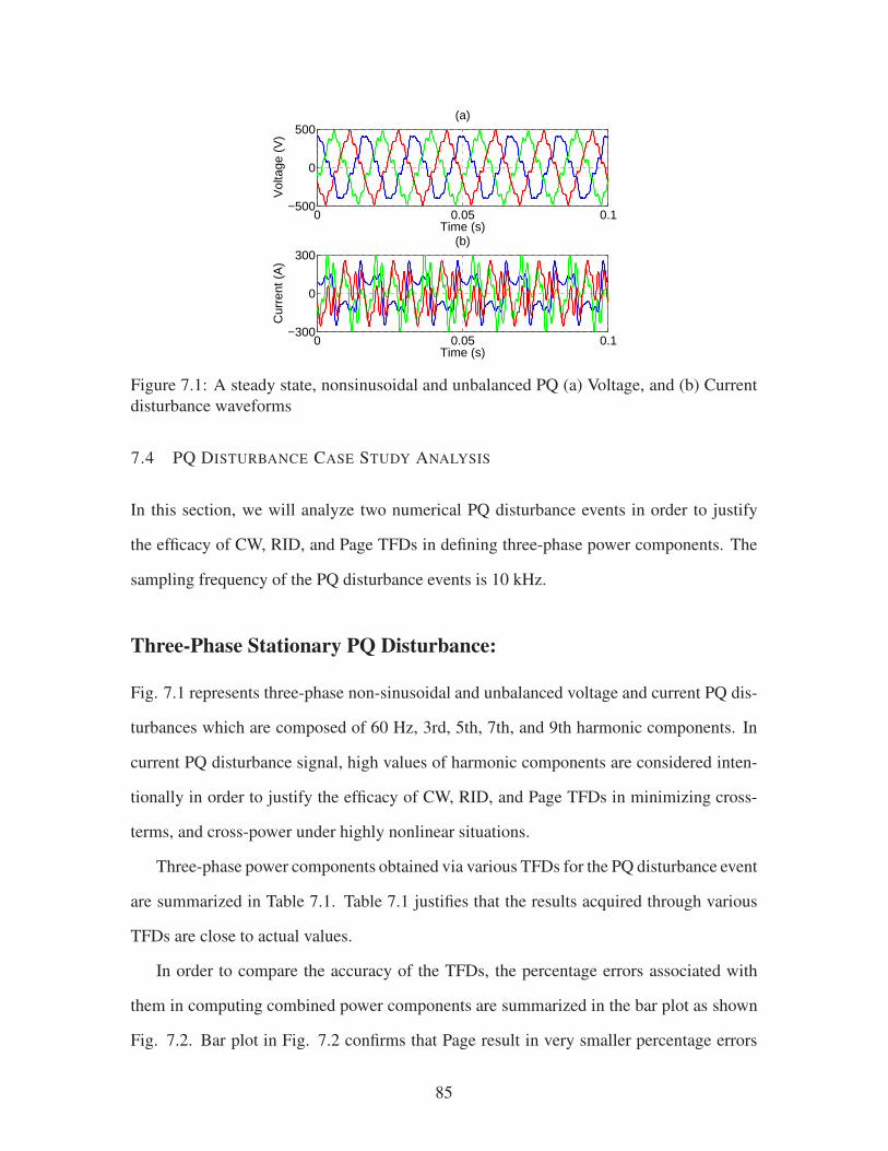
0 0.05 0.1−500
0
500
Time (s)
Vol
tage
(V
)
(a)
0 0.05 0.1−300
0
300
Time (s)
Cur
rent
(A
)
(b)
Figure 7.1: A steady state, nonsinusoidal and unbalanced PQ (a) Voltage, and (b) Current
disturbance waveforms
7.4 PQ DISTURBANCE CASE STUDY ANALYSIS
In this section, we will analyze two numerical PQ disturbance events in order to justify
the efficacy of CW, RID, and Page TFDs in defining three-phase power components. The
sampling frequency of the PQ disturbance events is 10 kHz.
Three-Phase Stationary PQ Disturbance:
Fig. 7.1 represents three-phase non-sinusoidal and unbalanced voltage and current PQ dis-
turbances which are composed of 60 Hz, 3rd, 5th, 7th, and 9th harmonic components. In
current PQ disturbance signal, high values of harmonic components are considered inten-
tionally in order to justify the efficacy of CW, RID, and Page TFDs in minimizing cross-
terms, and cross-power under highly nonlinear situations.
Three-phase power components obtained via various TFDs for the PQ disturbance event
are summarized in Table 7.1. Table 7.1 justifies that the results acquired through various
TFDs are close to actual values.
In order to compare the accuracy of the TFDs, the percentage errors associated with
them in computing combined power components are summarized in the bar plot as shown
Fig. 7.2. Bar plot in Fig. 7.2 confirms that Page result in very smaller percentage errors
85

Table 7.1: Three-Phase Power Components in pu Obtained via various TFDs for Stationary
PQ Disturbance case study (Sbase = 100 kVA, Vbase = 380 V)
Components Analysis Methods
Combined
Actual Value CW RID Page
Se = 4.2149 4.2168 4.2167 4.2139
P = 2.9062 2.8673 2.8673 2.8657
N = 3.0528 3.0919 3.0919 3.0894
PF = 0.6895 0.6800 0.6800 0.6801
Fund.
Se1 = 2.9375 2.9399 2.9398 2.9374
S+1 = 2.8866 2.8918 2.8917 2.8894
SU1 = 0.5447 0.5298 0.5298 0.5292
P+1 = 2.8611 2.8663 2.8662 2.8639
Q+1 = 0.3828 0.3831 0.3831 0.3828
PF+I = 0.9912 0.9912 0.9912 0.9912
LU = 0.1887 0.1832 0.1832 0.1831
Nonfund.
SeN = 3.0227 3.0230 3.0230 3.0213
SeH = 0.4701 0.4698 0.4698 0.4697
PH = 0.0413 0.0412 0.0412 0.0412
DeI = 2.9490 2.9493 2.9493 2.9476
DeV = 0.4682 0.4683 0.4683 0.4681
DeH = 0.4683 0.4680 0.4680 0.4679
HP = 1.0290 1.0283 1.0283 1.0285
Time tc (s) 268.353478 289.335297 35.3866
than the CW and RID TFDs. Also, computational time tc associated with Page TFD is
35.3866 s which is much smaller than the CW and RID TFDs.
86

Se P N PF0
0.7
1.4
%|E
rror
|
CWRIDPage
Figure 7.2: Percentage errors associated with various TFDs for three-phase stationary PQ
disturbance case study
0 0.05 0.1−200
0
200
Vol
tage
(V
)
Time (s)
(a)
0 0.05 0.1−50
0
50
Cur
rent
(A
)
Time (s)
(b)
Figure 7.3: Three-phase nonstationary PQ disturbance-(a) Voltage sag, and corresponding
(b) Current disturbance waveforms
Three-Phase Nonstationary PQ Disturbance:
In order to justify the efficacy of various TFDs under nonstationary PQ disturbance events,
three-phase voltage sag and corresponding current disturbances shown in Fig. 7.3 are con-
sidered. In this case study, the voltage and current signals are consist of 60 Hz, 3rd, 5th,
and 7th harmonic components.
The results of the voltage sag case study are summarized in Table 7.2. Table 7.2 shows
that all the TFDs provide very accurate results, however, Page TFD provides more accu-
rate results in the assessment of most of the power components. To illustrate further, the
percentage errors associate with various TFDs in computing combined power components
are shown in Fig. 7.4. Bar plot in Fig. 7.4 justifies that in computing combined power
components such as Se, P, and N the percentage errors associated with Page TFD are much
87

Table 7.2: Three-Phase Power Components in pu Obtained via various TFDs for nonsta-
tionary PQ disturbance case study (Sbase = 100 kVA, Vbase = 380 V)
Components Analysis Methods
Combined
Actual Value CW RID Page
Se = 4.8302 4.8270 4.8270 4.8294
P = 3.1043 3.0782 3.0783 3.0818
N = 3.7005 3.7181 3.7180 3.7182
PF = 0.6427 0.6377 0.6377 0.6381
Fund.
Se1 = 4.7563 4.7530 4.7531 4.7554
S+1 = 4.7129 4.7210 4.7210 4.7221
SU1 = 0.59289 0.55103 0.55146 0.56191
P+1 = 3.0558 3.0620 3.0629 3.0646
Q+1 = 3.5962 3.5934 3.5930 3.5926
PF+I = 0.6475 0.6486 0.6487 0.6490
LU = 0.1256 0.1185 0.1168 0.1190
Nonfund.
SeN = 0.84172 0.84161 0.84162 0.84189
SeH = 0.071508 0.071530 0.071532 0.071544
PH = 0.027490 0.027633 0.027634 0.027647
DeI = 0.51203 0.51186 0.51187 0.51205
DeV = 0.664424 0.664215 0.66425 0.66443
DeH = 0.066012 0.065977 0.065980 0.065987
HP = 0.1770 0.1771 0.1771 0.1770
Time tc (s) 257.2129 279.1455715 33.637336
smaller than the CW and RID TFDs. Also, computational speed in Page TFD is faster
than the CW and RID TFDs. Therefore, Page TFD can be employed in defining three-
phase power components under both steady state and nonstationary PQ disturbance events
which minimizes cross-terms, and cross-power efficiently, provides very accurate results
and faster computational speed.
88

Se P N PF0
0.5
1.0
%|E
rror
|
CWRIDPage
Figure 7.4: Percentage errors associated with various TFDs for three-phase voltage sag
case study
Utilizing the proposed method, one can also estimate the three-phase power compo-
nents for other types of nonstationary PQ disturbance events, such as voltage swell, tran-
sients, etc. However, the method will have the limitation as there is no TFD method that can
minimize the cross-terms in TFD, and cross-power in cross TFD completely. Therefore,
the efficacy of other bilinear TFD methods, such as Born-Jordan, Rihaczek, Zhao-Altas-
Mark, that can minimize the cross-terms [16] and cross-power as well, can be investigated
in computing three-phase components according to the IEEE Standard 1459-2010.
7.5 CONCLUSION
In this chapter, three-phase power components are redefined in the time-frequency domain
according to the IEEE Standard 1459-2010 based on the time marginal property of Page
TFD. Utilizing time-marginal property, Page TFD preserves simultaneous time and vari-
able frequency information, and provides very accurate assessment of three-phase power
components under PQ disturbance events. The efficacy of the proposed method has been
justified by employing it to stationary and nonstationary PQ disturbances.
Also, the accuracy of the proposed Page TFD based power components assessment
method has been compared to CW and RID TFDs for the PQ disturbances. The three-
phase power components for stationary and nonstationary PQ disturbances confirm that the
proposed Page TFD-based method provides more accurate results, and faster computational
speed than the CW and RID methods. Therefore, the proposed page TFD based method
89

can be a viable alternative for the assessment of three-phase power components according
to the IEEE Standard 1459-2010.
90
CHAPTER 8
A NEW PERSPECTIVE FOR WIND POWER GRID CODES
UNDER POWER QUALITY DISTURBANCES
8.1 INTRODUCTION
With increased penetration of wind energy, Federal Energy Regulatory Commission (FERC)
in the US sets forth requirements and grid codes specific to wind generating plants. The
grid codes issued by the FERC for a wind generating plant interconnection are summarized
into three main kinds as follows [77]:
1. Low Voltage Ride Through (LVRT) Capability: The first grid code focuses on
the low voltage ride through (LVRT) capability of a wind generating plant. As seen in
the LVRT curve provided in Fig. 8.1, the two key aspects of this regulation are - a wind
generating plant must have the LVRT capability down to 15 % of the rated line voltage
for 0.625 s, and must be able to operate continuously at 90 % of the rated line voltage,
measured at the high voltage side of the wind generating plant substation transformer(s).
2. Power Factor Design Criteria: According to the second grid code, the power factor
of a wind generating plan shall remain within the range of 0.95 leading to 0.95 lagging
measured at the point of common coupling (PCC) in order to ensure electric power system
reliability.
3. Supervisory Control and Data Acquisition Capability: To ensure system reli-
ability, the wind generating plant should have supervisory control and data acquisition
(SCADA) system to transmit data and receive instructions from the transmission provider.
The LVRT capability of a wind generating plant has been heavily studied in recent years
91

−1 0 0.625 1 2 3 40
0.15
0.6
0.91
1.2
Vol
tage
at t
he P
CC
(pu
)
Time (s)
must remain on−line
not required to remain on−line
Figure 8.1: Low voltage ride through curve by FERC.
[102]-[106]. In order to enhance the LVRT capability of a wind generating plant, the rms
voltage caused by a wind generating plant at the PCC should be assessed accurately. In-
accurate assessment of rms voltage may lead to unnecessary trip of the wind generating
plant from the grid. Also, to ensure electric power system reliability and fulfill the grid
codes, power factor and supervisory data acquisition of a wind generating plant should be
obtained precisely. FFT-based method is commonly used to assess rms voltage, power fac-
tor and provide useful information for SCADA system such as real power, reactive power,
apparent power, total harmonic distortion (THD) of a wind generating plant.
The FFT requires the signal to be periodic in nature, and only provides accurate assess-
ment in steady state [25]. However, a wind generating plant may introduce low voltage at
the PCC caused by uneven power production or a power system fault. Also, transient volt-
age disturbances are introduced by wind generating plants when they are connected to or
disconnected from the grid [80], [107]-[108] and by events as capacitors switching [109].
Furthermore, harmonics are injected into the grid by variable speed wind generating plants
due to the switching of power electronic converters. Therefore, from the electrical grid
perspective, wind generating plants are perceived as fluctuating power sources, and can be
best described as transient, nonsinusoidal and unbalance in nature [110]-[113]. Under such
conditions, the signal becomes aperiodic, and the frequency contents of the signal change
92

with time as well. Hence, the FFT-based method provides erroneous results in the presence
of wind generating plant disturbance events [25], and also it cannot provide any time in-
formation which may be a challenge for transmission providers to verify wind power grid
codes and protect power system reliability.
With regards to the aforementioned issues, time-frequency analysis (TFA) can play a
significant to conform wind power grid codes requirement since it has the ability to provide
simultaneous time and variable frequency information of wind generating plant disturbance
events. The application of the TFA in wind power has been demonstrated in several works
[23]-[24], [114]. However, assessments of rms voltage, power factor, and data acquisition
for supervisory control system under transient, nonsinusoidal and unbalanced conditions
have not been addressed in these works. Also, in [23]-[24], TFD-based THD is employed
for grid PQ analysis of wind power. The method defines the THD based on the energy
ratio of the fundamental and harmonic components instead of the rms values, nonetheless,
[23]-[24] provide inaccurate assessments of wind PQ.
In this chapter, a new method is proposed for the verification of wind power grid codes
based on TFA. Unlike the FFT, the method is able to assess the LVRT capability and power
factor of a wind generating plant, and acquire data for SCADA system accurately under
transient, nonsinusoidal, and unbalanced conditions. In addition, employing the proposed
method, the instantaneous direction of active and reactive power flow in a wind generating
can be determined by which transmission provider can take necessary steps to protect sys-
tem reliability in case of large amount of reverse active power flow from the grid to a wind
generating plant under PQ disturbance events. The effectiveness of the proposed method
will be justified by applying it to real-world wind generating plant disturbance events col-
lected from 150 MW Trent Mesa wind project in Texas.
93

8.2 POWER QUALITY INDICES FOR WIND POWER GRID CODES
In this section, we will utilize a set of PQ indices based on time-frequency analysis (TFA)
which will be used to verify the first two wind power grid codes, and data acquisition for
supervisory control system under transient, non-sinusoidal and unbalanced conditions.
1. TFA Based Effective RMS Voltage: The first grid code which provides information
about LVRT capability can be verified by defining the effective rms voltage Ve under tran-
sient, nonsinusoidal and unbalanced conditions according to the IEEE Standard 1459-2010
[13] as follows:
Ve =
√
(V T FAa )
2+(V T FA
b )2+(V T FA
c )2
3(8.1)
where V T FAa ,V T FA
b and V T FAc are TFA based effective rms voltage of phase A, phase B, and
Phase C of wind generating plant disturbance events, respectively.
2. TFA Based Effective Power Factor: The second grid code emphasizes on wind
generating plant power factor requirement and can be verified by defining the effective
power factor PFe under transient, nonsinusoidal and unbalanced conditions based on the
TFA method as follows:
PFe =P
Se=
P
3 ·Ve · Ie(8.2)
where
Ie =
√
(ITFAa )
2+(ITFA
b )2+(ITFA
c )2
3(8.3)
P = PT FAa +PT FA
b +PT FAc (8.4)
where Ie and P are the effective rms current and total active power of the wind generating
plant, respectively.
3. TFA Based Data Acquisition for SCADA System: SCADA system of a wind
generating plant is used to provide long-term databases on the farm level so that service
engineers can use a central application in the control desk to access and monitor the com-
plete range of up-to-the-minute data from all connected wind turbine generator units to
94

carry out any kind of comparative analysis. For the instantaneous analysis and monitoring
purpose of a wind generating plant data, in this chapter we will obtain voltage and current
THDs, active power, apparent power, reactive power and harmonic pollution information
for the SCADA system employing the TFA method.
Equivalent Total Harmonic Distortion
THD is the commonly used power quality factor to quantify harmonics injection into grid
by a variable speed wind generating plant. The equivalent voltage T HDeV and current
T HDeI for a variable speed wind generating plant can be assessed as:
T HDeV =V T FA
eH
V T FAe1
(8.5)
T HDeI =IT FAeH
IT FAe1
(8.6)
where Ve1, VeH and Ie1, IeH are TFA based effective fundamental and harmonics rms voltage
and current, respectively. Harmonics and fundamental frequency components are separated
employing the method in [25].
Active Power
The positive sequence active power P+1 , harmonic active power PH , and the total active
power P of a wind generating plant are obtained as:
P+1 =
1
2T
t∫
t−T
ℜ
{∫
ω
CT FDv+1 i+1(t,ω;φ)dω
}
dt (8.7)
PH =1
2T
t∫
t−T
ℜ
{∫
ω
CT FDvH iH (t,ω;φ)dω
}
dt (8.8)
P = Pa +Pb +Pc (8.9)
where CT FDv+1 i+1(t,ω;φ) and CT FDvH iH (t,ω;φ) are the cross time-frequency distributions
of the positive sequence and harmonic voltage and current, respectively, and Pa, Pb, and Pc
95

are three-phase power obtained via cross time-frequency distributions of respective voltage
and current, respectively.
Apparent Power
The TFA based effective harmonic apparent power SeH , non-fundamental apparent power
SeN and total apparent power Se [13] for a wind generating plant are defined as:
SeH = ST FAe1 ·THDeV ·THDeI (8.10)
SeN = ST FAe1 ·
√
T HDeV +T HDeI +T HDeV ·T HDeI (8.11)
Se =√
S2e1 +S2
eN (8.12)
Reactive Power
The most suggested reactive power expression is the fundamental positive sequence reac-
tive power [13] which is defined as:
Q+1 = 3 · 1
2· 1
T
t∫
t−T
ℑ
{∫
ω
CT FDv+i+(t,ω;φ)dω
}
dt (8.13)
Harmonic Pollution
The harmonic pollution injected by a variable speed wind generating plant into the grid can
be obtained for SCADA system as:
HP =SeN
Se1(8.14)
The TFA based method discussed in this section will be employed to computer sim-
ulated and real-world power quality disturbance events for wind power grid codes under
transient, nonsinusoidal, and unbalanced conditions in the next section.
96

Ve PF THDeVTHDeI P1+ PH P SeH SeN Se Q1+ HP
0.25
0.50
0.75
1.0
%|E
rror
|
Figure 8.2: Percentage errors associated with the simulated state case study analysis.
8.3 SIMULATED CASE STUDY
In order to justify the efficacy of the proposed method, the following computer simulated
three-phase nonsinusoidal and unbalanced voltage signals are considered:
va(t) = 1√
2cos(ω1t −0.740) (8.15)
+0.2√
2cos(ω3t +6.760)+0.1√
2cos(ω5t +142.30)
vb(t) = 1.1√
2cos(ω1t −121.20) (8.16)
+0.15√
2cos(ω3t +6.280)+0.05√
2cos(ω5t +167.40)
vc(t) = 1.05√
2cos(ω1t +121.30) (8.17)
+0.1√
2cos(ω3t +9.70)+0.15√
2cos(ω5t +157.70)
The respective three-phase currents signals are as follows:
ia(t) = 1√
2cos(ω1t −220) (8.18)
+0.25√
2cos(ω3t +1200)+0.2√
2cos(ω5t −1750)
ib(t) = 0.95√
2cos(ω1t −120.80) (8.19)
+0.15√
2cos(ω3t +99.490)+0.1√
2cos(ω5t +65.090)
ic(t) = 0.9√
2cos(ω1t +120.30) (8.20)
+0.01√
2cos(ω3t +100.010)+0.05√
2cos(ω5t +57.70)
As seen in the Eqs. (8.15)-(8.20), the voltage and currents signals are unbalanced and com-
posed of fundamental, 3rd and 5th harmonic components. The percentage errors associated
97

CIRCUIT #2
CIRCUIT #1
CIRCUIT #3
CIRCUIT #4
CIRCUIT #5
138 kV BUS
34.5 kV BUS
34.5 kV CIRCUIT
BREAKERS
PCC
34.5 kV:138 kV
Win
dD
FIG
Y
Win
dD
FIG
Y
Win
dD
FIG
Y
Win
dD
FIG
Y
Win
dD
FIG
Y
Win
dD
FIG
Y
Win
dD
FIG
Y
16
*1
.5=
24
MW
17
*1
.5=
25
.5 M
W
33
*1
.5=
49
.5 M
W
3*
1.5
=4
.5 M
W
11
*1
.5=
16
.5 M
W
4*
1.5
=6
MW
16
*1
.5=
24
MW
Figure 8.3: Simplified one-line diagram of Trent Mesa wind project.
with the Page TFD-based method for the simulated case study are summarized in Fig. 8.2.
We utilize the Page TFD as it provides more accurate results, and faster computational
speed than the RID and CW TFDs as discussed in the previous chapter. Fig. 8.2 shows that
Page TFD-based method results in very small percentage errors (less than 1%), therefore,
the proposed method can be employed for wind power grid codes which we will discuss in
the next section.
8.4 STUDIED WIND GENERATING PLANT
The Real-world wind generating plant PQ disturbance events were recorded from Trent
Mesa wind project in Texas, and provided by the courtesy of National Renewable Energy
Laboratory (NREL). The one-line diagram of the Trent Mesa wind generating plant is pro-
vided in Fig. 8.3. The wind generating plant consists of 100 General Electric (GE) 1.5
MW wind turbine generators for a total capacity of 150 MW. The disturbance events are
measured from the high voltage side of the substation transformer at the point of common
98

0.03 0.10 0.16−100
0
100
Vol
tage
(kV
)
(a)
Time (s)
0.03 0.10 0.16
−1
0
1
Cur
rent
(kA
)
(b)
Time (s)
Figure 8.4: (a) Voltage sag, and (b) Current disturbance waveforms.
coupling (PCC) as seen in the figure, and the sampling frequency of the disturbance wave-
forms is 7678.99 Hz. We will analyze three different disturbance events to demonstrate the
efficacy of the proposed TFA based method for wind power grid codes - a voltage sag, a
transient and an oscillatory type disturbances.
Voltage Sag Case Study
Figs. 8.4 (a) and (b) show voltage sag, and corresponding current disturbance waveforms,
respectively. The following observations are summarized based on the TFA based analysis
of the voltage sag case study provided in Fig. 8.5.
Fig. 8.5(a1) shows the effective rms voltage at the PCC stays above 0.9 pu both in
steady state and sag conditions, and meets the first grid code requirement by the FERC.
As seen in Fig. 8.5(a2), the power factor is lagging in steady state and leading during
the voltage sag. In both conditions, power factor of the wind generating plant is below 0.95
leading to 0.95 lagging, and does not conform the second grid code requirement issued by
the FERC.
Figs. 8.5(a3) and (a4) illustrate that voltage THD increases and current THD decreases
during the voltage sag because of the decrease in the fundamental voltage and increase in
99

0.03 0.10 0.16
−0.95
0
0.95
PF
e (pu
)
(a2)
0.03 0.10 0.160.8
0.9
1.0V
e (pu
)
(a1)
0.03 0.10 0.162.5
7.5
12
TH
DeV
(%
)
(a3)
0.03 0.10 0.16
16
45
90
TH
DeI
(%
)
(a4)
0.03 0.10 0.16−5
−2
01
x 107
P1+ (
W)
(b1)
0.03 0.10 0.160
7
14x 10
7
Time (s)
Se (
VA
)
(c2)
0.03 0.10 0.160.1
1.5
3x 10
6
SeH
(V
A)
(b4)
0.03 0.10 0.16
0.28
1.5
3x 10
7
Time (s)
SeN
(V
A)
(c1)
0.03 0.10 0.16−10
−5
0
5x 10
5
PH
(W
)
(b2)
0.03 0.10 0.16−4
−2
00.5
x 107
P (
W)
(b3)
0.03 0.10 0.16−9
−4
01
x 107
Time (s)Q
1+ (
VA
r)
(c3)
0.03 0.10 0.160.12
0.75
1.5
Time (s)
HP
(pu
)
(c4)
Figure 8.5: Results of voltage sag case study analysis - Effective (a1) rms voltage, (a2)power Factor, (a3) Voltage THD, (a4) Current THD, (b1) Positive sequence active power,
(b2) Harmonic active power, (b3) Total active power, (b4) Harmonic apparent power, (c1)Non-fundametnal apparent power, (c2) Total apparent power, (c3) Positive sequence reac-
tive power, and (c4) Harmonic pollution factor.
the fundamental current, respectively. In addition, the voltage THD is above 2.5% limit
recommended by the IEEE Standard 519 [10] for 138 kV system.
The positive sequence active power P+1 , harmonic active power PH , and total active
power P flow from the grid to the wind farm during voltage sag as observed in Figs.
8.5(b1)-(b3), respectively. Also, in the steady state the wind generating plant delivers
approximately 5 MW power only whereas 40 MW power flows from grid to the wind
farm during the voltage sag. This reverse power flow may increase the rotor speed, and
result in mechanical damage of wind generating units in the plant. Under such condition,
disconnection of a wind generating plant may be required by the transmission provider in
order to protect system reliability even though the wind generating plant satisfies the LVRT
capability shown in Fig. 8.5(a1).
100

0.02 0.04 0.06−100
0
100
Vol
tage
(kV
)
Time (s)
(a)
0.02 0.04 0.06
−0.5
0
0.5C
urre
nt (
kA)
Time (s)
(b)
Figure 8.6: Transient (a) Voltage, and (b) Current disturbance waveforms.
The effective harmonic apparent power SeH , non-fundamental apparent power SeN and
total apparent Se of the wind generating plant are summarized in Figs. 8.5(b4), (c1) and
(c2), respectively. The total apparent power of the wind generating plant is increased to
approximately 140 MVA by the voltage sag disturbance as seen in Fig. 8.5(c2).
The positive sequence reactive power of the wind generating plant is positive in the
steady state, however, is negative and flows from grid to the wind generating plant during
the sag as seen in Fig. 8.5(c3).
Fig. 8.5(c4) shows that harmonic pollution injected by the Trent Mesa wind generating
plant into 138 kV grid is above 0.12 pu.
Transient Case Study
The transient voltage and current disturbances for the study of wind power grid codes are
incorporated in Figs. 8.6 (a) and (b), respectively. The results of the transient disturbance
case study are provided in Fig. 8.7, and summarized in the following contexts.
Fig. 8.7(a1) shows that transient disturbance causes overvoltage at the PCC, however,
the effective rms voltage Ve is above 0.9 pu both in normal and transient operating condi-
tions, and meets the first grid code requirement.
101

0.02 0.04 0.060.95
1.0
1.05V
e (pu
)
(a1)
0.02 0.04 0.060.95
0.975
1.0
PF
e (pu
)
(a2)
0.02 0.04 0.060.57
5
10
TH
DeV
(%
)
(a3)
0.02 0.04 0.06
0.86
2
4
TH
DeI
(%
)
(a4)
0.02 0.04 0.060.8
1.1
1.4x 10
8
P1+ (
W)
(b1)
0.02 0.04 0.060
2
4x 10
5
SeH
(V
A)
(b4)
0.02 0.04 0.060
7.5
15x 10
6
SeN
(V
A)
(c1)
0.02 0.04 0.06−10
0
5x 10
4
PH
(W
)
(b2)
0.02 0.04 0.061.08
1.123
1.16x 10
8
P (
W)
(b3)
0.02 0.04 0.061.127
1.131
1.135x 10
8
Time (s)
Se (
VA
)
(c2)
0.02 0.04 0.06−1.3
−1.1
−0.9x 10
7
Time (s)
Q1+ (
VA
r)
(c3)
0.02 0.04 0.060.01
0.05
0.1
Time (s)
HP
(pu
)
(c4)
Figure 8.7: Results of trasient case study analysis - Effective (a1) rms voltage, (a2) power
Factor, (a3) Voltage THD, (a4) Current THD, (b1) Positive sequence active power, (b2)Harmonic active power, (b3) Total active power, (b4) Harmonic apparent power, (c1) Non-
fundametnal apparent power, (c2) Total apparent power, (c3) Positive sequence reactive
power, and (c4) Harmonic pollution factor.
The effective power factor PFe in Fig. 8.7(a2) is lagging and above 0.95 pu, hence,
reliability of the wind farm is not compromised by the transient disturbance according to
the second grid code.
Fig. 8.7(a3) and (a4) show that the voltage THD at the PCC is below 2.5% in steady
state, however, transient disturbance causes the voltage and current THDs increase to ap-
proximately 10% and 4%, respectively because of the presence of high harmonic compo-
nents in the transient voltage and current disturbances.
Unlike the voltage sag, in case of the transient case study, both the positive sequence
active power P+1 and total active power P flow from wind farm to the grid, only the har-
monic active power PH flows in the opposite direction as observed in Fig. 8.7(b1)-(b3).
Also, the wind generating plant delivers almost 112.3 MW power into the grid out of rated
102

0.02 0.035 0.05−100
0
100
Vol
tage
(kV
)
Time (s)
(a)
0.02 0.035 0.05
−0.1
0
0.1C
urre
nt (
kA)
Time (s)
(b)
Figure 8.8: Oscillatory (a) Voltage, and (b) Current disturbance waveforms.
150 MW power.
Figs. 8.7(b4)-(c2) illustrates that the apparent power of the wind generating plant are
increased by the transient disturbance. The positive sequence reactive power of the wind
generating plant is negative and flows from grid to the wind generating plant as seen in Fig.
8.7(c3). Fig. 8.7(c4) shows that the transient disturbance increases the harmonic pollution
injection into the grid to 0.1 pu approximately.
Oscillatory Case Study
A wind generating plant typically consists of vast underground cables, reactive compensa-
tion equipment, transformers, wind turbine generators with internal power factor correction
capacitors. The energy exchange between inductive and capacitive elements of a wind gen-
erating plant may lead to harmonic resonance and introduce oscillatory type disturbance
into the grid. Figs. 8.8(a)-(b) represent oscillatory type voltage and current disturbance
waveforms recorded from the Trent Mesa wind project. The corresponding TFA based
analysis results are summarized in Fig. 8.9, and the following perceptions are made based
on the case study analysis.
In the oscillatory case study, the effective rms voltage in Fig. 8.9(a1) is above 0.9
103

0.02 0.035 0.050.95
1.0
1.05V
e (pu
)
(a1)
0.02 0.035 0.05−0.95
0
0.95
PF
e (pu
)
(a2)
0.02 0.035 0.050.8
5
10
TH
DeV
(%
)
(a3)
0.02 0.035 0.059
150
300
TH
DeI
(%
)
(a4)
0.02 0.035 0.05−3.5
−3
−2.5x 10
5
P1+ (
W)
(b1)
0.02 0.035 0.050
3.5
7x 10
5
SeH
(V
A)
(b4)
0.02 0.035 0.050
5
10x 10
6
Time (s)
SeN
(V
A)
(c1)
0.02 0.035 0.05−15
−7.5
0x 10
4
PH
(W
)
(b2)
0.02 0.035 0.05−4.5
−3.5
−2.5x 10
5
P (
W)
(b3)
0.02 0.035 0.052
7
12x 10
6
Time (s)
Se (
VA
)
(c2)
0.02 0.035 0.053.42
3.45
3.48x 10
6
Time (s)Q
1+ (
VA
r)
(c3)
0.02 0.035 0.050.09
1.5
3
Time (s)
HP
(pu
)
(c4)
Figure 8.9: Results of oscillatory case study analysis - Effective (a1) rms voltage, (a2)power Factor, (a3) Voltage THD, (a4) Current THD, (b1) Positive sequence active power,
(b2) Harmonic active power, (b3) Total active power, (b4) Harmonic apparent power, (c1)Non-fundametnal apparent power, (c2) Total apparent power, (c3) Positive sequence reac-
tive power, and (c4) Harmonic pollution factor.
pu, and the wind generating plant fulfills the first grid code requirement, however, the
effective power factor is leading and close to zero, and fails to meet the required power
factor criteria according to the second grid code as observed in Fig. 8.9(a2). Also, in Figs.
8.9(a3)-(a4), the effective voltage THD is low compared to very high value of current THD
(approximately 300%) during the oscillation. This is an indication of series resonance,
where very high value of harmonic current is observed, in the wind generating plant.
All the positive sequence active power P+1 , harmonic active power PH and total active
power P flow from the grid to the wind generating plant as seen in Figs. 8.9(b1)-(b3),
respectively. The apparent power information for the SCADA system are incorporated
in Figs. 8.9(b4)-(c2). As we can see in Figs. 8.9(b4)-(c1), the oscillatory disturbance
increases the harmonic and non-fundamental apparent power from 0 to 0.7 MVA and 10
104

Table 8.1: Summary of Case Study Analysis Results
Case Study Analysis
SCADA DATA Indices Volt. sag Tran. Osc.
RMS Volt. (pu) Ve 0.9556 1.002 1.0002
Power Factor (pu) PFe 0.1136 0.9937 -0.0576
THD%T HEeV 6.990 4.567 4.234
T HDeI 35.18 2.010 174.7
Active Power (MW)
P+1 -12.96 112.23 -0.3203
PH -0.1590 -0.0319 -0.0622
P -12.34 112.27 -0.3816
Apparent Power (MVA)
SeH 0.9755 0.1469 0.3353
SeN 13.51 5.731 6.136
Se 62.79 112.98 7.462
Reactive Power (MVAr) Q+1 -33.34 -10.61 3.456
Harmonic Pollution (pu) HP 0.3634 0.0508 1.751
Grid CodesIst yes yes yes
2nd no yes no
MVA, respectively.
Fig. 8.9(c3) represents the positive sequence reactive power is constant, and flows
from the wind generating plant to the grid. Also, the oscillatory disturbance causes the
harmonic pollution to increase to a relatively high value of 3 pu approximately compared
to the previous two case studies.
The TFA based method provides instantaneous assessment of the effective rms voltage,
power factor and supervisory data for a wind generating plant. However, in order to provide
more informative and convenient comparison of the three case studies analysis, TFA based
PQ (TFAPQ) indices for wind power grid codes are quantified as a single value which is
defined as follows:
105

T FAPQ =1
T
∫ T
0T FAPQ(t)dt (8.21)
The results of the three wind generating plant PQ disturbance events are provided in Ta-
ble 8.1. As seen in the table, the effective rms voltage is above 0.9 pu in all three PQ
disturbances, therefore, the wind generating plant meets the first grid code requirement.
However, the plant maintains the required power factor criteria in case of the transient dis-
turbance only which is 0.9937 pu lagging. Also, in the transient disturbance, voltage and
current THDs are lower at the PCC, the wind generating plant delivers more power, and
harmonic pollution injected by the wind generating plant into the grid is much lower than
the voltage sag and oscillatory disturbances. Therefore, from PQ point of view, the wind
generating plant will have less impact on the electrical grid for the transient disturbance.
8.5 CONCLUSION
In this chapter, a new time-frequency analysis method is proposed for wind power grid
codes under transient, nonsinusoidal and unbalanced PQ disturbance events. The effi-
cacy of the proposed method has been justified by employing it to a computer simulated
and real-world wind generating plant PQ disturbances. Unlike the traditional FFT-based
method, the proposed technique extracts time information, and provides instantaneous and
accurate assessment of effective rms voltage, power factor to verify wind power grid codes
under transient, nonsinusoidal, and unbalanced conditions. Also, employing the proposed
method, dynamic signature of the wind generating plant PQ disturbance events can be ex-
tracted for SCADA system to protect system reliability. For example, in the voltage sag
case study, where large amount of reverse active power flows into the plant, disconnec-
tion of the wind generating plant may be required to ensure system reliability. In addition,
based on the SCADA information provided in this chapter, one can develop a supervisory
control system for a wind generating plant to fulfill the grid codes requirements which will
be discussed in the scope of future work.
106

CHAPTER 9
CONCLUSION
This dissertation has the following novel and significant contributions in the area of power
quality (PQ) and time-frequency distribution (TFD) which are summarized as follows:
• Although, TFDs have been frequently utilized for the detection, classification, and
assessment of PQ disturbances, there is no work devoted to defining rms value, aver-
age active power, and reactive power correctly employing TFDs. In this dissertation,
rms value, active power and reactive power are defined in the time-frequency domain
correctly by introducing the scale factors which will play a significant role for correct
assessment of PQ disturbances.
• Also, the existing transient PQ indices are redefined correctly for PQ disturbances
which provide much more accurate results than the FFT-based method for nonsta-
tionary PQ disturbances.
• Another novel contribution of this dissertation is redefining the single-phase and
three-phase power components according to the IEEE Standard 1459-2010 under
transient, sinusoidal, nonsinusoidal, balanced, or unbalanced conditions employing
TFD method. Utilizing the proposed method, one can find the direction of harmonic
active power flow to the network or to the load with time. Also, harmonic active
power is assessed directly utilizing time marginal property of the XTFD which pro-
vides very precise result.
• Utilizing the concept of TFD-based redefined three-phase power components, a new
perspective for wind power grid codes is proposed that is able to accomplish in-
107

stantaneous verification of wind power grid codes, issued by the FERC, under PQ
disturbances.
The TFD-based PQ analysis method provided in this dissertation can play a significant
role in the following future works:
• The redefined PQ indices provided in this dissertation can be employed to detect
and classify PQ disturbances as the PQ indices extract dynamic signature of PQ
disturbances.
• In this dissertation, the existing PQ index instantaneous frequency is utilized to es-
timate the fundamental frequency deviation of fixed speed wind energy conversion
systems. The instantaneous frequency can also be employed to variable speed wind
energy conversion systems to assess fundamental frequency deviation once funda-
mental frequency component is separated from the harmonic components.
• In [75], WV TFD method is employed for direction finding of capacitor switching
in electric power systems which may lead to erroneous results due to the presence
of cross-power as discussed in this dissertation. For more accurate assessment, RID,
CW, and Page TFDs can be employed for direction finding of capacitor switching.
• In this dissertation, frequency components responsible for transient disturbances are
identified. Therefore, the impact of transient disturbances on electric power systems
can be minimized by designing and employing appropriate filter to remove the tran-
sient frequency components.
• Also, time-varying active power and reactive power information are provided uti-
lizing the XTFD which can be employed to design super capacitor energy storage
system, and reactive power compensator, respectively to enhance the PQ in electric
power systems.
108

BIBLIOGRAPHY
[1] S. M. Peeran, and C. W. P. Cascadden, “Application, Design, and Specification of
Harmonic Filters for Variable Frequency Drives,” IEEE Transactions on Industry Ap-
plications, vol. 31, no. 4, pp.841-847, July/August 1995.
[2] P. W. Hammond, “A New Approach to Enhance Power Quality for Medium Voltage
AC Drives,” IEEE Transactions on Industry Applications, vol. 33, no. 1, pp. 202-208,
January/February 1997.
[3] Y. Liu, G. T. Heydt, and R. F. Chu, “The Power Quality Impact of Cycloconverter
Control Strategies,” IEEE Transactions on Power Delivery, vol. 20, no. 2, pp. 1711-
1718, April 2005.
[4] J. Mazumdar, R. G. Harley, and F. C. Lambert, and G. K. Venayagamoorthy, “Neural
Network Based Method for Predicting Nonlinear Load Harmonics,” IEEE Transac-
tions on Power Electronics, vol. 22, no. 3, pp.1036-1045, May 2007.
[5] B. M. Dehkordi, M. Moallem, and A. Parsapour, “Predicting Foaming Slag Quality in
Electric Arc Furnace Using Power Quality Indices and Fuzzy Method,” IEEE Transac-
tions on Instrumentation and Measurement, vol. 60, no. 12, pp. 3845-3852, December
2011.
[6] S. K. Jain, S. N. Singh, and J. G. Singh, “An Adaptive Time-Efficient Technique
for Harmonic Estimation of Nonstationary Signals,” IEEE Transactions on Industrial
Electronics, vol. 60, no. 8, pp. 3295-3303, May 2012.
[7] D. Somayajula, and M. L. Crow, “An Ultracapacitor Integrated Power Conditioner for
Intermittency Smoothing and Improving Power Quality of Distribution Grid,” IEEE
Transactions on Sustainable Energy, vol. 5, no. 4, pp. 1145-1155, October 2014.
[8] K. Koziy, B. Gou, and J. Aslakson, “A Low-Cost Power-Quality Meter With Series
Arc-Fault Detection Capability for Smart Grid,” IEEE Transactions on Power Delivery,
vol. 28, no. 3, pp. 1584-1591, July 2013.
[9] G. T. Heydt, and W. T. Jewell, “Pitfalls of Electric Power Quality Indices,” IEEE Trans-
actions on Power Delivery, vol. 13, no. 2, pp. 570-578, April 1998.
109

[10] IEEE Recommended Practice for power and Grounding Electronic Equipment, 1999.
IEEE Std. 1100-1999, IEEE Press.
[11] IEC61400-21, Measurement and Assessment of Power Quality Characteristics of
Grid-Connected Wind Turbines, Ed. 1, 2008.
[12] IEEE Trial-Use Standard Definitions for the Measurement of Electric Power Quan-
tities Under Sinusoidal, Non-sinusoidal, Balanced, Or Unbalanced Conditions, IEEE
Standard 1459-2000, 2000.
[13] IEEE Standard Definitions for the Measurement of Electric Power Quantities Un-
der Sinusoidal, Non-sinusoidal, Balanced or Unbalanced Conditions, IEEE Standard
1459-2010, March 2010.
[14] C. Gherasim, J. V. den Keybus, J. Driesen, and R. Belmans, “DSP Implementatin of
Power Measurements According to the IEEE Trial-Use Standard 1459,” IEEE Trans-
actions on Instrumentation and Measurement, vol. 53, no. 4, pp. 1086-1092, August
2004.
[15] A. Mansour, Z. Chengning, and H. Nasry, “Measurement of Power Components in
Balanced and Unbalanced Three-Phase Systems Under Nonsinusoidal Operating Con-
ditions by Using IEEE Standard 1459D1d’72010 and Fourier Analysis,” 2013 Interna-
tional Conference on Technological Advances in Electrical, Electronics and Computer
Engineering (TAEECE), pp. 166-171, 9-11 May 2013.
[16] L. Cohen, Time-Frequency Signal Analysis, Prentice Hall, New York, 1995.
[17] W. G. Morsi, and M. E. El-Hawary, “Reformulating Power Components Definitions
Contained in the IEEE Standard 1459-2000 Using Discrete Wavelet Transform,” IEEE
Transactions on Power Delivery, vol. 22, no. 3, pp. 1910-1916, July 2007.
[18] W. G. Morsi and M. E. El-Hawary, “Reformulating Three-Phase Power Components
Definitions Contained in the IEEE Standard 1459-2000 Using Discrete Wavelet Trans-
form,” IEEE Transactions on Power Delivery, vol. 22, no. 3, pp. 1917-1925, July
2007.
[19] W. G. Morsi, and M. E. El-Hawary, “A New Perspective for the IEEE Standard 1459-
2000 Via Stationary Wavelet Transform in the Presence of Nonstationary Power Qual-
ity Disturbance,” IEEE Transactions on Power Delivery, vol. 23, no. 4, pp. 2356-2365,
October 2008.
110

[20] W. G. Morsi, and M. E. El-Hawary, “Wavelet Packet Transform-Based Power Qual-
ity Indices for Balanced and Unbalanced Three Phase Systems Under Stationary and
Nonstationary Operating Conditions,” IEEE Transactions on Power Systems, vol. 24,
no. 4, pp. 2300-2310, October 2009.
[21] W. G. Morsi, C. P. Diduch, L. Chang, Koziy, and M. E. El-Hawary, “Wavelet Based
Reactive Power and Energy Management in the Presence of Power Quality Distur-
bances”, IEEE Transactions on Power Systems, vol. 26, no. 3, pp. 1263-1271, August
2011.
[22] Y. J. Shin, E. J. Powers, W. M. Grady, and A. Arapostathis, “Power Quality Indices
for Transient Disturbances,” IEEE Transactions on Power Delivery, vol. 21, no. 1, pp.
253-261, January 2006.
[23] P. Stone, M. Islam, and Y. J. Shin, “Power Quality Impact of Wind Turbine Generators
on the Electrical Grid,” Energy Tech, 2012 IEEE, Cleaveland, Ohio, USA, pp. 1-6, May
2012.
[24] M. Islam, H. A. Mohammadpour, P. Stone, and Y. J. Shin, “Time-frequency Based
Power Quality Analysis of Variable Speed Wind Turbine Generators,” Industrial Elec-
tronics Society, IECON 2013 - 39th Annual Conference of the IEEE, vol., no., pp.
6426-6431, 10-13 November 2013.
[25] M. Islam, H. A. Mohammadpour, A. Ghaderi, C. Brice, and Y. J. Shin, “Time-
frequency-Based Instantaneous Power Components for Transient Disturbances Ac-
cording to IEEE Standard 1459,” IEEE Transactions on Power Delivery, vol., no. 99,
pp., October 2014.
[26] H. Kim, F. Blaabjerg, and B. Bak-Jensen, “Spectral Analysis of Instantaneous Powers
in Single-Phase and Three-Phase Systems with Use of p-q-r Theory,” IEEE Transac-
tions on Power Electronics, vol. 17, no. 5, pp. 711-720, September 2002.
[27] J. I. Leon, R. Portillo, S. Vazquez, J. J. Padilla, L. G. Franquelo, and J. M. Carrasco,
“Simple Unified Approach to Develop a Time-Domain Modulation Strategy for Single-
Phase Multilevel Converters,” IEEE Transactions on Industrial Electronics, vol. 55, no.
9, pp. 3239-3248, September 2008.
[28] W. A. Omran, H. S. K. El-Goharey, M. Kazerani, and M. M. A. Salama, “Identifi-
cation and Measurement of Harmonic Pollution for Radial and Nonradial Systems,”
IEEE Transactions on Power Delivery, vol. 24, no. 3, pp. 1642-1650, July 2009.
111

[29] A. E. Emanuel, and D. L. Milanez, “Clarke’s Alpha, Beta, and Zero Components:
A Possible Approach for the Conceptual Design of Instrumentation Compatible with
IEEE Std. 1459-2000,” IEEE Transactions on Instrumentation and Measurement, vol.
55, no. 6, pp. 2088-2095, December 2006.
[30] A. Cataliotti, and V. Cosentino, “A Time-Domain Strategy for the Measurement of
IEEE standard 1459-2000 Power Quantities in Nonsinusoidal Three-Phase and Single-
Phase Systems,” IEEE Transactions on Power Delivery, vol. 23, no. 4, pp. 2113-2123,
October 2008.
[31] A. Cataliotti, V. Cosentino, and S. Nuccio, “A Virtual Instrument for the Measurement
of IEEE Std. 1459-2000 Power Quantities,” IEEE Transactions on Instrumentation and
Measurement, vol. 57, no. 1, pp. 85-94, Janruary 2008.
[32] A. Pigazo, and V. M. Moreno, “Accurate and Computationally efficient Implemen-
tation of the IEEE 1459-2000 Standard in Three-Phase Three-Wire Power Systems,”
IEEE Transactions on Power Delivery, vol. 22, no. 2, pp. 752-757, April 2007.
[33] J. J. Tomic, and M. D. Kusljevic, “An Adaptive Resonator-Based Method for Power
Measurements According to the IEEE Trial-Use Standard 1459-2000,” IEEE Trans-
actions on Intrumentation and Measurement, vol. 59, no. 2, pp. 250-258, February
2010.
[34] L. Angrisani, P. Daponte, M. D’Apuzzo, and A. Testa, “A Measurement Method
Based on the Wavelet Transform for Power Quality Analysis,” IEEE Transactions on
Power Delivery, vol.13, no.4, pp.990-998, October 1998.
[35] G. Zwe-Lee, “Wavelet-Based Neural Network for Power Disturbance Recogni-
tion and Classification,” IEEE Transactions on Power Delivery, vol. 19, no. 4, pp.
1560D1d’71568, October 2004.
[36] J. G. M. S. Decanini, M. S. Tonelli-Neto, F. C. V. Malange, and C. R. Minussi, “De-
tection and Classification of Voltage Disturbances Using a Fuzzy-ARTMAP-Wavelet
Network,” Electric Power System Research, vol. 81, no. 12, pp. 2057D1d’72065, De-
cember 2011.
[37] C. H. Lin, and C. H. Wang, “Adaptive Wavelet Networks for Power-Quality Detection
and Discrimination in a Power System,” IEEE Transactions on Power Delivery, vol.
21, no. 3, pp. 1106-1113, July 2006.
[38] S. J. Huang, T. M. Yang, and J. T. Huang, “FPGA Realization of Wavelet Transform
112

for Detection of Electric Power System Disturbances,” IEEE Transactions on Power
Delivery, vol. 17, no. 2, pp. 388-394, April 2002.
[39] U. D. Dwivedi, and S. N. Singh, “Enhanced Detection of Power-Quality Events Us-
ing Intra and Interscale Dependencies of Wavelet Coefficients,” IEEE Transaction on
Power Delivery, vol.25, no. 1, pp. 358-366, January 2010.
[40] A. Andreotti, A. Bracale, P. Caramia, and G. Carpinelli, “Adaptive Prony Method for
the Calculation of Power-Quality Indices in the Presence of Nonstationary Disturbance
Waveforms,” IEEE Transactions on Power Delivery, vol. 24, no. 2, pp. 874-883, April
2009.
[41] A. Bracale, P. Caramia, and G. Carpinelli, “Adaptive Prony Method for Waveform
Distortion Detection in Power Systems,” Int. Journal of Electricl Power and Energy
Systems, vol. 29, no. 5, pp. 371-379, June 2007.
[42] H. C. Lin, “Intelligent Neural Network-Based Fast Power System Harmonic Detec-
tion,” IEEE Transactions on Industrial Electronics, vol. 54, no. 1, pp. 43-52, February
2007.
[43] I. Y.-H. Gu, and M. H. J. Bollen, “Estimating Interharmonics by Using Sliding-
Window ESPRIT,” IEEE Transactions on Power Delivery, vol. 23, no. 1, pp. 13-23,
January 2008.
[44] A. Bracale, G. Carpinelli, Z. Leonowicz, T. Lobos, and J. Rezmer, “Measurement of
IEC Groups And Subgroups Using Advanced Spectrum Estimation Methods,” IEEE
Transactions on Instrumentation and Measurement, vol. 57, no. 4, pp. 672-681, April
2008.
[45] G. W. Chang, C.-I. Chen, and Q.-W. Liang, “A Two-Stage ADALINE for Harmonics
and Interharmonics Measurement,” IEEE Transactions on Industrial Electronics, vol.
56, no. 6, pp. 2220-2228, June 2009.
[46] C. I. Chen, G. W. Chang, R. C. Hong, and H. M. Li, “Extended Real Model of Kalman
Filter for Time-Varying Harmonics Estimation,” IEEE Transactions on Power Deliv-
ery, vol. 25, no. 1, pp. 17-26, January 2010.
[47] G. W. Chang, C.-I. Chen, and Y.-F. Teng, “Radial-Basis-Function-Based Neural Net-
work for Harmonic Detection,” IEEE Transactions on Industrial Electronics, vol. 57,
no. 6, pp. 2171-2179, June 2010.
113

[48] N. Kose, O Salor, and K. Leblebicioglu, “Interharmonics Analysis of Power Signals
with Fundamental Frequency Deviation Using Kalman Filtering,” Electric Power Sys-
tem Research, vol. 80, no. 9, pp. 1145-1153, September 2010.
[49] S. K. Jain and S. N. Singh, “Exact Model Order ESPRIT Technique for Harmonics
And Interharmonics Estimation,” IEEE Transactions on Instrumentation and Measure-
ment, vol. 61, no. 7, pp. 1915-1923, July 2012.
[50] A. Bracale, G. Carpinelli, I. Y.-H. Gu, and M. H. J. Bollen, “A New Joint Sliding-
Window ESPRIT And DFT Scheme for Waveform Distortion Assessment in Power
Systems,” Electric Power Systems Research, vol. 88, pp. 112-120, July 2012.
[51] S. K. Jain, and S. N. Singh, “Fast Harmoinc Estimation of Stationary and Time-
Varying Signals Using EA-AWNN”, IEEE Transactions on Instrument and Measure-
ment, vol. 62, no. 2, pp. 335-343, February 2013.
[52] M. V. Chilukuri, and P. K. Dash, “Multiresolution S-Transform-Based Fuzzy Recog-
nition System for Power Quality Events,” IEEE Transactions on Power Delivery, vol.
19, no. 1, pp. 323-330, January 2004.
[53] P. K. Dash, K. B. Panigrahi, and G. Panda, “Power Quality Analysis Using S-
Transform,” IEEE Transactions on Power Delivery, vol. 18, no. 2, pp. 406-411, April
2003.
[54] P. K. Dash, K. B. Panigrahi, D. K. Sahoo, and G. Panda, “Power Quality Disturbance
Data Compression, Detection, and Classification Using Integrated Spline Wavelet and
S-Transform,” IEEE Transactions on Power Delivery, vol. 18, no. 2, pp. 595-600, April
2003.
[55] S. Mishra, C. N. Bhende, and K. B. Panigrahi, “Detection and Classification of Power
Quality Disturbances Using S-Transform and Probabilistic Neural Network,” IEEE
Transactions on Power Delivery, vol. 23, no. 1, pp. 280-287, January 2008.
[56] H. Shunfan, L. Kaicheng, and M. Zhang, “A Real-Time Power Quality Disturbances
Classification Using Hybrid Method Based on S-Transform and Dynamics,” IEEE
Transactions on Instrumentation and Measurement, vol. 62, no. 9, pp. 2465-2475,
September 2013.
[57] P. K. Ray, S. R. Mohanty, and N. Kishor, “Classification of Power Quality Distur-
bances Due to Environmental Characteristics in Distributed Generation System," Sus-
tainable Energy, IEEE Transactions on , vol.4, no.2, pp.302,313, April 2013.
114

[58] C. Y. Lee, and Y. X. Shen, “Optimal Feature Selection for Power-Quality Distur-
bances Classification,” IEEE Transactions on Power Delivery, vol. 26, no. 4, pp. 2342-
2351, October 2011.
[59] P. S. Wright, “Short-time Fourier Transforms and Wigner-Ville Distributions Applied
to the Calibration of Power Frequency Harmonic Analyzers,” IEEE Transactions on
Instrumentation and Measurement, vol. 48, no. 2, pp. 475-478, April 1999.
[60] G. T. Heydt, P. S. Fjeld, C. C. Liu, D. Pierce, L. Tu, and G. Hensley, “Applications
of the Windowed FFT to Electric Power Quality Assessment,” IEEE Transactions on
Power Delivery, vol. 14, no. 4, pp. 1411-1416, October 1999.
[61] S. H. Iaramillo, G. T. Heydt, and E. O. Neill Carrello, “Power Quality Indices for
Aperiodic Voltages and Currents,” IEEE Transactions Power Delivery, vol. 15, no. 2,
pp. 784-790, April 2000.
[62] S. Santoso, W. M. Grady, E. J. Powers, J. Lamoree, and S. C. Bhatt, “Characterization
of Distribution Power Quality Events with Fourier and Wavelet Transforms,” IEEE
Transactions on Power Delivery, vol. 15, no. 1, pp. 247-254, January 2000.
[63] Y. H. Gu, and M. H. J. Bollen, “Time-Frequency and Time-Scale Domain Analysis
of Voltage Disturbances,” IEEE Transactions on Power Delivery, vol. 15, no. 4, pp.
1279-1284, October 2000.
[64] A. Abdullah, AR.; Sha’ameri, AZ.; Sidek, AR.M.; Shaari, M.R., “Detection and Clas-
sification of Power Quality Disturbances Using Time-Frequency Analysis Technique,”
5th Student Conference on Research and Development, 2007, vol., no., pp. 1-6, 12-11
December 2007
[65] A. R. Abudullah, and A. Z. Sha’ameri, “Power Quality Analysis Using Linear Time-
Frequency Distribution,” 2nd IEEE International Conference on Power and Energy
(PECon 08), Johor Baharu, Malaysia, December 1-3, 2008.
[66] Bin W. Sharifudin, W. M. F, and Z. Sharif, “Detection and Analysis of Power Quality
Disturbances Using Bilinear Time-Frequency Distribution,” 2013 IEEE 9th Interna-
tional Colloquium on Signal Processing and its Applications (CSPA), vol., no., pp.
263-268, 8-10 March 2013.
[67] Z. Liu,and Q. Zhang, “An Approach to Recognize the Transient Disturbances With
Spectral Kurtosis,” IEEE Transactions on Instrumentation and Measurement, vol.63,
no.1, pp.46-55, January 2014.
115

[68] W. Liu, and X. Guo,“Detection of Transient Power Quality Disturbances Based EMD
Combined with Choi-Williams Distribution,” 2012 IEEE International Conference on
Automation and Logistics (ICAL), vol., no., pp. 588-591, 15-17 August 2012.
[69] H. I. Choi, and W. J. Williams, “Improved Time-Frequency Representation of Multi-
component Signals Using Exponential Kernel,”IEEE Transactions on Acoust., Speech,
Signal Processing, vol. 37, pp. 862-871, 1989.
[70] J. Jeong, and W. J. Williams, “Kernel Design for Reduced Interference Distributions,”
IEEE Transactions on Signal Processing, Vol. 40, no. 2, pp. 402-412, February 1992.
[71] P. Loughlin, L. E. Atlas, and J. Pitton, “Advanced Time-Frequency Representation for
Speech Processing,” in: Visual Representation of Speech Signals, M. Cooke, S. Beete,
and M. Crawford (eds.), John Wiley and Sons, 1993.
[72] L. Cohen, “Generalized Phase-Space Distribution Functions”, Jour. Math. Phys., Vol.
7, pp. 781-786, 1966.
[73] C. H. Page, “Instantaneous Power Spectra,” Journal of Applied Physics, vol. 23, pp.
103-106, 1952.
[74] Y. Shin, E. Powers, and W. Grady, “On Definition of Cross Time-Frequency Distribu-
tion Function,” in Proc. SPIE-Advanced Signal Processing Algorithms, Architectures,
Implementations X, San Diego, CA, July 2000, pp. 9-16.
[75] Y.-June Shin, E. J. Powers, W. M. Grady, and A. Arapostathis, “Signal Processing-
Based Direction Finder for Transient Capacitor Switching Disturbances,” IEEE Trans-
actions on Power Delivery, vol. 23, no. 4, pp. 2555-2562, October 2008.
[76] Y.-J. Shin, D. Gobert, S.-H. Sung, E. J. Powers, and J. B. Park, “Application of Cross
Time-Frequency Analysis to Postural Sway Behavior: The Effects of Aging and Visual
Systems,” IEEE Transactions on Biomedical Engineering, vol. 52, no. 5, pp. 859-868,
May 2005.
[77] Federal Energy Regulatory Commission (FERC), United States of America, Docket
no. RM05-4-001; Order no. 661-A, Interconnection for Wind Energy, December 12,
2005.
[78] W. J. Williams, “Uncertainty, Information, and Time-Frequency Distributions”, in
Advanced Signal Processing Algorithms, Architectures, and Implementations II, SPIE.,
vol. ,1566, pp. 144-156, 1991.
116

[79] S. Aviyente, and W. J. Williams, “A Centrosymmetric Kernel Decomposition for
Time-Frequency Distribution Computation,” IEEE Transactions on Signal Processing,
vol. 52, no. 6, pp. 1574-1584, June 2004.
[80] C. S. Demoulias, and P. Dokopoulos, “Electrical Transients of Wind Turbines in a
Small Power Grid,” IEEE Transactions on Energy Conversion, vol. 11, no. 3, pp. 636-
642, September 1996.
[81] D. Gautam, V. Vittal, and T. Harbour, “Impact of Increased Penetration of DFIG-
Based Wind Turbine Generators on Transient and Small Signal Stability of Power Sys-
tems,” IEEE Transactions on Power Systmes, vol. 24, no. 3, pp. 1426-1434, August
2009.
[82] V. C. Ganti, B. P. Singh, S. K. Aggarwal, and T. C. Kandpal, “DFIG-Based Wind
Power Conversion with Grid Power Leveling for Reduced Gusts,” IEEE Transactions
on Sustainable Energy, vol. 3, no. 1, pp. 12-20, January 2012.
[83] H. Emanuel, M. Schellschmidt, and S. Wachtel, “Power Quality Measurement of
Wind Energy Converters with Full-Scale Converter According to IEC 61400-21,”
10th International Conference on Electrical Power Quality and Utilisation, pp. 1-7,
September 2009.
[84] Z. Chen, and E. Spooner, “Grid Power Quality with Variable-Speed Wind Turbines,”
IEEE Transactions on Energy Conversion, vol. 16, no. 2, pp. 148-154, June 2001.
[85] J. I. Herrera, T. W. Reddoch, and J. S. Lawler, “Harmonics Generated by Two Variable
Speed Wind Generating Systems,” IEEE Transactions on Energy Conversion, vol. 3,
no. 2, pp. 267-273, June 1988.
[86] M. Martinez, T. Itsaso, S. A. Gerardo, and H. Camblong, “Sliding-Mode Control for
DFIG Rotor- and Grid-Side Converters Under Unbalanced and Harmonically Distorted
Grid Voltage,” IEEE Transactions on Energy Conversion, vol. 27, no. 2, pp. 328-339,
June 2012.
[87] R. Pena, J. C. Clare, G. M. Asher, and A. Arapostathis, “Doubly Fed Induction Gen-
erator Using Back-to-Back PWM Converters and Its Application to Variable Speed
Wind-Energy Generation,” IEEE Proceedings Electric Power Applications, vol. 143,
no. 3, pp. 231-241, May 1996.
[88] “20% Wind Energy by 2030”, Executive Summary, U. S. Department of Energy,
December 2008.
117

[89] A. Sumper, O. Gomis-Bellmunt, A. Sudria-Andreu, R. Villafafila-Robles, and J. Rull-
Duran, “Response of Fixed Speed Wind Turbines to System Frequency Disturbances,”
IEEE Transactions on Power Systems, vol. 24, no. 1, pp. 181-192, February 2009.
[90] L. Munteanu, A. L. Bratcu, N. A. Cutululis, and E. Ceanga, “Optimal Control of Wind
Energy Systems,” Springer, 2008.
[91] C. Luo, and B. T. Ooi, “Frequency Deviation of Thermal Power Plants Due to
Wind Farms”, IEEE Transactions on Energy Conversion, vol. 21, no. 3, pp. 708-716,
September 2006
[92] H. Banakar, C. Luo, and B. T. Ooi, “Impacts of Wind Power Minute-to-Minute Varia-
tions on Power Systems Operation,”IEEE Transactions on Power Systems, vol. 23, no.
1, pp. 150-160, February 2008.
[93] C. Luo, H. G. Far, H. Banakar, and B. T. Ooi,“Estimation of Wind Penetration as
Limited by Frequency Deviation”, IEEE Transactions on Energy Conversion, vol. 22,
no. 3, pp. 783-791, September 2007.
[94] L. Jin, S. Yuan-Zhang, P. Sorensen, L. Guo-Jie, and G. Weng-Zhong,“Method for
Assessing Grid Frequency Deviation Due to Wind Power Fluctuation Based on Time-
Frequency Transformation”, IEEE Transactions on Sustainable Energy, vol. 3, no. 1,
pp. 65-73, January 2012.
[95] S. Heirer, Grid Integration of Wind Energy Conversion System, New York: Wiley,
1998.
[96] V, Akhmatova, and H. Knudsenb,“An Aggregate mmodel of a Grid-Connected,
Large-Scale, Offshore Wind Farm for Power Stability Investigations - Importance of
Windmill Mechanical System,” International Journal of Electrical Power and Energy
Systems, vol. 24, Issue 9, pp. 709-717, November 2002.
[97] IEEE SSR Task Force, “First Benchmark Model for Computer Simulation of Subsyn-
chronous Resonance,” IEEE Transactions on Power Application Systems, vol. PAS-
96, pp. 1562-1572, September/October 1997.
[98] P. M. Anderson, A. Bose, “Stability Simulation Of Wind Turbine Systems,” IEEE
Transactions On Power Apparatus And Systems, vol. 102, no. 12, pp. 3791-3795, De-
cember 1983.
118

[99] Z. Guo, L.-G. Durand, and H. C. Lee, “The Time-Frequency Distributions of Nonsta-
tionary Signals Based on a Bessel Kernel,” IEEE Transactions on Signal Processing,
vol. 42, no. 7, pp. 1700-1707, July 1994.
[100] Y. J. Shin, A. C. Parsons, E. J. Powers, and W. M. Grady, “Time-Frequency Analysis
of Power System Fault Signals for Power Quality,” Proceedings of IEEE Power Engi-
neering Society Summer Meeting, Edmonton, Alberta, Canada, pp. 402-407, 1999.
[101] C. L. Fortescue, “Method of Symmetrical Components Applied to the Solution of
Polyphase Networks,” AIEE Transactions, vol. 37, pp. 1027D1d’71140, 1918.
[102] C. Rahmann, H. J. Haubrich, A. Moser, R. Palma-Behnke, L. Vargas, and M. B.
C. Salees, “Justified Fault-Ride-Through Requirements for Wind Turbines in Power
Systems,” IEEE Transactions on Power Systems, vol. 26, no. 3, pp. 1555-1563, August
2011.
[103] A. O. Ibrahim, T. H. Nguyen, D. C. Lee, and S. C. Kim, “A Variable Speed Wind
Turbine Control Strategy to Meet Wind Farm Grid Code Requirements,” IEEE Trans-
actions on Power Systems, vol. 25, no. 1, pp. 331-340, February 2010.
[104] K. E. Okedu, S. M. Muyeen, R. Takahashi, and J. Tamura, “Wind Farms Fault Ride
Through Using DFIG With New Protection Scheme,” IEEE Transactions on Sustain-
able Energy, vol. 3, no. 2, pp. 242-254, April 2012.
[105] L. G. Meegahapola, T. Littler, and D. Flynn, “Decoupled-DFIG Fault Ride-Through
Strategy for Enhanced Stability Performance During Grid Faults,” IEEE Transactions
on Sustainable Energy, vol. 1, no. 3, pp. 152-162, October 2010.
[106] B. Badrzadeh, and A. Halley, “Challenges Associated With Assessment and Testing
of Fault Ride-Through Compliance of Variable Power Generation in Australian Na-
tional Electricity Market,” IEEE Transactions on Sustainable Energy, vol., no., pp.,
June 2014.
[107] A. Moawwad, M. El Moursi, and W. Xiao, “A Novel Transient Control Strategy for
VSC-HVDC Connecting Offshore Wind Power Plant,” IEEE Transactions on Sustain-
able Energy, vol., no. 99, pp. 1-14, June 2014.
[108] T. Aigner, S. Jaehnert, G. L. Doorman, and T. Gjengedal, “The Effect of Large-
Scale Wind Power on System Balancing in Northern Europe,” IEEE Transactions on
Sustainable Energy, vol. 3, no. 4, pp. 751-759, October 2012.
119

[109] D. Gautam, V. Vittal, and T. Harbour, “Impact of Increased Penetration of DFIG-
Based Wind Turbine Generators on Transient and Small Signal Stability of Power Sys-
tems,” IEEE Transactions on Power Systems, vol. 24, no. 3, pp. 1426-1434, August
2009.
[110] M. Black, and G. Strbac, “Value of Bulk Energy Storage for Managing Wind Power
Fluctuations,” IEEE Transactions on Energy Conversion, vol. 22, no. 1, pp. 197-205,
March 2007.
[111] J. Lin, Y. Sun, Y. Song, W. Gao, and P. Sorensen, “Wind Power Fluctuation Smooth-
ing Controller Based on Risk Assessment of Grid Frequency Deviation in an Isolated
System,” IEEE Transactions on Sustainable Energy, vol. 4, no. 2, pp. 379-392, April
2013.
[112] L. Ruttledge, N. W. Miller, J. O’Sullivan, and D. Flynn, “Frequency Response of
Power Systems With Variable Speed Wind Turbines,” IEEE Transactions on Sustain-
able Energy, vol. 3, no. 4, pp. 683-691, October 2012.
[113] L. Trilla, O. Gomis-Bellmunt, A. Junyent-Ferre, M. Mata, J. Sanchez Navarro, and
A. Sudria-Andreu, “Modeling and Validation of DFIG 3-MW Wind Turbine Using
Field Test Data of Balanced and Unbalanced Voltage Sags,” IEEE Transactions on
Sustainable Energy, vol. 2, no. 4, pp. 509-519, October 2011.
[114] W. Cho, and E. J. Powers, “Time-frquency Analysis for the Grid Power Quality of
a Variable Speed Wind Turbine Generators,” Proceedings of IEEE Power Electronics
and Machines in Wind Applications, Lincoln, NE, pp. 1-6, June 2009.
120