Advanced Control Systems Prof. Somanath Majhi Department of Electronics and Electrical

Advanced Control Systems Prof. Somanath Majhi

Department of Electronics and Electrical Engineering Indian Institute of Technology, Guwahati

Module No. # 01 Model Based Controller Design

Lecture No. # 01 Introduction to the Course

Welcome to the first lecture on Advance Control Systems. I am Professor Somabath

Majhi, department of Electronics and Electrical Engineering, IIT Guwahati. I have been

working in this department of EEE since 1999. Also I have been teaching this course

since last two years.

This course, Advanced Control System, is an advanced level course and prerequisite for

this course is control system engineering. So, prerequisite for this course is control

systems engineering. Basics on control systems theory is required to fully understand the

content of the Lectures. Books or reference books for this course should be Advanced

Control Theory Relay Feedback Approach by S. Majhi, published by Cengage Asia and

Cengage India Private limited in the year 2009. Next reference book would be New

Identifications and Design Methods authored by A. Johnson and H. Moradi published by

Springer- Verlag, 2005, next book would be Control Systems Engineering a basic level

book authored by N S Nise and published by John Willey and Sons, in 2008.

(Refer Slide Time: 02:05)

Now, to fully understand the basics of advanced control theory course, one needs to

know what a control theory is. First, for that we shall consider a simple fan speed control

system, given a Fan as a system or process or plant as we are used to call, once it is

subjected to certain input voltage, we speed get some from the fan, that speed is known

as actual speed or output of the plant.

Often it is controlled and it is speed can be controlled by a controller. Now the controller

output is designated by U, the Controller the basic job of a controller is to control the

speed of the fan that can be initiated with the help of the input voltages, when we apply

different input voltages different fan speeds result in.

Now, what happens? So, I wish to have a constant or fixed fan speed, suppose I wish to

have 1500 r p m from the fan for that what one has to do, one need to put a controller in

the loop and first sense the speed of the fan with the help of a speed sensor. The output

of a speed sensor will be known as y, the measured speed that is compared with the

reference speed that is known often as desired output and the differences fed to a

controller, then the controller x in such way that the speed of the fan becomes 1500 r p m

exactly provided there are no input fluctuations. So, this gives basically the structure of a

very simple control system, closed loop control systems.

How our course is different from basic control system theory, what is advanced in this

control system theory.

The fan dynamics unless we know properly the dynamics of a fan, it is very difficult to

set the parameters of the controller and unless the parameters of the controller are set

accurately it is not often expected to get desired output from the system; that means, the

speed of the fan may not be 1500 r p m for that what happens it is essential to find

accurate model of a fan that comes under identification, that will be included in this

course lectures. How to model, how to properly identify the dynamics of a plant or fan in

this case.


Now, we shall see what are the basic building blocks of a control system. A control

system basic building blocks are comprised of plant as shown over here which is a fan as

we have seen earlier controller which can be made up of electronic components or one

can have software programs for this same as well now, also a sensor which is one of the

most important part of the control loop. So, plant sensor controller is the three basic

components of the building blocks of a basic control system. y a refers to the actual

output of the system for as y is known as the measured output. There could be

differences between the two depending on the accuracy of the sensor. So, it is very

essential to model and employ an accurate sensor for mini control systems.


Now, again coming to the basics of how it is advanced control, what about the advanced

control theory, what is the advanced should be the contents of an advanced control

theory. Lecture one will deal with control configurations first performance description of

a control systems what we mean by control configurations control configurations means

where to put the controller in the closed loop, it can be put in series with the plant

process in tandem with in parallel with or in both way in series feedback combination,

that is known as controller configurations.

Next comes the performance description of a control system. These things we shall learn

in Lecture one, where performance description of a control systems usually are given by

time domain and frequency domain measures, that we shall see study in Lecture two. So,

Lecture two will give the performance measures of a real time control systems in time

and frequency domains. In time domain there are certain things like time domain

parameters as we are used to, as we are expected to have learnt in basic control systems

engineering course; those are right time, settling time, steady state error, decay ratio over

shoot, under shoot peak time and so on. So, these fall under the time domain

performance measures of a control system.

Similarly, coming to the frequency domain performance measures we have phase

margins, gain margins phase and gain crossover frequencies and so on. Now these two

are very important, why unless you are happy with the performance measures we need to

change the dynamics of a controller; how the controller dynamics can be changed with

the help of typical type of controllers employed in industries and academia; one of the

controllers which is quite often used in process industries is PID controller, its full form

is proportional integral derivative controller.

In lecture three, we shall study in detail what are different types of PID controller and its

variants.


Now, what are PID controllers? To know that, let us see one simple block diagram. A

controller is subjected to error inputs which are made up of the difference between the

reference input and the measured output of a system. So, set point shown over here is

nothing but the reference input and plant output shown over here is the measured output,

these are the two inputs to a controller and the output from the controller is control

output. As we have seen in the fan speed control system, unless the controller is there in

the loop it is very hard to get the desired 1500 r p m from the control system from the fan

speed control system.

Now, what are those three components of APID controller? This is the proportional

controller we have, integral control and derivative controller, all in parallel this form of

the PID control is known as parallel PID controller. Now you see there are some other

parameters involved in the control controller structure those are lambda 1 and lambda 2,

depending on various values of lambda 1 and lambda 2, we get the variants of PID

controller, variants means now if I said lambda 1, lambda 2 equal to 1, I get PID parallel

form controller; when lambda 1, lambda 2 becomes zero, I get only PI controller.

Similarly various combinations of lambda 1 and lambda 2 will give us variants of the

PID controller. Now why we have the PID controller in this typical form. The main

reason is that we have got some important effects generated by APID controller, those

are derivative kick and integral windup those two actions are not desirable in real time

systems. Therefore, we do have one derivative filter along with the derivative controller,

similarly the integral controller has been put in such a way if you look at this then you

can make out that basically the integral controller is available in the feedback path of a

system, inner feedback path of a system avoiding integral windup action. So, to initiate

anti-integral windup actions one has to have different type of controller configurations.

So, all these things we shall study in lecture three.

Now coming to the next lecture, the fourth one, which has got PID controller design for

single-input single-output processes. What are single-input single-output processes; you

are used that mostly control systems engineering course at basic level deals with single-

input single-output processes. The process is subjected to one p input and one output. So,

we shall discuss in detail difference simple methods available for design of PID

controllers based on the model of dynamic model of SISO processes. Dynamic model of

SISO processes can be obtained by various ways, all those things we shall discuss in

subsequent lectures.

Now, coming to Lecture five which is about the design of PID controllers for two input

two output processes. How that is different from single-input single-output process that

can be explained with the help of the block diagram given over here.


So, this block diagram represents the control system for a two input two output process.

Now this G S represents G S represents the two input two output process or plant. So, if

a plant is subjected to interactions from different internal loops that type of processor

plant is known as two multi variable or two input two output plant. These two input two

output plants can be extended to multivariable plants with the help of lots of interactions

within the system.

Now, for TITO systems generally two PID controllers are used for getting satisfactory

closed loop performance from the system. So, the two PID controllers can be designed

provided the dynamics of the TITO process is known accurately all those things can be

discussed in lecture five.


After Lecture five we shall have the next lecture on limitations of PID controllers. Here

what are the structural limitations of PID controllers, basic limitations of PID controllers,

why do we have different type of PID controllers then the classical parallel or series form

of PID controller, all those things will be discussed in detail in lecture six. We will show

how PID is unable to perform well for some typical processes like unstable processes

integrating processes, processes possessing double integrators and so on and what is to

be done to overcome the limitations of PID controller.

Lecture seven introduces another form of PID controller often known as PI-PD controller

where the PI controller will be in series with the Plant in the feedback in the feed forward

path whereas, PD controller will be in the feedback path. PI-PD controller for SISO

processes is very important in the sense that this control technique can be used for

controlling a variety of processes, a class of processes that can include stable, unstable

and integrating processes.


What is API-PD controller? The PI-PD controller can be depicted in this form, this

block diagram represents a closed loop system where we have got a controller in the feed

forward path and a controller in the feedback path.

The job of this feed feedback controller is primarily to stabilize the process dynamics.

This process could be stable, unstable or integrating; when it is unstable and integrating

unless its dynamics is stabilized or its closed loop poles are located at some proper

locations, often it has been found that it is difficult to design a suitable controller, a feed

forward controller that will meet design specifications. For that reason there is the need

for this PI-PD controller where we shall have a PI controller in the feed forward path and

a PD controller in the feedback path. Now GC 1 can usually be PI or phase-lag type GC

2 is generally of proportional derivative or proportional derivative time these

combinations make and give us PI-PD control.

So, the design of PI-PD controller will be discussed in Lecture seven and we will also

show how the PID controllers outperform the PID controllers. For many SISO processes

the SISO processes shall include stable, unstable and integrating processes in our

discussions. Lecture eight is also about PID controllers design for TITO processes, as we

have seen we can employ two PID controllers for TITO processes, but if two PID

controllers can be employed in place of the PID controllers then it is expected to get

improve performances from the closed loop systems.

Lecture nine will introduce effects of measurement noise and load disturbances in closed

loop control system, and also we shall discuss about measures to deal with effects of

measurement noise and load disturbances. Lecture ten will be on relay control system for

identification, what is identification of a system identification, is meaned by finding the

dynamics of a plant or process with available information, any plant or process is

subjected to process input and output; input and output can be collected and the set of

input and output can give us information that can be used for finding the dynamic model

of a process. That is known as identification relay control system, for identification why

relay why not any other mechanism for identification. It is one of the most simple non-

linear devices that can be employed for identification of many systems.


Now, what a relay control system is. Here this block diagram shows a relay in

autonomous closed loop relay is replacing a PID controller and the job of the relay is to

find the dynamics to estimate the dynamic model of a plant. When the relay is put in the

closed loop the plant is expected to get output of this form; look at the output carefully,

the output of the plant when the relay is in the loop becomes oscillatory. So, it gives a

typical oscillatory output a periodic output as well which has got some peak amplitude

given by AP the peak amplitude given by AP and the time period given by two tau. Now

the input to the plant at that time becomes either rectangular or square and that is of this

typical form. So, this relay, a symmetrical relay that can be shown as of this form having

amplitude h and minus h gives us a typical output of the plant. So, this plant output and

input information can be used to find the dynamic model of this plant. Why relay again,

this relay is going to drive the plant action in such a way that its output becomes not only

oscillatory, but becomes periodic and oscillatory. So, when the relay is symmetrical we

get some symmetrical output of this typical form and using the information we can find

the dynamic of model of the plant; now these things will be studied in Lecture ten.

Now, why there is describing function for the relay, the relay can be approximately

represented by some gain known as describing function. Different type of describing

functions for non-linear system also will be discussed in this lecture.


Lecture eleven will be on DF of the relay describing function of a relay and we shall

discuss what are critical gain critical period of the output of a plant when relay is in the

closed loop and we shall also try to estimate process model parameters assuming certain

form of the process dynamics. A process dynamics can be assumed in the form of either

first order plus delay transfer function form given as ke to the power of minus theta s

upon T 1 s plus 1 where theta represents the time delay of a Process model, k is the

steady state gain, t one is the time constant of the first order process model. Similarly we

can have a second order plus time delay model for the dynamics of stable unstable and

integrating Plants that can be given as ke to the power minus theta s T 1 s plus1 s and T

to s plus 1. So, this gives the transfer function model of a stable second order plus time

delay Plant.

Now, when I put minus over here I get an unstable second order transfer function model

and when we limit the values of T 2 to infinity T 2 tends to infinity such that k of n T 2

tends to some finite value, in that case we get a transfer function model that can be

shown as ke to the power of minus theta s s upon T 2 s plus one that gives us a model

transfer function model for integrating second order Plant. So, all these are all these

transfer function models can be realized from the basic second order plus time delay

model that is why it is known as the general second order plus time delay model for

different type of Plants.

Lecture twelve will discuss about the offline and online identification. What are offline

and online identification, in the offline identification the controller is replaced by relay

and the parameters of dynamic model of the plants are estimated first then the controller

parameters are tuned based on the acquired model, that is known as offline identification

and tuning of controller. In the offline identification the controller will be replaced by the

relay whereas, in the online identification the controller will always be in action, will be

in the loop and the relay will be connected in parallel with the controller that gives us

online identification schemes for different type of closed loop control systems.

Now, again using the describing function method we shall try to identify the parameters

of a model based on offline identification scheme. Lecture thirteen will be on online

identification of stable unstable and integrating Plants where the controller will always

be in action along with relay at the time of identification and once the identification

process is over then the relay will be taken out of the loop thus giving us the normal

operation of the closed loop system.


Now, going to the next Lecture, Lecture fourteen will be based on basically analytical

expressions for online identification of stable unstable and integrating plants .We shall

assume some specified form of transfer function models and we will try to estimate the

unknown parameters of the models. So, analytical expressions will be based on

describing function analysis.

Next, model parameter accuracy and sensitivity will be discussed in Lecture fifteen.

These two things are very important whether our identification schemes are giving us

desired results or not that can be ascertained from the study of accuracy and sensitivity of

the identification methods .


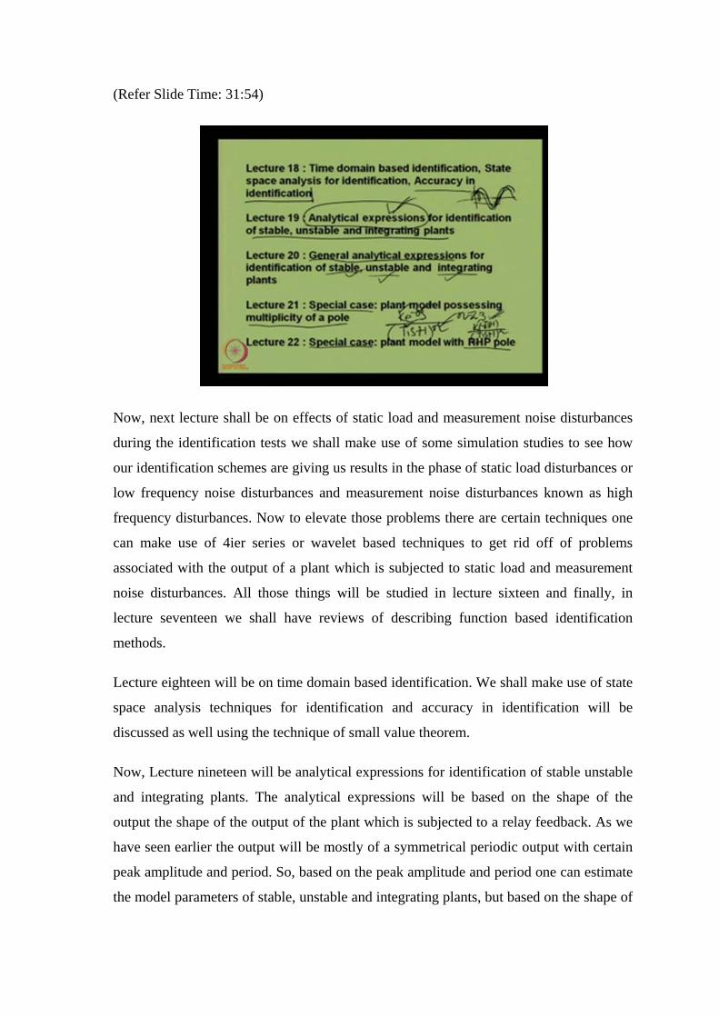
Now, next lecture shall be on effects of static load and measurement noise disturbances

during the identification tests we shall make use of some simulation studies to see how

our identification schemes are giving us results in the phase of static load disturbances or

low frequency noise disturbances and measurement noise disturbances known as high

frequency disturbances. Now to elevate those problems there are certain techniques one

can make use of 4ier series or wavelet based techniques to get rid off of problems

associated with the output of a plant which is subjected to static load and measurement

noise disturbances. All those things will be studied in lecture sixteen and finally, in

lecture seventeen we shall have reviews of describing function based identification

methods.

Lecture eighteen will be on time domain based identification. We shall make use of state

space analysis techniques for identification and accuracy in identification will be

discussed as well using the technique of small value theorem.

Now, Lecture nineteen will be analytical expressions for identification of stable unstable

and integrating plants. The analytical expressions will be based on the shape of the

output the shape of the output of the plant which is subjected to a relay feedback. As we

have seen earlier the output will be mostly of a symmetrical periodic output with certain

peak amplitude and period. So, based on the peak amplitude and period one can estimate

the model parameters of stable, unstable and integrating plants, but based on the shape of

the output one can also derive a number of analytical expression, those expressions can

be used further for estimation of the unknown plant model parameters. So, we shall make

use of state space analysis to obtain the analytical expressions based on the shape of the

output oscillatory output from the plants. Next we shall also derive a set of general

analytical expressions that can be made use of for identifying stable, unstable and

integrating plants. Why those are known as general analytical expressions, the analytical

expression need not be derived one each for stable or unstable or integrating plants rather

the same set of expressions with certain limiting values can be used to estimate the

unknown parameters.

Lecture twenty-one will be on special case like a plant having multiplicity of a Pole

which can be shown as ke to the power minus theta s T 1 s plus minus 1 to the power n

this is known as the plan model having multiplicity of poles where n can assume various

values starting from two three onwards.

So, we shall have a few more special cases on this when n equal two. When n equal to

three, what should be the analytical expressions and how we can solve the set of

analytical expressions using a certain non-linear equation solvers and find the unknowns

of the plant model parameters which are K theta T 1 and n. Again we shall deal with

another special case a plant model with right half plant pole which can again be shown as

k minus t zero s plus one upon t one s plus one to the power n. So, here this type of plant

model is supposed to have model with right half plant poles.


Next Lecture will also deal with a special case plant having complex conjugate poles. In

this case when the T 1 n T 2 we have been discussing so far, when they become complex

or complex numbers in that case the plant model are often given in the form of ke to the

power minus theta s a square plus b s plus one and. So, where b is such that we get under

damped action given or shown by these types of models. So, this is also falling under one

special case and we shall try to derive a set of analytical expressions for such cases.

Next we shall study estimation of dead time parameter of a transfer function model. A

second order transfer function model can have three to four unknowns, if some of the

unknowns can be estimated by some others technique then that will reduce the burden on

us in estimating the number of unknowns. It has been found that some other simple

techniques can be made use of to estimate some of the known unknowns of the second

order transfer function model. Dead time parameter which is often given as theta in all

Lectures can be estimated by some other techniques considering the output symmetrical

output of the plant subjected to relay feedback using some derivative of the output signal

and so on and zero crossings we can easily find this unknown parameter of the model

transfer functions. So, that will be discussed in Lecture twenty-four.

Lecture twenty-five will be on exactness of identification in the phase of measurement

noise and static load disturbances. So, accuracy of identification can be studied in this

Lecture.


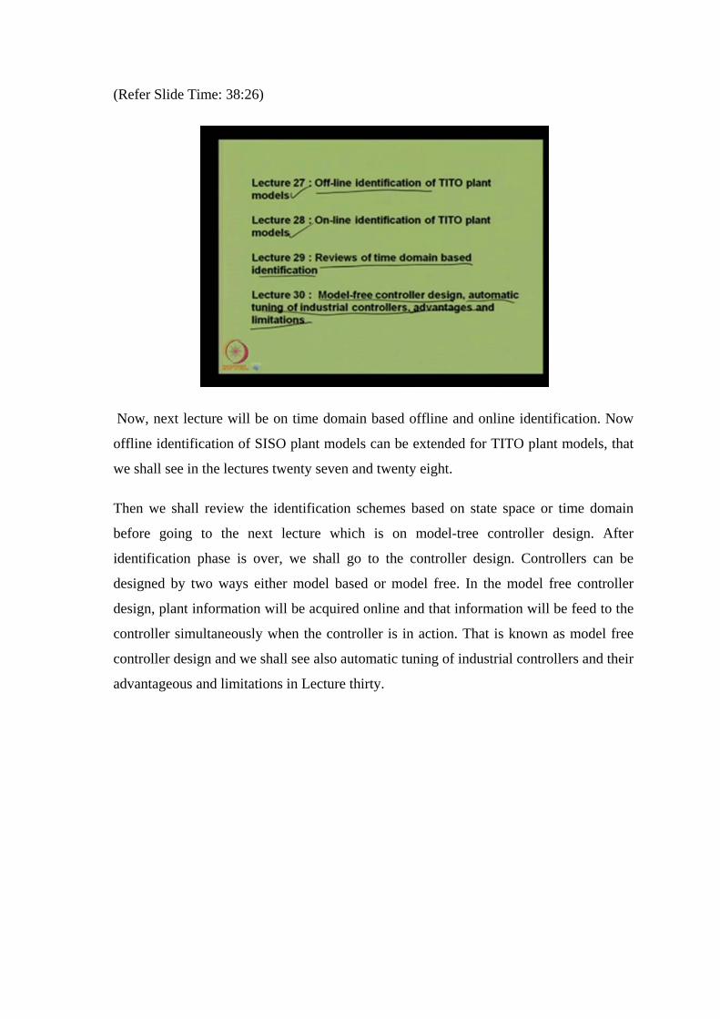
Now, next lecture will be on time domain based offline and online identification. Now

offline identification of SISO plant models can be extended for TITO plant models, that

we shall see in the lectures twenty seven and twenty eight.

Then we shall review the identification schemes based on state space or time domain

before going to the next lecture which is on model-tree controller design. After

identification phase is over, we shall go to the controller design. Controllers can be

designed by two ways either model based or model free. In the model free controller

design, plant information will be acquired online and that information will be feed to the

controller simultaneously when the controller is in action. That is known as model free

controller design and we shall see also automatic tuning of industrial controllers and their

advantageous and limitations in Lecture thirty.



Now, some advanced level of controllers to handle plants with long dead time known as

smith predictor controllers will be discussed in the three lectures, Lecture thirty-five,

thirty-six and thirty-seven. Here we shall present one Advanced Smith predictor

controller which can be used for controlling stable, unstable and intergrading plants.

The smith predictor controller can give us freedom to tune various controllers

independently. That is one of the benefits of the advanced smith predictor controller.

Standard form based controller design will be made use of while designing the

controllers of advanced smith predictor and controller. Standard forms based controller

design techniques have not drawn the attention it deserves. We shall show how simple

the technique is and how standard form based controller design can give better results

compared to some existing one. Then online controller of smith predictor control

structure also will be discussed employing relay in tandem with in tandem or in parallel

with the controller in Lecture thrity-seven.


In Lecture thirty-eight, we shall discuss about software and hardware implementation of

PID controller and its variants. Software implementation of PID controller is relatively

easy. Coming to the hardware implementation one can have analog PID controller,

digital controller and so on. Digital PID controllers can be effected with the help of many

processors, DSP processors, FPGA and so on whereas; analog PID controller can be

designed using field programmable analog arrays. We shall see in Lecture thirty-nine,

how in real time one can make use to field programmable analog arrays to design analog

PID controllers. There we shall also study how that is superior to field programmable

gate array based digital PID controllers.


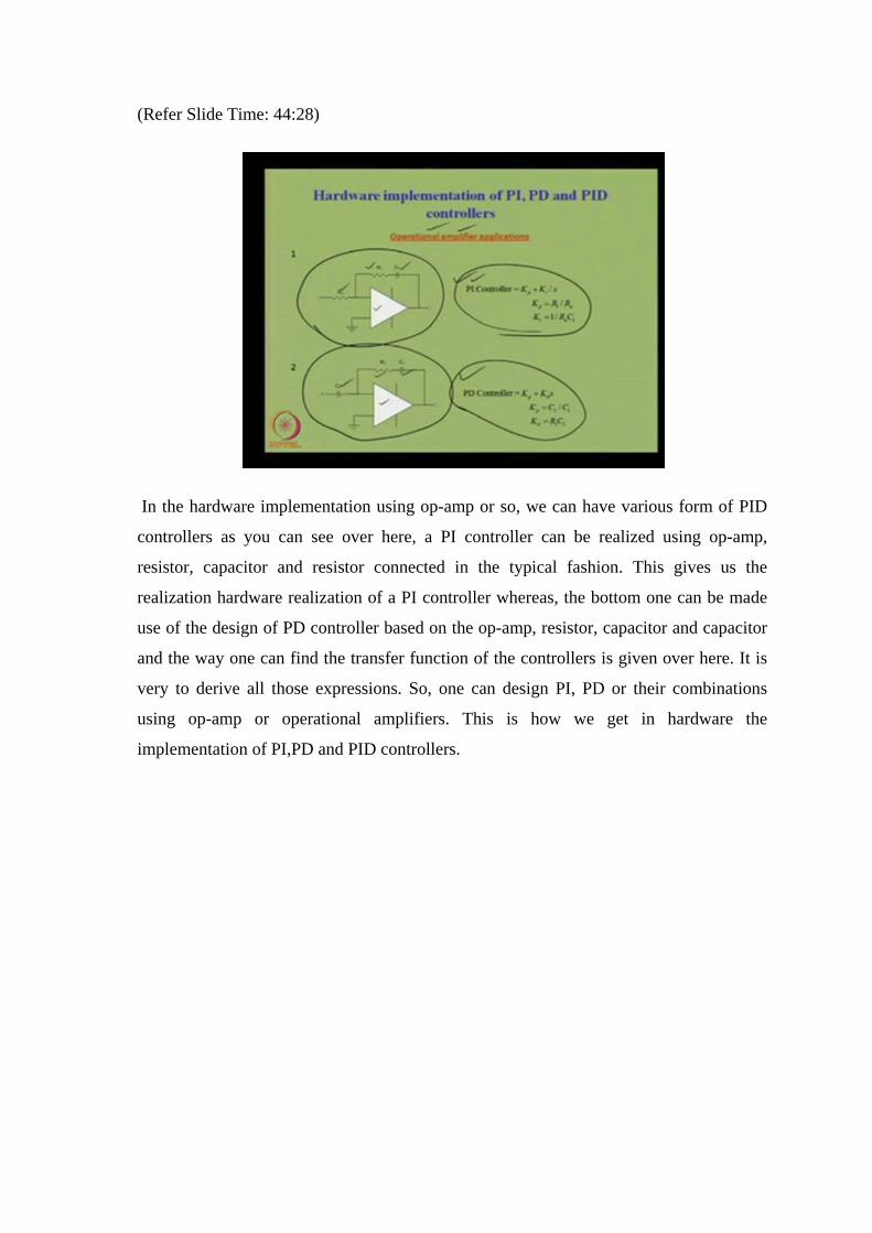
In the hardware implementation using op-amp or so, we can have various form of PID

controllers as you can see over here, a PI controller can be realized using op-amp,

resistor, capacitor and resistor connected in the typical fashion. This gives us the

realization hardware realization of a PI controller whereas, the bottom one can be made

use of the design of PD controller based on the op-amp, resistor, capacitor and capacitor

and the way one can find the transfer function of the controllers is given over here. It is

very to derive all those expressions. So, one can design PI, PD or their combinations

using op-amp or operational amplifiers. This is how we get in hardware the

implementation of PI,PD and PID controllers.


In FPAA field programmable analog array based controller design, one has to know the

structure of FPAA based controllers. So, one has to go through the modules given in the

package and then design FPAA based controllers. So here, this part actually gives us the

PID controller action and relay is shown over here. When relay is there, there are choices

to design offline and online PID controllers based on the acquired plant information.

Now that is all about the content of this course advanced control systems. In nutshell, it

can be summarized in this fashion what we are expected to learn from this course. First

of all, this course will introduce us certain classical control theory, PID controllers and

their limitation, PI-PD controller overcoming the structural limitations of PID controller.

Then we have also the control configurations for controlling two input two output

processes which can ultimately be extended to control of multi variable processes.

Now, next we shall learn in the course what a relay control system is and how that is

useful for identification of plant dynamics. Relay control using describing function

analysis and using state space analysis will be studied. Next we shall learn offline and

online identification of systems offline and online tuning of controllers. Lastly, we shall

learn how to implement controllers in real life and how real time controller can be

developed, how real time control systems can be developed. That is all about this course

Advanced Control Systems.

Advanced Control Systems Prof. Somanath Majhi Department of Electronics and Electrical

Documents

Transcript of Advanced Control Systems Prof. Somanath Majhi Department of Electronics and Electrical