Advanced Calculus: Lecture Notes for Mathematics 217-317sherm/m452/muldowney.pdf · ... Lecture...
189
“muldown 2010/1/10 page 1 ✐ ✐ ✐ ✐ ✐ ✐ ✐ ✐ Advanced Calculus: Lecture Notes for Mathematics 217-317 James S. Muldowney Department of Mathematical and Statistical Sciences The University of Alberta Edmonton, Alberta, Canada January 10, 2010
Transcript of Advanced Calculus: Lecture Notes for Mathematics 217-317sherm/m452/muldowney.pdf · ... Lecture...
“muldowney”2010/1/10page 1
i
i
i
i
i
i
i
i
Advanced Calculus: Lecture Notesfor Mathematics 217-317
James S. MuldowneyDepartment of Mathematical and Statistical Sciences
The University of Alberta
Edmonton, Alberta, Canada
January 10, 2010
“muldowney”2010/1/10page 2
i
i
i
i
i
i
i
i
2

“muldowney”2010/1/10page i
i
i
i
i
i
i
i
i
Contents
Preface iii
1 The Real Number system & Finite Dimensional Cartesian Space 11.1 The Real Number System R . . . . . . . . . . . . . . . . . . . . 1
1.1.1 Fields . . . . . . . . . . . . . . . . . . . . . . . . . . 11.1.2 Ordered Fields . . . . . . . . . . . . . . . . . . . . . 2Exercises . . . . . . . . . . . . . . . . . . . . . . . . . . . . . . . 31.1.3 Complete Ordered Field . . . . . . . . . . . . . . . . 41.1.4 Properties of R . . . . . . . . . . . . . . . . . . . . . 4Exercises . . . . . . . . . . . . . . . . . . . . . . . . . . . . . . . 5Exercises . . . . . . . . . . . . . . . . . . . . . . . . . . . . . . . 6
1.2 Cartesian Spaces . . . . . . . . . . . . . . . . . . . . . . . . . . . 71.2.1 Functions . . . . . . . . . . . . . . . . . . . . . . . . 11Exercises . . . . . . . . . . . . . . . . . . . . . . . . . . . . . . . 111.2.2 Convexity . . . . . . . . . . . . . . . . . . . . . . . . 13Exercises . . . . . . . . . . . . . . . . . . . . . . . . . . . . . . . 13
1.3 Topology . . . . . . . . . . . . . . . . . . . . . . . . . . . . . . . 13Exercises . . . . . . . . . . . . . . . . . . . . . . . . . . . . . . . 21
2 Limits, Continuity, and Differentiation 252.1 Sequences . . . . . . . . . . . . . . . . . . . . . . . . . . . . . . 25
Exercises . . . . . . . . . . . . . . . . . . . . . . . . . . . . . . . 29Exercises . . . . . . . . . . . . . . . . . . . . . . . . . . . . . . . 33
2.2 Continuity . . . . . . . . . . . . . . . . . . . . . . . . . . . . . . 352.3 Global Properties of Continuous Functions . . . . . . . . . . . . 38
Exercises . . . . . . . . . . . . . . . . . . . . . . . . . . . . . . . 422.4 Uniform Continuity . . . . . . . . . . . . . . . . . . . . . . . . . 42
Exercises . . . . . . . . . . . . . . . . . . . . . . . . . . . . . . . 442.5 Limits . . . . . . . . . . . . . . . . . . . . . . . . . . . . . . . . 462.6 Differentiation of real valued functions of a real variable . . . . . 49
Exercises . . . . . . . . . . . . . . . . . . . . . . . . . . . . . . . 52
3 Riemann Integration 573.1 Content and the Riemann Integral . . . . . . . . . . . . . . . . . 57
i
“muldowney”2010/1/10page ii
i
i
i
i
i
i
i
i
ii Contents
3.1.1 Partition of I . . . . . . . . . . . . . . . . . . . . . . 593.1.2 Riemann Sums . . . . . . . . . . . . . . . . . . . . . 59Exercises . . . . . . . . . . . . . . . . . . . . . . . . . . . . . . . 60
3.2 Cauchy Criteria and Properties of Integrals . . . . . . . . . . . . 61Exercises . . . . . . . . . . . . . . . . . . . . . . . . . . . . . . . 69
3.3 Evaluation of Integrals . . . . . . . . . . . . . . . . . . . . . . . 713.3.1 Real valued functions of a real variable . . . . . . . 713.3.2 Real valued functions on R2 . . . . . . . . . . . . . . 733.3.3 Real valued functions on Rn . . . . . . . . . . . . . 76Exercises . . . . . . . . . . . . . . . . . . . . . . . . . . . . . . . 77
4 Differentiation 0f Functions of Several Variables 814.1 Preliminaries . . . . . . . . . . . . . . . . . . . . . . . . . . . . . 81
4.1.1 Linear Functions . . . . . . . . . . . . . . . . . . . . 81Exercises . . . . . . . . . . . . . . . . . . . . . . . . . . . . . . . 844.1.2 Straight Lines and Curves . . . . . . . . . . . . . . . 85
4.2 The Directional Derivative and the Differential . . . . . . . . . . 86Exercises . . . . . . . . . . . . . . . . . . . . . . . . . . . . . . . 89Exercises . . . . . . . . . . . . . . . . . . . . . . . . . . . . . . . 964.2.1 Differentiation Rules . . . . . . . . . . . . . . . . . . 98Exercises . . . . . . . . . . . . . . . . . . . . . . . . . . . . . . . 102
4.3 Partial Derivatives of Higher Order . . . . . . . . . . . . . . . . 1054.3.1 Min-Max Theory . . . . . . . . . . . . . . . . . . . . 111Exercises . . . . . . . . . . . . . . . . . . . . . . . . . . . . . . . 119
4.4 Local Properties of C1 Functions . . . . . . . . . . . . . . . . . 124Exercises . . . . . . . . . . . . . . . . . . . . . . . . . . . . . . . 131
4.5 Implicit Function Theorem . . . . . . . . . . . . . . . . . . . . . 131Exercises . . . . . . . . . . . . . . . . . . . . . . . . . . . . . . . 1374.5.1 Dimension . . . . . . . . . . . . . . . . . . . . . . . 1394.5.2 Application: Lagrange Multipliers . . . . . . . . . . 147Exercises . . . . . . . . . . . . . . . . . . . . . . . . . . . . . . . 150
5 Further Topics in Integration 1555.1 Changes of Variables in Integrals . . . . . . . . . . . . . . . . . 155
Exercises . . . . . . . . . . . . . . . . . . . . . . . . . . . . . . . 1665.2 Integration on Curves and Surfaces . . . . . . . . . . . . . . . . 169
5.2.1 Curves (1-surfaces) . . . . . . . . . . . . . . . . . . . 1695.2.2 Surfaces (2-surfaces) . . . . . . . . . . . . . . . . . . 175Exercises . . . . . . . . . . . . . . . . . . . . . . . . . . . . . . . 178
“muldowney”2010/1/10page iii
i
i
i
i
i
i
i
i
Preface
These notes are not intended as a textbook. It is hoped however that theywill minimize the amount of notetaking activity which occupies so much of a stu-dent’s class time in most courses in mathmatics. Since the material is presented inthe sterile “definition, theorem, proof” form without much background colour ordiscussion most students will find it profitable to use the notes in conjunction witha textbook recommended by the instructor.
Probably the most important aspect of the notes is the set of exercises. Youshould develop the practice of attempting several of these problems every week.Many of the problems are quite difficult so please consult your instructor if youare not blessed with success initially. Do not acquire the habit of abandoning aproblem if it does not yield to your first attempt; a defeatist attitude is your greatestadversary. Solution of a problem, even with some assistance from the teacher whennecessary, is a fine boost to your morale. You will find that a strong effort expendedon the earlier part of the courses will be rewarded by growing self-confidence andeasier success later.
iii
“muldowney”2010/1/10page iv
i
i
i
i
i
i
i
i
iv Preface
NOTATION: Except when specified otherwise, upper case (capital) letters willdenote sets and lower case (small) letters will denote elements of sets.
a ∈ A means a is an element of the set A.
A ⊂ B means A is a subset of B.
a 6∈ A means a is NOT an element of the set A.
A 6⊂ B means A is NOT a subset of B.
Remark The slash through any symbol will mean the negation of the correspond-ing statement.
B ⊃ A means b contains A.
A ( B means A is a proper subset of B.
P =⇒ Q means statement P implies statement Q.
P ⇐⇒ Q means P holds if and only if Q holds.
∃ “there exists”.
∀ “for all”.
s.t. “such that”.
“end of proof”.
{x : . . .} means the set of all things x that satisfy conditions specified in . . .. Forexample, see the following.
A ∪B The union of sets A and B, {x : x ∈ A or x ∈ B}.
A ∩B The intersection of sets A and B, {x : x ∈ A and x ∈ B}.
A\B Set difference, {x : x ∈ A and x 6∈ B}.
A×B Cartesian product of sets A and B, {(x, y) : x ∈ A, y ∈ B}.
∅ The empty set, a set with no elements.
intervals For a, b ∈ R with a < b,
[a, b] means {x ∈ R : a ≤ x ≤ b} (closed interval).
(a, b) means {x ∈ R : a < x < b} (open interval).
(a, b] means {x ∈ R : a < x ≤ b}.
[a, b) means {x ∈ R : a ≤ x < b}.
“muldowney”2010/1/10page 1
i
i
i
i
i
i
i
i
Chapter 1
The Real Number system& Finite DimensionalCartesian Space
We begin by defining our basic tool, the real numbers R The real numbers canbe constructed from more primitive notions such as the natural numbers N :={1, 2, 3, . . .}, or even from the fundamental axioms of set theory. Here we shall becontent with a precise description of R.
1.1 The Real Number System R
Definition 1.1. R is a complete ordered field.
In the next several subsections we will explain the three underlined words.
1.1.1 Fields
A field is a set F together with two binary operations + and · (addition, multipli-cation) which satisfy the following axioms: For all a, b, c, . . . in F
F1 a+ b ∈ F and a · b ∈ F (closure)
F2 a+ b = b+ a and a · b = b · a (commutativity)
F3 a+ (b+ c) = (a+ b) + c and a · (b · c) = (a · b) · c (associativity)
F4 (a+ b) · c = (a · c) + (b · c) (distributivity)
F5 There exists unique elements 0 and 1 in F , 0 6= 1, such that
a+ 0 = a and a · 1 = a ∀ a ∈ F.
F6 For each a ∈ F , there exists −a ∈ F such that a+(−a) = 0, and if a 6= 0, thereexists a−1 ∈ F such that a · a−1 = 1 (existence of inverses).
Please note the following conventions and easy consequences:
1
“muldowney”2010/1/10page 2
i
i
i
i
i
i
i
i
2 Chapter 1. The Real Number system & Finite Dimensional Cartesian Space
1. a · b will henceforth be written ab.
2. a(b + c) = ab + ac is an consequence of axioms F2 and F4, and need not beseparately assumed. (verify for yourself)
3. The elements (−a) and a−1 are uniquely determined by a. Suppose, forexample, that there are two elements (−a1), (−a2) that satisfy a + (−a1) =0 = a+ (−a2). Then
(−a1) = (−a1)+0 = (−a1)+(a+(−a2)) = ((−a1)+a)+(−a2) = 0+(−a2) = (−a2).
4. It is customary to write a− b for a+ (−b) and ab for ab−1.
5. aa, aaa, . . . are usually denoted a2, a3, . . ..
6. {1, 1 + 1, 1 + 1 + 1, 1 + 1 + 1 + 1, . . .} is usually denoted {1, 2, 3, 4, . . .} = N.
Example 1.2 i The simplest (and least interesting) field is the set {θ, e} with
the operations+ θ eθ θ ee e θ
· θ eθ θ θe θ e
ii The set Q of rational numbers, i.e., numbers of the form mn (n 6= 0) with the
usual addition and multiplication is a field.
iii The sets R and C of real and complex numbers respectively with the usualaddition and multiplication are fields.
iv The set Q(t) of rational functions with rational coefficients (i.e. functions of
the form p(t)q(t) where p(t) and q(t) are polynomials with rational coefficients)
is a field.
v The set N = {1, 2, 3, 4, . . .} of natural numbers and the set Z of integers areNOT fields.
1.1.2 Ordered Fields
A field F is ordered if there is a subset P of F (called the positive elements) suchthat the following order axioms hold:
O1 a, b ∈ P =⇒ a+ b ∈ P and ab ∈ P .
O2 0 /∈ P
O3 x ∈ F, x 6= 0 =⇒ x ∈ P or − x ∈ P but not both.
“muldowney”2010/1/10page 3
i
i
i
i
i
i
i
i
1.1. The Real Number System R 3
Remark: Every ordered field contains Q as a subfield (we do not prove this). Thus,Q may be characterized as an ordered field containing no ordered proper subfield,i.e., Q is the smallest ordered field. (Two ordered fields are considered the same ifthey are isomorphic and the isomorphism preserves the order.) A discussion of thispoint may be found in
C. Goffman, Real Functions, Proposition 1 and 2 in Chapter 3.
E. Hewitt and K. Stromberg, Real and Abstract Analysis, Theorem 5.9.
We define a relation > on an ordered field as follows: If a, b ∈ F , write a > b(equivalently, b < a) if a − b ∈ P . Then the axioms O1, O2, and O3 have thefollowing consequences:
Proposition 1.3 (Properties of <).
i a > b, b > c implies a > c.
ii If a, b ∈ F , then exactly one of the following holds, a > b, b > a, a = b.
iii a ≥ b, b ≥ a implies a = b.
iv a > b implies a+ c > b+ c for each c ∈ F .
v a > b, c > d implies a+ c > b+ d.
vi a > b, c > 0 implies ac > bc and a > b, c < 0 implies ac < bc.
vii a > 0 implies a−1 > 0 and a < 0 implies a−1 < 0.
viii a > b implies a > a+b2 > b.
ix ab > 0 implies either a > 0 and b > 0, or a < 0 and b < 0.
Exercises
1.1. Establish the following properties of a field:
(a) a · 0 = 0
(b) a · (−1) = (−a)(c) (−a)(−b) = ab
(d) (ab−1)(cd−1) = ac(bd)−1
(f) If ab = 0, then a = 0 or b = 0.
1.2. Observe that for P being the set of positive elements
(a) 1 ∈ P(b) a 6= 0 =⇒ a2 ∈ P(c) If n ∈ N, then n ∈ P .
“muldowney”2010/1/10page 4
i
i
i
i
i
i
i
i
4 Chapter 1. The Real Number system & Finite Dimensional Cartesian Space
(d) The field {θ, e} in Example 1.2(i) cannot be ordered.
(e) The field C of complex numbers cannot be ordered.
(f) The fields Q and R are ordered by the usual notion of positivity.
(g) The field Q(t) in Example 1.2(iv) is ordered if p(t)q(t) ∈ P whenever the
highest power of t in the product p(t)q(t) is positive.
1.3. Prove the statements (i)-(ix) of Proposition 1.3.
1.1.3 Complete Ordered Field
The notion of completeness for an ordered field will stretch your imagination a littlefurther. We will introduce some terminology necessary to discuss this topic. Let Sbe a subset of an ordered field F .
(a) An element u ∈ F is an upper bound of the set S if s ≤ u, ∀s ∈ S.
(b) w ∈ F is a lower bound of S if w ≤ s, ∀s ∈ S.
(c) S is bounded above (below) if it has an upper (lower) bound in F . S is boundedif it is bounded above and below. For example, the set of natural numbers N
is bounded below and unbounded above; the interval [0, 1) = {x : 0 ≤ x < 1}is bounded.
(d) u is the least upper bound (or supremum) of S if
(i) s ≤ u, ∀s ∈ S, that is u is an upper bound, and
(ii) s ≤ v, ∀s ∈ S =⇒ u ≤ v, that is u is smaller than any other upperbound for S.
We write either u = supS or u = lubS.
(e) Similarly, the greatest lower bound (or infimum) of S is a number w which isa lower bound for S and exceeds all other lower bounds. We write w = inf Sor w = glbS.
Definition 1.4. An ordered field F is complete if each nonempty subset S of Fwhich has an upper bound has a least upper bound (supremum).
The only (to within an isomorphism) complete ordered field is R. Again wedo not prove this. A discussion may be found in the book of Hewitt and Stromberg,p.45.
1.1.4 Properties of R
The first property is for an ordered field F to be Archimedean:
Definition 1.5. An ordered field F is Archimedean if ∀a ∈ F , there exists n ∈ N ={{1, 2, 3, 4, . . .} such that n > a. (That is the set N is not bounded above.)
“muldowney”2010/1/10page 5
i
i
i
i
i
i
i
i
1.1. The Real Number System R 5
Theorem 1.6. R is Archimedean.
Proof. Suppose not. Then let a ≥ n, ∀n ∈ N be an upper bound of N. Then thereexists a least upper bound b = sup N, since R is complete. Thus, b ≥ n, ∀n ∈ N andb− 1 < n0 for some no ∈ N. But then, b < n0 + 1 ∈ N, contradicting b = supN.
Corollary 1.7. If a > 0, there exists n ∈ N such that 0 < 1n < a.
Proof. There exists n > a−1 > 0. (Why?). Thus, a > 1n > 0.
Corollary 1.8. Q is an Archimedean ordered field.
Corollary 1.9. If a, b ∈ R, a < b, then there is a rational r such that a < r < b.
Proof. There exists an n ∈ N such that n(b − a) > 1 (why?). Let m be the leastinteger such that m > na. Hence, m− 1 ≤ na and so
na < m ≤ na+ 1 < na+ n(b− a) = nb =⇒ a <m
n< b.
Exercises
1.3. Guess the supremum and infimum of the following sets (when they exist):(0, 1) = {x : 0 < x < 1} [0, 1] = {x : 0 ≤ x ≤ 1}{ 1n : n = 1, 2, 3, 4, . . .} N = {1, 2, 3, 4, . . .}
1.4. If a > 0, there exists n ∈ N such that 0 < 12n < a. Hint: Show 2n > n,
∀n ∈ N.
1.5. Q is not Archimedean.
1.6. Let F be an Archimedean ordered field containing an irrational element ξ.Show that if a, b ∈ F , a < b, then there is an irrational element η such thata < η < b.
1.7. Show that R contains an irrational element. Hint: Show first that no rationalp satisfies p2 = 2. Then show that p = sup{x > 0 : x2 < 2} must satisfyp2 = 2.
Theorem 1.10. Let In = [an, bn], and In+1 ⊂ In, n ∈ N. Then ∩∞n=1In 6= ∅. Inother words, a nested sequence of closed intervals has at least one point common toall intervals.
Proof. First note that an < bm for all n,m. Thus, each bm is an upper bound forthe set {an : n ∈ N}. Therefore, a := sup{an : n ∈ N} ≤ bm for all m. It followsthat an ≤ a ≤ bn for all n. Thus, a ∈ In for all n.
“muldowney”2010/1/10page 6
i
i
i
i
i
i
i
i
6 Chapter 1. The Real Number system & Finite Dimensional Cartesian Space
Definition 1.11. For x ∈ R, the absolute value |x| is defined via
|x| ={x, if x ≥ 0;−x. if x < 0.
The main properties of the absolute value are listed in
Proposition 1.12 (Properties of | · |). For x ∈ R, there holds
(i) |x| = 0⇐⇒ x = 0.
(ii) | − x| = |x|.
(iii) |xy| = |x| |y|.
(iv) If c ≥ 0, then |x| ≤ c⇐⇒ −c ≤ x ≤ c.
(v) ||a| − |b|| ≤ |a+ b| ≤ |a|+ |b|.
Proof. Part (i)–(iv) are an exercise.For the proof of (v), note
(iv) =⇒ −|a| ≤ a ≤ |a|, −|b| ≤ b ≤ |b|=⇒ −(|a|+ |b|) ≤ a+ b ≤ |a|+ |b|
(iv) =⇒ |a+ b| ≤ |a|+ |b|
which is the desired right hand inequality. This implies the left hand inequalitysince
|b| = |b− a+ a| ≤ |b− a|+ |a| =⇒ |b| − |a| ≤ |b− a| = |a− b|,interchanging a and b =⇒ |a| − |b| ≤ |a− b|,=⇒ ||a| − |b|| ≤ |a− b| by definition of | · |.
The rest of (v) follows from replacing b by −b.
Exercises
1.9. Let F be an ordered field, with the property that if {In} is a nested sequenceof closed intervals in F , then ∩∞n=1In 6= ∅. Show that F is complete. (Remark:This exercise and Theorem 1.10 shows that the supremum (completeness)property and the nested interval property are equivalent.)
1.10. Let In = (0, 1n ). Show that ∩∞n=1In = ∅.
1.11. Let Kn = [n,∞) := {x : x ≥ n}. Show that ∩∞n=1Kn = ∅.
“muldowney”2010/1/10page 7
i
i
i
i
i
i
i
i
1.2. Cartesian Spaces 7
1.12. If a set S of real numbers contains one of its upper bounds a, then a = supS.Such a supremeum is called a maximum.
1.13. Show that S ⊂ R cannot have two suprema.
1.14. Show that an ordered field F is complete if and only if every non-emptysubset of F which has a lower bound has an infimum.
1.15. Show that Q is not complete.
1.16. If s ⊂ R is bounded and S0 ⊂ S, show
inf S ≤ inf S0 ≤ supS0 ≤ supS.
1.17. If S = {(−1)n(1− 1n ) : n = 1, 2, . . .}, find supS, inf S. Prove any statements
you make.
1.18. Prove (i) – (iv) of Proposition 1.12.
1.2 Cartesian Spaces
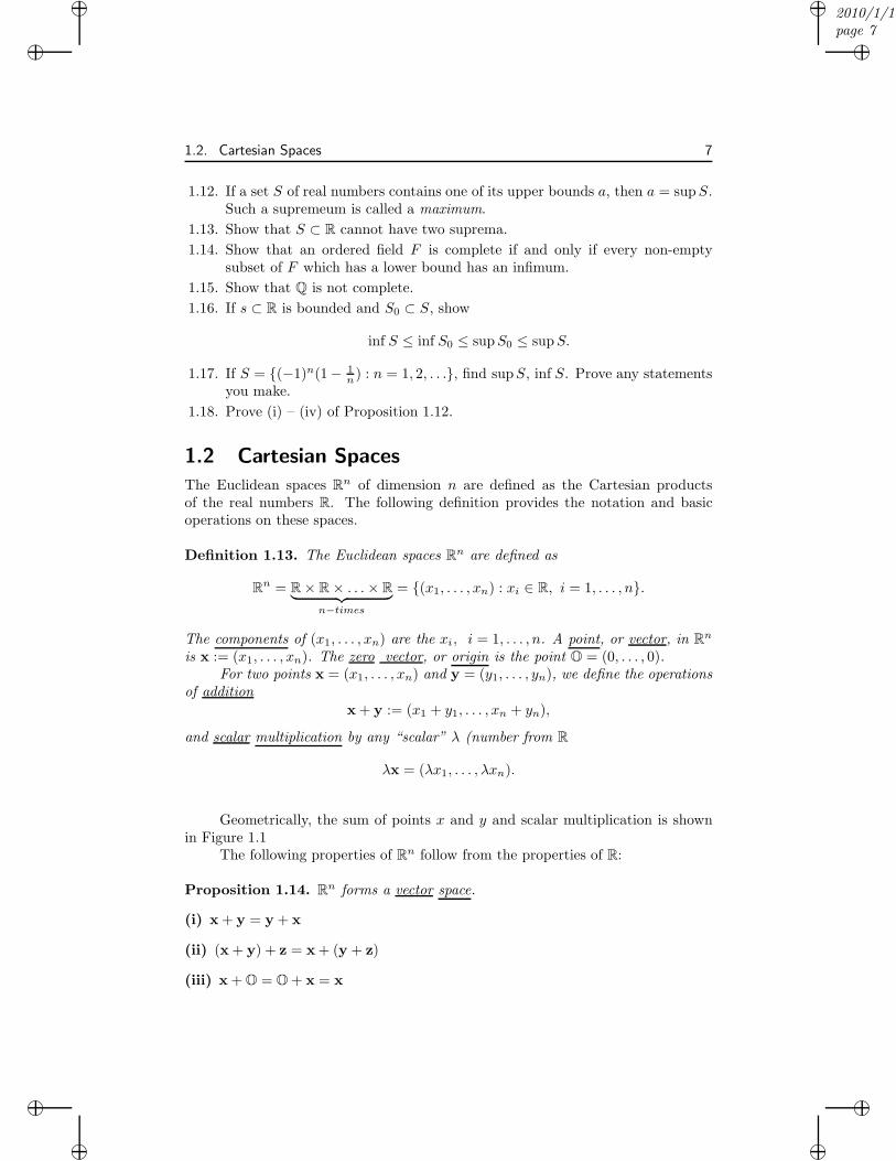
The Euclidean spaces Rn of dimension n are defined as the Cartesian productsof the real numbers R. The following definition provides the notation and basicoperations on these spaces.
Definition 1.13. The Euclidean spaces Rn are defined as
Rn = R× R× . . .× R︸ ︷︷ ︸n−times
= {(x1, . . . , xn) : xi ∈ R, i = 1, . . . , n}.
The components of (x1, . . . , xn) are the xi, i = 1, . . . , n. A point, or vector, in Rn
is x := (x1, . . . , xn). The zero vector, or origin is the point O = (0, . . . , 0).For two points x = (x1, . . . , xn) and y = (y1, . . . , yn), we define the operations
of addition
x + y := (x1 + y1, . . . , xn + yn),
and scalar multiplication by any “scalar” λ (number from R
λx = (λx1, . . . , λxn).
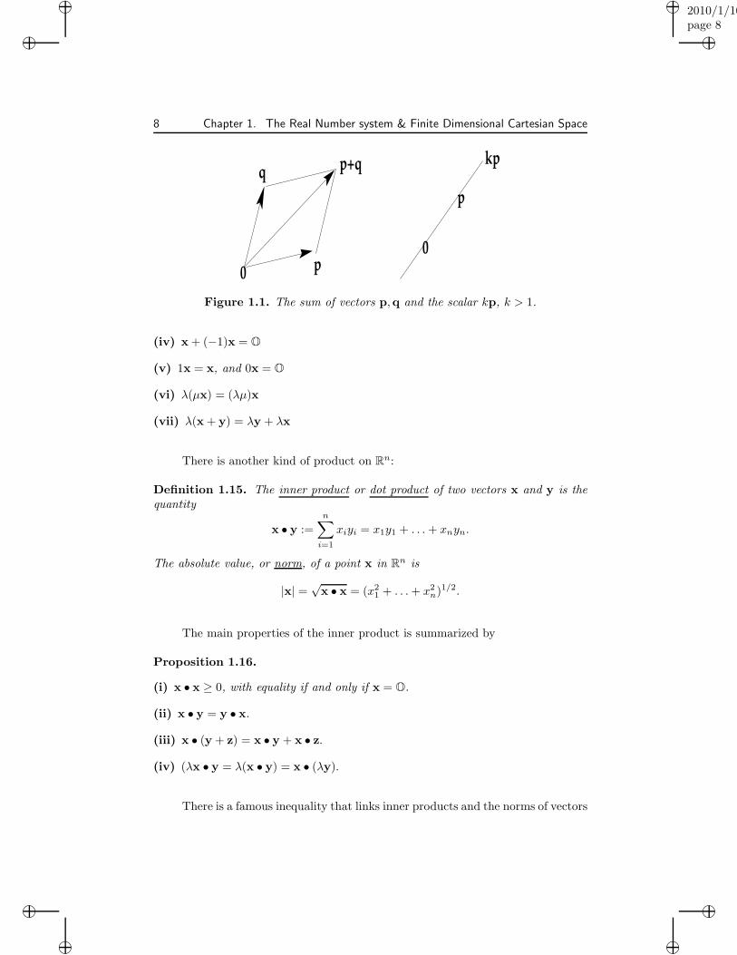
Geometrically, the sum of points x and y and scalar multiplication is shownin Figure 1.1
The following properties of Rn follow from the properties of R:
Proposition 1.14. Rn forms a vector space.
(i) x + y = y + x
(ii) (x + y) + z = x + (y + z)
(iii) x + O = O + x = x
“muldowney”2010/1/10page 8
i
i
i
i
i
i
i
i
8 Chapter 1. The Real Number system & Finite Dimensional Cartesian Space
p
p+q
0
p
kp
0
q
Figure 1.1. The sum of vectors p,q and the scalar kp, k > 1.
(iv) x + (−1)x = O
(v) 1x = x, and 0x = O
(vi) λ(µx) = (λµ)x
(vii) λ(x + y) = λy + λx
There is another kind of product on Rn:
Definition 1.15. The inner product or dot product of two vectors x and y is thequantity
x • y :=
n∑
i=1
xiyi = x1y1 + . . .+ xnyn.
The absolute value, or norm, of a point x in Rn is
|x| =√
x • x = (x21 + . . .+ x2
n)1/2.
The main properties of the inner product is summarized by
Proposition 1.16.
(i) x • x ≥ 0, with equality if and only if x = O.
(ii) x • y = y • x.
(iii) x • (y + z) = x • y + x • z.
(iv) (λx • y = λ(x • y) = x • (λy).
There is a famous inequality that links inner products and the norms of vectors
“muldowney”2010/1/10page 9
i
i
i
i
i
i
i
i
1.2. Cartesian Spaces 9
Theorem 1.17 (Cauchy-Bunyakowski-Schwarz inequality). For all x,y ∈Rn, we have
x • y ≤ |x| |y|,with equality if and only if either one of x,y is O, or x = λy with λ > 0.
Proof. Let z = λx− µy with λ, µ ∈ R. From the properties of inner products, wehave
0 ≤ z • z by (i)
= λ2x • x− 2λµx • y + µ2y • y, by (ii), (iii) and (iv)
= |y|2|x|2 − 2|x||y|x • y + |x|2|y|2, choosing λ = |y|, µ = |x|= 2|x| |y| [|x| |y| − x • y] .
Hence, x • y ≤ |x| |y|. If equality holds in the last expression, then working back-wards through the proof yields
O = z = |y|x − |x|y, i.e. x =|x||y|y.
Corollary 1.18. For all x,y ∈ Rn, we have
|x • y| ≤ |x| |y|,
or
|x1y1 + . . .+ xnyn| ≤(x2
1 + . . .+ x2n
)1/2(y21 + . . .+ y2
n
)1/2
.
Corollary 1.19 (Triangle Inequality).
||x| − |y|| ≤ |x± y| ≤ |x|+ |y|.
Proof. We have
|x + y|2 = (x + y) • (x + y) = x • x + 2x • y + y • y= |x|2 + 2x • y + |y|2≤ |x|2 + 2|x| |y|+ |y|2, (CBS inequality)
=(|x|+ |y|
)2
=⇒ |x + y| ≤ |x|+ |y|.
The left-hand inequality follows from this just as in the scalar triangle inequality.
Proposition 1.20 (Properties of Norm).
“muldowney”2010/1/10page 10
i
i
i
i
i
i
i
i
10 Chapter 1. The Real Number system & Finite Dimensional Cartesian Space
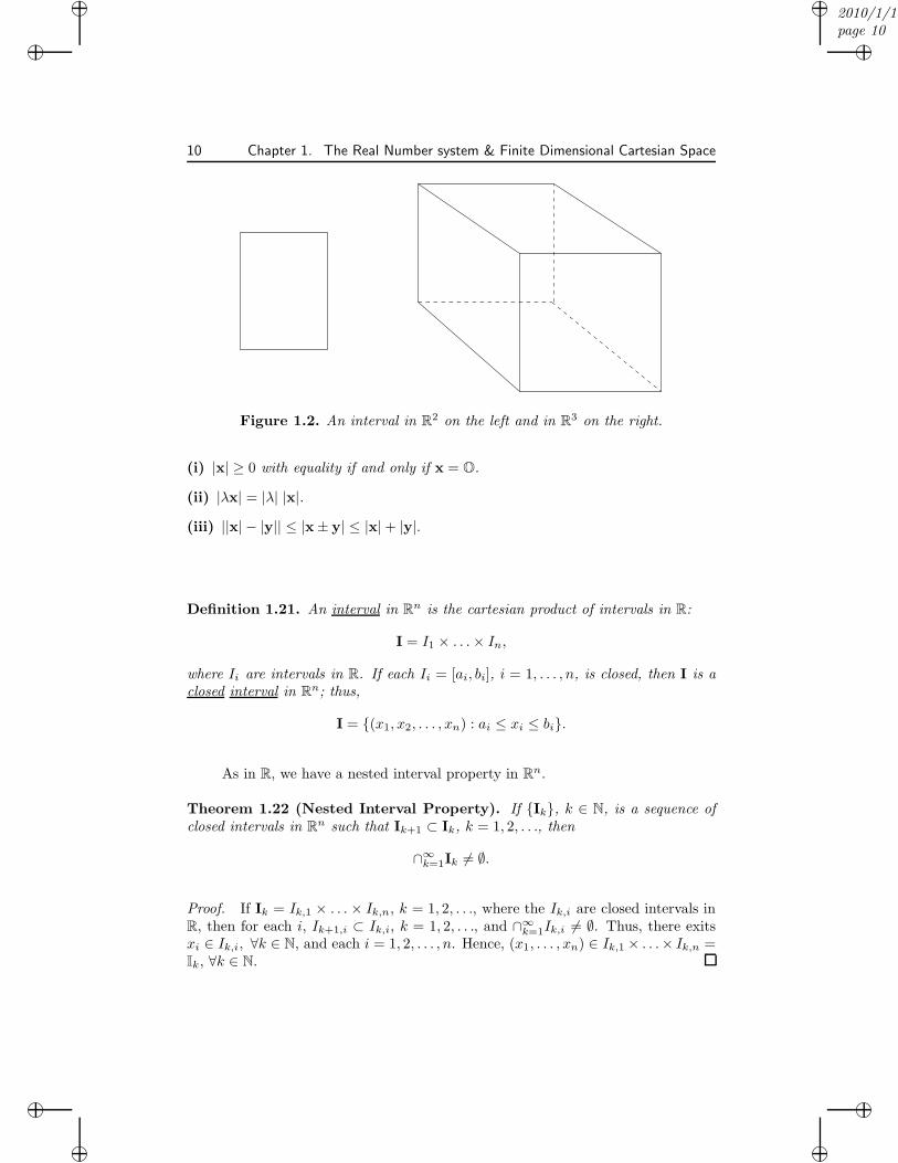
Figure 1.2. An interval in R2 on the left and in R3 on the right.
(i) |x| ≥ 0 with equality if and only if x = O.
(ii) |λx| = |λ| |x|.
(iii) ||x| − |y|| ≤ |x± y| ≤ |x|+ |y|.
Definition 1.21. An interval in Rn is the cartesian product of intervals in R:
I = I1 × . . .× In,
where Ii are intervals in R. If each Ii = [ai, bi], i = 1, . . . , n, is closed, then I is aclosed interval in Rn; thus,
I = {(x1, x2, . . . , xn) : ai ≤ xi ≤ bi}.
As in R, we have a nested interval property in Rn.
Theorem 1.22 (Nested Interval Property). If {Ik}, k ∈ N, is a sequence ofclosed intervals in Rn such that Ik+1 ⊂ Ik, k = 1, 2, . . ., then
∩∞k=1Ik 6= ∅.
Proof. If Ik = Ik,1 × . . . × Ik,n, k = 1, 2, . . ., where the Ik,i are closed intervals inR, then for each i, Ik+1,i ⊂ Ik,i, k = 1, 2, . . ., and ∩∞k=1Ik,i 6= ∅. Thus, there exitsxi ∈ Ik,i, ∀k ∈ N, and each i = 1, 2, . . . , n. Hence, (x1, . . . , xn) ∈ Ik,1 × . . .× Ik,n =Ik, ∀k ∈ N.
“muldowney”2010/1/10page 11
i
i
i
i
i
i
i
i
1.2. Cartesian Spaces 11
1.2.1 Functions
Definition 1.23. A subset f of A×B is a function from A to B if
(x, y1), (x, y2) ∈ f =⇒ y1 = y2.
We write f : A 7→ B, (“f is a function from A to B). For (x, y) ∈ f , we use thenotation y = f(x). The set Rf := {y : (x, y) ∈ f} for some x is called the rangeof f , and the set Df := {x : (x, y) ∈ f for some y } is called the domain of f . IfU ⊂ A, then f(U) := {f(x) : x ∈ U} is called the image of U . If V ⊂ B, then
f−1(V ) := {x : f(x) ∈ V } is called the inverse image of V .
Example 1.24 Consider f = {(x, x2) : −1 ≤ x ≤ 1}; the function f(x) = x2.Then
Df = [−1, 1] Rf = [0, 1]
f([−1, 1/2]
)= [0, 1] f−1
([−1, 1/2]
)= [0, 1/
√2].
Definition 1.25. A function f : A 7→ B is one-to-one if it also satisfies
(x1, y), (x2, y) ∈ f =⇒ x1 = x2.
We write this f :1−17→ B.
Note that if f :1−17→ B, then {(y, x) : (x, y) ∈ f} is also a one-to-one function,
which is denoted by f−1 : B1−17→ A, and is called the inverse function of f .
If f : A 7→ B and g : B 7→ C are two functions, then the composition of gwith f is the function
g ◦ f(x) = g(f(x)) with domain given by Dg◦f = f−1(Dg).
Example 1.26 As an example of a composition,f : R 7→ R2 f(x) = (|x|, x2 + 1)g : R2 7→ R2 g(u, v) = (u+ v, u − v)g ◦ f : R 7→ R2 g ◦ f(x) = (|x|+ x2 + 1, |x| − x2 − 1).
Exercises
1.19. Prove Corollary 1.18.
1.20. Show |x + y|2 + |x − y|2 = 2(|x|2 + |y|2) for all x,y ∈ Rn. (parallelogramidentity)
1.21. If x = (x1, . . . , xn), show
|xi| ≤ |x ≤√n sup{|x1|, . . . , |xn|}, for i = 1, . . . , n.
“muldowney”2010/1/10page 12
i
i
i
i
i
i
i
i
12 Chapter 1. The Real Number system & Finite Dimensional Cartesian Space
1.22. Show that |x+y|2 = |x|2 + |y|2 ⇐⇒ x •y = 0. In this case, x and y are saidto be orthogonal. This is sometimes denoted by x ⊥ y.
1.23. Is it true that
|x + y| = |x|+ |y| ⇐⇒ x = λy or y = λx with λ ≥ 0?
1.24. Two sets A and B have the same cardinality if there is a one-to-one function
φ : A 7→ B such that φ(A) = B and φ−1(B) = A. Show that the followingsets have the same cardinality:
(a) N = {1, 2, 3, . . .} and 2N = {2, 4, 6, 8, . . .}.(b) [0, 1] and [0, 2].
(c) (0, 1) and (0,∞) = {x : x > 0}.(d) [0, 1] and [0, 1).
1.25. A set A is said to be finite if it has the same cardinality as some initial segment{1, . . . , n} of the natural numbers, and is said to be infinite otherwise. (Thus,finite means that the elements can be labeled a1, . . . , an.) Show that a finiteset of real numbers contains its inf and its sup. Hint: Induction.
1.26. A set A is countable if it has the same cardinality as N, the set of naturalnumbers, or if it is finite. Otherwise, the set is said to be uncountable. Showthat a countable set need not contain its sup or its inf. (Countability meansall elements of the set can be labeled by the natural numbers {a1, a2, a3, . . .}.)
1.27. Show that the union of a countable collection of countable sets is countable.Hint:
S1 : a1,1 → a1,2 a1,3 → . . .ւ ր ւ
S2 : a2,1 a2,2 a2,3 . . .↓ ր ւ ր
S3 : a3,1 a3,2 a3,3, . . .ւ ր ւ
S4 : a4,1 a4,2 a4,3, . . .... :
......
......
......
...
The elements may be counted by the scheme indicated . Deduce that Q iscountable.
1.28. [0, 1] is uncountable. Complete this sketch of proof: Suppose [0, 1] is count-able and that
[0, 1] = {a1, a2, . . .}.At least one of the intervals [0, 1
3 ], [ 13 ,23 ], [23 , 1] does not contain a1; call this
interval I1. Subdivide I1 into three closed intervals, then a2 in not in one ofthose three; call it I2. Continuing in this manner, we obtain a nested sequenceof closed intervals, In, with the property that an 6∈ In. Therefore, none ofthe an are in ∩∞k=1Ik. But, by the nested interval theorem, the intersectionis non-empty so there must be an x ∈ [0, 1] with x 6= an for any n. Thiscontradicts our assumption.
“muldowney”2010/1/10page 13
i
i
i
i
i
i
i
i
1.3. Topology 13
1.2.2 Convexity
Definition 1.27. For two points x,y ∈ Rn with x 6= y, we define
(i) the line through x and y as {x + t(y − x) : t ∈ R};(ii) and the line segment between x and y as the set {x + t(y − x) : t ∈ [0, 1]}.A subset C of Rn is convex if
x,y ∈ C =⇒ x + t(y − x) ∈ C, ∀t ∈ [0, 1];
that is, if the line segment between any two points of the set is a subset of C.
Example 1.28 S := {x : |x| ≤ 1} is convex.Proof. If |x| ≤ 1 and |y| ≤ 1, then
|x + t(y − x)| = |(1− t)x + ty| ≤ |(1− t)x|+ |ty|. triangle inequality
≤ (1− t)|x|+ t|y| ≤ (1− t) + t = 1.
Thus, x + t(y − x) ∈ S, for 0 ≤ t ≤ 1; that is S is convex.
Exercises
1.29. Prove that {x : |x| = 1} is not convex.
1.30. Prove that {(x, y) ∈ R2 : y > 0} is convex.
1.31. Let C be any collection of convex sets. Show that ∩A∈CA is convex. Is ∪A∈CAnecessarily convex?
1.32. The convex hull H(A) of a set A is the intersection of all convex sets con-taining A as a subset. Prove that H(A) is convex. What is H(A) if A is aset consisting of two points only?
1.33. A subset C of Rn is a cone if {tx : x ∈ C} ⊂ C for all t ≥ 0.
(i) Prove that a cone C is a convex set if and only if
{x + y : x ∈ C, y ∈ C} ⊂ C.
(ii) Draw pictures of convex and non-convex cones in R2.
1.3 Topology
Definition 1.29. If ρ > 0 and x0 ∈ Rn, then the open ball of center x0 and radiusρ is the set
B(x0, ρ) := {x : |x− x0| < ρ}.A neighborhood of x0 is any set U which contains an open ball with center x0 as asubset.A set A is open in Rn if it is a neighborhood of each of its points.
“muldowney”2010/1/10page 14
i
i
i
i
i
i
i
i
14 Chapter 1. The Real Number system & Finite Dimensional Cartesian Space
Example 1.30 Consider the following examples:
1. Rn is open.
2. ∅ is open.
3. (0, 1) is open in R.
4. [0, 1) is not open in R.
5. {(x, y) : 0 < x < 1, y = 1} is not open in R2
6. B(x0, ρ) is open in Rn
Proof. (1),(2) and (5) are left to the reader. For (3) note that if x0 ∈ (0, 1), thenB(x0, δ) = (x0 − δ, x0 + δ) ⊂ (0, 1) when δ = min(x0, 1− x0).
For (4), note that B(0, δ) = (−δ, δ) is not in [0, 1) for any δ > 0.Finally, to see (6), let x1 ∈ B(x0, ρ). We will show that B(x1, ρ1) ⊂ B(x0, ρ)
when ρ1 = ρ−|x1−x0| > 0, so that B(x0, ρ) is a neighborhood of each of its points,and hence is open. Let x ∈ B(x1, ρ1), then
|x− x0| = |x− x1 + x1 − x0|≤ |x− x1|+ |x1 − x0| (triangle inequality)
< ρ1 + |x1 − x0| (p ∈ B(x1, ρ1))
= ρ− |x1 − x0|+ |x1 − x0| definition of ρ1
= ρ.
Thus, x ∈ B(x0, ρ), and also B(x1, ρ1) ⊂ B(x0, ρ).
Proposition 1.31 (Open set properties). For open sets in Rn, we have
(a) ∅ and Rn are open.
(b) If A and B are open sets, then A ∩B is an open set.
(c) The union of any collection of open sets is open.
Proof. For (a), note that both ∅ and Rn are neighborhoods of their points (for ∅,it is true because there are no points).
For (b), let x0 ∈ A ∩B. Then
x0 ∈ A =⇒ ∃ρ1 s.t. B(x0, ρ1) ⊂ A, (since A is open)
x0 ∈ B =⇒ ∃ρ2 s.t. B(x0, ρ2) ⊂ B, (since B is open)
=⇒ B(x0, ρ) ⊂ A and B(x0, ρ) ⊂ B for ρ = min(ρ1, ρ2)
=⇒ B(x0, ρ) ⊂ A ∩B=⇒ A ∩B is open.
“muldowney”2010/1/10page 15
i
i
i
i
i
i
i
i
1.3. Topology 15
For (c) let C be a collection of open sets, and select any x ∈ ∪A∈CA. Then
x ∈ A for some A ∈ C=⇒ B(x, ρ) ⊂ A for some ρ > 0 (A is open)
=⇒ B(x, ρ) ∈ ∪A∈CA
=⇒ ∪A∈CA is open
Definition 1.32. A set A is closed in Rn if its complement
Ac := Rn\A := {x ∈ Rn : x 6∈ A}
is an open set.
Proposition 1.33 (Properties of closed sets.).
(a) ∅ and Rn are closed.
(b) If A and B are closed sets, then A ∪B is a closed set.
(c) The intersection of any collection of closed sets is closed.
Example 1.34 Consider the following examples:
1. [0,∞) := {x : x ≥ 0} is closed in R. (Thus, (−∞, 0) is open.)
2. [0, 1] is closed in R, i.e. (−∞, 0) ∪ (1,∞) is open.
3. [0, 1) is not closed in R. (Why?)
4. {x : |x| ≥ 1} is closed in Rn. (Since B(O, 1) is open.)
5. {x : |x| ≤ 1} is closed in Rn. (Exercise.)
Proposition 1.35. For a closed set C and an open set V in Rn
(a) C\V is closed;
(b) V \C is open.
Proof. For (a) note that
C\V := {x : x ∈ C and x 6∈ V } = C ∩ V c.
which is closed since C and V c are closed.Part (b) is an exercise.
“muldowney”2010/1/10page 16
i
i
i
i
i
i
i
i
16 Chapter 1. The Real Number system & Finite Dimensional Cartesian Space
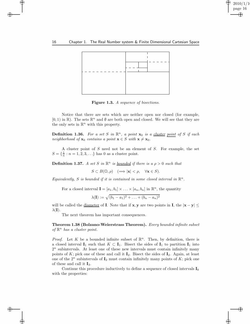
Figure 1.3. A sequence of bisections.
Notice that there are sets which are neither open nor closed (for example,[0, 1) in R). The sets Rn and ∅ are both open and closed. We will see that they arethe only sets in Rn with this property.
Definition 1.36. For a set S in Rn, a point x0 is a cluster point of S if eachneighborhood of x0 contains a point x ∈ S with x 6= x0.
A cluster point of S need not be an element of S. For example, the setS = { 1
n : n = 1, 2, 3, . . .} has 0 as a cluster point.
Definition 1.37. A set S in Rn is bounded if there is a ρ > 0 such that
S ⊂ B(O, ρ) (=⇒ |x| < ρ, ∀x ∈ S).
Equivalently, S is bounded if it is contained in some closed interval in Rn.
For a closed interval I = [a1, b1]× . . .× [an, bn] in Rn, the quantity
λ(I) :=√
(b1 − a1)2 + . . .+ (bn − an)2
will be called the diameter of I. Note that if x,y are two points in I, the |x− y| ≤λ(I).
The next theorem has important consequences.
Theorem 1.38 (Bolzano-Weierstrass Theorem). Every bounded infinite subsetof Rn has a cluster point.
Proof. Let K be a bounded infinite subset of Rn. Then, by definition, there isa closed interval I1 such that K ⊂ I1. Bisect the sides of I1 to partition I1 into2n subintervals. At least one of these new intervals must contain infinitely manypoints of K; pick one of these and call it I2. Bisect the sides of I2. Again, at leastone of the 2n subintervals of I2 must contain infinitely many points of K; pick oneof these and call it I3.
Continue this procedure inductively to define a sequence of closed intervals Ikwith the properties:
“muldowney”2010/1/10page 17
i
i
i
i
i
i
i
i
1.3. Topology 17
1. Each Ik contains infinitely many points of K.
2. 0 < λ(Ik) = 12k−1 λ(I1), k = 1, 2, 3, . . ..
3. There is a point x0 ∈ ∩kIk 6= ∅ by Theorem 1.10.
We must show that x0 is a cluster point of K. If this were not true, then therewould be a radius ρ > 0 such that the ball B(x0, ρ) does not intersect K:
B(x0, ρ) ∩K = ∅.
Now, choose k so that
0 <1
2k−1λ(I1) < ρ. Why is this possible?
Then 0 < λ(Ik) < ρ. Remember that for any x ∈ Ik, |x− x0| < λ(Ik) < ρ since x0
is also in Ik. Thus, Ik ⊂ B(x0, ρ). But, Ik contains (infinitely many) points of K;a contradiction. Therefore, x0 is a cluster point of K
Theorem 1.39. A subset K of Rn is closed if and only if K contains all of itscluster points.
Proof. “=⇒” Let K be closed. Let x0 be a cluster point of K. If x0 6∈ K, then x0
is in the open set Kc. Since Kc is open, there exists ρ > 0 so that B(x0, ρ) ⊂ Kc.That contradicts the definition of x0 being a cluster point of K. Hence, xo ∈ K.
“⇐=” Let K contain all of its cluster points. If x1 ∈ Kc, then x1 6∈ K, andis not a cluster point of K. Therefore, by definition of cluster points, there existsρ > 0 such that B(x1, ρ) ⊂ Kc. Thus, Kc is open and K is closed.
Definition 1.40. A collection G of open sets is an open cover of a set K if
K ⊂ ∪U∈GU.
A set K is Rn is compact if every open cover of K has a finite subcover; that is, forany open cover G, there is a finite collection of sets U1, . . . , Um from G such that
K ⊂ ∪mj=1Uj .
Some simple examples:
Example 1.41 The following examples illustrate the concept of compactness:
1. A finite set is compact.
2. [0,∞) is not compact. Indeed, the sets Gk := (−1, k), k ∈ N form an opencover of [0,∞), but there cannot be a finite subcover. (Why?)
“muldowney”2010/1/10page 18
i
i
i
i
i
i
i
i
18 Chapter 1. The Real Number system & Finite Dimensional Cartesian Space
3. (0, 1) is not compact. (Find the infinite open cover that does not have a finitesubcover.)
The next theorem is a very important characterization of compact subsets ofRn.
Theorem 1.42 (Heine-Borel Theorem). A subset K ofRn is compact iff and only if K is closed and bounded.
Proof. “=⇒” Let K be compact.We first show K is closed. Let x0 be any point in Kc. We wish to find a ball
B(x0, ρ) ⊂ Kc for some ρ. Then Kc would be open, and hence, K would be closed.Consider the collection G of open sets Gk, k ∈ N, where
Gk := {x : |x− x0| >1
k}.
(Why is Gk open?) Clearly, the collection G covers all of Rn\{x0}, and hence coversK. Since K is compact, there is a finite subcover {Gki
: i = 1, . . . ,m} of K. Now,the Gj are nested with Gj ⊂ Gi if i > j. Hence, letting k0 = max{k1, . . . , km}, wehave K ⊂ Gk0 . In other words,
B(x0,1
k0) := {x : |x− x0| <
1
k0} ⊂ {x : |x− x0| ≤
1
k0} = Gck0 ⊂ Kc.
Hence, Kc is open and K is closed.To show that K is bounded, consider the open cover consisting of all balls
B(O, k), k ∈ N. This collection covers all of Rn, and so is an open cover of K.Therefore, there is a finite subcover {B(O, ki : i = 1, . . . ,m} of K. Hence, K ⊂B(O, k0) where k0 := max{k1, . . . , km}. Thus, K is bounded.
“⇐=” Let K be closed and bounded. The proof will be by contradiction. If Kis not compact, then there exists an open cover G = {Gα} of K such that K is notcontained in any union of finitely many Gα’s. Since K is bounded, it is contained insome closed interval I1 in Rn. Bisect the sides of I1 to obtain 2n subintervals (as inthe proof of the Bolzano-Weierstrass Theorem). At least one of these subintervalsintersects K in such a way that this intersection cannot be covered by finitely manyGα’s. Select such a subinterval as I2. Proceeding inductively in this way, we obtaina nested sequence of closed intervals Ik, k = 1, 2, . . ., such that
1. Each K ∩ Ik cannot be covered by finitely many Gα’s, k = 1, 2, . . ..
2. λ(Ik) = λ(I1)/2k−1, k = 1, 2, . . ..
By the Nested Intervals Theorem, there is a point x0 ∈ ∩kIk, and this point is acluster point of K (as in the Bolzano-Weierstrass Theorem’s proof). Since K isclosed, x0 ∈ K. Therefore, x0 ∈ Gα0
for some α0, since the Gα cover K. But, Gα0
“muldowney”2010/1/10page 19
i
i
i
i
i
i
i
i
1.3. Topology 19
A
B
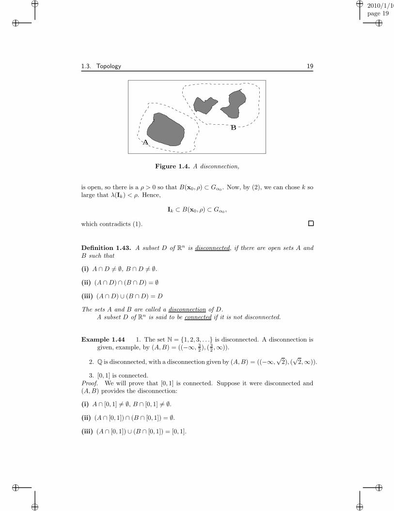
Figure 1.4. A disconnection,
is open, so there is a ρ > 0 so that B(x0, ρ) ⊂ Gα0. Now, by (2), we can chose k so
large that λ(Ik) < ρ. Hence,
Ik ⊂ B(x0, ρ) ⊂ Gα0,
which contradicts (1).
Definition 1.43. A subset D of Rn is disconnected, if there are open sets A andB such that
(i) A ∩D 6= ∅, B ∩D 6= ∅.
(ii) (A ∩D) ∩ (B ∩D) = ∅
(iii) (A ∩D) ∪ (B ∩D) = D
The sets A and B are called a disconnection of D.A subset D of Rn is said to be connected if it is not disconnected.
Example 1.44 1. The set N = {1, 2, 3, . . .} is disconnected. A disconnection isgiven, example, by (A,B) = ((−∞, 3
2 ), (32 ,∞)).
2. Q is disconnected, with a disconnection given by (A,B) = ((−∞,√
2), (√
2,∞)).
3. [0, 1] is connected.Proof. We will prove that [0, 1] is connected. Suppose it were disconnected and(A,B) provides the disconnection:
(i) A ∩ [0, 1] 6= ∅, B ∩ [0, 1] 6= ∅.
(ii) (A ∩ [0, 1]) ∩ (B ∩ [0, 1]) = ∅.
(iii) (A ∩ [0, 1]) ∪ (B ∩ [0, 1]) = [0, 1].
“muldowney”2010/1/10page 20
i
i
i
i
i
i
i
i
20 Chapter 1. The Real Number system & Finite Dimensional Cartesian Space
x
y
B
A
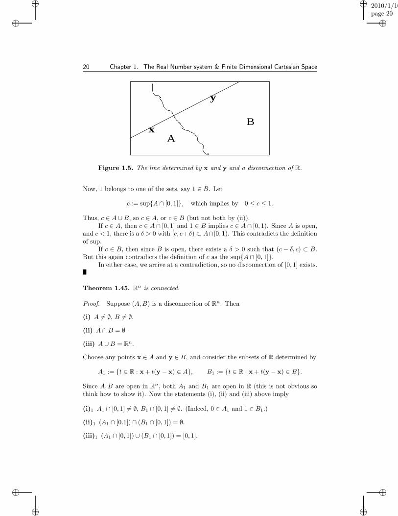
Figure 1.5. The line determined by x and y and a disconnection of R.
Now, 1 belongs to one of the sets, say 1 ∈ B. Let
c := sup{A ∩ [0, 1]}, which implies by 0 ≤ c ≤ 1.
Thus, c ∈ A ∪B, so c ∈ A, or c ∈ B (but not both by (ii)).If c ∈ A, then c ∈ A ∩ [0, 1] and 1 ∈ B implies c ∈ A ∩ [0, 1). Since A is open,
and c < 1, there is a δ > 0 with [c, c+δ) ⊂ A∩ [0, 1). This contradicts the definitionof sup.
If c ∈ B, then since B is open, there exists a δ > 0 such that (c − δ, c) ⊂ B.But this again contradicts the definition of c as the sup{A ∩ [0, 1]}.
In either case, we arrive at a contradiction, so no disconnection of [0, 1] exists.
Theorem 1.45. Rn is connected.
Proof. Suppose (A,B) is a disconnection of Rn. Then
(i) A 6= ∅, B 6= ∅.
(ii) A ∩B = ∅.
(iii) A ∪B = Rn.
Choose any points x ∈ A and y ∈ B, and consider the subsets of R determined by
A1 := {t ∈ R : x + t(y − x) ∈ A}, B1 := {t ∈ R : x + t(y − x) ∈ B}.
Since A,B are open in Rn, both A1 and B1 are open in R (this is not obvious sothink how to show it). Now the statements (i), (ii) and (iii) above imply
(i)1 A1 ∩ [0, 1] 6= ∅, B1 ∩ [0, 1] 6= ∅. (Indeed, 0 ∈ A1 and 1 ∈ B1.)
(ii)1 (A1 ∩ [0.1]) ∩ (B1 ∩ [0, 1]) = ∅.
(iii)1 (A1 ∩ [0, 1]) ∪ (B1 ∩ [0, 1]) = [0, 1].
“muldowney”2010/1/10page 21
i
i
i
i
i
i
i
i
1.3. Topology 21
This means, (A1, B1) is a disconnection of [0, 1] which, we have seen, is con-nected. The contradiction implies that Rn is connected.
Corollary 1.46. The only sets in Rn which are both open and closed are Rn and∅.
Proof. If the nonempty set A 6= Rn is both open and closed, then so is Ac. Then,(A,Ac) would provide a disconnection of Rn.
More restricted notions of connectedness are sometimes used. A set C ispolygonally connected, if for each pair of point x0, xm in C, there is a finite subset{x1, . . . ,xm−1} of C such that the polygon
{xi−1 + t(xi − bfxi−1) : t ∈ [0, 1], i = 1, 2, . . . ,m}
is a subset of C. A set C is arcwise connected if, for each pair of points x,y ∈ C,there is a path joining x to y lying entirely in C. That is, there is a continuousfunction f : [0, 1] 7→ C such that f(0) = x and f(1) = y. Either polygonallyconnected or arcwise connected will imply the set is connected in the sense definedhere. However, the converse is not true. For example, the set {(x, y) ∈ R2 : x 6=0, 0 < y ≤ x2} ∪ {(0, 0)} is connected (in fact, arcwise connected), but is notpolygonally connected. The set {(x, y) ∈ R2 : y = sin( 1
x), x 6= 0} ∪ {(0, y) : −1 ≤y ≤ 1} is connected, but is not arcwise connected.
Exercises
1.33. Property (b) of Proposition 1.31 implies that the intersection of any finitecollection of open sets is open. Show that it is not true that this holds for aninfinite collection of open sets.
1.34. Prove items (a), (b), and (c) of Proposition 1.33.
1.35. Prove that the two definitions of a bounded set are equivalent.
1.36. Prove that the intersection of any finite collection of open sets is open. Hint:Use Property (b) of open sets and induction.
1.37. Prove that {x : |x| ≤ 1} is closed in Rn.
1.38. Prove that a subset U of Rn is open if and only if it is the union of a collectionof open balls.
1.39. If A is a subset of Rn, then A, the closure of A, is the intersection of all closedsets which contain A as a subset. Show that
(a) A is closed.
(b) A ⊂ A.
(c) A = A.
“muldowney”2010/1/10page 22
i
i
i
i
i
i
i
i
22 Chapter 1. The Real Number system & Finite Dimensional Cartesian Space
(d) A ∪B = A ∪B.
(e) ∅ = ∅.(f) Observe that A is the smallest closed set containing A.
(g) Prove that B(O, 1) = {x : |x| ≤ 1}.(h) If A and B are subsets of R, then is A ∩B = A ∩B?
1.40. If A is a subset of Rn, then A◦, the interior of A, is the union of all open setscontained in A. Show that
(a) A◦ is open.
(b) A◦ ⊂ A.
(c) A◦◦ = A◦.
(d) (A ∩B)◦ = A◦ ∩B◦.
(e) Rn◦ = Rn.
(f) Observe that A◦ is the largest open set contained in A.
(g) Prove that B(O, 1)◦
= B(O, 1).
(h) Is there a subset A ⊂ R such that A◦ = ∅ and A = R?
1.41. Let A ⊂ Rn. The derived set A′ of A is the set of all cluster points of A
(a) Prove that A′ is closed.
(b) Prove that A = A ∪A′.
(c) Theorem 1.39 says that A is closed if and only if A′ ⊂ A. A set A forwhich A = A′ is called perfect. Give examples of perfect and non-perfectsets.
1.42. If A ⊂ Rn, then ∂A, the boundary of A, is the set of all points x such thateach neighborhood of x contains a point of A and a point of Ac.
(a) Show A is closed if and only if ∂A ⊂ A.
(b) Show that ∂(∂A) = ∂A; hence ∂A is closed.
(c) Show that ∂A = A\A◦.
1.43. For each of the following sets give its closure, interior, derived set, and bound-ary.
(a) {x ∈ Rn : 0 < |x| < 1}(b) { 1
n ∈ R : n ∈ N}(c) {( 1
n ,1m ) ∈ R2 : n,m ∈ N}
(d) {x ∈ Rn : |x| < 1}.1.44. Without using the Heine-Borel Theorem show that {(x, y) : x2 + y2 < 1} is
not compact on R2.
1.45. Let A and B be open in R. Prove that A×B is open in R2.
1.46. Show that a finite subset of Rn is closed.
“muldowney”2010/1/10page 23
i
i
i
i
i
i
i
i
1.3. Topology 23
1.47. Show that a countable subset of R is not open. Show that it may or may notbe closed.
1.48. Let S be an uncountable subset of R. Show that S has a cluster point.Hint: Show that at least one of the intervals [n, n+ 1], n ∈ Z, must containuncountably many points of S.
1.49. Show that a closed interval is closed.
1.50. Let Q2 denote the set of points in R2 with rational coordinates. What is theinterior of Q2? The boundary of Q2? Show that Q2 is not connected.
1.51. Show that Qc is not connected. Show that (Q2)c is connected, in fact, polyg-onally connected.
1.52. Show that an open connected set in Rn is also polygonally connected.
“muldowney”2010/1/10page 24
i
i
i
i
i
i
i
i
24 Chapter 1. The Real Number system & Finite Dimensional Cartesian Space
“muldowney”2010/1/10page 25
i
i
i
i
i
i
i
i
Chapter 2
Limits, Continuity, andDifferentiation
2.1 Sequences
Definition 2.1. A sequence in Rn is a function from p : N 7→ Rn. Sequences areusually denoted by {pk} where pk := p(k).
Example 2.2 Two simple sequences:
1. pk := 1k , {pk} is a sequence in R.
2. pk := ( 1k , sin(k2)); {pk} is a sequence in R2.
Definition 2.3. A sequence {pk} in Rn is convergent if there exists p ∈ Rn suchthat for each neighborhood U of p, there is a natural number N = N(U) for whichk ≥ N implies pk ∈ U . Write limk→∞ pk = p, or lim{pk} = p.
Equivalently, {pk} converges if there is a point p ∈ Rn such that for eachǫ > 0, there exists and N such that k ≥ N implies
|pk − p| < ǫ.
p is called the limit of the sequence.The sequence {pk} is said to be divergent if it is not convergent.
Proposition 2.4. A convergent sequence cannot have two limits.
Proof. Suppose lim{pk} = p and lim{pk} = q. If ǫ > 0, then
∃N1 such that k ≥ N1 =⇒ |pk − p| < ǫ,
∃N2 such that k ≥ N2 =⇒ |pk − q| < ǫ.
25
“muldowney”2010/1/10page 26
i
i
i
i
i
i
i
i
26 Chapter 2. Limits, Continuity, and Differentiation
If k = max{N1, N2}, then
|q− p| = |q− pk + pk − p| ≤ |pk − q|+ |pk − p| < 2ǫ.
Therefore, |q − p| < 2ǫ for each ǫ > 0; thus |p − q| = 0 (Archimedian Property).Hence, p = q.
Example 2.5 Two simple limits:
1. xk = 1, k = 1, 2, 3, . . ., then limk→∞ xk = 1.
2. limk→∞ 1k = 0 (from the Archimedean Property, Theorem 1.6).
Remarks: Notice that if limk→∞ pk = p, then p is either
(a) a cluster point of the set {pk : k ∈ N}, or
(b) {pk} is ultimately constant and equal to p. (That is, there is an N such thatk ≥ N =⇒ pk = p}.)
Note also that limk→∞ pk = p if and only if limk→∞ |pk − p| = 0.
Theorem 2.6. A convergent sequence is bounded.
Proof. If limk→∞ pk = p, there exists a natural number N such that k ≥ N =⇒|pk − p| < 1. By the triangle inequality
|pk| − |p| ≤ |pk − p| < 1, if k ≥ N=⇒ |pk| < |p|+ 1, if k ≥ N=⇒ |pk| ≤ max{|p1|, . . . , |pN−1|, |p|+ 1}, ∀k ∈ N.
Example 2.7 If pk = k, {pk} is divergent. By the Archimedian property, {pk} isunbounded and so is divergent by Theorem 2.6.
Definition 2.8. If {kj} is a sequence of natural numbers such that k1 < k2 < k3 <. . ., then {pkj
} is called a subsequence of {pk}.
Theorem 2.9. A bounded sequence has a convergent subsequence.
Proof. There are two cases to consider. Either {pk : k ∈ N} is a finite set or itis an infinite set. If it is a finite set, then there is at least one value p such thatpk = p for infinitely many k – these terms in the sequence form a subsequenceof {pk}. In the other case, {pk : k ∈ N} is a bounded infinite set and so by theBolzano-Weierstrass Theorem 1.38, it has a cluster point p. For the ball B(p, 1),there is a k1 such that pk1 ∈ B(p, 1). Suppose kj is such that pkj
∈ B(p, 1j ), then
“muldowney”2010/1/10page 27
i
i
i
i
i
i
i
i
2.1. Sequences 27
there must exist kj+1 > kj such that pkj+1∈ B(p, 1
j+1 ). So, by induction, there
exists a subsequence {pkj} of {pk} such that |pkj
− p| < 1j , j = 1, 2, 3, . . .. The
Archimedian Property implies limj→∞ pkj= p.
Corollary 2.10. If K ⊂ Rn, then K is compact if and only if each sequence ofpoints in K has a subsequence convergent to a point in K.
Proof. “=⇒” The Heine-Borel Theorem shows that K is compact if and only ifit is closed and bounded. Thus, any sequence of points in K is bounded, and soby Theorem 2.9 contains a convergent subsequence. The limit of this sequence iseither a cluster point of the sequence (and hence of K), and so is contained in Ksince K is closed, or else the sequence is ultimately constant so its limit is one ofthe members of the sequence and is in K.
“⇐=” Suppose each sequence in K has a subsequence convergent to a pointof K. To show that K is closed, suppose it is not. Then there exists a cluster pointp of K such that p 6∈ K. Thus, there exists a sequence of points {pk} from K (pkchosen in B(p, 1
k )∩K) such that limk→∞ pk = p 6∈ K, contradicting our hypothesisthat the limit must be in K.
To show that K is bounded, again suppose it is not. Then there exist pk ∈ Ksuch that |pk| > k, k = 1, 2, 3, 4 . . .. Then the unbounded sequence {pk} cannotconverge, contradicting our hypothesis.
Thus, K is closed and bounded, and thus compact, by the Heine-Borel Theo-rem.
Theorem 2.11. A sequence is convergent to a limit p if and only if each subse-quence is convergent and has limit p.
Proof. “=⇒” Suppose limk→∞ pk = p, that is, for each ǫ > 0 there exists N suchthat j ≥ N =⇒ |pj − p| < ǫ. If {pkj
} is a subsequence of {pk}, then
j ≥ N =⇒ kj ≥ j ≥ N =⇒ |pkj− p| < ǫ.
Thus, limj→∞ pkj= p.
“⇐=” Suppose each subsequence {pkj} of {pk} satisfies limj→∞ pkj
= p.But, {pk} is a subsequence of itself.
Example 2.12 If pk = (−1)k, then {pk} is divergent. Indeed,
limk→∞
p2k = 1, limk→∞
p2k+1 = −1.
If {pk} were convergent, these two limits would be the same number by the previoustheorem.
“muldowney”2010/1/10page 28
i
i
i
i
i
i
i
i
28 Chapter 2. Limits, Continuity, and Differentiation
Theorem 2.13. If {pk} and {qk} are sequences in Rn such that
limk→∞
pk = p and limk→∞
qk = q,
then
(i) limk→∞(pk + qk) = p + q,
(ii) limk→∞(pk · qk) = p · q.
Further, if {xk} is a sequence in R such that limk→∞ xk = x, then
(iii) limk→∞ xkpk = xp, and
(iv) limk→∞1xk
pk = 1xp, if xk, x 6= 0.
Proof. Exercise 2
The following result shows that it is sufficient to consider only sequences in R
when considering convergence or divergence.
Theorem 2.14. Let pk = (x1,k, . . . , xn,k) ∈ Rn. Then {pk} is convergent if andonly if each of the sequences {xi,k} is convergent for i = 1, 2, . . . , n. Furthermore,
limk→∞
pk = p = (x1, . . . , xn)⇐⇒ limk→∞
xi,k = xi, i = 1, 2, . . . , n.
Proof. “=⇒” |pk − p| ≥ |xi,k − xi|, for all k ∈ N and for i = 1, 2, . . . , n. Theremainder of the proof is an exercise.
“⇐=” |pk−p| ≤ √nmax{|xi,k−xi| : i = 1, . . . , n}. Thus, if limk→∞ xi,k = xi.i = 1, . . . , n, given any ǫ > 0, there exists Ni such that k ≥ Ni =⇒ |xi,k−xi| < ǫ√
n,
for each i = 1, . . . , n. Let N = max{Ni : i = 1, . . . , n} so k ≥ N implies
|xi,k − xi| <ǫ√n, i = 1, . . . , n =⇒ |pk − p| < ǫ =⇒ lim
k→∞pk = p.
Example 2.15 Further examples of limits of sequences:
(1) limk→∞( 1k ,
1k2 +1) = (0, 1).Use Theorems 2.13 and 2.14 together with limk→∞
1k =
0 (Archimedian Property), to note that limk→∞ 1k2 = 0 and limk→∞ 1
k2 +1 = 1(both by Theorem 2.13), and then Theorem 2.14 to complete the example.
(2) limk→∞2k+3k+2 = 2. Indeed,
2k + 3
k + 2=
2 + 3k
1 + 2k
and limk→∞
1
k= 0 =⇒ lim
k→∞3
k= 0, lim
k→∞2
k= 0,
and the result follows by an application of Theorem 2.13.
“muldowney”2010/1/10page 29
i
i
i
i
i
i
i
i
2.1. Sequences 29
Exercises
2.1. Show that the two definitions of the limit of a sequence are equivalent.
2.2. Prove Theorem 2.13
2.3. Finish the proof of “=⇒” in Theorem 2.14.
2.4. Let xk ≤ zk ≤ yk. Prove that if {xk} and {yk} are convergent with limit c,then {zk} is convergent with limit c.
2.5. Discuss the convergence or divergence of the sequences whose kth terms aregiven by:
(a) kk+1 (b) (−1)kk
k+1 (c) 2k3k2+1
(d) 2k2+33k2+1 (e) ( 1
k , k) (f) ((−1)k, 1k )
2.6. If {xk} is a sequence of nonnegative real numbers which converge to x, show
that limk→∞√xk =
√x. HINT:
√xk −
√x =
xk − x√xk +
√x.
2.7. Let xk =√k + 1−
√k. Discuss the convergence of {xk} and
√k xk.
2.8. Show that a set C in Rn is closed if and only if each convergent sequence inC has its limit in C.
2.9. Show limk→∞ pk = p if and only if limk→∞ |pk − p| = 0.
2.10. If 0 < r < 1, show that limk→∞ rk = 0. HINT: Set r = 11+s , s > 0. Show
that (1 + s)k ≥ 1 + ks, k = 1, 2, . . ., so 0 < rk = 1(1+s)k ≤ 1
1+ns . From this
show that
limk→∞
rk =
{0, if |r| < 1;1, if r = 1
and {rk} is divergent if r = −1 or |r| > 1.
2.11. (Ratio Test) Let {xk} be such that limk→∞∣∣∣xk+1
xk
∣∣∣ = r. Show
(a) If 0 ≤ r < 1, then limk→∞ xk = 0.
(b) If r > 1, then {xk} is divergent.
(c) If r = 1, give examples which show that {xk} may be convergent ordivergent.
HINT: In (a), if r < s < 1, show that for some constant A and all largeenough k, 0 ≤ |xk| ≤ Ask (using the previous exercise).
2.12. Show that the sequence xk
k has limit 0 if −1 ≤ x ≤ 1, and is divergent if|x| > 1.
2.13. Show that limk→∞
xk
k!= 0 for all real numbers x.
2.14. If x > 0 show limk→∞ x1k = 1. HINT: If 0 < x < 1, given ǫ > 0 there exists
N such that k ≥ N implies 11+ǫk < x < 1. (Why?) Therefore
1
(1 + ǫ)k≤ 1
1 + ǫk< x < 1
“muldowney”2010/1/10page 30
i
i
i
i
i
i
i
i
30 Chapter 2. Limits, Continuity, and Differentiation
=⇒ 1
1 + ǫ< x
1k < 1, if k ≥ N
=⇒∣∣∣x
1k − 1
∣∣∣ <ǫ
1 + ǫ< ǫ, if k ≥ N.
Do the case |x| > 1.
2.15. Show limk→∞ k1k = 1. HINT: Let xk = k
1k − 1 > 0. Show k = (1 + xk)
k >k(k+1)
2 x2k, and hence, limk→∞ xk = 0.
2.16. (Root Test) Let {xk} be such that limk→∞
|xk|1k = r. Show
(a) If 0 ≤ r < 1, then limk→∞ xk = 0.
(b) If r > 1, then {xk} is divergent.
(c) If r = 1, then {xk} may be either convergent or divergent.
2.17. If a and b are nonnegative real numbers, show that limk→∞
(ak+bk)1k = max{a, b}.
Definition 2.16. A real sequence {xk} is increasing if x1 ≤ x2 ≤ x3 ≤ . . ., and isdecreasing if x1 ≥ x2 ≥ x3 ≥ . . .. The sequence is monotone if it is either increasingor decreasing.
Theorem 2.17. A monotone sequence is convergent if and only if it is bounded.
Proof. Let {xk} be an increasing sequence. By Theorem 2.6, {xk} convergentimplies {xk} is bounded. On the otherhand, {xk} bounded implies sup{xk : k =1, 2, . . .} = x exists. If ǫ > 0, then x − ǫ is not an upper bound for {xk}, so thereexists an N such that x− ǫ < xN ≤ x. Since {xk} is increasing
k ≥ N =⇒ x− ǫ < xN ≤ xk ≤ x,
that is, k ≥ N =⇒ |xk − x| < ǫ. Thus, the increasing sequence converges to itssupremum.
Remark: Given any ordered field F , each monotone bounded sequence in F isconvergent (with its limit in F if and only if F is complete.
Example 2.18 1. limk→∞ rk = 0 if 0 ≤ r < 1.
Note that 0 < rk+1 = rrk ≤ rk < 1 so {rk} is decreasing and bounded, henceis convergent with 0 ≤ limk→∞ rk < 1. Now {rk+1} is a subsequence of {rk}so they have the same limit. But, limk→∞ rk > 0 implies
limk→∞
rk+1 = r limk→∞
rk < limk→∞
rk,
a contradiction. (A different proof is given in the exercises.)
2. If ak = k2k , then limk→∞ ak = 0. Indeed,
ak+1 =k + 1
2k+1=k + 1
2kak =⇒ 0 < ak+1 ≤ ak.
“muldowney”2010/1/10page 31
i
i
i
i
i
i
i
i
2.1. Sequences 31
Hence, {ak} is convergent and limk→∞ ak ≥ 0. Now,
limk→∞
ak = limk→∞
ak+1 = limk→∞
k + 1
2kak =
1
2limk→∞
ak
implies limk→∞ ak must be zero.
3. For ak = (1 + 1k )k, the sequence {ak} is convergent and 2 ≤ limk→∞ ak ≤ 3.
Indeed, by the binomial theorem
ak = (1 +1
k)k = 1 +
k
k!
1
k+k(k + 1)
2!
1
k2+ . . .+
k!
k!
1
kk
= 1 + 1 +1
2!(1− 1
k) +
1
3!(1− 1
k)(1− 2
k) + . . .+
1
k!(1− 1
k) · · · 2
k
1
k.
Notice that the typical term after the first two has the form
1
ℓ!(1− 1
k) · · · (1− ℓ− 1
k)
and this increases in k. Thus, each term of ak is no greater than the corre-sponding term in ak+1 and ak+1 has one more term. Thus, ak+1 > ak and{ak} is increasing.
We next show ak is bounded. Examining the above, we find
2 < ak ≤ 1 + 1 +1
2!+
1
3!+ . . .+
1
k!
≤ 1 + 1 +1
2+
1
22+ . . .+
1
2k−1≤ 3.
Thus, 2 ≤ limk→∞(1+ 1k )k ≤ 3. This limit is sometimes taken as the definition
of e.
Note: We used the fact that 1 + r + r2 + . . . + rk = 1−rk+1
1−r if r 6= 1. Youwill recall that this is easily proved by denoting the left-hand side by sk andshowing sk − rsk = 1− rk+1.
4. If A > 0, x1 > 0, and xk+1 = 12 (xk+ A
xk), k = 1, 2, . . ., then limk→∞ xk =
√A.
This is an algorithm for computing square roots. Notice that x1 > 0 =⇒ xk >0 by induction. Then
x2k+1 =
1
4(x2k + 2A+
A2
x2k
)
=⇒ x2k+1 −A =
1
4(x2k − 2A+
A2
x2k
) =1
4(xk −
A
xk)2 ≥ 0.
=⇒ x2k+1 ≥ A =⇒ xk+1 ≥
√A, k = 1, 2, . . . .
Hence, xk ≥√A, for k = 2, 3, . . .. Thus,
xk − xk+1 = xk −1
2(xk +
A
xk) =
1
2(xk −
A
xk) =
1
2
x2k −Axk
≥ 0.
“muldowney”2010/1/10page 32
i
i
i
i
i
i
i
i
32 Chapter 2. Limits, Continuity, and Differentiation
So, {xk} is decreasing and bounded below by√A > 0. Therefore, limk→∞ xk =
L ≥√A. But, on the other hand,
xk+1 =1
2(xk +
A
xk) =⇒ L =
1
2(L+
A
L) =⇒ L2 = A =⇒ L =
√A.
The results on monotone sequences are interesting in that, unlike the proceed-ing examples, it is not necessary first to guess the limit of a sequence in order toshow that it converges. Fortunately, we are able to do this in general.
Definition 2.19. A sequence {pk} in Rn is a Cauchy sequence if, for each ǫ > 0,there exists a natural number N = N(ǫ) such that if k,m ≥ N , then
|pk − pm| < ǫ.
Theorem 2.20 (Cauchy Criterion). {pk} is convergent if and only if {pk} is aCauchy sequence.
Proof. “=⇒” Suppose limk→∞ pk = p. Thus, for each ǫ > 0, there exists N suchthat k ≥ N =⇒ |pk − p| < ǫ/2. Hence, if k,m ≥ N , we have
|pk − pm| = |pk − p + p− pm| ≤ |pk − p|+ |p− pm| <ǫ
2+ǫ
2= ǫ.
Thus, {pk} is a Cauchy sequence.“⇐=” We first show that {pk} is bounded and so by the Bolzano-Weierstrass
Theorem (Theorem 1.38) or Theorem 2.9 it has a convergent subsequence. Indeed,choose N so that k,m ≥ N =⇒ |pk − pm| < 1. Then,
k > N =⇒ |pk − pN | < 1 =⇒ |pk| < |pN |+ 1.
Hence, |pk| ≤ max{|p1|, . . . , |pN−1|, |pN |+ 1}.Suppose now that {pkj
} is the subsequence that converges. We claim limj→∞ pkj=
p =⇒ limk→∞ pk = p. Indeed, since limj→∞ pkj= p, for each ǫ > 0 there is a N1
such that j ≥ N1 =⇒ |pkj− p| < ǫ/2. Since {pk} is a Cauchy sequence, there is
also an N2 such that m, k ≥ N2 =⇒ |pk −pm| < ǫ/2. Take any kj ≥ max{N1, N2}.Then for k ≥ max{N1, N2}, we have
|pk − p| = |pk − pkj+ pkj
− p| ≤ |pk − pkj|+ |pkj
− p| < ǫ
2+ǫ
2= ǫ.
Thus, limk→∞ pk = p.
Remark: An ordered field F is complete if and only if each Cauchy sequence in Fis convergent (with its limit in F ).
“muldowney”2010/1/10page 33
i
i
i
i
i
i
i
i
2.1. Sequences 33
Example 2.21 1. The sequence {(−1)k} is divergent.
In fact, we have for xk = (−1)k that |xk − xk+1| = 2 for all k, and so {xk}cannot be a Cauchy sequence.
2. For xk = 1 + 12 + 1
3 + . . .+ 1k , {xk} is divergent. Indeed,
|x2k − xk| =1
k + 1+
1
k + 2+ . . .+
1
2k≥ 1
2k+ . . .+
1
2k︸ ︷︷ ︸k times
=1
2.
Therefore, |x2k − xk| ≥ 12 for all k and {xk} cannot be a Cauchy sequence.
Exercises
2.17. Show that the following sequences are divergent by proving directly they arenot Cauchy sequences.(a) {k} (b) {(−1)k(1− 1
k )}2.18. Show directly that the following are Cauchy sequences and hence are conver-
gent.(a) {k+1
k } (b) {1 + 11! + 1
2! + . . .+ 1k!}.
2.19. Determine whether each of the following sequences is convergent or divergent.In the case of convergence, find the limit.
(a){
4k2+k+4(1+k)(2+ 3
k
}(b)
{k3+k2+1(k+1)4
}
(c){
(k2+1)2
(k+1)(k+2)(k+3)
}(d) {k2 + k}
(e) {1− k3} (f)
{sin(
kπ3
)+3k
k
}
(g)
{sin(
kπ3
)+2k2
k
}(h)
{k2+1k3+1 cos2
(kπ4
)}
(i){k3 − [k3 ]
},
where [x] denotes the greatest integer not exceeding x.
2.20. For what values of x are the following convergent, divergent? Wherever youcan, give the limit.
(a){
xk
(k+2)(k+1)
}(b)
{(k + 1)(k + 2)xk
}
(c){
xk+kxk+1+(k+1)
}(d)
{kxk+xk−1+1kxk−1+1
}
(e){xk
k!
}(f)
{k!xk
}
2.21. If a1 = 2, ak+1 =√
6 + ak, k ≥ 1, show that {ak} is increasing andlimk→∞ ak = 3.
“muldowney”2010/1/10page 34
i
i
i
i
i
i
i
i
34 Chapter 2. Limits, Continuity, and Differentiation
2.22. Show that the sequence 1, 1.4, . . . , ak, . . ., in which (2ak+3)∗ak+1 = 4+3ak,is monotone and that limk→∞ ak =
√2.
2.23. If a1 = 1 and ak+1(1 + ak) = 12, show that limk→∞ ak = 3. Hint: Showa2k+1 is increasing and a2k is decreasing.
2.24. Show the following
(a) If limk→∞ ak = 0, then limk→∞ σk = 0, where σk = a1+...+ak
k .
(b) If limk→∞ ak = a, then limk→∞ σk = a. Hint: limk→∞(ak − a) = 0.
(c) Give an example to show that {σk} may be convergent even though {ak}is not.
2.25. We have seen that limk→∞ x1k = 1 if x > 0. (Exercise 15). An easier proof is
now available to us from our results on monotone sequences. Show {x 1k } is
monotone and bounded, hence convergent. Consider the subsequence {x 12k }
and deduce the result.
2.26. Let {xk} be a sequence of positive real numbers. Show that
limk→∞
xk+1
xk= r =⇒ lim
k→∞x
1k
k = r.
Hint: If r > 0 and ǫ > 0, then there exist positive numbers A,B and a naturalnumber N such that
A(r − ǫ)k ≤ xk ≤ B(r + ǫ)k, ∀ k > N.
2.27. By applying the last exercise to the sequence {kk
k! } show that
limk→∞
k
(k!)1k
= e, where e = limk→∞
(1 +1
k)k.
2.28. Let sk = (1 + 1k )k, tk = 1 + 1
1! + 12! + . . . + 1
k! . We have seen that bothsequences are convergent. Show that they have the same limit. Hint: Firstuse the Binomial Theorem to show
sk = 1 +1
1!+
1
2!(1 − 1
k) + . . .+
1
k!(1 − 1
k) · · · (1− k − 1
k) ≤ tk.
Next, with m fixed, and k ≥ m, show that
sk ≥ 1 +1
1!+
1
2!(1− 1
k) + . . .+
1
m!(1− 1
k) · · · (1− m− 1
k)
and deduce that limk→∞ sk ≥ tm for each m.
2.29. Show that every sequence of real numbers has a monotone subsequence. (Becareful.)
2.30. Let f be an ordered field. Show that the following statements are equivalent.
(a) F is complete (sets bounded above have a supremum in F ).
(b) F has the nested interval property.
“muldowney”2010/1/10page 35
i
i
i
i
i
i
i
i
2.2. Continuity 35
(c) Each bounded monotone sequence in F converges to an element of F .
(d) Each Cauchy sequence in F converges to an element of F .
Discussion: All four statements in this problem are equivalent. However, (a),(b), (c) are inapplicable if one wishes to consider completeness for sets whichare not ordered, whereas (d) is applicable to any set X for which distancebetween points, i.e., a metric, has been defined. A function ρ : X ×X 7→ R
is a metric if
(i) ρ(x, y) ≥ 0, ∀ x, y ∈ X.(ii) ρ(x, y) = 0⇐⇒ x = y.
(iii) ρ(x, y) = ρ(y, x), ∀ x, y ∈ X .
(iv) ρ(x, y) ≤ ρ(x, z) + ρ(z, y) for all x, y, x ∈ X . (Triangle inequality)
The pair (X, ρ) is called a metric space. A sequence {xk} in X is a Cauchysequence (or fundamental sequence) if, for each ǫ > 0, there exists a naturalnumber N such that m, k ≥ N =⇒ ρ(xm, xk) < ǫ. A metric space {X, ρ} iscalled complete if each Cauchy sequence in {X, ρ} is convergent (i.e., thereexists x ∈ X such that limk→∞ ρ(xk, x) = 0 whenever {xk} is a Cauchysequence). For example, the space {Rn, ρ} is a complete metric space ifρ(p,q) = |p − q|. It is easily seen that ρ is a metric from the properties(i),(ii),(iii),and (iv) above. Theorem 2.20 implies the completeness of Rn.
2.2 Continuity
Let f : Rn 7→ Rm, and let D ⊂ Rn be the domain of f .
Definition 2.22. Suppose p0 ∈ D, we say f is continuous at p0 if, for eachneighborhood V of f(p0), there exist a neighborhood U of p0 such that p ∈ U∩D =⇒f(p) ∈ V , (i.e. f(U) ⊂ V ). Equivalently, f is continuous at p0 if, for each ǫ > 0,there is a δ > 0 such that
p ∈ D and |p− p0| < δ =⇒ |f(p)− f(p0)| < ǫ.
In general, δ = δ(ǫ,p0).
Definition 2.23. The function f is continuous on D if it is continuous at eachpoint p0 of D.
Example 2.24 Let f(x) = x2, −1 ≤ x ≤ 1, then D = [−1, 1], f(D) = [0, 1], and
|f(x)− f(x0)| = |x2 − x20| = |(x− x0)(x + x0)| ≤ |x− x0|(|x| + |x0|)
=⇒ |f(x)− f(x0)| ≤ 2|x− x0| for x, x0 ∈ [−1, 1]
If ǫ > 0, take δ = ǫ/2, then |x− x0| < δ and x, x0 ∈ [−1, 1] implies
|f(x)− f(x0)| < ǫ,
so f is continuous on [−1, 1].
“muldowney”2010/1/10page 36
i
i
i
i
i
i
i
i
36 Chapter 2. Limits, Continuity, and Differentiation
������������������
f
D
f(D)
p0
pU V
f(p )0
Rn
R m
f(p).. .
.
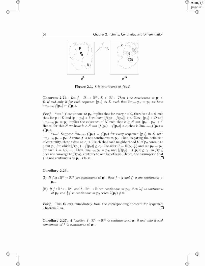
Figure 2.1. f is continuous at f(p0).
Theorem 2.25. Let f : D 7→ Rm, D ⊂ Rn. Then f is continuous at p0 ∈D if and only if for each sequence {pk} in D such that limk∞ pk = p0 we havelimk→∞ f(pk) = f(p0).
Proof. “=⇒” f continuous at p0 implies that for every ǫ > 0, there is a δ > 0 suchthat for p ∈ D and |p − p0| < δ we have |f(p) − f(p0)| < ǫ. Now, {pk} ∈ D andlimk→∞ pk = p0 implies the existence of N such that k ≥ N =⇒ |pk − p0| < δ.Hence, for this N we have k ≥ N =⇒ |f(pk)− f(p0)| < ǫ; that is limk→∞ f(pk) =f(p0).
“⇐=” Suppose limk→∞ f(pk) = f(p0) for every sequence {pk} in D withlimk→∞ pk = p0. Assume f is not continuous at p0. Then, negating the definitionof continuity, there exists an ǫ0 > 0 such that each neighborhood U of p0 contains apoint pU for which |f(pU )− f(p0)| ≥ ǫ0. Consider U = B(p0,
1k ) and set pU = pk,
for each k = 1, 2, . . .. Then limk→∞ pk = p0, and |f(pk) − f(p0)| ≥ ǫ0, so f(pk)does not converge to f(p0), contrary to our hypothesis. Hence, the assumption thatf is not continuous at p0 is false.
Corollary 2.26.
(i) If f, g : Rn 7→ Rm are continuous at p0, then f + g and f · g are continuous atp0.
(ii) If f : Rn 7→ Rm and λ : Rn 7→ R are continuous at p0, then λf is continuousat p0 and 1
λf is continuous at p0 when λ(p0) 6= 0.
Proof. This follows immediately from the corresponding theorem for sequencesTheorem 2.13.
Corollary 2.27. A function f : Rn 7→ Rm is continuous at p0 if and only if eachcomponent of f is continuous at p0.
“muldowney”2010/1/10page 37
i
i
i
i
i
i
i
i
2.2. Continuity 37
Proof. If f(p) = (f1(p), . . . , fm(p)) and limk→∞ pk = p0, then
limk→∞
f(pk) = f(p0)⇐⇒ limk→∞
fi(pk) = fi(p0), i = 1, 2, . . . ,m,
by Theorem 2.14.
Example 2.28 Some examples of continuous and discontinuous functions:
(1) D = [0, 1], f(x) = 1, for 0 < x ≤ 1, and f(0) = 0. Then f is discontinuousat x = 0. Indeed, if xk is any sequence in (0, 1] with limk→∞ xk = 0, thenf(xk) = 1 so limk→∞ xk = 1 6= 0.
(2) Let D = R, f(x) = sin( 1x ), for x 6= 0 and f(0) = 0. Then f is discontinuous at
x = 0 since
limk→∞
2
(2k + 1)π= 0 and
{f( 2
(2k + 1)π
)}={(−1)k+1
},
and the latter sequence is not convergent.
Remark: The discontinuity in the first example is removable, i.e. the dis-continuity at x = 0 can be removed by changing the value of the functionat 0. The discontinuity in the second example is essential since no matterwhat value is assigned to the function at x = 0, the discontinuity cannot beremoved.
(3) D = R2, f(x, y) = xyx2+y2 , for (x, y) 6= O and f(0, 0) = 0. The function f is
discontinuous at (0, 0). Indeed, for the sequence of points
pk = (1
k,1
k), k ∈ N, lim
k→∞pk = O and lim
k→∞f(pk) =
1
k2/(2
1
k2) =
1
26= 0.
The discontinuity at (0, 0) is essential since if qk = ( 1k ,
12k ), then
limk→∞
qk = O, but limk→∞
f(qk) =1
2k2/(
1
k2+
1
4k2) =
2
5.
So we obtain two different limits from two different choices of sequences.
(4) D = R2, f(x, y) = x2y2
x2+y2 , for (x, y) 6= O, and f(0, 0) = 0. This function f is
continuous on R2.
We first show continuity at p0 = (x0, y0) 6= O. If limk→∞(xk, yk) = (x0, y0),then limk→∞ x2
ky2k = x2
0y20 , and limk→∞(x2
k + y2k) = x2
0 + y20 6= 0. So, by
Theorem 2.13, limp→p0f(p) = f(p0).
When p0 = O, we have x20 + y2
0 = 0, so because the denominator becomeszero, we must prove it directly: if (x, y) 6= (0, 0), the x2 + y2 6= 0 and
|f(x, y)− f(0, 0)| = x2y2
x2 + y2≤ x4 + 2x2y2 + y4
2(x2 + y2)=x2 + y2
2=
1
2|(x, y)|2.
Hence, if |(x, y)| = |(x, y)− (0, 0)| <√
2ǫ, we have |f(x, y)− f(0, 0)| < ǫ.
“muldowney”2010/1/10page 38
i
i
i
i
i
i
i
i
38 Chapter 2. Limits, Continuity, and Differentiation
Recall that if f : Rn 7→ Rℓ and g : Rℓ 7→ Rm, then g ◦ f is defined asg ◦ f(p) = g(f(p)). The domain of g ◦ f is {p ∈ Df : f(p) ∈ Dg} = f−1(Dg) ⊂ Df .
Theorem 2.29. Suppose p0 ∈ Dg◦f . Then g ◦ f is continuous at p0 if
(i) f is continuous at p0, and
(ii) g is continuous at f(p0).
Proof. If {pk} is a sequence in Dg◦f ⊂ Df such that limk→∞ pk = p0, then{f(pk)} is a sequence in Dg such that limk→∞ f(pk) = f(p0), since f is continuousat p0. Since g is continuous at f(p0), we then have limk→∞ g(f(pk)) = g(f(p0)).Thus, limk→∞ g ◦ f(pk) = g ◦ f(p0). Thus, by Theorem 2.25, g ◦ f is continuous atp0.
Corollary 2.30. If f : Rn 7→ Rm is continuous at p0, then |f | : Rn 7→ R iscontinuous at p0.
Proof. If g(q) = |q| for q ∈ Rm, then g is continuous on Rm since
||q| − |q0|| ≤ |q− q0|.
Thus, if ǫ > 0 is given, |q − q0| < ǫ =⇒ ||q| − |q0|| < ǫ. Therefore, g ◦ f = |f | iscontinuous at p0 since g is continuous at f(p0).
2.3 Global Properties of Continuous Functions
Again recall the notation that if f : Rn 7→ Rm with domain D ⊂ Rn and rangef(D) ⊂ Rm, then for A ⊂ Rn, f(A) := {f(p) : p ∈ A ∩ D}, and for B ⊂ Rm,f−1(B) := {p : f(p) ∈ B}.
Example 2.31 Some functions and inverse images of part of their range:
(1) f(x) = x2, −1 ≤ x ≤ 1. Then
f([0,1
2]) = [0,
1
4], f([
1
2, 2]) = [
1
4, 1], f−1([
1
4, 3]) = [−1.− 1
2] ∪ [
1
2, 1].
(2) f(x) = sin(x), −∞ < x <∞. Then
f−1([0, 1)) = ∪∞k=−∞
([2kπ, (2k + 1)π]\{(4k + 1)π/2}
).
“muldowney”2010/1/10page 39
i
i
i
i
i
i
i
i
2.3. Global Properties of Continuous Functions 39
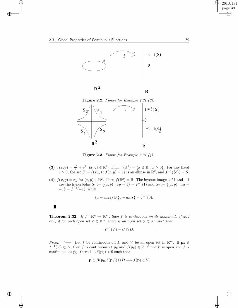
f c= f(S)
0
RR 2
S
Figure 2.2. Figure for Example 2.31 (3).
R 2
fS2
S1
0
R
2
S1
S2
1 = f ( S
−1 = f(S )
1)
Figure 2.3. Figure for Example 2.31 (4).
(3) f(x, y) = x2
4 + y2, (x, y) ∈ R2. Then f(R2) = {x ∈ R : x ≥ 0}. For any fixedc > 0, the set S := {(x, y) : f(x, y) = c} is an ellipse in R2, and f−1({c}) = S.
(4) f(x, y) = xy for (x, y) ∈ R2. Then f(R2) = R. The inverse images of 1 and −1are the hyperbolas S1 := {(x, y) : xy = 1} = f−1(1) and S2 := {(x, y) : xy =−1} = f−1(−1), while
{x− axis} ∪ {y − axis} = f−1(0).
Theorem 2.32. If f : Rn 7→ Rm, then f is continuous on its domain D if andonly if for each open set V ⊂ Rm, there is an open set U ⊂ Rn such that
f−1(V ) = U ∩D.
Proof. “=⇒” Let f be continuous on D and V be an open set in Rm. If p0 ∈f−1(V ) ⊂ D, then f is continuous at p0 and f(p0) ∈ V . Since V is open and f iscontinuous at p0, there is a δ(p0) > 0 such that
p ∈ B(p0, δ(p0)) ∩D =⇒ f(p) ∈ V,
“muldowney”2010/1/10page 40
i
i
i
i
i
i
i
i
40 Chapter 2. Limits, Continuity, and Differentiation
which impliesB(p0, δ(p0)) ∩D ⊂ f−1(V ), ∀ p0 ∈ f−1(V ). (2.1)
Hence, if we setU := ∪p0∈f−1(V )B(p0, δ(p0)),
then U is open and (2.1) implies
U ∩D ⊂ f−1(V ). (2.2)
However, from the definition of U , p0 ∈ f−1(V ) implies p0 ∈ U ∩D, i.e.
f−1(V ) ⊂ U ∩D. (2.3)
So, U is an open subset of Rn and, from (2.2) and (2.3),
U ∩D = f−1(V ).
“⇐=” Suppose that for each open V ⊂ Rm, there exists an open U ⊂ Rn suchthat
U ∩D = f−1(V ).
Let p0 ∈ D, and ǫ > 0 be given. Consider V = B(f(p0), ǫ). Then there exists anopen U ⊂ Rn with U ∩D = f−1(V ). In particular, p0 ∈ U , so U is a neighborhoodof p0, and
p ∈ U ∩ V =⇒ f(p) ∈ V.Thus, f is continuous at p0
Theorem 2.33 (Preservation of Connectedness). Suppose f : Rn 7→ Rm. Iff is continuous on D and D is connected, then f(D) is connected.
Proof. Suppose f(D) is not connected. Then there exist open sets V1 and V2 inRm such that
(i) V1 ∩ f(D) 6= ∅ and V2 ∩ f(D) 6= ∅;
(ii) (V1 ∩ f(D)) ∩ (V2 ∩ f(D)) = ∅; and
(iii) (V1 ∩ f(D)) ∪ (V2 ∩ f(D)) = f(D).
By the Global Continuity Theorem (Theorem 2.32), there exist open sets U1
and U2 in Rn such that
U1 ∩D = f−1(V1), U2 ∩D = f−1(V2).
Then
(i)’ U1 ∩D 6= ∅, U2 ∩D 6= ∅, from (i),
(ii)’ (U1 ∩D) ∩ (U2 ∩D) = ∅, from (ii),
“muldowney”2010/1/10page 41
i
i
i
i
i
i
i
i
2.3. Global Properties of Continuous Functions 41
(iii)’ (U1 ∩D) ∪ (U2 ∩D) = D, from (iii)
Thus, D is disconnected, a contradiction to our hypothesis that D is connected.Therefore, our assumption that f(D) is disconnected is false.
Corollary 2.34. Suppose f : Rn 7→ R. Let D be a connected subset of Rn, and fbe a continuous real-valued function on D. If p,q ∈ D and f(p) < k < f(q), thenthere is a p0 ∈ D such that f(p0) = k.
Proof. If there is no such p0, then the sets V1 = (−∞, k) and V2 = (k,+∞) providea disconnection of f(D) ; a contradiction to Theorem 2.33.
Example 2.35 At any time there are two antipodal points on the equator at thesame temperature. Indeed, let T (x) be temperature. Then T (x + 2π) = T (x).We suppose T is continuous and consider f(x) = T (x + π) − T (x). Then f(0) =T (π) − T (0), while f(π) = T (2π) − T (π) = T (0) − T (π) = −f(0). If f(0) = 0,then T (π) = T (0); otherwise, f(0) and f(π) are of opposite sign and k = 0 is avalue between them. In the latter case, by Corollary 2.34, there is a point x0, withf(x0) = 0 = T (x0 + π)− T (x0); i.e. T (x0 + π) = T (x0).
Theorem 2.36 (Preservation of Compactness). Let f : Rn 7→ Rm. If D iscompact and f is continuous on D, then f(D) is compact.
Proof. Let G be an open covering of f(D). For each V ∈ G there is an open setU ⊂ Rn such that
U ∩D = f−1(V ) by Theorem 2.32. (2.4)
Since {V : V ∈ G} covers f(D), the collection {U : U ∩D = f−1(V ), V ∈ G} coversD. Since D is a compact set, there must be a finite subcover {U1, . . . , Uk}. From(2.4), the V ’s corresponding to the Ui satisfy f(Ui) ⊂ Vi so {V1, . . . , Vk} coversf(D). Thus, the cover G contains a finite subcover of f(D). Since we began withan arbitrary cover of f(D), so f(D) must be compact.
Corollary 2.37. A continuous function on a compact set is bounded.
Proof. f(D) is compact and therefore closed and bounded by the Heine-BorelTheorem.
Corollary 2.38. A continuous real-valued function f : D ⊂ Rn 7→ R on a com-pact set D achieves its supremum and infimum, that is, it has a maximum and aminimum value.
Proof. Let f : D ⊂ Rn 7→ R be continuous. Then f(D) is a compact subset of R
(Theorem 2.36). Let M := sup{f(p) : p ∈ D} = sup f(D). We wish to show that
“muldowney”2010/1/10page 42
i
i
i
i
i
i
i
i
42 Chapter 2. Limits, Continuity, and Differentiation
M ∈ f(D), that is, that M = f(p0) for some p0 ∈ D. Suppose M 6∈ f(D), whichimplies M > f(p) for all p ∈ D. Consider the function
g(p) =1
M − f(p)> 0, for p ∈ D.
Then g is continuous on D. (Why?) Since D is compact, g is bounded by Corollary2.37. Hence, there exists a finite number A such that
0 < g(p) ≤ A, ∀ p ∈ D
=⇒ 0 <1
M − f(p)≤ A, ∀ p ∈ D
=⇒ 1
A≤M − f(p), ∀ p ∈ D
=⇒ f(p) ≤M − 1
A< M, ∀ p ∈ D.
The last inequality contradicts the fact that M is the least upper bound of f(D).Hence, we must have M ∈ f(D).
Exercises
2.32. Prove that the two definitions of continuity are equivalent.
2.33. Let f(x) =√x, x ≥ 0. Show that f is continuous on [0,∞).
2.34. Show that every real polynomial of odd degree has at least one real root.
2.35. Show that x4 + 7x3 − 9 has at least two real roots.
2.36. Suppose f and g are continuous real valued functions on [0, 1] such thatf(0) < g(0) and f(1) > g(1). Prove that there exists x ∈ (0, 1) such thatf(x) = g(x). Hint: Draw a picture.
2.37. Give an alternative proof of Theorem 2.36 by showing directly that f(D) isclosed and bounded if f is continuous on D and D is closed and bounded.Hint: If f(D) is not bounded, then there exists pk ∈ D such that |f(pk)| > k,k = 1, 2, . . .. If f(D) is not closed, there is at least one cluster point q off(D) with q 6∈ f(D). The latter means there are points pk ∈ D so thatlimk→∞ f(pk) = limk→∞ qk = q 6∈ f(D). Show that each case leads to acontradiction of the hypothesis.
2.38. Show that f(x) = 1x is not uniformly continuous on (0, 1].
2.4 Uniform Continuity
Definition 2.39. A function f : D ⊂ Rn 7→ Rm is uniformly continuous on D if,for each ǫ > 0, there is a δ > 0 so that
(p,q ∈ D and |p− q| < δ) =⇒ |f(p)− f(q)| < ǫ.
“muldowney”2010/1/10page 43
i
i
i
i
i
i
i
i
2.4. Uniform Continuity 43
Here the δ depends only on ǫ (and possibly D), but not on the choice of points.
Example 2.40 Some examples on uniform continuity:
(1) f(x) = x, −∞ < x < +∞ (D = R), is uniformly continuous on R. Obviously,if x, y ∈ R and |x− y| < ǫ, then |f(x)− f(y)| < ǫ.
(2) f(x) = x2, 0 ≤ x ≤ 1 (D = [0, 1]), is uniformly continuous on D. Indeed,
|f(x)− f(y)| = |x2 − y2| = |x− y||x+ y| ≤ 2|x− y| for x, y ∈ [0, 1].
Thus, if x, y ∈ D and |x − y| < ǫ2 , then |f(x) − f(y)| < ǫ, so f is uniformly
continuous on D = [0, 1].
(3) f(x) = x2, 0 ≤ x < +∞ (D = [0,+∞)), then f is not uniformly continuous onD. We will show the condition is not satisfied for ǫ = 1 by any choice of δ.Let δ > 0 be given and choose x = 1
δ , y = 1δ + δ
2 . Then
|x− y| = δ
2< δ and |f(x)− f(y)| = |x− y||x+ y| = δ
2(2
δ+δ
2) > 1.
Thus, f is not uniformly continuous on [0,∞).
(4) f(x) =√x, 1 ≤ x < +∞ (D = [1,+∞)). Then f is uniformly continuous on
D. Indeed,
|f(x)− f(y)| = |√x−√y| = |x− y|√x+√y≤ 1
2|x− y|, ∀ x, y ∈ [1,+∞).
Thus, if |x− y| < 2ǫ and x, y ∈ [0,+∞), we have |f(x)− f(y)| < ǫ.
(5) f(x) =√x, D = [0,+∞), is uniformly continuous on D. We again use
|f(x)− f(y)| = |x− y|√x+√y.
We may assume that x > y and suppose |x − y| < δ. If x ≥ δ, then |f(x) −f(y)| < δ√
δ=√δ. If y < x < δ, then |f(x)−f(y)| = √x−√y <
√δ−0 =
√δ.
In either case, we see that(|x− y| < δ = ǫ2 and x, y ∈ [0,+∞)
)=⇒ |f(x) − f(y)| < ǫ.
Theorem 2.41. Let f : D ⊂ Rn 7→ Rm. If f is continuous on D and D is compact,then f is uniformly continuous on D.
Proof. Let ǫ > 0 be given. By the continuity of f on D, for each p0 ∈ D, thereexists a δ(ǫ,p0) > 0 such that
p ∈ B(p0, δ(ǫ.p0)) ∩D =⇒ |f(p)− f(p0| <ǫ
2.
“muldowney”2010/1/10page 44
i
i
i
i
i
i
i
i
44 Chapter 2. Limits, Continuity, and Differentiation
Now, G := {B(p0, δ(ǫ.p0)/2) : p0 ∈ D} forms an open cover of D. Since D iscompact, there are p1, . . . ,pk in D such that the corresponding balls form a finitesubcover of D:
D ⊂ ∪kj=1B(pj , δ(ǫ.pj)/2). (2.5)
Let δ(ǫ) = min{δ(ǫ.pj)/2 : j = 1, . . . , k}. If p,q ∈ D and |p − q| < δ(ǫ), thenp ∈ B(pj , δ(ǫ.pj)/2) for some j by (2.5). Thus,
|p− pj | <1
2δ(ǫ.pj). (2.6)
But, |p− q| < δ(ǫ) < 12δ(ǫ.pj), and hence from (2.6)
|q− pj | ≤ |q− p|+ |p− pj | ≤ δ(ǫ.pj). (2.7)
Therefore,
(2.6) =⇒ |f(p)− f(pj)| <ǫ
2and (2.7) =⇒ |f(q)− f(pj)| <
ǫ
2.
Therefore, from the triangle inequality, if p,q ∈ D and |p−q| < δ(ǫ), then |f(p)−f(q)| < ǫ. So, f is uniformly continuous on D.
Alternative Proof: Suppose f is not uniformly continuous on D. Negatingthe definition of uniform continuity, there exists and ǫ0 > 0, such that for everyδ > 0, there exists p,q ∈ D with |p− q| < δ but |f(p)− f(q)| ≥ ǫ0. In particular,there exist pk,qk such that |pk − qk| < 1
k and |f(pk)− f(qk)| ≥ ǫ0 > 0.Now {pk} ⊂ D and D is compact, hence bounded. Therefore, there is a
subsequence {pkj} converging to some point p0 in D; limj→∞ pkj
= p0 (Corollary2.10). Now
|qkj− p0| ≤ |qkj
− pkj|+ |qkj
− p0| ≤1
kj+ |qkj
− p0|,
and the right hand side tends to zero as j → ∞. Hence, limj→∞ qkj= p0 also.
But, the continuity of f at any point p0 ∈ D implies that
limj→∞
(f(pkj)− f(qkj
)) = f(p0)− f(p0) = 0,
contradicting |f(pk)− f(qk)| ≥ ǫ0 > 0 for all k.
Exercises
2.38. If f(x) = 1x , x 6= 0, then f is continuous on its domain.
2.39. Show that a polynomial
f(x) = anxn + an−1x
n−1 + . . .+ a1x+ a0, (ai constants)
is continuous on R. Hint: Show that f(x) = constant and g(x) = x arecontinuous on R, and deduce the general result from Corollary 2.26.
“muldowney”2010/1/10page 45
i
i
i
i
i
i
i
i
2.4. Uniform Continuity 45
2.40. Let f : R 7→ R be defined by
f(x) =
{1− x, x ∈ Q;x, x 6∈ Q.
Show that f is continuous at x = 12 and discontinuous elsewhere.
2.41. Let f : R 7→ R be continuous on R. Show that if f(x) = 0 for all x ∈ Q, thenf(x) = 0 for all x ∈ R.
2.42. Use the inequalities | sin(x)| ≤ |x| and | cos(x)| ≤ 1 and the formula
sin(x)− sin(u) = 2 sin(x− u
2) cos(
x + u
2)
to show that the sine function is uniformly continuous on R.
2.43. Using the results of exercises 38 and 42 show that the function defined by
g(x) =
{x sin( 1
x ), x 6= 0;0, x = 0;
is continuous on R.
2.44. Is it possible for f and g to be discontinuous and yet g ◦ f be continuous?
2.45. Let f be continuous on D.
(a) Is it true that D open implies f(D) open? (This one is easy.)
(b) Is it true thatD closed implies f(D) closed? Hint: Consider f(x) = 11+x2
on R.
2.46. If f(x) = 11+x2 , then f is uniformly continuous on R.
2.47. Let f be a real-valued function with domain D, D being an open subset ofRn. Prove that f is continuous if and only if the sets
{p : f(p) > α}, {p : f(p) < α}
are open for each α ∈ R.
2.48. If f(x, y) = xy + x4 − y4, then the equation f(x, y) = 0 has at least foursolutions on any circle x2 + y2 = R2 > 0.
2.49. Prove the following facts about uniformly continuous functions:
(a) Let f be uniformly continuous on (0, 1] and {xk} be a sequence ofreal numbers such that 0 < xk ≤ 1 and limk→∞ xk = 0. Prove thatlimk→∞ f(xk) exists. Hint: What was Cauchy’s name?
(b) If f is uniformly continuous on (0, 1], then f may be defined at x = 0 sothat f is continuous on [0, 1].
(c) If f : Rn 7→ Rm, and f is uniformly continuous on the domain D ⊂ Rn,then f may also be defined on D\D so that f is continuous on D. (Ddenotes the closure of D.)
See Exercise 1.39 and 1.41.
“muldowney”2010/1/10page 46
i
i
i
i
i
i
i
i
46 Chapter 2. Limits, Continuity, and Differentiation
2.50. If f : Rn 7→ Rm with domain D ⊂ Rn, the set
G := {(p, f(p)) : p ∈ D} ⊂ Rn+m
is called the graph of f . Suppose D is connected. Is it true that f is contin-uous on D if and only if G is connected? What if “connected” is replaced by“closed”? “Compact”? Prove any statements you believe to be true and finda counterexample for any false statements.
2.51. If f is real valued and f is continuous at p0 with f(p0) > 0, then f(p) > 0for each p in a neighborhood of p0. Hint: ǫ = 1
2f(p0).
2.52. Prove that f is continuous at a point p0 in its domain D if and only if,for each sequence {pk} of points in D such that limk→∞ pk = p0, we have{f(pk)} convergent. (We say nothing about limk→∞ f(pk).)
2.5 Limits
The notion of a limit which was introduced for sequence can, as you recall from firstyear Calculus, be extended to any function.
Definition 2.42. Let f : Rn 7→ Rm with domain D ⊂ Rn. Let p0 be a clusterpoint of D (it is not assumed that p0 ∈ D). A point L ∈ Rm is the limit at p0 of fif, for each ǫ > 0, there exists a δ > 0 such that
(p ∈ D and 0 < |p− p0| < δ) =⇒ |f(p)− L| < ǫ.
Writelim
p→p0
f(p) = L.
If no such L exists, we say the limit at p0 of f does not exist.
Example 2.43 (1) f(x, y) =xy√x2 + y2
is defined for (x, y) 6= O, i.e. D =
R2\{O}. We claim lim(x,y)→(0,0) f(x, y) = 0. Indeed, using (a + b)2 ≥ 0 =⇒a2 + b2 ≥ 2ab, we see that
∣∣∣∣∣xy√x2 + y2
∣∣∣∣∣ ≤1
2
x2 + y2
√x2 + y2
=1
2
√x2 + y2 =
1
2|(x, y) − (0, 0)|.
If ǫ > 0 is given, then 0 < |(x, y)| < 2ǫ implies |f(x, y)| < ǫ.
(2) The function defined on R2 by
f(x, y) =
{0, if y 6= x2;1, if y = x2;
does not have a limit at O = (0, 0) since each neighborhood of (0, 0) containspoints (x, y) 6= (0, 0) at which f(x, y) = 0 and at which f(x, y) = 1.
“muldowney”2010/1/10page 47
i
i
i
i
i
i
i
i
2.5. Limits 47
Just as in the case of sequences there is a Cauchy criterion for the existenceof limp→p0
f(p).
Theorem 2.44 (Cauchy Criterion). The limit limp→p0f(p) exists if and only
if for each ǫ > 0, there is a δ > 0 such that
p,q ∈ D ∩(B(p0, δ)\{p0}
)=⇒ |f(p)− f(q)| < ǫ.
Proof. “=⇒” Suppose limp→p0f(p) = L; thus, if ǫ > 0 is given, there exists a
δ > 0 such that
p ∈ D, 0 < |p− p0| < δ =⇒ |f(p)− L| < ǫ/2.
Then, if p,q ∈ D ∩(B(p0, δ)\{p0}
), we have
|f(p)− f(q)| ≤ |f(p)− L|+ |f(q)− L| < ǫ/2 + ǫ/2 = ǫ,
so Cauchy’s Criterion is satisfied.“⇐=” Let Cauchy’s Criterion be satisfied, that is, for a given ǫ > 0, there is
a δ(ǫ) > 0 such that
p,q ∈ D ∩(B(p0, δ(ǫ))\{p0}
)=⇒ |f(p)− f(q)| < ǫ.
Let {pk} be any sequence in D for which limk→∞ pk = p0, with all pk 6= p0, k =1, 2, 3, . . .. Hence, for the aforementioned δ > 0, there is a N such that k ≥ N =⇒0 < |pk−p0| < δ(ǫ). Therefore, if k,m ≥ N , then pk,pm ∈ D∩
(B(p0, δ(ǫ))\{p0}
),
and by the Cauchy Criterion, this implies |f(pk)− f(pm)| < ǫ.Thus, {f(pk)} is a Cauchy sequence, and therefore has a limit; say limk→∞ f(pk) =
L. We need to show that limp→p0f(p) = L. From the facts that limk→∞ p = p0
and limk→∞ f(pk) = L, we can choose an N1 so that
0 < |pN1− p0| < δ(ǫ/2) and |f(pN1
)− L| < ǫ/2.
Therefore, if p ∈ D and 0 < |p− p0| < δ(ǫ/2), we have
|f(p)− L| ≤ |f(p)− f(pN1)|+ |f(pN1
)− L| < ǫ/2 + ǫ/2 = ǫ,
(by the Cauchy Criterion and the choice of N1). Thus, limp→p0f(p) = L.
In fact, general limits are reduced to consideration of limits of sequences bythe following result.
Theorem 2.45. The limp→p0f(p) exists and equals L if and only if limk→∞ f(pk)
exists and equals L for each sequence {pk} in D\{p0} such that limk→∞ pk = p0.
Proof. Exercise 55.
“muldowney”2010/1/10page 48
i
i
i
i
i
i
i
i
48 Chapter 2. Limits, Continuity, and Differentiation
A point p0 is called isolated if it is not a cluster point of D. Check back tothe definition of continuity and observe that a function is always continuous at anisolated point of its domain.
Corollary 2.46. A function f is continuous at a cluster point of its domain if andonly if limp→p0
f(p) = f(p0).
Proof. Follows from Theorems 2.25 and 2.45.
The following corollaries follow immediately from the corresponding state-ments for sequences.
Corollary 2.47. Let f : D ⊂ Rn 7→ Rm, f = (f1, . . . , fm), L = (L1, . . . , Lm),and p0 ∈ D. Then limp→p0
f(p) = L if and only if limp→p0fi(p) = Li, for all
i = 1, 2, . . . ,m.
Corollary 2.48. If f, g : Rn 7→ R, p0 ∈ (Df ∩ Dg), and limp→p0f(p) = L,
limp→p0g(p) = M , then
(i) limp→p0(f(p) + g(p)) = L+M.
(ii) limp→p0(f(p)g(p)) = LM.
(iii) limp→p0
f(p)g(p) = L
M , if M 6= 0.
If p0 is a cluster point of D0 ⊂ D we may talk about the limit with respect toD0 at p0, i.e., (D0) limp→p0
f(p) = L if, for each ǫ > 0 there is a δ > 0 such thatp ∈ D0 and 0 < |p− p0| < δ implies |f(p)− L| < ǫ.
Special Notation: One sided limits.
D0 = (x0,+∞) : (D0) limx→x0
f(x) = limx→x+
0
f(x)
D0 = (−∞, x0) : (D0) limx→x0
f(x) = limx→x−
0
f(x)
Example 2.49 Some one-sided limits:
(1) If f(x) = 1 for x > 0 and f(x) = x for x ≤ 0, then
limx→0+
f(x) = 1, limx→0−
f(x) = 0.
(2) Suppose f : R2 7→ R is defined by
f(x, y) =
{0, if y 6= x2;1, if y = x2.
Evidently, the limit at O = (0, 0) with respect to points on the parabolay = x2 is 1, while the limit with respect to the complement of the parabola
“muldowney”2010/1/10page 49
i
i
i
i
i
i
i
i
2.6. Differentiation of real valued functions of a real variable 49
is 0. Notice that in this case, we have the limit along any line through theorigin is 0 at O, i.e.
limt→0
f(tx0, ty0) = 0 if (x0, y0) 6= O.
However, the limit lim(x,y)→(0,0) f(x, y) does not exist.
The moral of this is that when the limit properties of functions of more thanone variable are being considered, it is not enough to look at their behaviour onstraight lines.
2.6 Differentiation of real valued functions of a realvariable
We review the most important results on differentiation from first year calculus.Throughout this section f : R 7→ R.
Definition 2.50. If f is defined in a neighborhood of x0 and
limx→x0
f(x)− f(x0)
x− x0
exists, then this limit is called the derivative of f at x0 and is denoted f ′(x0).
Proposition 2.51. If f ′(x0) exists, then f is continuous at x0.
Proof. Since f ′(x0) exists, given ǫ = 1, there is a δ > 0 such that
0 < |x− x0| < δ =⇒∣∣∣∣f(x)− f(x0)
x− x0− f ′(x0)
∣∣∣∣ < 1.
Hence, |f(x)−f(x0)| < [|f ′(x0)|+ 1] |x−x0|. From this it follows that limx→x0f(x) =
f(x0).
Definition 2.52. The function f has an interior relative maximum (respectively, minimum)at c if there is a neighborhood U of c such that
f(x) ≤ f(c) ∀ x ∈ U (respectively, f(x) ≥ f(c) ∀ x ∈ U).
Theorem 2.53. If f has an interior relative maximum or minimum at c and f ′(c)exists, then f ′(c) = 0.
Proof. We are given that
f ′(c) = limx→c
f(x)− f(c)
x− c .
“muldowney”2010/1/10page 50
i
i
i
i
i
i
i
i
50 Chapter 2. Limits, Continuity, and Differentiation
Suppose that f has an interior relative maximum at x = c. Then there exists aδ > 0 so that
|x− c| < δ =⇒ f(x) ≤ f(c).
Therefore,
c < x < c+ δ =⇒ f(x)− f(c)
x− c ≤ 0
=⇒ limx→c
f(x)− f(c)
x− c ≤ 0.
Similarly,
c− δ < x < c =⇒ f(x)− f(c)
x− c ≥ 0
=⇒ limx→c
f(x)− f(c)
x− c ≥ 0.
The two inequalities together imply f ′(c) = 0.
Corollary 2.54 (Rolle’s Theorem). Suppose that
(i) f is continuous on [a, b]
(ii) f ′ exists on (a, b)
(iii) f(b) = f(a).
Then there exists c ∈ (a, b) such that f ′(c) = 0.
Proof. First, if f(x) = f(a) = f(b) for all x ∈ (a, b), then f ′(x) = 0 for allx ∈ (a, b).
If there is an x1 ∈ (a, b) with f(x1) > f(a) = f(b), then f being continuouson the compact set [a, b] achieves its maximum value m = sup{f(x) : x ∈ [a, b]} atsome point c ∈ (a, b). Thus, f has an interior relative maximum at c and f ′(c) = 0.
If there is an x1 ∈ (a, b) with f(x1) < f(a) = f(b), then f has an interiorrelative minimum at some c ∈ (a, b) and f ′(c) = 0.
Corollary 2.55 (Mean Value Theorem). Suppose
(i) f is continuous on [a, b]
(ii) f ′ exists on (a, b)
Then there exists c ∈ (a, b) such that
f ′(c)(b − a) = f(b)− f(a).

“muldowney”2010/1/10page 51
i
i
i
i
i
i
i
i
2.6. Differentiation of real valued functions of a real variable 51
Proof. Consider the function φ(x) = [f(x) − f(a)](b − a) − [f(b) − f(a)](x − a).The function φ is continuous on [a, b], φ′ exists on (a, b) and φ(a) = φ(b) = 0. ByRolle’s Theorem, there is a c ∈ (a, b) such that
0 = φ′(c) = f ′(c)(b − a)− [f(b)− f(a)].
Corollary 2.56 (Cauchy Mean Value Theorem). Suppose that
(i) f, g are continuous on [a, b]
(ii) f ′ and g′ exist on (a, b)
Then there exists c ∈ (a, b) such that
f ′(c)[g(b)− g(a)] = g′(c)[f(b)− f(a)].
Proof. Consider the function
φ(x) = [f(x)− f(a)][g(b)− g(a)]− [f(b)− f(a)][g(x)− g(a)].
Theorem 2.57 (L’Hospital’s Rule). If f and g are differentiable on (a, b),g′(x) 6= 0 for all x ∈ (a, b), and either
(i) limx→b− f(x) = 0 and limx→b− g(x) = 0; or
(ii) limx→b− f(x) =∞ and limx→b− g(x) =∞,
then
limx→b−
f ′(x)
g′(x)= L =⇒ lim
x→b−
f(x)
g(x)= L.
Note: limx→b− f(x) = ∞ means that, for each real number N , there is a δ > 0such that x ∈ (b− δ, b) =⇒ f(x) > N .
Proof. Case (i): Suppose limx→b− f(x) = limx→b− g(x) = 0 and limx→b−f ′(x)g′(x) =
L. If ǫ > 0 is given, there is a δ > 0 such that
x ∈ (b− δ, b) =⇒∣∣∣∣f ′(x)
g′(x)− L
∣∣∣∣ < ǫ. (2.8)
Let f, g be defined at b by f(b) = g(b) = 0. Then f and g are continuous on [x, b]if x > a. From the Cauchy Mean Value Theorem,
f(x)
g(x)=f(x)− f(b)
g(x)− g(b) =f ′(c)
g′(c), b− δ < x < c < b.
Therefore, ∣∣∣∣f(x)
g(x)− L
∣∣∣∣ =
∣∣∣∣f ′(c)
g′(c)− L
∣∣∣∣ < ǫ, for x ∈ (b− δ, b).
“muldowney”2010/1/10page 52
i
i
i
i
i
i
i
i
52 Chapter 2. Limits, Continuity, and Differentiation
Thus, limx→b−f(x)g(x) = L.
Case (ii): Suppose limx→b− f(x) = limx→b− g(x) =∞ and limx→b−f ′(x)g′(x) = L.
As before, (2.8) holds if x ∈ (b−δ, b) for some δ > 0. However, we cannot define f(b)and g(b) in this case so that f is continuous at b. Let x0 = b− δ and x ∈ (b− δ, b).Then
f(x)− f(x0)
g(x)− g(x0)=f ′(c)
g′(c), for some c ∈ (b − δ, b).
Thus, by (2.8), for x0 = b− δ and x ∈ (b − δ, b),∣∣∣∣f(x)− f(x0)
g(x)− g(x0)− L
∣∣∣∣ =∣∣∣∣f(x)
g(x)h(x)− L
∣∣∣∣ < ǫ (2.9)
where h(x) =1− f(x0)
f(x)
1− g(x0)g(x)
. (2.10)
Notice that limx→b− h(x) = 1, so there is a δ1 < δ such that
x ∈ (b− δ1, b) =⇒ |h(x)− 1| < ǫ and h(x) >1
2. (2.11)
Thus, for x ∈ (b− δ1, b),
1
2
∣∣∣∣f(x)
g(x)− L
∣∣∣∣ <∣∣∣∣f(x)
g(x)h(x) − Lh(x)
∣∣∣∣ , from (2.11)
=⇒ 1
2
∣∣∣∣f(x)
g(x)− L
∣∣∣∣ <∣∣∣∣h(x)
f(x)
g(x)− L
∣∣∣∣+ |L||1− h(x)|
< ǫ+ |L|ǫ, (2.9) and (2.11).
Thus, if ǫ > 0, there exists δ1 such that
x ∈ (b− δ1, b) =⇒∣∣∣∣f(x)
g(x)− L
∣∣∣∣ < 2(1 + |L|)ǫ.
Therefore,
limx→b−
f(x)
g(x)= L.
Remark: Define limx→∞ = L if, for each ǫ > 0, there exists N such that x ≥ Nimplies |f(x) − L| < ǫ. L’Hospital’s Rule is also valid if limx→b− is replaced bylimx→∞. Minor changes are required for the proof however.
Exercises
2.54. If f(x) =x2 − a2
x− a for x 6= a, show that limx→a
f(x) = 2a.
2.55. Prove Theorem 2.45.
“muldowney”2010/1/10page 53
i
i
i
i
i
i
i
i
2.6. Differentiation of real valued functions of a real variable 53
2.56. Show that the limit
lim(x,y)→(0,0)
xy2
x2 + y4
does not exist even though
(D0) lim(x,y)→(0,0)
xy2
x2 + y4, D0 any straight line through O
exists and equals 0.
2.57. Recall the rules for differentiation of constants, sums, products, composites(chain rule) which you have learned from calculus. Prove one or two of them.
2.58. Draw the graph of the function f(x) = | sin(x)|, x ∈ R. Check that thederivative exists and is 0 at each relative maximum but does not exist ateach relative minimum.
2.59. Prove that there is no real number k such that the equation x3 − 3x+ k = 0has two distinct solutions in [0, 1].
2.60. If c0, . . . , cn are real numbers such that
c0 +c12
+ . . .+cn−1
n+
cnn+ 1
= 0.
prove thatc0 + c1x+ . . .+ cn−1x
n−1 + cnxn = 0
has at least one solution in (0, 1).
2.61. If f(x) =√|x|, then f ′(x) exists if x 6= 0 and does not exist if x = 0.
2.62. Prove that 10.243 <√
105 < 10.250 (no calculator!). Hint: By the MeanValue Theorem
√105 =
√100 + 5
2√c
where 100 < c < 105.
2.63. Prove L’Hospital’s Rule with limx→b− replaced by limx→∞. Prove thatlimx→∞ xe−x = 0.
2.64. Prove the following limits
(i) limx→0
arctan(x)
x= 1
(ii) limx→0
ex − e−x − 2 tan(x)
sin3(x)= −1
3
(iii) limx→2
x4 − 5x3 + 6x2 + 4x− 8
x4 − 7x3 + 18x2 − 20x+ 8= 3
(iv) limx→0
(cot(x)− 1
x
)= 0.
(v) limx→0
(1 + tan(x)
)csc(x)= e.
(vi) limx→π
2+
log(x− π
2
)
tan(x)= 0.
2.65. If f ′(x) exists for all x near c, f is continuous at c and limx→c f′(x) = A,
then f ′(c) exists and equals A.
“muldowney”2010/1/10page 54
i
i
i
i
i
i
i
i
54 Chapter 2. Limits, Continuity, and Differentiation
2.66. (Darboux Property of the Derivative) Let f ′(x) exist for each x ∈ [a, b] andf ′(a) = α, f ′(b) = β. Suppose α < γ < β. Show that there is a c ∈(a, b) such that f ′(c) = γ. Hint: Show that g(x) = f(x) − γx must achieveits minimum in (a, b). This exercise shows that derivatives, like continuousfunctions, have the Intermediate Value Property. However, a derivative neednot be continuous on its domain. See Exercise 70 (i) and (ii).
2.67. Let
f(x) =
{0, if −1 ≤ x ≤ 0;1, if 0 < x ≤ 1.
Is there a function g such that g′(x) = f(x) on −1 ≤ x ≤ 1.
2.68. The function defined by
g(x) =
{x2, x ∈ Q;0, x 6∈ Q;
is continuous at exactly one point. Is it differentiable there?
2.69. (Taylor’s Theorem) Suppose that
(i) f (n−1) exists and is continuous on [α, β], and
(ii) f (n) exists on [α, β],
(a) Show that for m > 0
f(β) = f(α)+(β − α)
1!f ′(α)+ . . .+
(β − α)n−1
(n− 1)!f (n−1)(α)+Rn(f ;α, β),
where
Rn(f ;α, β) =(β − α)m(β − γ)n−m
m(n− 1)!f (n)(γ)
for some point γ ∈ (α, β). This is called Schlomilch’s form of the re-mainder. Special cases are given by taking
m = n; Rn(f ;α, β) =(β − α)n
n!f (n)(γ) (Lagrange form)
m = 1; Rn(f ;α, β) =(β − α)(β − γ)n−1
(n− 1)!f (n)(γ) (Cauchy form)
The Lagrange form is the easiest to remember and is adequate for mostpurposes. Hint: Let the constant C be defined by
f(β)−f(α)− (β − α)
1!f ′(α)−. . .− (β − α)n−1
(n− 1)!f (n−1)(α)−(β−α)mC = 0,
and apply Rolle’s Theorem to
φ(x) = f(β)−f(x)− (β − x)1!
f ′(x)−. . .− (β − x)n−1
(n− 1)!f (n−1)(x)−(β−x)mC.
“muldowney”2010/1/10page 55
i
i
i
i
i
i
i
i
2.6. Differentiation of real valued functions of a real variable 55
(b) (i) If f(x) = ex, show that limn→∞
Rn(f ; 0, x) = 0 for all x. That is, show
that
limn→∞
(1 +
x
1!+x2
2!+ . . .+
xn−1
(n− 1)!
)= ex, ∀ x.
(b) (ii) If f(x) = sin(x), then limn→∞Rn(f ; 0, x) = 0 for all x.
(b) (iii) If f(x) = 11−x , x 6= 1, then limn→∞Rn(f ; 0, x) = 0 for −1 < x < 1.
(c) (i) How large must I take n to approximate e to four decimal places bythe expression
1 +1
1!+
1
2!+ . . .+
1
(n− 1)!.
(c) (ii) Approximate 3√e to five decimal places.
(c) (iii) Prove that the closest integer to n!e is divisible by (n − 1). Hint:
Use Taylor’s formula for e−1.
(c) (iv) Compute√
97 to four decimal places.
(d) Suppose f ′′(x) exists and is non-negative (non-positive) in a neighbor-hood of c and that f ′(c) = 0. Show that f has a relative minimum(maximum) at c.
(e) Suppose f ′′(x) exists in a neighborhood of c and is continuous at c. Showthat f has a relative minimum (maximum) at c if
f ′(c) = 0 and f ′′(c) > 0 (< 0).
2.70. Let f0(x) = sin( 1x), f1(x) = x sin( 1
x ), f2(x) = x2 sin( 1x ), f3(x) = x3 sin( 1
x ),for x 6= 0 and fi(0) = 0 for i = 0, 1, 2, 3.
(i) fi are differentiable at any point x 6= 0 (Chain Rule).
(ii) f0 is discontinuous at x = 0.
(iii) f1 is continuous at x = 0, but is not differentiable at x = 0.
(iv) f2 is differentiable at x = 0 but f ′2 is discontinuous at x = 0.
(v) f3 is differentiable at x = 0 and f ′3 is continuous at x = 0.
2.71. Let pn be defined by
pn(x) =dn
dxn(x2 − 1)n, n = 1, 2, . . . .
(i) Show that pn is a polynomial of degree n.
(ii) The equation pn(x) = 0 has exactly n roots in (−1, 1).
2.72. Doesn’t time fly when you’re having fun?
“muldowney”2010/1/10page 56
i
i
i
i
i
i
i
i
56 Chapter 2. Limits, Continuity, and Differentiation
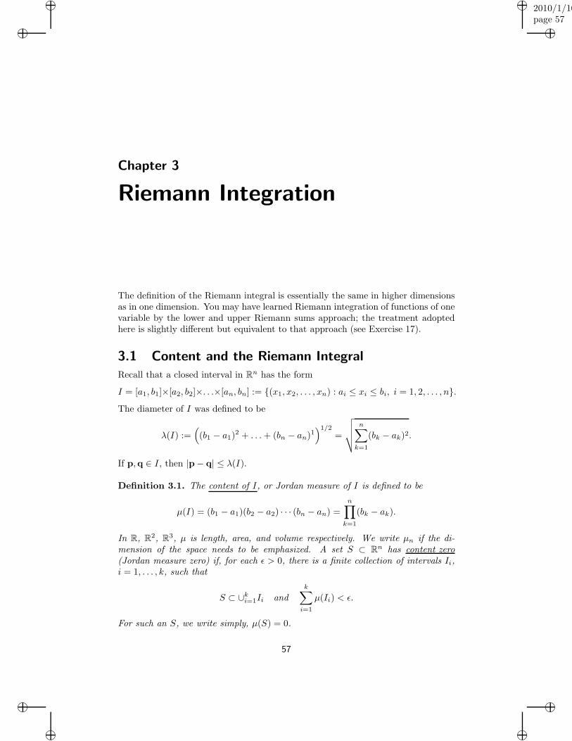
“muldowney”2010/1/10page 57
i
i
i
i
i
i
i
i
Chapter 3
Riemann Integration
The definition of the Riemann integral is essentially the same in higher dimensionsas in one dimension. You may have learned Riemann integration of functions of onevariable by the lower and upper Riemann sums approach; the treatment adoptedhere is slightly different but equivalent to that approach (see Exercise 17).
3.1 Content and the Riemann Integral
Recall that a closed interval in Rn has the form
I = [a1, b1]×[a2, b2]×. . .×[an, bn] := {(x1, x2, . . . , xn) : ai ≤ xi ≤ bi, i = 1, 2, . . . , n}.The diameter of I was defined to be
λ(I) :=((b1 − a1)
2 + . . .+ (bn − an)1)1/2
=
√√√√n∑
k=1
(bk − ak)2.
If p,q ∈ I, then |p− q| ≤ λ(I).
Definition 3.1. The content of I, or Jordan measure of I is defined to be
µ(I) = (b1 − a1)(b2 − a2) · · · (bn − an) =
n∏
k=1
(bk − ak).
In R, R2, R3, µ is length, area, and volume respectively. We write µn if the di-mension of the space needs to be emphasized. A set S ⊂ Rn has content zero(Jordan measure zero) if, for each ǫ > 0, there is a finite collection of intervals Ii,i = 1, . . . , k, such that
S ⊂ ∪ki=1Ii and
k∑
i=1
µ(Ii) < ǫ.
For such an S, we write simply, µ(S) = 0.
57
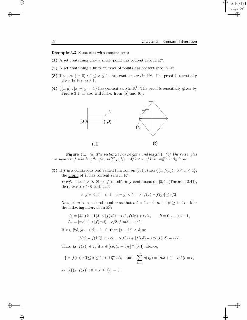
“muldowney”2010/1/10page 58
i
i
i
i
i
i
i
i
58 Chapter 3. Riemann Integration
Example 3.2 Some sets with content zero:
(1) A set containing only a single point has content zero in Rn.
(2) A set containing a finite number of points has content zero in Rn.
(3) The set {(x, 0) : 0 ≤ x ≤ 1} has content zero in R2. The proof is essentiallygiven in Figure 3.1.
(4) {(x, y) : |x|+ |y| = 1} has content zero in R2. The proof is essentially given byFigure 3.1. It also will follow from (5) and (6).
ε
(0,0) (1,0)1/k
(b) (α)
Figure 3.1. (a) The rectangle has height ǫ and length 1. (b) The rectanglesare squares of side length 1/k, so
∑µ(Ii) = 4/k < ǫ, if k is sufficiently large.
(5) If f is a continuous real valued function on [0, 1], then {(x, f(x)) : 0 ≤ x ≤ 1},the graph of f , has content zero in R2.
Proof. Let ǫ > 0. Since f is uniformly continuous on [0, 1] (Theorem 2.41),there exists δ > 0 such that
x, y ∈ [0, 1] and |x− y| < δ =⇒ |f(x)− f(y)| ≤ ǫ/2.
Now let m be a natural number so that mδ < 1 and (m+ 1)δ ≥ 1. Considerthe following intervals in R2:
Ik = [kδ, (k + 1)δ]× [f(kδ)− ǫ/2, f(kδ) + ǫ/2], k = 0, . . . ,m− 1,
Im = [mδ, 1]× [f(mδ)− ǫ/2, f(mδ) + ǫ/2].
If x ∈ [kδ, (k + 1)δ] ∩ [0, 1], then |x− kδ| < δ, so
|f(x)− f(kδ)| ≤ ǫ/2 =⇒ f(x) ∈ [f(kδ)− ǫ/2, f(kδ) + ǫ/2].
Thus, (x, f(x)) ∈ Ik if x ∈ [kδ, (k + 1)δ] ∩ [0, 1]. Hence,
{(x, f(x)) : 0 ≤ x ≤ 1} ⊂ ∪mk=1Ik andm∑
k=1
µ(Ik) = (mδ + 1−mδ)ǫ = ǫ,
so µ({(x, f(x)) : 0 ≤ x ≤ 1}
)= 0.
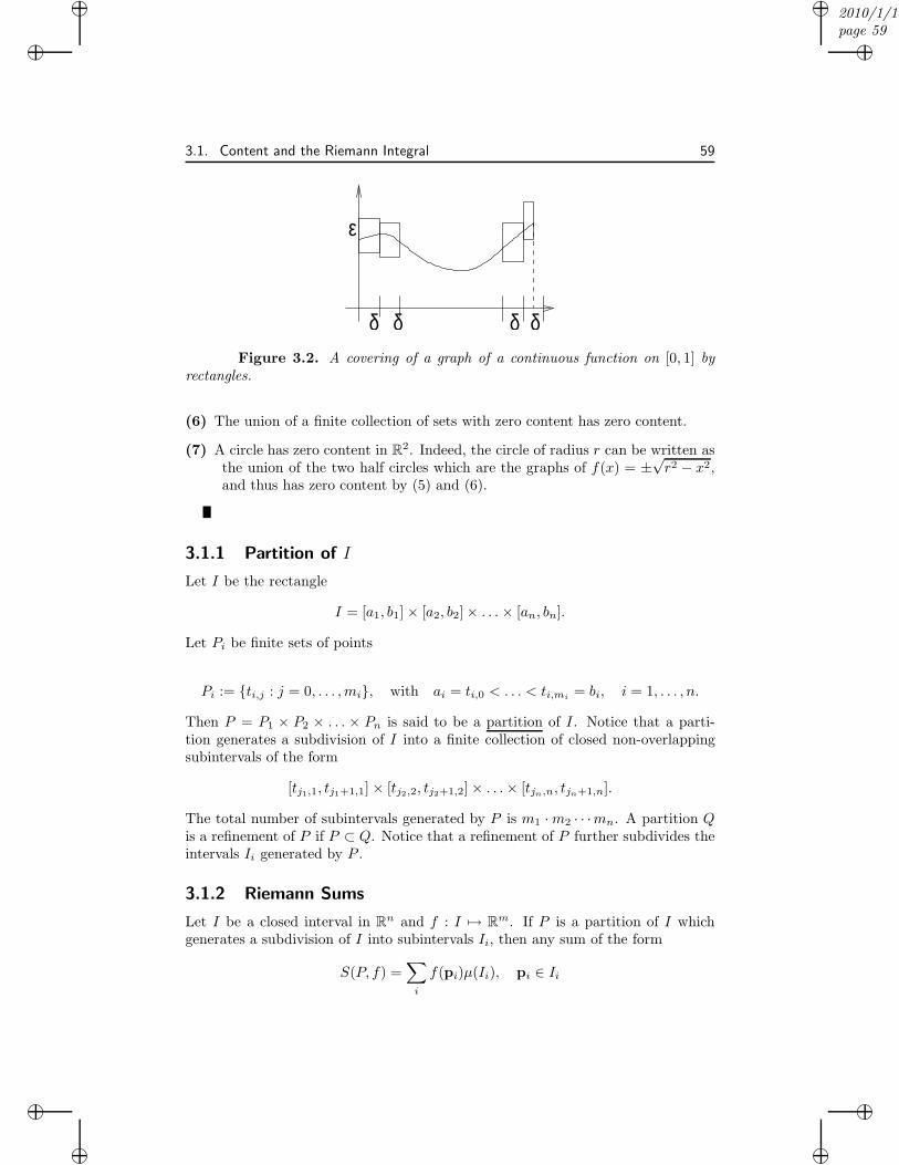
“muldowney”2010/1/10page 59
i
i
i
i
i
i
i
i
3.1. Content and the Riemann Integral 59
δ δ δ
ε
δFigure 3.2. A covering of a graph of a continuous function on [0, 1] by
rectangles.
(6) The union of a finite collection of sets with zero content has zero content.
(7) A circle has zero content in R2. Indeed, the circle of radius r can be written asthe union of the two half circles which are the graphs of f(x) = ±
√r2 − x2,
and thus has zero content by (5) and (6).
3.1.1 Partition of I
Let I be the rectangle
I = [a1, b1]× [a2, b2]× . . .× [an, bn].
Let Pi be finite sets of points
Pi := {ti,j : j = 0, . . . ,mi}, with ai = ti,0 < . . . < ti,mi= bi, i = 1, . . . , n.
Then P = P1 × P2 × . . . × Pn is said to be a partition of I. Notice that a parti-tion generates a subdivision of I into a finite collection of closed non-overlappingsubintervals of the form
[tj1,1, tj1+1,1]× [tj2,2, tj2+1,2]× . . .× [tjn,n, tjn+1,n].
The total number of subintervals generated by P is m1 ·m2 · · ·mn. A partition Qis a refinement of P if P ⊂ Q. Notice that a refinement of P further subdivides theintervals Ii generated by P .
3.1.2 Riemann Sums
Let I be a closed interval in Rn and f : I 7→ Rm. If P is a partition of I whichgenerates a subdivision of I into subintervals Ii, then any sum of the form
S(P, f) =∑
i
f(pi)µ(Ii), pi ∈ Ii
“muldowney”2010/1/10page 60
i
i
i
i
i
i
i
i
60 Chapter 3. Riemann Integration
II i
Figure 3.3. A covering of a graph of a continuous function on [0, 1] byrectangles.
is a Riemann sum of f corresponding to the partition P .
Definition 3.3 (Riemann Integral). Let f : I 7→ Rm where I is a closed intervalin Rn. Let α ∈ Rm. If, for each ǫ > 0, there is a partition Pǫ of I such that ifP ⊃ Pǫ and S(P, f) is any Riemann sum corresponding to P , then
|S(P, f)− α| < ǫ,
and the function f is said to be Riemann integrable on I and to have Riemannintegral α. We write
α =
∫
I
f or α =
∫
I
f dµ.
Proposition 3.4. If f is Riemann integrable on I, then the integral of f on I isunique.
Proof. Suppose α1 =∫If and α2 =
∫If . Let ǫ > 0 be given. Then there are
partitions P1,ǫ, P2,ǫ of I such that
P ⊃ Pi,ǫ =⇒ |S(P, f)− αi| < ǫ/2, i = 1, 2.
But the partition P1 ∪ P2 ⊃ P1 and P1 ∪ P2 ⊃ P2, so that
|α1 − α2| ≤ |S(P1 ∪ P2, f)− α1)|+ |S(P1 ∪ P2, f)− α2| ≤ ǫ/2 + ǫ/2 = ǫ.
We have thus shown |α1−α2| < ǫ for each ǫ > 0. Hence,|α1−α2| = 0, i.e. α1 = α2.
Exercises
3.1. If f is integrable on I, then f is bounded on I.
“muldowney”2010/1/10page 61
i
i
i
i
i
i
i
i
3.2. Cauchy Criteria and Properties of Integrals 61
3.2. f : I 7→ Rm is integrable on I if and only if each component function fi,i = 1, . . . ,m, of f is integrable on I. Moreover,
∫
I
f =
(∫
I
f1, . . . ,
∫
I
fm
).
It therefore suffices to consider only real-valued functions, just as in the caseof sequences.
3.2 Cauchy Criteria and Properties of Integrals
Theorem 3.5 (Cauchy Criterion). Let f : I 7→ Rm.∫I f exists if and only if
for each ǫ > 0 there exists a partition Pǫ of I such that if P,Q ⊃ Pǫ, then
|S(P, f)− S(Q, f)| < ǫ
for all Riemeann sums S(P, f), S(Q, f) corresponding to P ,Q.
Proof. “=⇒” If α =∫If exists, then for each ǫ > 0 there is a partition Pǫ of I
such that if P ⊃ Pǫ, then|S(P, f)− α| < ǫ/2. (3.1)
Let P,Q ⊃ Pǫ, then (3.1) implies
|S(P, f)− S(Q, f)| ≤ |S(P, f)− α|+ |α− S(Q, f)| < ǫ
2+ǫ
2= ǫ,
that is, the Cauchy Criterion is satisfied.“⇐=” Suppose the Cauchy Criterion is satisfied. There exist partitions Pk of
I such that P,Q ⊃ Pk implies
|S(P, f)− S(Q, f)| < 1
k, k = 1, 2, . . . . (3.2)
Let Qk = ∪kj=1Pj , for each k = 1, 2, . . ., and consider a fixed Riemann sumS0(Qk, f). If ℓ,m ≥ k, then Qm ⊃ Pk and Qℓ ⊃ Pk so, from (3.2),
|S0(Qℓ, f)− S0(Qm, f)| < 1
k, ∀ ℓ,m ≥ k.
Thus, {S0(Qk, f)} is a Cauchy sequence in Rm so
limk→∞
S0(Qk, f) = α exists. (3.3)
It remains to show that α =∫I f (Theorem 2.20). From (3.3) it follows that, if
ǫ > 0, there is a natural number N such that
1
N<ǫ
2and |S0(QN , f)− α| < ǫ
2. (3.4)
“muldowney”2010/1/10page 62
i
i
i
i
i
i
i
i
62 Chapter 3. Riemann Integration
If P is any refinement of QN , then both P and QN are refinements of PN (from thedefinition of QN ), so each Riemann sum S(P, f) satisfies
|S(P, f)− α| ≤ |S(P, f)− S0(QN , f)|+ |S0(QN , f)− α| < 1
N+ǫ
2<ǫ
2+ǫ
2.
by (3.2) and (3.4).
Lemma 3.6. Let I be an interval in Rn. If P is a partition of I into a finitecollection of non-overlapping subintervals {Ii}, then
µ(I) =∑
i
µ(Ii).
Proof. This can be proved by a straightforward induction on the number of subin-tervals into which I is partitioned. Do it.
The next corollary gives an equivalent but more readily applicable version ofthe Cauchy Criterion.
Corollary 3.7 (Cauchy Criterion).∫If exists if and only if for each ǫ > 0,
there exists a partition Pǫ such that if S1(Pǫ, f) and S2(Pǫ, f) are any two Riemannsums corresponding to Pǫ, then
|S1(Pǫ, f)− S2(Pǫ, f)| < ǫ.
Proof. It is evident from Theorem 3.5 that the condition is necessary. To see thatit is sufficient, let Pǫ satisfy the requirement of Corollary 3.7, and let P and Q berefinements of Pǫ, generating subintervals {Ak} and {Bj} respectively. Then
|S(P, f)− S(Q, f)| =∣∣∣∑k f(pk)µ(Ak)−
∑j f(qj)µ(Bj)
∣∣∣=
∣∣∣∑i
[∑Ak⊂Ii
f(pk)µ(Ak)−∑Bj⊂Ii
f(qj)µ(Bj)]∣∣∣(3.5)
where Ii are the subintervals generated by Pǫ. Now there exists points xi,x∗i in Ii
such that∣∣∣∣∣∣
∑
Ak⊂Ii
f(pk)µ(Ak)−∑
Bj⊂Ii
f(qj)µ(Bj)
∣∣∣∣∣∣≤(f(xi)− f(x∗
i ))µ(Ii). (3.6)
Indeed, to see that (3.6) is true, let
f(xi) = maxk,j{f(pk), f(qj)}, and f(x∗
i ) = mink,j{f(pk), f(qj)},
“muldowney”2010/1/10page 63
i
i
i
i
i
i
i
i
3.2. Cauchy Criteria and Properties of Integrals 63
where the max and min are taken over the k and j for which Ak ⊂ Ii and Bj ⊂ Ii,two finite sets. Then
f(x∗)∑
Ak⊂Ii
µ(Ai)− f(xi)∑
Bj⊂Ii
µ(Bj) ≤∑
Ak⊂Ii
f(pk)µ(Ak)−∑
Bj⊂Ii
f(qj)µ(Bj)
≤ f(xi)∑
Ak⊂Ii
µ(Ai)− f(x∗)∑
Bj⊂Ii
µ(Bj)
and (from the lemma)
∑
Ak⊂Ii
µ(Ai) =∑
Bj⊂Ii
µ(Bj) = µ(Ii)
so (3.6) follows.From (3.5) and (3.6), we find
|S(P, f)− S(Q, f)| ≤∑
i
[f(xi)− f(x∗i )]µ(Ii) = |S1(Pǫ, f)− S2(Pǫ, f)| < ǫ.
Thus, the Cauchy Criterion for integrability of f (as proved in Theorem 3.5) issatisfied, i.e.
∫If exists.
Theorem 3.8. If f is a continuous real-valued function on I, then∫If exists.
Proof. Since I is compact (why?), f is uniformly continuous on I (Theorem 2.41).If ǫ > 0 is given, there is a δ > 0 such that |p−q| < δ implies |f(p)−f(q)| < ǫ/µ(I).We may choose a partition Pǫ sufficiently fine to ensure that the subintervals Iiwhich it generates have diameter
λ(Ii) < δ.
Hence, if p,q ∈ Ii, then
|p− q| ≤ λ(Ii) < δ =⇒ |f(p)− f(q)| < ǫ/µ(I),
and consequently, when S1(Pǫ, f) and S2(Pǫ, f) are any two Riemann sums corre-sponding to Pǫ, we have
|S1(Pǫ, f)− S2(Pǫ, f)| =∣∣∣∣∣∑
i
(f(pi)− f(qi)
)µ(Ii)
∣∣∣∣∣
≤∑
i
|f(pi)− f(qi)|)µ(Ii) <ǫ
µ(I)
∑
i
µ(Ii) =ǫ
µ(I)µ(I) = ǫ.
Thus,∫I f exists by the Cauchy Criterion (Corollary 3.7).
Theorem 3.9. Suppose that
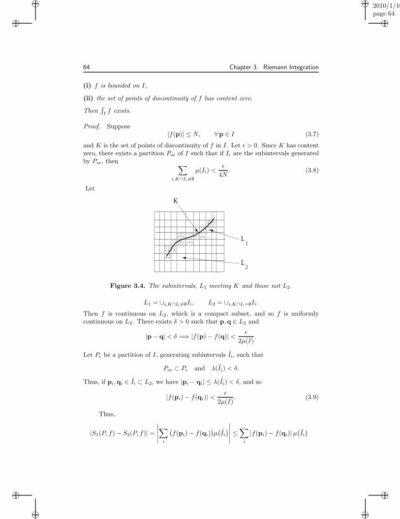
“muldowney”2010/1/10page 64
i
i
i
i
i
i
i
i
64 Chapter 3. Riemann Integration
(i) f is bounded on I,
(ii) the set of points of discontinuity of f has content zero.
Then∫I f exists.
Proof. Suppose|f(p)| ≤ N, ∀p ∈ I (3.7)
and K is the set of points of discontinuity of f in I. Let ǫ > 0. Since K has contentzero, there exists a partition Poǫ of I such that if Ii are the subintervals generatedby Poǫ, then ∑
i,K∩Ii 6=∅µ(Ii) <
ǫ
4N. (3.8)
Let
L
L
K
2
1
Figure 3.4. The subintervals, L1 meeting K and those not L2.
L1 = ∪i,K∩Ii 6=∅Ii, L2 = ∪i,K∩Ii=∅Ii.
Then f is continuous on L2, which is a compact subset, and so f is uniformlycontinuous on L2. There exists δ > 0 such that p,q ∈ L2 and
|p− q| < δ =⇒ |f(p)− f(q)| < ǫ
2µ(I).
Let Pǫ be a partition of I, generating subintervals Ii, such that
Poǫ ⊂ Pǫ and λ(Ii) < δ.
Thus, if pi,qi ∈ Ii ⊂ L2, we have |pi − qi| ≤ λ(Ii) < δ, and so
|f(pi)− f(qi)| <ǫ
2µ(I). (3.9)
Thus,
|S1(P, f)− S2(P, f)| =∣∣∣∣∣∑
i
(f(pi)− f(qi)
)µ(Ii)∣∣∣∣∣ ≤
∑
i
|f(pi)− f(qi)|µ(Ii)
“muldowney”2010/1/10page 65
i
i
i
i
i
i
i
i
3.2. Cauchy Criteria and Properties of Integrals 65
≤∑
Ii⊂L1
|f(pi)− f(qi)|µ(Ii)
+∑
Ii⊂L2
|f(pi)− f(qi)|µ(Ii)
< 2N∑
Ii⊂L1
µ(Ii) +
ǫ
2µ(I)
∑
Ii⊂L2
µ(Ii)
≤ 2Nǫ
4N+
ǫ
2µ(I)µ(I) = ǫ
by (3.7), (3.8), and (3.9). Thus, f satisfies the Cauchy Criterion (Corollary 3.7)and
∫If exists.
Example 3.10 Let f(x, y) = xy2, 0 ≤ x ≤ 1, 0 ≤ y ≤ 1 and I = [0, 1] × [0, 1].Then f is continuous on I so
∫I f exists. Partition I into k2 intervals of side length
1k :
Pk :=
{Ii,j =
[i− 1
k,i
k
]×[j − 1
k,j
k
], i = 1, . . . , k, j = 1, . . . , k
}.
If pi,j ∈ Ii,j , then i−1k
(j−1k
)2 ≤ f(pi,j) ≤ ik
(jk
)2, so that
k∑
i,j=1
i− 1
k
(j − 1
k
)21
k2≤ S(Pk, f) ≤
k∑
i,j=1
i
k
(j
k
)21
k2
and the same estimate holds for any S(P, f) if P ⊃ Pk. Now
1
k2
k∑
i,j=1
i− 1
k
(j − 1
k
)2
=1
k5
k−1∑
i=1
i
k−1∑
j=1
j2
=1
k5
k(k − 1)
2
(k − 1)k(2k − 1)
6→ 1
6
1
k2
k∑
i,j=1
i
k
(j
k
)2
=1
k5
k∑
i=1
ik∑
j=1
j2
=1
k5
k(k + 1)
2
k(k + 1)(2k + 1)
6→ 1
6.
Thus,∫If = 1
6 .
Definition 3.11. Suppose that
(i) D is a bounded subset of Rn (so D ⊂ I for some closed interval I in Rn)
(ii) f : D 7→ R.
Extend the domain of f by defining f(p) = 0 if p 6∈ D. Then we say that∫D f
exists if and only if∫If exists and define
∫
D
f =
∫
I
f.
“muldowney”2010/1/10page 66
i
i
i
i
i
i
i
i
66 Chapter 3. Riemann Integration
Theorem 3.12. Suppose
(i) D is bounded and the boundary of D, ∂D, has content zero,
(ii) f is continuous and bounded on D.
Then∫D
exists.
Proof. The function f with its domain extended to the interval I ⊃ D as in theprevious definition, is continuous at each point of I except possibly at points in∂D. But µ(∂D) = 0, so by Theorem 3.9,
∫I f exists. Therefore,
∫D f exists and, by
definition, is equal to∫If .
Definition 3.13. A bounded set D ⊂ Rn has content if∫D 1 exists and
µ(D) :=
∫
D
1.
Equivalently, we define the characteristic function χD of D by
χD(p) =
{1, if p ∈ D;0, if p 6∈ D,
and let I be any closed interval containing D as a subset. Then D has content if∫IχD exists and then
µ(D) :=
∫
I
χD.
Theorem 3.14. A bounded subset D ⊂ Rn has content if and only if µ(∂D) = 0.
Proof. Exercise 4.
Theorem 3.15 (Properties of the Integral).
(a) If∫Df and
∫Dg exist and α, β ∈ R, then
∫D
(αf + βg) exists.
(b) If f(p) ≥ 0 for all p ∈ D and∫D f exists, then
∫
D
f ≥ 0.
(c) If∫D f exists, then
∫D |f | exists, and
∣∣∣∣∫
D
f
∣∣∣∣ ≤∫
D
|f |.
“muldowney”2010/1/10page 67
i
i
i
i
i
i
i
i
3.2. Cauchy Criteria and Properties of Integrals 67
(d) If∫D1f and
∫D2f exist, and µ(D1 ∩D2) = 0, then
∫
D1∪D2
f =
∫
D1
f +
∫
D2
f.
(e) If (i) D has content, (ii)∫Df exists, and (iii) m ≤ f(p) ≤ M for all p ∈ D,
then
mµ(D) ≤∫
D
f ≤Mµ(D).
(f) (Mean Value theorem for Integrals). If D is a compact connected set withcontent (i.e.µ(∂D) = 0), and f is continuous on D, then there exists p0 ∈ Dsuch that ∫
D
f = f(p0)µ(D).
Proof. (a) There is no loss of generality by assuming D is an interval in this case.Let ǫ > 0 be given. Then
1.∫Df exists implies there exists a partition P1,ǫ of D such that for P ⊃ P1,ǫ,
|S(P, f)−∫D f | < ǫ.
2.∫D g exists implies there exists a partition P2,ǫ of D such that for P ⊃ P2,ǫ,|S(P, f)−
∫Dg| < ǫ.
Let Pǫ = P1,ǫ ∪ P2,ǫ. Then if P ⊃ Pǫ, we have∣∣∣∣S(P, αf + βg)− α
∫
D
f − β∫
D
g
∣∣∣∣ =∣∣∣∣αS(P, f) + βS(P, g)− α
∫
D
f − β∫
D
g
∣∣∣∣
≤ |α|∣∣∣∣S(P, f)−
∫
D
f
∣∣∣∣+ |β|∣∣∣∣S(P, g)−
∫
D
g
∣∣∣∣≤ (|α|+ |β|)ǫ.
Thus,∫D(αf + βg) exists and equals α
∫D f + β
∫D g.
Proof of (b). Exercise 6Proof of (c). Exercise 7Proof of (d): Let χDi
be the characteristic functions of Di, i = 1, 2, and let Ibe a closed interval containing D1 ∪D2. By definition
∫
D1
f =
∫
I
fχD1=
∫
D1∪D2
fχD1
∫
D2
f =
∫
I
fχD2=
∫
D1∪D2
fχD2
By part (a) of the present Theorem,∫D1∪D2
f(χD1+ χD2
) exists and
∫
D1∪D2
f(χD1+ χD2
) =
∫
D1∪D2
fχD1+
∫
D1∪D2
fχD2=
∫
D1
f +
∫
D2
f.
“muldowney”2010/1/10page 68
i
i
i
i
i
i
i
i
68 Chapter 3. Riemann Integration
From Exercise 3 and the fact that
f(p)(χD1(p) + χD2
(p))χD1∪D2(p) = f(p)χD1∪D2
(p),
{p 6∈ D1 ∩D2, withµ(D1 ∩D2) = 0,
then also by definition we have
∫
D1∪D2
f(χD1+ χD2
) =
∫
I
f(χD1+ χD2
)χD1∪D2
=
∫
I
fχD1∪D2=
∫
D1∪D2
f.
Thus,∫D1∪D2
f exists and equals∫D1f +
∫D2f .
Proof of (e): Exercise 8.Proof of (f): There will be two cases.Case (i): If µ(D) = 0, then since mµ(D) = M µ(D) = 0, by part (e) we have
∫
D
f = 0 =⇒∫
D
f = f(p0)µ(D), ∀p0 ∈ D.
Case (ii): If µ(D) 6= 0, then by (e)
{m := inf{f(p) : p ∈ D}M := sup{f(p) : p ∈ D} =⇒ m ≤
∫Df
µ(D)≤M.
By Corollary 2.38, D compact and f continuous on D implies that there exist pointsp1,p2 ∈ D with f(p1) = m and f(p2) = M . Therefore, by Corollary 2.34 (theIntermediate Value Theorem), there exists p0 ∈ D such that
f(p0) =
∫Df
µ(D)=⇒ f(p0)µ(D) =
∫
D
f.
Discussion: A subset of Rn has Jordan measure zero if, for each ǫ > 0, there is afinite collection of intervals {Ik} such that
K ⊂ ∪kIk and∑
k
µ(Ik) ≤ ǫ.
K has Lebesgue measure zero if, for each ǫ > 0, there is a countable collectionof intervals {Ik} satisfying the displayed relation. This simple extension of theconcept of measure zero has profound consequences. We know that the set ofrationals in [0, 1] does not have Jordan content. However, if this set is enumeratedas {rk : k = 1, 2, 3, . . .}, then rk ∈ Ik with µ(Ik) = ǫ
2k yields
{rk : k = 1, 2, 3, . . .} ⊂ ∪kIk and∑
k
µ(Ik) = ǫ
∞∑
k=1
1
2k= ǫ.
“muldowney”2010/1/10page 69
i
i
i
i
i
i
i
i
3.2. Cauchy Criteria and Properties of Integrals 69
Thus the set of rationals in [0, 1] has Lebesgue measure zero. In fact, the sameargument shows that Q, or any countable set of real numbers has Lebesgue measurezero. Countable sets are not the only sets of Lebesgue measure zero however; infact, they can be quite complicated. The remarkable Cantor set which you willstudy in Real Analysis has Lebesgue measure zero but nonetheless has the samecardinality as [0, 1], i.e. it has zero “length” but has the same “number” of pointsas [0, 1]. A simple discussion of the Cantor set can be found in Bartle’s book.
An interesting theorem of Lebesgue states that, for a bounded real-valuedfunction f , the Riemann integral
∫If exists if and only if the set of points in I at
which f is discontinuous has Lebesgue measure zero. For example, for the functionsin Exercises 15 and 16, the one in the first exercise is discontinuous at each point in[0, 1], while the function in the second exercise is only discontinuous at the rationalpoints in [0, 1]
Exercises
3.3. Suppose f and g are bounded on I and f(p) = g(p) for all p ∈ I\K, whereK has content zero. Prove that
∫
I
f exists =⇒∫
I
g exists and equals
∫
I
f.
3.4. Prove Theorem 3.14.
3.5. Give an example of a countable set which has content and one which doesnot have content (contented and discontented sets??). Is there a countableset with positive content?
3.6. Prove Theorem 3.15 (b).
3.7. Prove Theorem 3.15 (c).
3.8. Prove Theorem 3.15 (e). Hint: Use parts (a) and (b).
3.9. Prove that {( 1m ,
1k ) : m, k = 1, 2, . . .} has content zero in R2.
3.10. Prove that the set of points in [0, 1]× [0, 1] with rational coordinates does nothave content in R2.
3.11. Let D be a subset of Rn which has content zero and f be any boundedfunction on D. Prove that
∫D f exists and equals zero.
3.12. Let D be any bounded subset of Rn and f(p) = 0 for all p ∈ D. Prove that∫D f exists and equals 0. Note that D does not necessarily have content.
3.13. Show that∫ 1
0 sin( 1x ) dx exists and is independent of the value assigned to the
integrand at x = 0.
3.14. If∫D f exists and D1 is any subset of D with content, then
∫D1f exists
(D itself does not necessarily have content). Note that this exercise proves
in particular that the existence∫ ba f implies the existence of
∫ ca f for any
c ∈ (a, b).

“muldowney”2010/1/10page 70
i
i
i
i
i
i
i
i
70 Chapter 3. Riemann Integration
3.15. If f(x) = 0, x 6∈ Q and f(x) = 1 for x ∈ Q, then f is not Riemann integrableon [0, 1].
3.16. If
f(x) =
{0, if x 6∈ Q1q , if x = p
q and gcd(p, q) = 1,
then∫ 1
0f = 0.
3.17. If P is a partition of the interval I and f : I 7→ R, f bounded, defineS(P, f) and S(P, f), the lower and upper Riemann sums corresponding tothe partition P to be inf{S(P, f)} and sup{S(P, f)} repectively, the inf andsup being taken over all Riemann sums corresponding to the partition P andthe function f . Let
∫
I
f = supP{S(P, f)} and
∫
I
f = inf P{S(P, f)},
the sup and inf here being taken over all partitions P of I.
(i) Show that Q ⊃ P implies
S(P, f) ≤ S(Q, f) ≤ S(Q, f) ≤ S(P, f).
(ii) Show that∫If ≤
∫If .
(iii) (Definition). f is integrable on I if∫If =
∫If , and then we define
∫
I
f =
∫
I
f =
∫
I
f.
(iv) Show that f is integrable in this sense if and only if there is exactly onenumber α such that
S(P, f) ≤ α ≤ S(P, f)
for every partition P of I, in which case∫If = α.
(v) (Cauchy Criterion). Show that∫If exists in this sense if and only if, for
each ǫ > 0, there exists a partition Pǫ of I such that
|S(Pǫ, f)− S(Pǫ, f)| < ǫ.
(vi) Show that for a bounded f , f is integrable on I in the sense of (iii) ifand only if f is integrable in the sense adopted in these notes and thatboth definitions give the same value for
∫I f .
“muldowney”2010/1/10page 71
i
i
i
i
i
i
i
i
3.3. Evaluation of Integrals 71
3.3 Evaluation of Integrals
3.3.1 Real valued functions of a real variable
Theorem 3.16 (Fundamental Theorem of Calculus). If f is continuous on[a, b], then there is a function F on [a, b] such that
F ′(x) = f(x), a ≤ x ≤ b.
Proof. Consider the function F (x) =∫ xa f , a ≤ x ≤ b which exists by Exercise 14,
we have from Theorem 3.15 (d) and (f) that
F (x+ h)− F (x) =
∫ x+h
x
f = f(ch)h,
where ch is in the interval between x and x+ h. Since f is continuous on [a, b],
limh→0
F (x+ h)− F (x)
h= lim
h→0f(ch) = f(x).
Any function F with the property that F ′(x) = f(x), a ≤ x ≤ b, is called anantiderivative of f on [a, b].
Proposition 3.17. If F1 and F2 are antiderivatives of f , then F1−F2 is a constantfunction.
Proof. F ′1(x)− F ′
2(x) = f(x)− f(x) = 0, for all x. Therefore, F1 −F2 is constant.
Theorem 3.18. If f is continuous on [a, b] and F is any antiderivative of f on[a, b], then ∫ b
a
f = F (b)− F (a).
Proof. By the proceding Proposition, there is a constant C so that∫ xaf = F (x)−
C. When x = a, this yields∫ aaf = 0 = F (a) − C, while using this when x = b we
find∫ ba f = F (b)− C = F (b)− F (a).
Corollary 3.19 (Change of Variable Formula). Suppose that
(i) φ′ exists and is continuous on [a, b].
(ii) f is continuous on φ([a, b]).
“muldowney”2010/1/10page 72
i
i
i
i
i
i
i
i
72 Chapter 3. Riemann Integration
Then
∫ φ(b)
φ(a)
f =
∫ b
a
(f ◦ φ)φ′, or
∫ φ(b)
φ(a)
f(x) dx =
∫ b
a
f(φ(u))φ′(u) du.
Proof. If F is an antiderivative of f , then
d
duF (φ(u)) = f(φ(u))φ′(u),
so that F ◦ φ is an antiderivative of (f ◦ φ)φ′. Therefore,
∫ φ(b)
φ(a)
f = F (φ(b))− F (φ(a)) =
∫ b
a
(f ◦ φ)φ′.
You will have noticed that we used the Chain Rule here even though it wasnot yet proven in these Notes. A proof will be given in the next chapter in a moregeneral context.
Example 3.20 To evaluate∫ π/20
sin2(u) cos(u) du, we take f(x) = x2, φ(u) =sin(u), and φ′(u) = cos(u). Then
∫ π/2
0
sin2(u) cos(u) du =
∫ φ(π/2)
φ(0)
x2 dx =
∫ 1
0
x2 dx =1
3.
Corollary 3.21 (Integration by Parts Formula). If f ′ and g′ are continuouson [a, b]. then
∫ b
a
fg′ +
∫ b
a
f ′g = f(b)g(b)− f(a)g(a).
Proof. An antiderivative of fg′ + f ′g is fg. Therefore, the formula follows imme-diately.
Example 3.22
∫ 1
0
xex dx = xex∣∣∣1
0−∫ 1
0
ex dx = e− (ex∣∣∣1
0) = e− (e− 1) = 1.
“muldowney”2010/1/10page 73
i
i
i
i
i
i
i
i
3.3. Evaluation of Integrals 73
3.3.2 Real valued functions on R2
The important theorem of Fubini allows us to extend the use of the FundamentalTheorem of Calculus to functions of more than one variable.
Theorem 3.23 (Fubini’s Theorem). Let f : I = [a, b]× [c, d] 7→ R. Suppose that
(ii)∫If exists
(ii)∫ dcf(x, y) dy = F (x) exists for each x ∈ [a, b].
Then∫ baF (x) dx exists and
∫ b
a
F (x) dx =
∫ b
a
[∫ d
c
f(x, y) dy
]dx =
∫
I
f.
Proof. The definition of∫If states that if ǫ > 0 is given, there is a partition Pǫ of
I such that
P ⊃ Pǫ =⇒∣∣∣∣S(P, f)−
∫
I
f
∣∣∣∣ < ǫ,
for any Riemann sum S(P, f). Writing this in detail,
P = {x0, x1, . . . , xm} × {y0, y1, . . . , yk} ⊃ Pǫ
=⇒
∣∣∣∣∣∣
m∑
i=1
k∑
j=1
f(x∗i , y∗j )(xi − xi−1)(yj − yj−1)−
∫
I
f
∣∣∣∣∣∣< ǫ,
where xi−1 ≤ x∗i ≤ xi and yj−1 ≤ y∗j ≤ yj . This may be written as
∣∣∣∣∣∣
m∑
i=1
(xi − xi−1)
k∑
j=1
f(x∗i , y∗j )(yj − yj−1)−
∫
I
f
∣∣∣∣∣∣< ǫ. (3.10)
Condition (ii) implies that for any fixed set of numbers x∗i , i = 1, . . . ,m, the parti-tion {yj} of [c, d] may be chosen to be so fine that
∣∣∣∣∣∣
k∑
j=1
f(x∗i , y∗j )(yj − yj−1)−
∫ d
c
f(x∗i , y) dy
∣∣∣∣∣∣<
ǫ
b− a , i = 1, . . . ,m,
since each of the integrals∫ dc f(x∗i , y) dy exists. Therefore, for the x∗i we have
∣∣∣∣∣∣
k∑
j=1
f(x∗i , y∗j )(yj − yj−1)− F (x∗i )
∣∣∣∣∣∣<
ǫ
b− a , i = 1, . . . ,m. (3.11)
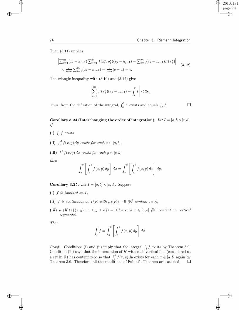
“muldowney”2010/1/10page 74
i
i
i
i
i
i
i
i
74 Chapter 3. Riemann Integration
Then (3.11) implies
∣∣∣∑mi=1(xi − xi−1)
∑kj=1 f(x∗i , y
∗j )(yj − yj−1)−
∑mi=1(xi − xi−1)F (x∗i )
∣∣∣
< ǫb−a
∑mi=1(xi − xi−1) = ǫ
b−a (b− a) = ǫ.(3.12)
The triangle inequality with (3.10) and (3.12) gives
∣∣∣∣∣
m∑
i=1
F (x∗i )(xi − xi−1)−∫
I
f
∣∣∣∣∣ < 2ǫ.
Thus, from the definition of the integral,∫ ba F exists and equals
∫I f .
Corollary 3.24 (Interchanging the order of integration). Let I = [a, b]×[c, d].If
(i)∫If exists
(ii)∫ dcf(x, y) dy exists for each x ∈ [a, b],
(iii)∫ ba f(x, y) dx exists for each y ∈ [c, d],
then ∫ b
a
[∫ d
c
f(x, y) dy
]dx =
∫ d
c
[∫ b
a
f(x, y) dx
]dy.
Corollary 3.25. Let I = [a, b]× [c, d]. Suppose
(i) f is bounded on I,
(ii) f is continuous on I\K with µ2(K) = 0 (R2 content zero),
(iii) µ1(K ∩ {(x, y) : c ≤ y ≤ d}) = 0 for each x ∈ [a, b] (R1 content on verticalsegments).
Then ∫
I
f =
∫ b
a
[∫ d
c
f(x, y) dy
]dx.
Proof. Conditions (i) and (ii) imply that the integral∫If exists by Theorem 3.9.
Condition (iii) says that the intersection of K with each vertical line (considered as
a set in R) has content zero so that∫ dc f(x, y) dy exists for each x ∈ [a, b] again by
Theorem 3.9. Therefore, all the conditions of Fubini’s Theorem are satisfied.
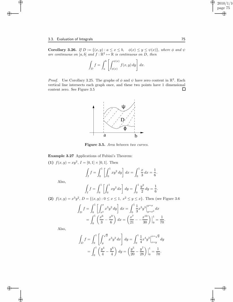
“muldowney”2010/1/10page 75
i
i
i
i
i
i
i
i
3.3. Evaluation of Integrals 75
Corollary 3.26. If D := {(x, y) : a ≤ x ≤ b, φ(x) ≤ y ≤ ψ(x)}, where φ and ψare continuous on [a, b] and f : R2 7→ R is continuous on D, then
∫
D
f =
∫ b
a
[∫ ψ(x)
φ(x)
f(x, y) dy
]dx.
Proof. Use Corollary 3.25. The graphs of φ and ψ have zero content in R2. Eachvertical line intersects each graph once, and these two points have 1 dimensionalcontent zero. See Figure 3.5
D
a b
ϕ
ψ
Figure 3.5. Area between two curves.
Example 3.27 Applications of Fubini’s Theorem:
(1) f(x, y) = xy2, I = [0, 1]× [0, 1]. Then∫
I
f =
∫ 1
0
[∫ 1
0
xy2 dy
]dx =
∫ 1
0
x
3dx =
1
6.
Also, ∫
I
f =
∫ 1
0
[∫ 1
0
xy2 dx
]dy =
∫ 1
0
y2
2dy =
1
6.
(2) f(x, y) = x3y2, D = {(x, y) : 0 ≤ x ≤ 1, x2 ≤ y ≤ x}. Then (see Figure 3.6∫
D
f =
∫ 1
0
[∫ x
x2
x3y2 dy
]dx =
∫ 1
0
1
3x3y3
∣∣∣y=x
y=x2dx
=
∫ 1
0
(x6
3− x9
6
)dx =
(x7
21−−x
10
30
)∣∣∣1
0=
1
70.
Also,
∫
D
f =
∫ 1
0
[∫ √y
y
x3y2 dx
]dy =
∫ 1
0
1
4x4y2
∣∣∣x=
√y
x=ydy
=
∫ 1
0
(y4
4− y6
4
)dy =
(y5
20− y7
28
) ∣∣∣1
0=
1
70.
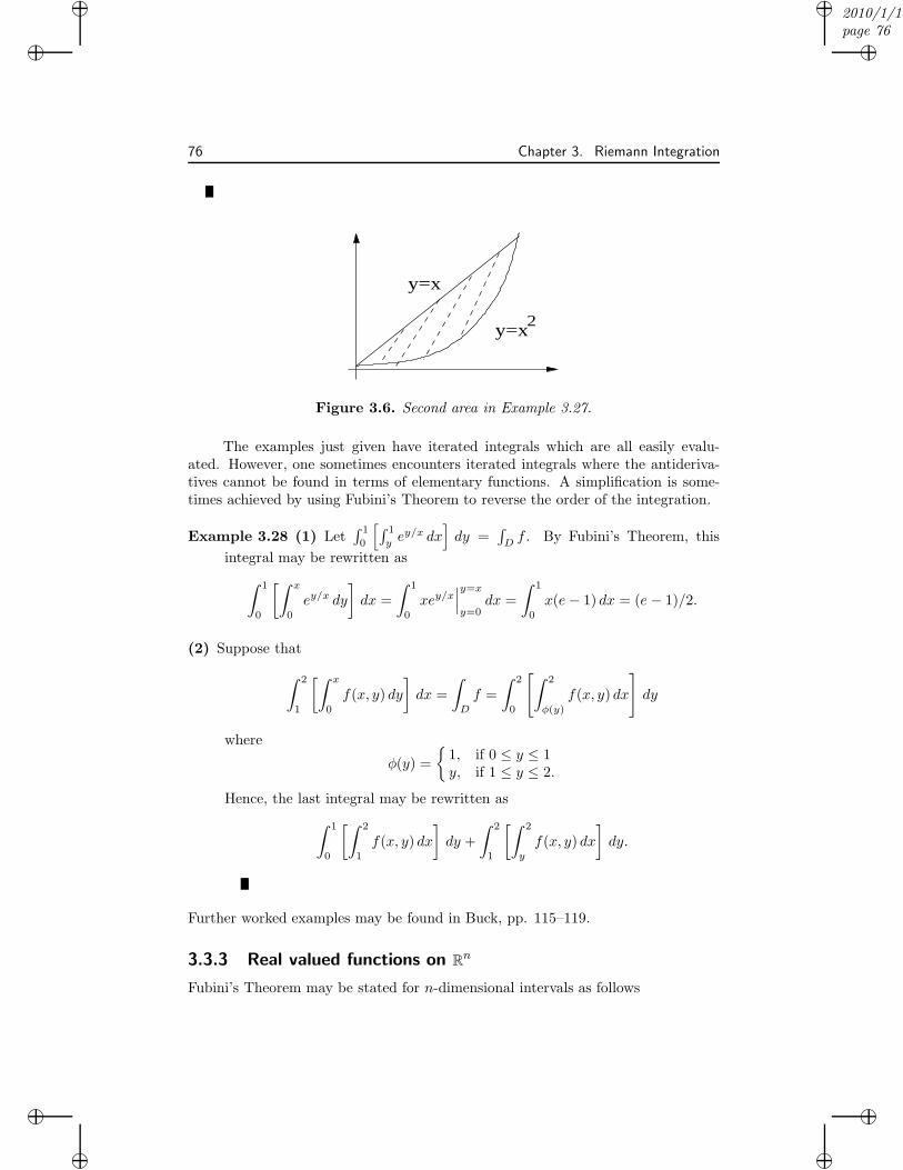
“muldowney”2010/1/10page 76
i
i
i
i
i
i
i
i
76 Chapter 3. Riemann Integration
y=x
y=x2
Figure 3.6. Second area in Example 3.27.
The examples just given have iterated integrals which are all easily evalu-ated. However, one sometimes encounters iterated integrals where the antideriva-tives cannot be found in terms of elementary functions. A simplification is some-times achieved by using Fubini’s Theorem to reverse the order of the integration.
Example 3.28 (1) Let∫ 1
0
[∫ 1
yey/x dx
]dy =
∫Df . By Fubini’s Theorem, this
integral may be rewritten as
∫ 1
0
[∫ x
0
ey/x dy
]dx =
∫ 1
0
xey/x∣∣∣y=x
y=0dx =
∫ 1
0
x(e− 1) dx = (e− 1)/2.
(2) Suppose that
∫ 2
1
[∫ x
0
f(x, y) dy
]dx =
∫
D
f =
∫ 2
0
[∫ 2
φ(y)
f(x, y) dx
]dy
where
φ(y) =
{1, if 0 ≤ y ≤ 1y, if 1 ≤ y ≤ 2.
Hence, the last integral may be rewritten as
∫ 1
0
[∫ 2
1
f(x, y) dx
]dy +
∫ 2
1
[∫ 2
y
f(x, y) dx
]dy.
Further worked examples may be found in Buck, pp. 115–119.
3.3.3 Real valued functions on Rn
Fubini’s Theorem may be stated for n-dimensional intervals as follows
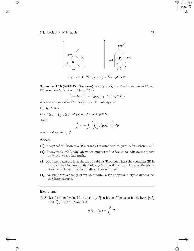
“muldowney”2010/1/10page 77
i
i
i
i
i
i
i
i
3.3. Evaluation of Integrals 77
y=0
x=1x=2
y=x
y=0
x=1
DD
y=x
Figure 3.7. The figures for Example 3.28.
Theorem 3.29 (Fubini’s Theorem). Let Iℓ and Im be closed intervals in Rℓ andRm respectively, with n = ℓ+m. Thus,
In = Iℓ × Im = {(p,q) : p ∈ Iℓ, q ∈ Im}is a closed interval in Rn. Let f : In 7→ R and suppose
(i)∫Inf exits
(ii) F (p) =∫Imf(p,q) dq exists for each p ∈ Iℓ.
Then ∫
Iℓ
F =
∫
Iℓ
[∫
Im
f(p,q) dq
]dp
exists and equals∫Inf .
Notes:
(1) The proof of Theorem 3.29 is exactly the same as that given before when n = 2.
(2) The symbols “dp”, “dq” above are simply used as devices to indicate the spaceson which we are integrating.
(3) For a more general formulation of Fubini’s Theorem where the condition (ii) isdropped see Calculus on Manifolds by M. Spivak (p. 58). However, the abovestatement of the theorem is sufficient for our needs.
(4) We will prove a change of variables formula for integrals in higher dimensionsin a later chapter.
Exercises
3.18. Let f be a real-valued function on [a, b] such that f ′(x) exists for each x ∈ [a, b]
and∫ baf ′ exists. Prove that
f(b)− f(a) =
∫ b
a
f ′.
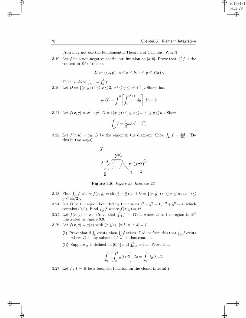
“muldowney”2010/1/10page 78
i
i
i
i
i
i
i
i
78 Chapter 3. Riemann Integration
(You may not use the Fundamental Theorem of Calculus. Why?)
3.19. Let f be a non-negative continuous function on [a, b]. Prove that∫ ba f is the
content in R2 of the set
D := {(x, y) : a ≤ x ≤ b, 0 ≤ y ≤ f(x)}.
That is, show∫D 1 =
∫ ba f .
3.20. Let D := {(x, y) : 1 ≤ x ≤ 3, x2 ≤ y ≤ x2 + 1}. Show that
µ(D) =
∫ 3
1
[∫ x2+1
x2
dy
]dx = 2.
3.21. Let f(x, y) = x2 + y2, D = {(x, y) : 0 ≤ x ≤ a, 0 ≤ y ≤ b}. Show
∫
D
f =1
3ab(a2 + b2).
3.22. Let f(x, y) = xy, D be the region in the diagram. Show∫D f = 131
120 . (Dothis in two ways).
0 4
y=(x−3)2
y=1
x
y
y=x
Figure 3.8. Figure for Exercise 22.
3.23. Find∫Df where f(x, y) = sin(xa + y
b ) and D = {(x, y) : 0 ≤ x ≤ πa/2, 0 ≤y ≤ πb/2}.
3.24. Let D be the region bounded by the curves x2 − y2 = 1, x2 + y2 = 4, whichcontains (0, 0). Find
∫Df where f(x, y) = x2.
3.25. Let f(x, y) = x. Prove that∫D f = 77/4, where D is the region in R2
illustrated in Figure 3.9.
3.26. Let f(x, y) = g(x) with (x, y) ∈ [a, b]× [c, d] = I.
(i) Prove that if∫ ba
exists, then∫If exists. Deduce from this that
∫Df exists
where D is any subset of I which has content.
(ii) Suppose g is defined on [0, 1] and∫ 1
0 g exists. Prove that
∫ 1
0
[∫ 1
x
g(t) dt
]dx =
∫ 1
0
tg(t) dt.
3.27. Let f : I 7→ R be a bounded function on the closed interval I.
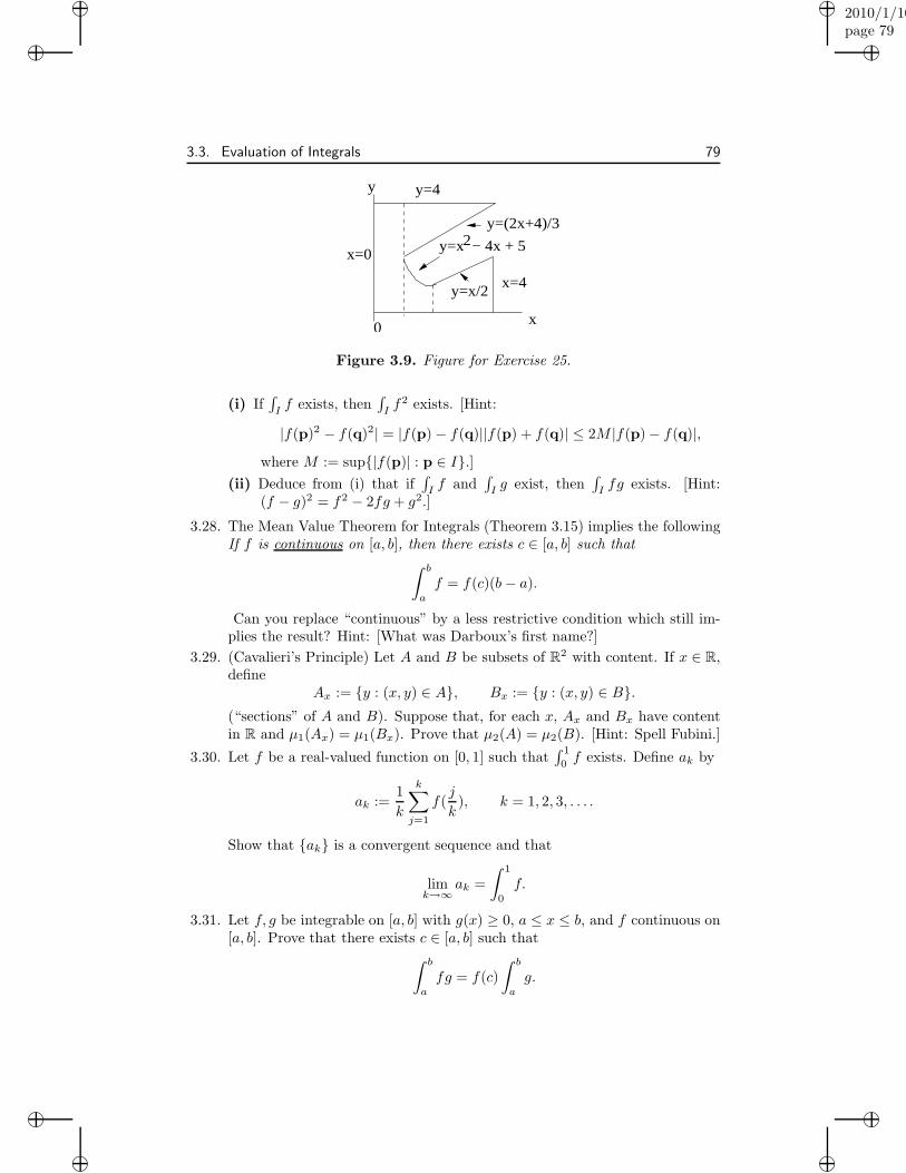
“muldowney”2010/1/10page 79
i
i
i
i
i
i
i
i
3.3. Evaluation of Integrals 79
������������
��
�������� x=4
y=4
y=(2x+4)/3
x
y
0
x=0
y=x/2
y=x − 4x + 52
Figure 3.9. Figure for Exercise 25.
(i) If∫If exists, then
∫If2 exists. [Hint:
|f(p)2 − f(q)2| = |f(p)− f(q)||f(p) + f(q)| ≤ 2M |f(p)− f(q)|,where M := sup{|f(p)| : p ∈ I}.]
(ii) Deduce from (i) that if∫I f and
∫I g exist, then
∫I fg exists. [Hint:
(f − g)2 = f2 − 2fg + g2.]
3.28. The Mean Value Theorem for Integrals (Theorem 3.15) implies the followingIf f is continuous on [a, b], then there exists c ∈ [a, b] such that
∫ b
a
f = f(c)(b − a).
Can you replace “continuous” by a less restrictive condition which still im-plies the result? Hint: [What was Darboux’s first name?]
3.29. (Cavalieri’s Principle) Let A and B be subsets of R2 with content. If x ∈ R,define
Ax := {y : (x, y) ∈ A}, Bx := {y : (x, y) ∈ B}.(“sections” of A and B). Suppose that, for each x, Ax and Bx have contentin R and µ1(Ax) = µ1(Bx). Prove that µ2(A) = µ2(B). [Hint: Spell Fubini.]
3.30. Let f be a real-valued function on [0, 1] such that∫ 1
0f exists. Define ak by
ak :=1
k
k∑
j=1
f(j
k), k = 1, 2, 3, . . . .
Show that {ak} is a convergent sequence and that
limk→∞
ak =
∫ 1
0
f.
3.31. Let f, g be integrable on [a, b] with g(x) ≥ 0, a ≤ x ≤ b, and f continuous on[a, b]. Prove that there exists c ∈ [a, b] such that
∫ b
a
fg = f(c)
∫ b
a
g.
“muldowney”2010/1/10page 80
i
i
i
i
i
i
i
i
80 Chapter 3. Riemann Integration
3.32. Let D be a compact subset in Rn and f : Rn 7→ Rm be continuous on D.Show that {(p, f(p)) : p ∈ D} has Jordan content zero in Rn+m.
3.33. Let f be a continuous real-valued function on [0, 1].
(i) Prove that ∫ π
0
xf(sin(x)) dx = π
∫ π/2
0
f(sin(x)) dx.
(ii) From part (i) deduce that
∫ π
0
x sin(x)
2− sin2(x)dx =
π2
4.
3.34. Use Fubini’s Theorem to show that
∫ 1
0
[∫ 2−√y
√y
f(x, y) dx
]dy =
∫ 1
0
[∫ x2
0
f(x, y) dy
]dx+
∫ 2
1
[∫ (x−1)2
0
f(x, y) dy
]dx.
3.35. Show that∫D 1 = 1
6 where D := {(x, y, z) : x ≥ 0, y ≥ 0, z ≥ 0, 0 ≤x+ y + z ≤ 1}.
3.36. Let D be a subset of R2 with content and f be a positive continuous functionon D. Use Fubini’s Theorem to show that if
K := {(x, y, z) : (x, y) ∈ D, 0 ≤ z ≤ f(x, y)},
then
µ3(K) =
∫
K
1 =
∫
D
f.
Deduce that mµ2(D) ≤ µ3(K) ≤ Mµ2(D) where m,M are lower and upperbounds for f on D.
3.37. Evaluate ∫ 2
0
∫ 2
y
ex2
dx dy and
∫ π
0
∫ π
x
sin(y)
ydy dx.
3.38. Show ∫ 1
0
[∫ √1−y2
−√
1−y2
sin
(πy√
1− x2
)dx
]dy = 1.
Explain carefully why each integral you consider exists.
3.39. See also exercises pp. 122-124 in Buck.
References for Chapter III
R. G. Bartle: Chapter VI
R. C. Buck: Chapter III.
“muldowney”2010/1/10page 81
i
i
i
i
i
i
i
i
Chapter 4
Differentiation 0fFunctions of SeveralVariables
4.1 Preliminaries
4.1.1 Linear Functions
Definition 4.1. A function L : Rn 7→ Rm is linear, if for all p,q ∈ Rn and λ ∈ R,there holds
(i) L(p + q) = L(p) + L(q), (L is additive)
(ii) L(λp) = λL(p), (L is homogeneous).
If v0 ∈ Rm and L is linear, then the function M :Rn 7→ Rm defined by M(p) = v0 + L(p). is an affine function.
Linear algebra plays a prominent background role in this chapter as the nexttheorem suggests.
Theorem 4.2. A function L : Rn 7→ Rm is linear if and only if there is a matrixC := [Ci,j ], i = 1, . . . ,m, j = 1, . . . , n, such that if p = (x1, . . . , xn) ∈ Rn andL(p) = q = (y1, . . . , ym) ∈ Rm, theny1...ym
=
C1,1 . . . C1,n
... . . ....
Cm,1 . . . Cm,n
x1...xn
, or qT = CpT (T is the transpose).
In particular, yi =∑nj=1 Ci,jxj, i = 1, . . . ,m.
Proof. “⇐=” If L is representable by a matrix as above, then L is linear by thenature of matrix multiplication from linear algebra.
“=⇒” Conversely, let L be linear,
L(p) = (L1(p), . . . , Lm(p)) = (y1, . . . , ym).
81
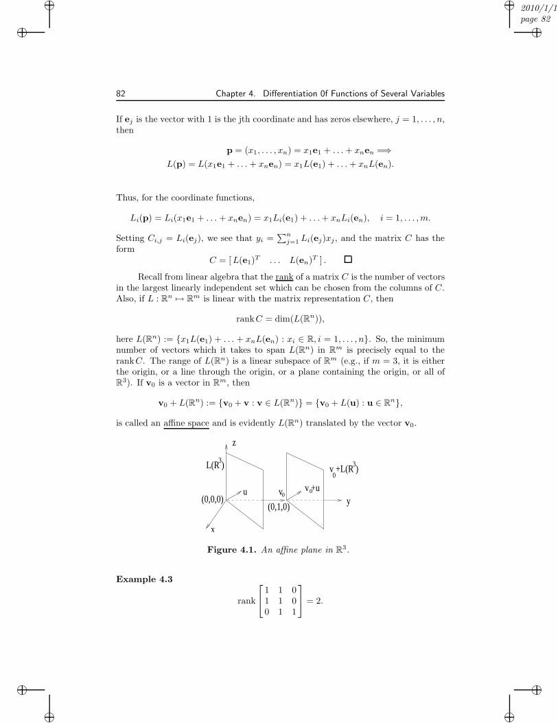
“muldowney”2010/1/10page 82
i
i
i
i
i
i
i
i
82 Chapter 4. Differentiation 0f Functions of Several Variables
If ej is the vector with 1 is the jth coordinate and has zeros elsewhere, j = 1, . . . , n,then
p = (x1, . . . , xn) = x1e1 + . . .+ xnen =⇒L(p) = L(x1e1 + . . .+ xnen) = x1L(e1) + . . .+ xnL(en).
Thus, for the coordinate functions,
Li(p) = Li(x1e1 + . . .+ xnen) = x1Li(e1) + . . .+ xnLi(en), i = 1, . . . ,m.
Setting Ci,j = Li(ej), we see that yi =∑n
j=1 Li(ej)xj , and the matrix C has theform
C = [L(e1)T . . . L(en)
T ] .
Recall from linear algebra that the rank of a matrix C is the number of vectorsin the largest linearly independent set which can be chosen from the columns of C.Also, if L : Rn 7→ Rm is linear with the matrix representation C, then
rankC = dim(L(Rn)),
here L(Rn) := {x1L(e1) + . . . + xnL(en) : xi ∈ R, i = 1, . . . , n}. So, the minimumnumber of vectors which it takes to span L(Rn) in Rm is precisely equal to therankC. The range of L(Rn) is a linear subspace of Rm (e.g., if m = 3, it is eitherthe origin, or a line through the origin, or a plane containing the origin, or all ofR3). If v0 is a vector in Rm, then
v0 + L(Rn) := {v0 + v : v ∈ L(Rn)} = {v0 + L(u) : u ∈ Rn},
is called an affine space and is evidently L(Rn) translated by the vector v0.
z
yv +uu o
L(R )
(0,0,0)(0,1,0)
3v +L(R )0
3
vo
x
Figure 4.1. An affine plane in R3.
Example 4.3
rank
1 1 01 1 00 1 1
= 2.
“muldowney”2010/1/10page 83
i
i
i
i
i
i
i
i
4.1. Preliminaries 83
Thus, for the linear map L : R3 7→ R3 corresponding to this matrix, the rangeL(R3) has dimension 2. In fact, it consists of all vectors of the form (s, s, t), that isthe plane x = y. An example of an affine space in R3 is (0, 1, 0) + L(R3), which isthe parallel plane through the point (0, 1, 0), i.e., the plane y = x+ 1.
Theorem 4.4. If L is linear, there is a constant M such that
|L(p)| ≤M |p|, ∀ p ∈ Rn.
Proof. Using the matrix representation of a linear map, we have by the Cauchy-Schwartz inequality
|yi| = |Li(p)| = |n∑
j=1
Ci,jxj | ≤
√√√√n∑
j=1
C2i,j
√√√√n∑
j=1
x2j
=⇒ |L(p)| =
√√√√m∑
i=1
y2i ≤
√√√√m∑
i=1
n∑
j=1
C2i,j
√√√√n∑
j=1
x2j
or |L(p)| ≤M |p| where M :=
√√√√m∑
i=1
n∑
j=1
C2i,j .
Corollary 4.5. A linear function L : Rn 7→ Rm is uniformly continuous on Rn.
Proof. By the previous theorem
|L(p1)− L(p2)| = |L(p1 − p2)| ≤M |p1 − p2|.
Thus, |p1 − p2| < ǫ/M =⇒ |L(p1)− L(p2)| < ǫ.
Definition 4.6. L : Rn 7→ Rm is one-to-one (1-1) if L(p1) = L(p2) impliesp1 = p2. Equivalently, p1 6= p2 implies L(p1) 6= L(p2).
The next theorem says that for one-to-one linear functions, the inequality inTheorem 4.4 can be reversed!
Theorem 4.7. Suppose L : Rn 7→ Rm is linear. Then L is one-to-one if and onlyif there exists a constant k > 0 such that |L(p)| ≥ k|p| for all p ∈ Rn.
Proof. “⇐=” If such a constant k exists, then
|L(p1)− L(p2)| = |L(p1 − p2)| ≥ k|p1 − p2|.
Thus, p1 6= p2 =⇒ |L(p1) 6= L(p2).
“muldowney”2010/1/10page 84
i
i
i
i
i
i
i
i
84 Chapter 4. Differentiation 0f Functions of Several Variables
“=⇒” L is continuous on Rn by Corollary 4.5, which implies that |L| is con-tinuous on Rn, and in particular, |L| is continuous on S := {p : |p| = 1}. Since S iscompact and |L| is continuous on S, |L| achieves its minimum on S at some point,call it p0. Thus, we define
k := min{|L(p)| : |p| ∈ S} = |L(p0)|, and |p0| = 1.
Since L(O) = 0 by linearity and L is one-to-one, we have k = |L(p0)| > 0 = |L(O)|.Finally, for an arbitrary p ∈ Rn\{O}, p/|p| ∈ S and
k ≤∣∣∣∣L(
1
|p|p)∣∣∣∣ =
1
|p| |L(p)|.
Exercises
4.1. Let L : R2 7→ R3 be linear with L(e1) = (2, 1, 0), L(e2) = (1, 0,−1), wheree1 = (1, 0), e2 = (0, 1). Find L(2, 0), L(1, 1), L(1, 3). Draw pictures.
4.2. Show that L(R2) 6= R3 for the function in the last exercise.
4.3. Show that if L : R2 7→ R3 is linear, then L(R2) 6= R3.
4.4. Let L : R3 7→ R2 be linear. Show that there are non-zero vectors p ∈ R3 suchthat L(p) = O.
4.5. If L : R2 7→ R2 has a matrix
[a bc d
], show that
(i) L(R2) is a point if and only if a = b = c = d = 0.
(ii) L(R2) is a line if and only if ∆ = ad− bc = 0 and a2 + b2 + d2 + c2 > 0.
(iii) L(R2) = R2 if and only if ∆ 6= 0.
4.6. Show that in case (iii) of the last exercise, that L is one-to-one (and only inthat case), and that the inverse function L−1 is linear with matrix
[d∆
−b∆−c
∆a∆
].
4.7. Show that the sum and composition of two linear functions are linear. Whatare the matrix representations of these?
4.8. If L : Rn 7→ Rm is linear and one-to-one, then L−1 is linear on its domain.
4.9. Let f : Rn 7→ Rm be such that
(i) f(p + q) = f(p) + f(q), for all p,q ∈ Rn (additive)
(ii) f is continuous at O.
Prove that f is a linear function.
4.10. Let f : R 7→ Rm be such that
f(λx) = λf(x) (f is homogeneous).
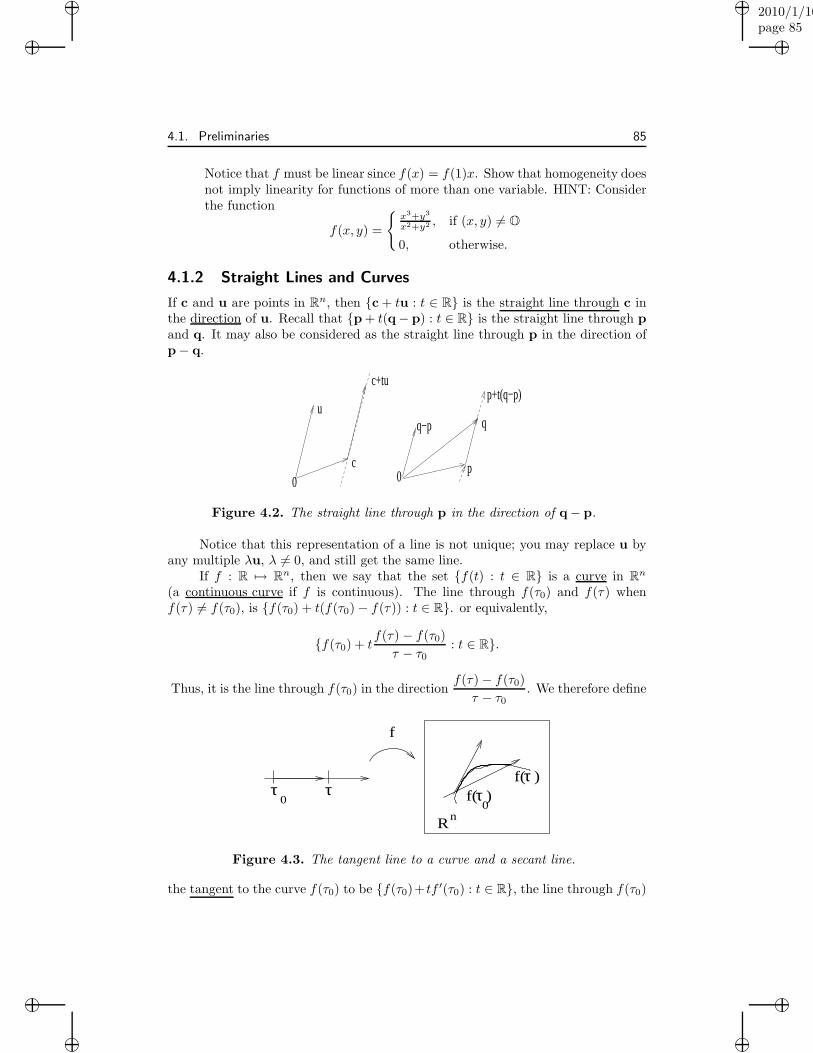
“muldowney”2010/1/10page 85
i
i
i
i
i
i
i
i
4.1. Preliminaries 85
Notice that f must be linear since f(x) = f(1)x. Show that homogeneity doesnot imply linearity for functions of more than one variable. HINT: Considerthe function
f(x, y) =
{x3+y3
x2+y2 , if (x, y) 6= O
0, otherwise.
4.1.2 Straight Lines and Curves
If c and u are points in Rn, then {c + tu : t ∈ R} is the straight line through c inthe direction of u. Recall that {p + t(q− p) : t ∈ R} is the straight line through pand q. It may also be considered as the straight line through p in the direction ofp− q.
0
u
c
c+tu
q
0p
q−p
p+t(q−p)
Figure 4.2. The straight line through p in the direction of q− p.
Notice that this representation of a line is not unique; you may replace u byany multiple λu, λ 6= 0, and still get the same line.
If f : R 7→ Rn, then we say that the set {f(t) : t ∈ R} is a curve in Rn
(a continuous curve if f is continuous). The line through f(τ0) and f(τ) whenf(τ) 6= f(τ0), is {f(τ0) + t(f(τ0)− f(τ)) : t ∈ R}. or equivalently,
{f(τ0) + tf(τ) − f(τ0)
τ − τ0: t ∈ R}.
Thus, it is the line through f(τ0) in the directionf(τ)− f(τ0)
τ − τ0. We therefore define
R
f( )f( )τ
τn
0τ τ
0
f
Figure 4.3. The tangent line to a curve and a secant line.
the tangent to the curve f(τ0) to be {f(τ0)+ tf ′(τ0) : t ∈ R}, the line through f(τ0)
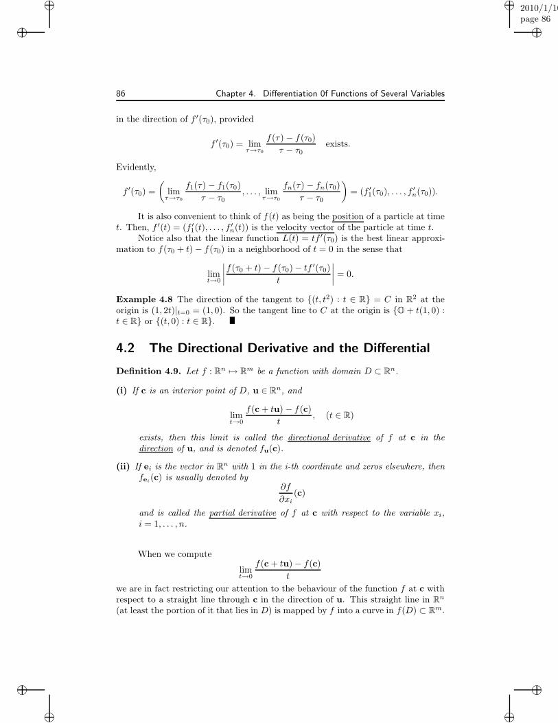
“muldowney”2010/1/10page 86
i
i
i
i
i
i
i
i
86 Chapter 4. Differentiation 0f Functions of Several Variables
in the direction of f ′(τ0), provided
f ′(τ0) = limτ→τ0
f(τ) − f(τ0)
τ − τ0exists.
Evidently,
f ′(τ0) =
(limτ→τ0
f1(τ) − f1(τ0)τ − τ0
, . . . , limτ→τ0
fn(τ)− fn(τ0)τ − τ0
)= (f ′
1(τ0), . . . , f′n(τ0)).
It is also convenient to think of f(t) as being the position of a particle at timet. Then, f ′(t) = (f ′
1(t), . . . , f′n(t)) is the velocity vector of the particle at time t.
Notice also that the linear function L(t) = tf ′(τ0) is the best linear approxi-mation to f(τ0 + t)− f(τ0) in a neighborhood of t = 0 in the sense that
limt→0
∣∣∣∣f(τ0 + t)− f(τ0)− tf ′(τ0)
t
∣∣∣∣ = 0.
Example 4.8 The direction of the tangent to {(t, t2) : t ∈ R} = C in R2 at theorigin is (1, 2t)|t=0 = (1, 0). So the tangent line to C at the origin is {O + t(1, 0) :t ∈ R} or {(t, 0) : t ∈ R}.
4.2 The Directional Derivative and the Differential
Definition 4.9. Let f : Rn 7→ Rm be a function with domain D ⊂ Rn.
(i) If c is an interior point of D, u ∈ Rn, and
limt→0
f(c + tu)− f(c)
t, (t ∈ R)
exists, then this limit is called the directional derivative of f at c in thedirection of u, and is denoted fu(c).
(ii) If ei is the vector in Rn with 1 in the i-th coordinate and zeros elsewhere, thenfei
(c) is usually denoted by∂f
∂xi(c)
and is called the partial derivative of f at c with respect to the variable xi,i = 1, . . . , n.
When we compute
limt→0
f(c + tu)− f(c)
t
we are in fact restricting our attention to the behaviour of the function f at c withrespect to a straight line through c in the direction of u. This straight line in Rn
(at least the portion of it that lies in D) is mapped by f into a curve in f(D) ⊂ Rm.
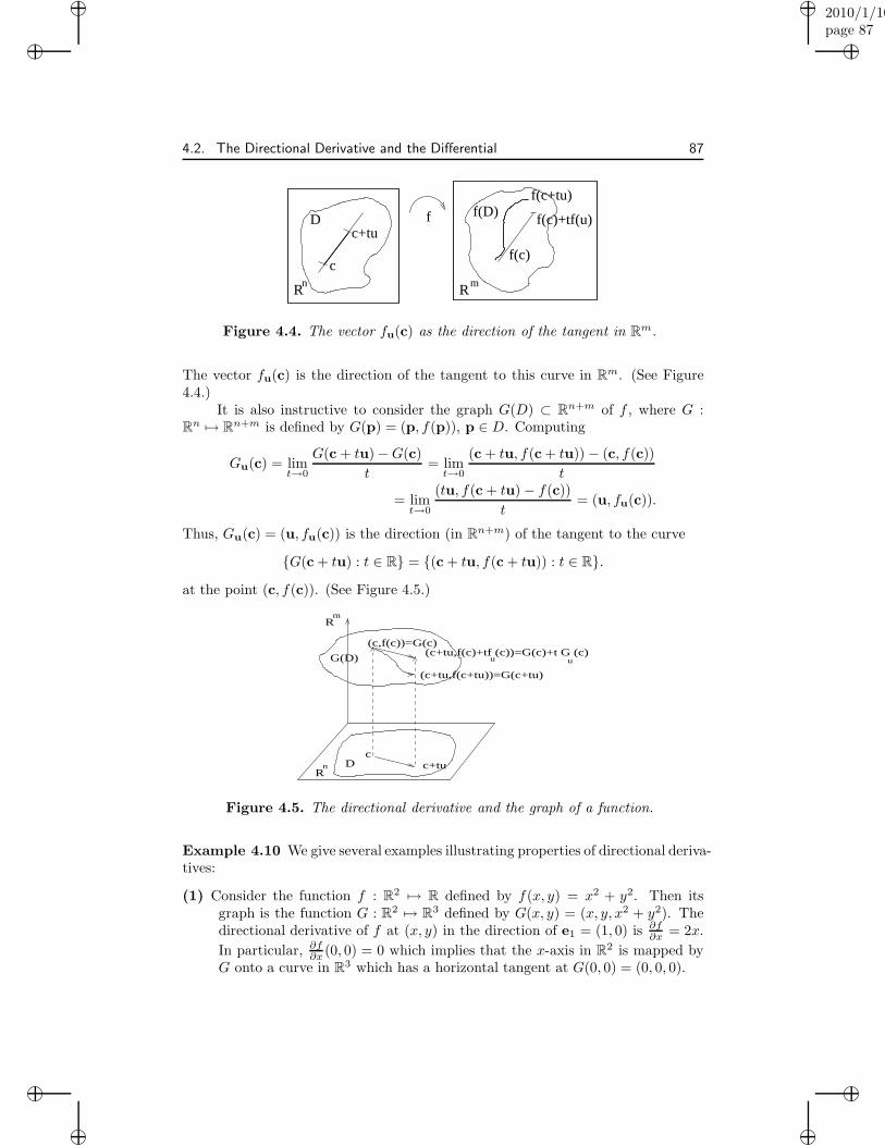
“muldowney”2010/1/10page 87
i
i
i
i
i
i
i
i
4.2. The Directional Derivative and the Differential 87
R
Df(D)
f(c+tu)
f(c)+tf(u)fc+tu
cf(c)
mnR
Figure 4.4. The vector fu(c) as the direction of the tangent in Rm.
The vector fu(c) is the direction of the tangent to this curve in Rm. (See Figure4.4.)
It is also instructive to consider the graph G(D) ⊂ Rn+m of f , where G :Rn 7→ Rn+m is defined by G(p) = (p, f(p)), p ∈ D. Computing
Gu(c) = limt→0
G(c + tu)−G(c)
t= limt→0
(c + tu, f(c + tu))− (c, f(c))
t
= limt→0
(tu, f(c + tu)− f(c))
t= (u, fu(c)).
Thus, Gu(c) = (u, fu(c)) is the direction (in Rn+m) of the tangent to the curve
{G(c + tu) : t ∈ R} = {(c + tu, f(c + tu)) : t ∈ R}.
at the point (c, f(c)). (See Figure 4.5.)
R
R
G(D)
Dc
c+tu
(c+tu,f(c+tu))=G(c+tu)
(c,f(c))=G(c)
n
m
(c+tu,f(c)+tf (c))=G(c)+t G (c)uu
Figure 4.5. The directional derivative and the graph of a function.
Example 4.10 We give several examples illustrating properties of directional deriva-tives:
(1) Consider the function f : R2 7→ R defined by f(x, y) = x2 + y2. Then itsgraph is the function G : R2 7→ R3 defined by G(x, y) = (x, y, x2 + y2). Thedirectional derivative of f at (x, y) in the direction of e1 = (1, 0) is ∂f
∂x = 2x.
In particular, ∂f∂x (0, 0) = 0 which implies that the x-axis in R2 is mapped byG onto a curve in R3 which has a horizontal tangent at G(0, 0) = (0, 0, 0).
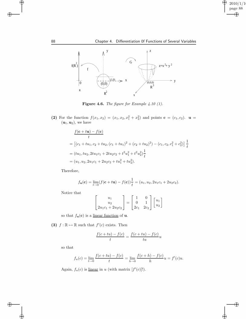
“muldowney”2010/1/10page 88
i
i
i
i
i
i
i
i
88 Chapter 4. Differentiation 0f Functions of Several Variables
f(R )2
0
RR
R
x
y z
x
y
z=x + y f
(0,0)(1,0)
2
3
2 2
(0,0,0)
G
Figure 4.6. The figure for Example 4.10 (1).
(2) For the function f(x1, x2) = (x1, x2, x21 + x2
2) and points c = (c1, c2). u =(u1,u2), we have
f(c + tu)− f(c)
t
=[(c1 + tu1, c2 + tu2, (c1 + tu1)
2 + (c2 + tu2)2)− (c1, c2, c
21 + c22)
] 1
t
= (tu1, tu2, 2tu1c1 + 2tu2c2 + t2u21 + t2u2
2)1
t
= (u1, u2, 2u1c1 + 2u2c2 + tu21 + tu2
2).
Therefore,
fu(c) = limt→0
(f(c + tu)− f(c))1
t= (u1, u2, 2u1c1 + 2u2c2).
Notice that
u1
u2
2u1c1 + 2u2c2
=
1 00 1
2c1 2c2
[u1
u2
]
so that fu(c) is a linear function of u.
(3) f : R 7→ R such that f ′(c) exists. Then
f(c+ tu)− f(c)
t=f(c+ tu)− f(c)
tuu
so that
fu(c) = limt→0
f(c+ tu)− f(c)
t= limh→0
f(c+ h)− f(c)
hu = f ′(c)u.
Again, fu(c) is linear in u (with matrix [f ′(c)]!).
“muldowney”2010/1/10page 89
i
i
i
i
i
i
i
i
4.2. The Directional Derivative and the Differential 89
(4) Now for the bad news. Define f : R2 7→ R by
f(x, y) =
0, when y 6= x2;
1, when y = x2 and (x, y) 6= O;
0, when (x, y) = O.
Then fu(0, 0) = 0 for every u = (u1, u2) ∈ R2 and is linear in u, but f isnot continuous at (0, 0). In other words, the directional derivative exists inevery direction at the origin, but the function is not continuous there. Whathappened to the univariate “differentiable implies continuous”?
(5) This example shows that the directional derivative does not have to be linearin u. Define f : R2 7→ R by
f(x, y) =
{x2yx3−y2 , when x3 6= y2;
0, when x3 = y2.
Then f is not continuous at (0, 0) (why?!). Computing fu(0, 0), for u =(u, v) ∈ R2, we find
f(u,v)(0, 0) =
{−u2
v , if v 6= 0;
0, if v = 0.
In particular, f(u,v) is not linear in u = (u, v).
The preceding examples show that when f is a “nice” function at c, then fu(c)is linear in u, but in general it does not need to be linear even if it exists for all u.Observe however, that all the fu(c) in the above examples are homogeneous in u,that is, fλu(c) = λfu(c) for all λ ∈ R. When they fail to be linear, it is the additiveproperty that fails. The homogeneity in u is always true when fu(c) exists.
Exercises
4.11. Prove that if fu(c) exists, then fλu(c) = λfu(c).
4.12. Prove that the expressions given in the directional derivatives of (4) and (5)in Example 4.10 are correct.
4.13. Check that the following partial derivatives are correct:
(a) The function f(x, y) = x2 + y3 has partial derivatives
∂f
∂x(x, y) = 2x,
∂f
∂y(x, y) = 3y2,
“muldowney”2010/1/10page 90
i
i
i
i
i
i
i
i
90 Chapter 4. Differentiation 0f Functions of Several Variables
(b) The function f(x, y) = (sin(xy), ex, cos(y)) has partial derivatives
∂f
∂x(x, y) = (y cos(xy), ex, 0),
∂f
∂y(x, y) = (x cos(xy), 0,− sin(y)).
4.14. For the function f : R2 7→ R3 defined by f(x, y) = (x2 + y3, sin(y), ex), provethat fu(x, y) exists for each (x, y) ∈ R2 and each direction u = (u, v). Showalso that fu(x, y) is linear in u = (u, v) with matrix
2x 3y2
0 cos(y)ex 0
.
Motivation: At first glance it seems that the directional derivative determines theproperties of functions in the same way that the derivative in one variable does.Unfortunately, that is not quite the case. For example, in Example 4.10 (4), wehave shown that a function may be discontinuous at a point where all directionalderivatives exist. Therefore, a more rigorous approach must be used to extend therole of differentiation. By reforulating the definition, we can realize the “expected”properties, and hence the usefulness, of the derivative. To this end, we reformulatethe definition of the derivative of a function in one variable to show case the linearityas found in Example 4.10 (3).
Definition 4.11 (Derivative in one variable reformulated). A function f :R 7→ R is differentiable at c if there exists a number f ′(c) such that
limx→c
f(x)− f(c)
x− c = f ′(c)
=⇒ limx→c
∣∣∣∣f(x)− f(c)
x− c − f ′(c)
∣∣∣∣ = limx→c
|f(x)− f(c)− f ′(c)(x− c)||x− c| = 0.
Thus, the function f : R 7→ R is differentiable at c if and only if there exists a linearfunction L : R 7→ R such that
limx→c
|f(x)− f(c)− L(x− c)||x− c| = 0 (4.1)
and L is given by L(u) = f ′(c)(u), for all u in R.
We can consider the linear function L to be the best linear approximation inthe sense of (4.1) to f(x)− f(c) in a neighborhood of c, i.e. f(x)− f(c) ≈ L(x− c),or f(x) ≈ L(x − c) + f(c) = f ′(c)(x − c) + f(c). This is the approximation alongthe tangent line (affine function) learned in calculus.
Definition 4.12 (Differential in several variables). Let f : D ⊂ Rn 7→ Rm
with c and interior point of D, the domain of f . Suppose L : Rn 7→ Rm is linearand
limp→c
|f(p)− f(c)− L(p− c)||p− c| = 0.

“muldowney”2010/1/10page 91
i
i
i
i
i
i
i
i
4.2. The Directional Derivative and the Differential 91
c x
(x,f(c)+L(x−c))f(c)
f(x)(x,f(x))
(c,f(c))
Figure 4.7. Derivative as best linear approximation.
Then f is said to be differentiable at c, while L is called the differential of f at cand is denoted Df(c), that is L(u) = Df(c)u, for all u ∈ Rn.
Example 4.13 If f : R 7→ R is given by f(x) = x3, then f ′(c) = 3c2, so L(u) =3c2u for all u ∈ R. Indeed, computing
|f(p)− f(c)− L(p− c)| = |p3 − c3 − 3c2(p− c)| = |p− c||p2 + pc+ c2 − 3c2|= |p− c||p2 + pc− 2c2|
=⇒ limp→c
|f(p)− f(c)− L(p− c)||p− c| = lim
p→c|p2 + pc− 2c2| = 0.
Theorem 4.14. For a function f : D ⊂ Rn 7→ Rm and a point c interior to D, wehave
Df(c)(u) = L(u)⇐⇒ Dfi(c) = Li(u), ∀u ∈ Rn and i = 1, . . . ,m,
wheref(p) = (f1(p), . . . , fm(p)), L(u) = (L1(u), . . . , Lm(u)).
Proof. This follows because the limit exists if and only if the limit of each compo-nent exists (this uses the equivalence of d(p, c) and d∞(p, c)):
limp→c
|f(p)− f(c)− L(p− c)||p− c| = 0
⇐⇒ limp→c
|fi(p)− fi(c) − Li(p− c)||p− c| = 0, i = 1, . . . ,m
The matrix for the differential must have the form provided by the next the-orem.
Theorem 4.15. If f : D ⊂ Rn 7→ Rm and f is differentiable at an interior pointc of D, then
“muldowney”2010/1/10page 92
i
i
i
i
i
i
i
i
92 Chapter 4. Differentiation 0f Functions of Several Variables
(i) fu(c) exists for each u ∈ Rn and Df(c)(u) = fu(c).
(ii) The matrix of the linear transformation Df(c) is
∂f1∂x1
(c) . . . ∂f1∂xn
(c)
... . . ....
∂fm
∂x1(c) . . . ∂fm
∂xn(c)
,
This matrix is the Jacobian Matrix of f at c, and can be denoted also as[∂f∂x (c)
], or simply f ′(c).
Proof. (i) If Df(c) exists, then for u ∈ Rn\O and p = c + tu,
limt→0
|f(c + tu)− f(c)−Df(c)(tu)||tu| = 0
=⇒ 1
|u| limt→0
∣∣∣∣f(c + tu)− f(c)
t−Df(c)(u)
∣∣∣∣ = 0
=⇒ limt→0
f(c + tu)− f(c)
t= Df(c)(u).
Here we used the homogeneous property of linearity, Df(c)(tu) = tDf(c)(u) forthe second step.
(ii) recall from Theorem 4.2 that the matrix of L is [Ci,j ] = [Li(ej)]. Here
Li(ej) = Dfi(c)(ej) = (fi)ej(c) by part (i)
=∂fi∂xj
(c), i = 1, . . . ,m, j = 1, . . . , n.
Notes: In the case when n = m, the determinant det f ′(c) is called the Jacobianof f at c and is often denoted by
Jf (c) or∂(f1, . . . , fn)
∂(x1, . . . , xn)(c).
Part (ii) of the Theorem means that if u = (u1, . . . , un) ∈ Rn, then for i = 1, . . . ,m,
Li(u) = Dfi(c)(u) =
n∑
j=1
∂fi∂xj
(c)uj .
Corollary 4.16. If the differential exists, it is unique.
Proof. fu(c) is unique (from the uniqueness of limits) for each u ∈ Rn. Alter-
natively, the partials ∂fi
∂xj(c) are unique and hence the matrix f ′(c) =
[∂fi
∂xj(c)]
is
unique.
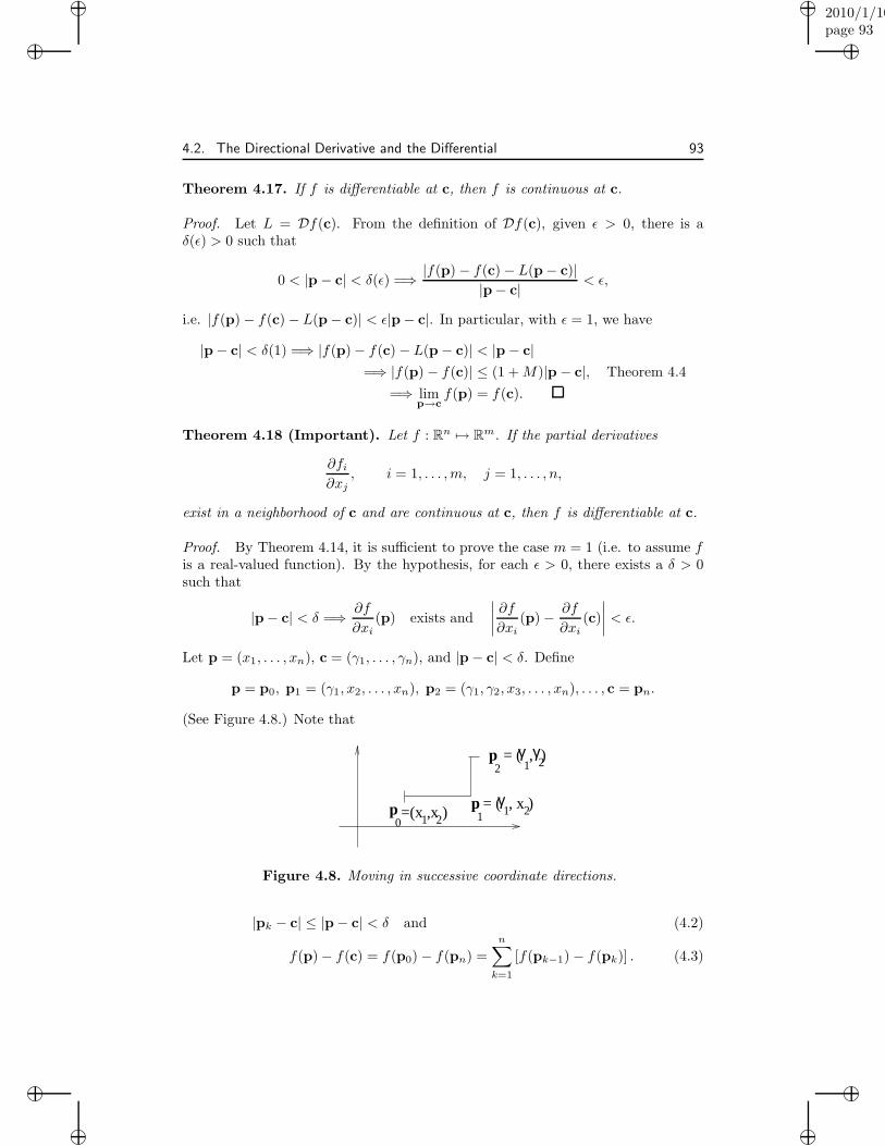
“muldowney”2010/1/10page 93
i
i
i
i
i
i
i
i
4.2. The Directional Derivative and the Differential 93
Theorem 4.17. If f is differentiable at c, then f is continuous at c.
Proof. Let L = Df(c). From the definition of Df(c), given ǫ > 0, there is aδ(ǫ) > 0 such that
0 < |p− c| < δ(ǫ) =⇒ |f(p)− f(c)− L(p− c)||p− c| < ǫ,
i.e. |f(p)− f(c)− L(p− c)| < ǫ|p− c|. In particular, with ǫ = 1, we have
|p− c| < δ(1) =⇒ |f(p)− f(c)− L(p− c)| < |p− c|=⇒ |f(p)− f(c)| ≤ (1 +M)|p− c|, Theorem 4.4
=⇒ limp→c
f(p) = f(c).
Theorem 4.18 (Important). Let f : Rn 7→ Rm. If the partial derivatives
∂fi∂xj
, i = 1, . . . ,m, j = 1, . . . , n,
exist in a neighborhood of c and are continuous at c, then f is differentiable at c.
Proof. By Theorem 4.14, it is sufficient to prove the case m = 1 (i.e. to assume fis a real-valued function). By the hypothesis, for each ǫ > 0, there exists a δ > 0such that
|p− c| < δ =⇒ ∂f
∂xi(p) exists and
∣∣∣∣∂f
∂xi(p)− ∂f
∂xi(c)
∣∣∣∣ < ǫ.
Let p = (x1, . . . , xn), c = (γ1, . . . , γn), and |p− c| < δ. Define
p = p0, p1 = (γ1, x2, . . . , xn), p2 = (γ1, γ2, x3, . . . , xn), . . . , c = pn.
(See Figure 4.8.) Note that
p
p
=(x ,x )p = ( , x )
= ( , )
γ
γ γ
11
1
122
22
0
Figure 4.8. Moving in successive coordinate directions.
|pk − c| ≤ |p− c| < δ and (4.2)
f(p)− f(c) = f(p0)− f(pn) =
n∑
k=1
[f(pk−1)− f(pk)] . (4.3)
“muldowney”2010/1/10page 94
i
i
i
i
i
i
i
i
94 Chapter 4. Differentiation 0f Functions of Several Variables
Now on each line segment between pk−1 and pk, k = 1, . . . , n, we are really consid-ering a real-valued differentiable function of a real variable so we may use the MeanValue Theorem.
f(pk−1)− f(pk) =∂f
∂xk(p∗k)(xk − γk) (4.4)
where p∗k is on the line segment from pk−1 to pk, k = 1, . . . , n. Clearly, p∗
k ∈ {p :|p− c| < δ} by (4.2), since this set is convex. From (4.3) and (4.2), we find
f(p)− f(c) =n∑
k=1
∂f
∂xk(p∗k)(xk − γk).
If u = (u1, . . . , un), let L(u) be defined by
L(u) =
n∑
k=1
∂f
∂xk(c)uk.
Then since |pk − c| < δ when |p− c| < δ, we have
∣∣f(p)− f(c)− L(p− c)∣∣ =
∣∣∣∑n
k=1
[∂f∂xk
(p∗k)− ∂f
∂xk(c)](xk − γk)
∣∣∣
≤[∑n
k=1
(∂f∂xk
(p∗k)− ∂f
∂xk(c))2]1/2 [
[∑n
k=1(xk − γk)2]1/2
(Cauchy-Schwartz)
≤ √nǫ|p− c|
=⇒ |f(p)−f(c)−L(p−c)||p−c| <
√n ǫ, when |p− c| < δ
Therefore, Df(c) exists and Df(c) = L.
Please note that the last Theorem gives only a sufficient condition for thefunction to be differentiable at a point.
Example 4.19 Let f : R2 7→ R3 be given by f(x1, x2) = (x1, x2, x21 + x2
2). Thepartial derivatives are continuous on R2 so f is differentiable and Df(x1, x2) hasthe matrix representation
f ′(x1, x2) =
1 00 1
2x1 2x2
.
For example, if L = Df(0, 0), then L : R2 7→ R3 and
L1uL2uL3u
=
1 00 10 0
[u1
u2
], where u = (u1, u2).
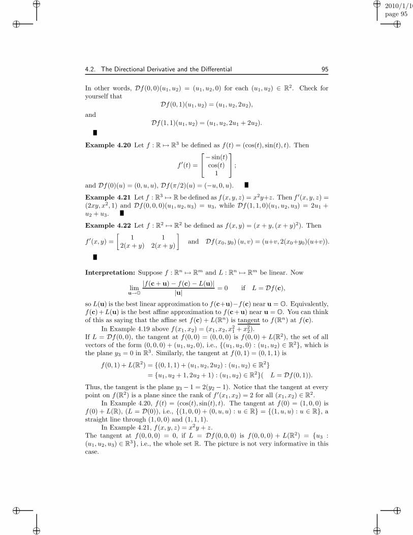
“muldowney”2010/1/10page 95
i
i
i
i
i
i
i
i
4.2. The Directional Derivative and the Differential 95
In other words, Df(0, 0)(u1, u2) = (u1, u2, 0) for each (u1, u2) ∈ R2. Check foryourself that
Df(0, 1)(u1, u2) = (u1, u2, 2u2),
andDf(1, 1)(u1, u2) = (u1, u2, 2u1 + 2u2).
Example 4.20 Let f : R 7→ R3 be defined as f(t) = (cos(t), sin(t), t). Then
f ′(t) =
− sin(t)cos(t)
1
;
and Df(0)(u) = (0, u, u), Df(π/2)(u) = (−u, 0, u).Example 4.21 Let f : R3 7→ R be defined as f(x, y, z) = x2y+z. Then f ′(x, y, z) =(2xy, x2, 1) and Df(0, 0, 0)(u1, u2, u3) = u3, while Df(1, 1, 0)(u1, u2, u3) = 2u1 +u2 + u3.
Example 4.22 Let f : R2 7→ R2 be defined as f(x, y) = (x+ y, (x+ y)2). Then
f ′(x, y) =
[1 1
2(x+ y) 2(x+ y)
]and Df(x0, y0) (u, v) = (u+v, 2(x0+y0)(u+v)).
Interpretation: Suppose f : Rn 7→ Rm and L : Rn 7→ Rm be linear. Now
limu→O
|f(c + u)− f(c)− L(u)||u| = 0 if L = Df(c),
so L(u) is the best linear approximation to f(c+u)−f(c) near u = O. Equivalently,f(c)+L(u) is the best affine approximation to f(c+u) near u = O. You can thinkof this as saying that the affine set f(c) + L(Rn) is tangent to f(Rn) at f(c).
In Example 4.19 above f(x1, x2) = (x1, x2, x21 + x2
2).If L = Df(0, 0), the tangent at f(0, 0) = (0, 0, 0) is f(0, 0) + L(R2), the set of allvectors of the form (0, 0, 0) + (u1, u2, 0), i.e., {(u1, u2, 0) : (u1, u2) ∈ R2}, which isthe plane y3 = 0 in R3. Similarly, the tangent at f(0, 1) = (0, 1, 1) is
f(0, 1) + L(R2) = {(0, 1, 1) + (u1, u2, 2u2) : (u1, u2) ∈ R2}= {u1, u2 + 1, 2u2 + 1) : (u1, u2) ∈ R2}( L = Df(0, 1)).
Thus, the tangent is the plane y3 − 1 = 2(y2 − 1). Notice that the tangent at everypoint on f(R2) is a plane since the rank of f ′(x1, x2) = 2 for all (x1, x2) ∈ R2.
In Example 4.20, f(t) = (cos(t), sin(t), t). The tangent at f(0) = (1, 0, 0) isf(0) + L(R), (L = D(0)), i.e., {(1, 0, 0) + (0, u, u) : u ∈ R} = {(1, u, u) : u ∈ R}, astraight line through (1, 0, 0) and (1, 1, 1).
In Example 4.21, f(x, y, z) = x2y + z.The tangent at f(0, 0, 0) = 0, if L = Df(0, 0, 0) is f(0, 0, 0) + L(R2) = {u3 :(u1, u2, u3) ∈ R3}, i.e., the whole set R. The picture is not very informative in thiscase.
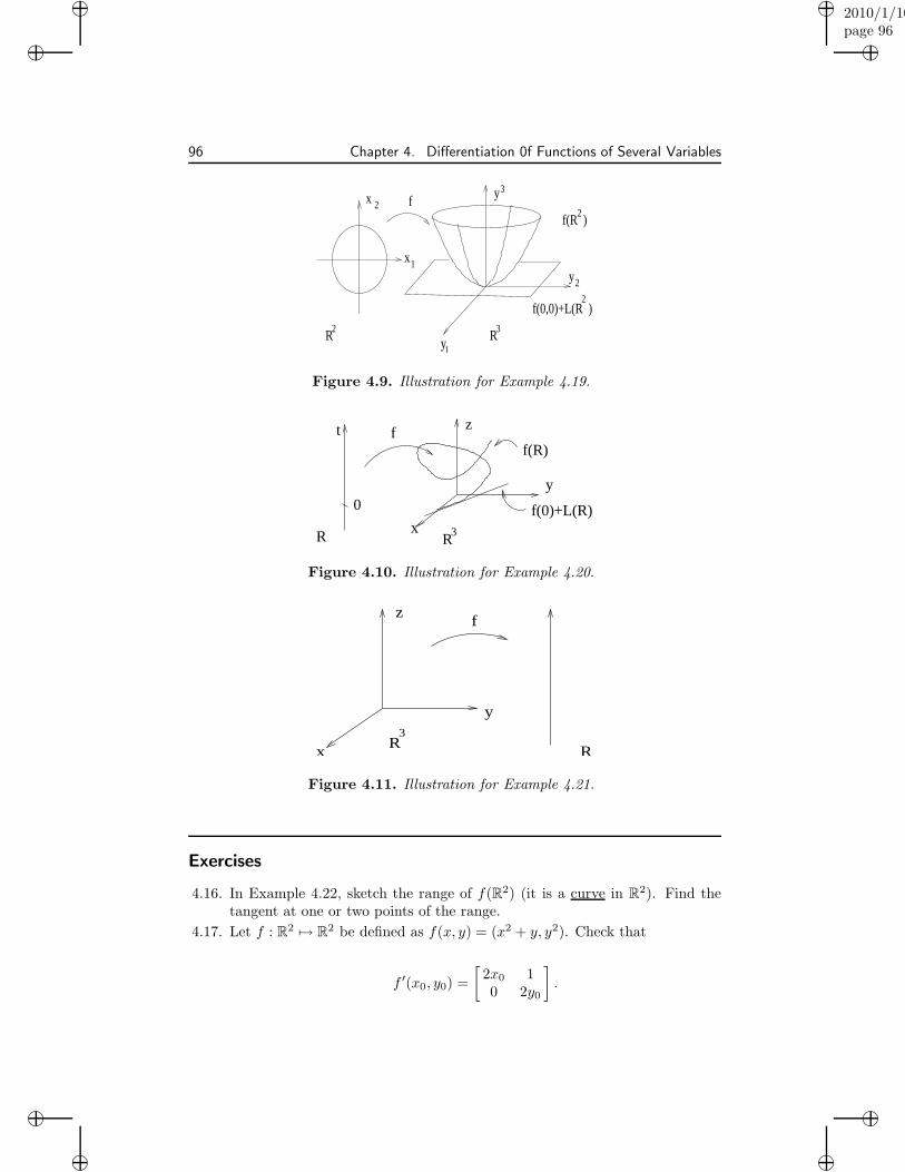
“muldowney”2010/1/10page 96
i
i
i
i
i
i
i
i
96 Chapter 4. Differentiation 0f Functions of Several Variables
R Ry
y
f(R )
f(0,0)+L(R )
x
x
1
1
2
2
y2
22
3
3f
Figure 4.9. Illustration for Example 4.19.
f(0)+L(R)
R
0
t
x
y
z
f(R)f
3R
Figure 4.10. Illustration for Example 4.20.
x
y
z
RR
f
3
Figure 4.11. Illustration for Example 4.21.
Exercises
4.16. In Example 4.22, sketch the range of f(R2) (it is a curve in R2). Find thetangent at one or two points of the range.
4.17. Let f : R2 7→ R2 be defined as f(x, y) = (x2 + y, y2). Check that
f ′(x0, y0) =
[2x0 10 2y0
].
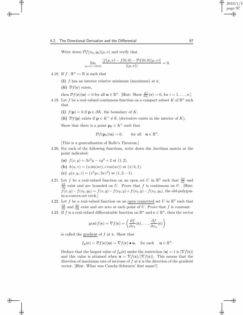
“muldowney”2010/1/10page 97
i
i
i
i
i
i
i
i
4.2. The Directional Derivative and the Differential 97
Write down Df(x0, y0)(µ, ν) and verify that
lim(µ,ν)→(0,0)
|f(µ, ν)− f(0, 0)−Df(0, 0)(µ, ν)||(µ, ν)| = 0.
4.18. If f : Rn 7→ R is such that
(i) f has an interior relative minimum (maximum) at c,
(ii) Df(c) exists,
then Df(c)(u) = 0 for all u ∈ Rn. [Hint: Show ∂f∂xi
(c) = 0, for i = 1, . . . , n.]
4.19. Let f be a real-valued continuous function on a compact subset K of Rn suchthat
(i) f(p) = 0 if p ∈ ∂K, the boundary of K,
(ii) Df(p) exists if p ∈ K◦ 6= ∅, (derivative exists in the interior of K),
Show that there is a point p0 ∈ K◦ such that
Df(p0)(u) = 0, for all u ∈ Rn.
[This is a generalization of Rolle’s Theorem.]
4.20. For each of the following functions, write down the Jacobian matrix at thepoint indicated:
(a) f(x, y) = 3x2y − xy3 + 2 at (1, 2).
(b) h(u, v) = (u sin(uv), v cos(uv)) at (π/4, 1).
(c) g(x, y, z) = (x2yz, 3xz2) at (1, 2,−1).
4.21. Let f be a real-valued function on an open set U in R2 such that ∂f∂x and
∂f∂y exist and are bounded on U . Prove that f is continuous on U . [Hint:
f(x, y)−f(x0, y0) = f(x, y)−f(x0, y)+f(x0, y)−f(x0, y0), the old-polygon-in-a-convex-set trick.]
4.22. Let f be a real-valued function on an open connected set U in R2 such that∂f∂x and ∂f
∂y exist and are zero at each point of U . Prove that f is constant.
4.23. If f is a real-valued differentiable function on Rn and c ∈ Rn, then the vector
gradf(c) = ∇f(c) =
(∂f
∂x1(c), . . . ,
∂f
∂xn(c)
)
is called the gradient of f at c. Show that
fu(c) = Df(c)(u) = ∇f(c) • u, for each u ∈ Rn.
Deduce that the largest value of fu(c) under the restriction |u| = 1 is |∇f(c)|and this value is attained when u = ∇f(c)/|∇f(c)|. This means that thedirection of maximum rate of increase of f at c is the direction of the gradientvector. [Hint: What was Cauchy-Schwartz’ first name?]
“muldowney”2010/1/10page 98
i
i
i
i
i
i
i
i
98 Chapter 4. Differentiation 0f Functions of Several Variables
4.24. Sketch the surface {(x, y, xy) : (x, y) ∈ R2} in R3 (i.e. z = xy) and show thatthe tangent to this surface at the point (1, 1, 1) is (1, 1, 1) + {(u, v, u + v) :(u, v) ∈ R2} (i.e. z + 1 = x+ y).
4.25. If L : Rn 7→ Rm is linear, then the differential L exists and equals L at eachpoint in Rn.
4.2.1 Differentiation Rules
Theorem 4.23. Let φ, ψ be functions from Rn to Rm which are differentiable atc ∈ Rn.
(i) If h = αφ+ βψ, α, β ∈ R, then h is differentiable at c and
Dh(c)(u) = αDφ(c)(u) + βDψ(c)(u), for each u ∈ Rn.
(ii) If k = φ • ψ = 〈φ, ψ〉 (so k : Rn 7→ R), then k is differentiable at c and
Dk(c)(u) = φ(c) • Dψ(c)(u) + ψ(c) • Dφ(c)(u), for each u ∈ Rn.
Proof. (i) Let Lφ = Dφ(c), Lψ = Dψ(c), and consider the function L : Rn 7→ Rm
defined as L(u) = αLφ(u) + βLψ(u). Clearly, L is linear and
|h(p)− h(c)− L(p− c)||p− c|
=|αφ(p) + βψ(p)− αφ(c) − βψ(c) − αLφ(p− c)− βLψ(p− c)|
|p− c|
≤ |α| |αφ(p) − αφ(c) − αLφ(p− c)||p− c| + |β| |ψ(p)− ψ(c) − Lψ(p− c)|
|p− c| ,
by the triangle inequality. Both terms in this last expression have a limit of zero asp→ c, therefore, Dh(c) exists and equals the specified L.
(ii) Let L : Rn → R be defined by
L(u) = φ(c) • Lψ(u) + ψ(c) • Lφ(u), u ∈ Rn.
Then
|k(p)− k(c)− L(p− c)||p− c| =
|φ(p) • ψ(p)− φ(c) • ψ(c)− φ(c) • Lψ(p− c) − ψ(c) • Lφ(p− c)||p− c|
=(|φ(p) • [ψ(p)− ψ(c)− Lψ(p− c)] + ψ(c) • [φ(p)− φ(c) − Lφ(p− c)]
+ [φ(p)− φ(c)] • Lψ(p− c)|)/|p− c|
≤ |φ(p)| |ψ(p) − ψ(c) − Lψ(p− c)||p− c| + |ψ(p)| |φ(p) − φ(c) − Lφ(p− c)|
|p− c|
+ |φ(p) − φ(c)| |Lψ(p− c)||p− c| .
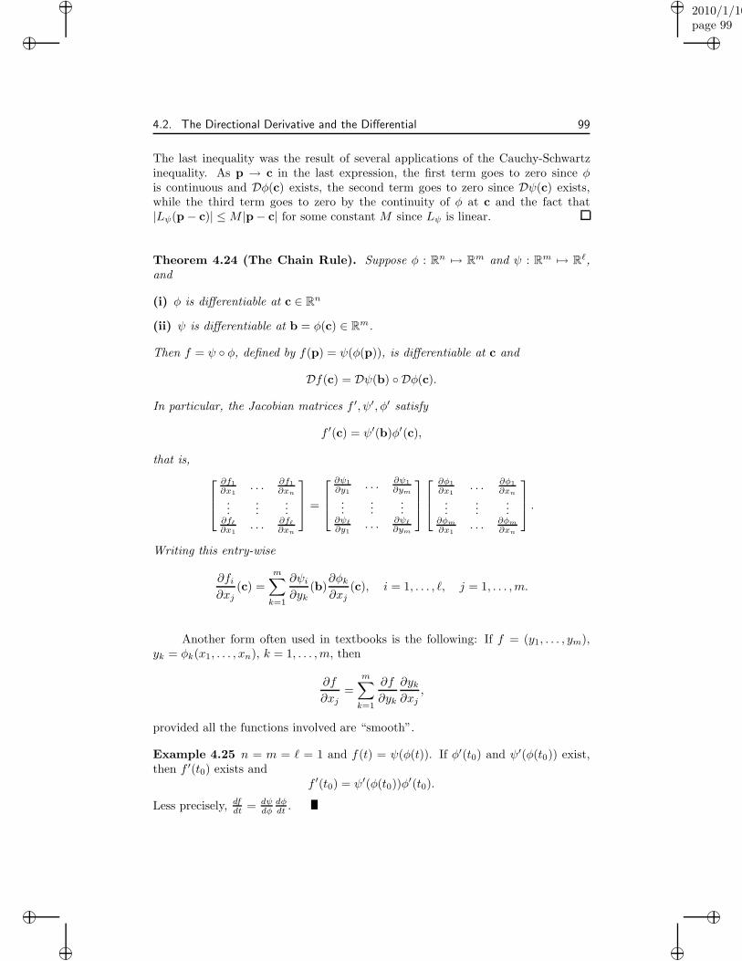
“muldowney”2010/1/10page 99
i
i
i
i
i
i
i
i
4.2. The Directional Derivative and the Differential 99
The last inequality was the result of several applications of the Cauchy-Schwartzinequality. As p → c in the last expression, the first term goes to zero since φis continuous and Dφ(c) exists, the second term goes to zero since Dψ(c) exists,while the third term goes to zero by the continuity of φ at c and the fact that|Lψ(p− c)| ≤M |p− c| for some constant M since Lψ is linear.
Theorem 4.24 (The Chain Rule). Suppose φ : Rn 7→ Rm and ψ : Rm 7→ Rℓ,and
(i) φ is differentiable at c ∈ Rn
(ii) ψ is differentiable at b = φ(c) ∈ Rm.
Then f = ψ ◦ φ, defined by f(p) = ψ(φ(p)), is differentiable at c and
Df(c) = Dψ(b) ◦ Dφ(c).
In particular, the Jacobian matrices f ′, ψ′, φ′ satisfy
f ′(c) = ψ′(b)φ′(c),
that is,
∂f1∂x1
. . . ∂f1∂xn
......
...∂fℓ
∂x1. . . ∂fℓ
∂xn
=
∂ψ1
∂y1. . . ∂ψ1
∂ym
......
...∂ψℓ
∂y1. . . ∂ψℓ
∂ym
∂φ1
∂x1. . . ∂φ1
∂xn
......
...∂φm
∂x1. . . ∂φm
∂xn
.
Writing this entry-wise
∂fi∂xj
(c) =
m∑
k=1
∂ψi∂yk
(b)∂φk∂xj
(c), i = 1, . . . , ℓ, j = 1, . . . ,m.
Another form often used in textbooks is the following: If f = (y1, . . . , ym),yk = φk(x1, . . . , xn), k = 1, . . . ,m, then
∂f
∂xj=
m∑
k=1
∂f
∂yk
∂yk∂xj
,
provided all the functions involved are “smooth”.
Example 4.25 n = m = ℓ = 1 and f(t) = ψ(φ(t)). If φ′(t0) and ψ′(φ(t0)) exist,then f ′(t0) exists and
f ′(t0) = ψ′(φ(t0))φ′(t0).
Less precisely, dfdt = dψdφ
dφdt .
“muldowney”2010/1/10page 100
i
i
i
i
i
i
i
i
100 Chapter 4. Differentiation 0f Functions of Several Variables
Example 4.26 n = m = 2, ℓ = 1. Write
f(x, y) = ψ(u, v), where u = u(x, y), v = v(x, y).
In other words, f = ψ ◦ φ where φ(x, y) = (u(x, y), v(x, y)) If Dφ(x0, y0) andDψ(u0, v0) exist, where u0 = u(x0, y0) and v0 = v(x0, y0), then Df(x0, y0) existsand
f ′(x0, y0) = ψ′(u0, v0)φ′(x0, y0).
In matrix form
[ ∂f∂x
∂f∂y
](x0,y0)
= [ ∂ψ∂u∂φ∂v ](u0,v0)
[ ∂u∂x
∂u∂y
∂v∂x
∂v∂y
]
(x0,y0)
.
Less precisely,
∂f
∂x=∂ψ
∂u
∂u
∂x+∂φ
∂v
∂v
∂x,
∂f
∂y=∂ψ
∂u
∂u
∂y+∂φ
∂v
∂v
∂y.
As a particular example, if h(r, θ) = g(u, v) where u = r cos(θ) and v = r sin(θ),then
∂h
∂r=∂g
∂ucos(θ) +
∂g
∂vsin(θ),
∂h
∂θ=∂g
∂u(−r sin(θ)) +
∂g
∂vr cos(θ).
Example 4.27 n = 1,m = 2, ℓ = 1, F (t) = h(x, y) where x = r(t), y = s(t). Then[dF
dt
]=[ ∂h∂x
∂h∂y
] [ dxdtdydt
],
or,dF
dt=∂h
∂x
dx
dt+∂h
∂y
dy
dt.
Example 4.28 Suppose a particle’s position (x, y, z) in space is given at time t byx = cos(t), y = sin(t), z = t (it is moving on a helix), and the temperature at anypoint (x, y, z) is given by T (x, y, z) = x2 + y2 + z2. If H(t) is the temperature ofthe particle at time t, find ∂H/dt.
In this case, H = T ◦ f , where
T (x, y, z) = x2 + y2 + z2, f(t) = (cos(t), sin(t), t).
From the Chain Rule, H ′(t) = T ′(x, y, z)f ′(t); more exactly
[dH
dt
]= [ 2x 2y 2z ]
− sin(t)cos(t)
1
, ordH
dt= −2x sin(t) + 2y cos(t) + 2z = 2t,
In fact for this case, it is easier to find dHdt directly
H(t) = T (x, y, z) = x2 + y2 + z2 = cos2(t) + sin2(t) + t2 = 1 + t2,
so dH/dt = 2t.
“muldowney”2010/1/10page 101
i
i
i
i
i
i
i
i
4.2. The Directional Derivative and the Differential 101
Proof of Theorem 4.24. Let Lφ = Dφ(c), Lψ = Dψ(c) and b = φ(c). We maketwo assertions
1. limp→c |ψ(φ(p)) − ψ(φ(c)) − Lψ(φ(p) − φ(c))|/|p− c| = 0.
2. limp→c |Lψ(φ(p) − φ(c) − Lφ(p− c))|/|p− c| = 0.
Assuming these, if f = ψ ◦ φ, then
|f(p)− f(c)− Lψ ◦ Lφ(p− c)||p− c|
=|ψ(φ(p)) − ψ(φ(c)) − Lψ(φ(p) − φ(c)) + Lψ(φ(p) − φ(c) − Lφ(p− c))|
|p− c|
≤ |ψ(φ(p)) − ψ(φ(c)) − Lψ(φ(p) − φ(c))||p− c| +
|Lψ(φ(p)− φ(c) − Lφ(p− c))||p− c| → 0
as p → c by (1) and (2). Since Lψ ◦ Lφ is a linear function, we have shown thatDf(c) exists and equals Lψ ◦ Lφ.
It remains to prove assertions (1) and (2). For assertion (1), let ǫ > 0 be given.Since φ is differentiable at c, there is a neighborhood U of c and a constant K > 0such that if p ∈ U , then
|φ(p) − φ(c)| < K|p− c|(see the proof of Theorem 4.17). Since Lψ is the differential of ψ at b = φ(c), thereexists a δ > 0 such that
|q− b| < δ =⇒ |ψ(q) − ψ(b)− Lψ(q− b)| < ǫ
K|q− b|.
Thus, from these two inequalities, if p is sufficiently close to c, we have
|ψ(φ(p)) − ψ(φ(c)) − Lψ(φ(p) − φ(c))| < ǫ
K|φ(p) − φ(c)|< ǫ|p− c|.
Therefore, assertion (1) is proved.For the proof of assertion (2), from the linearity of Lψ, there is a constant
M > 0 such that |Lψ(u)| ≤M |u|, for all u ∈ Rn. Thus,
|Lψ(φ(p) − φ(c) − Lφ(p− c))||p− c| ≤M |φ(p) − φ(c) − Lφ(p− c)|
|p− c| → 0
as p→ c by definition of Lφ.
The Chain Rule in higher dimensions is more interesting than in one dimen-sion; for example, it includes the rules for differentiating sums and products asspecial cases. Thus, Theorem 4.23 is a corollary to Theorem 4.24. This can be seenby considering the functions
F : Rn 7→ R2m, F (p) = (φ(p), ψ(p))
G : R2m 7→ Rm,G(q1,q2) = αq1 + βq2, q1,q2 ∈ Rm
H : R2m 7→ R, H(q1,q2) = q1 • q2.
“muldowney”2010/1/10page 102
i
i
i
i
i
i
i
i
102 Chapter 4. Differentiation 0f Functions of Several Variables
Then G ◦ F = αφ+ βψ and H ◦ F = φ • ψ.
Theorem 4.29 (Mean Value Theorem). Suppose f : Rn 7→ R. If a,b ∈ Rn
and f is differentiable at each point of the line segment S between a and b, thenthere is a point c ∈ S, c 6= a or b, such that
f(b)− f(a) = Df(c)(b − a).
In the notation of Exercise 23, this may be written as
f(b)− f(a) = ∇f(c) • (b− a)
=
n∑
j=1
∂f
∂xj(c)(bj − aj),
where b = (b1, . . . , bn) and a = (a1, . . . , an).
Proof. We reduce the problem to one variable by introducing the function F :[0, 1] 7→ R defined by
F (t) = f(a + t(b− a)), 0 ≤ t ≤ 1
= f(λ(t)), λ(t) = a + t(b− a).
By the Chain Rule, F ′(t) exists for 0 ≤ t ≤ 1 and
F ′(t) = DF (t)(1) = Df(λ(t)) ◦ Dλ(t)(1)
= Df(λ(t))λ′(t) = Df(λ(t))(b − a).
By the Mean Value Theorem for F (t),
F (1)− F (0) = F ′(t0)(1 − 0) = F ′(t0),
for some t0 ∈ (0, 1). Thus,
f(b)− f(a) = Df(λ(t0))(b − a) = Df(c)(b − a), c = λ(t0).
The Mean Value Theorem does not hold for functions f : Rn 7→ Rm if m > 1.Can you tell why? If you cannot, try to carry out a proof with m > 1. See Exercise30 for what can be said.
Exercises
4.26. Let f : R 7→ R be differentiable. If F : R2 7→ R is defined by
(a) F (x, y) = f(xy), then x∂F∂x = y ∂F∂y ,
(b) F (x, y) = f(ax+ by), then b∂F∂x = a∂F∂y ,
“muldowney”2010/1/10page 103
i
i
i
i
i
i
i
i
4.2. The Directional Derivative and the Differential 103
(c) F (x, y) = f(x2 + y2), then y ∂F∂x = x∂F∂y .
4.27. Define f : R2 7→ R by
f(x, y) =
(x2 + y2) sin(
1x2+y2
), if (x, y) 6= (0, 0)
0, if (x, y) = (0, 0).
Show that f is differentiable at (0, 0), but ∂f∂x and ∂f
∂y are not continuous at
(0, 0).
4.28. Let f : Rn 7→ R be a differentiable function and C be a smooth curve inRn on which the function is constant. Prove that for any point c ∈ C, thetangent to C at c is perpendicular to
∇f(c) =
(∂f
∂x1(c), . . . ,
∂f
∂xn(c)
).
4.29. Suppose f : Rn 7→ Rn is differentiable. If for all collections of n Co-linearpoints {p1, . . . ,pn} in Rn the determinant
∣∣∣∣∣∣∣
∂f1∂x1
(p1) . . . ∂f1∂xn
(p1)
......
...∂fn
∂x1(pn) . . . ∂fn
∂xn(pn)
∣∣∣∣∣∣∣
is non-zero, then show that f is 1-to-1 on Rn. Thus, if n = 1 and f ′(x) 6= 0for each x ∈ R, then f is 1-to-1 on R. Show that the function f(x, y) =(x3 − y, ex+y) is 1-to-1 on R2.
4.30. If f : Rn 7→ Rm is differentiable at each point c in the line segment between aand b and satisfies |Df(c)(u)| ≤M |u|, for each u ∈ Rn, then |f(b)−f(a)| ≤M |b− a|.
4.31. (Euler’s Theorem) The real-valued function f(x) = f(x1, . . . , xn) is homogeneousof degree m if
f(tx) = f(tx1, . . . , txn) = tmf(x1, . . . , xn) = tmf(x), ∀ t ∈ R.
For example the functions
x3 + y3 + 3x2y,x5 + y5 + z5
(x + y + z)5, x2y7 + 2z4x5,
are homogeneous of degree 3, 0, 9 respectively. Prove that if f is differentiableand homogeneous of degree m, then
x • ∇f = x1∂f
∂x1+ . . .+ xn
∂f
∂xn= mf.
[Hint: Differentiate the formula defining the concept of homogeneity withrespect to t and set t = 1. Was Euler an Edmonton hockey player???]
“muldowney”2010/1/10page 104
i
i
i
i
i
i
i
i
104 Chapter 4. Differentiation 0f Functions of Several Variables
4.32. (Project) Carry out the following:
(i) Suppose f is continuous on [a, b]× [c, d] = I to R. Prove that if
F (x) =
∫ d
c
f(x, y) dy,
then F is continuous on [a, b]. [Hint: f is uniformly contiguous on I.]
(ii) Suppose f and ∂f∂x are continuous on I. Let F be as in part (i). Prove
that F ′ exists, is continuous on [a, b], and
F ′(x) =
∫ d
c
∂f
∂x(x, y) dy.
[Hint: Let
φ(x) =
∫ d
c
∂f
∂x(x, y) dy
then φ is continuous by part (i). Use the Fubini Theorem to show that∫ xaφ = F (x)−F (a). Hence, F is an antiderivative of φ so F ′ exists and
equals φ.]
(iii) Suppose α(x) and β(x) have continuous derivatives on [a, b], and f and∂f∂x are continuous on I. Show
d
dx
∫ β(x)
α(x)
f(x, t) dt = f(x, β(x))β′(x) − f(x, α(x))α′(x)
+
∫ β(x)
α(x)
∂f
∂x(x, t) dt.
[Hint: Apply the Chain Rule and (ii) to
F (x, y, z) =
∫ z
y
f(x, t) dt, at (x, y, z) = (x, α(x), β(x)).]
(iv) From the formula
∫ π
0
dx
a+ b cos(x)=
π
(a2 − b2)1/2 , a > 0, |b| < a,
establish the results
∫ π
0
dx
(a+ b cos(x))2=
aπ
(a2 − b2)3/2∫ π
0
cos(x) dx
(a+ b cos(x))2=
−bπ(a2 − b2)3/2 .
“muldowney”2010/1/10page 105
i
i
i
i
i
i
i
i
4.3. Partial Derivatives of Higher Order 105
(v) Evaluate∫ b0
dxx2+a2 , a > 0, and from your result deduce that
∫ b
0
dx
(x2 + a2)2=
1
2a3arctan
(b
a
)+
b
2a2(b2 + a2), a > 0.
Show also that ∫ ∞
0
dx
(x2 + a2)2=
π
4a3, a > 0.
[Hint:∫∞0 f = limT→∞
∫ T0 f if this limit exists.]
4.3 Partial Derivatives of Higher Order
Definition 4.30. Let f : Rn 7→ R be such that ∂f∂xi
exists for some point. If
∂∂xj
(∂f∂xi
)also exists at this point, then we write
∂2f
∂xj∂xi=
∂
∂xj
(∂f
∂xi
),
and, in particular,
∂2f
∂x2i
=∂
∂xi
(∂f
∂xi
).
These are the partial derivatives of second order. Partial derivatives of third andhigher order are similarly defined.
Example 4.31 Let f(x, y) = x3 + 3y2 + 2xy. Then
∂f
∂x= 3x2 + 2y,
∂f
∂y= 6y + 2x
∂2f
∂x2= 6x,
∂2f
∂x∂y= 2 =
∂2f
∂y∂x,
∂2f
∂y2= 6.
It is usually the case, (but not always, see Exercise 13, page 349 in Buck),that the successive partial derivatives may be taken in any order we please, e.g., inthe above example we have seen
∂2f
∂x∂y=
∂2f
∂y∂x.
The following two theorems give sufficient conditions for this. There is no lossof generality in the fact that these theorems are proved in R2 only; we are onlyconcerned with the behaviour of f with respect to two of the variables in any case.
“muldowney”2010/1/10page 106
i
i
i
i
i
i
i
i
106 Chapter 4. Differentiation 0f Functions of Several Variables
Theorem 4.32. Let f : R2 7→ R. If the mixed partials
∂2f
∂x∂y,
∂2f
∂y∂x
exist and are continuous on an open set U ⊂ R2, then they are equal at each pointof U .
Proof. Let I = [a, b]× [c, d] ⊂ U . By the Fubini Theorem
J1 =
∫
I
∂2f
∂x∂y=
∫ d
c
(∫ b
a
∂2f
∂x∂ydx
)dy
=
∫ d
c
(∂f
∂y(b, y)− (
∂f
∂y(a, y)
)dy
= f(b, d)− f(b, c)− f(a, d) + f(a, c).
J2 =
∫
I
∂2f
∂y∂x=
∫ b
a
(∫ d
c
∂2f
∂y∂xdy
)dx
=
∫ b
a
(∂f
∂x(x, d)− ∂f
∂x(x, c)
)dx
= f(b, d)− f(a, d)− f(b, c) + f(a, c).
Therefore, J1 = J2 for each interval I ⊂ U .Now, suppose that
∂2f
∂y∂x(x0, y0) 6=
∂2f
∂x∂y(x0, y0)
for some (x0, y0) ∈ U . We may even say that one is larger than the other, say,
∂2f
∂x∂y(x, y)− ∂2f
∂y∂x(x, y) > 0,
in a small interval I containing (x0, y0) by continuity of the mixed partials. Butthen
J1 − J2 =
∫
I
(∂2f
∂x∂y− ∂2f
∂y∂x
)> 0,
by Theorem 3.15(a); a contradiction. Hence, we must have equality throughout U .
The next Theorem is more general than the one just proved, but is also moredifficult to prove.
Theorem 4.33. If f : R2 → R satisfies
(i) ∂f∂x ,
∂f∂y ,
∂2f∂x∂y , exist in a neighborhood U of (x0, y0), and
“muldowney”2010/1/10page 107
i
i
i
i
i
i
i
i
4.3. Partial Derivatives of Higher Order 107
(ii) ∂2f∂x∂y is continuous at (x0, y0),
then ∂2f∂y∂x(x0, y0) exists and equals ∂2f
∂x∂y (x0, y0).
Proof. We want to show that
∂2f
∂y∂x(x0, y0) = lim
k→0
∂f∂x (x0, y0 + k)− ∂f
∂x (x0, y0)
kexists and equals
∂2f
∂x∂y(x0, y0),
(4.5)or equivalently,
limk→0
{∂f∂x (x0, y0 + k)− ∂f
∂x(x0, y0)
k− ∂2f
∂x∂y(x0, y0)
}= 0.
The idea of the proof is to show that
∂f∂x (x0, y0 + k)− ∂f
∂x (x0, y0)
k=
∂2f
∂x∂y(x∗(k), y∗(k)) + terms going to zero with k
(4.6)
and with (x∗(k), y∗(k)) → (x0, y0) as k → 0, so that the continuity of ∂2f∂x∂y at
(x0, y0) may be used. To that end, given ǫ > 0, choose δ = δǫ > 0 so that
max{|x0 − x∗|, |y0 − y∗|} < δ =⇒∣∣∣∣∂2f
∂x∂y(x∗, y∗)− ∂2f
∂x∂y(x0, y0)
∣∣∣∣ < ǫ/2. (4.7)
Fix k with 0 < |k| < δ. We rewrite the numerator of the quotient in the limitof (4.5) using
(a) the definition of the partial derivative,
(b) the fact that the Mean Value Theorem for one variable can be applied tog(y) = f(x0 + h, y)− f(x0, y) for any fixed h (why?), and
(c) that the Mean Value Theorem for one variable can be applied to h(x) =∂f∂y (x, y1) for any fixed y1 (why?),
as follows
∂f
∂x(x0, y0 + k)− ∂f
∂x(x0, y0) =
∂
∂x[f(x, y0 + k)− f(x, y0)]x=x0
=[f(x0 + h, y0 + k)− f(x0 + h, y0)]− [f(x0, y0 + k)− f(x0, y0)]
h+ η(h),
with η(h)→ 0 as h→ 0 by (a)
=g(y0 + k)− g(y0)
h+ η(h) =
dg
dy(y0 + θh,kk)
k
h+ η(h)
=
[∂f∂y (x0 + h, y0 + θh,kk)− ∂f
∂y (x0, y0 + θh,kk)]
hk + η(h), where |θh,k| < 1 by (b)
“muldowney”2010/1/10page 108
i
i
i
i
i
i
i
i
108 Chapter 4. Differentiation 0f Functions of Several Variables
= k∂2f
∂x∂y(x0 + γh,kh, y0 + θh,kk) + η(h), where |γh,k| < 1 by (c).
If h = h(k) is chosen to be small enough that |h| < |k| and |η(h)| < |k|2, then, afterdividing by k, we obtain (4.6) with x∗ = x∗(k) = x0+γh,kh, y
∗ = y∗(k) = y0+θh,kk,and η(h)/k as the term that goes to zero with k. Since
max{|x∗(k)− x0|, |y∗(k)− x0|} = max{|x0 + γh,kh− x0|, |y0 + θh,kk − y0|} ≤ |k|,
all the requirements are met to achieve∣∣∣∣∣
∂f∂x (x0, y0 + k)− ∂f
∂x (x0, y0)
k− ∂2f
∂x∂y(x0, y0)
∣∣∣∣∣ =
∣∣∣∣∂2f
∂x∂y(x∗, y∗)− ∂2f
∂x∂y(x0, y0)
∣∣∣∣ < ǫ,
using (4.7) provided |k| < ǫ/2, for then |η(h)/k| < |k| < ǫ/2.
Notation: Let D ⊂ Rn. By C(D) we will denote the set of all continuous functionson D. By Ck(D), we mean all functions defined on D having all k-th order partialderivatives continuous on D. The range of the functions will be clear from thecontext in which the notation is used.
We first give Taylor’s Theorem in an expanded form emphasizing two-variables.The Theorem can be stated cleanly in a form similar to the univariate form even inhigher dimensions which we do in a second pass.
Theorem 4.34 (Taylor’s Theorem). If f : U ⊂ Rn 7→ R, f ∈ Ck(U), where Uis a convex open subset of Rn, and a,b ∈ U .
(i) For n = 2, we can write f(x), b = (b1, b2), a = (a1, a2), as
f(b) =
k−1∑
j=0
1
j!
((b1 − a1)
∂
∂x1+ (b2 − a2)
∂
∂x2
)jf(a) +Rk,
where for some point c on the line segment joining b and a,
Rk =1
k!
((b1 − a1)
∂
∂x1+ (b2 − a2)
∂
∂x2
)kf(c).
(ii) For an arbitrary n, with b = (b1, b2, . . . , bn), a = (a1, a2, . . . , an), we have
f(b) =
k−1∑
j=0
1
j!
((b1 − a1)
∂
∂x1+ . . .+ (bn − an)
∂
∂xn
)jf(a) +Rk
where for some point c on the line segment joining b and a,
Rk =1
k!
((b1 − a1)
∂
∂x1+ . . .+ (bn − an)
∂
∂xn
)kf(c).
“muldowney”2010/1/10page 109
i
i
i
i
i
i
i
i
4.3. Partial Derivatives of Higher Order 109
Proof. As in the proof of the Mean Value Theorem, let
F (t) = f(λ(t)), λ(t) = a + t(b− a).
By the Chain Rule, F ′(t) = Df(λ(t))(b − a)
F ′(t) = [ ∂f∂x1
(λ(t)) ∂f∂x2
(λ(t)) ]
[b1 − a1
b2 − a2
]
= (b1 − a1)∂f
∂x1(λ(t)) + (b2 − a2)
∂f
∂x2(λ(t))
=
((b1 − a1)
∂
∂x1+ (b2 − a2)
∂
∂x2
)f(λ(t)).
The last expression is again a differentiable function of t (if k ≥ 2), so we can applythe same argument to it as we did for f to get inductively
F ′′(t) =
((b1 − a1)
∂
∂x1+ (b2 − a2)
∂
∂x2
)((b1 − a1)
∂
∂x1+ (b2 − a2)
∂
∂x2
)f(λ(t))
F (j)(t) =
((b1 − a1)
∂
∂x1+ (b2 − a2)
∂
∂x2
)jf(λ(t)).
Applying Taylor’s Theorem in one variable on 0 ≤ t ≤ 1 to obtain F (1) interms of the derivatives of F at zero, we find
F (1) =
k−1∑
j=0
1
j!F (j)(0) +Rk, Rk =
1
k!F (k)(ξ), for some 0 < ξ < 1.
Part (i) of the Theorem follows by substituting
F (1) = f(b), F (j)(0) =
((b1 − a1)
∂
∂x1+ (b2 − a2)
∂
∂x2
)jf(a), c = λ(ξ).
Part (ii) is exactly the same, except more terms are used in the sum of partialsbecause there are more variables.
To view Taylor’s Theorem somewhat differently, we define the gradient (seeExercise 23, which you may have done already), or the “operator” ∇ defined onreal-valued differentiable functions on Rn with values in the real-valued functionson Rn:
∇ :=( ∂
∂x1, . . . ,
∂
∂xn
), ∇ : f 7→
( ∂f∂x1
, . . . ,∂f
∂xn
). (4.8)
The gradient vector has many important applications (see Exercise 23). One is thatthe directional derivative in the direction u ∈ Rn at a point c can be given by theinner product with the gradient vector at the point
fu(c) = Df(c)(u) =n∑
j=1
uj∂f
∂xj= ∇f(c) • u = u • ∇f(c) =: 〈∇f(c),u〉. (4.9)
“muldowney”2010/1/10page 110
i
i
i
i
i
i
i
i
110 Chapter 4. Differentiation 0f Functions of Several Variables
Below we phrase Taylor’s Theorem using the gradient notation, which is sim-pler in form but richer in meaning. When properly viewed it allows the concept toexpand to several variables without unnecessary clutter. (Unfortunately, our mindssometimes demands a struggle with the clutter before we can fully conceptualize.Don’t be afraid to get dirty with this.) Before stating Taylor’s Theorem, we dosome house-keeping on notation and look at iterations of the particular operatoru • ∇. Look at how the gradient operator is used to define, for a fixed direction u,the directional derivative as an “operator” on differentiable functions:
Given u in Rn : ∇ • u = u • ∇ : f 7→n∑
j=1
uj∂f
∂xj.
If the resulting function∑n
j=1 uj∂f∂xj
: Rn → R is differentiable, the operator may
be applied once again. Quite literally, this gives
n∑
ℓ=1
uℓ∂
∂xℓ
( n∑
j=1
uj∂f
∂xj
)=
n∑
ℓ=1
n∑
j=1
uℓuj∂2f
∂xℓ∂xj=
n∑
ℓ,j=1
uℓuj∂2f
∂xℓ∂xj. (4.10)
This is the operator(u • ∇)2f := (u • ∇)
((u • ∇)f
).
As long as the resulting function (the function defined as the last sum in (4.10) isdifferentiable, we can apply the operator again. In this way, we define inductivelythe operator,
(u • ∇)kf := (u • ∇)((u • ∇)k−1f
).
This can be written out in long form (in the same manner as the binomial formula)as a k-fold sum
(u • ∇)kf =∑
1≤j1,...,jk≤nuj1 · · ·ujk
∂kf
∂xj1 · · ·∂xjk.
Since we can only apply this operator again if all the partial derivatives of each
∂kf
∂xj1 · · · ∂xjk(4.11)
exist, it is defined on the class of functions CN (U), the space of functions definedon an open set U ⊂ Rn with all partial derivatives (4.11) continuous up to orderk = N .
Now we are ready to restate and prove Taylor’s Theorem:
Theorem 4.35 (Taylor’s Theorem). Let f ∈ CN (U) where U is an open convexset in Rn. If a is any point in U , then the value of the function f at any pointb ∈ U is given by
f(b) = f(a) +
N−1∑
k=1
1
k!
((b− a) • ∇
)kf(a) +RN ,
“muldowney”2010/1/10page 111
i
i
i
i
i
i
i
i
4.3. Partial Derivatives of Higher Order 111
where the remainder term RN is given by
RN =1
N !
((b− a) • ∇
)Nf(c)
for some point c on the line segment joining a to b.
Proof. We will reduce the theorem to the univariate Taylor theorem. In fact, one
can see directly the analogy when one views((b−a)•∇
)kf as the “k-th directional
derivative in the direction b− a”.Let λ(t) := a + t(b− a), and define
F (t) := f(λ(t)), 0 ≤ t ≤ 1.
Then by the Chain Rule for several variables, we have
F ′(t) = Df(λ(t))(b − a) =[ ∂f∂x1
(λ(t)), . . . ,∂f
∂xn(λ(t))
]b1 − a1
...bn − an
= (b1 − a1)∂f
∂x1(λ(t)) + . . .+ (bn − an)
∂f
∂xn(λ(t)) =
((b− a) • ∇
)f(λ(t)).
Applying this formula inductively to the result, we find
F (k)(t) =((b− a) • ∇
)((b− a) • ∇
))k−1
f(λ(t)) =((b− a) • ∇
)kf(λ(t)). (4.12)
Therefore, applying the univariate Taylor formula to F (t), we obtain
F (1) =N−1∑
k=0
F (k)(0)
k!+RN ,
where
RN =F (N)(t0)
N !, for some t0, 0 < t0 < 1.
Substituting (4.12) into this formula and noting λ(0) = a and λ(1) = b, we obtainthe Theorem with c = a + t0(b− a).
4.3.1 Min-Max Theory
We use Taylor’s Theorem to look for tests for relative maximums and minimums aswas done with the second derivative tests for functions of one variable. Suppose fhas continuous second order partial derivatives. Then
f(b) = f(a) + (b− a) • ∇f(a) +((b− a) • ∇)2f(c)/2!
for some c on the line segment from a to b. If f has a relative max or min atx = a, then f restricted to any coordinate direction is a real-valued function of onevariable with a relative max or relative min at a. Therefore, (see Exercise 18)
“muldowney”2010/1/10page 112
i
i
i
i
i
i
i
i
112 Chapter 4. Differentiation 0f Functions of Several Variables
Theorem 4.36. If the function f : Rn 7→ R has a relative maximum or relativeminimum at an interior point a of its domain where its partial derivatives exist,then
∂f
∂xj(a) = 0, for all j = 1, . . . , n. (4.13)
Points that satisfy (4.13) are called stationary or critical points. These arethe potential points for relative max and mins. At a stationary point a, Taylor’stheorem of order 2 reads
f(b) = f(a) +((b− a) • ∇
)2f(c)/2.
Thus, we find
((b− a) • ∇
)2f(c) > 0 =⇒ f(b) > f(a), and
((b− a) • ∇
)2f(c) < 0 =⇒ f(b) < f(a).
Hence the behavior of the operator((b − a) • ∇
)2f is important for determining
whether the critical point is a max or min.We will view this a little differently, using matrix notation. Let u ∈ Rn, and
consider (u • ∇)2f written in some imaginative ways:
(u • ∇)2f = (u • ∇)((u • ∇)f
)= uT∇T∇f u
= [u1, . . . , un]
∂∂x1
...∂∂xn
[ ∂f∂x1
, . . . , ∂f∂xn]
u1...un
= [u1, . . . , un]
∂2f∂x1∂x1
. . . ∂2f∂x1∂xn
∂2f∂x2∂x1
. . . ∂2f∂x2∂xn
......
...∂2f
∂xn∂x1. . . ∂2f
∂xn∂xn
u1...un
= [u1, . . . , un]
∑nℓ=1
∂2f∂x1∂xℓ
uℓ...
∑nℓ=1
∂2f∂xn∂xℓ
uℓ
=∑n
j=1
∑nℓ=1 ujuℓ
∂2f∂xj∂xℓ
.
(4.14)
“muldowney”2010/1/10page 113
i
i
i
i
i
i
i
i
4.3. Partial Derivatives of Higher Order 113
If we define the n× n matrix Ac by
Ac :=
∂2f∂x1∂x1
(c) . . . ∂2f∂x1∂xn
(c)
∂2f∂x2∂x1
(c) . . . ∂2f∂x2∂xn
(c)
......
...∂2f
∂xn∂x1(c) . . . ∂2f
∂xn∂xn(c)
(4.15)
then the above equation (4.14) may be written as
(u • ∇)2f(c) = uTAcu.
We make the following observations: If f has continuous partial derivatives ofsecond order, then
1. Ac is symmetric (Theorem 4.32),
2. if (b− a)TAc(b− a) = ((b− a) •∇)2f(c) > 0 for all b and c close to a, thenf(a) is a relative minimum,
3. if (b− a)TAc(b− a) = ((b− a) •∇)2f(c) < 0 for all b and c close to a, thenf(a) is a relative maximum,
4. if in any small neighborhood of a there are b and b∗ with
{(b− a)TAc(b− a) = ((b− a) • ∇)2f(c) > 0 and
(b∗ − a)TAc(b∗ − a) = ((b∗ − a) • ∇)2f(c) < 0,
then f(a) is neither a max nor a min, and is called a saddle point becausef(b) > f(a) while f(b∗) < f(a).
5. Since the second order derivatives are continuous, the function in (4.14) iscontinuous in u = b− c and therefore, (1)-(4) will be true for Ac replaced byAa if b is sufficiently close to a.
Thus, we need to consider the properties of the mapping u 7→ uTAu on Rn
for a given n × n matrix A. These mappings are called quadratic forms, since thevalues uTAu are homogeneous multivariate polynomials of degree 2 in the variablesu1, . . . , un, that is, they have the form
∑
1≤ℓ,j≤naℓ,juℓuj .
Definition 4.37. For an n× n matrix A, we say
(i) A is positive definite (respectively, positive semi-definite) if uTAu > 0(respectively, uTAu ≥ 0) for all u ∈ Rn\O;
“muldowney”2010/1/10page 114
i
i
i
i
i
i
i
i
114 Chapter 4. Differentiation 0f Functions of Several Variables
(ii) A is negative definite (respectively, negative semi-definite) if uTAu < 0(respectively, uTAu ≤ 0) for all u ∈ Rn\O; and
(iii) indefinite otherwise.
Some of the importance of positive definite matrices can be seen from thefollowing remark.Remark: A symmetric real matrix is positive definite if and only if its eigenvaluesare positive. (Result from linear algebra which we will take as known.)
Theorem 4.38. Suppose f : Rn → R, f ∈ C2(U) in an open set containing a, andsuppose further that
(i) a is a stationary point of f , that is,
∂f
∂xj(a) = 0, j = 1, . . . , n,
and
(ii) the symmetric matrix A(a) is given by
A(a) = ∇T∇f(a) =
∂2f∂x1∂x1
(a) . . . ∂2f∂x1∂xn
(a)
∂2f∂x2∂x1
(a) . . . ∂2f∂x2∂xn
(a)
......
...∂2f
∂xn∂x1(a) . . . ∂2f
∂xn∂xn(a)
.
Then f has
(a) a relative maximum at a if A is negative definite;
(b) a relative minimum at a if A is positive definite;
(c) a saddle point at a if A is indefinite; and
(d) unknown properties (test doesn’t work) at a if A is semi-definite.
Proof. The proof follows from the discussion above.
Before going further, we return to R2 and look at these ideas more concretely.A 2× 2 symmetric matrix being positive (negative) semidefinite means
Q(x, y) = [x y ]
[a bb c
] [xy
]= ax2 + 2bxy + cy2 ≥ 0 (≤ 0), ∀ (x, y) ∈ R2.
“muldowney”2010/1/10page 115
i
i
i
i
i
i
i
i
4.3. Partial Derivatives of Higher Order 115
It is said to be positive (negative) definite if Q(x, y) > 0 (< 0) for all (x, y) 6= O.For two by two matrices this expression reminds one of the quadratic formula, andwe have the following easily checked criterion.
Lemma 4.39. Let the 2× 2 symmetric matrix be as in the preceding paragraph.
(i) The matrix is positive (negative) semidefinite if and only if
ac− b2 ≥ 0 and a ≥ 0 (≤ 0), c ≥ 0 (≤ 0).
(ii) The matrix is positive (negative) definite if and only if
ac− b2 > 0 and a > 0 (< 0), c > 0 (< 0).
(iii) The matrix is indefinite if and only if ac− b2 < 0.
Proof. The lemma will follow from three observations
(a) Q(x, 0) = ax2 has the same sign as a.
(b) Q(0, y) = cy2 has the same sign as c.
(c) aQ(x, y) = (ax+ by)2 + (ac− b2)y2.
For example, if ac − b2 < 0 and a > 0, then Q(x, 0) > 0 for any x, but the choicex0 = −by/a gives Q(x0, y) < 0 for any y > 0.
Before restating Theorem 4.38 for two variable, we introduce another com-monly used notation for partial derivatives
fx := ∂f∂x fxy := ∂f
∂y∂x fxx := ∂f∂x∂x
fy := ∂f∂y fyx := ∂f
∂x∂y fyy := ∂f∂y∂y
Theorem 4.40. Let f : R2 7→ R be in C2(U) for some neighborhood U of (x0, y0).Suppose (x0, y0) is a stationary point for f ; that is,
fx(x0, y0) = fy(x0, y0) = 0,
and let
A(x, y) =
[fxx(x, y) fxy(x, y)fyx(x, y) fyy(xy)
].
Then at the point (x0, y0), the function f has
(a) a relative maximum if A(x0, y0) is negative definite, i.e. if
fxxfyy − (fxy)2 > 0, fxx < 0 at (x0, y0);
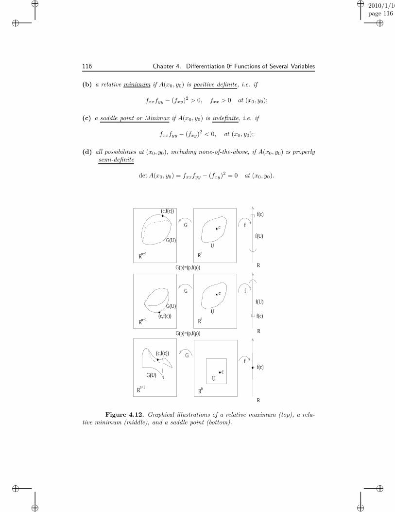
“muldowney”2010/1/10page 116
i
i
i
i
i
i
i
i
116 Chapter 4. Differentiation 0f Functions of Several Variables
(b) a relative minimum if A(x0, y0) is positive definite, i.e. if
fxxfyy − (fxy)2 > 0, fxx > 0 at (x0, y0);
(c) a saddle point or Minimax if A(x0, y0) is indefinite, i.e. if
fxxfyy − (fxy)2 < 0, at (x0, y0);
(d) all possibilities at (x0, y0), including none-of-the-above, if A(x0, y0) is properlysemi-definite
detA(x0, y0) = fxxfyy − (fxy)2 = 0 at (x0, y0).
��
��������
R R
R
fG c
(c,f(c))
G(U)U
n+1 n
f(c)
f(U)
G(p)=(p,f(p))
��
��������
R R
R
fG c
G(U)U
n+1 n
f(U)
G(p)=(p,f(p))
(c,f(c)) f(c)
��
��
��c
f(c)
R
RR
Gf
UG(U)
(c,f(c))
n+1 n
Figure 4.12. Graphical illustrations of a relative maximum (top), a rela-tive minimum (middle), and a saddle point (bottom).
“muldowney”2010/1/10page 117
i
i
i
i
i
i
i
i
4.3. Partial Derivatives of Higher Order 117
Example 4.41 For the function f(x, y) = x2 + xy + y2, from the equations fx =2x+ y = 0 and fy = x+ 2y = 0, we find that (x, y) = (0, 0) is the only stationarypoint. Now [
fxx(x, y) fxy(x, y)fyx(x, y) fyy(x, y)
]=
[2 11 2
],
satisfies fxx(0, 0) = 2 > 0 and 2 · 2 − 12 = 3 > 0, so that the matrix is positivedefinite and f has a relative minimum at (0, 0). In fact, it is a global minimumsince the matrix above is positive definite for all (x, y), so that the remainder inTaylor’s Theorem R2(x, y) > 0 for any (x, y) 6= (0, 0).
Example 4.42 For the function f(x, y) = x2 + 4xy + y2, from the equations fx =2x+4y = 0 and fy = 4x+2y = 0, we find that (x, y) = (0, 0) is the only stationarypoint, but in this case
[fxx(x, y) fxy(x, y)fyx(x, y) fyy(x, y)
]=
[2 44 2
], satisfies 2 · 2− 42 = −12 < 0
so the matrix is indefinite. Hence, f has a saddle point at (0, 0). Alternately onecan see this from the observation that f(x, y) > 0 on the coordinate axes except atthe origin, but is negative on the line y = −x when x > 0.
Example 4.43 For the function f(x, y) = 3x2 − y2 + x3, from the equations
fx = 6x+ 3x2 = 3x(2 + x) = 0, and fy = −2y = 0,
we see that the stationary points are (0, 0) and (−2, 0). We observe
for (0, 0)
[6 00 −2
]is indefinite =⇒ saddle point
for (−2, 0)
[−6 00 −2
]is negative definite =⇒ relative maximum.
Example 4.44 For the function f(x, y) = x4 + y4, from the equations
fx = 4x3 = 0, and fy = 4y3 = 0,
we see that the stationary point is (0, 0). We observe
[fxx(x, y) fxy(x, y)fyx(x, y) fyy(x, y)
]=
[12x2 0
0 12y2
], has zero determinant at (0, 0).
Thus, we have no information from the theorem. However, 12x2 ≥ 0, 12y2 ≥ 0 and144x2y2 ≥ 0 so that the matrix is positive semidefinite for all (x, y) and positivedefinite if x 6= 0 and y 6= 0. Thus, the remainder in Taylor’s theorem R2(x, y) ≥ 0for all (x, y) and f has a minimum at (0, 0). Of course, one can easily observe thatf(x, y) > 0 when (x, y) 6= (0, 0) without resorting to second derivatives.
“muldowney”2010/1/10page 118
i
i
i
i
i
i
i
i
118 Chapter 4. Differentiation 0f Functions of Several Variables
Example 4.45 For the function f(x, y) = x4 − y4, from the equations
fx = 4x3 = 0, and fy = −4y3 = 0,
we see that the stationary point is (0, 0). We observe[fxx(x, y) fxy(x, y)fyx(x, y) fyy(x, y)
]=
[12x2 0
0 −12y2
], has zero determinant at (0, 0).
However, the matrix is positive semidefinite on the line y = 0 and negative semidefiniteon x = 0 so that (0, 0) is a saddle point. In this case, it is also obvious withoutconsidering second order partials that
f(x, 0) > f(0, 0) if x 6= 0 and f(0, y) < f(0, 0) if y 6= 0.
The last two examples illustrates the fact that anything can happen in the casethat fxxfyy−(fxy)
2 = 0 at a stationary point. Our next example looks at a functionon R3. However, we need some more applicable criteria for the definitiveness of amatrix.
The following criteria may be found, say, in the book by Gantmacher, Matrix
Theory.
Theorem 4.46. Let A be a symmetric n× n matrix. Then
(a) A is positive semidefinite if and only if the determinants of all the k × k sub-matrices of A symmetric about the main diagonal are non-negative (≥ 0).
(b) A is negative semidefinite if and only if the determinants of all the k × k sub-
matrices of A symmetric about the main diagonal have sign (−1)k or are zero.
(c) A is positive definite if and only if the determinants
det
a1,1 . . . a1,k
... . . ....
ak,1 . . . ak,k
> 0, k = 1, 2, . . . , n.
(d) A is negative definite if and only if the determinants
(−1)k det
a1,1 . . . a1,k
... . . ....
ak,1 . . . ak,k
> 0, k = 1, 2, . . . , n.
(e) A is indefinite if and only if it satisfies none of (a), (b), (c), or (d).
The determinants in parts (c) and (d) are sometimes called the principal mi-nors.
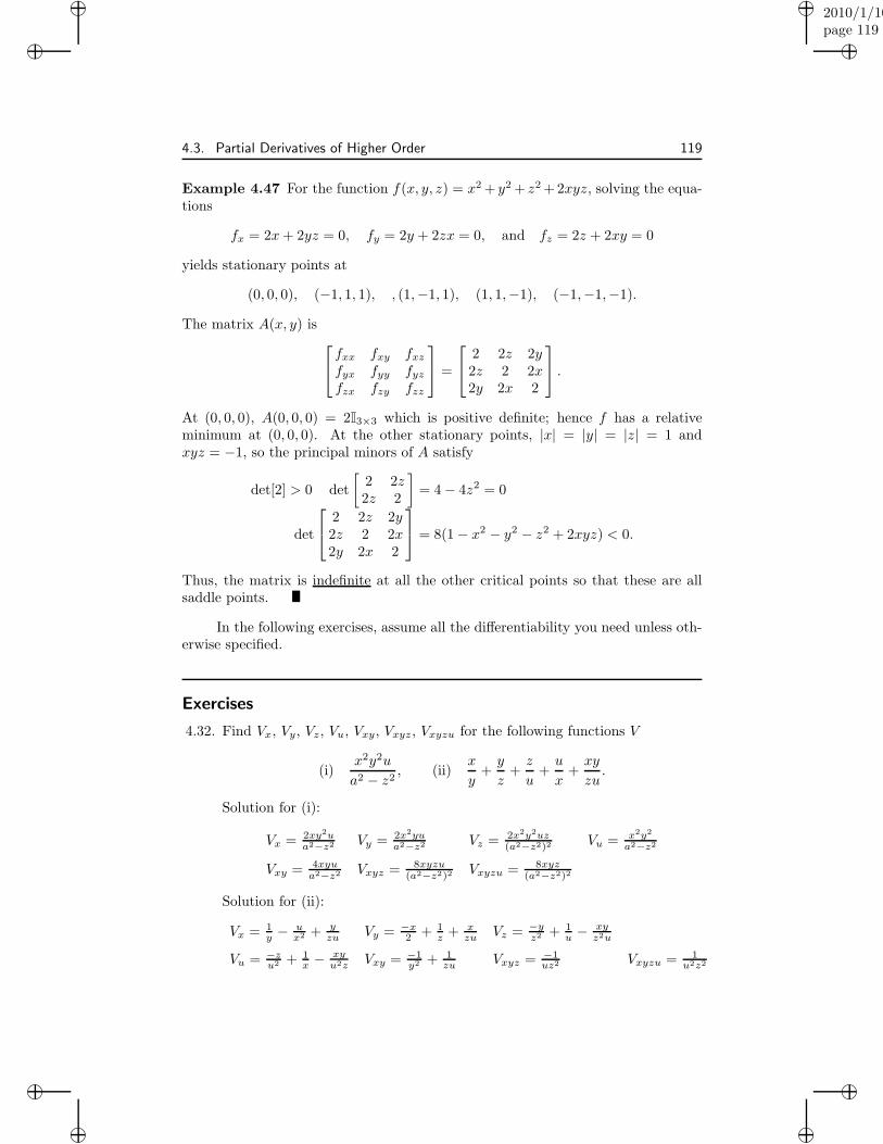
“muldowney”2010/1/10page 119
i
i
i
i
i
i
i
i
4.3. Partial Derivatives of Higher Order 119
Example 4.47 For the function f(x, y, z) = x2 + y2 + z2 +2xyz, solving the equa-tions
fx = 2x+ 2yz = 0, fy = 2y + 2zx = 0, and fz = 2z + 2xy = 0
yields stationary points at
(0, 0, 0), (−1, 1, 1), , (1,−1, 1), (1, 1,−1), (−1,−1,−1).
The matrix A(x, y) isfxx fxy fxzfyx fyy fyzfzx fzy fzz
=
2 2z 2y2z 2 2x2y 2x 2
.
At (0, 0, 0), A(0, 0, 0) = 2I3×3 which is positive definite; hence f has a relativeminimum at (0, 0, 0). At the other stationary points, |x| = |y| = |z| = 1 andxyz = −1, so the principal minors of A satisfy
det[2] > 0 det
[2 2z2z 2
]= 4− 4z2 = 0
det
2 2z 2y2z 2 2x2y 2x 2
= 8(1− x2 − y2 − z2 + 2xyz) < 0.
Thus, the matrix is indefinite at all the other critical points so that these are allsaddle points.
In the following exercises, assume all the differentiability you need unless oth-erwise specified.
Exercises
4.32. Find Vx, Vy, Vz, Vu, Vxy, Vxyz, Vxyzu for the following functions V
(i)x2y2u
a2 − z2, (ii)
x
y+y
z+z
u+u
x+xy
zu.
Solution for (i):
Vx = 2xy2ua2−z2 Vy = 2x2yu
a2−z2 Vz = 2x2y2uz(a2−z2)2 Vu = x2y2
a2−z2
Vxy = 4xyua2−z2 Vxyz = 8xyzu
(a2−z2)2 Vxyzu = 8xyz(a2−z2)2
Solution for (ii):
Vx = 1y − u
x2 + yzu Vy = −x
2 + 1z + x
zu Vz = −yz2 + 1
u −xyz2u
Vu = −zu2 + 1
x −xyu2z Vxy = −1
y2 + 1zu Vxyz = −1
uz2 Vxyzu = 1u2z2
“muldowney”2010/1/10page 120
i
i
i
i
i
i
i
i
120 Chapter 4. Differentiation 0f Functions of Several Variables
4.33. If V = x2 − y2, x = 3u− 4v + 2, y = 2u + 3v − 1, show that Vu = 6x − 4y,Vv = −8x− 6y.
4.34. If V = x3 + 8y3 − 18xy, find the points (x, y) at which Vx = Vy = 0 andinvestigate the nature of V at these points [Solution: (0, 0) is a saddle point,(3, 3/2) is a minimum.]
4.35. If P = x2y − y3 − y2z, Q = xy2 − x3 − x2z, R = xy2 + x2y, show thatP (Qz −Ry) +Q(Rx − Pz) +R(Py −Qx) = 0.
4.36. If u = x+ y + z, v = x2 + y2 + z2, w = x3 + y3 + z3 − 3xyz, show
∂(u, v, w)
∂(x, y, z)= 0.
4.37. If V, P,Q,R are C1 functions of (x, y, z) satisfying the relations
Vx = µP, Vy = µQ, , Vz = µR, for some µ 6= 0,
show that
P (Qz −Ry) +Q(Rx − Pz) +R(Py −Qx) = 0.
4.38. Let P,Q : R2 7→ R, with P,Q, ∂P∂y ,∂Q∂x continuous.
(i) Prove that there is a real valued function f on R2 such that
f ′(x, y) = [P (x, y) Q(x, y) ]
if and only if ∂P∂y = ∂Q
∂x . [HINT: “Only if” easy. ”If” – consider
f(x, y) =
∫ x
x0
P (t, y0) dt+
∫ y
y0
Q(x, t) dt.
See Exercise 32 (ii).]
(ii) State what you would consider to be a generalization of part (i) forfunctions of three variables.
(iii) Verify that each of the following is the Jacobian matrix f ′(x, y) of somefunction f(x, y) and find f(x, y):
(a) [ 2xy x2 + 3y2 ] , (b) [ 2ye2x + 2x cos(y) e2x − x2 sin(y) ] .
4.39. If F (x, y) = x/(x2 + y2) and G(x, y) = y/(x2 + y2), show that
(i) Fy = Gx, Fx = −Gy(ii) ∇2F = ∇2G = 0 where ∇2 = ∂2
∂x2 + ∂2
∂y2 .
4.40. Show the following:
(i) If V = V (x, y), x = x(u, v), and y = y(u, v), then
“muldowney”2010/1/10page 121
i
i
i
i
i
i
i
i
4.3. Partial Derivatives of Higher Order 121
(a) [Vu Vv ] = [Vx Vy ]
[xu xvyu yv
]
(b)
[Vuu VuvVvu Vvv
]=
[xu yuxv yv
] [Vxx VxyVyx Vyy
] [xu xvyu yv
]
+ Vx
[xuu xuvxvu xvv
]+ Vy
[yuu yuvyvu yvv
].
(ii) If U = U(x, y), V = V (x, y), x = x(u, v), y = y(u, v), show that
∂(U, V )
∂(u, v)=∂(U, V )
∂(x, y)
∂(x, y)
∂(u, v).
[Hint: Use (i)(a)]
(iii) If x = r cos(θ), y = r sin(θ), show
∂(U, V )
∂(x, y)=
1
r
∂(U, V )
∂(r, θ).
4.41. If V = 3x2 + 2y2 + φ(x2 − y2), prove that
yVx + xVy = 10xy.
4.42. If V = x2 + y2 + φ(xy) + ψ(y/x), prove that
x2Vxx − y2Vyy + xVx − yVy = 4(x2 − y2).
4.43. If V = V (x, y), x = ρ cos(φ), y = ρ sin(φ), show that
∇2V := Vxx + Vyy = Vρρ +1
ρVρ +
1
ρ2Vφφ.
[Hint: ρ =√x2 + y2, φ = arctan(y/x).]
4.44. If V = V (r, θ), ρ = c2/r, φ = 2π − θ, show that
ρ2Vρρ + ρVρ + Vφφ = r2Vrr + rVr + Vθθ.
4.45. If V = V (x, y), x = x(u, v), y = y(u, v), and xu = yv, xv = −yu, show
Vuu + VvvVxx + Vyy
= x2u + x2
v = y2u + y2
v.
4.46. (Euler’s Theorem continued, see Exercise 31) If V is a homogeneous functionof (x, y, z) of the mth degree, show that
x2Vxx + y2Vyy + z2Vzz + 2xyVxy + 2yzVyz + 2zxVzx = m(m− 1)V.
“muldowney”2010/1/10page 122
i
i
i
i
i
i
i
i
122 Chapter 4. Differentiation 0f Functions of Several Variables
4.47. If zy = F (zz), F′ 6= 0, then zxxzyy = z2
xy.
4.48. If z = xF (x + y) +G(x + y), show that
zxx − 2zxy + zyy = 0.
4.49. Do the following:
(a) If z = F (y+m1x)+G(y+m2x) andm1,m2 are the roots of the quadraticequation am2 +2hm+ b, then verify that azxx+2hzxy+ bzyy = 0. Showthis equation is satisfied by z = xF (y + m1x) + G(y + m2x) if m is adouble root of the quadratic equation.
(b) The equation of lateral vibration of a taut string is
ztt − c2zxx = 0.
Deduce from (a) that z = F (x+ ct) +G(x − ct) is a solution.
(c) A vibrating string for which initial displacement and velocity are specifiedis governed by relations of the form
ztt − c2zxx = 0, z(x, 0) = f(x), zt(x, 0) = g(x).
Show that
z(x, t) =1
2{f(x+ ct) + f(x− ct)} +
1
2c
∫ x+ct
x−ctg
is a solution to this problem.
4.50. Do the following:
(a) If z = xφ(y/x) + ψ(y/x), then
x2zxx + 2xyzxy + y2zyy = 0.
(b) If z = x3φ(y/x) + ψ(y/x)/x3, then
x2zxx + 2xyzxy + y2zyy + xzx + yzy = 9z.
[Hint: If you are observant you don’t have to do all that differentiation.]
4.51. Discuss the nature of the stationary points of the functions
(a) 34x2 − 24xy + 41y2. [Solution: (0, 0) is a minimum.]
(b) 3x2 + 4xy − 4y2. [Solution: (0, 0) is a saddle.]
(c) x2y − 4x2 − y2. [Solution: (0, 0) is a max; (±2√
2, 4) are saddles.]
(d) x2y+2x2−2xy+3y2−4x+7y. [Solution: (1,−1) is a min; (1±√
6,−2)are saddles.]
(e) x2yz − 2xyz + x2z + x2 + y2 + z2 + yz − 2xz − 2x + 2y + z. [Solution:(1,−1, 0) is a min; (1±
√2,−2, 1) and (1 ±
√2, 0,−1) are saddles.]
“muldowney”2010/1/10page 123
i
i
i
i
i
i
i
i
4.3. Partial Derivatives of Higher Order 123
4.52. Show that the function
f(x, y) = (y − x2)(y − 2x2)
does not have a relative extrema at (0, 0) even though it has a relativeminimum at this point when the domain is restricted to any line x = t,y = αt. [In the (x, y)-plane sketch the curves f(x, y) = 0, then determinethe regions f(x, y) < 0, f(x, y) > 0; check that on each line through (0, 0),f(x, y) > 0 = f(0, 0) if (x, y) is close enough to (0,0).]
4.53. Show that the box of maximum volume which can be inscribed in the ellipsoid
x2
a2+y2
b2+z2
c2= 1
has sides of length 2a/√
3, 2b/√
3, 2c/√
3.
4.54. Suppose we are given n points (xj , yj) ∈ R2 and desire to find a functionF (x) = Ax+B for which the quantity
n∑
j=1
(F (xj)− yj
)2
is minimized. Show that this problem leads to the equations
A∑n
j=1 x2j +B
∑nj=1 xj =
∑nj=1 xjyj
A∑n
j=1 xj + nB =∑nj=1 yj
which are easily solved for A and B. The line y = Ax + B is the line whichbest fits the given set of points in the sense of least squares.
4.55. Let {φk} be a sequence of real-valued continuous functions on [a, b] such that
∫ b
a
φkφm =
{1, if k = m;0, if k 6= m,
Let f be a real-valued continuous function on [a, b]. Prove that the choice ofconstants γ1, . . . , γℓ which minimizes the quantity
∫ b
a
(f −
ℓ∑
k=1
γkφk
)2
,
for a given ℓ is
γk =
∫ b
a
fφk, k = 1, . . . , ℓ.
This problem arises in the theory of Fourier Series.
4.56. The capacity of a condenser formed by two concentric spherical conductorsof radii a and b, 0 < a < b, is
C(a, b) =ab
b− a .
“muldowney”2010/1/10page 124
i
i
i
i
i
i
i
i
124 Chapter 4. Differentiation 0f Functions of Several Variables
Suppose that in measuring the radii of a and b of the spheres the measure-ments are subject to errors of amount δa and δb respectively. Given thatproducts of the errors are negligible relative to the other quantities involvedderive the following approximation on the error in C:
δC
C≈ δa
a
b
b− a −δb
b
a
b− a .
4.57. The breaking weight W of a cantilever beam is given by the formula Wℓ =kbd2 where b is breadth, ℓ is length, d is depth, and k is a constant dependingon the material of the beam. If the breadth is increased by 2% and the depthby 5%, show that the length should be increased by about 12% if the breakingweight is to remain unchanged.
4.58. In a triangle ABC, the area is calculated from the elements a, B, C, themeasurements being subject to errors δa, δB, δC. Show that the error δS inthe area is approximately given by
δS
S≈ 2
δa
a+
cδB
a sin(B)+
bδC
a sinC.
4.59. Let f : R2 7→ R, be f of class C2 on a convex subset D of R2. Suppose thatat each point p ∈ D, the matrix
[fxx fxyfyx fyy
]
is positive semidefinite. Prove that if p,q ∈ D, then
f
(p + q
2
)≤ 1
2
(f(p) + f(q)
).
What does this result mean geometrically?
4.4 Local Properties of C1 Functions
Recall that if f : Rn 7→ Rn, that is f(p) = (f1(p), . . . , fn(p)), p = (x1, . . . , xn), isdifferentiable at p0, then the Jacobian of f at p0 is
det f ′(p0) =
∣∣∣∣∣∣∣
∂f1∂x1
. . . ∂f1∂xn
......
...∂fn
∂x1. . . ∂fn
∂xn
∣∣∣∣∣∣∣p0
=∂(f1, . . . , fn)
∂(x1, . . . , xn)= Jf (p0).
Definition 4.48. A function f is locally one-to-one on a subset D of its domainif there is a neighborhood U of p ∈ D on which f is one-to-one.
Lemma 4.49. If f : Rn 7→ Rn is of class C1 at p0 and Jf (p0) 6= 0, then there isa neighborhood U of p0 on which f is one-to-one.
“muldowney”2010/1/10page 125
i
i
i
i
i
i
i
i
4.4. Local Properties of C1 Functions 125
Proof. Since the partials of f are continuous at p0 and Jf (p0) 6= 0, there is aconvex neighborhood U of p0 such that if pi ∈ U , i = 1, . . . , n, then
∣∣∣∣∣∣∣
∂f1∂x1
(p1) . . . ∂f1∂xn
(p1)
......
...∂fn
∂x1(pn) . . . ∂fn
∂xn(pn)
∣∣∣∣∣∣∣6= 0. (4.16)
If a,b ∈ U , then, applying the Mean-Value Theorem to each component of f , wefind
f1(b)− f1(a) =∑ni=1(bi − ai)∂f1∂xi
(p1)...
......
fn(b)− fn(a) =∑ni=1(bi − ai)∂fn
∂xi(pn)
(4.17)
where pi., i = 1, . . . , n, are some points on the line segment between a and b. But(4.16) and (4.17) imply
(fi(b)− fi(a) = 0, i = 1, . . . , n)⇐⇒ b− a = 0
since the system of equations has full rank. Thus, f(a) = f(b) if and only if a = band f is one-to-one on U .
The following is an immediate consequence of this lemma:
Theorem 4.50. Let f : Rn 7→ Rm, m ≥ n. Suppose D is an open subset of Rn
and
(i) f ∈ C1(D)
(ii) rank f ′(p) = n, for all p ∈ D,
then f is locally one-to-one on D.
Proof. Suppose f = (f1, . . . , fm), m ≥ n. We wish to show that f is one-to-oneon a neighborhood U of each point p0 ∈ D. Since rankf ′(p0) = n, we may assumewithout loss of generality that
∂(f1, . . . , fn)
∂(x1, . . . , xn)(p0) 6= 0.
(This can be achieved by relabelling the f ’s.) Thus, if f : Rn 7→ Rn is defined byf = (f1, . . . , fn), then f ∈ C1(D) and Jf (p0) 6= 0, so by the Lemma, f is one-to-
one on a neighborhood of p0. But since f(p) = f(q) implies f(p) = f(q), f beingone-to-one implies f is one-to-one.
Example 4.51 This example shows that in the preceding theorem, f need not beglobally one-to-one. Take f(x, y) = (ex cos(y), ex sin(y)). Then
Jf (x, y) =
∣∣∣∣ex cos(y) −ex sin(y)
ex sin(y) ex cos(y)
∣∣∣∣ = e2x 6= 0, for all (x, y) ∈ R2.
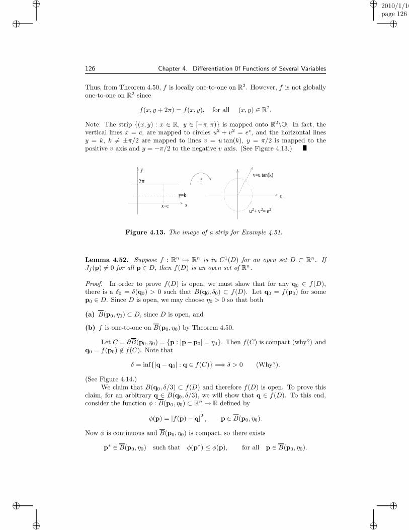
“muldowney”2010/1/10page 126
i
i
i
i
i
i
i
i
126 Chapter 4. Differentiation 0f Functions of Several Variables
Thus, from Theorem 4.50, f is locally one-to-one on R2. However, f is not globallyone-to-one on R2 since
f(x, y + 2π) = f(x, y), for all (x, y) ∈ R2.
Note: The strip {(x, y) : x ∈ R, y ∈ [−π, π)} is mapped onto R2\O. In fact, thevertical lines x = c, are mapped to circles u2 + v2 = ec, and the horizontal linesy = k, k 6= ±π/2 are mapped to lines v = u tan(k), y = π/2 is mapped to thepositive v axis and y = −π/2 to the negative v axis. (See Figure 4.13.)
u + v = e
u
v=u tan(k)
x
y
y=k
x=c
2π
2 2 2
f
Figure 4.13. The image of a strip for Example 4.51.
Lemma 4.52. Suppose f : Rn 7→ Rn is in C1(D) for an open set D ⊂ Rn. IfJf (p) 6= 0 for all p ∈ D, then f(D) is an open set of Rn.
Proof. In order to prove f(D) is open, we must show that for any q0 ∈ f(D),there is a δ0 = δ(q0) > 0 such that B(q0, δ0) ⊂ f(D). Let q0 = f(p0) for somep0 ∈ D. Since D is open, we may choose η0 > 0 so that both
(a) B(p0, η0) ⊂ D, since D is open, and
(b) f is one-to-one on B(p0, η0) by Theorem 4.50.
Let C = ∂B(p0, η0) = {p : |p−p0| = η0}. Then f(C) is compact (why?) andq0 = f(p0) 6∈ f(C). Note that
δ = inf{|q− q0| : q ∈ f(C)} =⇒ δ > 0 (Why?).
(See Figure 4.14.)We claim that B(q0, δ/3) ⊂ f(D) and therefore f(D) is open. To prove this
claim, for an arbitrary q ∈ B(q0, δ/3), we will show that q ∈ f(D). To this end,consider the function φ : B(p0, η0) ⊂ Rn 7→ R defined by
φ(p) = |f(p)− q|2 , p ∈ B(p0, η0).
Now φ is continuous and B(p0, η0) is compact, so there exists
p∗ ∈ B(p0, η0) such that φ(p∗) ≤ φ(p), for all p ∈ B(p0, η0).
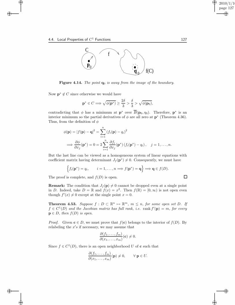
“muldowney”2010/1/10page 127
i
i
i
i
i
i
i
i
4.4. Local Properties of C1 Functions 127
��
����
f(C)
fC
pq 0
0
Figure 4.14. The point q0 is away from the image of the boundary.
Now p∗ 6∈ C since otherwise we would have
p∗ ∈ C =⇒√φ(p∗) ≥ 2δ
3>δ
3>√φ(p0),
contradicting that φ has a minimum at p∗ over B(p0, η0). Therefore, p∗ is aninterior minimum so the partial derivatives of φ are all zero at p∗ (Theorem 4.36).Thus, from the definition of φ
φ(p) = |f(p)− q|2 =n∑
i=1
(fi(p)− qi)2
=⇒ ∂φ
∂xj(p∗) = 0 = 2
n∑
i=1
∂fi∂xj
(p∗) (fi(p∗)− qi) , j = 1, . . . , n.
But the last line can be viewed as a homogeneous system of linear equations withcoefficient matrix having determinant Jf (p
∗) 6= 0. Consequently, we must have{fi(p
∗) = qi, i = 1, . . . , n =⇒ f(p∗) = q}
=⇒ q ∈ f(D).
The proof is complete, and f(D) is open.
Remark: The condition that Jf (p) 6= 0 cannot be dropped even at a single pointin D. Indeed, take D = R and f(x) = x2. Then f(R) = [0,∞) is not open eventhough f ′(x) 6= 0 except at the single point x = 0.
Theorem 4.53. Suppose f : D ⊂ Rn 7→ Rm, m ≤ n, for some open set D. Iff ∈ C1(D) and the Jacobian matrix has full rank, i.e. rank f ′(p) = m, for everyp ∈ D, then f(D) is open.
Proof. Given c ∈ D, we must prove that f(c) belongs to the interior of f(D). Byrelabeling the x′s if necessary, we may assume that
∂(f1, . . . , fm)
∂(x1, . . . , xm)(c) 6= 0.
Since f ∈ C1(D), there is an open neighborhood U of c such that
∂(f1, . . . , fm)
∂(x1, . . . , xm)(p) 6= 0, ∀ p ∈ U.
“muldowney”2010/1/10page 128
i
i
i
i
i
i
i
i
128 Chapter 4. Differentiation 0f Functions of Several Variables
Define f : Rm 7→ Rm on the open set
U := {(x1, . . . , xm) : (x1, . . . , xm, cm+1, . . . , cn) ∈ U}
by
f(x1, . . . , xm) = f(x1, . . . , xm, cm+1, . . . , cm).
Then f ∈ C1(U) and Jf (x1, . . . , xm) 6= 0, for all (x1, . . . , xm) ∈ U . From Lemma
4.52, f(U) is an open set in Rm. Hence
f(c) = f(c1, . . . , cm) ∈ f(U) ⊂ f(U) ⊂ f(D)
=⇒ f(c) ∈ f(D)◦, ∀ c ∈ D,
and so f(D) is open.
Question: In the proof it was stated that U was open, why is that true?
Lemma 4.54. If f is continuous and one-to-one on a compact set S, then the
inverse function f−1 is continuous on f(S).
Proof. Let q0 ∈ f(S). We wish to show f−1 is continuous at q0. If f−1 were notcontinuous, then for some ǫ0 > 0, there is a sequence of points {qk} ⊂ f(S) forwhich
limk→∞
qk = q0 and∣∣f−1(qk)− f−1(q0)
∣∣ ≥ ǫ0. (4.18)
Now the image of the sequence, {f−1(qk)} is a sequence in the compact set S, hencethere is a subsequence {f−1(qkj
)} such that
limj→∞
f−1(qkj) = p1 ∈ S. (4.19)
By (4.18), p1 6= f−1(q0). But f is continuous at p1 and f is one-to-one so, from(4.19),
limj→∞
qkj= lim
j→∞f(f−1(qkj
))
= f(p1) 6= f(f−1(q0)
)= q0,
a contradiction. Thus, f−1 must be continuous at q0.
In general, the requirement that S be compact cannot be dropped. It cannoteven be replaced by the requirement that f(S) be compact as the next exampleshows:
Example 4.55 Let f : [0, 2π) 7→ {x2+y2 = 1}, be defined by f(θ) = (cos(θ), sin(θ)).Then f ∈ C([0, 2π)), f is one-to-one and f([0, 2π)) is compact in R2. However, f−1
is discontinuous at (1, 0) (nearby points on the circle on either side of this point areat opposite ends of the interval under f−1).

“muldowney”2010/1/10page 129
i
i
i
i
i
i
i
i
4.4. Local Properties of C1 Functions 129
Lemma 4.56. Let f : Rn 7→ Rn. If f ∈ C1 in a neighborhood of p0 and Jf (p0) 6= 0,then there is a neighborhood U of p0 and a constant m > 0 such that
p ∈ U =⇒ |f(p)− f(p0)| ≥ m |p− p0| .
Proof. Since Jf (p0) 6= 0, the differential Df(p0) : Rn 7→ Rn is one-to-one. There-fore, there exists m > 0 such that
|Df(p0)(u)| ≥ 2m|u|, for all u ∈ Rn (Theorem 4.7),
=⇒ |Df(p0)(p− p0)| ≥ 2m|p− p0|, for all p.(4.20)
But from the definition of Df(p0), there is a neighborhood U of p0 such that
p ∈ U =⇒ |f(p)− f(p0)−Df(p0)(p− p0)| ≤ m|p− p0|. (4.21)
But then
m|p− p0| ≥ |f(p)− f(p0)−Df(p0)(p− p0)|≥ |Df(p0)(p− p0)| − |f(p)− f(p0)|≥ 2m|p− p0| − |f(p)− f(p0)| by (4.21)
=⇒ m|p− p0| ≤ |f(p)− f(p0)|.
We are now in a position to say something about the differentiability of theinverse function.
Theorem 4.57. Let f : Rn 7→ Rn, and suppose
(i) D is an open set of Rn, f ∈ C1(D), and Jf (p) 6= 0 at every p ∈ D, and
(ii) f is one-to-one-on D.
Then f−1 ∈ C1(f(D)) and Df−1 = (Df)−1 (the inverse matrix).
Proof. Let g : Rn 7→ Rn be defined by
g(p) :=1
|p− p0|(f(p)− f(p0)−Df(p0)(p − p0)
)(4.22)
=⇒ limp→p0
g(p) = O, (by definition of Df(p0).). (4.23)
Since Jf (p0) 6= 0, the inverse matrix(Df(p0)
)−1exists and from (4.22),
|p− p0|(Df(p0)
)−1g(p) =
(Df(p0)
)−1(f(p)− f(p0)−Df(p0)(p− p0)
)
=(Df(p0)
)−1(f(p)− f(p0)
)− (p− p0).
(4.24)
“muldowney”2010/1/10page 130
i
i
i
i
i
i
i
i
130 Chapter 4. Differentiation 0f Functions of Several Variables
By Theorem 4.53, f(D) is open and, in particular, it is a neighborhood off(p0). Hence, with q0 = f(p0) and q = f(p), we may deduce from (4.24) andLemma 4.56 that
1
m|q−q0||
(Df(p0)
)−1(g(p))| ≥
∣∣∣f−1(q) − f−1(q0)−(Df(p0)
)−1(q− q0)
∣∣∣ (4.25)
if p is in some neighborhood of p0. Furthermore, from Lemma 4.54, f and f−1 arecontinuous at p0 and q0 respectively, so that
q→ q0 =⇒ f−1(q)→ f−1(q0) =⇒ p→ p0.
Therefore, from (4.25) and (4.23) we deduce
limq→q0
∣∣∣f−1(q)− f−1(q0)−(Df(p0)
)−1(q− q0)
∣∣∣|q− q0|
= 0,
sincelim
q→q0
(Df(p0)
)−1(g(p)) = lim
p→p0
(Df(p0)
)−1(g(p)) = 0.
Thus, since(Df(p0)
)−1is linear, Df−1 exists and equals
(Df(p0)
)−1.
From the fact thatDf−1(f(p0)) =(Df(p0)
)−1, it follows that f−1 ∈ C1(f(D))
since the partial derivatives of f−1 are rational functions of the partial derivativesof f in which the denominator Jf (p) is not zero.
Example 4.58 We have seen that f(x, y) = (ex cos(y), ex sin(y)) is one-to-one onthe strip 0 ≤ y < 2π. Recall
det f ′(x, y) = det
[ex cos(y) −ex sin(y)
ex sin(y) ex cos(y)
]= e2x 6= 0,
=⇒ [f ′(x, y)]−1
= e−2x
[ex cos(y) ex sin(y)
−ex sin(y) ex cos(y)
].
To find f−1, solve (u, v) = (ex cos(y), ex sin(y)) for x and y:
u2 + v2 = e2x, tan(y) =v
u
=⇒ x =1
2log(u2 + v2), y = arctan
( vu
)
=⇒ f−1(u, v) =
(1
2log(u2 + v2), arctan
( vu
)).
and
(f−1
)′(u, v) =
[ uu2+v2
vu2+v2
−vu2+v2
uu2+v2
]=
1
u2 + v2
[u v−v u
]
= e−2x
[ex cos(y) ex sin(y)
−ex sin(y) ex cos(y)
].
“muldowney”2010/1/10page 131
i
i
i
i
i
i
i
i
4.5. Implicit Function Theorem 131
Thus, we see that Df−1(u, v) =(Df(x, y)
)−1
.
Exercises
4.60. In Exercise 29 a sufficient condition was given for f : Rn 7→ Rn to be globallyone-to-one. Verify that this condition is not satisfied by Example 4.51. (Ifyou did not do Exercise 29, a proof is given in Lemma 4.49.)
4.61. Show that if f : R 7→ R and f ′(x) 6= 0 for each x ∈ R, then f is one-to-oneglobally on R.
4.62. Let f : R 7→ R. Show that if f is continuous and one-to-one on a connectedsubset S of R, then f−1 is continuous on f(S).
4.63. If y = y(x), that is yi = yi(x1, . . . , xn), for i = 1, . . . , n, be C1. Show that
∂(y1, . . . , yn)
∂(x1, . . . , xn)6= 0 =⇒ ∂(y1, . . . , yn)
∂(x1, . . . , xn)· ∂(x1, . . . , xn)
∂(y1, . . . , yn)= 1.
4.64. Let f(x, y) = (x2, y/x) when x > 0. Find f ′(x, y). Show that f is one-to-one
on its domain by finding f−1. Check that(f ′)−1
=(f−1
)′.
4.65. Let
f(x, y) =
(x√
x2 + y2,
y√x2 + y2
).
Show that Jf (x, y) = 0 for all (x, y) ∈ R2\O and f is not locally one-to-oneanywhere on its domain. Show that the range of f is the circle u2 + v2 = 1and thus contains no open subset.
4.5 Implicit Function Theorem
Question: If we are given a system of n equations in m+ n unknowns, when andhow can we choose n of the variables, call them y1, . . . , yn to be defined implicitlyas functions of the remaining m variables, call them x1, . . . , xm?
Writing the “independent” variables x1, . . . , xm first and the “dependent” vari-ables y1, . . . , yn second, we are asking When does the system of equations
fi(x1, . . . , xm, y1, . . . , yn) = 0, i = 1, 2, . . . , n (4.26)
uniquely define y1, . . . , yn implicitly as functions of x1, . . . , xm, i.e. when are therefunctions φi so that
yi = φi(x1, . . . , xm), i = 1, 2, . . . , n? (4.27)
Of course, the way the question was originally stated, part of the problem is tofind which are the independent variables and which are the dependent variables. Theequations will not be written for you with the independent variable so conveniently
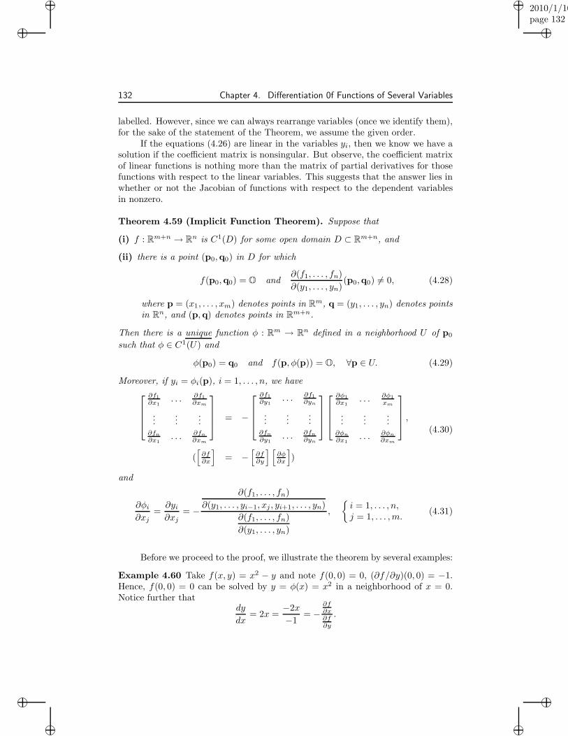
“muldowney”2010/1/10page 132
i
i
i
i
i
i
i
i
132 Chapter 4. Differentiation 0f Functions of Several Variables
labelled. However, since we can always rearrange variables (once we identify them),for the sake of the statement of the Theorem, we assume the given order.
If the equations (4.26) are linear in the variables yi, then we know we have asolution if the coefficient matrix is nonsingular. But observe, the coefficient matrixof linear functions is nothing more than the matrix of partial derivatives for thosefunctions with respect to the linear variables. This suggests that the answer lies inwhether or not the Jacobian of functions with respect to the dependent variablesin nonzero.
Theorem 4.59 (Implicit Function Theorem). Suppose that
(i) f : Rm+n → Rn is C1(D) for some open domain D ⊂ Rm+n, and
(ii) there is a point (p0,q0) in D for which
f(p0,q0) = O and∂(f1, . . . , fn)
∂(y1, . . . , yn)(p0,q0) 6= 0, (4.28)
where p = (x1, . . . , xm) denotes points in Rm, q = (y1, . . . , yn) denotes pointsin Rn, and (p,q) denotes points in Rm+n.
Then there is a unique function φ : Rm → Rn defined in a neighborhood U of p0
such that φ ∈ C1(U) and
φ(p0) = q0 and f(p, φ(p)) = O, ∀p ∈ U. (4.29)
Moreover, if yi = φi(p), i = 1, . . . , n, we have
∂f1∂x1
. . . ∂f1∂xm
......
...∂fn
∂x1. . . ∂fn
∂xm
= −
∂f1∂y1
. . . ∂f1∂yn
......
...∂fn
∂y1. . . ∂fn
∂yn
∂φ1
∂x1. . . ∂φ1
xm
......
...∂φn
∂x1. . . ∂φn
∂xm
,
([∂f∂x
]= −
[∂f∂y
] [∂φ∂x
])
(4.30)
and
∂φi∂xj
=∂yi∂xj
= −
∂(f1, . . . , fn)
∂(y1, . . . , yi−1, xj , yi+1, . . . , yn)
∂(f1, . . . , fn)
∂(y1, . . . , yn)
,
{i = 1, . . . , n,j = 1, . . . ,m.
(4.31)
Before we proceed to the proof, we illustrate the theorem by several examples:
Example 4.60 Take f(x, y) = x2 − y and note f(0, 0) = 0, (∂f/∂y)(0, 0) = −1.Hence, f(0, 0) = 0 can be solved by y = φ(x) = x2 in a neighborhood of x = 0.Notice further that
dy
dx= 2x =
−2x
−1= −
∂f∂x∂f∂y
.
“muldowney”2010/1/10page 133
i
i
i
i
i
i
i
i
4.5. Implicit Function Theorem 133
What about solving for x in terms of y? Now f(0, 0) = 0 and (∂f/∂x)(0, 0) = 0means that the condition (4.28) is not satisfied. The equation f(x, y) = 0 cannotbe solved in the form x = ψ(y) with ψ defined in a full neighborhood of y = 0.Notice there are two solutions of the form x = ±√y defined on [0,∞), but eventhese are not C1 at x = 0. There are infinitely many discontinuous solutions definedon [0,∞); for example, one is ψ(y) =
√y, y ∈ Q, ψ(y) = −√y, y 6∈ Q.
Example 4.61 Given the equations
x+ y + z = 0 (f1(x, y, z) = 0)
x2 + y2 + z2 − 2xz − 1 = 0 (f2(x, y, z) = 0)
which of the variables can be solved in terms of the others and at what points?Basically, we want to test when (4.28) holds. Therefore, we choose pairs of
variables and look at the Jacobian:
∂(f1, f2)
∂(x, y)=
∣∣∣∣1 1
2x− 2z 2y
∣∣∣∣ = 2(y − x+ z).
Therefore, we can solve for x, y as a function of z in a neighborhood of any pointexcept those lying on the plane x − z − y = 0. Substituting x = −z − y into thesecond equation gives
4z2 + 4zy + 2y2 +−1 = 0, or z2 + (z + y)2 − 1
2= 0,
which implies y = −z ±√
12 − z2. Substituting this in the first equation gives x as
a function of z.Testing another pair of variables, we find
∂(f1, f2)
∂(x, z)=
∣∣∣∣1 1
2x− 2z 2z − 2x
∣∣∣∣ = 0.
Hence, we can never solve for x, z as a function of y. One can check this directly:from the first equation y = −(x + z) which substituted into the second equationgives 2(x+ z)2 − 1 = 0, or 2y2 = 1. Thus, eliminating x also eliminates z.
Since the equations are symmetric in x and z, it should be no surprise todiscover that we can solve for z, y as a function of x in a neighborhood of any pointexcept those lying on the plane x− z − y = 0.
Example 4.62 Consider the equations
2x2 − u+ v = 0 (f1(x, y, z, u, v) = 0)
2y3 − u− v = 0 (f2(x, y, z, u, v) = 0)
z + u− v2 = 0 (f3(x, y, z, u, v) = 0)
Checking several possibilities, we find
∂(f1, f2, f3)
∂(u, v, z)=
∣∣∣∣∣∣
−1 1 0−1 −1 01 −2v 1
∣∣∣∣∣∣= 2.
“muldowney”2010/1/10page 134
i
i
i
i
i
i
i
i
134 Chapter 4. Differentiation 0f Functions of Several Variables
∂(f1, f2, f3)
∂(u, v, x)=
∣∣∣∣∣∣
−1 +1 4x−1 −1 01 −2v 0
∣∣∣∣∣∣= 4x(2v + 1)
∂(f1, f2, f3)
∂(u, v, y)=
∣∣∣∣∣∣
−1 +1 0−1 −1 6y2
1 −2v 0
∣∣∣∣∣∣= −6y2(2v − 1)
∂(f1, f2, f3)
∂(x, y, z)=
∣∣∣∣∣∣
2x 0 09 6y2 00 0 1
∣∣∣∣∣∣= 12xy2.
This shows that we can always solve for u, v, z in terms of x and y, but for the othercombinations tested, there are points at which we cannot apply the theorem. Thefirst case leads to the solution
v = y3 − x2, u = x2 + y3, z = −x2 − y3 + y6 − 2y3x2 + x4.
Example 4.63 Consider the equations
x2 − yu = 0xy + uv = 0.
(4.32)
We will view this as
f(x, y, u, v) = (x2 − yu, xy + uv) = O
and define implicitly u, v as functions of x and y in a neighborhood of (x0, y0). Thisrequires from (4.28) that we have a point (x0, y0, u0, v0) such that
x20 − y0u0 = 0, x0y0 + u0v0 = 0, and
∂(f1, f2)
∂(u, v)=
∣∣∣∣−y0 0v0 u0
∣∣∣∣ = −y0u0 6= 0.
Now, the last equation implies y0 6= 0 and u0 6= 0, and putting this in (4.32)indicates that x0 6= 0 as well. The equations are easy to solve as
u =x2
y, v =
−y2
x.
According to (4.31), we should have
∂u
∂x= −
∣∣∣∣2x 0y u
∣∣∣∣−yu =
2x
y,
∂u
∂y= −
∣∣∣∣−u 0x u
∣∣∣∣−yu = −u
y=−x2
y2
∂v
∂x= −
∣∣∣∣−y 2xv y
∣∣∣∣−yu = − y
u− 2xv
yu=−y2
x2− 2x−y2
x
x2=y2
x2
∂v
∂y= −
∣∣∣∣−y −uv x
∣∣∣∣−yu = −x
u− v
y==−2y
x.
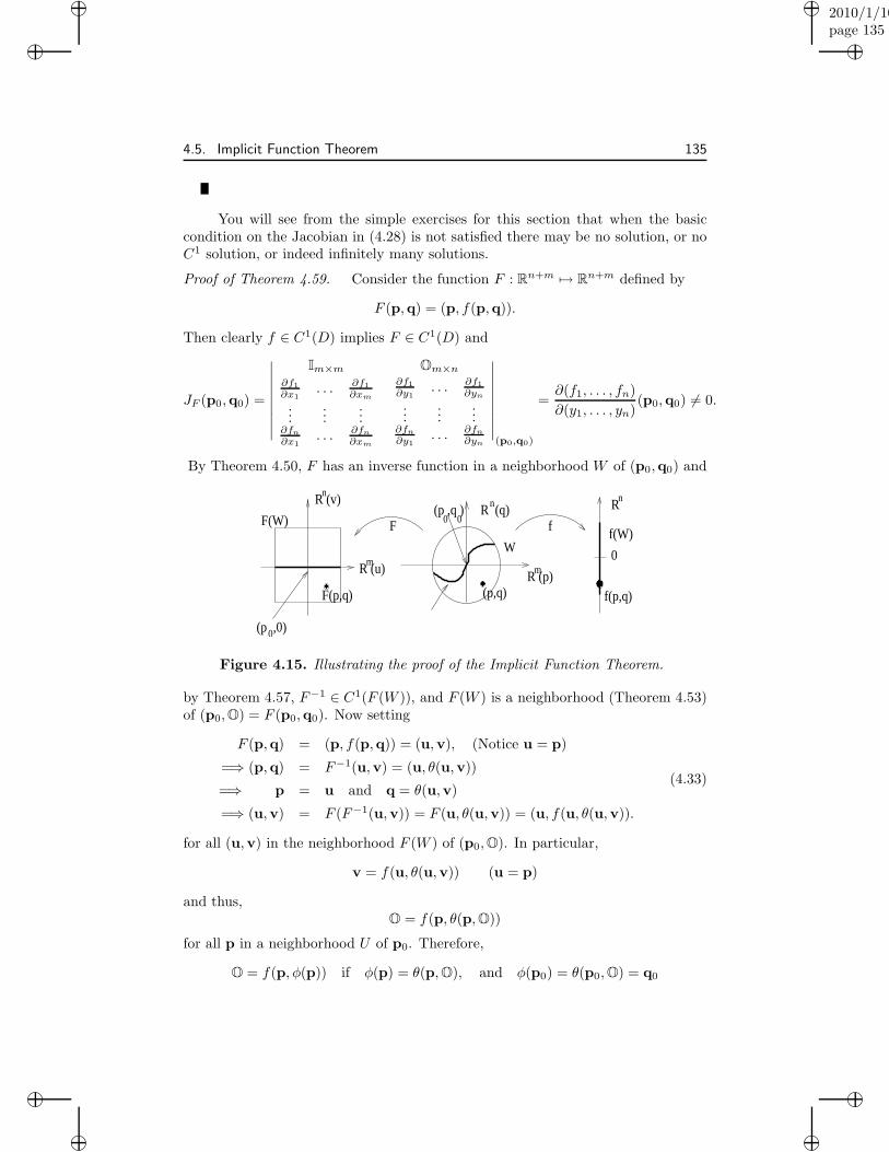
“muldowney”2010/1/10page 135
i
i
i
i
i
i
i
i
4.5. Implicit Function Theorem 135
You will see from the simple exercises for this section that when the basiccondition on the Jacobian in (4.28) is not satisfied there may be no solution, or noC1 solution, or indeed infinitely many solutions.
Proof of Theorem 4.59. Consider the function F : Rn+m 7→ Rn+m defined by
F (p,q) = (p, f(p,q)).
Then clearly f ∈ C1(D) implies F ∈ C1(D) and
JF (p0,q0) =
∣∣∣∣∣∣∣∣∣
Im×m Om×n∂f1∂x1
. . . ∂f1∂xm
......
...∂fn
∂x1. . . ∂fn
∂xm
∂f1∂y1
. . . ∂f1∂yn
......
...∂fn
∂y1. . . ∂fn
∂yn
∣∣∣∣∣∣∣∣∣(p0,q0)
=∂(f1, . . . , fn)
∂(y1, . . . , yn)(p0,q0) 6= 0.
By Theorem 4.50, F has an inverse function in a neighborhood W of (p0,q0) and
������ ����
������������������
������������������
f(p,q)
0
RR (q)
R (p)(p,q)
(p ,q )
(p ,0)
F(W)
R (u)
R (v)
f(W)W
fF
F(p,q)
mm
n n n
0 0
0
Figure 4.15. Illustrating the proof of the Implicit Function Theorem.
by Theorem 4.57, F−1 ∈ C1(F (W )), and F (W ) is a neighborhood (Theorem 4.53)of (p0,O) = F (p0,q0). Now setting
F (p,q) = (p, f(p,q)) = (u,v), (Notice u = p)
=⇒ (p,q) = F−1(u,v) = (u, θ(u,v))
=⇒ p = u and q = θ(u,v)
=⇒ (u,v) = F (F−1(u,v)) = F (u, θ(u,v)) = (u, f(u, θ(u,v)).
(4.33)
for all (u,v) in the neighborhood F (W ) of (p0,O). In particular,
v = f(u, θ(u,v)) (u = p)
and thus,O = f(p, θ(p,O))
for all p in a neighborhood U of p0. Therefore,
O = f(p, φ(p)) if φ(p) = θ(p,O), and φ(p0) = θ(p0,O) = q0
“muldowney”2010/1/10page 136
i
i
i
i
i
i
i
i
136 Chapter 4. Differentiation 0f Functions of Several Variables
so that (4.29) holds. Also φ ∈ C1(U) follows from (4.33) since F−1 ∈ C1(F (W )).To prove (4.31), we apply the Chain Rule to O = f(p, φ(p)) to obtain
O = Df(p, φ(p))
[Im×mDφ(p)
]
=⇒ 0 =∂fi∂xj
+
n∑
k=1
∂fi∂yk
∂φk∂xj
, i, j = 1, . . . ,m,
which gives (4.30). Viewing that as a linear system of equations for unknowns∂φk/∂xj, k = 1, . . . , n, Cramer’s Rule gives (4.31)
Remark: The function φ is the unique solution to f(p, φ(p)) = O with φ(p0) = q0
since if to the contrary we had two solutions
f(p, φ1(p)) = f(p, φ2(p)) = O and φ1(p) 6= φ2(p) for some p ∈ U , then
F (p, φ1(p)) = F (p, φ2(p)) = (p,O),
contradicting the fact that F is one-to-one on W . This means that the graph of φ,the set {p, φ(p)) : p ∈ U} is the whole set F−1(O) ∩W .
Corollary 4.64. Let f : R2 7→ R. If f is of class C1 in a neighborhood of (x0, y0)with
f(x0, y0) = 0 and∂f
∂y(x0, y0) 6= 0,
then the equation f(x, y) = 0 has a unique solution y = φ(x) with φ(x0) = y0, whichexists and is continuously differentiable in a neighborhood U of x0 and
φ′(x) =dy
dx= −∂f/∂x
∂f/∂y.
Corollary 4.65. Let f : R3 7→ R. If f is of class C1 in a neighborhood of (x0, y0, z0)with
f(x0, y0, z0) = 0 and∂f
∂z(x0, y0, z0) 6= 0,
then the equation f(x, y, z) = 0 has a unique solution z = φ(x, y) with φ(x0, y0) =z0, which exists and is continuously differentiable in a neighborhood U of (x0, y0)and
∂z
∂x= −∂f/∂x
∂f/∂z,
∂z
∂y== −∂f/∂y
∂f/∂z.
Corollary 4.66. Let f : R5 7→ R2. If f = (f1, f2) is of class C1 in a neighborhoodof (x0, y0, z0, u0, v0) with
{f1(x0, y0, z0, u0, v0) = 0,
f2(x0, y0, z0, u0, v0) = 0,and
∂(f1, f2)
∂(u, v)(x0, y0, z0, u0, v0) 6= 0,
“muldowney”2010/1/10page 137
i
i
i
i
i
i
i
i
4.5. Implicit Function Theorem 137
then the equations
f1(x, y, z, u, v) = 0 and f2(x, y, z, u, v) = 0
have unique solution
u = φ1(x, y, z), v = φ2(x, y, z) with u0 = φ1(x0, y0, z0), v0 = φ2(x0, y0, z0),
which exist and are continuously differentiable in a neighborhood U of (x0, y0, z0)and
∂φ1
∂x=∂u
∂x= −
∂(f1,f2)∂(x,v)
∂(f1,f2)∂(u,v)
,∂φ2
∂x=∂v
∂x= −
∂(f1,f2)∂(u,x)
∂(f1,f2)∂(u,v)
,
∂φ1
∂y=∂u
∂y= −
∂(f1,f2)∂(y,v)
∂(f1,f2)∂(u,v)
,∂φ2
∂y=∂v
∂y= −
∂(f1,f2)∂(u,y)
∂(f1,f2)∂(u,v)
,
∂φ1
∂z=∂u
∂z= −
∂(f1,f2)∂(z,v)
∂(f1,f2)∂(u,v)
,∂φ2
∂z=∂v
∂z= −
∂(f1,f2)∂(u,z)
∂(f1,f2)∂(u,v)
.
Exercises
4.66. Prove Corollary 4.64. That is, work through the proof of Theorem 4.59 inthis special case.
4.67. The equation y2−x2 = 0 has two C1 solutions, y = ±x in a neighborhood ofx = 0; this shows uniqueness may not hold. What condition of the ImplicitFunction Theorem does not hold? Check that there are four solutions of classC and infinitely many real-valued solutions.
4.68. Show that the equations
x2 − yu = 0, u = u0, v = v0, xy + uv = 0,
define u, v implicitly as functions of x and y in a neighborhood of any point(x0, y0) if y0u0 6= 0 and x0 − y0u0 = 0, x0y0 + u0v0 = 0. Check that theImplicit Function Theorem gives
∂u
∂x=
2x
y,
∂u
∂y=−uy,
∂v
∂x= − y
u− 2vx
uy,
∂v
∂y= −x
u+v
y
and verify these results by solving the equations directly.
4.69. Consider f(x, y, u, v) = (x3 + yu+ v, xv+ y3− u). At what points (x, y, u, v)can one solve f(x, y, u, v) = (0, 0) in the form (x, y) = (φ1(u, v), φ2(u, v))?Find the differential matrix
[ ∂φ1
∂u∂φ1
∂v∂φ2
∂u∂φ2
∂v
].
“muldowney”2010/1/10page 138
i
i
i
i
i
i
i
i
138 Chapter 4. Differentiation 0f Functions of Several Variables
4.70. Suppose φi(u1, . . . , un, x1, . . . , xn) = 0, i = 1, . . . , n, is satisfied by uj =uj(x1, . . . , xn), the φ’s and u’s being C1 functions. Prove that
∂(φ1, . . . , φn)
∂(u1, . . . , un)· ∂(u1, . . . , un)
∂(x1, . . . , xn)= (−1)n
∂(φ1, . . . , φn)
∂(x1, . . . , xn).
[Hint: Use the Chain Rule and think matrices.]
4.71. If u2 + v2 + 2xuv + y = 0, uv + (u + v)y + x2 = 0, prove that
∂(u, v)
∂(x, y)=
uv(u+ v)− x(u − v)[(u+ v) + y(1− x)] .
4.72. If u1 = x1 + x2 + x3 + x4, u1u2 = x2 + x3 + x4, u1u2u3 = x3 + x4, andu1u2u3u4 = x4, show that
∂(x1, x2, x3, x4)
∂(u1, u2, u3, u4)= u3
1u22u3.
4.73. Do the following
(a) If V = ψ(u, v), φ(u, v) = E(x, y), χ(u, v) = F (x, y), and ∂(φ, χ)/∂(u, v) 6=0. Prove
∂V
∂x· ∂(φ, χ)
∂(u, v)=∂E
∂x
∂(ψ, χ)
∂(u, v)+∂F
∂x· ∂(φ, ψ)
∂(u, v).
(b) If V = u2 + v2 + uv, u+ v = x2 + y2, u3 + v3 = 2xy, prove that
3∂V
∂y=
2x(x2 − y2)
(x2 + y2)2+ 8y(x2 + y2).
4.74. If V = ψ(u1, . . . , un), φk = (u1, . . . , un) = fk(x1, . . . , xm) k = 1, . . . , n, and∂(φ1, . . . , φn)/∂(u1, . . . , un) 6= 0, show that
∂V
∂xj· ∂(φ1, . . . , φn)
∂(u1, . . . , un)=
n∑
k=1
∂fk∂xj· ∂(φ1, . . . , φk−1, ψ, φk+1, . . . , φn)
∂(u1, . . . , un).
4.75. If F ∈ C1 show that the equation
F (F (x, y), y) = 0
may be solved for y as a function of x near (0, 0) provided F (0, 0) = 0,Fx(0, 0) 6= −1 and Fy(0, 0) 6= 0.
4.76. Suppose f(x, y) = 0 where f ∈ C2 and ∂f/∂y 6= 0. Prove that
d2y
dx2=
1(∂f∂y
)3
∣∣∣∣∣∣∣∣
0 ∂f∂x
∂f∂y
∂f∂x
∂2f∂x2
∂2f∂x∂y
∂f∂y
∂2f∂y∂x
∂2f∂y2
∣∣∣∣∣∣∣∣.
“muldowney”2010/1/10page 139
i
i
i
i
i
i
i
i
4.5. Implicit Function Theorem 139
4.5.1 Dimension
We have a notion of dimension for linear objects, specifically for vectors spaces,namely, the number of vectors in a basis. If L : Rk 7→ Rn is linear, L(x) = Ax, thenthe dimension of L(Rk) ⊂ Rn is the rank of A. In particular, if rankA = k, thenL(Rk) ⊂ Rn is k-dimensional, the same dimension as Rk.
Definition 4.67. A subset S of Rn is a k-dimensional segment, k > 0, if there is
an open connected set D ⊂ Rk and a function f : Rk 7→ Rn such that
(a) f ∈ C1(D) and f : D 7→ S is one-to-one and onto (i.e. f(D) = S),
(b) rank f ′(p) = k for all p ∈ D.
A 0-dimensional segment in Rn is a single point in Rn.A subset S of Rn is a k-dimensional manifold if for every q ∈ S, there exists
an open neighborhood V ⊂ Rn of q such that V ∩ S is a k-dimensional segment.
Remarks: Note that k ≤ n always. A k-dimensional segment is automatically ak-dimensional manifold. If the condition of one-to-one is dropped in (a), then f isstill locally one-to-one by Theorem 4.50, and so, f(U) is a k-dimensional segmentif U is a sufficiently small open subset of D.
Example 4.68 The set S := {(x, y) : y = 3x, 0 < x < 1} is a 1-dimensionalmanifold (segment) in R2. Indeed, let D = (0, 1) ⊂ R and define f(t) = (t, 3t),0 < t < 1. Then f ′(t) = [ 1 3 ] and rank f ′ = 1.
Example 4.69
Example 4.70 The set S := {(x, y, z) : x2+y2+z2 = 1, x > 0, y > 0, z > 0}is a 2-dimensional segment in R3. In this case, consider
f(θ, φ) :=(cos(θ) sin(φ), sin(θ) sin(φ), cos(φ)
)= (x, y, z),
{0 < θ < π
2
0 < φ < π2 .
Then f ∈ C1((0, π/2)× (0, π/2)
), f is one-to-one, and
f ′(θ, φ) =
− sin(θ) sin(φ) cos(θ) cos(φ)cos(θ) sin(φ) sin(θ) cos(φ)
0 − sin(φ)
.
Now rank f ′(θ, φ) = 2 since for example ∂(y,z)∂(θ,φ) = − cos(θ) sin2(φ) 6= 0 when 0 < θ <
π2 and 0 < φ < π
2 .
Example 4.71 The set S := {(x, y) : (x+1)2+y2 = 1}∪{(x, y) : (x−1)2+y2 = 1}is a 1-dimensional segment. This is two circles which are tangent at the origin. Weuse the mapping f : (−2π, 2π) 7→ R2 defined by
f(t) =
{(−1 + cos(t), sin(t)) if t ∈ (−2π, 0];(1 + cos(π − t), sin(π − t)), if t ∈ (0, 2π).
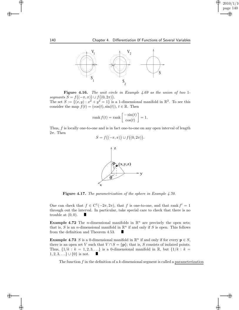
“muldowney”2010/1/10page 140
i
i
i
i
i
i
i
i
140 Chapter 4. Differentiation 0f Functions of Several Variables
������������
������������
��������������
������������
������������
������������ ����������������
�������������
�������������V
SS
S
V
1
1
2
2
Figure 4.16. The unit circle in Example 4.69 as the union of two 1-segmants S = f
((−π, π)
)∪ f((0, 2π)
).
The set S := {(x, y) : x2 + y2 = 1} is a 1-dimensional manifold in R2. To see thisconsider the map f(t) = (cos(t), sin(t)), t ∈ R. Then
rankf(t) = rank
[− sin(t)
cos(t)
]= 1.
Thus, f is locally one-to-one and is in fact one-to-one on any open interval of length2π. Then
S = f((−π, π)
)∪ f((0, 2π)
).
��������(x,y,z)
x
y
z
θ
φ
Figure 4.17. The parametrization of the sphere in Example 4.70.
One can check that f ∈ C1(−2π, 2π), that f is one-to-one, and that rank f ′ = 1through out the interval. In particular, take special care to check that there is notrouble at (0, 0).
Example 4.72 The n-dimensional manifolds in Rn are precisely the open sets;that is, S is an n-dimensional manifold in Rn if and only if S is open. This followsfrom the definition and Theorem 4.53.
Example 4.73 S is a 0-dimensional manifold in Rn if and only if for every p ∈ S,there is an open set V such that V ∩S = {p}; that is, S consists of isolated points.Thus, {1/k : k = 1, 2, 3, . . .} is a 0-dimensional manifold in R, but {1/k : k =1, 2, 3, . . .} ∪ {0} is not.
The function f in the definition of a k-dimensional segment is called a parameterization
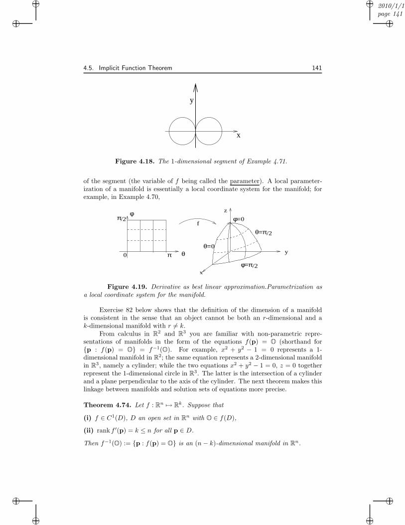
“muldowney”2010/1/10page 141
i
i
i
i
i
i
i
i
4.5. Implicit Function Theorem 141
x
y
Figure 4.18. The 1-dimensional segment of Example 4.71.
of the segment (the variable of f being called the parameter). A local parameter-ization of a manifold is essentially a local coordinate system for the manifold; forexample, in Example 4.70,
0 π
π
θ=π
φ=π
φ=
θ=θ
φ
/2
/2
/2
0
0
f
x
y
z
Figure 4.19. Derivative as best linear approximation.Parametrization asa local coordinate system for the manifold.
Exercise 82 below shows that the definition of the dimension of a manifoldis consistent in the sense that an object cannot be both an r-dimensional and ak-dimensional manifold with r 6= k.
From calculus in R2 and R3 you are familiar with non-parametric repre-sentations of manifolds in the form of the equations f(p) = O (shorthand for{p : f(p) = O} = f−1(O). For example, x2 + y2 − 1 = 0 represents a 1-dimensional manifold in R2; the same equation represents a 2-dimensional manifoldin R3, namely a cylinder; while the two equations x2 + y2 − 1 = 0, z = 0 togetherrepresent the 1-dimensional circle in R3. The latter is the intersection of a cylinderand a plane perpendicular to the axis of the cylinder. The next theorem makes thislinkage between manifolds and solution sets of equations more precise.
Theorem 4.74. Let f : Rn 7→ Rk. Suppose that
(i) f ∈ C1(D), D an open set in Rn with O ∈ f(D),
(ii) rank f ′(p) = k ≤ n for all p ∈ D.
Then f−1(O) := {p : f(p) = O} is an (n− k)-dimensional manifold in Rn.
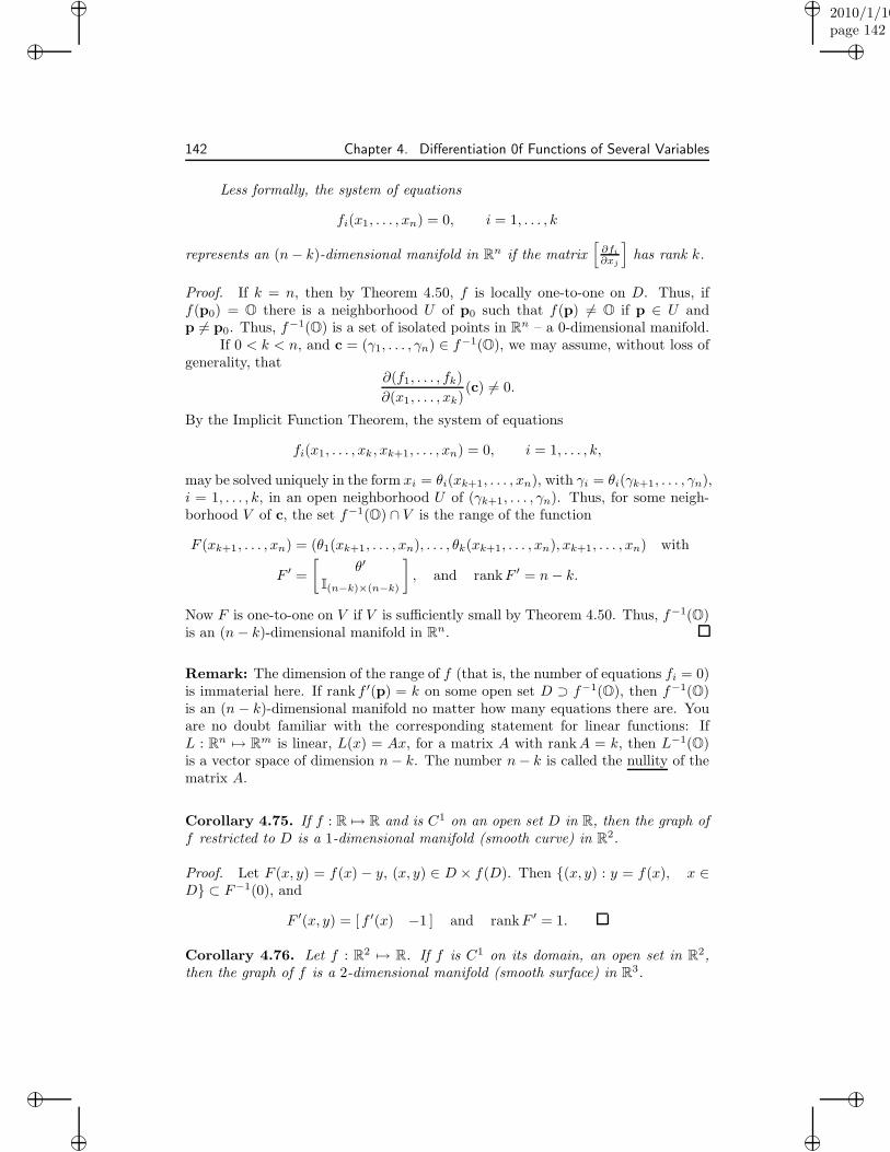
“muldowney”2010/1/10page 142
i
i
i
i
i
i
i
i
142 Chapter 4. Differentiation 0f Functions of Several Variables
Less formally, the system of equations
fi(x1, . . . , xn) = 0, i = 1, . . . , k
represents an (n− k)-dimensional manifold in Rn if the matrix[∂fi
∂xj
]has rank k.
Proof. If k = n, then by Theorem 4.50, f is locally one-to-one on D. Thus, iff(p0) = O there is a neighborhood U of p0 such that f(p) 6= O if p ∈ U andp 6= p0. Thus, f−1(O) is a set of isolated points in Rn – a 0-dimensional manifold.
If 0 < k < n, and c = (γ1, . . . , γn) ∈ f−1(O), we may assume, without loss ofgenerality, that
∂(f1, . . . , fk)
∂(x1, . . . , xk)(c) 6= 0.
By the Implicit Function Theorem, the system of equations
fi(x1, . . . , xk, xk+1, . . . , xn) = 0, i = 1, . . . , k,
may be solved uniquely in the form xi = θi(xk+1, . . . , xn), with γi = θi(γk+1, . . . , γn),i = 1, . . . , k, in an open neighborhood U of (γk+1, . . . , γn). Thus, for some neigh-borhood V of c, the set f−1(O) ∩ V is the range of the function
F (xk+1, . . . , xn) = (θ1(xk+1, . . . , xn), . . . , θk(xk+1, . . . , xn), xk+1, . . . , xn) with
F ′ =
[θ′
I(n−k)×(n−k)
], and rankF ′ = n− k.
Now F is one-to-one on V if V is sufficiently small by Theorem 4.50. Thus, f−1(O)is an (n− k)-dimensional manifold in Rn.
Remark: The dimension of the range of f (that is, the number of equations fi = 0)is immaterial here. If rank f ′(p) = k on some open set D ⊃ f−1(O), then f−1(O)is an (n − k)-dimensional manifold no matter how many equations there are. Youare no doubt familiar with the corresponding statement for linear functions: IfL : Rn 7→ Rm is linear, L(x) = Ax, for a matrix A with rankA = k, then L−1(O)is a vector space of dimension n− k. The number n− k is called the nullity of thematrix A.
Corollary 4.75. If f : R 7→ R and is C1 on an open set D in R, then the graph off restricted to D is a 1-dimensional manifold (smooth curve) in R2.
Proof. Let F (x, y) = f(x) − y, (x, y) ∈ D × f(D). Then {(x, y) : y = f(x), x ∈D} ⊂ F−1(0), and
F ′(x, y) = [ f ′(x) −1 ] and rankF ′ = 1.
Corollary 4.76. Let f : R2 7→ R. If f is C1 on its domain, an open set in R2,then the graph of f is a 2-dimensional manifold (smooth surface) in R3.
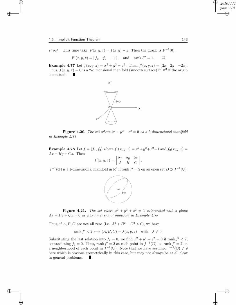
“muldowney”2010/1/10page 143
i
i
i
i
i
i
i
i
4.5. Implicit Function Theorem 143
Proof. This time take, F (x, y, z) = f(x, y)− z. Then the graph is F−1(0),
F ′(x, y, z) = [ fx fy −1 ] , and rankF ′ = 1.
Example 4.77 Let f(x, y, z) = x2 + y2 − z2. Then f ′(x, y, z) = [ 2x 2y −2z ].Thus, f(x, y, z) = 0 is a 2-dimensional manifold (smooth surface) in R3 if the originis omitted.
f=0
x
y
z
0
Figure 4.20. The set where x2 + y2− z2 = 0 as a 2-dimensional manifoldin Example 4.77
Example 4.78 Let f = (f1, f2) where f1(x, y, z) = x2+y2+z2−1 and f2(x, y, z) =Ax+By + Cz. Then
f ′(x, y, z) =
[2x 2y 2zA B C
].
f−1(O) is a 1-dimensional manifold in R3 if rank f ′ = 2 on an open setD ⊃ f−1(O).
����f=0
0
Figure 4.21. The set where x2 + y2 + z2 = 1 intersected with a planeAx+By + Cz = 0 as a 1-dimensional manifold in Example 4.78
Thus, if A,B,C are not all zero (i.e. A2 +B2 + C2 > 0), we have
rank f ′ < 2⇐⇒ (A,B,C) = λ(x, y, z) with λ 6= 0.
Substituting the last relation into f2 = 0, we find x2 + y2 + z2 = 0 if rank f ′ < 2,contradicting f1 = 0. Thus, rank f ′ = 2 at each point in f−1(O), so rank f ′ = 2 ona neighborhood of each point in f−1(O). Note that we have assumed f−1(O) 6= ∅here which is obvious geometrically in this case, but may not always be at all clearin general problems.
“muldowney”2010/1/10page 144
i
i
i
i
i
i
i
i
144 Chapter 4. Differentiation 0f Functions of Several Variables
Question: Let
A(x) =
[a(x) b(x) c(x)d(x) e(x) f(x)
].
Does rankA(x0) = 2 imply that rankA(x) = 2 near x0 if the entries in A arecontinuous? Does rankA(x0) = 1 imply rankA(x) = 1 near x0?
Theorem 4.79. Let D ⊂ Rn be open. Suppose
(i) f : D 7→ Rn and f ∈ C1(D),
(ii) rank f ′(p) = k for every p ∈ D.
Then for each c ∈ D, there is a neighborhood Uc of c such that f(Uc) is a k-dimensional segment.
This theorem is analogous to the statement that the dimension of the rangeof any linear function L(x) = Ax is the rank of A. The proof of this theorem isnotationally quite complicated so we will consider a few examples and special casesfirst. Actually, all the essential ideas of the proof are contained in the special casesso you may skip the proof if you wish.
Example 4.80 Let f : R2 7→ R2 be defined by f(x, y) = (x+ y, (x+ y)2). Then
rank f ′(x, y) = rank
[1 1
2(x+ y) 2(x+ y)
]= 1 ∀ (x, y).
Thus, f(R2) is the 1-dimensional segment {(t, t2) : t ∈ R}, a parabola. We haveused t = x+ y to parameterize the curve.
Example 4.81 Let f : R3 7→ R3 be defined by
f(x, y, z) = (x− y, y − z, x(x− 2y)− z(z − 2y)).
Then
rankf ′(x, y, z) = rank
1 −1 00 1 −1
2(x− y) 2(z − x) 2(y − z)
= 2.
Here f(R3) is the 2-dimensional segment {(u, v, u2−v2) : (u, v) ∈ R2} (a hyperboloidw = u2 − v2) in R3. We used (u, v) = (x − y, y − z) to parameterize the surface.
Proposition 4.82. Let f : R2 7→ R2, and f ∈ C1(D), D open in R2. Ifrankf ′(p) = 1 for every p ∈ D, and u = f1(x, y), v = f2(x, y), then in a neighbor-hood of any point (x0, y0) ∈ D,
either u = φ(v) or v = ψ(u), φ, ψ ∈ C1,
that is, f(D) is composed of 1-dimensional segments.
“muldowney”2010/1/10page 145
i
i
i
i
i
i
i
i
4.5. Implicit Function Theorem 145
Proof. If(∂f1/∂x
)(x0, y0) 6= 0, then ∂f1/∂x 6= 0 in an open neighborhood U of
(x0, y0), so f1(U) is open (Theorem 4.53). By the Implicit Function Theorem, near(x0, y0, u0), the equation u = f1(x, y) may be solved uniquely for x in the form
x = θ(u, y), with θ ∈ C1 =⇒ v = f2(θ(u, y), y).
We show that the last equation is independent of y:
∂v
∂y=∂f2∂x
∂θ
∂y+∂f2∂y
=∂f2∂x
(−∂f1∂y∂f1∂x
)+∂f2∂y
=
∂f1∂x
∂f2∂y −
∂f2∂x
∂f1∂y
∂f1∂x
=
∂(f1,f2)∂(x,y)
∂f1∂x
= 0,
since rank f ′ = 1. Thus, v = φ(u); that is, we have a local parameterization off(U0) in the form
f(U0) = {(u, φ(u)) : u ∈ f1(U0)} ,where U0 is an open neighborhood of (x0, y0).
Proposition 4.83. Let f : R3 7→ R3 and f ∈ C1(D) for an open set D ⊂ R3. Ifrank f ′(p) = 2 for all p ∈ D and
u = f1(x, y, z), v = f2(x, y, z), w = f3(x, y, z),
then in some neighborhood U of each point (x0, y0, z0) ∈ D,
either w = φ(u, v), or u = ψ(v, w), or v = η(w, u), φ, ψ, η ∈ C1,
that is, f(U) is a 2-dimensional segment in R3.
Proof. From the Implicit Function Theorem,
∂(f1, f2)
∂(x, y)(x0, y0, z0) 6= 0 =⇒ u = f1(x, y, z) and v = f2(x, y, z),
are uniquely solvable for (x, y) in the form
x = θ1(u, v, z), y = θ2(u, v, z), θ1, θ2 ∈ C1;
hence
w = f3(θ1(u, v, z), θ2(u, v, z), z).
We observe that this last function is actually independent of z:
∂w
∂z=∂f3∂x
∂θ1∂z
+∂f3∂y
∂θ2∂z
+∂f3∂z
“muldowney”2010/1/10page 146
i
i
i
i
i
i
i
i
146 Chapter 4. Differentiation 0f Functions of Several Variables
=∂f3∂x
−
∂(f1,f2)∂(z,y)
∂(f1,f2)∂(x,y)
+
∂f3∂y
−
∂(f1,f2)∂(x,z)
∂(f1,f2)∂(x,y)
+
∂f3∂z
=
(∂f3∂x
∂(f1,f2)∂(y,z) −
∂f3∂y
∂(f1,f2)∂(x,z) + ∂f3
∂z∂(f1,f2)∂(x,y)
)
∂(f1,f2)∂(x,y)
=
∂(f1,f2,f3)∂(x,y,z)
∂(f1,f2)∂(x,y)
= 0, since rank f ′ = 2.
Therefore,
w = φ(u, v) and f(U0) = {(u, v, φ(u, v)) : (u, v) ∈ (f1, f2)(U0)},for some open neighborhood U0 of (x0, y0, z0).
Proof of Theorem 4.79. (Optional) If k = n, then f is locally one-to-one (Theorem4.50) so the theorem reduces to the definition of a k-dimensional segment. If k = 0,then
∂fi∂xj
= 0, ∀ i, j =⇒ f is constant
in a convex neighborhood U of c, thus f(U) = {f(c)} which is a 0-dimensionalsegment.
When 0 < k < n, consider
ui = fi(x1, . . . , xn), i = 1, . . . , n. (4.34)
We are given that rank f ′(p) = k. So if c ∈ D and if (say)
∂(f1, . . . , fk)
∂(x1, . . . , xk)(p) 6= 0 at p = c, (4.35)
then (4.35) also holds in an open neighborhood U of c since f ∈ C1(D). Therefore,the set
V = (f1, . . . , fk)(U) ⊂ Rk is open in Rk
by Lemma 4.52. By the Implicit Function Theorem, condition (4.35) implies thatthe first k equations in (4.34) may be solved for (x1, . . . , xk) in the form
xi = θi(u1, . . . , uk, xk+1, . . . , xn), i = 1, . . . , k. (4.36)
Substituting (4.36) into the remaining (n− k) equations in (4.34) yields
ui = fi(θ1, . . . , θk, xk+1, . . . , xn), i = k + 1, . . . , n. (4.37)
We claim that these are functions of (u1, . . . , un) only. We show only that there isno dependence on xk+1. By the derivative formula (4.31) of the Implicit FunctionTheorem,
∂θℓ∂xk+1
= −∂(f1,...,fk)
∂(x1,...,xℓ−1,xk+1,xℓ+1,...,xk)
∂(f1,...,fk)∂(x1,...,xk)
, ℓ = 1, . . . , k.
“muldowney”2010/1/10page 147
i
i
i
i
i
i
i
i
4.5. Implicit Function Theorem 147
Substituting these into the Chain Rule applied to equations from (4.37), using theeffect of interchanging rows in determinants, and using the expansion of a determi-nant about row i, we obtain
∂ui∂xk+1
=
k∑
ℓ=1
∂fi∂xℓ
−
∂(f1,...,fk)∂(x1,...,xℓ−1,xk+1,xℓ+1,...,xk)
(f1,...,fk)∂(x1,...,xk)
+
∂fi∂xk+1
=
k+1∑
ℓ=1
(−1)k+1−ℓ ∂fi∂xℓ
∂(f1,...,fk)∂(x1,...,xℓ−1,xℓ+1,...,xk,xk+1)
∂(f1,...,fk)∂(x1,...,xk)
=
∂(f1,...,fk,fi)∂(x1,...,xk+1)
∂(f1,...,fk)∂(x1,...,xk)
= 0, since rank f ′ = k.
Thus, (4.37) may be written in the form
ui − φ(u1, . . . , uk) = 0, i = k + 1, . . . , n, with φi ∈ C1(V0) (4.38)
where V0 = (f1, . . . , fk)(U0) is open. The Jacobian matrix of the (n− k) equations(4.38) is the (n− k)× k matrix of the form
[ I(n−k)×(n−k) φ′ ]
which has rank (n − k). Therefore, by Theorem 4.74, is a k-dimensional manifold.
[Notice that the pen never left the hand!!]
4.5.2 Application: Lagrange Multipliers
Here we provide an application of the Implicit Function Theorem to extremal prob-lems subject to constraints.
Definition 4.84. Let f : D ⊂ Rn 7→ R be a real-valued function on the domain D.The function f has a relative maximum (respectively, minimum) with respect to a setS at p0 ∈ S ∩D if, for some neighborhood U of p0
f(p) ≤ f(p0) ∀ p ∈ S ∩ U (respectively, f(p) ≥ f(p0) ∀ p ∈ S ∩ U).
Theorem 4.85 (Lagrange Multiplier Rule). Let f : Rn 7→ R and g =g1, . . . , gk) : Rn 7→ Rk, k < n. If f and g are C1 functions near p0 and
(i) f has a relative extrema at p0 with respect to the set
S = g−1(O) = {p : gi(p) = 0, i = 1, . . . , k},
(ii) rank g′(p0) = k,
“muldowney”2010/1/10page 148
i
i
i
i
i
i
i
i
148 Chapter 4. Differentiation 0f Functions of Several Variables
then there exists real numbers λ1, . . . , λk such that
∂f
∂xi(p0) +
k∑
j=1
λj∂gj∂xi
(p0) = 0, i = 1, . . . , n.
The equations gi(p) = 0, i = 1, . . . , k are called constraints. The numbers λiare called Lagrange multipliers.
Before we give a couple of proofs of this theorem, we give some applications.
Example 4.86 Find the distance d from the point (0, 0) to the line x+y = 1. Theproblem is to minimize x2 + y2 subject to the constrain x+ y−1 = 0. We note thata minimum exists since x2 + y2 goes to infinity as |(x, y)| → ∞ and that x2 + y2 isnon-negative. At the minimum value, the Lagrange Multiplier Rule says that thereis a λ such that
2x+ λ = 0, 2y + λ = 0, with x+ y − 1 = 0.
Solving this linear system of equations for (x, y, λ) we find
(x, y, λ) = (1
2,1
2,−1) =⇒ d2 =
(1
2
)2
+
(1
2
)2
=1
2, or d =
1√2.
Example 4.87 Find the maximum and minimum of f(x, y) = 2x2 − 3y2 − 2x inthe set {(x, y) : x2 + y2 ≤ 1}.
If either the max or min occur in the open set {(x, y) : x2 + y2 < 1}, then
∂f∂x = 4x− 2 = 0∂f∂y = −6y = 0
}=⇒ (x, y) =
(1
2, 0
).
But, [fxx fxyfyx fyy
]=
[4 00 −6
]is indefinite,
so f has a saddle point at (12 , 0). Therefore, the maximum and minimum occur in
the set
{(x, y) : x2 + y2 − 1 = 0}.The Lagrange Multiplier Rule then gives the existence of a λ such that at theextrema
4x− 2 + 2λx = 0
−6y + 2λy = 0
x2 + y2 − 1 = 0.
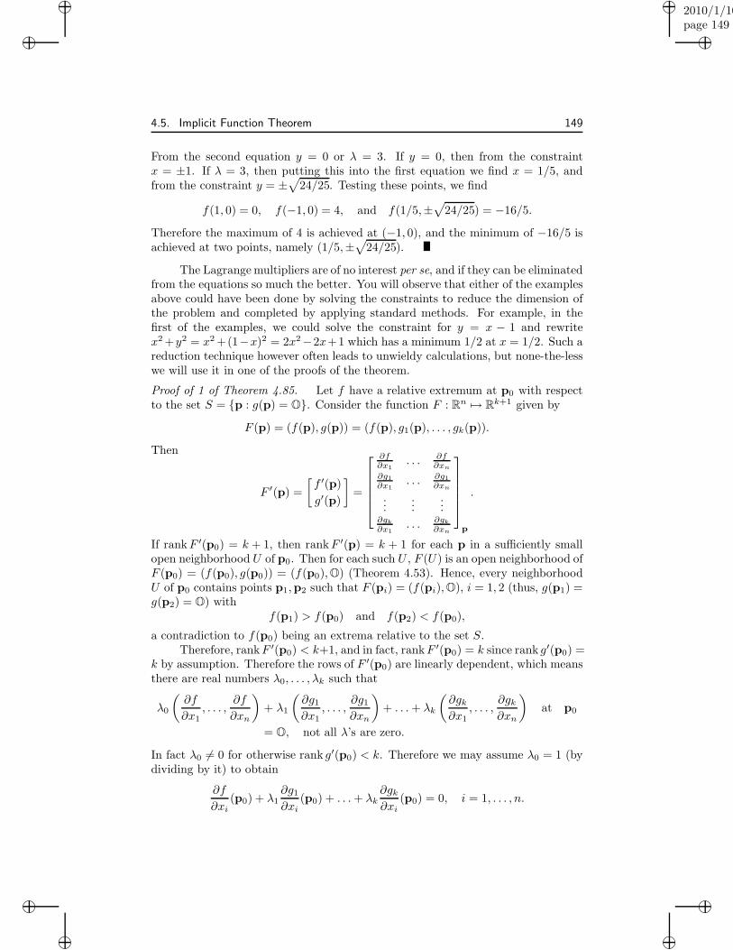
“muldowney”2010/1/10page 149
i
i
i
i
i
i
i
i
4.5. Implicit Function Theorem 149
From the second equation y = 0 or λ = 3. If y = 0, then from the constraintx = ±1. If λ = 3, then putting this into the first equation we find x = 1/5, andfrom the constraint y = ±
√24/25. Testing these points, we find
f(1, 0) = 0, f(−1, 0) = 4, and f(1/5,±√
24/25) = −16/5.
Therefore the maximum of 4 is achieved at (−1, 0), and the minimum of −16/5 isachieved at two points, namely (1/5,±
√24/25).
The Lagrange multipliers are of no interest per se, and if they can be eliminatedfrom the equations so much the better. You will observe that either of the examplesabove could have been done by solving the constraints to reduce the dimension ofthe problem and completed by applying standard methods. For example, in thefirst of the examples, we could solve the constraint for y = x − 1 and rewritex2 +y2 = x2 +(1−x)2 = 2x2−2x+1 which has a minimum 1/2 at x = 1/2. Such areduction technique however often leads to unwieldy calculations, but none-the-lesswe will use it in one of the proofs of the theorem.
Proof of 1 of Theorem 4.85. Let f have a relative extremum at p0 with respectto the set S = {p : g(p) = O}. Consider the function F : Rn 7→ Rk+1 given by
F (p) = (f(p), g(p)) = (f(p), g1(p), . . . , gk(p)).
Then
F ′(p) =
[f ′(p)
g′(p)
]=
∂f∂x1
. . . ∂f∂xn
∂g1∂x1
. . . ∂g1∂xn
......
...∂gk
∂x1. . . ∂gk
∂xn
p
.
If rankF ′(p0) = k + 1, then rankF ′(p) = k + 1 for each p in a sufficiently smallopen neighborhood U of p0. Then for each such U , F (U) is an open neighborhood ofF (p0) = (f(p0), g(p0)) = (f(p0),O) (Theorem 4.53). Hence, every neighborhoodU of p0 contains points p1,p2 such that F (pi) = (f(pi),O), i = 1, 2 (thus, g(p1) =g(p2) = O) with
f(p1) > f(p0) and f(p2) < f(p0),
a contradiction to f(p0) being an extrema relative to the set S.Therefore, rankF ′(p0) < k+1, and in fact, rankF ′(p0) = k since rank g′(p0) =
k by assumption. Therefore the rows of F ′(p0) are linearly dependent, which meansthere are real numbers λ0, . . . , λk such that
λ0
(∂f
∂x1, . . . ,
∂f
∂xn
)+ λ1
(∂g1∂x1
, . . . ,∂g1∂xn
)+ . . .+ λk
(∂gk∂x1
, . . . ,∂gk∂xn
)at p0
= O, not all λ’s are zero.
In fact λ0 6= 0 for otherwise rank g′(p0) < k. Therefore we may assume λ0 = 1 (bydividing by it) to obtain
∂f
∂xi(p0) + λ1
∂g1∂xi
(p0) + . . .+ λk∂gk∂xi
(p0) = 0, i = 1, . . . , n.
“muldowney”2010/1/10page 150
i
i
i
i
i
i
i
i
150 Chapter 4. Differentiation 0f Functions of Several Variables
Rn
g(p)=0
p0
UF(U)
(f(p ),0)R
Rk
F
S:0
Figure 4.22. Every neighborhood U of p0 contains points p1,p2 such thatF (pi) = (f(pi),O), i = 1, 2
These n equations together with the k constraint equations
gj(p0) = 0, j = 1, . . . , k,
serve to determine the (n + k) numbers which are the coordinates of p0 and theλ1, . . . , λk.
Proof of 2 of Theorem 4.85. This proof works in general but we prove just thecase of one constraint. Suppose f, g : Rn 7→ R are C1 functions and f(p), p =(x1, . . . , xn), has an extremum at c = (γ1, . . . , γn), with respect to the constraint
g(p) = 0. (4.39)
If rank g′(c) = 1, then we may assume that (∂g/∂x1)(c) 6= 0. Then, equation (4.39)may be solved for x1 in a neighborhood of (γ2, . . . , γn) in the form
x1 = φ(x2, . . . , xn), with φ ∈ C1 and γ1 = φ(γ2, . . . , γn).
Therefore, f(φ(x2, . . . , xn), x2, . . . , xn) has an interior relative extremum at c =(γ2, . . . , γn). Hence all of its partial derivative vanish at c; so by the Chain Rule
∂f
∂xi(c) +
∂f
∂x1(c)
∂φ
∂xi(c) = 0, i = 2, . . . , n, or
∂f
∂xi(c) +
∂f
∂x1(c)
(−
∂g∂xi
(c)∂g∂x1
(c)
)= 0, i = 2, . . . , n.
The last equation holds trivially for i = 1 as well. Hence we find
∂f
∂xi(c) + λ
∂g
∂xi(c) = 0, i = 1, . . . , n with λ = −
∂f∂x1
∂g∂x1
.
Exercises
4.77. Let f(x, y) = (x+ y, 2x+ ay) = (u, v).
“muldowney”2010/1/10page 151
i
i
i
i
i
i
i
i
4.5. Implicit Function Theorem 151
(i) Show that rank f ′(x, y) = 2 if and only if a 6= 2.
(ii) Find the image of the square
K := {(x, y) : 0 ≤ x ≤ 1, 0 ≤ y ≤ 1}
in the three cases a = 1, a = 2, a = 3.
(iii) If a point moves around the boundary of K in the counterclockwisesense, find what its image does in the cases a = 1, a = 3. What is thesign of Jf in each case?
4.78. Let f(x, y) = (x, xy) = (u, v). Draw some curves u = constant, v = constantin the (x, y) plane and some curves x = constant, y = constant in the (u, v)plane. Is this map one-to-one? Into what region of the (u, v) plane does fmap the rectangle {(x, y) : 1 ≤ x ≤ 2, 0 ≤ y ≤ 2}? What points in the(x, y) plane map into the rectangle {(u, v) : 1 ≤ u ≤ 2, 0 ≤ v ≤ 2}?
4.79. If f(x, y) = (cos(x + y), sin(x + y)) = (u, v), show from f ′(x, y) that (u, v)lies on a curve in the (u, v) plane. What is its equation?
4.80. In each of the following show that (u, v, w) lies on a surface in R3 and findan equation for the surface.
(i) u = x+yz , v = z+y
x , w = y(x+y+z)xz .
(ii) u = x+ y + z, v = xy + yz + zx, w = x3 + y3 + z3 − 3xyz.
(iii) u = x+ y + z, v = x2 + y2 + z2, w = x3 + y3 + z3 − 3xyz.
[Solutions: (i) w + 1 = uv, (ii) w = u(u2 − 3v), (iii) w = u(3v − u2)/2.]
4.81. Show that {(u cos(v), u sin(v), u) : 0 < u < 1, 0 < v < 2π} is a 2-dimensional segment in R3. Draw a picture of it.
4.82. Show that a set cannot be both an r-dimensional segment and a k-dimensionalsegment if r 6= k. [Hint: Suppose S = φ(U) = ψ(V ) where φ, ψ are C1
functions on U, V respectively, U, V are open sets in Rr, Rk respectively with(say) r < k. Show that if φ and ψ are one-to-one and rankφ′ = r, rankψ′ = k,there is a contradiction. Use the Implicit Function Theorem.]
4.83. If φi, i = 1, . . . , k are C1 functions on an open set D ⊂ Rn, then the set ofpoints (x1, . . . , xn, y1, . . . , yk) in Rn+k satisfying
yi = φi(x1, . . . , xn), i = 1, . . . , k
is an n-dimensional manifold in Rn+k. [That is, the graph of a C1 functionfrom Rn 7→ Rk is an n-dimensional manifold if its domain is open.]
4.84. Let V = x2 + y2 + z2, φ = x2 + y2 − 1, ψ = x + y + z. Find themaximum and minimum of V subject to the constraints φ = 0, ψ = 0.This means: “Find the length (squared) of the major and minor semi-axesof the ellipse C which is the intersection of the cylinder φ = 0 and theplane ψ = 0”. [Solution: maxV = V (±(−1/
√2,−1/
√2,√
2)) = 3 andmin V = V (±(1/
√2,−1/
√2, 0)) = 1.]
4.85. Find the minimum value of V = x2 + y2 + z2 when
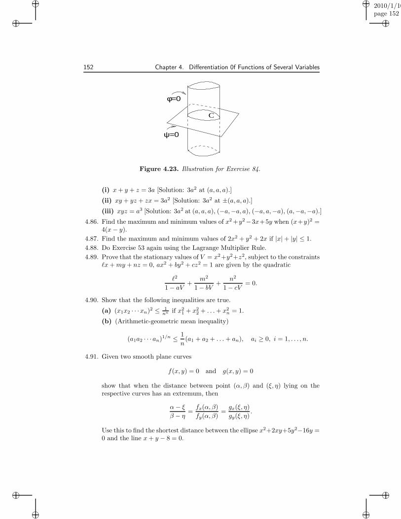
“muldowney”2010/1/10page 152
i
i
i
i
i
i
i
i
152 Chapter 4. Differentiation 0f Functions of Several Variables
C
φ=0
ψ=0
Figure 4.23. Illustration for Exercise 84.
(i) x+ y + z = 3a [Solution: 3a2 at (a, a, a).]
(ii) xy + yz + zx = 3a2 [Solution: 3a2 at ±(a, a, a).]
(iii) xyz = a3 [Solution: 3a2 at (a, a, a), (−a,−a, a), (−a, a,−a), (a,−a,−a).]4.86. Find the maximum and minimum values of x2 +y2−3x+5y when (x+y)2 =
4(x− y).4.87. Find the maximum and minimum values of 2x2 + y2 + 2x if |x|+ |y| ≤ 1.
4.88. Do Exercise 53 again using the Lagrange Multiplier Rule.
4.89. Prove that the stationary values of V = x2+y2+z2, subject to the constraintsℓx+my + nz = 0, ax2 + by2 + cz2 = 1 are given by the quadratic
ℓ2
1− aV +m2
1− bV +n2
1− cV = 0.
4.90. Show that the following inequalities are true.
(a) (x1x2 · · ·xn)2 ≤ 1nn if x2
1 + x22 + . . .+ x2
n = 1.
(b) (Arithmetic-geometric mean inequality)
(a1a2 · · · an)1/n ≤1
n(a1 + a2 + . . .+ an), ai ≥ 0, i = 1, . . . , n.
4.91. Given two smooth plane curves
f(x, y) = 0 and g(x, y) = 0
show that when the distance between point (α, β) and (ξ, η) lying on therespective curves has an extremum, then
α− ξβ − η =
fx(α, β)
fy(α, β)=gx(ξ, η)
gy(ξ, η).
Use this to find the shortest distance between the ellipse x2+2xy+5y2−16y =0 and the line x+ y − 8 = 0.
“muldowney”2010/1/10page 153
i
i
i
i
i
i
i
i
4.5. Implicit Function Theorem 153
4.92. Let f be a real valued function of class C1 on R3. Prove that there are at leasttwo points on the sphere x2 + y2 + z2 = R2, R > 0, at which the equations
y∂f
∂x− x∂f
∂y= 0
z∂f
∂y− y ∂f
∂z= 0
x∂f
∂z− z ∂f
∂x= 0
are satisfied.
4.93. (The Holder and Minkowski inequalities.) Let p > 1, q > 1 and 1p + 1
q = 1.
(a) Show that the minimum of f(x, y) = xp
p + yq
q subject to the constraintsx > 0, y > 0, and xy = 1 is 1.
(b) Show that a ≥ 0, b ≥ 0 implies ab ≤ ap
p + bq
q .
(c) Show that ak ≥ 0, bk ≥ 0, k = 1, . . . , n implies
n∑
k=1
akbk ≤(
n∑
k=1
apk
)1/p( n∑
k=1
bqk
)1/q
(Holder’s Inequality).
[Hint: Let A = (∑n
k=1 apk)
1/pand B = (
∑nk=1 b
qk)
1/qand consider a =
ak/A, b = bk/B.]
(d) If ak, bk, k = 1, . . . , n are real numbers and p ≥ 1, then
(n∑
k=1
|ak + bk|p)1/p
≤(
n∑
k=1
|ak|p)1/p
+
(n∑
k=1
|bk|p)1/p
.
(Minkowski’s inequality) [Hint: |a + b|p = |a + b||a + b|p/q ≤ |a||a +b|p/q + |b||a+ b|p/q if p > 1. Use Holder’s inequality.]
References for Chapter IV
R. G. Bartle: Chapter V.
R. C. Buck: Chapter V.
“muldowney”2010/1/10page 154
i
i
i
i
i
i
i
i
154 Chapter 4. Differentiation 0f Functions of Several Variables
“muldowney”2010/1/10page 155
i
i
i
i
i
i
i
i
Chapter 5
Further Topics inIntegration
5.1 Changes of Variables in Integrals
Every n× n matrix A can be expressed as a product of a finite number of matricesof the (block) form
A1 =
I O O
O a O
O O I
← k-row
A2 =
I O O O O
O 1 O 1 O
O O I O O
O 0 O 1 O
O O O O I
← k-row
← j-row
A3 =
I O O O O
O 0 O 1 O
O O I O O
O 1 O 0 O
O O O O I
.← k-row
← j-row
That is, every linear function from Rn to Rn can be expressed as a composition oflinear functions of the form
L1(x1, . . . , xk−1, xk, xk+1, . . . , xn) = (x1, . . . , xk−1, axk, xk+1, . . . , xn)
L2(x1, . . . , xk−1, xk, xk+1, . . . , xn) = (x1, . . . , xk−1, xk + xj , xk+1, . . . , xn)
L3(x1, . . . , xk−1, xk, . . . , xj−1, xj . . . , xn) = (x1, . . . , xk−1, xj , . . . , xj−1, xk, . . . , xn)
We shall not prove this statement. You should prove it yourself as an exercise; itis obviously true for n = 1, use induction on n. But first prove it for n = 2 to seehow the general proof should go.
155
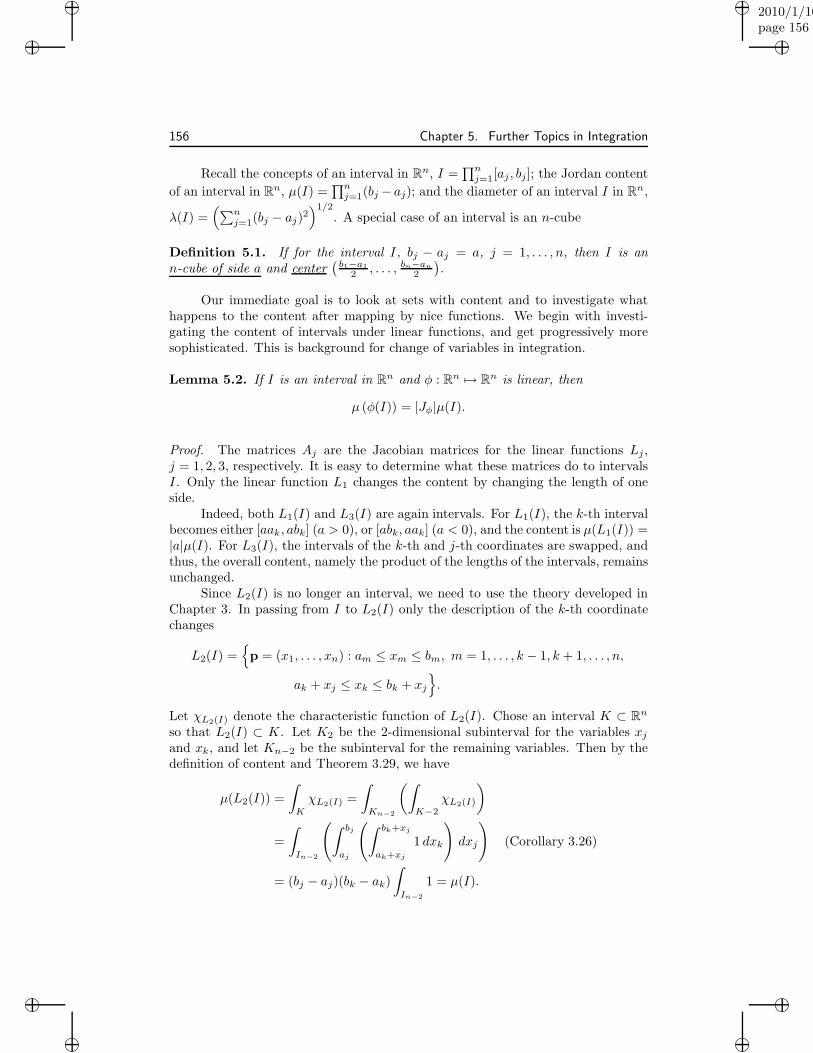
“muldowney”2010/1/10page 156
i
i
i
i
i
i
i
i
156 Chapter 5. Further Topics in Integration
Recall the concepts of an interval in Rn, I =∏nj=1[aj , bj]; the Jordan content
of an interval in Rn, µ(I) =∏nj=1(bj − aj); and the diameter of an interval I in Rn,
λ(I) =(∑n
j=1(bj − aj)2)1/2
. A special case of an interval is an n-cube
Definition 5.1. If for the interval I, bj − aj = a, j = 1, . . . , n, then I is ann-cube of side a and center
(b1−a1
2 , . . . , bn−an
2
).
Our immediate goal is to look at sets with content and to investigate whathappens to the content after mapping by nice functions. We begin with investi-gating the content of intervals under linear functions, and get progressively moresophisticated. This is background for change of variables in integration.
Lemma 5.2. If I is an interval in Rn and φ : Rn 7→ Rn is linear, then
µ (φ(I)) = |Jφ|µ(I).
Proof. The matrices Aj are the Jacobian matrices for the linear functions Lj ,j = 1, 2, 3, respectively. It is easy to determine what these matrices do to intervalsI. Only the linear function L1 changes the content by changing the length of oneside.
Indeed, both L1(I) and L3(I) are again intervals. For L1(I), the k-th intervalbecomes either [aak, abk] (a > 0), or [abk, aak] (a < 0), and the content is µ(L1(I)) =|a|µ(I). For L3(I), the intervals of the k-th and j-th coordinates are swapped, andthus, the overall content, namely the product of the lengths of the intervals, remainsunchanged.
Since L2(I) is no longer an interval, we need to use the theory developed inChapter 3. In passing from I to L2(I) only the description of the k-th coordinatechanges
L2(I) ={p = (x1, . . . , xn) : am ≤ xm ≤ bm, m = 1, . . . , k − 1, k + 1, . . . , n,
ak + xj ≤ xk ≤ bk + xj
}.
Let χL2(I) denote the characteristic function of L2(I). Chose an interval K ⊂ Rn
so that L2(I) ⊂ K. Let K2 be the 2-dimensional subinterval for the variables xjand xk, and let Kn−2 be the subinterval for the remaining variables. Then by thedefinition of content and Theorem 3.29, we have
µ(L2(I)) =
∫
K
χL2(I) =
∫
Kn−2
(∫
K−2
χL2(I)
)
=
∫
In−2
(∫ bj
aj
(∫ bk+xj
ak+xj
1 dxk
)dxj
)(Corollary 3.26)
= (bj − aj)(bk − ak)∫
In−2
1 = µ(I).
“muldowney”2010/1/10page 157
i
i
i
i
i
i
i
i
5.1. Changes of Variables in Integrals 157
Thus, the Lemma holds for the elementary linear functions. Since any linearfunction is a composition of finitely many elementary linear functions, the differen-tial is the product of the differentials, and hence the Jacobian is the product of theJacobians, the general case follows.
The next three lemmas and Theorem 5.7 that follows are technical in nature.In view of the last lemma, you will find it easy to accept Theorem 5.7, so on yourfirst reading, you may proceed directly to the important change of variables theorem,Theorem 5.8; however, read the statement of Theorem 5.7 first.
Lemma 5.3. Suppose that φ : G ⊂ Rn 7→ Rn, is C1(G) on the open set G. Then
D ⊂ G, D compact and µ(D) = 0 =⇒ µ(φ(D)) = 0.
In particular, this holds if φ is a linear map of rank n.
Proof. If ǫ > 0, there is a finite collection of n-cubes Ij , j = 1, . . . ,m, such that
D ⊂ ∪mj=1Ij ⊂ G and∑m
j=1 µ(Ij) < ǫ (Why?)
φ ∈ C1(G) =⇒ φ ∈ C1(∪mj=1Ij
).
Thus, the partial derivatives of φ are continuous on the compact set ∪mj=1Ij . There-fore, there exists M > 0 such that
|Dφ(p)(u)| ≤M |u|, ∀ p ∈ ∪mj=1Ij , ∀ u ∈ Rn.
From the Mean Value Theorem 4.29 applied to φ, we find
|φ(p)− φ(q)| ≤M |p− q|, ∀ p,q ∈ Ij , j = 1, . . . ,m,
≤Mλ(Ij) =√nMµ(Ij)
1/n, (Ij is an n-cube).
Therefore, the diameter of φ(Ij) is at most√nMµ(Ij)
1/n, and so we can find ann-cube Kj with
φ(Ij) ⊂ Kj and µ(Kj) ≤(2√nM
)nµ(Ij), j = 1, . . . ,m.
Consequently,
φ(D) ⊂ ∪nj=1Kj and µ(φ(D) ≤n∑
j=1
µ(Kj) ≤(2√nM
)nǫ.
It follows that φ(D) has content zero.
Lemma 5.4. Suppose G ⊂ Rn is an open set and φ : G 7→ Rn satisfies
φ ∈ C1(G) and Jφ(p) 6= 0, ∀ p ∈ G.
“muldowney”2010/1/10page 158
i
i
i
i
i
i
i
i
158 Chapter 5. Further Topics in Integration
If D is a compact subset of G and D has content, then φ(D) is a compact set withcontent.
Proof. We know that φ ∈ C(D) andD compact implies φ(D) is compact (Theorem2.36). In particular, ∂D ⊂ D implies that the boundary of φ(D) is contained inφ(D). By Theorem 4.50 and Theorem 4.53, φ is locally one-to-one on G and mapsopen sets onto open sets. Therefore,
both φ(G) and φ(G)\φ(D) are open sets.
Now, if φ(p) = q is on the boundary of φ(D), then each neighborhood V of qcontains a point q1 ∈ φ(G)\φ(D), which implies that each neighborhood U of pcontains a point in G\D. Therefore, p is in the boundary of D and we have shown
∂(φ(D)) ⊂ φ(∂(D)). (5.1)
The set D has content if and only if the content of its boundary is zero (The-orem 3.14). Therefore
µ(∂D) = 0 =⇒ µ(φ(∂(D))) = 0, Lemma 5.3
=⇒ µ(∂(φ(D))) = 0, by (5.1)
=⇒ φ(D) has content. (Theorem 3.14)
Lemma 5.5. Suppose that K is the n-cube of side 2r centered at O, i.e
K = [−r, r]× . . .× [−r, r]︸ ︷︷ ︸n times
.
Let G be an open set in Rn containing K and suppose we have a function ψ : G 7→ Rn
such thatψ ∈ C1(G) and Jψ(p) 6= 0, ∀ p ∈ K.
Then for α, 0 < α < 1/√n,
|ψ(p)− p| < α|p|, ∀ p ∈ K =⇒(1− α√n
)n<µ(ψ(K))
µ(K)<(1 + α
√n)n.
Proof. From the proof of Lemma 5.4, (5.1), we know that ∂(ψ(K)) ⊂ ψ(∂(K)). Ifp = (x1, . . . , xn) ∈ ∂(K), then r ≤ |p| ≤ √n r, and consequently,
|ψ(p)− p| < α|p| ≤ α√n r=⇒ r(1 − α√n) ≤︸︷︷︸
some j
|xj | − α√n r ≤ |ψj(p)| ≤ |xj |+ α
√n r ≤ r(1 + α
√n),
where the left most inequality is true for at least one j. Therefore, the boundaryof ψ(K) lies outside an n-cube of side 2(1 − α√n)r with center O and inside ann-cube of side 2(1 + α
√n)r with center O. Since µ(K) = (2r)n, this implies
(1− α√n
)n<µ(ψ(K))
µ(K)<(1 + α
√n)n.
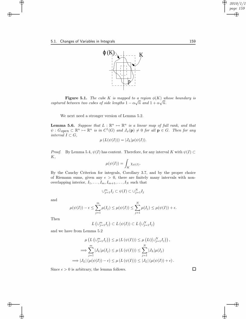
“muldowney”2010/1/10page 159
i
i
i
i
i
i
i
i
5.1. Changes of Variables in Integrals 159
ϕ (K)
p
K
Figure 5.1. The cube K is mapped to a region φ(K) whose boundary iscaptured between two cubes of side lengths 1− α√n and 1 + α
√n.
We next need a stronger version of Lemma 5.2.
Lemma 5.6. Suppose that L : Rn 7→ Rn is a linear map of full rank, and thatψ : Gopen ⊂ Rn 7→ Rn is in C1(G) and Jψ(p) 6= 0 for all p ∈ G. Then for anyinterval I ⊂ G,
µ (L(ψ(I))) = |JL|µ(ψ(I)).
Proof. By Lemma 5.4, ψ(I) has content. Therefore, for any intervalK with ψ(I) ⊂K,
µ(ψ(I)) =
∫
K
χψ(I).
By the Cauchy Criterion for integrals, Corollary 3.7, and by the proper choiceof Riemann sums, given any ǫ > 0, there are finitely many intervals with non-overlapping interior, I1, . . . , Im, Im+1, . . . , IN such that
∪mj=1Ij ⊂ ψ(I) ⊂ ∪Nj=1Ij
and
µ(ψ(I)) − ǫ ≤m∑
j=1
µ(Ij) ≤ µ(ψ(I)) ≤N∑
j=1
µ(Ij) ≤ µ(ψ(I)) + ǫ.
ThenL(∪mj=1Ij
)⊂ L (ψ(I)) ⊂ L
(∪Nj=1Ij
)
and we have from Lemma 5.2
µ(L(∪mj=1Ij
))≤ µ (L (ψ(I))) ≤ µ
(L((∪Nj=1Ij
)),
=⇒m∑
j=1
|JL|µ(Ij) ≤ µ (L (ψ(I))) ≤N∑
j=1
|JL|µ(Ij)
=⇒ |JL| (µ(ψ(I))− ǫ) ≤ µ (L (ψ(I))) ≤ |JL| (µ(ψ(I)) + ǫ) .
Since ǫ > 0 is arbitrary, the lemma follows.
“muldowney”2010/1/10page 160
i
i
i
i
i
i
i
i
160 Chapter 5. Further Topics in Integration
Theorem 5.7 (The Jacobian Theorem). Suppose D is a compact subset of anopen set G ⊂ Rn and
φ : G 7→ Rn, φ ∈ C1(G) with Jφ(p) 6= 0, ∀p ∈ G.
Then, given ǫ > 0, there is a γ(ǫ) > 0 such that for any n-cube, K, with centerp ∈ D and side length less than 2γ,
|Jφ(p)| (1 − ǫ)n ≤ µ(φ(K))
µ(K)≤ |Jφ(p)| (1 + ǫ)n.
Proof. Since Jφ(p) 6= 0, (Dφ(p))−1
=: Lp exists and is linear. Moreover, det[Lp] =1/Jφ(p). Since D is compact and φ ∈ C1(D), the partial derivatives of φ areuniformly continuous on D and we can deduce the following:
(a) There is an M > 0 such that
|Lp(u)| ≤M |u|, ∀p ∈ D and ∀u ∈ Rn. (Why?)
(b) If ǫ > 0 is given, there is a δ = δ(ǫ) > 0 (independent of p) such that
(p ∈ D and |u| < δ) =⇒ |φ(p + u)− φ(p) −Dφ(p)(u)| ≤ ǫ
M√n|u|.
Indeed, for any p + u ∈ B(p, δ) ⊂ G centered on p, by the Mean ValueTheorem (Theorem 4.29), φ(p +u)−φ(p) = Dφ(c)(u) for some c on the linesegment joining p + u and p. The inequality follows for suitable δ by theuniform continuity of the partial derivatives when |p− c| < δ.
For fixed p, define ψ(u) = Lp(φ(p + u)− φ(p)). Then
|ψ(u)− u| = |ψ(u)− Lp(Dφ(p))(u)| ≤ ǫ√n|u|, by (a) and (b).
Applying Lemma 5.5 with α = ǫ/√n to ψ, we find
(1− ǫ)n ≤ µ(ψ(K))
µ(K)≤ (1 + ǫ)n.
But, by Lemma 5.6 applied to φ and K − p where φ(u) = φ(p + u) − φ(p), andfrom the fact that content is invariant under translation, we find
µ(ψ(K)) = µ(Lp(φ(K − p)) = | det[Lp]|µ(φ(K − p))
=µ(φ(K)− φ(p))
|Jφ(p)| =µ(φ(K))
|Jφ(p)|
=⇒ |Jφ(p)| (1− ǫ)n ≤ µ(φ(K))
µ(K)≤ |Jφ(p)| (1 + ǫ)n.
Theorem 5.8 (Change of Variable Theorem). Suppose that
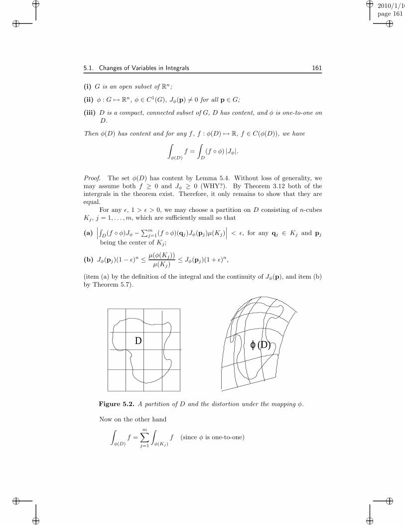
“muldowney”2010/1/10page 161
i
i
i
i
i
i
i
i
5.1. Changes of Variables in Integrals 161
(i) G is an open subset of Rn;
(ii) φ : G 7→ Rn, φ ∈ C1(G), Jφ(p) 6= 0 for all p ∈ G;
(iii) D is a compact, connected subset of G, D has content, and φ is one-to-one onD.
Then φ(D) has content and for any f , f : φ(D) 7→ R, f ∈ C(φ(D)), we have
∫
φ(D)
f =
∫
D
(f ◦ φ) |Jφ|.
Proof. The set φ(D) has content by Lemma 5.4. Without loss of generality, wemay assume both f ≥ 0 and Jφ ≥ 0 (WHY?). By Theorem 3.12 both of theintergrals in the theorem exist. Therefore, it only remains to show that they areequal.
For any ǫ, 1 > ǫ > 0, we may choose a partition on D consisting of n-cubesKj, j = 1, . . . ,m, which are sufficiently small so that
(a)∣∣∣∫D(f ◦ φ)Jφ −
∑mj=1(f ◦ φ)(qj)Jφ(pj)µ(Kj)
∣∣∣ < ǫ, for any qj ∈ Kj and pj
being the center of Kj;
(b) Jφ(pj)(1 − ǫ)n ≤µ(φ(Kj))
µ(Kj)≤ Jφ(pj)(1 + ǫ)n,
(item (a) by the definition of the integral and the continuity of Jφ(p), and item (b)by Theorem 5.7).
D (D)ϕ
Figure 5.2. A partition of D and the distortion under the mapping φ.
Now on the other hand
∫
φ(D)
f =m∑
j=1
∫
φ(Kj)
f (since φ is one-to-one)
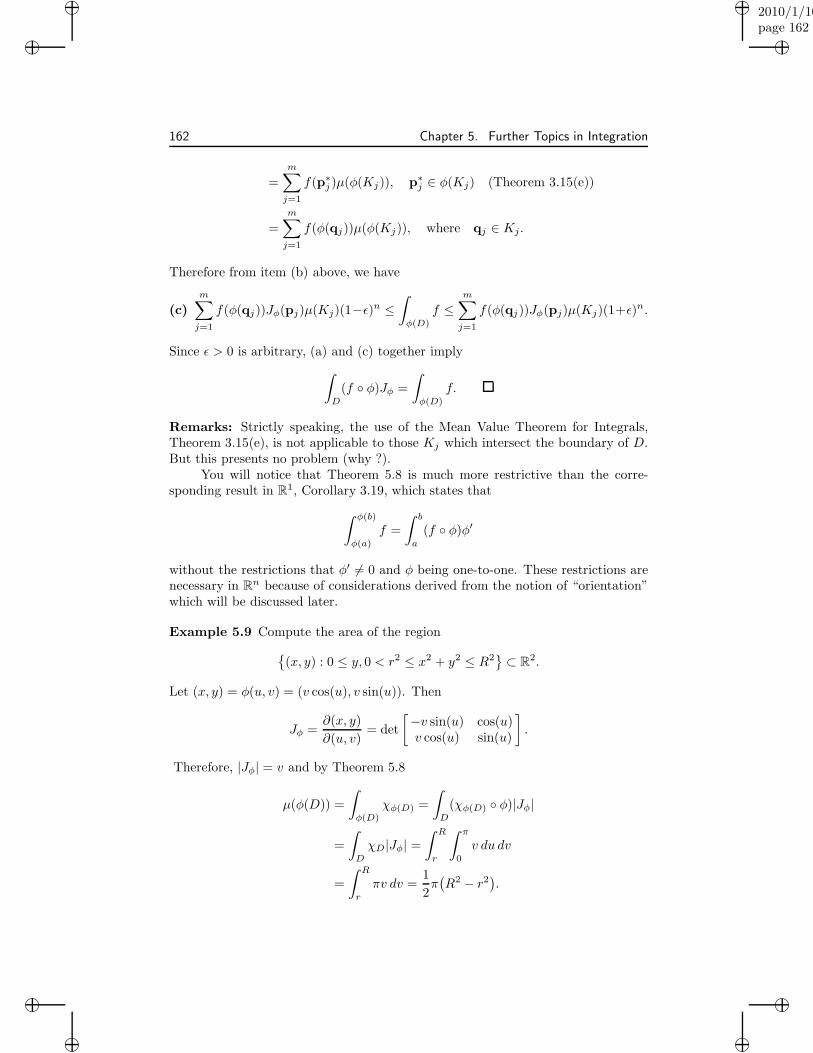
“muldowney”2010/1/10page 162
i
i
i
i
i
i
i
i
162 Chapter 5. Further Topics in Integration
=m∑
j=1
f(p∗j )µ(φ(Kj)), p∗
j ∈ φ(Kj) (Theorem 3.15(e))
=
m∑
j=1
f(φ(qj))µ(φ(Kj)), where qj ∈ Kj.
Therefore from item (b) above, we have
(c)
m∑
j=1
f(φ(qj))Jφ(pj)µ(Kj)(1−ǫ)n ≤∫
φ(D)
f ≤m∑
j=1
f(φ(qj))Jφ(pj)µ(Kj)(1+ǫ)n.
Since ǫ > 0 is arbitrary, (a) and (c) together imply
∫
D
(f ◦ φ)Jφ =
∫
φ(D)
f.
Remarks: Strictly speaking, the use of the Mean Value Theorem for Integrals,Theorem 3.15(e), is not applicable to those Kj which intersect the boundary of D.But this presents no problem (why ?).
You will notice that Theorem 5.8 is much more restrictive than the corre-sponding result in R1, Corollary 3.19, which states that
∫ φ(b)
φ(a)
f =
∫ b
a
(f ◦ φ)φ′
without the restrictions that φ′ 6= 0 and φ being one-to-one. These restrictions arenecessary in Rn because of considerations derived from the notion of “orientation”which will be discussed later.
Example 5.9 Compute the area of the region
{(x, y) : 0 ≤ y, 0 < r2 ≤ x2 + y2 ≤ R2
}⊂ R2.
Let (x, y) = φ(u, v) = (v cos(u), v sin(u)). Then
Jφ =∂(x, y)
∂(u, v)= det
[−v sin(u) cos(u)v cos(u) sin(u)
].
Therefore, |Jφ| = v and by Theorem 5.8
µ(φ(D)) =
∫
φ(D)
χφ(D) =
∫
D
(χφ(D) ◦ φ)|Jφ|
=
∫
D
χD|Jφ| =∫ R
r
∫ π
0
v du dv
=
∫ R
r
πv dv =1
2π(R2 − r2
).
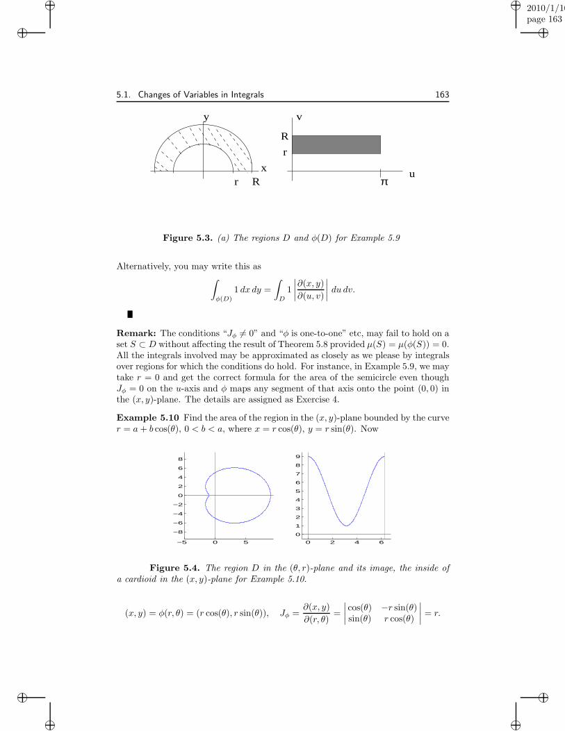
“muldowney”2010/1/10page 163
i
i
i
i
i
i
i
i
5.1. Changes of Variables in Integrals 163
π
r
R
Rru
v
x
y
Figure 5.3. (a) The regions D and φ(D) for Example 5.9
Alternatively, you may write this as∫
φ(D)
1 dx dy =
∫
D
1
∣∣∣∣∂(x, y)
∂(u, v)
∣∣∣∣ du dv.
Remark: The conditions “Jφ 6= 0” and “φ is one-to-one” etc, may fail to hold on aset S ⊂ D without affecting the result of Theorem 5.8 provided µ(S) = µ(φ(S)) = 0.All the integrals involved may be approximated as closely as we please by integralsover regions for which the conditions do hold. For instance, in Example 5.9, we maytake r = 0 and get the correct formula for the area of the semicircle even thoughJφ = 0 on the u-axis and φ maps any segment of that axis onto the point (0, 0) inthe (x, y)-plane. The details are assigned as Exercise 4.
Example 5.10 Find the area of the region in the (x, y)-plane bounded by the curver = a+ b cos(θ), 0 < b < a, where x = r cos(θ), y = r sin(θ). Now
−5 0 5
−8
−6
−4
−2
0
2
4
6
8
0 2 4 6
0
1
2
3
4
5
6
7
8
9
Figure 5.4. The region D in the (θ, r)-plane and its image, the inside ofa cardioid in the (x, y)-plane for Example 5.10.
(x, y) = φ(r, θ) = (r cos(θ), r sin(θ)), Jφ =∂(x, y)
∂(r, θ)=
∣∣∣∣cos(θ) −r sin(θ)sin(θ) r cos(θ)
∣∣∣∣ = r.
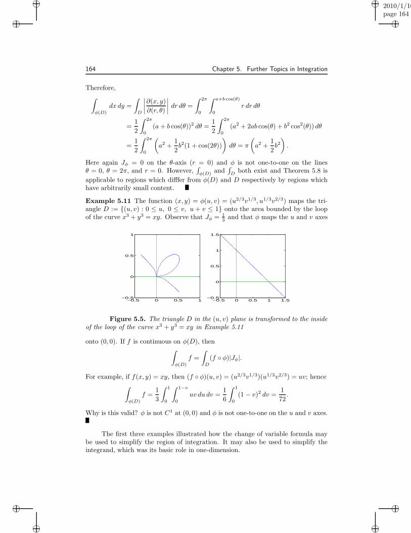
“muldowney”2010/1/10page 164
i
i
i
i
i
i
i
i
164 Chapter 5. Further Topics in Integration
Therefore,
∫
φ(D)
dx dy =
∫
D
∣∣∣∣∂(x, y)
∂(r, θ)
∣∣∣∣ dr dθ =
∫ 2π
0
∫ a+b cos(θ)
0
r dr dθ
=1
2
∫ 2π
0
(a+ b cos(θ))2 dθ =1
2
∫ 2π
0
(a2 + 2ab cos(θ) + b2 cos2(θ)) dθ
=1
2
∫ 2π
0
(a2 +
1
2b2(1 + cos(2θ))
)dθ = π
(a2 +
1
2b2).
Here again Jφ = 0 on the θ-axis (r = 0) and φ is not one-to-one on the linesθ = 0, θ = 2π, and r = 0. However,
∫φ(D) and
∫D both exist and Theorem 5.8 is
applicable to regions which difffer from φ(D) and D respectively by regions whichhave arbitrarily small content.
Example 5.11 The function (x, y) = φ(u, v) = (u2/3v1/3, u1/3v2/3) maps the tri-angle D := {(u, v) : 0 ≤ u, 0 ≤ v, u + v ≤ 1} onto the area bounded by the loopof the curve x3 + y3 = xy. Observe that Jφ = 1
3 and that φ maps the u and v axes
−0.5 0 0.5 1−0.5
0
0.5
1
−0.5 0 0.5 1 1.5−0.5
0
0.5
1
1.5
Figure 5.5. The triangle D in the (u, v) plane is transformed to the insideof the loop of the curve x3 + y3 = xy in Example 5.11
onto (0, 0). If f is continuous on φ(D), then∫
φ(D)
f =
∫
D
(f ◦ φ)|Jφ|.
For example, if f(x, y) = xy, then (f ◦ φ)(u, v) = (u2/3v1/3)(u1/3v2/3) = uv; hence
∫
φ(D)
f =1
3
∫ 1
0
∫ 1−v
0
uv du dv =1
6
∫ 1
0
(1 − v)2 dv =1
72.
Why is this valid? φ is not C1 at (0, 0) and φ is not one-to-one on the u and v axes.
The first three examples illustrated how the change of variable formula maybe used to simplify the region of integration. It may also be used to simplify theintegrand, which was its basic role in one-dimension.
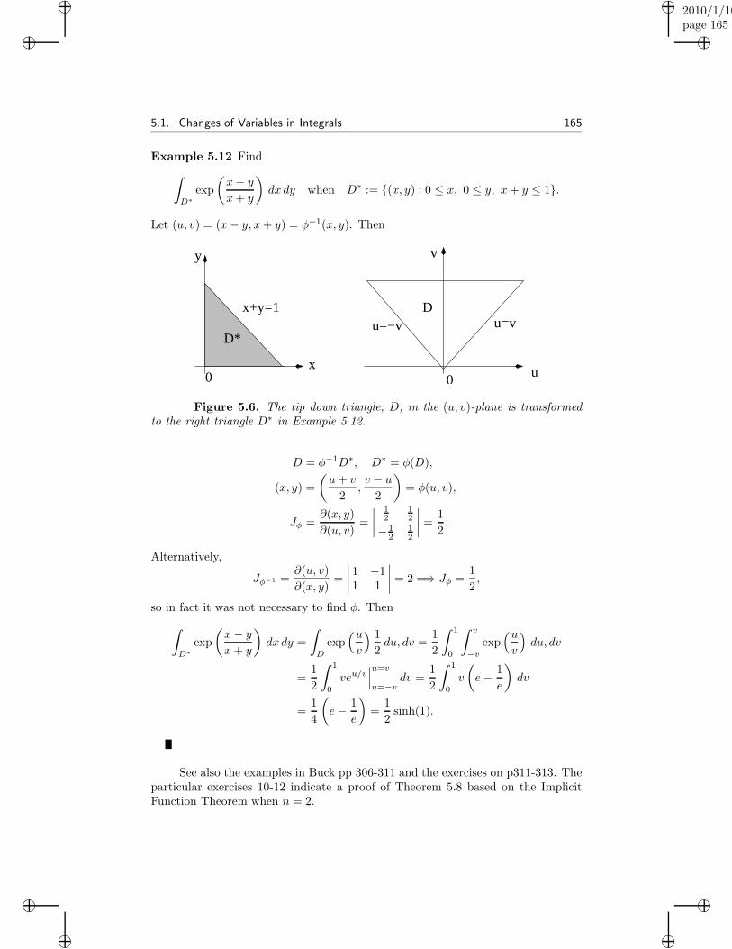
“muldowney”2010/1/10page 165
i
i
i
i
i
i
i
i
5.1. Changes of Variables in Integrals 165
Example 5.12 Find
∫
D∗
exp
(x− yx+ y
)dx dy when D∗ := {(x, y) : 0 ≤ x, 0 ≤ y, x+ y ≤ 1}.
Let (u, v) = (x− y, x+ y) = φ−1(x, y). Then
x+y=1
x0
D*
y
D
u
v
u=vu=−v
0
Figure 5.6. The tip down triangle, D, in the (u, v)-plane is transformedto the right triangle D∗ in Example 5.12.
D = φ−1D∗, D∗ = φ(D),
(x, y) =
(u+ v
2,v − u
2
)= φ(u, v),
Jφ =∂(x, y)
∂(u, v)=
∣∣∣∣12
12
− 12
12
∣∣∣∣ =1
2.
Alternatively,
Jφ−1 =∂(u, v)
∂(x, y)=
∣∣∣∣1 −11 1
∣∣∣∣ = 2 =⇒ Jφ =1
2,
so in fact it was not necessary to find φ. Then
∫
D∗
exp
(x− yx+ y
)dx dy =
∫
D
exp(uv
) 1
2du, dv =
1
2
∫ 1
0
∫ v
−vexp
(uv
)du, dv
=1
2
∫ 1
0
veu/v∣∣∣u=v
u=−vdv =
1
2
∫ 1
0
v
(e− 1
e
)dv
=1
4
(e− 1
e
)=
1
2sinh(1).
See also the examples in Buck pp 306-311 and the exercises on p311-313. Theparticular exercises 10-12 indicate a proof of Theorem 5.8 based on the ImplicitFunction Theorem when n = 2.
“muldowney”2010/1/10page 166
i
i
i
i
i
i
i
i
166 Chapter 5. Further Topics in Integration
Exercises
5.1. For f1(x, y) = x2
a2 + y2
b2 and f2(x, y) = x2 + y2, find
∫
D
f1 and
∫
D
f2 where D =
{(x, y) :
x2
a2+y2
b2≤ 1
}.
[Solution: πab/2, πab(a2 + b2)/4.]
5.2. Let f be a real valued continuous function on R2. Show that
∫ 1
0
[∫ x
0
f(x, y) dy
]dx = 2
∫ 1/2
0
[∫ 1−η
η
f(ξ + η, ξ − η) dξ]dη.
5.3. Do the following:
(i) Show that the ball S = {(x, y, z) : x2 + y2 + z2 ≤ a2} has contentM = 4πa3/3 in R3. [Hint: Let x = r sin(φ) cos(θ), y = r sin(φ) cos(θ),and z = r cos(φ), for 0 ≤ r ≤ a, 0 ≤ θ ≤ 2π, 0 ≤ φ ≤ π.]
(ii) Let S be as in part (i) and show
Iz :=
∫
S
(x2 + y2) dx dy dz =2Ma2
5.
[Iz is the moment of inertia of a uniform spherical mass distribution(total mass = M) about a diameter. The quantity
√2a2/5 is called the
radius of gyration about a diameter.]
5.4. (The case of the vanishing Jacobian) Suppose φ : Rn 7→ Rn is of class C1 onan open set G ⊂ Rn and that Jφ 6= 0 and φ is one-to-one except on a set Kwith content zero. Suppose D ⊂ G is compact and has content, and f is areal valued continuous function on φ(D). Show that φ(D) has content and
∫
φ(D)
f =
∫
D
(f ◦ φ)|Jφ|.
[Hint: For a given ǫ, enclose K in the union U of a finite number of n-cubessuch that µ(U) < ǫ. Apply Theorem 5.8 to D\U .]
5.5. Show that∫
K
[(x− y)2 + 2(x+ y) + 1
]−1/2dx dy = 2 log(2)− 1
2
where K is the triangle bounded by x = 0, y = 2, and x = y. [Hint:x = u(1 + v), y = v(1 + u).]
5.6. Evaluate∫D1f and
∫D2f where
f(x, y) =1
(1 + x2 + y2)2
“muldowney”2010/1/10page 167
i
i
i
i
i
i
i
i
5.1. Changes of Variables in Integrals 167
and (i) D1 is the region bounded by one loop of the lemiscate
(x2 + y2)2 − (x2 − y2) = 0;
and (ii) D2 is the triangle with vertices (0, 0), (2, 0), (1,√
3). [Solution: π4 − 1
2
and√
32 arctan(1/2).]
5.7. Show that
∫
K
|xyz| dx dy dz =a2b2c2
6where K :=
{(x, y, x) :
x2
a2+y2
b2+z2
c2≤ 1
}.
5.8. Let ψ(x, y) = Ax2 + 2Hxy +By2 + 2Gx+ 2Fy + C.
(i) Show
∫
K
ψ =1
4πab(Aa2+Bb2+4C) where K :=
{(x, y, ) :
x2
a2+y2
b2≤ 1
}.
Save yourself some work by using symmetry to show
∫
K
xy dx dy =
∫
K
xdx dy =
∫
K
y dx dy = 0.
(ii) Show ∫H ψ = 1
4πab(Aa2 +Bb2 + 4ψ(x0, y0)) where
H :={
(x, y, ) : (x−x0)2
a2 + (y−y0)2b2 ≤ 1
}.
(iii) Show
∫S(2x2 + y2 + 3x− 2y + 4) dx dy = 57π
2 where
S is inside x2 + 4y2 − 2x+ 8y + 1 = 0.
(iv) If the plane ℓx+my + nz = p intersects the elliptic paraboloid
x2
a2+y2
b2= 2
z
c,
show that the volume of the solid bounded by these two surfaces is
πab
4c3n4(a2ℓ2 + b2m2 + 2pcn)2.
5.9. Find∫
D
log(x2 + y2) dx dy where D := {(x, y) : b2 ≤ (x2 + y2) ≤ a2}
and show that the limit as b→ 0 of this expression is 2πa2(log(a)− 12 ).
“muldowney”2010/1/10page 168
i
i
i
i
i
i
i
i
168 Chapter 5. Further Topics in Integration
5.10. Show that∫Dx3y2 dx dy = 248 2
5 , where D is the region bounded by the linesy = ±3(x − 2), y = ±3(x − 4). [Hint: Move the origin to the center of theregion and use symmetry as much as you can.]
5.11. Show that the area of the region in the first quadrant bounded by
y3 = a1x2, y3 = a2x
2, a1 > a2 > 0, and
xy2 = b31, xy2 = b32, b1 > b2 ≥ 0, is
Area =7
5
(b15/71 − b15/72
)(a−1/72 − a−1/7
1
).
5.12. Show that the area of the region bounded by the loop of the curve x3 + y3 =3axy is 3a2/2.
5.13. The transformation x = umφ(v), y = unψ(v) maps the rectangle [u1, u2] ×[v1, v2] into a region in the (x, y)-plane. The area of this region is
∣∣∣(um+n1 − um+n
2 )∫ v2v1
mφψ′−nψφ′
m+n
∣∣∣ , if m 6= −n and
|m(φ(v1)ψ(v1)− φ(v2)φ(v2)) log(u1/u2)|, if m = −n.
What conditions must φ and ψ satisfy if this statement is correct? Prove thestatement under your conditions.
5.14. Find∫Dxyz dx dy dz where D is the region in the first octant bounded by
the cylinder x2 + y2 = 16 and the plane z = 3, that is,
D ={(x, y, z) : 0 ≤ x, 0 ≤ y, 0 ≤ z ≤ 3, x2 + y2 ≤ 16
}.
5.15. Let G be the region in the first quadrant which is bounded by the curvesxy = 1, xy = 3, x2 − y2 = 1, x2 − y2 = 4. Find
∫G F where F (x, y) = xy.
5.16. Show ∫
D
φ =1
3pq(ap2 + bq2) + 2pqφ(x0, y0)
where D is the region bounded by the four straight lines
x− x0
p± y − y0
q= ±1 (p.q > 0)
and φ(x, y) = ax2 + 2hxy + by2 + 2gx+ 2fy + c.
5.17. Show the following:
(i) If X = x+ y+ z + u, XY = y+ z + u, XY Z = z + u, XY ZU = u. showthat
∂(x, y, z, u)
∂(X,Y, Z, U)= X3Y 2Z.
(ii) Show that
∫ 1
0
∫ 1−u
0
∫ 1−z−u
0
∫ 1−y−z−u
0
(x+ y + z + u)nxyzu dx dy dz du =
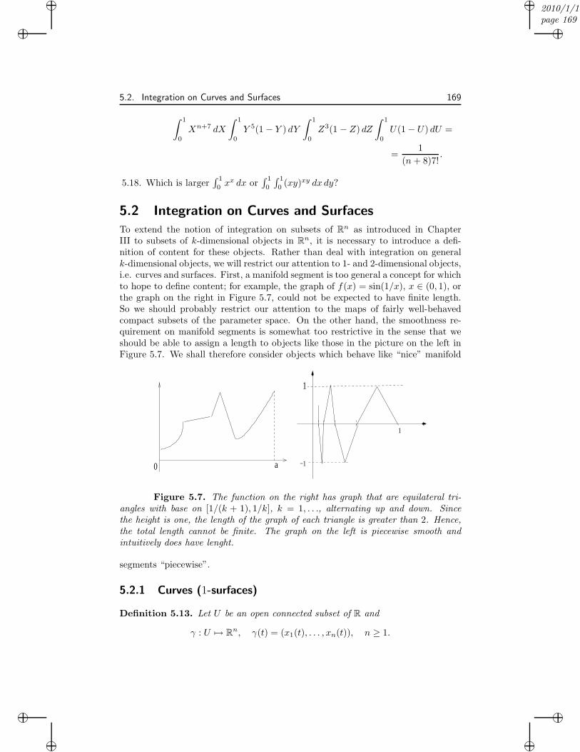
“muldowney”2010/1/10page 169
i
i
i
i
i
i
i
i
5.2. Integration on Curves and Surfaces 169
∫ 1
0
Xn+7 dX
∫ 1
0
Y 5(1− Y ) dY
∫ 1
0
Z3(1 − Z) dZ
∫ 1
0
U(1− U) dU =
=1
(n+ 8)7!.
5.18. Which is larger∫ 1
0xx dx or
∫ 1
0
∫ 1
0(xy)xy dx dy?
5.2 Integration on Curves and Surfaces
To extend the notion of integration on subsets of Rn as introduced in ChapterIII to subsets of k-dimensional objects in Rn, it is necessary to introduce a defi-nition of content for these objects. Rather than deal with integration on generalk-dimensional objects, we will restrict our attention to 1- and 2-dimensional objects,i.e. curves and surfaces. First, a manifold segment is too general a concept for whichto hope to define content; for example, the graph of f(x) = sin(1/x), x ∈ (0, 1), orthe graph on the right in Figure 5.7, could not be expected to have finite length.So we should probably restrict our attention to the maps of fairly well-behavedcompact subsets of the parameter space. On the other hand, the smoothness re-quirement on manifold segments is somewhat too restrictive in the sense that weshould be able to assign a length to objects like those in the picture on the left inFigure 5.7. We shall therefore consider objects which behave like “nice” manifold
1
−1
1
0 a
Figure 5.7. The function on the right has graph that are equilateral tri-angles with base on [1/(k + 1), 1/k], k = 1, . . ., alternating up and down. Sincethe height is one, the length of the graph of each triangle is greater than 2. Hence,the total length cannot be finite. The graph on the left is piecewise smooth andintuitively does have lenght.
segments “piecewise”.
5.2.1 Curves (1-surfaces)
Definition 5.13. Let U be an open connected subset of R and
γ : U 7→ Rn, γ(t) = (x1(t), . . . , xn(t)), n ≥ 1.
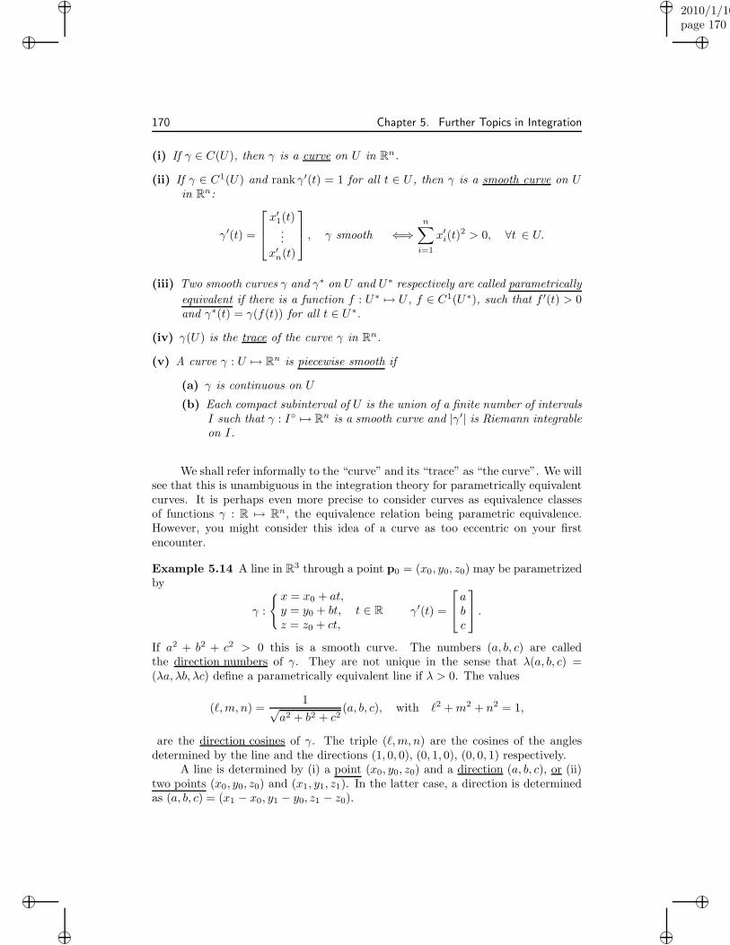
“muldowney”2010/1/10page 170
i
i
i
i
i
i
i
i
170 Chapter 5. Further Topics in Integration
(i) If γ ∈ C(U), then γ is a curve on U in Rn.
(ii) If γ ∈ C1(U) and rank γ′(t) = 1 for all t ∈ U , then γ is a smooth curve on Uin Rn:
γ′(t) =
x′1(t)
...x′n(t)
, γ smooth ⇐⇒
n∑
i=1
x′i(t)2 > 0, ∀t ∈ U.
(iii) Two smooth curves γ and γ∗ on U and U∗ respectively are called parametrically
equivalent if there is a function f : U∗ 7→ U , f ∈ C1(U∗), such that f ′(t) > 0and γ∗(t) = γ(f(t)) for all t ∈ U∗.
(iv) γ(U) is the trace of the curve γ in Rn.
(v) A curve γ : U 7→ Rn is piecewise smooth if
(a) γ is continuous on U
(b) Each compact subinterval of U is the union of a finite number of intervalsI such that γ : I◦ 7→ Rn is a smooth curve and |γ′| is Riemann integrableon I.
We shall refer informally to the “curve” and its “trace” as “the curve”. We willsee that this is unambiguous in the integration theory for parametrically equivalentcurves. It is perhaps even more precise to consider curves as equivalence classesof functions γ : R 7→ Rn, the equivalence relation being parametric equivalence.However, you might consider this idea of a curve as too eccentric on your firstencounter.
Example 5.14 A line in R3 through a point p0 = (x0, y0, z0) may be parametrizedby
γ :
{x = x0 + at,y = y0 + bt, t ∈ R
z = z0 + ct,γ′(t) =
abc
.
If a2 + b2 + c2 > 0 this is a smooth curve. The numbers (a, b, c) are calledthe direction numbers of γ. They are not unique in the sense that λ(a, b, c) =(λa, λb, λc) define a parametrically equivalent line if λ > 0. The values
(ℓ,m, n) =1√
a2 + b2 + c2(a, b, c), with ℓ2 +m2 + n2 = 1,
are the direction cosines of γ. The triple (ℓ,m, n) are the cosines of the anglesdetermined by the line and the directions (1, 0, 0), (0, 1, 0), (0, 0, 1) respectively.
A line is determined by (i) a point (x0, y0, z0) and a direction (a, b, c), or (ii)two points (x0, y0, z0) and (x1, y1, z1). In the latter case, a direction is determinedas (a, b, c) = (x1 − x0, y1 − y0, z1 − z0).
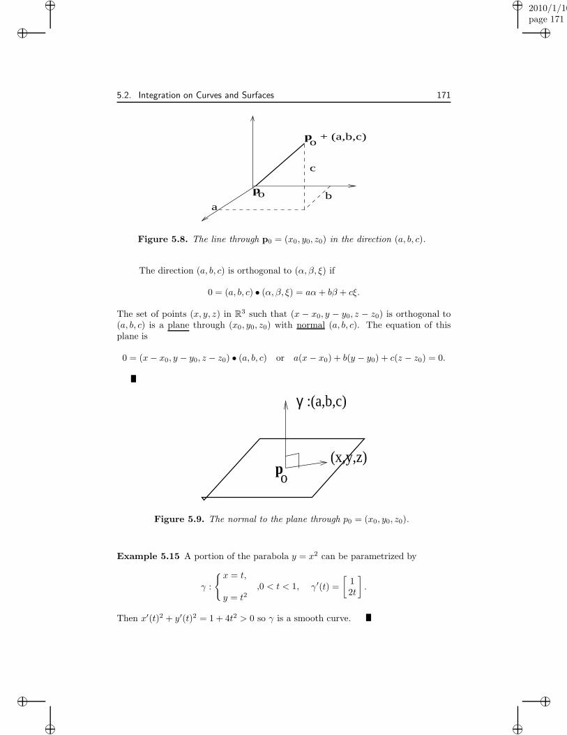
“muldowney”2010/1/10page 171
i
i
i
i
i
i
i
i
5.2. Integration on Curves and Surfaces 171
ab
c
+ (a,b,c)
po
po
Figure 5.8. The line through p0 = (x0, y0, z0) in the direction (a, b, c).
The direction (a, b, c) is orthogonal to (α, β, ξ) if
0 = (a, b, c) • (α, β, ξ) = aα+ bβ + cξ.
The set of points (x, y, z) in R3 such that (x − x0, y − y0, z − z0) is orthogonal to(a, b, c) is a plane through (x0, y0, z0) with normal (a, b, c). The equation of thisplane is
0 = (x− x0, y − y0, z − z0) • (a, b, c) or a(x− x0) + b(y − y0) + c(z − z0) = 0.
(x,y,z)
:(a,b,c)γ
po
Figure 5.9. The normal to the plane through p0 = (x0, y0, z0).
Example 5.15 A portion of the parabola y = x2 can be parametrized by
γ :
{x = t,,0 < t < 1,
y = t2γ′(t) =
[12t
].
Then x′(t)2 + y′(t)2 = 1 + 4t2 > 0 so γ is a smooth curve.
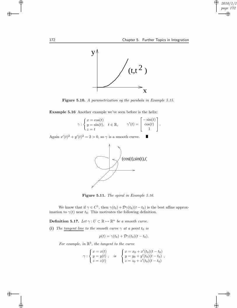
“muldowney”2010/1/10page 172
i
i
i
i
i
i
i
i
172 Chapter 5. Further Topics in Integration
x
y
(t,t 2 )
Figure 5.10. A parametrization og the parabola in Example 5.15.
Example 5.16 Another example we’ve seen before is the helix:
γ :
{x = cos(t)y = sin(t), t ∈ R,z = t
γ′(t) =
− sin(t)cos(t)
1
.
Again x′(t)2 + y′(t)2 = 2 > 0, so γ is a smooth curve.
(cos(t),sin(t),t)
Figure 5.11. The spiral in Example 5.16.
We know that if γ ∈ C1, then γ(t0) +Dγ(t0)(t− t0) is the best affine approx-imation to γ(t) near t0. This motivates the following definition.
Definition 5.17. Let γ : U ⊂ R 7→ Rn be a smooth curve.
(i) The tangent line to the smooth curve γ at a point t0 is
p(t) = γ(t0) +Dγ(t0)(t− t0).
For example, in R3, the tangent to the curve
γ :
x = x(t)y = y(t)z = z(t)
, is
x = x0 + x′(t0)(t− t0)y = y0 + y′(t0)(t− t0)z = z0 + z′(t0)(t− t0)
,
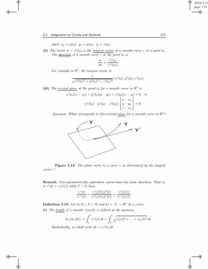
“muldowney”2010/1/10page 173
i
i
i
i
i
i
i
i
5.2. Integration on Curves and Surfaces 173
where x0 = x(t0), y0 = y(t0), z0 = z(t0).
(ii) The vector v = γ′(t0) is the tangent vector of a smooth curve γ at a point t0.The direction of a smooth curve γ at the point t0 is
v
|v| =γ′(t0)
|γ′(t0)|.
For example in R3, the tangent vector is
1√x′(t0)2 + y′(t0)2 + z′(t0)2
(x′(t0), y′(t0), z
′(t0)) .
(iii) The normal plane at the point t0 for a smooth curve in R3 is
x′(t0)(x− x0) + y′(t0)(y − y0) + z′(t0)(z − z0) = 0 or
[x′(t0) y′(t0) z′(t0) ]
x− x0
y − y0z − z0
= 0.
Question: What corresponds to this normal plane for a smooth curve in R2?
γ’γγ
Figure 5.12. The plane norm to a curve γ as determined by the tangentvector γ′.
Remark: Two parametrically equivalent curves have the same direction. That is,if γ∗(t) = γ(f(t)) with f ′ > 0, then
γ∗(t)
|γ∗(t)| =γ′(f(t))f ′(t)
|γ′(f(t))f ′(t)| =γ′(f(t))
|γ′(f(t))| .
Definition 5.18. Let [a, b] ⊂ U ⊂ R and let γ : U 7→ Rn be a curve.
(i) The length of a smooth γ([a, b]) is defined as the quantity
ℓ(γ([a, b])) :=
∫ b
a
|γ′(t)| dt =
∫ b
a
√x′1(t)
2 + . . .+ x′n(t)2 dt.
Symbolically, we shall write dℓ = |γ′(t)| dt.
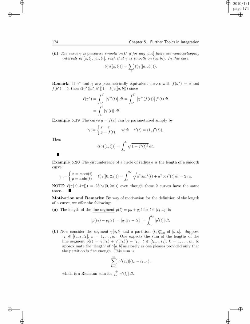
“muldowney”2010/1/10page 174
i
i
i
i
i
i
i
i
174 Chapter 5. Further Topics in Integration
(ii) The curve γ is piecewise smooth on U if for any [a, b] there are nonoverlappingintervals of [a, b], [ai, bi], such that γ is smooth on (ai, bi). In this case.
ℓ(γ([a, b])) =∑
i
ℓ(γ([ai, bi])).
Remark: If γ∗ and γ are parametrically equivalent curves with f(a∗) = a andf(b∗) = b, then ℓ(γ∗([a∗, b∗])) = ℓ(γ([a, b])) since
ℓ(γ∗) =
∫ b∗
a∗
∣∣γ∗′(t)∣∣ dt =
∫ b∗
a∗
∣∣γ∗′(f(t))∣∣ f ′(t) dt
=
∫ b
a
|γ′(t)| dt.
Example 5.19 The curve y = f(x) can be parametrized simply by
γ :=
{x = ty = f(t),
with γ′(t) = (1, f ′(t)).
Then
ℓ(γ([a, b])) =
∫ b
a
√1 + f ′(t)2 dt.
Example 5.20 The circumference of a circle of radius a is the length of a smoothcurve:
γ :=
{x = a cos(t)y = a sin(t)
ℓ(γ([0, 2π])) =
∫ 2π
0
√a2 sin2(t) + a2 cos2(t) dt = 2πa.
NOTE: ℓ(γ([0, 4π])) = 2ℓ(γ([0, 2π])) even though these 2 curves have the sametrace.
Motivation and Remarks: By way of motivation for the definition of the lengthof a curve, we offer the following:
(a) The length of the line segment p(t) = p0 + q0t for t ∈ [t1, t2] is
|p(t2)− p(t1)| = |q0(t2 − t1)| =∫ t2
t1
|p′(t)| dt.
(b) Now consider the segment γ[a, b] and a partition (tk)mk=0 of [a, b]. Suppose
τk ∈ [tk−1, tk], k = 1, . . . ,m. One expects the sum of the lengths of theline segment p(t) = γ(τk) + γ′(τk)(t − τk), t ∈ [tk−1, tk], k = 1, . . . ,m, toapproximate the ‘length’ of γ[a, b] as closely as one pleases provided only thatthe partition is fine enough. This sum is
m∑
k=1
|γ′(τk)|(tk − tk−1),
which is a Riemann sum for∫ ba|γ′(t)| dt.
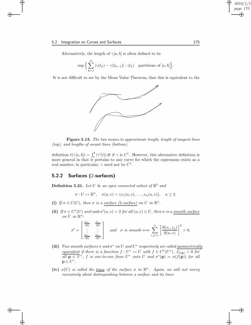
“muldowney”2010/1/10page 175
i
i
i
i
i
i
i
i
5.2. Integration on Curves and Surfaces 175
Alternatively, the length of γ[a, b] is often defined to be
sup{ m∑
k=1
|γ(tk)− γ(tk−1)| : (tk) partitions of [a, b]}.
It is not difficult to see by the Mean Value Theorem, that this is equivalent to the
Figure 5.13. The two means to approximate length, length of tangent lines(top), and lengths of secant lines (bottom).
definition ℓ(γ[a, b]) =∫ ba |γ′(t)| dt if γ is C1. However, this alternative definition is
more general in that it pertains to any curve for which the supremum exists as areal number; in particular, γ need not be C1.
5.2.2 Surfaces (2-surfaces)
Definition 5.21. Let U be an open connected subset of R2 and
σ : U 7→ Rn, σ(u, v) = (x1(u, v), . . . , xn(u, v)), n ≥ 2.
(i) If σ ∈ C(U), then σ is a surface (2-surface) on U in Rn.
(ii) If σ ∈ C1(U) and rankσ′(u, v) = 2 for all (u, v) ∈ U , then σ is a smooth surfaceon U in Rn:
σ′ =
∂x1
∂u∂x1
∂v...
...∂xn
∂u∂xn
∂v
and σ is smooth⇐⇒
n∑
i,j=1
[∂(xi, xj)
∂(u, v)
]2> 0.
(iii) Two smooth surfaces σ and σ∗ on U and U∗ respectively are called parametrically
equivalent if there is a function f : U∗ 7→ U with f ∈ C1(U∗), Jf(p) > 0 forall p ∈ U∗, f is one-to-one from U∗ onto U and σ∗(p) = σ(f(p)) for allp ∈ U∗.
(iv) σ(U) is called the trace of the surface σ in Rn. Again, we will not worryexcessively about distinguishing between a surface and its trace.
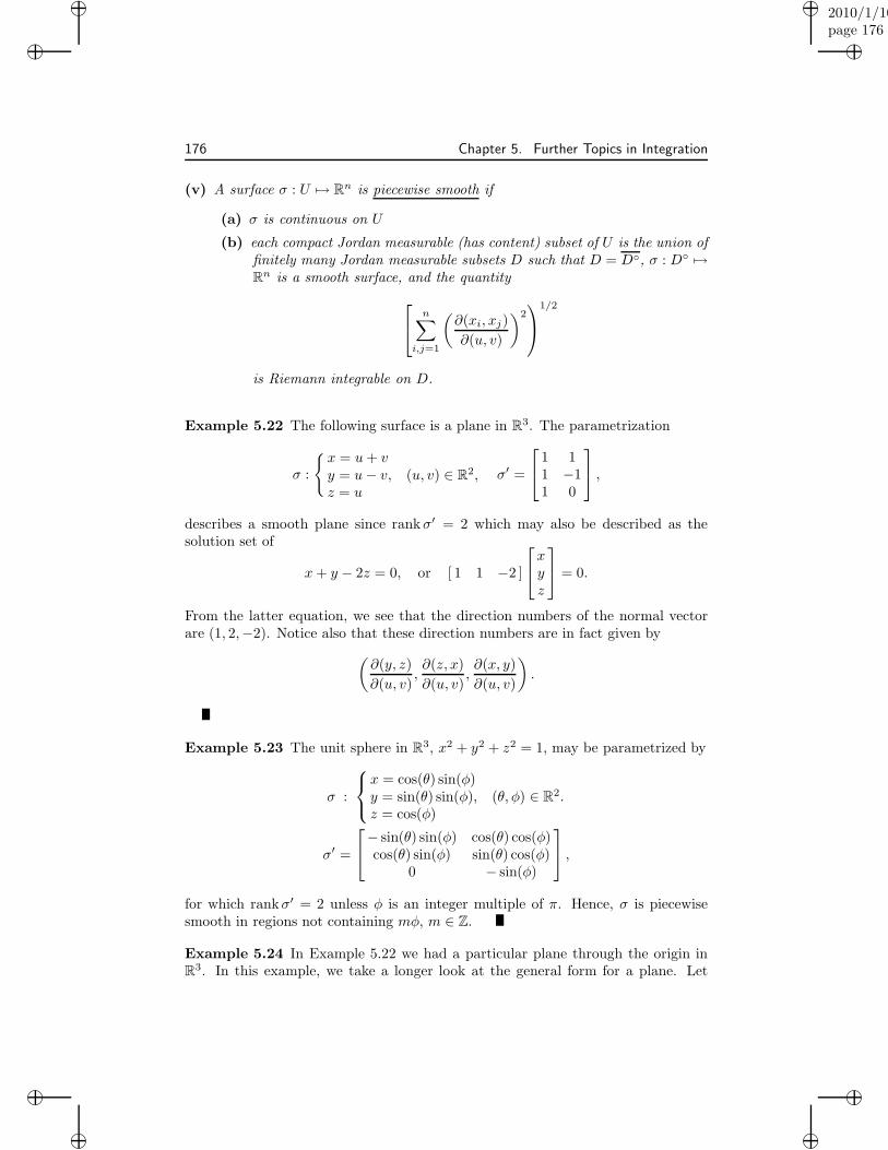
“muldowney”2010/1/10page 176
i
i
i
i
i
i
i
i
176 Chapter 5. Further Topics in Integration
(v) A surface σ : U 7→ Rn is piecewise smooth if
(a) σ is continuous on U
(b) each compact Jordan measurable (has content) subset of U is the union offinitely many Jordan measurable subsets D such that D = D◦, σ : D◦ 7→Rn is a smooth surface, and the quantity
n∑
i,j=1
(∂(xi, xj)
∂(u, v)
)2
1/2
is Riemann integrable on D.
Example 5.22 The following surface is a plane in R3. The parametrization
σ :
{x = u+ vy = u− v, (u, v) ∈ R2,z = u
σ′ =
1 11 −11 0
,
describes a smooth plane since rankσ′ = 2 which may also be described as thesolution set of
x+ y − 2z = 0, or [ 1 1 −2 ]
xyz
= 0.
From the latter equation, we see that the direction numbers of the normal vectorare (1, 2,−2). Notice also that these direction numbers are in fact given by
(∂(y, z)
∂(u, v),∂(z, x)
∂(u, v),∂(x, y)
∂(u, v)
).
Example 5.23 The unit sphere in R3, x2 + y2 + z2 = 1, may be parametrized by
σ :
x = cos(θ) sin(φ)y = sin(θ) sin(φ), (θ, φ) ∈ R2.z = cos(φ)
σ′ =
− sin(θ) sin(φ) cos(θ) cos(φ)cos(θ) sin(φ) sin(θ) cos(φ)
0 − sin(φ)
,
for which rankσ′ = 2 unless φ is an integer multiple of π. Hence, σ is piecewisesmooth in regions not containing mφ, m ∈ Z.
Example 5.24 In Example 5.22 we had a particular plane through the origin inR3. In this example, we take a longer look at the general form for a plane. Let
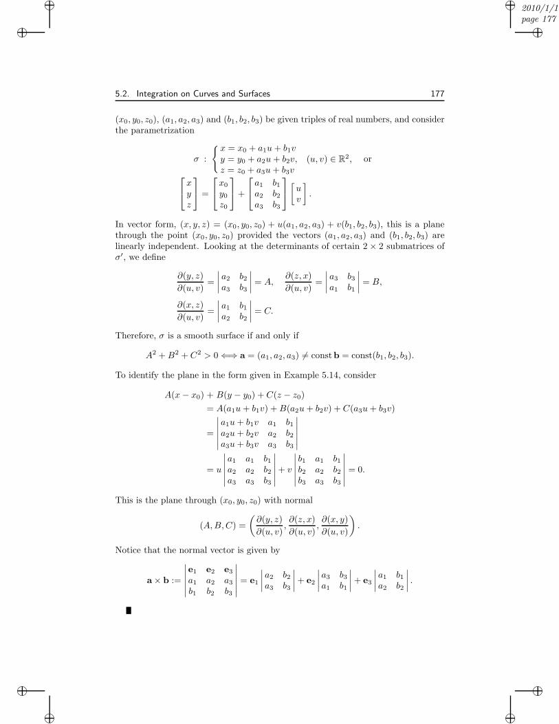
“muldowney”2010/1/10page 177
i
i
i
i
i
i
i
i
5.2. Integration on Curves and Surfaces 177
(x0, y0, z0), (a1, a2, a3) and (b1, b2, b3) be given triples of real numbers, and considerthe parametrization
σ :
{x = x0 + a1u+ b1vy = y0 + a2u+ b2v, (u, v) ∈ R2,z = z0 + a3u+ b3v
or
xyz
=
x0
y0z0
+
a1 b1a2 b2a3 b3
[uv
].
In vector form, (x, y, z) = (x0, y0, z0) + u(a1, a2, a3) + v(b1, b2, b3), this is a planethrough the point (x0, y0, z0) provided the vectors (a1, a2, a3) and (b1, b2, b3) arelinearly independent. Looking at the determinants of certain 2 × 2 submatrices ofσ′, we define
∂(y, z)
∂(u, v)=
∣∣∣∣a2 b2a3 b3
∣∣∣∣ = A,∂(z, x)
∂(u, v)=
∣∣∣∣a3 b3a1 b1
∣∣∣∣ = B,
∂(x, z)
∂(u, v)=
∣∣∣∣a1 b1a2 b2
∣∣∣∣ = C.
Therefore, σ is a smooth surface if and only if
A2 +B2 + C2 > 0⇐⇒ a = (a1, a2, a3) 6= constb = const(b1, b2, b3).
To identify the plane in the form given in Example 5.14, consider
A(x − x0) + B(y − y0) + C(z − z0)= A(a1u+ b1v) +B(a2u+ b2v) + C(a3u+ b3v)
=
∣∣∣∣∣∣
a1u+ b1v a1 b1a2u+ b2v a2 b2a3u+ b3v a3 b3
∣∣∣∣∣∣
= u
∣∣∣∣∣∣
a1 a1 b1a2 a2 b2a3 a3 b3
∣∣∣∣∣∣+ v
∣∣∣∣∣∣
b1 a1 b1b2 a2 b2b3 a3 b3
∣∣∣∣∣∣= 0.
This is the plane through (x0, y0, z0) with normal
(A,B,C) =
(∂(y, z)
∂(u, v),∂(z, x)
∂(u, v),∂(x, y)
∂(u, v)
).
Notice that the normal vector is given by
a× b :=
∣∣∣∣∣∣
e1 e2 e3
a1 a2 a3
b1 b2 b3
∣∣∣∣∣∣= e1
∣∣∣∣a2 b2a3 b3
∣∣∣∣+ e2
∣∣∣∣a3 b3a1 b1
∣∣∣∣+ e3
∣∣∣∣a1 b1a2 b2
∣∣∣∣ .
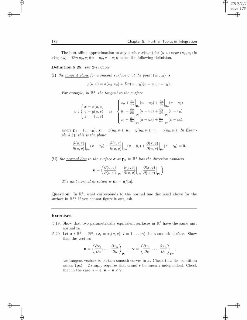
“muldowney”2010/1/10page 178
i
i
i
i
i
i
i
i
178 Chapter 5. Further Topics in Integration
The best affine approximation to any surface σ(u, v) for (u, v) near (u0, v0) isσ(u0, v0) +Dσ(u0, v0)(u − u0, v − v0); hence the following definition.
Definition 5.25. For 2-surfaces
(i) the tangent plane for a smooth surface σ at the point (u0, v0) is
p(u, v) = σ(u0, v0) +Dσ(u0, v0)(u − u0, v − v0).
For example, in R3, the tangent to the surface
σ :
x = x(u, v)y = y(u, v)z = z(u, v)
is
x0 + ∂x∂u
∣∣∣p0
(u− u0) + ∂x∂v
∣∣∣p0
(v − v0)
y0 + ∂y∂u
∣∣∣p0
(u− u0) + ∂y∂v
∣∣∣p0
(v − v0)
z0 + ∂z∂u
∣∣∣p0
(u− u0) + ∂z∂v
∣∣∣p0
(v − v0),
where p0 = (u0, v0), x0 = x(u0, v0), y0 = y(u0, v0), z0 = z(u0, v0). In Exam-ple 5.24, this is the plane
∂(y, z)
∂(u, v)
∣∣∣p0
(x− x0) +∂(z, x)
∂(u, v)
∣∣∣p0
(y − y0) +∂(x, y)
∂(u, v)
∣∣∣p0
(z − z0) = 0.
(ii) the normal line to the surface σ at p0 in R3 has the direction numbers
n =
(∂(u, v)
∂(u, v)
∣∣∣p0
,∂(z, x)
∂(u, v)
∣∣∣p0
,∂(x, y)
∂(u, v)
∣∣∣p0
).
The unit normal direction is n1 = n/|n|.
Question: In R4, what corresponds to the normal line discussed above for thesurface in R3? If you cannot figure it out, ask.
Exercises
5.19. Show that two parametrically equivalent surfaces in R3 have the same unitnormal n1.
5.20. Let σ : R2 7→ Rn, (xi = xi(u, v), i = 1, . . . , n), be a smooth surface. Showthat the vectors
u =
(∂x1
∂u, . . . ,
∂xn∂u
)
p0
, v =
(∂x1
∂v, . . . ,
∂xn∂v
)
p0
,
are tangent vectors to certain smooth curves in σ. Check that the conditionrankσ′(p0) = 2 simply requires that u and v be linearly independent. Checkthat in the case n = 3, n = u× v.
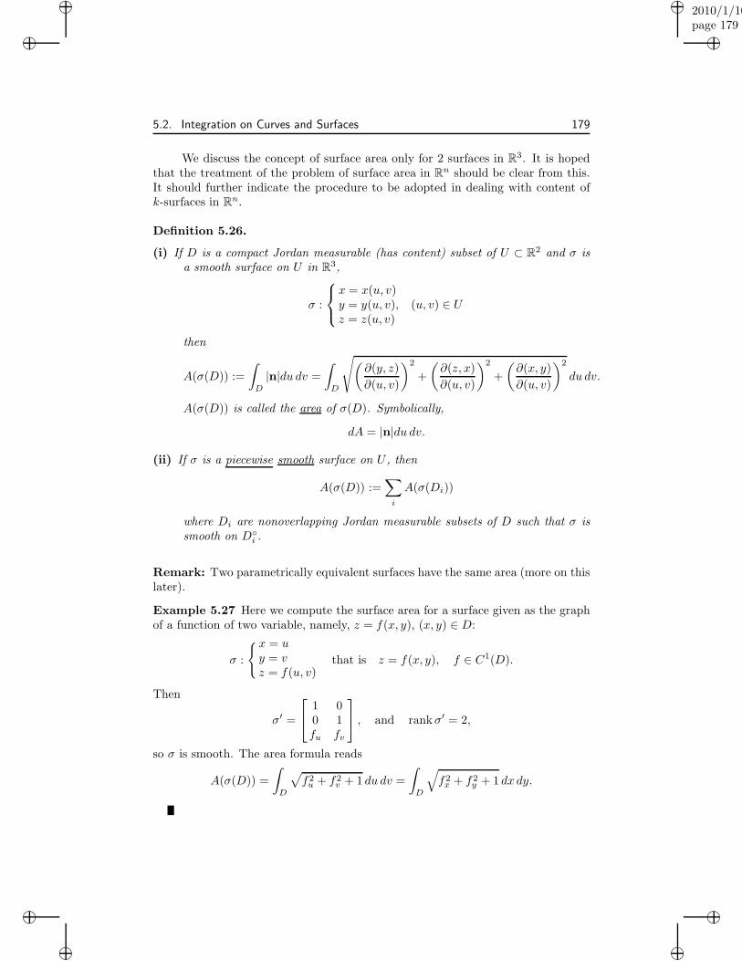
“muldowney”2010/1/10page 179
i
i
i
i
i
i
i
i
5.2. Integration on Curves and Surfaces 179
We discuss the concept of surface area only for 2 surfaces in R3. It is hopedthat the treatment of the problem of surface area in Rn should be clear from this.It should further indicate the procedure to be adopted in dealing with content ofk-surfaces in Rn.
Definition 5.26.
(i) If D is a compact Jordan measurable (has content) subset of U ⊂ R2 and σ isa smooth surface on U in R3,
σ :
x = x(u, v)y = y(u, v), (u, v) ∈ Uz = z(u, v)
then
A(σ(D)) :=
∫
D
|n|du dv =
∫
D
√(∂(y, z)
∂(u, v)
)2
+
(∂(z, x)
∂(u, v)
)2
+
(∂(x, y)
∂(u, v)
)2
du dv.
A(σ(D)) is called the area of σ(D). Symbolically,
dA = |n|du dv.
(ii) If σ is a piecewise smooth surface on U , then
A(σ(D)) :=∑
i
A(σ(Di))
where Di are nonoverlapping Jordan measurable subsets of D such that σ issmooth on D◦
i .
Remark: Two parametrically equivalent surfaces have the same area (more on thislater).
Example 5.27 Here we compute the surface area for a surface given as the graphof a function of two variable, namely, z = f(x, y), (x, y) ∈ D:
σ :
{x = uy = vz = f(u, v)
that is z = f(x, y), f ∈ C1(D).
Then
σ′ =
1 00 1fu fv
, and rankσ′ = 2,
so σ is smooth. The area formula reads
A(σ(D)) =
∫
D
√f2u + f2
v + 1 du dv =
∫
D
√f2x + f2
y + 1 dx dy.
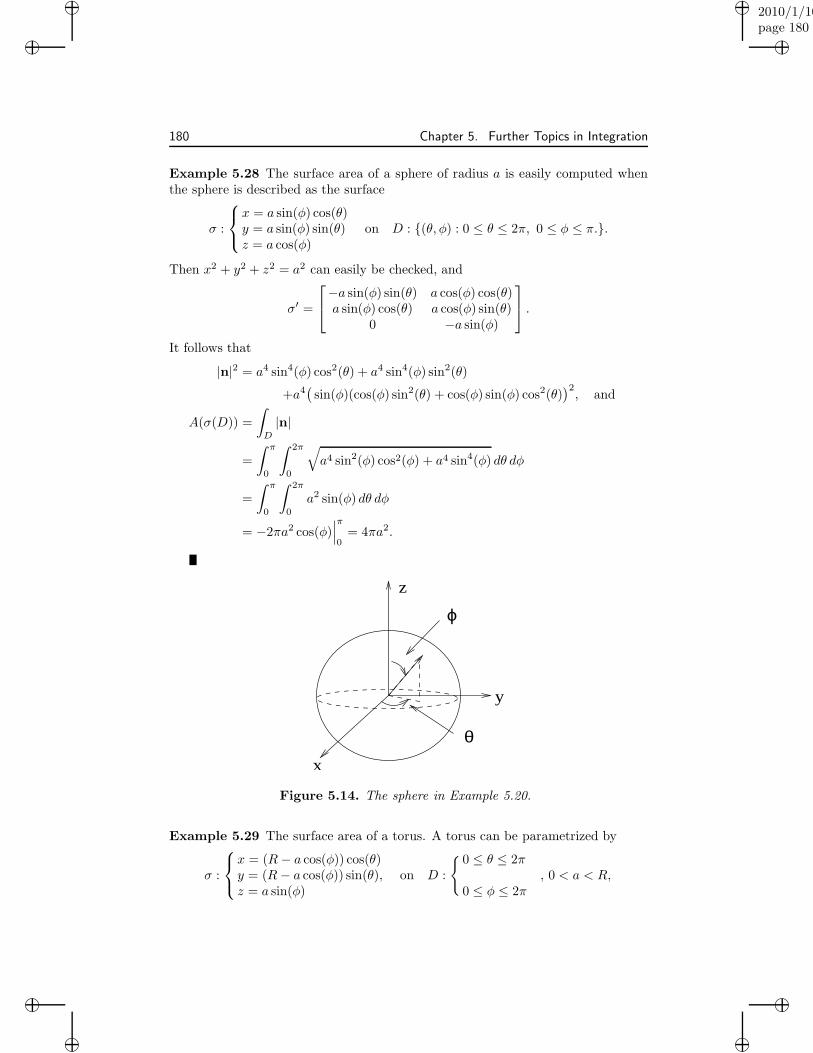
“muldowney”2010/1/10page 180
i
i
i
i
i
i
i
i
180 Chapter 5. Further Topics in Integration
Example 5.28 The surface area of a sphere of radius a is easily computed whenthe sphere is described as the surface
σ :
x = a sin(φ) cos(θ)y = a sin(φ) sin(θ)z = a cos(φ)
on D : {(θ, φ) : 0 ≤ θ ≤ 2π, 0 ≤ φ ≤ π.}.
Then x2 + y2 + z2 = a2 can easily be checked, and
σ′ =
−a sin(φ) sin(θ) a cos(φ) cos(θ)a sin(φ) cos(θ) a cos(φ) sin(θ)
0 −a sin(φ)
.
It follows that
|n|2 = a4 sin4(φ) cos2(θ) + a4 sin4(φ) sin2(θ)
+a4(sin(φ)(cos(φ) sin2(θ) + cos(φ) sin(φ) cos2(θ)
)2, and
A(σ(D)) =
∫
D
|n|
=
∫ π
0
∫ 2π
0
√a4 sin2(φ) cos2(φ) + a4 sin4(φ) dθ dφ
=
∫ π
0
∫ 2π
0
a2 sin(φ) dθ dφ
= −2πa2 cos(φ)∣∣∣π
0= 4πa2.
x
y
z
ϕ
θ
Figure 5.14. The sphere in Example 5.20.
Example 5.29 The surface area of a torus. A torus can be parametrized by
σ :
x = (R− a cos(φ)) cos(θ)y = (R− a cos(φ)) sin(θ),z = a sin(φ)
on D :
{0 ≤ θ ≤ 2π
, 0 < a < R,0 ≤ φ ≤ 2π
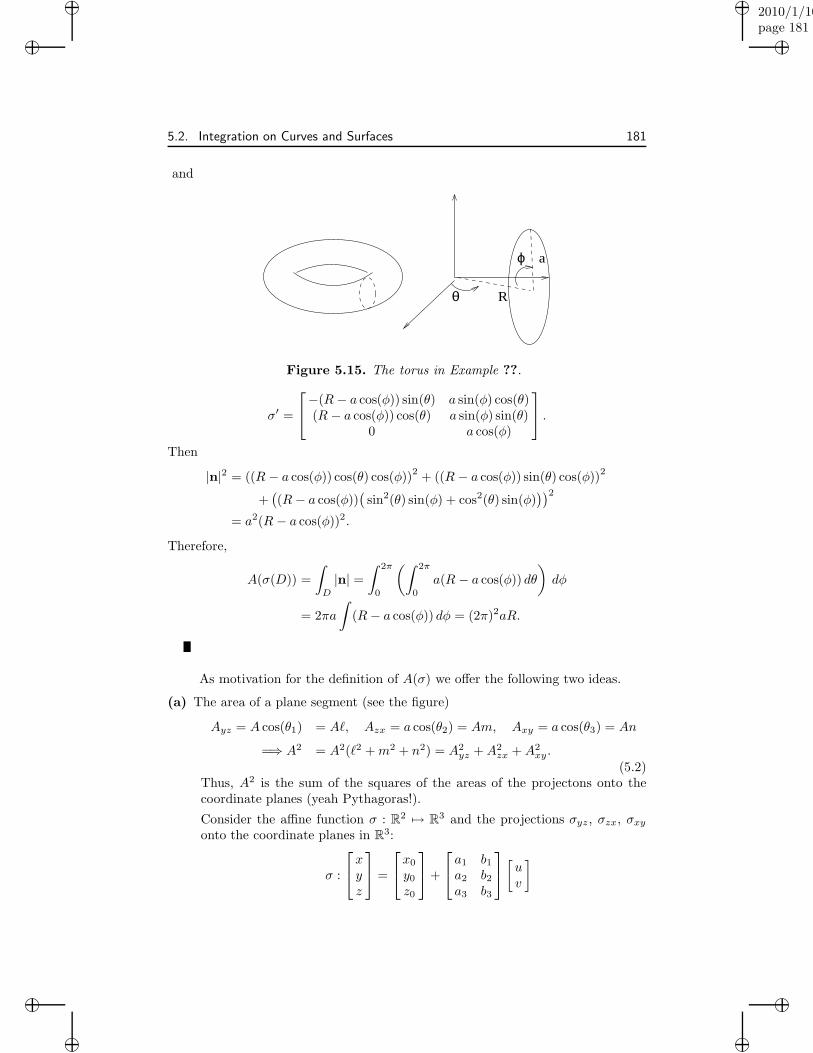
“muldowney”2010/1/10page 181
i
i
i
i
i
i
i
i
5.2. Integration on Curves and Surfaces 181
and
R
a
θ
ϕ
Figure 5.15. The torus in Example ??.
σ′ =
−(R− a cos(φ)) sin(θ) a sin(φ) cos(θ)(R − a cos(φ)) cos(θ) a sin(φ) sin(θ)
0 a cos(φ)
.
Then
|n|2 = ((R − a cos(φ)) cos(θ) cos(φ))2 + ((R − a cos(φ)) sin(θ) cos(φ))2
+((R− a cos(φ))
(sin2(θ) sin(φ) + cos2(θ) sin(φ)
))2
= a2(R − a cos(φ))2.
Therefore,
A(σ(D)) =
∫
D
|n| =∫ 2π
0
(∫ 2π
0
a(R − a cos(φ)) dθ
)dφ
= 2πa
∫(R− a cos(φ)) dφ = (2π)2aR.
As motivation for the definition of A(σ) we offer the following two ideas.
(a) The area of a plane segment (see the figure)
Ayz = A cos(θ1) = Aℓ, Azx = a cos(θ2) = Am, Axy = a cos(θ3) = An
=⇒ A2 = A2(ℓ2 +m2 + n2) = A2yz +A2
zx +A2xy.
(5.2)Thus, A2 is the sum of the squares of the areas of the projectons onto thecoordinate planes (yeah Pythagoras!).
Consider the affine function σ : R2 7→ R3 and the projections σyz, σzx, σxyonto the coordinate planes in R3:
σ :
xyz
=
x0
y0z0
+
a1 b1a2 b2a3 b3
[uv
]
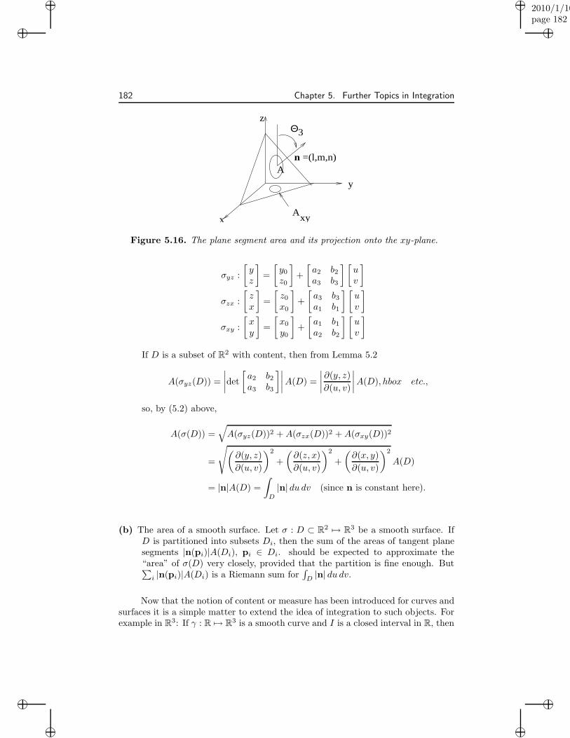
“muldowney”2010/1/10page 182
i
i
i
i
i
i
i
i
182 Chapter 5. Further Topics in Integration
Θ
A
Ax
y
z
xy
3
n =(l,m,n)
Figure 5.16. The plane segment area and its projection onto the xy-plane.
σyz :
[yz
]=
[y0z0
]+
[a2 b2a3 b3
] [uv
]
σzx :
[zx
]=
[z0x0
]+
[a3 b3a1 b1
] [uv
]
σxy :
[xy
]=
[x0
y0
]+
[a1 b1a2 b2
] [uv
]
If D is a subset of R2 with content, then from Lemma 5.2
A(σyz(D)) =
∣∣∣∣det
[a2 b2a3 b3
]∣∣∣∣A(D) =
∣∣∣∣∂(y, z)
∂(u, v)
∣∣∣∣A(D), hbox etc.,
so, by (5.2) above,
A(σ(D)) =√A(σyz(D))2 +A(σzx(D))2 +A(σxy(D))2
=
√(∂(y, z)
∂(u, v)
)2
+
(∂(z, x)
∂(u, v)
)2
+
(∂(x, y)
∂(u, v)
)2
A(D)
= |n|A(D) =
∫
D
|n| du dv (since n is constant here).
(b) The area of a smooth surface. Let σ : D ⊂ R2 7→ R3 be a smooth surface. IfD is partitioned into subsets Di, then the sum of the areas of tangent planesegments |n(pi)|A(Di), pi ∈ Di. should be expected to approximate the“area” of σ(D) very closely, provided that the partition is fine enough. But∑
i |n(pi)|A(Di) is a Riemann sum for∫D |n| du dv.
Now that the notion of content or measure has been introduced for curves andsurfaces it is a simple matter to extend the idea of integration to such objects. Forexample in R3: If γ : R 7→ R3 is a smooth curve and I is a closed interval in R, then
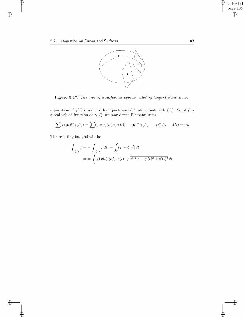
“muldowney”2010/1/10page 183
i
i
i
i
i
i
i
i
5.2. Integration on Curves and Surfaces 183
..
.
Figure 5.17. The area of a surface as approximated by tangent plane areas.
a partition of γ(I) is induced by a partition of I into subintervals {Ii}. So, if f isa real valued function on γ(I), we may define Riemann sums
∑
i
f(pi)ℓ(γ(Ii)) =∑
i
(f ◦ γ)(ti)ℓ(γ(Ii)), pi ∈ γ(Ii), ti ∈ Ii, γ(ti) = pi.
The resulting integral will be
∫
γ(I)
f = =
∫
γ(I)
f dℓ :=
∫
I
(f ◦ γ)|γ′| dt
= =
∫
I
f(x(t), y(t), z(t)
)√x′(t)2 + y′(t)2 + z′(t)2 dt.