Advance Refundings of Municipal Bonds∗

(Preliminary and Incomplete)

Andrew AngColumbia Business School

and NBER

Richard C. GreenTepper School of BusinessCarnegie Mellon University

and NBER

and

Yuhang XingJones Graduate School of Management

Rice University

May 26, 2013

∗We greatly appreciate the research assistance of Karthik Nagarajan, Yunfan Gu, and TsuyoshiSasaki. Tal Heppenstall of University of Pittsburgh Medical Center, Rich Ryffel of Edward Jones,and Paul Luhmann of Stifle Financial provided information about advanced refunding.

Abstract

Municipal bonds are often “advance refunded.” Bonds that are not yet callable aredefeased by creating a trust that pays the interest up to the call date, and pays the callprice. New debt, generally at lower interest rates, is issued to fund the trust. If there is nouncertainty and no fees, the transaction has zero net present value relative to the alternativeof waiting to refund the bonds at the call date. Interest expense is reduced before the calldate in exchange for higher payments afterwards. Effectively, the issuer is able to borrowagainst future interest savings to fund current operating activities. If there is uncertainty(or fees) advance refunding is negative net present value. The issuer pre-commits to call andprovides free credit enhancement. We examine the practice empirically for a large sampleof pre-refunded bonds. We estimate the option value destroyed and the amount of implicitborrowing the transaction affords.

1 Introduction

New issues of municipal bonds in recent years have varied between $300 and $400 billion

a year. In 2012 volume grew by 31%. A total of $376 billion of bonds were issued versus

$288 billion in 2011. This increase was not due to increased investment activities on the part

of municipal issuers. Only $144 billion of this volume was “new money,” bonds that were

issued to fund new investment projects.1 This was actually a slight decrease from 2011. The

rest went to refund existing debt, because the bonds matured, were called, or were “advance

refunded.” According to the leading trade publication, The Bond Buyer, “Low rates fueled

the refunding boom. The triple-A 10-year yield reached historic lows in 2012.”2

In an advance refunding, the municipality issues new debt at a lower interest rate than

existing bonds which are not yet callable, but will be callable in the future. The proceeds

from the new debt fund a trust that covers the remaining coupon payments on the bonds,

along with the call price. The assets in the trust are generally State and Local Government

Securities, or SLUGS, issued by the Treasury specifically for this purpose. This prevents the

issuer from earning the (taxable) rate on assets funded by tax-exempt municipal debt, while

also providing inexpensive financing for the Treasury. The transaction typically lowers the

issuer’s interest cost between the pre-refunding date and the date at which the bonds can

be called.

The practice of advance refunding, or “pre-refunding,” outstanding bonds that are not

yet callable is widespread in the municipal finance. Figure 1 shows par value amounts of

different categories of municipal bond redemptions, by year. The figure shows the par value

of municipal bonds that are retired at maturity, either because they were never callable or

because the call was never exercised. Also shown are bonds that are called during the time

1These figures were reported in The Bond Buyer’s 2012 in Statistics Annual Review, February 11, 2013.2“Refunding Rage Fuels 31% Bounce in Muni Debt,” The Bond Buyer’s 2012 in Statistics Annual Review,

February 11, 2013, p. 2A.

1

period when the call provision is in effect, in a so called “current refunding.” The third

category of bond redemptions in the figure are bonds that are called after having previously

been defeased through an advance refunding. In 2012, for example, $450 billion of municipal

debt was extinguished through redemption (including $53 billion in maturing notes, not

shown in the figure). Of this total, $76.5 billion were bonds that were called after having

previously been pre-refunded. In the early years of the last decade, more pre-refunded bonds

were called than non pre-refunded bonds. In recent years the volume of called, pre-refunded

bonds has been about half of the volume of current refundings.

Advance refunding provides short-term budget relief, but it destroys value for the issuer.

By pre-committing to call, the issuer surrenders the option not to call should interest rates

rise before the call date. The value lost to the issuer, and transferred to bondholders, is the

value of a put option on the bonds. In addition, since the assets in the trust are Treasury

securities, the transaction provides free credit enhancement for the bondholders, also at the

expense of the issuer. Finally, the intermediaries who create the trust and issue the new

bonds collect fees to do so. Payment of these fees would be delayed if the issuer waited to

refund at the call date, and, since pre-refundings do not extend the maturity of the debt,

would be avoided altogether if at the call date the call option were ultimately not exercised.

Indeed, underwriters and traders are known to jokingly refer to advance refundings as “de-

fees-ance.”

Why, given the costs, do municipal issuers pre-refund their bonds? Almost all munici-

palities are required by statutes, charters, or state constitutions to balance their operating

budgets. They can only borrow for capital projects. They are rarely restricted from refund-

ing or pre-refunding existing debt, however, as long as the maturity is not increased. As

we show in the next section, advance refunding allows the municipality to, in effect, borrow

against future potential interest savings. Current interest expense, which is paid out of the

operating budget, is reduced, while future payments after the call date are increased. Ignor-

2

ing the option value lost and credit enhancement provided, the transaction is effectively a

swap, with zero net present value.

Thus, an advance refunding may help the issuer avoid the need to increase parking rates or

to lay off teachers and police. These may be a laudable, even urgent, priorities. Nevertheless,

the restrictions on borrowing to fund these priorities are presumably in place for equally

commendable reasons, which are evidently being circumvented. advance refundings could

be viewed as a non-transparent means of borrowing to fund operating activities. Advance

refundings, by accelerating interest savings at the expense of future savings, can obviously

also help elected officials defer cost cutting or tax increases in an election year.

In this paper, we describe the effects pre-refunding has on cash flows and on the present

value of the issuer’s obligations. advance refunding a bond has two effects. It destroys value

for the issuer, because the issuer pre-commits to call. It also accelerates the realization of

anticipated future interest savings, effectively borrowing against them. Thus, while it allows

issuers to circumvent restrictions on borrowing to fund operating expenses, it does so at

the expense of present value. We then empirically examine the extent of the practice and

quantify its consequences. For a sample of almost 150 thousand pre-refunded bonds, we

estimate the value that is destroyed by pre-refunding and the value of accelerated interest

savings, or implicit borrowing, by issuers.

Advance refundings have received very limited attention in the academic literature. In

an unpublished note, Dammon and Spatt (1993) describe the transaction and explain how

it destroys option value for the issuer. Analyses in specialized journals aimed at practition-

ers often acknowledge that option value is lost, but generally prescribe comparing this loss,

along with fees paid, to the interest savings over the remaining time to maturity. For exam-

ple, Kalotay and May (1998) or Kalotay and Abreo (2010) advocate calculating “refunding

efficiency,” the ratio of the present value of interest savings over the life of the newly issued

debt to the lost option value. Guidelines issued by states implicitly compare the option value

3

to the interest savings by, for example, requiring greater percentage interest savings when

there is a longer time to call. We argue, by contrast, that the interest savings over the life of

the debt are a misleading measure, since waiting to call at the call date and then refunding

is generally the relevant alternative.

The paper is organized as follows. The next section illustrates the cash flow and valuation

effects of advance refundings. Section 3 describes the data and provides descriptive evidence

on pre-refundings and the pervasiveness of the practice. Section 4 evaluates the quantitative

consequences of pre-refunding. It describes the methods we use to price the option value

destroyed through the transaction for the issuers, and provides estimates for the advance

refundings in our sample. We also estimate the present value of interest savings that are

accelerated through time by means of the transaction. Section 5 summarizes and concludes.

2 The Pre-Refunding Decision

This section illustrates the effects advance refunding has on the value of the issuer’s liability,

and on the pattern of cash flows associated with that liability through time.

2.1 Present Value Effects

Suppose the price of a bond at date t is Vt. The bond is callable at an exercise price of

$K at date τ and matures at date T > τ > t. It pays a continuous coupon at rate c. We

consider the simplest case of a one-time opportunity to pre-refund the bond at the current

date of t, and a single opportunity to call at date τ . That is, we treat the call provision as

a European option. The cost of early exercise for this case is a conservative estimate of the

cost. It ignores the value of delaying exercise further, after the call date, but that option is

also foregone through a commitment to call in a pre-refunding.

The consequences of credit risk on present values are obvious, though difficult to quantify

4

theoretically and empirically, so we ignore them here. Keep in mind that the credit risk for

most of the municipal sector has been quite low in modern times compared to the corporate

sector—recent fiscal problems at the state and local level notwithstanding.

Let Vτ be the present value of the coupon stream between the call date and maturity. Let

r(s) denote the instantaneous riskless rate prevailing at date s. We can represent the value

of any security as the discounted expectation of its payoffs under the risk-neutral measure.

Vτ = E∗τ

{∫ T

τ

ce−∫ sτ r(v)dvds+ 1e−

∫ Tτ r(v)dv

}.

where E∗τ (·) denotes the risk-neutral expectation conditional on information available at date

τ .

Consider, then, two alternatives:

1. Wait until the call date and then decide whether to call and refund the bonds.

2. Advance refund the bonds at the current date, t.

The payoffs up to the call date are the same in either case. If it waits to call, the issuer pays

the coupon until the call date. If the issuer pre-refunds the bonds, the old debt is defeased,

but new debt must be issued to fund the trust making the payments up to the call date.

The issuer’s liability at the call under the first alternative is min{K,Vτ}. Under the second

alternative, the advance refunding, the issuer must pay K unconditionally. The difference is

then:

K −min{K,Vτ} = max{K − Vτ , 0}.

This is the payoff on a put option on the bond. The present value of this put is the option

value transferred from the issuer to the bondholders by the advance refunding. Thus, the

5

value of the issuer’s liability today, if the bond is not pre-refunded will be,

Lt = E∗t

{∫ τ

t

ce−∫ st r(v)dvds+ min{K,Vτ}e−

∫ τt r(v)dv

}.

The issuer’s liability under a pre-refunding will be:

L̂t = E∗t

{∫ τ

t

ce−∫ st r(v)dvds+Ke−

∫ τt r(v)dv

}.

The difference between these, L̂t − Lt, is the value that is destroyed for the issuer by the

advance refunding for the issuer. Evidently,

L̂t − Lt = E∗t

{max{K − Vτ , 0}e−

∫ τt r(v)dv

},

the value of a put option on the coupon bond exercisable on the call date.

2.2 Cash Flow Effects

Given that it is obvious from the above that value is destroyed for the issuer by the pre-

refunding, why do issuers engage in this practice? The new debt that is issued to fund the

trust will generally have a lower interest rate than does the old debt, as long as interest

rates have fallen between the advanced-refunding date and the date when the bonds were

originally issued. The lower rate does contribute to the municipality’s operating budget.

We can illustrate these effects with a simple example. Suppose the term structure is

flat at all points, and, again, ignore any default risk. To keep the exposition simple, we

will assume coupon payments are made annually. A municipal entity has previously issued

bonds with $100 face value and a 6% coupon. Interest rates have since fallen to 4%. There

are 6 years to maturity, and the bonds are callable at $100 the end of 3 years. Let us first

abstract from the optionality in the call provision for the bonds, and assume it is known

6

with certainty that rates will remain at 4% forever.

If the bonds were callable at the current date, the decision would be easy. The munic-

ipality would issue new bonds with 6 years to maturity and refund the old bonds. Their

annual interest payments per $100 par value would drop from $6 to $4, and the present value

of these savings would be:

2

.04

(1− 1

1.046

)= $10.48

per $100 of face value.

Unfortunately, the bonds are not immediately callable, and the issuer must choose be-

tween waiting three years to call or pre-refunding now. If the issuer waits the three years

to call the bonds its pays $6 for three years, and the strike price at the end of three years,

financed by issuing a new 3-yr bond at 4%. The payments over the six-year horizon, the

interest savings, and their present values are given in rows two and three of Table 1.

If the issuer pre-refunds it must issue a 6-year bond at a coupon rate of 4% sufficient to

fund the payments over the next three years and the call price. The face value of the bond

must be

6

.04

(1− 1

1.043

)+

100

1.043= 105.55

The coupon payments on the new bonds will be:

105.55 ∗ 0.04 = 4.22

The interest savings associated with pre-refunding are in rows 4 and 5 of Table 1.

Notice that, because we are assuming certainty about future rates, the present values of

the interest savings under the two alternatives are equal. Only the timing of the interest

savings differs. The final line in the table shows the savings associated with pre-refunding less

the savings associated with waiting to call. The pre-refunding accelerates the interest savings

7

at the expense of higher interest payments over the later years, and an higher payment at

maturity.

The present values of the positive and negative flows in the last line are equal. The issuer

is effectively borrowing against future interest savings associated with the opportunity to call,

as well as a higher principle repayment, to reduce interest expense now. The present value

of the accelerated interest savings, $4.95 per $100 face value, is achieved by surrendering

the same present value of savings later. Alternatively, the issuer could achieve the payment

stream associated with pre-refunding by entering a swap contract that paid the municipality

$1.78 each year for three years, in exchange for the promise to pay $0.22 annually starting

in year four, augmented by $5.55 in year six. It has zero present value at the current date,

but effectively borrows over the first three years in exchange for payments over the last three

years.

Evidently then, under certainty about the evolution of future interest rates, waiting to

refund, versus pre-refunding has no effect of the present value of the issuer’s liability. Why

then would an issuer want to do this? When pre-refunding, the issuer has interest expense

each period between the $6 associated with the existing debt and the $4 it will pay after the

call date if it waits to call. Though this has no effect on the present value of the issuer’s

liabilities, it may very well affect its freedom to spend money or reduce taxes. Municipalities

can only borrow to fund capital projects, and even then there are often elaborate restrictions

(or safeguards), such as requiring approval of voters or a state-wide board for a new bond

issue. There are generally no such restrictions associated with refunding activities, however,

so long as they do not extend the maturity of the original debt.

2.2.1 Uncertainty

To this point, in our example the pre-refunding is neutral in terms of present value. Suppose,

however, that there is some possibility interest rates will rise over the next three years above

8

the 6% rate on the existing debt. Then the precommitment to call must be destructive of

value, because it forces the firm to call even when it is suboptimal to do so.

When there is uncertainty about future rates, the interest savings that will eventually

be realized by waiting to call are uncertain, and thus so are the differences through time

associated with an advanced versus a (delayed) current refunding. Indeed, surely part of the

appeal of pre-refunding is confusion about the need to engage in the practice to “lock in”

interest savings that would otherwise be lost should rates rise before the call date. If the goal

is to hedge this uncertainty, then a variety of hedging strategies could achieve this without

precommitting to call. Even if the goal is to accelerate or borrow against the uncertain

future interest savings associated with the call provision, a swap contract could achieve

this more efficiently. If we denote the uncertain three year interest rate that will prevail

three years from now as r̃3 percent, then the interest payments from years 4-6 associated

with waiting to call are min{6, r̃3}. The issuer could arrange to swap some portion of this

liability for cash payments of equal present value over the first three years. Of course, such a

step would be more transparent as “borrowing” to the public or to any governmental entity

supervisorial authority, and thus might be politically or legally infeasible. This raises the

question, however, of why the issuer should be permitted to borrow in an opaque manner

that destroys value when doing so directly and transparently would not be allowed.

2.3 Urgency

Consideration of a specific example may provide some sense of the political context in which

advance refundings are carried out. In the spring of 2005 the city of Pittsburgh, Pennsylvania,

faced some very difficult choices. The city’s debt had accumulated to $821 million in gross

bonded debt representing $2,456 owed for every person living in the city. Debt service

9

amounted to a quarter of spending by the city.3 A state board had been appointed under

state law to oversee the city’s finances. The administration of Mayor Tom Murphy, in a

desperate effort to balance the 2004 budget, had accelerated revenues and deferred expenses.

Revenue shortfalls relative to that budget were $7 million, and expenses exceeded the budget

by $13 million, depleting the city’s cash reserves. The city council found itself with no

funds available for continuing maintenence on the city streets, and the mayor had previously

pledged not to increase the city’s debt any further.

At this point, the city council debated two proposals aimed at generating funds for road

maintenance.4 Mayor Murphy’s proposal involved advance refunding roughly $200 million

of city bonds that had been issued in 1995 and 1997. Their maturities ranged from one to

thirteen years. The 1995 bonds would otherwise have been callable in September of 2005,

or in roughly four months. The 1997 series would otherwise have been callable in August of

2007. The transaction would, after $2.4 in fees, contribute $6 million in funds over the next

year for street resurfacing and “fixing potholes.” The alternative, offered by the chairman of

the Council’s Finance Committee, Doug Shields, was to borrow $5 million from a regional

development authority for one year, with interest and fees of $164,000.

The fees for the advance refunding included approximately $1.86 million for bond insur-

ance, $1 million to the underwriters, Lehman Brothers and National City, and $370 thousand

for the bond counsel and underwriter’s attorneys.

After two hours of debate, the city council voted 6 to 2 for the advanced refunding.

Proponents of the mayor’s plan argued it did not require the city to increase its debt.

Councilman Udin declared, “The $6 million is free money. I think it would be a mistake to

leave $6 million on the table.” Afterwards, the mayor’s spokesman explained, “The mayor

3Pittsburgh Post-Gazette “City’s Debt Looms: Large Principal and Interest Now 25% of Spending,” April30, 2005.

4Details and quotations from Pittsburgh Post-Gazette “Council OKs Bond Refinancing Plan Will FundPaving, Other Work,” April 7, 2005.

10

made a commitment that he would not increase the city’s debt this year, and the Shields

plan obviously would have done that.”

3 Data Sources and Descriptive Statistics

We draw data from several sources. We obtain transaction data for municipal bonds from the

Municipal Securities Rule Making Board (MSRB). This database includes every trade made

through registered broker-dealers, and identifies each trade as a purchase from a customer,

a sale to a customer, or an interdealer trade. We augment this with data from Bloomberg

that includes information about the refunding status of the bonds.

Over our sample period from January 1995 to December 2009, the MSRB database

contains 95,162,552 individual transactions involving 2,516,534 unique municipal securities,

which are identified through a CUSIP number. The MSRB database contains only the

coupon, dated date of issue, and maturity date of each security. We obtain other issue

characteristics for all the municipal bonds traded in the sample from Bloomberg. Specifically,

we collect information on the bond type (callable, putable, sinkable, etc.); the coupon type

(floating, fixed, or OID); the issue price and yield; the tax status (federal and/or state

tax-exempt, or subject to the Alternative Minimum Tax (AMT); the size of the original

issue; the S&P rating; whether the bond is insured; and information related to advance

refunded municipal bonds. The information on advance refunded municipal bonds includes

an indicator of whether the bond is a pre-refunded bond, the pre-refunded date, the pre-

refunded price, and the escrow security type.

Pre-refunded municipal bonds are collateralized by some of the safest securities available.

The most common types of collateral used are: U.S. Treasury Securities; State and Local

Government Securities (SLGS); U.S. Agency Securities: FNMA, FHLMC, TVA, HUD and

FHA ; Aaa/AAA rated Guaranteed Investment Contracts (GICS). Among them, SLUGS

11

are a form of U.S. Treasuries created explicitly for municipalities to use for debt refinancing

purpose.

Among the 2,516,534 unique cusips, 258,822 are identified by Bloomberg as pre-refunded

bonds with a total par value of 886,478,744,590 dollars. We apply for following data filter

for our analysis. We focus on pre-refunded bonds that are exempt from federal and state

income taxes and are not subject to the AMT. This reduces our sample to 245,184 bonds.

We take only pre-refunded bonds with the following escrow security type: U.S. Treasury

Securities; SLGS; and cash. This reduces our sample to 237,703. We also limit our bond

universe to bonds issued in one of the 50 states, and so we exclude bonds issued in Puerto

Rico, the Virgin Islands, other territories of the U.S. such as American Samoa, the Canal

Zone, and Guam. After this filter, we have 237,660 bonds. We require bonds to have

non-missing information on when they became pre-refunded and this left us 158,477 bonds.

And finally, we require all bonds to have non-missing coupon rate, fixed coupon rate only

with semi-annual coupon payment, non-missing information on call date, call price, proper

information on CUSIP and delete obvious data errors and our final sample contains 148,961

bonds.

The sum of par value in our final sample is 454,377,469,426 dollars, which is about 51.25%

of total aggregate par amount of pre-refunded bonds. Thus, our estimates of the aggregate

impact of these transactions is clearly conservative. As we shall see, however, most of the loss

in option value is associated with a relatively small fraction of the pre-refundings with very

large par value. These large deals are presumably less likely to have missing data associated

with them.

We wish to price the options on coupon bonds, which are the primary source of the value

lost through pre-refunding, and also to evaluate the present values of interest savings to the

call date, which represents the borrowing implicit in the refunding. For these purposes we

require information on the term structure for tax-exempt bonds. We follow Ang, Bhansali

12

and Xing (2010) and use zero-coupon rates inferred from transactions prices on municipal

bonds in the MSRB database. These zero-coupon yield curves are constructed using the

Nelson and Siegel (1987) method, fit each day in the sample period to interdealer prices.

Details are provided in the internet appendix to Ang, Bhansali and Xing (2010).

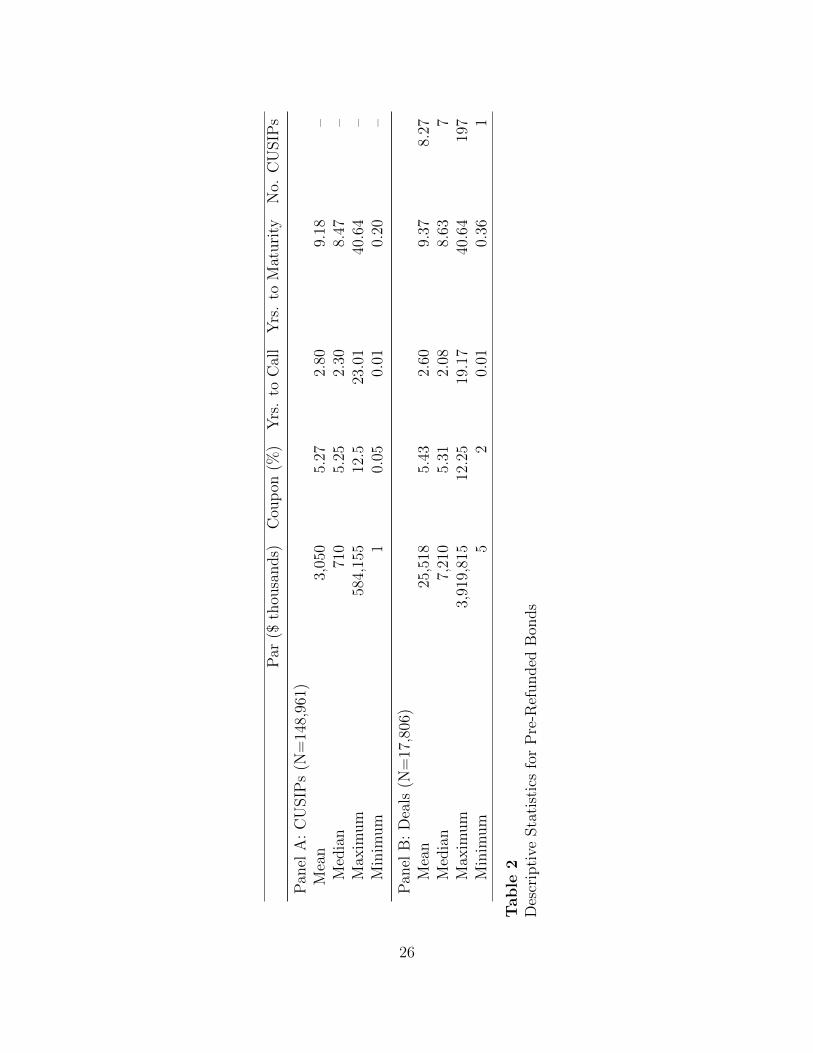
Table 2 provides descriptive statistics covering all the pre-refundings in our dataset,

treating the unit of observation as the CUSIP and as the “deal.” We define a deal as any

set of bonds from the same issuer that become pre-refunded on the same date. The average

CUSIP that is advance refunded involves just over $3 million in par value, though the lower

median suggests skewness in the size of pre-refundings. The smallest CUSIPs that were

pre-refunded were issued by small health care facilities and school districts. The largest were

New Jersey Tobacco Settlement Bonds, the Los Angeles Unified School District, Long Island

Power, and the Tri-Borough Bridge and Tunnel Authority. All of these were pre-refunded

2-5 years before they became callable.

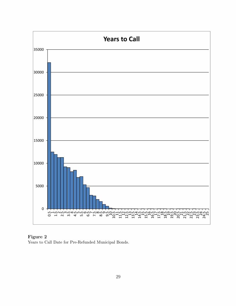
The average time to call is 2.8 years. The distribution of time to call is of particular

importance in evaluating the financial implications of the advance refundings. If the only

bonds being pre-refunded are bonds that are about to be called in any case, not much option

value is being lost. Figure 2 suggests this is often the case. Over 32,000 of the roughly 150,000

pre-refunded CUSIPs have less than six months to call. There are substantial numbers

(35,379) of pre-refunded bonds with five or more years to call, however, and small numbers

(306) with ten or more years to call.

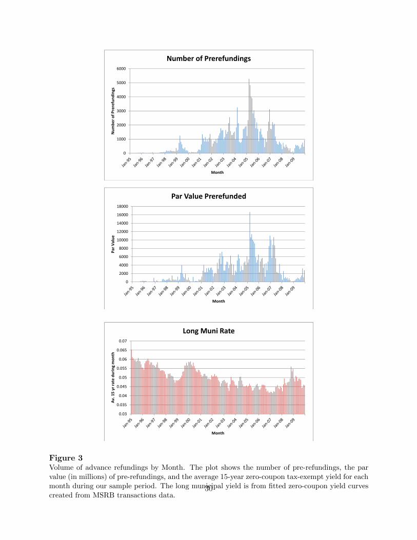
Figure 3 shows the number of advance refundings, the par value of advance refundings,

and the average 15-year municipal bond yield, by month, in our sample. The volume of

pre-refunding activity clearly rises as interest rates fall, though evidently with something of

a lag. Activity peaked in 2005, and slowed when municipal credit spreads rose in response

to the credit crisis of 2007-2008 and the collapse of the major bond insurance firms, on

which the municipal market was heavily dependent. Over the most recent period, since

13

our sample ended, municipal credit spreads have fallen and long-term interest rates have

achieved historic lows. As we noted in the introduction, press reports suggest this has led

to a revival of advance refunding activity.

4 Quantitative Consequences of pre-refundings

It should be clear from the analysis above that advance refundings destroy value for the issuer,

but allow the issuer to borrow against expected future interest savings. How much value is

destroyed in the typical deal, in aggregate, and in the worst deals? How much “borrowing” is

going on? In this section we take some preliminary steps towards a quantitative assessment

of these questions.

4.1 Lost Option Value

First, we provide estimates of the value lost to issuers from the precommitment to call in

pre-refundings. This requires that we calculate, for each pre-refunded bond, the value of a

put option exercisable at the call price and call date on a coupon bond. The single-factor

Vasicek (1977) model provides a particularly simple means of doing this, although it has

well-known limitations. In the Vasicek setting, the value of an option on pure-discount bond

can be expressed in closed form. The method of Jamshidian (1989) can then be used to price

options on coupon bonds. Since a coupon bond can be viewed as a portfolio of pure-discount

bonds, and since the prices of all zero-coupon bonds are monotonic in the the short-term

rate for a single-factor model, the value of an option on a coupon bond can be expressed

as a portfolio of options on the zero-coupon components, each with an appropriately chosen

exercise price. While this approach provides a rough idea of the magnitudes involved, our

intention in future versions of this paper is to implement a two-factor model that, while

necessitating numerical solution methods, can provide more realistic estimates.

14

We assume that the underlying call option on the bond is a European option, and that

the decision to pre-refund is made at a single point in time. In both cases, these assumptions

would lead our estimates of the lost option value to be conservative.

The Vasicek (1977) model assumes the short interest rate is Gaussian and mean-reverting:

dr(t) = κ(θ − r(t))dt+ σdW (t)

where W (t) is a Brownian motion. Under the risk-neutral measure, the short rate follows

dr(t) = κ(θ̄(t)− r(t))dt+ σdW (t)

where

θ̄(t) = θ − σλ(t)

κ.

We assume the market price of risk is linear in the short rate:

λ(t) = λ0 + λ1r(t).

The yield on a bond maturing in τ periods can then be written as linear functions of the

short rate:

z[r(t), τ ] = −A(t, τ)

τ+B(τ)

τr(t),

where

B(τ) =1

κ(1− e−κτ ),

A(t, τ) =γ(t)(B(τ)− τ)

κ2− σ2B(τ)2

4κ,

and

γ(t) = κ2θ̄(t)− σ2

2.

15

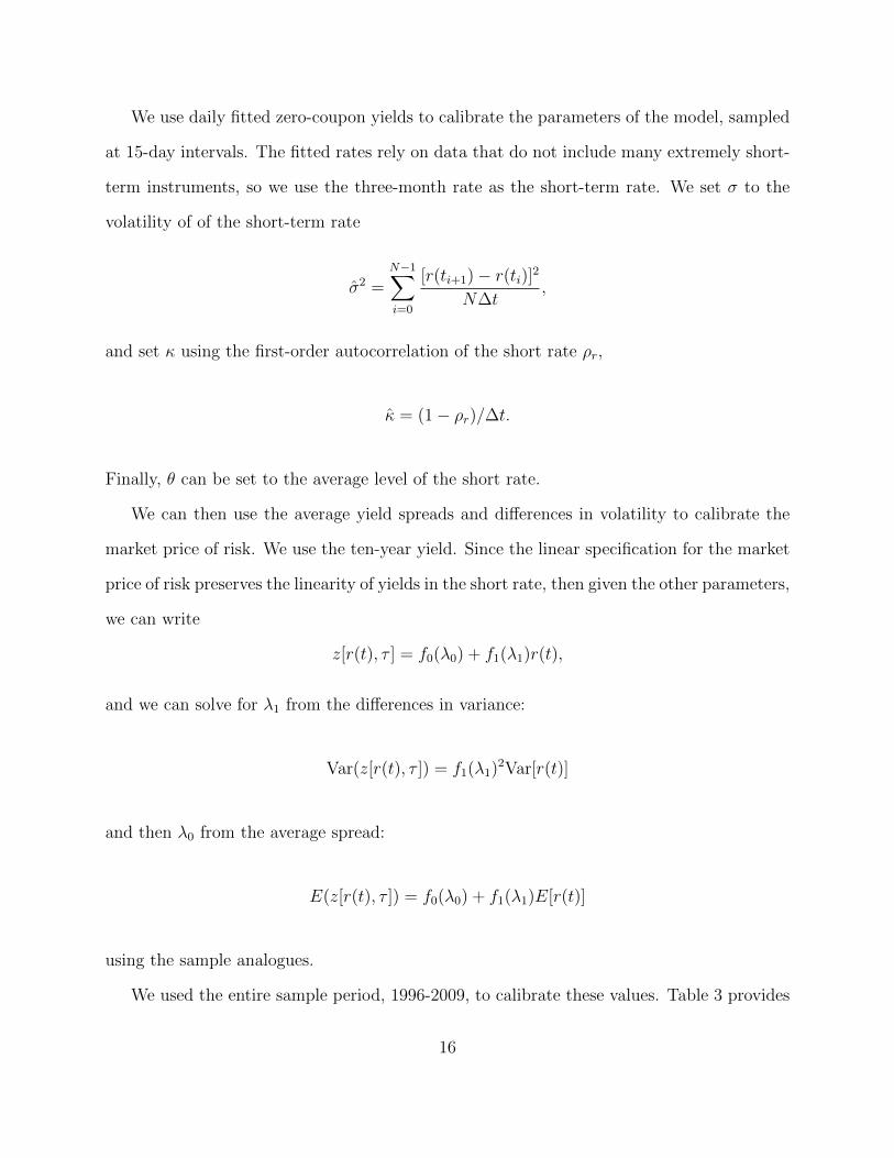
We use daily fitted zero-coupon yields to calibrate the parameters of the model, sampled

at 15-day intervals. The fitted rates rely on data that do not include many extremely short-

term instruments, so we use the three-month rate as the short-term rate. We set σ to the

volatility of of the short-term rate

σ̂2 =N−1∑i=0

[r(ti+1)− r(ti)]2

N∆t,

and set κ using the first-order autocorrelation of the short rate ρr,

κ̂ = (1− ρr)/∆t.

Finally, θ can be set to the average level of the short rate.

We can then use the average yield spreads and differences in volatility to calibrate the

market price of risk. We use the ten-year yield. Since the linear specification for the market

price of risk preserves the linearity of yields in the short rate, then given the other parameters,

we can write

z[r(t), τ ] = f0(λ0) + f1(λ1)r(t),

and we can solve for λ1 from the differences in variance:

Var(z[r(t), τ ]) = f1(λ1)2Var[r(t)]

and then λ0 from the average spread:

E(z[r(t), τ ]) = f0(λ0) + f1(λ1)E[r(t)]

using the sample analogues.

We used the entire sample period, 1996-2009, to calibrate these values. Table 3 provides

16

the parameter values we calibrated in this manner, along with alternative values based on

subperiods. The long-run mean, θ, is quite sensitive to sample period employed, since this

was a period of gradually declining interest rates. (See the third panel of Figure 3.) The

estimates of the option values we obtain are, in turn, quite sensitive to the value of θ we

choose. This is not surprising. If current rates, and expectations about future rates, are

low relative to the historical average over the sample period, our estimates of the put option

values will be misleading, although the direction of the effect may depend on the strength

of the mean-reversion parameter.

In subsequent versions of this work we hope to augment these estimates of the option

values with those from a two-factor model. The great advantage of a single-factor model in

this context is that it allows us to compute option values for coupon bonds directly.

Under the Vasicek model, options on zero-coupon bonds have known closed-form solu-

tions. An option on a coupon bond, however, can be viewed as an option on a portfolio of

zero-coupon bonds. Suppose there are N payments remaining after the exercise date for the

option, and these occur at times (measured current date), τi, i = 1, . . . , N . Then we can

write the value of the bond as function of the short rate as

V [r(t)] =N−1∑i=1

CP [r(t), τi] + [100 + C]P [r(t), τi]

Note that each zero-coupon bond price, P [r(t), τi] is monotonic in the short rate under the

Vasicek (or any other single-factor) model. Therefore, as Jamshidian (1989) shows, we can

define a critical interest rate r∗ such that V [r∗] = K: the value of the coupon bond equals

the stike price. Now define Ki ≡ P (r∗, τi). We know by monotonicity that V [r(t)] > K if

and only if P (r∗, τi) > Ki, for all i. Thus, we can treat the option on the coupon bond as a

portfolio of options on the zeroes, each with an appropriately chosen exercise price. It is a

simple matter to find r∗ iteratively. It can then be used to find Ki for each coupon maturity,

17

τi. The value of each option on each zero can then be computed using the known close-form

solution, and the value of the option on the coupon bond is the sum of these options on the

zeroes times the payments at those dates.

We applied this procedure to each of the 148,961 separate CUSIPS that were pre-refunded

during our sample period and for which we have the variables needed to perform the cal-

culations. Recall that the option value that is lost by committing to call before the call

date is the value of a put option on the coupon bond expiring on the call date. Table 4

provides summary information the distribution of the put-option values: the value destroyed

per $100 face value and the total value destroyed for each CUSIP and deal. As is evident

from the large differences between the means and medians, these distributions are extremely

skewed for both CUSIPs and deals. The vast majority of advance refundings are relatively

innocuous in terms of the option value surrendered. The call option is deep in the money

and/or the bond is relatively close to the call date. There are some very large and very

bad deals, however. On July 7, 2005, the Triborough Bridge and Tunnel Authority advance

refunded four bonds. One of these was the largest pre-refunded bond in our sample by par

value, $584,155,000. Our estimates suggest refunding it also destroyed more value than any

other bond in our sample, $19.9 million. The other three bonds in the deal involved $21.3

million, $36.6 million, and $75.3 million in par value. The put option value for the entire

advance refunding deal was over $21 million. On April 1, 2007, the state of California ad-

vance refunded 135 different CUSIPs. Only one of these had less than a year to call. The

total par value of these bonds was $3.920 billion, and the lost option value to the state is

estimated by our model to be $97 million.

Table 5 shows our estimates of the total value destroyed by the pre-refundings in our

sample, along with some indication of how these numbers change with the parameter values.

In total, the option value surrendered is less than 1% of the par value of the bonds that are

pre-refunded. Since there are a great many bonds, however, the losses total over $4 billion.

18

These estimates are relatively insensitive to the parameters other than the long-run mean, θ.

Most of the value lost is due to a small fraction of the transactions. The pre-refundings that

generate losses in excess of the 95th percentile account for almost $3 billion of the $4 billion

in estimated losses. These tend to be CUSIPs with large par value outstanding, issued by

big public entities. The correlation between issue size and total option value lost is 63% and

the correlation between total value lost and years to call is 12%. The distribution of option

value lost is more skewed than that of issue size. The largest 5% of deals and of CUSIPs

account for 50.23% and 51.70% of total par value in our sample.

There are some smaller pre-refundings that destroy large fractions of the par value re-

funded. Indeed, many of the refundings that have high put option values per $100 face value

would be poor candidates even for a current refunding. For example, on December 14, 2006,

the New Jersey State Education Facility advance refunded two bonds that had originally

been issued at par value with coupons of 3.875%. The bonds would have matured in 2028.

Our estimate of the zero-coupon municipal interest rates for all maturities beyond 10 years

on that date exceed 4%. The bonds were advance refunded along with a large number of

other maturities that had been originally issued in the same offering. Apparently, the issuer

chose to pre-refund the whole series, rather than to selectively pick and choose, despite the

fact that new bonds were being issued at higher rates than some of the bonds being defeased.

In some cases, this may be motivated by bond indentures that apply to the entire series, and

which can only be lifted by pre-refunding all the bonds.

4.2 The Magnitude of Implicit Borrowing

Along with destroying part of the value of the issuer’s call option, advance refunding reduces

interest expense to the issuer immediately at the expense of expected interest savings after

the call date. In effect, the issuer is borrowing against future interest savings. In this section,

we attempt to measure this implicit borrowing.

19

As with the option value destroyed, the amount of borrowing implicit in an advance

refunding will increase with the time to call. As we have seen, the typical bond is pre-refunded

quite close to the call date, and so we would expect both of these quantities to be relatively

small. Unlike the lost call option value, however, the amount of implicit borrowing increases

the more interest rates have dropped since the bonds were issued. In these situations, because

the chances the call will expire out of the money are low, the lost option value is small even

though the amount of implicit borrowing may be significant.

The example in Section 2.2 illustrates that the amount of borrowing against expected

future interest savings is the present value of the difference, up to the call date, between the

coupon on the old debt and the coupon payments on the new debt issued to fund the trust.

The latter will reflect both the lower interest rates on a new par issue and the higher par

value amount required to fund the trust for the remaining payments up to call. Assuming

interest rates have fallen since the original issue date, the old debt will be at a premium, so

the value of the trust exceeds the par amount of the issue.

Given information about the municipal term structure on the date of the advance re-

funding, calculating the amount of implicit borrowing for a given CUSIP or deal would be

straightforward if we could observe the amount put in trust and the coupon rates on the

newly issued debt. For a given CUSIP, this information is available in the official state-

ments (analogous to a prospectus for municipals) associated with the new debt. Formats

are not standardized, however, and the new debt issue may involve purposes in addition to

the advance refunding. In any case, the official statements are available, at best, only as pdf

documents on line. Our large sample of almost 150,000 bonds, precludes gathering this data

by hand.

Accordingly, we attempt to approximate the magnitudes involved using information from

the term structure to estimate the coupon rates at which debt could be issued on the pre-

refunding date. Using the fitted zero-coupon municipal yields, we first calculate the present

20

value of coupon payments that remain until the call date, and of the call price. This we treat

as the size of the trust and the par value of new debt that must be issued to fund it. Let F

denote this funding requirement, per $100 par value. Since typically interest rates will have

fallen, we will generally have F > 100. The same fitted zero-coupon yields can be used to

approximate the coupon on a new par bond with a maturity equal to that of the old bond.

If dt is the zero-coupon price per for a zero that pays $1 in t periods, and the original bond

has T periods to maturity, then the coupon of a par bond solves:

100 = C∗(T∑t=1

dt) + 100dT .

The per period reduction in interest cost is then C − FC∗, where C is the coupon on the

bond being advance refunded. The present value of this difference, up to the call date, times

the total par value outstanding of the pre-refunded issue, is our estimate of the present value

of interest savings that are accelerated, or borrowed, through the transaction.

Table 6 provides summary information about the cross-sectional distribution of the

amount of implicit borrowing associated with the advance refundings. It reports statis-

tics for both individual CUSIPs and deals as the unit of observation. As is the case for lost

option value, the distribution is extremely skewed. This is evident in the dramatic differences

between means and medians for both deals and CUSIPs. The present value of accelerated

interest deductions is only $9,839 for the median CUSIP and $87,876 for the median deal.

The associated means are $48,201 and $403,235, respectively. Most of the implicit borrowing

is associated with a small number of large deals. In total, the advance refundings in our sam-

ple give issuers over $7 billion worth of estimated accelerated interest savings. This is 1.57%

of the par value of pre-refunded bonds. Over 60% of the total, however, comes from only

5% of the CUSIPs or deals. The CUSIP that triggered the most implicit borrowing is a New

Jersey Tobacco Settlement bond that was pre-refunded in January of 2007, one of twelve

21

such CUSIPs in what is also the deal for which implicit borrowing was the largest. The deal

involved $2.163 billion in par value with an average time to call of over five years. This deal

was also in the top one percent in terms of estimated option value lost ($7,911,690). As

noted earlier, however, this need not be the case, because deals for which the call is deep in

the money will involve a large amount of implicit borrowing, but relatively little destruction

of option value. Indeed, while the correlation between implicit borrowing and option value

lost is 21.3% at the deal level, it is slightly negative (-7.9%) when the unit of observation is

the individual CUSIP.

5 Conclusion

The widespread practice of advance refunding of municipal bonds is, at best, zero net present

value, though wasteful of fees. If there is any chance that the bonds would otherwise not be

called, or any risk of default, the transaction destroys value for the issuer. advance refunding

does allow the municipality to realize interest savings prior to the call date, at the expense

of savings that would otherwise be realized afterwards, and this can relieve pressure on

operating budgets. Municipalities are generally prohibited from borrowing to fund operating

activities. advance refunding can be a means of circumventing these restrictions.

Using a large sample of municipal bonds that have been advance refunded, we estimate

both the option value destroyed and the amount of borrowing implicit in the transactions.

For the vast majority of refundings, both quantities are small in either dollar terms or

percentage terms. The distributions of both quantities are highly skewed. Most of the value

destroyed and the largest amount of implicit borrowing is associated with a small fraction

of pre-refundings, typically very large ones.

Our results to this point are preliminary. They use derivative-pricing methods that are

particularly straightforward to implement, although they have well understood deficiencies

22

in capturing the dynamics of interest rates. In future versions of this work we hope to

construct more accurate estimates of the option value lost with more sophisticated models.

Given the underlying patterns of remaining time to call and of the par value of bond issues,

which are also highly skewed, we expect the above conclusions to prove qualitatively robust.

23

References

Ang, Andrew, Vineer Bhansali, and Yuhang Xing, 2010, “Taxes on Tax-exempt Bonds,”

Journal of Finance, 65, 2, 565-601.

Ang, Andrew, Vineer Bhansali, and Yuhang Xing, 2011, Decomposing Municipal Bond

Yields, working paper, Columbia University.

Ang, Andrew and Richard C. Green, 2012, “Reducing Borrowing Costs for States and Mu-

nicipalities Through CommonMuni,” Brookings Institute, Hamilton Project Discussion

Paper 2011-01, February 2011.

Damon, Robert M. and Chester S. Spatt, 1993, “A Note on Advance Refunding of Municipal

Debt,” working paper, Carnegie Mellon University.

Jamshidian, Farshid, 1989, “An Exact Bond Option Formula,” Journal of Finance, 44, 1,

205-209.

Kalotay, Andrew J. and Leslie Abreo, 2010, “Making the Right Call,” Credit, October 2010,

57-59.

Kalotay, Andrew J. and William H. May, 1998, “The Timing of Advance Refunding of

Tax-Exempt Municipal Bonds,” Municipal Finance Journal, Fall 1998, 1-15.

Nelson, Charles R., and Andrew F. Siegel, 1987, “Parsimonious Modeling of Yield Curves,”

Journal of Business, 60, 473-489.

Vasicek, Oldrich, 1977, “An Equilibrium Characterisation of the Term Structure,” Journal

of Financial Economics, 5, 2, 177188.

24

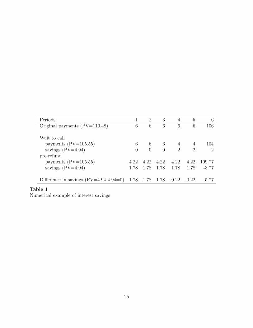
Periods 1 2 3 4 5 6Original payments (PV=110.48) 6 6 6 6 6 106

Wait to callpayments (PV=105.55) 6 6 6 4 4 104savings (PV=4.94) 0 0 0 2 2 2

pre-refundpayments (PV=105.55) 4.22 4.22 4.22 4.22 4.22 109.77savings (PV=4.94) 1.78 1.78 1.78 1.78 1.78 -3.77

Difference in savings (PV=4.94-4.94=0) 1.78 1.78 1.78 -0.22 -0.22 - 5.77

Table 1Numerical example of interest savings

25

Par

($th

ousa

nds)

Cou

pon

(%)

Yrs

.to

Cal

lY

rs.

toM

aturi

tyN

o.C

USIP

s

Pan

elA

:C

USIP

s(N

=14

8,96

1)M

ean

3,05

05.

272.

809.

18–

Med

ian

710

5.25

2.30

8.47

–M

axim

um

584,

155

12.5

23.0

140

.64

–M

inim

um

10.

050.

010.

20–

Pan

elB

:D

eals

(N=

17,8

06)

Mea

n25

,518

5.43

2.60

9.37

8.27

Med

ian

7,21

05.

312.

088.

637

Max

imum

3,91

9,81

512

.25

19.1

740

.64

197

Min

imum

52

0.01

0.36

1

Tab

le2

Des

crip

tive

Sta

tist

ics

for

Pre

-Ref

unded

Bon

ds

26

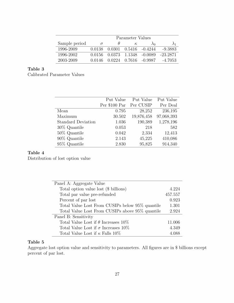
Parameter ValuesSample period σ θ κ λ0 λ11996-2009 0.0138 0.0301 0.5416 -0.4244 -9.38831996-2002 0.0156 0.0373 1.1348 -0.0089 -23.28712003-2009 0.0146 0.0224 0.7616 -0.9987 -4.7053

Table 3Calibrated Parameter Values

Put Value Put Value Put ValuePer $100 Par Per CUSIP Per Deal

Mean 0.795 28,252 236,195Maximum 30.502 19,876,458 97,068,393Standard Deviation 1.036 190,389 1,278,19630% Quantile 0.053 218 58250% Quantile 0.042 2,334 12,41390% Quantile 2.143 45,225 410,08695% Quantile 2.830 95,825 914,340

Table 4Distribution of lost option value

Panel A: Aggregate ValueTotal option value lost ($ billions) 4.224Total par value pre-refunded 457.557Percent of par lost 0.923Total Value Lost From CUSIPs below 95% quantile 1.301Total Value Lost From CUSIPs above 95% quantile 2.924

Panel B: SensitivityTotal Value Lost if θ Increases 10% 11.006Total Value Lost if σ Increases 10% 4.349Total Value Lost if κ Falls 10% 4.088

Table 5Aggregate lost option value and sensitivity to parameters. All figures are in $ billions exceptpercent of par lost.

27

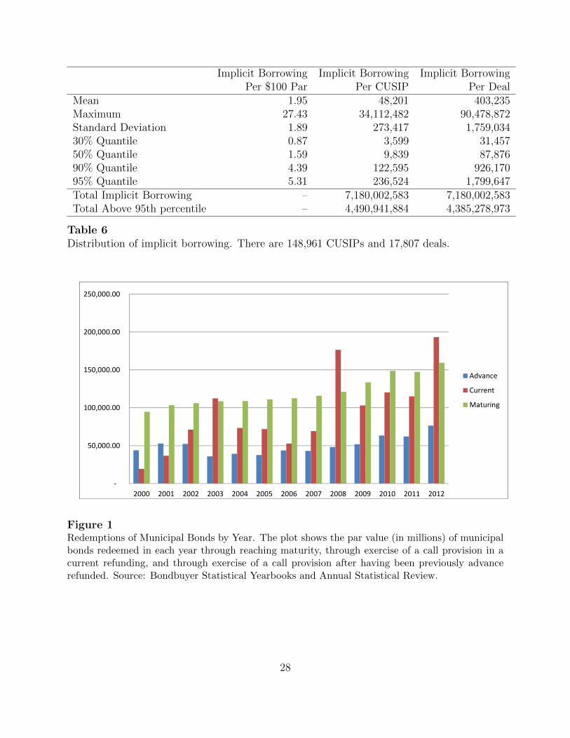
Implicit Borrowing Implicit Borrowing Implicit BorrowingPer $100 Par Per CUSIP Per Deal

Mean 1.95 48,201 403,235Maximum 27.43 34,112,482 90,478,872Standard Deviation 1.89 273,417 1,759,03430% Quantile 0.87 3,599 31,45750% Quantile 1.59 9,839 87,87690% Quantile 4.39 122,595 926,17095% Quantile 5.31 236,524 1,799,647Total Implicit Borrowing – 7,180,002,583 7,180,002,583Total Above 95th percentile – 4,490,941,884 4,385,278,973

Table 6Distribution of implicit borrowing. There are 148,961 CUSIPs and 17,807 deals.

 ‐

 50,000.00

 100,000.00

 150,000.00

 200,000.00

 250,000.00

2000 2001 2002 2003 2004 2005 2006 2007 2008 2009 2010 2011 2012

Advance

Current

Maturing

Figure 1Redemptions of Municipal Bonds by Year. The plot shows the par value (in millions) of municipalbonds redeemed in each year through reaching maturity, through exercise of a call provision in acurrent refunding, and through exercise of a call provision after having been previously advancerefunded. Source: Bondbuyer Statistical Yearbooks and Annual Statistical Review.

28

0

5000

10000

15000

20000

25000

30000

350000.5 1

1.5 2

2.5 3

3.5 4

4.5 5

5.5 6

6.5 7

7.5 8

8.5 9

9.5

10

10.5 11

11.5 12

12.5 13

13.5 14

14.5 15

15.5 16

16.5 17

17.5 18

18.5 19

19.5 20

20.5 21

21.5 22

22.5 23

23.5 24

24.5 25

Years to Call

Figure 2Years to Call Date for Pre-Refunded Municipal Bonds.

29

0

1000

2000

3000

4000

5000

6000

Number of Prerefundings

Month

Number of Prerefundings

0

2000

4000

6000

8000

10000

12000

14000

16000

18000

Par Value

Month

Par Value Prerefunded 

0.03

0.035

0.04

0.045

0.05

0.055

0.06

0.065

0.07

Av. 15 yr rate during month

Month

Long Muni Rate

Figure 3Volume of advance refundings by Month. The plot shows the number of pre-refundings, the parvalue (in millions) of pre-refundings, and the average 15-year zero-coupon tax-exempt yield for eachmonth during our sample period. The long municipal yield is from fitted zero-coupon yield curvescreated from MSRB transactions data.

30