Adjustment of positional geodetic networks by unconventional estimations

Acta Montanistica Slovaca Ročník 15 (2010), číslo 1, 71-85

71

Adjustment of positional geodetic networks by unconventional

estimations

Silvia Gašincová and Juraj Gašinec1

The content of this paper is the adjustment of positional geodetic networks by robust estimations. The techniques (based on the unconventional estimations) of repeated least-square method which have turned out to be suitable and applicable in the practise have been demonstrated on the example of the local geodetic network, which was founded to compose this thesis. In the thesis the following techniques have been chosen to compare the Method of least-squares with those many published in foreign literature: M-estimation of Biweight,M-estimation of Welsch and Danish method. All presented methods are based on the repeated least-square method principle with gradual changing of weight of individual measurements. In the first stage a standard least-square method was carried out in the following steps – iterations we gradually change individual weights according to the relevant instructions/ regulation (so-called weight function). Iteration process will be stopped when no deviated measurements are found in the file of measured data. MatLab programme version 5.2 T was used to implement mathematical adjustment.

Key words: Method of least squares, robust estimations, outlier detection

Introduction

In geodetic practice the method of least squares (hereafter in the text referred to as MNS) is generally used to analyze measured results. This method has several advantages – in case of normality of the sets of geodetic data measured it leads to the most reliable estimates of unknowns and provides statistically unbiased and consistent estimates of parameters. Due to the fact that not always all the conditions for its application are fulfilled, in the second half of the last century unconventional estimation techniques were developed in the theory of linear programming alongside standard estimation procedures. Of all these methods the so-called robust estimation techniques are mainly used in geodetic applications. These techniques allow obtaining estimates with various necessary properties and avoiding hidden, serious and systematic errors in measurements which could essentially effect and devalue the parameters being fixed. The known methods include e.g. the Method of the least sum of absolute values of corrections (hereafter in the text referred to as MNAS ) whose characteristic feature is robustness of the estimated parameters to the influence of outlying (deviating) measurements and the MINIMAX method (Cebecauer, D., 1994) that was applied mainly in the transformation of local networks. In foreign literature, especially in German and English (Jager et all, 2005) MNAS is defined as L1 standard.

The submitted paper compares the method of least squares with some types of robust methods based on the principle of its repetition (Weiss, et all, 2004),. Individual methods of adjustment are demonstrated on the local geodetic network which was established for the purpose of experimental measurement whilst preparing the thesis dissertation dealing with the issue of robust methods (Gašincová, S., 2007). The network situated in the locality of the Liptovská Mara water dam was measured by the combination of terrestrial and satellite measurements.

Adjustment of measurements

In geodesy the following processing procedures are used to evaluate the measured results (Böhm J.

et. al., 1990): a. adjustment of direct measurements where the only unknown was independently measured several times

(angle, length), b. adjustment of intermediate measurements where more unknowns were „determined“ by means of direct

measurement of other quantities which were in functional relationship with them, c. adjustment of conditional measurements where individual quantities are measured directly, but

at the same time d. they must fulfil a predetermined mathematical or geometrical condition

(e.g. in the triangle α+β+γ-200g = 0);

1 Silvia Gašincová, MSc, PhD., assoc. prof. Juraj Gašinec, MSc., PhD., Faculty of mining, ecology, procces control, and geotechnology,

Technical univerzity of Košice, Institute of Geodesy, Cartography and Geographic Information Systems, Park Komenského 19, 040 01 Košice, Slovak Republic, [email protected], [email protected]

(Review and revised version 31. 5. 2010)

Silvia Gašincová and Juraj Gašinec: Adjustment of positional geodetic networks by unconventional estimations

72

e. combined methods of adjustment: adjustment of intermediate measurements with conditions, adjustment of conditional measurements with the unknowns, collocation, the Kalman filter, the Chebyshev´s method, etc. The above-mentioned methods of adjustment are based on the condition of the minimum

of the correction vector norm. The norm is a number assigned to each n-dimensional vector vektoru )v...v,v(v n)n,( 211 = (Bitterer, 2006). The following types of the objective functions are most often used

in geodesy:

n1,i .minv)v(ppn

iii ∈=

⎟⎟

⎠

⎞

⎜⎜

⎝

⎛= ∑

=

1

1ρ (1)

Parameter p defines a special type of the objective function: a) for p=2 (L2-norma) the objective function has the following form

.minv)v(n

iii =⎟⎟

⎠

⎞⎜⎜⎝

⎛= ∑

=

21

1

2ρ , (2)

that leads to the method of least squares (MNS),

b) for p=1 (L1-norna) the objective function is expressed in the following form

.minv)v(n

iii == ∑

=1ρ , (3)

this represents the method of the least sum of absolute values of corrections (MNAS).

c) for p=∞ (L∞-norma) the objective function in the form

∞

=

∞⎟⎟⎠

⎞⎜⎜⎝

⎛= ∑

1

1

n

iii v)v(ρ , (4)

is changed into the MINIMAX method (known as the Chebyshev method) which minimizes the correction within a given tolerance interval (Bitterer, 2006) and for which applies that the biggest correction (its absolute value) is the minimum correction.

.minvmax i = (5) The methods of linear programming such as simplex method, its modified form Friedrich´s method

or solution in which the MNS is repeatedly used with gradual change of weights are applied when searching for the minimum by MINIMAX and MNAS methods.

Robust estimation techniques

There are, as we know, two types of robust estimation: robust estimation applied to MNS where the sum

of squares of corrections is replaced by more appropriate functions of corrections, e.g. the most reliable estimations (Huber, 1981; Hampel, 1986; etc.) and truly robust methods which include both the simplex and Friedrich´s method.

The robust method of adjustment based on the MNS principle takes place when in the estimation process the appropriately chosen correction function )v( iρ , the so-called loss (estimation) function is minimized (Sabová, Jakub, 2005).

min)v( i =ρ , (6)

that for the estimation process generates the so-called influence function )v( iΨ characterizing the influence of errors on the adjusted values for which applies


73

∑ =Ψ 0)( iv , (7) where

i

ii v

)v()v(∂

∂=

ρΨ . (8)

For the adjustment to be robust it is advisable to use iteration method with variable weights, so that

the weights of individual observations in each iteration step are determined as functions of corrections:

v)v()v(p i

iΨ

= , (9)

where )v(p i is a weight function in the solution of the adjustment method. Solution algorithm of the iteration robust estimation consists of the following steps : 1. in the first iteration step a standard MNS adjustment with weights 11

1 =)(p ((1)- iteration step for the ith observation) is performed, in case of heterogeneous measurements it is necessary to carry out their homogenization using P matrix (this function is available with MATLAB - rootm(P)) programme. An effective tool of solution without using P matrix in processing of heterogeneous measurements is given (Hemikogle, 2002),

2. from the corrections obtained in the first step of iteration using weight function )v(p i new weights are determined which will be used in the next step and analogically in the subsequent steps. Solution based on this principle represents an iteration solution with gradually changing weights pi

in accordance with the respective specification of observations so that with the sufficient number of iteration steps convergence of corrections takes place in the last steps.

Experimental measurement of the local geodetic network

Taking into consideration the fact that at present combining satellite and terrestrial measurements

creates a welcomed option of building, control and assessment of the quality of geodetic networks, the present paper presents a model of joint processing of satellite and terrestrial measurements (Leick, A, 1995).

The method of least squares and estimation techniques based on the principle of its repetition are demonstrated on the local geodetic network which was established for the purpose of developing the thesis on the site of the Liptovská Mara water dam. By choosing the site in the vicinity of the water dam we assumed formation of sufficient horizontal thermal gradient over the water surface and adjacent lands which would have a disturbing effect on terrestrial measurements (Bajtala, Sokol, 2005). For that reason, the measurement was carried out in the warm sunny environment. Unfortunately, the changed weather conditions during the measurement mixed up the heat blocks which is on the contrary a welcomed phenomenon in routine geodetic measurements

The geodetic network consists of four points (1,2,3,2643LM-1005) (fig. 1) which were temporarily stabilized by a steel rod of 12 mm diameter and 40 cm length – point 2643LM-1005 is a point of the State spatial network.

In terrestrial measurement, reflection prisms were placed at these points. Considering the fact that by combining GPS and terrestrial measurements it may lead to the situation when it is not possible to use the positions of GMS measurements for the terrestrial measurement due to the lack of direct visibility between the points, eccentric positions were stabilized in the vicinity of each of these standpoints the same way as points 1, 2, 3 from which the terrestrial measurement was carried out. Eccentric positions were marked according to the respective standpoints at 5001, 5002, 5003, 5005.

A single frequency GPS Stratus Sokkia system was used to carry out the satellite measurement which was performed by the static method simultaneously above all the network points (1, 2, 3, 1005). Four GPS devices were used in the measurement of the demonstration network. The approximate coordinates of the individual network points and their heights above the ellipsoid GRS80 in the coordinate system ETRS89 were determined from the point 2643LM-1005 (State spatial network) in the software package Spectrum Survey and Gues. From these coordinates, positional coordinates were determined in Gauss – Krüger projection.

Silvia Gaši

74

Fig. 1. Stru

Terrestriaof these of the geothe positThe sets s=12 grodirections(position

Fig. 2. Glo

Befo7 points ooptical raon adjustto the Zethe valueof the staplaced all

TakinecessarycoordinatSKPOS (ellipsoid

incová and Juraj

ucture of the posi

al measuremenpositions the

odetic networtions 5001, 5of directions oups were ms using the fo5002), LEICA

obal Positional Sy

ore the geodeon the campusangefinder aning conditioniss reflection

e of addition catic GPS metl at once in thing into consy to choose ates of the poi(Slovak spatiwhose param

Gašinec: Adjust

tional geodetic n

nt was performe sets of horizrk. With resp5003 and 500were measure

measured in nllowing instruA TCR 305 (po

ystem STRATUS

Proc

etic network s of the Technd mainly dete

nal adjustmenprisms for th

constant was sthod at the cee eccentric po

sideration the an appropriateints of the Staal observation

meters are ver

tment of position

etworks in the loc

med from the zontal directiect to the equ

05. In performed from indivn=4 directionsumental equiposition 5003)

Fig. 3.

Sokkia.

essing of the

measurementnical Universiermining an ants with unknhe devices of tset to c=-0,03entric points ositions 5001,5

mutual adjuse processing –ate spatial nen system) rel

ry close to W

nal geodetic netwo

cality of the Lipto

eccentric posons were meuipment used,

ming terrestriavidual eccentris. In position

pment: NIKONa LEICA TC

The time of obse

positional ge

t itself was pity for the pur

addition constnowns (Dobešthe Leica com

318 m. The gewith the terre5003,5003,50stment of the– computing

etwork as wellate to ETRS

WGS84 ellipso

orks by unconven

ovská Mara water

sitions 5001, 5easured in 12 , the slanted lal measuremeic positions. In 5002 s=11 N DTM 332 (p1800 (position

ervation on indiv

eodetic netwo

performed, therpose of verifant. The addi

š, J.,1990). Thmpany was c=eodetic networestrial measur05. satellite andspace before

ll as the coorS-89 coordinatoid (World G

froStandpoint [h:m

1 14:122 15:083 15:43

1005 16:15

ntional estimation

r dam.

5002, 5003 angroups to th

engths were ment 8 distancIn positions 50

groups wereposition 5001,n 5004).

vidual positions of

rk

ere was estabfying the funcition constant he addition c

=-0,0142 m, fork was measurements wher

d terrestrial me processing irdinates of thte system andeodetic Syste

om to timm:s] [h:m:s] 2:08 18:14:56 8:37 18:07:22 3:07 17:49:37 5:37 17:24:21

ns

nd 5005. Fromhe individual measured onlyces were mea001, 5003 ande measured in, KERN DKM

f the geodetic net

blished a basictionality of e

is calculatedconstant deterfor Nikon DTMured by combire the devices

measurements itself. Geograe reference sd GRS80 ref

em). Gauss co

me observation [h:m:s] 4:02:48 2:58:45 2:06:30 1:08:44

m each points

y from asured. d 5005 n n=4

M 2 – A

tworks.

is with electro-d based rmined M 352 ination s were

it was aphical tations

ference onform


75

projection of the ellipsoid in the meridian planes (also called Gauss-Kruger projection or Universal Transverse Mercator system – UTM ) or Lambert conform projection (Buchar, Hojovec, 1996; Daniš, 1976) are most often used for the direct projection of these coordinates to 2D computing space.

Because of this reason, during the period of network pre-processing the measured elements were

adjusted and subsequently reduced to the Gauss-Kruger projection chosen to be the computing space into which both satellite and terrestrial geodetic measurements were reduced and subsequently adjusted. In this projection as well as in its UTM modification in general both positive and negative plane coordinates x and y can occur which are called normal coordinates used for conversions between the neighbouring belts. Mainly negative y coordinates in each meridional belt appear to be a substantial disadvantage for our republic which is why the so-called conventional coordinates shifted 500 km to the west were introduced. In order to minimize the influence of longitudinal distortion and localization of all the points of the positional geodetic network in one meridional belt and in one coordinate system the Gauss Kruger projection is modified in such a way that the meridian belonging to the centre of the network is considered as a principal undistorted meridian. For that purpose the „ETRS 892Gauss.m” programme was written in Matlab programming language which rounded up the central meridian to full minutes. The conventional coordinates ( x – and y-coordinates shifted by a certain constant) are reduced in such a way that the value of x coordinate of the point 1 is 1000.000 m (tab. 2). For the direct display of geographical coordinates of the points on the geodetic network in the 2D computing space the following relations were used (Hojovec, 1987; Buchar, 1996; Pick, 1998).

( )

( )

( ) ( ) ( )( )( ) ( )( )ρλ∆ϕϕϕ

ρλ∆ϕϕρλ∆ϕ

ρλ∆ϕϕ

ϕϕρλ∆ϕϕ

ϕϕρλ∆ϕϕ

/sinecosettcos/N

/cosetcos/N/cosNY

/)sine/cosett

(cossin)/N()/)(cosecose

t(cossin)/N(/cossinN)/(SX

2222425

32223

222242

544422

232

5814185120

16

33027058

6172049

52421

′−′++−+

+′+−+=

′′++−

−+′+′+

+−++=

. (10)

Notes . S- the length of the meridian from the equator to the given geographical latitude ϕ , N- transverse radius of curvature , M- meridian radius of curvature , ϕ - geographical latitude of the converted point λ -geographical length of the converted point, e´-the second numerical eccentricity of the ellipsoid, t = tgϕ, ρ =57, 2957795° Tab. 1. Geographics coordinates points of the local geodetic network.

ϕ λ H point-[°]--[']-["]----[°]—[']—["] ---[m]----

1 49 5 31.40194 19 31 59.66451 604.580 2 49 5 55.84541 19 34 03.85359 607.692 3 49 6 33.10905 19 32 33.47193 603.9671005 49 6 15.38461 19 29 18.46236 608.5965001 49 5 31.49713 19 31 59.45874 603.9645002 49 5 56.02921 19 34 3.63487 606.8915003 49 6 33.14883 19 32 33.27692 604.3115005 49 6 15.28134 19 29 18.33564 607.969


76

Tab. 2. Coordinates in Gauss- Kruger projection. Normal coordinates Meridian Lenght influence lenght point x y h convergency distortion distortion

--------–––-[m]----------[m]--------[m]---------[°]-------------––––[cm/km]- 1 5439865.248 -6.806 604.580 -0.000070431 1.000000000 -0.00 2 5440620.929 2512.401 607.692 0.026003759 1.000000078 -0.01 3 5441771.55 678.845 603.967 0.007028720 1.000000006 -0.00 1005 5441224.96 -3276.473 608.596 -0.033918521 1.000000132 -0.01 5001 5439868.189 -10.981 603.964 -0.000113629 1.000000000 -0.00 5002 5440626.605 2507.961 606.891 0.025957858 1.000000077 -0.01 5003 5441772.783 674.890 604.311 0.006987771 1.000000006 -0.00 5005 5441221.747 -3279.046 607.969 -0.033945114 1.000000132 -0.01 Conventional coordinates 1 1000.000 4272.239 604.580 -0.000070431 1.000000000 -0.00 2 1755.680 6791.446 607.692 0.026003759 1.000000078 -0.01 3 2906.306 4957.891 603.967 0.007028720 1.000000006 -0.00 1005 2359.688 1002.572 608.596 -0.033918521 1.000000132 -0.01 5001 1002.941 4268.065 603.964 -0.000113629 1.000000000 -0.00 5002 1761.356 6787.007 606.891 0.025957858 1.000000077 -0.01 5003 2907.534 4953.936 604.311 0.006987771 1.000000006 -0.00 5005 2356.499 1000.000 607.969 -0.033945114 1.000000132 -0.01

Principle meridian: 19°32’ 0.00000” Distortion of the central meridian: 1.0000 Dx= -5438865.248 Dy= 4279.046 Note: All the coordinates of the network are located in one meridional belt according to the average geographical length.

For the transformation of the distances it is necessary to know the size of the longitudinal distortion in individual points of the network that are determined according to the relation:

(11)

In order to convert azimuth to bearings we need to know the size of the meridian convergence.

(12)

Taking into consideration the fact that the SSN (State spatial network) coordinates as well as

the coordinates of the SKPOS referential stations relate to the ETRS-89 coordinate system and GRS80 referential ellipsoid it was necessary to reduce individual parameters measured to the area of the mentioned ellipsoid before processing the geodetic network.

Distances measured terrestrially were also reduced into the plane of the cartographic projection. Before

the reduction itself distances measured were modified by an additive constant which was calculated with the help of conditional adjustment with the unknowns. The reduction of individual distances into the cartographic projection itself was performed in the following sequence: • calculation of the direct line connecting the endpoints of the distance measured, • calculation of the chord length in the substitute ball of the R radius, • the arc of a circle is calculated to the chord t , • recalculation of the arc of a circle to the length of the geodetic line on the reference ellipsoid.

As the geodetic network was measured from the eccentric standpoint it was necessary to convert

individual values obtained by terrestrial measurements to centric before the adjustment itself.

( ) ( )ϕϕληϕλ 244

222

45cos24

1cos2

1 tgm −+++=

( )

( )ϕϕϕρ

λ

ηηϕϕρλϕλγ

244

5

4222

3

2cossin15

231cossin3

sin

tg−+

++++=


77

The values determined in this way were the input data which were entered into the adjustment model (the vector of measured observations l) in the sequence of the terrestrial measurement - centric distances, centric angles a and GPS measurements – cartographic distances, pointers

Methods of development the issue

The method of least squares was used for mutual adjustment of the satellite and terrestrial measurements

which was compared with the following robust estimation procedures: 1. Danish method (Jäger, R. et al, 2005 ), 2. Robust M-estimate according to Biweight (Jäger, R.et al, 2005), 3. Robust M – estimate according to Welsch (Jäger, R.et al, 2005).

The above-mentioned estimation procedures are based on the principle of the repeated MLS. The geodetic network was adjusted as a free-network, i.e. all the coordinates of the geodetic network. 3 were adjusted. Before the network adjustment itself the homogeneity of precision of the measured quantities was tested. The testing was performed using an appropriate test to verify the homogeneity of variances of which Cochran statistics is used most frequently (Weiss, Sütti, 1997),(Weiss, et all, 2004), which was used in this case as well. Parameters of the 2nd order system were estimated by MINQUE (Minimum Norm Quadratic Unbiased Estimation) (Lucas, J. R. et all, 1998), separately for the satellite as well for terrestrial measurement for each device used.

Method of least squares Tab. 3. Free adjustment of LGN (Local geodetic network): Method of least squares. Measurement l l^ v pi Ti s(v) s(l^) r * f -----------------m ------ m --------- mm -----------------------*-- mm -------- mm -------------------- 1- 3 2025.8600 2025.8662 6.1539 0.0103 0.6294 9.6426 2.0158 0.958 79.5 1- 2 2630.0910 2630.1065 15.4909 0.0103 1.6651 9.6708 1.8760 0.964 81.0 3- 2 2164.6750 2164.6867 11.7218 0.0103 1.2272 9.6612 1.9249 0.962 80.5 3- 1 2025.8560 2025.8662 10.1539 0.0103 1.0558 9.6426 2.0158 0.958 79.5 3-1005 3992.9020 3992.9124 10.4153 0.0103 1.0805 9.6763 1.8473 0.965 81.2 1005- 3 3992.9110 3992.9124 1.4153 0.0103 0.1430 9.6763 1.8473 0.965 81.2 1005- 2 5820.3110 5820.3001 -10.8843 0.0103 1.1306 9.6876 1.7870 0.967 81.9 1005- 1 3541.1120 3541.1118 -0.1781 0.0103 0.0180 9.6636 1.9126 0.962 80.6 ----------------- g ------ g ---------- cc ------------------------- cc -------- cc --------------- 1-1005 0.0000 -0.0003 -2.7034 0.0658 0.8551 3.1420 2.3091 0.649 40.8 1- 3 96.8912 96.8914 1.8048 0.0658 0.5623 3.1593 2.2854 0.656 41.4 1- 2 156.3580 156.3581 0.8986 0.0658 0.2792 3.1496 2.2987 0.652 41.0 2- 1 0.0000 -0.0002 -2.3728 0.0658 0.7416 3.1665 2.2754 0.659 41.6 2-1005 25.1708 25.1711 2.8340 0.0658 0.8905 3.1675 2.2740 0.660 41.7 2- 3 54.2303 54.2303 -0.4612 0.0658 0.1426 3.1621 2.2815 0.658 41.5 3- 2 0.0000 -0.0001 -1.2940 0.0658 0.4046 3.1372 2.3157 0.647 40.6 3- 1 86.3025 86.3027 1.7007 0.0658 0.5298 3.1570 2.2886 0.656 41.3 3-1005 155.5796 155.5796 -0.4067 0.0658 0.1261 3.1510 2.2968 0.653 41.1 1005- 3 0.0000 0.0004 3.6644 0.0658 1.1624 3.1775 2.2600 0.664 42.0 1005- 2 15.3611 15.3615 4.0722 0.0658 1.3019 3.1769 2.2609 0.664 42.0 1005- 1 33.8326 33.8318 -7.7365 0.0658 2.7856 * 3.1755 2.2629 0.663 42.0 -------------- m ------ m ---------- mm ---------------------------- mm -------- mm -------------------1005- 2 5820.3030 5820.3001 -2.8843 0.1524 1.6300 1.8350 1.7870 0.653 30.2 1005- 3 3992.9110 3992.9124 1.4153 0.1524 0.7909 1.7742 1.8473 0.664 27.9 1-1005 3541.1100 3541.1118 1.8219 0.1524 1.0730 1.7037 1.9126 0.664 25.3 1- 2 2630.1060 2630.1065 0.4909 0.1524 0.2755 1.7439 1.8760 0.663 26.8 1- 3 2025.8680 2025.8662 -1.8461 0.1524 1.1785 1.5803 2.0158 0.513 21.3 2- 3 2164.6860 2164.6867 0.7218 0.1524 0.4190 1.6898 1.9249 0.480 24.8 -------------- g ------ g ---------- cc ---------------------------- cc -------- cc -------------------1005- 2 106.6186 106.6185 -0.9969 1.0913 1.1735 0.8567 0.4270 0.801 55.4 1005- 3 91.2574 91.2574 -0.4047 1.0913 0.5099 0.7802 0.5546 0.664 42.1 1-1005 325.0887 325.0888 1.1945 1.0913 1.6748 0.7419 0.6049 0.601 36.8 1- 2 81.4471 81.4472 0.7964 1.0913 1.0885 0.7348 0.6135 0.589 35.9 1- 3 21.9805 21.9805 -0.2973 1.0913 0.4092 0.7128 0.6390 0.554 33.2 2- 3 335.6777 335.6777 -0.2920 1.0913 0.4266 0.6717 0.6820 0.492 28.8

v* - Outlier detection Ti ~ t(alfa,f-1) = 2.080 r* - Measurement uncontrollable for the presence of a gross error (r*<0.30) 2nd order PARAMETERS Standard deviation of the bases measured electronically: 9.85 mm Standard deviation of measured directions: 3.90 cc Standard deviation of measured GPS bases: 2.56 mm Standard deviation of measured GPS pointers: 0.96 cc


78

Tab. 4. Coordinates. X° Y° dX^ dY^ dC^ X^ Y^ sX^ sY^ sxy sp ----- [m] ------ [m] ----- [mm] ----[mm] ---- [mm] -*--- [m] -------- [m] ----- [mm] -- [mm]-- [mm] -- [mm] 1 1000.000 4272.239 -0.8412 -0.4074 0.9346 999.9992 4272.2386 1.4435 1.1988 1.33 1.88 2 1755.680 6791.446 -0.3081 0.2231 0.3804 1755.6797 6791.4462 1.8365 1.1107 1.52 2.15 3 2906.306 4957.891 2.0926 0.5098 2.1538 2906.3081 4957.8915 1.4495 1.1566 1.31 1.85 1005 2359.688 1002.572 -0.9433 -0.3255 0.9979 2359.6871 1002.5717 2.4965 1.1133 1.93 2.73

Points exceeding the limit of linearization Significance level alpha chosen* = 0.050 Number of critical measurements* = 1 Standard deviation a priori = 1.000 Critical limit s0_a posterior = 1.242 s0_aposter^2/s0_aprior^2 = 1.000 Crit. ratio s0_aposter^2/s0_aprior^2 = 1.542 Average side length [m] = 3274.215 Average coordinate error in the network [mm] = 1.543 Average positional error in the network [mm] = 2.182 Effectiveness of adjustment = 0.786 Redundancy = 22.000 tr(R) = 22.000 Critical values of the distribution functions t(Alfa,f) = 2.074 chi^2(Alfa,f) = 33.924 Decrease of the rank of the configuration matrix = 2

Tab. 5. Error ellipses.

Standard error ellipses Confidence errors of ellipses For the probability 95.0 percent

point a b convolution(a) a b convolution(a) -------- [mm] ------- [mm] ----- [g] ----- ------- [mm] ------- [mm] ----- [g] -----

1 1.448 1.193 9.0190 3.800 3.131 9.0190 2 1.839 1.106 4.5280 4.827 2.902 4.5280 3 1.456 1.148 389.9889 3.822 3.013 389.9889 1005 2.508 1.088 6.7189 6.581 2.854 6.7189

Tab. 6. Free adjustment of the LGN: MLS after introducing the change of scale.

Terresstrial measurements

Measurement l l^ v pi Ti s(v) s(l^) r * f --------- m -----–- m ------- mm ----------------------- mm ------ mm -----------------

1- 3 2025.8600 2025.8645 4.5478 0.0100 0.4637 9.6230 2.7653 0.924 72.4 1- 2 2630.0910 2630.1043 13.2855 0.0100 1.4347 9.4907 3.1898 0.899 68.1 3- 2 2164.6750 2164.6849 9.8516 0.0100 1.0296 9.5824 2.9027 0.916 71.0 3- 1 2025.8560 2025.8645 8.5478 0.0100 0.8836 9.6230 2.7653 0.924 72.4 3-1005 3992.9020 3992.9091 7.1017 0.0100 0.7750 9.0758 4.2282 0.822 57.8 1005- 3 3992.9110 3992.9091 -1.8983 0.0100 0.2043 9.0758 4.2282 0.822 57.8 1005- 2 5820.3110 5820.2952 -15.8395 0.0100 2.1328 * 8.0298 5.9808 0.643 40.3 1005- 1 3541.1120 3541.1088 -3.2146 0.0100 0.3421 9.1981 3.9553 0.844 60.5 -------------- g ------ g ------ cc ------------------------ cc ------ cc ----------------- 1-1005 0.0000 -0.0003 -2.7071 0.0657 0.8559 3.1428 2.3098 0.649 40.8 1- 3 96.8912 96.8914 1.8187 0.0657 0.5661 3.1603 2.2858 0.657 41.4 1- 2 156.3580 156.3581 0.8884 0.0657 0.2757 3.1505 2.2992 0.652 41.0 2- 1 0.0000 -0.0002 -2.3838 0.0657 0.7446 3.1674 2.2759 0.660 41.6 2-1005 25.1708 25.1711 2.8246 0.0657 0.8870 3.1683 2.2747 0.660 41.7 2- 3 54.2303 54.2303 -0.4408 0.0657 0.1361 3.1630 2.2820 0.658 41.5 3- 2 0.0000 -0.0001 -1.2785 0.0657 0.3992 3.1380 2.3163 0.647 40.6 3- 1 86.3025 86.3027 1.7089 0.0657 0.5318 3.1580 2.2890 0.656 41.3 3-1005 155.5796 155.5796 -0.4304 0.0657 0.1333 3.1517 2.2976 0.653 41.1 1005- 3 0.0000 0.0004 3.6564 0.0657 1.1598 3.1784 2.2605 0.664 42.0 1005- 2 15.3611 15.3615 4.0737 0.0657 1.3031 3.1777 2.2615 0.664 42.0 1005- 1 33.8326 33.8318 -7.7301 0.0657 2.8029 * 3.1764 2.2634 0.663 42.0

GPS measurements

-------------- m ------ m ------- mm ------------------------ mm ------ mm ----------------- 1005- 2 5820.3030 5820.3005 -2.5089 0.1559 1.4629 1.7610 1.8202 0.653 28.1 1005- 3 3992.9110 3992.9128 1.7586 0.1559 1.0377 1.6979 1.8791 0.664 25.8 1-1005 3541.1100 3541.1120 2.0286 0.1559 1.2429 1.6532 1.9186 0.664 24.2 1- 2 2630.1060 2630.1067 0.6943 0.1559 0.3991 1.7048 1.8729 0.663 26.0 1- 3 2025.8680 2025.8664 -1.5968 0.1559 1.0471 1.5285 2.0193 0.483 20.3 2- 3 2164.6860 2164.6868 0.8341 0.1559 0.4944 1.6565 1.9157 0.449 24.4 ------------g ------ g ------- cc ------------------------ cc ------ cc ----------------- 1005- 2 106.6186 106.6185 -1.0045 1.0755 1.1738 0.8634 0.4296 0.802 55.5 1005- 3 91.2574 91.2574 -0.4218 1.0755 0.5265 0.7872 0.5570 0.666 42.2 1-1005 325.0887 325.0888 1.1917 1.0755 1.6551 0.7492 0.6072 0.604 37.0 1- 2 81.4471 81.4472 0.7871 1.0755 1.0631 0.7427 0.6152 0.593 36.2 1- 3 21.9805 21.9805 -0.2826 1.0755 0.3835 0.7216 0.6397 0.560 33.7 2- 3 335.6777 335.6777 -0.2699 1.0755 0.3891 0.6796 0.6842 0.497 29.1


79

Change of scale for electro-optical rangefinders = 1.00000092 v* - Outlier detection; Ti ~ t(alfa,f-1) = 2.086 r* - Measurement uncontrollable for the presence of a gross error (r*<0.30)

The method of least squares found two outlier detections in measuring the direction from the standpoint 1005-1 and the distance from the standpoint 1005-2. After the adjustment of the network by this method we came to the conclusion that corrections in the terrestrially measured bases indicate a systematic trend the cause of which can be attributed to the insufficient introduction of the physical corrections taking into account the size of the network. Because of this reason the change of scale was also estimated in electro-optical rangefinders (Nevosád, Z. at al, 2002). 2nd order PARAMETERS ----------------–––– Standard deviation of the bases measured electronically: 10.01 mm Standard deviation of measured directions : 3.90 cc Standard deviation of measured GPS bases : 2.53 mm Standard deviation of measured GPS pointers : 0.96 cc

Tab. 7 Coordinates. X° Y° dX^ dY^ dC^ X^ Y^ sX^ sY^ sxy sp -----[m]----- [m] ----- [mm] ---[mm] ---[mm] -*- -[m] ------ [m] -----[mm] -- [mm]---[mm]--[mm]

1 1000.000 4272.239 -0.9359 -0.4363 1.0326 999.9991 4272.2386 1.4446 1.1958 1.33 1.88 2 1755.680 6791.446 -0.3076 0.3780 0.4874 1755.6797 6791.4464 1.8455 1.1132 1.52 2.16 3 2906.306 4957.891 2.2165 0.6095 2.2988 2906.3082 4957.8916 1.4537 1.1598 1.31 1.86 1005 2359.688 1002.572 -0.9730 -0.5512 1.1183 2359.6870 1002.5714 2.5097 1.1361 1.95 2.75


Standard error ellipses Confidence errors of ellipses For the probability 95.0 percent

point a b convolution(a) a b convolution(a) -------- [mm] ---- [mm] ----- [g] ----- ------- [mm] ---- [mm] ----- [g] --- 1 1.449 1.191 8.6914 3.815 3.135 8.6914 2 1.849 1.108 4.6732 4.868 2.917 4.6732 3 1.459 1.153 390.8976 3.842 3.035 390.8976 1005 2.522 1.109 6.9268 6.640 2.921 6.9268

As it is obvious from the output of the solution there was a positive adjustment of corrections

in the distances measured electro-optically. Introducing the change of scale into the adjustment resulted in a better conditionality of the criteria matrix S where the number of conditionality cond(S) decreased from 4,828.103 to 2,853.103 and subsequently faster convergence of the variance components (average errors) of the devices used. The MLS revealed two outlier detections. In the case where the method reveals deviating measurements the standard procedure includes exclusion of such measurements from the file of the measured data.

Fig.4. Absolute confidence error ellipses - Method of least squares.

ABSOLUTE CONFIDENCE ERROR ELLIPSES α=0,05 %

ellipses with outulier measured ellipses after out otulier measured

KEY:


80

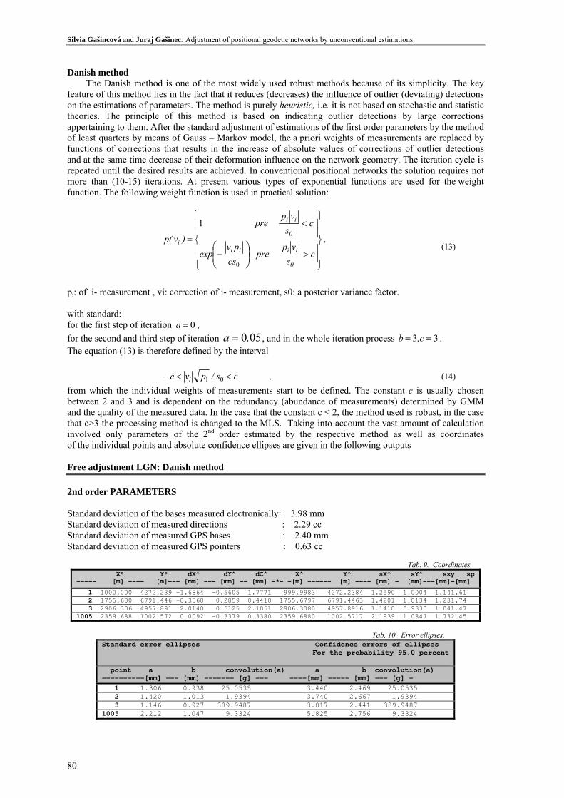
Danish method The Danish method is one of the most widely used robust methods because of its simplicity. The key

feature of this method lies in the fact that it reduces (decreases) the influence of outlier (deviating) detections on the estimations of parameters. The method is purely heuristic, i.e. it is not based on stochastic and statistic theories. The principle of this method is based on indicating outlier detections by large corrections appertaining to them. After the standard adjustment of estimations of the first order parameters by the method of least quarters by means of Gauss – Markov model, the a priori weights of measurements are replaced by functions of corrections that results in the increase of absolute values of corrections of outlier detections and at the same time decrease of their deformation influence on the network geometry. The iteration cycle is repeated until the desired results are achieved. In conventional positional networks the solution requires not more than (10-15) iterations. At present various types of exponential functions are used for the weight function. The following weight function is used in practical solution:

, c

svp

pre cs

pvexp

cs

vp pre

)v(p

0

iiii

0

ii

i

⎪⎪

⎭

⎪⎪

⎬

⎫

⎪⎪

⎩

⎪⎪

⎨

⎧

>⎟⎟⎠

⎞⎜⎜⎝

⎛−

<

=

0

1

(13)

pi: of i- measurement , vi: correction of i- measurement, s0: a posterior variance factor. with standard: for the first step of iteration 0=a , for the second and third step of iteration 050.a = , and in the whole iteration process 33 == c,b . The equation (13) is therefore defined by the interval

cs/pv c i <<− 01 , (14)

from which the individual weights of measurements start to be defined. The constant c is usually chosen between 2 and 3 and is dependent on the redundancy (abundance of measurements) determined by GMM and the quality of the measured data. In the case that the constant c < 2, the method used is robust, in the case that c>3 the processing method is changed to the MLS. Taking into account the vast amount of calculation involved only parameters of the 2nd order estimated by the respective method as well as coordinates of the individual points and absolute confidence ellipses are given in the following outputs Free adjustment LGN: Danish method 2nd order PARAMETERS Standard deviation of the bases measured electronically: 3.98 mm Standard deviation of measured directions : 2.29 cc Standard deviation of measured GPS bases : 2.40 mm Standard deviation of measured GPS pointers : 0.63 cc

Tab. 9. Coordinates. X° Y° dX^ dY^ dC^ X^ Y^ sX^ sY^ sxy sp –---- [m] –--- [m]–-- [mm] –-- [mm] –- [mm] -*– -[m] –----- [m] –--- [mm] – [mm]–--[mm]–[mm]

1 1000.000 4272.239 -1.6864 -0.5605 1.7771 999.9983 4272.2384 1.2590 1.0004 1.141.61 2 1755.680 6791.446 -0.3368 0.2859 0.4418 1755.6797 6791.4463 1.4201 1.0134 1.231.74 3 2906.306 4957.891 2.0140 0.6125 2.1051 2906.3080 4957.8916 1.1410 0.9330 1.041.47 1005 2359.688 1002.572 0.0092 -0.3379 0.3380 2359.6880 1002.5717 2.1939 1.0847 1.732.45


Standard error ellipses Confidence errors of ellipses For the probability 95.0 percent point a b convolution(a) a b convolution(a) ––---––––-[mm] ––- [mm] ––––––- [g] ––- ––––[mm] ––––- [mm] ––- [g] – 1 1.306 0.938 25.0535 3.440 2.469 25.0535 2 1.420 1.013 1.9394 3.740 2.667 1.9394 3 1.146 0.927 389.9487 3.017 2.441 389.9487 1005 2.212 1.047 9.3324 5.825 2.756 9.3324


81

Fig. 5. Absolute confidence error ellipses - Danish method.

In adjustment the particular geodetic network, the relationship 13 defined by the interval 14 dependent

on the so-called damping constant c which is chosen by the designer was used for calculation of individual weights. After the network adjustment in the first cycle two deviating measurements (length 1005-2 and direction 1005-1) were also detected. In further cycles the weights of measurements began to decrease. Iteration process stopped in the fifth cycle at the damping constant c=1.57. Robust M- estimation according to Biweight For this estimation the following constants are used: weighting function

⎪⎪⎭

⎪⎪⎬

⎫

⎪⎪⎩

⎪⎪⎨

⎧

>

≤⎟⎟

⎠

⎞

⎜⎜

⎝

⎛⎟⎠⎞

⎜⎝⎛−

=

av

av av

)v(p

0

122

Fig. 6. Graphical course weighting function. Free adjustment LGN: M – estimation according to Biweight 2nd order PARAMETERS ––------------- Standard deviation of the bases measured electronically: 3.19 mm Standard deviation of measured directions : 1.71 cc Standard deviation of measured GPS bases : 2.03 mm Standard deviation of measured GPS pointers : 0.62 cc

Tab. 11. Coordinates. X° Y° dX^ dY^ dC^ X^ Y^ sX^ sY^ sxy sp –––––[m] –––––––-[m] ––––-[mm] –––[mm] – [mm] -*––– [m]––-–– [m]––---–-[mm] –––[mm]––-[mm]––-[mm]

1 1000.000 4272.239 -1.3854 -0.4544 1.4580 999.9986 4272.2385 1.2097 0.9443 1.09 1.5 2 1755.680 6791.446 -0.6736 0.2044 0.7039 1755.6793 6791.4462 1.4749 0.9722 1.25 1.7 3 2906.306 4957.891 2.0423 0.4016 2.0814 2906.3080 4957.8914 1.0922 0.8860 0.99 1.4 1005 2359.688 1002.572 0.0167 -0.1516 0.1525 2359.6880 1002.5718 2.1675 1.0904 1.72 2.4


00,20,40,60,8

1

-8 -6 -4 -2 0 2 4 6 8

p(v)

v

Graphical course weighting function


82

Tab. 12. Error ellipses. Standard error ellipses Confidence errors of ellipses For the probability 95.0 percent point a b convolution(a) a b convolution(a) –----- [mm] –----–––-[mm] –--- [g] –--- –----––––[mm] –----–- [mm] –--- [g] –--- 1 1.230 0.918 17.4338 3.238 2.417 17.4338 2 1.475 0.972 0.0681 3.884 2.560 0.0681 3 1.098 0.879 388.8753 2.892 2.314 388.8753 005 2.182 1.061 8.4690 5.746 2.793 8.4690

Fig. 7. Aabsolute confidence error ellipses- Biweight.

This method stopped in the fourth iteration cycle using the damping constant c=4.685. Robust M-estimation according to Welsch Weighting function: ( )2a/ve)v(p −= Fig. 8. Graphical course weighting function. Free adjustment LGN: M – estimation according to Welsch 2nd order PARAMETERS Standard deviation of the bases measured electronically: 3.12 mm Standard deviation of measured directions : 1.70 cc Standard deviation of measured GPS bases : 1.95 mm Standard deviation of measured GPS pointers : 0.58 cc

Tab. 13. Coordinates X° Y° dX^ dY^ dC^ X^ Y^ sX^ sY^ sxy sp ------[m] ----- [m] ---- [mm] -- [mm] - [mm] -*---[m]-------[m]-- --[mm]---[mm]--[mm]--[mm]- 1 1000.000 4272.239 -1.4353 -0.5024 1.5207 999.9986 4272.2385 1.1982 0.9173 1.07 1.51 2 1755.680 6791.446 -0.6779 0.1320 0.6906 1755.6793 6791.4461 1.4276 0.9520 1.21 1.72 3 2906.306 4957.891 2.0245 0.4853 2.0818 2906.3080 4957.8915 1.0614 0.8578 0.96 1.36 1005 2359.688 1002.572 0.0887 -0.1148 0.1451 2359.6881 1002.5719 2.1219 1.0867 1.69 2.38 * Points exceeding the points of linearization

00,20,40,60,8

11,2

-6 -4 -2 0 2 4 6

p(v)

v

Graphical course weighting function



83

Tab. 14. Error ellipses. Standard error ellipses Confidence errors of ellipses For the probability 95.0 percent point a b convolution(a) a b convolution(a) -------- [mm] ------- [mm] ----- [g] ----- ------- [mm] ------- [mm] ----- [g] ----- 1 1.217 0.892 16.6105 3.205 2.349 16.6105 2 1.428 0.952 399.2342 3.759 2.507 399.2342 3 1.066 0.852 390.3326 2.806 2.244 390.3326 1005 2.137 1.057 8.6604 5.627 2.784 8.6604

Fig. 9. The absolute confidence error ellipses – Welsch.

Tab. 15. Results of adjustment. Measurand v pi v pi v pi v pi --------- -- mm --------- -- mm ---------- -- mm ---------- ----mm -------- 1- 3 4.5478 0.0100 5.8820 0.0023 5.3933 0.0147 5.5169 0.0130 1- 2 13.2855 0.0100 14.5303 0.0000 14.0052 0.0000 14.0584 0.0000 3- 2 9.8516 0.0100 10.5074 0.0001 10.6777 0.0000 10.5905 0.0000 T 3- 1 8.5478 0.0100 9.8820 0.0001 9.3933 0.0000 9.5169 0.0001 E 3-1005 7.1017 0.0100 8.2596 0.0022 7.6230 0.0115 7.7535 0.0108 R 1005- 3 -1.8983 0.0100 -0.7404 0.0632 -1.3770 0.0890 -1.2465 0.0903 R 1005- 2 -15.8395 0.0100 -13.8105 0.0003 -14.3997 0.0007 -14.3600 0.0007 E 1005- 1 -3.2146 0.0100 -1.5056 0.0632 -1.9104 0.0694 -1.8565 0.0666 S -------- - cc ---------- --cc ------------ cc ---------- --- cc -------- T 1-1005 -2.7071 0.0657 D -2.4379 0.1901 B -2.6903 0.1378 W -2.7118 0.1196 R 1- 3 1.8187 0.0657 A 1.7563 0.1901 I 1.4824 0.2309 E 1.4703 0.2152 I 1- 2 0.8884 0.0657 N 0.6816 0.1901 W 0.6072 0.3141 L 0.5474 0.3100 A 2- 1 -2.3838 0.0657 I -2.5222 0.1901 E -2.3108 0.1680 S -2.3069 0.1495 L 2-1005 2.8246 0.0657 S 2.9647 0.1901 I 3.0818 0.1185 C 3.1075 0.1024 2- 3 M -0.4408 0.0657 H -0.4425 0.1901 G -0.2952 0.3357 H -0.2580 0.3358 3- 2 L -1.2785 0.0657 -1.3513 0.1901 H -1.2351 0.2808 -1.2285 0.2717 3- 1 S 1.7089 0.0657 M 1.6437 0.1901 T 1.6245 0.2379 1.6455 0.2231 3-1005 -0.4304 0.0657 E -0.2924 0.1901 -0.2588 0.3370 -0.2581 0.3366 1005- 3 3.6564 0.0657 T 1.4123 0.0075 -0.0385 0.0933 0.1176 0.0743 1005- 2 4.0737 0.0657 H 1.7606 0.0052 0.3623 0.0651 0.5127 0.0502 1005- 1 -7.7301 0.0657 O -9.8458 0.0002 -11.3278 0.0000 -11.1609 0.0000 -------- -- mm --------- D -- mm -------- -- mm ---------- -- mm --------- 1 005- 2 -2.5089 0.1559 -2.7077 0.1733 -2.9384 0.0778 -3.0390 0.0696 1005- 3 1.7586 0.1559 1.3882 0.1733 0.9976 0.1540 1.0318 0.1494 G 1-1005 2.0286 0.1559 2.3822 0.1733 2.1955 0.1293 2.1640 0.1225 P 1- 2 0.6943 0.1559 0.9324 0.1733 0.5694 0.2208 0.5591 0.2361 S 1- 3 -1.5968 0.1559 -1.0380 0.1733 -1.4019 0.1693 -1.3272 0.1706 2- 3 0.8341 0.1559 0.6614 0.1733 0.9650 0.2137 0.8256 0.2278 -------- - cc --------- -- cc -------- --- cc -------- -- cc -------- 1005- 2 -1.0045 1.0755 -0.8910 0.0237 -0.8505 0.0885 -0.8409 0.0744 1005- 3 -0.4218 1.0755 -0.2393 2.4856 -0.2513 1.9269 -0.2361 2.0265 1-1005 1.1917 1.0755 1.5026 0.0494 1.4594 0.2340 1.4855 0.1980 1- 2 0.7871 1.0755 0.6221 2.4856 0.7569 1.0105 0.7447 0.9572 1- 3 -0.2826 1.0755 -0.3032 2.4856 -0.3679 2.3301 -0.3324 2.5631 2- 3 -0.2699 1.0755 -0.2982 2.4856 -0.2275 2.3742 -0.2065 2.6334



84

The above-mentioned method found two outlier detections in the first cycle and stopped in the fourth iteration cycle. Table 19 gives the results of the adjustment directions measured terrestrially, electro-optically measured lengths and GPS vectors reduced to bases and pointers in the positional computational space in the cartographic plane. Tab. 16. 2nd order parameters estimated by individual methods.

MLS Danish BIWEIGHT WELSCH Standard deviation of the bases measured electronically [mm] 10.01 3.98 3.19 3.12 Standard deviation of measured directions [cc] 3.90 2.29 1.71 1.70 Standard deviation of measured GPS bases [mm] 2.53 2.40 2.03 1.95 Standard deviation of measured GPS pointers [cc] 0.96 0.63 0.62 0.58

Tab. 17. Adjustment coordinates complemets.

MLS Danish BIWEIGHT WELSCH

dC^[mm] dC^[mm] dC^[mm] dC^[mm] 1 1.0326 1.7771 1.4580 1.5207 2 0.4874 0.4418 0.7039 0.6906 3 2.2988 2.1051 2.0814 2.0818

1005 1.1183 0.3380 0.1525 0.1451

Conclusion

The objective of the submitted paper is to compare the method of least squares with some types

of robust estimation procedures. The following procedures: M-estimation according to Biweight, M-estimation according to Welsch and the Danish method were chosen from a number of estimation procedures published in the foreign literature and compared with the MLS MatLab programme version 5.2 T was used to implement the mathematical adjustment. Table 15 shows the conformity of the individual tested robust estimation methods and their effect on the corrections with respect to the MLS. Based on the results obtained in the processing of this experimental geodetic network it seems reasonable to suggest that the adjustment methods used produce comparable results shown not only in the above-mentioned Table but also in the similar graphic course of the functions of individual estimation procedures. All the methods stopped after the fourth iteration cycle whereas the biggest corrections took place in the measurements of directions from the standpoint 1005-1 and measurement of the length from the standpoint 1005-2.

In spite of the fact that the standard method used in geodetic surveying is the MLS it is necessary to pay sufficient attention also to alternative estimation methods. The current significance of the topic is supported by the fact that the use of unconventional estimation procedures in the recent years has been more and more often discussed also in foreign literature (Jager et all, 2005). These methods are applicable mainly in the cases where it is not possible to influence the intersection of outlying-deviating measurements to the file of measured data. Though in the paper these methods are presented only on the positional geodetic network, they can be applied in other fields of geodetic survey such as deformation survey.

Tento článok bol vytvorený realizáciou projektu Centrum excelentného výskumu získavania a spracovania zemských zdrojov, na základe podpory operačného programu Výskum a vývoj financovaného z Európskeho fondu regionálneho rozvoja a grantového projektu číslo 1/0786/10 Vedeckej grantovej agentúry MŠ SR Výskum dynamiky ľadovej výplne jaskynných priestorov bezkontaktnými metódami z hľadiska ich bezpečného a trvalo udržateľného využívania ako súčasti prírodného dedičstva Slovenskej republiky.

References

[1] Bajtala, M., Sokol, Š: Odhad variančných komponentov z meraní v geodetickej sieti. Acta Montanistica Slovaca, roč.2, č. 10, s. 68-77, Košice, 2005.

[2] Bitterer, L.: Vyrovnávací počet. Žilinská univerzita, Žilina, 2006. [3] Böhm, J., Radouch, V., Hampacher, M.: Teorie chyb a vyrovnávací počet, Praha, Geodetický

a kartografický podnik, 1990.


85

[4] Buchar, P, Hojovec, V.: Matematická kartografie 10, ČVUT, Praha, 1996. [5] Cebecauer, D.: Kombinované použitie metód najmenších štvorcov, najmenšej sumy absolútnych

hodnôt opráv a MINIMAX, Geodetický a kartografický obzor, 40 (82), 1994 č.11, s. 221-225. [6] Daniš, M.: Matematická kartografia, Stavebná fakulta, Bratislava, 1976. [7] Dobeš, J. a kol.: Presné lokálne geodetické siete, Výskumný ústav geodézie a kartografie, Bratislava

1990. [8] Gašincová, S.: Spracovanie 2D sietí pomocou robustných metód. Doktorandská dizertačná práca.

Košice 2007, str.91. [9] Hampel, F. et al: Robust statistics, the approach based of influence functions. J.Willey&Sons, New

York, 1986. [10] Hojovec, V.: Kartografie, Geodetický a kartografický podnik, Praha, 1987. [11] Huber, P. J.: Robust estimation of a location parameter. Ann Math Stat 35: 73-101, 1964. [12] Hekimoglu, S., Berber, M.: Effectiveness of robust methods in heterogeneous linear models., Journal

of Geodesy, 76, 706-713, 2003. [13] Jäger, R., Műlle, T., Saler, H. Schväble, R.: Klassischle und robuste Ausgleichungsverfahren, Herbert

Wichmann Verlag, Heidelberg, 2005. [14] Leick, A.: GPS satellite surveying. John Wiley & Sons, 560 s ,1995. [15] Lucas, J.R., Dillinger, W. H.: MINQUE for block diagona bordered systems such as those encuntered

in VLBI data analysis. Journal of Geodesy, 72, 343-349, 1998. [16] Pick, M.: Geodézie. Súradnicové systémy a zobrazení, STU, Bratislava, 1998. [17] Nevosád, Z.,Vitásek, J., Bureš, J.: Geodézie IV. Souřadnicové výpočty, CERM, s.r.o Brno, 2002. [18] Sabová, J., Jakub, V. Geodetické deformačné šetrenie. ES/AMS, Fakulta BERG TU v Košiciach,

ISBN 978-80-8073-788-7, Košice, 2007. [19] Weiss, G., Sűtti, J.: Geodetické lokálne siete I, Košice 1997. [20] Weiss,G., Labant, S., Weiss, E., Mixtaj, L., Schwarczová, H.: Establishment of Local Geodetic Nets.

Acta Montanistica Slovaca, Ročník 14 (2009), číslo 4, 306-313, ISSN 1335-1778. [21] Weiss G., Jakub, V., Weiss. E.: Kompatibilita geodetických bodov a jej overovanie. TU Košice, 2004,

ISBN: 80-8073-149-7.

Adjustment of positional geodetic networks by unconventional estimations

Documents

Transcript of Adjustment of positional geodetic networks by unconventional estimations