Addressing Industrial Waste Heat Supply VariabilityWith Organic Rankine Cycle Systems IncorporatingThermal Energy StorageBipul Krishna Saha 

Indian Institute of Technology KharagpurBasab Chakraborty  ( basab@see.iitkgp.ernet.in )

Indian Institute of Technology, Kharagpur https://orcid.org/0000-0002-8444-7402Rohan Dutta 

Indian Institute of Technology Kharagpur

Research Article

Keywords: Low- grade waste heat, Power generation, Organic Rankine Cycle, Working �uids, Thermo-economic analysis, Aspen Hysys®

Posted Date: July 7th, 2021

DOI: https://doi.org/10.21203/rs.3.rs-658624/v1

License: This work is licensed under a Creative Commons Attribution 4.0 International License.  Read Full License

1

Addressing industrial waste heat supply variability with organic Rankine cycle systems incorporating thermal energy storage

Bipul Krishna Saha1, Basab Chakraborty1, Rohan Dutta2

1Rajendra Mishra School of Engineering Entrepreneurship, Indian Institute of Technology, Kharagpur, Paschim Medinipur, West Bengal, India-721302

2Cryogenic Engineering Centre, Indian Institute of Technology, Kharagpur, Paschim Medinipur, West Bengal, India-721302

Abstract

Industrial low-grade waste heat is lost, wasted and deposited in the atmosphere and is not put to any

practical use. Different technologies are available to enable waste heat recovery, which can enhance

system energy efficiency and reduce total energy consumption. Power plants are energy-intensive plants

with low-grade waste heat. In the case of such plants, recovery of low-grade waste heat is gaining

considerable interest. However, in such plants, power generation often varies based on market demand.

Such variations may adversely influence any recovery system's performance and the economy,

including the Organic Rankine Cycle (ORC). ORC technologies coupled with Cryogenic Energy

Storage (CES) may be used for power generation by utilizing the waste heat from such power plants.

The heat of compression in a CES may be stored in thermal energy storage systems and utilized in ORC

or Regenerative ORC (RORC) for power generation during the system's discharge cycle. This may

compensate for the variation of the waste heat from the power plant, and thereby, the ORC system may

always work under-designed capacity. This paper presents the thermo-economic analysis of such an

ORC system. In the analysis, a steady-state simulation of the ORC system has been developed in a

commercial process simulator after validating the results with experimental data for a typical coke-oven

plant. Forty-nine different working fluids were evaluated for power generation parameters, first law

efficiencies, purchase equipment cost, and fixed investment payback period to identify the best working

fluid.

Keywords: Low- grade waste heat, Power generation, Organic Rankine Cycle, Working fluids,

Thermo-economic analysis, Aspen Hysys®.

1. Introduction

The waste heat energy released into the atmosphere is a critical source of clean, fuel-free, and cheap

electricity (Sarkar and Bhattacharyya 2015a). A significant number of WHR approaches are available

in the literature at present, such as Brayton Cycle (BC), Sterling Engine (SE), Kalina Cycles (KC),

carbon dioxide transcritical cycles, Organic Rankine Cycle (ORC), Steam Rankine Cycle (SRC),

Thermo-photovoltaic system and Thermoelectric Generator (TEG) (Desai and Bandyopadhyay 2015b).

2

With increasing energy demand, greater use of industrial waste heat and renewable energy sources has

become necessary due to the scarcity of fossil fuels and greenhouse gas emission (GHG) emanating

from fossil fuel-based thermal power plants (Henriques and Catarino 2016)(Desai and Bandyopadhyay

2015b). This necessitates an evaluation of the potential of such sources for power generation. The

selection of the right industrial process is one of the critical issues for waste heat recovery, which can

take a leading role in the present era for reducing the carbon footprint (Sikdar et al., 2017). In the Paris

climate change summit, the world pledged to reduce GHG by 55% while moving towards cleaner heat

sources, increasing energy efficiency and reusing the unutilized waste heat (European Commission

2018) (Markides 2015) (Bandyopadhyay and Desai 2015).

Sources like geothermal, solar thermal, biogas, and industrial waste heat are significant energy sources

capable of contributing substantially to India's electricity demand (Sadeghi and Kalantar 2015)(Desai

and Bandyopadhyay 2015a). Reusing low-grade waste heat can reduce costs and save commercial,

institutional, and industrial facilities (Rezvani et al., 2015). The Organic Rankine cycle (ORC) is a

promising technology that can minimize global environmental pollution, reduce energy consumption,

and enhance thermal energy efficiency by utilizing low and medium-grade waste heat (Roy et al.,

2011a). Industrial adoption of ORC technology is essential, as it can lead to improved energy efficiency,

mitigate energy price hikes, protect the environment by reducing GHG and reduce primary energy

consumption (Roy et al. 2011a) (Sikdar et al. 2017). ORC works on low and medium-grade temperature

ranges using different types (dry, wet, and isentropic) of working fluids, including refrigerants and

hydrocarbons for power generation (Sarkar and Bhattacharyya 2015b). A plant's economy is directly

dependent on the proper selection of the working fluid (Minea 2014). We need to estimate the recovery

potential and the corresponding thermodynamic cycles for power generation in different industrial

sectors.

In many establishments, such as the manufacturing industry, industrial and residential buildings, power

plants and transport systems, excess heat is present in vast amounts (Parrondo et al. 2012). When the

excess heat temperature exceeds 150°C, power generation from waste heat is generally economically

and theoretically feasible. For Waste Heat to Power (WHP) systems, energy-intensive sectors such as

steelmaking and cement are acceptable processes (Saha et al. 2020). The fluctuating and intermittent

existence of the waste heat source is one of the most significant technical and economic barriers which

restrict the implementation of WHP (National Productivity Council 2017). Characteristics of fluctuating

heat sources trigger problems in their usage. Majorly. the low-quality fluctuating heat sources do not

allow one to align the properties of waste heat release and heat demand in the manufacturing sector

(Islam et al., 2018). As the power plant runs under fluctuating conditions, this energy system must adapt

to changing heat supply conditions. To respond to changes in heat supply conditions, serial device

monitoring is also needed. The combination of heat storage systems may be feasible to increase thermal

3

resource input for power plants. These systems are planned to be used in different industries for waste

heat recovery and storage (Dutta et al., 2017a) (Desai and Bandyopadhyay 2016).

Energy Storage Systems (ESS) store surplus energy during low-demand times and produce high

demand for electrical energy (Dutta et al. 2017b). Compressed Air Energy Storage needs high-pressure

air energy storage, needing a relatively large and expensive pressure tank. In comparison, Cryogenic

Energy Storage stores liquefied air, significantly limiting storage capacity requirements. One of CES's

key challenges is cost, mainly in the liquefaction process (Agamah and Ekonomou 2017). On the other

hand, one of the foremost challenges in the power generation sector is to reduce the gap between

generation rates and the demands of power (Shin-Ichi Inage 2009). Large energy storage systems at the

level of grid-scale are the suggested methods to meet this challenge. Cryogenic Energy Storage (CES)

systems, as shown in the block diagram in Figure 1, are considered as one of the alternatives for large-

scale energy storage devices (Ding et al. 2016) (Dutta et al., 2017a) (Priya and Bandyopadhyay 2013).

These systems use excess power during low demand from the grid to liquefy air and store the liquefied

air for later use. This is called the charging process of the CES system. Subsequently, when the power

generation is lower than the market demand, this stored liquid evaporates and superheated to an

appropriate temperature and expands in turbines to produce power. This is called the discharging

process of the CES system. Such a system's advantages over other existing technologies like pumped-

hydro and compressed air energy storage systems are scalability, the ability to be location independent,

clean, and sustainable with virtually no cost for working fluid (Ding et al. 2016). However, to date, this

system has exhibited low turnaround efficiency compared to the other storage systems.

Figure 1. Block diagram of a typical CES system with cold and heat of compression recovery

Recovery of the heat of compression and refrigeration with the high-pressure stream in the evaporator-

super heater in the power cycle or the discharging process, as shown in Figure 2, has been suggested to

4

increase this efficiency (Morgan et al., 2015). The heat of compression may be stored in a thermal

energy storage system, and during the discharging process, it may be used as heat duty in an Organic

Rankine Cycle (ORC) to produce power (Tafone et al. 2017). The process flowsheet of a typical

compression stage with thermal storage and ORC system is shown in Figure 2.

Figure 2. Proposed compression stage of a typical CES system with thermal energy storage and

ORC system for utilization of heat of compression

On the other hand, there is no literature, till date, which has dealt with an industry-based analysis of

waste heat to generate power in India. From a practical viewpoint, a significant amount of low-grade

heat is wasted in industry. If appropriate technological solutions could be incorporated, there is

sufficient energy recovery from the industrial sector. This paper presents a thorough case study on ORC

and RORC systems for waste heat recovery from an existing Coke Oven plant by investigating and

identifying optimal parameters like working fluid, power generation, economy, etc., in the same plant.

1.1 Overview of waste heat sources

In this section, energy-intensive manufacturing processes and IC engines in the transport industry are

identified as the most suitable waste heat sources for power generation. Both these sources undergo

variations in the thermal power available. Figure 3 provides an overview of new techniques for dealing

with the heterogeneity of waste heat thermal energy sources available to WHP systems, focused on SRC

and ORC power plants. Waste heat temperatures in various processes with temperature levels and waste

heat fluctuation characteristics are shown in the Appendix (Table A.1).

5

Figure 3. Present essential methods for processing thermal waste heat to power generation

(Jiménez-Arreola et al. 2018).

a) Industrial waste heat

Steelmaking is one of the most energy-intensive industries whose operations emit considerable waste

heat. Variations influence dry coke quenching, electric arc furnace (EAF) and billet heating processes

in the heat required for recovery. In the cement industry, clinker cooling waste heat is especially suitable

for power generation. Other note-worthy waste heat-producing applications include the manufacturing

sectors of glass, ceramics and non-ferrous metals (Saha et al. 2020) (Krishna and Basab 2016).

b) Internal combustion (IC) engine generated waste heat

Ships, trains and long-haul trucks constitute relevant applications for WHP equipped with an IC engine

as the main heat source. In road vehicles, the variations in the IC engine's capacity and the different

driving conditions determine the available waste heat power (Acar and Dincer 2018).

1.2 Objective and scope of the study

The specific objectives are as follows:

I. Investigate the amount and the temperature of the compression heat in a four-stage compressor for a typical CES system.

II. To validate Aspen Hysys® as a process simulator for ORC-based power-generating system

under steady-state conditions using an existing plant's actual operational data.

III. To identify the most appropriate working fluid and ORC configuration for low-grade waste

heat recovery from the industry.

Waste Heat to Power generation

Stream based Control

Organic Rankine Cycle (ORC)

Steam Rankine Cycle (SRC)

Kalina Cycle

Thermal Energy Storage

Latent Heat Storage

Phase Change Material

Steam Accumulator

Sensible Heat Storage

Oil Loop Control

Hot Water

Molten Salt

6

2. Methodology

2.1 Process configuration for CES system

It is found that the Claude cycle as a liquefier is optimum for the power output of the CES system to

the input required to drive the compressors in the liquefier (Xie et al., 2019). Therefore, a 1 MW/12

MWh CES energy storage system based on Claude cycle as liquefier has been considered in this study.

A typical process flowsheet for Claude cycle-based CES system without the cold and heat of

compression recovery in system and power generation cycle using the ORC system is shown in Figure

4.

Figure 4: Process configuration of the Claude cycle based CES system considered for this study

2.2 Types of the working fluid used in the simulation

Initially, 49 potential working fluids were selected for preliminary calculation, out of which eight top-

performing working fluids were selected for the case study based on genetic algorithm optimization,

which is discussed in a later section. The displayed Figure 5 shows the selected working fluids.

Figure 5. List of 49 working fluids for ORC application shorted from lower to higher critical

temperature.

7

2.3 Optimization of working fluid selection

In this study, the non-dominated sorting genetic algorithm (NSGA-II) (Deb et al., 2002) has been

applied for multi-objective optimization of thermodynamic performance and economic analyses of the

selected working fluids. NSGA-II has been applied as:

(1) A fast-non-dominating sorting algorithm to simplify the computation while preserving the parent

population's elite members.

(2) Crowding distance-based comparison to ensure evenly distributed solution points on the Pareto

frontier.

The general form of the objective function is expressed as:

{𝑉 − 𝑚𝑖𝑛 𝑓 (𝑥) = [𝑓1(𝑥), 𝑓2(𝑥), . . . . . . . , 𝑓𝑛(𝑥)]𝑇s.t. 𝑥 ∈ 𝑋 𝑋 ⊆ 𝑅 } (1)

where x represents the decision variables vector, R represents the constraints, and V-min denotes

obtaining the minimum of the multi-objective function vector f(x). If the solution x1 ∈ X is more optimal

than all the other solutions in X, then x1 is reflected as the Pareto optimal solution.

Here, the minimum LEC and maximum EXE are obtained by the following objective function:

𝜓 = {minimum LEC (𝑇Eva, 𝑇Superheat, ��𝑤𝑓,𝑇HS Out,TCS Out)maximum EXE(𝑇Eva, 𝑇Superheat, ��𝑤𝑓,𝑇HS Out,TCS Out)} (2)

It may be noted from Eq. 2 that the above objective function depends on various physical parameters

of the ORC systems. Therefore, five different decision-making variables have been selected:

evaporation temperature (TEva), superheating (TSuperheat), working fluid mass flow rate (mwf), heating

source outlet temperature (THS_Out), and cooling source outlet temperature (TCS_Out). The pinch point

temperature differences at the evaporator and condenser inlet are taken at 4°C. To determine the optimal

compromise solutions on the Pareto frontier, a normalized weighted score is evaluated for every point,

and selection is weighted on lower LEC values.

This study was performed in MATLAB (The MathWorks Inc 2018). The working fluids properties (i.e., temperatures, pressures, and enthalpies) of the simple Rankine system are obtained from REFPROP

v9.1. The constraints considered during the cycle optimization are shown in

Table 1,

Table 2 and Table 3.

8

Table 1. Parameters using in NSGA-II

Option Function

Population size 100

Maximum number of generations 1000

No. of variables 5 No. of objectives 2 Crossover type Intermediate Crossover ratio 0.8 Crossover fraction 𝑛𝑜 𝑛𝑣𝑎𝑟⁄ Mutation type Gaussian Shrink 0.5 Scale 0.1 Mutation fraction 𝑛𝑜 𝑛𝑣𝑎𝑟⁄

Table 2. The parameters used in making the ORC simulation model with NSGA-II

Process Description Unit of parameter Parametric value

Waste heat temperature (Evaporator)

Inlet °C 120

Outlet °C 80

Water temperature (Condenser)

Inlet °C 25

Outlet °C 30

Turbine Isentropic efficiency % 85

Pump Isentropic efficiency % 80

Ambient temperature °C 26.7

Table 3. Ranges of decision variables

Process Description Unit of parameter Parametric value

Waste heat temperature

Higher limit °C 120

Lower limit °C 150

Cooling source temperature

Higher limit °C 30

Lower limit °C 20

Superheat Temperature

Higher limit °C 10

Lower limit °C 5

9

heating source outlet temperature

Higher limit °C 60

Lower limit °C 50

Working fluid mass flow rate

Higher limit kg/s 2

Lower limit kg/s 0.1

2.4 Validation of process simulation

This section aims to validate Aspen Hysys® (Aspen Technology, 2016) simulator for small-scale ORC

power generation under steady-state operating conditions. The energy efficiency curves and heat input

into the ORC evaporator obtained from the Aspen Hysys® simulator have been validated with the

original ORC plant-based data (Jing Li 2011).

2.5 Method of analysis for validation process simulation

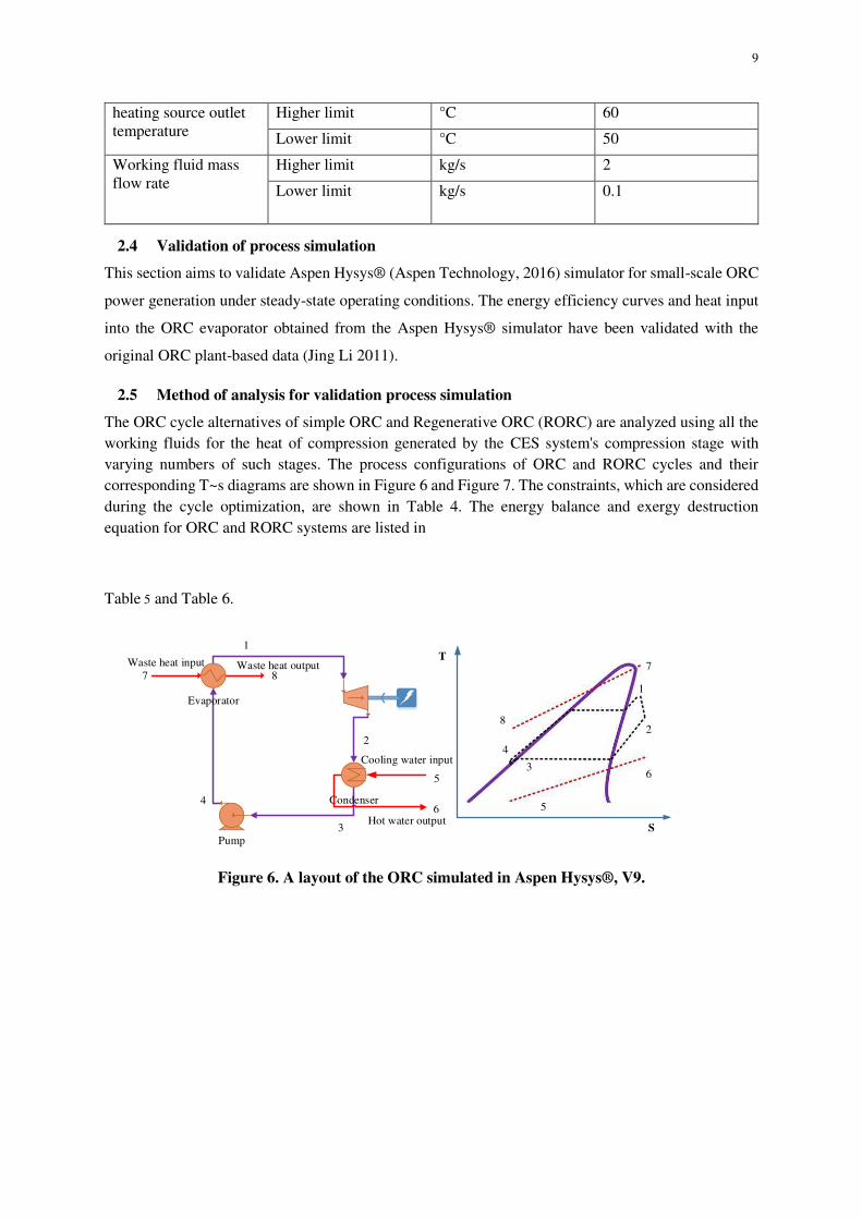
The ORC cycle alternatives of simple ORC and Regenerative ORC (RORC) are analyzed using all the working fluids for the heat of compression generated by the CES system's compression stage with varying numbers of such stages. The process configurations of ORC and RORC cycles and their corresponding T~s diagrams are shown in Figure 6 and Figure 7. The constraints, which are considered

during the cycle optimization, are shown in Table 4. The energy balance and exergy destruction

equation for ORC and RORC systems are listed in

Table 5 and Table 6.

Pump

Condenser

Evaporator

Waste heat input Waste heat output

1

2

3

4

T

S

Cooling water input

Hot water output

5

6

7 8

8

7

6

5

1

2

3

4

Figure 6. A layout of the ORC simulated in Aspen Hysys®, V9.

10

Pump

Condenser

Evaporator

Waste heat input Waste heat output

1

2

3

4

T

S

Cooling water input

Hot water output

5

6

7 8

Recuperator2*

4*

6

5

8

7

1

2

42*

3

4*

Figure 7. A layout of the regenerative cycle simulated in Aspen Hysys®, V9.

Table 4. The parameter used in making the simulation model in Aspen Hysys.

Parameter Value Parameter Value

Hot fluid Flue gas Property package Peng – Robinson Cold fluid Water Pump inlet temperature

(Working fluid) 5°C

The cold source inlet temperature

5°C Pump isentropic efficiency 75%

Cold source outlet temperature

30°C Heat exchanger specification Minimum Approach

Cold source pressure 1500 kPa Expander isentropic efficiency 75% Pinch temperature in the condenser

4ºC Heat exchanger type Shell and Tube

Cold source mass flow rate Dependent Heat exchanger pressure drop 25 kPa The average temperature in Kharagpur (https://en.climate- data.org/location/2825/)

26.7°C Exhaust gas outlet temperature Independent

Economizer effectiveness 0.8 ORC cycles Sub Critical

2.6 Thermodynamic analysis of the ORC and RORC system

Eq. (3) shows the external irreversibilities occurring inside the ORC and RORC system (Roy et al.

2010):

𝐼 = ��𝑇𝑟𝑒𝑓[∑ 𝑠𝑜𝑢𝑡 − ∑ 𝑠𝑖𝑛 + 𝑑𝑠𝑠𝑦𝑠𝑑𝑡 + ∑ 𝑞𝑘𝑇𝑘𝑘 ] (3)

The heat transferred from all heat sources to the working fluid, and Tk refers to the temperature of all

heat sources in Kelvin, m(kg/s) is the total mass flow rate in the cycle, s is entropy state points denoted

as a subscript. Subscripts out and in are the output and input, respectively, of the dedicated stream.

11

Subscript sys represents the ORC and RORC system, and the subscript ref is represented as the reference

temperature. A steady-state of ORC and RORC systems:

𝑑𝑠𝑠𝑦𝑠𝑑𝑡 = 0 (4)

So, Eq. (3) reduces to:

𝐼 = ��𝑇𝑟𝑒𝑓[∑ 𝑠𝑜𝑢𝑡 − ∑ 𝑠𝑖𝑛 + ∑ 𝑞𝑘𝑇𝑘𝑘 ] (5)

For a steady-state, steady flow system, assuming that there are only one inlet and one outlet for each

equipment, Eq. (5) reduces to:

𝐼 = ��𝑇𝑟𝑒𝑓[(𝑠𝑜𝑢𝑡 − 𝑠𝑖𝑛) + 𝑞𝑘𝑇𝑘] (6)

Table 5. Energy balance and exergy destruction equation for ORC system.

Thermodynamic

Process

ORC cycle

component

Energy balance

equations

Equation

Number

Exergy destruction

equations

Equation

Number

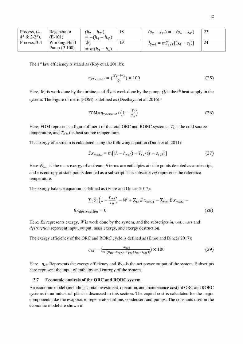
Process, 4-1 Shell and tube heat exchanger (E-100)

��𝑖 = ��(ℎ1 − ℎ4) 7 𝐼4−1 = ��𝑇𝑟𝑒𝑓[(𝑠1 − 𝑠4)+ ℎ4 − ℎ1𝑇𝐻 ] 11

Process, 1-2 Turbo expander (K-100)

��𝑇= ��(ℎ1 − ℎ2) 8 𝐼1−2 = ��𝑇𝑟𝑒𝑓[(𝑠2 − 𝑠1)] 12

Process, 2-3 Condenser(E-101)

��𝑐= ��(ℎ2 − ℎ3) 9 𝐼2−3 = ��𝑇𝑟𝑒𝑓[(𝑠3 − 𝑠2)+ ℎ2 − ℎ3𝑇𝐿 ] 13

Process, 3-4 Working Fluid Pump (P-100)

��𝑝= ��(ℎ3 − ℎ4)

10 𝐼3−4 = ��𝑇𝑟𝑒𝑓[(𝑠4 − 𝑠3)] 14

Table 6. Energy balance and exergy destruction equation for RORC system.

Thermodyn

amic Process

RORC cycle

component

Energy balance

equations

Equation

Number

Exergy destruction rates Equation

Number

Process, 4-1 Shell and tube heat exchanger (E-100)

��𝑖 = ��(ℎ1 − ℎ4) 15 𝐼4∗−1 = ��𝑇𝑟𝑒𝑓[(𝑠1 − 𝑠4∗)+ ℎ4∗ − ℎ1𝑇𝐻 ] 20

Process, 1-2 Turbo expander (K-100).

��𝑇= ��(ℎ1 − ℎ2) 16 𝐼1−2 = ��𝑇𝑟𝑒𝑓[(𝑠2 − 𝑠1)] 21

Process, 2-3 Condenser (E-102)

��𝑐= ��(ℎ4 − ℎ3) 17 𝐼2∗−3 = ��𝑇𝑟𝑒𝑓[(𝑠3 − 𝑠2∗)+ ℎ2∗ − ℎ3𝑇𝐿 ] 22

12

Process, (4-4* & 2-2*),

Regenerator (E-101)

(ℎ2 − ℎ2∗)= −(ℎ4 − ℎ4∗) 18 (𝑠2 − 𝑠2∗) = −(𝑠4 − 𝑠4∗) 23

Process, 3-4 Working Fluid Pump (P-100)

��𝑝= 𝑚(ℎ3 − ℎ4)

19 𝐼3−4 = ��𝑇𝑟𝑒𝑓[(𝑠4 − 𝑠3)] 24

The 1st law efficiency is stated as (Roy et al. 2011b):

𝜂𝑇ℎ𝑒𝑟𝑚𝑎𝑙 = (��𝑇−��𝑃��𝑖 ) × 100 (25)

Here, WT is work done by the turbine, and WP is work done by the pump. Qi is the ith heat supply in the

system. The Figure of merit (FOM) is defined as (Deethayat et al. 2016):

FOM=𝜂𝑇ℎ𝑒𝑟𝑚𝑎𝑙/ (1 − 𝑇𝐿𝑇𝐻) (26)

Here, FOM represents a figure of merit of the total ORC and RORC systems. TL is the cold source

temperature, and TH is the heat source temperature.

The exergy of a stream is calculated using the following equation (Dutta et al. 2011): ��𝑥𝑚𝑎𝑠𝑠 = ��[(ℎ − ℎ𝑟𝑒𝑓) − 𝑇𝑟𝑒𝑓(𝑠 − 𝑠𝑟𝑒𝑓)] (27)

Here massEx& is the mass exergy of a stream, h terms are enthalpies at state points denoted as a subscript,

and s is entropy at state points denoted as a subscript. The subscript ref represents the reference

temperature.

The exergy balance equation is defined as (Emre and Dincer 2017): ∑ ��𝑖𝑖 (1 − 𝑇𝑟𝑒𝑓𝑇𝐻 ) − �� + ∑ ��𝑖𝑛 𝑥𝑚𝑎𝑠𝑠 − ∑ ��𝑜𝑢𝑡 𝑥𝑚𝑎𝑠𝑠 −��𝑥𝑑𝑒𝑠𝑡𝑟𝑢𝑐𝑡𝑖𝑜𝑛 = 0 (28)

Here, Ex represents exergy, W is work done by the system, and the subscripts in, out, mass and

destruction represent input, output, mass exergy, and exergy destruction.

The exergy efficiency of the ORC and RORC cycle is defined as (Emre and Dincer 2017): 𝜂𝑒𝑥 = ( 𝑊𝑛𝑒𝑡��[(ℎ𝑖𝑛−ℎ𝑟𝑒𝑓)−𝑇𝑟𝑒𝑓(𝑠𝑖𝑛−𝑠𝑟𝑒𝑓)]) × 100 (29)

Here, 𝜂𝑒𝑥 Represents the exergy efficiency and Wnet is the net power output of the system. Subscripts here represent the input of enthalpy and entropy of the system.

2.7 Economic analysis of the ORC and RORC system

An economic model (including capital investment, operation, and maintenance cost) of ORC and RORC systems in an industrial plant is discussed in this section. The capital cost is calculated for the major

components like the evaporator, regenerator turbine, condenser, and pumps. The constants used in the

economic model are shown in

13

Table 7. This equipment module costing technique is adapted from (Preißinger et al., 2016), (Özahi et

al., 2018), (Dai et al., 2013). The bare module cost of the equipment is given as follows: 𝐶𝑏𝑚,𝑋 = 𝐶𝑝𝑐,𝑋. 𝐹𝑏,𝑋 (30)

Where 𝐹𝑏,𝑋is the Bare Module Cost factor and is listed in

Table 8. Cpc, X denotes the Purchase Equipment Cost and is expressed as follows: log10𝐶𝑃𝐶,𝑋 = 𝐾1,𝑋 + 𝐾2,𝑋log10𝑌 + 𝐾3,𝑋(log10𝑌)2 (31)

X= Type of equipment, Y= Heat transfer area of the evaporator, condenser and regenerator, and pump

and turbine power capacity. In

Table 8, the equipment cost coefficients 1,XK 2,XK and 3,XK are given (R. Turton, R.C. Bailie 2013).

The total capital cost is as follows: 𝐶total = ∑ 𝐶𝑏𝑚,𝑋 (32)

The Chemical Engineering Plant Cost Index (ICEPC) accounts for issues caused by inflation (Mignard

2014). The ICEPC values obtained from equipment manufacturers for the years 2001 and 2017 are 397

and 632.5 (Saha et al. 2020). The final capital cost of all the equipment is obtained as:

𝐶total,2017 = 𝐶𝑡𝑜𝑡𝑎𝑙.𝐼𝐶𝐸𝑃𝐶,2017𝐼𝐶𝐸𝑃𝐶,2001 (33)

The Capital Recovery Factor (CRF) is obtained as follows:

CRF = 𝑖(1+𝑖)𝑛(1+𝑖)𝑛−1 (34)

where i = interest rate, n = Lifetime of the entire ORC, and RORC system.

The Levelised Energy Cost (LEC) is expressed as follows:

LEC = 𝐶𝑅𝐹.𝐶𝑡𝑜𝑡𝑎𝑙,2017+𝐶𝑜𝑚𝑁.𝑊𝑛𝑒𝑡 (35)

where 𝐶𝑜𝑚 = The operation and maintenance cost, N = Total plant operation hour in one year

14

The Static investment payback period (SIPP) is defined as follows:

SIPP = 𝐶𝑡𝑜𝑡𝑎𝑙,2017+𝐶𝑜𝑚𝐷ℎ𝑟 (36)

where 𝐷ℎ𝑟 = the income per hour by recovering the waste heat for power generation and is stated as

follows: 𝐷ℎ𝑟 = 𝜂𝑃𝑜𝑤𝑒𝑟 . 𝑚ℎ𝑠(ℎℎ𝑖 − ℎℎ𝑜). 𝑃𝑒𝑙𝑒𝑐𝑡𝑟𝑖𝑐𝑖𝑡𝑦 (37) 𝜂𝑃𝑜𝑤𝑒𝑟 = System efficiency, 𝑃𝑒𝑙𝑒𝑐𝑡𝑟𝑖𝑐𝑖𝑡𝑦= Cost of electricity

Table 7. Value of constants used in the economic model

Economic parameter Value N 8000h N 25 years I 5 % 𝐶𝑜𝑚 1.5 𝑃𝑒𝑙𝑒𝑐𝑡𝑟𝑖𝑐𝑖𝑡𝑦 0.342 USD/kWh in San Francisco, CA, USA ORC

(Zhang et al. 2018)

Table 8. The capital cost estimation model with the coefficient (R. Turton, R.C. Bailie 2013).

X Y 𝐾1.𝑋 𝐾2.𝑋 𝐾3.𝑋 𝐹𝑖𝑚.𝑋 Evaporator 𝐴𝑒𝑣𝑎(𝑚)2 4.3247 -0.3030 0.1634 2.9 Condenser 𝐴𝑐𝑜𝑛(𝑚)2 4.3247 -0.3030 0.1634 2.9 Turbine 𝑊𝑇𝑢𝑟𝑏𝑖𝑛𝑒(𝑘𝑊) 2.7051 1.4398 -0.1776 3.5 Pump 𝑊𝑝𝑢𝑚𝑝(𝑘𝑊) 3.3892 0.0536 0.1538 2.8

Regenerator 𝐴𝑟𝑒𝑔(𝑚)2 4.3247 -0.3030 0.1634 2.9

2.8 Heat Exchanger model in Aspen Hysys

Aspen Hysys®, V9 has been used as a script manager for the thermal properties of heat exchangers for

steady-state simulation (Liu and Karimi 2018). The following general relations in Eq. (38) shows,

Balance Error = [��𝑪𝒐𝒍𝒅(𝒉𝒐𝒖𝒕 − 𝒉𝒊𝒏)𝑪𝒐𝒍𝒅 − ��𝒍𝒆𝒂𝒌] − [��𝒉𝒐𝒕(𝒉𝒊𝒏 − 𝒉𝒐𝒖𝒕)𝒉𝒐𝒕 − ��𝒍𝒐𝒔𝒔] (38)

Heat leak, heat loss, Balance Error = a Heat Exchanger Specification that equals zero for most

applications, hot and cold are the hot and cold fluids, in and out is the inlet and outlet stream.

The total heat transferred between the tube and shell sides (Heat Exchanger duty) can be defined in

terms of the overall heat transfer coefficient, the area available for heat exchange and the log mean

temperature difference shown in Eq. (39)

15 𝐐 = 𝐅𝐭 × 𝐔 × 𝐀 × 𝚫𝐓𝐋𝐌𝐓𝐃 (39)

where U is the overall heat transfer coefficient, A is the surface area available for heat transfer, ∆TLM is

the natural log of the mean temperature difference (LMTD), and Ft is the LMTD correction factor

The heat transfer coefficient and the surface area are often combined for convenience into a single

variable referred to as UA. The LMTD and its correction factor are defined in the Performance section.

2.9 Expander model in Aspen Hysys

The expander operation decreases the pressure of a high-pressure inlet gas stream to produce an outlet

stream with low pressure and high velocity. An expansion process involves converting the internal

energy of the gas to kinetic energy and finally to shaft work. For an expander, the efficiency is given as

the ratio of the actual power produced in the expansion process to the power produced for an isentropic

expansion: The expressions are given in Eq. (40) and (41):

Efficiency(%) = (Fluid Power Produced)𝐚𝐜𝐭𝐮𝐚𝐥(Fluid Power Produced)𝐢𝐬𝐞𝐧𝐭𝐫𝐨𝐩𝐢𝐜 × 𝟏𝟎𝟎% (40)

Adiabatic Efficiency = (Work produce𝐝)𝐚𝐜𝐭𝐮𝐚𝐥(Work produce𝐝)𝐢𝐝𝐞𝐚𝐥 = (𝐡𝐨𝐮𝐭−𝐡𝐢𝐧)𝐚𝐜𝐭𝐮𝐚𝐥(𝐡𝐨𝐮𝐭−𝐡𝐢𝐧)𝐢𝐝𝐞𝐚𝐥 (41)

Where h is mass enthalpy, out is product discharge, in is feed stream, P is pressure, in and out is the

inlet and outlet stream.

2.10 Pump model in Aspen Hysys

Calculating the ideal power of the pump required to raise the pressure of the liquid: The calculations

are based on the standard pump equation for power, which uses the pressure rise, the liquid flow rate,

and density:

Powerideal = (𝑃𝑜𝑢𝑡−𝑃𝑖𝑛) × 𝐹𝑙𝑜𝑤𝑟𝑎𝑡𝑒𝐿𝑖𝑞𝑢𝑖𝑑 𝐷𝑒𝑛𝑠𝑖𝑡𝑦 (42)

Where P is pressure and in and out is the inlet and outlet stream.

2.11 Plant configuration and process conditions

The coke oven plant, an ISO 9001-2008 certified company, was founded in 2007 in Kharagpur, West

Bengal, India. BEL has a maximum installed capacity of producing 1.2 million tonnes of coke per

annum through its coke oven and a power generation plant, with a maximum capacity of 80 MW. The

working power production capacity of the combined heat and power (CHP) system in BEL is 40 MW,

with a coke production capacity of 0.6 million tonnes per annum (MTPA). The details related to the

CHP plant are provided in Table 9. The schematic diagram of the actual plant is shown in Figure 8.

16

Sludge transfer pump

Water reservoirClariflocculator

Water Source River

Bore WellPump house

Clarifier water reservoir

CW PUMP Filter Feed pumpWTP

DM tank DM tankBoiler fill pump

CBBT 630CBBT 631

CBBT 632CBBT633

Turbine

Condenser

CEPBFP

FST

P-2

P-3

P-4 P-5

P-6P-7

P-10 P-11

P-13

P-14

P-15

P-17

P-18

P-19

P-20

Cooling tower

P-22

CW PUMPP-23

P-24

P-1

P-12

Figure 8. Schematic diagram of the CHP plant in India

Table 9: CHP Plant Details.

System details Flue gas mass flow rate from coke oven

95000- 110000 N m3/ h / Battery

Production time 24 hour Power used in auxiliary 7-8 % daily power production Power production generator The gas turbine, 40 MW, 11 kVA Type of condenser Cooling towers, Water-cooled condenser Fuels used Natural gas ID fan capacity ID Fan 125 kW x 4 -24 hour running System cogeneration efficiency 90% Local power grid utility WBSEDCL Waste heat temperature 180 ºC SO2 (mg/Nm3) 5.12 CO (mg/Nm3) 4.22 PM (mg/Nm3) 8.52 NOx (mg/Nm3) 16.63 (NOx values are corrected to 15% Oxygen)

17

2.12 Building electricity and cooling loads

The average energy consumption of a commercial building is 61.63 kWh/day, while the average

electricity demand value is 20.12 kWh/day to provide the cooling load of a commercial building. The

daily energy usage of the commercial building during the year 2017 are shown in Figure 9. Figure 10

shows the average mean daily atmospheric temperature over one year in Kharagpur, West Bengal, India,

in hot and humid regions. Figure 11 indicates the required Average system load profile in West Bengal

(2019), India, over one year (IIT Kanpur).

Figure 9. The time-aligned smart meter readings (kWh) the aggregated hourly energy

consumption (kWh) for the commercial load.

Figure 10. Average mean daily air temperature in hot and humid regions in Kharagpur, West

Bengal, India.

0

50

100

150

200

250

300

1-1-1712:00AM

2-1-1712:00AM

3-1-1712:00AM

4-1-1712:00AM

5-1-1712:00AM

6-1-1712:00AM

7-1-1712:00AM

8-1-1712:00AM

9-1-1712:00AM

10-1-1712:00AM

11-1-1712:00AM

12-1-1712:00AM

1-1-1812:00AM

Ene

rgy

Con

sum

tpio

n (k

Wh)

2831

3740 39

3632 31 30 30 29

27

1316

2024

26 27 26 25 2522

1713

2 35

812

35

40

31 32

18

41

Jan Feb Mar Arp May June July Aug Sep Oct Nov Dec

Mean daily maximum °C Mean daily minimum °C Precipitation (mm)

18

Figure 11. Average system load profile West Bengal (2019), India, over one year.

3. Result and discussion

3.1 Comparison of experimental results with simulation

Steady-state simulation of ORC has been performed for the condensation operations based on existing

plant data; the results were compared to energy efficiency and heat input in the evaporator, as shown in

Figure 12 (a) and (b). It has been observed that all the state points and the liquids produce a close match

with those of the plant data, which also authenticate estimation of unknown parameters. Assuming the

direct cool-down sequence, all the steady-state simulations have been executed. There have been some

deviations from simulation, and their causes are listed below.

(a) (b)

Figure 12. Validation of energy efficiency and heat input of experimental data with the

simulation result.

540056005800600062006400660068007000

00:0

0-01

:00

01:0

0-02

:00

02:0

0-03

:00

03:0

0-04

:00

04:0

0-05

:00

05:0

0-06

:00

06:0

0-07

:00

07:0

0-08

:00

08:0

0-09

:00

09:0

0-10

:00

10:0

0-11

:00

11:0

0-12

:00

12:0

0-13

:00

13:0

0-14

:00

14:0

0-15

:00

15:0

0-16

:00

16:0

0-17

:00

17:0

0-18

:00

18:0

0-19

:00

19:0

0-20

:00

20:0

0-21

:00

21:0

0-22

:00

22:0

0-23

:00

23:0

0-24

:00

Demand_weekends (MW) Demand_weekdays (MW)

19

3.1.1 Causes for deviation results in simulation

The simulation result deviations from actual experimental plant data are a common occurrence and its

minimization is the goal of the plant engineer. The main reasons are listed below:

i. The variation of the equipment's material property with respect to temperature has been

manually added; this may not be the best option.

ii. The preloaded numerical method used in Aspen Hysys may not deliver accurate results.

iii. The proper order of cool-down operation of the real plant is unknown.

iv. The expander and pump's isentropic efficiency has changed with the generator rotation speed

variations and input shaft power.

3.1.2 Simulation process: Problems arising in Aspen Hysys®, V9 and solutions

Simulation of an ORC system needs the following features requiring assessment for convergence and

perfection of the simulation result—selecting relevant Equation of State (EOS) to generate fluid

thermodynamic property data.

● Selection of proper transport properties of the working fluids for generating property data.

● Consideration of thermo-physical properties for the insulation and materials.

● Specifications of all the equipment and their performance characteristics.

● Solve the mathematical models of all equipment required in the numerical methods.

● Simple Process flow diagram for reducing the computation time.

3.2 Process modeling and simulation for the CES system

Simulation cases for the selected thermodynamic cycles were developed using a commercial process

simulator, Aspen Hysys®, at steady-state conditions (Dutta et al. 2017a). The Peng-Robinson equation

of state was used for the generation of thermodynamic property data in the simulator. The in-built

models based on energy balance equations for the equipment in the cycle were used. A detailed

discussion of each equipment model for energy and exergy analyses is presented (Dutta et al., 2017a).

The evaporator-superheater in the cycle was modeled using the heater model that supplied heat at a

constant temperature, simplifying the exergy destruction calculations. Parametric studies were

performed using the case study option along with the spreadsheet operation. Exergy destructions in the

cycle and individual equipment were calculated based on the simulation results using Microsoft Excel®.

REFPROP® was used to obtain the enthalpy and entropy data for all the fluids. To keep the references

similar for thermodynamic properties such as enthalpy, entropy, etc., in the calculations, those property

data were estimated using either the simulator or REFPROP®. The flowsheet was built based on the

following assumptions:

1. No pressure drops across the heat exchangers, heater and coolers.

2. Adiabatic efficiencies of compressors, pumps, and turbines are 75%.

3. No heat in-leak in any equipment.

20

4. 100% generator efficiencies.

5. Charging and discharging times are the same.

6. Storage of refrigerants was not considered.

7. No piping and valves were considered in the flowsheet.

8. 50C temperature approach was considered in the thermal energy storage system with 80%

storage efficiency.

3.3 The heat of compression generated during the compression of air in the CES system

The compression stage generally consists of compressors and inter/after coolers. During system

charging, the power is input only to increase the atmosphere's air pressure after filtration. During

compression of air, heat is generated due to the isentropic operation of the compressor. This heat is

dissipated in the atmosphere via cooling using water or air. This, therefore, leads to high exergy

destruction in the liquefier (Thomas 2012). The attempt was made to determine the heat of compression

and the temperature at the compressor's outlet for using this heat to produce power using the

ORC/RORC cycle.

It is known that with an increasing number of stages of compression, the specific power required in the

compressor reduces, as may be seen in Figure 13 (a) and Figure 13 (b) (Thomas 2012). This eventually

reduces the outlet temperature of the compressor and the heat of compression in the process. The

parametric study was performed to determine the heat of compression for multi-stage compression. The

results are shown in Figure 14.

(a) (b)

Figure 13. Variation of specific work required, (b) variation of compressor outlet temperature

with a number of compressor stage with outlet pressure of 150 bar

It is evident from Figure 14 that the temperature at the outlet of the compressors in four stages of

compression is below the typical operating high temperature of an ORC/RORC system. As this system

works for low-grade waste-heat, which is waste-heat at a temperature below 2000C, four-stage of

compression is the choice of a number of compression stages though it may be observed that the specific

21

work required and heat are not far lower for a three-stage compression. Therefore, in this paper, the

heat of compression of the four-stage compression stage was used.

Figure 14. The heat of compression with a number of compression stage in the CES system

The heat of compression with four-stage compression was found to be 2 MW at 450 K temperature.

Therefore, the heat duty for the ORC/RORC cycle was considered as 1.6 MW at 450 K. This is due to

fact that the efficiency of heat storage at the thermal energy storage was assumed to be 80%.

3.4 Optimal compromise solution

Eight various working fluids, namely Butane, Heptane, Hexane, IsoPentane, Neopentane, R-134a, R-

245fa and Toluene, were carefully screened for their thermodynamic behavior. A multi-objective

optimization (MOO) was carried out using an elitist non-dominated sorting genetic sorting algorithm

(NSGA-II) for addressing the conflicting behavior of thermodynamic performance (exergy efficiency,

EXE) and economic performance (Levelized energy cost, LEC). The MOO studies are conducted for

every eight working fluids, and Pareto optimal fronts are generated accordingly. An advanced Pareto

ranking method is known as Grey relation analysis (GRA), and entropy information for weighting the

objectives is considered to select one optimal solution from the Pareto optimal front. Along with this,

an explicit economic performance assessment index, namely the Static Investment Payback Period

(SIPP), is considered to decide the most cost-effective working fluid among the considered fluids. Based

on the obtained results, it is confirmed that R245fa is the most cost-effective working fluid with the

shortest SIPP. Finally, the results suggest that GRA with entropy information considered in this study

can be employed for any possible working fluid to recover low-temperature waste heat in the ORC

(Saha et al. 2019) (Saha et al. 2020). The results are shown in Appendix Figure. A. 1.

3.5 The net power output of ORC and RORC

This work's objective has been to analyze parametrically, compare, and optimize the system power

output. This is based on an optimal mass flow rate with respect to waste heat temperature. We observed

22

that the power output depends on the working fluid's critical pressure (Roy et al. 2011a). As shown in

Figure 15, it was observed that the net power output from the working fluids Butane (18.87 kW, 27.04

kW), Heptane (24.24 kW, 34.03 kW), Hexane (23.30kW, 32.55 kW), Isopentane (19.95 kW,28.18 kW),

Neopentane (16.61kW,23.75 kW) and Toluene (27.23kW, 37.69kW) are comparatively higher for both

ORC and the RORC systems; Eqns. (7) and (15) may be referred to in this regard. Further, power output

for ORC and RORC of R134a (7.73kW, 11.51kW, respectively for ORC and RORC) and R245fa

(9.80kW,13.95kW) are comparatively lower for both ORC and the RORC systems. The variation in the

result may be attributed to changes in enthalpies at the turbine inlet and outlet, with the turbine's

isentropic efficiency being maintained at 75%. Nevertheless, the possible reasons behind the reduction

of the cycle efficiency of the ORC system could be the following:

1. Limiting pressure at the turbine outlet restricted any further reduction of the ORC cycles'

temperatures, leading to an increase in the turbine outlet temperature.

Butane (a) Butane (b)

Heptane (a) Heptane (b)

Hexane (a) Hexane (b)

23

iPentane (a) iPentane (b)

Neopentane (a)

Neopentane (a)

R134a (a)

R134a (a)

R245fa (a) R245fa (b)

24

Toluene (a) Toluene (b)

Figure 15. The net power output of the ORC and the regenerative cycle for different working

fluids

3.6 First law efficiency

Extant literature stated that the regenerative cycle efficiency is higher when compared to the ORC cycle

(Karimi and Mansouri 2018). In a regenerative cycle, using a regenerator is useful for increasing the

power output; this result was compared to other studies in the literature (Roy et al. 2010). Figure 16

exhibits the comparative analysis of first law efficiency between ORC and RORC; the result has been

obtained using Eqn. (25). As shown in Figure 16, it was observed that the cycle efficiency for the

working fluids Butane (11.94 %, 21.38%), Heptane (13.67%, 25.21%), Hexane (13.71%, 24.36%),

Isopentane (12.67%, 22.8%), Neopentane (11.32%, 22.03%) and Toluene (16.06%, 25%) are

comparatively higher for both ORC and the RORC systems. Further, the cycle efficiency of ORC and

RORC of the R134a (10.42%, 19.25%) and R245fa (12.06%, 21.03%) are comparatively lower for both

ORC and the RORC systems. As regards to the RORC system, all hydrocarbons performed better than

CFCs as working fluids.

Butane (a) Butane (b)

25

Heptane (a) Heptane (b)

Hexane (a) Hexane (b)

I-pentane (a) I-pentane (b)

Neopentane (a) Neopentane (b)

26

R134a (a) R134a (b)

R245fa (a) R245fa (b)

Toluene (a) Toluene (b)

Figure 16. The First law efficiency of the ORC and the RORC cycle for different working fluids

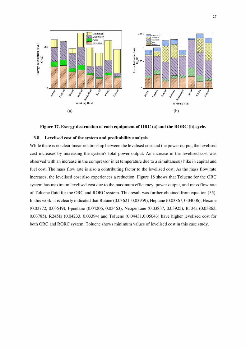
3.7 Exergy destruction analysis

This section covers the assessment of the impact of different operating parameters on the exergy

destruction rate for both the ORC and RORC systems. It is evident from Figure 17 (a) and (b) that the

total exergy destruction is lower in the ORC system in comparison to the RORC system; this result was

derived from the equation for ORC (11-14) and RORC (21-24). It may be noted that the total exergy

loss is proportional to the turbine inlet temperature (TIT) for both the ORC and RORC cycles. The heat

exchanger, gas turbine and condenser are the primary sources for which the exergy destruction increases

with the TIT, mainly due to the heat transfer at higher temperature differences. However, the rise in the

exhaust gas temperature with an increase in TIT acts as a crucial contribution to exergy destruction in

the ORC.

27

(a) (b)

Figure 17. Exergy destruction of each equipment of ORC (a) and the RORC (b) cycle.

3.8 Levelised cost of the system and profitability analysis

While there is no clear linear relationship between the levelised cost and the power output, the levelised

cost increases by increasing the system's total power output. An increase in the levelised cost was

observed with an increase in the compressor inlet temperature due to a simultaneous hike in capital and

fuel cost. The mass flow rate is also a contributing factor to the levelised cost. As the mass flow rate

increases, the levelised cost also experiences a reduction. Figure 18 shows that Toluene for the ORC

system has maximum levelised cost due to the maximum efficiency, power output, and mass flow rate

of Toluene fluid for the ORC and RORC system. This result was further obtained from equation (35).

In this work, it is clearly indicated that Butane (0.03621, 0.03959), Heptane (0.03867, 0.04006), Hexane

(0.03772, 0.03549), I-pentane (0.04206, 0.03463), Neopentane (0.03837, 0.03925), R134a (0.03863,

0.03785), R245fa (0.04233, 0.03394) and Toluene (0.04431,0.05043) have higher levelised cost for

both ORC and RORC system. Toluene shows minimum values of levelised cost in this case study.

28

Figure 18. Comparison of the eight optimal working fluids for Levelised cost of the system and

profitability analysis for both ORC and RORC

3.9 Economic investment and payback period analysis

As shown in Figure 19 (a) and (b), the total cost of the eight working fluids has been compared with

their corresponding efficiency for both the ORC and RORC cycles. In the SIPP calculation, Heptane

shows the highest power generation efficiency and a moderate total cost. The corresponding ranking

performance of the SIPP calculation is reported in Error! Reference source not found.. Additionally,

Cyclohexane is projected as the most cost-effective working fluid for the ORC cycle because its SIPP

is the shortest among the 8 candidates, suggesting that it only takes 102617.46 h to cover the capital

cost and operation and maintenance of the ORC in an ideal situation. With the shortest SIPP among the

eight working fluids, Heptane appears the most cost-effective working fluid for the RORC cycle; it only

takes 55581.382 h to cover the capital cost and operation maintenance of the RORC in an ideal situation.

Compared with the RORC cycle, the ORC system consumes a higher duration to cover the primary

invested value. Here, the SIPP acts as a hypothetical index in the performance ranking of the eight

working fluids in an ideal and identical situation with corresponding economic and thermodynamic

models.

29

Figure 19. Total cost and power generation efficiency of eight working fluid for both ORC (a)

and RORC (b)

Apart from the quality of the system efficiency and levelised cost performances, another primary

concern is the economic benefit explicitly characterized by the SIPP considering the whole ORC

system's total cost and profit. It was found to be a suitable measure for evaluating the effectiveness of

an investment. The SIPP considers the data obtained using Eqn. (36) from the system efficiency and

levelised cost. The shortest SIPP indicates the most cost-effective working fluid. To set a reasonable

criterion for selecting the most cost-effective working fluid, the entire ORC system's SIPP study using

the system efficiency and levelised cost of the optimal compromise solutions for the eight candidates

was taken under consideration.

Figure 20. SIPP Ranking for eight working fluid for both ORC and RORC

30

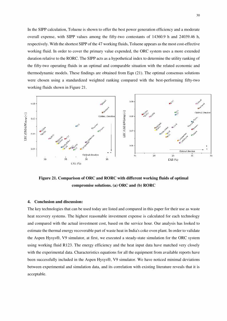
In the SIPP calculation, Toluene is shown to offer the best power generation efficiency and a moderate

overall expense, with SIPP values among the fifty-two contestants of 14360.9 h and 24039.46 h,

respectively. With the shortest SIPP of the 47 working fluids, Toluene appears as the most cost-effective

working fluid. In order to cover the primary value expended, the ORC system uses a more extended

duration relative to the RORC. The SIPP acts as a hypothetical index to determine the utility ranking of

the fifty-two operating fluids in an optimal and comparable situation with the related economic and

thermodynamic models. These findings are obtained from Eqn (21). The optimal consensus solutions

were chosen using a standardized weighted ranking compared with the best-performing fifty-two

working fluids shown in Figure 21.

Figure 21. Comparison of ORC and RORC with different working fluids of optimal

compromise solutions. (a) ORC and (b) RORC

4. Conclusion and discussion:

The key technologies that can be used today are listed and compared in this paper for their use as waste

heat recovery systems. The highest reasonable investment expense is calculated for each technology

and compared with the actual investment cost, based on the service hour. Our analysis has looked to

estimate the thermal energy recoverable part of waste heat in India's coke oven plant. In order to validate

the Aspen Hysys®, V9 simulator, at first, we executed a steady-state simulation for the ORC system

using working fluid R123. The energy efficiency and the heat input data have matched very closely

with the experimental data. Characteristics equations for all the equipment from available reports have

been successfully included in the Aspen Hysys®, V9 simulator. We have noticed minimal deviations

between experimental and simulation data, and its correlation with existing literature reveals that it is

acceptable.

31

Finally, low-grade waste heat recovery technology has a significant potential to be vibrant in the energy

sector; we have looked into the different technical aspects and corresponding challenges. Various

working fluids have also been considered to compare multiple characteristic parameters like first law

efficiency, exergy efficiency, purchase equipment cost, and fixed investment payback period. This

comparative study indicates that the regenerative cycle is the most suitable technique for low grade

waste heat recovery in industrial sectors; additionally, we found that toluene is the most suitable

working fluid based on this particular case study.

This study focused on the power generation potential from low-grade waste heat in an Indian coke oven

plant. No such studies have been found to estimate waste heat potential in energy-intensive industries.

In the future, this method could be employed to assess other energy-intensive sectors, such as iron and

steel, cement, pulp and paper, caustic soda, and glass industries. Nevertheless, we need to mention that

some government reports have covered energy consumption and the process within these energy-

intensive sectors; but there is a severe lack of plant-level information regarding waste heat. For industry

and vehicle motors, variations and intermittency of thermal strength are inherent. Stream management

can ensure safe and near to optimum point operations by bypassing any of the streams in the evaporator.

In order to optimize the quantity of thermal power recovered while reducing energy losses, new

revolutionary technologies can be further developed.

Future research could assess waste heat and its potential conversion to electricity in all pre-discussed

energy-intensive industries. This study for the first time provides a calculation of the thermal energy

potential from the low-temperature waste heat in the coke-oven industry. These types of studies will

assist in achieving the development of sustainable urbanization and a low-carbon footprint. Finally, an

acceptable policy is desired to incorporate waste heat utilization in the world's energy and climate goals.

Declarations

Funding

No funding was received for conducting this study.

Conflict of interest

On behalf of all authors, the corresponding author states that there is no conflict of interest.

Data Availability Statement

Data sharing not applicable to this article as no datasets were generated or analyzed during the current

study.

32

Financial interests

The authors have no relevant financial or non-financial interests to disclose.

References

Acar C, Dincer I (2018) The potential role of hydrogen as a sustainable transportation fuel to combat

global warming. Int J Hydrogen Energy. https://doi.org/10.1016/j.ijhydene.2018.10.149

Agamah SU, Ekonomou L (2017) Energy storage system scheduling for peak demand reduction using

evolutionary combinatorial optimisation. Sustain Energy Technol Assessments 23:73–82.

https://doi.org/10.1016/j.seta.2017.08.003

Bandyopadhyay S, Desai NB (2015) Cost optimal energy sector planning: A Pinch Analysis

approach. J Clean Prod 136:246–253. https://doi.org/10.1016/j.jclepro.2016.03.077

Dai Y, Wang M, Li M, et al (2013) Multi-objective optimization of an organic Rankine cycle (ORC)

for low grade waste heat recovery using evolutionary algorithm. Energy Convers Manag

71:146–158. https://doi.org/10.1016/j.enconman.2013.03.028

Deethayat T, Asanakham A, Kiatsiriroat T (2016) Performance analysis of low temperature organic

Rankine cycle with zeotropic refrigerant by Figure of Merit (FOM). Energy 96:96–102.

https://doi.org/10.1016/j.energy.2015.12.047

Desai NB, Bandyopadhyay S (2015a) Integration of parabolic trough and linear Fresnel collectors for

optimum design of concentrating solar thermal power plant. Clean Technol Environ Policy

17:1945–1961. https://doi.org/10.1007/s10098-015-0918-9

Desai NB, Bandyopadhyay S (2016) Thermo-economic analysis and selection of working fluid for

solar organic Rankine cycle. Appl Therm Eng 95:471–481.

https://doi.org/10.1016/j.applthermaleng.2015.11.018

Desai NB, Bandyopadhyay S (2015b) Optimization of concentrating solar thermal power plant based

on parabolic trough collector. J Clean Prod 89:262–271.

https://doi.org/10.1016/j.jclepro.2014.10.097

Ding Y, Tong L, Zhang P, et al (2016) Chapter 9 - Liquid Air Energy Storage. In: Letcher TM (ed)

Storing Energy. Elsevier, Oxford, pp 167–181

Dutta R, Ghosh P, Chowdhury K (2017a) Process configuration of Liquid-nitrogen Energy Storage

System (LESS) for maximum turnaround efficiency. Cryogenics (Guildf) 88:132–142.

https://doi.org/10.1016/j.cryogenics.2017.10.003

33

Dutta R, Ghosh P, Chowdhury K (2017b) Process configuration of Liquid-nitrogen Energy Storage

System (LESS) for maximum turnaround efficiency. Cryogenics (Guildf) 88:132–142.

https://doi.org/https://doi.org/10.1016/j.cryogenics.2017.10.003

Dutta R, Ghosh P, Chowdhury K (2011) Customization and validation of a commercial process

simulator for dynamic simulation of Helium lique fi er. Energy 36:3204–3214.

https://doi.org/10.1016/j.energy.2011.03.009

Emre M, Dincer I (2017) Development of an integrated hybrid solar thermal power system with

thermoelectric generator for desalination and power production. DES 404:59–71.

https://doi.org/10.1016/j.desal.2016.10.016

European Commission (2018) Paris Agreement

Henriques J, Catarino J (2016) Motivating towards energy efficiency in small and medium

enterprises. J Clean Prod 139:42–50. https://doi.org/10.1016/j.jclepro.2016.08.026

IIT Kanpur KASLPWBEAL EAL (2020). In: Aver. Syst. Load Profile West Bengal, Energy Anal.

Lab, IIT Kanpur, Kanpur. https://eal.iitk.ac.in/download/system_load_profile.php. Accessed 18

Nov 2020

Islam S, Dincer I, Yilbas BS (2018) Development of a novel solar-based integrated system for

desalination with heat recovery. Appl Therm Eng 129:1618–1633.

https://doi.org/10.1016/j.applthermaleng.2017.09.028

Jiménez-Arreola M, Pili R, Dal Magro F, et al (2018) Thermal power fluctuations in waste heat to

power systems: An overview on the challenges and current solutions. Appl Therm Eng 134:576–

584. https://doi.org/10.1016/j.applthermaleng.2018.02.033

Jing Li (2011) Structural Optimization and Experimental Investigation of the Organic Rankine Cycle

for Solar Thermal Power Generation

Kalyanmoy Deb, Amrit Pratap, Sameer Agarwal TM (2002) A Fast and Elitist Multiobjective Genetic

Algorithm: NSGA-II. 182 Ieee Trans Evol Comput 6:182–197.

https://doi.org/10.1109/4235.996017

Karimi S, Mansouri S (2018) A comparative profitability study of geothermal electricity production in

developed and developing countries: Exergoeconomic analysis and optimization of different

ORC configurations. Renew Energy 115:600–619. https://doi.org/10.1016/j.renene.2017.08.098

Krishna B, Basab S (2016) Utilization of low-grade waste heat-to-e.nergy technologies and policy in

Indian industrial sector : a review. Clean Technol Environ Policy.

34

https://doi.org/10.1007/s10098-016-1248-2

Liu Z, Karimi IA (2018) Simulating combined cycle gas turbine power plants in Aspen HYSYS.

Energy Convers Manag 171:1213–1225. https://doi.org/10.1016/j.enconman.2018.06.049

Markides CN (2015) Low-Concentration Solar-Power Systems Based on Organic Rankine Cycles for

Distributed-Scale Applications: Overview and Further Developments. Front Energy Res 3:1–16.

https://doi.org/10.3389/fenrg.2015.00047

Mignard D (2014) Correlating the chemical engineering plant cost index with macro-economic

indicators. Chem Eng Res Des 92:285–294. https://doi.org/10.1016/j.cherd.2013.07.022

Minea V (2014) Power generation with ORC machines using low-grade waste heat or renewable

energy. Appl Therm Eng 69:143–154. https://doi.org/10.1016/j.applthermaleng.2014.04.054

Morgan R, Nelmes S, Gibson E, Brett G (2015) Liquid air energy storage – Analysis and first results

from a pilot scale demonstration plant. Appl Energy 137:845–853.

https://doi.org/10.1016/j.apenergy.2014.0

National Productivity Council I (2017) GHG-Manual-Thermal-Power-Plant.

https://www.npcindia.gov.in/NPC/User/index. Accessed 6 Jul 2020

Özahi E, Tozlu A, Abuşoğlu A (2018) Thermoeconomic multi-objective optimization of an organic

Rankine cycle (ORC) adapted to an existing solid waste power plant. Energy Convers Manag

168:308–319. https://doi.org/10.1016/j.enconman.2018.04.103

Parrondo AJ, Villar A, Jose J (2012) Waste-to-energy technologies in continuous process industries.

29–39. https://doi.org/10.1007/s10098-011-0385-x

Preißinger M, Schatz S, Vogl A, et al (2016) Thermoeconomic analysis of configuration methods for

modular Organic Rankine Cycle units in low-temperature applications. 127:25–34.

https://doi.org/10.1016/j.enconman.2016.08.092

Priya GSK, Bandyopadhyay S (2013) Emission constrained power system planning : a pinch analysis

based study of Indian electricity sector. 771–782. https://doi.org/10.1007/s10098-012-0541-y

R. Turton, R.C. Bailie WBW and JAS (2013) Analysis, synthesis, and design of chemical processes

Rezvani A, Gandomkar M, Izadbakhsh M, Ahmadi A (2015) Environmental / economic scheduling of

a micro-grid with renewable energy resources. J Clean Prod 87:216–226.

https://doi.org/10.1016/j.jclepro.2014.09.088

Roy JP, Mishra MK, Misra A (2011a) Performance analysis of an Organic Rankine Cycle with

35

superheating under different heat source temperature conditions. Appl Energy 88:2995–3004.

https://doi.org/10.1016/j.apenergy.2011.02.042

Roy JP, Mishra MK, Misra A (2010) Parametric optimization and performance analysis of a waste

heat recovery system using Organic Rankine Cycle. Energy 35:5049–5062.

https://doi.org/10.1016/j.energy.2010.08.013

Roy JP, Mishra MK, Misra A (2011b) Performance analysis of an Organic Rankine Cycle with

superheating under different heat source temperature conditions. Appl Energy 88:2995–3004.

https://doi.org/10.1016/j.apenergy.2011.02.042

Sadeghi M, Kalantar M (2015) The analysis of the effects of clean technologies from economic point

of view. J Clean Prod 102:394–407. https://doi.org/10.1016/j.jclepro.2015.04.042

Saha BK, Chakraborty B, Dutta R (2020) Estimation of waste heat and its recovery potential from

energy-intensive industries. Clean Technol Environ Policy 22:1795–1814.

https://doi.org/10.1007/s10098-020-01919-7

Saha BK, Chakraborty B, Pundeer P (2019) Thermodynamic and thermo economic analysis of

organic rankine cycle with multi-objective optimization for working fluid selection with low-

temperature waste sources in the Indian industry. 5th Int Semin ORC Power Syst 5–12

Sarkar J, Bhattacharyya S (2015a) Potential of organic Rankine cycle technology in India: Working

fluid selection and feasibility study. Energy 90:1618–1625.

https://doi.org/10.1016/j.energy.2015.07.001

Sarkar J, Bhattacharyya S (2015b) Potential of organic Rankine cycle technology in India : Working fl

uid selection and feasibility study. Energy 90:1618–1625.

https://doi.org/10.1016/j.energy.2015.07.001

Shin-Ichi Inage (2009) Prospects for Energy Storage in Decarbonised Power Grids WO R K I N G PA

P E R. 92

Sikdar SK, Sengupta D, Mukherjee R (2017) Measuring Progress Towards Sustainability. Springer

International Publishing

Tafone A, Borri E, Comodi G, et al (2017) Preliminary assessment of waste heat recovery solution

(ORC) to enhance the performance of Liquid Air Energy Storage system. In: Energy Procedia.

Elsevier Ltd, pp 3609–3616

The MathWorks Inc 2018 (2018) MATLAB

36

Thomas RJ (2012) Exergy approach in designing large-scale helium liquefiers. Indian Institute of

Technology Kharagpur, India

Xie C, Li Y, Ding Y, Radcliffe J (2019) Evaluating Levelized Cost of Storage (LCOS) Based on Price

Arbitrage Operations: with Liquid Air Energy Storage (LAES) as an Example. Energy Procedia

158:4852–4860. https://doi.org/https://doi.org/10.1016/j.egypro.2019.01.708

Zhang Z, Zhang X, Bai H, et al (2018) Multi-objective optimisation and fast decision-making method

for working fluid selection in organic Rankine cycle with low-temperature waste heat source in

industry. Energy Convers Manag 172:200–211. https://doi.org/10.1016/j.enconman.2018.07.021

Supplementary Files

This is a list of supplementary �les associated with this preprint. Click to download.

GraphicalAbstract.docx

SupplementaryMaterial.docx