Add-on Module STEEL BS - Dlubal · PDF fileAdd-on Module STEEL BS ... BS 5950-1 and BS EN...

Program STEEL BS © 2011 by Ing. Software Dlubal

Add-on Module

STEEL BS Ultimate Limit State and Service-ability Limit State Design acc. to BS 5950-1 and BS EN 1993-1-1

Program Description

Version September 2011

All rights, including those of the translation, are reserved. No portion of this book may be reproduced – mechanically, electronically, or by any other means, including photocopying – without written permission of ING. SOFTWARE DLUBAL. © Ing. Software Dlubal

Am Zellweg 2 D - 93464 Tiefenbach

Tel: +49 (0) 9673 9203-0 Fax: +49 (0) 9673 9203-51 E-mail: [email protected] Web: www.dlubal.com

3

Contents

Contents Page

Contents Page

Program STEEL BS © 2011 by Ing. Software Dlubal

1. Introduction 4 1.1 Additional Module STEEL BS 4 1.2 STEEL BS Team 5 1.3 Using the Manual 5 1.4 Starting STEEL BS 6 2. Input Data 8 2.1 General Data 8 2.1.1 Ultimate Limit State 8 2.1.2 Serviceability Limit State 10 2.1.3 National Annex (NA) 11 2.2 Materials 14 2.3 Cross-Sections 16 2.4 Lateral Intermediate Supports 20 2.5 Effective Lengths - Members 21 2.6 Effective Lengths - Sets of Members 24 2.7 Nodal Supports 25 2.8 Member Releases 27 2.9 Serviceability Data 28 3. Calculation 29 3.1 Details 29 3.2 Start Calculation 31 4. Results 33 4.1 Design by Load Case 33 4.2 Design by Cross-Section 34 4.3 Design by Set of Members 35 4.4 Design by Member 35 4.5 Design by x-Location 36 4.6 Governing Internal Forces by Member 37 4.7 Governing Internal Forces by Set of

Members 38 4.8 Member Slendernesses 38 4.9 Parts List by Member 39 4.10 Parts List by Set of Members 40 5. Evaluation of Results 41 5.1 Results on RSTAB Model 42 5.2 Result Diagrams 46 5.3 Filter Results 47

6. Printout 49 6.1 Printout Report 49 6.2 Print STEEL BS Graphics 49 7. General Functions 51 7.1 STEEL BS Design Cases 51 7.2 Cross-Section Optimization 53 7.3 Import / Export of Materials 55 7.4 Units and Decimal Places 56 7.5 Export Results 56 8. Example 58 A Literature 67 B Index 68

1 Introduction

4 Program STEEL BS © 2011 by Ing. Software Dlubal

1. Introduction

1.1 Additional Module STEEL BS

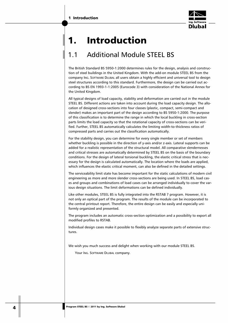
The British Standard BS 5950-1:2000 determines rules for the design, analysis and construc-tion of steel buildings in the United Kingdom. With the add-on module STEEL BS from the company ING. SOFTWARE DLUBAL all users obtain a highly efficient and universal tool to design steel structures according to this standard. Furthermore, the design can be carried out ac-cording to BS EN 1993-1-1:2005 (Eurocode 3) with consideration of the National Annex for the United Kingdom.

All typical designs of load capacity, stability and deformation are carried out in the module STEEL BS. Different actions are taken into account during the load capacity design. The allo-cation of designed cross-sections into four classes (plastic, compact, semi-compact and slender) makes an important part of the design according to BS 5950-1:2000. The purpose of this classification is to determine the range in which the local buckling in cross-section parts limits the load capacity so that the rotational capacity of cross-sections can be veri-fied. Further, STEEL BS automatically calculates the limiting width-to-thickness ratios of compressed parts and carries out the classification automatically.

For the stability design, you can determine for every single member or set of members whether buckling is possible in the direction of y-axis and/or z-axis. Lateral supports can be added for a realistic representation of the structural model. All comparative slendernesses and critical stresses are automatically determined by STEEL BS on the basis of the boundary conditions. For the design of lateral torsional buckling, the elastic critical stress that is nec-essary for the design is calculated automatically. The location where the loads are applied, which influences the elastic critical moment, can also be defined in the detailed settings.

The serviceability limit state has become important for the static calculations of modern civil engineering as more and more slender cross-sections are being used. In STEEL BS, load cas-es and groups and combinations of load cases can be arranged individually to cover the var-ious design situations. The limit deformations can be defined individually.

Like other modules, STEEL BS is fully integrated into the RSTAB 7 program. However, it is not only an optical part of the program. The results of the module can be incorporated to the central printout report. Therefore, the entire design can be easily and especially uni-formly organized and presented.

The program includes an automatic cross-section optimization and a possibility to export all modified profiles to RSTAB.

Individual design cases make it possible to flexibly analyze separate parts of extensive struc-tures.

We wish you much success and delight when working with our module STEEL BS.

Your ING. SOFTWARE DLUBAL company.

1 Introduction


1.2 STEEL BS Team The following people participated in the development of the STEEL BS module:

Program Coordinators Dipl.-Ing. Georg Dlubal Dipl.-Ing. (FH) Younes El Frem

Ing. Ph.D. Peter Chromiak

Programmers Ing. Zdeněk Kosáček Ing. Ph.D. Peter Chromiak Dipl.-Ing. Georg Dlubal Dr.-Ing. Jaroslav Lain Ing. Martin Budáč

Mgr. Petr Oulehle Ing. Roman Svoboda David Schweiner Ing. Zbyněk Zámečník DiS. Jiří Šmerák

Library of Cross-Sections and Materials Ing. Ph.D. Jan Rybín Stanislav Krytinář

Jan Brnušák

Design of Program, Dialog Boxes and Icons Dipl.-Ing. Georg Dlubal MgA. Robert Kolouch

Ing. Jan Miléř

Testing and Technical Support Ing. Ctirad Martinec Ing. Martin Vasek Ing. Ph.D. Peter Chromiak Dipl.-Ing. (FH) René Flori Dipl.-Ing. (FH) Matthias Entenmann Dipl.-Ing. Frank Faulstich

M. Sc. Dipl.-Ing. (FH) Frank Lobisch Dipl.-Ing. (BA) Andreas Niemeier Dipl.-Ing. (FH) Walter Rustler M. Sc. Dipl.-Ing. (FH) Frank Sonntag Dipl.-Ing. (FH) Christian Stautner Dipl.-Ing. (FH) Robert Vogl

Manuals, Documentation and Translations Ing. Ph.D. Peter Chromiak Dipl.-Ing. (FH) Robert Vogl Mgr. Petra Pokorná Ing. Petr Míchal

Ing. Ladislav Kábrt Ing. Dmitry Bystrov Mgr. Michaela Kryšková

1.3 Using the Manual All general topics such as installation, user interface, results evaluation and printout report are described in detail in the manual for the main program RSTAB. Hence, we omit them in this manual and will focus on typical features of the add-on module STEEL BS.

During the description of STEEL BS, we use the sequence and structure of the different in-put and output tables. We feature the described icons (buttons) in square brackets, e.g. [Pick]. The buttons are simultaneously displayed on the left margin. The names of dialog boxes, tables and particular menus are marked in italics in the text so that they can be easily found in the program.

The index at the end of this manual enables you to quickly look up specific terms.

1 Introduction


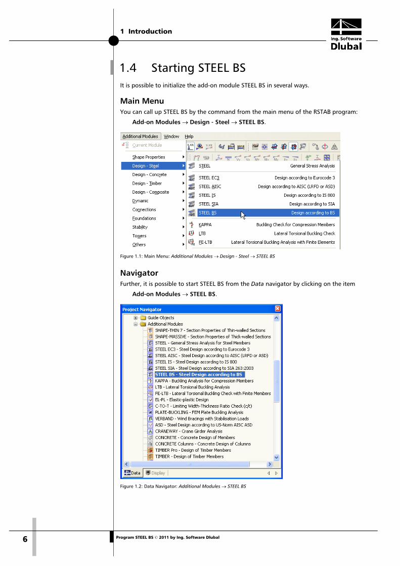
1.4 Starting STEEL BS It is possible to initialize the add-on module STEEL BS in several ways.

Main Menu You can call up STEEL BS by the command from the main menu of the RSTAB program:

Add-on Modules → Design - Steel → STEEL BS.

Figure 1.1: Main Menu: Additional Modules → Design - Steel → STEEL BS

Navigator Further, it is possible to start STEEL BS from the Data navigator by clicking on the item

Add-on Modules → STEEL BS.

Figure 1.2: Data Navigator: Additional Modules → STEEL BS

1 Introduction


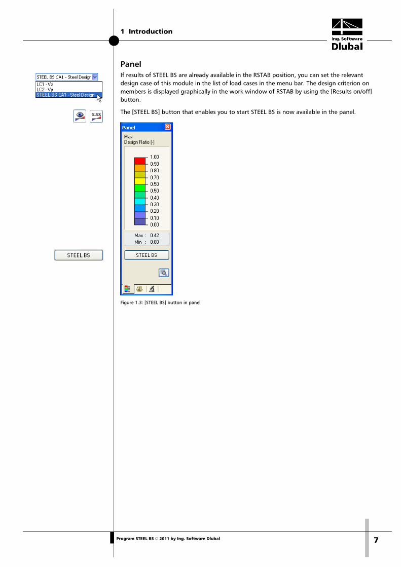
Panel If results of STEEL BS are already available in the RSTAB position, you can set the relevant design case of this module in the list of load cases in the menu bar. The design criterion on members is displayed graphically in the work window of RSTAB by using the [Results on/off] button.

The [STEEL BS] button that enables you to start STEEL BS is now available in the panel.

Figure 1.3: [STEEL BS] button in panel

2 Input Data


2. Input Data The data of the design cases is to be entered in different tables of the module. Furthermore, the graphic input using the function [Pick] is available for members and sets of members.

After the initialization of the STEEL BS module, a new window is displayed. In its left part, a navigator is shown that enables you to access all existing tables. The roll-out list of all pos-sibly entered design cases is located above this navigator (see chapter 7.1, page 51).

If STEEL BS is called up for the first time in a position of RSTAB, the following important da-ta is loaded automatically:

• Members and sets of members • Load cases, load groups and combinations • Materials • Cross-sections • Internal forces (in the background – if calculated)

You can switch among the tables either by clicking on the individual navigator items of STEEL BS or by using the buttons visible on the left. The [F2] and [F3] function keys can also be used to browse the tables in both directions.

Save entered data by the [OK] button and close the module STEEL BS, while by the [Cancel] button you terminate the module without saving data.

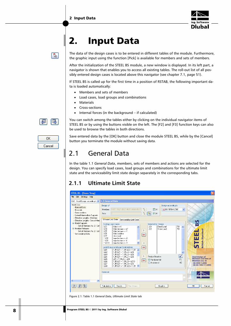
2.1 General Data In the table 1.1 General Data, members, sets of members and actions are selected for the design. You can specify load cases, load groups and combinations for the ultimate limit state and the serviceability limit state design separately in the corresponding tabs.

2.1.1 Ultimate Limit State

Figure 2.1: Table 1.1 General Data, Ultimate Limit State tab

2 Input Data


Design of You can select both Members and Sets of Members for the design. If only specific objects are to be designed, it is necessary to clear the check box All. By doing so, both input boxes become accessible and you can enter the numbers of the relevant members or sets of mem-bers there. With the [Pick] button, you can also select members or sets of members graph-ically in the RSTAB work window. To rewrite the list of default member numbers, select it by double-clicking it, and then enter the relevant numbers.

If no sets of members have been defined in RSTAB yet, they can be created in STEEL BS via the [New Set of Members…] button. The familiar RSTAB dialog box to create a new set of members opens in which you enter the relevant data.

Designing sets of members has the advantage that selected members can be analyzed to determine the total maxima of the design ratios. In this case, the results tables 2.3 Design by Set of Members, 3.2 Governing Internal Forces by Set of Members and 4.2 Parts List by Set of Members are displayed additionally.

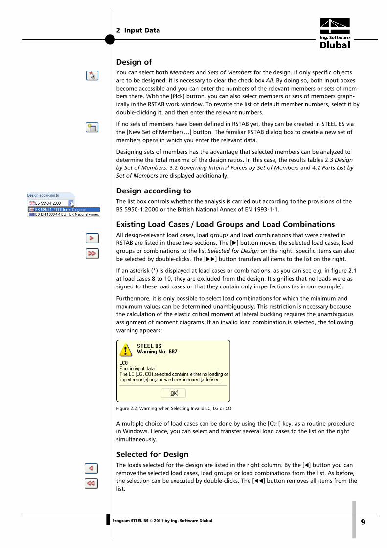
Design according to The list box controls whether the analysis is carried out according to the provisions of the BS 5950-1:2000 or the British National Annex of EN 1993-1-1.

Existing Load Cases / Load Groups and Load Combinations All design-relevant load cases, load groups and load combinations that were created in RSTAB are listed in these two sections. The [] button moves the selected load cases, load groups or combinations to the list Selected for Design on the right. Specific items can also be selected by double-clicks. The [] button transfers all items to the list on the right.

If an asterisk (*) is displayed at load cases or combinations, as you can see e.g. in figure 2.1 at load cases 8 to 10, they are excluded from the design. It signifies that no loads were as-signed to these load cases or that they contain only imperfections (as in our example).

Furthermore, it is only possible to select load combinations for which the minimum and maximum values can be determined unambiguously. This restriction is necessary because the calculation of the elastic critical moment at lateral buckling requires the unambiguous assignment of moment diagrams. If an invalid load combination is selected, the following warning appears:

Figure 2.2: Warning when Selecting Invalid LC, LG or CO

A multiple choice of load cases can be done by using the [Ctrl] key, as a routine procedure in Windows. Hence, you can select and transfer several load cases to the list on the right simultaneously.

Selected for Design The loads selected for the design are listed in the right column. By the [] button you can remove the selected load cases, load groups or load combinations from the list. As before, the selection can be executed by double-clicks. The [] button removes all items from the list.

2 Input Data


Generally, the calculation of an enveloping Or load combination is faster than the analysis of all contained load cases or groups. On the other hand, you must keep in mind the above-mentioned restriction: to determine the maximum or minimum values unambiguously, the Or load combination must only contain load cases, groups or combinations which enter the combination with the criterion Constant. Moreover, the design of an enveloping load com-bination makes it a bit difficult to retrace the influence of the contained actions.

2.1.2 Serviceability Limit State

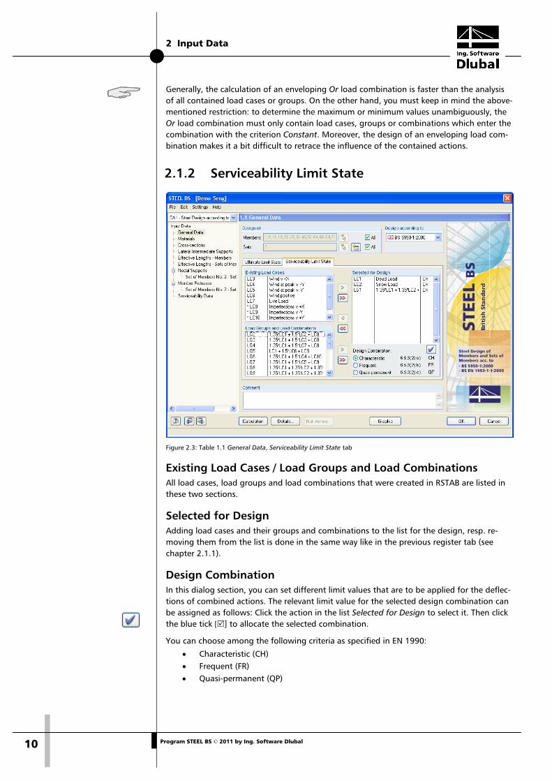
Figure 2.3: Table 1.1 General Data, Serviceability Limit State tab

Existing Load Cases / Load Groups and Load Combinations All load cases, load groups and load combinations that were created in RSTAB are listed in these two sections.

Selected for Design Adding load cases and their groups and combinations to the list for the design, resp. re-moving them from the list is done in the same way like in the previous register tab (see chapter 2.1.1).

Design Combination In this dialog section, you can set different limit values that are to be applied for the deflec-tions of combined actions. The relevant limit value for the selected design combination can be assigned as follows: Click the action in the list Selected for Design to select it. Then click the blue tick [] to allocate the selected combination.

You can choose among the following criteria as specified in EN 1990:

• Characteristic (CH) • Frequent (FR) • Quasi-permanent (QP)

2 Input Data


The limit values are settled by the standard. They can be modified in the dialog box that controls the details (see figure 3.1, page 29) resp. the parameters of the National Annex (see figure 2.4, page 11).

Comment You can enter some additional notes here to describe the current design case.

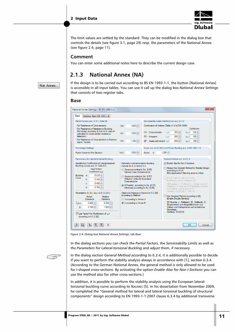
2.1.3 National Annex (NA) If the design is to be carried out according to BS EN 1993-1-1, the button [National Annex] is accessible in all input tables. You can use it call up the dialog box National Annex Settings that consists of two register tabs.

Base

Figure 2.4: Dialog box National Annex Settings, tab Base

In the dialog sections you can check the Partial Factors, the Serviceability Limits as well as the Parameters for Lateral-torsional Buckling and adjust them, if necessary.

In the dialog section General Method according to 6.3.4, it is additionally possible to decide if you want to perform the stability analysis always in accordance with [1], section 6.3.4. (According to the German National Annex, the general method is only allowed to be used for I-shaped cross-sections. By activating the option Enable Also for Non I-Sections you can use the method also for other cross-sections.)

In addition, it is possible to perform the stability analysis using the European lateral-torsional buckling curve according to NAUMES [5]. In his dissertation from November 2009, he completed the “General method for lateral and lateral torsional buckling of structural components” design according to EN 1993-1-1:2007 clause 6.3.4 by additional transverse

2 Input Data


bending and torsion. This method is available in STEEL BS in order to design unsymmetrical cross-sections as well as tapered members and sets of members with biaxial bending.

According to section 6.3.4 (4), the reduction factor χop is to be calculated

a) as minimum value of the values for buckling according to 6.3.1 or χLT for lateral-torsional buckling according to 6.3.2 by means of the slenderness degree χop , or

b) as a value that is interpolated between χ and χLT (see also equation (6.66) of EN 1993-1-1).

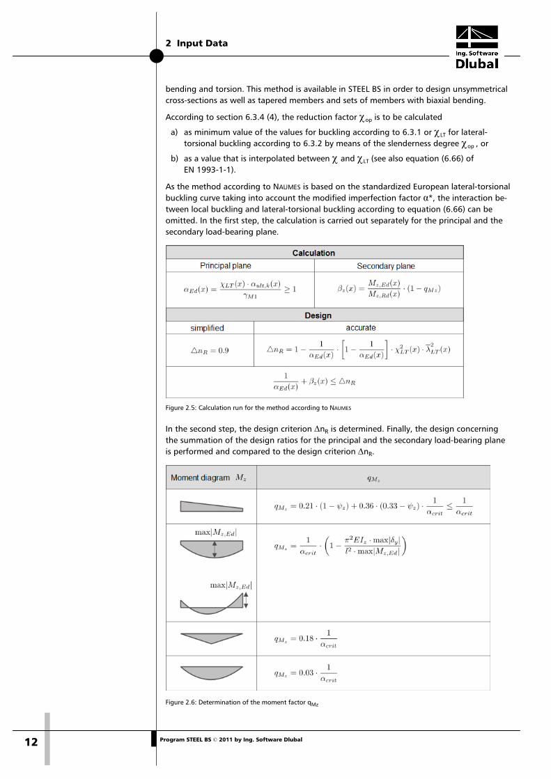
As the method according to NAUMES is based on the standardized European lateral-torsional buckling curve taking into account the modified imperfection factor α*, the interaction be-tween local buckling and lateral-torsional buckling according to equation (6.66) can be omitted. In the first step, the calculation is carried out separately for the principal and the secondary load-bearing plane.

Figure 2.5: Calculation run for the method according to NAUMES

In the second step, the design criterion ∆nR is determined. Finally, the design concerning the summation of the design ratios for the principal and the secondary load-bearing plane is performed and compared to the design criterion ∆nR.

Figure 2.6: Determination of the moment factor qMz

2 Input Data


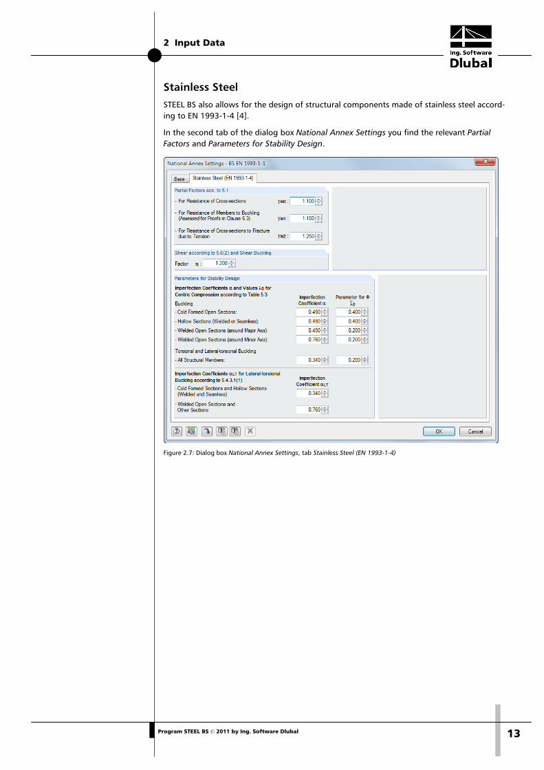
Stainless Steel STEEL BS also allows for the design of structural components made of stainless steel accord-ing to EN 1993-1-4 [4].

In the second tab of the dialog box National Annex Settings you find the relevant Partial Factors and Parameters for Stability Design.

Figure 2.7: Dialog box National Annex Settings, tab Stainless Steel (EN 1993-1-4)

2 Input Data


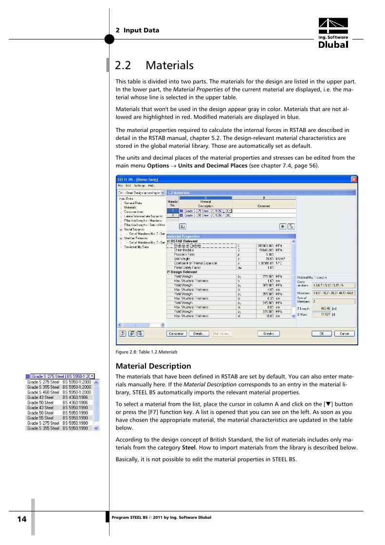
2.2 Materials This table is divided into two parts. The materials for the design are listed in the upper part. In the lower part, the Material Properties of the current material are displayed, i.e. the ma-terial whose line is selected in the upper table.

Materials that won't be used in the design appear gray in color. Materials that are not al-lowed are highlighted in red. Modified materials are displayed in blue.

The material properties required to calculate the internal forces in RSTAB are described in detail in the RSTAB manual, chapter 5.2. The design-relevant material characteristics are stored in the global material library. Those are automatically set as default.

The units and decimal places of the material properties and stresses can be edited from the main menu Options → Units and Decimal Places (see chapter 7.4, page 56).

Figure 2.8: Table 1.2 Materials

Material Description The materials that have been defined in RSTAB are set by default. You can also enter mate-rials manually here. If the Material Description corresponds to an entry in the material li-brary, STEEL BS automatically imports the relevant material properties.

To select a material from the list, place the cursor in column A and click on the [] button or press the [F7] function key. A list is opened that you can see on the left. As soon as you have chosen the appropriate material, the material characteristics are updated in the table below.

According to the design concept of British Standard, the list of materials includes only ma-terials from the category Steel. How to import materials from the library is described below.

Basically, it is not possible to edit the material properties in STEEL BS.

2 Input Data


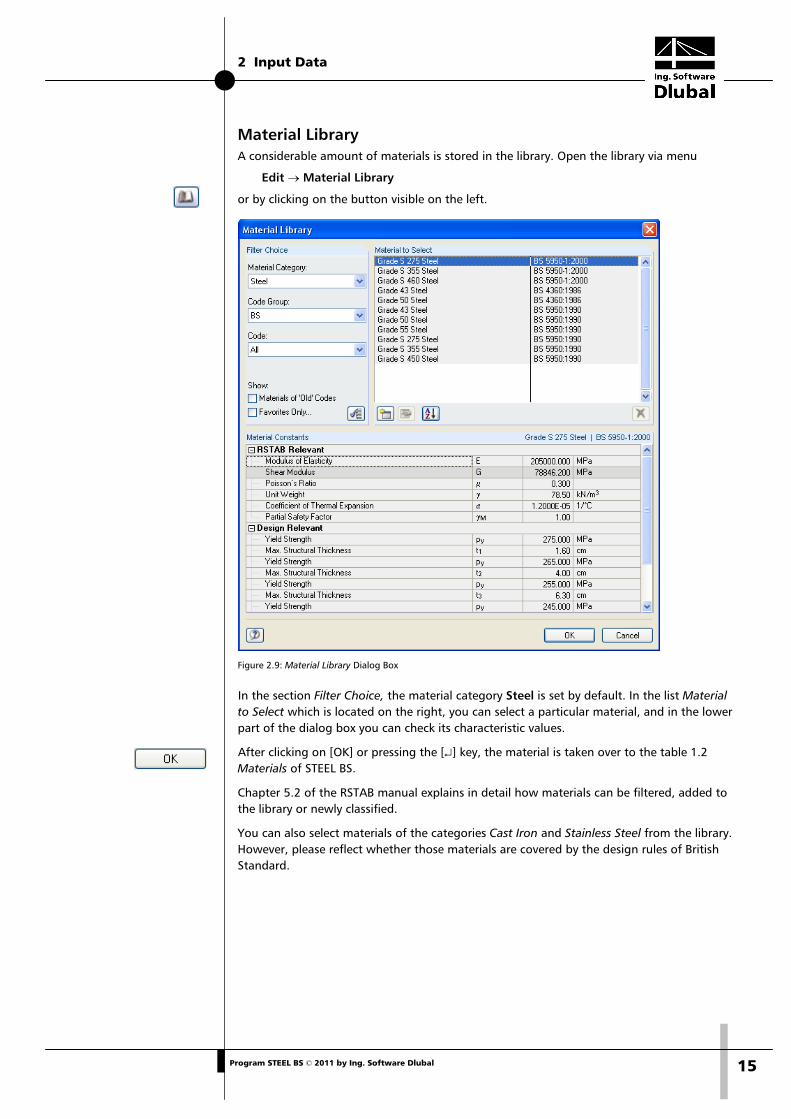
Material Library A considerable amount of materials is stored in the library. Open the library via menu

Edit → Material Library

or by clicking on the button visible on the left.

Figure 2.9: Material Library Dialog Box

In the section Filter Choice, the material category Steel is set by default. In the list Material to Select which is located on the right, you can select a particular material, and in the lower part of the dialog box you can check its characteristic values.

After clicking on [OK] or pressing the [↵] key, the material is taken over to the table 1.2 Materials of STEEL BS.

Chapter 5.2 of the RSTAB manual explains in detail how materials can be filtered, added to the library or newly classified.

You can also select materials of the categories Cast Iron and Stainless Steel from the library. However, please reflect whether those materials are covered by the design rules of British Standard.

2 Input Data


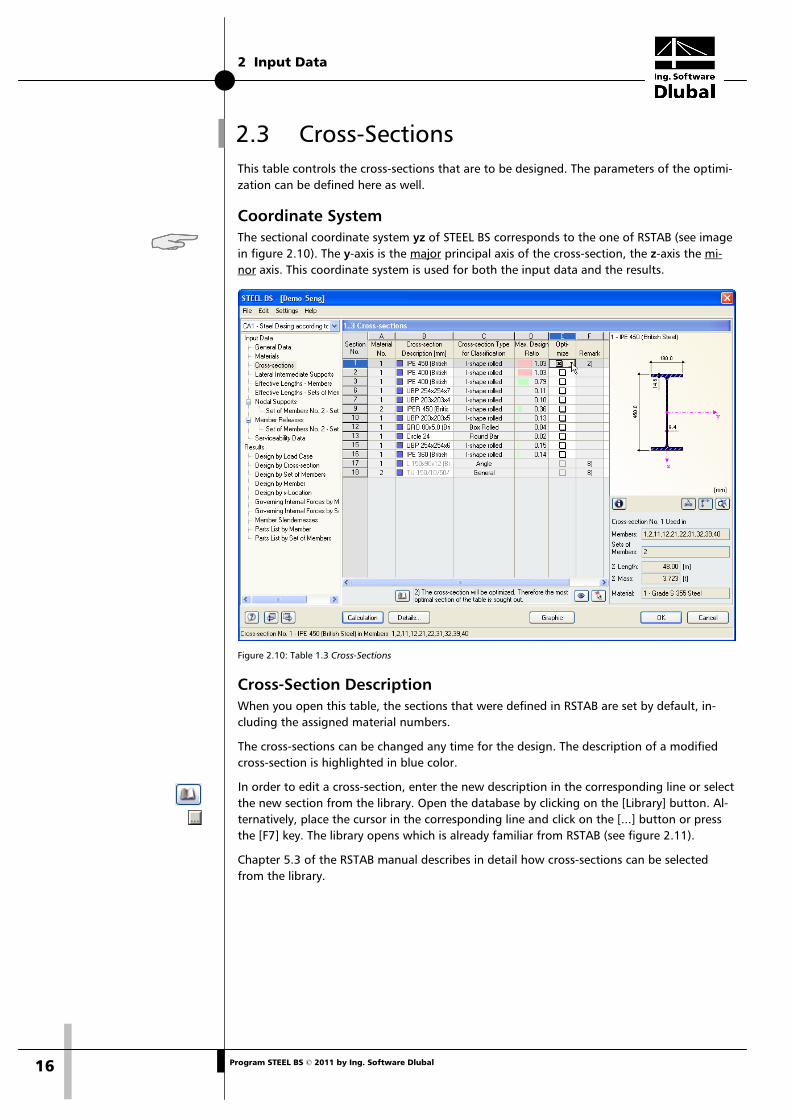
2.3 Cross-Sections This table controls the cross-sections that are to be designed. The parameters of the optimi-zation can be defined here as well.

Coordinate System The sectional coordinate system yz of STEEL BS corresponds to the one of RSTAB (see image in figure 2.10). The y-axis is the major principal axis of the cross-section, the z-axis the mi-nor axis. This coordinate system is used for both the input data and the results.

Figure 2.10: Table 1.3 Cross-Sections

Cross-Section Description When you open this table, the sections that were defined in RSTAB are set by default, in-cluding the assigned material numbers.

The cross-sections can be changed any time for the design. The description of a modified cross-section is highlighted in blue color.

In order to edit a cross-section, enter the new description in the corresponding line or select the new section from the library. Open the database by clicking on the [Library] button. Al-ternatively, place the cursor in the corresponding line and click on the [...] button or press the [F7] key. The library opens which is already familiar from RSTAB (see figure 2.11).

Chapter 5.3 of the RSTAB manual describes in detail how cross-sections can be selected from the library.

2 Input Data


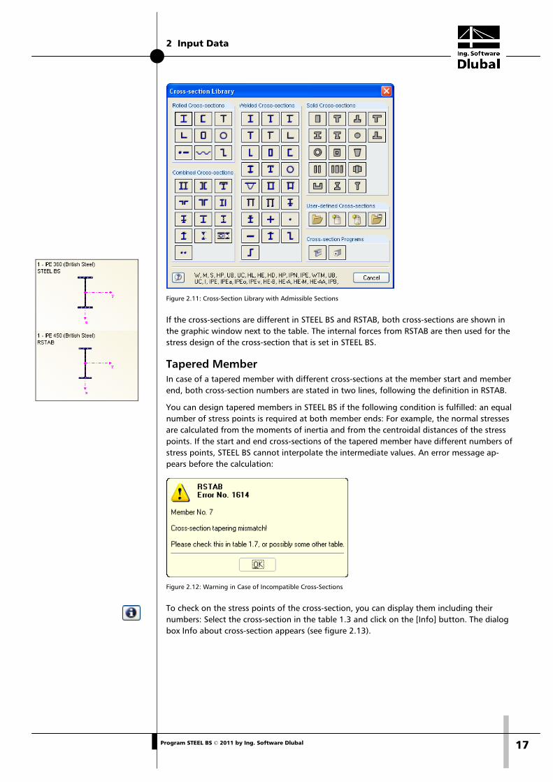
Figure 2.11: Cross-Section Library with Admissible Sections

If the cross-sections are different in STEEL BS and RSTAB, both cross-sections are shown in the graphic window next to the table. The internal forces from RSTAB are then used for the stress design of the cross-section that is set in STEEL BS.

Tapered Member In case of a tapered member with different cross-sections at the member start and member end, both cross-section numbers are stated in two lines, following the definition in RSTAB.

You can design tapered members in STEEL BS if the following condition is fulfilled: an equal number of stress points is required at both member ends: For example, the normal stresses are calculated from the moments of inertia and from the centroidal distances of the stress points. If the start and end cross-sections of the tapered member have different numbers of stress points, STEEL BS cannot interpolate the intermediate values. An error message ap-pears before the calculation:

Figure 2.12: Warning in Case of Incompatible Cross-Sections

To check on the stress points of the cross-section, you can display them including their numbers: Select the cross-section in the table 1.3 and click on the [Info] button. The dialog box Info about cross-section appears (see figure 2.13).

2 Input Data


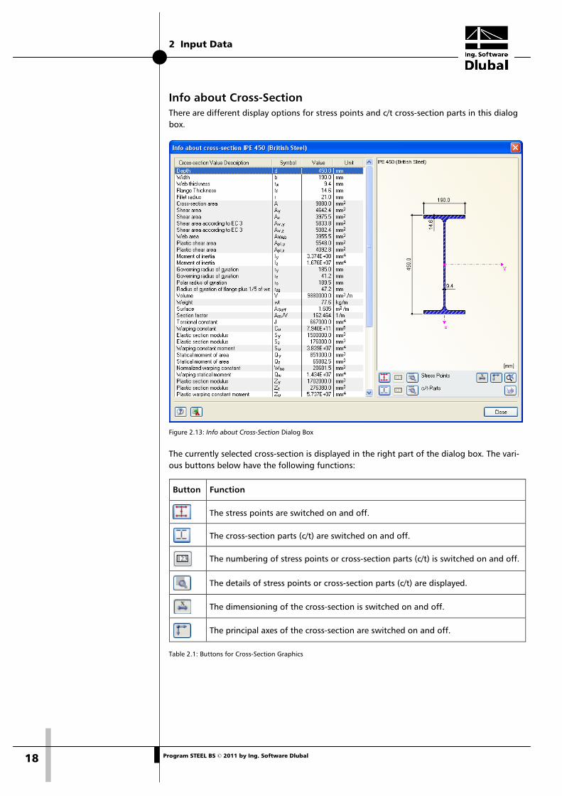
Info about Cross-Section There are different display options for stress points and c/t cross-section parts in this dialog box.

Figure 2.13: Info about Cross-Section Dialog Box

The currently selected cross-section is displayed in the right part of the dialog box. The vari-ous buttons below have the following functions:

Table 2.1: Buttons for Cross-Section Graphics

Button Function

The stress points are switched on and off.

The cross-section parts (c/t) are switched on and off.

The numbering of stress points or cross-section parts (c/t) is switched on and off.

The details of stress points or cross-section parts (c/t) are displayed.

The dimensioning of the cross-section is switched on and off.

The principal axes of the cross-section are switched on and off.

2 Input Data


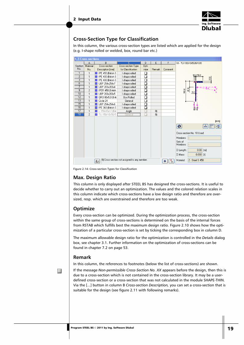
Cross-Section Type for Classification In this column, the various cross-section types are listed which are applied for the design (e.g. I-shape rolled or welded, box, round bar etc.)

Figure 2.14: Cross-section Types for Classification

Max. Design Ratio This column is only displayed after STEEL BS has designed the cross-sections. It is useful to decide whether to carry out an optimization. The values and the colored relation scales in this column indicate which cross-sections have a low design ratio and therefore are over-sized, resp. which are overstrained and therefore are too weak.

Optimize Every cross-section can be optimized. During the optimization process, the cross-section within the same group of cross-sections is determined on the basis of the internal forces from RSTAB which fulfills best the maximum design ratio. Figure 2.10 shows how the opti-mization of a particular cross-section is set by ticking the corresponding box in column D.

The maximum allowable design ratio for the optimization is controlled in the Details dialog box, see chapter 3.1. Further information on the optimization of cross-sections can be found in chapter 7.2 on page 53.

Remark In this column, the references to footnotes (below the list of cross-sections) are shown.

If the message Non-permissible Cross-Section No. XX appears before the design, then this is due to a cross-section which is not contained in the cross-section library. It may be a user-defined cross-section or a cross-section that was not calculated in the module SHAPE-THIN. Via the [...] button in column B Cross-section Description, you can set a cross-section that is suitable for the design (see figure 2.11 with following remarks).

2 Input Data


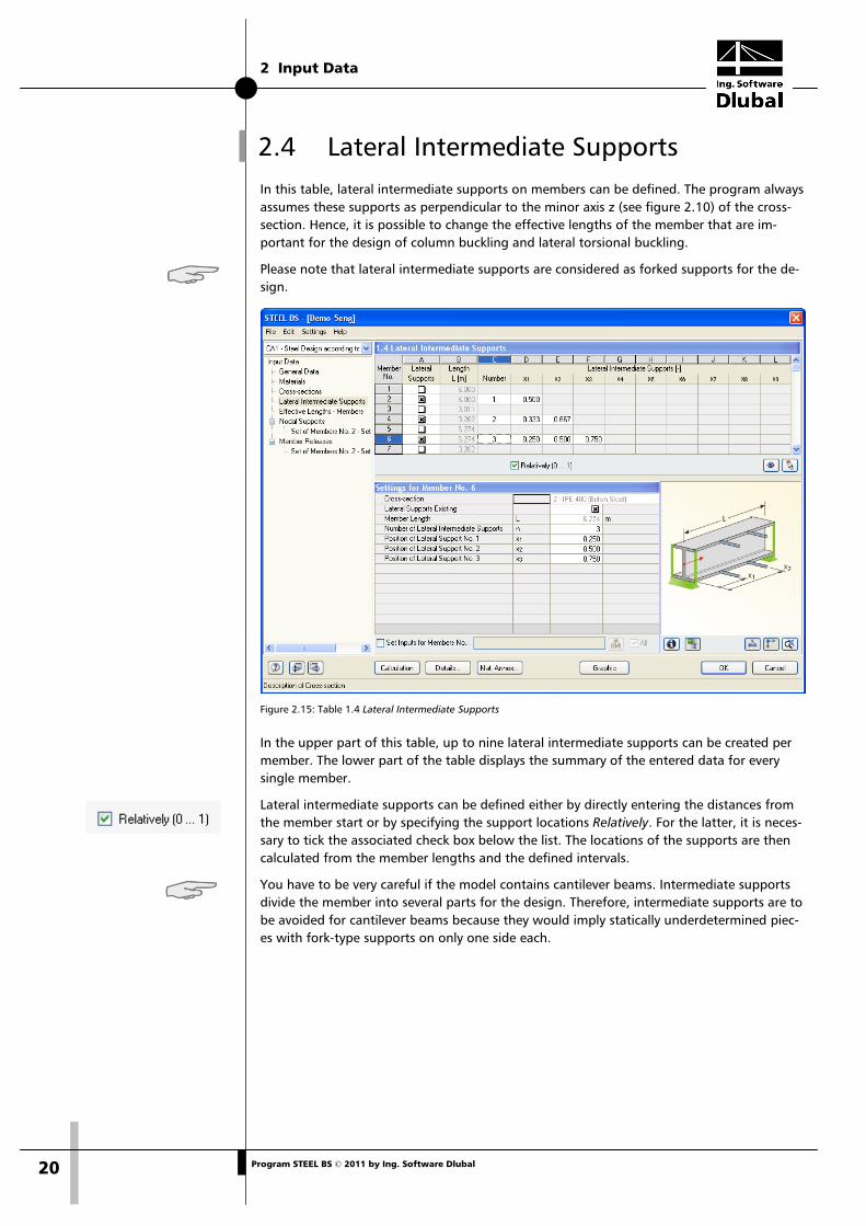
2.4 Lateral Intermediate Supports In this table, lateral intermediate supports on members can be defined. The program always assumes these supports as perpendicular to the minor axis z (see figure 2.10) of the cross-section. Hence, it is possible to change the effective lengths of the member that are im-portant for the design of column buckling and lateral torsional buckling.

Please note that lateral intermediate supports are considered as forked supports for the de-sign.

Figure 2.15: Table 1.4 Lateral Intermediate Supports

In the upper part of this table, up to nine lateral intermediate supports can be created per member. The lower part of the table displays the summary of the entered data for every single member.

Lateral intermediate supports can be defined either by directly entering the distances from the member start or by specifying the support locations Relatively. For the latter, it is neces-sary to tick the associated check box below the list. The locations of the supports are then calculated from the member lengths and the defined intervals.

You have to be very careful if the model contains cantilever beams. Intermediate supports divide the member into several parts for the design. Therefore, intermediate supports are to be avoided for cantilever beams because they would imply statically underdetermined piec-es with fork-type supports on only one side each.

2 Input Data


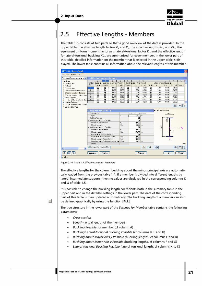
2.5 Effective Lengths - Members The table 1.5 consists of two parts so that a good overview of the data is provided. In the upper table, the effective length factors Ky and Kz, the effective lengths KLy and KLz, the equivalent uniform moment factor mLT, lateral-torsional factor KLT and the effective length for lateral-torsional buckling KLLT are summarized for every member. In the lower part of this table, detailed information on the member that is selected in the upper table is dis-played. The lower table contains all information about the relevant lengths of this member.

Figure 2.16: Table 1.5 Effective Lengths - Members

The effective lengths for the column buckling about the minor principal axis are automati-cally loaded from the previous table 1.4. If a member is divided into different lengths by lateral intermediate supports, then no values are displayed in the corresponding columns D and G of table 1.5.

It is possible to change the buckling length coefficients both in the summary table in the upper part and in the detailed settings in the lower part. The data of the corresponding part of this table is then updated automatically. The buckling length of a member can also be defined graphically by using the function [Pick].

The tree structure in the lower part of the Settings for Member table contains the following parameters:

• Cross-section

• Length (actual length of the member)

• Buckling Possible for member (cf column A)

• Buckling/Lateral-torsional Buckling Possible (cf columns B, E and H)

• Buckling about Mayor Axis y Possible (buckling lengths, cf columns C and D)

• Buckling about Minor Axis z Possible (buckling lengths, cf columns F and G)

• Lateral-torsional Buckling Possible (lateral-torsional length, cf columns H to K)

2 Input Data


It is also possible to modify the Buckling Length Coefficients in the relevant directions and decide whether the buckling design is to be executed. If a buckling length coefficient is changed, the respective effective member length is modified automatically.

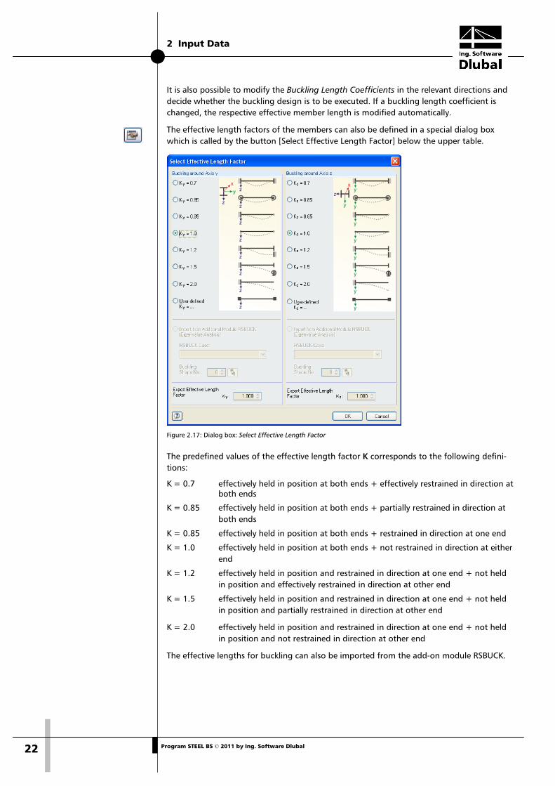
The effective length factors of the members can also be defined in a special dialog box which is called by the button [Select Effective Length Factor] below the upper table.

Figure 2.17: Dialog box: Select Effective Length Factor

The predefined values of the effective length factor K corresponds to the following defini-tions:

K = 0.7 effectively held in position at both ends + effectively restrained in direction at both ends

K = 0.85 effectively held in position at both ends + partially restrained in direction at both ends

K = 0.85 effectively held in position at both ends + restrained in direction at one end

K = 1.0 effectively held in position at both ends + not restrained in direction at either end

K = 1.2 effectively held in position and restrained in direction at one end + not held in position and effectively restrained in direction at other end

K = 1.5 effectively held in position and restrained in direction at one end + not held in position and partially restrained in direction at other end

K = 2.0 effectively held in position and restrained in direction at one end + not held in position and not restrained in direction at other end

The effective lengths for buckling can also be imported from the add-on module RSBUCK.

2 Input Data


Buckling Possible For the stability design of the buckling and lateral-torsional buckling, it is necessary for the member to transfer compression forces. Members that cannot transfer compression forces due to their definition (e.g. tension members, elastic foundations, rigid couplings) are a pri-ori excluded from the stability design in STEEL BS. In such a case, a corresponding comment is displayed in the column Comment for this member.

The column Buckling Possible makes it possible to classify specific members as compression members or, alternatively, to exclude them from the design. Hence, the check boxes in col-umn A and also in table Settings for Member No. control whether the input options for the buckling length parameters are accessible for a member.

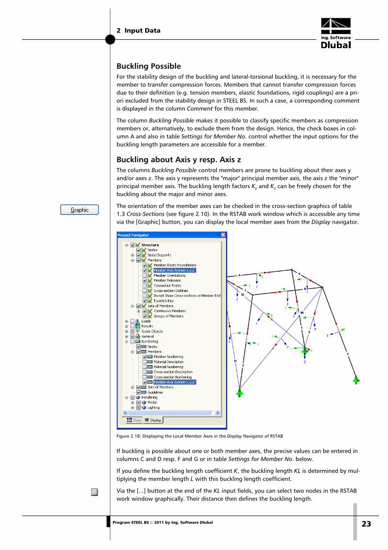
Buckling about Axis y resp. Axis z The columns Buckling Possible control members are prone to buckling about their axes y and/or axes z. The axis y represents the "major" principal member axis, the axis z the "minor" principal member axis. The buckling length factors Ky and Kz can be freely chosen for the buckling about the major and minor axes.

The orientation of the member axes can be checked in the cross-section graphics of table 1.3 Cross-Sections (see figure 2.10). In the RSTAB work window which is accessible any time via the [Graphic] button, you can display the local member axes from the Display navigator.

Figure 2.18: Displaying the Local Member Axes in the Display Navigator of RSTAB

If buckling is possible about one or both member axes, the precise values can be entered in columns C and D resp. F and G or in table Settings for Member No. below.

If you define the buckling length coefficient K, the buckling length KL is determined by mul-tiplying the member length L with this buckling length coefficient.

Via the [...] button at the end of the KL input fields, you can select two nodes in the RSTAB work window graphically. Their distance then defines the buckling length.

2 Input Data


Lateral-Torsional Buckling Column H controls whether a lateral torsional buckling design is to be carried out.

In column I, three options are available for defining the equivalent uniform moment factor mLT. The default value is 1.0. The factor can also be determined by the program according to table 18 [1] or entered manually.

Column J enables you to modify the lateral-torsional buckling coefficient KLT which has an influence on the calculation of the lateral-torsional buckling length. The value of KLT is pre-set to 1.0.

If the lateral-torsional buckling coefficient is changed, the respective lateral-torsional buck-ling length KLLT is modified automatically. The values in column K depend on the settings in table 1.4 Lateral Intermediate Supports. It is also possible to enter values of KLLT manually.

Comment In the last column the user can write down his own remarks at every member, e.g. to ex-plain more closely the specific lengths of a member.

The check box Set Inputs for Members No. is located beneath the tree-structure lower table. If you tick this box, the data entered consequently will become valid for specific resp. All members. You can select the members graphically by using the function [Pick] or enter their numbers manually. This option is useful when you want to assign the same boundary con-ditions to several members. Please notice that this function must be activated prior to data entering. If you define the data and choose this option later, the data is not re-assigned.

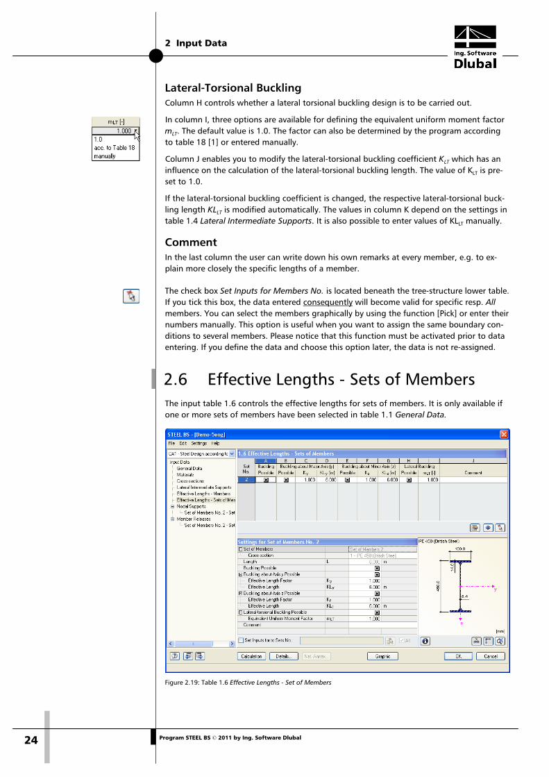
2.6 Effective Lengths - Sets of Members The input table 1.6 controls the effective lengths for sets of members. It is only available if one or more sets of members have been selected in table 1.1 General Data.

Figure 2.19: Table 1.6 Effective Lengths - Set of Members

2 Input Data


This table is very similar to the previous table 1.5. With regard to the effective lengths for buckling about the major and minor axes of the cross-sections, it is identical to table 1.5.

There are differences, however, as far as the parameters for torsional and lateral-torsional buckling are concerned. These are defined by means of specific boundary conditions in ta-ble 1.8 (see chapter 2.8).

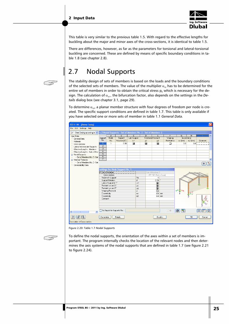
2.7 Nodal Supports The stability design of sets of members is based on the loads and the boundary conditions of the selected sets of members. The value of the multiplier αcr has to be determined for the entire set of members in order to obtain the critical stress pE which is necessary for the de-sign. The calculation of αcr , the bifurcation factor, also depends on the settings in the De-tails dialog box (see chapter 3.1, page 29).

To determine αcr, a planar member structure with four degrees of freedom per node is cre-ated. The specific support conditions are defined in table 1.7. This table is only available if you have selected one or more sets of member in table 1.1 General Data.

Figure 2.20: Table 1.7 Nodal Supports

To define the nodal supports, the orientation of the axes within a set of members is im-portant. The program internally checks the location of the relevant nodes and then deter-mines the axis systems of the nodal supports that are defined in table 1.7 (see figure 2.21 to figure 2.24).

2 Input Data


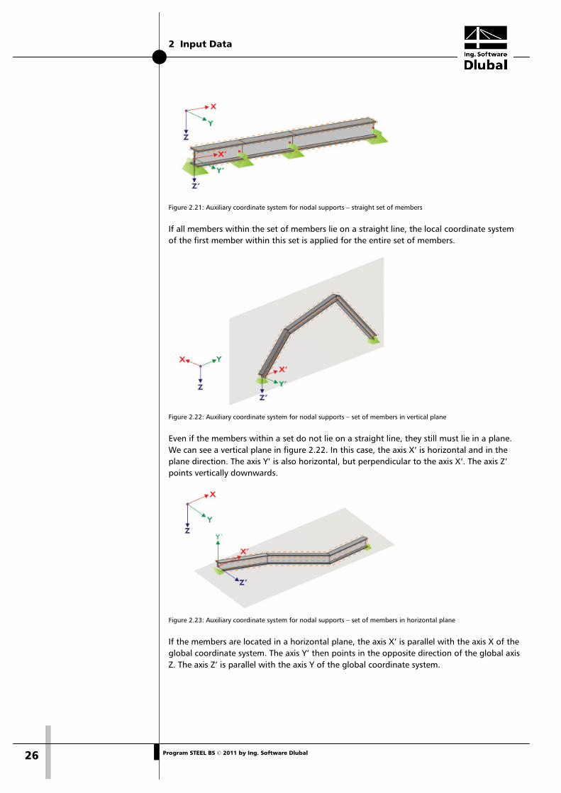
Figure 2.21: Auxiliary coordinate system for nodal supports – straight set of members

If all members within the set of members lie on a straight line, the local coordinate system of the first member within this set is applied for the entire set of members.

Figure 2.22: Auxiliary coordinate system for nodal supports – set of members in vertical plane

Even if the members within a set do not lie on a straight line, they still must lie in a plane. We can see a vertical plane in figure 2.22. In this case, the axis X’ is horizontal and in the plane direction. The axis Y’ is also horizontal, but perpendicular to the axis X’. The axis Z’ points vertically downwards.

Figure 2.23: Auxiliary coordinate system for nodal supports – set of members in horizontal plane

If the members are located in a horizontal plane, the axis X’ is parallel with the axis X of the global coordinate system. The axis Y’ then points in the opposite direction of the global axis Z. The axis Z’ is parallel with the axis Y of the global coordinate system.

2 Input Data


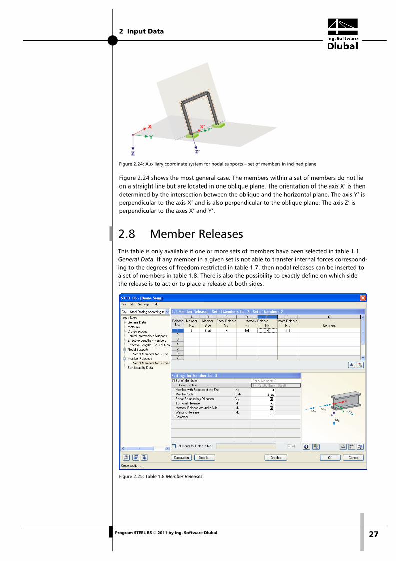
Figure 2.24: Auxiliary coordinate system for nodal supports – set of members in inclined plane

Figure 2.24 shows the most general case. The members within a set of members do not lie on a straight line but are located in one oblique plane. The orientation of the axis X’ is then determined by the intersection between the oblique and the horizontal plane. The axis Y’ is perpendicular to the axis X’ and is also perpendicular to the oblique plane. The axis Z’ is perpendicular to the axes X’ and Y’.

2.8 Member Releases This table is only available if one or more sets of members have been selected in table 1.1 General Data. If any member in a given set is not able to transfer internal forces correspond-ing to the degrees of freedom restricted in table 1.7, then nodal releases can be inserted to a set of members in table 1.8. There is also the possibility to exactly define on which side the release is to act or to place a release at both sides.

Figure 2.25: Table 1.8 Member Releases

2 Input Data


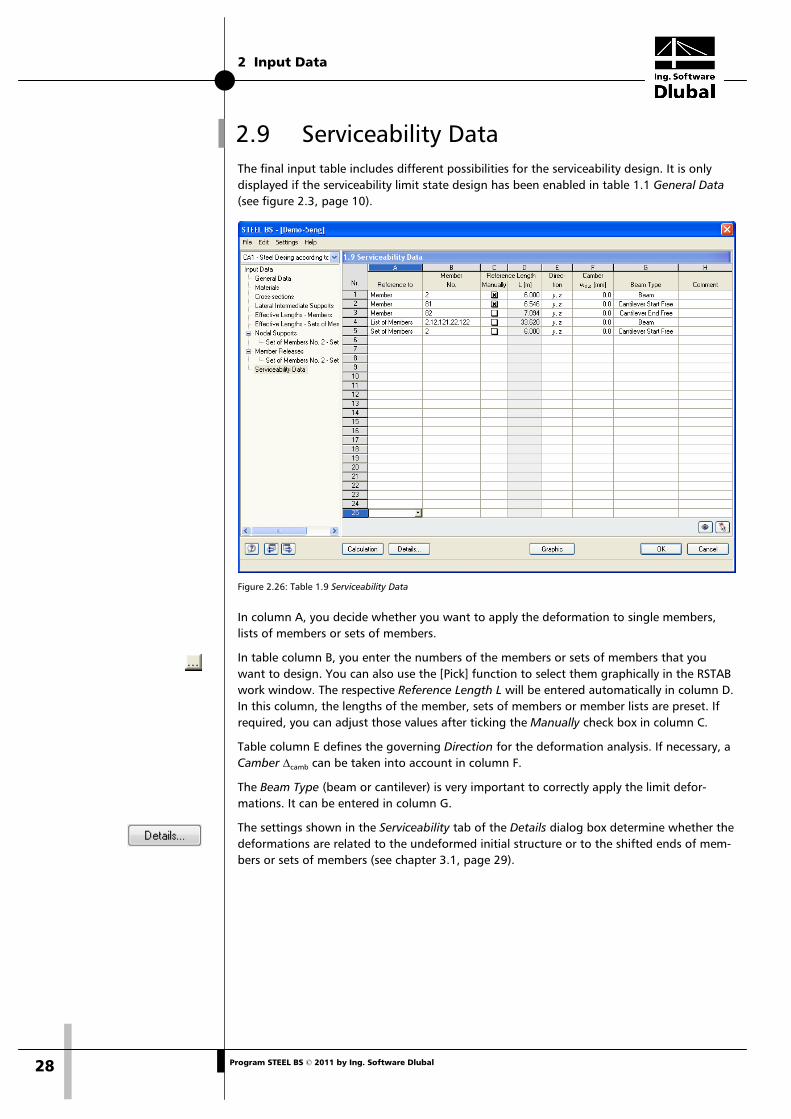
2.9 Serviceability Data The final input table includes different possibilities for the serviceability design. It is only displayed if the serviceability limit state design has been enabled in table 1.1 General Data (see figure 2.3, page 10).

Figure 2.26: Table 1.9 Serviceability Data

In column A, you decide whether you want to apply the deformation to single members, lists of members or sets of members.

In table column B, you enter the numbers of the members or sets of members that you want to design. You can also use the [Pick] function to select them graphically in the RSTAB work window. The respective Reference Length L will be entered automatically in column D. In this column, the lengths of the member, sets of members or member lists are preset. If required, you can adjust those values after ticking the Manually check box in column C.

Table column E defines the governing Direction for the deformation analysis. If necessary, a Camber ∆camb can be taken into account in column F.

The Beam Type (beam or cantilever) is very important to correctly apply the limit defor-mations. It can be entered in column G.

The settings shown in the Serviceability tab of the Details dialog box determine whether the deformations are related to the undeformed initial structure or to the shifted ends of mem-bers or sets of members (see chapter 3.1, page 29).

3 Calculation


3. Calculation

3.1 Details A particular design is carried out with the internal forces calculated in the RSTAB program. Before the [Calculation], you should check the detailed setting for the design. Open the ap-propriate dialog box from every input or output table by clicking the [Details] button.

The Details dialog box consists of four tabs: Ultimate Limit State, Stability, Serviceability and Other.

Ultimate Limit State Options STEEL BS carries out a plastic design for cross-sections of classes 1 or 2. If needed, the Elas-tic design can be activated for those cross-section classes in the Ultimate Limit State tab.

Stability

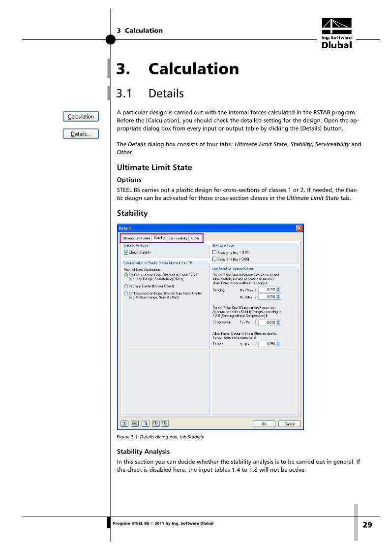
Figure 3.1: Details dialog box, tab Stability

Stability Analysis In this section you can decide whether the stability analysis is to be carried out in general. If the check is disabled here, the input tables 1.4 to 1.8 will not be active.

3 Calculation


Determination of Elastic Critical Moment for LTB Usually, loads act on members. Then their application point has to be specified because this can have stabilizing or destabilizing effects, subject to the eccentricity. The Point of Applied Load can be set globally for all loads.

The elastic critical stress pE is calculated automatically for sets of members.

Structure Type The structure type can be either Non-sway or Sway, which affects the calculation of my and mz. For a sway-type structure, the values of my and mz are assumed as 0.85.

Limit Load for Special Cases It is possible to neglect small stresses due to bending compressive forces and torsion and, thus, allow a simplified design which eliminates negligible internal forces. In this dialog sec-tion, the limits of these internal forces or stresses can be entered. Those are defined as the ratios between existing internal forces or stresses and the corresponding resistances of each cross-section.

If one of those limits is exceeded, a comment will be given in the results table. There will be no stability design. Nevertheless, the design of the cross-section itself is carried out. Please not that those limit values are not part of the British Standard. If you change the limits, it will be in your own area of responsibility.

Serviceability Serviceability (Deflections) In this section, it is possible to check or change the allowable deflections for the serviceabil-ity limit state design. The default values are L/360 for beams and L/180 for cantilevers.

The two selection fields below control whether the Deformation is to be related to the un-deformed model or to an imaginary connecting line between the shifted start and end nodes of the member resp. set of members within the deformed structure.

Other Cross-section Optimization Cross-sections can be optimized if the Optimize option is chosen in table 1.3 Cross-Sections. (see figure 2.10, page 16). The dialog box Details enables you to set the maximum allowa-ble design ratio as a limit for the optimization process.

Check of Member Slendernesses It is possible to set user-defined slenderness ratios KL/r for members with tension resp. compression or flexure. These maximum values are compared with the actual member slen-dernesses in table 3.3 which is available after the calculation (see chapter 4.8).

Display Results Tables In this section, the results tables can be specified which are to be displayed, inclusive of a parts list. The results tables are described individually in chapter 4.

3 Calculation


3.2 Start Calculation In all input tables of STEEL BS, you can start the design via the [Calculation] button.

At first, STEEL BS searches for the results of the selected load cases, load groups and com-binations. If they are not found, the calculation of the governing internal forces in RSTAB is started. The calculation parameters of RSTAB are used for this analysis.

If cross-sections are to be optimized (see chapter 7.2, page 53), the required sections are calculated and relevant types of design are carried out.

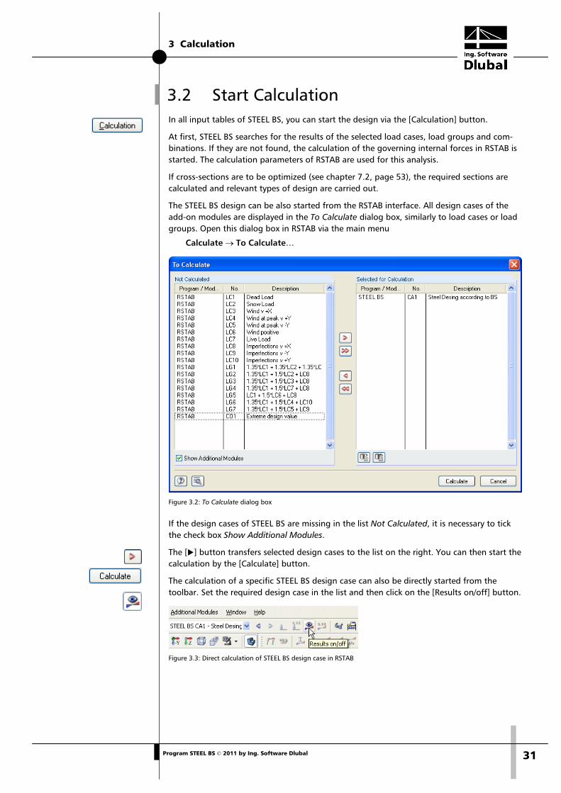
The STEEL BS design can be also started from the RSTAB interface. All design cases of the add-on modules are displayed in the To Calculate dialog box, similarly to load cases or load groups. Open this dialog box in RSTAB via the main menu

Calculate → To Calculate…

Figure 3.2: To Calculate dialog box

If the design cases of STEEL BS are missing in the list Not Calculated, it is necessary to tick the check box Show Additional Modules.

The [] button transfers selected design cases to the list on the right. You can then start the calculation by the [Calculate] button.

The calculation of a specific STEEL BS design case can also be directly started from the toolbar. Set the required design case in the list and then click on the [Results on/off] button.

Figure 3.3: Direct calculation of STEEL BS design case in RSTAB

3 Calculation


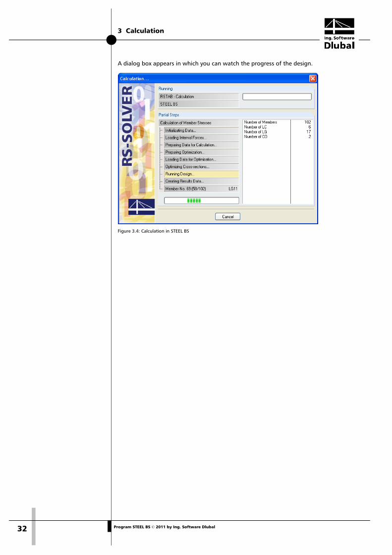
A dialog box appears in which you can watch the progress of the design.

Figure 3.4: Calculation in STEEL BS

4 Results


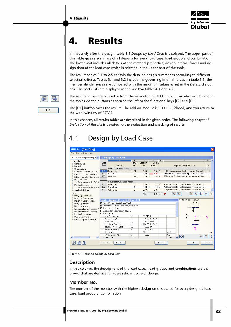
4. Results Immediately after the design, table 2.1 Design by Load Case is displayed. The upper part of this table gives a summary of all designs for every load case, load group and combination. The lower part includes all details of the material properties, design internal forces and de-sign data of the load case which is selected in the upper part of the table.

The results tables 2.1 to 2.5 contain the detailed design summaries according to different selection criteria. Tables 3.1 and 3.2 include the governing internal forces. In table 3.3, the member slendernesses are compared with the maximum values as set in the Details dialog box. The parts lists are displayed in the last two tables 4.1 and 4.2.

The results tables are accessible from the navigator in STEEL BS. You can also switch among the tables via the buttons as seen to the left or the functional keys [F2] and [F3].

The [OK] button saves the results. The add-on module is STEEL BS closed, and you return to the work window of RSTAB.

In this chapter, all results tables are described in the given order. The following chapter 5 Evaluation of Results is devoted to the evaluation and checking of results.

4.1 Design by Load Case

Figure 4.1: Table 2.1 Design by Load Case

Description In this column, the descriptions of the load cases, load groups and combinations are dis-played that are decisive for every relevant type of design.

Member No. The number of the member with the highest design ratio is stated for every designed load case, load group or combination.

4 Results


Location x The location x on the member where the maximum stress ratio occurs is displayed in this column. The following locations x on the member are taken into account:

• Start and end nodes

• Internal nodes according to potential user-defined member division

• Member division according to specification for member results (Options tab of RSTAB dialog box Calculation Parameters)

• Extreme values of internal forces

Design Ratio For every design type and for every load case, load group or combination, the design quo-tients according to the standard are displayed in this column.

The colored scales represent the design ratios due to the individual load cases.

Design according to Formula In this column, the equations that were followed in the design are listed.

DS The final column contains information about the respective design-relevant Design Situa-tion: ULS (ultimate limit state) or one of the three design situations for serviceability (CH, FR, QP) according to the specification in table 1.1 General Data (see figure 2.3, page 10).

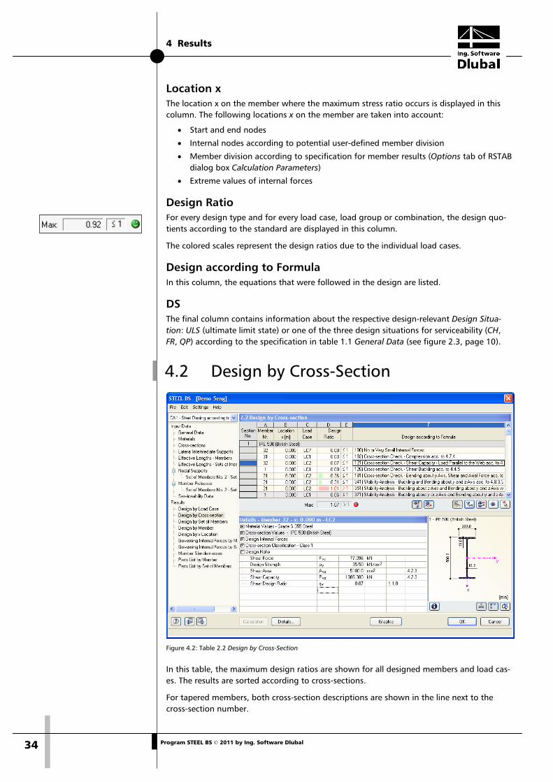
4.2 Design by Cross-Section

Figure 4.2: Table 2.2 Design by Cross-Section

In this table, the maximum design ratios are shown for all designed members and load cas-es. The results are sorted according to cross-sections.

For tapered members, both cross-section descriptions are shown in the line next to the cross-section number.

4 Results


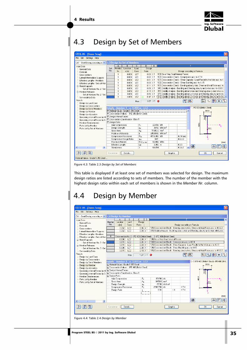
4.3 Design by Set of Members

Figure 4.3: Table 2.3 Design by Set of Members

This table is displayed if at least one set of members was selected for design. The maximum design ratios are listed according to sets of members. The number of the member with the highest design ratio within each set of members is shown in the Member Nr. column.

4.4 Design by Member

Figure 4.4: Table 2.4 Design by Member

4 Results


In this table, the maximum design ratios are arranged according to member numbers.

The description of the individual columns can be found in chapter 4.1 on page 33.

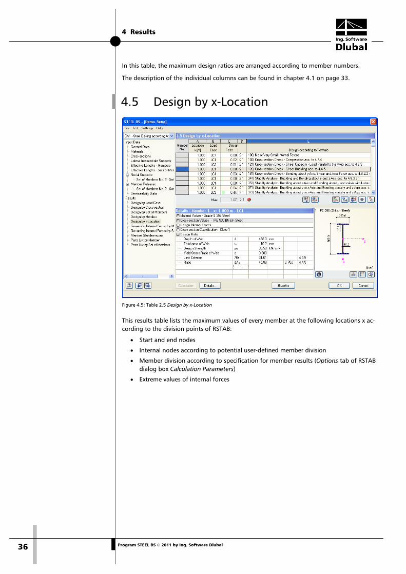
4.5 Design by x-Location

Figure 4.5: Table 2.5 Design by x-Location

This results table lists the maximum values of every member at the following locations x ac-cording to the division points of RSTAB:

• Start and end nodes

• Internal nodes according to potential user-defined member division

• Member division according to specification for member results (Options tab of RSTAB dialog box Calculation Parameters)

• Extreme values of internal forces

4 Results


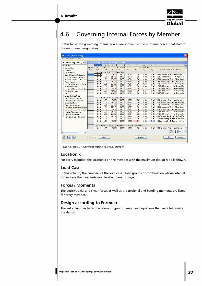
4.6 Governing Internal Forces by Member In this table, the governing internal forces are shown, i.e. those internal forces that lead to the maximum design ratios.

Figure 4.6: Table 3.1 Governing Internal Forces by Member

Location x For every member, the location x on the member with the maximum design ratio is shown.

Load Case In this column, the numbers of the load cases, load groups or combination whose internal forces have the most unfavorable effects are displayed.

Forces / Moments The decisive axial and shear forces as well as the torsional and bending moments are listed for every member.

Design according to Formula The last column includes the relevant types of design and equations that were followed in the design.

4 Results


4.7 Governing Internal Forces by Set of Members

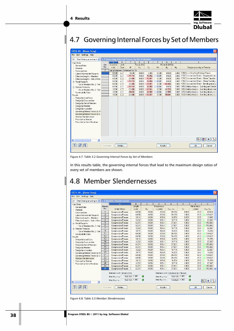
Figure 4.7: Table 3.2 Governing Internal Forces by Set of Members

In this results table, the governing internal forces that lead to the maximum design ratios of every set of members are shown.

4.8 Member Slendernesses

Figure 4.8: Table 3.3 Member Slendernesses

4 Results


In table 3.3, the effective slenderness ratios of all designed members are compared with the maximum values that were set in the Details dialog box (see chapter 3.1). These ratios are listed with respect to the major and minor principal axes. This table provides information on the maximum effective slenderness ratios only, it does not give any design results.

Members of the types "Tension" or "Cable" are excluded from this table.

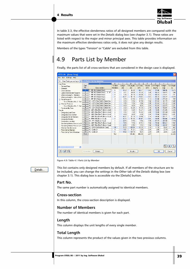
4.9 Parts List by Member Finally, the parts list of all cross-sections that are considered in the design case is displayed.

Figure 4.9: Table 4.1 Parts List by Member

This list contains only designed members by default. If all members of the structure are to be included, you can change the settings in the Other tab of the Details dialog box (see chapter 3.1). This dialog box is accessible via the [Details] button.

Part No. The same part number is automatically assigned to identical members.

Cross-section In this column, the cross-section description is displayed.

Number of Members The number of identical members is given for each part.

Length This column displays the unit lengths of every single member.

Total Length This column represents the product of the values given in the two previous columns.

4 Results


Surface Area The surface area which is related to the total length of the relevant part is calculated on the basis of the value ASurf of each cross-section. You can check on this value by clicking on the [Info about Current Cross-Section] button in tables 1.3 or 2.1 to 2.5.

Volume The volume of every part is calculated from the surface area and the total length.

Unit Weight The Unit Weight of the cross-section represents the weight per length of 1 m. For tapered cross-sections, the unit weight is calculated as the mean value of both cross-sections.

Weight The value in this column is calculated as the product of values in the columns C and G.

Total Weight The total weight of each part is displayed in the last column.

Sum The sums of the values listed in columns B, D, E, F and I are given in the final row of the list. The cell Total Weight shows the total required mass of steel.

4.10 Parts List by Set of Members

Figure 4.10: Table 4.2 Parts List by Set of Members

The last table in STEEL BS is presented when at least one set of members was selected for the design. The advantage of this table is that a parts list is given for the various groups of elements (e.g. for a beam).

The table columns are described in chapter 4.9. If there are different cross-sections within the set of members, the mean values of surface area, volume and unit weight are listed.

5 Evaluation of Results


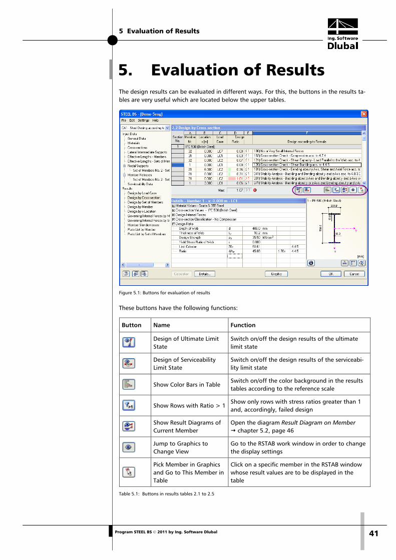
5. Evaluation of Results The design results can be evaluated in different ways. For this, the buttons in the results ta-bles are very useful which are located below the upper tables.

Figure 5.1: Buttons for evaluation of results

These buttons have the following functions:

Button Name Function

Design of Ultimate Limit State

Switch on/off the design results of the ultimate limit state

Design of Serviceability Limit State

Switch on/off the design results of the serviceabi-lity limit state

Show Color Bars in Table Switch on/off the color background in the results tables according to the reference scale

Show Rows with Ratio > 1 Show only rows with stress ratios greater than 1 and, accordingly, failed design

Show Result Diagrams of Current Member

Open the diagram Result Diagram on Member chapter 5.2, page 46

Jump to Graphics to Change View

Go to the RSTAB work window in order to change the display settings

Pick Member in Graphics and Go to This Member in Table

Click on a specific member in the RSTAB window whose result values are to be displayed in the table

Table 5.1: Buttons in results tables 2.1 to 2.5



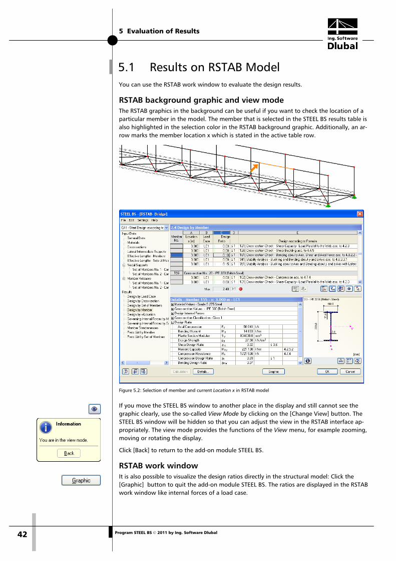
5.1 Results on RSTAB Model You can use the RSTAB work window to evaluate the design results.

RSTAB background graphic and view mode The RSTAB graphics in the background can be useful if you want to check the location of a particular member in the model. The member that is selected in the STEEL BS results table is also highlighted in the selection color in the RSTAB background graphic. Additionally, an ar-row marks the member location x which is stated in the active table row.

Figure 5.2: Selection of member and current Location x in RSTAB model

If you move the STEEL BS window to another place in the display and still cannot see the graphic clearly, use the so-called View Mode by clicking on the [Change View] button. The STEEL BS window will be hidden so that you can adjust the view in the RSTAB interface ap-propriately. The view mode provides the functions of the View menu, for example zooming, moving or rotating the display.

Click [Back] to return to the add-on module STEEL BS.

RSTAB work window It is also possible to visualize the design ratios directly in the structural model: Click the [Graphic] button to quit the add-on module STEEL BS. The ratios are displayed in the RSTAB work window like internal forces of a load case.



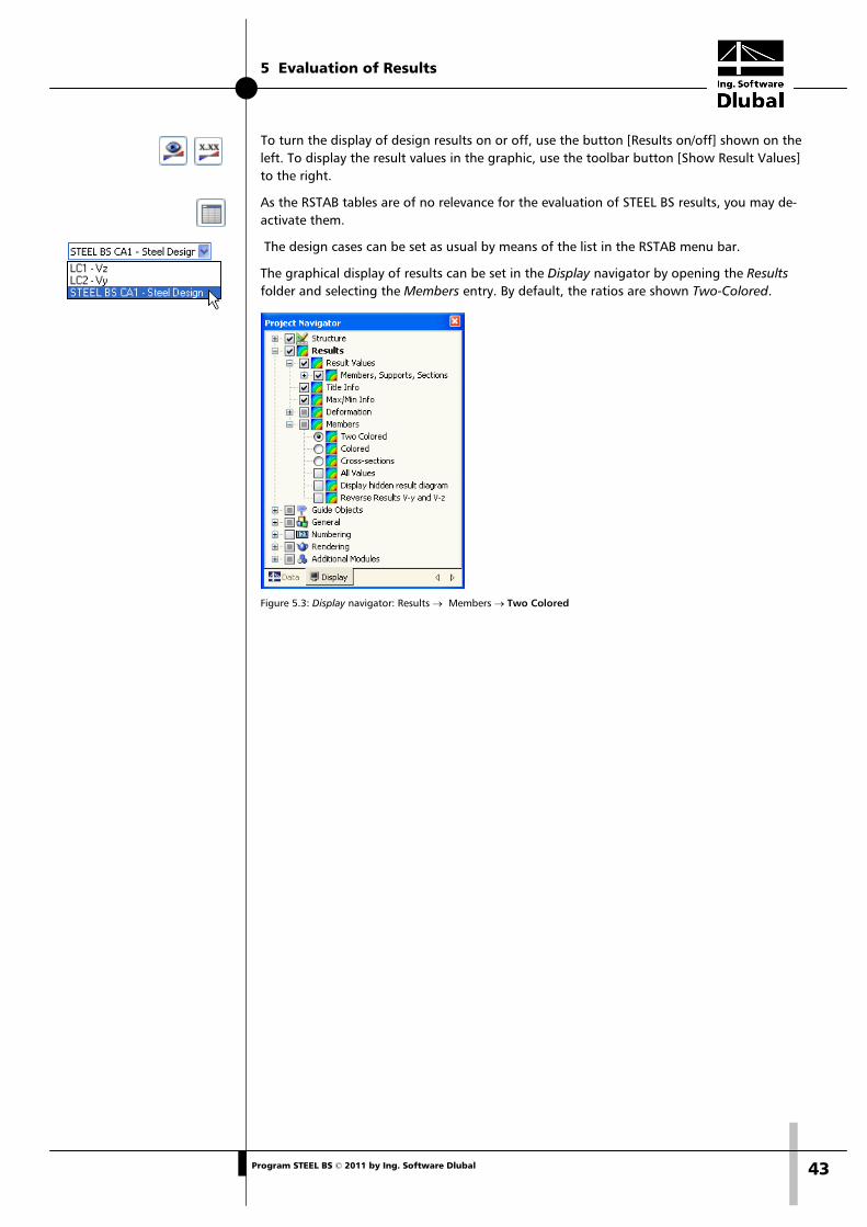
To turn the display of design results on or off, use the button [Results on/off] shown on the left. To display the result values in the graphic, use the toolbar button [Show Result Values] to the right.

As the RSTAB tables are of no relevance for the evaluation of STEEL BS results, you may de-activate them.

The design cases can be set as usual by means of the list in the RSTAB menu bar.

The graphical display of results can be set in the Display navigator by opening the Results folder and selecting the Members entry. By default, the ratios are shown Two-Colored.

Figure 5.3: Display navigator: Results → Members → Two Colored



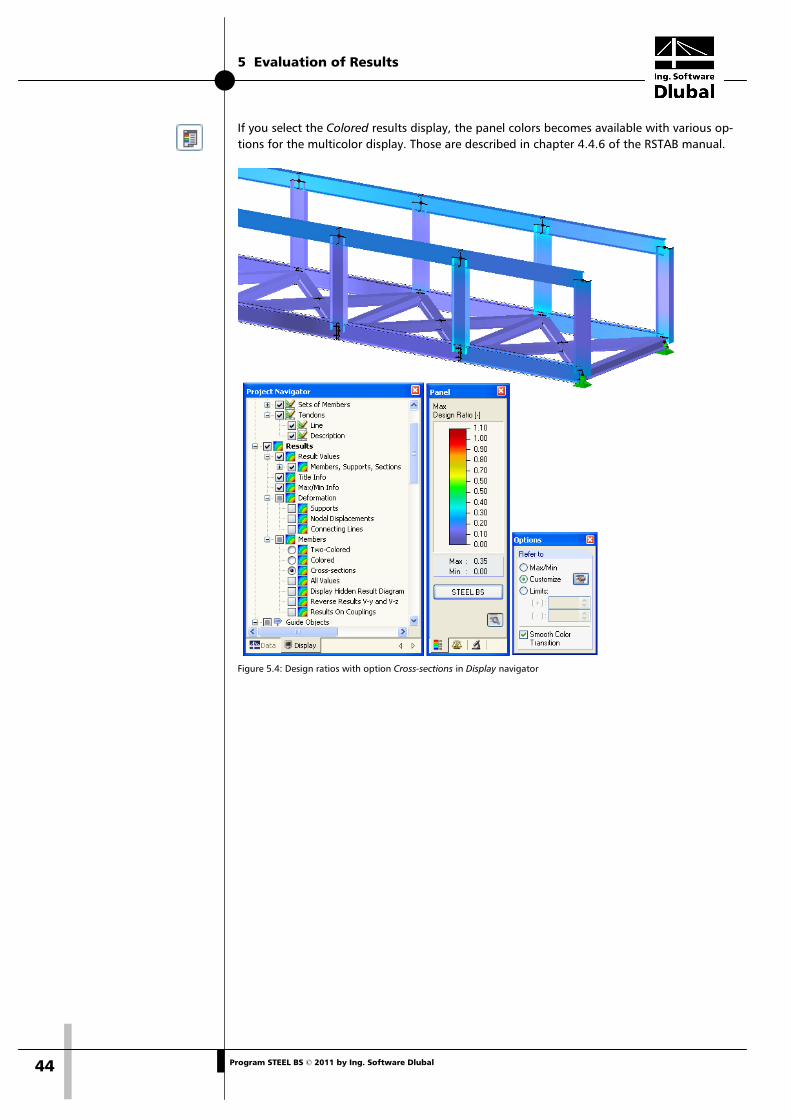
If you select the Colored results display, the panel colors becomes available with various op-tions for the multicolor display. Those are described in chapter 4.4.6 of the RSTAB manual.

Figure 5.4: Design ratios with option Cross-sections in Display navigator



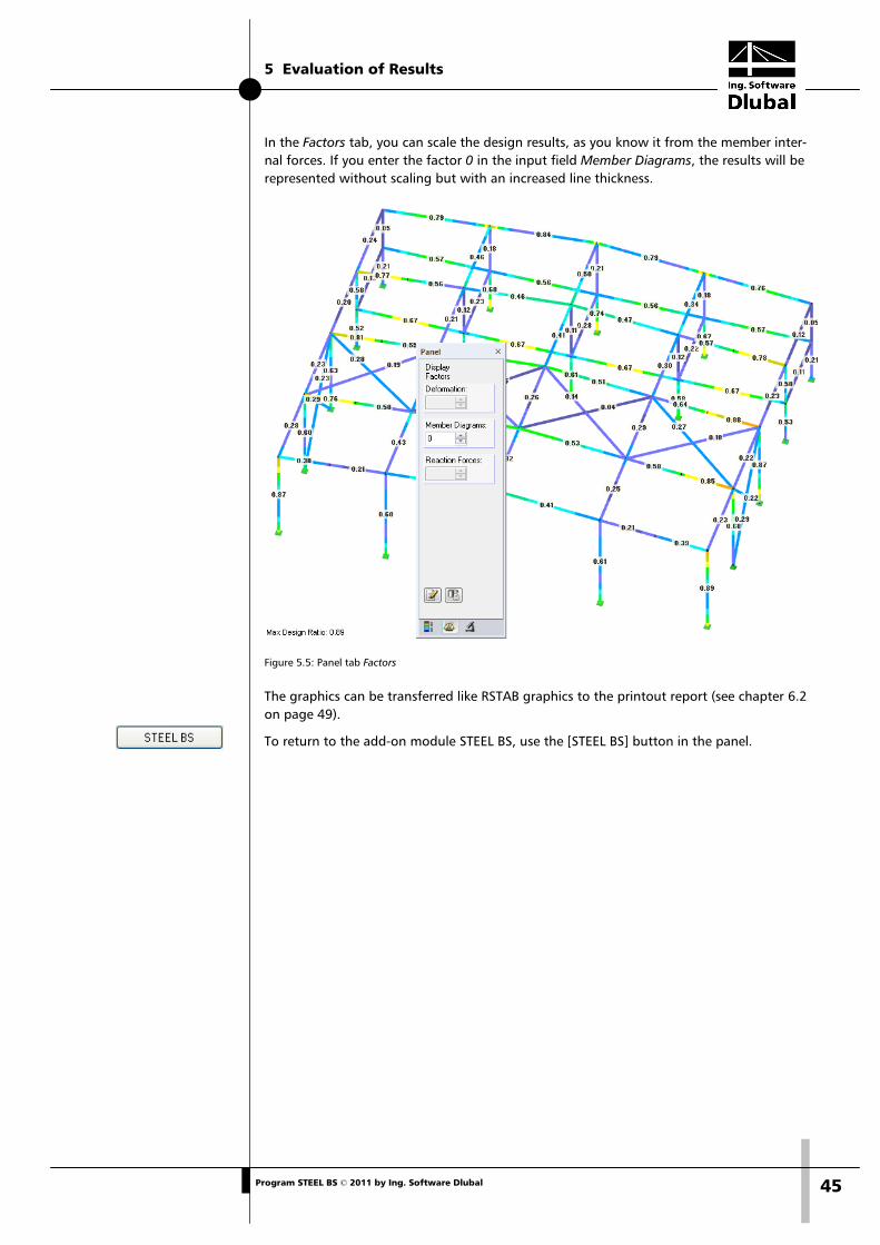
In the Factors tab, you can scale the design results, as you know it from the member inter-nal forces. If you enter the factor 0 in the input field Member Diagrams, the results will be represented without scaling but with an increased line thickness.

Figure 5.5: Panel tab Factors

The graphics can be transferred like RSTAB graphics to the printout report (see chapter 6.2 on page 49).

To return to the add-on module STEEL BS, use the [STEEL BS] button in the panel.



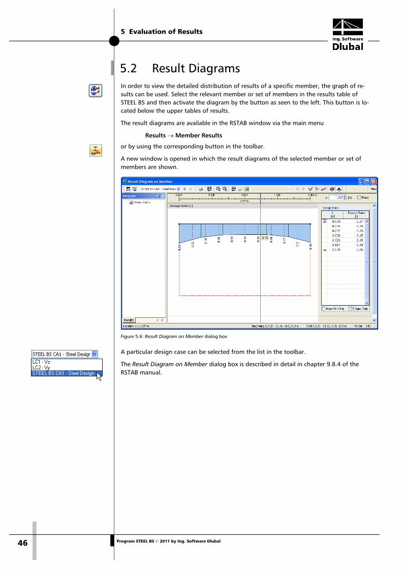
5.2 Result Diagrams In order to view the detailed distribution of results of a specific member, the graph of re-sults can be used. Select the relevant member or set of members in the results table of STEEL BS and then activate the diagram by the button as seen to the left. This button is lo-cated below the upper tables of results.

The result diagrams are available in the RSTAB window via the main menu

Results → Member Results

or by using the corresponding button in the toolbar.

A new window is opened in which the result diagrams of the selected member or set of members are shown.

Figure 5.6: Result Diagram on Member dialog box

A particular design case can be selected from the list in the toolbar.

The Result Diagram on Member dialog box is described in detail in chapter 9.8.4 of the RSTAB manual.



5.3 Filter Results The structure of the STEEL BS tables makes it already possible to select the results according to certain criteria. Additionally, you can use the filter functions as described in the RSTAB manual to graphically evaluate the STEEL BS results.

Firstly, you can use already defined partial views (cf RSTAB manual, chapter 9.8.6) that group certain objects in a favorable way.

Secondly, you can set the stress ratios as criteria for filtering the results in the RSTAB work window. For this, the so-called control panel is to be displayed. If it is not visible, you can switch it on in the main menu

View → Control panel

or by clicking on the corresponding button in the Results toolbar.

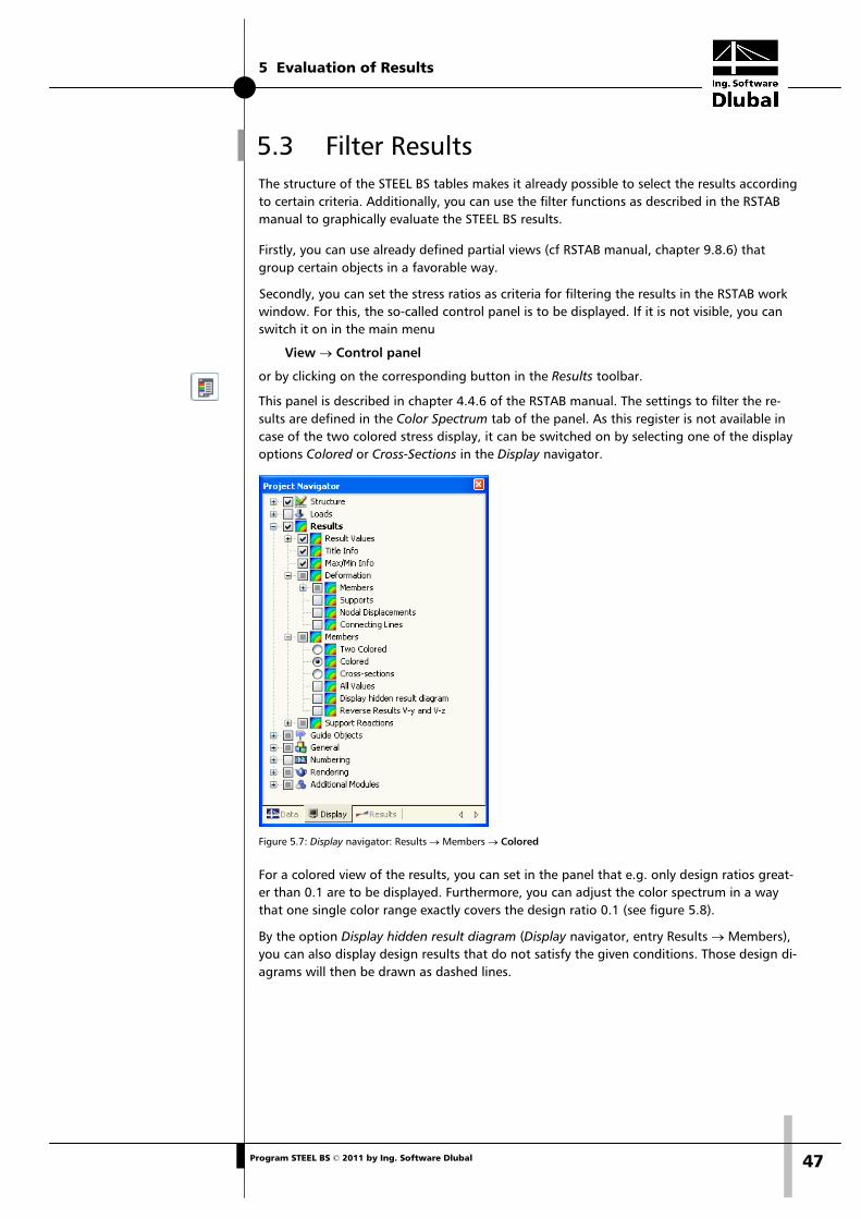
This panel is described in chapter 4.4.6 of the RSTAB manual. The settings to filter the re-sults are defined in the Color Spectrum tab of the panel. As this register is not available in case of the two colored stress display, it can be switched on by selecting one of the display options Colored or Cross-Sections in the Display navigator.

Figure 5.7: Display navigator: Results → Members → Colored

For a colored view of the results, you can set in the panel that e.g. only design ratios great-er than 0.1 are to be displayed. Furthermore, you can adjust the color spectrum in a way that one single color range exactly covers the design ratio 0.1 (see figure 5.8).

By the option Display hidden result diagram (Display navigator, entry Results → Members), you can also display design results that do not satisfy the given conditions. Those design di-agrams will then be drawn as dashed lines.



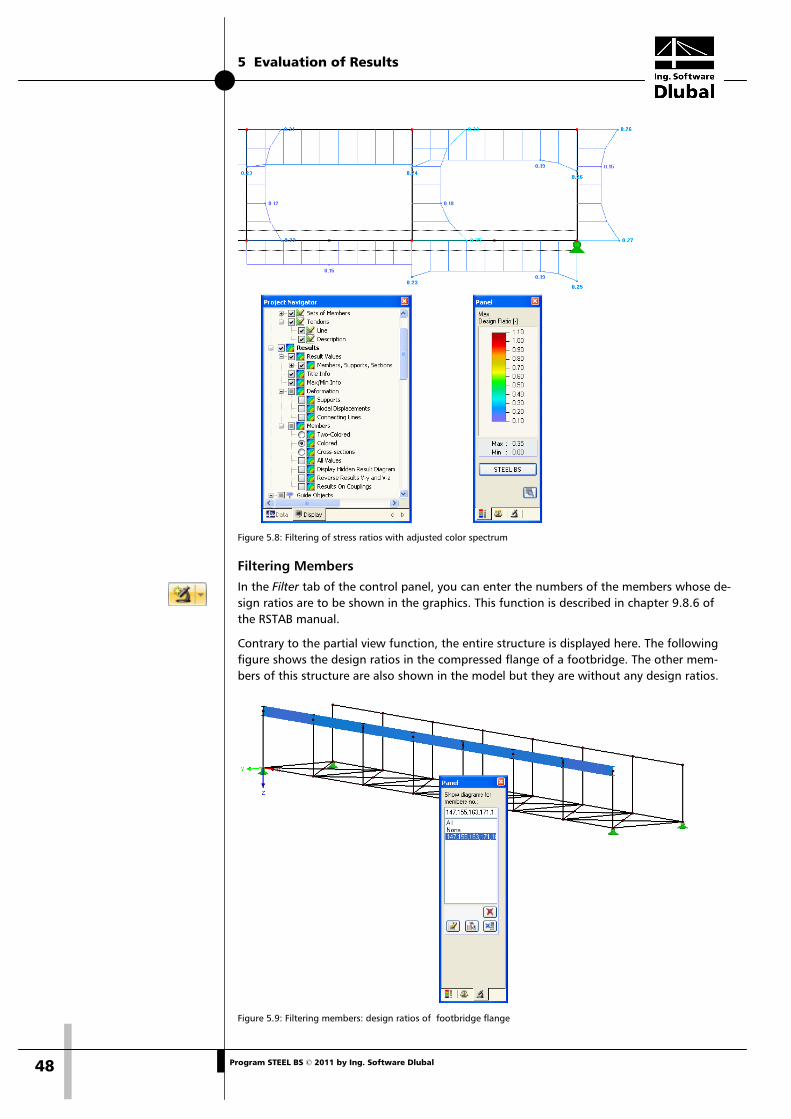
Figure 5.8: Filtering of stress ratios with adjusted color spectrum

Filtering Members In the Filter tab of the control panel, you can enter the numbers of the members whose de-sign ratios are to be shown in the graphics. This function is described in chapter 9.8.6 of the RSTAB manual.

Contrary to the partial view function, the entire structure is displayed here. The following figure shows the design ratios in the compressed flange of a footbridge. The other mem-bers of this structure are also shown in the model but they are without any design ratios.

Figure 5.9: Filtering members: design ratios of footbridge flange

6 Printout


6. Printout

6.1 Printout Report For the design results of STEEL BS, a printout report can be created to which you can add graphics and comments. In this printout report, it is also possible to select the results tables of STEEL BS that are to be printed.

The printout report is described in detail in the manual of the RSTAB program. In particular, chapter 10.1.3.4 Selecting Data of Add-on Modules on page 227 is important. It deals with the selection of input and output data in all add-on modules.

For complex structures with a high number of design cases, it is recommended to split the data into several small printout reports which allows for a clearly-arranged printout and a faster work.

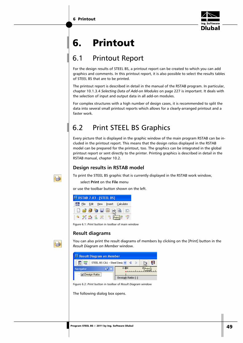
6.2 Print STEEL BS Graphics Every picture that is displayed in the graphic window of the main program RSTAB can be in-cluded in the printout report. This means that the design ratios displayed in the RSTAB model can be prepared for the printout, too. The graphics can be integrated in the global printout report or sent directly to the printer. Printing graphics is described in detail in the RSTAB manual, chapter 10.2.

Design results in RSTAB model To print the STEEL BS graphic that is currently displayed in the RSTAB work window,

select Print on the File menu

or use the toolbar button shown on the left.

Figure 6.1: Print button in toolbar of main window

Result diagrams You can also print the result diagrams of members by clicking on the [Print] button in the Result Diagram on Member window.

Figure 6.2: Print button in toolbar of Result Diagram window

The following dialog box opens.

6 Printout


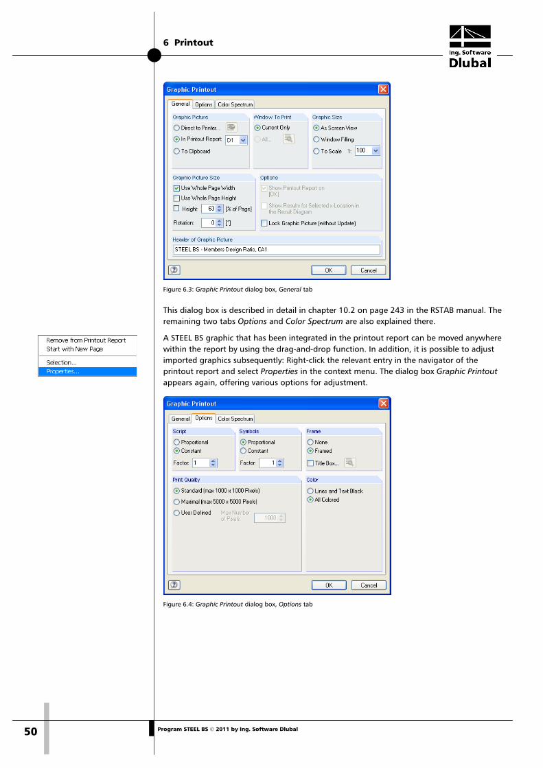
Figure 6.3: Graphic Printout dialog box, General tab

This dialog box is described in detail in chapter 10.2 on page 243 in the RSTAB manual. The remaining two tabs Options and Color Spectrum are also explained there.

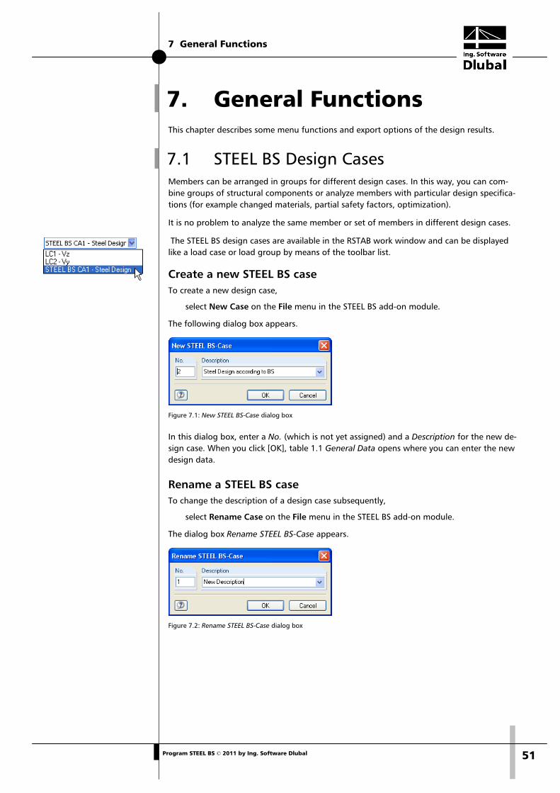
A STEEL BS graphic that has been integrated in the printout report can be moved anywhere within the report by using the drag-and-drop function. In addition, it is possible to adjust imported graphics subsequently: Right-click the relevant entry in the navigator of the printout report and select Properties in the context menu. The dialog box Graphic Printout appears again, offering various options for adjustment.

Figure 6.4: Graphic Printout dialog box, Options tab

7 General Functions


7. General Functions This chapter describes some menu functions and export options of the design results.

7.1 STEEL BS Design Cases Members can be arranged in groups for different design cases. In this way, you can com-bine groups of structural components or analyze members with particular design specifica-tions (for example changed materials, partial safety factors, optimization).

It is no problem to analyze the same member or set of members in different design cases.

The STEEL BS design cases are available in the RSTAB work window and can be displayed like a load case or load group by means of the toolbar list.

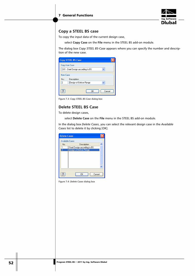
Create a new STEEL BS case To create a new design case,

select New Case on the File menu in the STEEL BS add-on module.

The following dialog box appears.

Figure 7.1: New STEEL BS-Case dialog box

In this dialog box, enter a No. (which is not yet assigned) and a Description for the new de-sign case. When you click [OK], table 1.1 General Data opens where you can enter the new design data.

Rename a STEEL BS case To change the description of a design case subsequently,

select Rename Case on the File menu in the STEEL BS add-on module.

The dialog box Rename STEEL BS-Case appears.

Figure 7.2: Rename STEEL BS-Case dialog box

7 General Functions


Copy a STEEL BS case To copy the input data of the current design case,

select Copy Case on the File menu in the STEEL BS add-on module.

The dialog box Copy STEEL BS-Case appears where you can specify the number and descrip-tion of the new case.

Figure 7.3: Copy STEEL BS-Case dialog box

Delete STEEL BS Case To delete design cases,

select Delete Case on the File menu in the STEEL BS add-on module.

In the dialog box Delete Cases, you can select the relevant design case in the Available Cases list to delete it by clicking [OK].

Figure 7.4: Delete Cases dialog box

7 General Functions


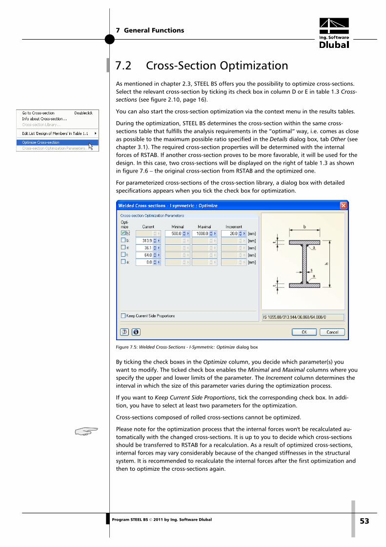
7.2 Cross-Section Optimization As mentioned in chapter 2.3, STEEL BS offers you the possibility to optimize cross-sections. Select the relevant cross-section by ticking its check box in column D or E in table 1.3 Cross-sections (see figure 2.10, page 16).

You can also start the cross-section optimization via the context menu in the results tables.

During the optimization, STEEL BS determines the cross-section within the same cross-sections table that fulfills the analysis requirements in the “optimal“ way, i.e. comes as close as possible to the maximum possible ratio specified in the Details dialog box, tab Other (see chapter 3.1). The required cross-section properties will be determined with the internal forces of RSTAB. If another cross-section proves to be more favorable, it will be used for the design. In this case, two cross-sections will be displayed on the right of table 1.3 as shown in figure 7.6 – the original cross-section from RSTAB and the optimized one.

For parameterized cross-sections of the cross-section library, a dialog box with detailed specifications appears when you tick the check box for optimization.

Figure 7.5: Welded Cross-Sections - I-Symmetric: Optimize dialog box

By ticking the check boxes in the Optimize column, you decide which parameter(s) you want to modify. The ticked check box enables the Minimal and Maximal columns where you specify the upper and lower limits of the parameter. The Increment column determines the interval in which the size of this parameter varies during the optimization process.

If you want to Keep Current Side Proportions, tick the corresponding check box. In addi-tion, you have to select at least two parameters for the optimization.

Cross-sections composed of rolled cross-sections cannot be optimized.

Please note for the optimization process that the internal forces won't be recalculated au-tomatically with the changed cross-sections. It is up to you to decide which cross-sections should be transferred to RSTAB for a recalculation. As a result of optimized cross-sections, internal forces may vary considerably because of the changed stiffnesses in the structural system. It is recommended to recalculate the internal forces after the first optimization and then to optimize the cross-sections again.

7 General Functions


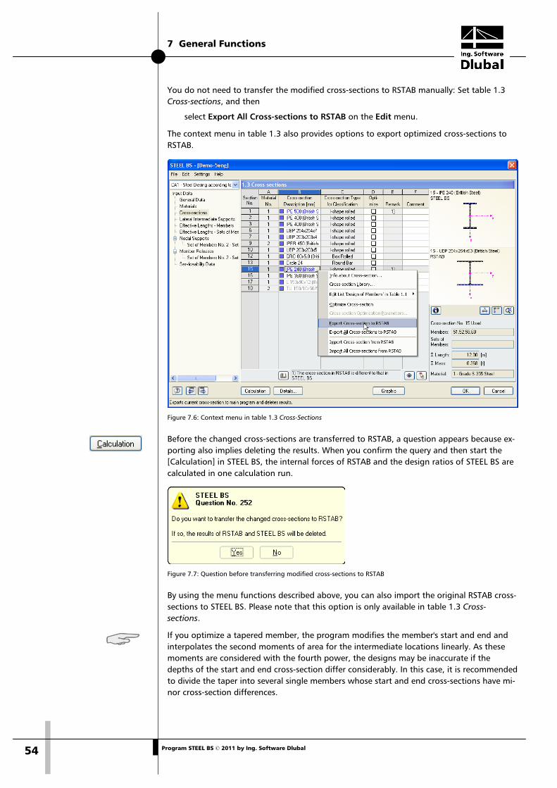
You do not need to transfer the modified cross-sections to RSTAB manually: Set table 1.3 Cross-sections, and then

select Export All Cross-sections to RSTAB on the Edit menu.

The context menu in table 1.3 also provides options to export optimized cross-sections to RSTAB.

Figure 7.6: Context menu in table 1.3 Cross-Sections

Before the changed cross-sections are transferred to RSTAB, a question appears because ex-porting also implies deleting the results. When you confirm the query and then start the [Calculation] in STEEL BS, the internal forces of RSTAB and the design ratios of STEEL BS are calculated in one calculation run.

Figure 7.7: Question before transferring modified cross-sections to RSTAB

By using the menu functions described above, you can also import the original RSTAB cross-sections to STEEL BS. Please note that this option is only available in table 1.3 Cross-sections.

If you optimize a tapered member, the program modifies the member's start and end and interpolates the second moments of area for the intermediate locations linearly. As these moments are considered with the fourth power, the designs may be inaccurate if the depths of the start and end cross-section differ considerably. In this case, it is recommended to divide the taper into several single members whose start and end cross-sections have mi-nor cross-section differences.

7 General Functions


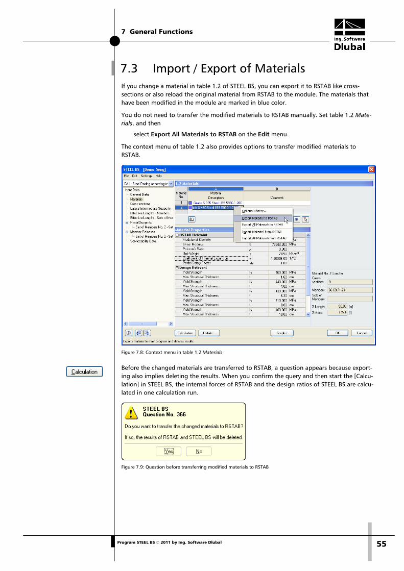
7.3 Import / Export of Materials If you change a material in table 1.2 of STEEL BS, you can export it to RSTAB like cross-sections or also reload the original material from RSTAB to the module. The materials that have been modified in the module are marked in blue color.

You do not need to transfer the modified materials to RSTAB manually. Set table 1.2 Mate-rials, and then

select Export All Materials to RSTAB on the Edit menu.

The context menu of table 1.2 also provides options to transfer modified materials to RSTAB.

Figure 7.8: Context menu in table 1.2 Materials

Before the changed materials are transferred to RSTAB, a question appears because export-ing also implies deleting the results. When you confirm the query and then start the [Calcu-lation] in STEEL BS, the internal forces of RSTAB and the design ratios of STEEL BS are calcu-lated in one calculation run.

Figure 7.9: Question before transferring modified materials to RSTAB

7 General Functions


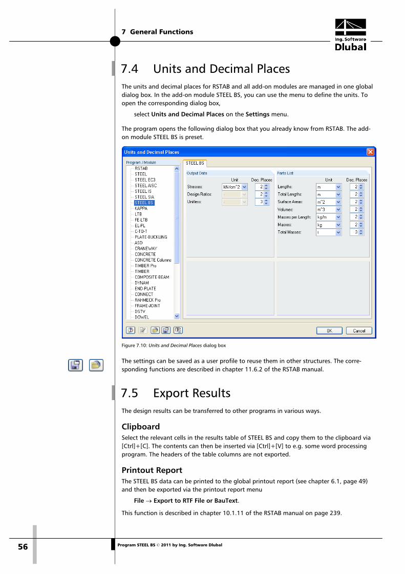
7.4 Units and Decimal Places The units and decimal places for RSTAB and all add-on modules are managed in one global dialog box. In the add-on module STEEL BS, you can use the menu to define the units. To open the corresponding dialog box,

select Units and Decimal Places on the Settings menu.

The program opens the following dialog box that you already know from RSTAB. The add-on module STEEL BS is preset.

Figure 7.10: Units and Decimal Places dialog box

The settings can be saved as a user profile to reuse them in other structures. The corre-sponding functions are described in chapter 11.6.2 of the RSTAB manual.

7.5 Export Results The design results can be transferred to other programs in various ways.

Clipboard Select the relevant cells in the results table of STEEL BS and copy them to the clipboard via [Ctrl]+[C]. The contents can then be inserted via [Ctrl]+[V] to e.g. some word processing program. The headers of the table columns are not exported.

Printout Report The STEEL BS data can be printed to the global printout report (see chapter 6.1, page 49) and then be exported via the printout report menu

File → Export to RTF File or BauText.

This function is described in chapter 10.1.11 of the RSTAB manual on page 239.

7 General Functions


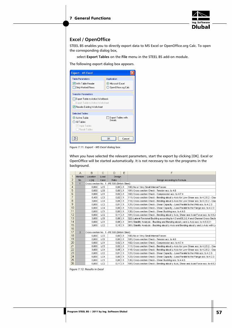
Excel / OpenOffice STEEL BS enables you to directly export data to MS Excel or OpenOffice.org Calc. To open the corresponding dialog box,

select Export Tables on the File menu in the STEEL BS add-on module.

The following export dialog box appears.

Figure 7.11: Export - MS Excel dialog box

When you have selected the relevant parameters, start the export by clicking [OK]. Excel or OpenOffice will be started automatically. It is not necessary to run the programs in the background.

Figure 7.12: Results in Excel

8 Example


8. Example

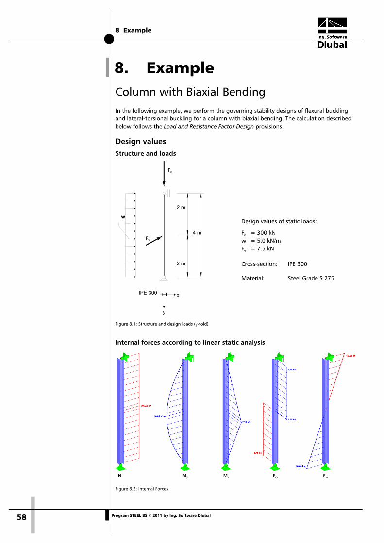
Column with Biaxial Bending In the following example, we perform the governing stability designs of flexural buckling and lateral-torsional buckling for a column with biaxial bending. The calculation described below follows the Load and Resistance Factor Design provisions.

Design values Structure and loads

Figure 8.1: Structure and design loads (γ-fold)

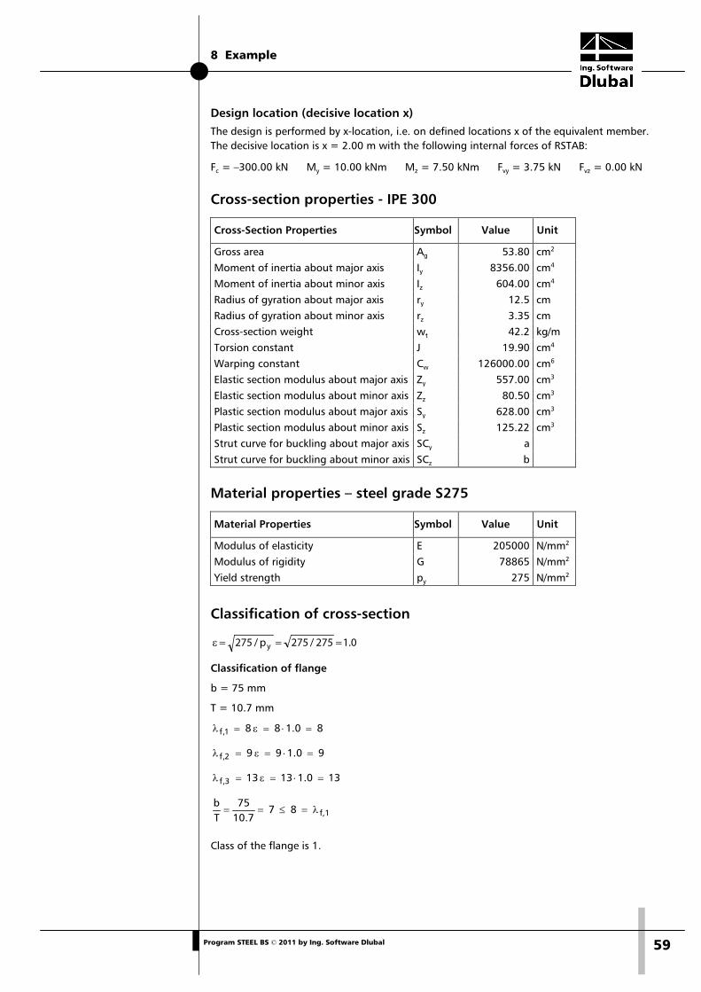
Internal forces according to linear static analysis

N My Mz Fvy Fvz

Figure 8.2: Internal Forces

w

2 m

2 m

Fv

Fc

z

y

IPE 300

4 m

Design values of static loads:

Fc = 300 kN w = 5.0 kN/m Fv = 7.5 kN Cross-section: IPE 300 Material: Steel Grade S 275

8 Example


Design location (decisive location x) The design is performed by x-location, i.e. on defined locations x of the equivalent member. The decisive location is x = 2.00 m with the following internal forces of RSTAB:

Fc = –300.00 kN My = 10.00 kNm Mz = 7.50 kNm Fvy = 3.75 kN Fvz = 0.00 kN

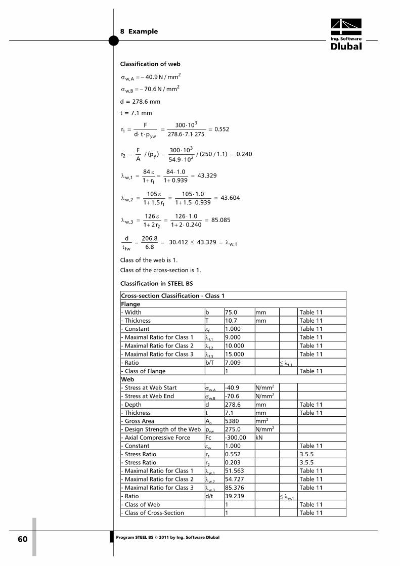
Cross-section properties - IPE 300

Cross-Section Properties Symbol Value Unit

Gross area Ag 53.80 cm2 Moment of inertia about major axis Iy 8356.00 cm4 Moment of inertia about minor axis Iz 604.00 cm4 Radius of gyration about major axis ry 12.5 cm Radius of gyration about minor axis rz 3.35 cm Cross-section weight wt 42.2 kg/m Torsion constant J 19.90 cm4 Warping constant Cw 126000.00 cm6 Elastic section modulus about major axis Zy 557.00 cm3 Elastic section modulus about minor axis Zz 80.50 cm3 Plastic section modulus about major axis Sy 628.00 cm3 Plastic section modulus about minor axis Sz 125.22 cm3

Strut curve for buckling about major axis SCy a Strut curve for buckling about minor axis SCz b

Material properties – steel grade S275

Material Properties Symbol Value Unit

Modulus of elasticity E 205000 N/mm2 Modulus of rigidity G 78865 N/mm2 Yield strength py 275 N/mm2

Classification of cross-section

1.0 275 / 275 p / 275 y ===ε

Classification of flange

b = 75 mm

T = 10.7 mm

8 1.08 8 1,f =⋅=ε=λ

9 1.0 9 9 2,f =⋅=ε=λ

13 1.0 13 13 3,f =⋅=ε=λ

f,1 8 7 7.10

75Tb

λ=≤==

Class of the flange is 1.

8 Example


Classification of web

2Aw, mm / N 40.9 −=σ

2Bw, mm / N .607 −=σ

d = 278.6 mm

t = 7.1 mm

0.552 275 7.1 278.6

10 300

p t dF

r3

yw1 =

⋅⋅⋅

=⋅⋅

=

0.240 1.1) / (250 / 10 54.9

10 300 )(p /

AF

r2

3

y2 =⋅

⋅==

43.329 0.939 1

1.0 84

r1 84

1

1,w =+

⋅=

+ε

=λ

43.604 0.939 1.5 11.0 105

r 5.11

105

12,w =

⋅+⋅

=+

ε=λ

85.085 0.240 2 11.0 126

r 21 126

2

3,w =⋅+⋅

=+

ε=λ

w,1fw

43.329 412.30 8.6

8.206

td

λ=≤==

Class of the web is 1.

Class of the cross-section is 1.

Classification in STEEL BS

Cross-section Classification - Class 1 Flange - Width b 75.0 mm Table 11 - Thickness T 10.7 mm Table 11 - Constant εf 1.000 Table 11 - Maximal Ratio for Class 1 λf,1 9.000 Table 11 - Maximal Ratio for Class 2 λf,2 10.000 Table 11 - Maximal Ratio for Class 3 λf,3 15.000 Table 11 - Ratio b/T 7.009 ≤ λf,1 - Class of Flange 1 Table 11 Web - Stress at Web Start σw,A -40.9 N/mm2 - Stress at Web End σw,B -70.6 N/mm2 - Depth d 278.6 mm Table 11 - Thickness t 7.1 mm Table 11 - Gross Area Ag 5380 mm2 - Design Strength of the Web pyw 275.0 N/mm2 - Axial Compressive Force Fc -300.00 kN - Constant εw 1.000 Table 11 - Stress Ratio r1 0.552 3.5.5 - Stress Ratio r2 0.203 3.5.5 - Maximal Ratio for Class 1 λw,1 51.563 Table 11 - Maximal Ratio for Class 2 λw,2 54.727 Table 11 - Maximal Ratio for Class 3 λw,3 85.376 Table 11 - Ratio d/t 39.239 ≤ λw,1 - Class of Web 1 Table 11 - Class of Cross-Section 1 Table 11

8 Example


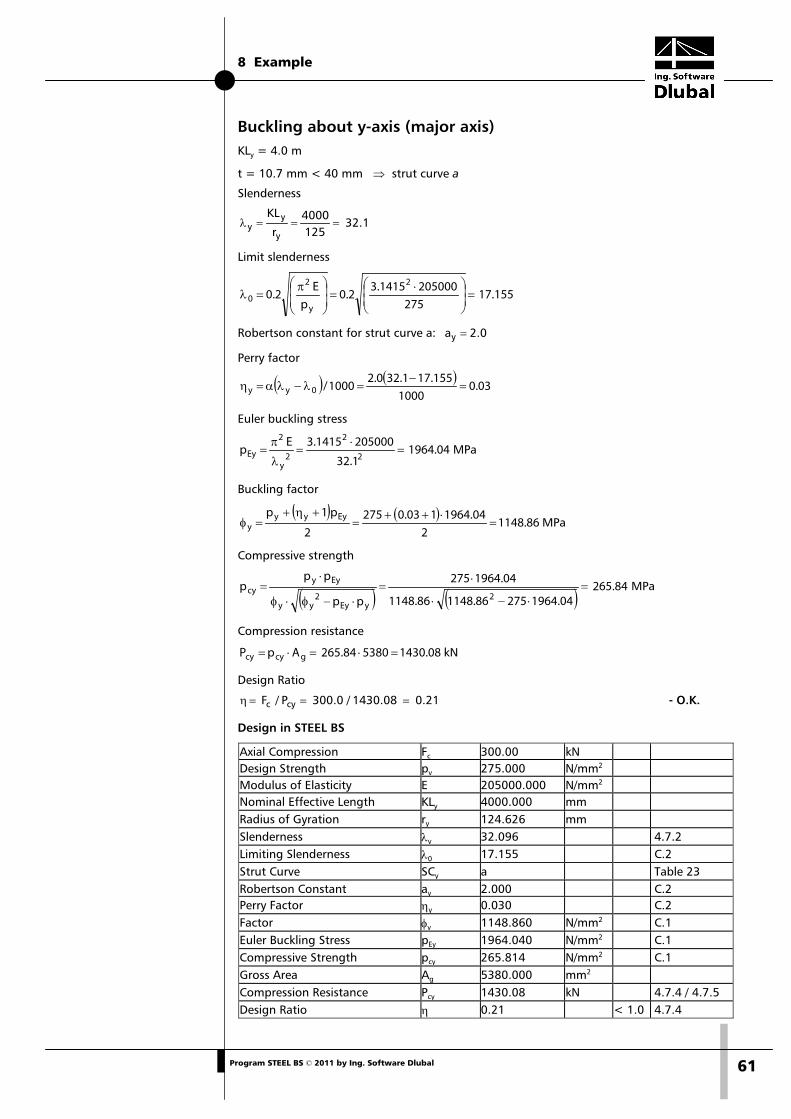
Buckling about y-axis (major axis) KLy = 4.0 m

t = 10.7 mm < 40 mm ⇒ strut curve a

Slenderness

32.1 1254000

r

KL

y

yy ===λ

Limit slenderness

17.155 275

205000 1415.32.0

pE

2.0 2

y

2

0 =

⋅=

π=λ

Robertson constant for strut curve a: 0.2 ay =

Perry factor

( ) ( )03.0

1000155.171.320.2

1000/ 0yy =−

=λ−λα=η

Euler buckling stress

1964.04 1.32

205000 1415.3E p

2

2

2y

2

Ey =⋅

=λ

π= MPa

Buckling factor

( ) ( )86.1148

21964.04 103.0275

2

p 1p

Eyyyy =

⋅++=

+η+=φ MPa

Compressive strength

( ) ( )265.84

1964.04 27586.1148 86.1148

1964.04 275

p p

p p p

2yEy

2yy

Eyycy =

⋅−⋅

⋅=

⋅−φ⋅φ

⋅= MPa

Compression resistance

1430.085380 265.84 A pP gcycy =⋅=⋅= kN

Design Ratio

0.21 1430.08 / 300.0 P / F cyc ===η - O.K.

Design in STEEL BS

Axial Compression Fc 300.00 kN Design Strength py 275.000 N/mm2 Modulus of Elasticity E 205000.000 N/mm2 Nominal Effective Length KLy 4000.000 mm Radius of Gyration ry 124.626 mm Slenderness λy 32.096 4.7.2 Limiting Slenderness λ0 17.155 C.2 Strut Curve SCy a Table 23 Robertson Constant ay 2.000 C.2 Perry Factor ηy 0.030 C.2 Factor φy 1148.860 N/mm2 C.1 Euler Buckling Stress pEy 1964.040 N/mm2 C.1 Compressive Strength pcy 265.814 N/mm2 C.1 Gross Area Ag 5380.000 mm2 Compression Resistance Pcy 1430.08 kN 4.7.4 / 4.7.5 Design Ratio η 0.21 < 1.0 4.7.4

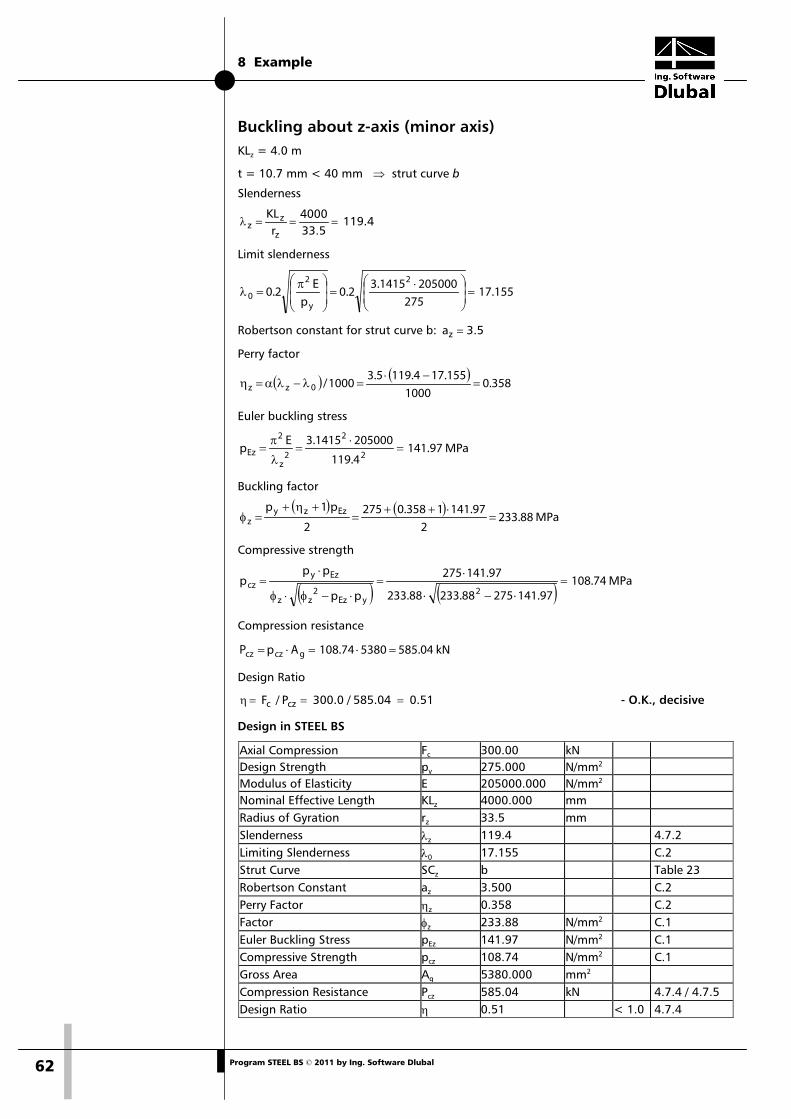
8 Example


Buckling about z-axis (minor axis) KLz = 4.0 m

t = 10.7 mm < 40 mm ⇒ strut curve b

Slenderness

119.4 33.54000

r

KL

z

zz ===λ

Limit slenderness

17.155 275

205000 1415.32.0

pE

2.0 2

y

2

0 =

⋅=

π=λ

Robertson constant for strut curve b: 5.3 az =

Perry factor

( ) ( )358.0

1000155.174.119 5.3

1000/ 0zz =−⋅

=λ−λα=η

Euler buckling stress

141.97 4.119

205000 1415.3E p

2

2

2z

2

Ez =⋅

=λ

π= MPa

Buckling factor

( ) ( )88.233

297.141 1358.0275

2

p 1p

Ezzyz =

⋅++=

+η+=φ MPa

Compressive strength

( ) ( )108.74

141.97 27588.233 33.882

141.97 275

p p

p p p

2yEz

2zz

Ezycz =

⋅−⋅

⋅=

⋅−φ⋅φ

⋅= MPa

Compression resistance

585.045380 108.74 A pP gczcz =⋅=⋅= kN

Design Ratio

0.51 585.04 / 300.0 P / F czc ===η - O.K., decisive

Design in STEEL BS

Axial Compression Fc 300.00 kN Design Strength py 275.000 N/mm2 Modulus of Elasticity E 205000.000 N/mm2 Nominal Effective Length KLz 4000.000 mm Radius of Gyration rz 33.5 mm Slenderness λz 119.4 4.7.2 Limiting Slenderness λ0 17.155 C.2 Strut Curve SCz b Table 23 Robertson Constant az 3.500 C.2 Perry Factor ηz 0.358 C.2 Factor φz 233.88 N/mm2 C.1 Euler Buckling Stress pEz 141.97 N/mm2 C.1 Compressive Strength pcz 108.74 N/mm2 C.1 Gross Area Ag 5380.000 mm2 Compression Resistance Pcz 585.04 kN 4.7.4 / 4.7.5 Design Ratio η 0.51 < 1.0 4.7.4

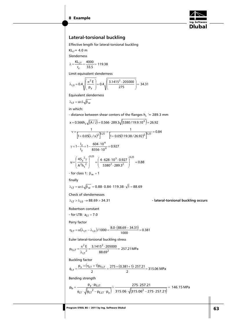
8 Example


Lateral-torsional buckling Effective length for lateral-torsional buckling

KLLT= 4.0 m

Slenderness

119.38 33.54000

r

KL

z

LT ===λ

Limit equivalent slenderness

34.31 275

205000 1415.34.0

pE

4.0 2

y

2

0L =

⋅=

π=λ

Equivalent slenderness

wLT u βνλ=λ

in which:

- distance between shear centers of the flanges hs = 289.3 mm

( ) ( ) 92.2610.9.19/5380289.3 566.0J/Ah566.0x 4s =⋅==

( )[ ] ( )[ ] 84.0

92.26/38.11905.01

1

x/05.01

125.0225.02

=+

=λ+

=ν

927.0108356

106041

I

I1

4

4

y

z =⋅

⋅−=−=γ

88.0289.3 5380

0.927 10628 4

hA

S4u

25.0

22

325.0

2s

2

2y =

⋅

⋅⋅⋅=

γ=

- for class 1: 1w =β

finally

69.88138.11984.088.0u wLT =⋅⋅⋅=βνλ=λ

Check of slendernesses

31.3469.88 0LLT >→λ>λ - lateral-torsional buckling occurs

Robertson constant

- for LTB: 0.7 aLT =

Perry factor

( ) ( )381.0

100031.3469.88 0.8

1000/ 0LLTLT =−⋅

=λ−λα=η

Euler lateral-torsional buckling stress

257.21 69.88

205000 1415.3E p

2

2

2LT

2

LT,E =⋅

=λ

π= MPa

Buckling factor

( ) ( )06.315

257.212 1381.0275

2

p 1p

LT,ELTyLT =

⋅++=

+η+=φ MPa

Bending strength

( ) ( ) 146.15 257.21 27506.315 15.063

257.21 275´

p p

p p p

2yLT,E

2LTLT

LT,Eyb =

⋅−⋅

⋅=

⋅−φ⋅φ

⋅= MPa

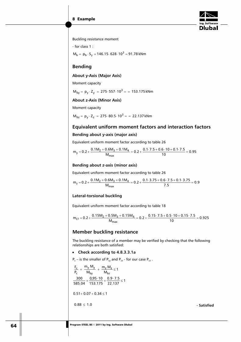
8 Example


Buckling resistance moment

- for class 1 :

78.911062815.146S p M 3ybb =⋅⋅=⋅= kNm

Bending

About y-Axis (Major Axis)

Moment capacity

kNm 153.175 10557752 Zp M 3yyby´ ==⋅⋅=⋅=

About z-Axis (Minor Axis)

Moment capacity

kNm 22.137 105.08752 Zp M 3zybz´ ==⋅⋅=⋅=

Equivalent uniform moment factors and interaction factors Bending about y-axis (major axis)

Equivalent uniform moment factor according to table 26

95.010

5.71.0106.05.71.02.0

M0.1M0.6M0.1M

.20 mmax

432y =

⋅+⋅+⋅+=

+++=

Bending about z-axis (minor axis)


9.05.7

75.31.05.76.075.31.02.0

M0.1M0.6M0.1M

.20 mmax

432z =

⋅+⋅+⋅+=

+++=

Lateral-torsional buckling


925.010

5.715.0105.05.715.02.0

M0.15M0.5M0.15M

.20 mmax

432LT =

⋅+⋅+⋅+=

+++=

Member buckling resistance

The buckling resistance of a member may be verified by checking that the following relationships are both satisfied:

• Check according to 4.8.3.3.1a

Pc – is the smaller of Pcy and Pcz - for our case Pcz .

1.0 0.88

134.007.051.0

1137.22

5.79.0175.1531095,0

04.585300

1 M

M m

M

M m

PF

bz

zz

by

yy

c

c

≤

≤++

≤⋅

+⋅

+

≤++

- Satisfied

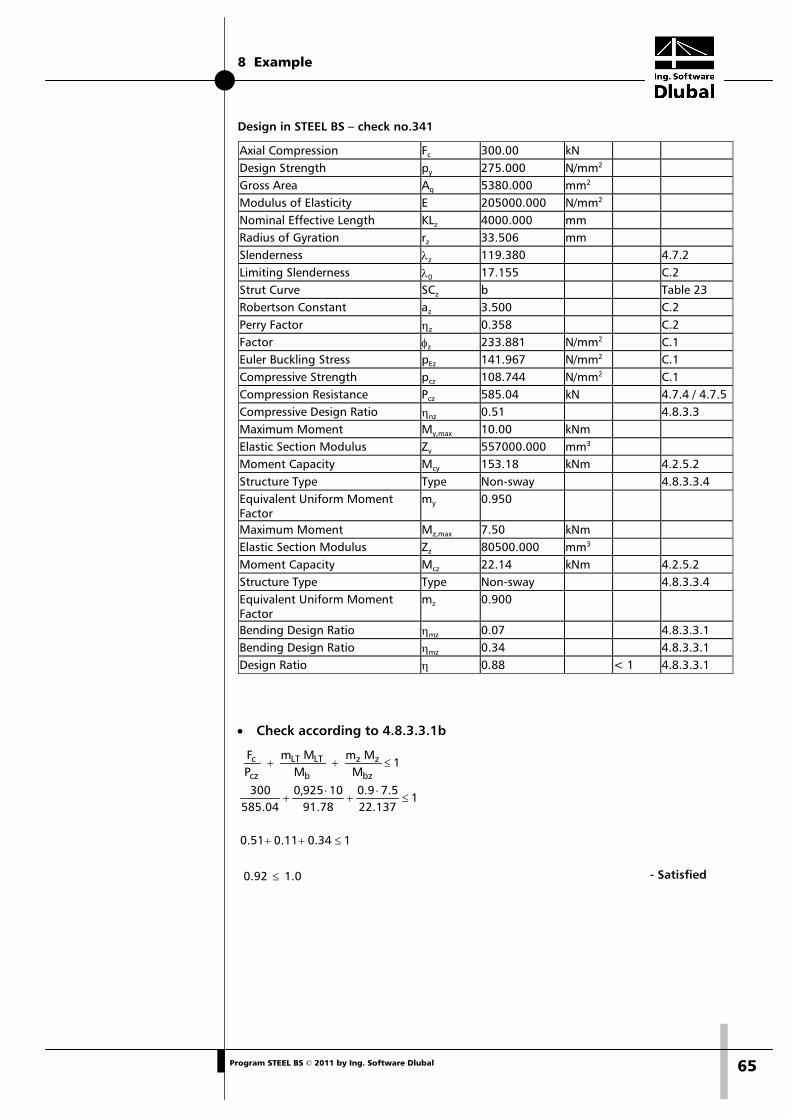
8 Example


Design in STEEL BS – check no.341

Axial Compression Fc 300.00 kN Design Strength py 275.000 N/mm2 Gross Area Ag 5380.000 mm2 Modulus of Elasticity E 205000.000 N/mm2 Nominal Effective Length KLz 4000.000 mm Radius of Gyration rz 33.506 mm Slenderness λz 119.380 4.7.2 Limiting Slenderness λ0 17.155 C.2 Strut Curve SCz b Table 23 Robertson Constant az 3.500 C.2 Perry Factor ηz 0.358 C.2 Factor φz 233.881 N/mm2 C.1 Euler Buckling Stress pEz 141.967 N/mm2 C.1 Compressive Strength pcz 108.744 N/mm2 C.1 Compression Resistance Pcz 585.04 kN 4.7.4 / 4.7.5 Compressive Design Ratio ηnz 0.51 4.8.3.3 Maximum Moment My,max 10.00 kNm Elastic Section Modulus Zy 557000.000 mm3 Moment Capacity Mcy 153.18 kNm 4.2.5.2 Structure Type Type Non-sway 4.8.3.3.4 Equivalent Uniform Moment Factor

my 0.950

Maximum Moment Mz,max 7.50 kNm Elastic Section Modulus Zz 80500.000 mm3 Moment Capacity Mcz 22.14 kNm 4.2.5.2 Structure Type Type Non-sway 4.8.3.3.4 Equivalent Uniform Moment Factor

mz 0.900

Bending Design Ratio ηmz 0.07 4.8.3.3.1 Bending Design Ratio ηmz 0.34 4.8.3.3.1 Design Ratio η 0.88 < 1 4.8.3.3.1

• Check according to 4.8.3.3.1b

1.0 0.92

134.011.051.0

1137.22

5.79.078.91

10925,004.585

300

1 M

M m

MM m

PF

bz

zz

b

LTLT

cz

c

≤

≤++

≤⋅

+⋅

+

≤++

- Satisfied

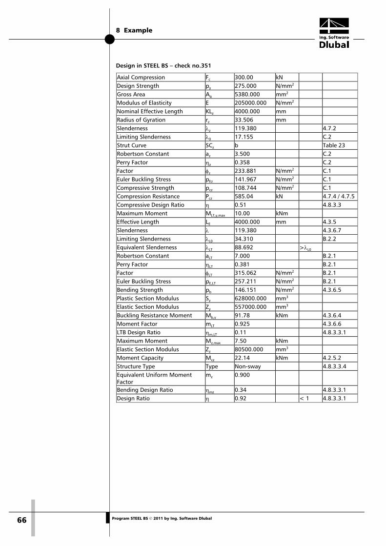
8 Example


Design in STEEL BS – check no.351

Axial Compression Fc 300.00 kN Design Strength py 275.000 N/mm2 Gross Area Ag 5380.000 mm2 Modulus of Elasticity E 205000.000 N/mm2 Nominal Effective Length KLz 4000.000 mm Radius of Gyration rz 33.506 mm Slenderness λz 119.380 4.7.2 Limiting Slenderness λ0 17.155 C.2 Strut Curve SCz b Table 23 Robertson Constant az 3.500 C.2 Perry Factor ηz 0.358 C.2 Factor φz 233.881 N/mm2 C.1 Euler Buckling Stress pEz 141.967 N/mm2 C.1 Compressive Strength pcz 108.744 N/mm2 C.1 Compression Resistance Pcz 585.04 kN 4.7.4 / 4.7.5 Compressive Design Ratio η 0.51 4.8.3.3 Maximum Moment MLT,y,max 10.00 kNm Effective Length LE 4000.000 mm 4.3.5 Slenderness λ 119.380 4.3.6.7 Limiting Slenderness λL0 34.310 B.2.2 Equivalent Slenderness λLT 88.692 >λL0 Robertson Constant aLT 7.000 B.2.1 Perry Factor ηLT 0.381 B.2.1 Factor φLT 315.062 N/mm2 B.2.1 Euler Buckling Stress pE,LT 257.211 N/mm2 B.2.1 Bending Strength pb 146.151 N/mm2 4.3.6.5 Plastic Section Modulus Sy 628000.000 mm3 Elastic Section Modulus Zy 557000.000 mm3 Buckling Resistance Moment Mb,y 91.78 kNm 4.3.6.4 Moment Factor mLT 0.925 4.3.6.6 LTB Design Ratio ηm,LT 0.11 4.8.3.3.1 Maximum Moment Mz,max 7.50 kNm Elastic Section Modulus Zz 80500.000 mm3 Moment Capacity Mcz 22.14 kNm 4.2.5.2 Structure Type Type Non-sway 4.8.3.3.4 Equivalent Uniform Moment Factor

mz 0.900

Bending Design Ratio ηmz 0.34 4.8.3.3.1 Design Ratio η 0.92 < 1 4.8.3.3.1

A Literature


A Literature

[1] Structural use of steelwork in buildings – Part1: Code of practice for design – Rolled and Welded sections, BS 5950-1:2000, BS 05-2001

[2] Eurocode 3: Design of steel structures – Part 1-1: General rules and rules for buildings, 2005

[3] Rules for Member Stability in EN 1993-1-1, ECCS Technical Committee 8 – Stability

[4] Eurocode 3: Design of steel structures – Part 1-4: Supplementary rules for Stainless steels, 2006

[5] Die neuen Stabilitätsnachweise im Stahlbau nach Eurocode 3, NAUMES J., STROHMANN I., UNGERMANN D., SEDLACEK G., Stahlbau 77 (2008) Heft 10, Ernst & Sohn

B Index


B Index B

Background graphics ................................... 42

Buckling about axis ...................................... 23

Buckling length coefficient .................... 22, 23

Buckling possible ......................................... 23

Buttons ........................................................ 41

C

Calculation ................................................... 29

Camber ........................................................ 28

Cantilever beam ..................................... 20, 28

Charakteristic ............................................... 10

Classification ................................................ 19

Close STEEL BS ............................................... 8

Color bars .................................................... 41

Color spectrum ............................................ 47

Colored ratios .............................................. 47

Column buckling ................................... 20, 21

Control panel ............................................... 47

Coordinate system ....................................... 16

Cross-section description ............................. 16

Cross-section library............................... 16, 17

Cross-section optimization .......................... 53

Cross-section parts (c/t) ............................... 18

Cross-sections .............................................. 16

D

Decimal places ....................................... 14, 56

Deflection .................................................... 10

Deformation ................................................ 30

Design ........................................................... 9

Design by cross-section ............................... 34

Design by load case ..................................... 33

Design case ...................................... 43, 51, 52

Design combination ..................................... 10

Design ratio ................................................. 34

Design situation ........................................... 34

Details .......................................................... 29

Display hidden result diagram ..................... 47

Display navigator ................................... 43, 47

E

Effective length ...................................... 21, 22

Effective Slenderness .................................... 39

Elastic critical moment ................................. 30

Equivalent uniform moment factor .............. 24

Evaluation of results ..................................... 41

Excel ............................................................. 57

Export cross-section ..................................... 54

Export material ............................................. 55

Export materials ........................................... 55

Export results ............................................... 56

F

Filter members ............................................. 48

Filter results .................................................. 47

Forked support ............................................. 20

Frequent ....................................................... 10

G

General data................................................... 8

Governing internal forces ............................. 37

Graph of results ........................................... 46

Graphic ........................................................ 42

I

Installation ..................................................... 5

Internal forces .............................................. 53

L

Lateral intermediate supports ...................... 20

Lateral-torsional buckling ................. 11, 20, 24

Length .................................................... 21, 39

Limit load ..................................................... 30

Limit values .................................................. 10

List of members ............................................ 28

Load application ........................................... 30

Load case ................................................. 9, 10

Load combination ........................................ 10

Location x ......................................... 34, 36, 37

M

Material description ..................................... 14

Material library ............................................. 15

Material properties ....................................... 14

Materials ...................................................... 14

Maximum design ratio ................................. 19

Member diagrams ........................................ 45

B Index


Member release ........................................... 27

Members ....................................................... 9

N

National annex ............................................ 11

Naumes ....................................................... 11

Navigator ....................................................... 8

Nodal support.............................................. 25

Non-sway ..................................................... 30

O

OpenOffice .................................................. 57

Optimization .................................... 19, 30, 53

P

Panel .................................................. 7, 44, 47

Parameterized cross-section ........................ 53

Part .............................................................. 39

Partial view .................................................. 47

Parts list ....................................................... 39

Print ............................................................. 49

Print STEEL BS graphics ................................ 49

Printout report ................................. 49, 50, 56

Q

Quasi-permanent ......................................... 10

R

Reference length .......................................... 28

Relatively ..................................................... 20

Release ......................................................... 27

Remark ........................................................ 19

Rendering ratios .......................................... 47

Result diagram ....................................... 46, 49

Result values ................................................ 43

Results representation ................................. 43

Results tables ............................................... 33

RSBUCK ........................................................ 22

RSTAB graphic ............................................. 49

RSTAB work window.................................... 42

S

Safety factors ............................................... 11

Scaling .......................................................... 45

Serviceability design ..................................... 28

Serviceability limit state .......................... 10, 30

Set of members ......... 9, 24, 25, 27, 35, 38, 40

Shifted member ends ................................... 30

Slenderness .................................................. 38

Stability analysis ........................................... 11

Stainless steel ............................................... 13

Start calculation ........................................... 31

Start STEEL BS ................................................ 6

STEEL BS design cases .................................. 51

Stress point ............................................ 17, 18

Structure type .............................................. 30

Sum .............................................................. 40

Support ........................................................ 25

Surface area ................................................. 40

Sway ............................................................. 30

Switch tables .................................................. 8

T

Tables ............................................................. 8

Taper ............................................................ 54

Tapered member .................................... 17, 34

U

Ultimate limit state......................................... 8

Undeformed system ..................................... 30

Unit weight .................................................. 40

Units ....................................................... 14, 56

User profile ................................................... 56

V

View mode ............................................. 41, 42

Visualization ................................................. 42

Volume ......................................................... 40

W

Weight ......................................................... 40

Add-on Module STEEL BS - Dlubal · PDF fileAdd-on Module STEEL BS ... BS 5950-1 and BS EN...

Documents

Transcript of Add-on Module STEEL BS - Dlubal · PDF fileAdd-on Module STEEL BS ... BS 5950-1 and BS EN...